Embed Size (px)
Citation preview
BB..CC.. IIRRRRIIGGAATTIIOONN MMAANNAAGGEEMMEENNTT GGUUIIDDEE
Chapter 6
Editor
Ted W. van der Gulik, P.Eng.
Authors
Stephanie Tam, B.A.Sc. T. Janine Nyvall, P.Eng. Lance Brown, Eng Tech
Prepared by
B.C. Ministry of Agriculture, Food and Fisheries Resource Management Branch
Published by
Irrigation Industry Association of British Columbia
2005 ISSUE
LIMITATION OF LIABILITY AND USER’S RESPONSIBILITY
The primary purpose of this B.C. Irrigation Management Guide is to provide irrigation professionals and consultants with a methodology to assess the irrigation system performance and manage the system effectively. While every effort has been made to ensure the accuracy and completeness of these materials, additional materials may be required to complete more advanced assessments. Advice of appropriate professionals and experts may assist in completing assessments that are not covered in this Guide. All information in this publication and related materials are provided entirely “as is” and no representations, warranties or conditions, either expressed or implied, are made in connection with your use of, or reliance upon, this information. This information is provided to you as the user entirely at your risk. The British Columbia Ministry of Agriculture, Food and Fisheries and the Irrigation Industry Association of British Columbia, their Directors, agents, employees, or contractors will not be liable for any claims, damages or losses of any kind whatsoever arising out of the use of, reliance upon, this information.
Chapter 6 Irrigation System Assessment 99
6 IRRIGATION SYSTEM ASSESSMENT It is essential that an irrigation system be designed to match the soil, crop and local climate conditions present if an irrigator is to achieve good irrigation management. This chapter provides information on how to select an irrigation system, assess irrigation system equipment and layout, and perform a system performance check. In many instances, improvements may be limited by the design of the irrigation system, making it difficult to improve system performance without redesigning the entire system. In such cases, it is recommended that a Certified Irrigation Designer (CID) be consulted. An irrigation system assessment should start by evaluating whether the current type of irrigation system is best suited for the crop, soil and field conditions present. If the system is appropriate, further assessment can be done to check the irrigation system uniformity. A good irrigator will operate the system long enough to ensure that the entire crop has received enough water. Irrigation systems that have poor uniformity will need to be run longer to ensure that the area with the lowest application rate receives enough water. An irrigation system that applies water uniformly will have lower watering times, and can then be managed to achieve good water use efficiency. Separate sections are provided for conducting irrigation system assessments for:
sprinkler travelling gun, and trickle/drip systems.
An irrigation assessment that ensures proper system performance and maximum uniformity should be done before an efficient irrigation schedule (Chapter 7) can be determined.
100
6.1 Selection of an Irrigation System
Options Proper selection of an irrigation system includes taking into consideration system type, design, operation and maintenance. The type of irrigation system most suitable for a particular site depends on crop characteristics, climate, soil and site conditions. A brief description of each system follows.
Irrigation Systems at a Glance
Trickle/Drip Systems Trickle/drip systems are the most efficient method of irrigation if managed properly, but they are not suitable for all cropping systems. Trickle/drip systems are most applicable to horticultural crops, such as tree fruits, berries, grapes, vegetable and other plants grown in rows. Trickle systems can be designed to match almost any soil condition providing that plant root volume and lateral movement of water in the soil is considered. Water of poor quality will require filtration systems to ensure that the system is able to operate properly. In this Guide, trickle refers to frequent, low-pressure application of water to crops, including
B.C. Irrigation Management Guide
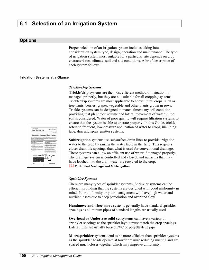
tape, drip and spray emitter systems. Subirrigation systems use subsurface drain lines to provide irrigation water to the crop by raising the water table in the field. This requires closer drain tile spacings than what is used for conventional drainage. These systems can allow an efficient use of water if managed properly. The drainage system is controlled and closed, and nutrients that may have leached into the drain water are recycled to the crop.
Controlled Drainage and Subirrigation
Sprinkler Systems There are many types of sprinkler systems. Sprinkler systems can be efficient providing that the systems are designed with good uniformity in mind. Poor uniformity or poor management will have high water and nutrient losses due to deep percolation and overland flow. Handmove and wheelmove systems generally have standard sprinkler spacings as aluminum pipes of standard lengths are usually used. Overhead or Undertree solid set systems can have a variety of sprinkler spacings as the sprinkler layout must match the crop spacings. Lateral lines are usually buried PVC or polyethylene pipe. Microsprinkler systems tend to be more efficient than sprinkler systems as the sprinkler heads operate at lower pressure reducing misting and are spaced much closer together which may improve uniformity.
Chapter 6 Irrigation System Assessment 101
Large Volume Sprinkler or Gun Systems Guns systems operate at much higher flows and pressures than regular sprinkler systems. Increased wind drift results in higher evaporation losses and lower operating efficiencies than the smaller sprinkler systems. Stationary guns generally have a very high application rate. The set times for these systems should be very short to avoid deep percolation or runoff. The short set time makes these systems very difficult to manage properly. Travelling guns overcome the problem of the short set time for stationary guns by moving the gun over a large area during one set. They are still susceptible to wind drift and evaporation losses because of the high operating pressures required by the gun.
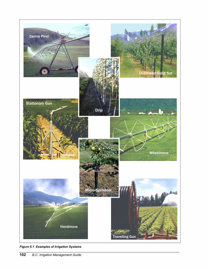
Other Systems Centre pivot systems can have higher efficiencies than sprinkler systems if low volume spray heads are used. The system travels around the field which makes it easier to match the water application to the crop and soil conditions. These systems are also automated which reduces the labour component and adds flexibility in management. Flood irrigation systems in British Columbia are usually not designed in a fashion that includes recycling of the tail water that is leaving the end of the field. Since fields are also not laser levelled, most flood systems in British Columbia are not very efficient. Figure 6.1 shows some examples of irrigation systems.
Factors Affecting Selection of Irrigation Systems The following factors should be considered when selecting an irrigation system:
field size and shape topography irrigation efficiency cost labour management maintenance
crop type pressure requirement water quality other uses:
frost protection crop cooling fertigation
Field Size and Topography The field size and configuration often dictates what type of system is suitable for that location. Centre pivot systems require large symmetrical parcels of land to operate effectively. Wheel lines operate best on rectangular-shaped properties that are at least 20 acres. Travelling guns are more flexible and can adjust to different field sizes and shapes.
102
Figur
S
Centre PivotB.C. Irrigation Management Guide
e 6.1 Examples of Irrigation Systems
tationary Gun
Handmove
Wheelmove
Drip
Micro-SprinklerTravelling Gun
Overhead Solid Set
Travelling Gun
Chapter 6 Irrigation System Assessment 103
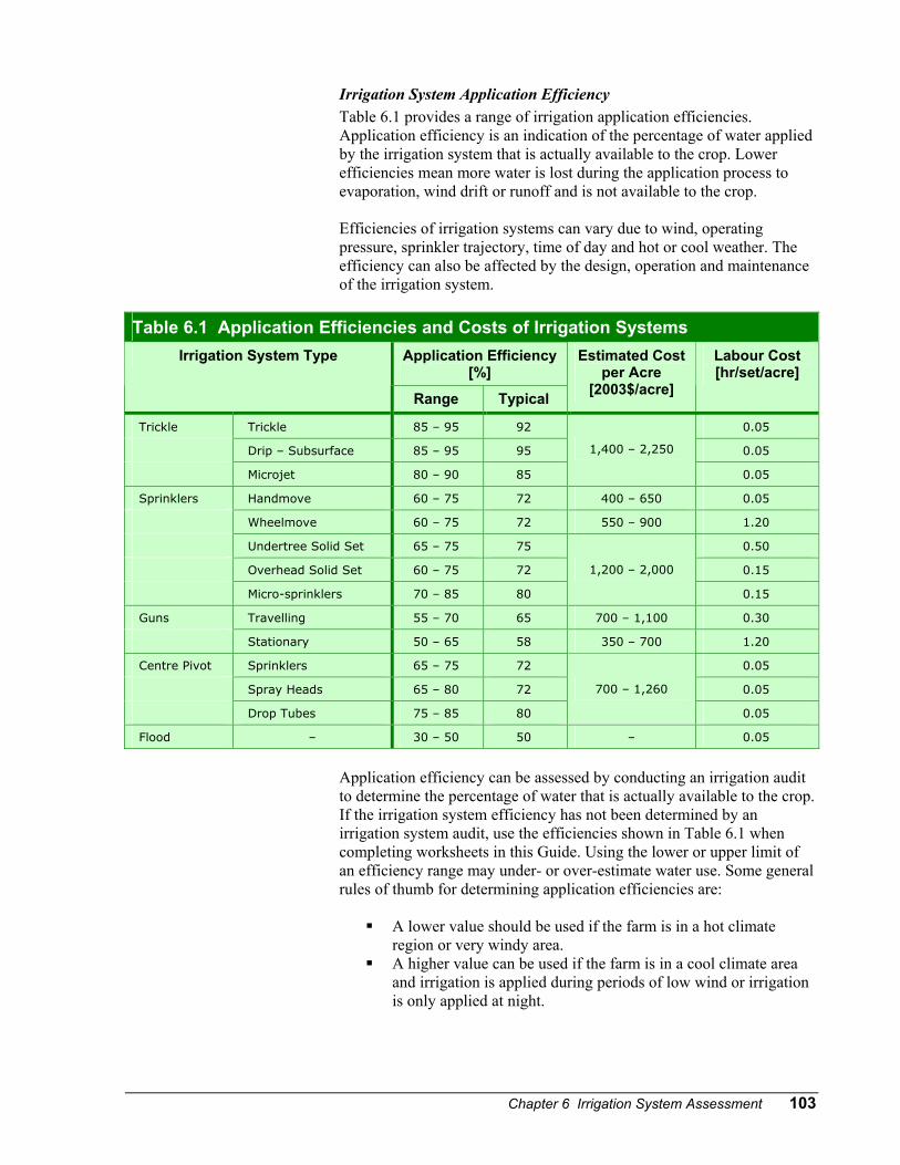
Irrigation System Application Efficiency Table 6.1 provides a range of irrigation application efficiencies. Application efficiency is an indication of the percentage of water applied by the irrigation system that is actually available to the crop. Lower efficiencies mean more water is lost during the application process to evaporation, wind drift or runoff and is not available to the crop. Efficiencies of irrigation systems can vary due to wind, operating pressure, sprinkler trajectory, time of day and hot or cool weather. The efficiency can also be affected by the design, operation and maintenance of the irrigation system.
Table 6.1 Application Efficiencies and Costs of Irrigation Systems Application Efficiency
[%] Irrigation System Type
Range Typical
Estimated Cost per Acre
[2003$/acre]
Labour Cost [hr/set/acre]
Trickle Trickle 85 – 95 92 0.05
Drip – Subsurface 85 – 95 95 0.05
Microjet 80 – 90 85
1,400 – 2,250
0.05
Sprinklers Handmove 60 – 75 72 400 – 650 0.05
Wheelmove 60 – 75 72 550 – 900 1.20
Undertree Solid Set 65 – 75 75 0.50
Overhead Solid Set 60 – 75 72 0.15
Micro-sprinklers 70 – 85 80
1,200 – 2,000
0.15
Guns Travelling 55 – 70 65 700 – 1,100 0.30
Stationary 50 – 65 58 350 – 700 1.20
Centre Pivot Sprinklers 65 – 75 72 0.05
Spray Heads 65 – 80 72 0.05
Drop Tubes 75 – 85 80
700 – 1,260
0.05
Flood – 30 – 50 50 – 0.05
Application efficiency can be assessed by conducting an irrigation audit to determine the percentage of water that is actually available to the crop. If the irrigation system efficiency has not been determined by an irrigation system audit, use the efficiencies shown in Table 6.1 when completing worksheets in this Guide. Using the lower or upper limit of an efficiency range may under- or over-estimate water use. Some general rules of thumb for determining application efficiencies are:
A lower value should be used if the farm is in a hot climate region or very windy area.
A higher value can be used if the farm is in a cool climate area and irrigation is applied during periods of low wind or irrigation is only applied at night.
104
Labour Automated systems such as trickle/drip, centre pivots and solid set sprinklers have low labour requirements compared to other systems. These systems do not have to be manually moved and irrigation scheduling changes can be done by adjusting the system control. Irrigation systems, such as wheelmoves, handmoves and guns require daily labour to move the system from one set to the next. The labour cost may also be increased if travel distance to the field is significant.
B.C. Irrigation Management Guide
Cost The capital cost of an irrigation system is often a major consideration when deciding on what type of system to purchase. However carefully considering annual maintenance, operating costs, labour, improved system management and water savings may make the more expensive systems more attractive in the long run.
Irrigation Equipment Costs 2003
Management and Maintenance System management and maintenance will vary with different system types, field topography, operating pressures, type of material (PVC, steel etc) and installation. All systems require regular maintenance, but automated systems are easier to manage.
Crop Type Crop type will often dictate what type of system will work best in a given situation. For example, a solid set system in a corn field is impractical for harvesting or cultivation. Also, a system that is low to the ground will not be able to spread water very far when the crop is taller than the irrigation nozzles. Trickle systems are best suited for horticultural and other row crops where water can be applied to a localized root zone.
Pressure Requirement Irrigation guns have a high pressure requirement to obtain proper stream dispersal while centre pivot and trickle systems can operate with very low pressure. The pressure requirement is also determined by elevation and pipe friction losses due to system flow rate. If the proper pressure requirement for a system cannot be delivered, a different system should be considered or adjustments to the design changed.
Water Quality Water of poor quality can sometimes cause staining on crops. This is undesirable for crops that are sold for fresh market or graded on appearance. Irrigation systems that do not spread water on the fruit, such as a trickle system, would be desirable in these cases. Water quality also affects the type of screening or filtration equipment that may be required. Water with high sediment content will wear nozzles, pipes, pump impellors and impellor shafts more quickly, increasing maintenance costs dramatically.
Other Uses If the system is used for purposes other than irrigation, e.g., crop cooling, frost protection or chemigation, these purposes must be considered when deciding upon the type of system to install. Uniformity requirements for irrigation systems that are chemigating are much higher than for normal irrigation.
Chemigation, Chapter 9
Design The design of an irrigation system should match the application rate (AR) of the irrigation system to the soil type and the crop’s water requirements. Proper design and operation should prevent water being wasted, and minimize surface flow or leachate that may contain fertilizer and pesticide residues. An irrigation system that is not properly designed to achieve a good uniformity will be nearly impossible to manage properly. It is recommended that new irrigation systems be designed by a Certified Irrigation Designer (CID). A list of certified designers is available from the IIABC.
www.irrigationbc.com B.C. Sprinkler Irrigation Manual B.C. Trickle Irrigation Manual
Operation When operating irrigation systems, implement the following practices:
operate a sprinkler irrigation system at the recommended operating pressure at which the system is most efficient
excessive pressure may result in water loss due to evaporation and wind drift
avoid excessive irrigation which may cause runoff flow do not irrigate compacted low areas as they are prone to
ponding and/or runoff flow runoff flow can cause soil erosion
avoid excessive irrigation which may cause leachate movement irrigate the crop only
avoid applying water to non-productive areas, such as roads
during non peak conditions irrigate during late night or early morning hours when evaporation and wind losses are generally lower
Chapter 6 Irrigation System Assessment 105
this is usually not possible during peak summer heat conditions as recommended withdrawal rates require 24-hour irrigation
use automated systems to apply the amount of water required by the crop during that time period to reduce over- and under-watering
Irrigation Tips to Conserve Water on the Farm Irrigation Parameters for Efficient System Operation
106
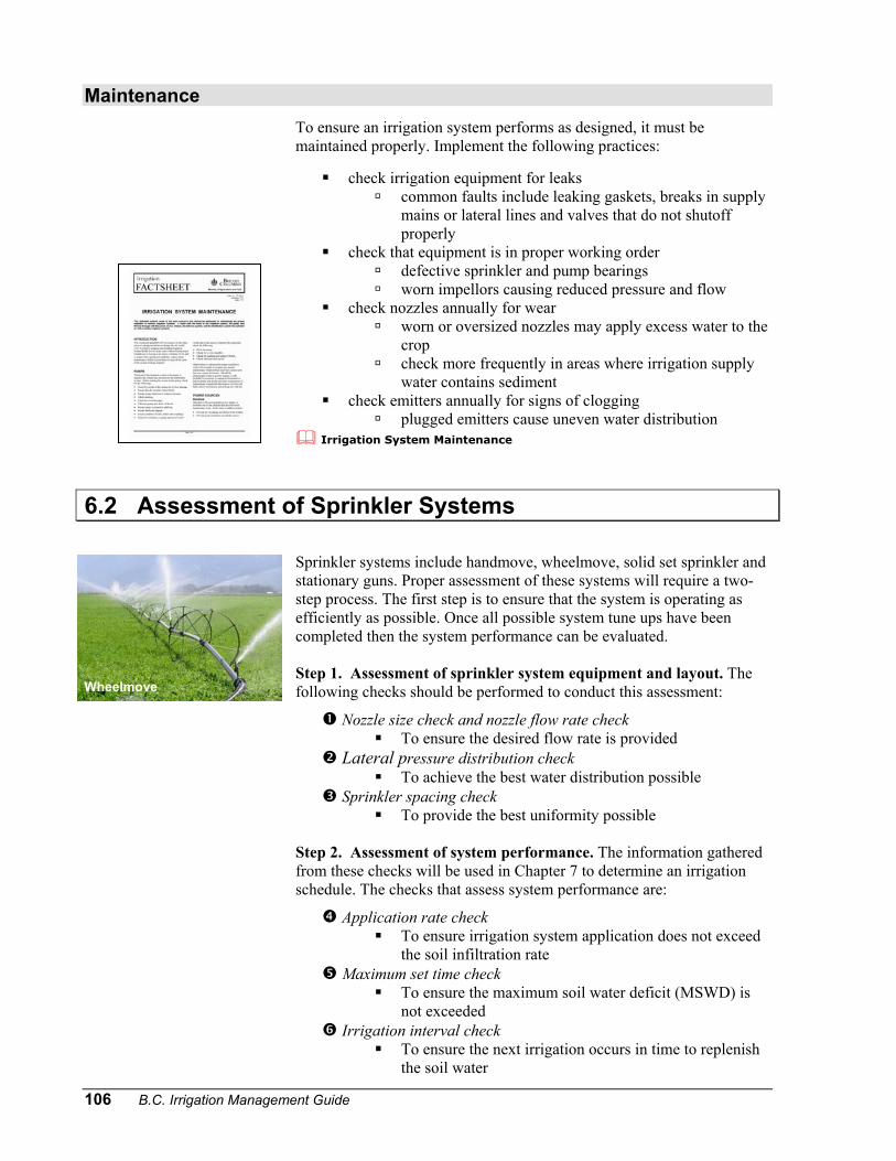
Maintenance To ensure an irrigation system performs as designed, it must be maintained properly. Implement the following practices:
check irrigation equipment for leaks common faults include leaking gaskets, breaks in supply
mains or lateral lines and valves that do not shutoff properly
check that equipment is in proper working order defective sprinkler and pump bearings
6.2
Wheel
B.C. Irrigation Management Guide
worn impellors causing reduced pressure and flow check nozzles annually for wear
worn or oversized nozzles may apply excess water to the crop
check more frequently in areas where irrigation supply water contains sediment
check emitters annually for signs of clogging plugged emitters cause uneven water distribution
Irrigation System Maintenance
Assessment of Sprinkler Systems Sprinkler systems include handmove, wheelmove, solid set sprinkler and stationary guns. Proper assessment of these systems will require a two-step process. The first step is to ensure that the system is operating as efficiently as possible. Once all possible system tune ups have been completed then the system performance can be evaluated. Step 1. Assessment of sprinkler system equipment and layout. The following checks should be performed to conduct this assessment:
Nozzle size check and nozzle flow rate check To ensure the desired flow rate is provided
Lateral pressure distribution check To achieve the best water distribution possible
Sprinkler spacing check To provide the best uniformity possible
Step 2. Assessment of system performance. The information gathered from these checks will be used in Chapter 7 to determine an irrigation schedule. The checks that assess system performance are:
Application rate check To ensure irrigation system application does not exceed
the soil infiltration rate Maximum set time check
To ensure the maximum soil water deficit (MSWD) is not exceeded
Irrigation interval check To ensure the next irrigation occurs in time to replenish
the soil water
move
Chapter 6 Irrigation System Assessment 107
Step 1. Assessment of Sprinkler System Equipment and Layout
Nozzle Size Check and Nozzle Flow Rate Check
The first check is to determine if all the nozzles are the same size or have worn due to wear. Over the years nozzles often get replaced with nozzles that are not matched to the original design. Wear and tear will also increase the nozzle opening so that more water may be applied than what the system was originally designed for. The nozzle size can be checked with a drill bit of the same size. If the drill bit does not fit snugly the nozzle should be replaced. Confirm that all nozzles on the lateral line are the same by either checking with a drill bit or reading the nozzle size stamped on the nozzle. If the nozzles are in good condition a nozzle flow rate check can be performed. Flow rates can be determined from sprinkler tables or measured directly. Measuring the flow rate on the farm provides the most accurate answer. Estimated values from tables provide guidance, but often do not reflect real farm conditions. Tables 6.2 can be used to determine the sprinkler flow rate using the nozzle size and operating pressure. A pressure gauge should be used to determine the pressure of the system while operating under normal conditions. Flow rates for various nozzle sizes, pressure and spacing can also be found in the B.C. Sprinkler Irrigation Manual. Appendix B provides conversions from imperial to metric units.
B.C. Sprinkler Irrigation Manual
Table 6.2 Sprinkler Discharge Rate Discharge Rate [US gpm]
Nozzle Diameter [inches] Pressure
[psi] 3/32 1/8 9/64 5/32 11/64 3/16 13/64 7/32
35 1.5 2.7 3.40 4.16 5.02 5.97 7.08 8.26
40 1.6 2.9 3.63 4.45 5.37 6.41 7.60 8.87
45 1.7 3.2 3.84 4.72 5.70 6.81 8.07 9.41
50 1.8 3.1 4.04 4.98 6.01 7.18 8.49 9.88
55 1.9 3.3 4.22 5.22 6.30 7.51 8.87 10.30
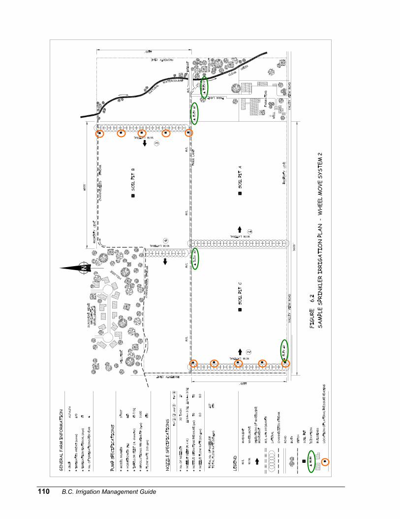
Assessment 6.1 provides a procedure for measuring the nozzle flow rate. The flow rate should be measured at a number of locations on the irrigation system. Figure 6.2 visually indicates where the system pressure and flow rate checks should be done. This is especially important if the irrigation lines run up and down a hill. Take measurements at high and low points along the lateral line.
108 B.C. Irrigation Management Guide
Assessment 6.1 Measuring Nozzle Flow Rate
Equipment Requirement Stop watch 5 gallon graduated pail
To create a graduated measuring pail, measure a gallon of water add a gallon at a time into the pail mark the top of the water line after each addition divide these marks into 4 equal segments to identify quarter gallons
Large hose – the end must be able to fit over the sprinkler nozzle
Select Measuring Points Select two laterals – one near the start of the irrigation system and the other near the end. Measure the nozzle flow rate at two locations along each lateral – one near the start and the
other near the end of the lateral If the lateral runs up and down a slope, take measurements at the highest and the lowest
point of the lateral.
Determine Sprinkler Flow Rate If there are two nozzles on the sprinkler head, measure each side separately and add the two flow rates together to find the total flow rate.
With the sprinkler operating, hold one end of the hose securely over the nozzle head ensuring that all of the flow is captured and flowing out of the end of the hose.
When ready, flip the end of the hose into the pail at the same time that the stop watch is started.
Time the flow for one minute. At one minute, flip the hose out of the pail. Estimate the amount of water in the pail by using the graduations on the side of the bucket
to determine the amount of water collected. The flow rate is the number of gallons collected within a minute (US gpm). For example, if
five gallons were collected in one minute, the flow rate is 5 US gpm. Repeat this process two or three times, and take the average of the flow rate
measurements.
Actions for Nozzle Size Check and Nozzle Flow Rate Check
If nozzles are worn or a lateral has mismatched nozzles:
Replace appropriate nozzles so that all nozzles on a lateral are identical in size. The nozzle selected should match the original system design.
Replace worn nozzles. Install flow control nozzles if the lateral has a significant elevation difference between the first
and last sprinkler.
Lateral Pressure Distribution Check
A lateral pressure distribution check provides good information to analyze system performance. If sprinklers along a lateral are operating at different pressures, the flow rate will also be different. A basic check procedure is explained here. A more in-depth check into friction losses and pressure requirements throughout the entire irrigation system is explained in Chapter 8. A significant change in pressure along an irrigation lateral line will cause flow rates to change, resulting in poor distribution of water over the field. Poor distribution results in uneven water application causing parts of the field being wetter or drier. Poor distribution often leads to the irrigation system being managed for the driest part of the field. Most of the field is
Chapter 6 Irrigation System Assessment 109
then over-irrigated and water lost to deep percolation or overland flow. The pressure difference caused by elevation differences may cause sprinklers along a lateral to have significant flow differences. If the lateral line cannot be run along a contour, a flow control nozzles should be used in the sprinkler instead of regular nozzles. Flow control nozzles maintain a constant flow from the sprinkler regardless of operating pressure.
Proper Usage of Flow Control Valves in Irrigation Systems Sprinkler pressure should be checked at the same locations as where the sprinkler flow rates are checked. Take pressure readings at:
the first sprinkler on the lateral the sprinklers approximately ¼ , ½ and ¾ of the distance along
the lateral (Figure 6.2 for wheelmove or handmove) the sprinkler at the end of the lateral
Figure 6.2 visually provides the locations where the system flow and pressure checks should be done for the sample irrigation system shown. A guide to the operating pressure range to achieve best efficiency for sprinklers at various flow rates is shown in Table 6.3. Table 6.3 Recommended Operating Pressure Range
for Sprinkler Systems
Flow Range [US gpm] Pressure Range [psi]
1 – 3 25 – 40
3 – 4 35 – 50
4 – 6 40 – 55
6 – 10 45 – 60
110 B.C. Irrigation Management Guide
Chapter 6 Irrigation System Assessment 111
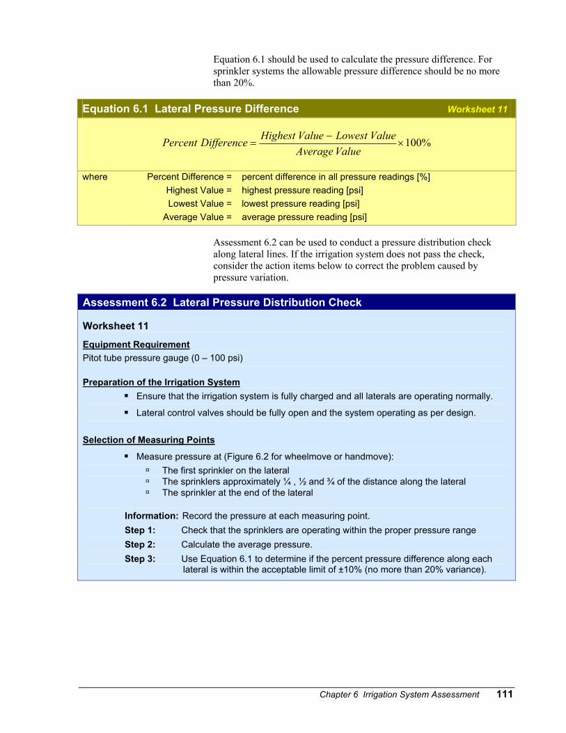
Equation 6.1 should be used to calculate the pressure difference. For sprinkler systems the allowable pressure difference should be no more than 20%.
Equation 6.1 Lateral Pressure Difference Worksheet 11
%100×−
=ValueAverage
ValueLowestValueHighestDifferencePercent
where Percent Difference = Highest Value = Lowest Value =
Average Value =
percent difference in all pressure readings [%] highest pressure reading [psi] lowest pressure reading [psi] average pressure reading [psi]
Assessment 6.2 can be used to conduct a pressure distribution check along lateral lines. If the irrigation system does not pass the check, consider the action items below to correct the problem caused by pressure variation.
Assessment 6.2 Lateral Pressure Distribution Check Worksheet 11 Equipment Requirement Pitot tube pressure gauge (0 – 100 psi)
Preparation of the Irrigation System Ensure that the irrigation system is fully charged and all laterals are operating normally.
Lateral control valves should be fully open and the system operating as per design.
Selection of Measuring Points
Measure pressure at (Figure 6.2 for wheelmove or handmove): The first sprinkler on the lateral The sprinklers approximately ¼ , ½ and ¾ of the distance along the lateral The sprinkler at the end of the lateral
Information: Record the pressure at each measuring point. Step 1: Check that the sprinklers are operating within the proper pressure range Step 2: Calculate the average pressure. Step 3: Use Equation 6.1 to determine if the percent pressure difference along each
lateral is within the acceptable limit of ±10% (no more than 20% variance).
112 B.C. Irrigation Management Guide
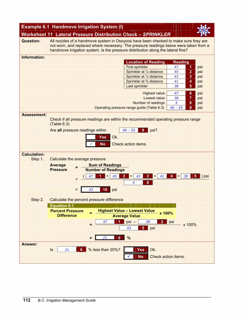
Example 6.1 Handmove Irrigation System (I)
Worksheet 11 Lateral Pressure Distribution Check – SPRINKLER
Question:
All nozzles of a handmove system in Osoyoos have been checked to make sure they are not worn, and replaced where necessary. The pressure readings below were taken from a handmove irrigation system. Is the pressure distribution along the lateral fine?
Information: Location of Reading Reading First sprinkler 47 1 psi Sprinkler at ¼ distance 45 2 psi Sprinkler at ½ distance 43 3 psi Sprinkler at ¾ distance 41 4 psi Last sprinkler 38 5 psi
Highest value 47 6 psi Lowest value 38 7 psi Number of readings 5 8 psi Operating pressure range guide (Table 6.3) 40 – 55 9 psi
Assessment:
Check if all pressure readings are within the recommended operating pressure range (Table 6.3)
Are all pressure readings within 40 – 55 9 psi?
Yes Ok.
No Check action items. Calculation: Step 1. Calculate the average pressure Sum of Readings
Average Pressure = Number of Readings
( 47 1 + 45 2 + 43 3 + 41 4 + 38 5 ) psi
= 5 8
= 43 10 psi Step 2. Calculate the percent pressure difference Equation 6.1 Highest Value – Lowest Value
Percent Pressure Difference = Average Value x 100%
47 1 psi – 38 2 psi
= 43 5 psi
x 100%
= 21 6 % Answer: Is 21 6 % less than 20%? Yes Ok.
No Check action items.
Chapter 6 Irrigation System Assessment 113
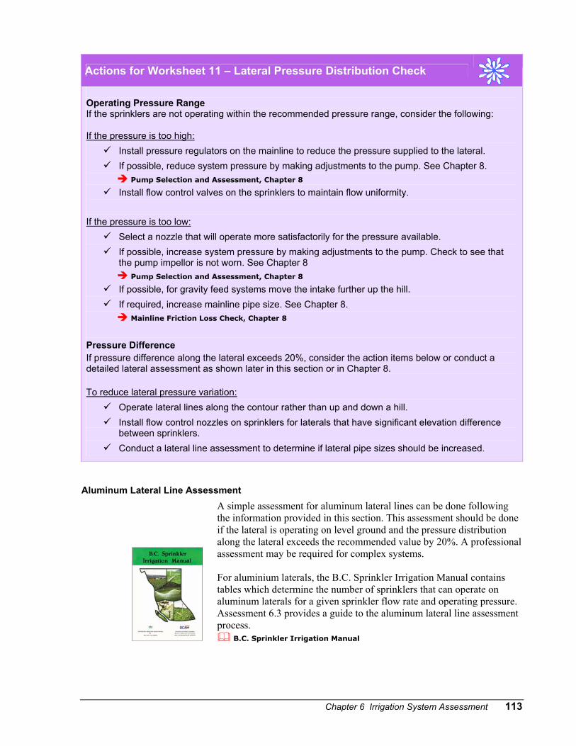
Actions for Worksheet 11 – Lateral Pressure Distribution Check
Operating Pressure Range If the sprinklers are not operating within the recommended pressure range, consider the following:
If the pressure is too high: Install pressure regulators on the mainline to reduce the pressure supplied to the lateral. If possible, reduce system pressure by making adjustments to the pump. See Chapter 8.
Pump Selection and Assessment, Chapter 8 Install flow control valves on the sprinklers to maintain flow uniformity.
If the pressure is too low:
Select a nozzle that will operate more satisfactorily for the pressure available. If possible, increase system pressure by making adjustments to the pump. Check to see that
the pump impellor is not worn. See Chapter 8 Pump Selection and Assessment, Chapter 8
If possible, for gravity feed systems move the intake further up the hill. If required, increase mainline pipe size. See Chapter 8.
Mainline Friction Loss Check, Chapter 8 Pressure Difference If pressure difference along the lateral exceeds 20%, consider the action items below or conduct a detailed lateral assessment as shown later in this section or in Chapter 8. To reduce lateral pressure variation:
Operate lateral lines along the contour rather than up and down a hill. Install flow control nozzles on sprinklers for laterals that have significant elevation difference
between sprinklers. Conduct a lateral line assessment to determine if lateral pipe sizes should be increased.
Aluminum Lateral Line Assessment A simple assessment for aluminum lateral lines can be done following the information provided in this section. This assessment should be done if the lateral is operating on level ground and the pressure distribution along the lateral exceeds the recommended value by 20%. A professional assessment may be required for complex systems. For aluminium laterals, the B.C. Sprinkler Irrigation Manual contains tables which determine the number of sprinklers that can operate on aluminum laterals for a given sprinkler flow rate and operating pressure. Assessment 6.3 provides a guide to the aluminum lateral line assessment process.
B.C. Sprinkler Irrigation Manual
114 B.C. Irrigation Management Guide
Assessment 6.3 Aluminum Lateral Line Assessment Worksheet 12
Use Tables 3.3 through 3.9 in the B.C. Sprinkler Irrigation Manual. Values in these tables are in imperial units. See Appendix B in this Guide for converting into metric units. The purpose of this assessment is to check if:
the nozzle sizes are appropriate for the desired flow rate the pressure at the beginning of the lateral matches the recommended value the number of sprinklers matches the recommended value
Information Determine the sprinkler spacing along the lateral and how far the lateral is moved for
each set. Determine the sprinkler flow rate and note the nozzle size. Determine the pressure at the first sprinkler, i.e., start of the lateral. Determine the lateral pipe size. If more than one pipe size is used for the lateral,
determine how much of each pipe is used. The tables provide options of having the pipe 100% one dimensional, with a split of 25 – 75% or 50 – 50%.
Determine the number of sprinklers operating on the lateral. Assessment
i. Find the appropriate table for the sprinkler spacing that matches the field conditions (Tables 3.3 to 3.9 in B.C. Sprinkler Irrigation Manual).
ii. Locate the sprinkler flow rate. iii. Check that the nozzle size and operating pressure are close to the recommended
value in the chart. iv. Under the column for “pressure at the start of the lateral”, check that the operating
pressure at the first sprinkler does not exceed the pressure shown in the table. v. Locate the pipe size(s) (with percentage split if appropriate). vi. Using the sprinkler flow rate and the pipe sizes, check that the number of sprinklers
operating on the lateral do not exceed the maximum number shown in the table for the lateral pipe size that is used.
Chapter 6 Irrigation System Assessment 115
Example 6.2 Handmove Irrigation System (II)
Worksheet 12 Wheelmove or Handmove Lateral Line Assessment
Question:
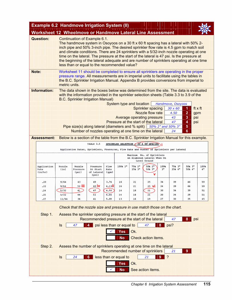
Continuation of Example 6.1. The handmove system in Osoyoos on a 30 ft x 60 ft spacing has a lateral with 50% 2-inch pipe and 50% 3-inch pipe. The desired sprinkler flow rate is 4.5 gpm to match soil and climate conditions. There are 24 sprinklers with a 5/32-inch nozzle operating at one time on the lateral. The pressure at the start of the lateral is 47 psi. Is the pressure at the beginning of the lateral adequate and are number of sprinklers operating at one time less than or equal to the recommended value?
Note:
Worksheet 11 should be completed to ensure all sprinklers are operating in the proper pressure range. All measurements are in imperial units to facilitate using the tables in the B.C. Sprinkler Irrigation Manual. Appendix B provides conversions from imperial to metric units.
Information:
The data shown in the boxes below was determined from the site. The data is evaluated with the information provided in the sprinkler selection sheets (Table 3.3 to 3.9 of the B.C. Sprinkler Irrigation Manual)
System type and location Handmove, Osoyoos Sprinkler spacing 30 x 60 1 ft x ft Nozzle flow rate 4.50 2 gpm Average operating pressure 43 3 psi Pressure at the start of the lateral 47 4 psi Pipe size(s) along lateral (diameters and % split) 50% 2” and 50% 3” 5 Number of nozzles operating at one time on the lateral 24 6
Assessment: Below is a section of the table from the B.C. Sprinkler Irrigation Manual for this example. Check that the nozzle size and pressure in use match those on the chart.
Step 1. Assess the sprinkler operating pressure at the start of the lateral Recommended pressure at the start of the lateral 47 8 psi Is 47 4 psi less than or equal to 47 8 psi?
Yes Ok. No Check action items. Step 2. Assess the number of sprinklers operating at one time on the lateral Recommended number of sprinklers 21 9 Is 24 6 less than or equal to 21 9 ?
Yes Ok. No See action items.
vi
v
i
iv iiiii
116 B.C. Irrigation Management Guide
Actions for Worksheet 12 – Aluminum Lateral Line Assessment
Problems with aluminum laterals can be resolved by shortening the lateral line, using bigger pipe or installing smaller nozzles. The action to take depends on following:
Scenario 1. Pressure at start of lateral is lower than shown in chart Okay if all of the sprinklers are operating within the recommended pressure range
and providing the required flow. This will usually be the case with short laterals.
Increase pressure if the sprinklers at the end of the line are not operating at the correct pressure. Ensure that required pressure range along lateral is not exceeded.
Scenario 2. Pressure at start of lateral is higher than shown in chart First, reduce the pressure at start of lateral to the recommended pressure shown in
chart. Then, check that the last sprinkler on the line is still operating within the recommended pressure.
If sprinkler operating pressure variation exceeds 20%, the lateral pipe size should be increased or the number of sprinklers operating on the lateral reduced.
Scenario 3. The number of sprinkler operating on the lateral is less than shown on chart Okay. The lateral pipe is just oversized but pressure uniformity will be good.
Scenario 4. The number of sprinkler operating on the lateral exceeds value on chart
Reduce the number of sprinklers on the lateral or increase the pipe size that will accommodate the number of sprinklers operating on the lateral.
PVC Lateral Line Assessment Conducting an assessment on a PVC lateral is more complex than aluminum pipe, and will require friction loss charts to complete the assessment. Friction loss along the lateral does not usually affect total dynamic head significantly but is important from a system application uniformity perspective. To assess the friction loss of a PVC lateral, Assessment 6.4 should be followed. Friction loss tables in Appendix B of the B.C. Sprinkler Irrigation Manual can be used.
Chapter 6 Irrigation System Assessment 117
Assessment 6.4 PVC Lateral Line Assessment Worksheet 13 Use Appendix B in the B.C. Sprinkler Irrigation Manual. Values in these tables are in imperial units. See Appendix B in this Guide for converting into metric units. Information
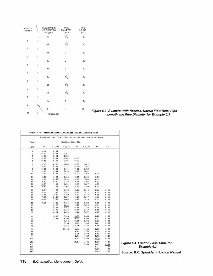
Figure 6.3 illustrates how to gather the following information for a solid set lateral. Determine the maximum total friction loss allowed (20% of the sprinkler operating
pressure. Determine the nozzle flow rate. Fill in the information section of the worksheet with the
total flow rate for each section of the pipe. For example, the first section of the pipe must carry enough water (flow) to feed all the sprinklers on the line. The last section of pipe needs to only carry enough water to feed the last sprinkler.
Write down the corresponding pipe section diameter for each flow rate. Write down the pipe length between the sprinklers. Go to the friction loss tables in Appendix B of the B.C. Sprinkler Irrigation Manual for the
type of pipe being used (Figure 6.4 shows a sample table to be used in Example 6.3): Locate the flow rate at the start of the lateral. Choose a pipe size along the row with this flow rate and with friction loss values
above the cut-off line as friction losses below the line are too high. Repeat for all pipe sections.
Assessment Add up all the friction losses, and add 10% of the total as miscellaneous losses. Check that the total friction loss does not exceed 20% of the sprinkler operating pressure.
If there is severe elevation changes along the lateral the elevation change should be included a part of the allowable 20% variation.
118 B.C. Irrigation Management Guide
F
igure 6.3 A Lateral with Nozzles, Nozzle Flow Rate, PipeLength and Pipe Diameter for Example 6.3
Figure 6.4 Friction Loss Table for Example 6.3
Source: B.C. Sprinkler Irrigation Manual
Chapter 6 Irrigation System Assessment 119
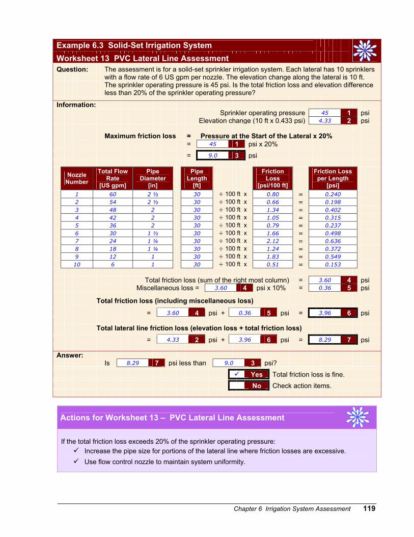
Example 6.3 Solid-Set Irrigation System
Worksheet 13 PVC Lateral Line Assessment
Question:
The assessment is for a solid-set sprinkler irrigation system. Each lateral has 10 sprinklers with a flow rate of 6 US gpm per nozzle. The elevation change along the lateral is 10 ft. The sprinkler operating pressure is 45 psi. Is the total friction loss and elevation difference less than 20% of the sprinkler operating pressure?
Information: Sprinkler operating pressure 45 1 psi Elevation change (10 ft x 0.433 psi) 4.33 2 psi Maximum friction loss = Pressure at the Start of the Lateral x 20% = 45 1 psi x 20%
= 9.0 3 psi
Nozzle Number
Total Flow Rate
[US gpm]
Pipe Diameter
[in]
Pipe Length
[ft]
Friction Loss
[psi/100 ft]
Friction Loss per Length
[psi] 1 60 2 ½ 30 ÷ 100 ft x 0.80 = 0.240 2 54 2 ½ 30 ÷ 100 ft x 0.66 = 0.198 3 48 2 30 ÷ 100 ft x 1.34 = 0.402 4 42 2 30 ÷ 100 ft x 1.05 = 0.315 5 36 2 30 ÷ 100 ft x 0.79 = 0.237 6 30 1 ½ 30 ÷ 100 ft x 1.66 = 0.498 7 24 1 ¼ 30 ÷ 100 ft x 2.12 = 0.636 8 18 1 ¼ 30 ÷ 100 ft x 1.24 = 0.372 9 12 1 30 ÷ 100 ft x 1.83 = 0.549 10 6 1 30 ÷ 100 ft x 0.51 = 0.153
Total friction loss (sum of the right most column) = 3.60 4 psi Miscellaneous loss = 3.60 4 psi x 10% = 0.36 5 psi
Total friction loss (including miscellaneous loss)
= 3.60 4 psi + 0.36 5 psi = 3.96 6 psi Total lateral line friction loss (elevation loss + total friction loss)
= 4.33 2 psi + 3.96 6 psi = 8.29 7 psi Answer: Is 8.29 7 psi less than 9.0 3 psi?
Yes Total friction loss is fine. No Check action items.
Actions for Worksheet 13 – PVC Lateral Line Assessment
If the total friction loss exceeds 20% of the sprinkler operating pressure:
Increase the pipe size for portions of the lateral line where friction losses are excessive. Use flow control nozzle to maintain system uniformity.
120 B.C. Irrigation Management Guide
Sprinkler Spacing Check
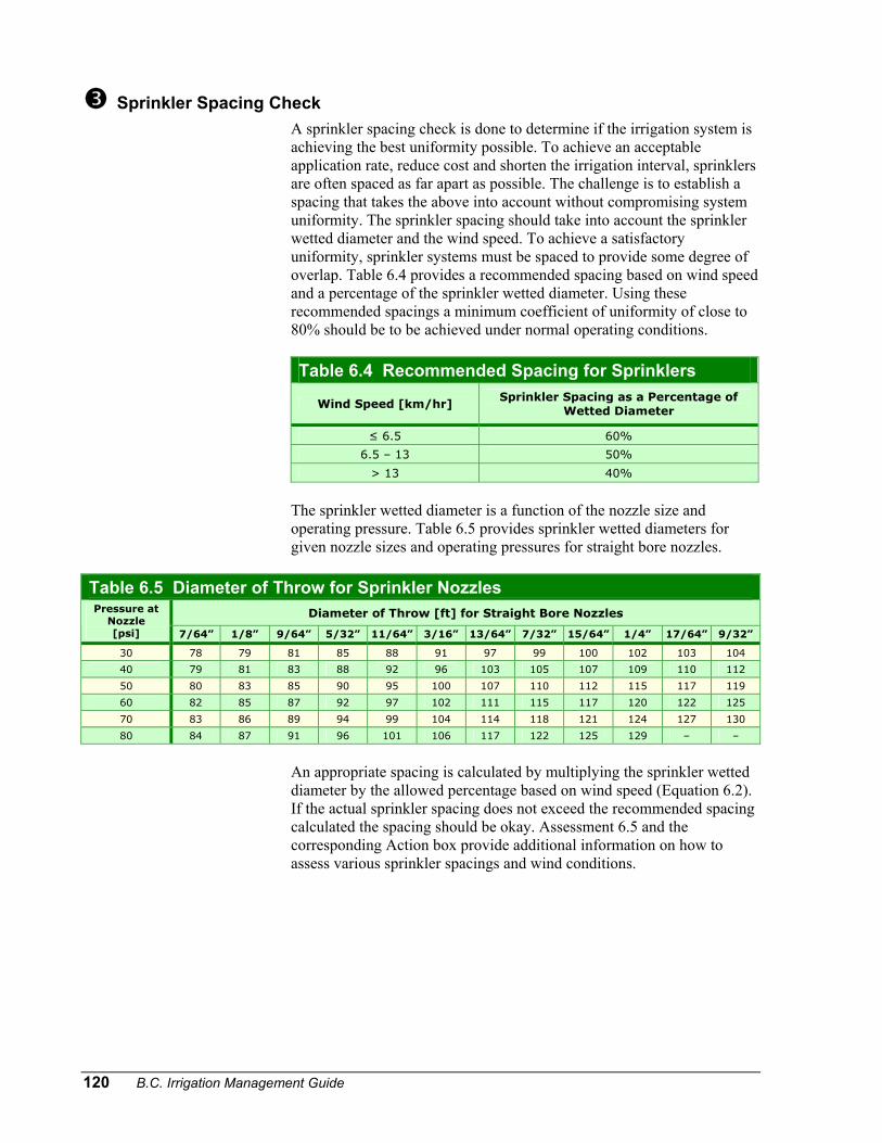
A sprinkler spacing check is done to determine if the irrigation system is achieving the best uniformity possible. To achieve an acceptable application rate, reduce cost and shorten the irrigation interval, sprinklers are often spaced as far apart as possible. The challenge is to establish a spacing that takes the above into account without compromising system uniformity. The sprinkler spacing should take into account the sprinkler wetted diameter and the wind speed. To achieve a satisfactory uniformity, sprinkler systems must be spaced to provide some degree of overlap. Table 6.4 provides a recommended spacing based on wind speed and a percentage of the sprinkler wetted diameter. Using these recommended spacings a minimum coefficient of uniformity of close to 80% should be to be achieved under normal operating conditions. Table 6.4 Recommended Spacing for Sprinklers
Wind Speed [km/hr] Sprinkler Spacing as a Percentage of
Wetted Diameter
≤ 6.5 60%
6.5 – 13 50%
> 13 40%
The sprinkler wetted diameter is a function of the nozzle size and operating pressure. Table 6.5 provides sprinkler wetted diameters for given nozzle sizes and operating pressures for straight bore nozzles.
Table 6.5 Diameter of Throw for Sprinkler Nozzles Diameter of Throw [ft] for Straight Bore Nozzles Pressure at
Nozzle [psi] 7/64” 1/8” 9/64” 5/32” 11/64” 3/16” 13/64” 7/32” 15/64” 1/4” 17/64” 9/32”
30 78 79 81 85 88 91 97 99 100 102 103 104
40 79 81 83 88 92 96 103 105 107 109 110 112
50 80 83 85 90 95 100 107 110 112 115 117 119
60 82 85 87 92 97 102 111 115 117 120 122 125
70 83 86 89 94 99 104 114 118 121 124 127 130
80 84 87 91 96 101 106 117 122 125 129 – –
An appropriate spacing is calculated by multiplying the sprinkler wetted diameter by the allowed percentage based on wind speed (Equation 6.2). If the actual sprinkler spacing does not exceed the recommended spacing calculated the spacing should be okay. Assessment 6.5 and the corresponding Action box provide additional information on how to assess various sprinkler spacings and wind conditions.
Chapter 6 Irrigation System Assessment 121
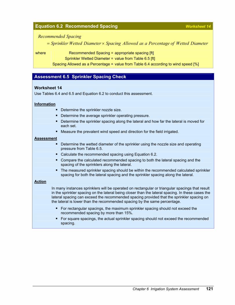
Equation 6.2 Recommended Spacing Worksheet 14
DiameterWettedofPercentageaasAllowedSpacingDiameterWettedSprinklerSpacingecommendedR
×=
where Recommended Spacing =Sprinkler Wetted Diameter =
Spacing Allowed as a Percentage =
appropriate spacing [ft] value from Table 6.5 [ft] value from Table 6.4 according to wind speed [%]
Assessment 6.5 Sprinkler Spacing Check Worksheet 14 Use Tables 6.4 and 6.5 and Equation 6.2 to conduct this assessment. Information
Determine the sprinkler nozzle size. Determine the average sprinkler operating pressure. Determine the sprinkler spacing along the lateral and how far the lateral is moved for
each set. Measure the prevalent wind speed and direction for the field irrigated.
Assessment Determine the wetted diameter of the sprinkler using the nozzle size and operating
pressure from Table 6.5. Calculate the recommended spacing using Equation 6.2. Compare the calculated recommended spacing to both the lateral spacing and the
spacing of the sprinklers along the lateral. The measured sprinkler spacing should be within the recommended calculated sprinkler
spacing for both the lateral spacing and the sprinkler spacing along the lateral.
Action
In many instances sprinklers will be operated on rectangular or triangular spacings that result in the sprinkler spacing on the lateral being closer than the lateral spacing. In these cases the lateral spacing can exceed the recommended spacing provided that the sprinkler spacing on the lateral is lower than the recommended spacing by the same percentage.
For rectangular spacings, the maximum sprinkler spacing should not exceed the recommended spacing by more than 15%.
For square spacings, the actual sprinkler spacing should not exceed the recommended spacing.
122 B.C. Irrigation Management Guide
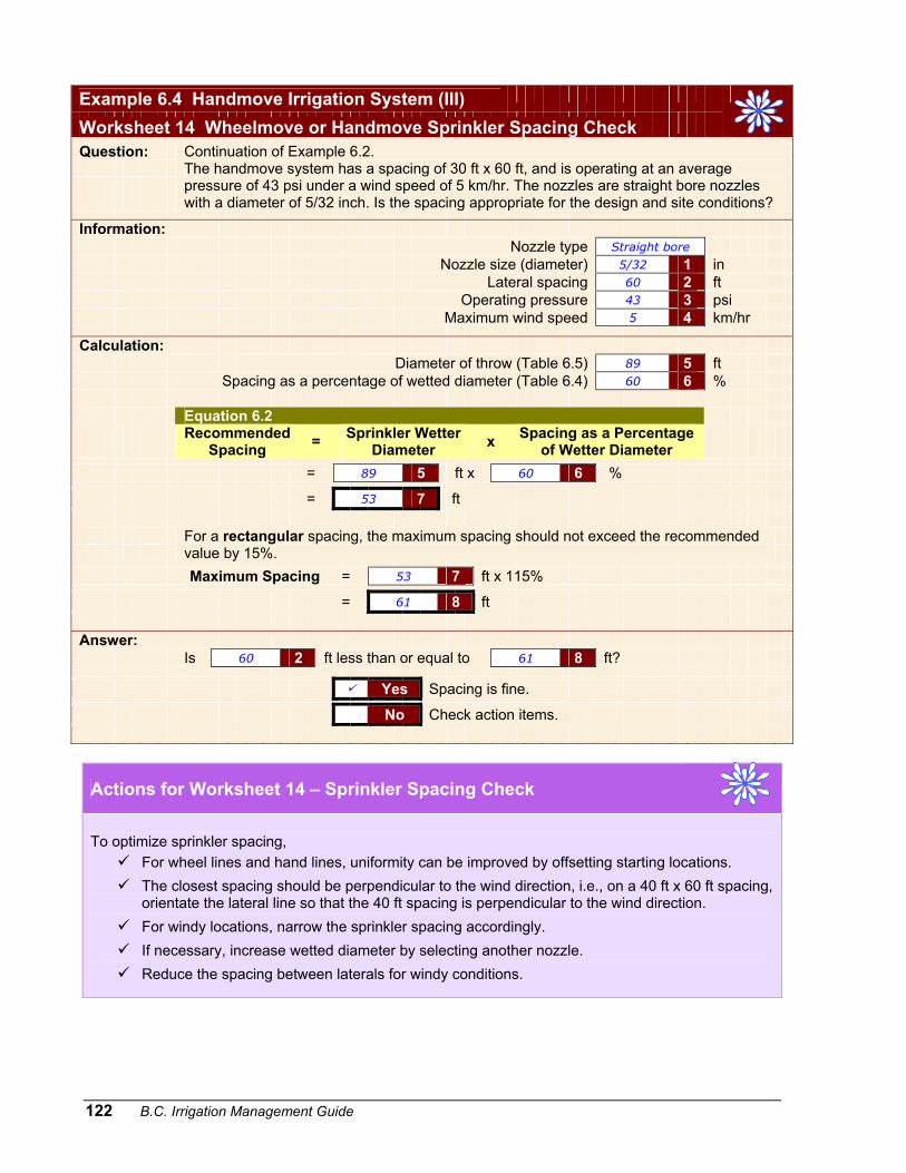
Example 6.4 Handmove Irrigation System (III)
Worksheet 14 Wheelmove or Handmove Sprinkler Spacing Check
Question:
Continuation of Example 6.2. The handmove system has a spacing of 30 ft x 60 ft, and is operating at an average pressure of 43 psi under a wind speed of 5 km/hr. The nozzles are straight bore nozzles with a diameter of 5/32 inch. Is the spacing appropriate for the design and site conditions?
Information: Nozzle type Straight bore Nozzle size (diameter) 5/32 1 in Lateral spacing 60 2 ft Operating pressure 43 3 psi Maximum wind speed 5 4 km/hr
Calculation: Diameter of throw (Table 6.5) 89 5 ft Spacing as a percentage of wetted diameter (Table 6.4) 60 6 % Equation 6.2
Recommended Spacing = Sprinkler Wetter
Diameter x Spacing as a Percentage of Wetter Diameter
= 89 5 ft x 60 6 %
= 53 7 ft
For a rectangular spacing, the maximum spacing should not exceed the recommended value by 15%.
Maximum Spacing = 53 7 ft x 115%
= 61 8 ft Answer: Is 60 2 ft less than or equal to 61 8 ft?
Yes Spacing is fine.
No Check action items.
Actions for Worksheet 14 – Sprinkler Spacing Check
To optimize sprinkler spacing,
For wheel lines and hand lines, uniformity can be improved by offsetting starting locations. The closest spacing should be perpendicular to the wind direction, i.e., on a 40 ft x 60 ft spacing,
orientate the lateral line so that the 40 ft spacing is perpendicular to the wind direction. For windy locations, narrow the sprinkler spacing accordingly. If necessary, increase wetted diameter by selecting another nozzle. Reduce the spacing between laterals for windy conditions.
Chapter 6 Irrigation System Assessment 123
Step 2. Assessment of Sprinkler System Performance The system performance assessment can only be done once the system equipment and layout assessment has been completed in Step 1. Conducting a system performance check is not of much value unless the system is operating as effectively as possible. The following system performance checks will be used in Chapter 7 to prepare an irrigation schedule.
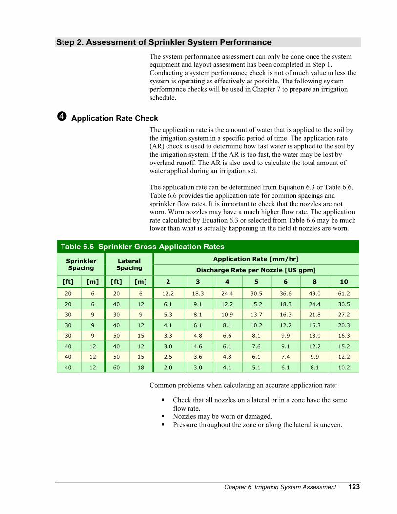
Application Rate Check
The application rate is the amount of water that is applied to the soil by the irrigation system in a specific period of time. The application rate (AR) check is used to determine how fast water is applied to the soil by the irrigation system. If the AR is too fast, the water may be lost by overland runoff. The AR is also used to calculate the total amount of water applied during an irrigation set. The application rate can be determined from Equation 6.3 or Table 6.6. Table 6.6 provides the application rate for common spacings and sprinkler flow rates. It is important to check that the nozzles are not worn. Worn nozzles may have a much higher flow rate. The application rate calculated by Equation 6.3 or selected from Table 6.6 may be much lower than what is actually happening in the field if nozzles are worn.
Table 6.6 Sprinkler Gross Application Rates Application Rate [mm/hr] Sprinkler
Spacing Lateral Spacing Discharge Rate per Nozzle [US gpm]
[ft] [m] [ft] [m] 2 3 4 5 6 8 10
20 6 20 6 12.2 18.3 24.4 30.5 36.6 49.0 61.2
20 6 40 12 6.1 9.1 12.2 15.2 18.3 24.4 30.5
30 9 30 9 5.3 8.1 10.9 13.7 16.3 21.8 27.2
30 9 40 12 4.1 6.1 8.1 10.2 12.2 16.3 20.3
30 9 50 15 3.3 4.8 6.6 8.1 9.9 13.0 16.3
40 12 40 12 3.0 4.6 6.1 7.6 9.1 12.2 15.2
40 12 50 15 2.5 3.6 4.8 6.1 7.4 9.9 12.2
40 12 60 18 2.0 3.0 4.1 5.1 6.1 8.1 10.2
Common problems when calculating an accurate application rate:
Check that all nozzles on a lateral or in a zone have the same flow rate.
Nozzles may be worn or damaged. Pressure throughout the zone or along the lateral is uneven.
124 B.C. Irrigation Management Guide
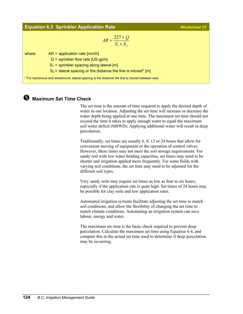
Equation 6.3 Sprinkler Application Rate Worksheet 15
21
227SSQAR
××
=
where
AR = Q = S1 = S2 =
application rate [mm/h] sprinkler flow rate [US gpm] sprinkler spacing along lateral [m] lateral spacing or the distance the line is moved* [m]
* For handmove and wheelmove, lateral spacing is the distance the line is moved between sets.
Maximum Set Time Check The set time is the amount of time required to apply the desired depth of water in one location. Adjusting the set time will increase or decrease the water depth being applied at one time. The maximum set time should not exceed the time it takes to apply enough water to equal the maximum soil water deficit (MSWD). Applying additional water will result in deep percolation. Traditionally, set times are usually 6, 8, 12 or 24 hours that allow for convenient moving of equipment or the operation of control valves. However, these times may not meet the soil storage requirements. For sandy soil with low water holding capacities, set times may need to be shorter and irrigation applied more frequently. For some fields with varying soil conditions, the set time may need to be adjusted for the different soil types. Very sandy soils may require set times as low as four to six hours, especially if the application rate is quite high. Set times of 24 hours may be possible for clay soils and low application rates. Automated irrigation systems facilitate adjusting the set time to match soil conditions, and allow the flexibility of changing the set time to match climate conditions. Automating an irrigation system can save labour, energy and water. The maximum set time is the basic check required to prevent deep percolation. Calculate the maximum set time using Equation 6.4, and compare this to the actual set time used to determine if deep percolation may be occurring.
Chapter 6 Irrigation System Assessment 125
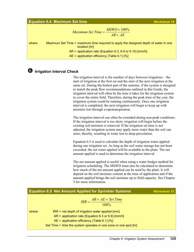
Equation 6.4 Maximum Set time Worksheet 15
AEARMSWDTimeSetMaximum
××
=%100
where
Maximum Set Time =
AR = AE =
maximum time required to apply the designed depth of water in one location [hr] application rate (Equation 6.3, 6.9 or 6.10) [mm/h] application efficiency (Table 6.1) [%]
Irrigation Interval Check
The irrigation interval is the number of days between irrigations – the start of irrigation at the first set and the start of the next irrigation at the same set. During the hottest part of the summer, if the system is designed to match the peak flow recommendations outlined in this Guide, the irrigation interval will often be the time it takes for the irrigation system to cover the entire field. Therefore, during the peak time of the year, the irrigation system could be running continuously. Once one irrigation interval is completed, the next irrigation will begin to keep up with moisture lost through evapotranspiration. The irrigation interval can often be extended during non-peak conditions. If the irrigation interval is too short, irrigation will begin before the existing soil moisture is removed. If the irrigation set time is not adjusted, the irrigation system may apply more water than the soil can store; thereby, resulting in water lost to deep percolation. Equation 6.5 is used to calculate the depth of irrigation water applied during one irrigation set. As long as the soil water storage has not been exceeded, the net water applied will be available to the plant. The net amount applied is used to determine the irrigation interval. The net amount applied is useful when using a water budget method for irrigation scheduling. The MSWD must also be calculated to determine how much of the net amount applied can be used by the plant. It will depend on the soil moisture content at the time of application and if the amount applied brings the soil moisture up to field capacity. See Chapter 5 for more information.
Equation 6.5 Net Amount Applied for Sprinkler Systems Worksheet 15
%100TimeSetAEARIRR ××
=
where
IRR = AR = AE =
Set Time =
net depth of irrigation water applied [mm] application rate (Equation 6.3 or 6.9) [mm/h] application efficiency (Table 6.1) [%] time the system operates in one zone or one spot [hr]
126 B.C. Irrigation Management Guide
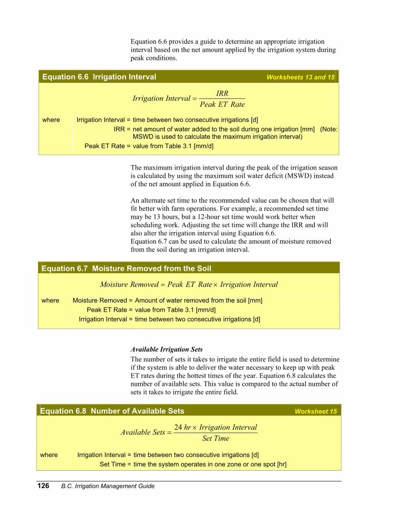
Equation 6.6 provides a guide to determine an appropriate irrigation interval based on the net amount applied by the irrigation system during peak conditions.
Equation 6.6 Irrigation Interval Worksheets 13 and 15
RateETPeakIRRIntervalIrrigation =
where
Irrigation Interval = IRR =
Peak ET Rate =
time between two consecutive irrigations [d] net amount of water added to the soil during one irrigation [mm] (Note: MSWD is used to calculate the maximum irrigation interval) value from Table 3.1 [mm/d]
The maximum irrigation interval during the peak of the irrigation season is calculated by using the maximum soil water deficit (MSWD) instead of the net amount applied in Equation 6.6. An alternate set time to the recommended value can be chosen that will fit better with farm operations. For example, a recommended set time may be 13 hours, but a 12-hour set time would work better when scheduling work. Adjusting the set time will change the IRR and will also alter the irrigation interval using Equation 6.6. Equation 6.7 can be used to calculate the amount of moisture removed from the soil during an irrigation interval.
Equation 6.7 Moisture Removed from the Soil
IntervalIrrigationRateETPeakemovedRMoisture ×=
where
Moisture Removed = Peak ET Rate =
Irrigation Interval =
Amount of water removed from the soil [mm] value from Table 3.1 [mm/d] time between two consecutive irrigations [d]
Available Irrigation Sets The number of sets it takes to irrigate the entire field is used to determine if the system is able to deliver the water necessary to keep up with peak ET rates during the hottest times of the year. Equation 6.8 calculates the number of available sets. This value is compared to the actual number of sets it takes to irrigate the entire field.
Equation 6.8 Number of Available Sets Worksheet 15
TimeSetIntervalIrrigationhrSetsAvailable ×
=24
where
Irrigation Interval = Set Time =
time between two consecutive irrigations [d] time the system operates in one zone or one spot [hr]
Chapter 6 Irrigation System Assessment 127
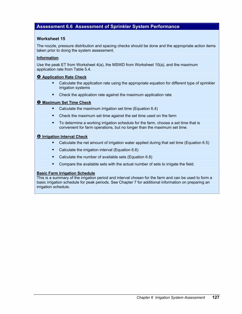
Assessment 6.6 Assessment of Sprinkler System Performance Worksheet 15 The nozzle, pressure distribution and spacing checks should be done and the appropriate action items taken prior to doing the system assessment.
Information
Use the peak ET from Worksheet 4(a), the MSWD from Worksheet 10(a), and the maximum application rate from Table 5.4.
Application Rate Check Calculate the application rate using the appropriate equation for different type of sprinkler
irrigation systems
Check the application rate against the maximum application rate
Maximum Set Time Check Calculate the maximum irrigation set time (Equation 6.4)
Check the maximum set time against the set time used on the farm
To determine a working irrigation schedule for the farm, choose a set time that is convenient for farm operations, but no longer than the maximum set time.
Irrigation Interval Check Calculate the net amount of irrigation water applied during that set time (Equation 6.5)
Calculate the irrigation interval (Equation 6.6)
Calculate the number of available sets (Equation 6.8)
Compare the available sets with the actual number of sets to irrigate the field.
Basic Farm Irrigation Schedule This is a summary of the irrigation period and interval chosen for the farm and can be used to form a basic irrigation schedule for peak periods. See Chapter 7 for additional information on preparing an irrigation schedule.
128 B.C. Irrigation Management Guide
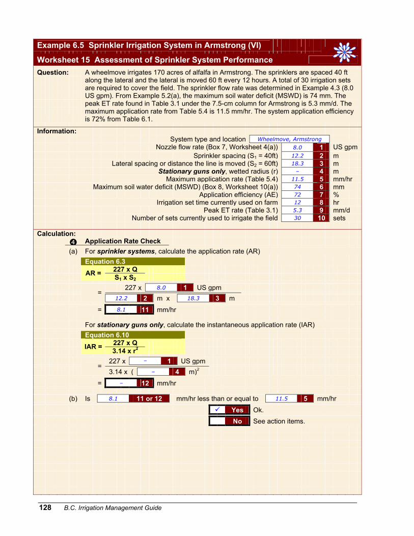
Example 6.5 Sprinkler Irrigation System in Armstrong (VI)
Worksheet 15 Assessment of Sprinkler System Performance
Question:
A wheelmove irrigates 170 acres of alfalfa in Armstrong. The sprinklers are spaced 40 ft along the lateral and the lateral is moved 60 ft every 12 hours. A total of 30 irrigation sets are required to cover the field. The sprinkler flow rate was determined in Example 4.3 (8.0 US gpm). From Example 5.2(a), the maximum soil water deficit (MSWD) is 74 mm. The peak ET rate found in Table 3.1 under the 7.5-cm column for Armstrong is 5.3 mm/d. The maximum application rate from Table 5.4 is 11.5 mm/hr. The system application efficiency is 72% from Table 6.1.
Information: System type and location Wheelmove, Armstrong
Nozzle flow rate (Box 7, Worksheet 4(a)) 8.0 1 US gpm Sprinkler spacing (S1 = 40ft) 12.2 2 m Lateral spacing or distance the line is moved (S2 = 60ft) 18.3 3 m Stationary guns only, wetted radius (r) – 4 m Maximum application rate (Table 5.4) 11.5 5 mm/hr Maximum soil water deficit (MSWD) (Box 8, Worksheet 10(a)) 74 6 mm Application efficiency (AE) 72 7 % Irrigation set time currently used on farm 12 8 hr Peak ET rate (Table 3.1) 5.3 9 mm/d Number of sets currently used to irrigate the field 30 10 sets Calculation: Application Rate Check (a) For sprinkler systems, calculate the application rate (AR) Equation 6.3 227 x Q AR = S1 x S2 227 x 8.0 1 US gpm
= 12.2 2 m x 18.3 3 m
= 8.1 11 mm/hr For stationary guns only, calculate the instantaneous application rate (IAR) Equation 6.10 227 x Q IAR = 3.14 x r2 227 x – 1 US gpm
= 3.14 x ( – 4 m)2
= – 12 mm/hr (b) Is 8.1 11 or 12 mm/hr less than or equal to 11.5 5 mm/hr
Yes Ok. No See action items.
Chapter 6 Irrigation System Assessment 129
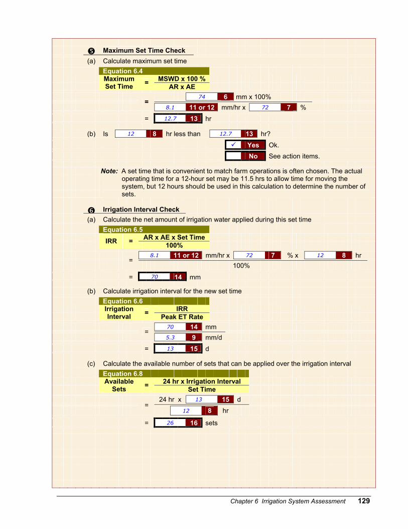
Maximum Set Time Check (a) Calculate maximum set time Equation 6.4 MSWD x 100 %
Maximum Set Time = AR x AE
74 6 mm x 100%
= 8.1 11 or 12 mm/hr x 72 7 %
= 12.7 13 hr (b) Is 12 8 hr less than 12.7 13 hr?
Yes Ok. No See action items.
Note: A set time that is convenient to match farm operations is often chosen. The actual operating time for a 12-hour set may be 11.5 hrs to allow time for moving the system, but 12 hours should be used in this calculation to determine the number of sets.
Irrigation Interval Check (a) Calculate the net amount of irrigation water applied during this set time Equation 6.5 AR x AE x Set Time IRR = 100% 8.1 11 or 12 mm/hr x 72 7 % x 12 8 hr
= 100%
= 70 14 mm (b) Calculate irrigation interval for the new set time Equation 6.6 IRR
Irrigation Interval = Peak ET Rate
70 14 mm
= 5.3 9 mm/d
= 13 15 d (c) Calculate the available number of sets that can be applied over the irrigation interval Equation 6.8 24 hr x Irrigation Interval
Available Sets = Set Time
24 hr x 13 15 d
= 12 8 hr
= 26 16 sets
130 B.C. Irrigation Management Guide
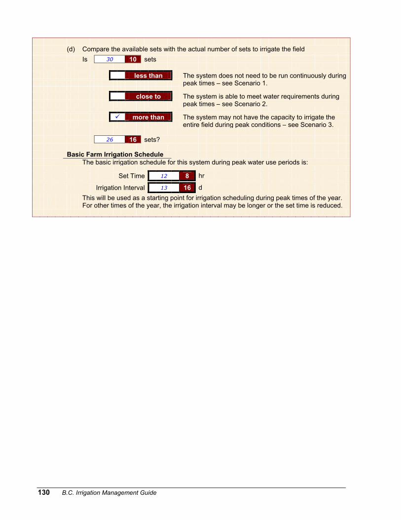
(d) Compare the available sets with the actual number of sets to irrigate the field Is 30 10 sets less than
The system does not need to be run continuously during peak times – see Scenario 1.
close to
The system is able to meet water requirements during peak times – see Scenario 2.
more than
The system may not have the capacity to irrigate the entire field during peak conditions – see Scenario 3.
26 16 sets? Basic Farm Irrigation Schedule The basic irrigation schedule for this system during peak water use periods is:
Set Time 12 8 hr
Irrigation Interval 13 16 d
This will be used as a starting point for irrigation scheduling during peak times of the year. For other times of the year, the irrigation interval may be longer or the set time is reduced.
Chapter 6 Irrigation System Assessment 131
Actions for Worksheet 15 – Assessment of Sprinkler System Performance
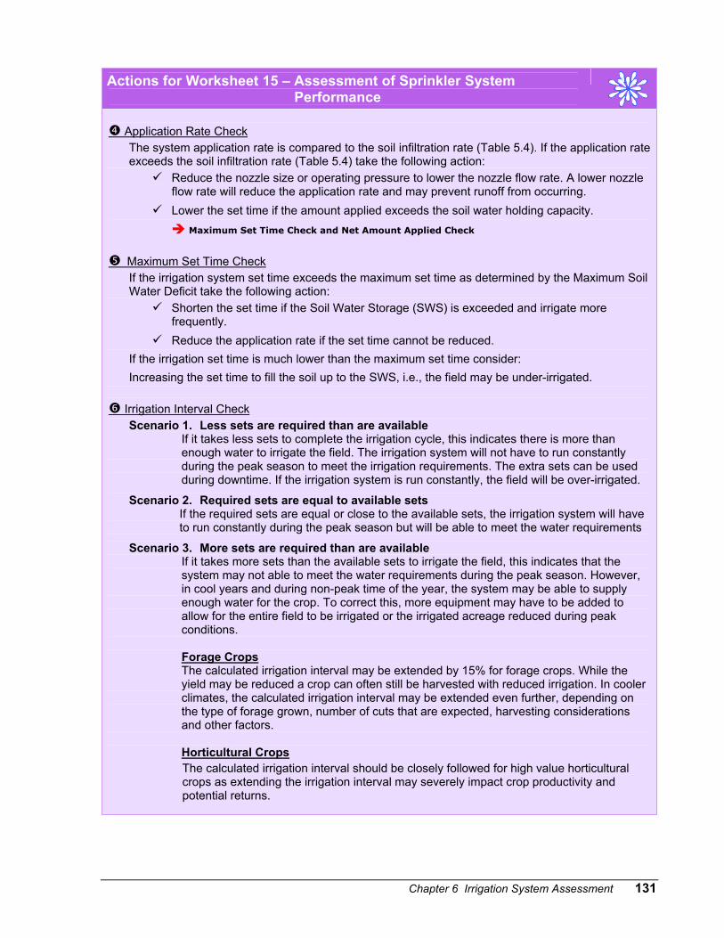
Application Rate Check
The system application rate is compared to the soil infiltration rate (Table 5.4). If the application rate exceeds the soil infiltration rate (Table 5.4) take the following action:
Reduce the nozzle size or operating pressure to lower the nozzle flow rate. A lower nozzle flow rate will reduce the application rate and may prevent runoff from occurring.
Lower the set time if the amount applied exceeds the soil water holding capacity. Maximum Set Time Check and Net Amount Applied Check
Maximum Set Time Check If the irrigation system set time exceeds the maximum set time as determined by the Maximum Soil Water Deficit take the following action:
Shorten the set time if the Soil Water Storage (SWS) is exceeded and irrigate more frequently.
Reduce the application rate if the set time cannot be reduced. If the irrigation set time is much lower than the maximum set time consider: Increasing the set time to fill the soil up to the SWS, i.e., the field may be under-irrigated.
Irrigation Interval Check Scenario 1. Less sets are required than are available
If it takes less sets to complete the irrigation cycle, this indicates there is more than enough water to irrigate the field. The irrigation system will not have to run constantly during the peak season to meet the irrigation requirements. The extra sets can be used during downtime. If the irrigation system is run constantly, the field will be over-irrigated.
Scenario 2. Required sets are equal to available sets If the required sets are equal or close to the available sets, the irrigation system will have to run constantly during the peak season but will be able to meet the water requirements
Scenario 3. More sets are required than are available If it takes more sets than the available sets to irrigate the field, this indicates that the system may not able to meet the water requirements during the peak season. However, in cool years and during non-peak time of the year, the system may be able to supply enough water for the crop. To correct this, more equipment may have to be added to allow for the entire field to be irrigated or the irrigated acreage reduced during peak conditions. Forage Crops The calculated irrigation interval may be extended by 15% for forage crops. While the yield may be reduced a crop can often still be harvested with reduced irrigation. In cooler climates, the calculated irrigation interval may be extended even further, depending on the type of forage grown, number of cuts that are expected, harvesting considerations and other factors. Horticultural Crops The calculated irrigation interval should be closely followed for high value horticultural crops as extending the irrigation interval may severely impact crop productivity and potential returns.
132 B.C. Irrigation Management Guide
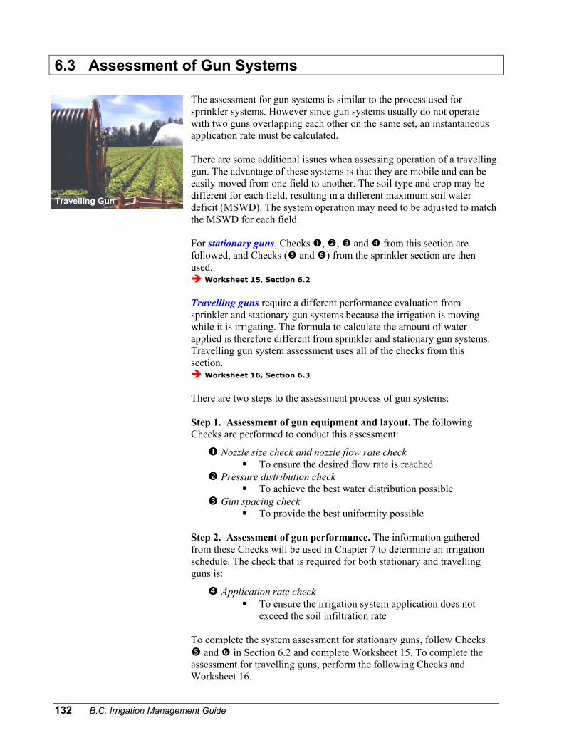
6.3 Assessment of Gun Systems The assessment for gun systems is similar to the process used for sprinkler systems. However since gun systems usually do not operate with two guns overlapping each other on the same set, an instantaneous application rate must be calculated. There are some additional issues when assessing operation of a travelling gun. The advantage of these systems is that they are mobile and can be easily moved from one field to another. The soil type and crop may be different for each field, resulting in a different maximum soil water deficit (MSWD). The system operation may need to be adjusted to match the MSWD for each field. For stationary guns, Checks , , and from this section are followed, and Checks ( and ) from the sprinkler section are then used.
Worksheet 15, Section 6.2 Travelling guns require a different performance evaluation from sprinkler and stationary gun systems because the irrigation is moving while it is irrigating. The formula to calculate the amount of water applied is therefore different from sprinkler and stationary gun systems. Travelling gun system assessment uses all of the checks from this section.
Worksheet 16, Section 6.3 There are two steps to the assessment process of gun systems: Step 1. Assessment of gun equipment and layout. The following Checks are performed to conduct this assessment:
Nozzle size check and nozzle flow rate check To ensure the desired flow rate is reached
Pressure distribution check To achieve the best water distribution possible
Gun spacing check To provide the best uniformity possible
Step 2. Assessment of gun performance. The information gathered from these Checks will be used in Chapter 7 to determine an irrigation schedule. The check that is required for both stationary and travelling guns is:
Application rate check To ensure the irrigation system application does not
exceed the soil infiltration rate To complete the system assessment for stationary guns, follow Checks
and in Section 6.2 and complete Worksheet 15. To complete the assessment for travelling guns, perform the following Checks and Worksheet 16.
Travelling Gun
Chapter 6 Irrigation System Assessment 133
Travel speed check To ensure the maximum soil water deficit (MSWD) is
not exceeded. Irrigation interval check
To ensure the next irrigation occurs in time to replenish the soil water
Step 1. Assessment of Gun System Equipment and Layout
Nozzle Size Check and Nozzle Flow Rate Check There are two types of nozzle systems for gun systems – taper bore and ring nozzles. The first step is to determine what type of nozzle is being used. Taper bore nozzles will usually have a larger wetted diameter than ring nozzles. Since the nozzles are quite large they cannot be checked for wear using a drill bit. The nozzle size is usually stamped on the nozzle and can be visually checked for wear or accurately measured using a calliper. Install a new nozzle if it appears that the nozzle is worn. Tables 4.2, 4.3 and 4.4 of the B.C. Sprinkler Irrigation Manual provide the gun flow rates based on nozzle types, size and operating pressures. Flow rates for guns can be found in the B.C. Sprinkler Irrigation Manual.
B.C. Sprinkler Irrigation Manual
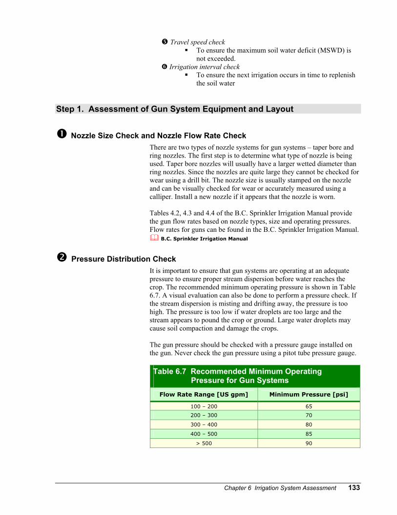
Pressure Distribution Check It is important to ensure that gun systems are operating at an adequate pressure to ensure proper stream dispersion before water reaches the crop. The recommended minimum operating pressure is shown in Table 6.7. A visual evaluation can also be done to perform a pressure check. If the stream dispersion is misting and drifting away, the pressure is too high. The pressure is too low if water droplets are too large and the stream appears to pound the crop or ground. Large water droplets may cause soil compaction and damage the crops. The gun pressure should be checked with a pressure gauge installed on the gun. Never check the gun pressure using a pitot tube pressure gauge. Table 6.7 Recommended Minimum Operating
Pressure for Gun Systems
Flow Rate Range [US gpm] Minimum Pressure [psi]
100 – 200 65
200 – 300 70
300 – 400 80
400 – 500 85
> 500 90
134 B.C. Irrigation Management Guide
Gun systems operate at very high pressures and require the installation of a pressure gauge to obtain pressure readings. Do not attempt to obtain the operating pressure with a pitot tube gauge as it is very dangerous and can cause serious injury.
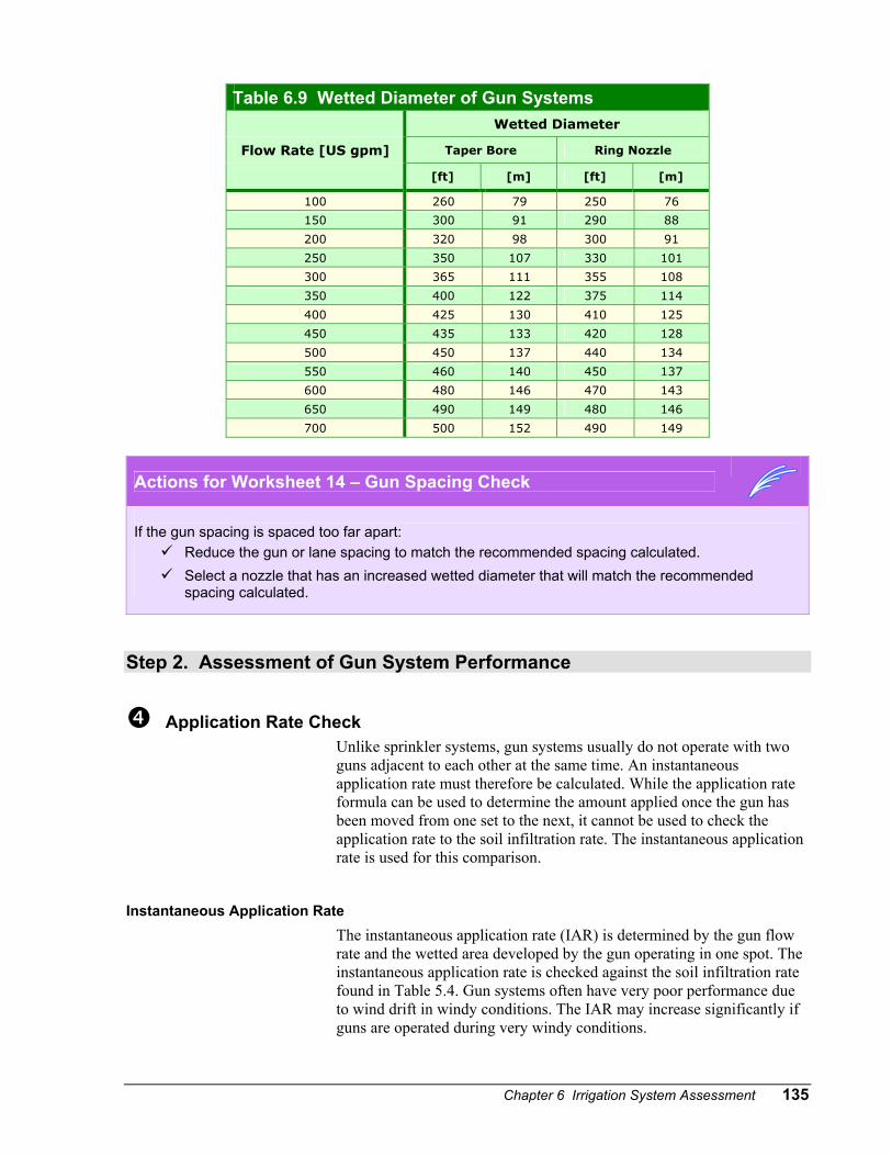
Gun Spacing Check To ensure good uniformity, the maximum gun spacing should not exceed the recommended spacing as calculated in Equation 6.9. This equation can be used to calculate the spacing of stationary guns and the lane spacing for travelling guns. Travelling guns can be spaced slightly further apart than stationary guns as the uniformity is improved by a travelling machine. Worksheet 14 can be used for stationary and travelling gun spacing assessment as well as sprinkler spacing assessment. Table 6.8 shows the recommended spacing as a percentage of the wetted diameter. Table 6.9 provides nominal information on the gun wetted diameter based on the gun flow rate and operating pressure. If available actual gun performance charts should be used as they are more accurate.
Equation 6.9 Recommended Spacing Worksheet 14
DiameterWettedofPercentageaasAllowedSpacingDiameterWettedGunSpacingecommendedR
×=
where Recommended Spacing =Gun Wetted Diameter =
Spacing Allowed as a Percentage =
appropriate spacing [ft] value from Table 6.9 [ft] value from Table 6.8 according to wind speed [%]
Table 6.8 Recommended Spacing for Gun Systems
Spacing as a Percentage of Wetted Diameter Wind Speed [km/hr]
Stationary Gun Travelling Gun
≤ 6.5 50% 60%
6.5 – 13 40% 50%
> 13 Do not operate 40%
DANGER
Chapter 6 Irrigation System Assessment 135
Table 6.9 Wetted Diameter of Gun Systems Wetted Diameter
Flow Rate [US gpm] Taper Bore Ring Nozzle
[ft] [m] [ft] [m]
100 260 79 250 76
150 300 91 290 88
200 320 98 300 91
250 350 107 330 101
300 365 111 355 108
350 400 122 375 114
400 425 130 410 125
450 435 133 420 128
500 450 137 440 134
550 460 140 450 137
600 480 146 470 143
650 490 149 480 146
700 500 152 490 149
Actions for Worksheet 14 – Gun Spacing Check
If the gun spacing is spaced too far apart:
Reduce the gun or lane spacing to match the recommended spacing calculated. Select a nozzle that has an increased wetted diameter that will match the recommended
spacing calculated.
Step 2. Assessment of Gun System Performance
Application Rate Check Unlike sprinkler systems, gun systems usually do not operate with two guns adjacent to each other at the same time. An instantaneous application rate must therefore be calculated. While the application rate formula can be used to determine the amount applied once the gun has been moved from one set to the next, it cannot be used to check the application rate to the soil infiltration rate. The instantaneous application rate is used for this comparison.
Instantaneous Application Rate The instantaneous application rate (IAR) is determined by the gun flow rate and the wetted area developed by the gun operating in one spot. The instantaneous application rate is checked against the soil infiltration rate found in Table 5.4. Gun systems often have very poor performance due to wind drift in windy conditions. The IAR may increase significantly if guns are operated during very windy conditions.
136 B.C. Irrigation Management Guide
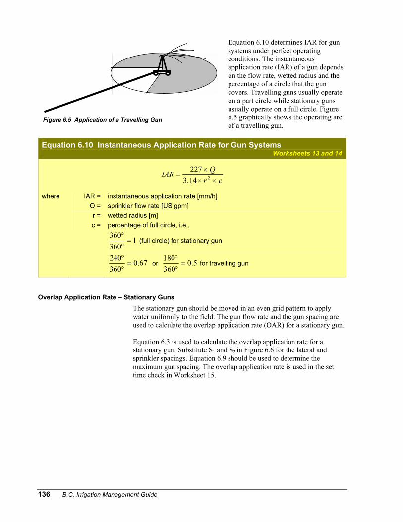
Figure 6.5 Application of a Travelling Gun
Equation 6.10 determines IAR for gun systems under perfect operating conditions. The instantaneous application rate (IAR) of a gun depends on the flow rate, wetted radius and the percentage of a circle that the gun covers. Travelling guns usually operate on a part circle while stationary guns usually operate on a full circle. Figure 6.5 graphically shows the operating arc of a travelling gun.
Equation 6.10 Instantaneous Application Rate for Gun Systems Worksheets 13 and 14
crQIAR××
×= 214.3
227
where
IAR = Q = r = c =
instantaneous application rate [mm/h] sprinkler flow rate [US gpm] wetted radius [m] percentage of full circle, i.e.,
1360360
=°°
(full circle) for stationary gun
67.0360240
=°°
or 5.0360180
=°°
for travelling gun
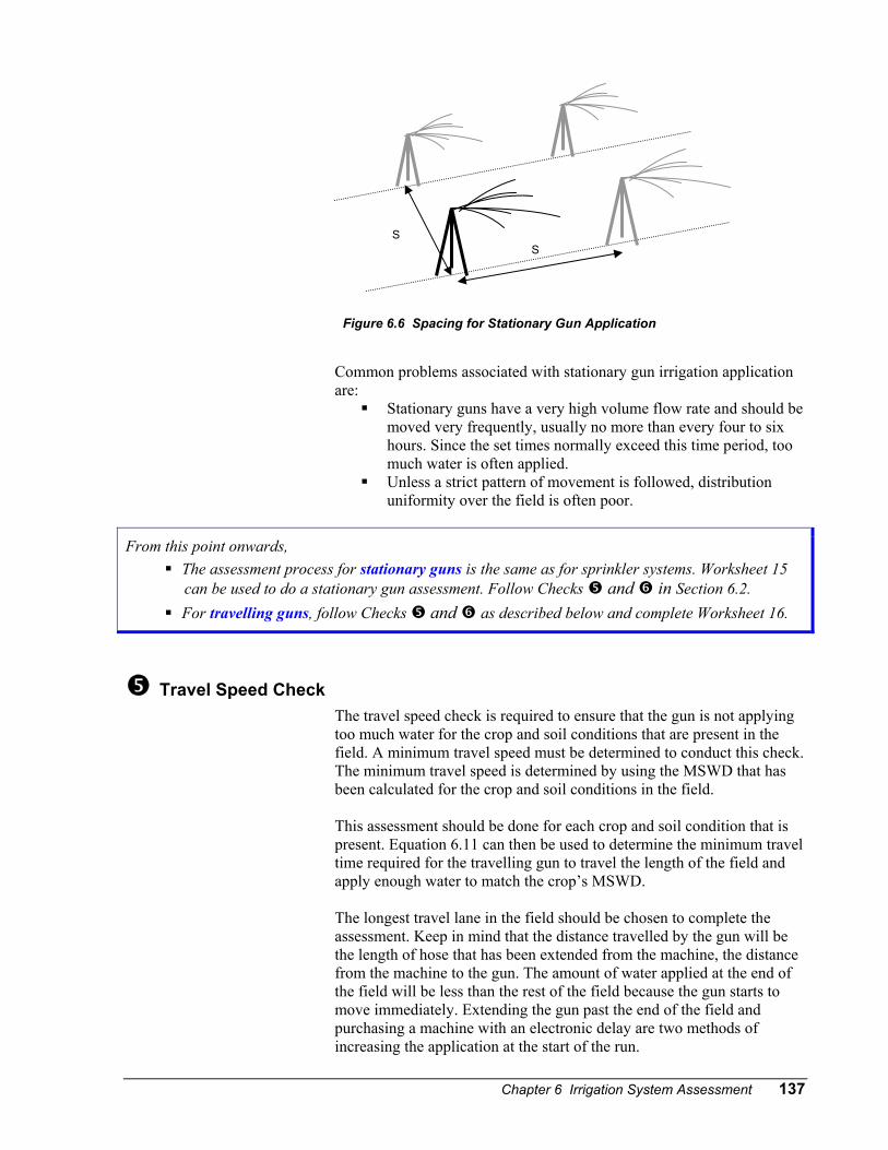
Overlap Application Rate – Stationary Guns The stationary gun should be moved in an even grid pattern to apply water uniformly to the field. The gun flow rate and the gun spacing are used to calculate the overlap application rate (OAR) for a stationary gun. Equation 6.3 is used to calculate the overlap application rate for a stationary gun. Substitute S1 and S2 in Figure 6.6 for the lateral and sprinkler spacings. Equation 6.9 should be used to determine the maximum gun spacing. The overlap application rate is used in the set time check in Worksheet 15.
Chapter 6 Irrigation System Assessment 137
Common problems associated with stationary gun irrigation application are:
Stationary guns have a very high volume flow rate and should be moved very frequently, usually no more than every four to six hours. Since the set times normally exceed this time period, too much water is often applied.
Unless a strict pattern of movement is followed, distribution uniformity over the field is often poor.
From this point onwards, The assessment process for stationary guns is the same as for sprinkler systems. Worksheet 15
can be used to do a stationary gun assessment. Follow Checks and in Section 6.2. For travelling guns, follow Checks and as described below and complete Worksheet 16.
Travel Speed Check
The travel speed check is required to ensure that the gun is not applying too much water for the crop and soil conditions that are present in the field. A minimum travel speed must be determined to conduct this check. The minimum travel speed is determined by using the MSWD that has been calculated for the crop and soil conditions in the field. This assessment should be done for each crop and soil condition that is present. Equation 6.11 can then be used to determine the minimum travel time required for the travelling gun to travel the length of the field and apply enough water to match the crop’s MSWD. The longest travel lane in the field should be chosen to complete the assessment. Keep in mind that the distance travelled by the gun will be the length of hose that has been extended from the machine, the distance from the machine to the gun. The amount of water applied at the end of the field will be less than the rest of the field because the gun starts to move immediately. Extending the gun past the end of the field and purchasing a machine with an electronic delay are two methods of increasing the application at the start of the run.
SS
Figure 6.6 Spacing for Stationary Gun Application
138 B.C. Irrigation Management Guide
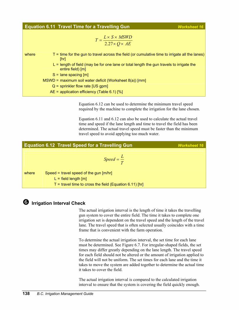
Equation 6.11 Travel Time for a Travelling Gun Worksheet 16
AEQMSWDSLT××
××=
27.2
where
T =
L =
S = MSWD =
Q = AE =
time for the gun to travel across the field (or cumulative time to irrigate all the lanes) [hr] length of field (may be for one lane or total length the gun travels to irrigate the entire field) [m] lane spacing [m] maximum soil water deficit (Worksheet 8(a)) [mm] sprinkler flow rate [US gpm] application efficiency (Table 6.1) [%]
Equation 6.12 can be used to determine the minimum travel speed required by the machine to complete the irrigation for the lane chosen. Equation 6.11 and 6.12 can also be used to calculate the actual travel time and speed if the lane length and time to travel the field has been determined. The actual travel speed must be faster than the minimum travel speed to avoid applying too much water.
Equation 6.12 Travel Speed for a Travelling Gun Worksheet 16
TLSpeed =
where
Speed = L = T =
travel speed of the gun [m/hr] field length [m] travel time to cross the field (Equation 6.11) [hr]
Irrigation Interval Check
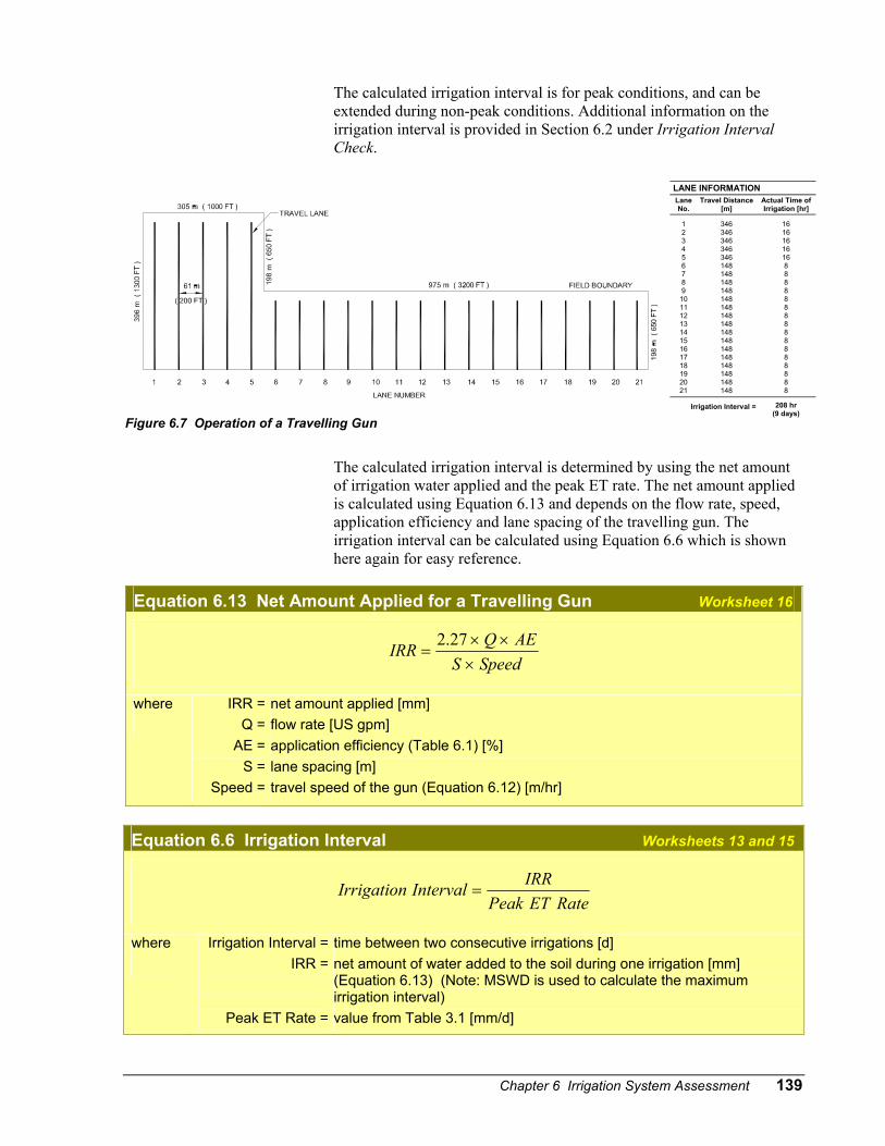
The actual irrigation interval is the length of time it takes the travelling gun system to cover the entire field. The time it takes to complete one irrigation set is dependent on the travel speed and the length of the travel lane. The travel speed that is often selected usually coincides with a time frame that is convenient with the farm operation. To determine the actual irrigation interval, the set time for each lane must be determined. See Figure 6.7. For irregular-shaped fields, the set times may differ greatly depending on the lane length. The travel speed for each field should not be altered or the amount of irrigation applied to the field will not be uniform. The set times for each lane and the time it takes to move the system are added together to determine the actual time it takes to cover the field. The actual irrigation interval is compared to the calculated irrigation interval to ensure that the system is covering the field quickly enough.
Chapter 6 Irrigation System
L
The calculated irrigation interval is for peak conditions, and can be extended during non-peak conditions. Additional information on the irrigation interval is provided in Section 6.2 under Irrigation Interval Check.
Figure 6.7 Operation of a Travelling Gun
The calculated irrigation interval is determined by usiof irrigation water applied and the peak ET rate. The nis calculated using Equation 6.13 and depends on the application efficiency and lane spacing of the travellinirrigation interval can be calculated using Equation 6.here again for easy reference.
Equation 6.13 Net Amount Applied for a Travelling Gun
SpeedSAEQIRR
×××
=27.2
where
IRR =Q =
AE =S =
Speed =
net amount applied [mm] flow rate [US gpm] application efficiency (Table 6.1) [%] lane spacing [m] travel speed of the gun (Equation 6.12) [m/hr]
Equation 6.6 Irrigation Interval Work
RateETPeakIRRIntervalIrrigation =
where
Irrigation Interval = IRR =
Peak ET Rate =
time between two consecutive irrigations [d] net amount of water added to the soil during one irriga(Equation 6.13) (Note: MSWD is used to calculate theirrigation interval) value from Table 3.1 [mm/d]
ANE INFORMATION Lane No.
Travel Distance [m]
Actual Time of Irrigation [hr]
1 2 3 4 5 6 7 8 9 10 11 12 13 14 15 16 17 18 19 20 21
346 346 346 346 346 148 148 148 148 148 148 148 148 148 148 148 148 148 148 148 148
16 16 16 16 16 8 8 8 8 8 8 8 8 8 8 8 8 8 8 8 8
Assessment 139
Irrigation Interval = 208 hr (9 days)
ng the net amount et amount applied
flow rate, speed, g gun. The
6 which is shown
Worksheet 16
sheets 13 and 15
tion [mm] maximum
140 B.C. Irrigation Management Guide
Table 5.2 in the B.C. Sprinkler Irrigation Manual can be used to determine the amount of water applied by travelling guns for various flow rates and travel speeds.
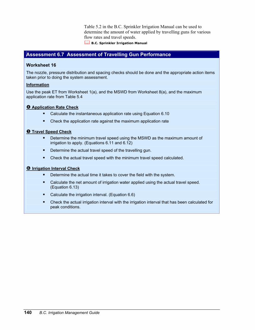
B.C. Sprinkler Irrigation Manual Assessment 6.7 Assessment of Travelling Gun Performance Worksheet 16 The nozzle, pressure distribution and spacing checks should be done and the appropriate action items taken prior to doing the system assessment.
Information
Use the peak ET from Worksheet 1(a), and the MSWD from Worksheet 8(a), and the maximum application rate from Table 5.4
Application Rate Check
Calculate the instantaneous application rate using Equation 6.10
Check the application rate against the maximum application rate
Travel Speed Check Determine the minimum travel speed using the MSWD as the maximum amount of
irrigation to apply. (Equations 6.11 and 6.12)
Determine the actual travel speed of the travelling gun.
Check the actual travel speed with the minimum travel speed calculated.
Irrigation Interval Check Determine the actual time it takes to cover the field with the system.
Calculate the net amount of irrigation water applied using the actual travel speed. (Equation 6.13)
Calculate the irrigation interval. (Equation 6.6)
Check the actual irrigation interval with the irrigation interval that has been calculated for peak conditions.
Chapter 6 Irrigation System Assessment 141
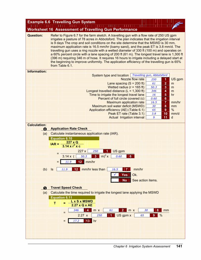
Example 6.6 Travelling Gun System
Worksheet 16 Assessment of Travelling Gun Performance
Question:
Refer to Figure 6.7 for the farm sketch. A travelling gun with a flow rate of 250 US gpm irrigates a pasture of 78 acres in Abbotsford. The plan indicates that the irrigation interval is 9 days The crop and soil conditions on the site determine that the MSWD is 30 mm, maximum application rate is 16.5 mm/hr (loamy sand), and the peak ET is 3.8 mm/d. The travelling gun uses a ring nozzle with a wetted diameter of 330 ft (100 m) and operates on a 60% percent circle with a lane spacing of 200 ft (61 m). The longest travel lane is 1,300 ft (396 m) requiring 346 m of hose. It requires 16 hours to irrigate including a delayed start at the beginning to improve uniformity. The application efficiency of the travelling gun is 65% from Table 6.1.
Information: System type and location Travelling gun, Abbotsford
Nozzle flow rate 250 1 US gpm Lane spacing (S = 200 ft) 61 2 m Wetted radius (r = 165 ft) 50.3 3 m Longest travelled distance (L = 1,300 ft) 346 4 m Time to irrigate the longest travel lane 16 5 hr Percent of full circle covered (c) 0.60 6 Maximum application rate 16.5 7 mm/hr Maximum soil water deficit (MSWD) 30 8 mm Application efficiency (AE) (Table 6.1) 65 9 % Peak ET rate (Table 3.1) 3.8 10 mm/d Actual Irrigation interval 9 11 d Calculation: Application Rate Check (a) Calculate instantaneous application rate (IAR). Equation 6.10 227 x Q IAR = 3.14 x r2 x c 227 x 250 1 US gpm
= 3.14 x ( 50.3 3 m)2 x 0.60 6
= 11.9 12 mm/hr (b) Is 11.9 12 mm/hr less than 16.5 7 mm/hr
Yes Ok. No See action items. Travel Speed Check (a) Calculate the time required to irrigate the longest lane applying the MSWD Equation 6.11 L x S x MSWD T = 2.27 x Q x AE 346 4 m x 61 2 m x 30 8 mm
= 2.27 x 250 1 US gpm x 65 9 %
= 17.2 13 hr
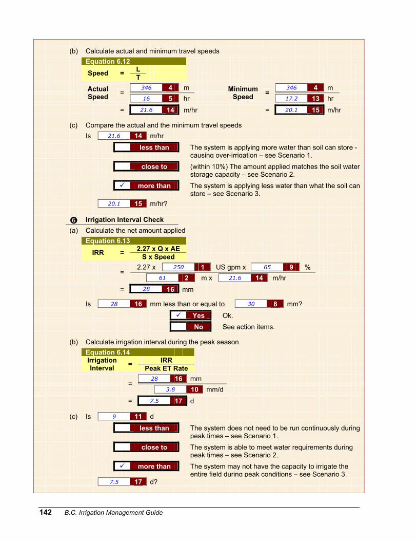
142 B.C. Irrigation Management Guide
(b) Calculate actual and minimum travel speeds Equation 6.12 L Speed = T 346 4 m 346 4 m
Actual Speed =
16 5 hrMinimum
Speed = 17.2 13 hr
= 21.6 14 m/hr = 20.1 15 m/hr (c) Compare the actual and the minimum travel speeds Is 21.6 14 m/hr
less than
The system is applying more water than soil can store - causing over-irrigation – see Scenario 1.
close to
(within 10%) The amount applied matches the soil water storage capacity – see Scenario 2.
more than
The system is applying less water than what the soil can store – see Scenario 3.
20.1 15 m/hr? Irrigation Interval Check
(a) Calculate the net amount applied Equation 6.13 2.27 x Q x AE IRR = S x Speed 2.27 x 250 1 US gpm x 65 9 %
= 61 2 m x 21.6 14 m/hr
= 28 16 mm Is 28 16 mm less than or equal to 30 8 mm?
Yes Ok. No See action items. (b) Calculate irrigation interval during the peak season Equation 6.14 IRR
Irrigation Interval = Peak ET Rate
28 16 mm
= 3.8 10 mm/d
= 7.5 17 d (c) Is 9 11 d
less than
The system does not need to be run continuously during peak times – see Scenario 1.
close to
The system is able to meet water requirements during peak times – see Scenario 2.
more than
The system may not have the capacity to irrigate the entire field during peak conditions – see Scenario 3.
7.5 17 d?
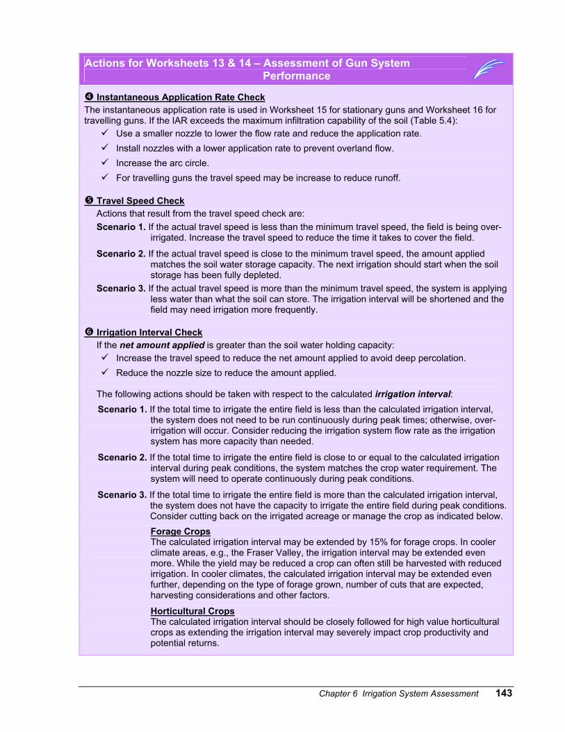
Chapter 6 Irrigation System Assessment 143
Actions for Worksheets 13 & 14 – Assessment of Gun System Performance
Instantaneous Application Rate Check The instantaneous application rate is used in Worksheet 15 for stationary guns and Worksheet 16 for travelling guns. If the IAR exceeds the maximum infiltration capability of the soil (Table 5.4):
Use a smaller nozzle to lower the flow rate and reduce the application rate. Install nozzles with a lower application rate to prevent overland flow. Increase the arc circle. For travelling guns the travel speed may be increase to reduce runoff.
Travel Speed Check Actions that result from the travel speed check are: Scenario 1. If the actual travel speed is less than the minimum travel speed, the field is being over-
irrigated. Increase the travel speed to reduce the time it takes to cover the field.
Scenario 2. If the actual travel speed is close to the minimum travel speed, the amount applied matches the soil water storage capacity. The next irrigation should start when the soil storage has been fully depleted.
Scenario 3. If the actual travel speed is more than the minimum travel speed, the system is applying less water than what the soil can store. The irrigation interval will be shortened and the field may need irrigation more frequently.
Irrigation Interval Check If the net amount applied is greater than the soil water holding capacity:
Increase the travel speed to reduce the net amount applied to avoid deep percolation. Reduce the nozzle size to reduce the amount applied.
The following actions should be taken with respect to the calculated irrigation interval: Scenario 1. If the total time to irrigate the entire field is less than the calculated irrigation interval,
the system does not need to be run continuously during peak times; otherwise, over-irrigation will occur. Consider reducing the irrigation system flow rate as the irrigation system has more capacity than needed.
Scenario 2. If the total time to irrigate the entire field is close to or equal to the calculated irrigation interval during peak conditions, the system matches the crop water requirement. The system will need to operate continuously during peak conditions.
Scenario 3. If the total time to irrigate the entire field is more than the calculated irrigation interval, the system does not have the capacity to irrigate the entire field during peak conditions. Consider cutting back on the irrigated acreage or manage the crop as indicated below. Forage Crops The calculated irrigation interval may be extended by 15% for forage crops. In cooler climate areas, e.g., the Fraser Valley, the irrigation interval may be extended even more. While the yield may be reduced a crop can often still be harvested with reduced irrigation. In cooler climates, the calculated irrigation interval may be extended even further, depending on the type of forage grown, number of cuts that are expected, harvesting considerations and other factors.
Horticultural Crops The calculated irrigation interval should be closely followed for high value horticultural crops as extending the irrigation interval may severely impact crop productivity and potential returns.
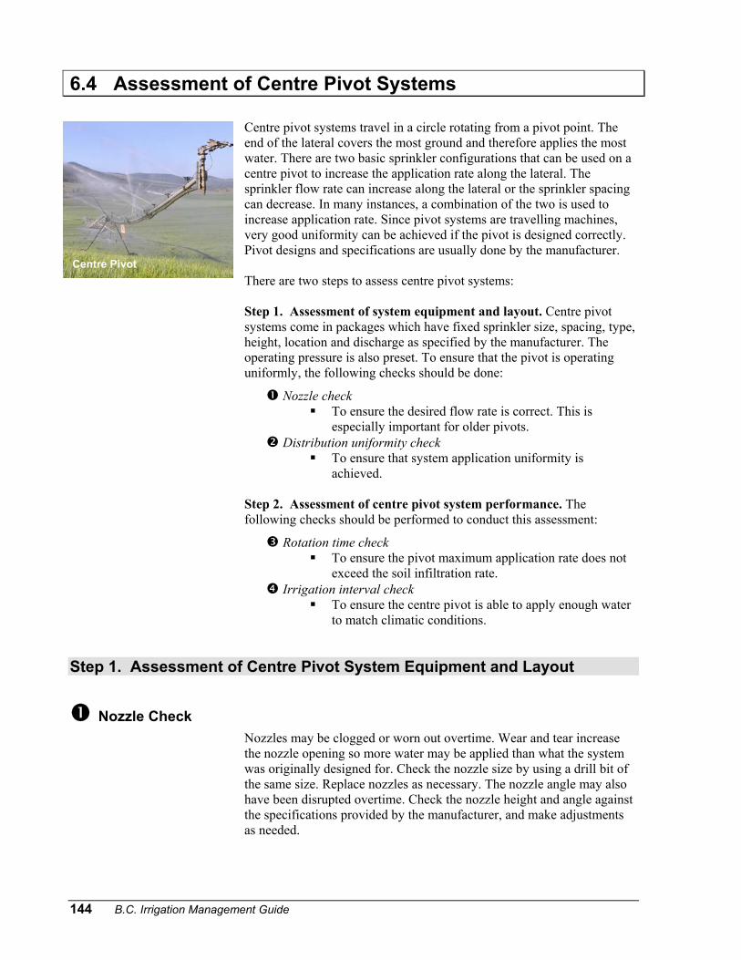
144 B.C. Irrigation Management Guide
6.4 Assessment of Centre Pivot Systems Centre pivot systems travel in a circle rotating from a pivot point. The end of the lateral covers the most ground and therefore applies the most water. There are two basic sprinkler configurations that can be used on a centre pivot to increase the application rate along the lateral. The sprinkler flow rate can increase along the lateral or the sprinkler spacing can decrease. In many instances, a combination of the two is used to increase application rate. Since pivot systems are travelling machines, very good uniformity can be achieved if the pivot is designed correctly. Pivot designs and specifications are usually done by the manufacturer. There are two steps to assess centre pivot systems: Step 1. Assessment of system equipment and layout. Centre pivot systems come in packages which have fixed sprinkler size, spacing, type, height, location and discharge as specified by the manufacturer. The operating pressure is also preset. To ensure that the pivot is operating uniformly, the following checks should be done:
Nozzle check To ensure the desired flow rate is correct. This is
especially important for older pivots. Distribution uniformity check
To ensure that system application uniformity is achieved.
Step 2. Assessment of centre pivot system performance. The following checks should be performed to conduct this assessment:
Rotation time check To ensure the pivot maximum application rate does not
exceed the soil infiltration rate. Irrigation interval check
To ensure the centre pivot is able to apply enough water to match climatic conditions.
Step 1. Assessment of Centre Pivot System Equipment and Layout
Nozzle Check Nozzles may be clogged or worn out overtime. Wear and tear increase the nozzle opening so more water may be applied than what the system was originally designed for. Check the nozzle size by using a drill bit of the same size. Replace nozzles as necessary. The nozzle angle may also have been disrupted overtime. Check the nozzle height and angle against the specifications provided by the manufacturer, and make adjustments as needed.
Centre Pivot
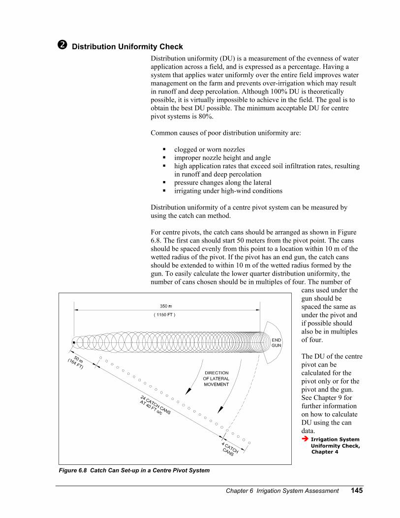
Chapter 6 Irrigation System Assessment 145
Figure 6.8 Catch Can Set-up in a Centre Pivot System
Distribution Uniformity Check Distribution uniformity (DU) is a measurement of the evenness of water application across a field, and is expressed as a percentage. Having a system that applies water uniformly over the entire field improves water management on the farm and prevents over-irrigation which may result in runoff and deep percolation. Although 100% DU is theoretically possible, it is virtually impossible to achieve in the field. The goal is to obtain the best DU possible. The minimum acceptable DU for centre pivot systems is 80%. Common causes of poor distribution uniformity are:
clogged or worn nozzles improper nozzle height and angle high application rates that exceed soil infiltration rates, resulting
in runoff and deep percolation pressure changes along the lateral irrigating under high-wind conditions
Distribution uniformity of a centre pivot system can be measured by using the catch can method. For centre pivots, the catch cans should be arranged as shown in Figure 6.8. The first can should start 50 meters from the pivot point. The cans should be spaced evenly from this point to a location within 10 m of the wetted radius of the pivot. If the pivot has an end gun, the catch cans should be extended to within 10 m of the wetted radius formed by the gun. To easily calculate the lower quarter distribution uniformity, the number of cans chosen should be in multiples of four. The number of
cans used under the gun should be spaced the same as under the pivot and if possible should also be in multiples of four. The DU of the centre pivot can be calculated for the pivot only or for the pivot and the gun. See Chapter 9 for further information on how to calculate DU using the can data.
Irrigation System Uniformity Check, Chapter 4
146 B.C. Irrigation Management Guide
Step 2. Assessment of Centre Pivot System Performance
Rotation Time Check
Centre pivot systems can cover a field quite quickly. At top speed, the amount of water applied to the crop will be much less than what can be stored in the soil, i.e., MSWD. The limiting factor for centre pivots is usually the application rate, especially for larger pivots. The last tower of the pivot travels much more quickly than the towers closer to the pivot point. The amount of water applied by the system must be uniform over the entire field; therefore, the application rate increases proportionally as the sprinklers go farther from the pivot point. The maximum application rate of a centre pivot system occurs at the end of the lateral where most of the water is applied. To reduce puddling and runoff, the maximum application rate should not exceed the maximum soil infiltration rate. While the application rate is higher, the time of application is also much shorter. Maximum soil infiltration rates are also much higher for short durations than they are for longer irrigation set times. As the irrigation time increases, the soil water tension decreases; thus, the infiltration rate drops. Figures 6.9(a) and 6.9(b) provide general guidance on the maximum infiltration rates of several common soil types for durations less than an hour. These charts can be used as a guide to estimate the maximum duration of application (Tm) for center pivots as used in Equation 6.15. The maximum pivot application rate (PAR) is calculated for the end tower. The PAR depends on the pivot flow rate (Q), effective wetted radius of the pivot (R) and wetted radius (r) of the large sprinkler near the end of the pivot. Note that sprinklers with a small effective wetted radius (r) will have shorter application durations, requiring a higher application rate to apply the same amount of water as sprinklers with a larger wetted radius. The wetted radius of the pivot and the end sprinklers can be measured or obtained from manufacturer’s charts. To estimate PAR, the pivot flow rate must also be known. This information is also obtained from the manufacturer. Information on determining flow rate requirements for new pivots can be obtained from the B.C. Sprinkler Irrigation Manual.
B.C. Sprinkler Irrigation Manual
The PAR is calculated using Equation 6.14. The PAR calculated should match the maximum soil infiltration rate if runoff is to be prevented. The value calculated for the PAR should be used as the infiltration rate value in Figure 6.9. Using the PAR infiltration rate value, the maximum duration of application (Tm) can then be determined using Figure 6.9. The centre pivot minimum travel speed can then be calculated using Equation 6.15 using the Tm value obtained from Figure 6.9.
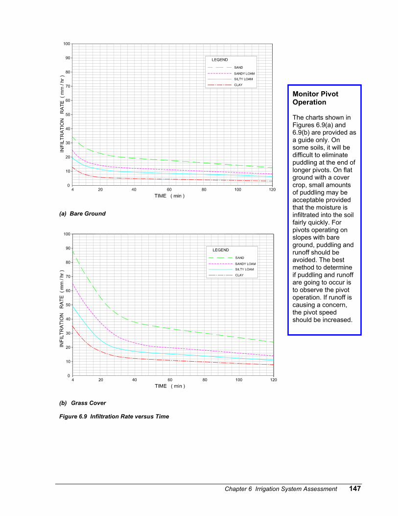
(b) G Figu
(a) Bare Ground
rass Cover
re 6.9 Infiltration Rate versus Time
Chapter 6 Irrigation Sys
Monitor Pivot Operation The charts shown in Figures 6.9(a) and 6.9(b) are provided asa guide only. On some soils, it will be difficult to eliminate puddling at the end of longer pivots. On flat ground with a cover crop, small amounts of puddling may be acceptable provided that the moisture is infiltrated into the soil fairly quickly. For pivots operating on slopes with bare ground, puddling and runoff should be avoided. The best method to determine if puddling and runoff are going to occur is to observe the pivot operation. If runoff is causing a concern, the pivot speed should be increased.
tem Assessment 147
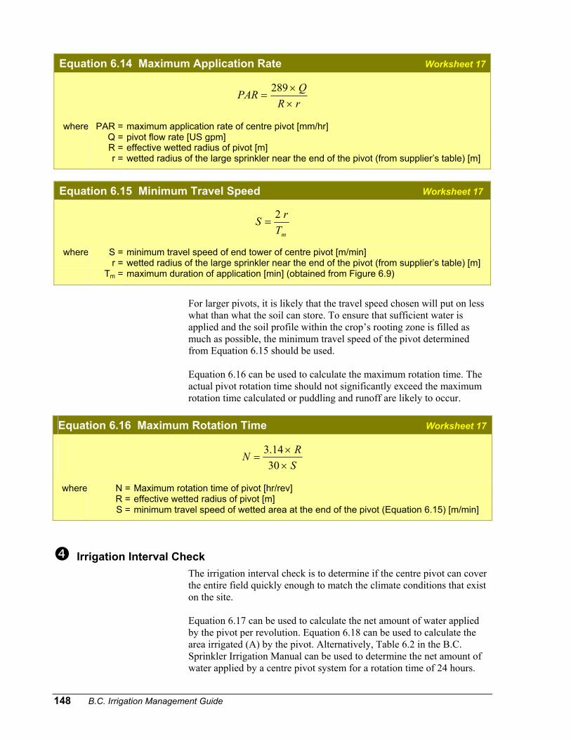
148 B.C. Irrigation Management Guide
Equation 6.14 Maximum Application Rate Worksheet 17
rRQPAR
××
=289
where PAR = maximum application rate of centre pivot [mm/hr] Q = pivot flow rate [US gpm] R = effective wetted radius of pivot [m] r = wetted radius of the large sprinkler near the end of the pivot (from supplier’s table) [m]
Equation 6.15 Minimum Travel Speed Worksheet 17
mTrS 2
=
where S = minimum travel speed of end tower of centre pivot [m/min] r = wetted radius of the large sprinkler near the end of the pivot (from supplier’s table) [m] Tm = maximum duration of application [min] (obtained from Figure 6.9)
For larger pivots, it is likely that the travel speed chosen will put on less what than what the soil can store. To ensure that sufficient water is applied and the soil profile within the crop’s rooting zone is filled as much as possible, the minimum travel speed of the pivot determined from Equation 6.15 should be used. Equation 6.16 can be used to calculate the maximum rotation time. The actual pivot rotation time should not significantly exceed the maximum rotation time calculated or puddling and runoff are likely to occur.
Equation 6.16 Maximum Rotation Time Worksheet 17
SRN
××
=3014.3
where N = Maximum rotation time of pivot [hr/rev] R = effective wetted radius of pivot [m] S = minimum travel speed of wetted area at the end of the pivot (Equation 6.15) [m/min]
Irrigation Interval Check
The irrigation interval check is to determine if the centre pivot can cover the entire field quickly enough to match the climate conditions that exist on the site. Equation 6.17 can be used to calculate the net amount of water applied by the pivot per revolution. Equation 6.18 can be used to calculate the area irrigated (A) by the pivot. Alternatively, Table 6.2 in the B.C. Sprinkler Irrigation Manual can be used to determine the net amount of water applied by a centre pivot system for a rotation time of 24 hours.
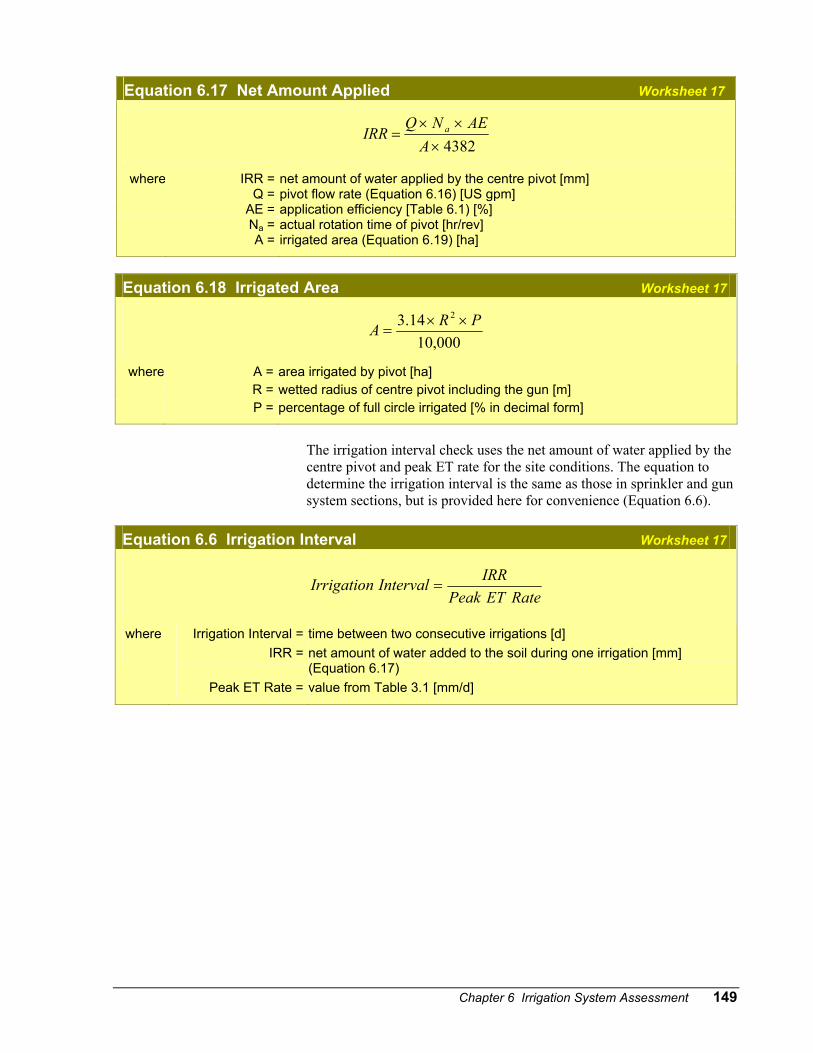
Chapter 6 Irrigation System Assessment 149
Equation 6.17 Net Amount Applied Worksheet 17
4382×××
=A
AENQIRR a
where IRR = net amount of water applied by the centre pivot [mm] Q = pivot flow rate (Equation 6.16) [US gpm] AE = application efficiency [Table 6.1) [%] Na = actual rotation time of pivot [hr/rev] A = irrigated area (Equation 6.19) [ha]
Equation 6.18 Irrigated Area Worksheet 17
000,1014.3 2 PRA ××
=
where A = area irrigated by pivot [ha] R = wetted radius of centre pivot including the gun [m] P = percentage of full circle irrigated [% in decimal form]
The irrigation interval check uses the net amount of water applied by the centre pivot and peak ET rate for the site conditions. The equation to determine the irrigation interval is the same as those in sprinkler and gun system sections, but is provided here for convenience (Equation 6.6).
Equation 6.6 Irrigation Interval Worksheet 17
RateETPeakIRRIntervalIrrigation =
where
Irrigation Interval = IRR =
Peak ET Rate =
time between two consecutive irrigations [d] net amount of water added to the soil during one irrigation [mm] (Equation 6.17) value from Table 3.1 [mm/d]
150 B.C. Irrigation Management Guide
Assessment 6.8 Assessment of Centre Pivot Performance
Worksheet 17
The nozzle and distribution uniformity checks should be done prior to performing the system assessment.
Rotation Time Check
Calculate the pivot maximum application rate
Calculate the minimum travel speed
Calculate the maximum rotation time, and compare it with the actual time
Irrigation Interval Check
Calculate the area irrigated by the pivot
Calculate the net amount applied, and compare it with the MSWD
Calculate the irrigation interval, and compare it with the actual value
Note: This assessment is only a guide. For more accurate results, field observation and measurements are recommended.
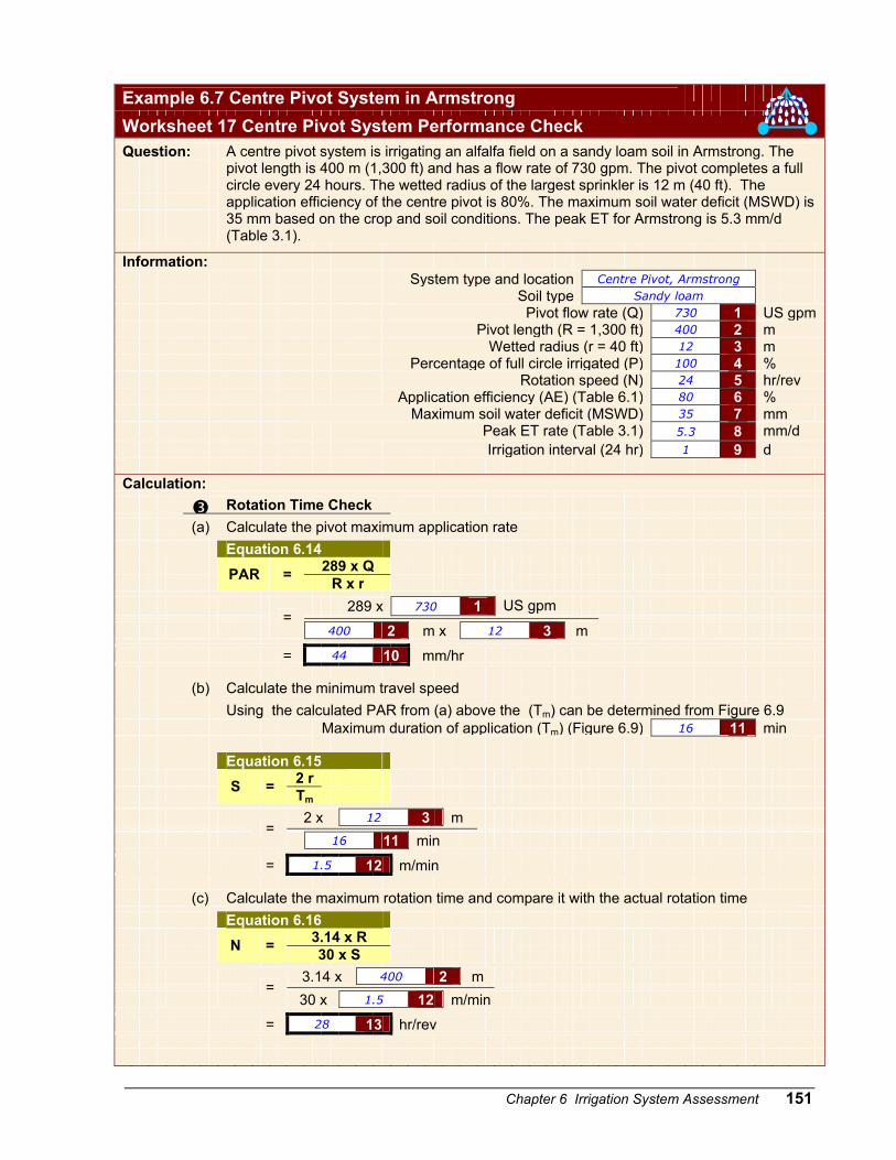
Chapter 6 Irrigation System Assessment 151
Example 6.7 Centre Pivot System in Armstrong
Worksheet 17 Centre Pivot System Performance Check Question:
A centre pivot system is irrigating an alfalfa field on a sandy loam soil in Armstrong. The pivot length is 400 m (1,300 ft) and has a flow rate of 730 gpm. The pivot completes a full circle every 24 hours. The wetted radius of the largest sprinkler is 12 m (40 ft). The application efficiency of the centre pivot is 80%. The maximum soil water deficit (MSWD) is 35 mm based on the crop and soil conditions. The peak ET for Armstrong is 5.3 mm/d (Table 3.1).
Information: System type and location Centre Pivot, Armstrong
Soil type Sandy loam
Pivot flow rate (Q) 730 1 US gpm Pivot length (R = 1,300 ft) 400 2 m Wetted radius (r = 40 ft) 12 3 m Percentage of full circle irrigated (P) 100 4 % Rotation speed (N) 24 5 hr/rev Application efficiency (AE) (Table 6.1) 80 6 % Maximum soil water deficit (MSWD) 35 7 mm Peak ET rate (Table 3.1) 5.3 8 mm/d Irrigation interval (24 hr) 1 9 d Calculation: Rotation Time Check (a) Calculate the pivot maximum application rate Equation 6.14 289 x Q PAR = R x r 289 x 730 1 US gpm
=
400 2 m x 12 3 m
= 44 10 mm/hr (b) Calculate the minimum travel speed Using the calculated PAR from (a) above the (Tm) can be determined from Figure 6.9 Maximum duration of application (Tm) (Figure 6.9) 16 11 min Equation 6.15 2 r S = Tm 2 x 12 3 m
= 16 11 min
= 1.5 12 m/min (c) Calculate the maximum rotation time and compare it with the actual rotation time Equation 6.16 3.14 x R N = 30 x S 3.14 x 400 2 m
= 30 x 1.5 12 m/min
= 28 13 hr/rev
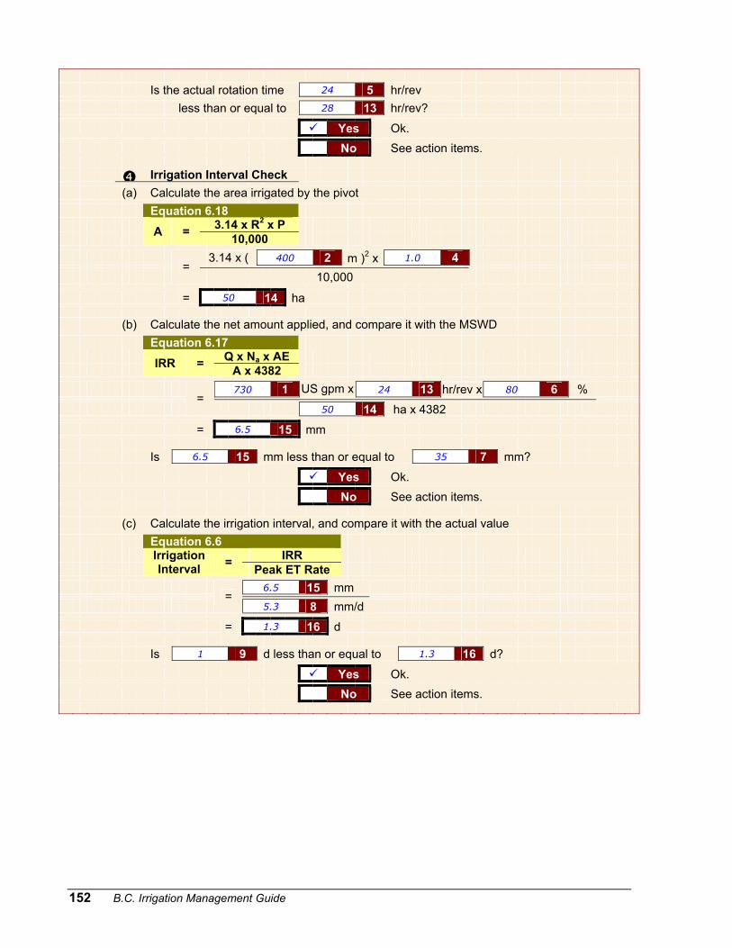
152 B.C. Irrigation Management Guide
Is the actual rotation time 24 5 hr/rev less than or equal to 28 13 hr/rev?
Yes Ok. No See action items. Irrigation Interval Check (a) Calculate the area irrigated by the pivot Equation 6.18 3.14 x R2 x P A = 10,000 3.14 x ( 400 2 m )2 x 1.0 4
=
10,000
= 50 14 ha (b) Calculate the net amount applied, and compare it with the MSWD Equation 6.17 Q x Na x AE IRR = A x 4382 730 1 US gpm x 24 13 hr/rev x 80 6 %
=
50 14 ha x 4382
= 6.5 15 mm Is 6.5 15 mm less than or equal to 35 7 mm?
Yes Ok. No See action items. (c) Calculate the irrigation interval, and compare it with the actual value Equation 6.6 IRR
Irrigation Interval = Peak ET Rate
6.5 15 mm
= 5.3 8 mm/d
= 1.3 16 d Is 1 9 d less than or equal to 1.3 16 d?
Yes Ok. No See action items.
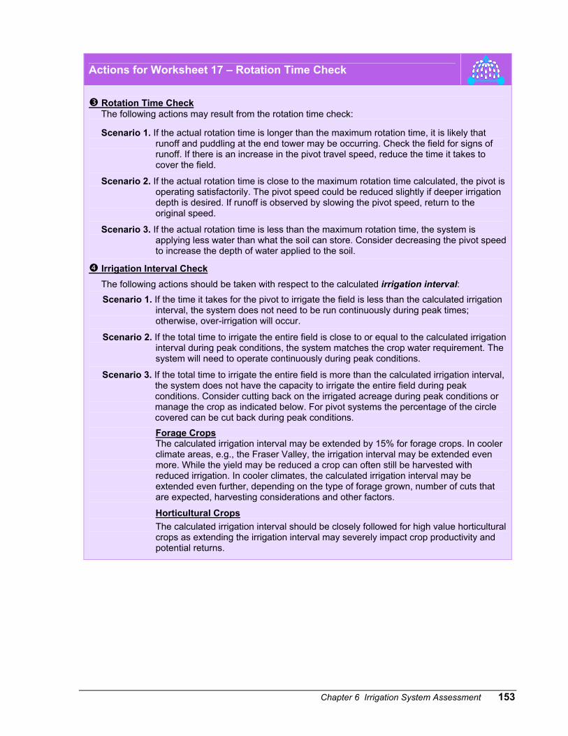
Chapter 6 Irrigation System Assessment 153
Actions for Worksheet 17 – Rotation Time Check
Rotation Time Check The following actions may result from the rotation time check:
Scenario 1. If the actual rotation time is longer than the maximum rotation time, it is likely that runoff and puddling at the end tower may be occurring. Check the field for signs of runoff. If there is an increase in the pivot travel speed, reduce the time it takes to cover the field.
Scenario 2. If the actual rotation time is close to the maximum rotation time calculated, the pivot is operating satisfactorily. The pivot speed could be reduced slightly if deeper irrigation depth is desired. If runoff is observed by slowing the pivot speed, return to the original speed.
Scenario 3. If the actual rotation time is less than the maximum rotation time, the system is applying less water than what the soil can store. Consider decreasing the pivot speed to increase the depth of water applied to the soil.
Irrigation Interval Check The following actions should be taken with respect to the calculated irrigation interval: Scenario 1. If the time it takes for the pivot to irrigate the field is less than the calculated irrigation
interval, the system does not need to be run continuously during peak times; otherwise, over-irrigation will occur.
Scenario 2. If the total time to irrigate the entire field is close to or equal to the calculated irrigation interval during peak conditions, the system matches the crop water requirement. The system will need to operate continuously during peak conditions.
Scenario 3. If the total time to irrigate the entire field is more than the calculated irrigation interval, the system does not have the capacity to irrigate the entire field during peak conditions. Consider cutting back on the irrigated acreage during peak conditions or manage the crop as indicated below. For pivot systems the percentage of the circle covered can be cut back during peak conditions. Forage Crops The calculated irrigation interval may be extended by 15% for forage crops. In cooler climate areas, e.g., the Fraser Valley, the irrigation interval may be extended even more. While the yield may be reduced a crop can often still be harvested with reduced irrigation. In cooler climates, the calculated irrigation interval may be extended even further, depending on the type of forage grown, number of cuts that are expected, harvesting considerations and other factors.
Horticultural Crops The calculated irrigation interval should be closely followed for high value horticultural crops as extending the irrigation interval may severely impact crop productivity and potential returns.
154 B.C. Irrigation Management Guide
6.5 Assessment of Trickle/Drip Systems
Drip irrigation systems usually apply small amounts of water to the crop on a very frequent basis. Drip systems operate differently than sprinkler systems as the application rates are quite low and the irrigation interval is very short. The type of product used in drip/ trickle systems is quite different from those used in sprinkler systems; therefore, requires a different assessment procedure. There are two steps to assess drip irrigation systems: Step 1. Assessment of trickle/drip equipment and layout. There are many different types of drip/trickle irrigation products that deliver water to the plant. To ensure that the drip irrigation system is operating uniformly, the following checks should be performed:
Emitter flow rate check To ensure that the emitters are delivering the amount of
water as per the system design. The emitter flow rate usually decreases over time; therefore, a flow rate check should be performed every few years.
Emitter spacing check
To ensure that the amount of water applied to each plant is uniform and that a sufficient portion of the plant’s root zone obtains water.
Pressure distribution check
This check is optional and only needs to be done if the emitter flow rate check indicates that there is a problem with uniformity. To ensure that all emitters are operating at the same pressure throughout the system.
Step 2. Assessment of trickle/drip system operating time. The information that is gathered from this check will be used to in Chapter 7 to develop an irrigation schedule.
System operating time check To determine if the amount of water applied by the
system matches the crop water requirement during peak conditions.
B.C. Trickle Irrigation Manual
Step 1. Assessment of Trickle/Drip System Equipment and Layout
Emitter Flow Rate Check
Fields irrigated with trickle systems usually have more than one zone. Each zone can be operated independently from the other zones. Each zone should contain the same type of emitters, same crop at the same
Drip
Chapter 6 Irrigation System Assessment 155
maturity, and the same soil type. If the zones have different parameters, they will need to be managed differently to optimize energy and water use. The emitter flow rate check should be done each year as the emitter flow rate decreases over time. The emitter flow rate may also decrease over the irrigation season so it is a good idea to conduct the flow rate check at the beginning of the irrigation season as well as 2/3rd of the way into the irrigation season. Worksheet 18 can be used to summarize the emitter flow rate determined for each zone. A flow meter should be installed at the filtration unit so that the flow rate for each zone can be monitored over the season. The emitter flow rate check will help determine where the flow rate decreases are occurring.
Flow Rate Measurement of Drip Line and Point Source To determine the flow rate from a drip line, a section of the drip line should be used. The flow from this section should be collected into a trough as shown in Figure 6.10(a). The procedure in Assessment 6.9 should be used to determine the flow. Emitter flow rate can be determined by measuring the amount of water collected over a given time period as shown in Figure 6.10(b). The amount of water collected should be measured using a graduated cylinder as shown in Figure 6.10(c). Take an average of at least three readings from three different emitters in that location to determine the flow rate that will be recorded. The measured flow rate can be compared to the manufacturer’s stated flow rate for that emitter. If the measured flow rate is 15% or more below the manufacturer’s values, the emitters may be clogged. Equation 6.19 can be used to calculate the flow rate for drip line and/or emitter.
Equation 6.19 Flow Rate of Emitter and Drip Line Worksheet 18
(a) Drip Line Flow Rate for 100 m of Tape
67.16520
××××
=TroughinEmittersofNumberTimeCollection
mperEmittersofNumberVolumeMeasuredRateFlowEmitter
(b) Emitter Flow Rate
67.16×=
TimeCollectionVolumeMeasuredRateFlowEmitter
where
Emitter Flow Rate = Measured Volume =
Collection Time =
spray or point source [L/hr], and drip [L/hr/100 m] total volume collected during the recommended time period [ml] time to collect measure volume [min]
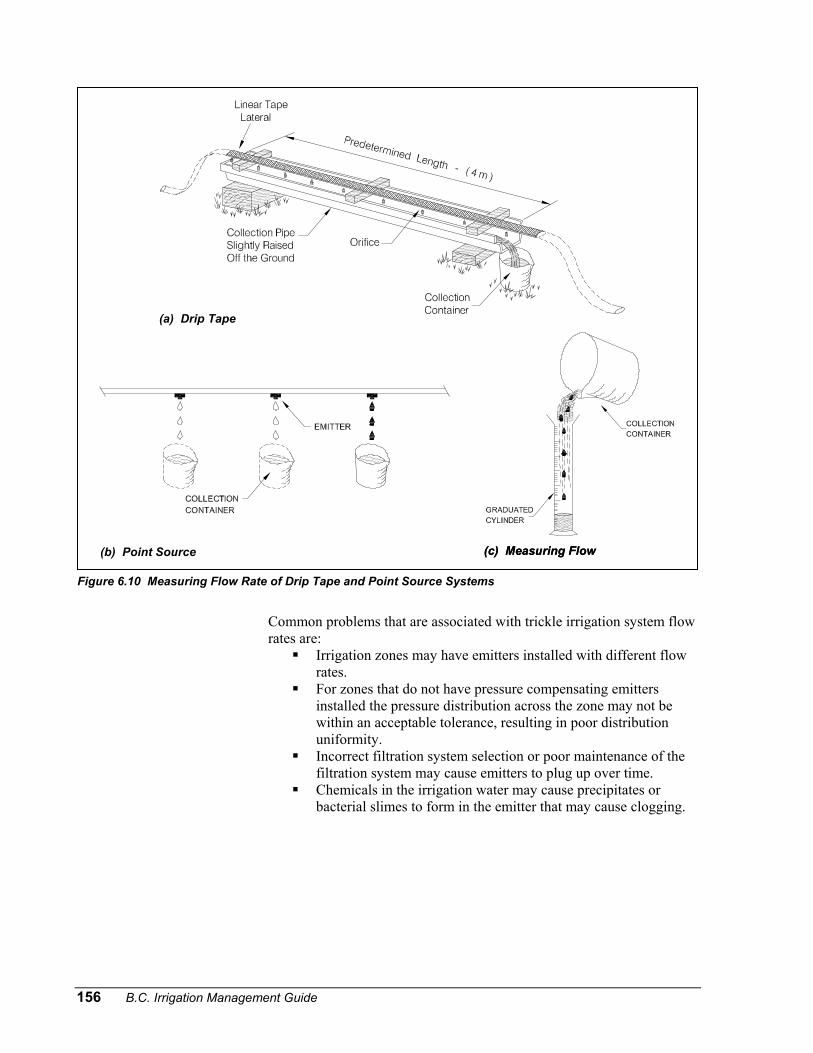
156 B.C. Irrigation Management Guide
Common problems that are associated with trickle irrigation system flow rates are:
Irrigation zones may have emitters installed with different flow rates.
For zones that do not have pressure compensating emitters installed the pressure distribution across the zone may not be within an acceptable tolerance, resulting in poor distribution uniformity.
Incorrect filtration system selection or poor maintenance of the filtration system may cause emitters to plug up over time.
Chemicals in the irrigation water may cause precipitates or bacterial slimes to form in the emitter that may cause clogging.
Figure 6.10 Measuring Flow Rate of Drip Tape and Point Source Systems
(a) Drip Tape
(b) Point Source (c) Measuring Flow (c) Measuring Flow
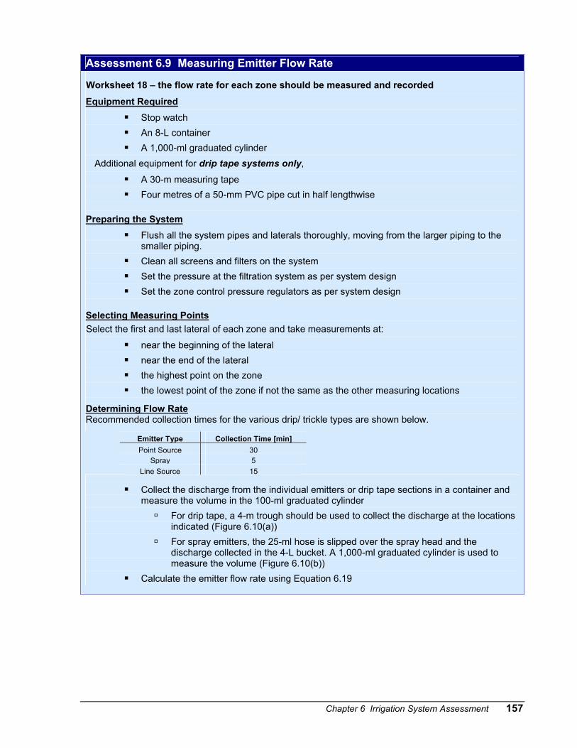
Chapter 6 Irrigation System Assessment 157
Assessment 6.9 Measuring Emitter Flow Rate
Worksheet 18 – the flow rate for each zone should be measured and recorded
Equipment Required Stop watch An 8-L container A 1,000-ml graduated cylinder
Additional equipment for drip tape systems only,
A 30-m measuring tape Four metres of a 50-mm PVC pipe cut in half lengthwise
Preparing the System Flush all the system pipes and laterals thoroughly, moving from the larger piping to the
smaller piping. Clean all screens and filters on the system Set the pressure at the filtration system as per system design Set the zone control pressure regulators as per system design
Selecting Measuring Points Select the first and last lateral of each zone and take measurements at:
near the beginning of the lateral near the end of the lateral the highest point on the zone the lowest point of the zone if not the same as the other measuring locations
Determining Flow Rate Recommended collection times for the various drip/ trickle types are shown below.
Emitter Type Collection Time [min]Point Source 30
Spray 5Line Source 15
Collect the discharge from the individual emitters or drip tape sections in a container and measure the volume in the 100-ml graduated cylinder
For drip tape, a 4-m trough should be used to collect the discharge at the locations indicated (Figure 6.10(a))
For spray emitters, the 25-ml hose is slipped over the spray head and the discharge collected in the 4-L bucket. A 1,000-ml graduated cylinder is used to measure the volume (Figure 6.10(b))
Calculate the emitter flow rate using Equation 6.19
158 B.C. Irrigation Management Guide
Actions for Worksheet 18 – Emitter Flow Rate Check
Action items that can solve problems with flow rates are:
Maintain the filtration system more regularly if emitters are plugged or flow rates have reduced. If there are algae, bacterial slimes or precipitates forming at the emitter. Check the B.C. Trickle
Irrigation Manual for methods of treating the water. B.C. Trickle Irrigation Manual
Flush the lateral lines more frequently. Check to see if the water temperature increases dramatically along the lateral line. Consider
burying or covering the lateral with mulch if the temperature increase is causing the emitter flow rate to change dramatically. In the B.C. Trickle Irrigation Manual, Table 4.2 provides information on flow changes due to temperature increases for various emitter types.
Emitter Spacing Check
The lateral line spacing is usually determined by the row spacing of the crop. In some instances, often on very sandy soils, more than one lateral may be required for the crop. In these situations, the lateral line spacing will be closer than the row spacing. See the B.C. Trickle Irrigation Manual for additional information.
B.C. Trickle Irrigation Manual
The emitter spacing is determined by the plant spacing, the plant root zone and the soil type. The emitters should be spaced close enough to ensure that at least 60% of the plant root zone is irrigated. The crop rooting area and the type of soil will often determine the number of emitters required. The emitter spacing check is done to determine if the crop rooting area is getting enough water and also to determine how much water is being delivered to the plants for a given set time. The number of emitters per plant in the field must be determined by measuring a section of lateral line and counting the number of plants and the number of emitters on the lateral line, or the number of discharge orifices if a drip tape system has been used. See Assessment 6.10. The number of emitters that should be installed per plant depends on:
the soil type and the wetting pattern that is developed by an emitter
the operating time for the zone, as longer operating times may increase the wetted area for each emitter
the emitter flow rate the crop rooting area and the plant spacing
Table 6.10 provides guidance on the minimum number of emitters that should be used per plant. For coarser soils extra emitters may be required.
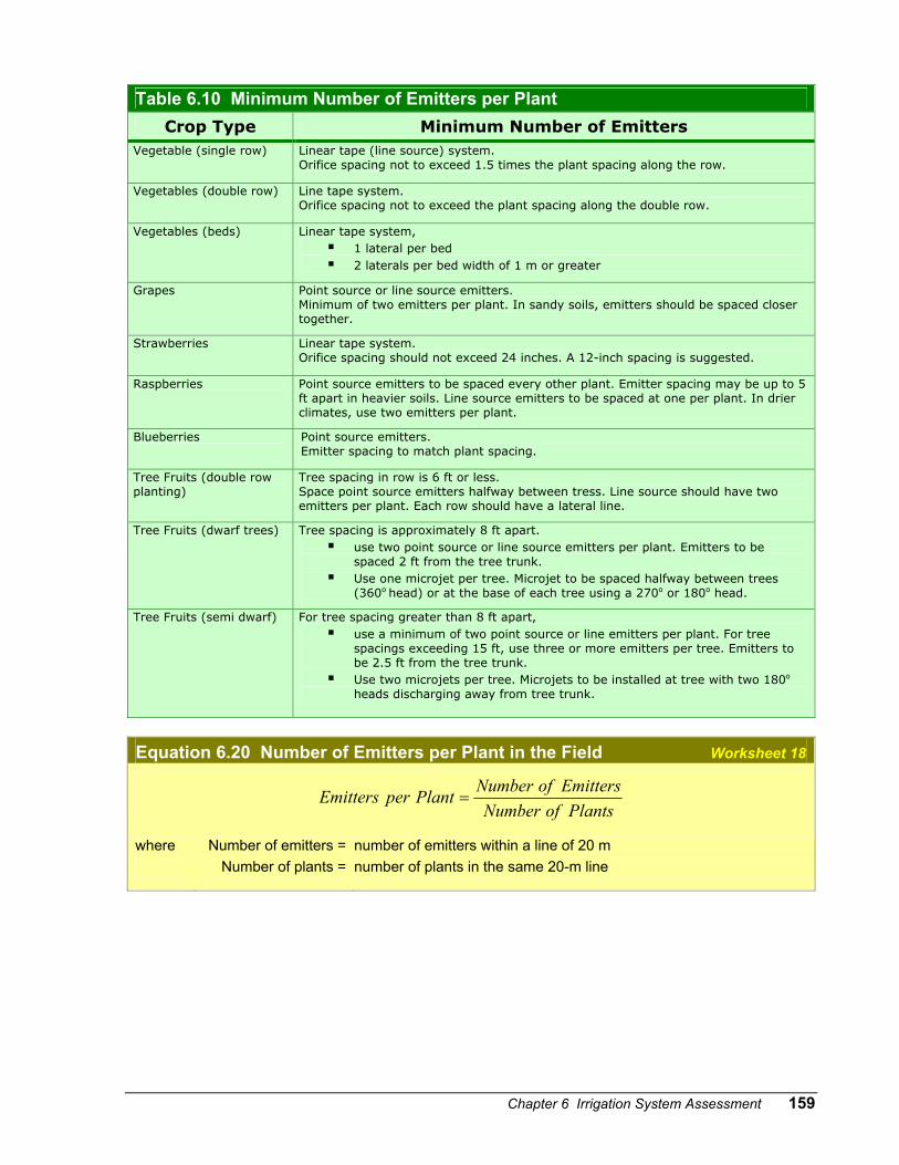
Chapter 6 Irrigation System Assessment 159
Table 6.10 Minimum Number of Emitters per Plant Crop Type Minimum Number of Emitters
Vegetable (single row) Linear tape (line source) system. Orifice spacing not to exceed 1.5 times the plant spacing along the row.
Vegetables (double row) Line tape system. Orifice spacing not to exceed the plant spacing along the double row.
Vegetables (beds) Linear tape system, 1 lateral per bed 2 laterals per bed width of 1 m or greater
Grapes Point source or line source emitters. Minimum of two emitters per plant. In sandy soils, emitters should be spaced closer together.
Strawberries Linear tape system. Orifice spacing should not exceed 24 inches. A 12-inch spacing is suggested.
Raspberries Point source emitters to be spaced every other plant. Emitter spacing may be up to 5 ft apart in heavier soils. Line source emitters to be spaced at one per plant. In drier climates, use two emitters per plant.
Blueberries Point source emitters. Emitter spacing to match plant spacing.
Tree Fruits (double row planting)
Tree spacing in row is 6 ft or less. Space point source emitters halfway between tress. Line source should have two emitters per plant. Each row should have a lateral line.
Tree Fruits (dwarf trees) Tree spacing is approximately 8 ft apart. use two point source or line source emitters per plant. Emitters to be
spaced 2 ft from the tree trunk. Use one microjet per tree. Microjet to be spaced halfway between trees
(360o head) or at the base of each tree using a 270o or 180o head.
Tree Fruits (semi dwarf) For tree spacing greater than 8 ft apart, use a minimum of two point source or line emitters per plant. For tree
spacings exceeding 15 ft, use three or more emitters per tree. Emitters to be 2.5 ft from the tree trunk.
Use two microjets per tree. Microjets to be installed at tree with two 180o heads discharging away from tree trunk.
Equation 6.20 Number of Emitters per Plant in the Field Worksheet 18
PlantsofNumberEmittersofNumberPlantperEmitters =
where
Number of emitters = Number of plants =
number of emitters within a line of 20 m number of plants in the same 20-m line
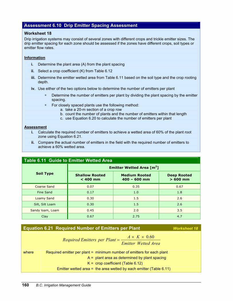
160 B.C. Irrigation Management Guide
Assessment 6.10 Drip Emitter Spacing Assessment
Worksheet 18 Drip irrigation systems may consist of several zones with different crops and trickle emitter sizes. The drip emitter spacing for each zone should be assessed if the zones have different crops, soil types or emitter flow rates. Information
i. Determine the plant area (A) from the plant spacing
ii. Select a crop coefficient (K) from Table 6.12
iii. Determine the emitter wetted area from Table 6.11 based on the soil type and the crop rooting depth.
iv. Use either of the two options below to determine the number of emitters per plant
Determine the number of emitters per plant by dividing the plant spacing by the emitter spacing.
For closely spaced plants use the following method: a. take a 20-m section of a crop row b. count the number of plants and the number of emitters within that length c. use Equation 6.20 to calculate the number of emitters per plant
Assessment
i. Calculate the required number of emitters to achieve a wetted area of 60% of the plant root zone using Equation 6.21.
ii. Compare the actual number of emitters in the field with the required number of emitters to achieve a 60% wetted area.
Table 6.11 Guide to Emitter Wetted Area
Emitter Wetted Area [m2] Soil Type Shallow Rooted
< 400 mm Medium Rooted 400 – 600 mm
Deep Rooted > 600 mm
Coarse Sand 0.07 0.35 0.67
Fine Sand 0.17 1.0 1.8
Loamy Sand 0.30 1.5 2.6
Silt, Silt Loam 0.30 1.5 2.6
Sandy loam, Loam 0.45 2.0 3.5
Clay 0.67 2.75 4.7
Equation 6.21 Required Number of Emitters per Plant Worksheet 18
AreaWettedEmitterKAPlantperEmittersequiredR 60.0××
=
where
Required emitter per plant = A = K =
Emitter wetted area =
minimum number of emitters for each plant plant area as determined by plant spacing crop coefficient (Table 6.12) the area wetted by each emitter (Table 6.11)
Chapter 6 Irrigation System Assessment 161
Actions for Worksheet 18 – Emitter Spacing Check
To ensure peak performance from the drip system:
Ensure that each plant in a zone has the same number of emitters. Ensure that the emitter wetted area covers at least 60% of the crop root zone. If this is not
possible with one lateral an additional lateral should be added. For row crops ensure that the wetted pattern from the emitter reaches the wetted pattern from
the next emitter to ensure uniform application is occurring.
Pressure Distribution Check (Optional) The pressure distribution check does not need to be done if the emitter flow rates throughout the system are uniform (i.e., within 10% difference compared to the emitter flow rate stated by the supplier). If the flow is not uniform, the pressure distribution check will help determine if the system design or product selection are a cause of the flow variation. Pressure distribution can have a big impact on trickle system uniformity and performance, especially if pressure compensating emitters are not used. If flow rates are uneven throughout a zone, it is very difficult to manage the system to make efficient use of water resources. In these cases, it is inevitable that some parts of the field are over-irrigated while others are under-irrigated. Each irrigation zone should be assessed separately for pressure distribution uniformity. The best method is to have pressure monitoring stations installed in key locations on the system. The best locations are the same as those used for monitoring flow rates. See Assessment 6.9. A pressure gauge can then be installed as needed to monitor the pressure. The maximum pressure variation throughout a zone should not exceed:
10% for laminar flow emitters 20% for turbulent flow emitters
Refer to the B.C. Trickle Irrigation Manual for procedures and information on how to determine distribution uniformity in a trickle system.
B.C. Trickle Irrigation Manual
162 B.C. Irrigation Management Guide
Actions for Worksheet 18 – Pressure Distribution Check
Action items to correct pressure distribution problems are:
Check the pressure at the zone control valve to ensure proper pressure is provided at the start of the zone.
Feed the irrigation lateral from both ends if the pressure loss along the lateral is too great. Divide the zones into smaller areas to allow for better pressure control. If the laterals are running uphill from the submain, move the submain to the other end of the
laterals, allowing them to run downhill. Flush laterals to ensure best system performance Consider using pressure compensating emitters if nothing else works.
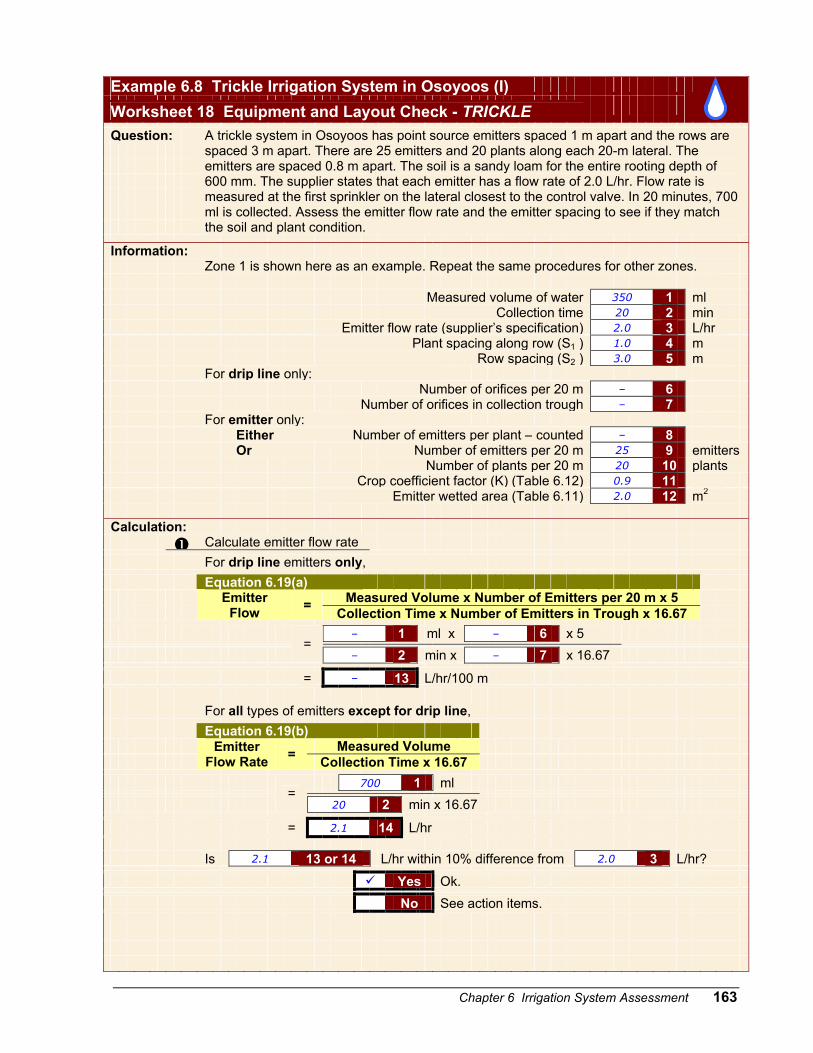
Chapter 6 Irrigation System Assessment 163
Example 6.8 Trickle Irrigation System in Osoyoos (I)
Worksheet 18 Equipment and Layout Check - TRICKLE
Question:
A trickle system in Osoyoos has point source emitters spaced 1 m apart and the rows are spaced 3 m apart. There are 25 emitters and 20 plants along each 20-m lateral. The emitters are spaced 0.8 m apart. The soil is a sandy loam for the entire rooting depth of 600 mm. The supplier states that each emitter has a flow rate of 2.0 L/hr. Flow rate is measured at the first sprinkler on the lateral closest to the control valve. In 20 minutes, 700 ml is collected. Assess the emitter flow rate and the emitter spacing to see if they match the soil and plant condition.
Information: Zone 1 is shown here as an example. Repeat the same procedures for other zones. Measured volume of water 350 1 ml Collection time 20 2 min Emitter flow rate (supplier’s specification) 2.0 3 L/hr Plant spacing along row (S1 ) 1.0 4 m Row spacing (S2 ) 3.0 5 m For drip line only: Number of orifices per 20 m – 6 Number of orifices in collection trough – 7 For emitter only: Either Number of emitters per plant – counted – 8 Or Number of emitters per 20 m 25 9 emitters Number of plants per 20 m 20 10 plants Crop coefficient factor (K) (Table 6.12) 0.9 11 Emitter wetted area (Table 6.11) 2.0 12 m2
Calculation: Calculate emitter flow rate For drip line emitters only, Equation 6.19(a) Measured Volume x Number of Emitters per 20 m x 5
Emitter Flow = Collection Time x Number of Emitters in Trough x 16.67
– 1 ml x – 6 x 5
= – 2 min x – 7 x 16.67
= – 13 L/hr/100 m For all types of emitters except for drip line, Equation 6.19(b) Measured Volume
Emitter Flow Rate = Collection Time x 16.67
700 1 ml
= 20 2 min x 16.67
= 2.1 14 L/hr Is 2.1 13 or 14 L/hr within 10% difference from 2.0 3 L/hr?
Yes Ok. No See action items.
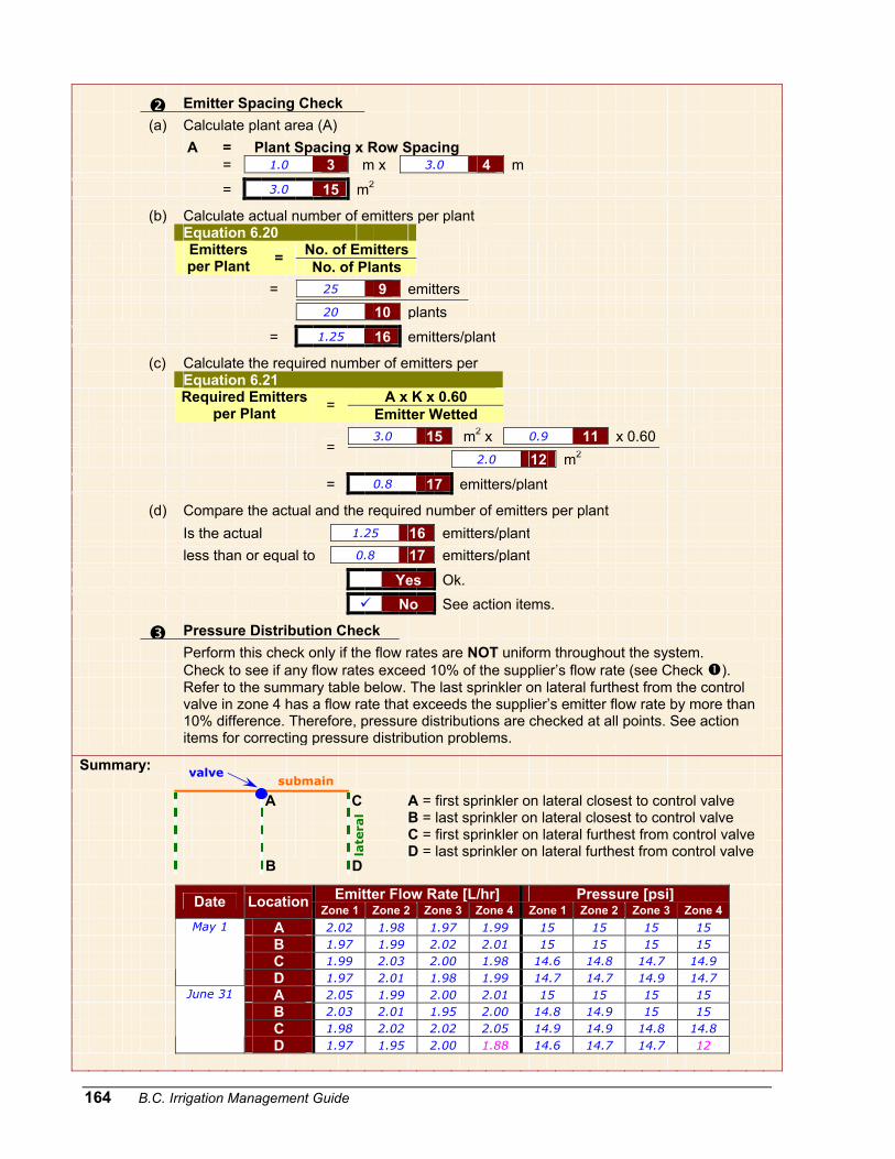
164 B.C. Irrig
Emitter Spacing Check (a) Calculate plant area (A) A = Plant Spacing x Row Spacing = 1.0 3 m x 3.0 4 m
= 3.0 15 m2
(b) Calculate actual number of emitters per plant Equation 6.20 No. of Emitters
Emitters per Plant = No. of Plants
25 9 emitters
= 20 10 plants
= 1.25 16 emitters/plant
(c) Calculate the required number of emitters per Equation 6.21 A x K x 0.60
Required Emitters per Plant = Emitter Wetted
3.0 15 m2 x 0.9 11 x 0.60
= 2.0 12 m2
= 0.8 17 emitters/plant
(d) Compare the actual and the required number of emitters per plant Is the actual 1.25 16 emitters/plant less than or equal to 0.8 17 emitters/plant
Yes Ok. No See action items.
Pressure Distribution Check
Perform this check only if the flow rates are NOT uniform throughout the system. Check to see if any flow rates exceed 10% of the supplier’s flow rate (see Check ). Refer to the summary table below. The last sprinkler on lateral furthest from the control valve in zone 4 has a flow rate that exceeds the supplier’s emitter flow rate by more than 10% difference. Therefore, pressure distributions are checked at all points. See action items for correcting pressure distribution problems.
Summary:
J
valveation Management Guide
A C
A = first sprinkler on lateral closest to control valve B = last sprinkler on lateral closest to control valve C = first sprinkler on lateral furthest from control valve D = last sprinkler on lateral furthest from control valve
B D
Emitter Flow Rate [L/hr] Pressure [psi] Date Location Zone 1 Zone 2 Zone 3 Zone 4 Zone 1 Zone 2 Zone 3 Zone 4 A 2.02 1.98 1.97 1.99 15 15 15 15
B 1.97 1.99 2.02 2.01 15 15 15 15
C 1.99 2.03 2.00 1.98 14.6 14.8 14.7 14.9
May 1
D 1.97 2.01 1.98 1.99 14.7 14.7 14.9 14.7
A 2.05 1.99 2.00 2.01 15 15 15 15
B 2.03 2.01 1.95 2.00 14.8 14.9 15 15
C 1.98 2.02 2.02 2.05 14.9 14.9 14.8 14.8
une 31
D 1.97 1.95 2.00 1.88 14.6 14.7 14.7 12
submain
late
ral
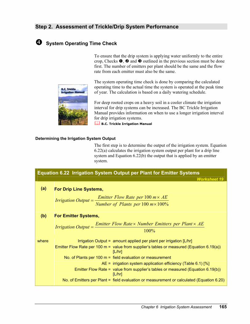
Chapter 6 Irrigation System Assessment 165
Step 2. Assessment of Trickle/Drip System Performance
System Operating Time Check
To ensure that the drip system is applying water uniformly to the entire crop, Checks , and outlined in the previous section must be done first. The number of emitters per plant should be the same and the flow rate from each emitter must also be the same. The system operating time check is done by comparing the calculated operating time to the actual time the system is operated at the peak time of year. The calculation is based on a daily watering schedule. For deep rooted crops on a heavy soil in a cooler climate the irrigation interval for drip systems can be increased. The BC Trickle Irrigation Manual provides information on when to use a longer irrigation interval for drip irrigation systems.
B.C. Trickle Irrigation Manual
Determining the Irrigation System Output The first step is to determine the output of the irrigation system. Equation 6.22(a) calculates the irrigation system output per plant for a drip line system and Equation 6.22(b) the output that is applied by an emitter system.
Equation 6.22 Irrigation System Output per Plant for Emitter Systems Worksheet 19
(a)
For Drip Line Systems,
%100100100
××
=mperPlantsofNumber
AEmperRateFlowEmitterOutputIrrigation
(b) For Emitter Systems,
%100AEPlantperEmittersNumberRateFlowEmitterOutputIrrigation ××
=
where
Irrigation Output = Emitter Flow Rate per 100 m =
No. of Plants per 100 m =
AE = Emitter Flow Rate =
No. of Emitters per Plant =
amount applied per plant per irrigation [L/hr] value from supplier’s tables or measured (Equation 6.19(a)) [L/hr] field evaluation or measurement irrigation system application efficiency (Table 6.1) [%] value from supplier’s tables or measured (Equation 6.19(b)) [L/hr] field evaluation or measurement or calculated (Equation 6.20)
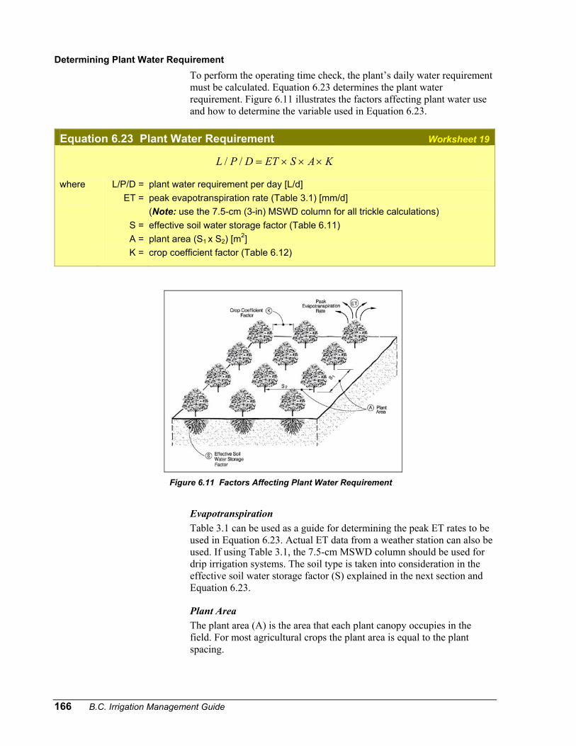
166 B.C. Irrigation Management Guide
Determining Plant Water Requirement To perform the operating time check, the plant’s daily water requirement must be calculated. Equation 6.23 determines the plant water requirement. Figure 6.11 illustrates the factors affecting plant water use and how to determine the variable used in Equation 6.23.
Equation 6.23 Plant Water Requirement Worksheet 19
KASETDPL ×××=//
where
L/P/D = ET =
S = A = K =
plant water requirement per day [L/d] peak evapotranspiration rate (Table 3.1) [mm/d] (Note: use the 7.5-cm (3-in) MSWD column for all trickle calculations) effective soil water storage factor (Table 6.11) plant area (S1 x S2) [m2] crop coefficient factor (Table 6.12)
Evapotranspiration Table 3.1 can be used as a guide for determining the peak ET rates to be used in Equation 6.23. Actual ET data from a weather station can also be used. If using Table 3.1, the 7.5-cm MSWD column should be used for drip irrigation systems. The soil type is taken into consideration in the effective soil water storage factor (S) explained in the next section and Equation 6.23.
Plant Area The plant area (A) is the area that each plant canopy occupies in the field. For most agricultural crops the plant area is equal to the plant spacing.
Figure 6.11 Factors Affecting Plant Water Requirement
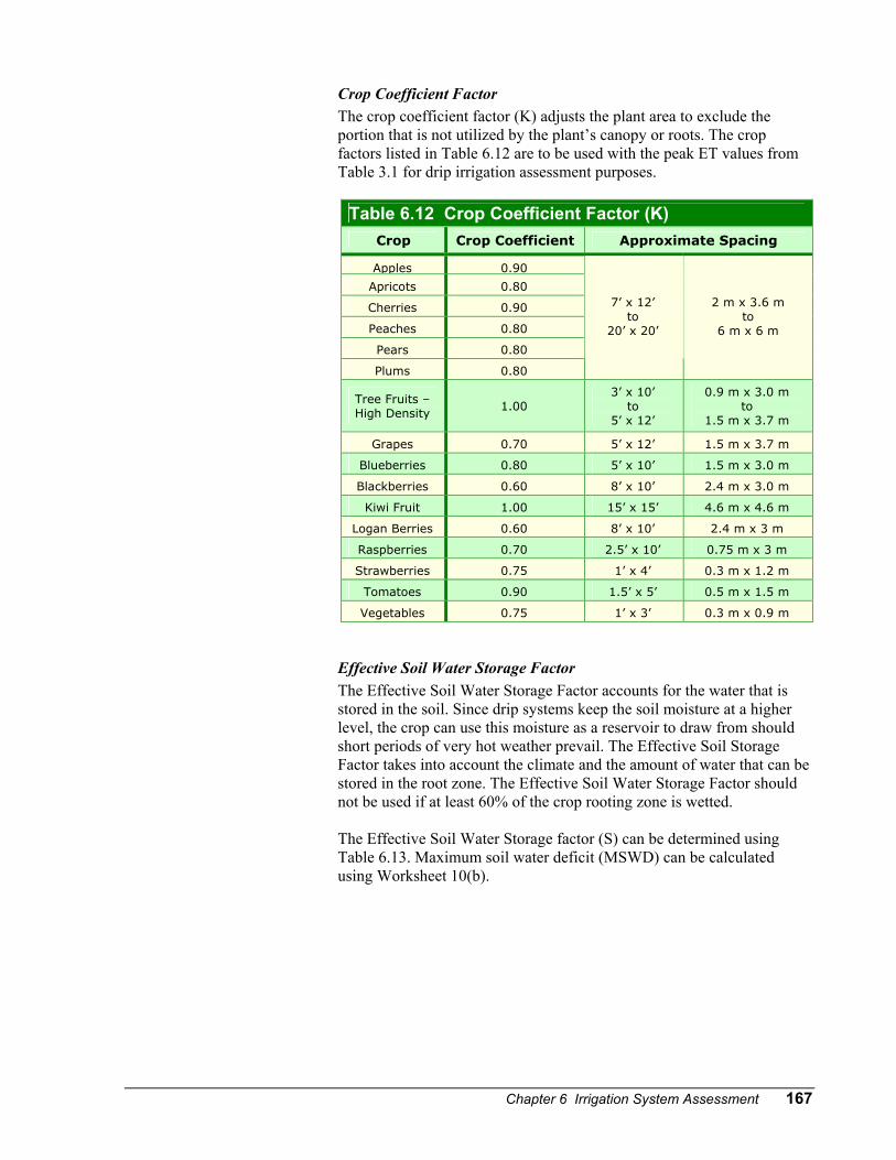
Chapter 6 Irrigation System Assessment 167
Crop Coefficient Factor The crop coefficient factor (K) adjusts the plant area to exclude the portion that is not utilized by the plant’s canopy or roots. The crop factors listed in Table 6.12 are to be used with the peak ET values from Table 3.1 for drip irrigation assessment purposes.
Table 6.12 Crop Coefficient Factor (K) Crop Crop Coefficient Approximate Spacing
Apples 0.90
Apricots 0.80
Cherries 0.90
Peaches 0.80
Pears 0.80
Plums 0.80
7’ x 12’ to
20’ x 20’
2 m x 3.6 m to
6 m x 6 m
Tree Fruits – High Density
1.00 3’ x 10’
to 5’ x 12’
0.9 m x 3.0 m to
1.5 m x 3.7 m
Grapes 0.70 5’ x 12’ 1.5 m x 3.7 m
Blueberries 0.80 5’ x 10’ 1.5 m x 3.0 m
Blackberries 0.60 8’ x 10’ 2.4 m x 3.0 m
Kiwi Fruit 1.00 15’ x 15’ 4.6 m x 4.6 m
Logan Berries 0.60 8’ x 10’ 2.4 m x 3 m
Raspberries 0.70 2.5’ x 10’ 0.75 m x 3 m
Strawberries 0.75 1’ x 4’ 0.3 m x 1.2 m
Tomatoes 0.90 1.5’ x 5’ 0.5 m x 1.5 m
Vegetables 0.75 1’ x 3’ 0.3 m x 0.9 m
Effective Soil Water Storage Factor The Effective Soil Water Storage Factor accounts for the water that is stored in the soil. Since drip systems keep the soil moisture at a higher level, the crop can use this moisture as a reservoir to draw from should short periods of very hot weather prevail. The Effective Soil Storage Factor takes into account the climate and the amount of water that can be stored in the root zone. The Effective Soil Water Storage Factor should not be used if at least 60% of the crop rooting zone is wetted. The Effective Soil Water Storage factor (S) can be determined using Table 6.13. Maximum soil water deficit (MSWD) can be calculated using Worksheet 10(b).
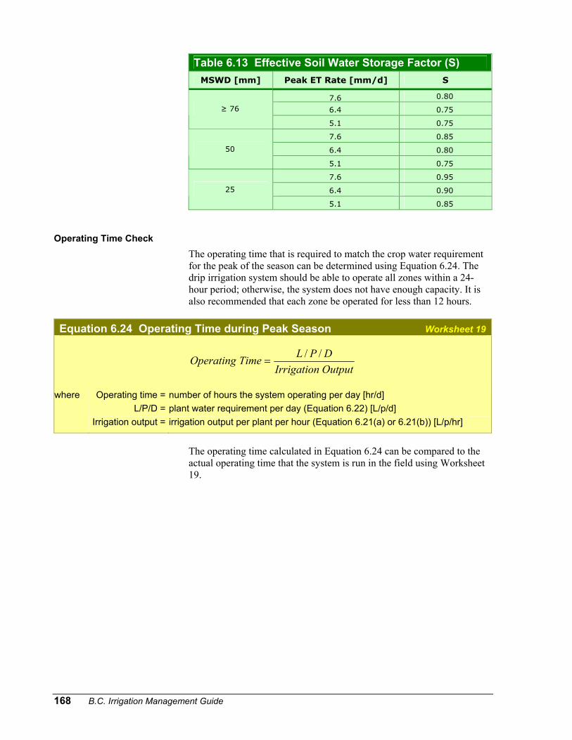
168 B.C. Irrigation Management Guide
Table 6.13 Effective Soil Water Storage Factor (S) MSWD [mm] Peak ET Rate [mm/d] S
7.6 0.80
6.4 0.75 ≥ 76
5.1 0.75
7.6 0.85
6.4 0.80 50
5.1 0.75
7.6 0.95
6.4 0.90 25
5.1 0.85
Operating Time Check The operating time that is required to match the crop water requirement for the peak of the season can be determined using Equation 6.24. The drip irrigation system should be able to operate all zones within a 24-hour period; otherwise, the system does not have enough capacity. It is also recommended that each zone be operated for less than 12 hours.
Equation 6.24 Operating Time during Peak Season Worksheet 19
OutputIrrigationDPLTimeOperating //
=
where
Operating time = L/P/D =
Irrigation output =
number of hours the system operating per day [hr/d] plant water requirement per day (Equation 6.22) [L/p/d] irrigation output per plant per hour (Equation 6.21(a) or 6.21(b)) [L/p/hr]
The operating time calculated in Equation 6.24 can be compared to the actual operating time that the system is run in the field using Worksheet 19.
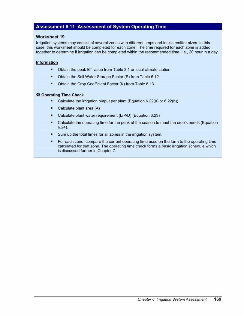
Chapter 6 Irrigation System Assessment 169
Assessment 6.11 Assessment of System Operating Time Worksheet 19 Irrigation systems may consist of several zones with different crops and trickle emitter sizes. In this case, this worksheet should be completed for each zone. The time required for each zone is added together to determine if irrigation can be completed within the recommended time, i.e., 20 hour in a day. Information
Obtain the peak ET value from Table 3.1 or local climate station.
Obtain the Soil Water Storage Factor (S) from Table 6.12.
Obtain the Crop Coefficient Factor (K) from Table 6.13.
Operating Time Check Calculate the irrigation output per plant (Equation 6.22(a) or 6.22(b))
Calculate plant area (A)
Calculate plant water requirement (L/P/D) (Equation 6.23)
Calculate the operating time for the peak of the season to meet the crop’s needs (Equation 6.24).
Sum up the total times for all zones in the irrigation system.
For each zone, compare the current operating time used on the farm to the operating time calculated for that zone. The operating time check forms a basic irrigation schedule which is discussed further in Chapter 7.
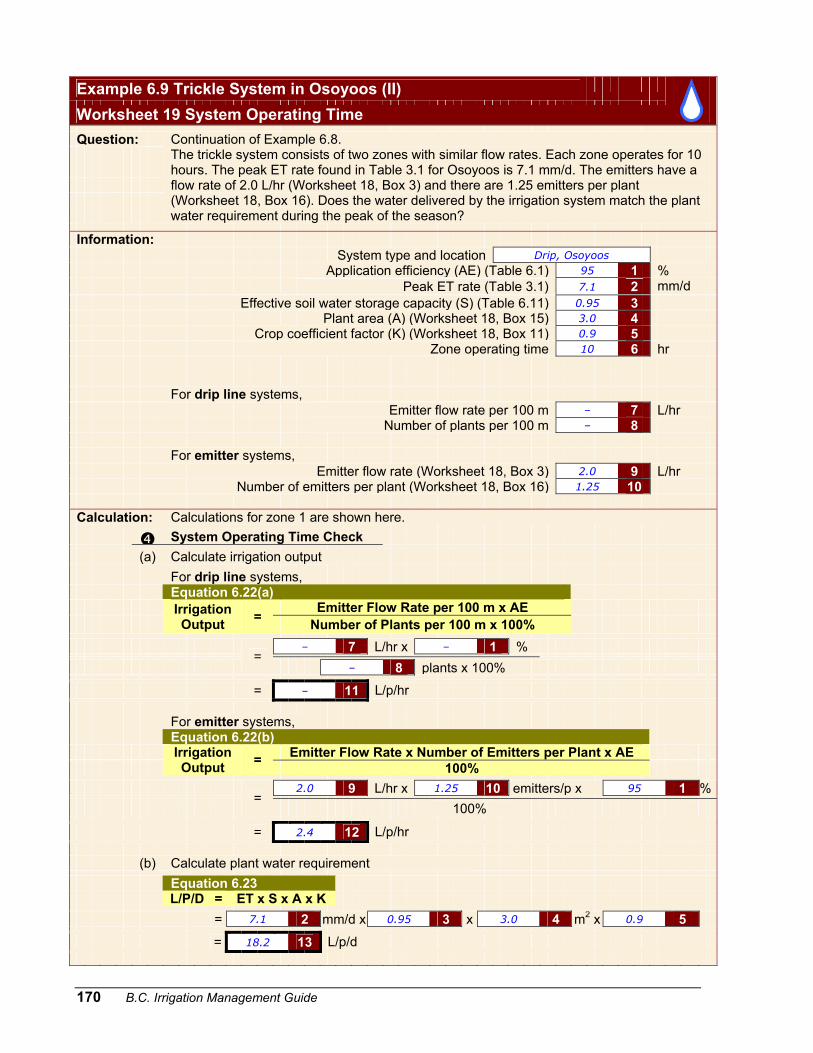
170 B.C. Irrigation Management Guide
Example 6.9 Trickle System in Osoyoos (II)
Worksheet 19 System Operating Time
Question:
Continuation of Example 6.8. The trickle system consists of two zones with similar flow rates. Each zone operates for 10 hours. The peak ET rate found in Table 3.1 for Osoyoos is 7.1 mm/d. The emitters have a flow rate of 2.0 L/hr (Worksheet 18, Box 3) and there are 1.25 emitters per plant (Worksheet 18, Box 16). Does the water delivered by the irrigation system match the plant water requirement during the peak of the season?
Information: System type and location Drip, Osoyoos
Application efficiency (AE) (Table 6.1) 95 1 % Peak ET rate (Table 3.1) 7.1 2 mm/d Effective soil water storage capacity (S) (Table 6.11) 0.95 3 Plant area (A) (Worksheet 18, Box 15) 3.0 4 Crop coefficient factor (K) (Worksheet 18, Box 11) 0.9 5 Zone operating time 10 6 hr For drip line systems, Emitter flow rate per 100 m – 7 L/hr Number of plants per 100 m – 8 For emitter systems, Emitter flow rate (Worksheet 18, Box 3) 2.0 9 L/hr Number of emitters per plant (Worksheet 18, Box 16) 1.25 10 Calculation: Calculations for zone 1 are shown here. System Operating Time Check (a) Calculate irrigation output For drip line systems, Equation 6.22(a) Emitter Flow Rate per 100 m x AE
Irrigation Output = Number of Plants per 100 m x 100%
– 7 L/hr x – 1 %
= – 8 plants x 100%
= – 11 L/p/hr For emitter systems, Equation 6.22(b) Emitter Flow Rate x Number of Emitters per Plant x AE
Irrigation Output = 100%
2.0 9 L/hr x 1.25 10 emitters/p x 95 1 %
= 100%
= 2.4 12 L/p/hr (b) Calculate plant water requirement Equation 6.23 L/P/D = ET x S x A x K = 7.1 2 mm/d x 0.95 3 x 3.0 4 m2 x 0.9 5 = 18.2 13 L/p/d
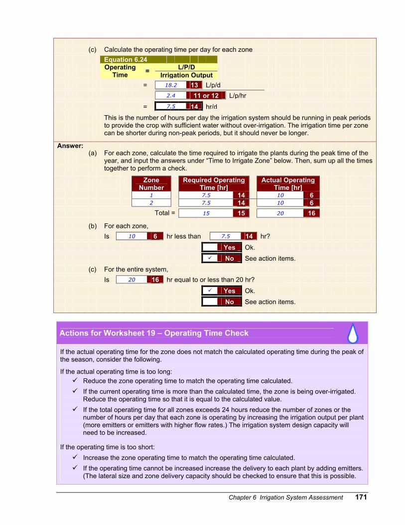
Chapter 6 Irrigation System Assessment 171
(c) Calculate the operating time per day for each zone Equation 6.24 L/P/D
Operating Time = Irrigation Output
18.2 13 L/p/d
= 2.4 11 or 12 L/p/hr
= 7.5 14 hr/d
This is the number of hours per day the irrigation system should be running in peak periods to provide the crop with sufficient water without over-irrigation. The irrigation time per zone can be shorter during non-peak periods, but it should never be longer.
Answer: (a)
For each zone, calculate the time required to irrigate the plants during the peak time of the year, and input the answers under “Time to Irrigate Zone” below. Then, sum up all the times together to perform a check.
Zone Number
Required Operating Time [hr]
Actual Operating Time [hr]
1 7.5 14 10 6 2 7.5 14 10 6 Total = 15 15 20 16
(b) For each zone, Is 10 6 hr less than 7.5 14 hr?
Yes Ok. No See action items. (c) For the entire system, Is 20 16 hr equal to or less than 20 hr?
Yes Ok. No See action items.
Actions for Worksheet 19 – Operating Time Check
If the actual operating time for the zone does not match the calculated operating time during the peak of the season, consider the following.
If the actual operating time is too long: Reduce the zone operating time to match the operating time calculated. If the current operating time is more than the calculated time, the zone is being over-irrigated.
Reduce the operating time so that it is equal to the calculated value. If the total operating time for all zones exceeds 24 hours reduce the number of zones or the
number of hours per day that each zone is operating by increasing the irrigation output per plant (more emitters or emitters with higher flow rates.) The irrigation system design capacity will need to be increased.
If the operating time is too short: Increase the zone operating time to match the operating time calculated. If the operating time cannot be increased increase the delivery to each plant by adding emitters.
(The lateral size and zone delivery capacity should be checked to ensure that this is possible.

172 B.C. Irrigation Management Guide