Embed Size (px)
Citation preview
科学技術計算のためのマルチコアプログラミング入門
C言語編第Ⅰ部:概要,対象アプリケーション,OpenMP
中島研吾東京大学情報基盤センター
OMP-1 2
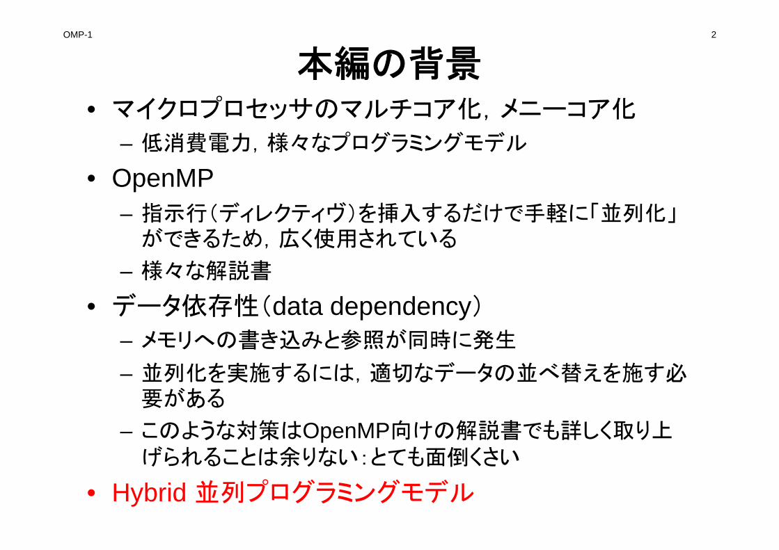
本編の背景• マイクロプロセッサのマルチコア化,メニーコア化
– 低消費電力,様々なプログラミングモデル
• OpenMP– 指示行(ディレクティヴ)を挿入するだけで手軽に「並列化」
ができるため,広く使用されている
– 様々な解説書
• データ依存性(data dependency)
– メモリへの書き込みと参照が同時に発生
– 並列化を実施するには,適切なデータの並べ替えを施す必要がある
– このような対策はOpenMP向けの解説書でも詳しく取り上げられることは余りない:とても面倒くさい
• Hybrid 並列プログラミングモデル
OMP-1 3
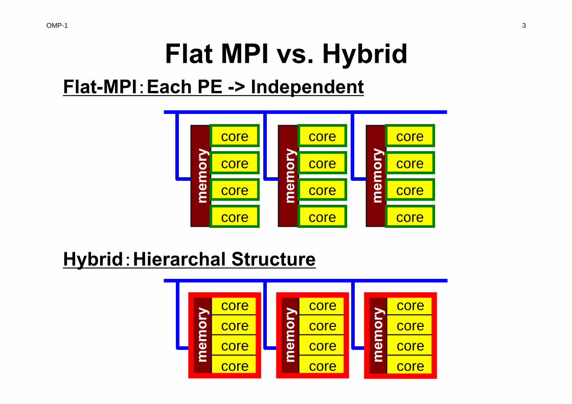
Flat MPI vs. Hybrid
Hybrid:Hierarchal Structure
Flat-MPI:Each PE -> Independent
corecorecorecorem
emor
y corecorecorecorem
emor
y corecorecorecorem
emor
y corecorecorecorem
emor
y corecorecorecorem
emor
y corecorecorecorem
emor
y
mem
ory
mem
ory
mem
ory
core
core
core
core
core
core
core
core
core
core
core
core
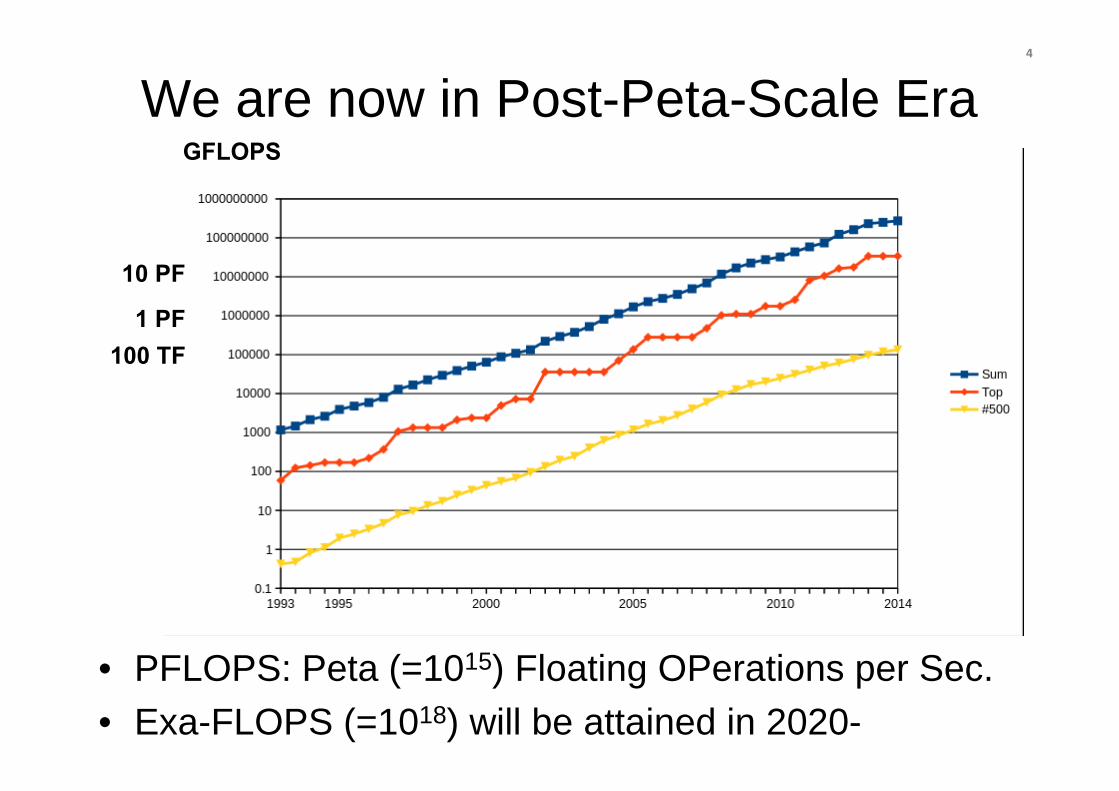
We are now in Post-Peta-Scale Era
• PFLOPS: Peta (=1015) Floating OPerations per Sec.• Exa-FLOPS (=1018) will be attained in 2020-
4
GFLOPS
10 PF
1 PF100 TF
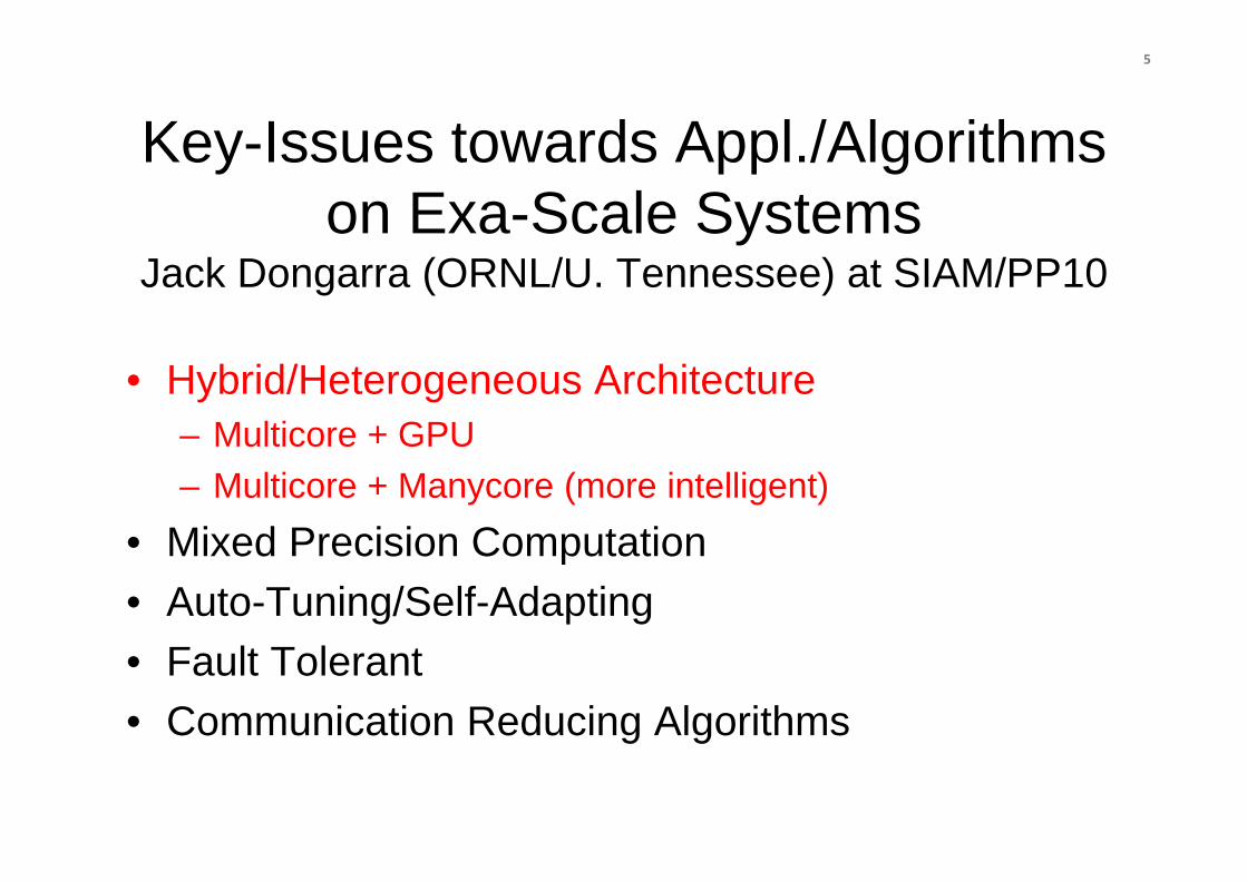
Key-Issues towards Appl./Algorithms on Exa-Scale Systems
Jack Dongarra (ORNL/U. Tennessee) at SIAM/PP10
• Hybrid/Heterogeneous Architecture– Multicore + GPU– Multicore + Manycore (more intelligent)
• Mixed Precision Computation• Auto-Tuning/Self-Adapting• Fault Tolerant• Communication Reducing Algorithms
5
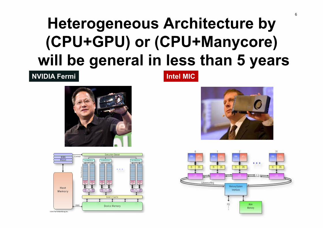
6
Heterogeneous Architecture by (CPU+GPU) or (CPU+Manycore)
will be general in less than 5 yearsIntel MICNVIDIA Fermi
7
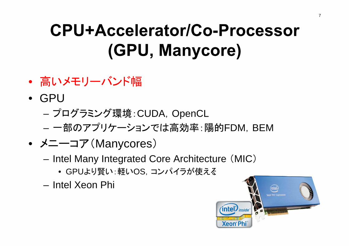
CPU+Accelerator/Co-Processor (GPU, Manycore)
• 高いメモリーバンド幅
• GPU– プログラミング環境:CUDA,OpenCL– 一部のアプリケーションでは高効率:陽的FDM,BEM
• メニーコア(Manycores)
– Intel Many Integrated Core Architecture (MIC)• GPUより賢い:軽いOS,コンパイラが使える
– Intel Xeon Phi
Hybrid並列プログラミングモデルは必須
• Message Passing– MPI
• Multi Threading– OpenMP, CUDA, OpenCL, OpenACC
• 「京」でもHybrid並列プログラミングモデルが推奨されている
– 但し MPI+自動並列化(ノード内)
8
OMP-1 9
本編の目的
• 「有限体積法から導かれる疎行列を対象としたICCG法」を題材とした,データ配置,reorderingなど,科学
技術計算のためのマルチコアプログラミングにおいて重要なアルゴリズムについての講習
• 更に理解を深めるための,FX10を利用した実習
• 単一のアプリケーションに特化した内容であるが,基本的な考え方は様々な分野に適用可能である
– 実はこの方法は意外に効果的である
OMP-1 10
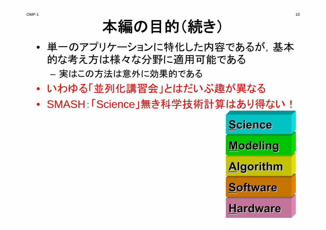
本編の目的(続き)• 単一のアプリケーションに特化した内容であるが,基本
的な考え方は様々な分野に適用可能である
– 実はこの方法は意外に効果的である
• いわゆる「並列化講習会」とはだいぶ趣が異なる
• SMASH:「Science」無き科学技術計算はあり得ない!
HHardwareardware
SSoftwareoftware
AAlgorithmlgorithm
MModelingodeling
SSciencecience
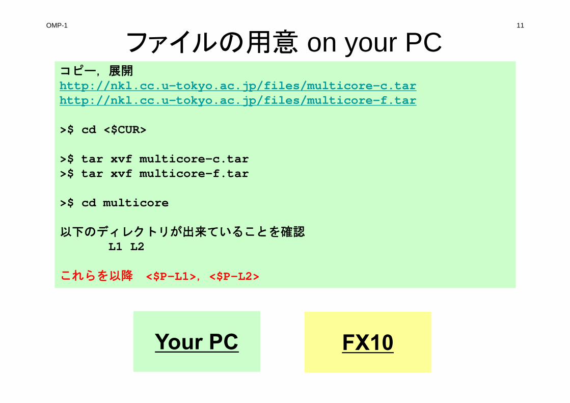
OMP-1 11
ファイルの用意 on your PCコピー,展開http://nkl.cc.u-tokyo.ac.jp/files/multicore-c.tarhttp://nkl.cc.u-tokyo.ac.jp/files/multicore-f.tar
>$ cd <$CUR>
>$ tar xvf multicore-c.tar>$ tar xvf multicore-f.tar
>$ cd multicore
以下のディレクトリが出来ていることを確認L1 L2
これらを以降 <$P-L1>,<$P-L2>
Your PC FX10
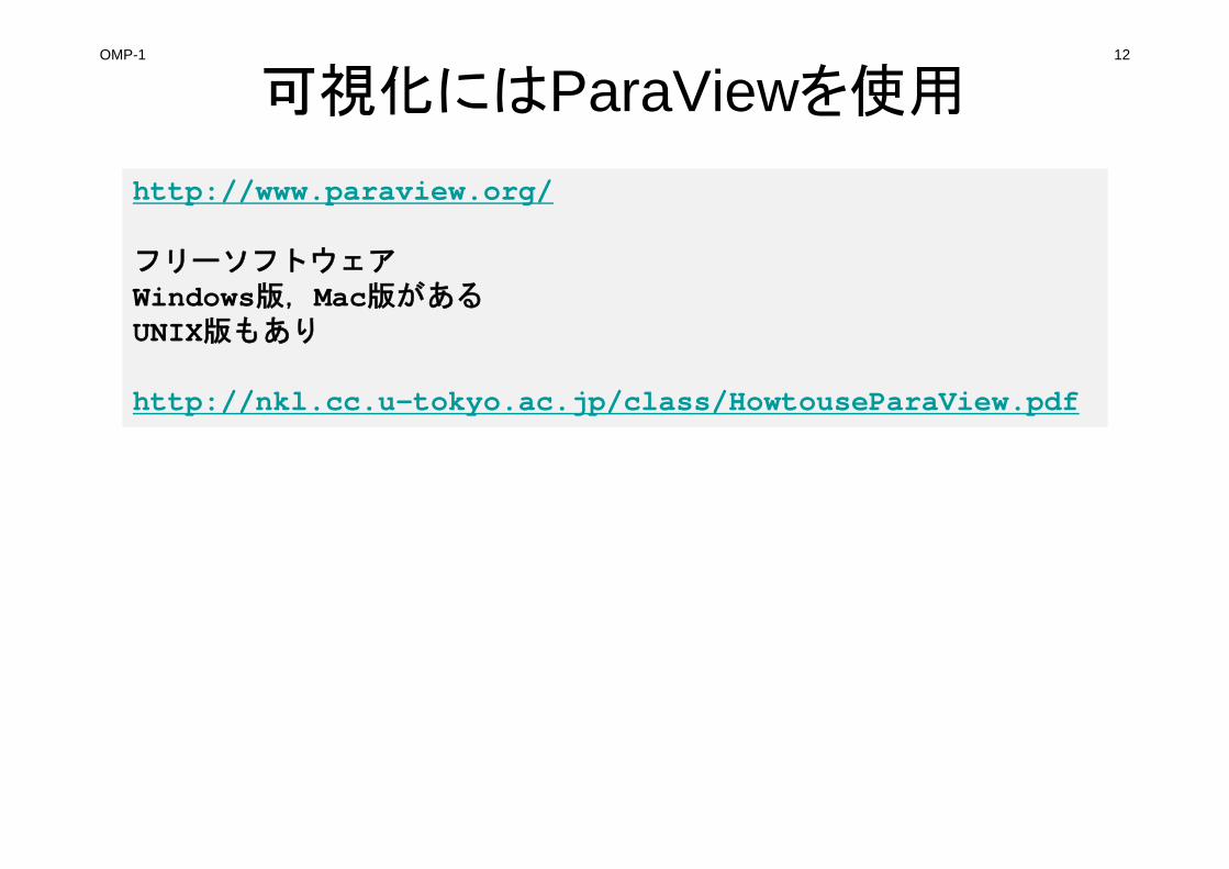
OMP-1 12
可視化にはParaViewを使用
http://www.paraview.org/
フリーソフトウェアWindows版,Mac版があるUNIX版もあり
http://nkl.cc.u-tokyo.ac.jp/class/HowtouseParaView.pdf

OMP-1 13
資料はWeb上にもあります
http://nkl.cc.u-tokyo.ac.jp/seminars/2015-Spring/
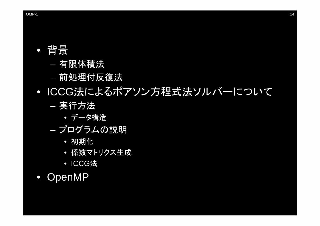
OMP-1 14
• 背景
– 有限体積法
– 前処理付反復法
• ICCG法によるポアソン方程式法ソルバーについて
– 実行方法• データ構造
– プログラムの説明• 初期化
• 係数マトリクス生成
• ICCG法
• OpenMP
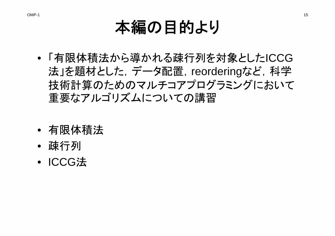
OMP-1 15
本編の目的より
• 「有限体積法から導かれる疎行列を対象としたICCG法」を題材とした,データ配置,reorderingなど,科学
技術計算のためのマルチコアプログラミングにおいて重要なアルゴリズムについての講習
• 有限体積法
• 疎行列
• ICCG法
OMP-1 16
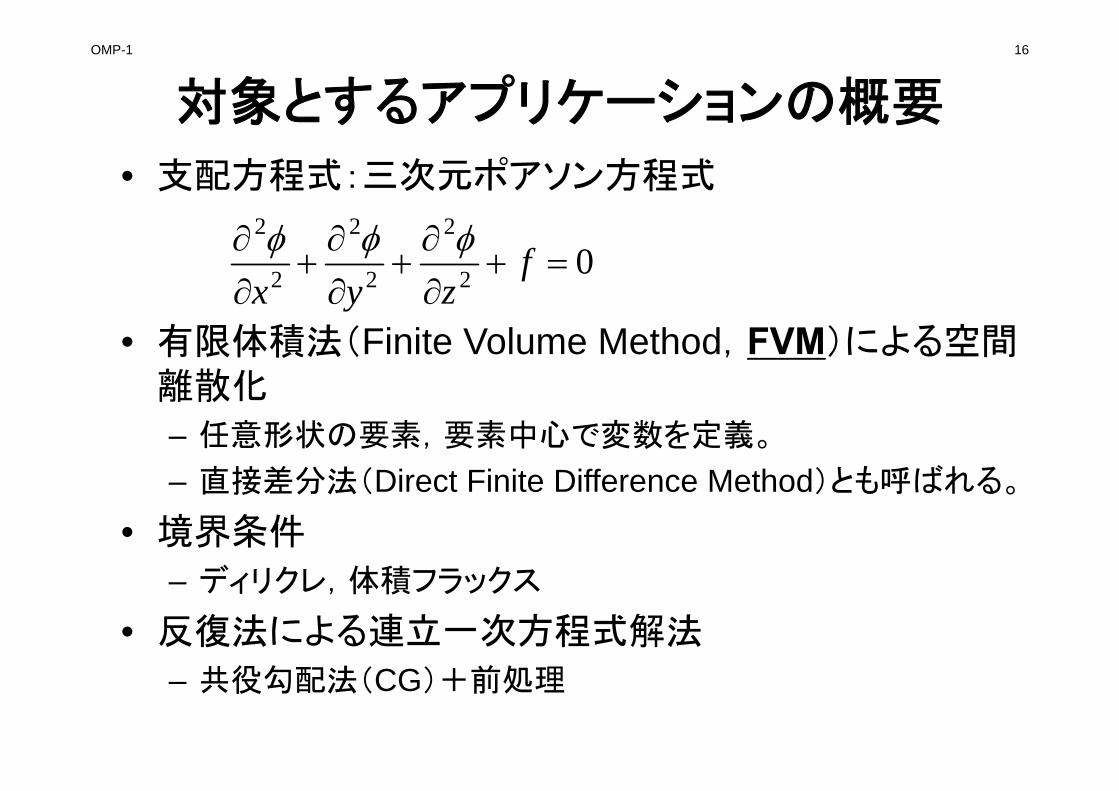
対象とするアプリケーションの概要
• 支配方程式:三次元ポアソン方程式
• 有限体積法(Finite Volume Method,FVM)による空間離散化
– 任意形状の要素,要素中心で変数を定義。
– 直接差分法(Direct Finite Difference Method)とも呼ばれる。
• 境界条件
– ディリクレ,体積フラックス
• 反復法による連立一次方程式解法
– 共役勾配法(CG)+前処理
02
2
2
2
2
2
f
zyx
OMP-1 17
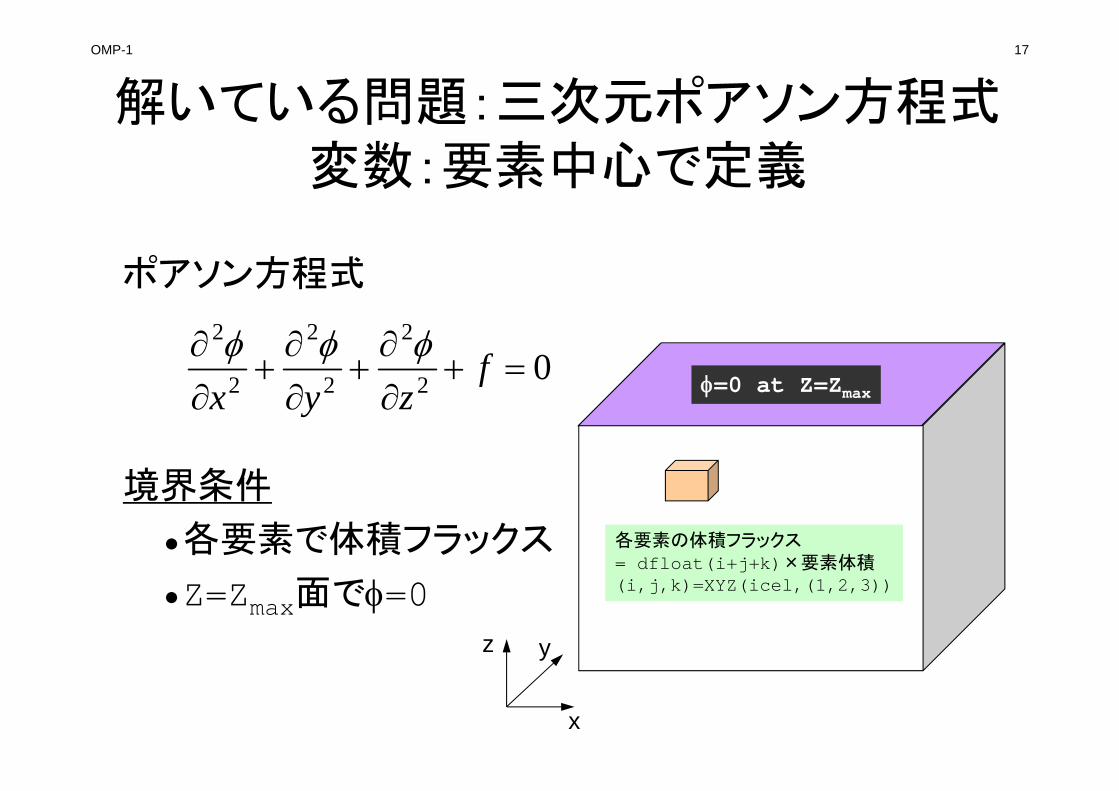
解いている問題:三次元ポアソン方程式変数:要素中心で定義
x
yz
ポアソン方程式
境界条件
•各要素で体積フラックス
•Z=Zmax面で=0
各要素の体積フラックス= dfloat(i+j+k)×要素体積(i,j,k)=XYZ(icel,(1,2,3))
=0 at Z=Zmax02
2
2
2
2
2
f
zyx
OMP-1 18
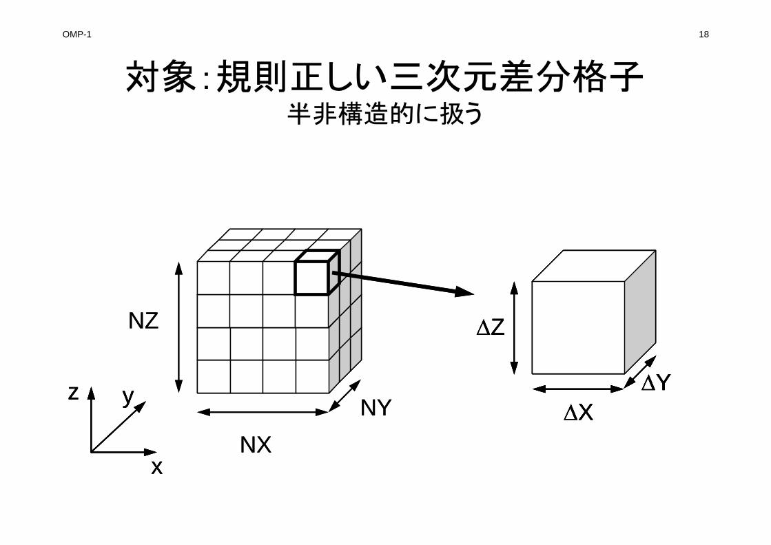
対象:規則正しい三次元差分格子半非構造的に扱う
x
yz
NXNY
NZ Z
XY
x
yz
x
yz
NXNY
NZ Z
XY
Z
XY
XY
OMP-1 19
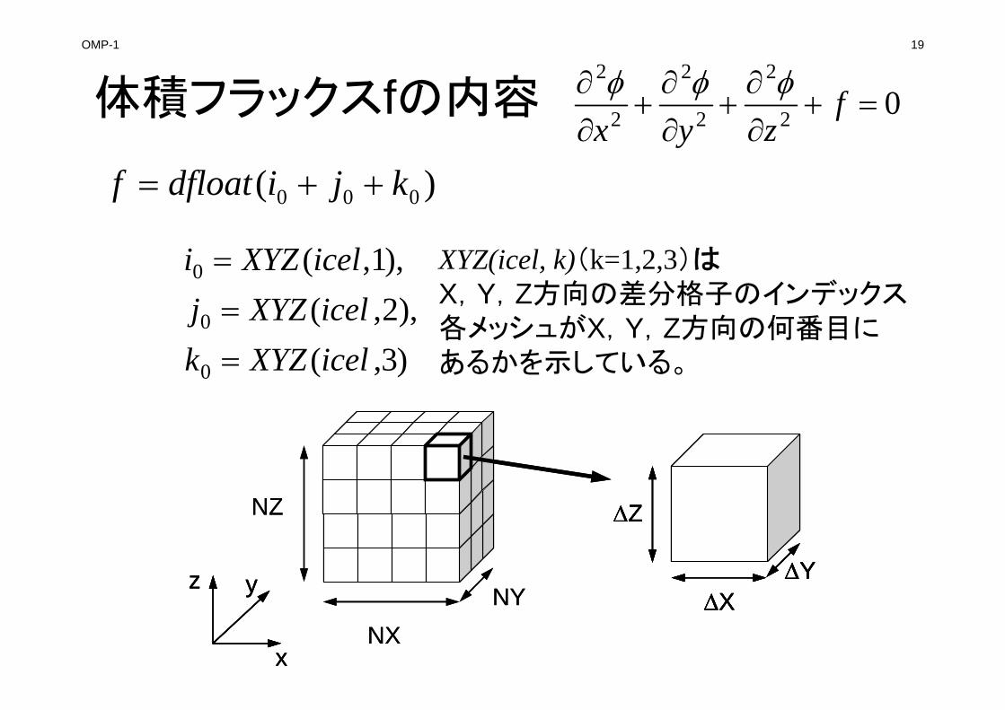
体積フラックスfの内容
x
yz
NXNY
NZ Z
XY
x
yz
x
yz
NXNY
NZ Z
XY
Z
XY
XY
)( 000 kjidfloatf
)3,(),2,(
),1,(
0
0
0
icelXYZkicelXYZjicelXYZi
XYZ(icel, k)(k=1,2,3)は
X,Y,Z方向の差分格子のインデックス各メッシュがX,Y,Z方向の何番目にあるかを示している。
02
2
2
2
2
2
f
zyx
OMP-1 20
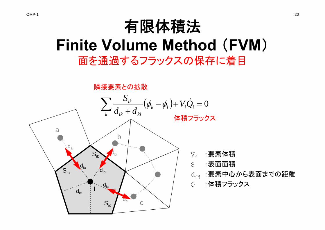
有限体積法Finite Volume Method (FVM)
面を通過するフラックスの保存に着目
i
Sia
Sib
Sic
dia dib
dic
ab
c
dbi
dai
dci
0 ii
kik
kiik
ik QVdd
S
Vi :要素体積
S :表面面積
dij :要素中心から表面までの距離
Q :体積フラックス
隣接要素との拡散
体積フラックス
die
OMP-1 21
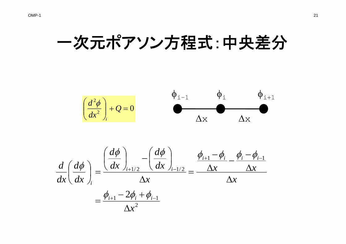
一次元ポアソン方程式:中央差分
211
11
2/12/1
2x
xxx
xdxd
dxd
dxd
dxd
iii
iiii
ii
i
02
2
Q
dxd
i
x x
i-1 i i+1

OMP-1 22
有限体積法Finite Volume Method (FVM)
面を通過するフラックスの保存に着目
i
Sia
Sib
Sic
dia dib
dic
ab
c
dbi
dai
dci
0 ii
kik
kiik
ik QVdd
S
Vi :要素体積
S :表面面積
dij :要素中心から表面までの距離
Q :体積フラックス
隣接要素との拡散
体積フラックス
die
OMP-1 23
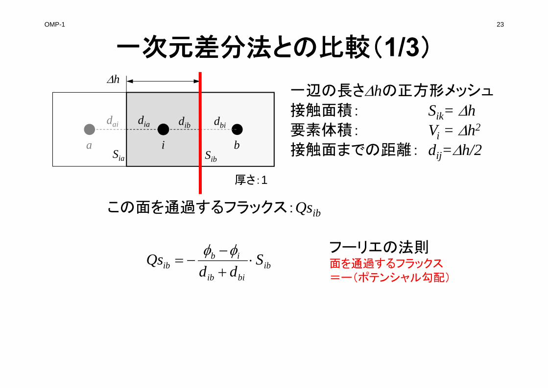
一次元差分法との比較(1/3)
ibbiib
ibib S
ddQs
iSia Sib
dia dib dbi
a b
dai
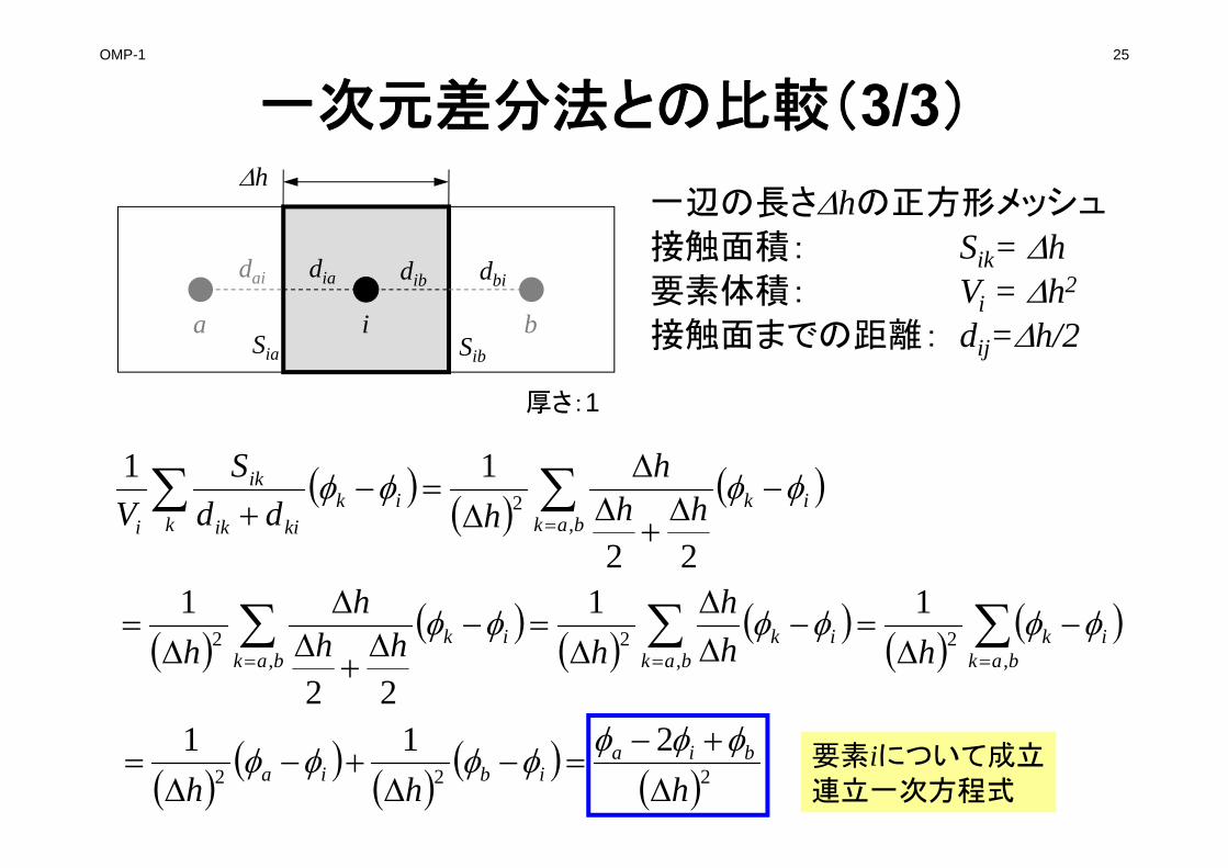
一辺の長さhの正方形メッシュ
接触面積: Sik= h要素体積: Vi = h2
接触面までの距離: dij=h/2
h
この面を通過するフラックス:Qsib
フーリエの法則面を通過するフラックス=ー(ポテンシャル勾配)
厚さ:1
OMP-1 24
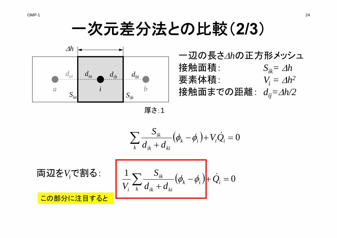
一次元差分法との比較(2/3)
0 ii
kik
kiik
ik QVdd
S
01
ik
ikkiik
ik
i
Qdd
SV
両辺をViで割る:
この部分に注目すると
iSia Sib
dia dib dbi
a b
dai
h一辺の長さhの正方形メッシュ
接触面積: Sik= h要素体積: Vi = h2
接触面までの距離: dij=h/2
厚さ:1
OMP-1 25
一次元差分法との比較(3/3)
222211hhh
biaibia
iSia Sib
dia dib dbi
a b
dai
bakik
kik
kiik
ik
ihh
hhdd
SV ,
2
22
11
h
bakik
bakik
bakik hh
hhhh
hh ,
2,
2,
211
22
1
一辺の長さhの正方形メッシュ
接触面積: Sik= h要素体積: Vi = h2
接触面までの距離: dij=h/2
厚さ:1
要素iについて成立連立一次方程式
OMP-1 26
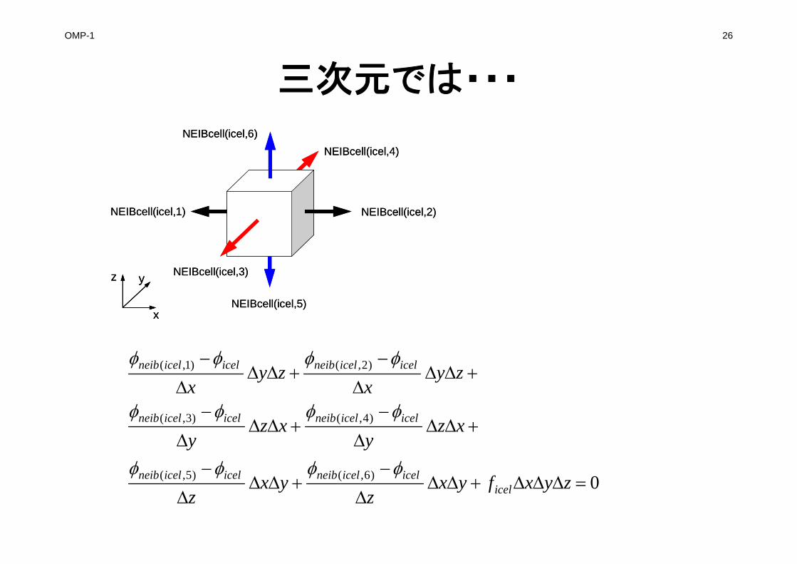
三次元では・・・
NEIBcell(icel,2)NEIBcell(icel,1)
NEIBcell(icel,3)
NEIBcell(icel,5)
NEIBcell(icel,4)NEIBcell(icel,6)
NEIBcell(icel,2)NEIBcell(icel,1)
NEIBcell(icel,3)
NEIBcell(icel,5)
NEIBcell(icel,4)NEIBcell(icel,6)
x
yz
x
yz
0
)6,()5,(
)4,()3,(
)2,()1,(
zyxfyxz
yxz
xzy
xzy
zyx
zyx
icelicelicelneibicelicelneib
icelicelneibicelicelneib
icelicelneibicelicelneib
OMP-1 27
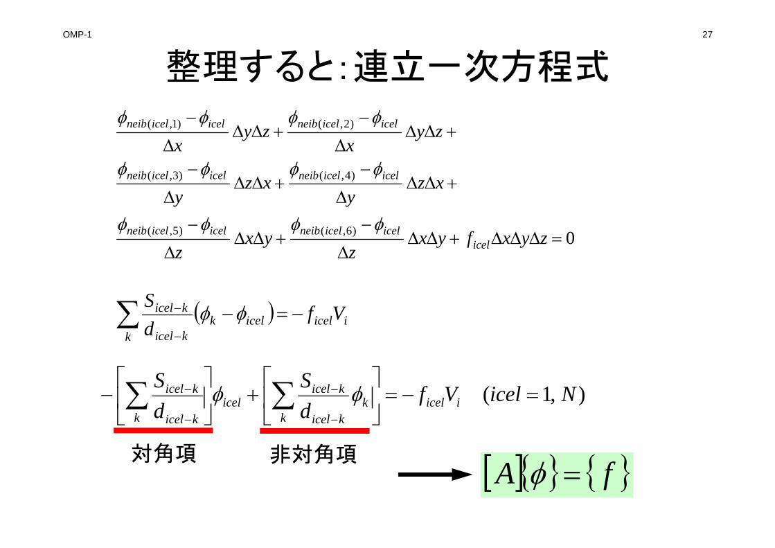
整理すると:連立一次方程式
iicelk
icelkkicel
kicel VfdS
0
)6,()5,(
)4,()3,(
)2,()1,(
zyxfyxz
yxz
xzy
xzy
zyx
zyx
icelicelicelneibicelicelneib
icelicelneibicelicelneib
icelicelneibicelicelneib
fA 対角項 非対角項
),1( NicelVfdS
dS
iicelk
kkicel
kicelicel
k kicel
kicel
28
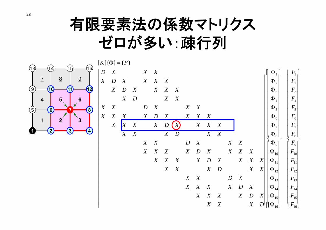
有限要素法の係数マトリクスゼロが多い:疎行列
16
15
14
13
12
11
10
9
8
7
6
5
4
3
2
1
16
15
14
13
12
11
10
9
8
7
6
5
4
3
2
1
}{}]{[
FFFFFFFFFFFFFFFF
DXXXXDXXXX
XDXXXXXDXX
XXDXXXXXXXDXXXX
XXXXDXXXXXXXDXX
XXDXXXXXXXDXXXX
XXXXDXXXXXXXDXX
XXDXXXXXDX
XXXXDXXXXD
FK
1
1
2 3
4 5 6
7 8 9
2 3 4
5 6 7 8
9 10 11 12
13 14 15 16
OMP-1 29
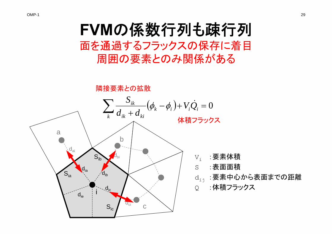
FVMの係数行列も疎行列面を通過するフラックスの保存に着目
周囲の要素とのみ関係がある
i
Sia
Sib
Sic
dia dib
dic
ab
c
dbi
dai
dci
0 ii
kik
kiik
ik QVdd
S
Vi :要素体積
S :表面面積
dij :要素中心から表面までの距離
Q :体積フラックス
隣接要素との拡散
体積フラックス
die
1D-Part1
30
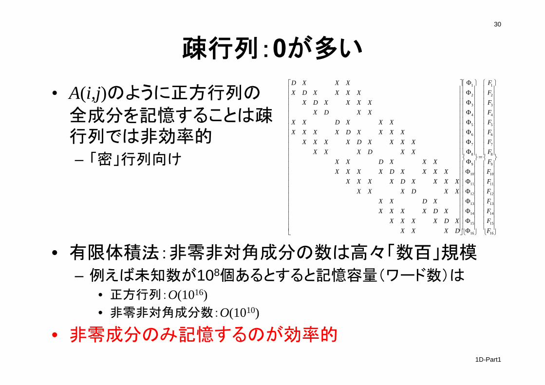
疎行列:0が多い
• A(i,j)のように正方行列の
全成分を記憶することは疎行列では非効率的– 「密」行列向け
16
15
14
13
12
11
10
9
8
7
6
5
4
3
2
1
16
15
14
13
12
11
10
9
8
7
6
5
4
3
2
1
FFFFFFFFFFFFFFFF
DXXXXDXXXX
XDXXXXXDXX
XXDXXXXXXXDXXXX
XXXXDXXXXXXXDXX
XXDXXXXXXXDXXXX
XXXXDXXXXXXXDXX
XXDXXXXXDX
XXXXDXXXXD
• 有限体積法:非零非対角成分の数は高々「数百」規模– 例えば未知数が108個あるとすると記憶容量(ワード数)は
• 正方行列:O(1016)• 非零非対角成分数:O(1010)
• 非零成分のみ記憶するのが効率的
1D-Part1
31
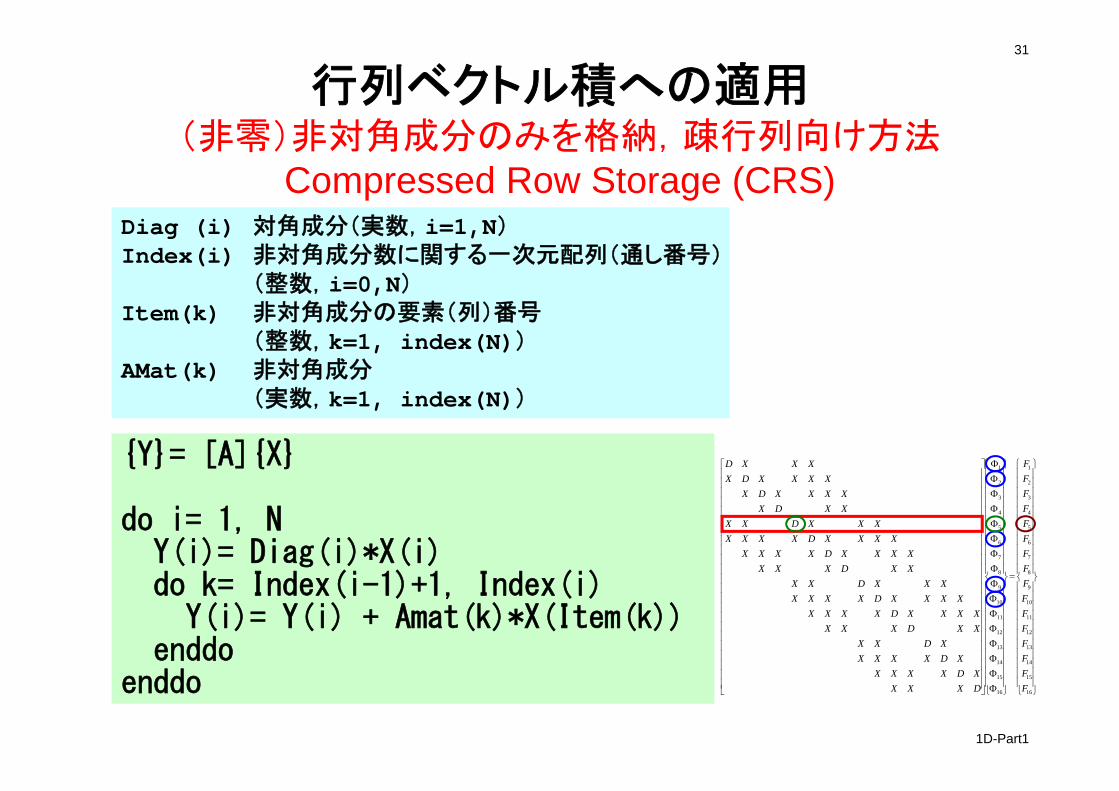
行列ベクトル積への適用(非零)非対角成分のみを格納,疎行列向け方法
Compressed Row Storage (CRS)Diag (i) 対角成分(実数,i=1,N)Index(i) 非対角成分数に関する一次元配列(通し番号)
(整数,i=0,N)Item(k) 非対角成分の要素(列)番号
(整数,k=1, index(N))AMat(k) 非対角成分
(実数,k=1, index(N))
{Y}= [A]{X}
do i= 1, NY(i)= Diag(i)*X(i)do k= Index(i-1)+1, Index(i)
Y(i)= Y(i) + Amat(k)*X(Item(k))enddo
enddo
16
15
14
13
12
11
10
9
8
7
6
5
4
3
2
1
16
15
14
13
12
11
10
9
8
7
6
5
4
3
2
1
FFFFFFFFFFFFFFFF
DXXXXDXXXX
XDXXXXXDXX
XXDXXXXXXXDXXXX
XXXXDXXXXXXXDXX
XXDXXXXXXXDXXXX
XXXXDXXXXXXXDXX
XXDXXXXXDX
XXXXDXXXXD
1D-Part1
32
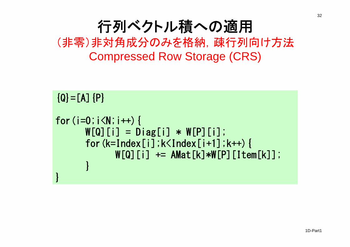
行列ベクトル積への適用(非零)非対角成分のみを格納,疎行列向け方法
Compressed Row Storage (CRS)
{Q}=[A]{P}
for(i=0;i<N;i++){W[Q][i] = Diag[i] * W[P][i]; for(k=Index[i];k<Index[i+1];k++){
W[Q][i] += AMat[k]*W[P][Item[k]];}
}
1D-Part1
33
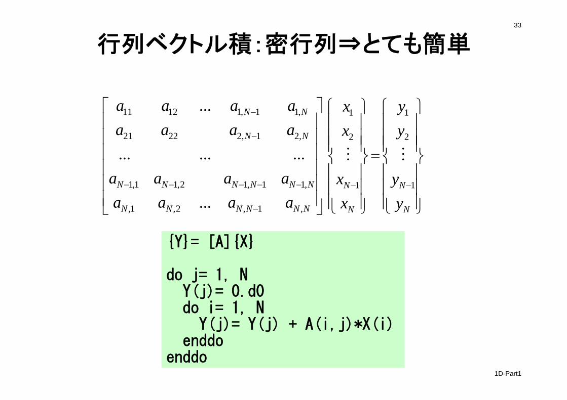
行列ベクトル積:密行列⇒とても簡単
NNNNNN
NNNNNN
NN
NN
aaaaaaaa
aaaaaaaa
,1,2,1,
,11,12,11,1
,21,22221
,11,11211
...
.........
...
N
N
N
N
yy
yy
xx
xx
1
2
1
1
2
1
{Y}= [A]{X}
do j= 1, NY(j)= 0.d0do i= 1, N
Y(j)= Y(j) + A(i,j)*X(i)enddo
enddo
34
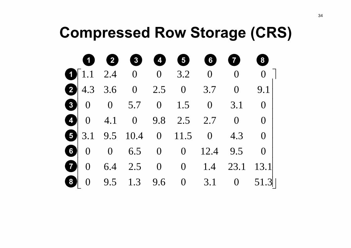
Compressed Row Storage (CRS)
3.5101.306.93.15.901.131.234.1005.24.60
05.94.12005.60003.405.1104.105.91.3007.25.28.901.4001.305.107.5001.907.305.206.33.4
0002.3004.21.11
2
3
4
5
6
7
8
1 2 3 4 5 6 7 8
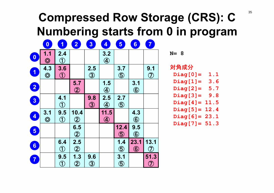
35Compressed Row Storage (CRS): CNumbering starts from 0 in program
2.4①
3.2④
4.3◎
2.5③
3.7⑤
9.1⑦
1.5④
3.1⑥
4.1①
2.5④
2.7⑤
3.1◎
9.5①
10.4②
4.3⑥
6.5②
9.5⑥
6.4①
2.5②
1.4⑤
13.1⑦
9.5①
1.3②
9.6③
3.1⑤
N= 8
対角成分Diag[0]= 1.1 Diag[1]= 3.6Diag[2]= 5.7Diag[3]= 9.8 Diag[4]= 11.5 Diag[5]= 12.4Diag[6]= 23.1 Diag[7]= 51.3
1.1◎
3.6①
5.7②
9.8③
11.5④
12.4⑤
23.1⑥
51.3⑦
0 1 2 3 4 5 6 7
0
1
2
3
4
5
6
7
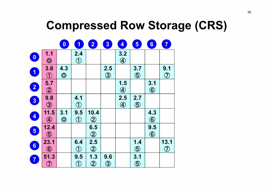
36
Compressed Row Storage (CRS)0
2.4①
3.2④
4.3◎
2.5③
3.7⑤
9.1⑦
1.5④
3.1⑥
4.1①
2.5④
2.7⑤
3.1◎
9.5①
10.4②
4.3⑥
6.5②
9.5⑥
6.4①
2.5②
1.4⑤
13.1⑦
9.5①
1.3②
9.6③
3.1⑤
1 2 3 4 5 6 71.1◎
3.6①
5.7②
9.8③
11.5④
12.4⑤
23.1⑥
51.3⑦
0
1
2
3
4
5
6
7
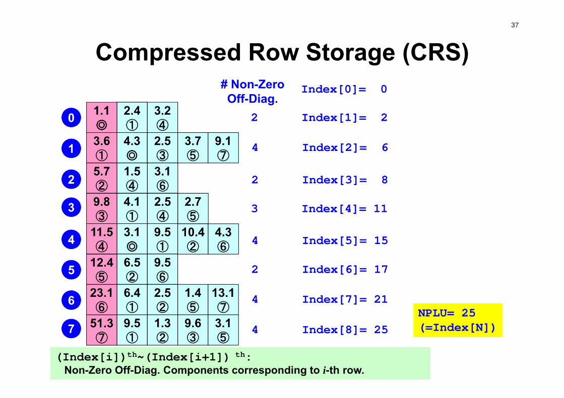
37
Compressed Row Storage (CRS)
0
1
2
3
4
5
6
7
2.4①
3.2④
4.3◎
2.5③
3.7⑤
9.1⑦
1.5④
3.1⑥
4.1①
2.5④
2.7⑤
3.1◎
9.5①
10.4②
4.3⑥
6.5②
9.5⑥
6.4①
2.5②
1.4⑤
13.1⑦
9.5①
1.3②
9.6③
3.1⑤
1.1◎
3.6①
5.7②
9.8③
11.5④
12.4⑤
23.1⑥
51.3⑦
# Non-ZeroOff-Diag.
2 Index[1]= 2
4 Index[2]= 6
2 Index[3]= 8
3 Index[4]= 11
4 Index[5]= 15
2 Index[6]= 17
4 Index[7]= 21
4 Index[8]= 25
Index[0]= 0
NPLU= 25(=Index[N])
(Index[i])th~(Index[i+1]) th:Non-Zero Off-Diag. Components corresponding to i-th row.
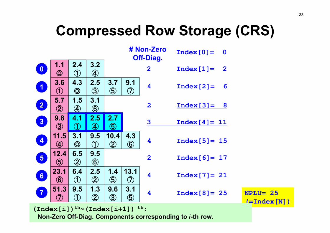
38
Compressed Row Storage (CRS)
0
1
2
3
4
5
6
7
2.4①
3.2④
4.3◎
2.5③
3.7⑤
9.1⑦
1.5④
3.1⑥
3.1◎
9.5①
10.4②
4.3⑥
6.5②
9.5⑥
6.4①
2.5②
1.4⑤
13.1⑦
9.5①
1.3②
9.6③
3.1⑤
1.1◎
3.6①
5.7②
9.8③
11.5④
12.4⑤
23.1⑥
51.3⑦
4.1①
2.5④
2.7⑤
NPLU= 25(=Index[N])
2 Index[1]= 2
4 Index[2]= 6
2 Index[3]= 8
3 Index[4]= 11
4 Index[5]= 15
2 Index[6]= 17
4 Index[7]= 21
4 Index[8]= 25
Index[0]= 0# Non-ZeroOff-Diag.
(Index[i])th~(Index[i+1]) th:Non-Zero Off-Diag. Components corresponding to i-th row.
39
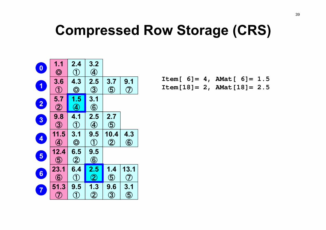
Compressed Row Storage (CRS)
Item[ 6]= 4, AMat[ 6]= 1.5Item[18]= 2, AMat[18]= 2.5
0
1
2
3
4
5
6
7
2.4①
3.2④
4.3◎
2.5③
3.7⑤
9.1⑦
3.1⑥
4.1①
2.5④
2.7⑤
3.1◎
9.5①
10.4②
4.3⑥
6.5②
9.5⑥
6.4①
1.4⑤
13.1⑦
9.5①
1.3②
9.6③
3.1⑤
1.1◎
3.6①
5.7②
9.8③
11.5④
12.4⑤
23.1⑥
51.3⑦
1.5④
2.5②
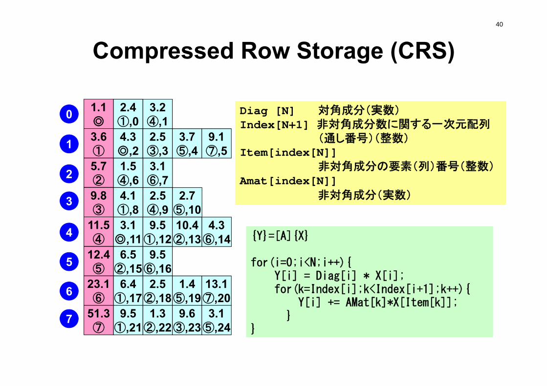
Compressed Row Storage (CRS)40
0
1
2
3
4
5
6
7
2.4①,0
3.2④,1
4.3◎,2
2.5③,3
3.7⑤,4
9.1⑦,5
1.5④,6
3.1⑥,7
4.1①,8
2.5④,9
2.7⑤,10
3.1◎,11
9.5①,12
10.4②,13
4.3⑥,14
6.5②,15
9.5⑥,16
6.4①,17
2.5②,18
1.4⑤,19
13.1⑦,20
9.5①,21
1.3②,22
9.6③,23
3.1⑤,24
1.1◎
3.6①
5.7②
9.8③
11.5④
12.4⑤
23.1⑥
51.3⑦
{Y}=[A]{X}
for(i=0;i<N;i++){Y[i] = Diag[i] * X[i]; for(k=Index[i];k<Index[i+1];k++){
Y[i] += AMat[k]*X[Item[k]];}
}
Diag [N] 対角成分(実数)Index[N+1] 非対角成分数に関する一次元配列
(通し番号)(整数)Item[index[N]]
非対角成分の要素(列)番号(整数)Amat[index[N]]
非対角成分(実数)
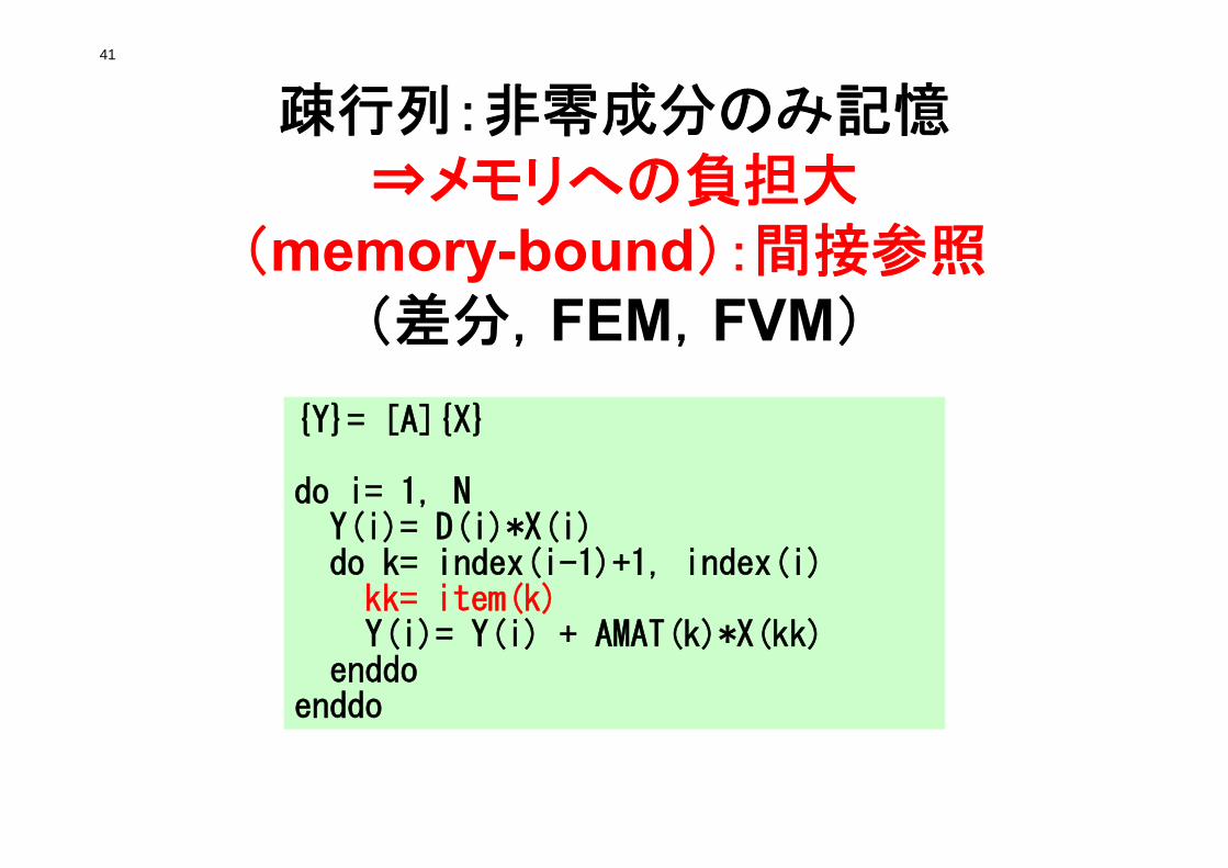
41
疎行列:非零成分のみ記憶⇒メモリへの負担大
(memory-bound):間接参照(差分,FEM,FVM)
{Y}= [A]{X}
do i= 1, NY(i)= D(i)*X(i)do k= index(i-1)+1, index(i)kk= item(k)Y(i)= Y(i) + AMAT(k)*X(kk)
enddoenddo
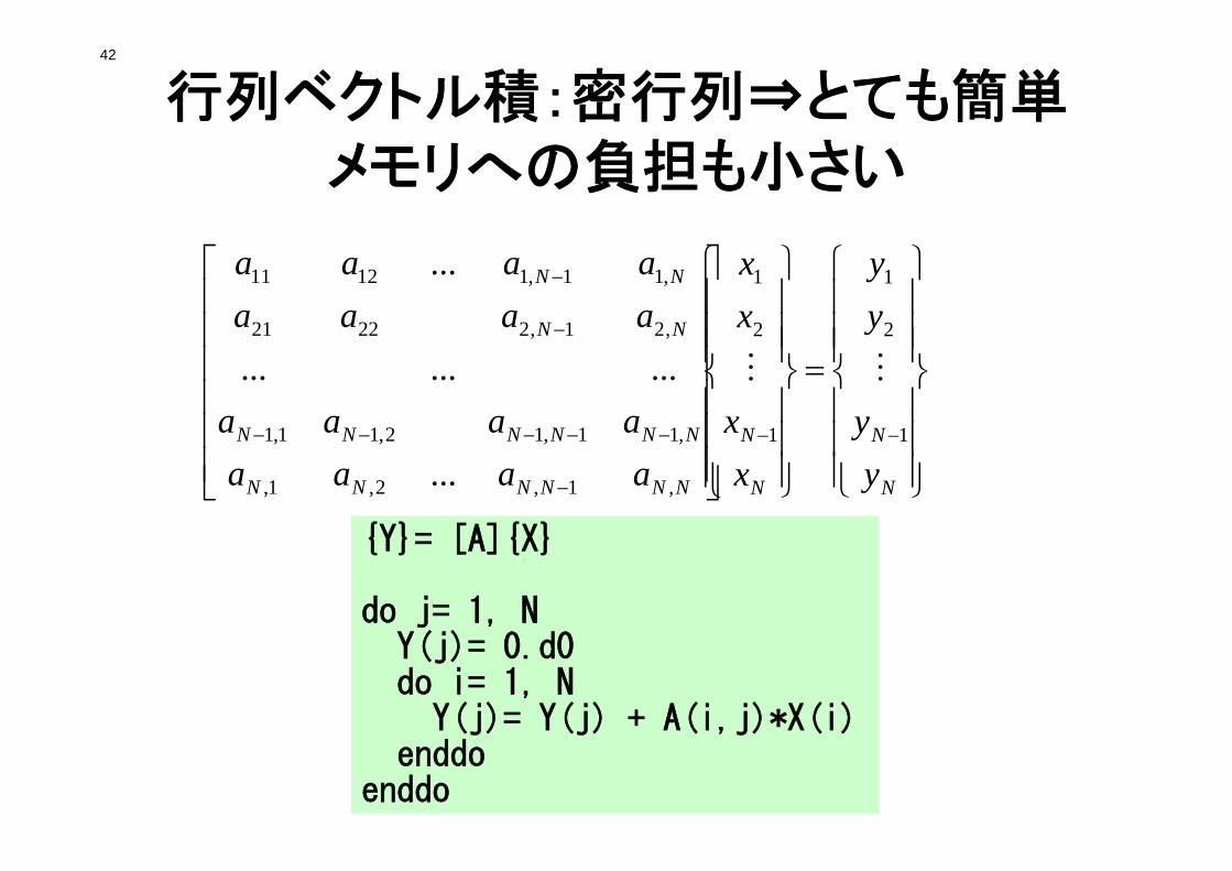
42
行列ベクトル積:密行列⇒とても簡単メモリへの負担も小さい
NNNNNN
NNNNNN
NN
NN
aaaaaaaa
aaaaaaaa
,1,2,1,
,11,12,11,1
,21,22221
,11,11211
...
.........
...
N
N
N
N
yy
yy
xx
xx
1
2
1
1
2
1
{Y}= [A]{X}
do j= 1, NY(j)= 0.d0do i= 1, N
Y(j)= Y(j) + A(i,j)*X(i)enddo
enddo
43
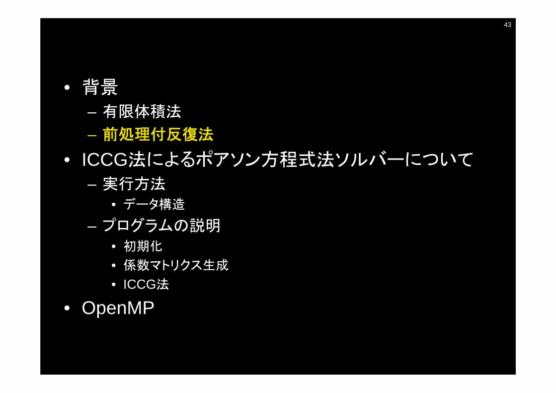
• 背景
– 有限体積法
– 前処理付反復法
• ICCG法によるポアソン方程式法ソルバーについて
– 実行方法• データ構造
– プログラムの説明• 初期化
• 係数マトリクス生成
• ICCG法
• OpenMP
44
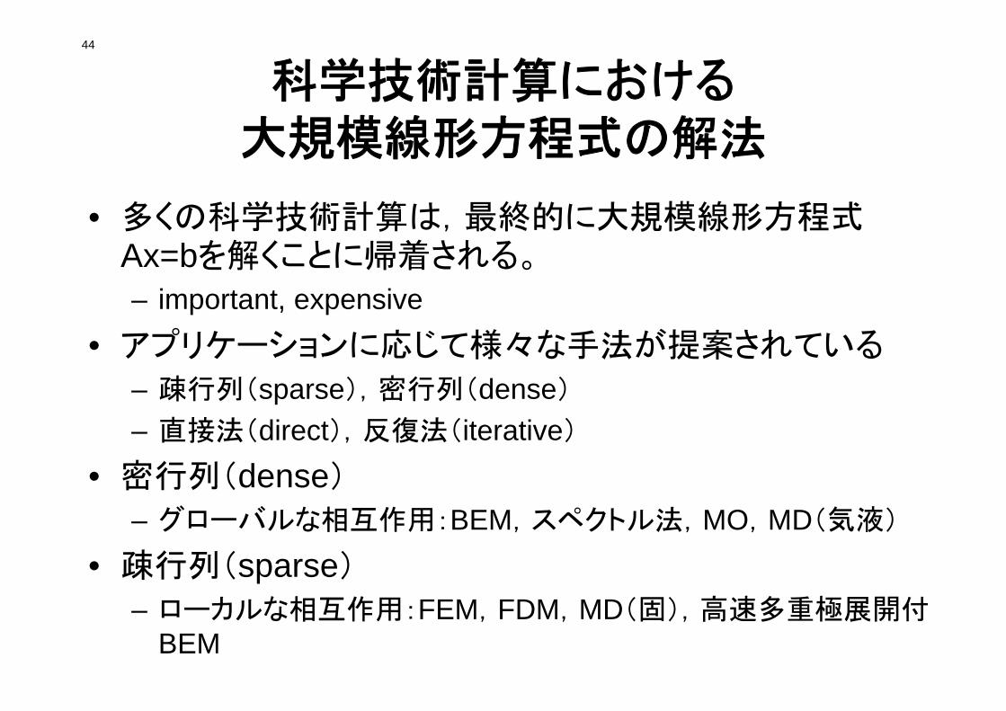
科学技術計算における大規模線形方程式の解法
• 多くの科学技術計算は, 終的に大規模線形方程式Ax=bを解くことに帰着される。
– important, expensive• アプリケーションに応じて様々な手法が提案されている
– 疎行列(sparse),密行列(dense)
– 直接法(direct),反復法(iterative)
• 密行列(dense)
– グローバルな相互作用:BEM,スペクトル法,MO,MD(気液)
• 疎行列(sparse)
– ローカルな相互作用:FEM,FDM,MD(固),高速多重極展開付BEM
45
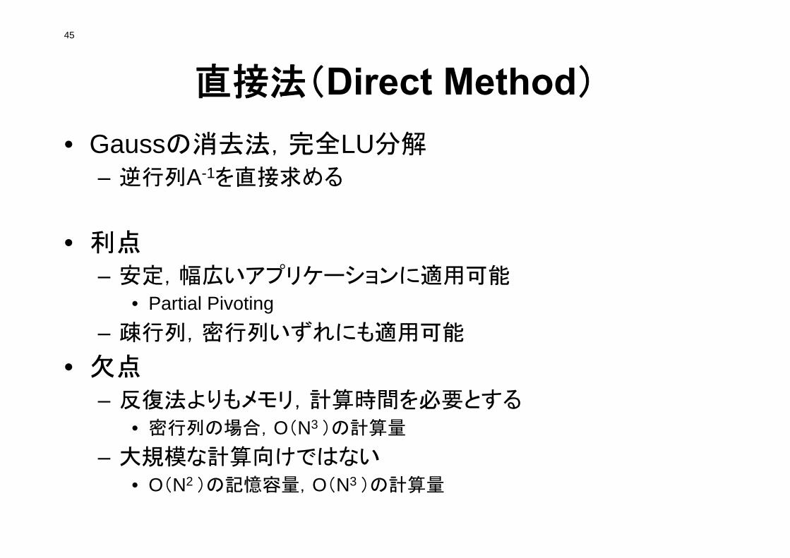
直接法(Direct Method)
• Gaussの消去法,完全LU分解– 逆行列A-1を直接求める
• 利点– 安定,幅広いアプリケーションに適用可能
• Partial Pivoting– 疎行列,密行列いずれにも適用可能
• 欠点– 反復法よりもメモリ,計算時間を必要とする
• 密行列の場合,O(N3 )の計算量
– 大規模な計算向けではない• O(N2 )の記憶容量,O(N3 )の計算量
46
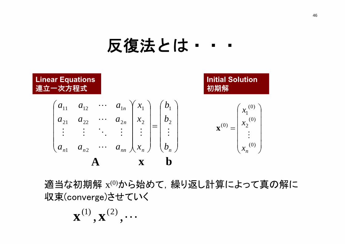
反復法とは・・・
適当な初期解 x(0)から始めて,繰り返し計算によって真の解に
収束(converge)させていく
,, )2()1( xx
A b
Initial Solution初期解
Linear Equations連立一次方程式
)0(
)0(2
)0(1
)0(
nx
xx
x
x
nnnnnn
n
n
b
bb
x
xx
aaa
aaaaaa
2
1
2
1
21
22221
11211
47
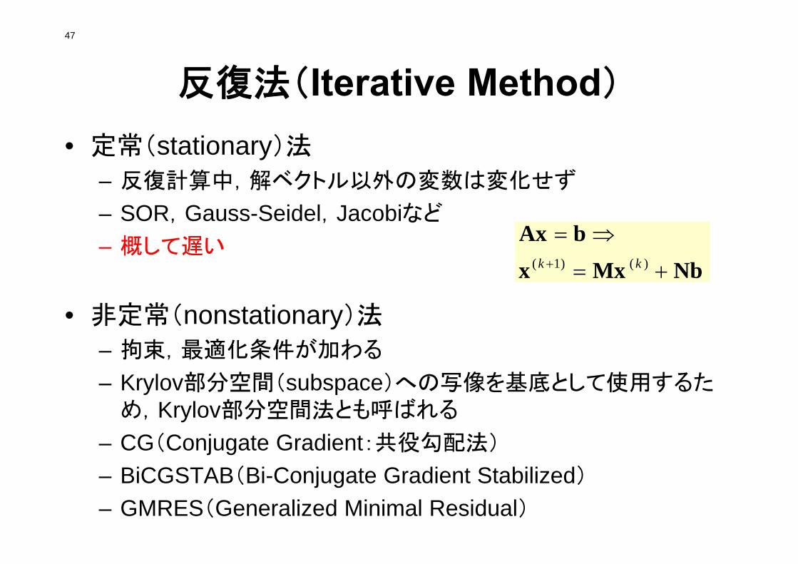
反復法(Iterative Method)
• 定常(stationary)法
– 反復計算中,解ベクトル以外の変数は変化せず
– SOR,Gauss-Seidel,Jacobiなど
– 概して遅い
• 非定常(nonstationary)法
– 拘束, 適化条件が加わる
– Krylov部分空間(subspace)への写像を基底として使用するため,Krylov部分空間法とも呼ばれる
– CG(Conjugate Gradient:共役勾配法)
– BiCGSTAB(Bi-Conjugate Gradient Stabilized)
– GMRES(Generalized Minimal Residual)
NbMxxbAx
)()1( kk
48
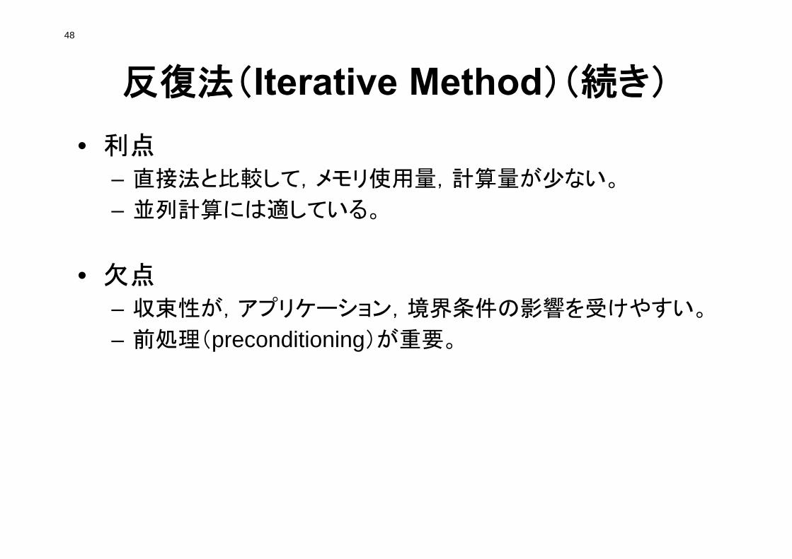
反復法(Iterative Method)(続き)
• 利点– 直接法と比較して,メモリ使用量,計算量が少ない。
– 並列計算には適している。
• 欠点– 収束性が,アプリケーション,境界条件の影響を受けやすい。
– 前処理(preconditioning)が重要。
Solver-Iterative49
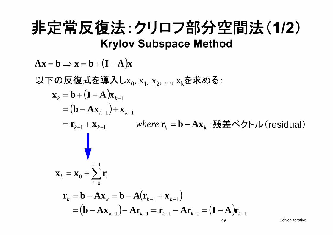
非定常反復法:クリロフ部分空間法(1/2)Krylov Subspace Method xAIbxbAx
以下の反復式を導入しx0, x1, x2, ..., xkを求める:
11
11
1
kk
kk
kk
xrxAxb
xAIbx
kkwhere Axbr :残差ベクトル(residual)
1
00
k
iik rxx
11111
11
kkkkk
kkkk
rAIArrArAxbxrAbAxbr
Solver-Iterative50
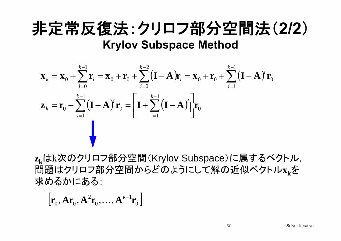
非定常反復法:クリロフ部分空間法(2/2)Krylov Subspace Method
zkはk次のクリロフ部分空間(Krylov Subspace)に属するベクトル,問題はクリロフ部分空間からどのようにして解の近似ベクトルxkを求めるかにある:
0
1
1
1
100
1
1000
2
000
1
00
rAIIrAIrz
rAIrxrAIrxrxx
k
i
ik
i
ik
k
i
ik
ii
k
iik
01
02
00 ,,,, rArAArr k
Solver-Iterative
51
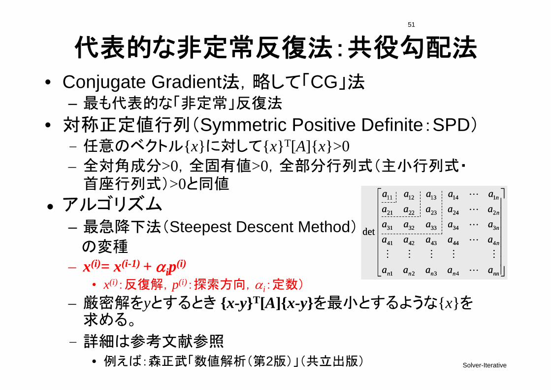
代表的な非定常反復法:共役勾配法• Conjugate Gradient法,略して「CG」法
– も代表的な「非定常」反復法
• 対称正定値行列(Symmetric Positive Definite:SPD)– 任意のベクトル{x}に対して{x}T[A]{x}>0– 全対角成分>0,全固有値>0,全部分行列式(主小行列式・
首座行列式)>0と同値
• アルゴリズム– 急降下法(Steepest Descent Method)
の変種
– x(i)= x(i-1) + ip(i)
• x(i):反復解,p(i):探索方向,i:定数)
– 厳密解をyとするとき {x-y}T[A]{x-y}を 小とするような{x}を求める。
– 詳細は参考文献参照• 例えば:森正武「数値解析(第2版)」(共立出版)
nnnnnn
n
n
n
n
aaaaa
aaaaaaaaaaaaaaaaaaaa
4321
444434241
334333231
224232221
114131211
det
nnnnnn
n
n
n
n
aaaaa
aaaaaaaaaaaaaaaaaaaa
4321
444434241
334333231
224232221
114131211
det
Solver-Iterative
52
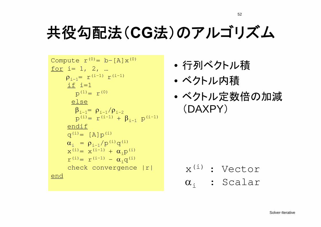
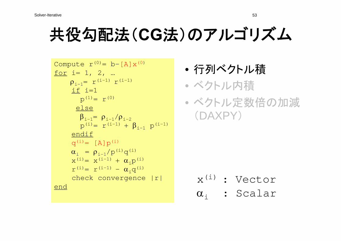
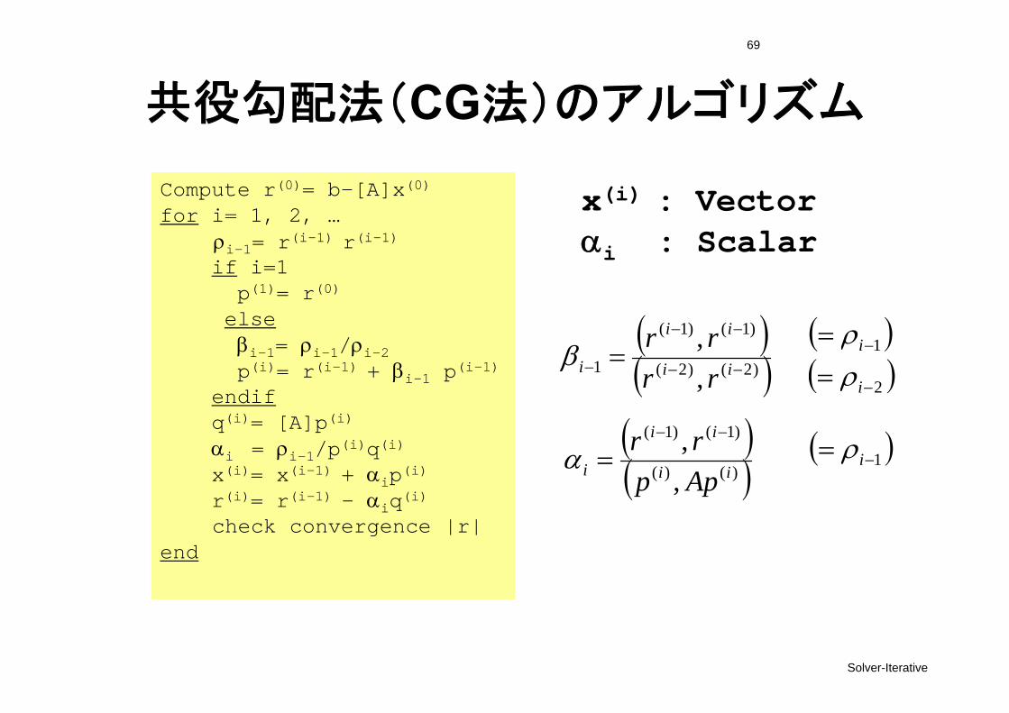
共役勾配法(CG法)のアルゴリズム
Compute r(0)= b-[A]x(0)
for i= 1, 2, …i-1= r(i-1) r(i-1)if i=1p(1)= r(0)
elsei-1= i-1/i-2p(i)= r(i-1) + i-1 p(i-1)
endifq(i)= [A]p(i)
i = i-1/p(i)q(i)x(i)= x(i-1) + ip(i)r(i)= r(i-1) - iq(i)check convergence |r|
end
• 行列ベクトル積
• ベクトル内積
• ベクトル定数倍の加減(DAXPY)
x(i) : Vectori : Scalar
53
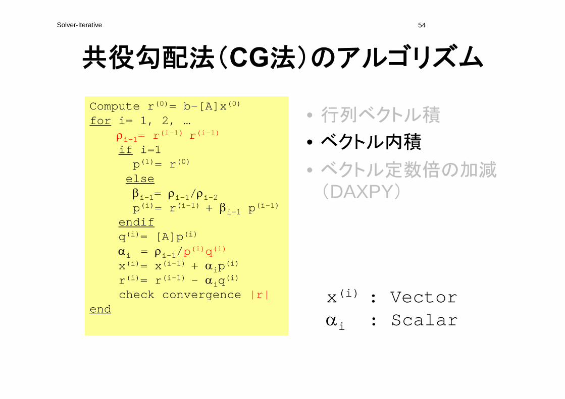
共役勾配法(CG法)のアルゴリズム
Compute r(0)= b-[A]x(0)
for i= 1, 2, …i-1= r(i-1) r(i-1)if i=1p(1)= r(0)
elsei-1= i-1/i-2p(i)= r(i-1) + i-1 p(i-1)
endifq(i)= [A]p(i)
i = i-1/p(i)q(i)x(i)= x(i-1) + ip(i)r(i)= r(i-1) - iq(i)check convergence |r|
end
Solver-Iterative
• 行列ベクトル積
• ベクトル内積
• ベクトル定数倍の加減(DAXPY)
x(i) : Vectori : Scalar
54
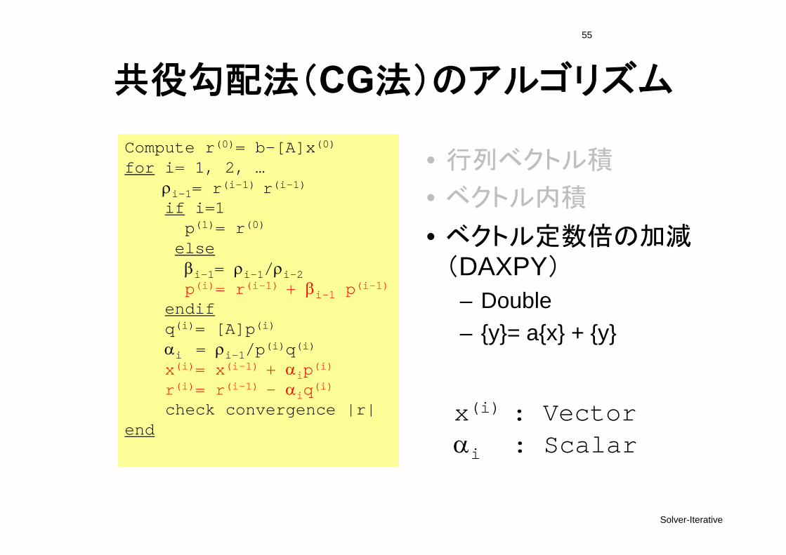
共役勾配法(CG法)のアルゴリズム
Compute r(0)= b-[A]x(0)
for i= 1, 2, …i-1= r(i-1) r(i-1)if i=1p(1)= r(0)
elsei-1= i-1/i-2p(i)= r(i-1) + i-1 p(i-1)
endifq(i)= [A]p(i)
i = i-1/p(i)q(i)x(i)= x(i-1) + ip(i)r(i)= r(i-1) - iq(i)check convergence |r|
end
Solver-Iterative
• 行列ベクトル積
• ベクトル内積
• ベクトル定数倍の加減(DAXPY)
x(i) : Vectori : Scalar
Solver-Iterative
55
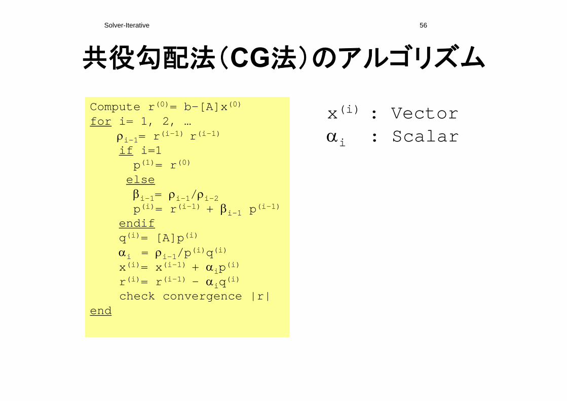
共役勾配法(CG法)のアルゴリズム
x(i) : Vectori : Scalar
Compute r(0)= b-[A]x(0)
for i= 1, 2, …i-1= r(i-1) r(i-1)if i=1p(1)= r(0)
elsei-1= i-1/i-2p(i)= r(i-1) + i-1 p(i-1)
endifq(i)= [A]p(i)
i = i-1/p(i)q(i)x(i)= x(i-1) + ip(i)r(i)= r(i-1) - iq(i)check convergence |r|
end
• 行列ベクトル積
• ベクトル内積
• ベクトル定数倍の加減(DAXPY)
– Double– {y}= a{x} + {y}
Solver-Iterative 56
共役勾配法(CG法)のアルゴリズム
Compute r(0)= b-[A]x(0)
for i= 1, 2, …i-1= r(i-1) r(i-1)if i=1p(1)= r(0)
elsei-1= i-1/i-2p(i)= r(i-1) + i-1 p(i-1)
endifq(i)= [A]p(i)
i = i-1/p(i)q(i)x(i)= x(i-1) + ip(i)r(i)= r(i-1) - iq(i)check convergence |r|
end
x(i) : Vectori : Scalar
57
CG法アルゴリズムの導出(1/5)
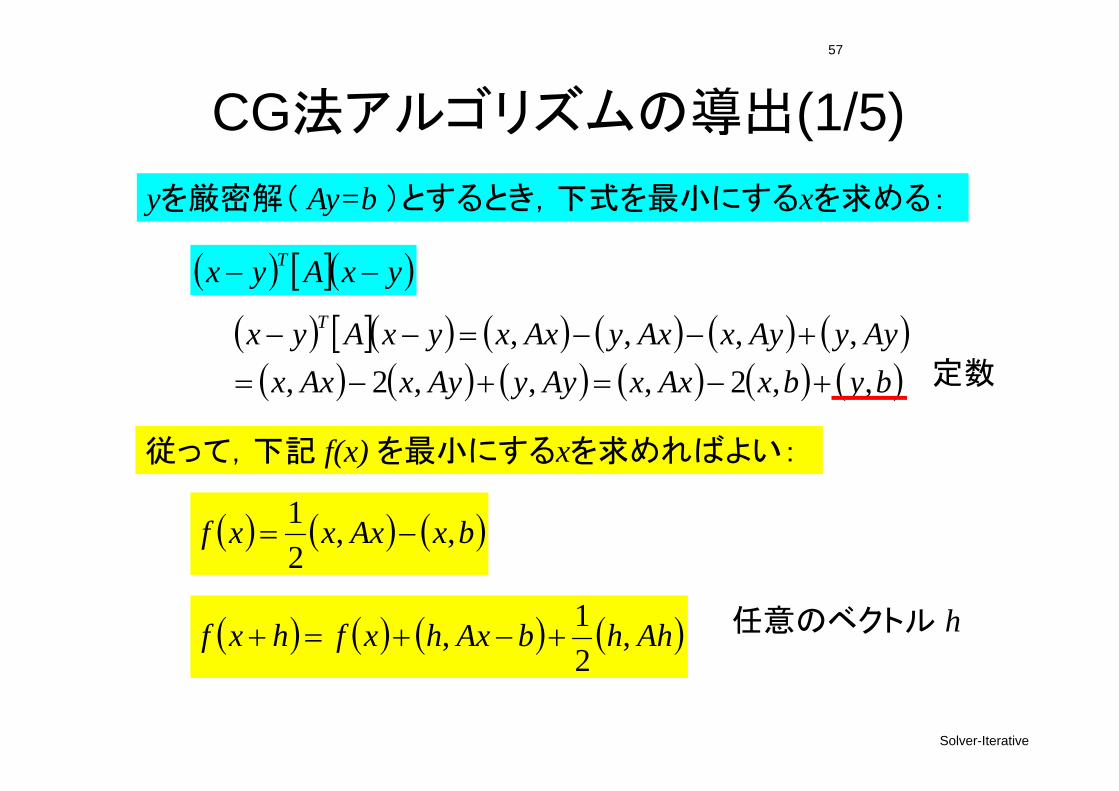
bybxAxxAyyAyxAxx
AyyAyxAxyAxxyxAyx T
,,2,,,2,,,,,
yxAyx T
定数
bxAxxxf ,,21
AhhbAxhxfhxf ,21, 任意のベクトル h
Solver-Iterative
yを厳密解( Ay=b )とするとき,下式を 小にするxを求める:
従って,下記 f(x) を 小にするxを求めればよい:
58
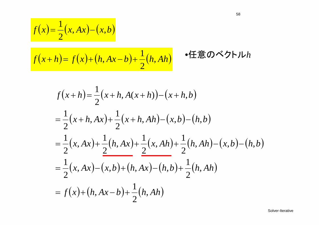
bxAxxxf ,,21
AhhbAxhxfhxf ,21, •任意のベクトルh
AhhbAxhxf
AhhbhAxhbxAxx
bhbxAhhAhxAxhAxx
bhbxAhhxAxhx
bhxhxAhxhxf
,21,
,21,,,,
21
,,,21,
21,
21,
21
,,,21,
21
,)(,21
Solver-Iterative
59
CG法アルゴリズムの導出(2/5)
)()()1( kk
kk pxx
Solver-Iterative
(1)
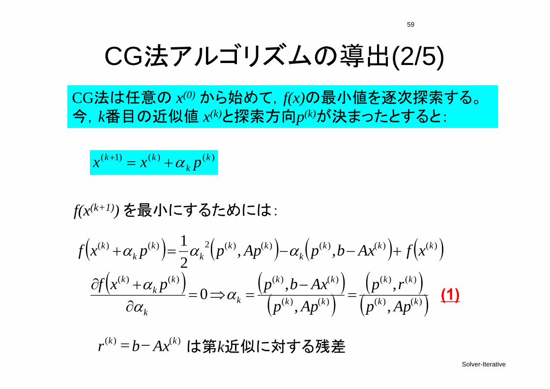
CG法は任意の x(0) から始めて,f(x)の 小値を逐次探索する。今,k番目の近似値 x(k)と探索方向p(k)が決まったとすると:
)()()()()(2)()( ,,21 kkk
kkk
kk
kk xfAxbpApppxf
f(x(k+1)) を 小にするためには:
)()(
)()(
)()(
)()()()(
,,
,,0 kk
kk
kk
kk
kk
kk
k
Apprp
AppAxbppxf
)()( kk Axbr は第k近似に対する残差
60
CG法アルゴリズムの導出(3/5)
)()()1( kk
kk Aprr
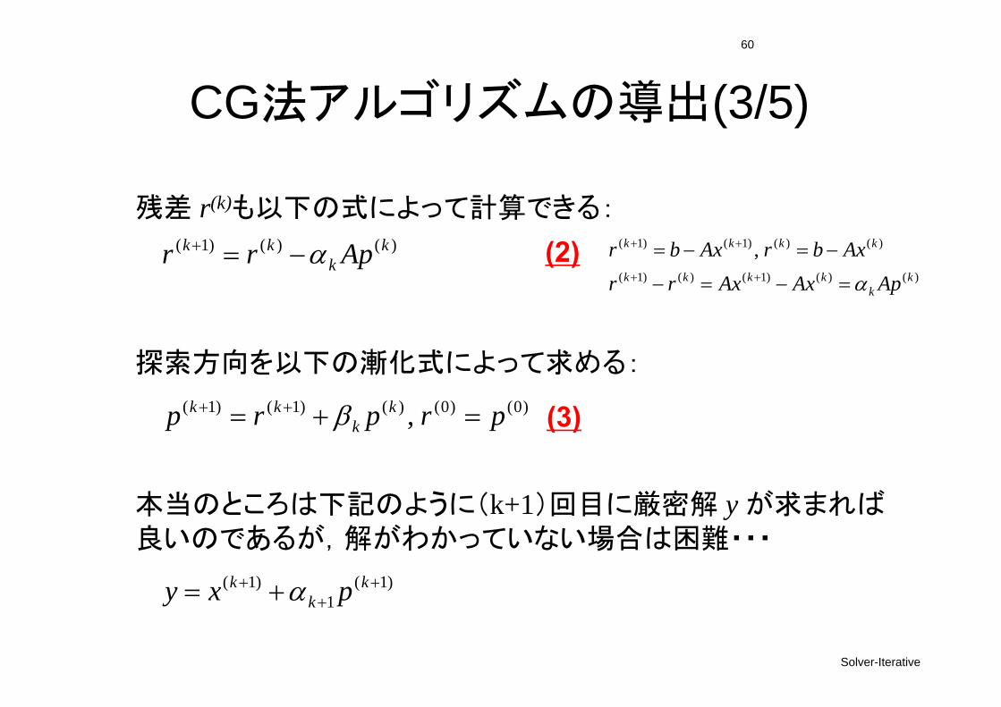
残差 r(k)も以下の式によって計算できる:
本当のところは下記のように(k+1)回目に厳密解 y が求まれば良いのであるが,解がわかっていない場合は困難・・・
)1(1
)1(
kk
k pxy
)()()1()()1(
)()()1()1( ,k
kkkkk
kkkk
ApAxAxrrAxbrAxbr
Solver-Iterative
(2)
)0()0()()1()1( , prprp kk
kk
探索方向を以下の漸化式によって求める:
(3)
61
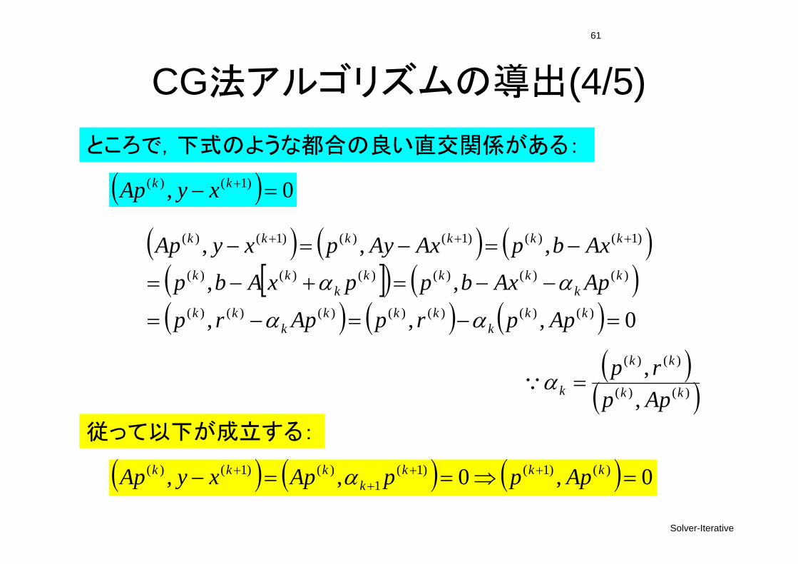
CG法アルゴリズムの導出(4/5)ところで,下式のような都合の良い直交関係がある:
従って以下が成立する:
0,0,, )()1()1(1
)()1()(
kkkk
kkk ApppApxyAp
0,,,
,,,,,
)()()()()()()(
)()()()()()(
)1()()1()()1()(
kkk
kkkk
kk
kk
kkkk
kk
kkkkkk
ApprpAprp
ApAxbppxAbpAxbpAxAypxyAp
)()(
)()(
,,
kk
kk
k Apprp
0, )1()( kk xyAp
Solver-Iterative
62
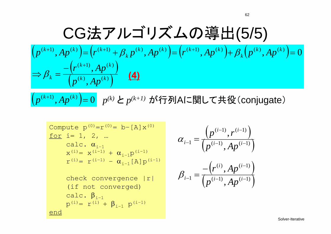
CG法アルゴリズムの導出(5/5)
)()(
)()1(
)()()()1()()()1()()1(
,,
0,,,,
kk
kk
k
kkk
kkkkk
kkk
AppApr
AppAprApprApp
0, )()1( kk App p(k) と p(k+1) が行列Aに関して共役(conjugate)
Solver-Iterative
(4)
)1()1(
)1()(
1 ,,
ii
ii
i AppApr
Compute p(0)=r(0)= b-[A]x(0)
for i= 1, 2, …calc. i-1x(i)= x(i-1) + i-1p(i-1)r(i)= r(i-1) – i-1[A]p(i-1)
check convergence |r|(if not converged)calc. i-1p(i)= r(i) + i-1 p(i-1)
end
)1()1(
)1()1(
1 ,,
ii
ii
i Apprp
63
CG法アルゴリズム
Solver-Iterative
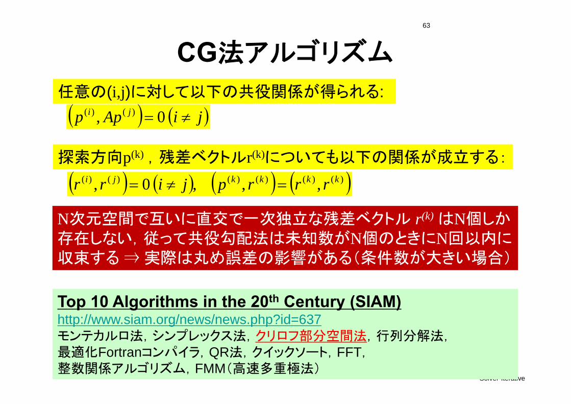
任意の(i,j)に対して以下の共役関係が得られる:
N次元空間で互いに直交で一次独立な残差ベクトル r(k) はN個しか存在しない,従って共役勾配法は未知数がN個のときにN回以内に収束する ⇒ 実際は丸め誤差の影響がある(条件数が大きい場合)
jiApp ji 0, )()(
)()()()()()( ,,,0, kkkkji rrrpjirr
探索方向p(k) ,残差ベクトルr(k)についても以下の関係が成立する:
Top 10 Algorithms in the 20th Century (SIAM)http://www.siam.org/news/news.php?id=637モンテカルロ法,シンプレックス法,クリロフ部分空間法,行列分解法,
適化Fortranコンパイラ,QR法,クイックソート,FFT,整数関係アルゴリズム,FMM(高速多重極法)
64
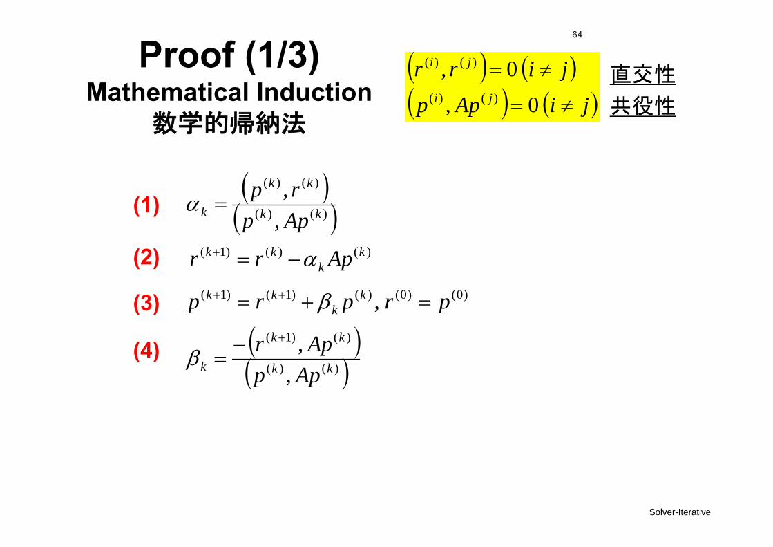
Proof (1/3)Mathematical Induction
数学的帰納法
Solver-Iterative
jiApp
jirrji
ji
0,0,
)()(
)()(
)()(
)()(
,,
kk
kk
k Apprp
(1)
(2)
(3)
(4)
)()()1( kk
kk Aprr
)0()0()()1()1( , prprp kk
kk
)()(
)()1(
,,
kk
kk
k AppApr
直交性
共役性
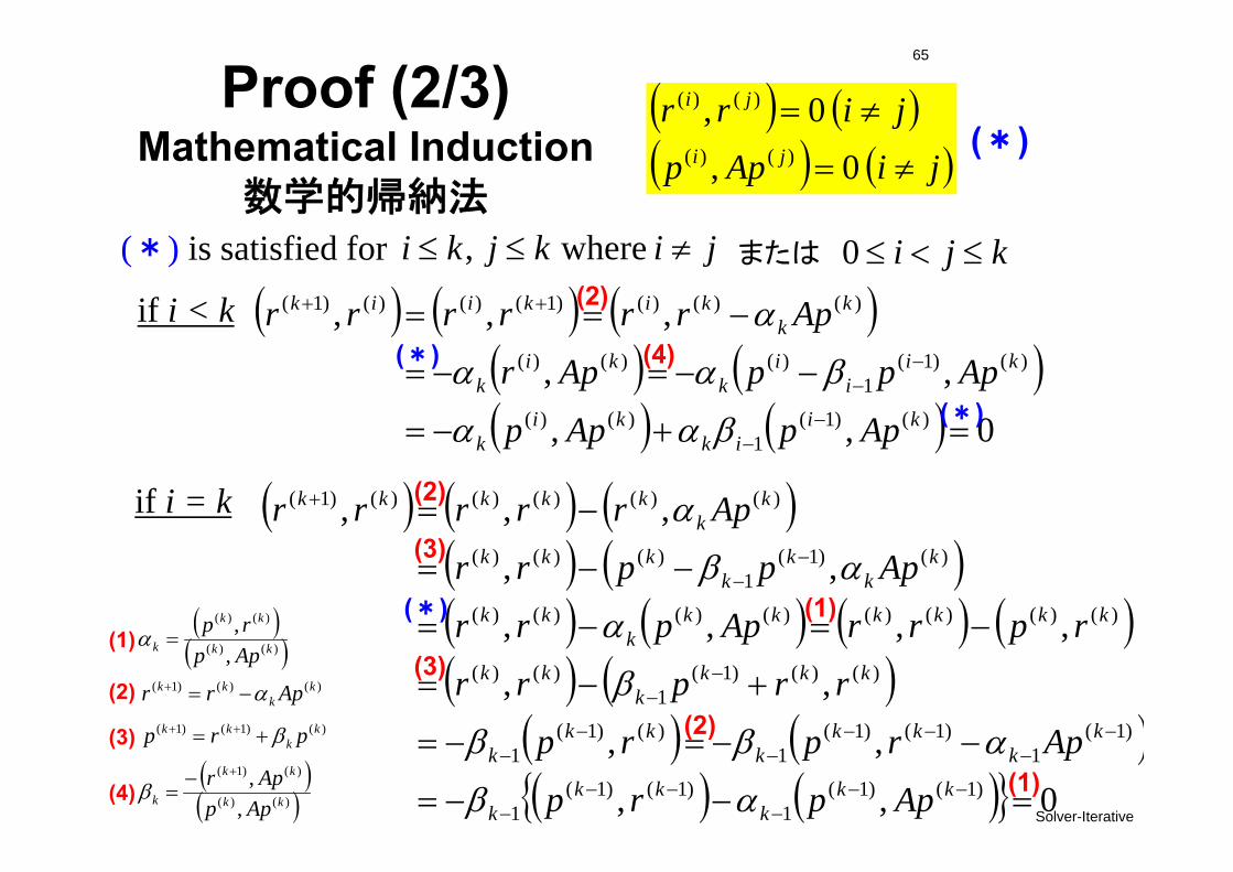
65
Proof (2/3)Mathematical Induction
数学的帰納法
Solver-Iterative
(*) is satisfied for jikjki where,
0,,
,,
,,,
)()1(1
)()(
)()1(1
)()()(
)()()()1()()()1(
kiik
kik
kii
ik
kik
kk
kikiik
AppApp
ApppApr
Aprrrrrr
jiApp
jirrji
ji
0,0,
)()(
)()(
if i < k
if i = k
0,,
,,
,,
,,,,
,,
,,,
)1()1(1
)1()1(1
)1(1
)1()1(1
)()1(1
)()()1(1
)()(
)()()()()()()()(
)()1(1
)()()(
)()()()()()1(
kkk
kkk
kk
kkk
kkk
kkkk
kk
kkkkkkk
kk
kk
kk
kkk
kk
kkkkk
Apprp
Aprprp
rrprr
rprrApprr
Appprr
Aprrrrr
(2)
(4)
(2)
(3)
(3)
(2)
(1)
(*)
(*)
(*)
(*) (1) )()(
)()(
,,
kk
kk
k Apprp
(1)
(2)
(3)
(4)
)()()1( kk
kk Aprr
)()1()1( kk
kk prp
)()(
)()1(
,,
kk
kk
k AppApr
kji 0または
66
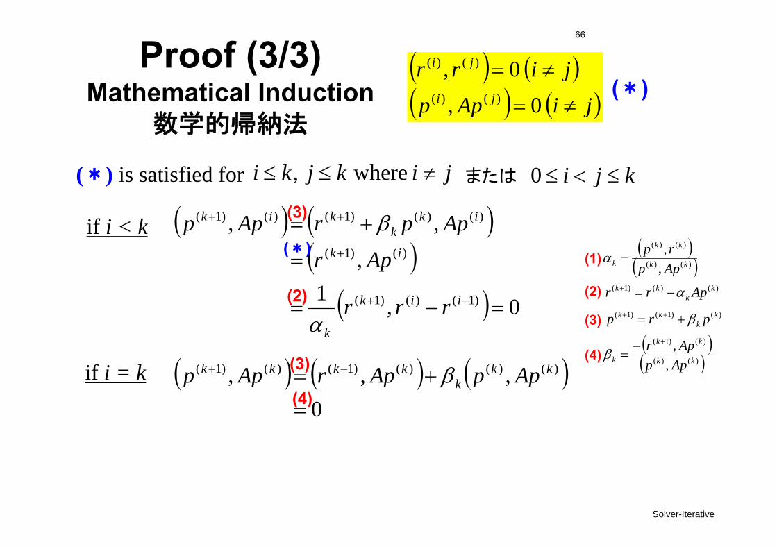
Proof (3/3)Mathematical Induction
数学的帰納法
Solver-Iterative
jiApp
jirrji
ji
0,0,
)()(
)()(
(*)
0
,,, )()()()1()()1(
kk
kkkkk AppAprApp
(*) is satisfied for
0,1,
,,
)1()()1(
)()1(
)()()1()()1(
iik
k
ik
ikk
kik
rrr
Apr
ApprApp
if i < k
if i = k
(3)
(2)
(3)
(4)
(*) )()(
)()(
,,
kk
kk
k Apprp
(1)
(2)
(3)
(4)
)()()1( kk
kk Aprr
)()1()1( kk
kk prp
)()(
)()1(
,,
kk
kk
k AppApr
jikjki where, kji 0または
67
Solver-Iterative
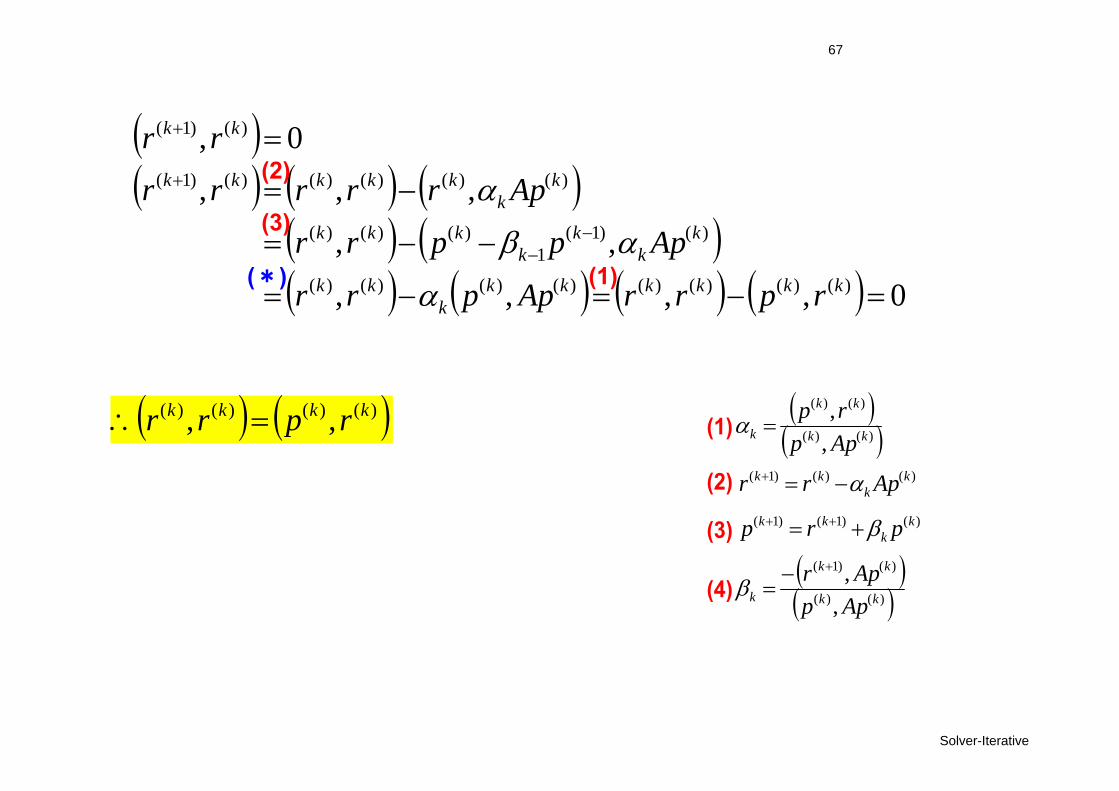
0,,,,
,,
,,,0,
)()()()()()()()(
)()1(1
)()()(
)()()()()()1(
)()1(
kkkkkkk
kk
kk
kk
kkk
kk
kkkkk
kk
rprrApprr
Appprr
Aprrrrrrr
(2)
(3)
(*) (1)
)()(
)()(
,,
kk
kk
k Apprp
(1)
(2)
(3)
(4)
)()()1( kk
kk Aprr
)()1()1( kk
kk prp
)()(
)()1(
,,
kk
kk
k AppApr
)()()()( ,, kkkk rprr
68
k,k
k
kk
k
kkkkk
kk
kk
kk
kk
k
rrrrrApr
rrrr
AppApr
)1()1()1()()1()()1(
)()(
)1()1(
)()(
)()1(
,,,
,,
,,
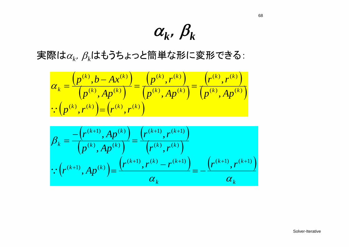
実際はk,kはもうちょっと簡単な形に変形できる:
)()()()(
)()(
)()(
)()(
)()(
)()(
)()(
,,,,
,,
,,
kkkk
kk
kk
kk
kk
kk
kk
k
rrrpApprr
Apprp
AppAxbp
Solver-Iterative
Solver-Iterative
69
共役勾配法(CG法)のアルゴリズム
Compute r(0)= b-[A]x(0)
for i= 1, 2, …i-1= r(i-1) r(i-1)if i=1p(1)= r(0)
elsei-1= i-1/i-2p(i)= r(i-1) + i-1 p(i-1)
endifq(i)= [A]p(i)
i = i-1/p(i)q(i)x(i)= x(i-1) + ip(i)r(i)= r(i-1) - iq(i)check convergence |r|
end
x(i) : Vectori : Scalar
)()(
)1()1(
,,
ii
ii
i Apprr
)2()2(
)1()1(
1 ,,
ii
ii
i rrrr
1 i 2 i
1 i
OMP-1 70
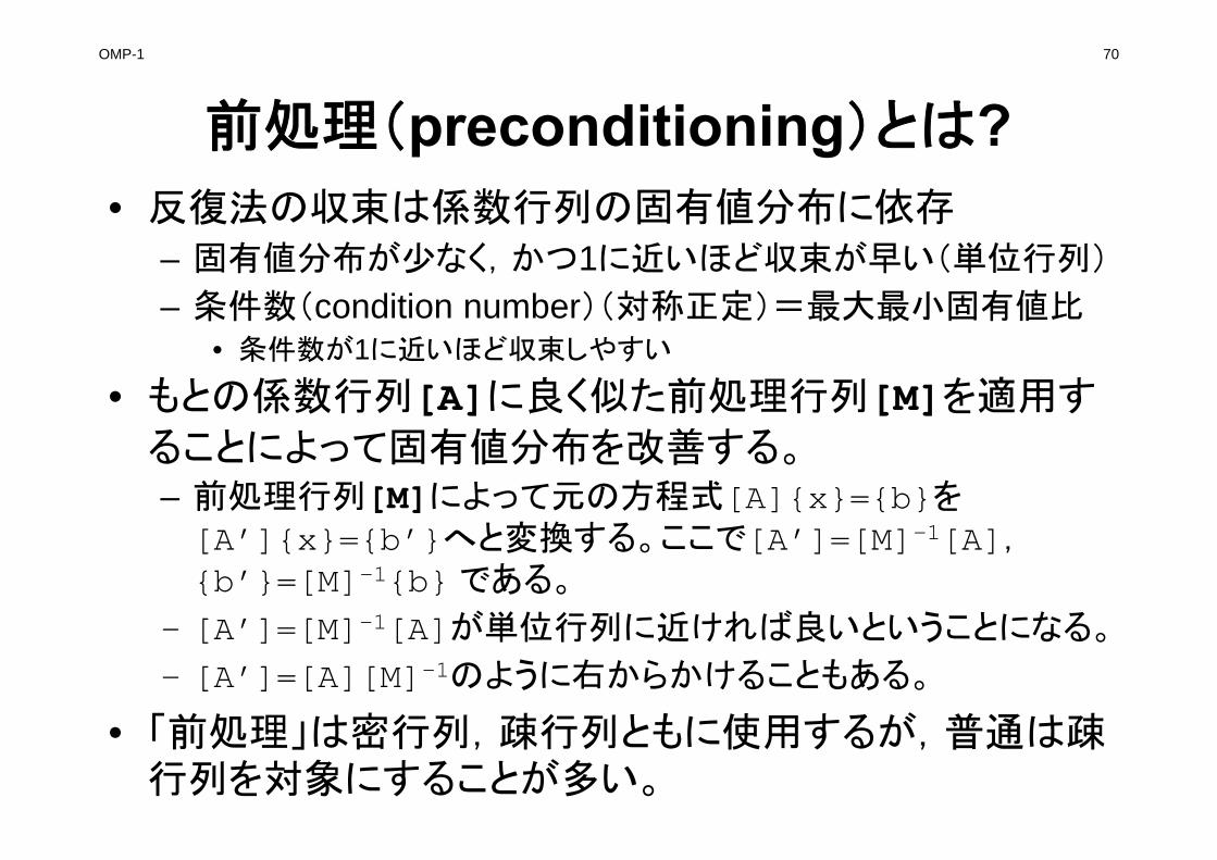
前処理(preconditioning)とは?• 反復法の収束は係数行列の固有値分布に依存
– 固有値分布が少なく,かつ1に近いほど収束が早い(単位行列)
– 条件数(condition number)(対称正定)= 大 小固有値比• 条件数が1に近いほど収束しやすい
• もとの係数行列[A]に良く似た前処理行列[M]を適用す
ることによって固有値分布を改善する。– 前処理行列[M]によって元の方程式[A]{x}={b}を[A’]{x}={b’}へと変換する。ここで[A’]=[M]-1[A],{b’}=[M]-1{b} である。
– [A’]=[M]-1[A]が単位行列に近ければ良いということになる。
– [A’]=[A][M]-1のように右からかけることもある。
• 「前処理」は密行列,疎行列ともに使用するが,普通は疎行列を対象にすることが多い。
OMP-1 71
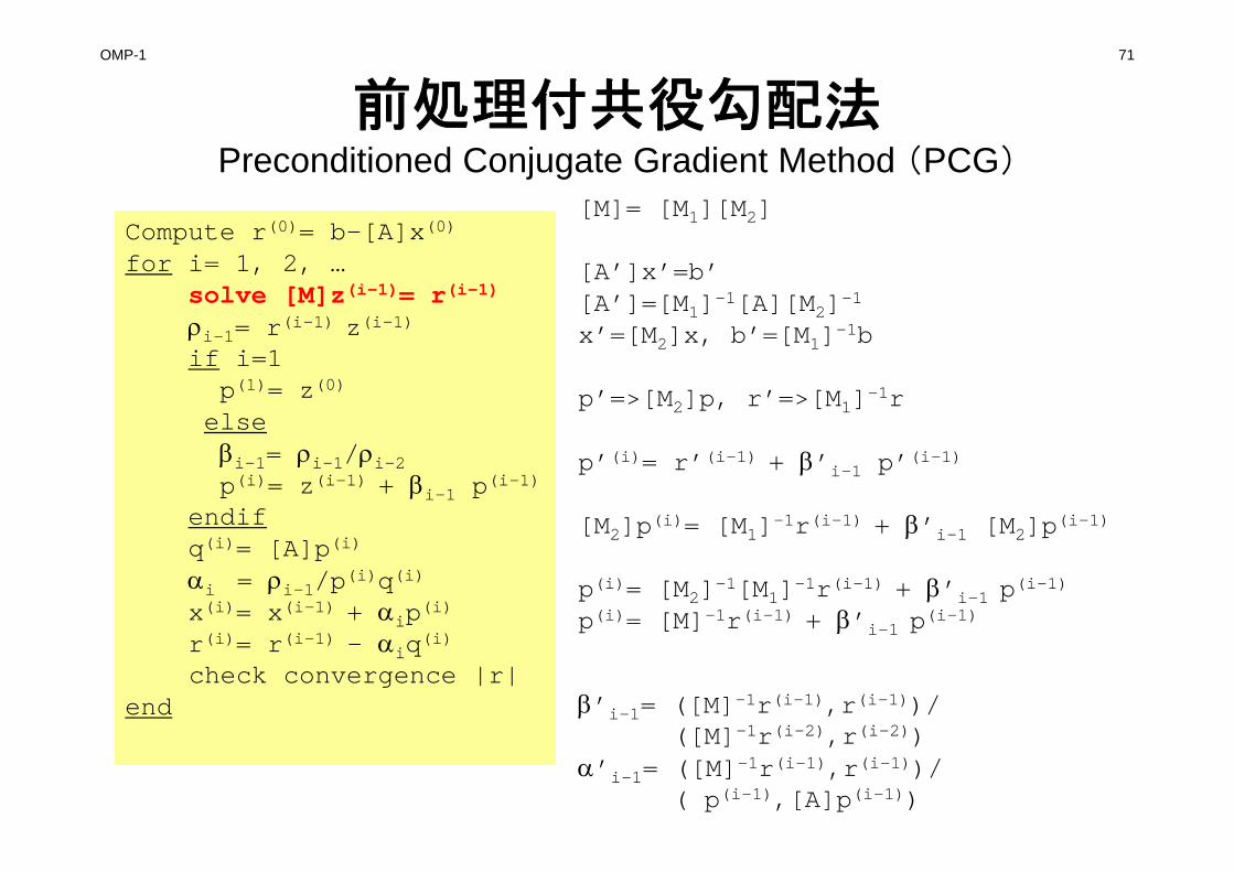
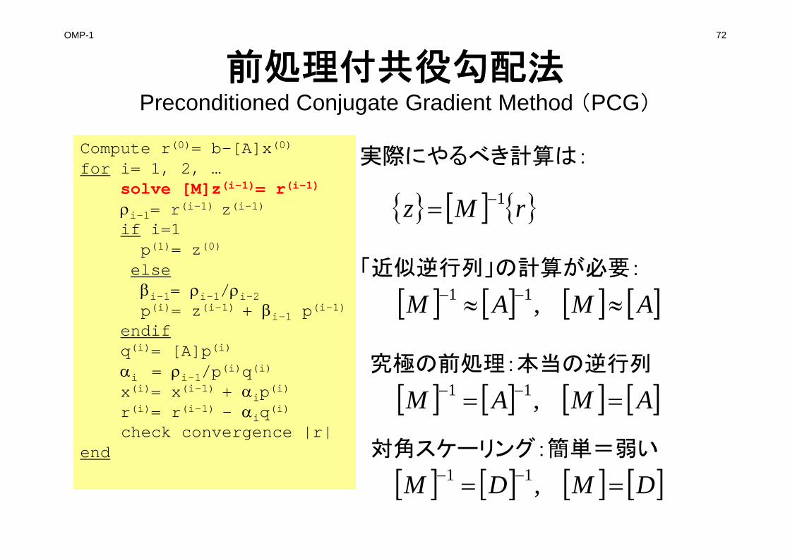
前処理付共役勾配法Preconditioned Conjugate Gradient Method (PCG)
Compute r(0)= b-[A]x(0)
for i= 1, 2, …solve [M]z(i-1)= r(i-1)
i-1= r(i-1) z(i-1)if i=1p(1)= z(0)
elsei-1= i-1/i-2p(i)= z(i-1) + i-1 p(i-1)
endifq(i)= [A]p(i)
i = i-1/p(i)q(i)x(i)= x(i-1) + ip(i)r(i)= r(i-1) - iq(i)check convergence |r|
end
[M]= [M1][M2]
[A’]x’=b’[A’]=[M1]-1[A][M2]-1
x’=[M2]x, b’=[M1]-1b
p’=>[M2]p, r’=>[M1]-1r
p’(i)= r’(i-1) + ’i-1 p’(i-1)
[M2]p(i)= [M1]-1r(i-1) + ’i-1 [M2]p(i-1)
p(i)= [M2]-1[M1]-1r(i-1) + ’i-1 p(i-1)p(i)= [M]-1r(i-1) + ’i-1 p(i-1)
’i-1= ([M]-1r(i-1),r(i-1))/([M]-1r(i-2),r(i-2))
’i-1= ([M]-1r(i-1),r(i-1))/( p(i-1),[A]p(i-1))
OMP-1 72
前処理付共役勾配法Preconditioned Conjugate Gradient Method (PCG)
Compute r(0)= b-[A]x(0)
for i= 1, 2, …solve [M]z(i-1)= r(i-1)
i-1= r(i-1) z(i-1)if i=1p(1)= z(0)
elsei-1= i-1/i-2p(i)= z(i-1) + i-1 p(i-1)
endifq(i)= [A]p(i)
i = i-1/p(i)q(i)x(i)= x(i-1) + ip(i)r(i)= r(i-1) - iq(i)check convergence |r|
end
実際にやるべき計算は:
rMz 1
AMAM ,11
対角スケーリング:簡単=弱い
DMDM ,11
究極の前処理:本当の逆行列
AMAM ,11
「近似逆行列」の計算が必要:
OMP-1 73
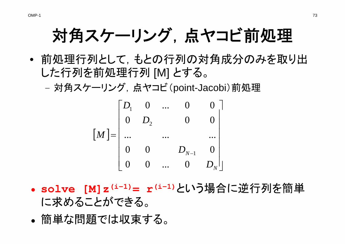
対角スケーリング,点ヤコビ前処理
• 前処理行列として,もとの行列の対角成分のみを取り出した行列を前処理行列 [M] とする。
– 対角スケーリング,点ヤコビ(point-Jacobi)前処理
N
N
DD
DD
M
0...00000.........00000...0
1
2
1
• solve [M]z(i-1)= r(i-1)という場合に逆行列を簡単に求めることができる。
• 簡単な問題では収束する。
OMP-1 74
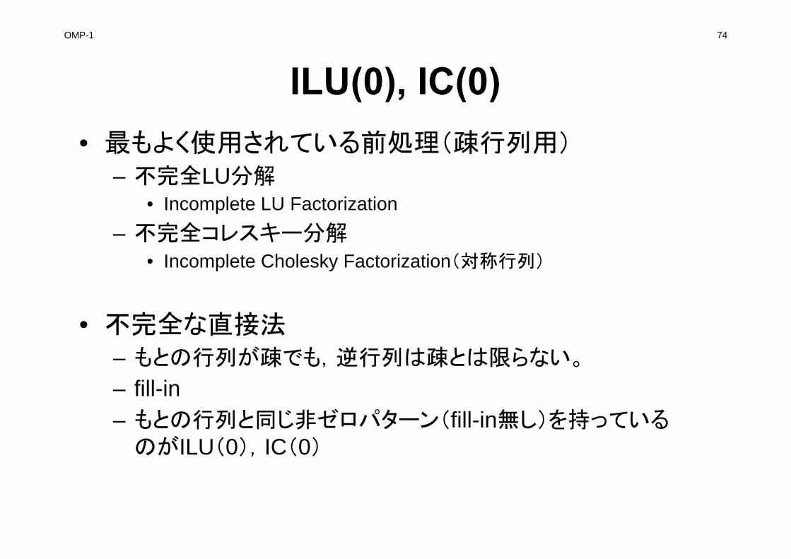
ILU(0), IC(0)• もよく使用されている前処理(疎行列用)
– 不完全LU分解• Incomplete LU Factorization
– 不完全コレスキー分解• Incomplete Cholesky Factorization(対称行列)
• 不完全な直接法– もとの行列が疎でも,逆行列は疎とは限らない。
– fill-in– もとの行列と同じ非ゼロパターン(fill-in無し)を持っている
のがILU(0),IC(0)
OMP-1 75
LU分解法:完全LU分解法
• 直接法の一種
– 逆行列を直接求める手法
– 「逆行列」に相当するものを保存しておけるので,右辺が変わったときに計算時間を節約できる
– 逆行列を求める際にFill-in(もとの行列では0であったところに値が入る)が生じる
• LU factorization
OMP-1 76
「不」完全LU分解法
• ILU factorization– Incomplete LU factorization
• Fill-inの発生を制限して,前処理に使う手法
– 不完全な逆行列,少し弱い直接法
– Fill-inを許さないとき:ILU(0)
OMP-1 77
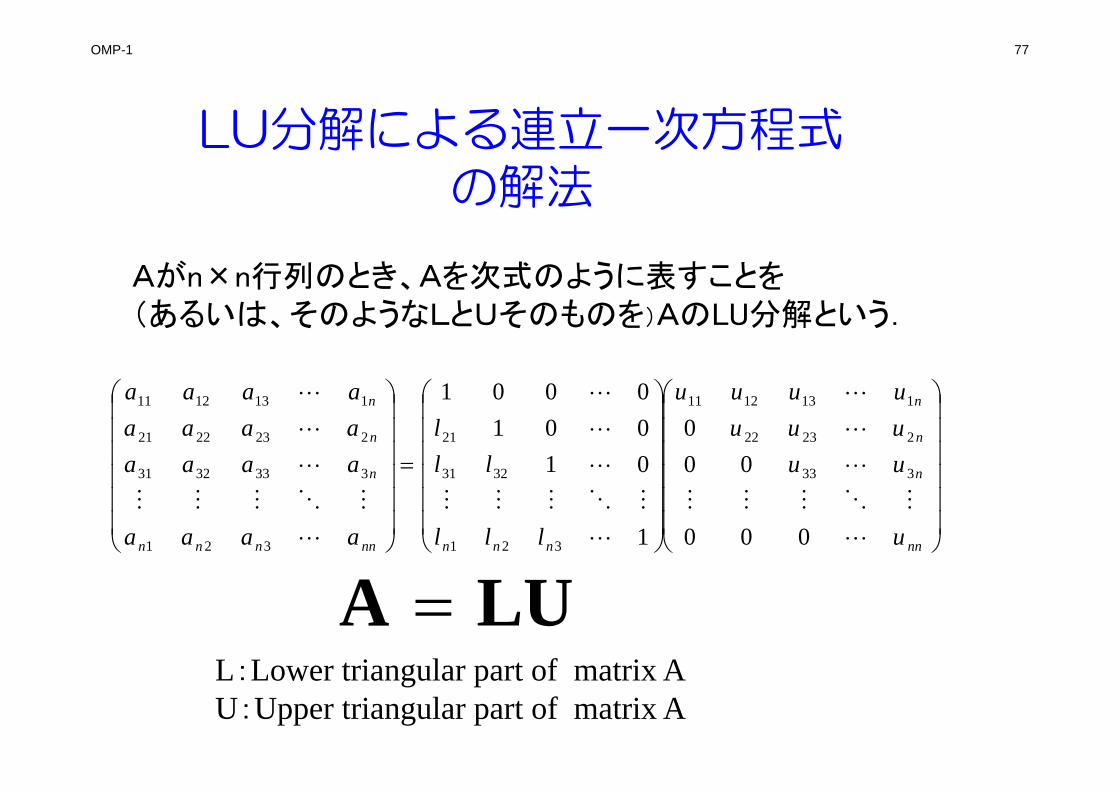
LU分解による連立一次方程式の解法
Aがn×n行列のとき、Aを次式のように表すことを(あるいは、そのようなLとUそのものを)AのLU分解という.
nn
n
n
n
nnnnnnnn
n
n
n
u
uuuuuuuuu
lll
lll
aaaa
aaaaaaaaaaaa
000
000
1
010010001
333
22322
1131211
321
3231
21
321
3333231
2232221
1131211
LUA L:Lower triangular part of matrix AU:Upper triangular part of matrix A
OMP-1 78
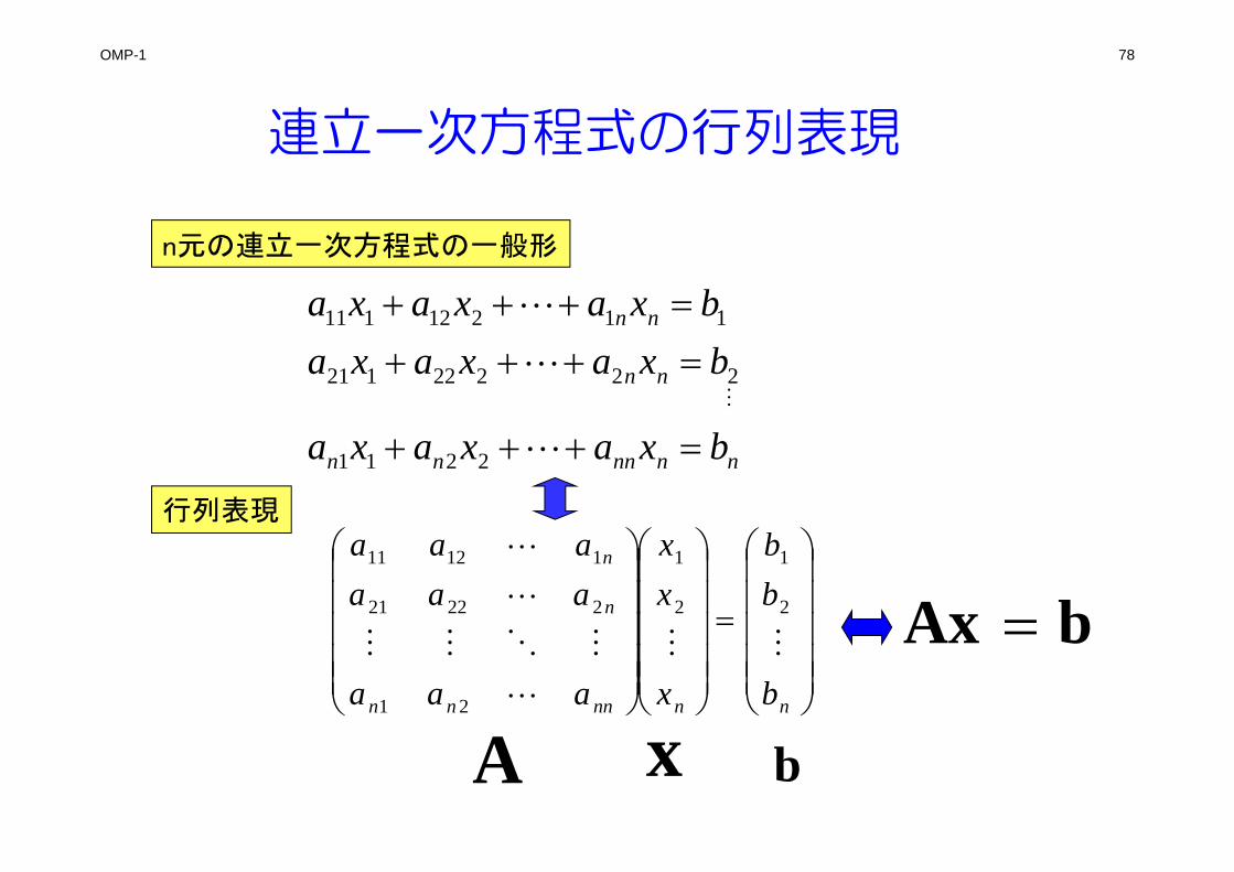
連立一次方程式の行列表現
n元の連立一次方程式の一般形
nnnnnn
nn
nn
bxaxaxa
bxaxaxabxaxaxa
2211
22222121
11212111
行列表現
nnnnnn
n
n
b
bb
x
xx
aaa
aaaaaa
2
1
2
1
21
22221
11211
A x b
bAx
OMP-1 79
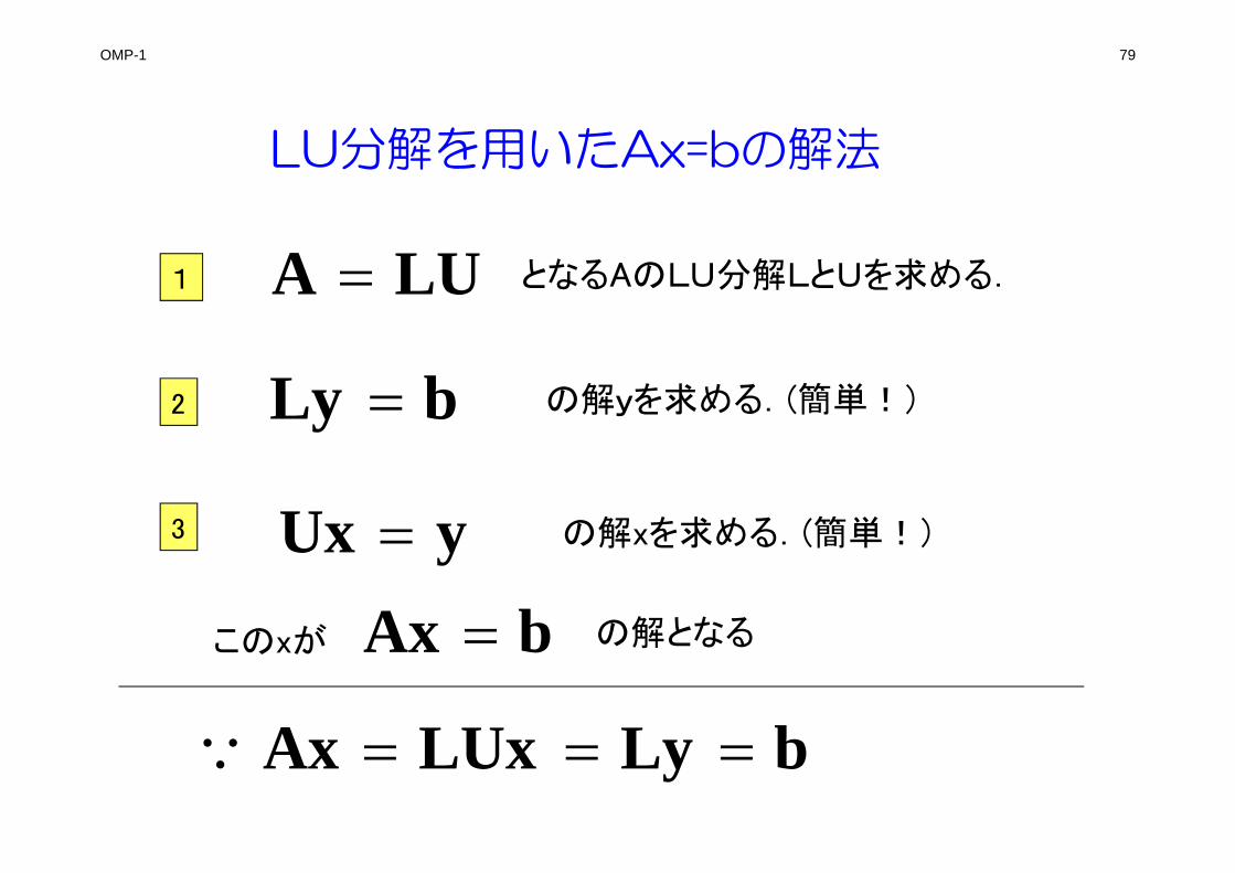
LU分解を用いたAx=bの解法
1
2
3
LUA となるAのLU分解LとUを求める.
bLy の解yを求める.(簡単!)
yUx の解xを求める.(簡単!)
このxが bAx の解となる
bLyLUxAx
OMP-1 80
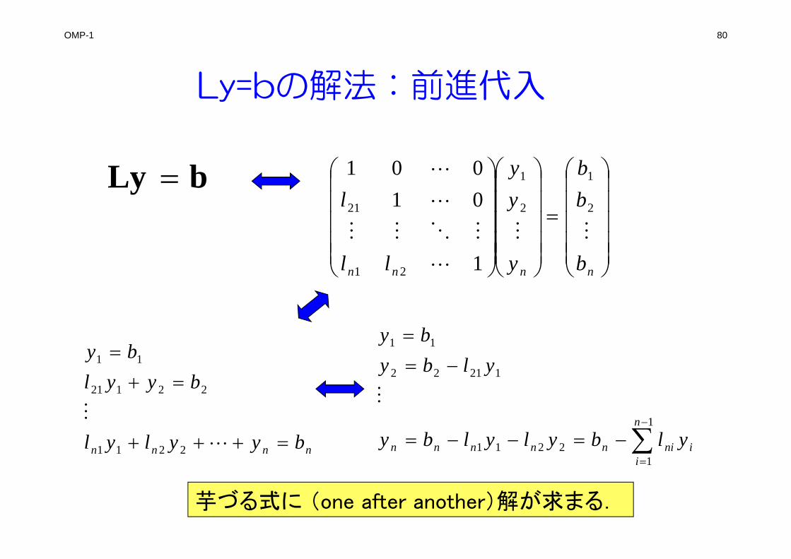
Ly=bの解法:前進代入
bLy
nnnn b
bb
y
yy
ll
l
2
1
2
1
21
21
1
01001
nnnn byylyl
byylby
2211
22121
11
i
n
ininnnnn ylbylylby
ylbyby
1
12211
12122
11
芋づる式に (one after another)解が求まる.
OMP-1 81
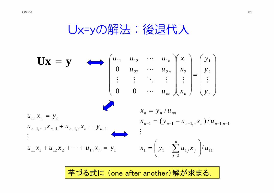
Ux=yの解法:後退代入
yUx
nnnn
n
n
y
yy
x
xx
u
uuuuu
2
1
2
1
222
11211
00
0
11212111
1,111,1
yxuxuxu
yxuxuyxu
nn
nnnnnnn
nnnn
112
111
1,1,111
/
/)(/
uxuyx
uxuyxuyx
j
n
ij
nnnnnnn
nnnn
芋づる式に (one after another)解が求まる.
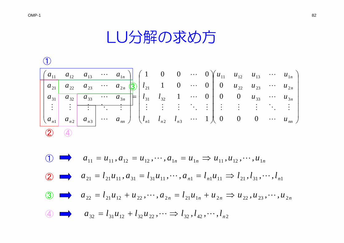
OMP-1 82
LU分解の求め方
nn
n
n
n
nnnnnnnn
n
n
n
u
uuuuuuuuu
lll
lll
aaaa
aaaaaaaaaaaa
000
000
1
010010001
333
22322
1131211
321
3231
21
321
3333231
2232221
1131211
①
②
③
④
①
②
③
④
nnn uuuuauaua 112111112121111 ,,,,,,
131211111113131112121 ,,,,,, nnn lllulaulaula
nnnn uuuuulauula 223222121222122122 ,,,,,
242322232123132 ,,,, nlllulula
OMP-1 83
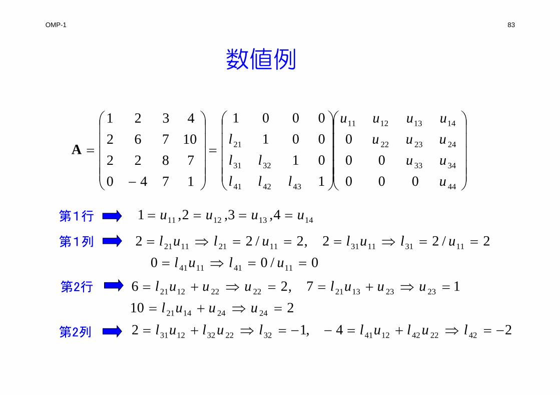
数値例
44
3433
242322
14131211
434241
3231
21
00000
0
1010010001
17407822
107624321
uuuuuuuuuu
lllll
lA
第1行 14131211 4,3,2,1 uuuu
第1列
0/002/22,2/22
11411141
1131113111211121
ulululululul
第2行
21017,26
24241421
2323132122221221
uuuluuuluuul
第2列 24,12 42224212413222321231 lulullulul
OMP-1 84
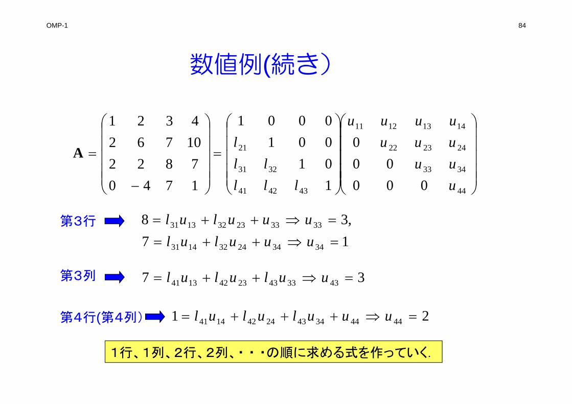
数値例(続き)
44
3433
242322
14131211
434241
3231
21
00000
0
1010010001
17407822
107624321
uuuuuuuuuu
lllll
lA
第3行
17,38
343424321431
333323321331
uuululuuulul
第3列 37 43334323421341 uululul
第4行(第4列) 21 4444344324421441 uuululul
1行、1列、2行、2列、・ ・ ・の順に求める式を作っていく.
OMP-1 85
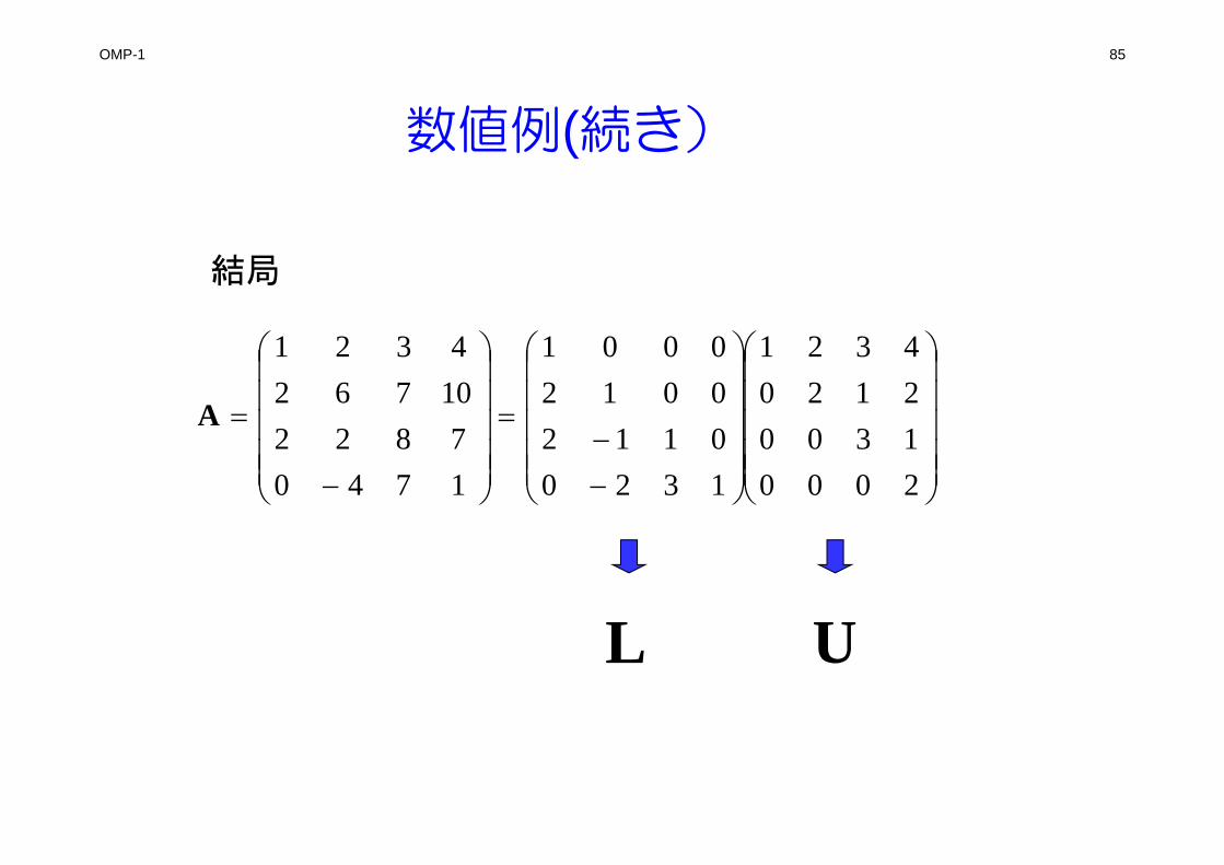
数値例(続き)
結局
2000130021204321
1320011200120001
17407822
107624321
A
L U
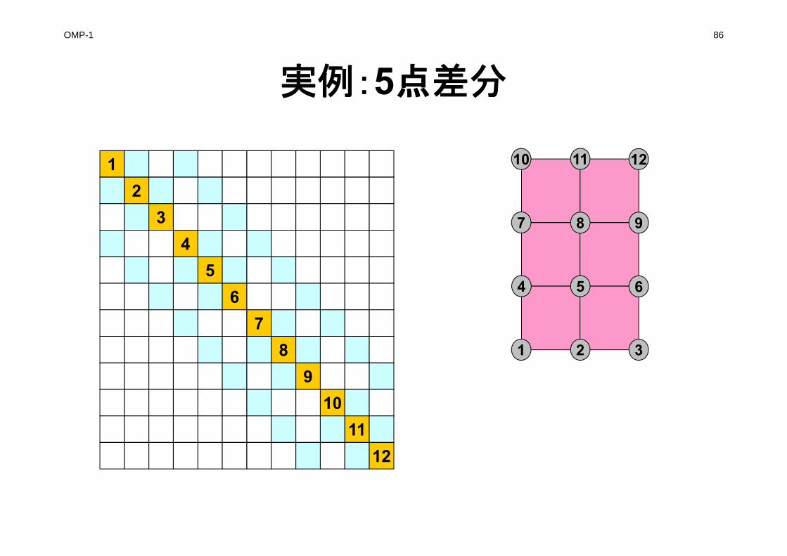
OMP-1 86
実例:5点差分
1
1 2 3
4 5 6
7 8 9
10 11 12
23
45
67
89
1011
12
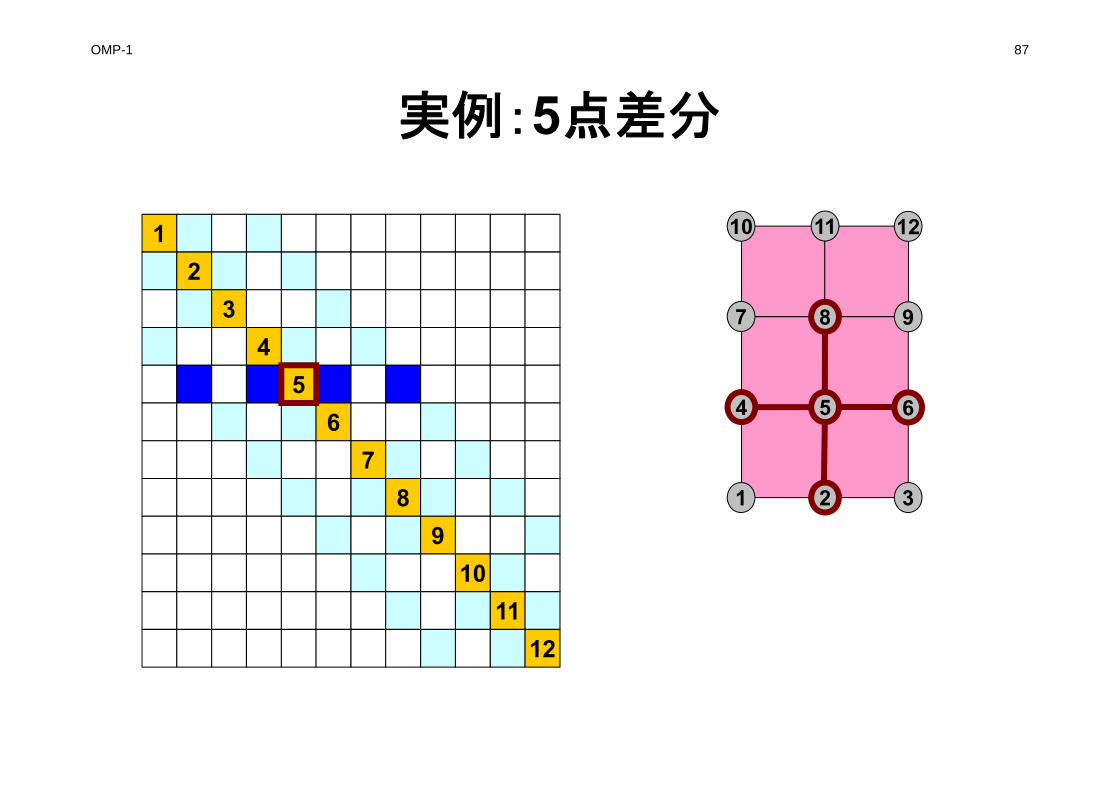
OMP-1 87
実例:5点差分
1
1 2 3
4 5 6
7 8 9
10 11 12
23
4
67
89
1011
12
5
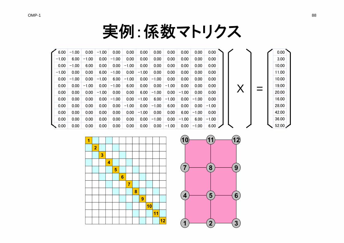
OMP-1 88
実例:係数マトリクス
1 2 3
4 5 6
7 8 9
10 11 1212
34
56
78
910
1112
=X
0.00
3.00
10.00
11.00
10.00
19.00
20.00
16.00
28.00
42.00
36.00
52.00
6.00 -1.00 0.00 -1.00 0.00 0.00 0.00 0.00 0.00 0.00 0.00 0.00
-1.00 6.00 -1.00 0.00 -1.00 0.00 0.00 0.00 0.00 0.00 0.00 0.00
0.00 -1.00 6.00 0.00 0.00 -1.00 0.00 0.00 0.00 0.00 0.00 0.00
-1.00 0.00 0.00 6.00 -1.00 0.00 -1.00 0.00 0.00 0.00 0.00 0.00
0.00 -1.00 0.00 -1.00 6.00 -1.00 0.00 -1.00 0.00 0.00 0.00 0.00
0.00 0.00 -1.00 0.00 -1.00 6.00 0.00 0.00 -1.00 0.00 0.00 0.00
0.00 0.00 0.00 -1.00 0.00 0.00 6.00 -1.00 0.00 -1.00 0.00 0.00
0.00 0.00 0.00 0.00 -1.00 0.00 -1.00 6.00 -1.00 0.00 -1.00 0.00
0.00 0.00 0.00 0.00 0.00 -1.00 0.00 -1.00 6.00 0.00 0.00 -1.00
0.00 0.00 0.00 0.00 0.00 0.00 -1.00 0.00 0.00 6.00 -1.00 0.00
0.00 0.00 0.00 0.00 0.00 0.00 0.00 -1.00 0.00 -1.00 6.00 -1.00
0.00 0.00 0.00 0.00 0.00 0.00 0.00 0.00 -1.00 0.00 -1.00 6.00
OMP-1 89
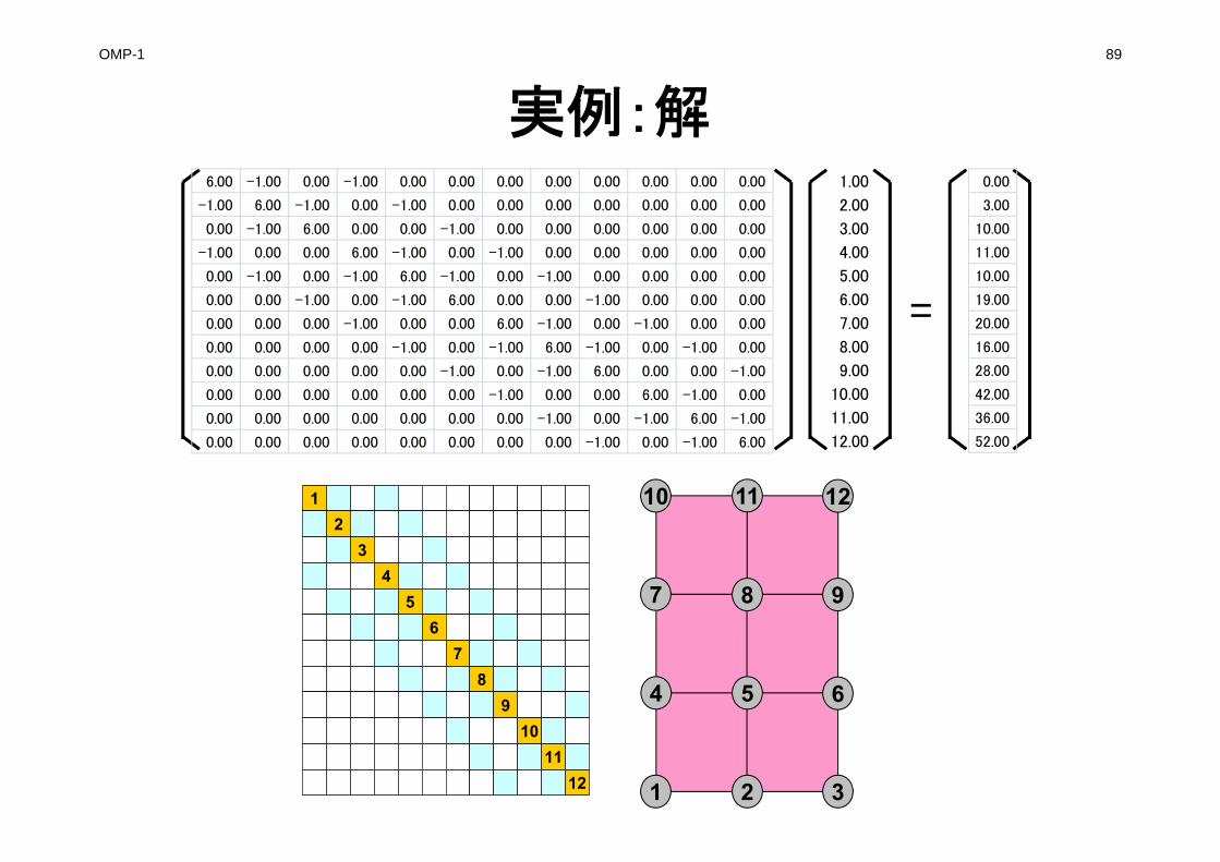
実例:解
1 2 3
4 5 6
7 8 9
10 11 1212
34
56
78
910
1112
=
6.00 -1.00 0.00 -1.00 0.00 0.00 0.00 0.00 0.00 0.00 0.00 0.00
-1.00 6.00 -1.00 0.00 -1.00 0.00 0.00 0.00 0.00 0.00 0.00 0.00
0.00 -1.00 6.00 0.00 0.00 -1.00 0.00 0.00 0.00 0.00 0.00 0.00
-1.00 0.00 0.00 6.00 -1.00 0.00 -1.00 0.00 0.00 0.00 0.00 0.00
0.00 -1.00 0.00 -1.00 6.00 -1.00 0.00 -1.00 0.00 0.00 0.00 0.00
0.00 0.00 -1.00 0.00 -1.00 6.00 0.00 0.00 -1.00 0.00 0.00 0.00
0.00 0.00 0.00 -1.00 0.00 0.00 6.00 -1.00 0.00 -1.00 0.00 0.00
0.00 0.00 0.00 0.00 -1.00 0.00 -1.00 6.00 -1.00 0.00 -1.00 0.00
0.00 0.00 0.00 0.00 0.00 -1.00 0.00 -1.00 6.00 0.00 0.00 -1.00
0.00 0.00 0.00 0.00 0.00 0.00 -1.00 0.00 0.00 6.00 -1.00 0.00
0.00 0.00 0.00 0.00 0.00 0.00 0.00 -1.00 0.00 -1.00 6.00 -1.00
0.00 0.00 0.00 0.00 0.00 0.00 0.00 0.00 -1.00 0.00 -1.00 6.00
1.00
2.00
3.00
4.00
5.00
6.00
7.00
8.00
9.00
10.00
11.00
12.00
0.00
3.00
10.00
11.00
10.00
19.00
20.00
16.00
28.00
42.00
36.00
52.00
OMP-1 90
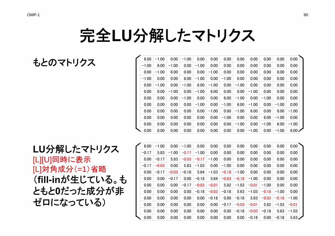
完全LU分解したマトリクス
もとのマトリクス
LU分解したマトリクス[L][U]同時に表示[L]対角成分(=1)省略
(fill-inが生じている。もともと0だった成分が非ゼロになっている)
6.00 -1.00 0.00 -1.00 0.00 0.00 0.00 0.00 0.00 0.00 0.00 0.00
-0.17 5.83 -1.00 -0.17 -1.00 0.00 0.00 0.00 0.00 0.00 0.00 0.00
0.00 -0.17 5.83 -0.03 -0.17 -1.00 0.00 0.00 0.00 0.00 0.00 0.00
-0.17 -0.03 0.00 5.83 -1.03 0.00 -1.00 0.00 0.00 0.00 0.00 0.00
0.00 -0.17 -0.03 -0.18 5.64 -1.03 -0.18 -1.00 0.00 0.00 0.00 0.00
0.00 0.00 -0.17 0.00 -0.18 5.64 -0.03 -0.18 -1.00 0.00 0.00 0.00
0.00 0.00 0.00 -0.17 -0.03 -0.01 5.82 -1.03 -0.01 -1.00 0.00 0.00
0.00 0.00 0.00 0.00 -0.18 -0.03 -0.18 5.63 -1.03 -0.18 -1.00 0.00
0.00 0.00 0.00 0.00 0.00 -0.18 0.00 -0.18 5.63 -0.03 -0.18 -1.00
0.00 0.00 0.00 0.00 0.00 0.00 -0.17 -0.03 -0.01 5.82 -1.03 -0.01
0.00 0.00 0.00 0.00 0.00 0.00 0.00 -0.18 -0.03 -0.18 5.63 -1.03
0.00 0.00 0.00 0.00 0.00 0.00 0.00 0.00 -0.18 0.00 -0.18 5.63
6.00 -1.00 0.00 -1.00 0.00 0.00 0.00 0.00 0.00 0.00 0.00 0.00
-1.00 6.00 -1.00 0.00 -1.00 0.00 0.00 0.00 0.00 0.00 0.00 0.00
0.00 -1.00 6.00 0.00 0.00 -1.00 0.00 0.00 0.00 0.00 0.00 0.00
-1.00 0.00 0.00 6.00 -1.00 0.00 -1.00 0.00 0.00 0.00 0.00 0.00
0.00 -1.00 0.00 -1.00 6.00 -1.00 0.00 -1.00 0.00 0.00 0.00 0.00
0.00 0.00 -1.00 0.00 -1.00 6.00 0.00 0.00 -1.00 0.00 0.00 0.00
0.00 0.00 0.00 -1.00 0.00 0.00 6.00 -1.00 0.00 -1.00 0.00 0.00
0.00 0.00 0.00 0.00 -1.00 0.00 -1.00 6.00 -1.00 0.00 -1.00 0.00
0.00 0.00 0.00 0.00 0.00 -1.00 0.00 -1.00 6.00 0.00 0.00 -1.00
0.00 0.00 0.00 0.00 0.00 0.00 -1.00 0.00 0.00 6.00 -1.00 0.00
0.00 0.00 0.00 0.00 0.00 0.00 0.00 -1.00 0.00 -1.00 6.00 -1.00
0.00 0.00 0.00 0.00 0.00 0.00 0.00 0.00 -1.00 0.00 -1.00 6.00
OMP-1 91
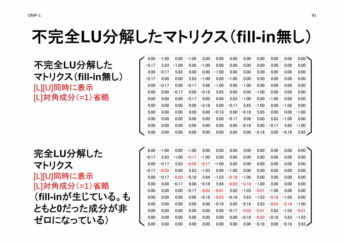
不完全LU分解したマトリクス(fill-in無し)
不完全LU分解したマトリクス(fill-in無し)[L][U]同時に表示[L]対角成分(=1)省略
完全LU分解したマトリクス[L][U]同時に表示[L]対角成分(=1)省略
(fill-inが生じている。もともと0だった成分が非ゼロになっている)
6.00 -1.00 0.00 -1.00 0.00 0.00 0.00 0.00 0.00 0.00 0.00 0.00
-0.17 5.83 -1.00 0.00 -1.00 0.00 0.00 0.00 0.00 0.00 0.00 0.00
0.00 -0.17 5.83 0.00 0.00 -1.00 0.00 0.00 0.00 0.00 0.00 0.00
-0.17 0.00 0.00 5.83 -1.00 0.00 -1.00 0.00 0.00 0.00 0.00 0.00
0.00 -0.17 0.00 -0.17 5.66 -1.00 0.00 -1.00 0.00 0.00 0.00 0.00
0.00 0.00 -0.17 0.00 -0.18 5.65 0.00 0.00 -1.00 0.00 0.00 0.00
0.00 0.00 0.00 -0.17 0.00 0.00 5.83 -1.00 0.00 -1.00 0.00 0.00
0.00 0.00 0.00 0.00 -0.18 0.00 -0.17 5.65 -1.00 0.00 -1.00 0.00
0.00 0.00 0.00 0.00 0.00 -0.18 0.00 -0.18 5.65 0.00 0.00 -1.00
0.00 0.00 0.00 0.00 0.00 0.00 -0.17 0.00 0.00 5.83 -1.00 0.00
0.00 0.00 0.00 0.00 0.00 0.00 0.00 -0.18 0.00 -0.17 5.65 -1.00
0.00 0.00 0.00 0.00 0.00 0.00 0.00 0.00 -0.18 0.00 -0.18 5.65
6.00 -1.00 0.00 -1.00 0.00 0.00 0.00 0.00 0.00 0.00 0.00 0.00
-0.17 5.83 -1.00 -0.17 -1.00 0.00 0.00 0.00 0.00 0.00 0.00 0.00
0.00 -0.17 5.83 -0.03 -0.17 -1.00 0.00 0.00 0.00 0.00 0.00 0.00
-0.17 -0.03 0.00 5.83 -1.03 0.00 -1.00 0.00 0.00 0.00 0.00 0.00
0.00 -0.17 -0.03 -0.18 5.64 -1.03 -0.18 -1.00 0.00 0.00 0.00 0.00
0.00 0.00 -0.17 0.00 -0.18 5.64 -0.03 -0.18 -1.00 0.00 0.00 0.00
0.00 0.00 0.00 -0.17 -0.03 -0.01 5.82 -1.03 -0.01 -1.00 0.00 0.00
0.00 0.00 0.00 0.00 -0.18 -0.03 -0.18 5.63 -1.03 -0.18 -1.00 0.00
0.00 0.00 0.00 0.00 0.00 -0.18 0.00 -0.18 5.63 -0.03 -0.18 -1.00
0.00 0.00 0.00 0.00 0.00 0.00 -0.17 -0.03 -0.01 5.82 -1.03 -0.01
0.00 0.00 0.00 0.00 0.00 0.00 0.00 -0.18 -0.03 -0.18 5.63 -1.03
0.00 0.00 0.00 0.00 0.00 0.00 0.00 0.00 -0.18 0.00 -0.18 5.63
OMP-1 92
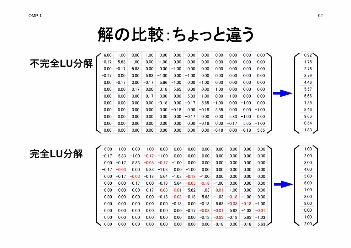
解の比較:ちょっと違う
不完全LU分解
完全LU分解
0.92
1.75
2.76
3.79
4.46
5.57
6.66
7.25
8.46
9.66
10.54
11.83
1.00
2.00
3.00
4.00
5.00
6.00
7.00
8.00
9.00
10.00
11.00
12.00
6.00 -1.00 0.00 -1.00 0.00 0.00 0.00 0.00 0.00 0.00 0.00 0.00
-0.17 5.83 -1.00 0.00 -1.00 0.00 0.00 0.00 0.00 0.00 0.00 0.00
0.00 -0.17 5.83 0.00 0.00 -1.00 0.00 0.00 0.00 0.00 0.00 0.00
-0.17 0.00 0.00 5.83 -1.00 0.00 -1.00 0.00 0.00 0.00 0.00 0.00
0.00 -0.17 0.00 -0.17 5.66 -1.00 0.00 -1.00 0.00 0.00 0.00 0.00
0.00 0.00 -0.17 0.00 -0.18 5.65 0.00 0.00 -1.00 0.00 0.00 0.00
0.00 0.00 0.00 -0.17 0.00 0.00 5.83 -1.00 0.00 -1.00 0.00 0.00
0.00 0.00 0.00 0.00 -0.18 0.00 -0.17 5.65 -1.00 0.00 -1.00 0.00
0.00 0.00 0.00 0.00 0.00 -0.18 0.00 -0.18 5.65 0.00 0.00 -1.00
0.00 0.00 0.00 0.00 0.00 0.00 -0.17 0.00 0.00 5.83 -1.00 0.00
0.00 0.00 0.00 0.00 0.00 0.00 0.00 -0.18 0.00 -0.17 5.65 -1.00
0.00 0.00 0.00 0.00 0.00 0.00 0.00 0.00 -0.18 0.00 -0.18 5.65
6.00 -1.00 0.00 -1.00 0.00 0.00 0.00 0.00 0.00 0.00 0.00 0.00
-0.17 5.83 -1.00 -0.17 -1.00 0.00 0.00 0.00 0.00 0.00 0.00 0.00
0.00 -0.17 5.83 -0.03 -0.17 -1.00 0.00 0.00 0.00 0.00 0.00 0.00
-0.17 -0.03 0.00 5.83 -1.03 0.00 -1.00 0.00 0.00 0.00 0.00 0.00
0.00 -0.17 -0.03 -0.18 5.64 -1.03 -0.18 -1.00 0.00 0.00 0.00 0.00
0.00 0.00 -0.17 0.00 -0.18 5.64 -0.03 -0.18 -1.00 0.00 0.00 0.00
0.00 0.00 0.00 -0.17 -0.03 -0.01 5.82 -1.03 -0.01 -1.00 0.00 0.00
0.00 0.00 0.00 0.00 -0.18 -0.03 -0.18 5.63 -1.03 -0.18 -1.00 0.00
0.00 0.00 0.00 0.00 0.00 -0.18 0.00 -0.18 5.63 -0.03 -0.18 -1.00
0.00 0.00 0.00 0.00 0.00 0.00 -0.17 -0.03 -0.01 5.82 -1.03 -0.01
0.00 0.00 0.00 0.00 0.00 0.00 0.00 -0.18 -0.03 -0.18 5.63 -1.03
0.00 0.00 0.00 0.00 0.00 0.00 0.00 0.00 -0.18 0.00 -0.18 5.63
OMP-1 93
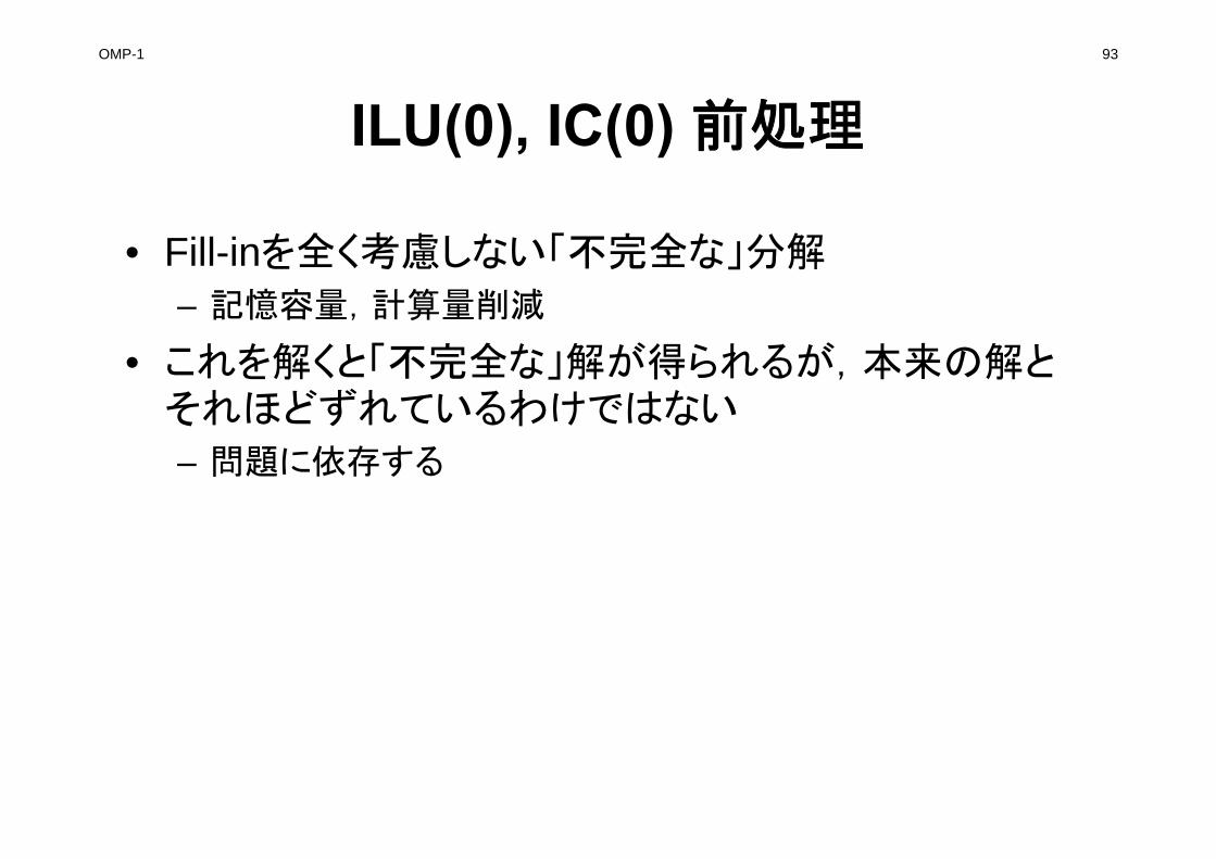
ILU(0), IC(0) 前処理
• Fill-inを全く考慮しない「不完全な」分解
– 記憶容量,計算量削減
• これを解くと「不完全な」解が得られるが,本来の解とそれほどずれているわけではない
– 問題に依存する
94
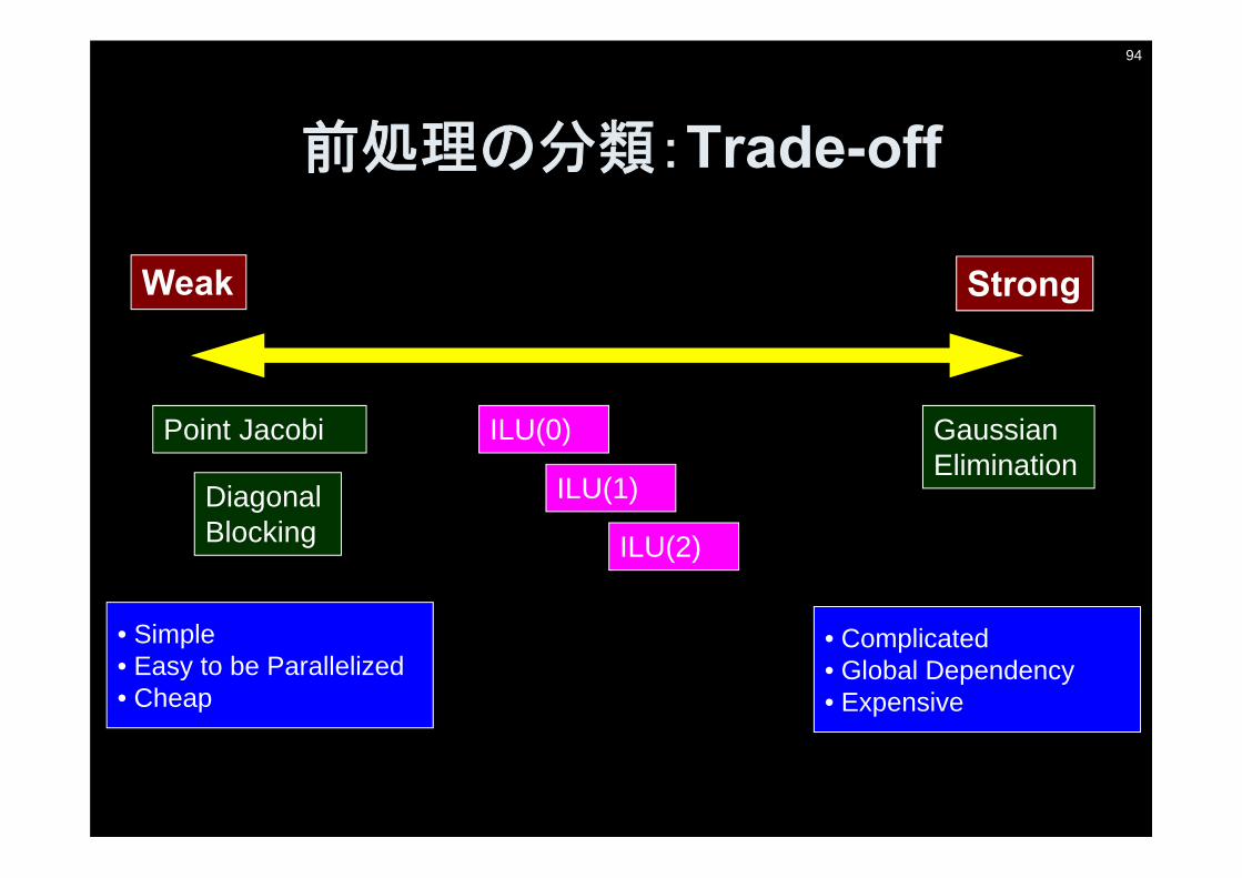
前処理の分類:Trade-off
Weak Strong
Gaussian Elimination
Point Jacobi
Diagonal Blocking
ILU(0)
ILU(1)
ILU(2)
• Simple • Easy to be Parallelized• Cheap
• Complicated• Global Dependency• Expensive
95
• 背景
– 有限体積法
– 前処理付反復法
• ICCG法によるポアソン方程式法ソルバーについて
– 実行方法• データ構造
– プログラムの説明• 初期化
• 係数マトリクス生成
• ICCG法
• OpenMP「超」入門
96
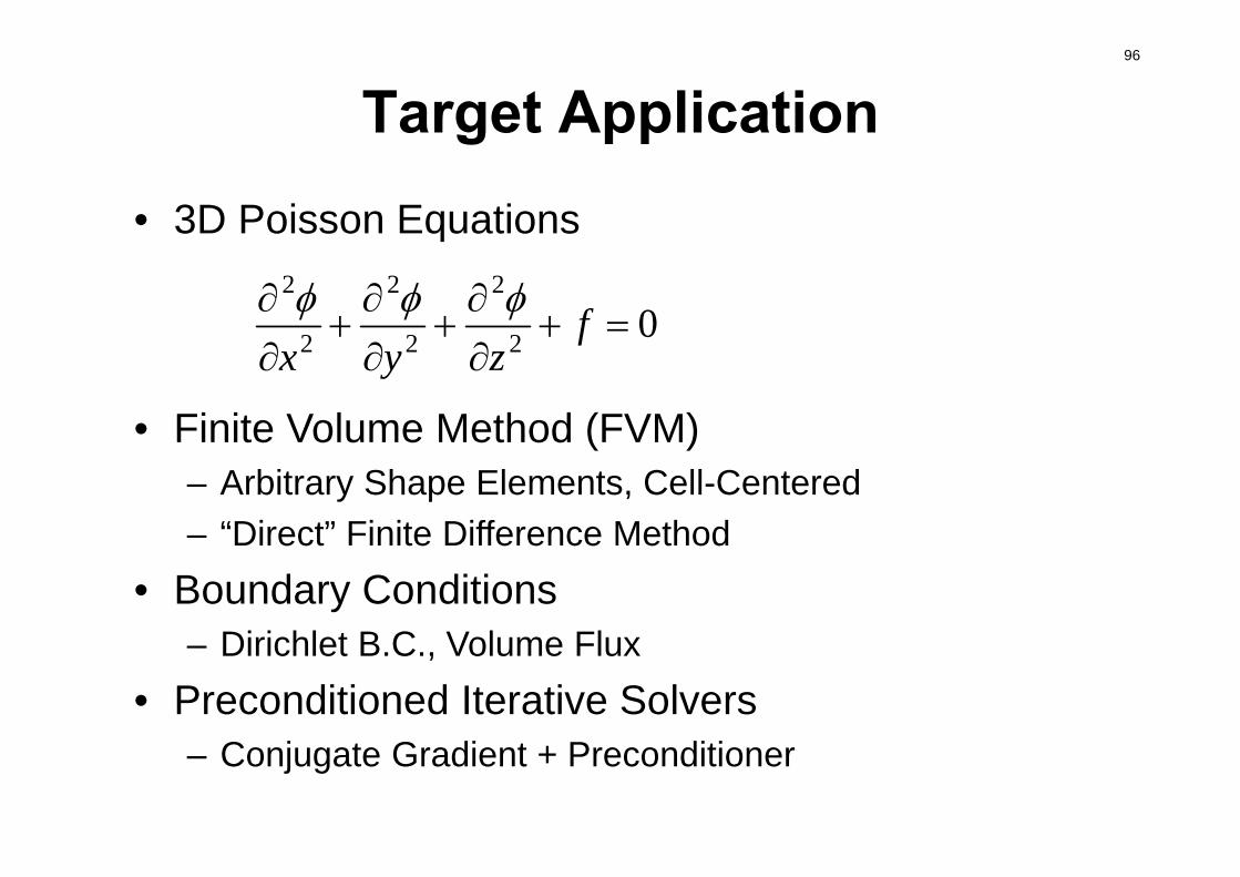
Target Application• 3D Poisson Equations
• Finite Volume Method (FVM)– Arbitrary Shape Elements, Cell-Centered– “Direct” Finite Difference Method
• Boundary Conditions– Dirichlet B.C., Volume Flux
• Preconditioned Iterative Solvers– Conjugate Gradient + Preconditioner
02
2
2
2
2
2
f
zyx
97
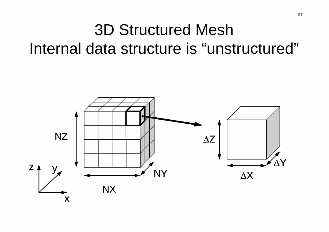
3D Structured MeshInternal data structure is “unstructured”
x
yz
NXNY
NZ Z
XY
x
yz
x
yz
NXNY
NZ Z
XY
Z
XY
XY
98
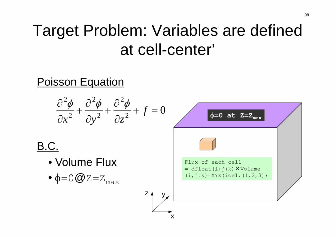
Target Problem: Variables are defined at cell-center’
x
yz
Poisson Equation
B.C.• Volume Flux• =0@Z=Zmax
Flux of each cell= dfloat(i+j+k)×Volume(i,j,k)=XYZ(icel,(1,2,3))
=0 at Z=Zmax02
2
2
2
2
2
f
zyx
99
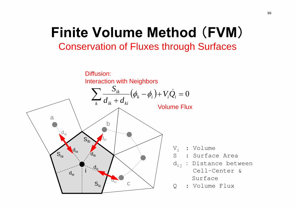
Finite Volume Method (FVM)Conservation of Fluxes through Surfaces
i
Sia
Sib
Sic
dia dib
dic
ab
c
dbi
dai
dci
0 ii
kik
kiik
ik QVdd
S
Vi : VolumeS : Surface Areadij : Distance between
Cell-Center & Surface
Q : Volume Flux
Diffusion:Interaction with Neighbors
Volume Flux
die
100
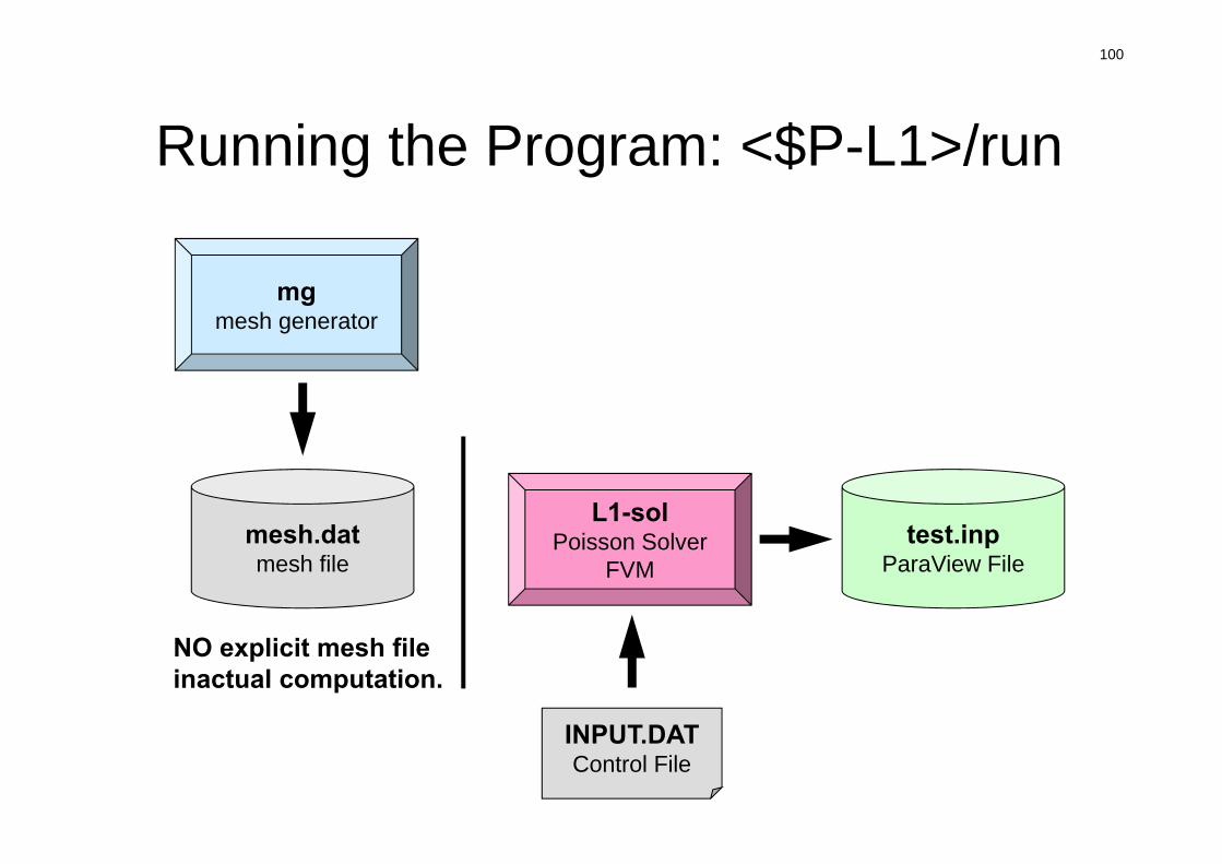
Running the Program: <$P-L1>/run
mgmesh generator
L1-solPoisson Solver
FVMmesh.datmesh file
INPUT.DATControl File
test.inpParaView File
NO explicit mesh fileinactual computation.
101
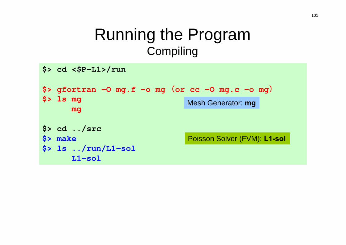
Running the ProgramCompiling
$> cd <$P-L1>/run
$> gfortran -O mg.f -o mg (or cc –O mg.c –o mg)$> ls mg
mg
$> cd ../src$> make$> ls ../run/L1-sol
L1-sol
Mesh Generator: mg
Poisson Solver (FVM): L1-sol
102
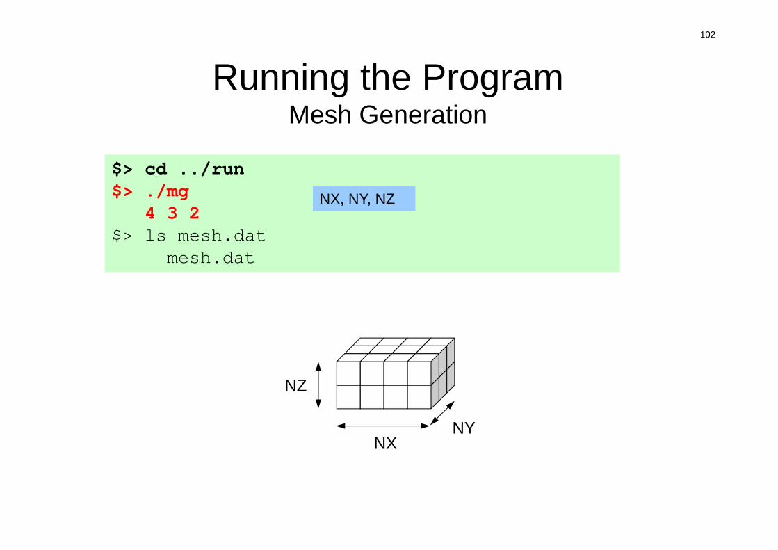
Running the ProgramMesh Generation
NXNY
NZ
$> cd ../run$> ./mg
4 3 2$> ls mesh.dat
mesh.dat
NX, NY, NZ
103
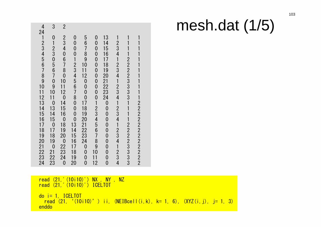
mesh.dat (1/5)4 3 2241 0 2 0 5 0 13 1 1 12 1 3 0 6 0 14 2 1 13 2 4 0 7 0 15 3 1 14 3 0 0 8 0 16 4 1 15 0 6 1 9 0 17 1 2 16 5 7 2 10 0 18 2 2 17 6 8 3 11 0 19 3 2 18 7 0 4 12 0 20 4 2 19 0 10 5 0 0 21 1 3 1
10 9 11 6 0 0 22 2 3 111 10 12 7 0 0 23 3 3 112 11 0 8 0 0 24 4 3 113 0 14 0 17 1 0 1 1 214 13 15 0 18 2 0 2 1 215 14 16 0 19 3 0 3 1 216 15 0 0 20 4 0 4 1 217 0 18 13 21 5 0 1 2 218 17 19 14 22 6 0 2 2 219 18 20 15 23 7 0 3 2 220 19 0 16 24 8 0 4 2 221 0 22 17 0 9 0 1 3 222 21 23 18 0 10 0 2 3 223 22 24 19 0 11 0 3 3 224 23 0 20 0 12 0 4 3 2
read (21,'(10i10)') NX , NY , NZread (21,'(10i10)') ICELTOT
do i= 1, ICELTOTread (21,‘(10i10)’) ii, (NEIBcell(i,k), k= 1, 6), (XYZ(i,j), j= 1, 3)
enddo
104
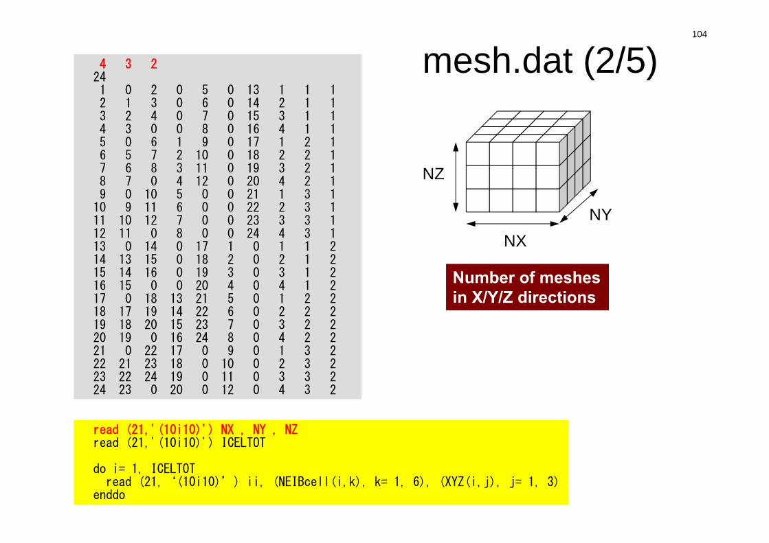
mesh.dat (2/5)4 3 2241 0 2 0 5 0 13 1 1 12 1 3 0 6 0 14 2 1 13 2 4 0 7 0 15 3 1 14 3 0 0 8 0 16 4 1 15 0 6 1 9 0 17 1 2 16 5 7 2 10 0 18 2 2 17 6 8 3 11 0 19 3 2 18 7 0 4 12 0 20 4 2 19 0 10 5 0 0 21 1 3 1
10 9 11 6 0 0 22 2 3 111 10 12 7 0 0 23 3 3 112 11 0 8 0 0 24 4 3 113 0 14 0 17 1 0 1 1 214 13 15 0 18 2 0 2 1 215 14 16 0 19 3 0 3 1 216 15 0 0 20 4 0 4 1 217 0 18 13 21 5 0 1 2 218 17 19 14 22 6 0 2 2 219 18 20 15 23 7 0 3 2 220 19 0 16 24 8 0 4 2 221 0 22 17 0 9 0 1 3 222 21 23 18 0 10 0 2 3 223 22 24 19 0 11 0 3 3 224 23 0 20 0 12 0 4 3 2
read (21,'(10i10)') NX , NY , NZread (21,'(10i10)') ICELTOT
do i= 1, ICELTOTread (21,‘(10i10)’) ii, (NEIBcell(i,k), k= 1, 6), (XYZ(i,j), j= 1, 3)
enddo
NXNY
NZ
Number of meshesin X/Y/Z directions
105
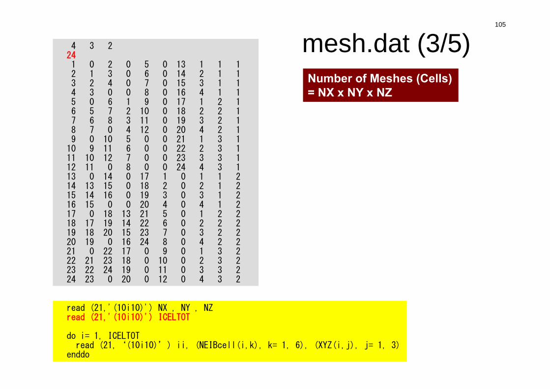
mesh.dat (3/5)4 3 2241 0 2 0 5 0 13 1 1 12 1 3 0 6 0 14 2 1 13 2 4 0 7 0 15 3 1 14 3 0 0 8 0 16 4 1 15 0 6 1 9 0 17 1 2 16 5 7 2 10 0 18 2 2 17 6 8 3 11 0 19 3 2 18 7 0 4 12 0 20 4 2 19 0 10 5 0 0 21 1 3 1
10 9 11 6 0 0 22 2 3 111 10 12 7 0 0 23 3 3 112 11 0 8 0 0 24 4 3 113 0 14 0 17 1 0 1 1 214 13 15 0 18 2 0 2 1 215 14 16 0 19 3 0 3 1 216 15 0 0 20 4 0 4 1 217 0 18 13 21 5 0 1 2 218 17 19 14 22 6 0 2 2 219 18 20 15 23 7 0 3 2 220 19 0 16 24 8 0 4 2 221 0 22 17 0 9 0 1 3 222 21 23 18 0 10 0 2 3 223 22 24 19 0 11 0 3 3 224 23 0 20 0 12 0 4 3 2
read (21,'(10i10)') NX , NY , NZread (21,'(10i10)') ICELTOT
do i= 1, ICELTOTread (21,‘(10i10)’) ii, (NEIBcell(i,k), k= 1, 6), (XYZ(i,j), j= 1, 3)
enddo
Number of Meshes (Cells)= NX x NY x NZ
106
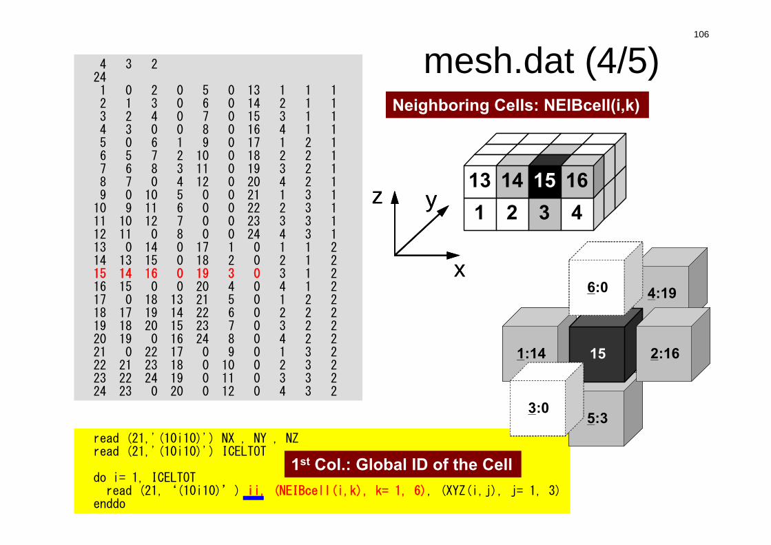
mesh.dat (4/5)4 3 2241 0 2 0 5 0 13 1 1 12 1 3 0 6 0 14 2 1 13 2 4 0 7 0 15 3 1 14 3 0 0 8 0 16 4 1 15 0 6 1 9 0 17 1 2 16 5 7 2 10 0 18 2 2 17 6 8 3 11 0 19 3 2 18 7 0 4 12 0 20 4 2 19 0 10 5 0 0 21 1 3 1
10 9 11 6 0 0 22 2 3 111 10 12 7 0 0 23 3 3 112 11 0 8 0 0 24 4 3 113 0 14 0 17 1 0 1 1 214 13 15 0 18 2 0 2 1 215 14 16 0 19 3 0 3 1 216 15 0 0 20 4 0 4 1 217 0 18 13 21 5 0 1 2 218 17 19 14 22 6 0 2 2 219 18 20 15 23 7 0 3 2 220 19 0 16 24 8 0 4 2 221 0 22 17 0 9 0 1 3 222 21 23 18 0 10 0 2 3 223 22 24 19 0 11 0 3 3 224 23 0 20 0 12 0 4 3 2
read (21,'(10i10)') NX , NY , NZread (21,'(10i10)') ICELTOT
do i= 1, ICELTOTread (21,‘(10i10)’) ii, (NEIBcell(i,k), k= 1, 6), (XYZ(i,j), j= 1, 3)
enddo
Neighboring Cells: NEIBcell(i,k)
x
yz
x
yz1 2 3 4 13 14 15 16
4:19
1:14
5:3
15
6:0
2:16
3:0
4:19
1:14
5:3
15
6:0
2:16
3:0
1st Col.: Global ID of the Cell

107
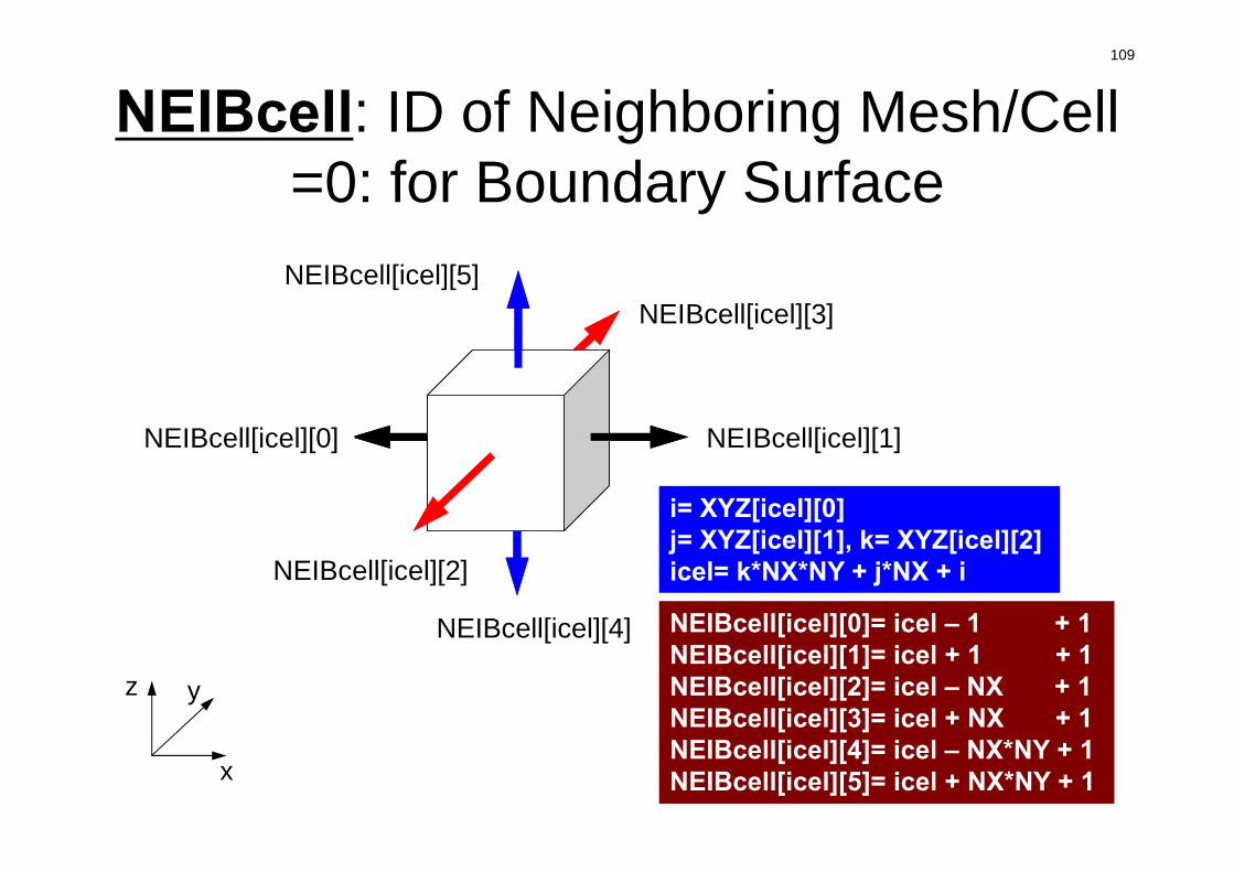
NEIBcell: ID of Neighboring Mesh/Cell=0: for Boundary Surface
NEIBcell(icel,2)NEIBcell(icel,1)
NEIBcell(icel,3)
NEIBcell(icel,5)
NEIBcell(icel,4)NEIBcell(icel,6)
NEIBcell(icel,2)NEIBcell(icel,1)
NEIBcell(icel,3)
NEIBcell(icel,5)
NEIBcell(icel,4)NEIBcell(icel,6)
NEIBcell[icel][3]
NEIBcell[icel][1]NEIBcell[icel][0]
NEIBcell[icel][2]
NEIBcell[icel][4]
NEIBcell[icel][5]
i= XYZ[icel][0]j= XYZ[icel][1], k= XYZ[icel][2]icel= k*NX*NY + j*NX + i
NEIBcell[icel][0]= icel – 1 + 1 NEIBcell[icel][1]= icel + 1 + 1NEIBcell[icel][2]= icel – NX + 1NEIBcell[icel][3]= icel + NX + 1NEIBcell[icel][4]= icel – NX*NY + 1NEIBcell[icel][5]= icel + NX*NY + 1
108
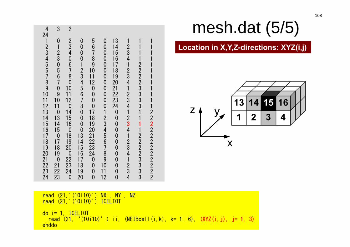
mesh.dat (5/5)4 3 2241 0 2 0 5 0 13 1 1 12 1 3 0 6 0 14 2 1 13 2 4 0 7 0 15 3 1 14 3 0 0 8 0 16 4 1 15 0 6 1 9 0 17 1 2 16 5 7 2 10 0 18 2 2 17 6 8 3 11 0 19 3 2 18 7 0 4 12 0 20 4 2 19 0 10 5 0 0 21 1 3 1
10 9 11 6 0 0 22 2 3 111 10 12 7 0 0 23 3 3 112 11 0 8 0 0 24 4 3 113 0 14 0 17 1 0 1 1 214 13 15 0 18 2 0 2 1 215 14 16 0 19 3 0 3 1 216 15 0 0 20 4 0 4 1 217 0 18 13 21 5 0 1 2 218 17 19 14 22 6 0 2 2 219 18 20 15 23 7 0 3 2 220 19 0 16 24 8 0 4 2 221 0 22 17 0 9 0 1 3 222 21 23 18 0 10 0 2 3 223 22 24 19 0 11 0 3 3 224 23 0 20 0 12 0 4 3 2
read (21,'(10i10)') NX , NY , NZread (21,'(10i10)') ICELTOT
do i= 1, ICELTOTread (21,‘(10i10)’) ii, (NEIBcell(i,k), k= 1, 6), (XYZ(i,j), j= 1, 3)
enddo
Location in X,Y,Z-directions: XYZ(i,j)
x
yz
x
yz1 2 3 4 13 14 15 16
109
NEIBcell: ID of Neighboring Mesh/Cell=0: for Boundary Surface
x
yz
NEIBcell(icel,2)NEIBcell(icel,1)
NEIBcell(icel,3)
NEIBcell(icel,5)
NEIBcell(icel,4)NEIBcell(icel,6)
NEIBcell(icel,2)NEIBcell(icel,1)
NEIBcell(icel,3)
NEIBcell(icel,5)
NEIBcell(icel,4)NEIBcell(icel,6)
NEIBcell[icel][3]
NEIBcell[icel][1]NEIBcell[icel][0]
NEIBcell[icel][2]
NEIBcell[icel][4]
NEIBcell[icel][5]
i= XYZ[icel][0]j= XYZ[icel][1], k= XYZ[icel][2]icel= k*NX*NY + j*NX + i
NEIBcell[icel][0]= icel – 1 + 1 NEIBcell[icel][1]= icel + 1 + 1NEIBcell[icel][2]= icel – NX + 1NEIBcell[icel][3]= icel + NX + 1NEIBcell[icel][4]= icel – NX*NY + 1NEIBcell[icel][5]= icel + NX*NY + 1
110
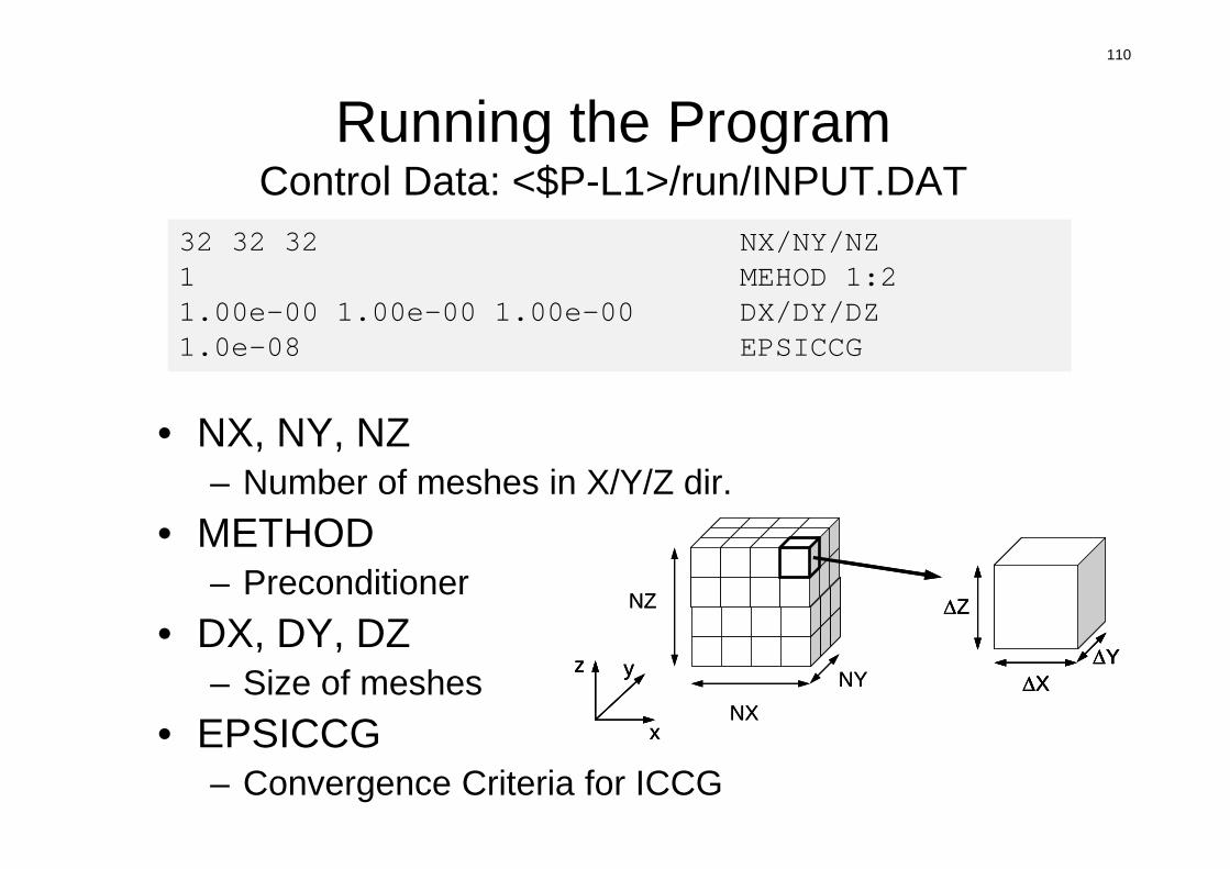
Running the ProgramControl Data: <$P-L1>/run/INPUT.DAT
• NX, NY, NZ– Number of meshes in X/Y/Z dir.
• METHOD– Preconditioner
• DX, DY, DZ– Size of meshes
• EPSICCG– Convergence Criteria for ICCG
32 32 32 NX/NY/NZ1 MEHOD 1:21.00e-00 1.00e-00 1.00e-00 DX/DY/DZ1.0e-08 EPSICCG
x
yz
NXNY
NZ Z
XY
x
yz
x
yz
NXNY
NZ Z
XY
Z
XY
XY
111
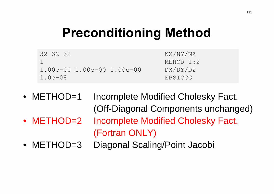
Preconditioning Method
• METHOD=1 Incomplete Modified Cholesky Fact.(Off-Diagonal Components unchanged)
• METHOD=2 Incomplete Modified Cholesky Fact.(Fortran ONLY)
• METHOD=3 Diagonal Scaling/Point Jacobi
32 32 32 NX/NY/NZ1 MEHOD 1:21.00e-00 1.00e-00 1.00e-00 DX/DY/DZ1.0e-08 EPSICCG
OMP-1 112
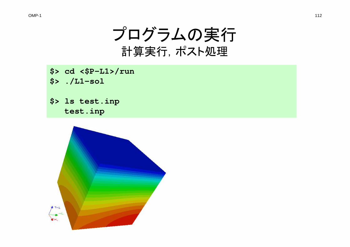
プログラムの実行計算実行,ポスト処理
$> cd <$P-L1>/run$> ./L1-sol
$> ls test.inptest.inp
ParaView• ファイルを開く
• 図の表示
• イメージファイルの保存
FEM3D-Part1 113
114
114
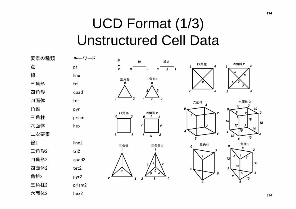
UCD Format (1/3)Unstructured Cell Data
要素の種類 キーワード
点 pt
線 line
三角形 tri
四角形 quad
四面体 tet
角錐 pyr
三角柱 prism
六面体 hex
二次要素
線2 line2
三角形2 tri2
四角形2 quad2
四面体2 tet2
角錐2 pyr2
三角柱2 prism2
六面体2 hex2
115
115
UCD Format (2/3)
• Originally for AVS, microAVS• Extension of the UCD file is “inp”• There are two types of formats. Only old type can
be read by ParaView.
116
116
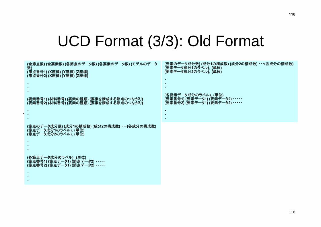
UCD Format (3/3): Old Format(全節点数) (全要素数) (各節点のデータ数) (各要素のデータ数) (モデルのデータ数)(節点番号1) (X座標) (Y座標) (Z座標) (節点番号2) (X座標) (Y座標) (Z座標)
・・・
(要素番号1) (材料番号) (要素の種類) (要素を構成する節点のつながり) (要素番号2) (材料番号) (要素の種類) (要素を構成する節点のつながり)
・・・
(節点のデータ成分数) (成分1の構成数) (成分2の構成数) ・・・(各成分の構成数)(節点データ成分1のラベル),(単位)(節点データ成分2のラベル),(単位)
・・・
(各節点データ成分のラベル),(単位)(節点番号1) (節点データ1) (節点データ2) ・・・・・(節点番号2) (節点データ1) (節点データ2) ・・・・・
・・・
(要素のデータ成分数) (成分1の構成数) (成分2の構成数) ・・・(各成分の構成数)(要素データ成分1のラベル),(単位)(要素データ成分2のラベル),(単位)
・・・
(各要素データ成分のラベル),(単位)(要素番号1) (要素データ1) (要素データ2) ・・・・・(要素番号2) (要素データ1) (要素データ2) ・・・・・
・・・
117
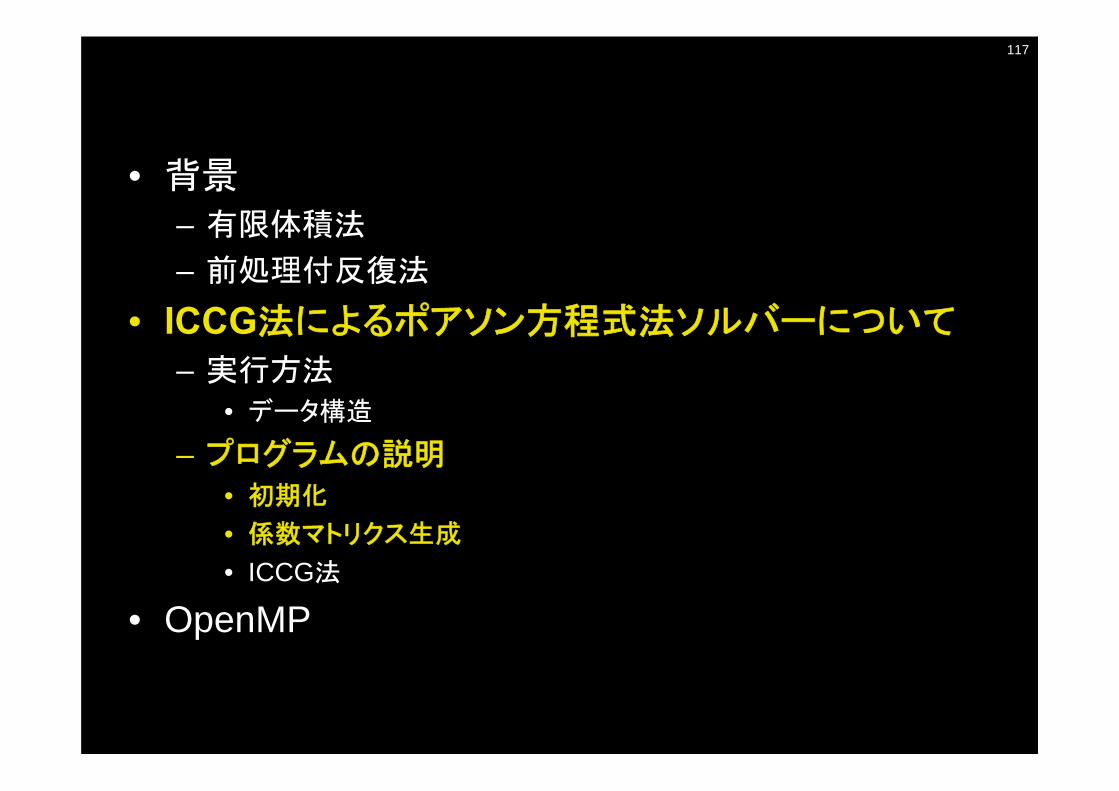
• 背景
– 有限体積法
– 前処理付反復法
• ICCG法によるポアソン方程式法ソルバーについて
– 実行方法• データ構造
– プログラムの説明• 初期化
• 係数マトリクス生成
• ICCG法
• OpenMP
118
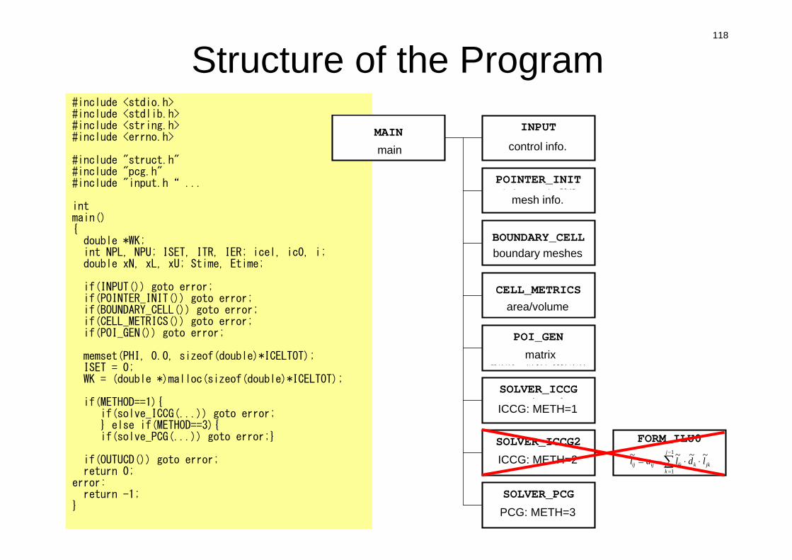
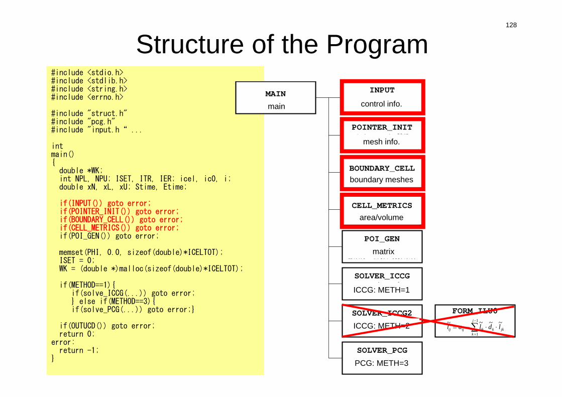
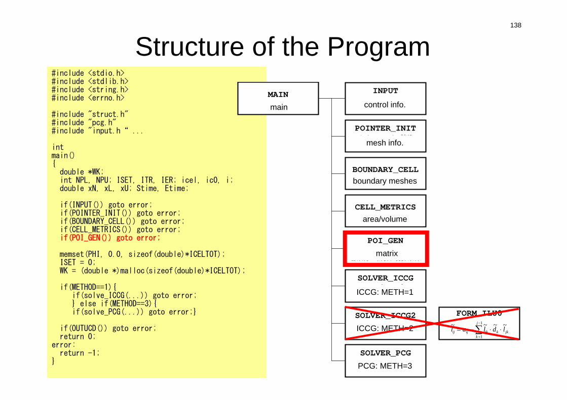
Structure of the Program#include <stdio.h>#include <stdlib.h>#include <string.h>#include <errno.h>
#include "struct.h"#include "pcg.h"#include "input.h“ ...
intmain(){double *WK;int NPL, NPU; ISET, ITR, IER; icel, ic0, i;double xN, xL, xU; Stime, Etime;
if(INPUT()) goto error;if(POINTER_INIT()) goto error;if(BOUNDARY_CELL()) goto error;if(CELL_METRICS()) goto error;if(POI_GEN()) goto error;
memset(PHI, 0.0, sizeof(double)*ICELTOT);ISET = 0;WK = (double *)malloc(sizeof(double)*ICELTOT);
if(METHOD==1){if(solve_ICCG(...)) goto error;} else if(METHOD==3){if(solve_PCG(...)) goto error;}
if(OUTUCD()) goto error;return 0;
error:return -1;
}
MAINメインルーチン
INPUT制御ファイル読込INPUT.DAT
POINTER_INITメッシュファイル読込
mesh.dat
BOUNDARY_CELL=0を設定する要素の探索
CELL_METRICS表面積,体積等の計算
POI_GEN行列コネクティビティ生成,各成分の計算,境界条件
SOLVER_ICCGICCG法ソルバー
METHOD=1
SOLVER_ICCG2ICCG法ソルバー
METHOD=2
SOLVER_PCGICCG法ソルバー
METHOD=3
FORM_ILU0
jkk
j
kikijij ldlal ~~~~ 1
1
main control info.
mesh info.
boundary meshes
area/volume
matrix
ICCG: METH=1
ICCG: METH=2
PCG: METH=3
119
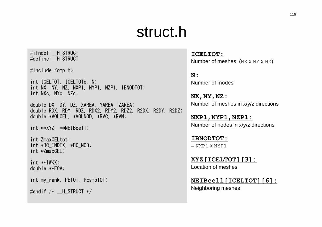
struct.h#ifndef __H_STRUCT#define __H_STRUCT
#include <omp.h>
int ICELTOT, ICELTOTp, N;int NX, NY, NZ, NXP1, NYP1, NZP1, IBNODTOT;int NXc, NYc, NZc;
double DX, DY, DZ, XAREA, YAREA, ZAREA;double RDX, RDY, RDZ, RDX2, RDY2, RDZ2, R2DX, R2DY, R2DZ;double *VOLCEL, *VOLNOD, *RVC, *RVN;
int **XYZ, **NEIBcell;
int ZmaxCELtot;int *BC_INDEX, *BC_NOD;int *ZmaxCEL;
int **IWKX;double **FCV;
int my_rank, PETOT, PEsmpTOT;
#endif /* __H_STRUCT */
ICELTOT:Number of meshes (NX x NY x NZ)
N: Number of modes
NX,NY,NZ:Number of meshes in x/y/z directions
NXP1,NYP1,NZP1:Number of nodes in x/y/z directions
IBNODTOT:= NXP1 x NYP1
XYZ[ICELTOT][3]:Location of meshes
NEIBcell[ICELTOT][6]:Neighboring meshes
120
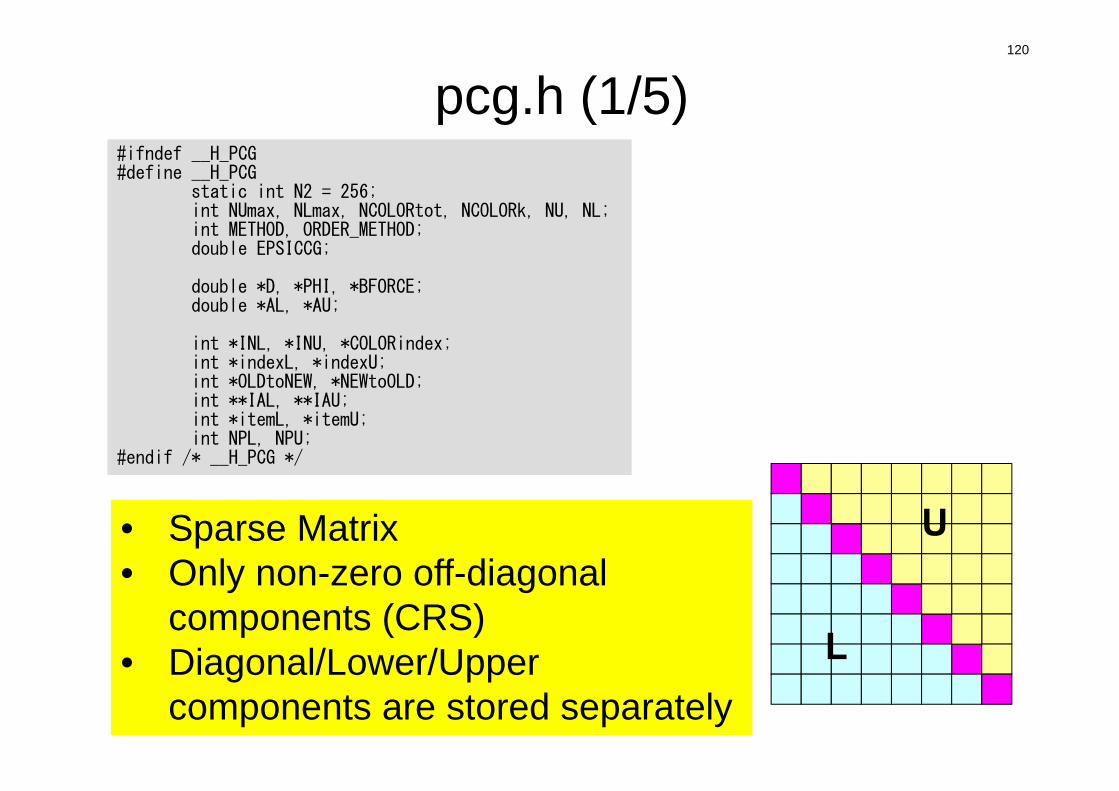
pcg.h (1/5)#ifndef __H_PCG#define __H_PCG
static int N2 = 256;int NUmax, NLmax, NCOLORtot, NCOLORk, NU, NL;int METHOD, ORDER_METHOD;double EPSICCG;
double *D, *PHI, *BFORCE;double *AL, *AU;
int *INL, *INU, *COLORindex;int *indexL, *indexU;int *OLDtoNEW, *NEWtoOLD;int **IAL, **IAU;int *itemL, *itemU;int NPL, NPU;
#endif /* __H_PCG */
• Sparse Matrix• Only non-zero off-diagonal
components (CRS)• Diagonal/Lower/Upper
components are stored separately
U
L
121
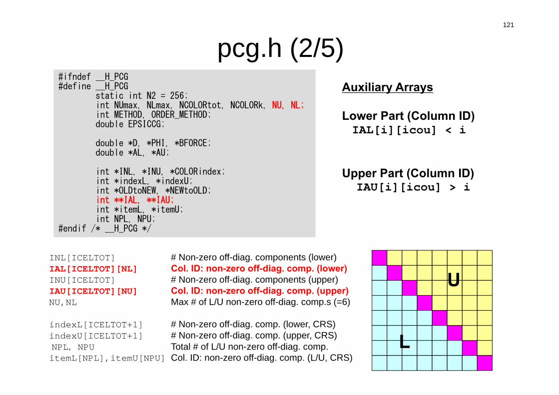
pcg.h (2/5)
INL[ICELTOT] # Non-zero off-diag. components (lower)IAL[ICELTOT][NL] Col. ID: non-zero off-diag. comp. (lower) INU[ICELTOT] # Non-zero off-diag. components (upper)IAU[ICELTOT][NU] Col. ID: non-zero off-diag. comp. (upper) NU,NL Max # of L/U non-zero off-diag. comp.s (=6)
indexL[ICELTOT+1] # Non-zero off-diag. comp. (lower, CRS)indexU[ICELTOT+1] # Non-zero off-diag. comp. (upper, CRS)NPL,NPU Total # of L/U non-zero off-diag. comp.itemL[NPL],itemU[NPU] Col. ID: non-zero off-diag. comp. (L/U, CRS)
Auxiliary Arrays
Lower Part (Column ID)IAL[i][icou] < i
Upper Part (Column ID)IAU[i][icou] > i
U
L
#ifndef __H_PCG#define __H_PCG
static int N2 = 256;int NUmax, NLmax, NCOLORtot, NCOLORk, NU, NL;int METHOD, ORDER_METHOD;double EPSICCG;
double *D, *PHI, *BFORCE;double *AL, *AU;
int *INL, *INU, *COLORindex;int *indexL, *indexU;int *OLDtoNEW, *NEWtoOLD;int **IAL, **IAU;int *itemL, *itemU;int NPL, NPU;
#endif /* __H_PCG */

122
pcg.h (3/5)
U
L
Auxiliary Arrays
Lower Part (Column ID)IAL[i][icou] < iINL[i]: Number@each row
Upper Part (Column ID)IAU[i][icou] > iINU[i]: Number@each row
INL[ICELTOT] # Non-zero off-diag. components (lower)IAL[ICELTOT][NL] Col. ID: non-zero off-diag. comp. (lower) INU[ICELTOT] # Non-zero off-diag. components (upper)IAU[ICELTOT][NU] Col. ID: non-zero off-diag. comp. (upper) NU,NL Max # of L/U non-zero off-diag. comp.s (=6)
indexL[ICELTOT+1] # Non-zero off-diag. comp. (lower, CRS)indexU[ICELTOT+1] # Non-zero off-diag. comp. (upper, CRS)NPL,NPU Total # of L/U non-zero off-diag. comp.itemL[NPL],itemU[NPU] Col. ID: non-zero off-diag. comp. (L/U, CRS)
#ifndef __H_PCG#define __H_PCG
static int N2 = 256;int NUmax, NLmax, NCOLORtot, NCOLORk, NU, NL;int METHOD, ORDER_METHOD;double EPSICCG;
double *D, *PHI, *BFORCE;double *AL, *AU;
int *INL, *INU, *COLORindex;int *indexL, *indexU;int *OLDtoNEW, *NEWtoOLD;int **IAL, **IAU;int *itemL, *itemU;int NPL, NPU;
#endif /* __H_PCG */
123
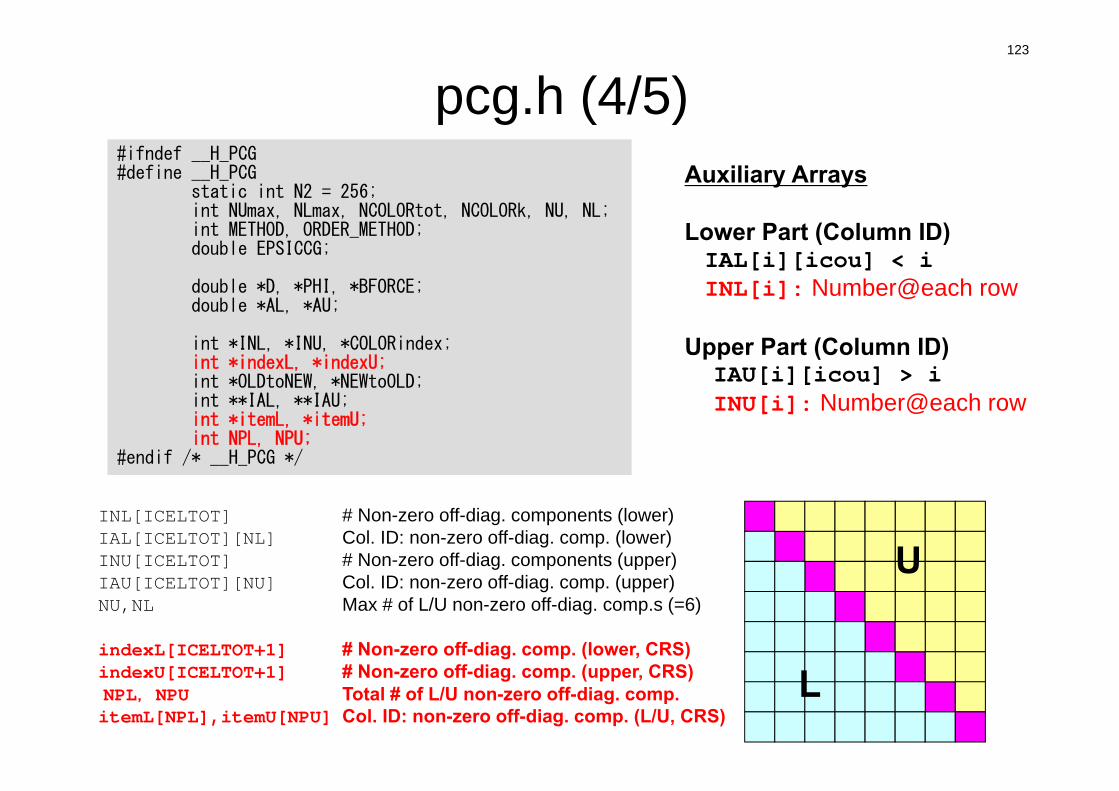
pcg.h (4/5)
U
L
Auxiliary Arrays
Lower Part (Column ID)IAL[i][icou] < iINL[i]: Number@each row
Upper Part (Column ID)IAU[i][icou] > iINU[i]: Number@each row
INL[ICELTOT] # Non-zero off-diag. components (lower)IAL[ICELTOT][NL] Col. ID: non-zero off-diag. comp. (lower) INU[ICELTOT] # Non-zero off-diag. components (upper)IAU[ICELTOT][NU] Col. ID: non-zero off-diag. comp. (upper) NU,NL Max # of L/U non-zero off-diag. comp.s (=6)
indexL[ICELTOT+1] # Non-zero off-diag. comp. (lower, CRS)indexU[ICELTOT+1] # Non-zero off-diag. comp. (upper, CRS)NPL,NPU Total # of L/U non-zero off-diag. comp.itemL[NPL],itemU[NPU] Col. ID: non-zero off-diag. comp. (L/U, CRS)
#ifndef __H_PCG#define __H_PCG
static int N2 = 256;int NUmax, NLmax, NCOLORtot, NCOLORk, NU, NL;int METHOD, ORDER_METHOD;double EPSICCG;
double *D, *PHI, *BFORCE;double *AL, *AU;
int *INL, *INU, *COLORindex;int *indexL, *indexU;int *OLDtoNEW, *NEWtoOLD;int **IAL, **IAU;int *itemL, *itemU;int NPL, NPU;
#endif /* __H_PCG */
124
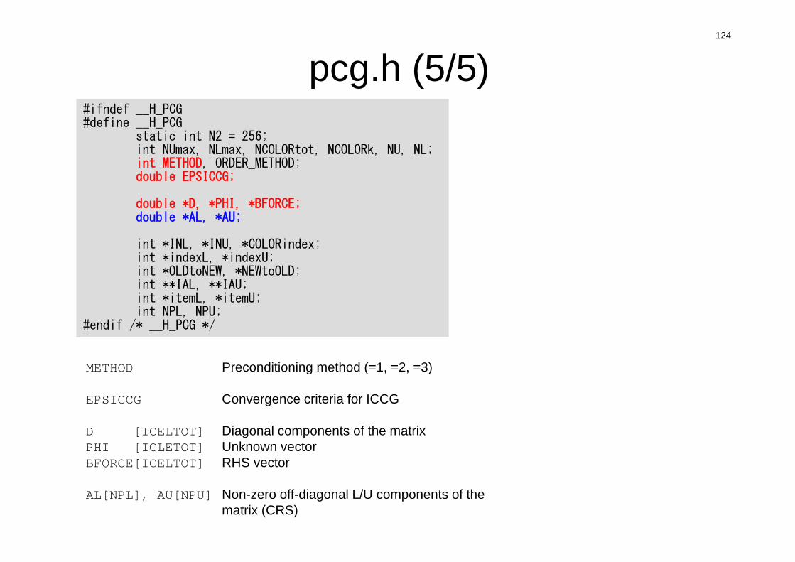
pcg.h (5/5)
METHOD Preconditioning method (=1, =2, =3)
EPSICCG Convergence criteria for ICCG
D [ICELTOT] Diagonal components of the matrixPHI [ICLETOT] Unknown vectorBFORCE[ICELTOT] RHS vector
AL[NPL], AU[NPU] Non-zero off-diagonal L/U components of the matrix (CRS)
#ifndef __H_PCG#define __H_PCG
static int N2 = 256;int NUmax, NLmax, NCOLORtot, NCOLORk, NU, NL;int METHOD, ORDER_METHOD;double EPSICCG;
double *D, *PHI, *BFORCE;double *AL, *AU;
int *INL, *INU, *COLORindex;int *indexL, *indexU;int *OLDtoNEW, *NEWtoOLD;int **IAL, **IAU;int *itemL, *itemU;int NPL, NPU;
#endif /* __H_PCG */
125
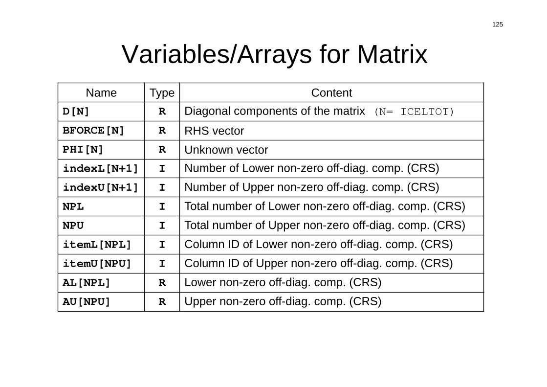
Variables/Arrays for MatrixName Type Content
D[N] R Diagonal components of the matrix (N= ICELTOT)
BFORCE[N] R RHS vectorPHI[N] R Unknown vectorindexL[N+1] I Number of Lower non-zero off-diag. comp. (CRS)indexU[N+1] I Number of Upper non-zero off-diag. comp. (CRS)NPL I Total number of Lower non-zero off-diag. comp. (CRS)NPU I Total number of Upper non-zero off-diag. comp. (CRS)itemL[NPL] I Column ID of Lower non-zero off-diag. comp. (CRS)itemU[NPU] I Column ID of Upper non-zero off-diag. comp. (CRS)AL[NPL] R Lower non-zero off-diag. comp. (CRS)AU[NPU] R Upper non-zero off-diag. comp. (CRS)
126
Variables/Arrays for MatrixAuxiliary Arrays
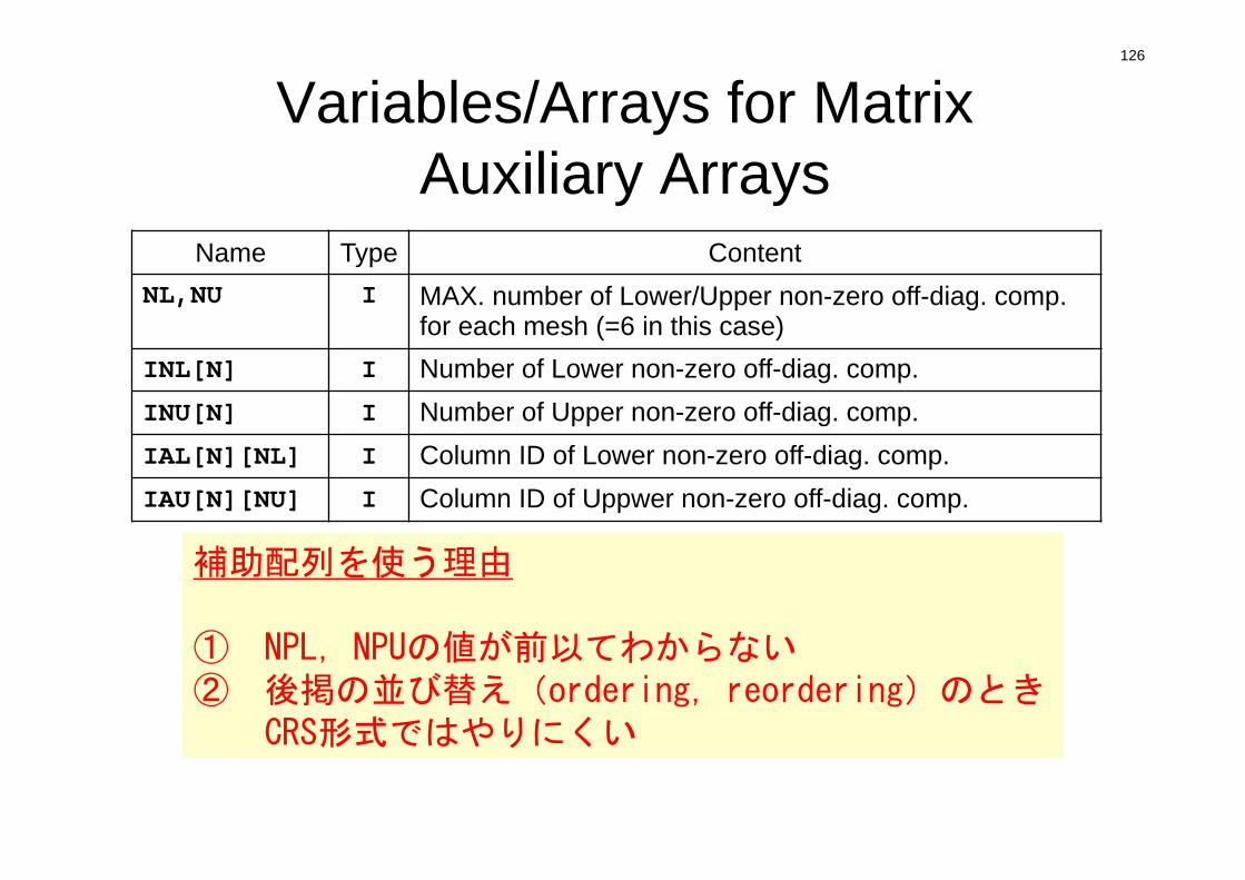
Name Type ContentNL,NU I MAX. number of Lower/Upper non-zero off-diag. comp.
for each mesh (=6 in this case) INL[N] I Number of Lower non-zero off-diag. comp.INU[N] I Number of Upper non-zero off-diag. comp.IAL[N][NL] I Column ID of Lower non-zero off-diag. comp.IAU[N][NU] I Column ID of Uppwer non-zero off-diag. comp.
補助配列を使う理由
① NPL,NPUの値が前以てわからない② 後掲の並び替え(ordering,reordering)のとき
CRS形式ではやりにくい
127
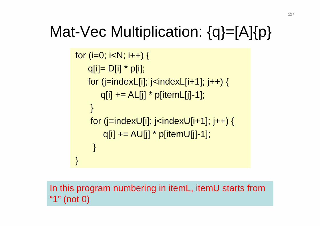
Mat-Vec Multiplication: {q}=[A]{p}for (i=0; i<N; i++) {
q[i]= D[i] * p[i];for (j=indexL[i]; j<indexL[i+1]; j++) {
q[i] += AL[j] * p[itemL[j]-1];}for (j=indexU[i]; j<indexU[i+1]; j++) {
q[i] += AU[j] * p[itemU[j]-1];}
}
In this program numbering in itemL, itemU starts from “1” (not 0)
#include <stdio.h>#include <stdlib.h>#include <string.h>#include <errno.h>
#include "struct.h"#include "pcg.h"#include "input.h“ ...
intmain(){double *WK;int NPL, NPU; ISET, ITR, IER; icel, ic0, i;double xN, xL, xU; Stime, Etime;
if(INPUT()) goto error;if(POINTER_INIT()) goto error;if(BOUNDARY_CELL()) goto error;if(CELL_METRICS()) goto error;if(POI_GEN()) goto error;
memset(PHI, 0.0, sizeof(double)*ICELTOT);ISET = 0;WK = (double *)malloc(sizeof(double)*ICELTOT);
if(METHOD==1){if(solve_ICCG(...)) goto error;} else if(METHOD==3){if(solve_PCG(...)) goto error;}
if(OUTUCD()) goto error;return 0;
error:return -1;
}
MAINメインルーチン
INPUT制御ファイル読込INPUT.DAT
POINTER_INITメッシュファイル読込
mesh.dat
BOUNDARY_CELL=0を設定する要素の探索
CELL_METRICS表面積,体積等の計算
POI_GEN行列コネクティビティ生成,各成分の計算,境界条件
SOLVER_ICCGICCG法ソルバー
METHOD=1
SOLVER_ICCG2ICCG法ソルバー
METHOD=2
SOLVER_PCGICCG法ソルバー
METHOD=3
FORM_ILU0
jkk
j
kikijij ldlal ~~~~ 1
1
128
Structure of the Program
main control info.
mesh info.
boundary meshes
area/volume
matrix
ICCG: METH=1
ICCG: METH=2
PCG: METH=3
129
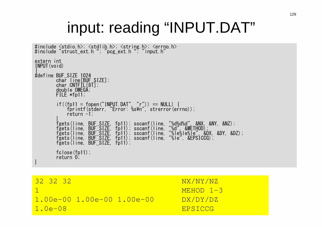
input: reading “INPUT.DAT”#include <stdio.h>; <stdlib.h>; <string.h>; <errno.h>#include "struct_ext.h“; "pcg_ext.h“; "input.h"
extern intINPUT(void){#define BUF_SIZE 1024
char line[BUF_SIZE];char CNTFIL[81];double OMEGA;FILE *fp11;
if((fp11 = fopen("INPUT.DAT", "r")) == NULL) {fprintf(stderr, "Error: %s¥n", strerror(errno));return -1;
}fgets(line, BUF_SIZE, fp11); sscanf(line, "%d%d%d", &NX, &NY, &NZ);fgets(line, BUF_SIZE, fp11); sscanf(line, "%d", &METHOD);fgets(line, BUF_SIZE, fp11); sscanf(line, "%le%le%le", &DX, &DY, &DZ);fgets(line, BUF_SIZE, fp11); sscanf(line, "%le", &EPSICCG);fgets(line, BUF_SIZE, fp11);
fclose(fp11);return 0;
}
32 32 32 NX/NY/NZ1 MEHOD 1-31.00e-00 1.00e-00 1.00e-00 DX/DY/DZ1.0e-08 EPSICCG
130
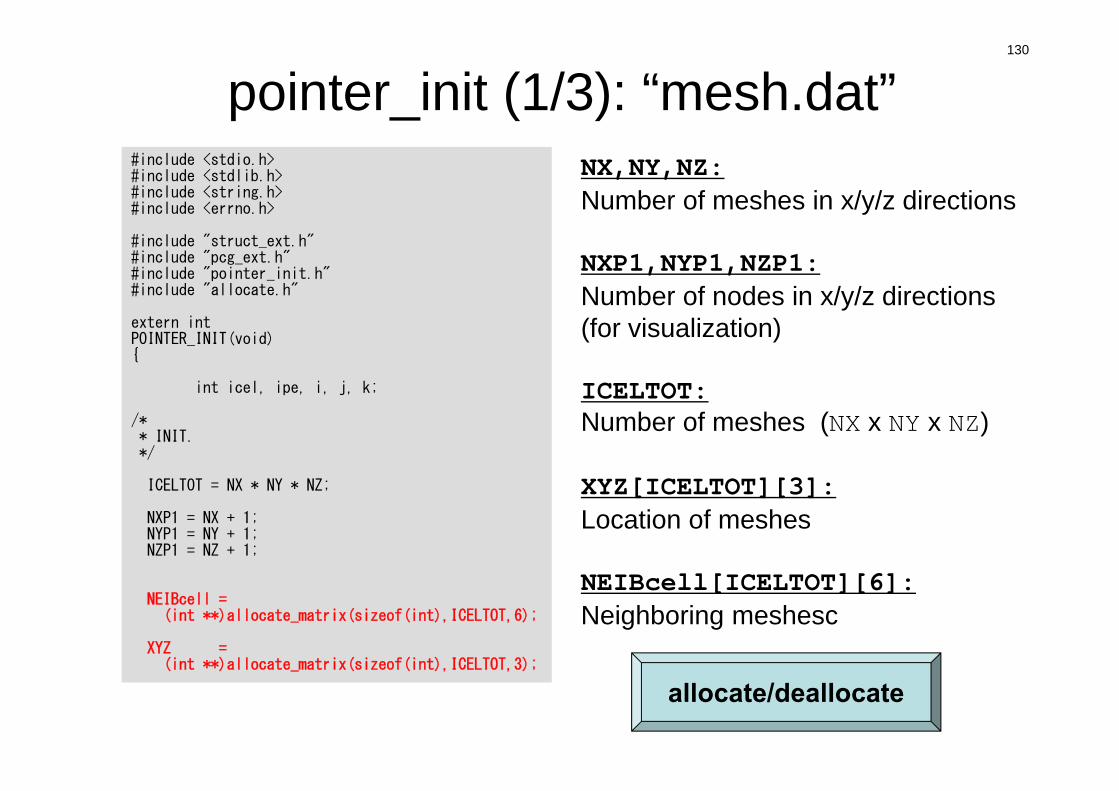
pointer_init (1/3): “mesh.dat”#include <stdio.h>#include <stdlib.h>#include <string.h>#include <errno.h>
#include "struct_ext.h"#include "pcg_ext.h"#include "pointer_init.h"#include "allocate.h"
extern intPOINTER_INIT(void){
int icel, ipe, i, j, k;
/** INIT.*/
ICELTOT = NX * NY * NZ;
NXP1 = NX + 1;NYP1 = NY + 1;NZP1 = NZ + 1;
NEIBcell = (int **)allocate_matrix(sizeof(int),ICELTOT,6);
XYZ = (int **)allocate_matrix(sizeof(int),ICELTOT,3);
NX,NY,NZ:Number of meshes in x/y/z directions
NXP1,NYP1,NZP1:Number of nodes in x/y/z directions (for visualization)
ICELTOT:Number of meshes (NX x NY x NZ)
XYZ[ICELTOT][3]:Location of meshes
NEIBcell[ICELTOT][6]:Neighboring meshesc
allocate/deallocate
131
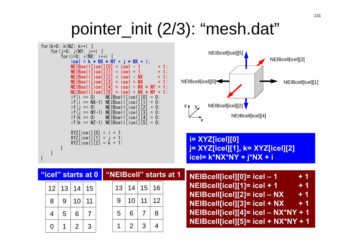
pointer_init (2/3): “mesh.dat”for(k=0; k<NZ; k++) {
for(j=0; j<NY; j++) {for(i=0; i<NX; i++) {
icel = k * NX * NY + j * NX + i;NEIBcell[icel][0] = icel - 1 + 1;NEIBcell[icel][1] = icel + 1 + 1;NEIBcell[icel][2] = icel - NX + 1;NEIBcell[icel][3] = icel + NX + 1;NEIBcell[icel][4] = icel - NX * NY + 1;NEIBcell[icel][5] = icel + NX * NY + 1;if(i == 0) NEIBcell[icel][0] = 0;if(i == NX-1) NEIBcell[icel][1] = 0;if(j == 0) NEIBcell[icel][2] = 0;if(j == NY-1) NEIBcell[icel][3] = 0;if(k == 0) NEIBcell[icel][4] = 0;if(k == NZ-1) NEIBcell[icel][5] = 0;
XYZ[icel][0] = i + 1;XYZ[icel][1] = j + 1;XYZ[icel][2] = k + 1;
}}
}
i= XYZ[icel][0]j= XYZ[icel][1], k= XYZ[icel][2]icel= k*NX*NY + j*NX + i
NEIBcell[icel][0]= icel – 1 + 1 NEIBcell[icel][1]= icel + 1 + 1NEIBcell[icel][2]= icel – NX + 1NEIBcell[icel][3]= icel + NX + 1NEIBcell[icel][4]= icel – NX*NY + 1NEIBcell[icel][5]= icel + NX*NY + 1
NEIBcell(icel,2)NEIBcell(icel,1)
NEIBcell(icel,3)
NEIBcell(icel,5)
NEIBcell(icel,4)NEIBcell(icel,6)
NEIBcell(icel,2)NEIBcell(icel,1)
NEIBcell(icel,3)
NEIBcell(icel,5)
NEIBcell(icel,4)NEIBcell(icel,6)
x
yz
x
yz
NEIBcell[icel][3]
NEIBcell[icel][1]NEIBcell[icel][0]
NEIBcell[icel][2]
NEIBcell[icel][4]
NEIBcell[icel][5]
1 2 3 4
5 6 7 8
9 10 11 12
13 14 15 16
0 1 2 3
4 5 6 7
8 9 10 11
12 13 14 15
“icel” starts at 0 “NEIBcell” starts at 1
132
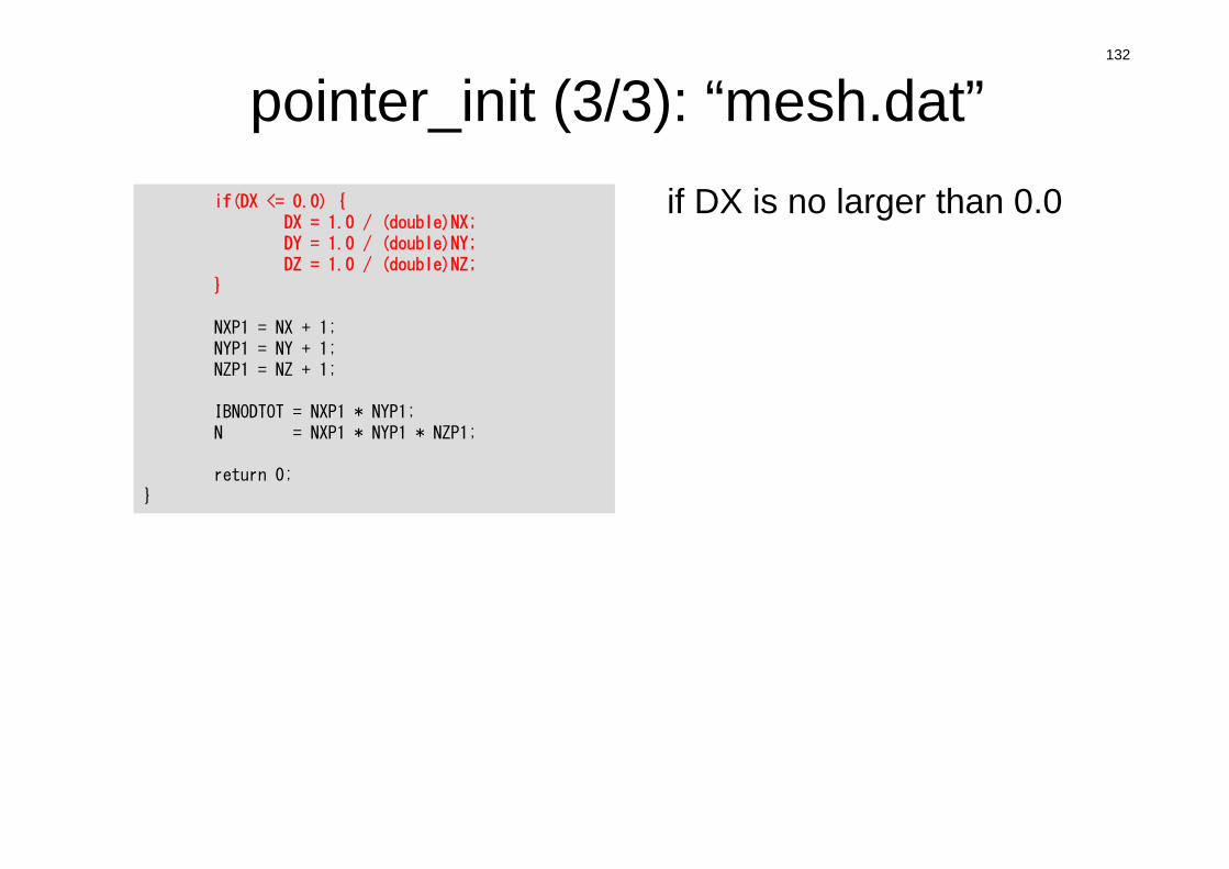
pointer_init (3/3): “mesh.dat”if DX is no larger than 0.0if(DX <= 0.0) {
DX = 1.0 / (double)NX;DY = 1.0 / (double)NY;DZ = 1.0 / (double)NZ;
}
NXP1 = NX + 1;NYP1 = NY + 1;NZP1 = NZ + 1;
IBNODTOT = NXP1 * NYP1;N = NXP1 * NYP1 * NZP1;
return 0;}
133
pointer_init (3/3): “mesh.dat”
1 2
4 3
5 6
7 8
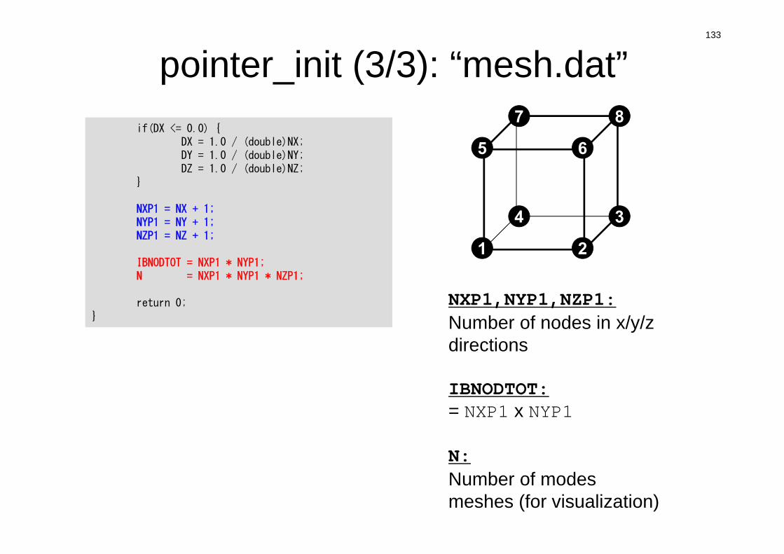
NXP1,NYP1,NZP1:Number of nodes in x/y/z directions
IBNODTOT:= NXP1 x NYP1
N: Number of modesmeshes (for visualization)
if(DX <= 0.0) {DX = 1.0 / (double)NX;DY = 1.0 / (double)NY;DZ = 1.0 / (double)NZ;
}
NXP1 = NX + 1;NYP1 = NY + 1;NZP1 = NZ + 1;
IBNODTOT = NXP1 * NYP1;N = NXP1 * NYP1 * NZP1;
return 0;}
134
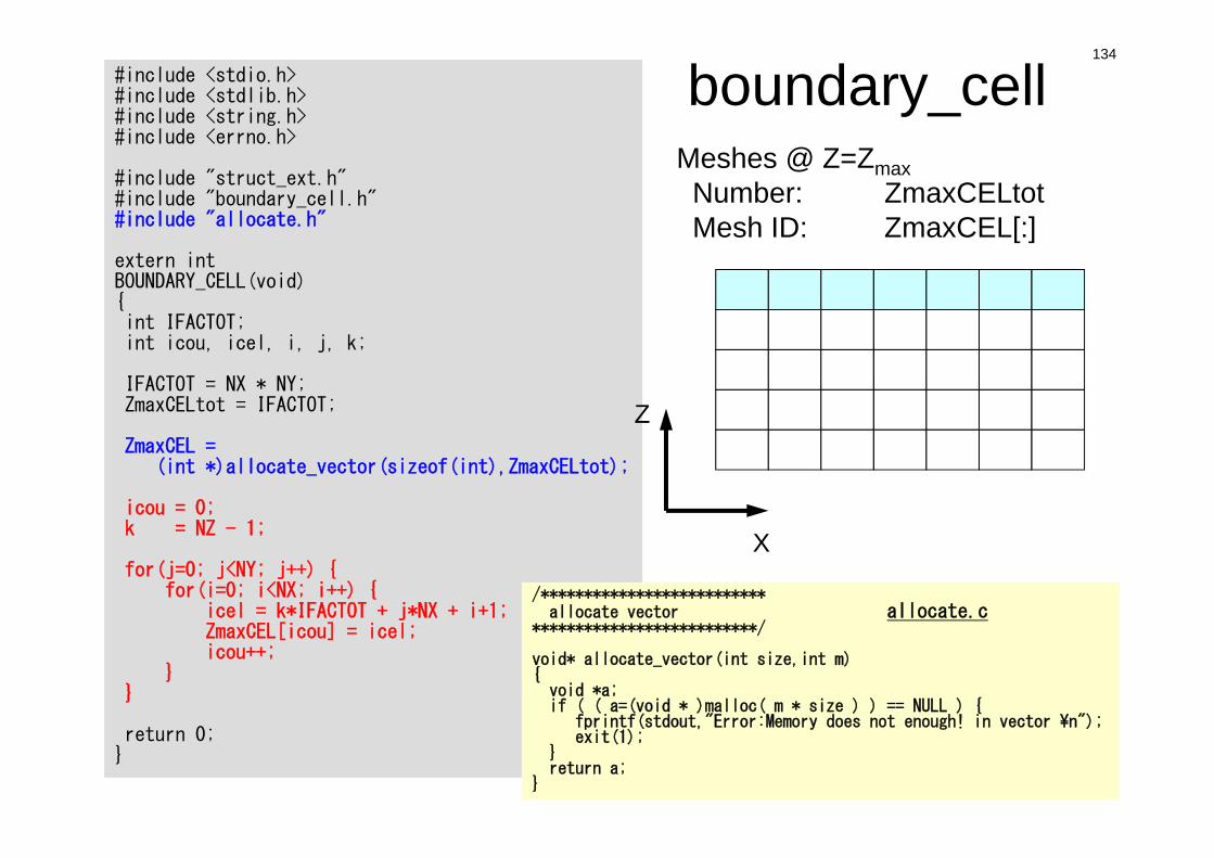
boundary_cell#include <stdio.h>#include <stdlib.h>#include <string.h>#include <errno.h>
#include "struct_ext.h"#include "boundary_cell.h"#include "allocate.h"
extern intBOUNDARY_CELL(void){int IFACTOT;int icou, icel, i, j, k;
IFACTOT = NX * NY;ZmaxCELtot = IFACTOT;
ZmaxCEL = (int *)allocate_vector(sizeof(int),ZmaxCELtot);
icou = 0;k = NZ - 1;
for(j=0; j<NY; j++) {for(i=0; i<NX; i++) {
icel = k*IFACTOT + j*NX + i+1;ZmaxCEL[icou] = icel;icou++;
}}
return 0;}
Meshes @ Z=ZmaxNumber: ZmaxCELtotMesh ID: ZmaxCEL[:]
X
Z
/**************************allocate vector allocate.c
**************************/
void* allocate_vector(int size,int m){void *a;if ( ( a=(void * )malloc( m * size ) ) == NULL ) {
fprintf(stdout,"Error:Memory does not enough! in vector ¥n");exit(1);
}return a;
}
135
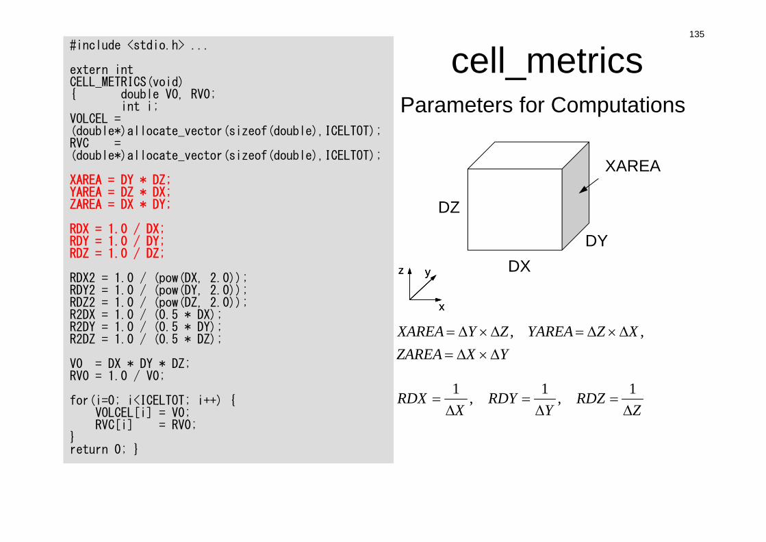
cell_metrics#include <stdio.h> ...
extern intCELL_METRICS(void){ double V0, RV0;
int i;VOLCEL = (double*)allocate_vector(sizeof(double),ICELTOT);RVC = (double*)allocate_vector(sizeof(double),ICELTOT);
XAREA = DY * DZ;YAREA = DZ * DX;ZAREA = DX * DY;
RDX = 1.0 / DX;RDY = 1.0 / DY;RDZ = 1.0 / DZ;
RDX2 = 1.0 / (pow(DX, 2.0));RDY2 = 1.0 / (pow(DY, 2.0));RDZ2 = 1.0 / (pow(DZ, 2.0));R2DX = 1.0 / (0.5 * DX);R2DY = 1.0 / (0.5 * DY);R2DZ = 1.0 / (0.5 * DZ);
V0 = DX * DY * DZ;RV0 = 1.0 / V0;
for(i=0; i<ICELTOT; i++) {VOLCEL[i] = V0;RVC[i] = RV0;
}return 0; }
Parameters for Computations
x
yz
x
yz DXDY
DZ
XAREA
YXZAREAXZYAREAZYXAREA
,,
ZRDZ
YRDY
XRDX
1,1,1
136
cell_metrics
x
yz
x
yz DXDY
DZ
XAREA
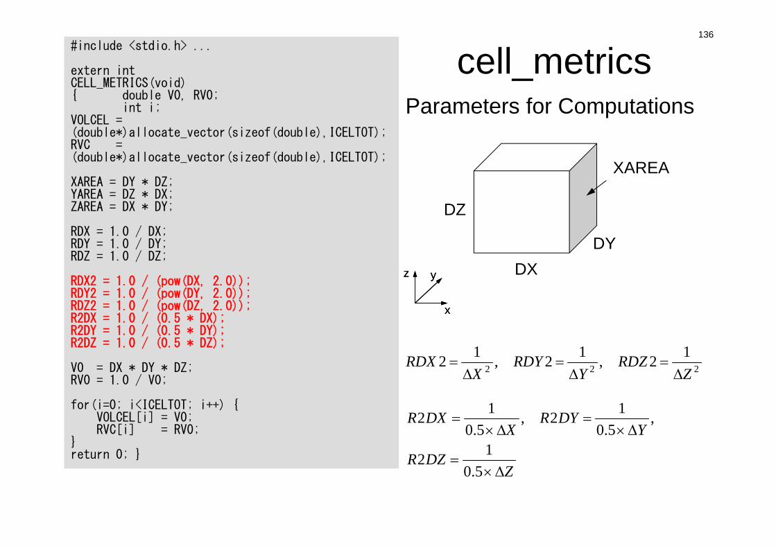
22212,12,12Z
RDZY
RDYX
RDX
ZDZR
YDYR
XDXR
5.012
,5.0
12,5.0
12
Parameters for Computations
#include <stdio.h> ...
extern intCELL_METRICS(void){ double V0, RV0;
int i;VOLCEL = (double*)allocate_vector(sizeof(double),ICELTOT);RVC = (double*)allocate_vector(sizeof(double),ICELTOT);
XAREA = DY * DZ;YAREA = DZ * DX;ZAREA = DX * DY;
RDX = 1.0 / DX;RDY = 1.0 / DY;RDZ = 1.0 / DZ;
RDX2 = 1.0 / (pow(DX, 2.0));RDY2 = 1.0 / (pow(DY, 2.0));RDZ2 = 1.0 / (pow(DZ, 2.0));R2DX = 1.0 / (0.5 * DX);R2DY = 1.0 / (0.5 * DY);R2DZ = 1.0 / (0.5 * DZ);
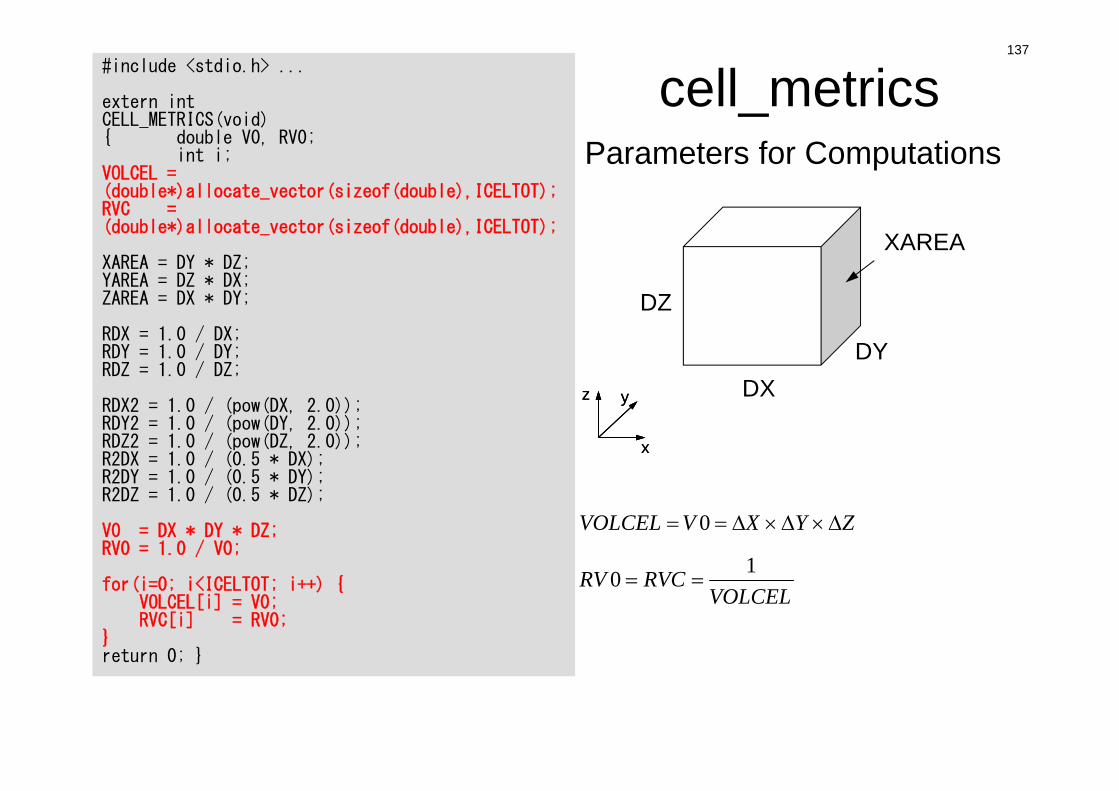
V0 = DX * DY * DZ;RV0 = 1.0 / V0;
for(i=0; i<ICELTOT; i++) {VOLCEL[i] = V0;RVC[i] = RV0;
}return 0; }
137
cell_metrics
x
yz
x
yz DXDY
DZ
XAREA
ZYXVVOLCEL 0
VOLCELRVCRV 10
Parameters for Computations
#include <stdio.h> ...
extern intCELL_METRICS(void){ double V0, RV0;
int i;VOLCEL = (double*)allocate_vector(sizeof(double),ICELTOT);RVC = (double*)allocate_vector(sizeof(double),ICELTOT);
XAREA = DY * DZ;YAREA = DZ * DX;ZAREA = DX * DY;
RDX = 1.0 / DX;RDY = 1.0 / DY;RDZ = 1.0 / DZ;
RDX2 = 1.0 / (pow(DX, 2.0));RDY2 = 1.0 / (pow(DY, 2.0));RDZ2 = 1.0 / (pow(DZ, 2.0));R2DX = 1.0 / (0.5 * DX);R2DY = 1.0 / (0.5 * DY);R2DZ = 1.0 / (0.5 * DZ);
V0 = DX * DY * DZ;RV0 = 1.0 / V0;
for(i=0; i<ICELTOT; i++) {VOLCEL[i] = V0;RVC[i] = RV0;
}return 0; }
#include <stdio.h>#include <stdlib.h>#include <string.h>#include <errno.h>
#include "struct.h"#include "pcg.h"#include "input.h“ ...
intmain(){double *WK;int NPL, NPU; ISET, ITR, IER; icel, ic0, i;double xN, xL, xU; Stime, Etime;
if(INPUT()) goto error;if(POINTER_INIT()) goto error;if(BOUNDARY_CELL()) goto error;if(CELL_METRICS()) goto error;if(POI_GEN()) goto error;
memset(PHI, 0.0, sizeof(double)*ICELTOT);ISET = 0;WK = (double *)malloc(sizeof(double)*ICELTOT);
if(METHOD==1){if(solve_ICCG(...)) goto error;} else if(METHOD==3){if(solve_PCG(...)) goto error;}
if(OUTUCD()) goto error;return 0;
error:return -1;
}
138
Structure of the ProgramMAIN
メインルーチン
INPUT制御ファイル読込INPUT.DAT
POINTER_INITメッシュファイル読込
mesh.dat
BOUNDARY_CELL=0を設定する要素の探索
CELL_METRICS表面積,体積等の計算
POI_GEN行列コネクティビティ生成,各成分の計算,境界条件
SOLVER_ICCGICCG法ソルバー
METHOD=1
SOLVER_ICCG2ICCG法ソルバー
METHOD=2
SOLVER_PCGICCG法ソルバー
METHOD=3
FORM_ILU0
jkk
j
kikijij ldlal ~~~~ 1
1
main control info.
mesh info.
boundary meshes
area/volume
matrix
ICCG: METH=1
ICCG: METH=2
PCG: METH=3
139
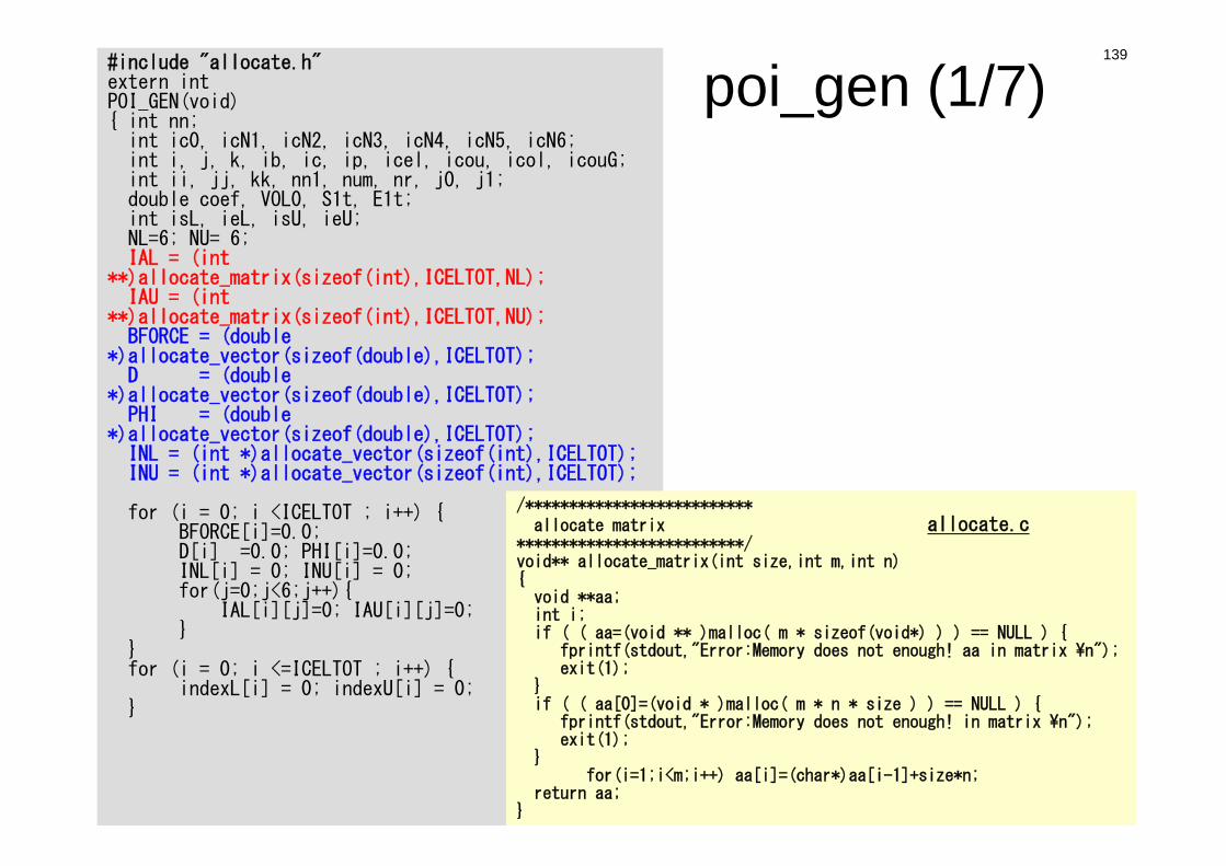
poi_gen (1/7)#include "allocate.h"extern intPOI_GEN(void){ int nn;
int ic0, icN1, icN2, icN3, icN4, icN5, icN6;int i, j, k, ib, ic, ip, icel, icou, icol, icouG;int ii, jj, kk, nn1, num, nr, j0, j1;double coef, VOL0, S1t, E1t;int isL, ieL, isU, ieU;NL=6; NU= 6;IAL = (int
**)allocate_matrix(sizeof(int),ICELTOT,NL);IAU = (int
**)allocate_matrix(sizeof(int),ICELTOT,NU);BFORCE = (double
*)allocate_vector(sizeof(double),ICELTOT);D = (double
*)allocate_vector(sizeof(double),ICELTOT);PHI = (double
*)allocate_vector(sizeof(double),ICELTOT);INL = (int *)allocate_vector(sizeof(int),ICELTOT);INU = (int *)allocate_vector(sizeof(int),ICELTOT);
for (i = 0; i <ICELTOT ; i++) {BFORCE[i]=0.0;D[i] =0.0; PHI[i]=0.0;INL[i] = 0; INU[i] = 0;for(j=0;j<6;j++){
IAL[i][j]=0; IAU[i][j]=0;}
}for (i = 0; i <=ICELTOT ; i++) {
indexL[i] = 0; indexU[i] = 0;}
/**************************allocate matrix allocate.c
**************************/void** allocate_matrix(int size,int m,int n){void **aa;int i;if ( ( aa=(void ** )malloc( m * sizeof(void*) ) ) == NULL ) {
fprintf(stdout,"Error:Memory does not enough! aa in matrix ¥n");exit(1);
}if ( ( aa[0]=(void * )malloc( m * n * size ) ) == NULL ) {
fprintf(stdout,"Error:Memory does not enough! in matrix ¥n");exit(1);
}for(i=1;i<m;i++) aa[i]=(char*)aa[i-1]+size*n;
return aa;}
140
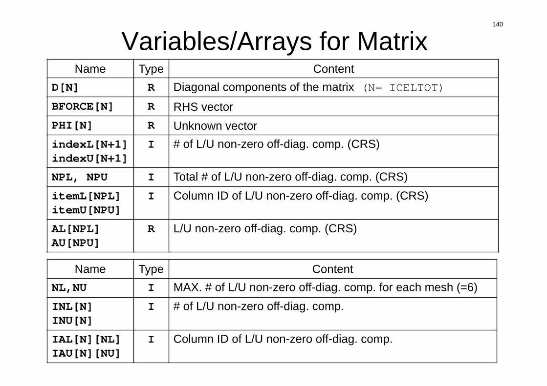
Variables/Arrays for MatrixName Type Content
D[N] R Diagonal components of the matrix (N= ICELTOT)
BFORCE[N] R RHS vectorPHI[N] R Unknown vectorindexL[N+1] indexU[N+1]
I # of L/U non-zero off-diag. comp. (CRS)
NPL, NPU I Total # of L/U non-zero off-diag. comp. (CRS)itemL[NPL] itemU[NPU]
I Column ID of L/U non-zero off-diag. comp. (CRS)
AL[NPL] AU[NPU]
R L/U non-zero off-diag. comp. (CRS)
Name Type ContentNL,NU I MAX. # of L/U non-zero off-diag. comp. for each mesh (=6) INL[N]INU[N]
I # of L/U non-zero off-diag. comp.
IAL[N][NL]IAU[N][NU]
I Column ID of L/U non-zero off-diag. comp.
141
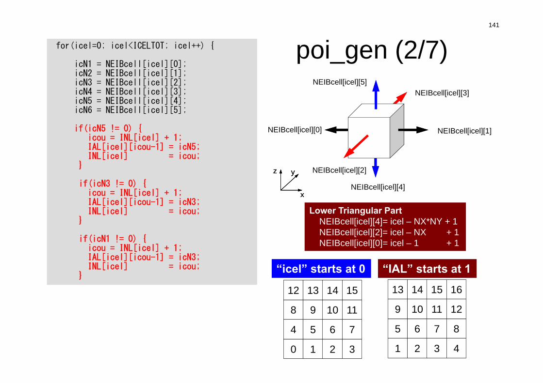
poi_gen (2/7)
Lower Triangular PartNEIBcell[icel][4]= icel – NX*NY + 1NEIBcell[icel][2]= icel – NX + 1NEIBcell[icel][0]= icel – 1 + 1
for(icel=0; icel<ICELTOT; icel++) {
icN1 = NEIBcell[icel][0];icN2 = NEIBcell[icel][1];icN3 = NEIBcell[icel][2];icN4 = NEIBcell[icel][3];icN5 = NEIBcell[icel][4];icN6 = NEIBcell[icel][5];
if(icN5 != 0) {icou = INL[icel] + 1;IAL[icel][icou-1] = icN5;INL[icel] = icou;
}
if(icN3 != 0) {icou = INL[icel] + 1;IAL[icel][icou-1] = icN3;INL[icel] = icou;
}
if(icN1 != 0) {icou = INL[icel] + 1;IAL[icel][icou-1] = icN3;INL[icel] = icou;
}
NEIBcell(icel,2)NEIBcell(icel,1)
NEIBcell(icel,3)
NEIBcell(icel,5)
NEIBcell(icel,4)NEIBcell(icel,6)
NEIBcell(icel,2)NEIBcell(icel,1)
NEIBcell(icel,3)
NEIBcell(icel,5)
NEIBcell(icel,4)NEIBcell(icel,6)
x
yz
x
yz
NEIBcell[icel][3]
NEIBcell[icel][1]NEIBcell[icel][0]
NEIBcell[icel][2]
NEIBcell[icel][4]
NEIBcell[icel][5]
1 2 3 4
5 6 7 8
9 10 11 12
13 14 15 16
0 1 2 3
4 5 6 7
8 9 10 11
12 13 14 15
“icel” starts at 0 “IAL” starts at 1
142
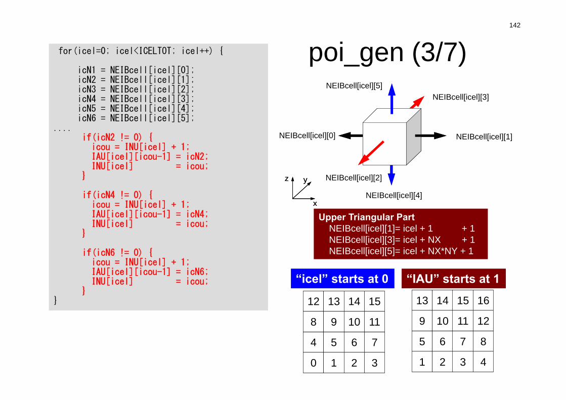
poi_gen (3/7)
Upper Triangular PartNEIBcell[icel][1]= icel + 1 + 1NEIBcell[icel][3]= icel + NX + 1NEIBcell[icel][5]= icel + NX*NY + 1
NEIBcell(icel,2)NEIBcell(icel,1)
NEIBcell(icel,3)
NEIBcell(icel,5)
NEIBcell(icel,4)NEIBcell(icel,6)
NEIBcell(icel,2)NEIBcell(icel,1)
NEIBcell(icel,3)
NEIBcell(icel,5)
NEIBcell(icel,4)NEIBcell(icel,6)
x
yz
x
yz
NEIBcell[icel][3]
NEIBcell[icel][1]NEIBcell[icel][0]
NEIBcell[icel][2]
NEIBcell[icel][4]
NEIBcell[icel][5]
1 2 3 4
5 6 7 8
9 10 11 12
13 14 15 16
0 1 2 3
4 5 6 7
8 9 10 11
12 13 14 15
“icel” starts at 0 “IAU” starts at 1
for(icel=0; icel<ICELTOT; icel++) {
icN1 = NEIBcell[icel][0];icN2 = NEIBcell[icel][1];icN3 = NEIBcell[icel][2];icN4 = NEIBcell[icel][3];icN5 = NEIBcell[icel][4];icN6 = NEIBcell[icel][5];
....if(icN2 != 0) {
icou = INU[icel] + 1;IAU[icel][icou-1] = icN2;INU[icel] = icou;
}
if(icN4 != 0) {icou = INU[icel] + 1;IAU[icel][icou-1] = icN4;INU[icel] = icou;
}
if(icN6 != 0) {icou = INU[icel] + 1;IAU[icel][icou-1] = icN6;INU[icel] = icou;
}}
143
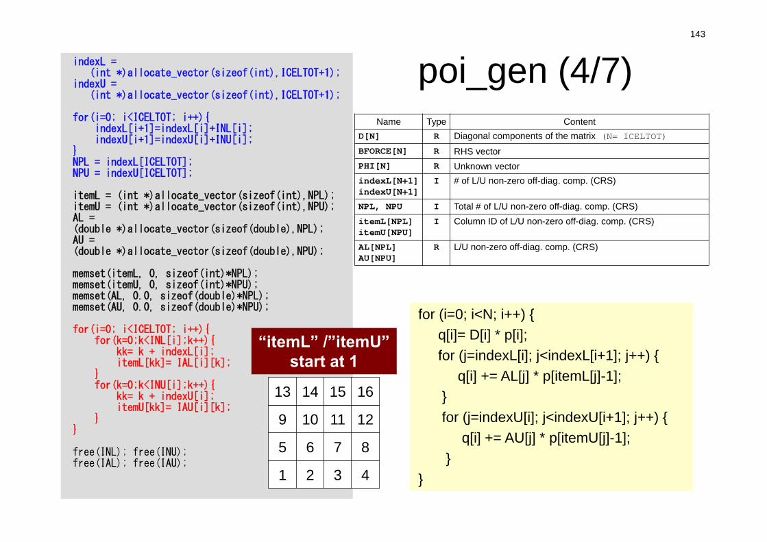
poi_gen (4/7)indexL = (int *)allocate_vector(sizeof(int),ICELTOT+1);
indexU = (int *)allocate_vector(sizeof(int),ICELTOT+1);
for(i=0; i<ICELTOT; i++){indexL[i+1]=indexL[i]+INL[i];indexU[i+1]=indexU[i]+INU[i];
}NPL = indexL[ICELTOT];NPU = indexU[ICELTOT];
itemL = (int *)allocate_vector(sizeof(int),NPL);itemU = (int *)allocate_vector(sizeof(int),NPU);AL = (double *)allocate_vector(sizeof(double),NPL);AU = (double *)allocate_vector(sizeof(double),NPU);
memset(itemL, 0, sizeof(int)*NPL);memset(itemU, 0, sizeof(int)*NPU);memset(AL, 0.0, sizeof(double)*NPL);memset(AU, 0.0, sizeof(double)*NPU);
for(i=0; i<ICELTOT; i++){for(k=0;k<INL[i];k++){
kk= k + indexL[i];itemL[kk]= IAL[i][k];
}for(k=0;k<INU[i];k++){
kk= k + indexU[i];itemU[kk]= IAU[i][k];
}}
free(INL); free(INU);free(IAL); free(IAU);
Name Type ContentD[N] R Diagonal components of the matrix (N= ICELTOT)
BFORCE[N] R RHS vectorPHI[N] R Unknown vectorindexL[N+1] indexU[N+1]
I # of L/U non-zero off-diag. comp. (CRS)
NPL, NPU I Total # of L/U non-zero off-diag. comp. (CRS)itemL[NPL] itemU[NPU]
I Column ID of L/U non-zero off-diag. comp. (CRS)
AL[NPL] AU[NPU]
R L/U non-zero off-diag. comp. (CRS)
for (i=0; i<N; i++) {q[i]= D[i] * p[i];for (j=indexL[i]; j<indexL[i+1]; j++) {
q[i] += AL[j] * p[itemL[j]-1];}for (j=indexU[i]; j<indexU[i+1]; j++) {
q[i] += AU[j] * p[itemU[j]-1];}
}1 2 3 4
5 6 7 8
9 10 11 12
13 14 15 16
“itemL” /”itemU”start at 1

144
Finite Volume Method (FVM)Conservation of Fluxes through Surfaces
i
Sia
Sib
Sic
dia dib
dic
ab
c
dbi
dai
dci
0 ii
kik
kiik
ik QVdd
S
Vi : VolumeS : Surface Areadij : Distance between
Cell-Center & Surface
Q : Volume Flux
Diffusion:Interaction with Neighbors
Volume Flux
die
145
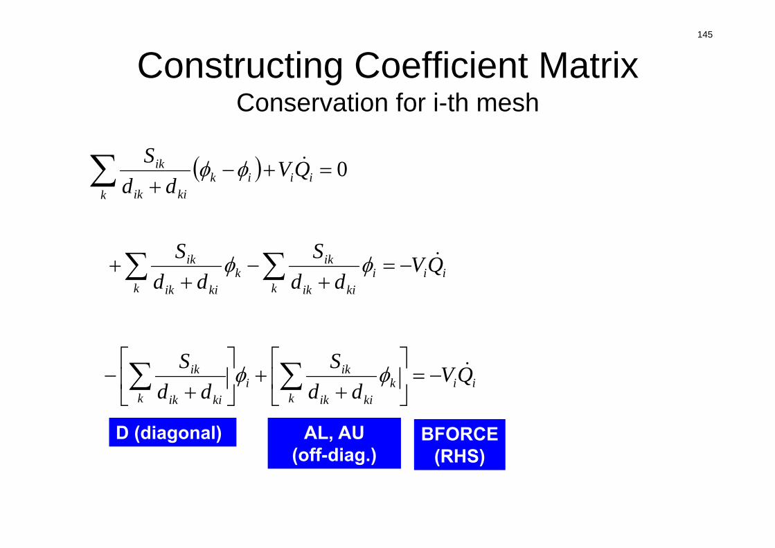
Constructing Coefficient MatrixConservation for i-th mesh
0 ii
kik
kiik
ik QVdd
S
iik
ikiik
ik
kk
kiik
ik QVdd
Sdd
S
iik
kkiik
iki
k kiik
ik QVdd
Sdd
S
D (diagonal) AL, AU(off-diag.)
BFORCE(RHS)
146
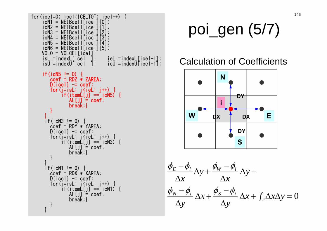
poi_gen (5/7)for(icel=0; icel<ICELTOT; icel++) {
icN1 = NEIBcell[icel][0];icN2 = NEIBcell[icel][1];icN3 = NEIBcell[icel][2];icN4 = NEIBcell[icel][3];icN5 = NEIBcell[icel][4];icN6 = NEIBcell[icel][5];VOL0 = VOLCEL[icel];isL =indexL[icel ]; ieL =indexL[icel+1];isU =indexU[icel ]; ieU =indexU[icel+1];
if(icN5 != 0) {coef = RDZ * ZAREA;D[icel] -= coef;for(j=isL; j<ieL; j++) {
if(itemL[j] == icN5) {AL[j] = coef;break;}
}}if(icN3 != 0) {coef = RDY * YAREA;D[icel] -= coef;for(j=isL; j<ieL; j++) {
if(itemL[j] == icN3) {AL[j] = coef;break;}
}} if(icN1 != 0) {coef = RDX * XAREA;D[icel] -= coef;for(j=isL; j<ieL; j++) {
if(itemL[j] == icN1) {AL[j] = coef;break;}
}}
Calculation of Coefficients
DX DX
DY
DY
0
yxfxy
xy
yx
yx
ciSiN
iWiE
i
W E
S
N
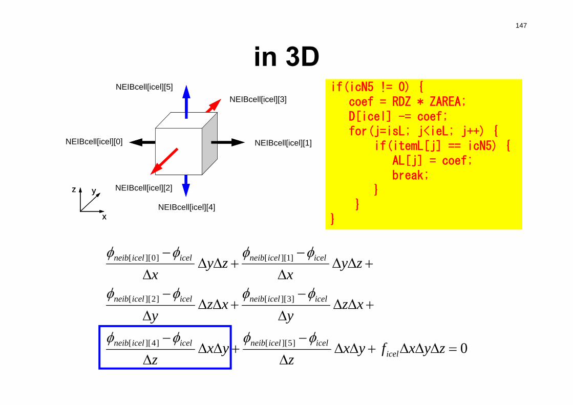
147
in 3D
0
]5][[]4][[
]3][[]2][[
]1][[]0][[
zyxfyxz
yxz
xzy
xzy
zyx
zyx
icelicelicelneibicelicelneib
icelicelneibicelicelneib
icelicelneibicelicelneib
NEIBcell(icel,2)NEIBcell(icel,1)
NEIBcell(icel,3)
NEIBcell(icel,5)
NEIBcell(icel,4)NEIBcell(icel,6)
NEIBcell(icel,2)NEIBcell(icel,1)
NEIBcell(icel,3)
NEIBcell(icel,5)
NEIBcell(icel,4)NEIBcell(icel,6)
x
yz
x
yz
NEIBcell[icel][3]
NEIBcell[icel][1]NEIBcell[icel][0]
NEIBcell[icel][2]
NEIBcell[icel][4]
NEIBcell[icel][5] if(icN5 != 0) {coef = RDZ * ZAREA;D[icel] -= coef;for(j=isL; j<ieL; j++) {
if(itemL[j] == icN5) {AL[j] = coef;break;
}}
}
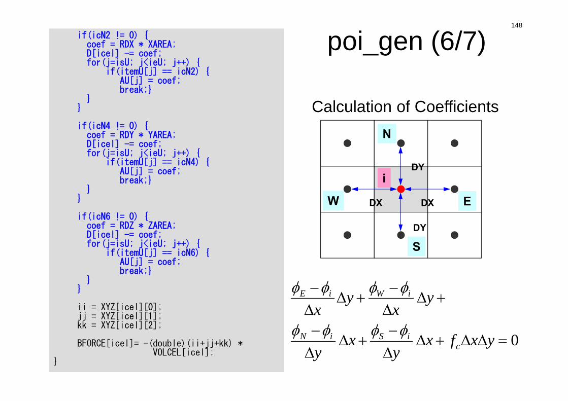
148
poi_gen (6/7)if(icN2 != 0) {coef = RDX * XAREA;D[icel] -= coef;for(j=isU; j<ieU; j++) {
if(itemU[j] == icN2) {AU[j] = coef;break;}
}}
if(icN4 != 0) {coef = RDY * YAREA;D[icel] -= coef;for(j=isU; j<ieU; j++) {
if(itemU[j] == icN4) {AU[j] = coef;break;}
}}
if(icN6 != 0) {coef = RDZ * ZAREA;D[icel] -= coef;for(j=isU; j<ieU; j++) {
if(itemU[j] == icN6) {AU[j] = coef;break;}
}}
ii = XYZ[icel][0];jj = XYZ[icel][1];kk = XYZ[icel][2];
BFORCE[icel]= -(double)(ii+jj+kk) *VOLCEL[icel];
}
DX DX
DY
DY
0
yxfxy
xy
yx
yx
ciSiN
iWiE
i
W E
S
N
Calculation of Coefficients
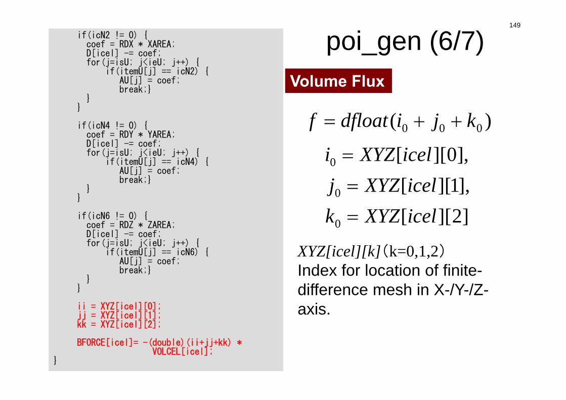
149
poi_gen (6/7)Volume Flux
)( 000 kjidfloatf
]2][[],1][[],0][[
0
0
0
icelXYZkicelXYZjicelXYZi
XYZ[icel][k](k=0,1,2)Index for location of finite-difference mesh in X-/Y-/Z-axis.
if(icN2 != 0) {coef = RDX * XAREA;D[icel] -= coef;for(j=isU; j<ieU; j++) {
if(itemU[j] == icN2) {AU[j] = coef;break;}
}}
if(icN4 != 0) {coef = RDY * YAREA;D[icel] -= coef;for(j=isU; j<ieU; j++) {
if(itemU[j] == icN4) {AU[j] = coef;break;}
}}
if(icN6 != 0) {coef = RDZ * ZAREA;D[icel] -= coef;for(j=isU; j<ieU; j++) {
if(itemU[j] == icN6) {AU[j] = coef;break;}
}}
ii = XYZ[icel][0];jj = XYZ[icel][1];kk = XYZ[icel][2];
BFORCE[icel]= -(double)(ii+jj+kk) *VOLCEL[icel];
}
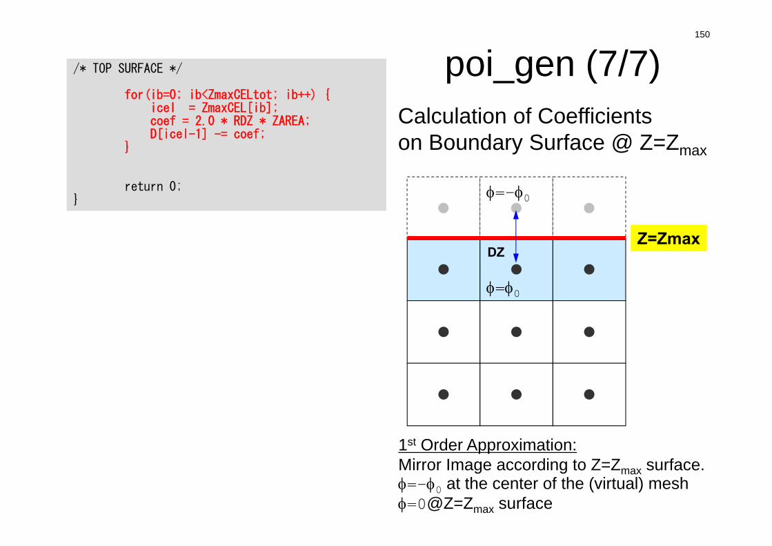
150
poi_gen (7/7)
DZZ=Zmax
=0
=-0
1st Order Approximation:Mirror Image according to Z=Zmax surface.=-0 at the center of the (virtual) mesh=0@Z=Zmax surface
/* TOP SURFACE */
for(ib=0; ib<ZmaxCELtot; ib++) {icel = ZmaxCEL[ib];coef = 2.0 * RDZ * ZAREA;D[icel-1] -= coef;
}
return 0;}
Calculation of Coefficientson Boundary Surface @ Z=Zmax
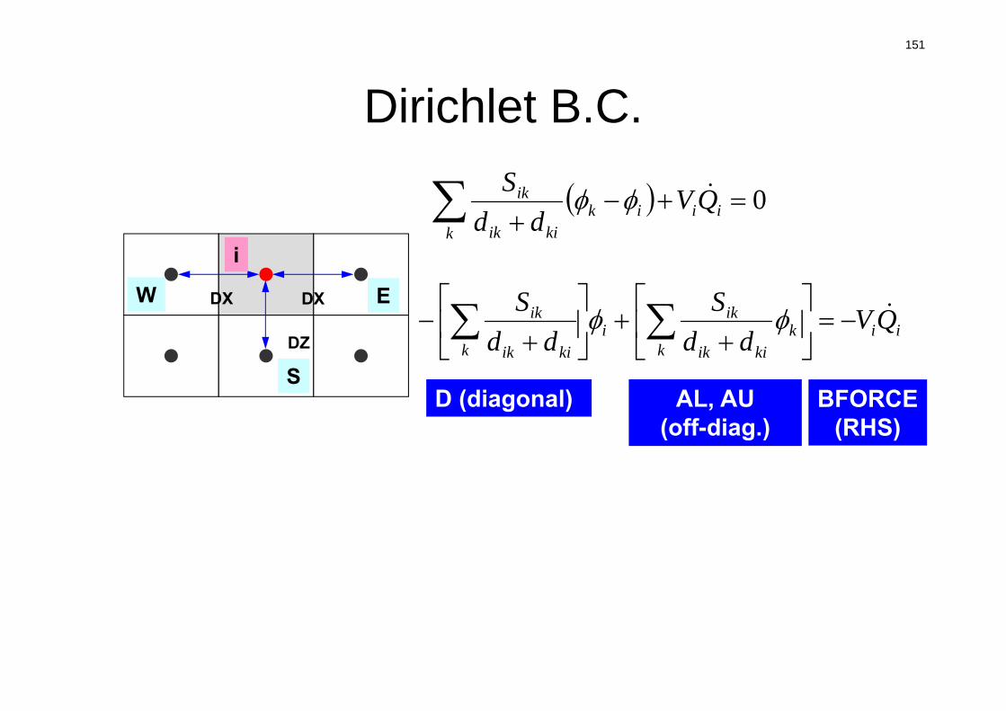
151
Dirichlet B.C.
DX DX
DZ
i
W E
S
0 ii
kik
kiik
ik QVdd
S
iik
kkiik
iki
k kiik
ik QVdd
Sdd
S
D (diagonal) BFORCE(RHS)
AL, AU(off-diag.)
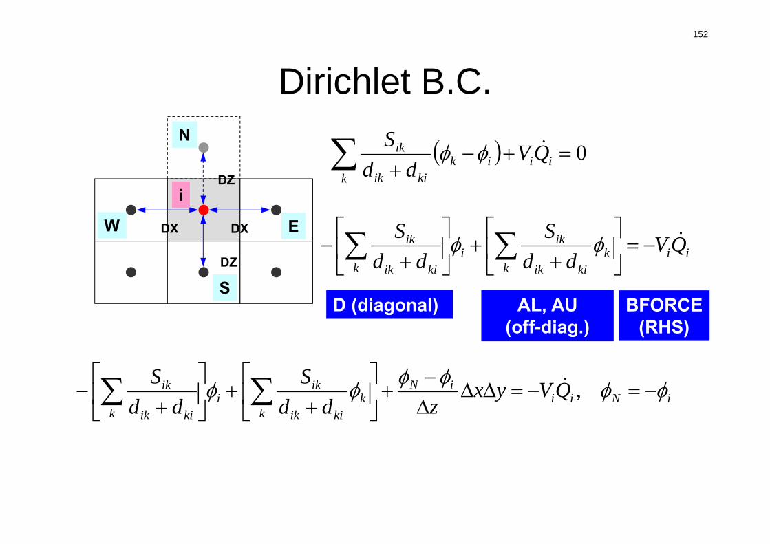
152
Dirichlet B.C.
DX DX
DZ
DZ
i
W E
S
N 0
iik
ikkiik
ik QVdd
S
iNiiiN
kk
kiik
iki
k kiik
ik QVyxzdd
Sdd
S
,
D (diagonal) BFORCE(RHS)
AL, AU(off-diag.)
iik
kkiik
iki
k kiik
ik QVdd
Sdd
S
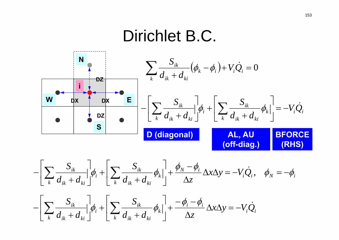
153
Dirichlet B.C.
DX DX
DZ
DZ
i
W E
S
N 0
iik
ikkiik
ik QVdd
S
iiii
kk
kiik
iki
k kiik
ik QVyxzdd
Sdd
S
D (diagonal) BFORCE(RHS)
AL, AU(off-diag.)
iNiiiN
kk
kiik
iki
k kiik
ik QVyxzdd
Sdd
S
,
iik
kkiik
iki
k kiik
ik QVdd
Sdd
S

154
Dirichlet B.C.
DX DX
DZ
DZ
i
W E
S
N 0
iik
ikkiik
ik QVdd
S
iii
kk
kiik
iki
k kiik
ik QVyxzdd
Sdd
S
2
D (diagonal) BFORCE(RHS)
AL, AU(off-diag.)
iik
kkiik
iki
k kiik
ik QVdd
Sdd
S
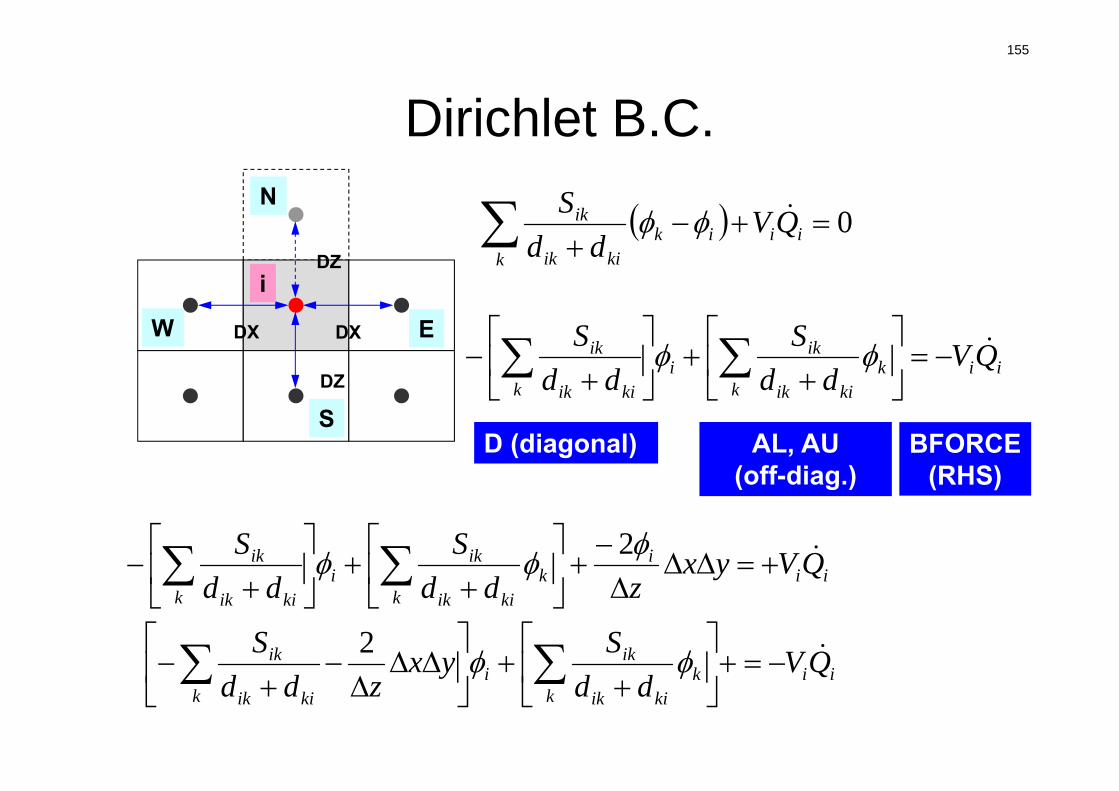
155
Dirichlet B.C.
DX DX
DZ
DZ
i
W E
S
N 0
iik
ikkiik
ik QVdd
S
iik
kkiik
iki
k kiik
ik QVdd
Syxzdd
S
2
D (diagonal) BFORCE(RHS)
AL, AU(off-diag.)
iii
kk
kiik
iki
k kiik
ik QVyxzdd
Sdd
S
2
iik
kkiik
iki
k kiik
ik QVdd
Sdd
S
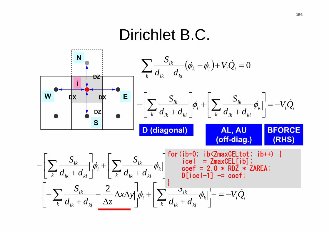
156
Dirichlet B.C.
DX DX
DZ
DZ
i
W E
S
N 0
iik
ikkiik
ik QVdd
S
D (diagonal) BFORCE(RHS)
AL, AU(off-diag.)
iii
kk
kiik
iki
k kiik
ik QVyxzdd
Sdd
S
2
iik
kkiik
iki
k kiik
ik QVdd
Syxzdd
S
2
for(ib=0; ib<ZmaxCELtot; ib++) {icel = ZmaxCEL[ib];coef = 2.0 * RDZ * ZAREA;D[icel-1] -= coef;
}
iik
kkiik
iki
k kiik
ik QVdd
Sdd
S
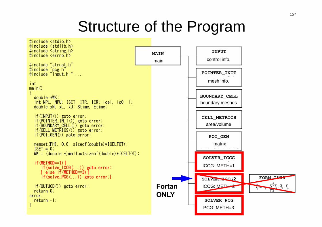
#include <stdio.h>#include <stdlib.h>#include <string.h>#include <errno.h>
#include "struct.h"#include "pcg.h"#include "input.h“ ...
intmain(){double *WK;int NPL, NPU; ISET, ITR, IER; icel, ic0, i;double xN, xL, xU; Stime, Etime;
if(INPUT()) goto error;if(POINTER_INIT()) goto error;if(BOUNDARY_CELL()) goto error;if(CELL_METRICS()) goto error;if(POI_GEN()) goto error;
memset(PHI, 0.0, sizeof(double)*ICELTOT);ISET = 0;WK = (double *)malloc(sizeof(double)*ICELTOT);
if(METHOD==1){if(solve_ICCG(...)) goto error;} else if(METHOD==3){if(solve_PCG(...)) goto error;}
if(OUTUCD()) goto error;return 0;
error:return -1;
}
157
Structure of the ProgramMAIN
メインルーチン
INPUT制御ファイル読込INPUT.DAT
POINTER_INITメッシュファイル読込
mesh.dat
BOUNDARY_CELL=0を設定する要素の探索
CELL_METRICS表面積,体積等の計算
POI_GEN行列コネクティビティ生成,各成分の計算,境界条件
SOLVER_ICCGICCG法ソルバー
METHOD=1
SOLVER_ICCG2ICCG法ソルバー
METHOD=2
SOLVER_PCGICCG法ソルバー
METHOD=3
FORM_ILU0
jkk
j
kikijij ldlal ~~~~ 1
1
main control info.
mesh info.
boundary meshes
area/volume
matrix
ICCG: METH=1
ICCG: METH=2
PCG: METH=3
FortanONLY
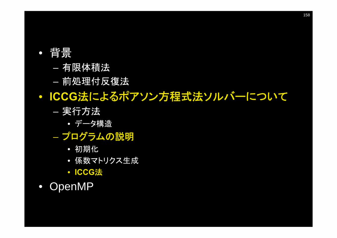
158
• 背景
– 有限体積法
– 前処理付反復法
• ICCG法によるポアソン方程式法ソルバーについて
– 実行方法• データ構造
– プログラムの説明• 初期化
• 係数マトリクス生成
• ICCG法
• OpenMP
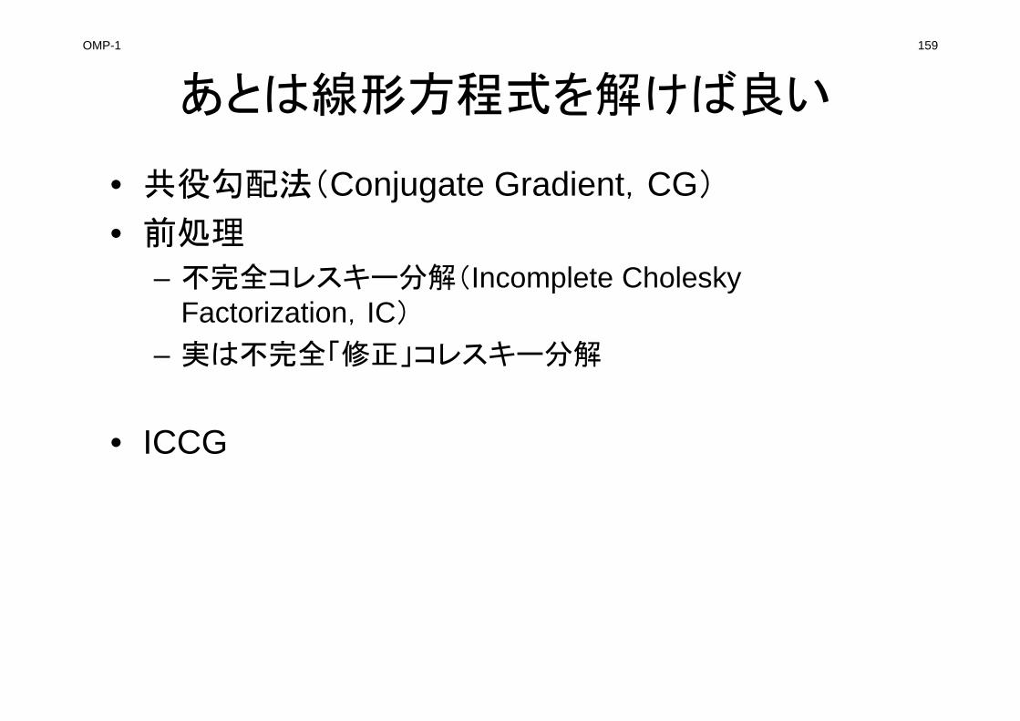
OMP-1 159
あとは線形方程式を解けば良い
• 共役勾配法(Conjugate Gradient,CG)
• 前処理
– 不完全コレスキー分解(Incomplete Cholesky Factorization,IC)
– 実は不完全「修正」コレスキー分解
• ICCG
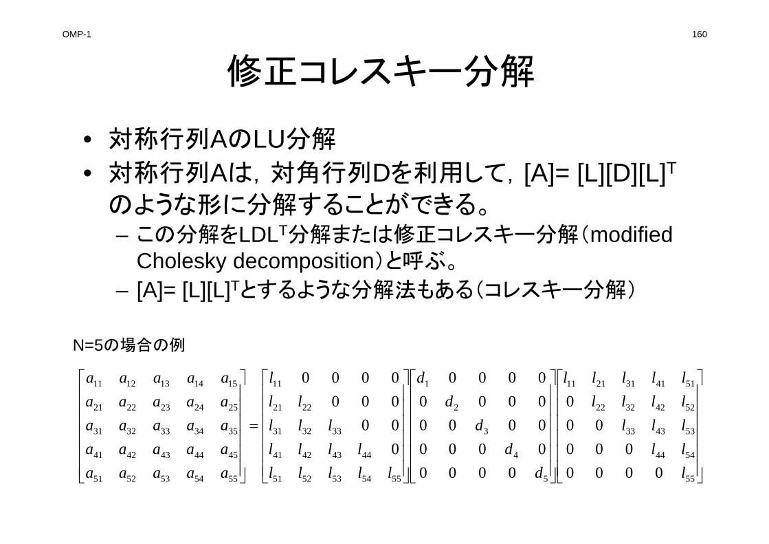
OMP-1 160
修正コレスキー分解
• 対称行列AのLU分解
• 対称行列Aは,対角行列Dを利用して,[A]= [L][D][L]Tのような形に分解することができる。– この分解をLDLT分解または修正コレスキー分解(modified
Cholesky decomposition)と呼ぶ。
– [A]= [L][L]Tとするような分解法もある(コレスキー分解)
55
5444
534333
52423222
5141312111
5
4
3
2
1
5554535251
44434241
333231
2221
11
5554535251
4544434241
3534333231
2524232221
1514131211
0000000
000
00000000000000000000
0000000000
lllllllllllllll
dd
dd
d
lllllllll
lllll
l
aaaaaaaaaaaaaaaaaaaaaaaaa
N=5の場合の例
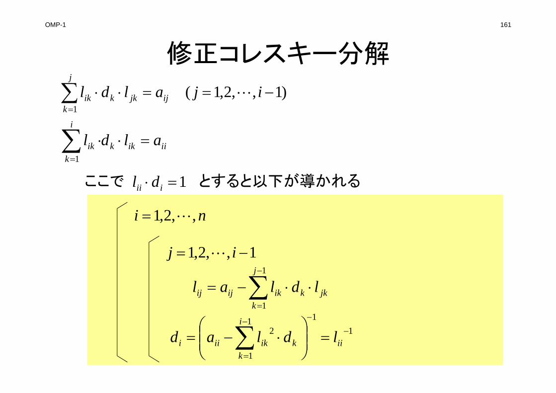
OMP-1 161
修正コレスキー分解
1 iii dlここで とすると以下が導かれる
jkk
j
kikijij ldlal
1
1
ni ,,2,1
1,,2,1 ij
111
1
2
iik
i
kikiii ldlad
)1,,2,1(1
ijaldl ijjkk
j
kik
iiikk
i
kik aldl
1
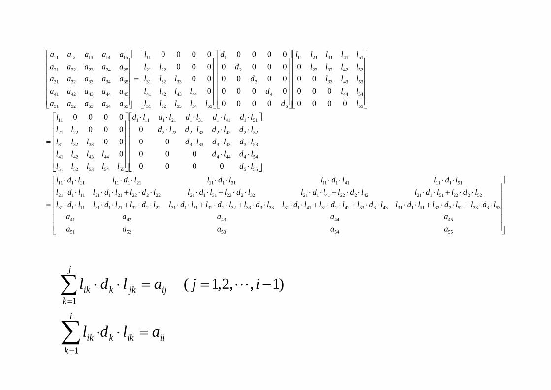
5554535251
4544434241
533335223251131433334223241131333333223231131222322113111131
522225112142222411213222231121222222112111121
5111141111311112111111111
555
544444
533433333
522422322222
511411311211111
5554535251
44434241
333231
2221
11
55
5444
534333
52423222
5141312111
5
4
3
2
1
5554535251
44434241
333231
2221
11
5554535251
4544434241
3534333231
2524232221
1514131211
0000000
000
0000000000
0000000
000
00000000000000000000
0000000000
aaaaaaaaaa
ldlldlldlldlldlldlldlldlldlldlldlldlldlldlldlldlldlldlldlldlldl
ldlldlldlldlldl
ldldldldldldldldldldldldldldld
lllllllll
lllll
l
lllllllllllllll
dd
dd
d
lllllllll
lllll
l
aaaaaaaaaaaaaaaaaaaaaaaaa
)1,,2,1(1
ijaldl ijjkk
j
kik
iiikk
i
kik aldl
1
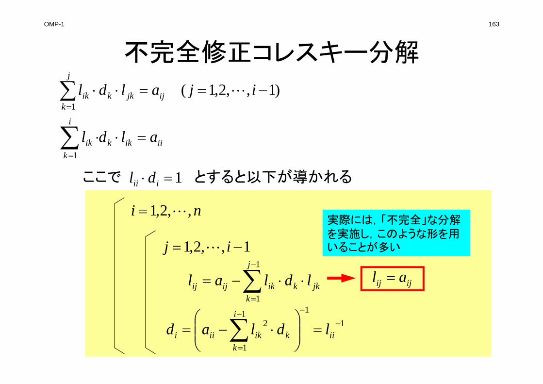
OMP-1 163
不完全修正コレスキー分解
)1,,2,1(1
ijaldl ijjkk
j
kik
iiikk
i
kik aldl
1
1 iii dlここで とすると以下が導かれる
実際には,「不完全」な分解を実施し,このような形を用いることが多い
jkk
j
kikijij ldlal
1
1
ni ,,2,1
1,,2,1 ij
111
1
2
iik
i
kikiii ldlad
ijij al
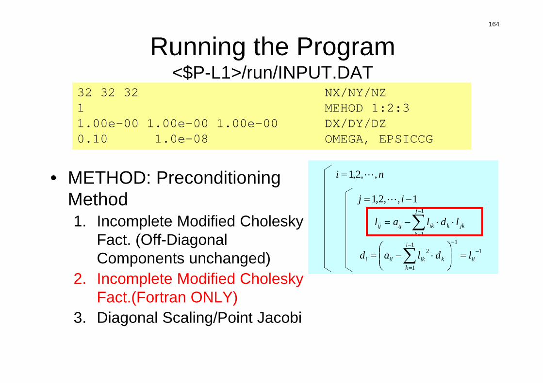
164
Running the Program<$P-L1>/run/INPUT.DAT
32 32 32 NX/NY/NZ1 MEHOD 1:2:31.00e-00 1.00e-00 1.00e-00 DX/DY/DZ0.10 1.0e-08 OMEGA, EPSICCG
• METHOD: Preconditioning Method1. Incomplete Modified Cholesky
Fact. (Off-Diagonal Components unchanged)
2. Incomplete Modified Cholesky Fact.(Fortran ONLY)
3. Diagonal Scaling/Point Jacobi
jkk
j
kikijij ldlal
1
1
ni ,,2,1
1,,2,1 ij
111
1
2
iik
i
kikiii ldlad
jkk
j
kikijij ldlal
1
1
ni ,,2,1
1,,2,1 ij
111
1
2
iik
i
kikiii ldlad
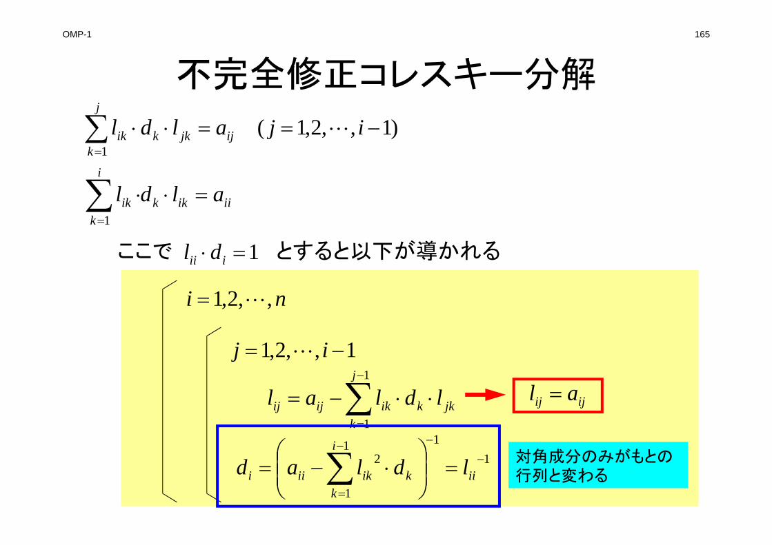
OMP-1 165
不完全修正コレスキー分解
1 iii dlここで とすると以下が導かれる
jkk
j
kikijij ldlal
1
1
ni ,,2,1
1,,2,1 ij
111
1
2
iik
i
kikiii ldlad
ijij al
対角成分のみがもとの行列と変わる
iiikk
i
kik aldl
1
)1,,2,1(1
ijaldl ijjkk
j
kik
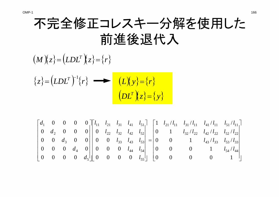
OMP-1 166
不完全修正コレスキー分解を使用した前進後退代入
rLDLz T 1
rzLDLzM T
ryL
yzDLT
10000/1000//100///10////1
0000000
000
00000000000000000000
4454
33533343
225222422232
1151114111311121
55
5444
534333
52423222
5141312111
5
4
3
2
1
llllllllllllllllllll
lllllllllllllll
dd
dd
d
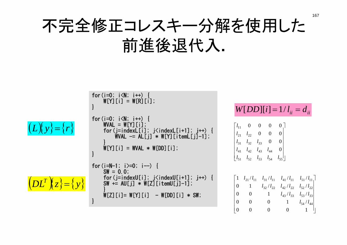
167
不完全修正コレスキー分解を使用した前進後退代入.
5554535251
44434241
333231
2221
11
0000000000
lllllllll
lllll
l
10000/1000//100///10////1
4454
33533343
225222422232
1151114111311121
llllllllllllllllllll
for(i=0; i<N; i++) {W[Y][i] = W[R][i];
}
for(i=0; i<N; i++) {WVAL = W[Y][i];for(j=indexL[i]; j<indexL[i+1]; j++) {
WVAL -= AL[j] * W[Y][itemL[j]-1];}W[Y][i] = WVAL * W[DD][i];
}
for(i=N-1; i>=0; i--) {SW = 0.0;for(j=indexU[i]; j<indexU[i+1]; j++) {SW += AU[j] * W[Z][itemU[j]-1];}W[Z][i]= W[Y][i] - W[DD][i] * SW;
}
iiii dliDDW /1]][[
ryL
yzDLT
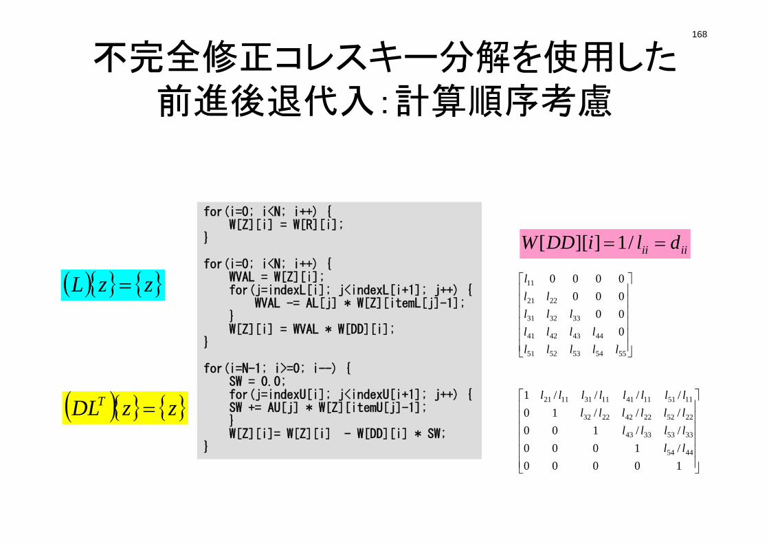
168
不完全修正コレスキー分解を使用した前進後退代入:計算順序考慮
5554535251
44434241
333231
2221
11
0000000000
lllllllll
lllll
l
10000/1000//100///10////1
4454
33533343
225222422232
1151114111311121
llllllllllllllllllll
iiii dliDDW /1]][[
for(i=0; i<N; i++) {W[Z][i] = W[R][i];
}
for(i=0; i<N; i++) {WVAL = W[Z][i];for(j=indexL[i]; j<indexL[i+1]; j++) {
WVAL -= AL[j] * W[Z][itemL[j]-1];}W[Z][i] = WVAL * W[DD][i];
}
for(i=N-1; i>=0; i--) {SW = 0.0;for(j=indexU[i]; j<indexU[i+1]; j++) {SW += AU[j] * W[Z][itemU[j]-1];}W[Z][i]= W[Z][i] - W[DD][i] * SW;
}
zzL
zzDLT
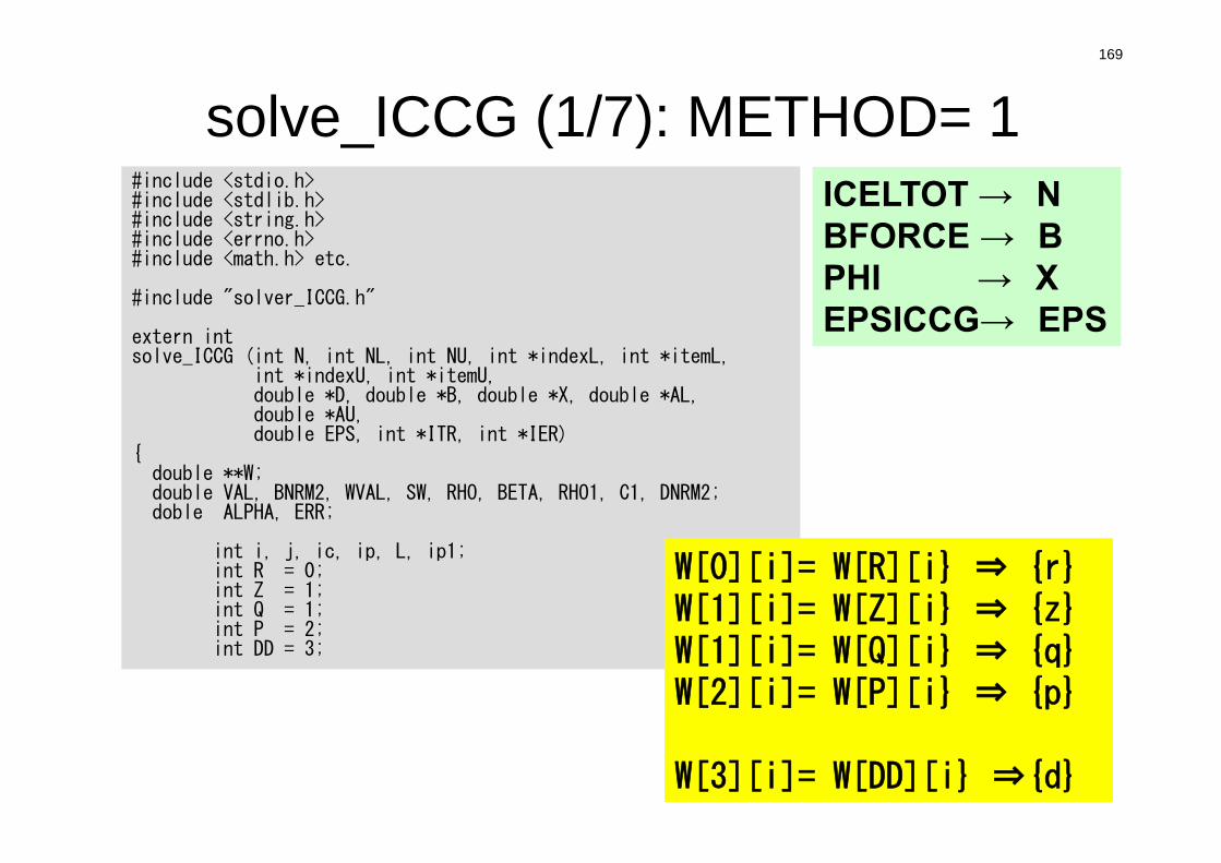
169
solve_ICCG (1/7): METHOD= 1#include <stdio.h>#include <stdlib.h>#include <string.h>#include <errno.h>#include <math.h> etc.
#include "solver_ICCG.h"
extern intsolve_ICCG (int N, int NL, int NU, int *indexL, int *itemL,
int *indexU, int *itemU,double *D, double *B, double *X, double *AL, double *AU,double EPS, int *ITR, int *IER)
{double **W;double VAL, BNRM2, WVAL, SW, RHO, BETA, RHO1, C1, DNRM2;doble ALPHA, ERR;
int i, j, ic, ip, L, ip1;int R = 0;int Z = 1;int Q = 1;int P = 2;int DD = 3;
W[0][i]= W[R][i} ⇒ {r}W[1][i]= W[Z][i} ⇒ {z}W[1][i]= W[Q][i} ⇒ {q}W[2][i]= W[P][i} ⇒ {p}
W[3][i]= W[DD][i} ⇒{d}
ICELTOT → NBFORCE → BPHI → XEPSICCG→ EPS
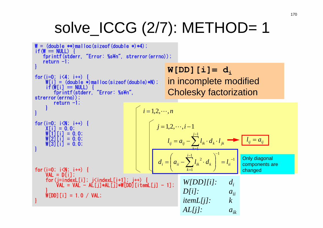
170
solve_ICCG (2/7): METHOD= 1W = (double **)malloc(sizeof(double *)*4);if(W == NULL) {
fprintf(stderr, "Error: %s¥n", strerror(errno));return -1;
}
for(i=0; i<4; i++) {W[i] = (double *)malloc(sizeof(double)*N);if(W[i] == NULL) {
fprintf(stderr, "Error: %s¥n", strerror(errno));
return -1;}
}
for(i=0; i<N; i++) {X[i] = 0.0;W[1][i] = 0.0;W[2][i] = 0.0;W[3][i] = 0.0;
}
for(i=0; i<N; i++) {VAL = D[i];for(j=indexL[i]; j<indexL[i+1]; j++) {
VAL = VAL - AL[j]*AL[j]*W[DD][itemL[j] - 1];}W[DD][i] = 1.0 / VAL;
}
W[DD][i]= diin incomplete modified Cholesky factorization
jkk
j
kikijij ldlal
1
1
ni ,,2,1
1,,2,1 ij
111
1
2
iik
i
kikiii ldlad
ijij al
Only diagonal components are changed
W[DD][i]: diD[i]: aiiitemL[j]: kAL[j]: aik
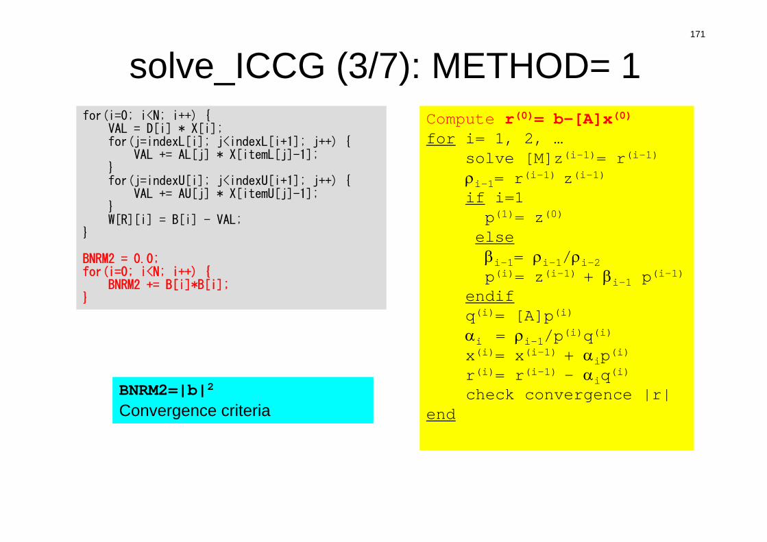
171
solve_ICCG (3/7): METHOD= 1for(i=0; i<N; i++) {
VAL = D[i] * X[i];for(j=indexL[i]; j<indexL[i+1]; j++) {
VAL += AL[j] * X[itemL[j]-1];}for(j=indexU[i]; j<indexU[i+1]; j++) {
VAL += AU[j] * X[itemU[j]-1];}W[R][i] = B[i] - VAL;
}
BNRM2 = 0.0;for(i=0; i<N; i++) {
BNRM2 += B[i]*B[i];}
Compute r(0)= b-[A]x(0)
for i= 1, 2, …solve [M]z(i-1)= r(i-1)
i-1= r(i-1) z(i-1)if i=1p(1)= z(0)
elsei-1= i-1/i-2p(i)= z(i-1) + i-1 p(i-1)
endifq(i)= [A]p(i)
i = i-1/p(i)q(i)x(i)= x(i-1) + ip(i)r(i)= r(i-1) - iq(i)check convergence |r|
end
BNRM2=|b|2
Convergence criteria
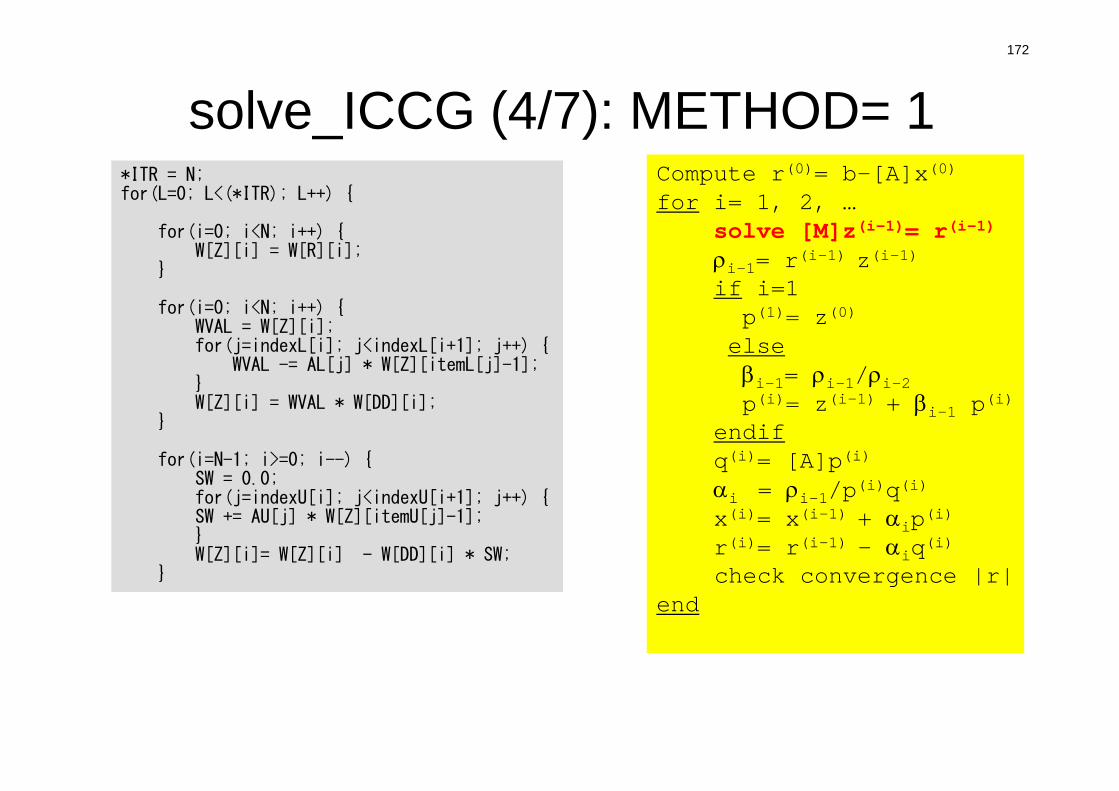
172
solve_ICCG (4/7): METHOD= 1*ITR = N;for(L=0; L<(*ITR); L++) {
for(i=0; i<N; i++) {W[Z][i] = W[R][i];
}
for(i=0; i<N; i++) {WVAL = W[Z][i];for(j=indexL[i]; j<indexL[i+1]; j++) {
WVAL -= AL[j] * W[Z][itemL[j]-1];}W[Z][i] = WVAL * W[DD][i];
}
for(i=N-1; i>=0; i--) {SW = 0.0;for(j=indexU[i]; j<indexU[i+1]; j++) {SW += AU[j] * W[Z][itemU[j]-1];}W[Z][i]= W[Z][i] - W[DD][i] * SW;
}
Compute r(0)= b-[A]x(0)
for i= 1, 2, …solve [M]z(i-1)= r(i-1)
i-1= r(i-1) z(i-1)if i=1p(1)= z(0)
elsei-1= i-1/i-2p(i)= z(i-1) + i-1 p(i)
endifq(i)= [A]p(i)
i = i-1/p(i)q(i)x(i)= x(i-1) + ip(i)r(i)= r(i-1) - iq(i)check convergence |r|
end
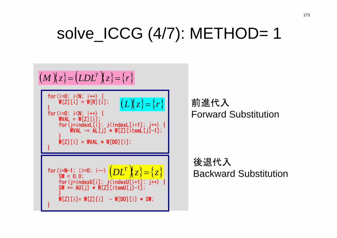
for(i=0; i<N; i++) {W[Z][i] = W[R][i];
}for(i=0; i<N; i++) {
WVAL = W[Z][i];for(j=indexL[i]; j<indexL[i+1]; j++) {
WVAL -= AL[j] * W[Z][itemL[j]-1];}W[Z][i] = WVAL * W[DD][i];
}
for(i=N-1; i>=0; i--) {SW = 0.0;for(j=indexU[i]; j<indexU[i+1]; j++) {SW += AU[j] * W[Z][itemU[j]-1];}W[Z][i]= W[Z][i] - W[DD][i] * SW;
}
173
solve_ICCG (4/7): METHOD= 1
rzL
zzDLT
rzLDLzM T
前進代入Forward Substitution
後退代入Backward Substitution
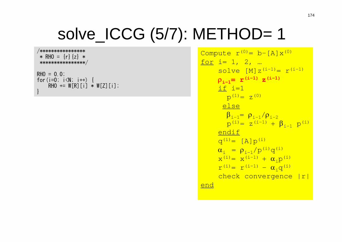
174
solve_ICCG (5/7): METHOD= 1/***************** RHO = {r}{z} *****************/
RHO = 0.0;for(i=0; i<N; i++) {
RHO += W[R][i] * W[Z][i];}
Compute r(0)= b-[A]x(0)
for i= 1, 2, …solve [M]z(i-1)= r(i-1)
i-1= r(i-1) z(i-1)if i=1p(1)= z(0)
elsei-1= i-1/i-2p(i)= z(i-1) + i-1 p(i)
endifq(i)= [A]p(i)
i = i-1/p(i)q(i)x(i)= x(i-1) + ip(i)r(i)= r(i-1) - iq(i)check convergence |r|
end
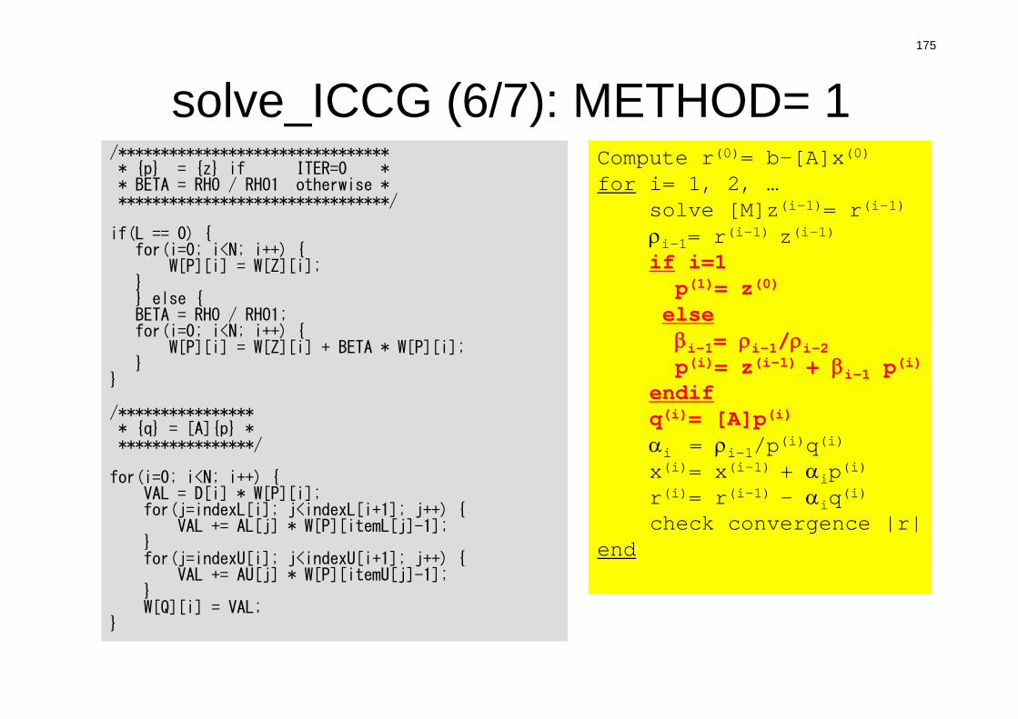
175
solve_ICCG (6/7): METHOD= 1/********************************* {p} = {z} if ITER=0 ** BETA = RHO / RHO1 otherwise *********************************/
if(L == 0) {for(i=0; i<N; i++) {
W[P][i] = W[Z][i];}} else {BETA = RHO / RHO1;for(i=0; i<N; i++) {
W[P][i] = W[Z][i] + BETA * W[P][i];}
}
/***************** {q} = [A]{p} *****************/
for(i=0; i<N; i++) {VAL = D[i] * W[P][i];for(j=indexL[i]; j<indexL[i+1]; j++) {
VAL += AL[j] * W[P][itemL[j]-1];}for(j=indexU[i]; j<indexU[i+1]; j++) {
VAL += AU[j] * W[P][itemU[j]-1];}W[Q][i] = VAL;
}
Compute r(0)= b-[A]x(0)
for i= 1, 2, …solve [M]z(i-1)= r(i-1)
i-1= r(i-1) z(i-1)if i=1p(1)= z(0)
elsei-1= i-1/i-2p(i)= z(i-1) + i-1 p(i)
endifq(i)= [A]p(i)
i = i-1/p(i)q(i)x(i)= x(i-1) + ip(i)r(i)= r(i-1) - iq(i)check convergence |r|
end
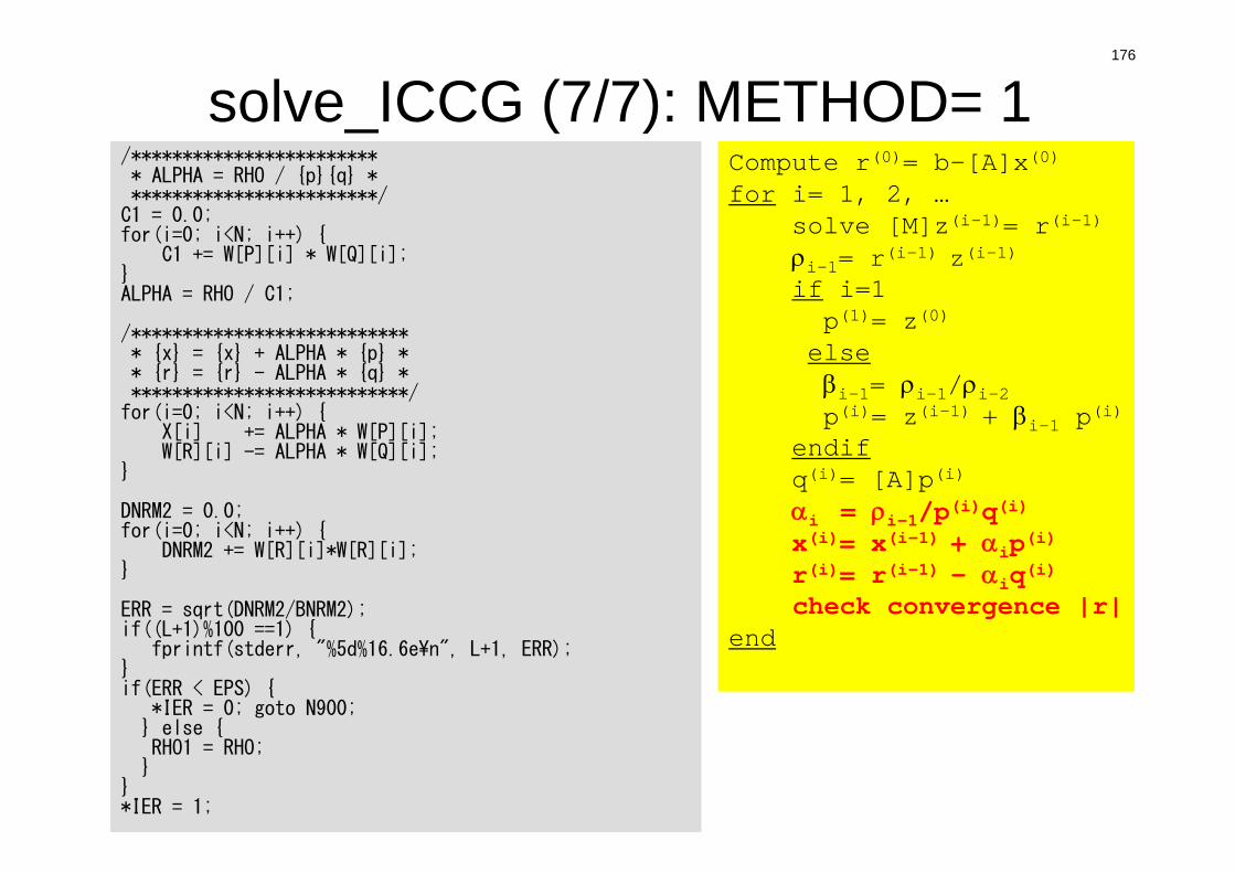
176
solve_ICCG (7/7): METHOD= 1/************************* ALPHA = RHO / {p}{q} *************************/
C1 = 0.0;for(i=0; i<N; i++) {
C1 += W[P][i] * W[Q][i];}ALPHA = RHO / C1;
/**************************** {x} = {x} + ALPHA * {p} ** {r} = {r} - ALPHA * {q} ****************************/
for(i=0; i<N; i++) {X[i] += ALPHA * W[P][i];W[R][i] -= ALPHA * W[Q][i];
}
DNRM2 = 0.0;for(i=0; i<N; i++) {
DNRM2 += W[R][i]*W[R][i];}
ERR = sqrt(DNRM2/BNRM2);if((L+1)%100 ==1) {
fprintf(stderr, "%5d%16.6e¥n", L+1, ERR);}if(ERR < EPS) {
*IER = 0; goto N900;} else {RHO1 = RHO;
}}*IER = 1;
Compute r(0)= b-[A]x(0)
for i= 1, 2, …solve [M]z(i-1)= r(i-1)
i-1= r(i-1) z(i-1)if i=1p(1)= z(0)
elsei-1= i-1/i-2p(i)= z(i-1) + i-1 p(i)
endifq(i)= [A]p(i)
i = i-1/p(i)q(i)x(i)= x(i-1) + ip(i)r(i)= r(i-1) - iq(i)check convergence |r|
end
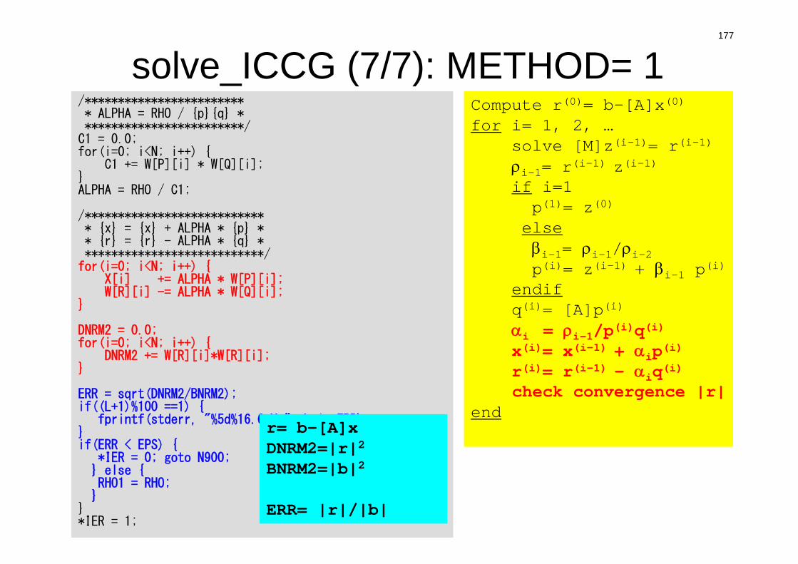
/************************* ALPHA = RHO / {p}{q} *************************/
C1 = 0.0;for(i=0; i<N; i++) {
C1 += W[P][i] * W[Q][i];}ALPHA = RHO / C1;
/**************************** {x} = {x} + ALPHA * {p} ** {r} = {r} - ALPHA * {q} ****************************/
for(i=0; i<N; i++) {X[i] += ALPHA * W[P][i];W[R][i] -= ALPHA * W[Q][i];
}
DNRM2 = 0.0;for(i=0; i<N; i++) {
DNRM2 += W[R][i]*W[R][i];}
ERR = sqrt(DNRM2/BNRM2);if((L+1)%100 ==1) {
fprintf(stderr, "%5d%16.6e¥n", L+1, ERR);}if(ERR < EPS) {
*IER = 0; goto N900;} else {RHO1 = RHO;
}}*IER = 1;
Compute r(0)= b-[A]x(0)
for i= 1, 2, …solve [M]z(i-1)= r(i-1)
i-1= r(i-1) z(i-1)if i=1p(1)= z(0)
elsei-1= i-1/i-2p(i)= z(i-1) + i-1 p(i)
endifq(i)= [A]p(i)
i = i-1/p(i)q(i)x(i)= x(i-1) + ip(i)r(i)= r(i-1) - iq(i)check convergence |r|
end
177
solve_ICCG (7/7): METHOD= 1
r= b-[A]xDNRM2=|r|2
BNRM2=|b|2
ERR= |r|/|b|
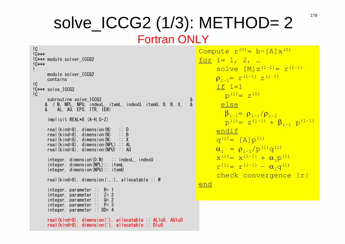
178
solve_ICCG2 (1/3): METHOD= 2Fortran ONLY
!C!C***!C*** module solver_ICCG2!C***!
module solver_ICCG2contains
!C!C*** solve_ICCG2!C
subroutine solve_ICCG2 & & ( N, NPL, NPU, indexL, itemL, indexU, itemU, D, B, X, && AL, AU, EPS, ITR, IER)
implicit REAL*8 (A-H,O-Z)
real(kind=8), dimension(N) :: Dreal(kind=8), dimension(N) :: Breal(kind=8), dimension(N) :: Xreal(kind=8), dimension(NPL) :: ALreal(kind=8), dimension(NPU) :: AU
integer, dimension(0:N) :: indexL, indexUinteger, dimension(NPL):: itemLinteger, dimension(NPU):: itemU
real(kind=8), dimension(:,:), allocatable :: W
integer, parameter :: R= 1integer, parameter :: Z= 2integer, parameter :: Q= 2integer, parameter :: P= 3integer, parameter :: DD= 4
real(kind=8), dimension(:), allocatable :: ALlu0, AUlu0real(kind=8), dimension(:), allocatable :: Dlu0
Compute r(0)= b-[A]x(0)
for i= 1, 2, …solve [M]z(i-1)= r(i-1)
i-1= r(i-1) z(i-1)if i=1p(1)= z(0)
elsei-1= i-1/i-2p(i)= z(i-1) + i-1 p(i-1)
endifq(i)= [A]p(i)
i = i-1/p(i)q(i)x(i)= x(i-1) + ip(i)r(i)= r(i-1) - iq(i)check convergence |r|
end
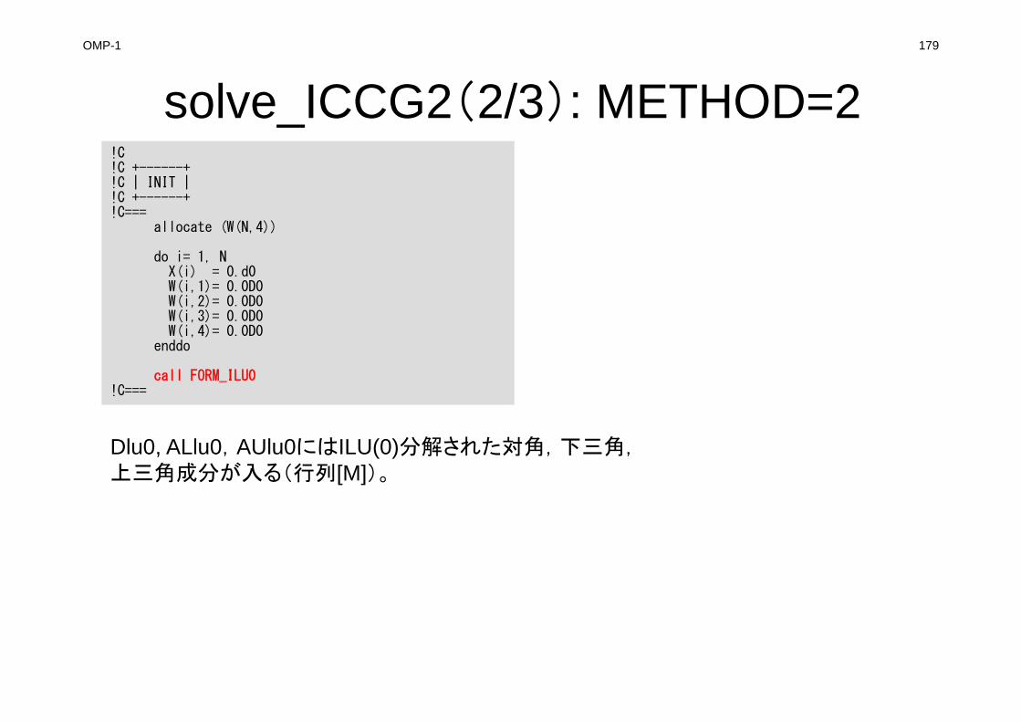
OMP-1 179
solve_ICCG2(2/3): METHOD=2!C!C +------+!C | INIT |!C +------+!C===
allocate (W(N,4))
do i= 1, NX(i) = 0.d0W(i,1)= 0.0D0W(i,2)= 0.0D0W(i,3)= 0.0D0W(i,4)= 0.0D0
enddo
call FORM_ILU0!C===
Dlu0, ALlu0,AUlu0にはILU(0)分解された対角,下三角,上三角成分が入る(行列[M])。
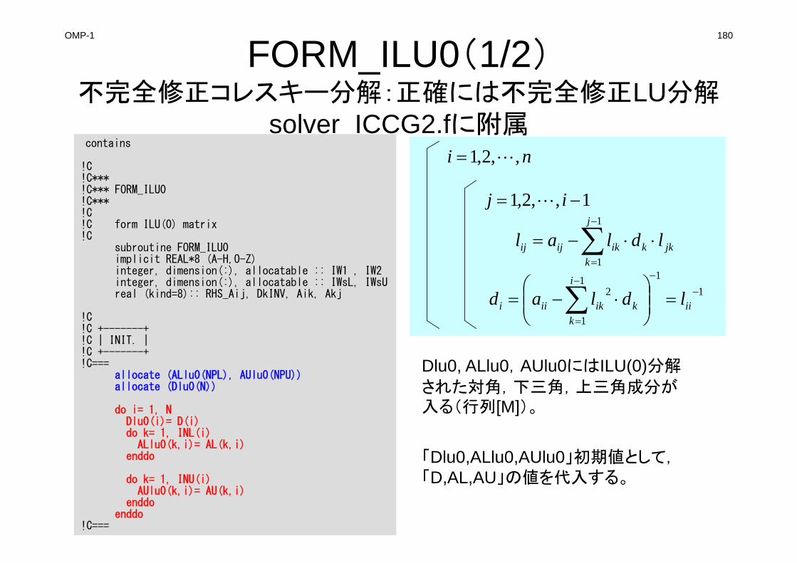
OMP-1 180
FORM_ILU0(1/2)不完全修正コレスキー分解:正確には不完全修正LU分解
solver_ICCG2.fに附属contains
!C!C***!C*** FORM_ILU0!C***!C!C form ILU(0) matrix!C
subroutine FORM_ILU0implicit REAL*8 (A-H,O-Z)integer, dimension(:), allocatable :: IW1 , IW2integer, dimension(:), allocatable :: IWsL, IWsUreal (kind=8):: RHS_Aij, DkINV, Aik, Akj
!C!C +-------+!C | INIT. |!C +-------+!C===
allocate (ALlu0(NPL), AUlu0(NPU))allocate (Dlu0(N))
do i= 1, NDlu0(i)= D(i)do k= 1, INL(i)ALlu0(k,i)= AL(k,i)
enddo
do k= 1, INU(i)AUlu0(k,i)= AU(k,i)
enddoenddo
!C===
「Dlu0,ALlu0,AUlu0」初期値として,「D,AL,AU」の値を代入する。
jkk
j
kikijij ldlal
1
1
ni ,,2,1
1,,2,1 ij
111
1
2
iik
i
kikiii ldlad
Dlu0, ALlu0,AUlu0にはILU(0)分解
された対角,下三角,上三角成分が入る(行列[M])。
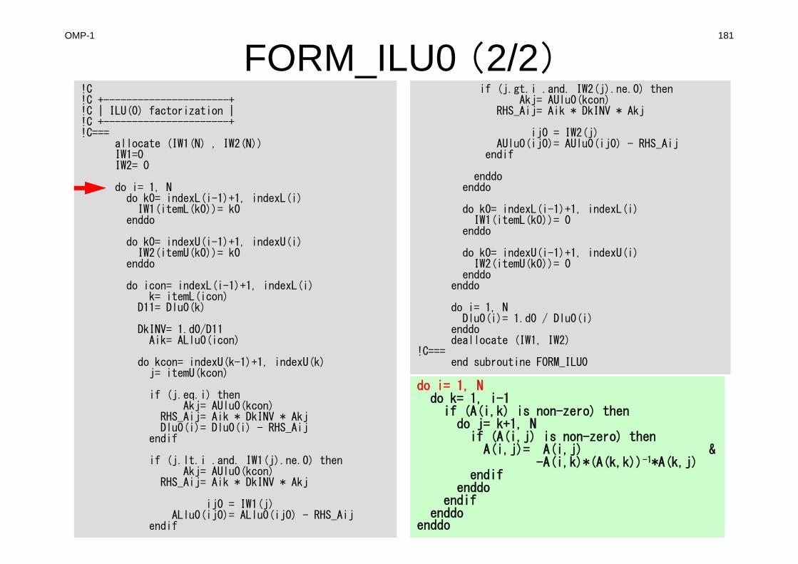
OMP-1 181
FORM_ILU0 (2/2)!C!C +----------------------+!C | ILU(0) factorization |!C +----------------------+!C===
allocate (IW1(N) , IW2(N))IW1=0IW2= 0
do i= 1, Ndo k0= indexL(i-1)+1, indexL(i)IW1(itemL(k0))= k0
enddo
do k0= indexU(i-1)+1, indexU(i)IW2(itemU(k0))= k0
enddo
do icon= indexL(i-1)+1, indexL(i)k= itemL(icon)
D11= Dlu0(k)
DkINV= 1.d0/D11Aik= ALlu0(icon)
do kcon= indexU(k-1)+1, indexU(k)j= itemU(kcon)
if (j.eq.i) thenAkj= AUlu0(kcon)
RHS_Aij= Aik * DkINV * AkjDlu0(i)= Dlu0(i) - RHS_Aij
endif
if (j.lt.i .and. IW1(j).ne.0) thenAkj= AUlu0(kcon)
RHS_Aij= Aik * DkINV * Akj
ij0 = IW1(j)ALlu0(ij0)= ALlu0(ij0) - RHS_Aij
endif
do i= 1, Ndo k= 1, i-1
if (A(i,k) is non-zero) thendo j= k+1, Nif (A(i,j) is non-zero) then
A(i,j)= A(i,j) &-A(i,k)*(A(k,k))-1*A(k,j)
endifenddo
endifenddo
enddo
if (j.gt.i .and. IW2(j).ne.0) thenAkj= AUlu0(kcon)
RHS_Aij= Aik * DkINV * Akj
ij0 = IW2(j)AUlu0(ij0)= AUlu0(ij0) - RHS_Aij
endif
enddoenddo
do k0= indexL(i-1)+1, indexL(i)IW1(itemL(k0))= 0
enddo
do k0= indexU(i-1)+1, indexU(i)IW2(itemU(k0))= 0
enddoenddo
do i= 1, NDlu0(i)= 1.d0 / Dlu0(i)
enddodeallocate (IW1, IW2)
!C===end subroutine FORM_ILU0
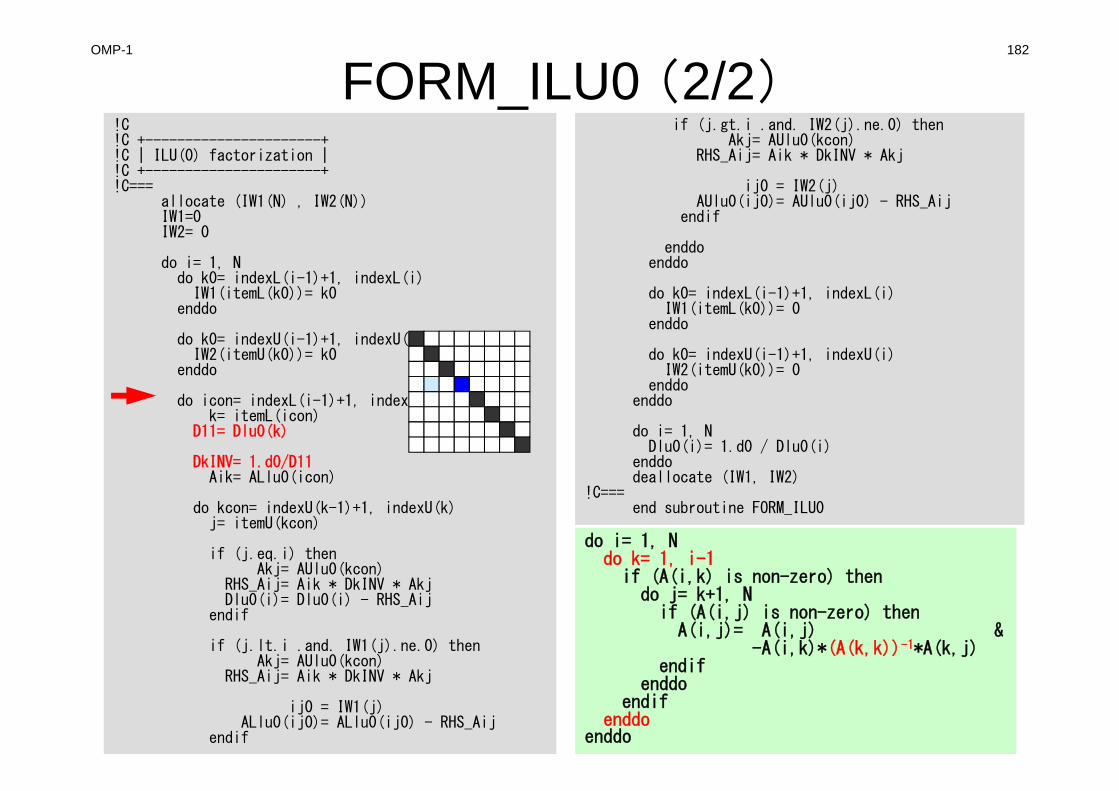
OMP-1 182
FORM_ILU0 (2/2)!C!C +----------------------+!C | ILU(0) factorization |!C +----------------------+!C===
allocate (IW1(N) , IW2(N))IW1=0IW2= 0
do i= 1, Ndo k0= indexL(i-1)+1, indexL(i)IW1(itemL(k0))= k0
enddo
do k0= indexU(i-1)+1, indexU(i)IW2(itemU(k0))= k0
enddo
do icon= indexL(i-1)+1, indexL(i)k= itemL(icon)
D11= Dlu0(k)
DkINV= 1.d0/D11Aik= ALlu0(icon)
do kcon= indexU(k-1)+1, indexU(k)j= itemU(kcon)
if (j.eq.i) thenAkj= AUlu0(kcon)
RHS_Aij= Aik * DkINV * AkjDlu0(i)= Dlu0(i) - RHS_Aij
endif
if (j.lt.i .and. IW1(j).ne.0) thenAkj= AUlu0(kcon)
RHS_Aij= Aik * DkINV * Akj
ij0 = IW1(j)ALlu0(ij0)= ALlu0(ij0) - RHS_Aij
endif
if (j.gt.i .and. IW2(j).ne.0) thenAkj= AUlu0(kcon)
RHS_Aij= Aik * DkINV * Akj
ij0 = IW2(j)AUlu0(ij0)= AUlu0(ij0) - RHS_Aij
endif
enddoenddo
do k0= indexL(i-1)+1, indexL(i)IW1(itemL(k0))= 0
enddo
do k0= indexU(i-1)+1, indexU(i)IW2(itemU(k0))= 0
enddoenddo
do i= 1, NDlu0(i)= 1.d0 / Dlu0(i)
enddodeallocate (IW1, IW2)
!C===end subroutine FORM_ILU0
do i= 1, Ndo k= 1, i-1
if (A(i,k) is non-zero) thendo j= k+1, Nif (A(i,j) is non-zero) then
A(i,j)= A(i,j) &-A(i,k)*(A(k,k))-1*A(k,j)
endifenddo
endifenddo
enddo
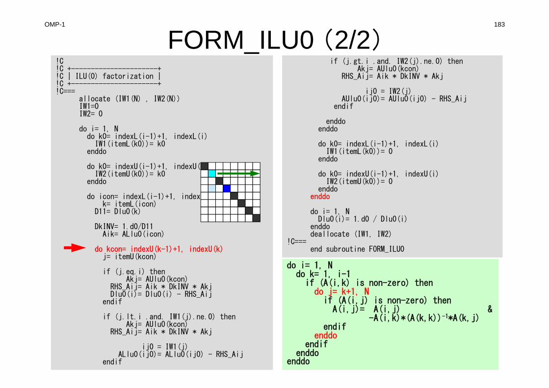
OMP-1 183
FORM_ILU0 (2/2)!C!C +----------------------+!C | ILU(0) factorization |!C +----------------------+!C===
allocate (IW1(N) , IW2(N))IW1=0IW2= 0
do i= 1, Ndo k0= indexL(i-1)+1, indexL(i)IW1(itemL(k0))= k0
enddo
do k0= indexU(i-1)+1, indexU(i)IW2(itemU(k0))= k0
enddo
do icon= indexL(i-1)+1, indexL(i)k= itemL(icon)
D11= Dlu0(k)
DkINV= 1.d0/D11Aik= ALlu0(icon)
do kcon= indexU(k-1)+1, indexU(k)j= itemU(kcon)
if (j.eq.i) thenAkj= AUlu0(kcon)
RHS_Aij= Aik * DkINV * AkjDlu0(i)= Dlu0(i) - RHS_Aij
endif
if (j.lt.i .and. IW1(j).ne.0) thenAkj= AUlu0(kcon)
RHS_Aij= Aik * DkINV * Akj
ij0 = IW1(j)ALlu0(ij0)= ALlu0(ij0) - RHS_Aij
endif
if (j.gt.i .and. IW2(j).ne.0) thenAkj= AUlu0(kcon)
RHS_Aij= Aik * DkINV * Akj
ij0 = IW2(j)AUlu0(ij0)= AUlu0(ij0) - RHS_Aij
endif
enddoenddo
do k0= indexL(i-1)+1, indexL(i)IW1(itemL(k0))= 0
enddo
do k0= indexU(i-1)+1, indexU(i)IW2(itemU(k0))= 0
enddoenddo
do i= 1, NDlu0(i)= 1.d0 / Dlu0(i)
enddodeallocate (IW1, IW2)
!C===end subroutine FORM_ILU0
do i= 1, Ndo k= 1, i-1
if (A(i,k) is non-zero) thendo j= k+1, Nif (A(i,j) is non-zero) then
A(i,j)= A(i,j) &-A(i,k)*(A(k,k))-1*A(k,j)
endifenddo
endifenddo
enddo
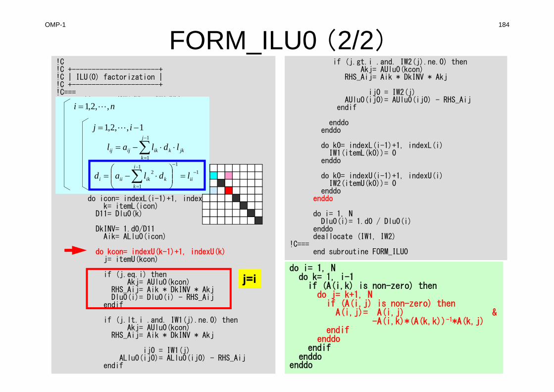
OMP-1 184
FORM_ILU0 (2/2)!C!C +----------------------+!C | ILU(0) factorization |!C +----------------------+!C===
allocate (IW1(N) , IW2(N))IW1=0IW2= 0
do i= 1, Ndo k0= indexL(i-1)+1, indexL(i)IW1(itemL(k0))= k0
enddo
do k0= indexU(i-1)+1, indexU(i)IW2(itemU(k0))= k0
enddo
do icon= indexL(i-1)+1, indexL(i)k= itemL(icon)
D11= Dlu0(k)
DkINV= 1.d0/D11Aik= ALlu0(icon)
do kcon= indexU(k-1)+1, indexU(k)j= itemU(kcon)
if (j.eq.i) thenAkj= AUlu0(kcon)
RHS_Aij= Aik * DkINV * AkjDlu0(i)= Dlu0(i) - RHS_Aij
endif
if (j.lt.i .and. IW1(j).ne.0) thenAkj= AUlu0(kcon)
RHS_Aij= Aik * DkINV * Akj
ij0 = IW1(j)ALlu0(ij0)= ALlu0(ij0) - RHS_Aij
endif
if (j.gt.i .and. IW2(j).ne.0) thenAkj= AUlu0(kcon)
RHS_Aij= Aik * DkINV * Akj
ij0 = IW2(j)AUlu0(ij0)= AUlu0(ij0) - RHS_Aij
endif
enddoenddo
do k0= indexL(i-1)+1, indexL(i)IW1(itemL(k0))= 0
enddo
do k0= indexU(i-1)+1, indexU(i)IW2(itemU(k0))= 0
enddoenddo
do i= 1, NDlu0(i)= 1.d0 / Dlu0(i)
enddodeallocate (IW1, IW2)
!C===end subroutine FORM_ILU0
do i= 1, Ndo k= 1, i-1
if (A(i,k) is non-zero) thendo j= k+1, Nif (A(i,j) is non-zero) then
A(i,j)= A(i,j) &-A(i,k)*(A(k,k))-1*A(k,j)
endifenddo
endifenddo
enddo
j=i
jkk
j
kikijij ldlal
1
1
ni ,,2,1
1,,2,1 ij
111
1
2
iik
i
kikiii ldlad
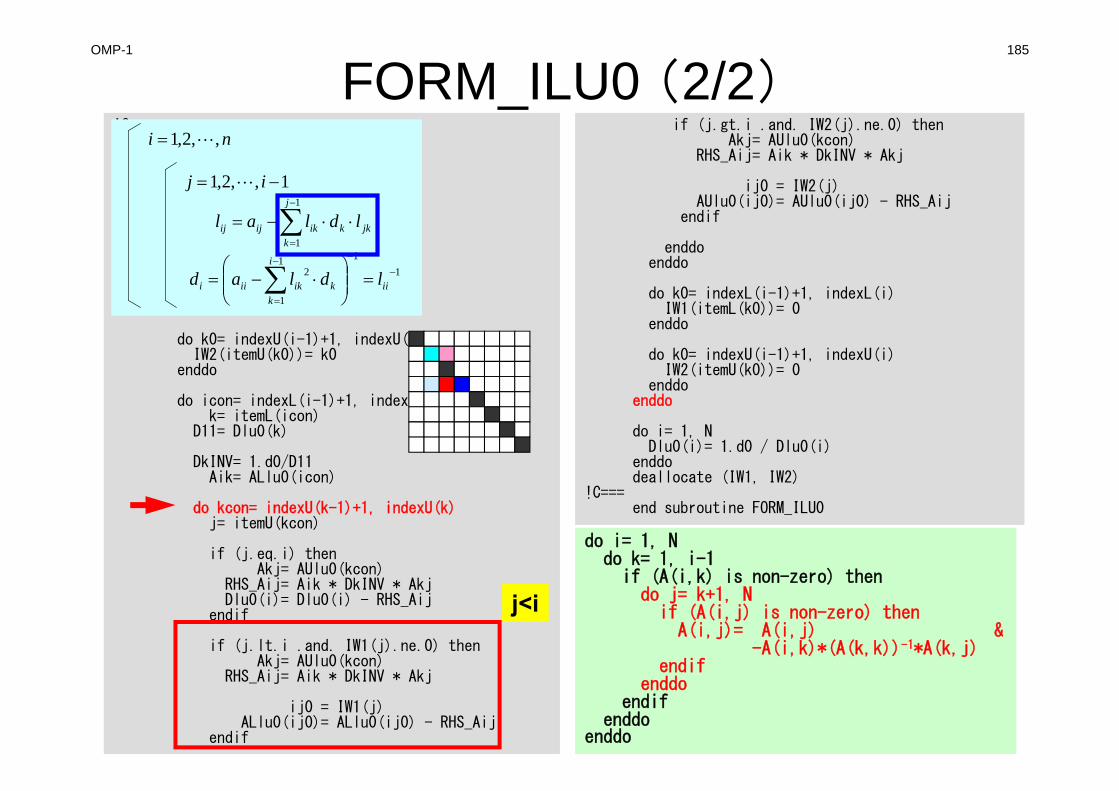
!C!C +----------------------+!C | ILU(0) factorization |!C +----------------------+!C===
allocate (IW1(N) , IW2(N))IW1=0IW2= 0
do i= 1, Ndo k0= indexL(i-1)+1, indexL(i)IW1(itemL(k0))= k0
enddo
do k0= indexU(i-1)+1, indexU(i)IW2(itemU(k0))= k0
enddo
do icon= indexL(i-1)+1, indexL(i)k= itemL(icon)
D11= Dlu0(k)
DkINV= 1.d0/D11Aik= ALlu0(icon)
do kcon= indexU(k-1)+1, indexU(k)j= itemU(kcon)
if (j.eq.i) thenAkj= AUlu0(kcon)
RHS_Aij= Aik * DkINV * AkjDlu0(i)= Dlu0(i) - RHS_Aij
endif
if (j.lt.i .and. IW1(j).ne.0) thenAkj= AUlu0(kcon)
RHS_Aij= Aik * DkINV * Akj
ij0 = IW1(j)ALlu0(ij0)= ALlu0(ij0) - RHS_Aij
endif
jkk
j
kikijij ldlal
1
1
ni ,,2,1
1,,2,1 ij
111
1
2
iik
i
kikiii ldlad
OMP-1 185
FORM_ILU0 (2/2)if (j.gt.i .and. IW2(j).ne.0) then
Akj= AUlu0(kcon)RHS_Aij= Aik * DkINV * Akj
ij0 = IW2(j)AUlu0(ij0)= AUlu0(ij0) - RHS_Aij
endif
enddoenddo
do k0= indexL(i-1)+1, indexL(i)IW1(itemL(k0))= 0
enddo
do k0= indexU(i-1)+1, indexU(i)IW2(itemU(k0))= 0
enddoenddo
do i= 1, NDlu0(i)= 1.d0 / Dlu0(i)
enddodeallocate (IW1, IW2)
!C===end subroutine FORM_ILU0
do i= 1, Ndo k= 1, i-1
if (A(i,k) is non-zero) thendo j= k+1, Nif (A(i,j) is non-zero) then
A(i,j)= A(i,j) &-A(i,k)*(A(k,k))-1*A(k,j)
endifenddo
endifenddo
enddo
j<i
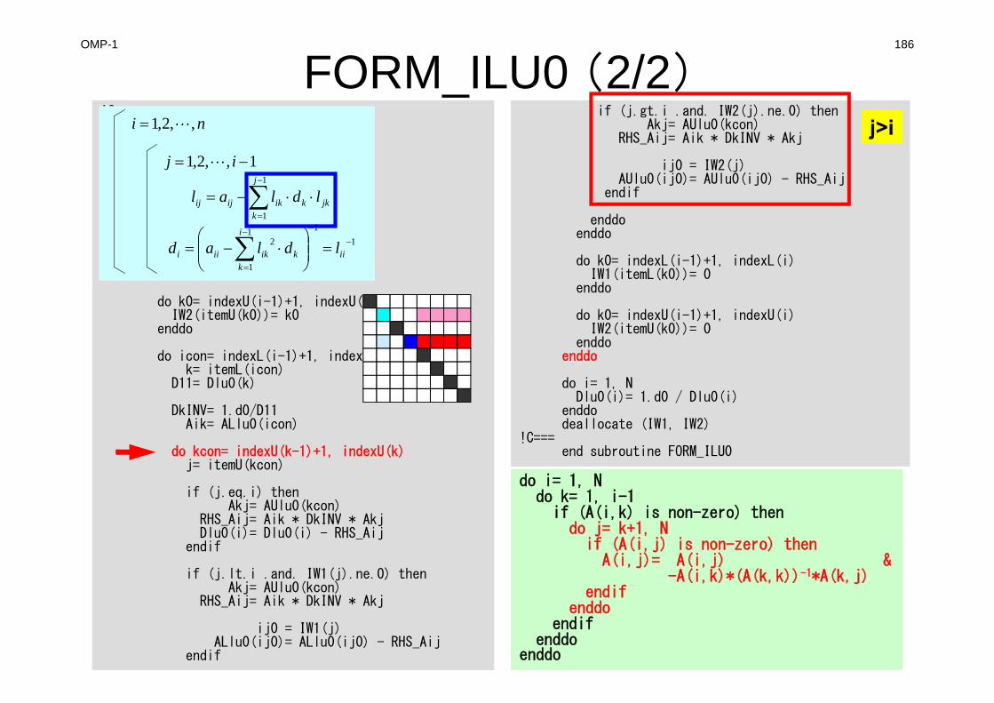
!C!C +----------------------+!C | ILU(0) factorization |!C +----------------------+!C===
allocate (IW1(N) , IW2(N))IW1=0IW2= 0
do i= 1, Ndo k0= indexL(i-1)+1, indexL(i)IW1(itemL(k0))= k0
enddo
do k0= indexU(i-1)+1, indexU(i)IW2(itemU(k0))= k0
enddo
do icon= indexL(i-1)+1, indexL(i)k= itemL(icon)
D11= Dlu0(k)
DkINV= 1.d0/D11Aik= ALlu0(icon)
do kcon= indexU(k-1)+1, indexU(k)j= itemU(kcon)
if (j.eq.i) thenAkj= AUlu0(kcon)
RHS_Aij= Aik * DkINV * AkjDlu0(i)= Dlu0(i) - RHS_Aij
endif
if (j.lt.i .and. IW1(j).ne.0) thenAkj= AUlu0(kcon)
RHS_Aij= Aik * DkINV * Akj
ij0 = IW1(j)ALlu0(ij0)= ALlu0(ij0) - RHS_Aij
endif
OMP-1 186
FORM_ILU0 (2/2)if (j.gt.i .and. IW2(j).ne.0) then
Akj= AUlu0(kcon)RHS_Aij= Aik * DkINV * Akj
ij0 = IW2(j)AUlu0(ij0)= AUlu0(ij0) - RHS_Aij
endif
enddoenddo
do k0= indexL(i-1)+1, indexL(i)IW1(itemL(k0))= 0
enddo
do k0= indexU(i-1)+1, indexU(i)IW2(itemU(k0))= 0
enddoenddo
do i= 1, NDlu0(i)= 1.d0 / Dlu0(i)
enddodeallocate (IW1, IW2)
!C===end subroutine FORM_ILU0
do i= 1, Ndo k= 1, i-1
if (A(i,k) is non-zero) thendo j= k+1, Nif (A(i,j) is non-zero) then
A(i,j)= A(i,j) &-A(i,k)*(A(k,k))-1*A(k,j)
endifenddo
endifenddo
enddo
j>i
jkk
j
kikijij ldlal
1
1
ni ,,2,1
1,,2,1 ij
111
1
2
iik
i
kikiii ldlad
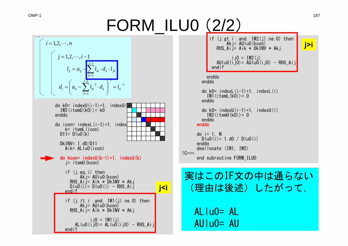
OMP-1 187
FORM_ILU0 (2/2)
実はこのIF文の中は通らない(理由は後述)したがって,
ALlu0= ALAUlu0= AU
!C!C +----------------------+!C | ILU(0) factorization |!C +----------------------+!C===
allocate (IW1(N) , IW2(N))IW1=0IW2= 0
do i= 1, Ndo k0= indexL(i-1)+1, indexL(i)IW1(itemL(k0))= k0
enddo
do k0= indexU(i-1)+1, indexU(i)IW2(itemU(k0))= k0
enddo
do icon= indexL(i-1)+1, indexL(i)k= itemL(icon)
D11= Dlu0(k)
DkINV= 1.d0/D11Aik= ALlu0(icon)
do kcon= indexU(k-1)+1, indexU(k)j= itemU(kcon)
if (j.eq.i) thenAkj= AUlu0(kcon)
RHS_Aij= Aik * DkINV * AkjDlu0(i)= Dlu0(i) - RHS_Aij
endif
if (j.lt.i .and. IW1(j).ne.0) thenAkj= AUlu0(kcon)
RHS_Aij= Aik * DkINV * Akj
ij0 = IW1(j)ALlu0(ij0)= ALlu0(ij0) - RHS_Aij
endif
if (j.gt.i .and. IW2(j).ne.0) thenAkj= AUlu0(kcon)
RHS_Aij= Aik * DkINV * Akj
ij0 = IW2(j)AUlu0(ij0)= AUlu0(ij0) - RHS_Aij
endif
enddoenddo
do k0= indexL(i-1)+1, indexL(i)IW1(itemL(k0))= 0
enddo
do k0= indexU(i-1)+1, indexU(i)IW2(itemU(k0))= 0
enddoenddo
do i= 1, NDlu0(i)= 1.d0 / Dlu0(i)
enddodeallocate (IW1, IW2)
!C===end subroutine FORM_ILU0
j>i
jkk
j
kikijij ldlal
1
1
ni ,,2,1
1,,2,1 ij
111
1
2
iik
i
kikiii ldlad
j<i
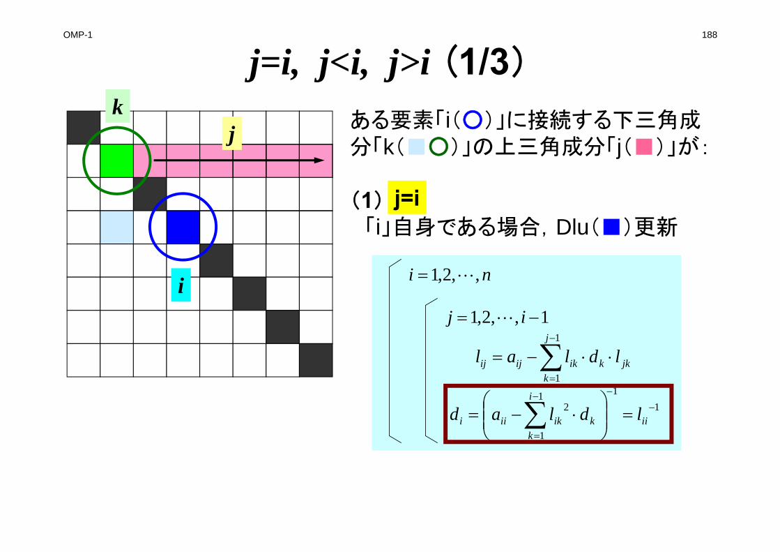
OMP-1 188
j=i, j<i, j>i (1/3)
i
kある要素「i(○)」に接続する下三角成分「k(■○)」の上三角成分「j(■)」が:
(1)「i」自身である場合,Dlu(■)更新
j=i
j
jkk
j
kikijij ldlal
1
1
ni ,,2,1
1,,2,1 ij
111
1
2
iik
i
kikiii ldlad
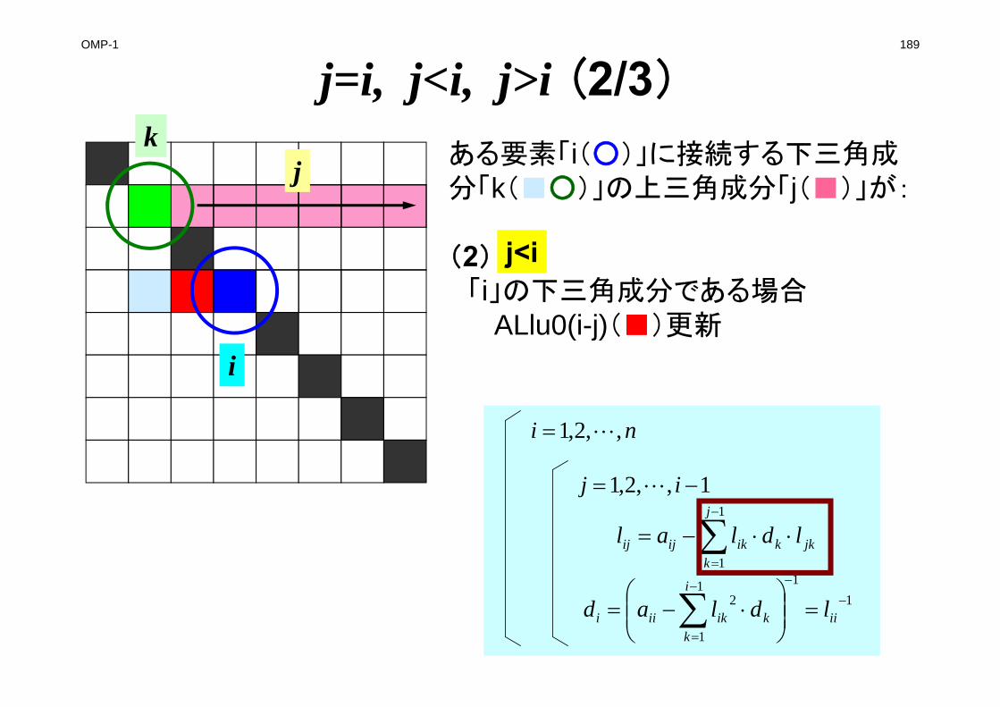
OMP-1 189
j=i, j<i, j>i (2/3)
i
kある要素「i(○)」に接続する下三角成分「k(■○)」の上三角成分「j(■)」が:
(2)「i」の下三角成分である場合
ALlu0(i-j)(■)更新
j<i
j
jkk
j
kikijij ldlal
1
1
ni ,,2,1
1,,2,1 ij
111
1
2
iik
i
kikiii ldlad
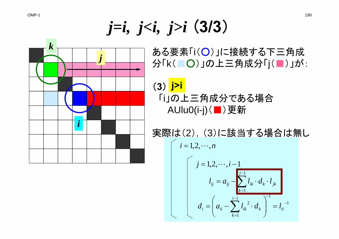
OMP-1 190
j=i, j<i, j>i (3/3)
i
kある要素「i(○)」に接続する下三角成分「k(■○)」の上三角成分「j(■)」が:
(3)「i」の上三角成分である場合
AUlu0(i-j)(■)更新
実際は(2),(3)に該当する場合は無し
j>i
j
jkk
j
kikijij ldlal
1
1
ni ,,2,1
1,,2,1 ij
111
1
2
iik
i
kikiii ldlad
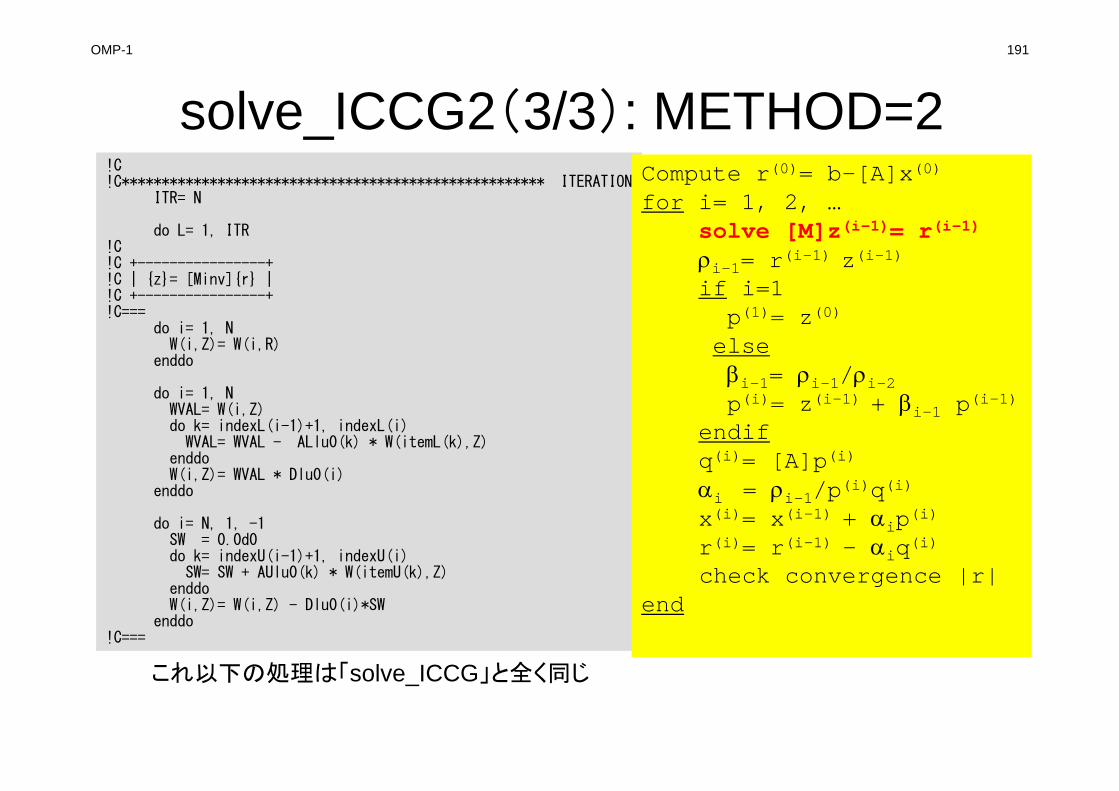
OMP-1 191
solve_ICCG2(3/3): METHOD=2!C!C***************************************************** ITERATION
ITR= N
do L= 1, ITR!C!C +----------------+!C | {z}= [Minv]{r} |!C +----------------+!C===
do i= 1, NW(i,Z)= W(i,R)
enddo
do i= 1, NWVAL= W(i,Z)do k= indexL(i-1)+1, indexL(i)WVAL= WVAL - ALlu0(k) * W(itemL(k),Z)
enddoW(i,Z)= WVAL * Dlu0(i)
enddo
do i= N, 1, -1SW = 0.0d0do k= indexU(i-1)+1, indexU(i)SW= SW + AUlu0(k) * W(itemU(k),Z)
enddoW(i,Z)= W(i,Z) - Dlu0(i)*SW
enddo!C===
これ以下の処理は「solve_ICCG」と全く同じ
Compute r(0)= b-[A]x(0)
for i= 1, 2, …solve [M]z(i-1)= r(i-1)
i-1= r(i-1) z(i-1)if i=1p(1)= z(0)
elsei-1= i-1/i-2p(i)= z(i-1) + i-1 p(i-1)
endifq(i)= [A]p(i)
i = i-1/p(i)q(i)x(i)= x(i-1) + ip(i)r(i)= r(i-1) - iq(i)check convergence |r|
end
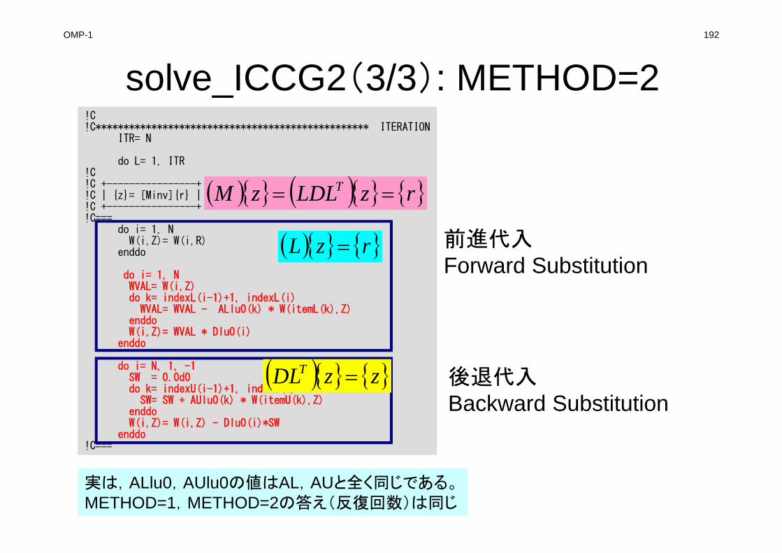
OMP-1 192
solve_ICCG2(3/3): METHOD=2!C!C************************************************* ITERATION
ITR= N
do L= 1, ITR!C!C +----------------+!C | {z}= [Minv]{r} |!C +----------------+!C===
do i= 1, NW(i,Z)= W(i,R)
enddo
do i= 1, NWVAL= W(i,Z)do k= indexL(i-1)+1, indexL(i)WVAL= WVAL - ALlu0(k) * W(itemL(k),Z)
enddoW(i,Z)= WVAL * Dlu0(i)
enddo
do i= N, 1, -1SW = 0.0d0do k= indexU(i-1)+1, indexU(i)SW= SW + AUlu0(k) * W(itemU(k),Z)
enddoW(i,Z)= W(i,Z) - Dlu0(i)*SW
enddo!C===
実は,ALlu0,AUlu0の値はAL,AUと全く同じである。METHOD=1,METHOD=2の答え(反復回数)は同じ
rzLDLzM T
rzL
zzDLT
前進代入Forward Substitution
後退代入Backward Substitution
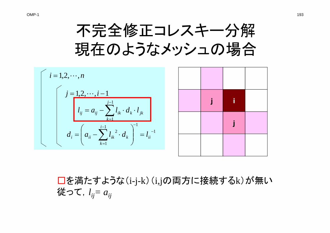
OMP-1 193
不完全修正コレスキー分解現在のようなメッシュの場合
jkk
j
kikijij ldlal
1
1
ni ,,2,1
1,,2,1 ij
111
1
2
iik
i
kikiii ldlad
j i
j
□を満たすような(i-j-k)(i,jの両方に接続するk)が無い従って,lij= aij
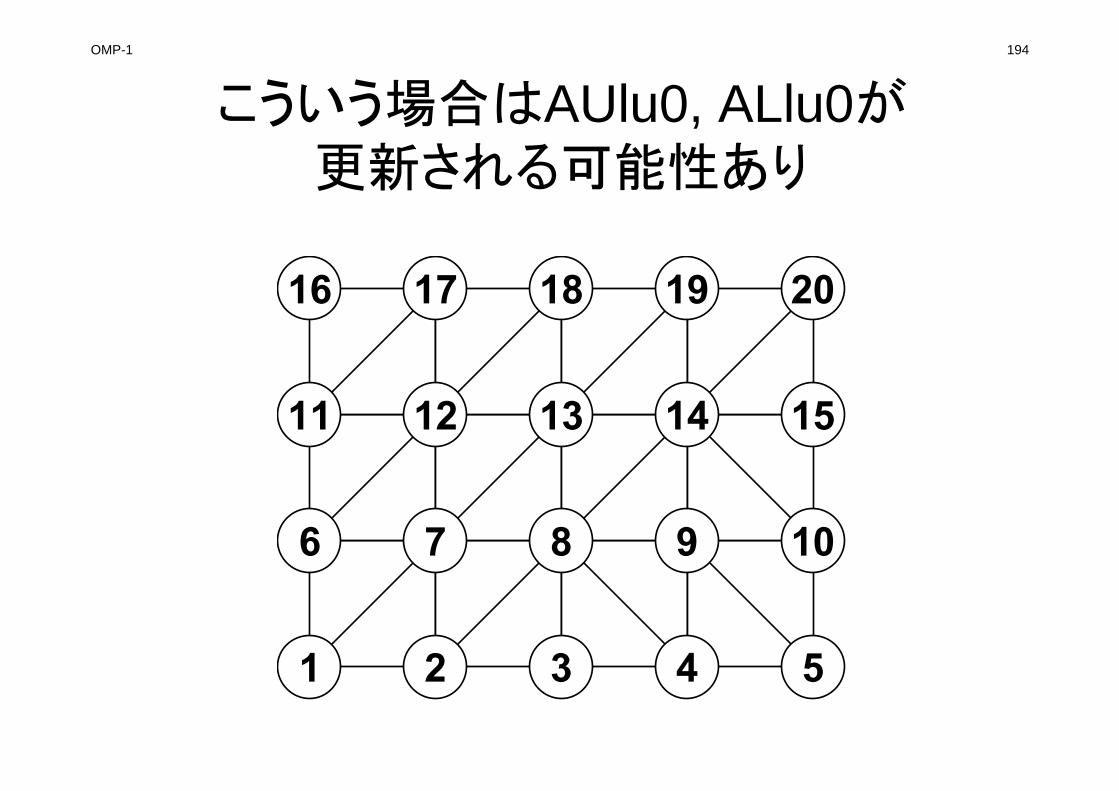
OMP-1 194
こういう場合はAUlu0, ALlu0が更新される可能性あり
1 2 3 4 5
6 7 8 9 10
11 12 13 14 15
16 17 18 19 20
195
• 背景
– 有限体積法
– 前処理付反復法
• ICCG法によるポアソン方程式法ソルバーについて
– 実行方法• データ構造
– プログラムの説明• 初期化
• 係数マトリクス生成
• ICCG法
• OpenMP
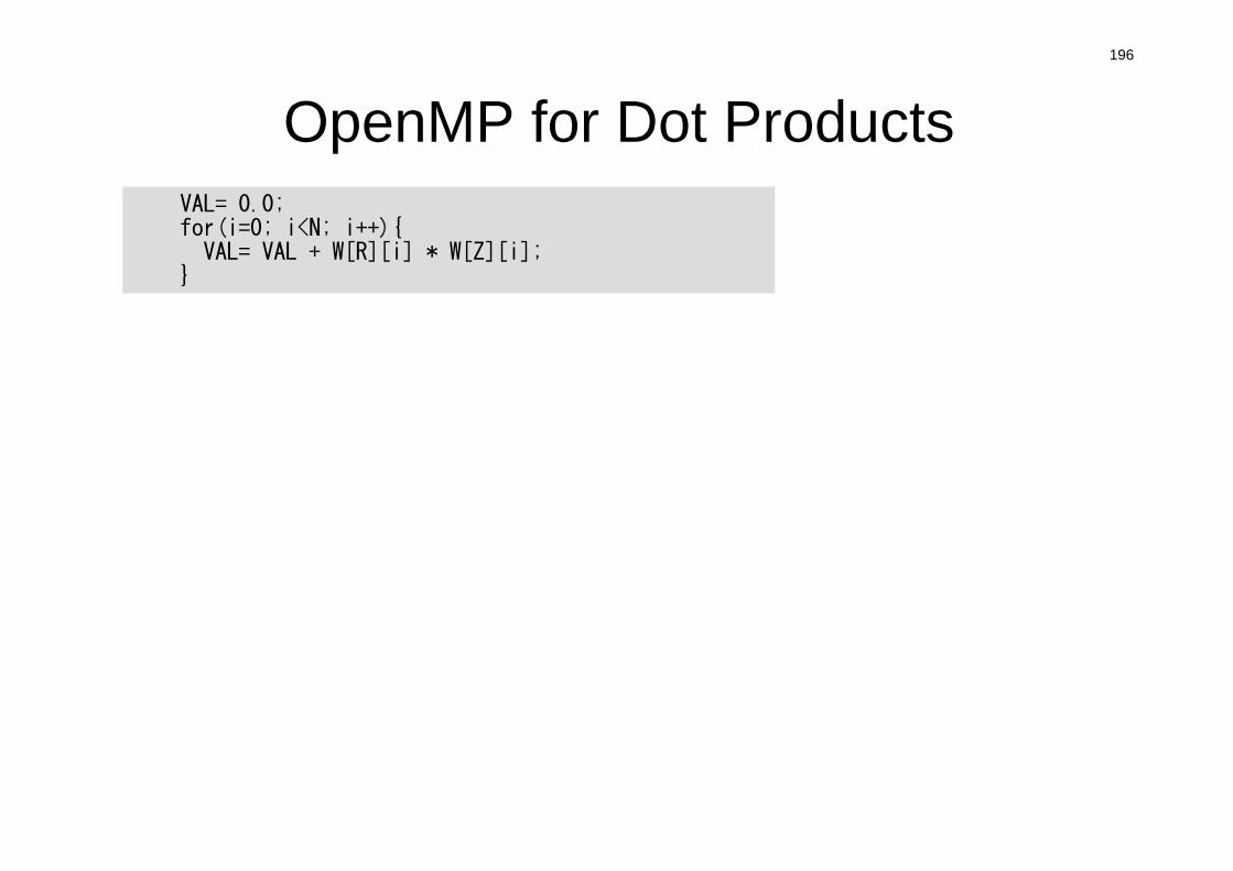
196
OpenMP for Dot ProductsVAL= 0.0;for(i=0; i<N; i++){VAL= VAL + W[R][i] * W[Z][i];
}
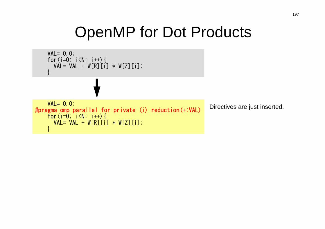
197
OpenMP for Dot Products
VAL= 0.0;#pragma omp parallel for private (i) reduction(+:VAL)
for(i=0; i<N; i++){VAL= VAL + W[R][i] * W[Z][i];
}
Directives are just inserted.
VAL= 0.0;for(i=0; i<N; i++){VAL= VAL + W[R][i] * W[Z][i];
}
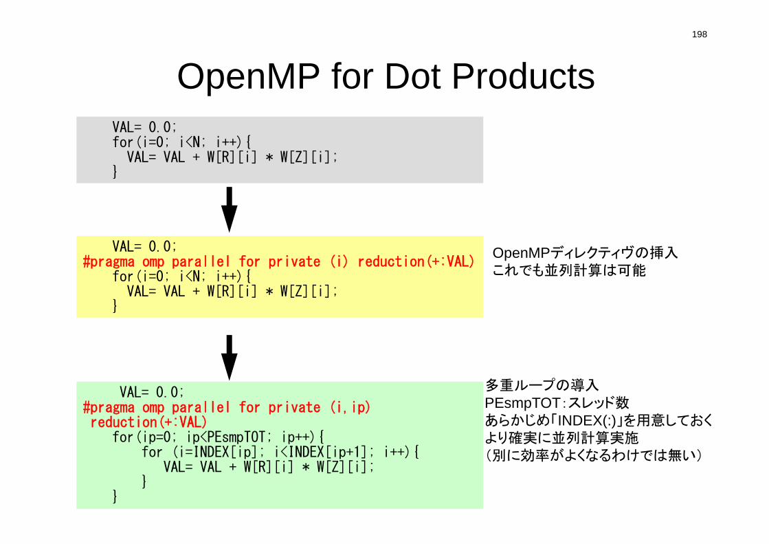
198
OpenMP for Dot Products
VAL= 0.0;#pragma omp parallel for private (i,ip) reduction(+:VAL)
for(ip=0; ip<PEsmpTOT; ip++){for (i=INDEX[ip]; i<INDEX[ip+1]; i++){
VAL= VAL + W[R][i] * W[Z][i]; }
}
VAL= 0.0;for(i=0; i<N; i++){VAL= VAL + W[R][i] * W[Z][i];
}
VAL= 0.0;#pragma omp parallel for private (i) reduction(+:VAL)
for(i=0; i<N; i++){VAL= VAL + W[R][i] * W[Z][i];
}
OpenMPディレクティヴの挿入これでも並列計算は可能
多重ループの導入PEsmpTOT:スレッド数あらかじめ「INDEX(:)」を用意しておくより確実に並列計算実施(別に効率がよくなるわけでは無い)
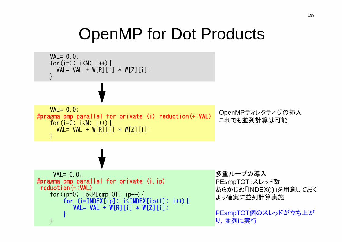
199
OpenMP for Dot Products
VAL= 0.0;#pragma omp parallel for private (i,ip) reduction(+:VAL)
for(ip=0; ip<PEsmpTOT; ip++){for (i=INDEX[ip]; i<INDEX[ip+1]; i++){
VAL= VAL + W[R][i] * W[Z][i]; }
}
VAL= 0.0;for(i=0; i<N; i++){VAL= VAL + W[R][i] * W[Z][i];
}
VAL= 0.0;#pragma omp parallel for private (i) reduction(+:VAL)
for(i=0; i<N; i++){VAL= VAL + W[R][i] * W[Z][i];
}
OpenMPディレクティヴの挿入これでも並列計算は可能
多重ループの導入PEsmpTOT:スレッド数あらかじめ「INDEX(:)」を用意しておくより確実に並列計算実施
PEsmpTOT個のスレッドが立ち上がり,並列に実行
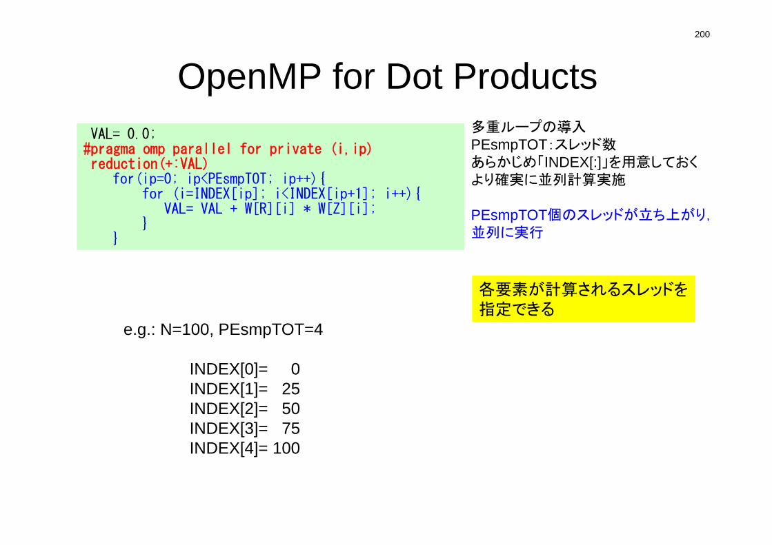
200
OpenMP for Dot ProductsVAL= 0.0;
#pragma omp parallel for private (i,ip) reduction(+:VAL)
for(ip=0; ip<PEsmpTOT; ip++){for (i=INDEX[ip]; i<INDEX[ip+1]; i++){
VAL= VAL + W[R][i] * W[Z][i]; }
}
e.g.: N=100, PEsmpTOT=4
INDEX[0]= 0INDEX[1]= 25INDEX[2]= 50INDEX[3]= 75INDEX[4]= 100
多重ループの導入PEsmpTOT:スレッド数あらかじめ「INDEX[:]」を用意しておくより確実に並列計算実施
PEsmpTOT個のスレッドが立ち上がり,並列に実行
各要素が計算されるスレッドを指定できる
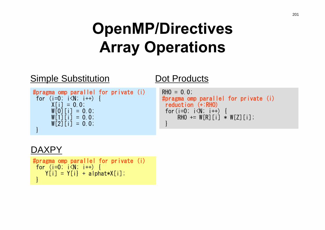
201
OpenMP/DirectivesArray Operations
#pragma omp parallel for private (i)for (i=0; i<N; i++) {
X[i] = 0.0;W[0][i] = 0.0;W[1][i] = 0.0;W[2][i] = 0.0;
}
RHO = 0.0;#pragma omp parallel for private (i)reduction (+:RHO)for(i=0; i<N; i++) {
RHO += W[R][i] * W[Z][i];}
Simple Substitution Dot Products
#pragma omp parallel for private (i)for (i=0; i<N; i++) {
Y[i] = Y[i} + alphat*X[i]; }
DAXPY
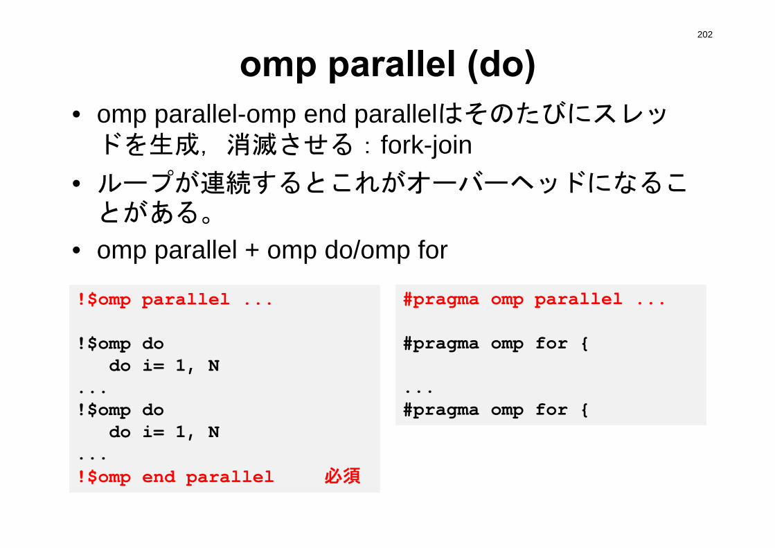
202
omp parallel (do)• omp parallel-omp end parallelはそのたびにスレッドを生成,消滅させる:fork-join
• ループが連続するとこれがオーバーヘッドになることがある。
• omp parallel + omp do/omp for
#pragma omp parallel ...
#pragma omp for {
...#pragma omp for {
!$omp parallel ...
!$omp dodo i= 1, N
...!$omp do
do i= 1, N...!$omp end parallel 必須
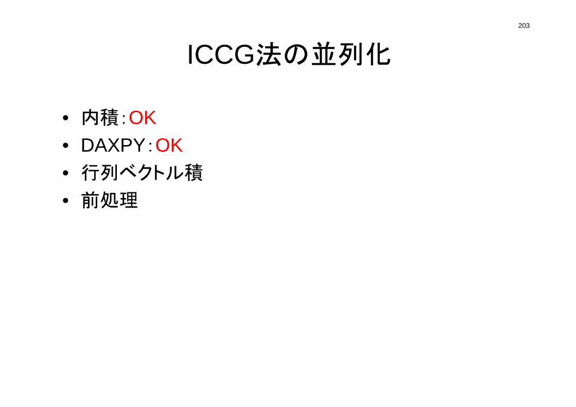
203
ICCG法の並列化
• 内積:OK• DAXPY:OK• 行列ベクトル積
• 前処理
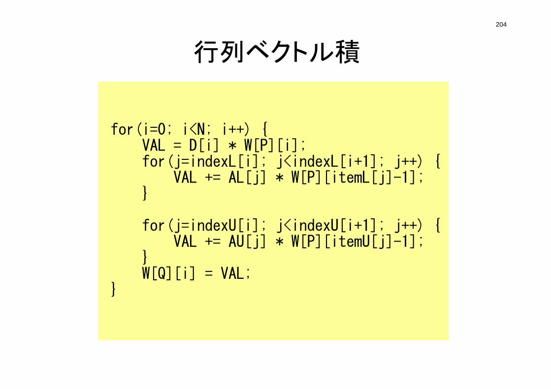
204
行列ベクトル積
for(i=0; i<N; i++) {VAL = D[i] * W[P][i];for(j=indexL[i]; j<indexL[i+1]; j++) {
VAL += AL[j] * W[P][itemL[j]-1];}
for(j=indexU[i]; j<indexU[i+1]; j++) {VAL += AU[j] * W[P][itemU[j]-1];
}W[Q][i] = VAL;
}
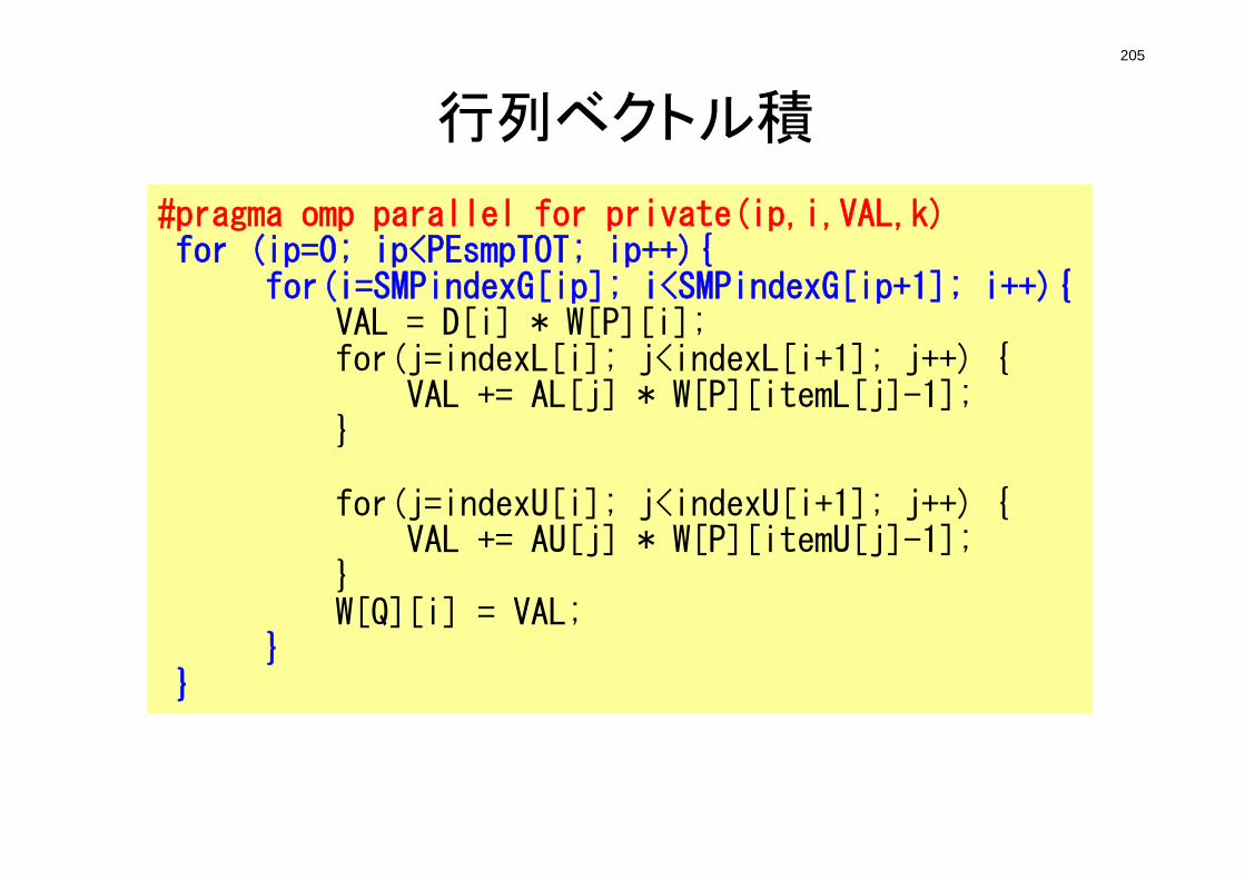
205
行列ベクトル積
#pragma omp parallel for private(ip,i,VAL,k)for (ip=0; ip<PEsmpTOT; ip++){
for(i=SMPindexG[ip]; i<SMPindexG[ip+1]; i++){VAL = D[i] * W[P][i];for(j=indexL[i]; j<indexL[i+1]; j++) {
VAL += AL[j] * W[P][itemL[j]-1];}
for(j=indexU[i]; j<indexU[i+1]; j++) {VAL += AU[j] * W[P][itemU[j]-1];
}W[Q][i] = VAL;
}}
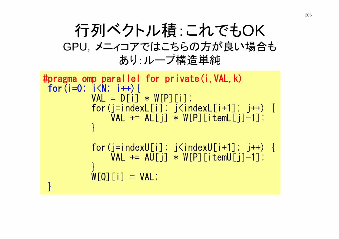
206
行列ベクトル積:これでもOKGPU,メニィコアではこちらの方が良い場合も
あり:ループ構造単純
#pragma omp parallel for private(i,VAL,k)for(i=0; i<N; i++){
VAL = D[i] * W[P][i];for(j=indexL[i]; j<indexL[i+1]; j++) {
VAL += AL[j] * W[P][itemL[j]-1];}
for(j=indexU[i]; j<indexU[i+1]; j++) {VAL += AU[j] * W[P][itemU[j]-1];
}W[Q][i] = VAL;
}
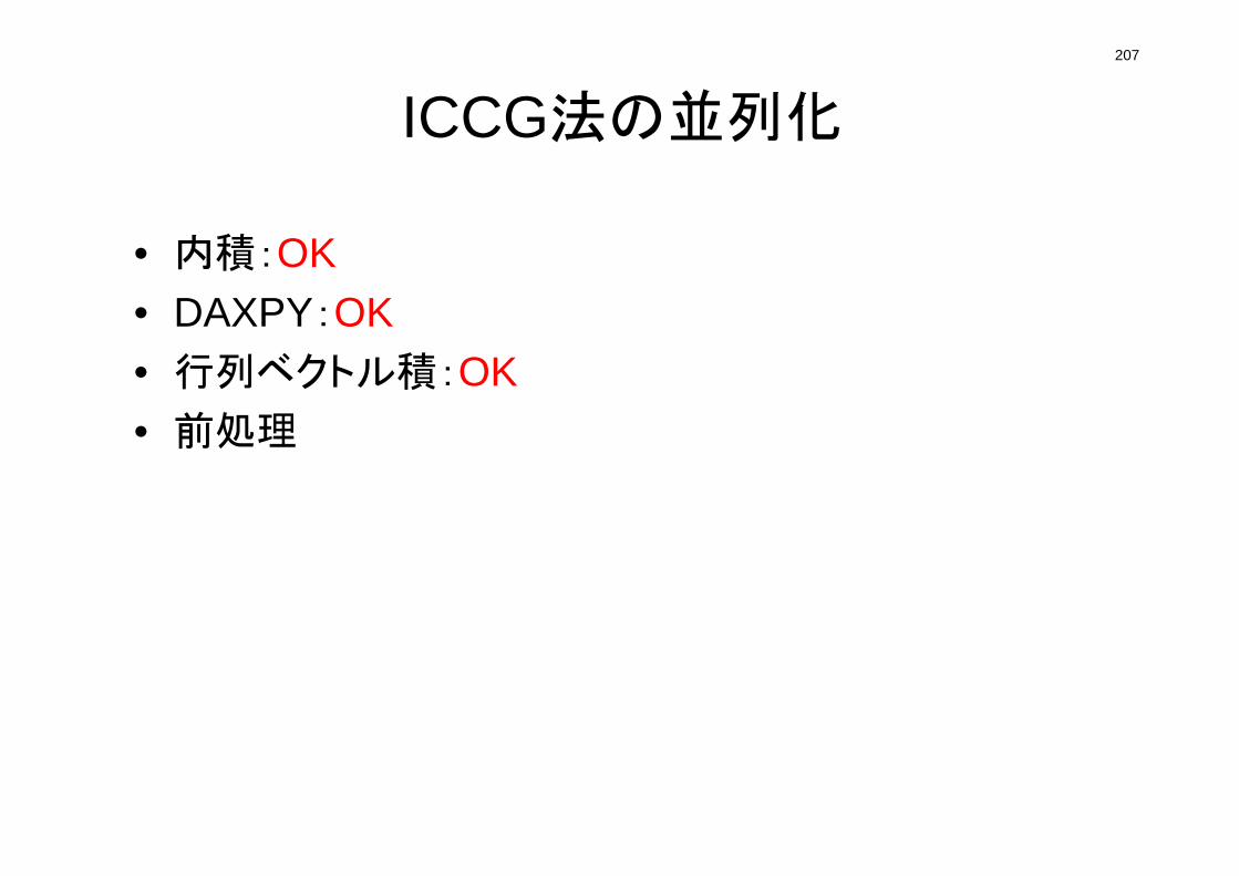
207
ICCG法の並列化
• 内積:OK• DAXPY:OK• 行列ベクトル積:OK• 前処理
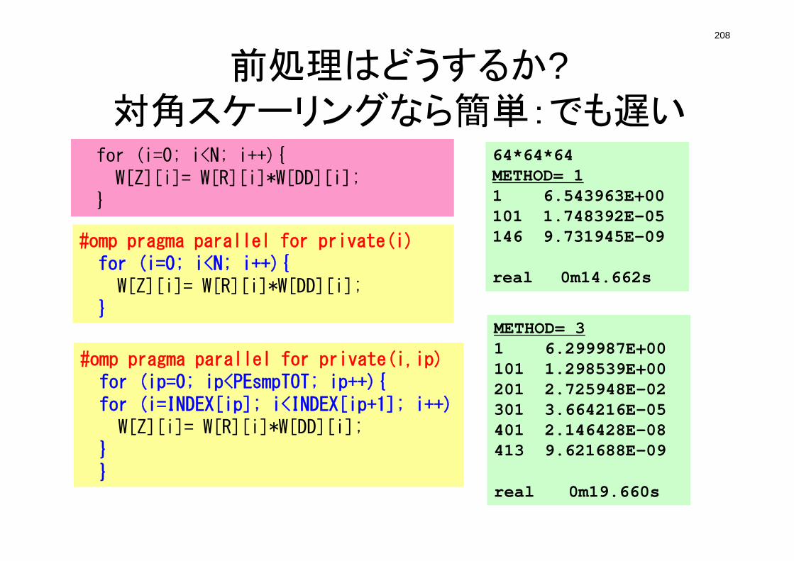
208
前処理はどうするか?対角スケーリングなら簡単:でも遅い
for (i=0; i<N; i++){W[Z][i]= W[R][i]*W[DD][i];
}
#omp pragma parallel for private(i)for (i=0; i<N; i++){W[Z][i]= W[R][i]*W[DD][i];
}
64*64*64METHOD= 11 6.543963E+00101 1.748392E-05146 9.731945E-09
real 0m14.662s
METHOD= 31 6.299987E+00101 1.298539E+00201 2.725948E-02301 3.664216E-05401 2.146428E-08413 9.621688E-09
real 0m19.660s
#omp pragma parallel for private(i,ip)for (ip=0; ip<PEsmpTOT; ip++){for (i=INDEX[ip]; i<INDEX[ip+1]; i++)W[Z][i]= W[R][i]*W[DD][i];
}}
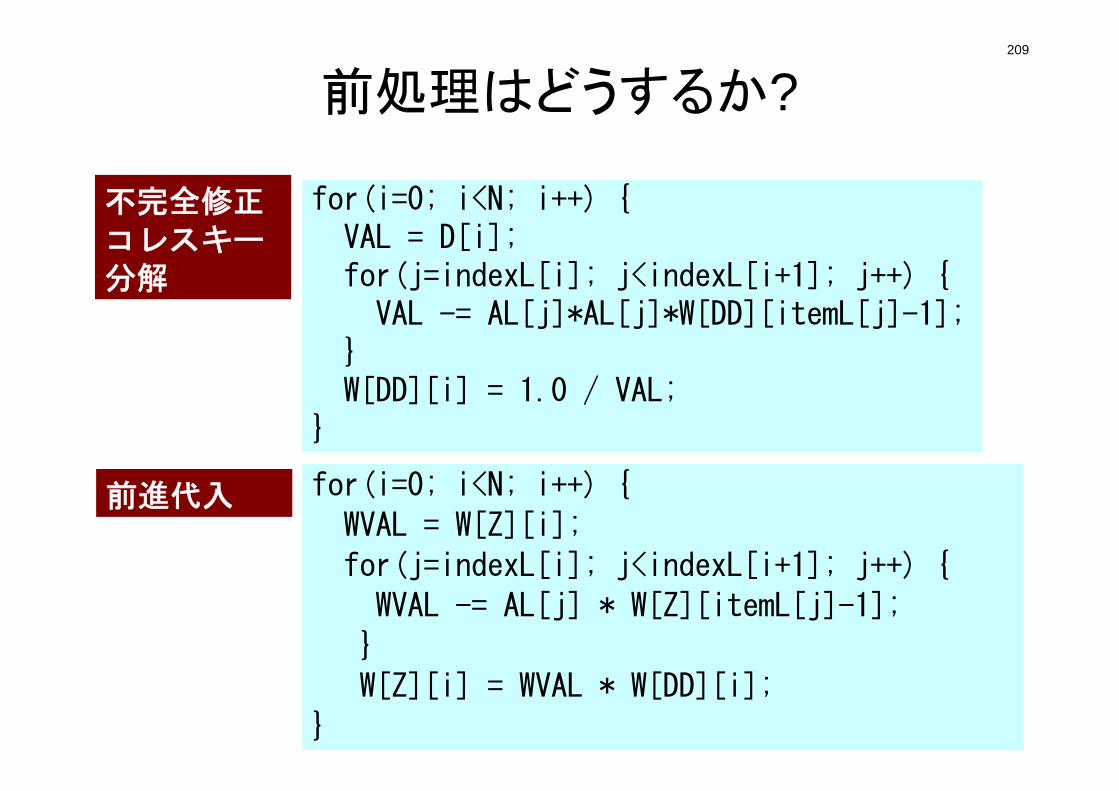
209
前処理はどうするか?
for(i=0; i<N; i++) {VAL = D[i];for(j=indexL[i]; j<indexL[i+1]; j++) {VAL -= AL[j]*AL[j]*W[DD][itemL[j]-1];
}W[DD][i] = 1.0 / VAL;
}
for(i=0; i<N; i++) {
WVAL = W[Z][i];
for(j=indexL[i]; j<indexL[i+1]; j++) {
WVAL -= AL[j] * W[Z][itemL[j]-1];
}
W[Z][i] = WVAL * W[DD][i];
}
不完全修正コレスキー分解
前進代入
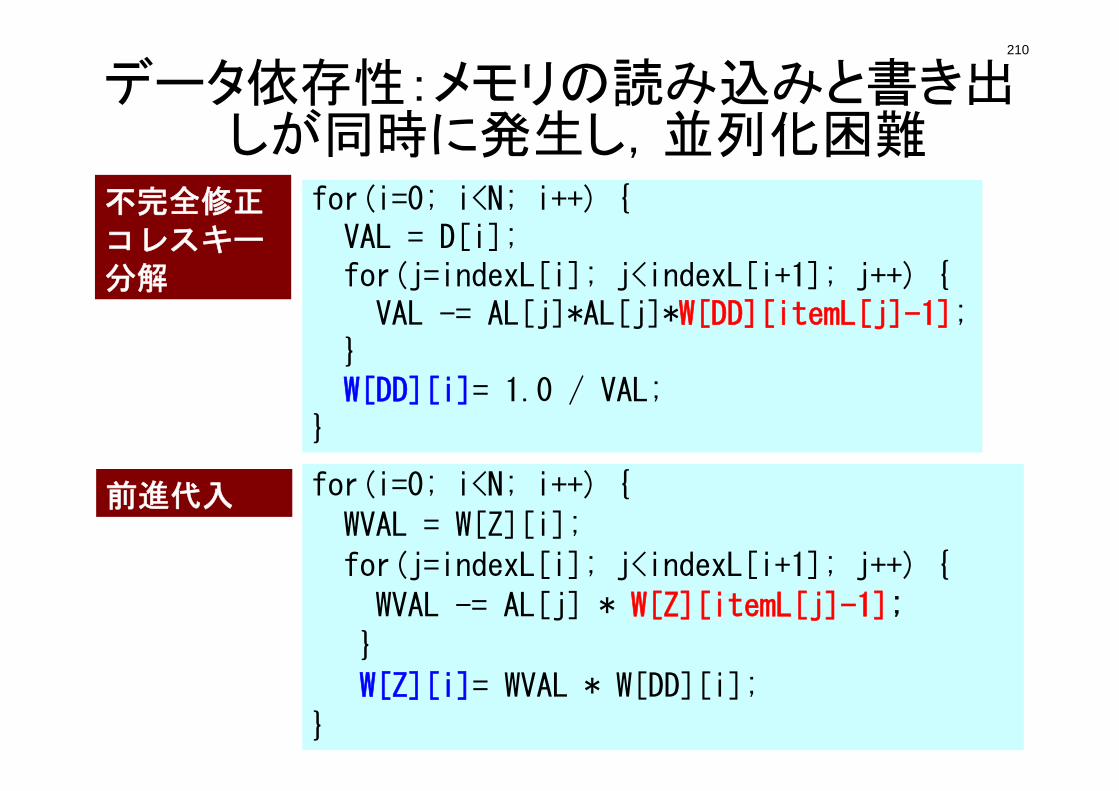
210
データ依存性:メモリの読み込みと書き出しが同時に発生し,並列化困難
for(i=0; i<N; i++) {VAL = D[i];for(j=indexL[i]; j<indexL[i+1]; j++) {VAL -= AL[j]*AL[j]*W[DD][itemL[j]-1];
}W[DD][i]= 1.0 / VAL;
}
for(i=0; i<N; i++) {
WVAL = W[Z][i];
for(j=indexL[i]; j<indexL[i+1]; j++) {
WVAL -= AL[j] * W[Z][itemL[j]-1];
}
W[Z][i]= WVAL * W[DD][i];
}
不完全修正コレスキー分解
前進代入
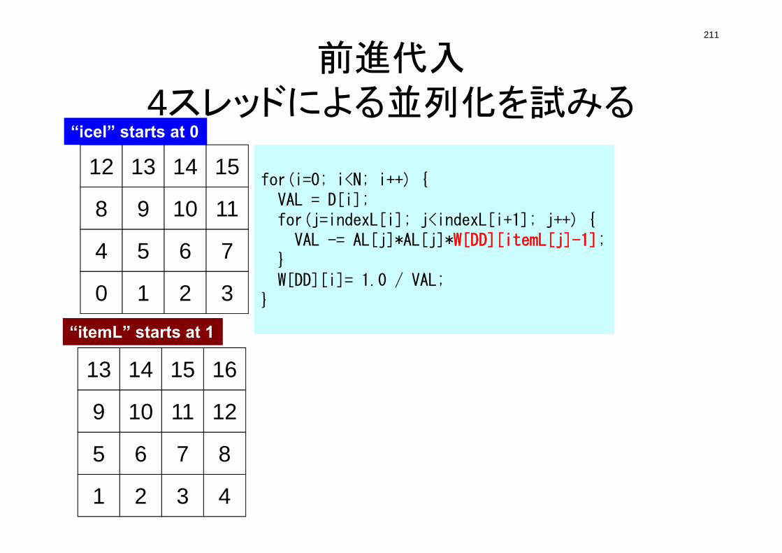
211
前進代入4スレッドによる並列化を試みる
0 1 2 3
4 5 6 7
8 9 10 11
12 13 14 15for(i=0; i<N; i++) {VAL = D[i];for(j=indexL[i]; j<indexL[i+1]; j++) {VAL -= AL[j]*AL[j]*W[DD][itemL[j]-1];
}W[DD][i]= 1.0 / VAL;
}
1 2 3 4
5 6 7 8
9 10 11 12
13 14 15 16
“icel” starts at 0
“itemL” starts at 1
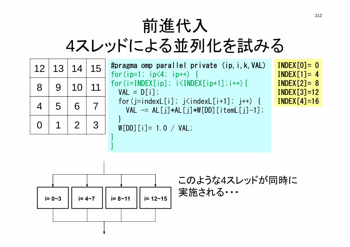
212
前進代入4スレッドによる並列化を試みる
INDEX[0]= 0INDEX[1]= 4INDEX[2]= 8INDEX[3]=12INDEX[4]=16
do i=1,4…enddo
do i=5,8…enddo
do i=9,12…enddo
do i=13,16…enddo
do i=1,4…enddo
do i=5,8…enddo
do i=9,12…enddo
do i=13,16…enddo
#pragma omp parallel private (ip,i,k,VAL)for(ip=1; ip<4; ip++) {for(i=INDEX[ip]; i<INDEX[ip+1];i++){VAL = D[i];for(j=indexL[i]; j<indexL[i+1]; j++) {VAL -= AL[j]*AL[j]*W[DD][itemL[j]-1];
}W[DD][i]= 1.0 / VAL;
}}
0 1 2 3
4 5 6 7
8 9 10 11
12 13 14 15
i= 0~3 i= 4~7 i= 8~11 i= 12~15
このような4スレッドが同時に実施される・・・
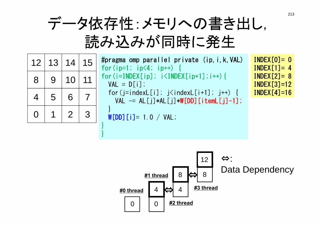
213
データ依存性:メモリへの書き出し,読み込みが同時に発生
1 1
5 5
9 9
13
⇔
⇔1 1
5
1
5 5
9
5
9 9
13
9
13
⇔
⇔
⇔:Data Dependency
#0 thread
#1 thread
#2 thread
#3 thread
INDEX[0]= 0INDEX[1]= 4INDEX[2]= 8INDEX[3]=12INDEX[4]=16
#pragma omp parallel private (ip,i,k,VAL)for(ip=1; ip<4; ip++) {for(i=INDEX[ip]; i<INDEX[ip+1];i++){VAL = D[i];for(j=indexL[i]; j<indexL[i+1]; j++) {VAL -= AL[j]*AL[j]*W[DD][itemL[j]-1];
}W[DD][i]= 1.0 / VAL;
}}
0 1 2 3
4 5 6 7
8 9 10 11
12 13 14 15
0 0
4 4
8 8
12
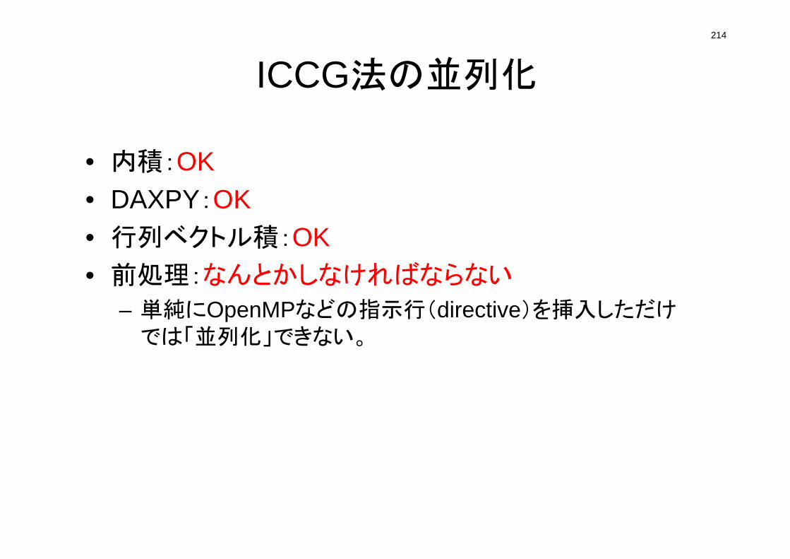
214
ICCG法の並列化
• 内積:OK• DAXPY:OK• 行列ベクトル積:OK• 前処理:なんとかしなければならない
– 単純にOpenMPなどの指示行(directive)を挿入しただけでは「並列化」できない。