Embed Size (px)
Citation preview
선형회귀분석regression analysis
Chapter 9
2017/5/8

9.1 머리말 (Intro)
• Sir Francis Galton (1822-1911)’s studies on genetics
• Heights of parents’ and children: 부모의 신장에 비해 2세의 신장이 일반 평균치에 복귀(revert to the pop mean)하는특성을 발견하였다.
• 복귀(revert)는 회귀(regression)로 표현하기로 하였다.
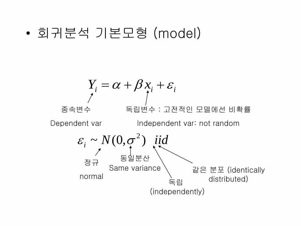
• 회귀분석 기본모형 (model)
i i iY x
종속변수
Dependent var
독립변수 : 고전적인 모델에선 비확률
Independent var: not random
2~ (0, )i N iid
정규
normal
동일분산
Same variance 같은 분포 (identically distributed)독립
(independently)
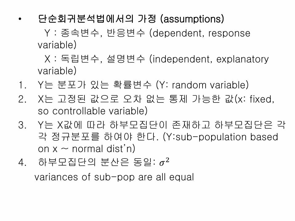
• 단순회귀분석법에서의 가정 (assumptions)
Y : 종속변수, 반응변수 (dependent, response variable)
X : 독립변수, 설명변수 (independent, explanatory variable)
1. Y는 분포가 있는 확률변수 (Y: random variable)
2. X는 고정된 값으로 오차 없는 통제 가능한 값(x: fixed, so controllable variable)
3. Y는 X값에 따라 하부모집단이 존재하고 하부모집단은 각각 정규분포를 하여야 한다. (Y:sub-population based on x ~ normal dist’n)
4. 하부모집단의 분산은 동일: 𝜎2
variances of sub-pop are all equal
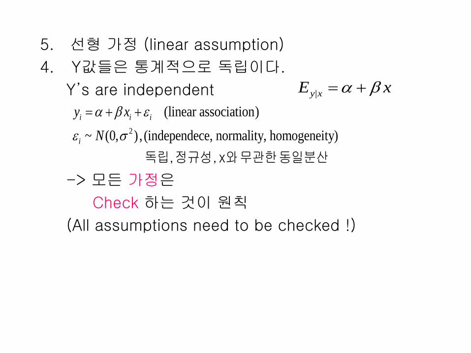
5. 선형 가정 (linear assumption)
4. Y값들은 통계적으로 독립이다.
Y’s are independent
-> 모든 가정은
Check 하는 것이 원칙
(All assumptions need to be checked !)
|y xE x
2
(linear association)
~ (0, ) , (independece, normality, homogeneity)
i i i
i
y x
N
독립, 정규성 , x와 무관한 동일분산
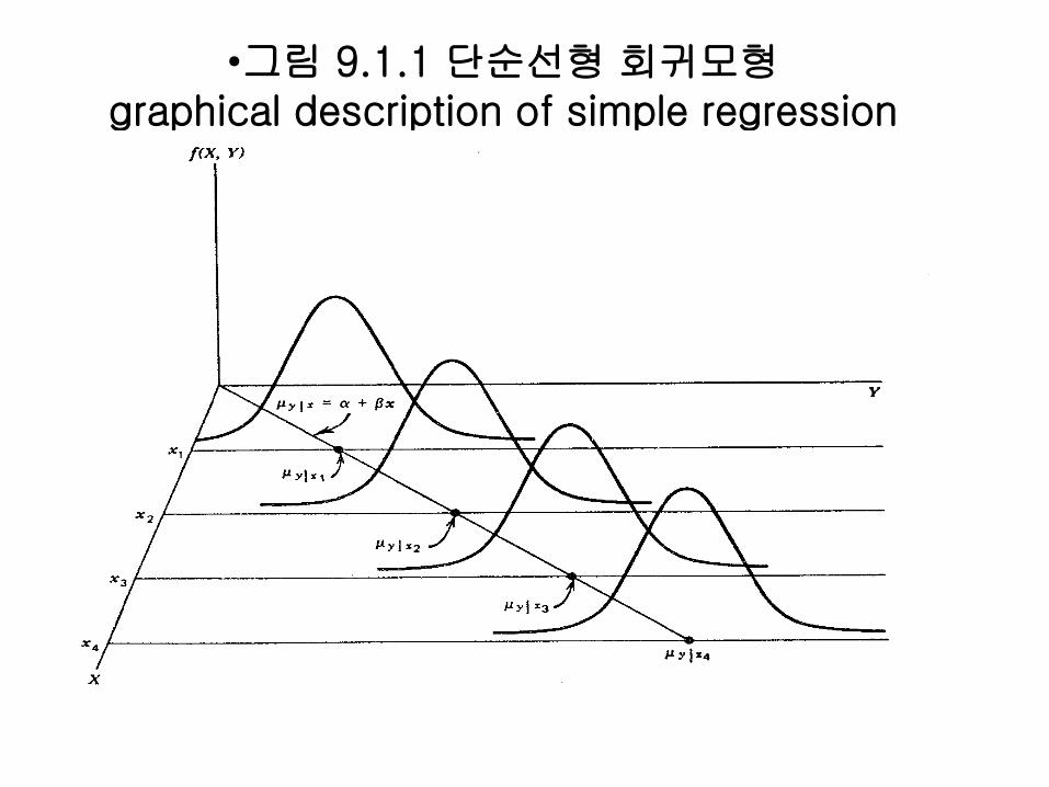
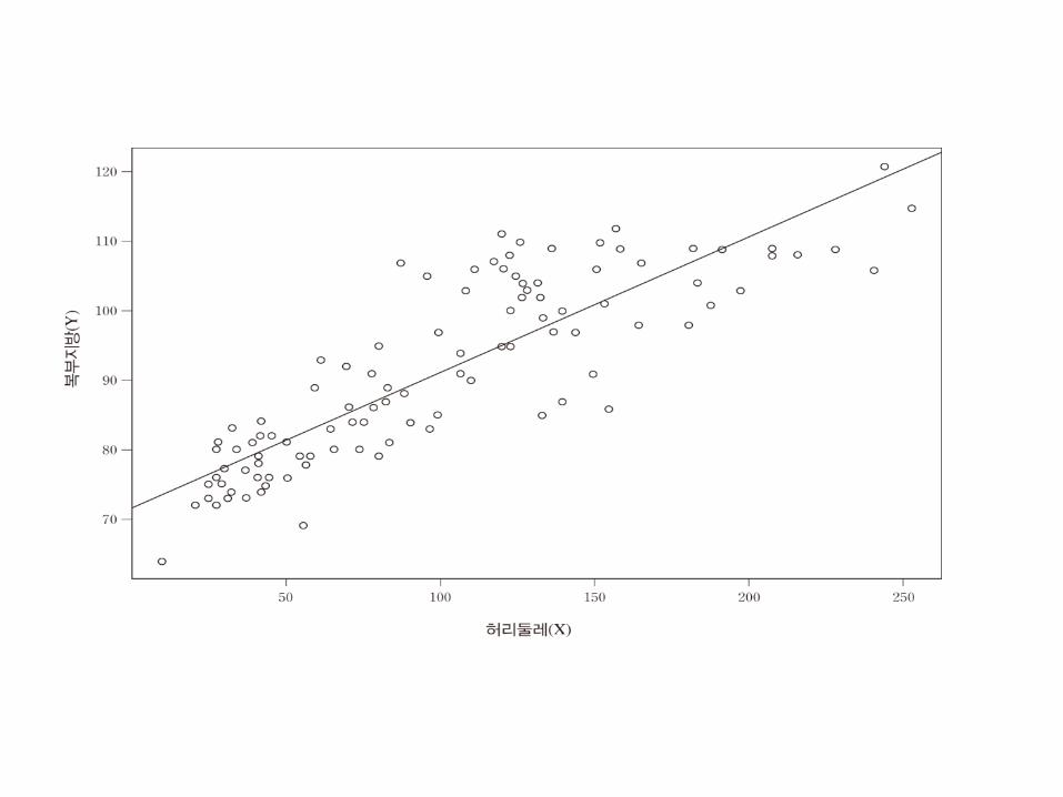
•그림 9.1.1 단순선형 회귀모형graphical description of simple regression
9.2 표본회귀방정식simple linear regression
Ex 9.2.1 복부 내 AT의 양을 이용하여 심혈관 질환의 위험성을 평가할 수있다고 알려져 있다. 그러나 복부 지방 조직의 양을 정확하고 신뢰도 있게측정할 수 있는 유일한 기술인 전산화 단층 촬영(CT)은 비싸고 검진받기에불편하다. 또한 전산화 단층 촬영기계는 비싸기 때문에 대형 병원에 있는의사들만이 사용할 수 있다. 이러한 이유로 한 연구자는 허리둘레를이용하여 심복부 지방 조직의 양을 예측할 수 있는 방정식을 추론하기위하여 표본을 수집하였다. 표본은 대사성 질환이 없는 18세에서 42세의남성으로, 표본의 CT로부터 얻은 복부 지방 조직과 허리 둘레 관측값은 [표9.2.1]을 참고하여라.
(Abdominal fat) = a + b* (Waist circumference)
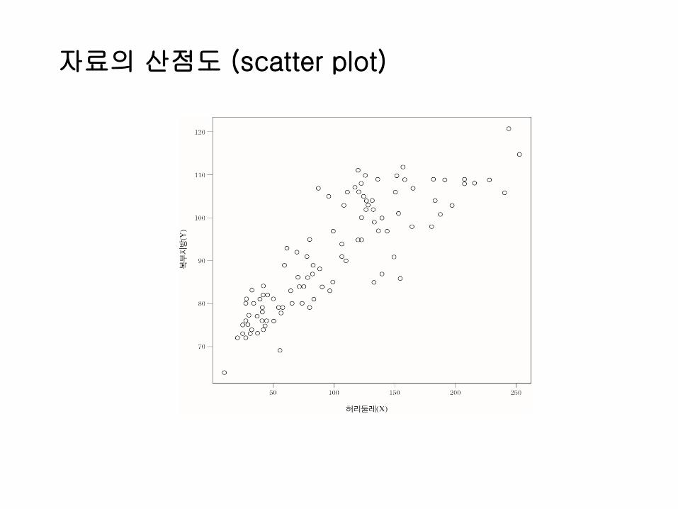
자료의 산점도 (scatter plot)
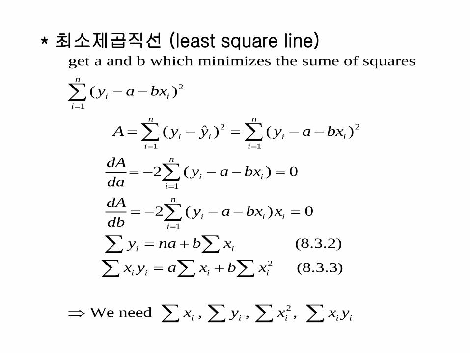
* 최소제곱직선 (least square line)
2
1
2 2
1 1
1
1
2
get a and b which minimizes the sume of squares
( )
ˆ( ) ( )
2 ( ) 0
2 ( ) 0
(8.3.2)
(8.3.3)
We need ,
n
i i
i
n n
i i i i
i i
n
i i
i
n
i i i
i
i i
i i i i
i
y a bx
A y y y a bx
dAy a bx
da
dAy a bx x
db
y na b x
x y a x b x
x y
2, ,i i i ix x y
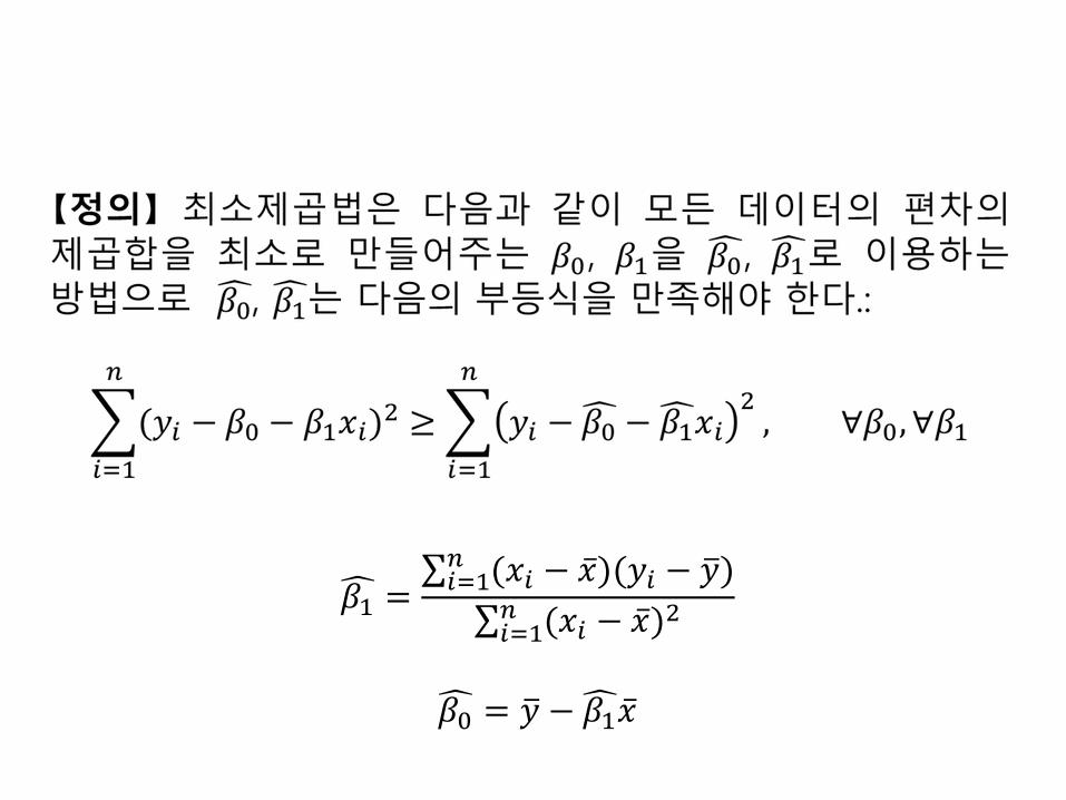
𝛽1 = 𝑖=1𝑛 (𝑥𝑖 − 𝑥)(𝑦𝑖 − 𝑦)
𝑖=1𝑛 (𝑥𝑖 − 𝑥)2
𝛽0 = 𝑦 − 𝛽1 𝑥
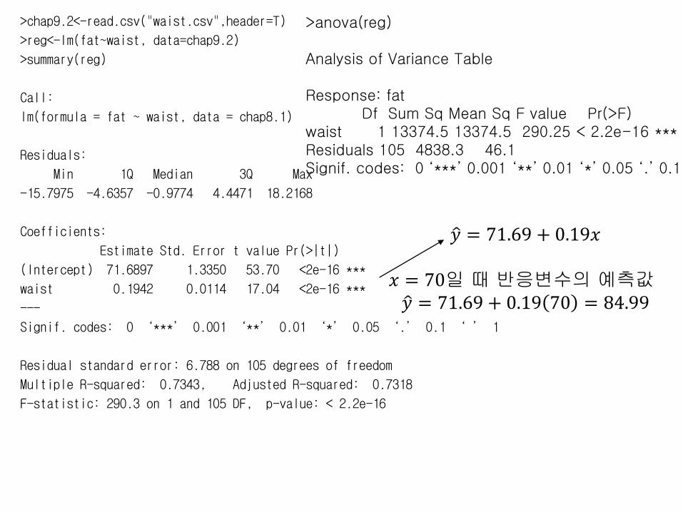
>chap9.2<-read.csv("waist.csv",header=T)
>reg<-lm(fat~waist, data=chap9.2)
>summary(reg)
Call:
lm(formula = fat ~ waist, data = chap8.1)
Residuals:
Min 1Q Median 3Q Max
-15.7975 -4.6357 -0.9774 4.4471 18.2168
Coefficients:
Estimate Std. Error t value Pr(>|t|)
(Intercept) 71.6897 1.3350 53.70 <2e-16 ***
waist 0.1942 0.0114 17.04 <2e-16 ***
---
Signif. codes: 0 ‘***’ 0.001 ‘**’ 0.01 ‘*’ 0.05 ‘.’ 0.1 ‘ ’ 1
Residual standard error: 6.788 on 105 degrees of freedom
Multiple R-squared: 0.7343, Adjusted R-squared: 0.7318
F-statistic: 290.3 on 1 and 105 DF, p-value: < 2.2e-16
>anova(reg)
Analysis of Variance Table
Response: fatDf Sum Sq Mean Sq F value Pr(>F)
waist 1 13374.5 13374.5 290.25 < 2.2e-16 ***Residuals 105 4838.3 46.1 Signif. codes: 0 ‘***’ 0.001 ‘**’ 0.01 ‘*’ 0.05 ‘.’ 0.1 ‘ ’ 1
𝑦 = 71.69 + 0.19𝑥
𝑥 = 70일 때 반응변수의 예측값 𝑦 = 71.69 + 0.19 70 = 84.99
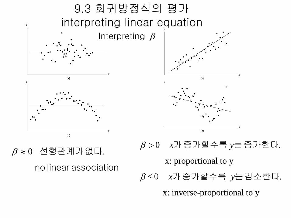
0 선형관계가 없다.
no linear association
0 .
x: proportional to y
.
x: inverse-proportional to y
x y
x y
< 0
가 증가할수록 증가한다
가 증가할수록 는 감소한다
는
Interpreting
9.3 회귀방정식의 평가interpreting linear equation
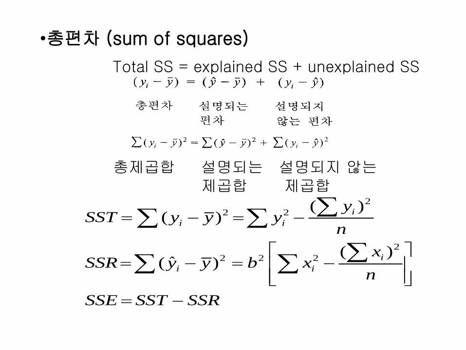
•총편차 (sum of squares)
2
2 2
2
2 2 2
( )( )
( )ˆ( )
i
i i
i
i i
ySST y y y
n
xSSR y y b x
n
SSE SST SSR
Total SS = explained SS + unexplained SS
총제곱합 설명되는 설명되지 않는제곱합 제곱합
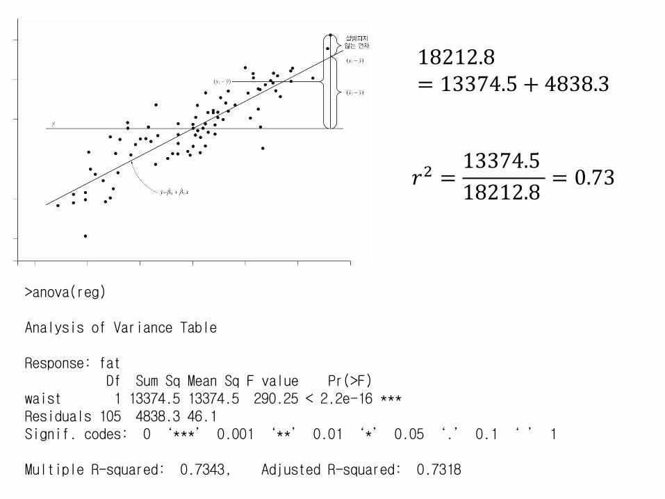
>anova(reg)
Analysis of Variance Table
Response: fatDf Sum Sq Mean Sq F value Pr(>F)
waist 1 13374.5 13374.5 290.25 < 2.2e-16 ***Residuals 105 4838.3 46.1 Signif. codes: 0 ‘***’ 0.001 ‘**’ 0.01 ‘*’ 0.05 ‘.’ 0.1 ‘ ’ 1
Multiple R-squared: 0.7343, Adjusted R-squared: 0.7318
18212.8= 13374.5 + 4838.3
𝑟2 =13374.5
18212.8= 0.73
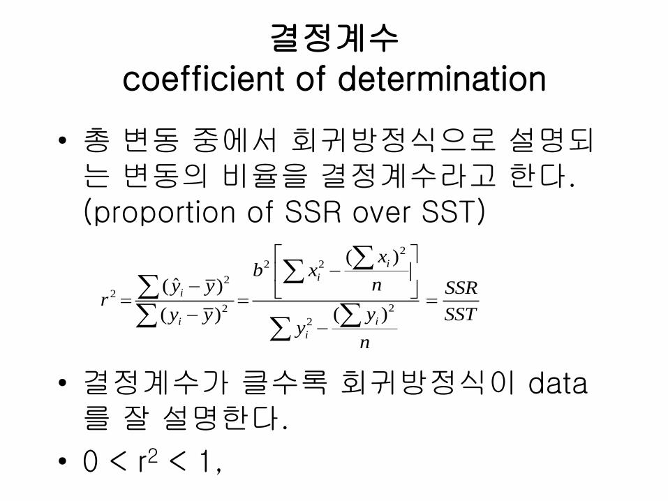
결정계수coefficient of determination
• 총 변동 중에서 회귀방정식으로 설명되는 변동의 비율을 결정계수라고 한다. (proportion of SSR over SST)
• 결정계수가 클수록 회귀방정식이 data를 잘 설명한다.
• 0 < r2 < 1,
2
2 2
2
2
22
2
( )
ˆ( )
( )( )
i
i
i
ii
i
xb x
ny y SSRr
yy y SSTy
n
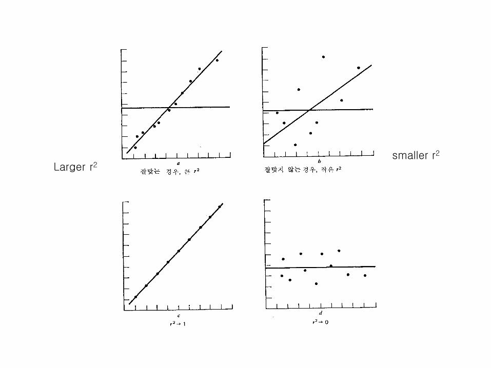
Larger r2smaller r2
FactorModel
ErrorTotal
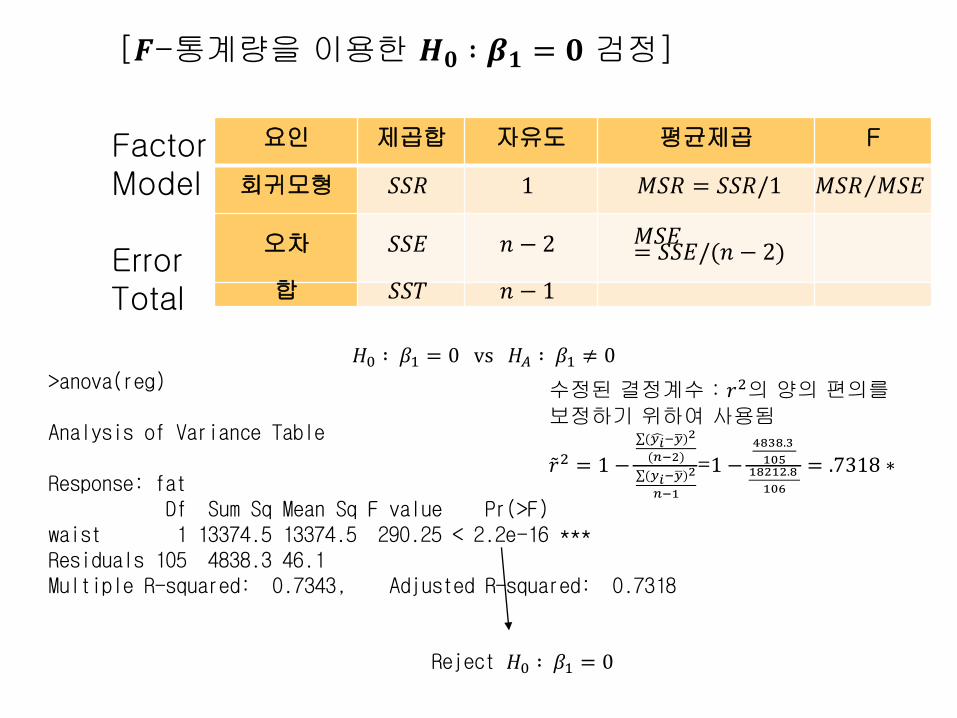
𝐻0 ∶ 𝛽1 = 0 vs 𝐻𝐴 ∶ 𝛽1 ≠ 0>anova(reg)
Analysis of Variance Table
Response: fatDf Sum Sq Mean Sq F value Pr(>F)
waist 1 13374.5 13374.5 290.25 < 2.2e-16 ***Residuals 105 4838.3 46.1Multiple R-squared: 0.7343, Adjusted R-squared: 0.7318
Reject 𝐻0 ∶ 𝛽1 = 0
[𝑭-통계량을 이용한 𝑯𝟎 ∶ 𝜷𝟏 = 𝟎 검정]
요인 제곱합 자유도 평균제곱 F
회귀모형 𝑆𝑆𝑅 1 𝑀𝑆𝑅 = 𝑆𝑆𝑅/1 𝑀𝑆𝑅 𝑀𝑆𝐸
오차 𝑆𝑆𝐸 𝑛 − 2 𝑀𝑆𝐸= 𝑆𝑆𝐸/(𝑛 − 2)
합 𝑆𝑆𝑇 𝑛 − 1
수정된 결정계수 : 𝑟2의 양의 편의를보정하기 위하여 사용됨
𝑟2 = 1 −
( 𝑦𝑖− 𝑦)2
(𝑛−2)
(𝑦𝑖− 𝑦)2
𝑛−1
=1 −4838.3
10518212.8
106
= .7318 ∗
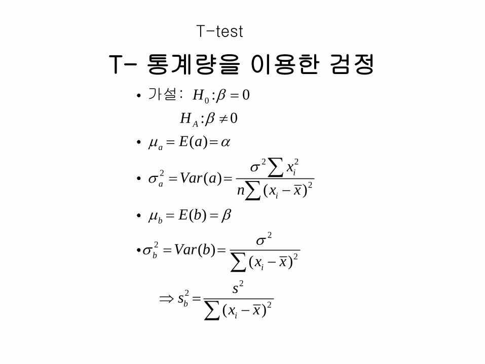
T- 통계량을 이용한 검정
0
2 2
2
2
22
2
22
2
: 0
: 0
( )
( )( )
( )
( )( )
( )
A
a
i
a
i
b
b
i
b
i
H
H
E a
xVar a
n x x
E b
Var bx x
ss
x x
: 가설
T-test
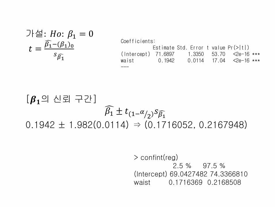
> confint(reg)2.5 % 97.5 %
(Intercept) 69.0427482 74.3366810waist 0.1716369 0.2168508
Coefficients:Estimate Std. Error t value Pr(>|t|)
(Intercept) 71.6897 1.3350 53.70 <2e-16 ***waist 0.1942 0.0114 17.04 <2e-16 ***---
가설: 𝐻𝑜: 𝛽1 = 0
𝑡 = 𝛽1−(𝛽1)0
𝑠 𝛽1
[𝜷𝟏의 신뢰 구간] 𝛽1 ± 𝑡(1− 𝛼 2)
𝑠 𝛽10.1942 ± 1.982(0.0114) ⇒ (0.1716052, 0.2167948)
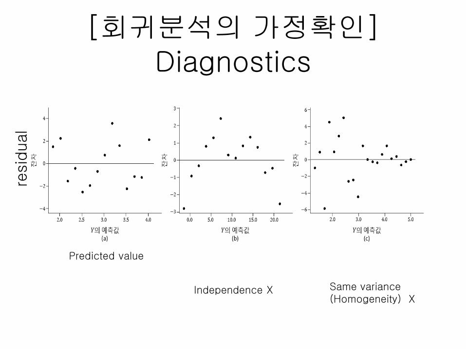
[회귀분석의 가정확인] Diagnostics
Predicted value
resid
ual
Independence X Same variance(Homogeneity) X
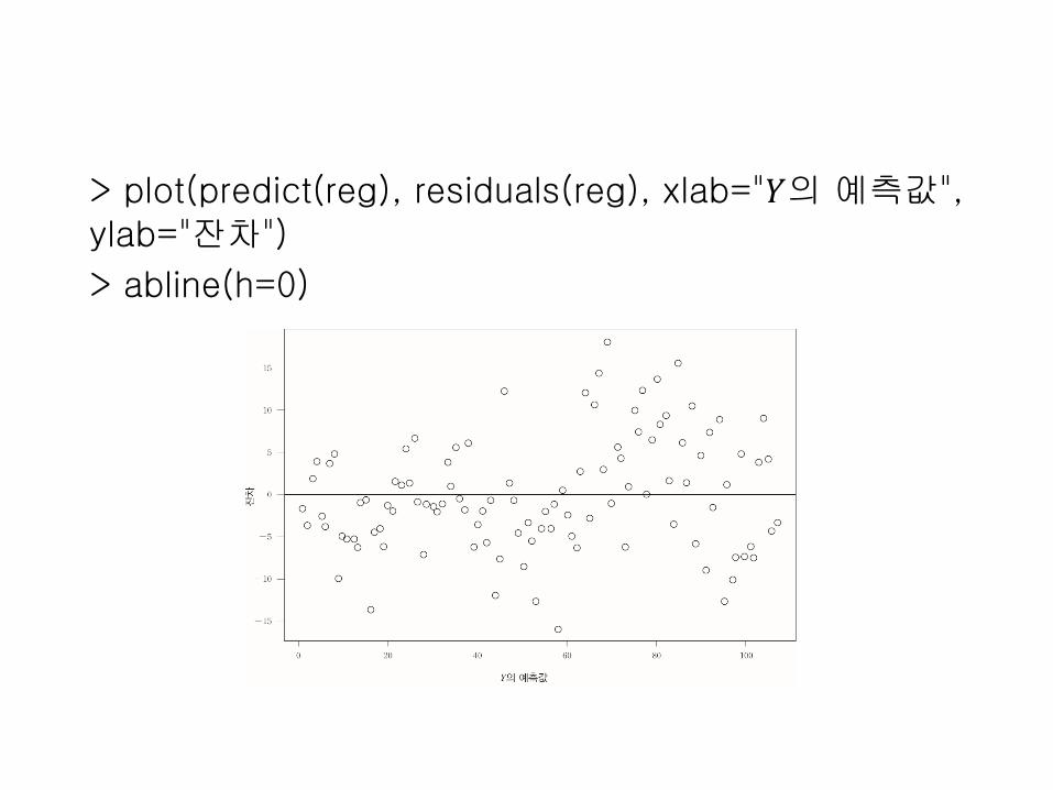
> plot(predict(reg), residuals(reg), xlab="𝑌의 예측값", ylab="잔차")
> abline(h=0)
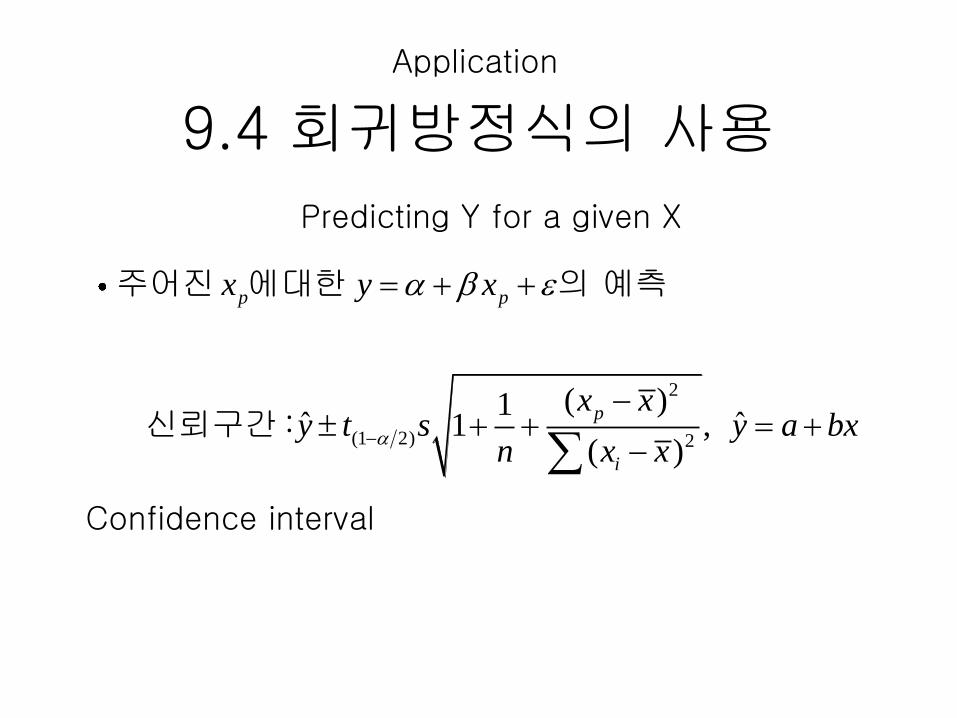
9.4 회귀방정식의 사용
2
(1 2) 2
( )1ˆ ˆ 1 ,
( )
p p
p
i
x y x
x xy t s y a bx
n x x
:
주어진 에 대한 의 예측
신뢰구간
Application
Predicting Y for a given X
Confidence interval
2
(1 2) 2
( )
( )
( )1ˆ ˆ ,
( )
p p
p
p
i
x E y x
x xy t s y a bx
n x x
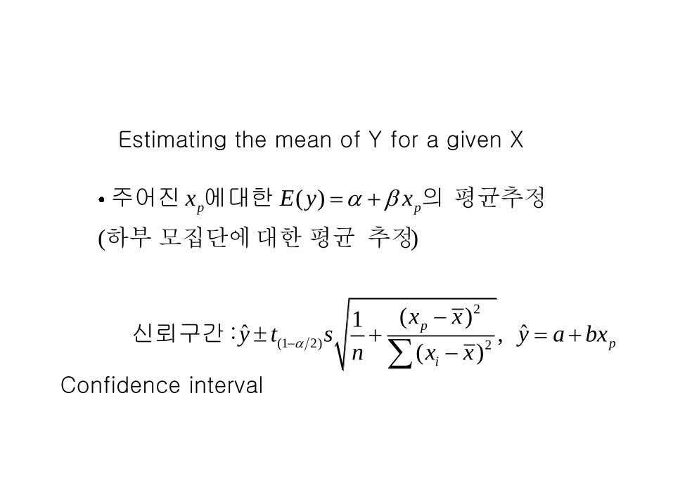
평균추정
하부모집단에대한평균 추정
:
주어진 에 대한 의
신뢰구간
Estimating the mean of Y for a given X
Confidence interval
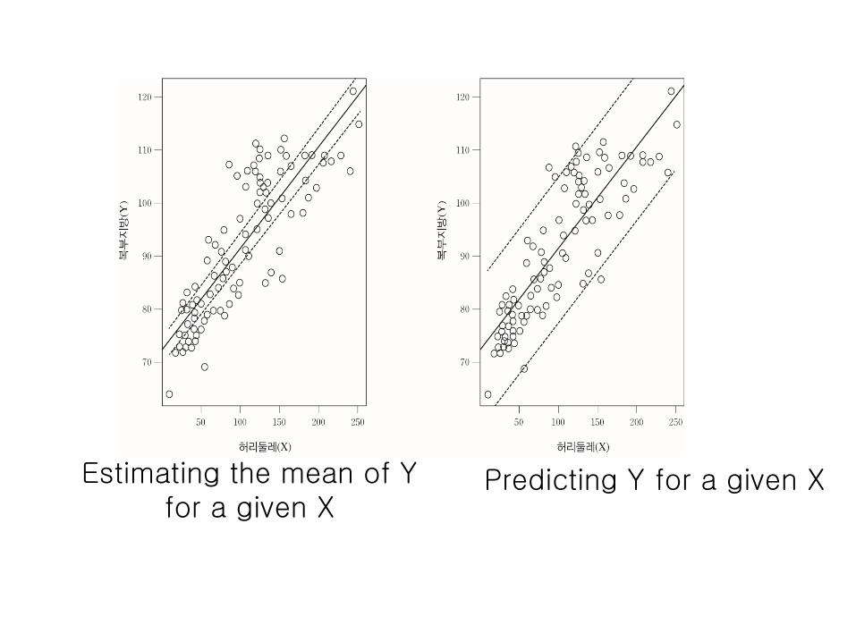
Estimating the mean of Y for a given X
Predicting Y for a given X
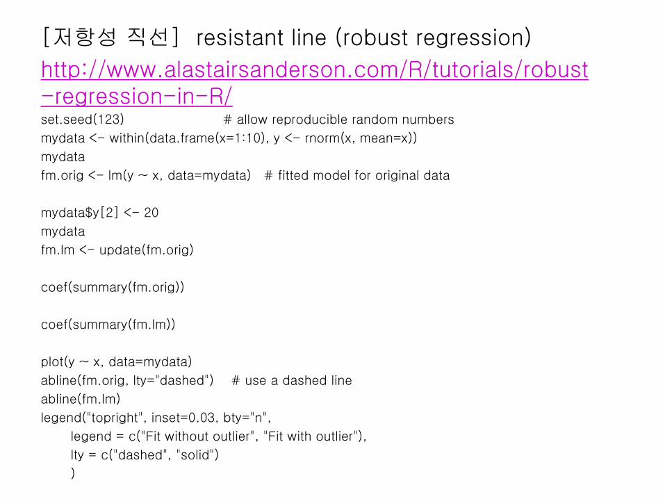
[저항성 직선] resistant line (robust regression)
http://www.alastairsanderson.com/R/tutorials/robust-regression-in-R/set.seed(123) # allow reproducible random numbers
mydata <- within(data.frame(x=1:10), y <- rnorm(x, mean=x))
mydata
fm.orig <- lm(y ~ x, data=mydata) # fitted model for original data
mydata$y[2] <- 20
mydata
fm.lm <- update(fm.orig)
coef(summary(fm.orig))
coef(summary(fm.lm))
plot(y ~ x, data=mydata)
abline(fm.orig, lty="dashed") # use a dashed line
abline(fm.lm)
legend("topright", inset=0.03, bty="n",
legend = c("Fit without outlier", "Fit with outlier"),
lty = c("dashed", "solid")
)
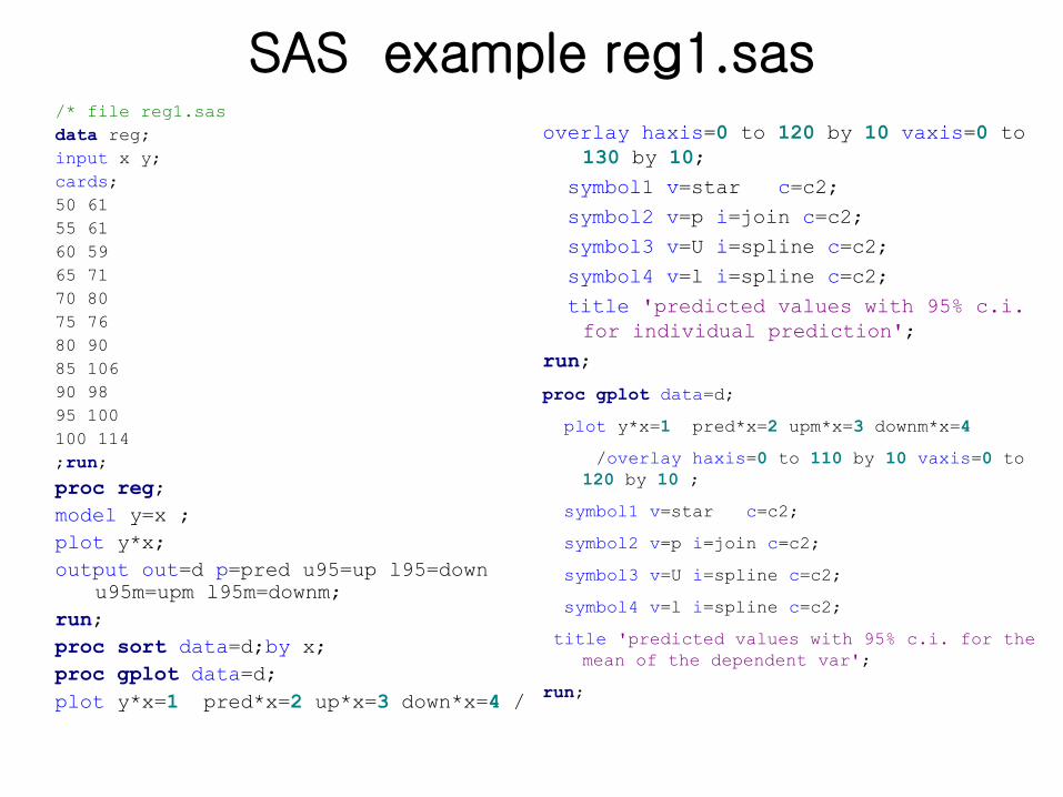
SAS example reg1.sas/* file reg1.sas
data reg;
input x y;
cards;
50 61
55 61
60 59
65 71
70 80
75 76
80 90
85 106
90 98
95 100
100 114
;run;
proc reg;
model y=x ;
plot y*x;
output out=d p=pred u95=up l95=down
u95m=upm l95m=downm;
run;
proc sort data=d;by x;
proc gplot data=d;
plot y*x=1 pred*x=2 up*x=3 down*x=4 /
overlay haxis=0 to 120 by 10 vaxis=0 to
130 by 10;
symbol1 v=star c=c2;
symbol2 v=p i=join c=c2;
symbol3 v=U i=spline c=c2;
symbol4 v=l i=spline c=c2;
title 'predicted values with 95% c.i.
for individual prediction';
run;
proc gplot data=d;
plot y*x=1 pred*x=2 upm*x=3 downm*x=4
/overlay haxis=0 to 110 by 10 vaxis=0 to
120 by 10 ;
symbol1 v=star c=c2;
symbol2 v=p i=join c=c2;
symbol3 v=U i=spline c=c2;
symbol4 v=l i=spline c=c2;
title 'predicted values with 95% c.i. for the
mean of the dependent var';
run;
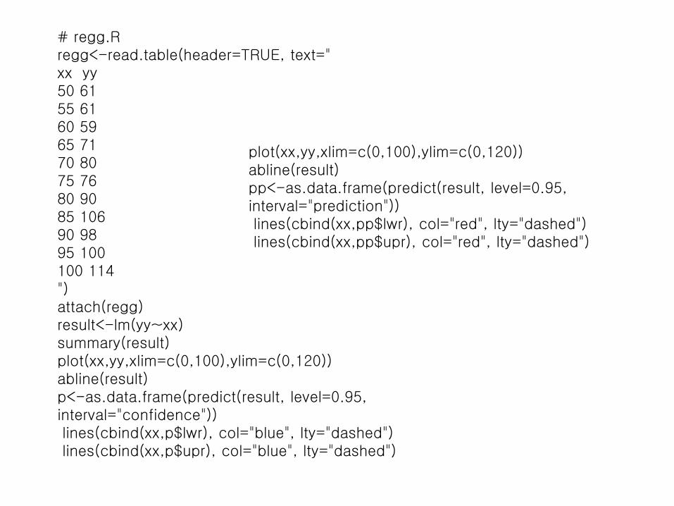
# regg.Rregg<-read.table(header=TRUE, text="xx yy50 6155 6160 5965 7170 8075 7680 9085 10690 9895 100100 114")attach(regg)result<-lm(yy~xx) summary(result)plot(xx,yy,xlim=c(0,100),ylim=c(0,120))abline(result)p<-as.data.frame(predict(result, level=0.95, interval="confidence"))lines(cbind(xx,p$lwr), col="blue", lty="dashed")lines(cbind(xx,p$upr), col="blue", lty="dashed")
plot(xx,yy,xlim=c(0,100),ylim=c(0,120))abline(result)pp<-as.data.frame(predict(result, level=0.95, interval="prediction"))lines(cbind(xx,pp$lwr), col="red", lty="dashed")lines(cbind(xx,pp$upr), col="red", lty="dashed")

9.5 다중회귀분석의 개념
• One Y& k independent variables 1, , kx x
Y
종속변수(Dependent variable)
독립변수
(Independent variable)
반응변수(Response variable)
설명변수(explanatory variable)예측변수(predictor variable)
1, , kx x
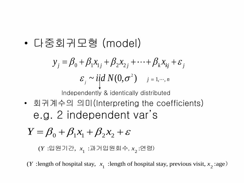
• 다중회귀모형 (model)
• 회귀계수의 의미(Interpreting the coefficients)
e.g. 2 independent var’s
2
0 1 1 2 2
1, ,~ (0, )j
j j j k kj j
j n
y x x x
iid N
Independently & identically distributed
1 2
1 2
0 1 1 2 2
( : , : :
( :length of hospital stay, :length of hospital stay, previous visit, :age
Y x x
Y x x
Y x x
, )
)
입원기간 과거입원회수 연령
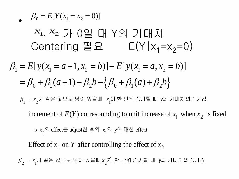
•가 0일 때 Y의 기대치
Centering 필요 E(Y|x1=x2=0)
0 1 2[ ( 0)]E Y x x
1, 2x x
1 2 1
2
1 1 2 1 2
0 1 2 0 1 2
1 2
increment of ( ) corresponding to unit increase of when is fixed
[ ( 1, )] [ ( , )]
( 1) ( )
x x y
x
E Y x x
E y x a x b E y x a x b
a b a b
가 같은 값으로 남아 있을때 이 한 단위 증가할 때 의 기대치 의 증가값
의1
2 1 2
effect adjust y effect
1 2
Effect of on after controlling the effect of
x
x x y
x Y x
가
를 한 후의 의 에 대한
가 같은 값으로 남아 있을때 한 단위 증가할 때 의 기대치 의 증가값
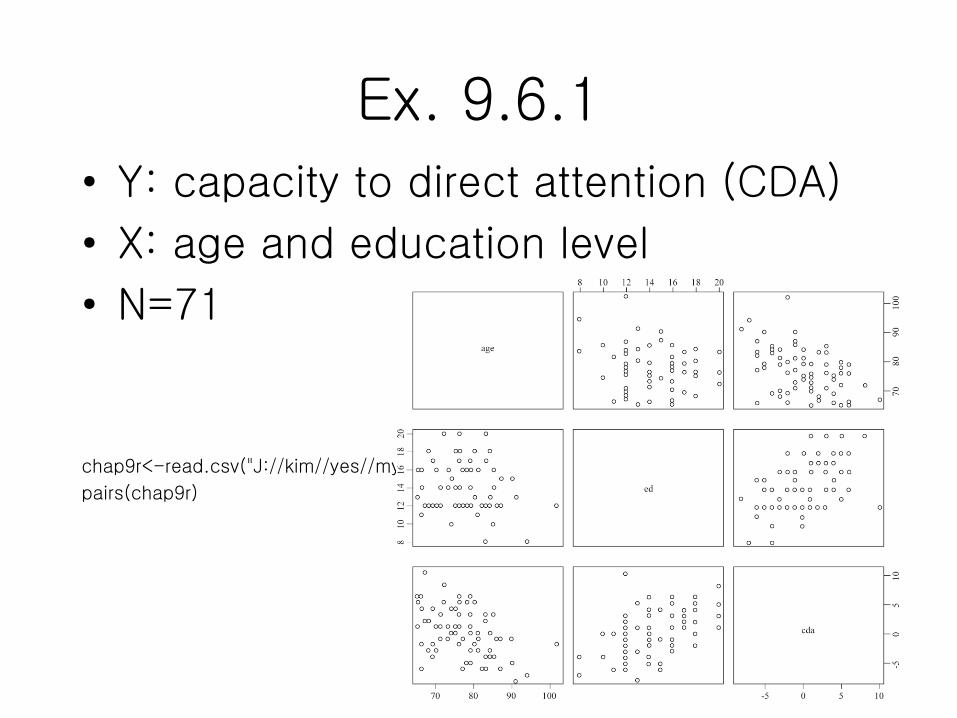
Ex. 9.6.1
• Y: capacity to direct attention (CDA)
• X: age and education level
• N=71
chap9r<-read.csv("J://kim//yes//myweb//int//2017//data//cda.csv",header=T)
pairs(chap9r)
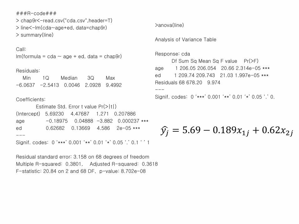
###R-code###
> chap9r<-read.csv("cda.csv",header=T)
> line<-lm(cda~age+ed, data=chap9r)
> summary(line)
Call:
lm(formula = cda ~ age + ed, data = chap9r)
Residuals:
Min 1Q Median 3Q Max
-6.0637 -2.5413 0.0046 2.0928 9.4992
Coefficients:
Estimate Std. Error t value Pr(>|t|)
(Intercept) 5.69230 4.47687 1.271 0.207886
age -0.18975 0.04888 -3.882 0.000237 ***
ed 0.62682 0.13669 4.586 2e-05 ***
---
Signif. codes: 0 ‘***’ 0.001 ‘**’ 0.01 ‘*’ 0.05 ‘.’ 0.1 ‘ ’ 1
Residual standard error: 3.158 on 68 degrees of freedom
Multiple R-squared: 0.3801, Adjusted R-squared: 0.3618
F-statistic: 20.84 on 2 and 68 DF, p-value: 8.702e-08
>anova(line)
Analysis of Variance Table
Response: cda
Df Sum Sq Mean Sq F value Pr(>F)
age 1 206.05 206.054 20.66 2.314e-05 ***
ed 1 209.74 209.743 21.03 1.997e-05 ***
Residuals 68 678.20 9.974
---
Signif. codes: 0 ‘***’ 0.001 ‘**’ 0.01 ‘*’ 0.05 ‘.’ 0.
𝑦𝑗 = 5.69 − 0.189𝑥1𝑗 + 0.62𝑥2𝑗
9.6 다중회귀방정식의 추정(Estimating regression coef.)
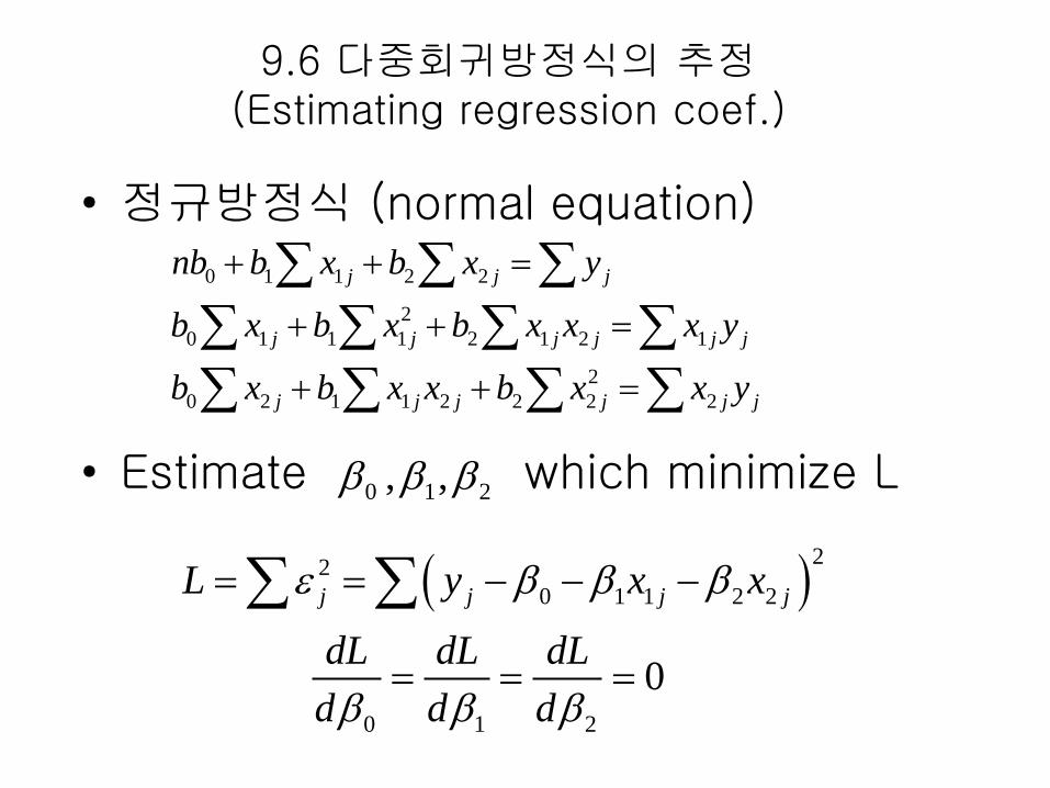
• 정규방정식 (normal equation)
• Estimate which minimize L
0 1 1 2 2
2
0 1 1 1 2 1 2 1
2
0 2 1 1 2 2 2 2
j j j
j j j j j j
j j j j j j
nb b x b x y
b x b x b x x x y
b x b x x b x x y
0 1 2, ,
2
2
0 1 1 2 2
0 1 2
0
j j j jL y x x
dL dL dL
d d d
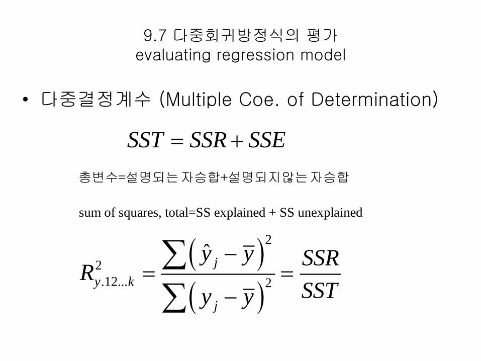
9.7 다중회귀방정식의 평가evaluating regression model
• 다중결정계수 (Multiple Coe. of Determination)
sum of squares, total=SS explained + SS unexplained
2
2
.12... 2
ˆj
y k
j
SST SSR SSE
y y SSRR
SSTy y
총변수=설명되는 자승합+설명되지 않는 자승합
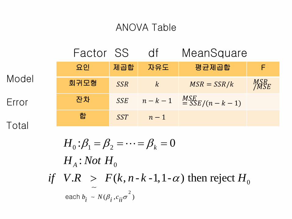
ANOVA Table
2
0 1 2
0
0
( , )
: 0
:
. ( , - -1,1- ) then reject
k
A
b N ci i ii
H
H Not H
if V R F k n k H
each
Model
Error
Total
~
요인 제곱합 자유도 평균제곱합 F
회귀모형 𝑆𝑆𝑅 𝑘 𝑀𝑆𝑅 = 𝑆𝑆𝑅/𝑘 𝑀𝑆𝑅/𝑀𝑆𝐸
잔차 𝑆𝑆𝐸 𝑛 − 𝑘 − 1 𝑀𝑆𝐸= 𝑆𝑆𝐸/(𝑛 − 𝑘 − 1)
합 𝑆𝑆𝑇 𝑛 − 1
Factor SS df MeanSquare
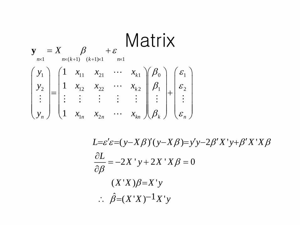
Matrix 1 ( 1) ( 1) 1 1
1 11 21 1 0 1
2 12 22 2 1 2
1 2
1
1
1
( ) ( ) 2 ' '
2 ' 2 ' 0
(
n n k k n
k
k
n n n kn k n
X
y x x x
y x x x
y x x x
L y X y X y y X y X X
LX y X X
X
y
' ) '
ˆ 1( ' ) '
X X y
X X X y
1
1
11 21 1
11 12 1 12 22 2
21 22 2 13 23 3
1 2 1 2
1 2
2
1 1 1 2 1
ˆ ( )
1 1 1 1
1
1
1
k
n k
n k
k k kn n n kn
j j kj
j j j j j kj
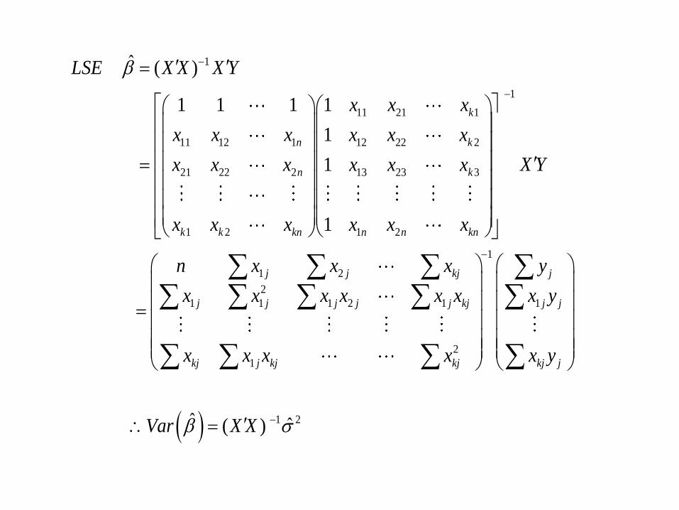
LSE X X X Y
x x x
x x x x x x
X Yx x x x x x
x x x x x x
n x x x
x x x x x x
1
1
2
1
1 2ˆ ˆ( )
j
j j
kj j kj kj kj j
y
x y
x x x x x y
Var X X
1
1 2
2 2
1 1 1 2
2
2 1 2 2
0 0 1 0 2
0 1 1 1 2
0 2 1 2 2
00 01 02
1 2
01 11 12
02 12 22
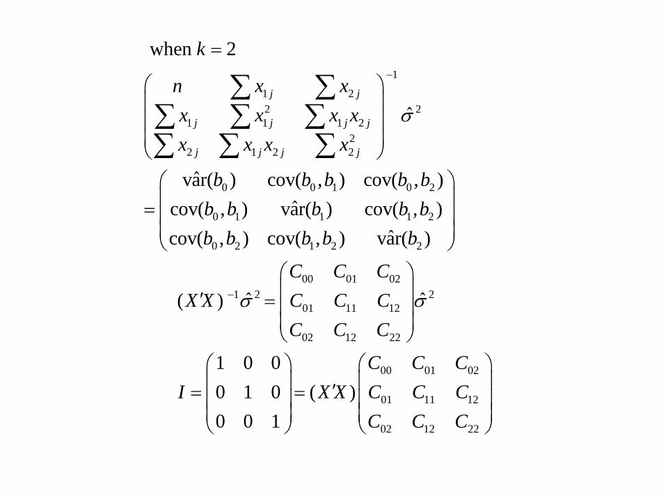
when 2
ˆ
ˆvar( ) cov( , ) cov( , )
ˆcov( , ) var( ) cov( , )
ˆcov( , ) cov( , ) var( )
ˆ( )
j j
j j j j
j j j j
k
n x x
x x x x
x x x x
b b b b b
b b b b b
b b b b b
C C C
X X C C C
C C C
2
00 01 02
01 11 12
02 12 22
ˆ
1 0 0
0 1 0 ( )
0 0 1
C C C
I X X C C C
C C C
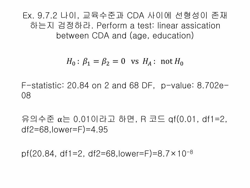
Ex. 9.7.2 나이, 교육수준과 CDA 사이에 선형성이 존재하는지 검정하라. Perform a test: linear assication
between CDA and (age, education)
𝐻0 : 𝛽1 = 𝛽2 = 0 vs 𝐻𝐴 : not 𝐻0
F-statistic: 20.84 on 2 and 68 DF, p-value: 8.702e-08
유의수준 α는 0.01이라고 하면, R 코드 qf(0.01, df1=2, df2=68,lower=F)=4.95
pf(20.84, df1=2, df2=68,lower=F)=8.7×10⁻⁸
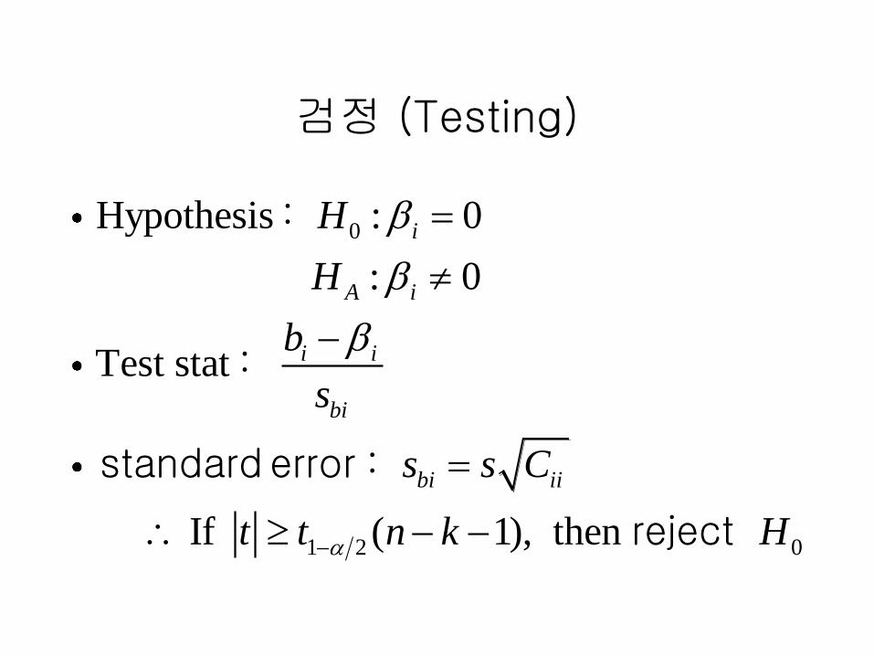
검정 (Testing)
0
1 2 0
Hypothesis : 0
: 0
Test stat
If ( 1), then
i
A i
i i
bi
bi ii
H
H
b
s
s s C
t t n k H
:
:
:
standard error
reject

Ex.9.7.3 나이(연수)는 CDA와 선형성이 있는지 검정하라.Is age significantly associated with CDA?
Coefficients:
Estimate Std. Error t value Pr(>|t|)
(Intercept) 5.69230 4.47687 1.271 0.207886
age -0.18975 0.04888 -3.882 0.000237 ***
ed 0.62682 0.13669 4.586 2e-05 ***
• 𝑡 = 𝛽1−0
𝑠 𝛽1
=−0.189
0.0488= −3.88
• −0.189 ± 1.99 0.0488 = −0.189 ± 0.0971 ⟹(−0.2861,−0.0919)
• 𝑡 = 𝛽2−0
𝑠 𝛽2
=0.62
0.136= 4.5
• 0.62 ± 1.99 0.136 = 0.62 ± 0.270 ⟹ (0.35, 0.89)
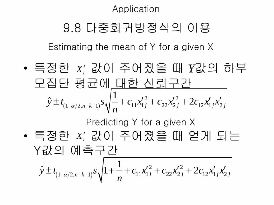
9.8 다중회귀방정식의 이용
• 특정한 값이 주어졌을 때 Y값의 하부
모집단 평균에 대한 신뢰구간
• 특정한 값이 주어졌을 때 얻게 되는Y값의 예측구간
iX
2 2
11 1 22 2 12 1 21 2, 1
1ˆ 2j j j jn ky t s c x c x c x x
n
Application
Predicting Y for a given X
Estimating the mean of Y for a given X
2 2
11 1 22 2 12 1 21 2, 1
1ˆ 1 2j j j jn ky t s c x c x c x x
n
iX

Ex. 9.8.1 12년 동안 교육을 받은 68세 노인들의 CDA 평균에 대한 95% 신뢰구간, 예측구간
95% CI (Confidence Interval) and PI(Prediction Interval) of CDA for (age=68, edu=12)
𝑦 𝑠 𝑦𝑗 95% 신뢰구간 95% 예측구간
0.311 0.677 (−1.04, 1.662) (−6.134, 6.756)
신뢰구간: 12년 동안 교육을 받은 68세 노인들의 CDA 모평균은 95%의 확률로 (−1.04, 1.662)에 포함.부분모집단의 모평균에 대한 구간추정값, interval='confidence'
예측구간: (−6.134, 6.756)관측값의 95% 구간추정값, interval='prediction'
예측구간이 신뢰구간보다 큰 것은 당연
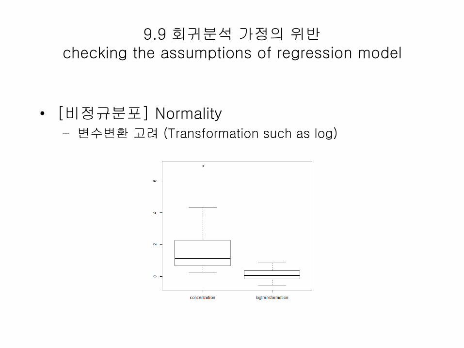
9.9 회귀분석 가정의 위반checking the assumptions of regression model
• [비정규분포] Normality – 변수변환 고려 (Transformation such as log)
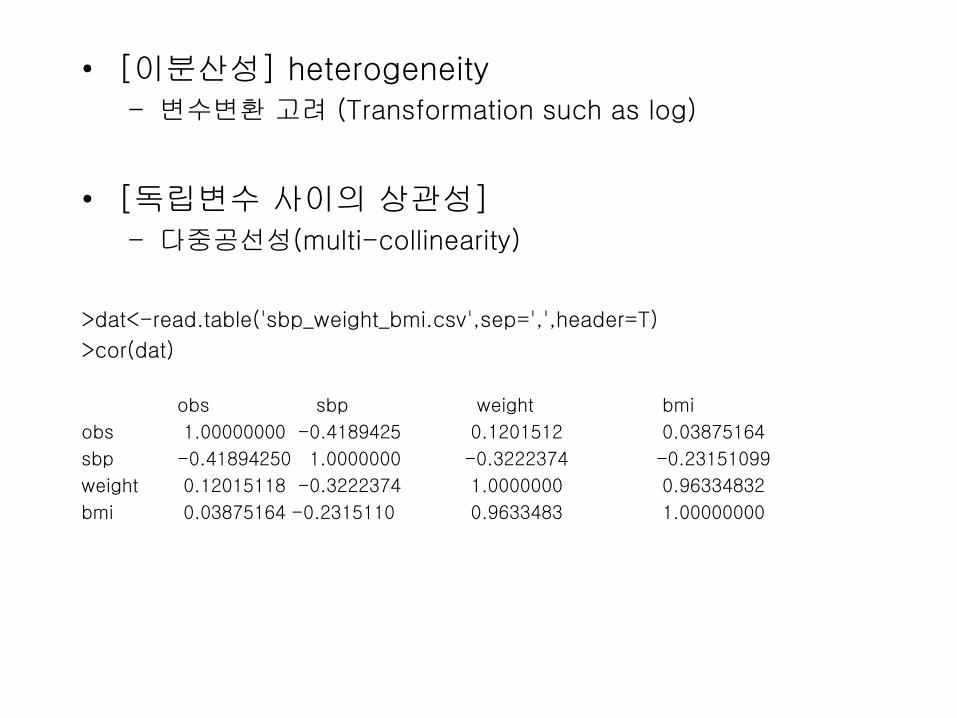
• [이분산성] heterogeneity– 변수변환 고려 (Transformation such as log)
• [독립변수 사이의 상관성] – 다중공선성(multi-collinearity)
>dat<-read.table('sbp_weight_bmi.csv',sep=',',header=T)
>cor(dat)
obs sbp weight bmi
obs 1.00000000 -0.4189425 0.1201512 0.03875164
sbp -0.41894250 1.0000000 -0.3222374 -0.23151099
weight 0.12015118 -0.3222374 1.0000000 0.96334832
bmi 0.03875164 -0.2315110 0.9633483 1.00000000

Assignments
• 1-12