Chapter 9: Consumer Behavior

Source URL: http://web1.boisestate.edu/econ/lreynol/web/Micro.htm Saylor URL: http://www.saylor.org/courses/econ101/ © R. Larry Reynolds, Boise State University (http://web1.boisestate.edu/econ/lreynol/web/) Saylor.org Used by permission. Page 1 of 17

Demand and Consumer Behavior R. Larry Reynolds (2005)

© R. Larry Reynolds 2005 Alternative Microeconomics – Part II, Chapter 9– Demand and Consumer Behavior Page 1

R. Larry Reynolds

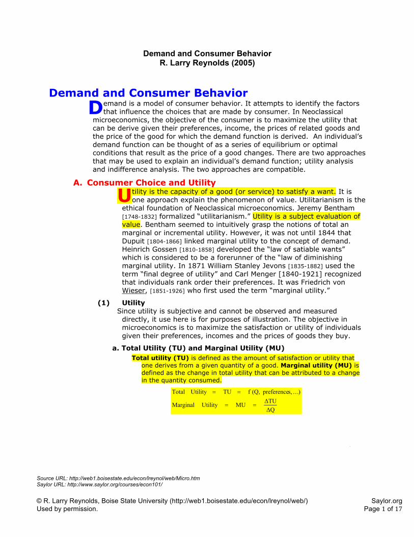
Demand and Consumer Behavior emand is a model of consumer behavior. It attempts to identify the factors that influence the choices that are made by consumer. In Neoclassical

microeconomics, the objective of the consumer is to maximize the utility that can be derive given their preferences, income, the prices of related goods and the price of the good for which the demand function is derived. An individual’s demand function can be thought of as a series of equilibrium or optimal conditions that result as the price of a good changes. There are two approaches that may be used to explain an individual’s demand function; utility analysis and indifference analysis. The two approaches are compatible.

A. Consumer Choice and Utility tility is the capacity of a good (or service) to satisfy a want. It is one approach explain the phenomenon of value. Utilitarianism is the

ethical foundation of Neoclassical microeconomics. Jeremy Bentham [1748-1832] formalized “utilitarianism.” Utility is a subject evaluation of value. Bentham seemed to intuitively grasp the notions of total an marginal or incremental utility. However, it was not until 1844 that Dupuit [1804-1866] linked marginal utility to the concept of demand. Heinrich Gossen [1810-1858] developed the “law of satiable wants” which is considered to be a forerunner of the “law of diminishing marginal utility. In 1871 William Stanley Jevons [1835-1882] used the term “final degree of utility” and Carl Menger [1840-1921] recognized that individuals rank order their preferences. It was Friedrich von Wieser, [1851-1926] who first used the term “marginal utility.”

(1) Utility Since utility is subjective and cannot be observed and measured

directly, it use here is for purposes of illustration. The objective in microeconomics is to maximize the satisfaction or utility of individuals given their preferences, incomes and the prices of goods they buy.

a. Total Utility (TU) and Marginal Utility (MU) Total utility (TU) is defined as the amount of satisfaction or utility that

one derives from a given quantity of a good. Marginal utility (MU) is defined as the change in total utility that can be attributed to a change in the quantity consumed.

ǻQǻTU MU Utility Marginal

) s,preference (Q, f TU UtilityTotal

!

D

U



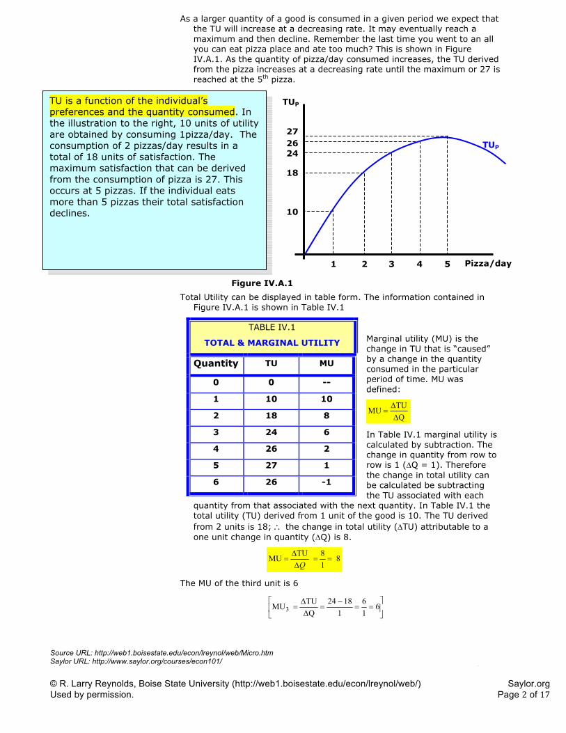
As a larger quantity of a good is consumed in a given period we expect that the TU will increase at a decreasing rate. It may eventually reach a maximum and then decline. Remember the last time you went to an all you can eat pizza place and ate too much? This is shown in Figure IV.A.1. As the quantity of pizza/day consumed increases, the TU derived from the pizza increases at a decreasing rate until the maximum or 27 is reached at the 5th pizza.

Total Utility can be displayed in table form. The information contained in Figure IV.A.1 is shown in Table IV.1

Marginal utility (MU) is the change in TU that is “caused” by a change in the quantity consumed in the particular period of time. MU was defined:

QTUMU''

In Table IV.1 marginal utility is calculated by subtraction. The change in quantity from row to row is 1 ('Q = 1). Therefore the change in total utility can be calculated be subtracting the TU associated with each

quantity from that associated with the next quantity. In Table IV.1 the total utility (TU) derived from 1 unit of the good is 10. The TU derived

from 2 units is 18; ? the change in total utility ('TU) attributable to a one unit change in quantity ('Q) is 8.

818TUMU

''

Q

The MU of the third unit is 6

»¼

º«¬

ª

� 6

16

11824

ǻQǻTUMU 3

TABLE IV.1

TOTAL & MARGINAL UTILITY

Quantity TU MU

0 0 --

1 10 10

2 18 8

3 24 6

4 26 2

5 27 1

6 26 -1

Figure IV.A.1

TUP

Pizza/day

TUP

1 2 3 4 5

10

18

242627

TU is a function of the individual’s preferences and the quantity consumed. In the illustration to the right, 10 units of utilityare obtained by consuming 1pizza/day. The consumption of 2 pizzas/day results in a total of 18 units of satisfaction. The maximum satisfaction that can be derived from the consumption of pizza is 27. This occurs at 5 pizzas. If the individual eats more than 5 pizzas their total satisfaction declines.



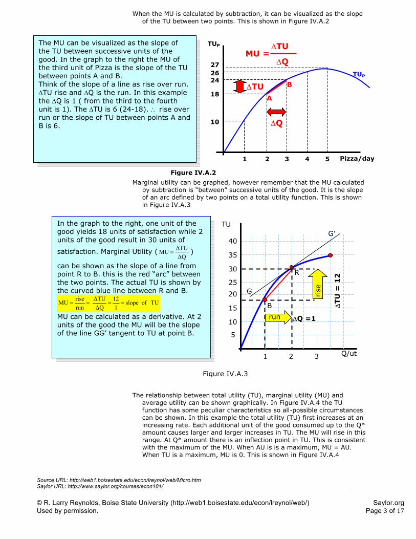
When the MU is calculated by subtraction, it can be visualized as the slope of the TU between two points. This is shown in Figure IV.A.2

Marginal utility can be graphed, however remember that the MU calculated by subtraction is “between” successive units of the good. It is the slope of an arc defined by two points on a total utility function. This is shown in Figure IV.A.3

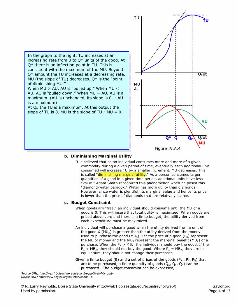
The relationship between total utility (TU), marginal utility (MU) and average utility can be shown graphically. In Figure IV.A.4 the TU function has some peculiar characteristics so all-possible circumstances can be shown. In this example the total utility (TU) first increases at an increasing rate. Each additional unit of the good consumed up to the Q* amount causes larger and larger increases in TU. The MU will rise in this range. At Q* amount there is an inflection point in TU. This is consistent with the maximum of the MU. When AU is is a maximum, MU = AU. When TU is a maximum, MU is 0. This is shown in Figure IV.A.4

Figure IV.A.2

TUP

Pizza/day

TUP

1 2 3 4 5

10

18

242627

The MU can be visualized as the slope of the TU between successive units of the good. In the graph to the right the MU of the third unit of Pizza is the slope of the TU between points A and B. Think of the slope of a line as rise over run. 'TU rise and 'Q is the run. In this example the 'Q is 1 ( from the third to the fourth unit is 1). The 'TU is 6 (24-18). ? rise over run or the slope of TU between points A andB is 6.

'Q

'TU

MU = 'TU

'Q

A

B

Figure IV.A.3

5

10

15

20

25

30

35

40

1 2 3 Q/ut

TU

'Q =1 run rise

'TU

= 1

2

G’

G

In the graph to the right, one unit of the good yields 18 units of satisfaction while 2 units of the good result in 30 units of

satisfaction. Marginal Utility (ǻQǻTUMU )

can be shown as the slope of a line from point R to B. this is the red “arc” between the two points. The actual TU is shown by the curved blue line between R and B.

TUofslope112

ǻQǻTU

runriseMU

MU can be calculated as a derivative. At 2 units of the good the MU will be the slope of the line GG’ tangent to TU at point B.

B

R



TU

Q/ut

Q/ut

MU AU

TU

Q Q* QM

MU

AU

Figure IV.A.4

In the graph to the right, TU increases at an increasing rate from 0 to Q* units of the good. At Q* there is an inflection point in TU. This is consistent with the maximum of the MU. Beyond Q* amount the TU increases at a decreasing rate. MU (the slope of TU) decreases. Q* is the “point of diminishing MU.” When MU > AU, AU is “pulled up.” When MU < AU, AU is “pulled down.” When MU = AU, AU is a maximum. (AU is unchanged, its slope is 0, ?AU is a maximum) At QM the TU is a maximum. At this output the slope of TU is 0. MU is the slope of TU ?MU = 0.

b. Diminishing Marginal Utility It is believed that as an individual consumes more and more of a given

commodity during a given period of time, eventually each additional unit consumed will increase TU by a smaller increment, MU decreases. This is called “diminishing marginal utility.” As a person consumes larger quantities of a good in a given time period, additional units have less “value.” Adam Smith recognized this phenomenon when he posed this “diamond-water paradox.” Water has more utility than diamonds. However, since water is plentiful, its marginal value and hence its price is lower than the price of diamonds that are relatively scarce.

c. Budget Constraint When goods are “free,” an individual should consume until the MU of a

good is 0. This will insure that total utility is maximized. When goods are priced above zero and there is a finite budget, the utility derived from each expenditure must be maximized.

An individual will purchase a good when the utility derived from a unit of the good X (MUX) is greater than the utility derived from the money used to purchase the good (MU$). Let the price of a good (PX) represent the MU of money and the MUX represent the marginal benefit (MBX) of a purchase. When the PX > MBX, the individual should buy the good. If the PX < MBX, they should not buy the good. Where PX = MBX, they are in equilibrium, they should not change their purchases.

Given a finite budget (B) and a set of prices of the goods (PX , PY, PN) that are to be purchased, a finite quantity of goods (QX, QY, QN) can be purchased. The budget constraint can be expressed,



goodNofquantityQ

goodNofpriceP

budgetBWhereQPQPQPB

thN

thN

NNYYXX

��t !

For one good the maximum amount that can be purchased is determined

by the budget and the price of the good. If the budget were 80€ and the

price was 5€, it would be possible to buy 16 units. The amount that can

be purchased is the budget (B) divided by the price of the good (PX).

XX P

BPriceBudgetpurchasedbecanthatQ

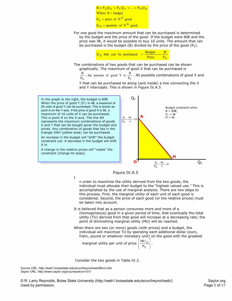
The combinations of two goods that can be purchased can be shown

graphically. The maximum of good X that can be purchased is

YX PBisYgoodofamountthe,

PB

. All possible combinations of good X and

Y that can be purchased lie along (and inside) a line connecting the X

and Y intercepts. This is shown in Figure IV.A.5

I

n order to maximize the utility derived from the two goods, the

individual must allocate their budget to the “highest valued use.” This is

accomplished by the use of marginal analysis. There are two steps to

this process. First, the marginal utility of each unit of each good is

considered. Second, the price of each good (or the relative prices) must

be taken into account.

It is believed that as a person consumes more and more of a

(homogeneous) good in a given period of time, that eventually the total

utility (TU) derived from that good will increase at a decreasing rate; the

point of diminishing marginal utility (MU) will be reached.

When there are two (or more) goods (with prices) and a budget, the

individual will maximize TU by spending each additional dollar (euro,

franc, pound or whatever monetary unit) on the good with the greatest

marginal utility per unit of price »¼

º«¬

ª

X

XPMU

.

Consider the two goods in Table IV.2.

In the graph to the right, the budget is 80€. When the price of good Y (PY) is 4€, a maximum of 20 units of good Y can be purchased. This is shown as point A on the Y-axis. If the price of good X is 5€, a

maximum of 16 units of X can be purchased.

This is point H on the X-axis. The line AH

represents the maximum combinations of goods

X and Y that can be bought given the budget and

prices. Any combination of goods that lies in the

triangle OAH (yellow area) can be purchased.

An increase in the budget will “shift” the budget

constraint out. A decrease in the budget will shift

it in.

A change in the relative prices will “rotate” the

constraint (change its slope).

Budget constraint when

B = 80€, PX = 5€ PY = 4€

QX

QY

20480

YPB

16580

XPB

A

HO

Figure IV.A.5



TABLE IV.2

Maximizing TU of Two Goods Given Prices and Budget (B = $5)

Xebecs (Good X)

PX = $1 - PX1 = $.50

Yawls (Good Y)

PY = $1

QX TUX »¼º

«¬ª

X

X

X

PMU

MU

X1

XP

MU QY TUY MUY YYP

MU

0 0 -- -- 0 0 -- --

1 10 10 20 1 16 16 16

2 18 8 16 2 28 12 12

3 24 6 12 3 36 8 8

4 28 4 4 4 40 4 4

5 30 2 2 5 40 0 0

6 30 0 - 2 6 36 - 4 - 4

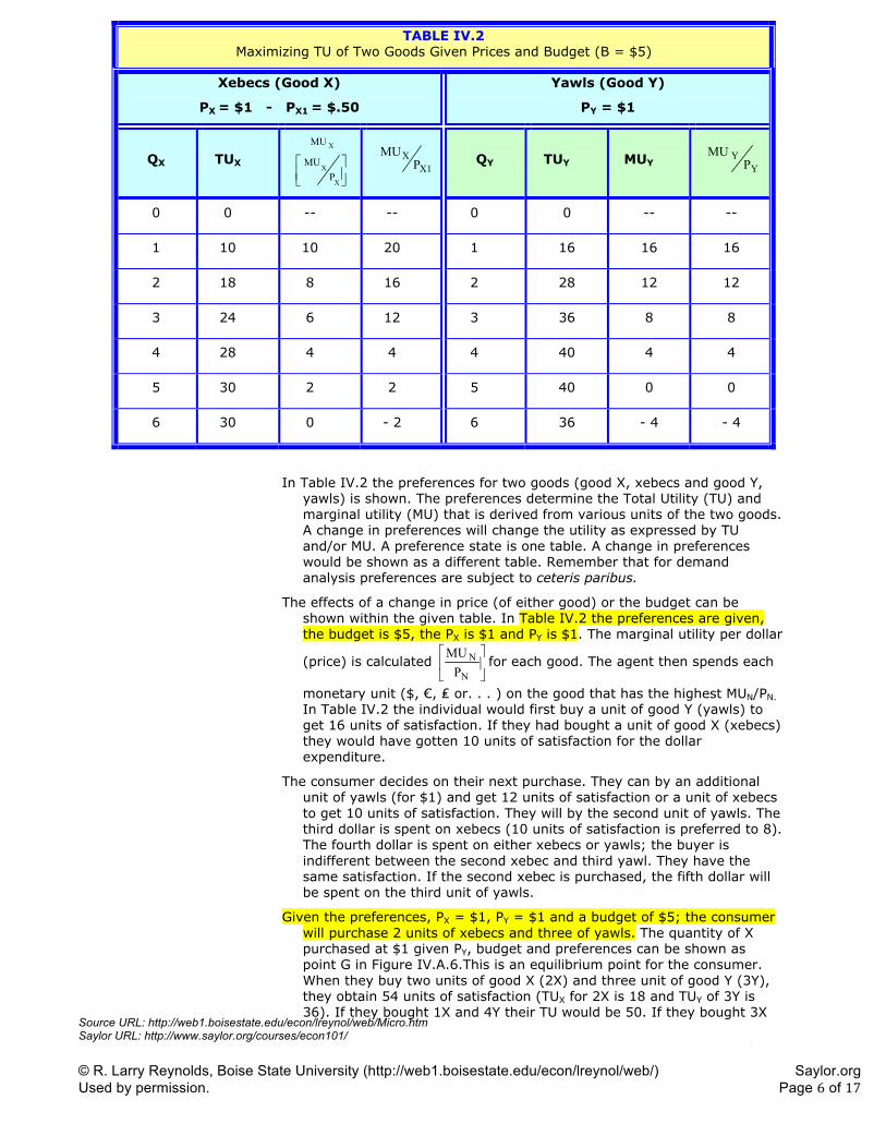
In Table IV.2 the preferences for two goods (good X, xebecs and good Y,

yawls) is shown. The preferences determine the Total Utility (TU) and

marginal utility (MU) that is derived from various units of the two goods.

A change in preferences will change the utility as expressed by TU

and/or MU. A preference state is one table. A change in preferences

would be shown as a different table. Remember that for demand

analysis preferences are subject to ceteris paribus.

The effects of a change in price (of either good) or the budget can be

shown within the given table. In Table IV.2 the preferences are given,

the budget is $5, the PX is $1 and PY is $1. The marginal utility per dollar

(price) is calculated »¼

º«¬

ª

N

NPMU

for each good. The agent then spends each

monetary unit ($, €, ƕ or. . . ) on the good that has the highest MUN/PN.

In Table IV.2 the individual would first buy a unit of good Y (yawls) to

get 16 units of satisfaction. If they had bought a unit of good X (xebecs)

they would have gotten 10 units of satisfaction for the dollar

expenditure.

The consumer decides on their next purchase. They can by an additional

unit of yawls (for $1) and get 12 units of satisfaction or a unit of xebecs

to get 10 units of satisfaction. They will by the second unit of yawls. The

third dollar is spent on xebecs (10 units of satisfaction is preferred to 8).

The fourth dollar is spent on either xebecs or yawls; the buyer is

indifferent between the second xebec and third yawl. They have the

same satisfaction. If the second xebec is purchased, the fifth dollar will

be spent on the third unit of yawls.

Given the preferences, PX = $1, PY = $1 and a budget of $5; the consumer

will purchase 2 units of xebecs and three of yawls. The quantity of X

purchased at $1 given PY, budget and preferences can be shown as

point G in Figure IV.A.6.This is an equilibrium point for the consumer.

When they buy two units of good X (2X) and three unit of good Y (3Y),

they obtain 54 units of satisfaction (TUX for 2X is 18 and TUY of 3Y is

36). If they bought 1X and 4Y their TU would be 50. If they bought 3X



and 2Y their TU is 52. Clearly they cannot increase their utility by altering their purchases.

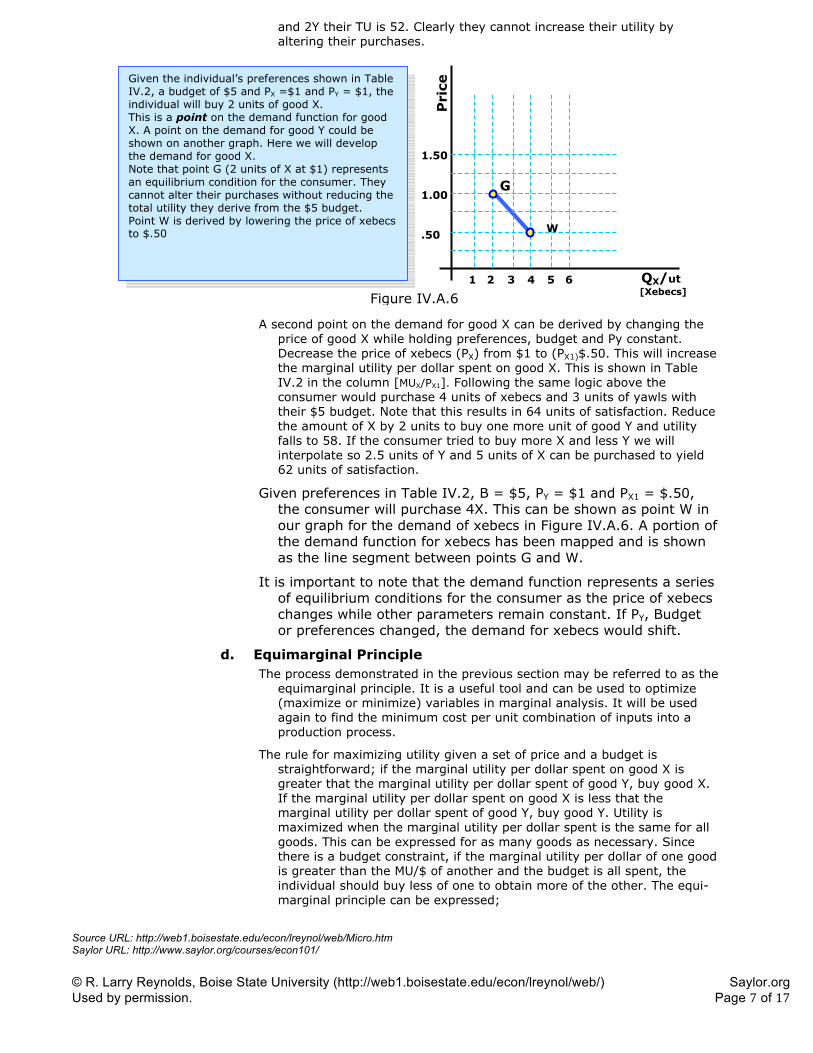
A second point on the demand for good X can be derived by changing the price of good X while holding preferences, budget and Py constant. Decrease the price of xebecs (PX) from $1 to (PX1)$.50. This will increase the marginal utility per dollar spent on good X. This is shown in Table IV.2 in the column [MUX/PX1]. Following the same logic above the consumer would purchase 4 units of xebecs and 3 units of yawls with their $5 budget. Note that this results in 64 units of satisfaction. Reduce the amount of X by 2 units to buy one more unit of good Y and utility falls to 58. If the consumer tried to buy more X and less Y we will interpolate so 2.5 units of Y and 5 units of X can be purchased to yield 62 units of satisfaction.

Given preferences in Table IV.2, B = $5, PY = $1 and PX1 = $.50, the consumer will purchase 4X. This can be shown as point W in our graph for the demand of xebecs in Figure IV.A.6. A portion of the demand function for xebecs has been mapped and is shown as the line segment between points G and W.

It is important to note that the demand function represents a series of equilibrium conditions for the consumer as the price of xebecs changes while other parameters remain constant. If PY, Budget or preferences changed, the demand for xebecs would shift.

d. Equimarginal Principle The process demonstrated in the previous section may be referred to as the

equimarginal principle. It is a useful tool and can be used to optimize (maximize or minimize) variables in marginal analysis. It will be used again to find the minimum cost per unit combination of inputs into a production process.

The rule for maximizing utility given a set of price and a budget is straightforward; if the marginal utility per dollar spent on good X is greater that the marginal utility per dollar spent of good Y, buy good X. If the marginal utility per dollar spent on good X is less that the marginal utility per dollar spent of good Y, buy good Y. Utility is maximized when the marginal utility per dollar spent is the same for all goods. This can be expressed for as many goods as necessary. Since there is a budget constraint, if the marginal utility per dollar of one good is greater than the MU/$ of another and the budget is all spent, the individual should buy less of one to obtain more of the other. The equi-marginal principle can be expressed;

QX/ut

Pri

ce

.50

1.00

1.50

1 2 3 4 5 6

G

[Xebecs]Figure IV.A.6

Given the individual’s preferences shown in Table IV.2, a budget of $5 and PX =$1 and PY = $1, the individual will buy 2 units of good X. This is a point on the demand function for good X. A point on the demand for good Y could be shown on another graph. Here we will develop the demand for good X. Note that point G (2 units of X at $1) represents an equilibrium condition for the consumer. They cannot alter their purchases without reducing the total utility they derive from the $5 budget. Point W is derived by lowering the price of xebecs to $.50 W



PnMUn ==

Py

MUy = Px

MUx " ,

subject to the constraint, B >� PxQx + PyQy + ... + PnQn Where Pni = price of ith good, Qni = quantity of ith good and B = budget

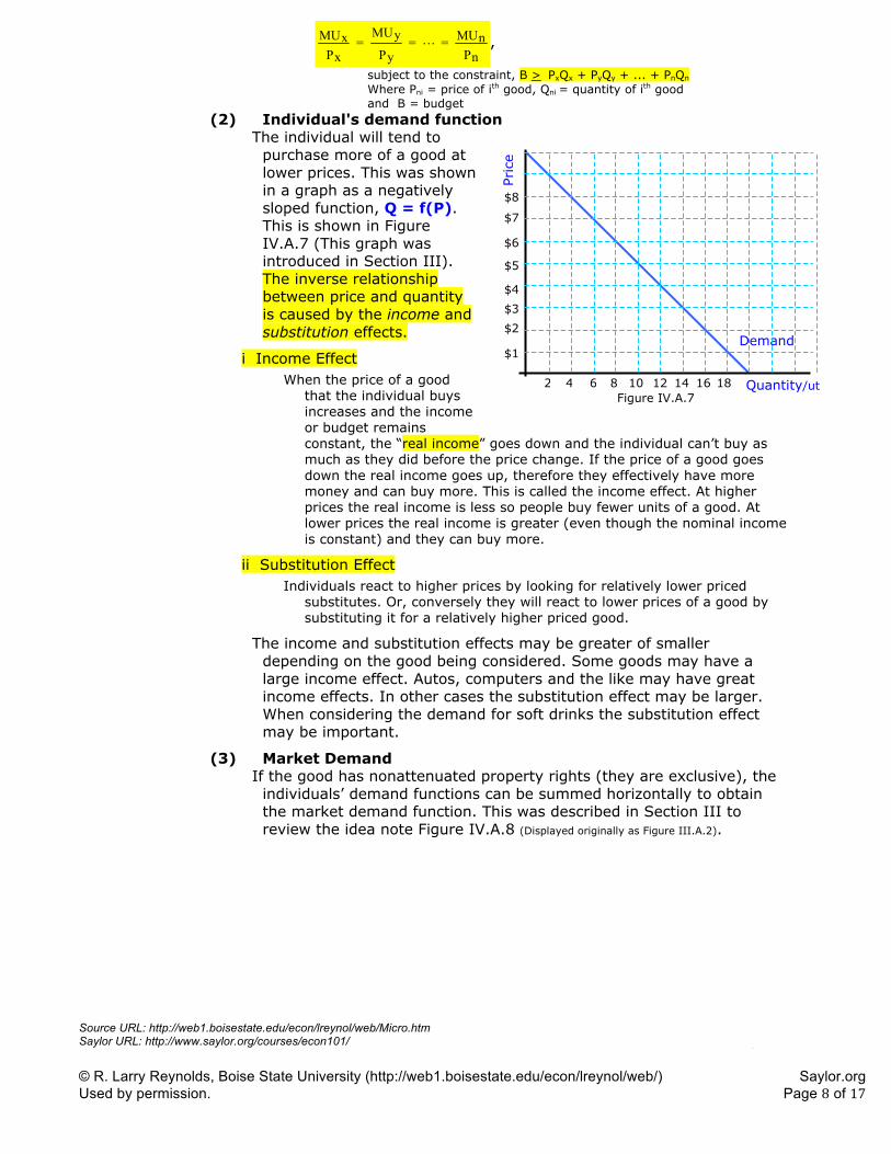
(2) Individual's demand function The individual will tend to

purchase more of a good at lower prices. This was shown in a graph as a negatively sloped function, Q = f(P). This is shown in Figure IV.A.7 (This graph was introduced in Section III). The inverse relationship between price and quantity is caused by the income and substitution effects.

i Income Effect When the price of a good

that the individual buys increases and the income or budget remains constant, the “real income” goes down and the individual can’t buy as much as they did before the price change. If the price of a good goes down the real income goes up, therefore they effectively have more money and can buy more. This is called the income effect. At higher prices the real income is less so people buy fewer units of a good. At lower prices the real income is greater (even though the nominal income is constant) and they can buy more.

ii Substitution Effect Individuals react to higher prices by looking for relatively lower priced

substitutes. Or, conversely they will react to lower prices of a good by substituting it for a relatively higher priced good.

The income and substitution effects may be greater of smaller depending on the good being considered. Some goods may have a large income effect. Autos, computers and the like may have great income effects. In other cases the substitution effect may be larger. When considering the demand for soft drinks the substitution effect may be important.

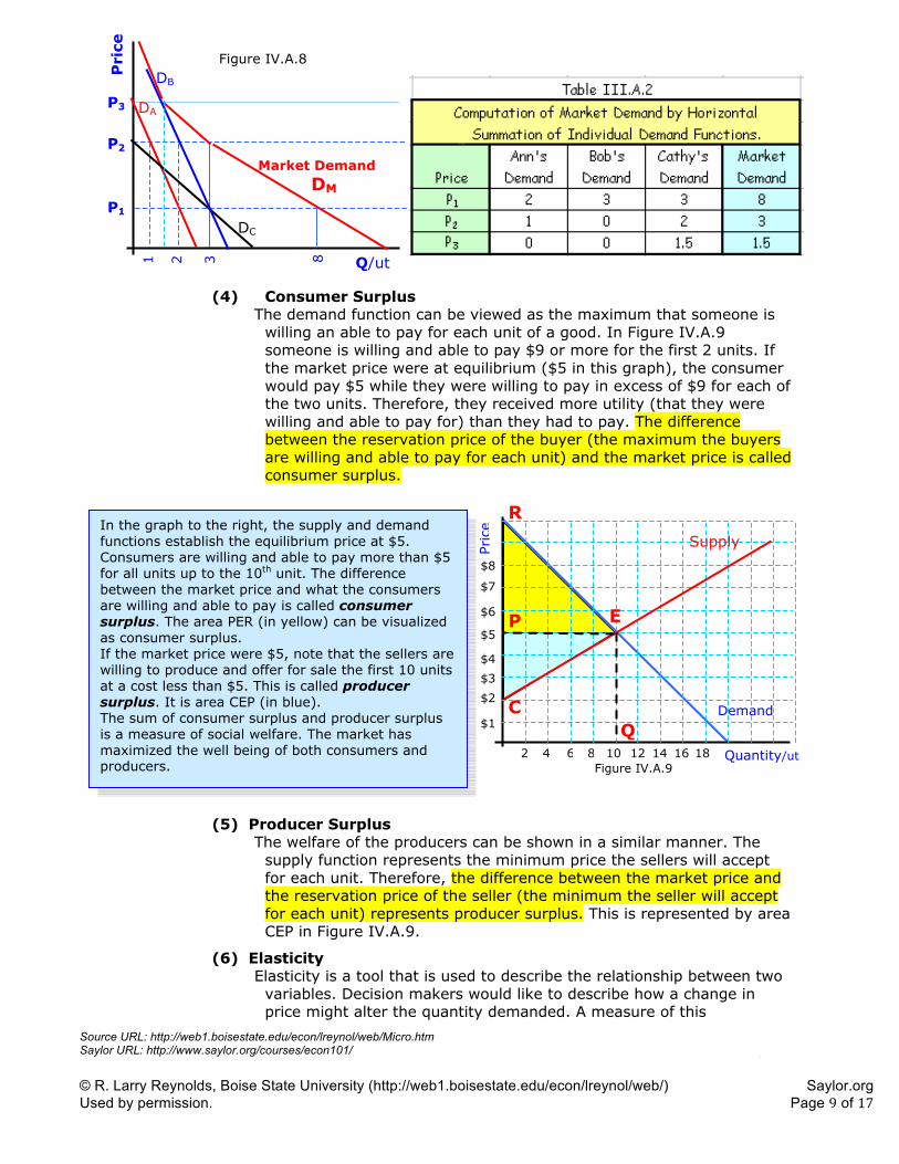
(3) Market Demand If the good has nonattenuated property rights (they are exclusive), the

individuals’ demand functions can be summed horizontally to obtain the market demand function. This was described in Section III to review the idea note Figure IV.A.8 (Displayed originally as Figure III.A.2).

Figure IV.A.7

Demand

Quantity/ut

Pric

e

$1

$2

$3

$4

$5

$6

$7

$8

2 4 6 8 1210 14 16 18



(4) Consumer Surplus The demand function can be viewed as the maximum that someone is

willing an able to pay for each unit of a good. In Figure IV.A.9 someone is willing and able to pay $9 or more for the first 2 units. If the market price were at equilibrium ($5 in this graph), the consumer would pay $5 while they were willing to pay in excess of $9 for each of the two units. Therefore, they received more utility (that they were willing and able to pay for) than they had to pay. The difference between the reservation price of the buyer (the maximum the buyers are willing and able to pay for each unit) and the market price is called consumer surplus.

(5) Producer Surplus The welfare of the producers can be shown in a similar manner. The

supply function represents the minimum price the sellers will accept for each unit. Therefore, the difference between the market price and the reservation price of the seller (the minimum the seller will accept for each unit) represents producer surplus. This is represented by area CEP in Figure IV.A.9.

(6) Elasticity Elasticity is a tool that is used to describe the relationship between two

variables. Decision makers would like to describe how a change in price might alter the quantity demanded. A measure of this

Market Demand DM

Q/ut

Pri

ce

1

2

3

DA

DB

DC

8

P1

P2

P3

Figure IV.A.8

Figure IV.A.9

Demand

Quantity/ut

Pric

e

$1

$2

$3

$4

$5

$6

$7

$8

2 4 6 8 1210 14 16 18

Supply

E

R

P

C Q

In the graph to the right, the supply and demand functions establish the equilibrium price at $5. Consumers are willing and able to pay more than $5 for all units up to the 10th unit. The difference between the market price and what the consumers are willing and able to pay is called consumer surplus. The area PER (in yellow) can be visualized as consumer surplus. If the market price were $5, note that the sellers are willing to produce and offer for sale the first 10 units at a cost less than $5. This is called producer surplus. It is area CEP (in blue). The sum of consumer surplus and producer surplus is a measure of social welfare. The market has maximized the well being of both consumers and producers.



relationship is called the “own” price elasticity of demand. It is also useful to describe how a change in buyers’ income shifts the demand function for a good; this measure is called income elasticity. When the price of a related good (substitute or compliment) changes, the demand for a good will shift. Cross elasticity is a measure of the responsiveness of buyers of a good to changes in the prices of related goods.

Elasticity is defined as

variable tindependen the of change percentagevariable dependent the of change percentage

E ,

This is the percentage change in the dependent variable caused by a percentage change in the independent variable.

(a) "Own" price elasticity of demand [EP or Hp ] i. Definition of EP

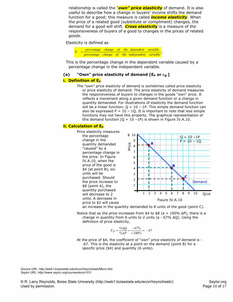
The “own” price elasticity of demand is sometimes called price elasticity or price elasticity of demand. The price elasticity of demand measures the responsiveness of buyers to changes in the goods “own” price. It reflects a movement along a given demand function or a change in quantity demanded. For illustrations of elasticity the demand function will be a linear function; Q = 10 – 1P. This simple demand function can also be expressed P = 10 – 1Q. It is important to note that less simple functions may not have this property. The graphical representation of this demand function (Q = 10 –1P) is shown in Figure IV.A.10.

ii. Calculation of EP Price elasticity measures

the percentage change in the quantity demanded “caused” by a percentage change in the price. In Figure IV.A.10, when the price of the good is $4 (at point B), six units will be purchased. Should the price increase to $8 (point A), the quantity purchased will decrease to 2 units. A decrease in price to $2 will cause an increase in the quantity demanded to 8 units of the good (point C).

Notice that as the price increases from $4 to $8 (a + 100% ƩP), there is a change in quantity from 6 units to 2 units (a - 67% ƩQ). Using the definition of price elasticity,

67.%100%67

%%

� ��

''

PQ

EP

At the price of $4, the coefficient of “own” price elasticity of demand is -.67. This is the elasticity at a point on the demand (point B) for a specific price ($4) and quantity (6 units).

Figure IV.A.10

Pric

e

Q/ut

$

1 2 3 4 5 6 7 8 9 10

1

2

3

4

5

6

7

8

9

10Q = 10 –1P P = 10 – 1Q

Demand

A

B

C



A formula for calculating point price elasticity is:

1

1

1

1QP

xPQ

PP

QQ

=

PP - P

QQ - Q

= E

1

21

1

21

P ''

'

'

Calculating the EP for a price change from $4 to $2 in Figure IV.A.10 , a move from point B to point C:

67.641

64

222,22$,84$,6

1

1

22

11

� � ��

''

� '� '

QP

PQ

E

PQPunitsQPunitsQ

P

Note that the EP is the same whether the price is increased from $4 to $8 or decreased from $4 to $2. The magnitude of the change does not affect the EP either. The coefficient of “own” price elasticity is unique to each point on the demand function. To calculate EP as the price falls from $8 to $4 (a move from point A to point B in Figure IV.A.10):

2141

28

444,44$,68$,2

1

1

22

11

��

''

� '� '

QP

PQ

E

PQPunitsQPunitsQ

P

EP at $8 is –2, at $4 it is -.67. The coefficient is different at every point on the demand function even though the slope of the demand function is the same at every point. EP is determined by the slope of the demand

»¼º

«¬ª

''

PQ and the location on the demand »¼

º«¬ª

11

QP .

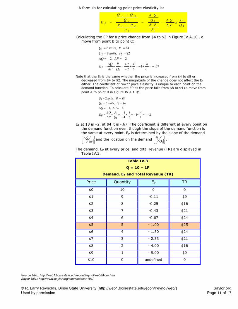
The demand, EP at every price, and total revenue (TR) are displayed in Table IV.3.

Table IV.3

Q = 10 – 1P

Demand, EP and Total Revenue (TR)

Price Quantity EP TR

$0 10 0 0

$1 9 -0.11 $9

$2 8 -0.25 $16

$3 7 -0.43 $21

$4 6 -0.67 $24

$5 5 - 1.00 $25

$6 4 - 1.50 $24

$7 3 - 2.33 $21

$8 2 - 4.00 $16

$9 1 - 9.00 $9

$10 0 undefined 0



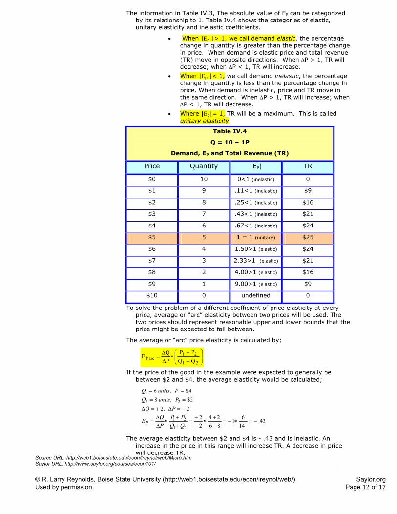
The information in Table IV.3, The absolute value of EP can be categorized by its relationship to 1. Table IV.4 shows the categories of elastic, unitary elasticity and inelastic coefficients.

x� When |(p |> 1, we call demand elastic, the percentage change in quantity is greater than the percentage change in price. When demand is elastic price and total revenue (TR) move in opposite directions. When 'P > 1, TR will decrease; when 'P < 1, TR will increase.

x� When |(p |< 1, we call demand inelastic, the percentage change in quantity is less than the percentage change in price. When demand is inelastic, price and TR move in the same direction. When 'P > 1, TR will increase; when 'P < 1, TR will decrease.

x� Where |(p|= 1, TR will be a maximum. This is called unitary elasticity

Table IV.4

Q = 10 – 1P

Demand, EP and Total Revenue (TR)

Price Quantity |EP| TR

$0 10 0<1 (inelastic) 0

$1 9 .11<1 (inelastic) $9

$2 8 .25<1 (inelastic) $16

$3 7 .43<1 (inelastic) $21

$4 6 .67<1 (inelastic) $24

$5 5 1 = 1 (unitary) $25

$6 4 1.50>1 (elastic) $24

$7 3 2.33>1 (elastic) $21

$8 2 4.00>1 (elastic) $16

$9 1 9.00>1 (elastic) $9

$10 0 undefined 0

To solve the problem of a different coefficient of price elasticity at every price, average or “arc” elasticity between two prices will be used. The two prices should represent reasonable upper and lower bounds that the price might be expected to fall between.

The average or “arc” price elasticity is calculated by;

¸̧¹

·¨̈©

§��

21

21arcP QQ

PPǻPǻQE

If the price of the good in the example were expected to generally be between $2 and $4, the average elasticity would be calculated;

43.1461

8624

22

2,22$,84$,6

21

21

22

11

� � ��

��

��

''

� '� '

QQPP

PQE

PQPunitsQPunitsQ

P

The average elasticity between $2 and $4 is - .43 and is inelastic. An increase in the price in this range will increase TR. A decrease in price will decrease TR.



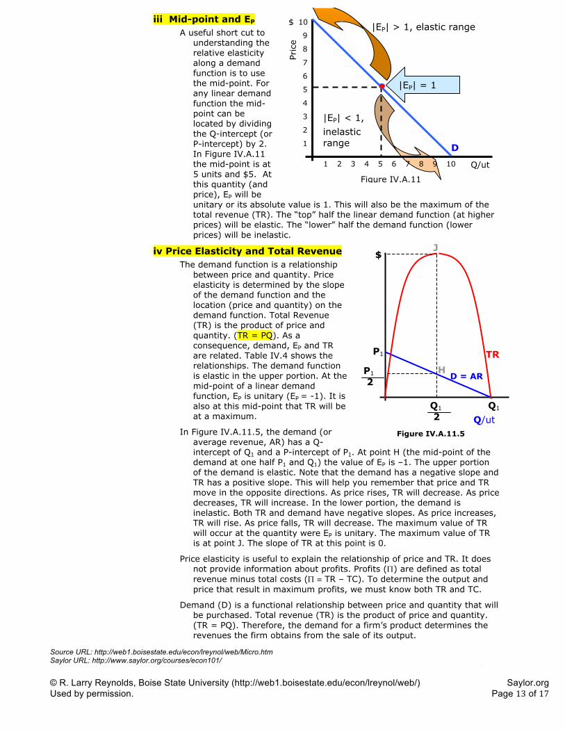
iii Mid-point and EP A useful short cut to

understanding the relative elasticity along a demand function is to use the mid-point. For any linear demand function the mid-point can be located by dividing the Q-intercept (or P-intercept) by 2. In Figure IV.A.11 the mid-point is at 5 units and $5. At this quantity (and price), EP will be unitary or its absolute value is 1. This will also be the maximum of the total revenue (TR). The “top” half the linear demand function (at higher prices) will be elastic. The “lower” half the demand function (lower prices) will be inelastic.

iv Price Elasticity and Total Revenue The demand function is a relationship

between price and quantity. Price elasticity is determined by the slope of the demand function and the location (price and quantity) on the demand function. Total Revenue (TR) is the product of price and quantity. (TR = PQ). As a consequence, demand, EP and TR are related. Table IV.4 shows the relationships. The demand function is elastic in the upper portion. At the mid-point of a linear demand function, EP is unitary (EP = -1). It is also at this mid-point that TR will be at a maximum.

In Figure IV.A.11.5, the demand (or average revenue, AR) has a Q-intercept of Q1 and a P-intercept of P1. At point H (the mid-point of the demand at one half P1 and Q1) the value of EP is –1. The upper portion of the demand is elastic. Note that the demand has a negative slope and TR has a positive slope. This will help you remember that price and TR move in the opposite directions. As price rises, TR will decrease. As price decreases, TR will increase. In the lower portion, the demand is inelastic. Both TR and demand have negative slopes. As price increases, TR will rise. As price falls, TR will decrease. The maximum value of TR will occur at the quantity were EP is unitary. The maximum value of TR is at point J. The slope of TR at this point is 0.

Price elasticity is useful to explain the relationship of price and TR. It does not provide information about profits. Profits (3) are defined as total revenue minus total costs (3 { TR – TC). To determine the output and price that result in maximum profits, we must know both TR and TC.

Demand (D) is a functional relationship between price and quantity that will be purchased. Total revenue (TR) is the product of price and quantity. (TR = PQ). Therefore, the demand for a firm’s product determines the revenues the firm obtains from the sale of its output.

|EP| < 1,

inelastic range

|EP| > 1, elastic range

|EP| = 1

1 2 3 4 5 6 7 8 9 10

1

2

3

4

5

6

7

8

9

10

Figure IV.A.11

Pric

e

Q/ut

$

D

Q/ut

$

H

Q1 Q1

2

P1

P1

2 D = AR

TR

J

Figure IV.A.11.5



Q220Q

2Q20QQ

TRAR2

� �

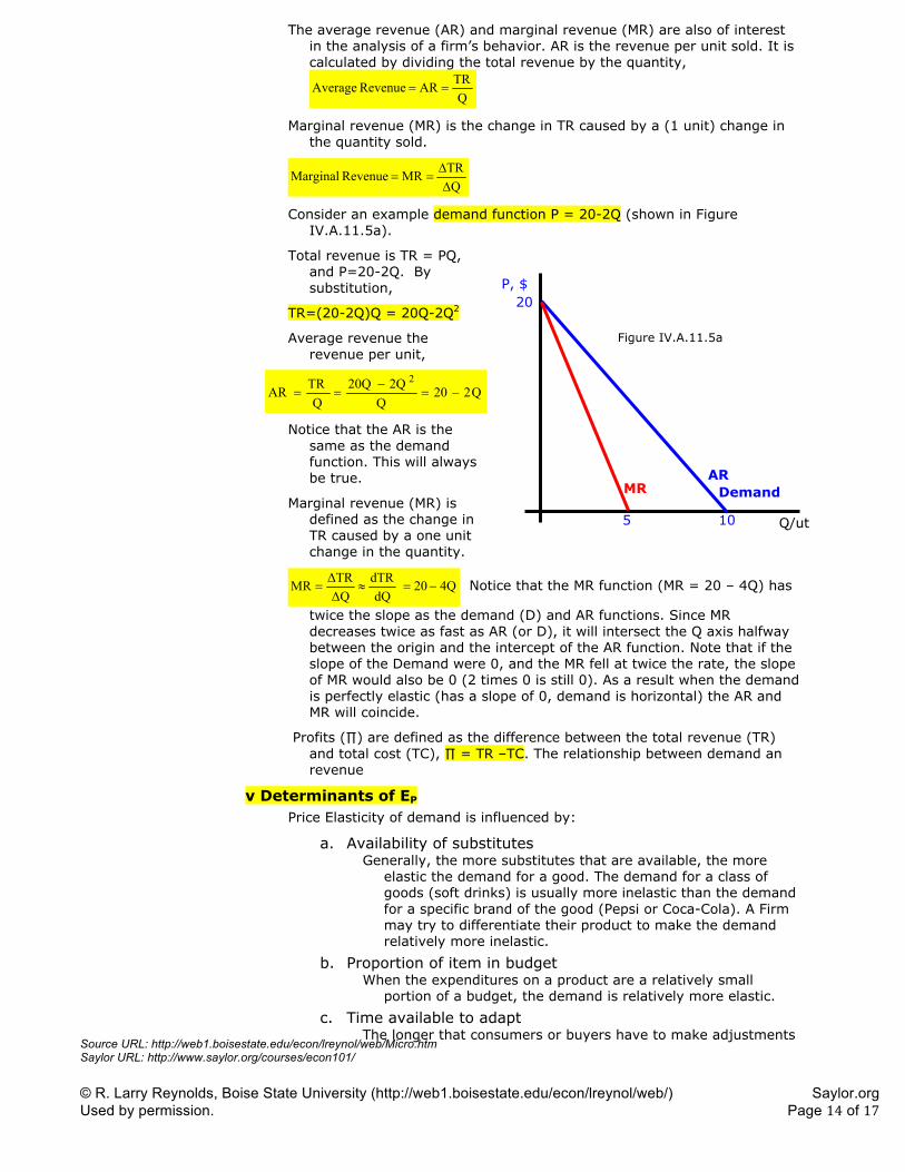
The average revenue (AR) and marginal revenue (MR) are also of interest in the analysis of a firm’s behavior. AR is the revenue per unit sold. It is calculated by dividing the total revenue by the quantity,

QTRARRevenueAverage

Marginal revenue (MR) is the change in TR caused by a (1 unit) change in the quantity sold.

QTRMRRevenue Marginal''

Consider an example demand function P = 20-2Q (shown in Figure IV.A.11.5a).

Total revenue is TR = PQ, and P=20-2Q. By substitution,

TR=(20-2Q)Q = 20Q-2Q2

Average revenue the revenue per unit,

Notice that the AR is the same as the demand function. This will always be true.

Marginal revenue (MR) is defined as the change in TR caused by a one unit change in the quantity.

4Q20dQ

dTRǻQǻTRMR � | Notice that the MR function (MR = 20 – 4Q) has

twice the slope as the demand (D) and AR functions. Since MR decreases twice as fast as AR (or D), it will intersect the Q axis halfway between the origin and the intercept of the AR function. Note that if the slope of the Demand were 0, and the MR fell at twice the rate, the slope of MR would also be 0 (2 times 0 is still 0). As a result when the demand is perfectly elastic (has a slope of 0, demand is horizontal) the AR and MR will coincide.

Profits (�) are defined as the difference between the total revenue (TR) and total cost (TC), � = TR –TC. The relationship between demand an revenue

v Determinants of EP Price Elasticity of demand is influenced by:

a. Availability of substitutes Generally, the more substitutes that are available, the more

elastic the demand for a good. The demand for a class of goods (soft drinks) is usually more inelastic than the demand for a specific brand of the good (Pepsi or Coca-Cola). A Firm may try to differentiate their product to make the demand relatively more inelastic.

b. Proportion of item in budget When the expenditures on a product are a relatively small

portion of a budget, the demand is relatively more elastic.

c. Time available to adapt The longer that consumers or buyers have to make adjustments

Q/ut

P, $

Demand

20

10 5

MR AR

Figure IV.A.11.5a



in their behavior, the more elastic the demand is likely to be. The absolute value of the short run price elasticity of demand for gasoline would be smaller than the absolute value of the long run price elasticity of demand. The longer time allows consumers more opportunity to adjust to price changes.

vi Interpretation of EP

Some examples of price elasticities of demand reported in Microeconomics for Today, [Tucker, p 123, South-Western College Publishing, 1999. Sources Archibald

and Gillingham, Houthakker and Taylor, Voith] are presented in Table IV.5. Note that the demand is relatively more elastic for longer periods. Some goods, like movies, are inelastic in the short run and elastic in the long run.

The coefficient or price elasticity can be used to estimate the percentage change in the quantity that consumers are willing and able to buy given a percentage change in the price. It is important to understand that this measure does not apply to the equilibrium conditions in the market.

In Table IV.5 the short run EP for gasoline is -.2. This suggests that a 1% increase in price will reduce the quantity demanded by .2%. A 10% decrease in price would increase the quantity demanded by 2%. In the case of movies, a 1% increase in the price would change the quantity demanded by 3.67% in the long run.

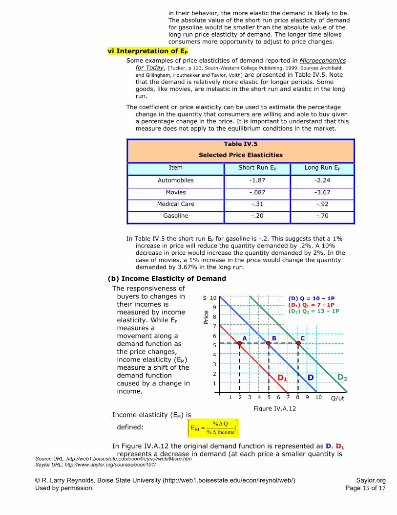
(b) Income Elasticity of Demand� The responsiveness of

buyers to changes in their incomes is measured by income elasticity. While EP measures a movement along a demand function as the price changes, income elasticity (EM) measure a shift of the demand function caused by a change in income.

Income elasticity (EM) is

defined: »¼

º«¬

ª{

Incomeǻ%Qǻ%

EM

In Figure IV.A.12 the original demand function is represented as D. D1 represents a decrease in demand (at each price a smaller quantity is

Table IV.5

Selected Price Elasticities

Item Short Run EP Long Run EP

Automobiles -1.87 -2.24

Movies -.087 -3.67

Medical Care -.31 -.92

Gasoline -.20 -.70

D D1 D2

Pric

e

Q/ut

$

1 2 3 4 5 6 7 8 9 10

1

2

3

4

5

6

7

8

9

10

A B C

Figure IV.A.12

(D) Q = 10 – 1P (D1) Q1 = 7 - 1P (D2) Q2 = 13 – 1P



purchased. When a larger quantity is purchased at each price, this will

represent an increase of demand to D2.

Given the original demand function (D), consumers are willing and able

to purchase 5 units of the good. If income increased by 50% and

“caused” the demand to shift to D2, where 8 units are purchased at

$5. This is a 60% increase in demand. Income elasticity (EM) is

calculated:

2.1%50%60

%%

� ��

''

MQ

E M

In this case, an increase in income resulted in an increase in demand. A

decrease in income might decrease the demand (to D1). In this case

income elasticity would be

2.1%50%60

%%

� ��

''

MQ

E M

When EM is positive, the good is called a normal good. If an increase in

income reduces demand (or a decrease in income increases demand),

EM will be negative and the good is categorized as an inferior good.

a. EM < 0 means the good is inferior, i.e. for an increase in income the

quantity purchased will decline or for a decrease in income the

quantity purchased will increase

b. 1 > (M> 0 means the good is a normal good, for an increase in

income the quantity purchased will increase but by a smaller

percentage than the percentage change in income.

c. For EM > 1 the good is considered a superior good.

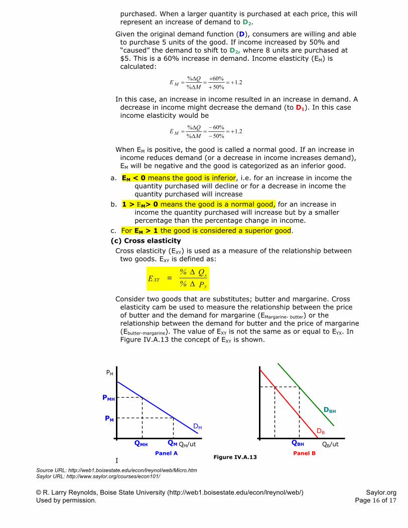
(c) Cross elasticity Cross elasticity (EXY) is used as a measure of the relationship between

two goods. EXY is defined as:

P %Q %

Ey

xXY '

'{

Consider two goods that are substitutes; butter and margarine. Cross

elasticity cam be used to measure the relationship between the price

of butter and the demand for margarine (EMargarine- butter) or the

relationship between the demand for butter and the price of margarine

(Ebutter-margarine). The value of EXY is not the same as or equal to EYX. In

Figure IV.A.13 the concept of EXY is shown.

I

Panel A Panel B Figure IV.A.13

QM/ut

PM

DM

QM

PM

PMH

QMH QB/ut

DB

QBH

DBH



In panel A, the demand for margarine (DM) is shown. At a price of PM, the quantity demanded is QM. In Panel B, the demand for butter (DB) is shown. At a price of PB, the quantity demanded is QB. If the price of margarine increased to PMH (in Panel A), the quantity of margarine demanded decreases to QMH. Since less margarine is purchased, the demand for butter increases to DBH (in Panel B). Given the higher demand for butter the butter demanded (given the higher price of margarine) has increased. A decrease in the price of margarine would shift the demand for butter to the left (decrease). The coefficient of cross elasticity would be positive.

In the case of complimentary goods, an increase (decrease) in the price of tennis balls would reduce (increase) the demand for tennis rackets. The coefficient of cross elasticity would be negative. If EXY is close to zero, that would be evidence that the two goods were not related. If EXY were positive or negative and significantly different from zero, it could be used as evidence that the two goods are related. It is possible that EXY might be positive or negative and the two goods are not related. The price of gasoline has gone up and the demand for PC’s has also increased. This does not mean that gasoline and PC’s are substitutes.

x� When (xy > 0, [a positive number] this suggests that the two goods are substitutes

x� When (xy < 0, [a negative number] this suggests that the two goods are compliments

(1) Elasticity and Buyer Response Elasticity is a convenient tool to describe how buyers respond to

changes in relevant variables. Price elasticity (EP) measures how buyers respond to changes in the price of the good. It measures a movement along a demand function. It is used to describe how much more of less the quantity demanded is as the price falls or rises.

Income elasticity (EM) is a measure of how much the demand function shifts as the income(s) of the buyer(s) changes. Cross elasticity (EXY) measures how much changes in the price of a related good will shift the demand function.

Elasticity can be calculated to estimate the relationship between any two related variables.

Documents

Chapter 9: Consumer Behavior