Embed Size (px)
Citation preview
Outline
Constrained Modern Floorplanning Problem (CMFP)
Bound-feasibility check BFS/IBFS/CBFS Algorithm Postprocessing Experimental Results
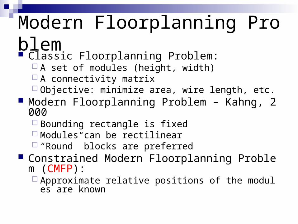
Modern Floorplanning Problem Classic Floorplanning Problem:
A set of modules (height, width) A connectivity matrix Objective: minimize area, wire length, etc.
Modern Floorplanning Problem – Kahng, 2000 Bounding rectangle is fixed Modules can be rectilinear “Round” blocks are preferred
Constrained Modern Floorplanning Problem (CMFP): Approximate relative positions of the modules are kno
wn
Design FlowBound
Feasi bl e?
Mi n-cost Max-fl owBased Fl oorpl anner
Postprocessi ng
Connected?
Suggesti ons
Yes
No
Yes
No
I nput
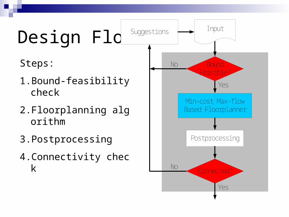
Steps:
1. Bound-feasibility check
2. Floorplanning algorithm
3. Postprocessing
4. Connectivity check
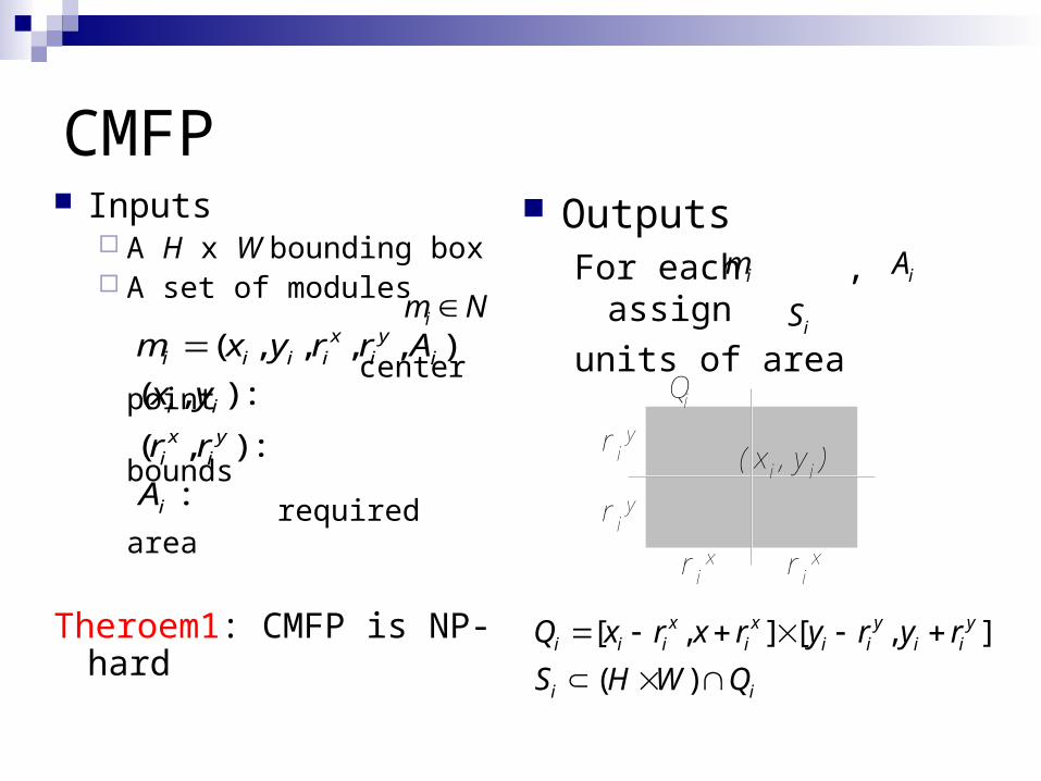
CMFP Inputs
A H x W bounding box A set of modules
center point bounds required area
Theroem1: CMFP is NP-hard
im N( , , , , )
( , ) :
( , ) :
:
x yi i i i i i
i i
x yi i
i
m x y r r A
x y
r r
A
(xi , yi )
Qi
r ix r i
x
r iy
r iy
OutputsFor each , assign
units of areaim iA
[ , ] [ , ]
( )
x x y yi i i i i i i i
i i
Q x r x r y r y r
S H W Q
iS

Bound-Feasibility
Bound-Feasibility: N is the set of modules, for any subset T of N
( )i i
i im T m T
A Area Q
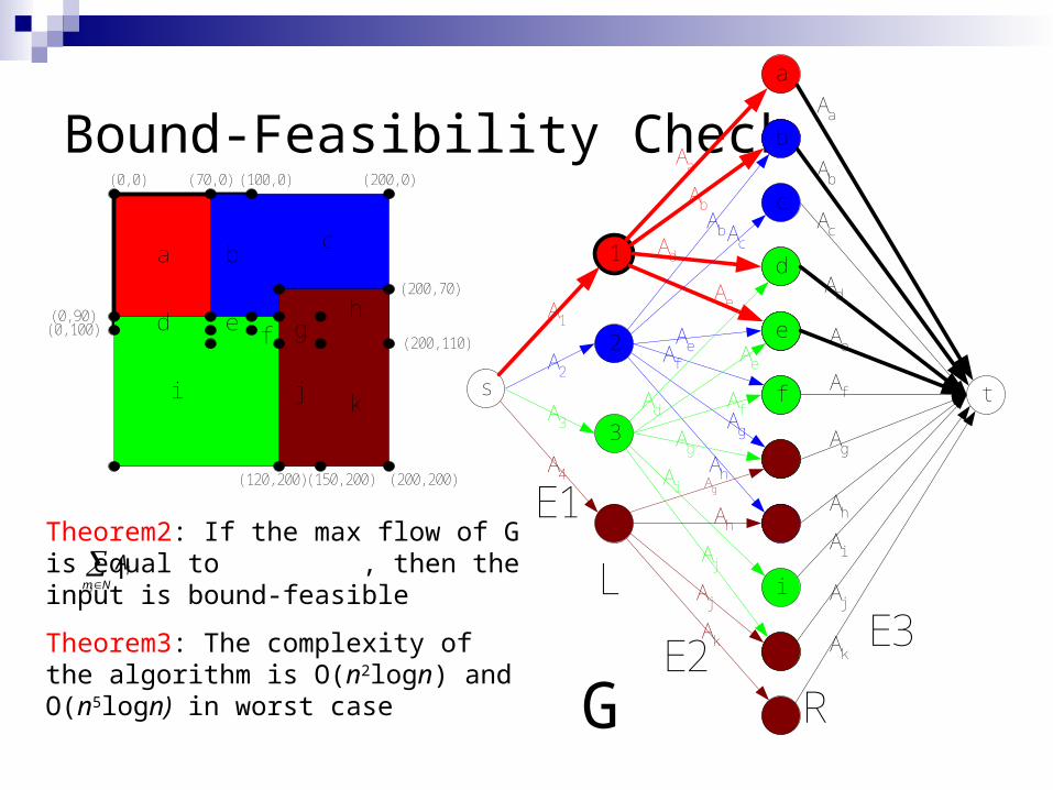
Bound-Feasibility Check
1 2
3 4
(0, 0) (70, 0) (100, 0) (200, 0)
(200, 70)
(0, 90)(0, 100)
(200, 110)
(200, 200)(150, 200)(120, 200)
a b
d ef g
h
i jk
c
gg
e
d1
2
3
4
a
b
c
d
e
f
g
h
i
j
k
b
s
e
f
h
j
t
Aa
A2
A3
A4
Ab
Ad
Ae
Aa
A1
Ab
Ac
Ad
Ae
Af
Ag
Ah
Ai
Aj
Ak
AbAc
AeAf
Ag
Ah
Ad
Ae
Af
Ag
Ai
Aj
Ag
Ah
Aj
Ak
R
L
E1
E2E3
Theorem2: If the max flow of G is equal to , then the input is bound-feasible
Theorem3: The complexity of the algorithm is O(n2logn) and O(n5logn) in worst case
i
im N
A
G

Min-Cost Max-Flow Algorithm
Problem: A module could be assigned to regions that are not adjacent.
Solution: A min-cost max-flow algorithm Maintaining maximum flow of G, Minimize , where ce is the cost assigned to
the edge of G, fe is the flow of e. This encourages assigning the connected regions to a module.
2
e ee E
c f
2e E
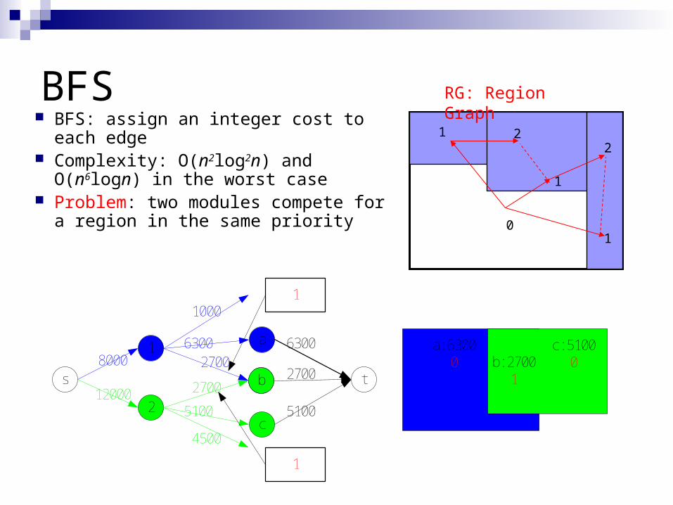
BFS BFS: assign an integer cost to each edge Complexity: O(n2log2n) and O(n6logn) in
the worst case Problem: two modules compete for a
region in the same priority
a
c
1
2
bs b t8000
12000
6300
2700
5100
63002700
2700
5100
1 2a: 6300
0 b: 27001
c: 51000
1000
4500
1
1
0
2
1
1
21
RG: Region Graph
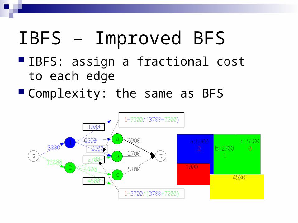
IBFS – Improved BFS IBFS: assign a fractional cost to each
edge Complexity: the same as BFS
c
e1
2
e
bs
a
b t8000
12000
6300
2700
5100
63002700
2700
5100
12
a: 63000 b: 2700
1
c: 51000
1000
4500
1+7200/ (3700+7200)
1+3700/ (3700+7200)
31000
44500
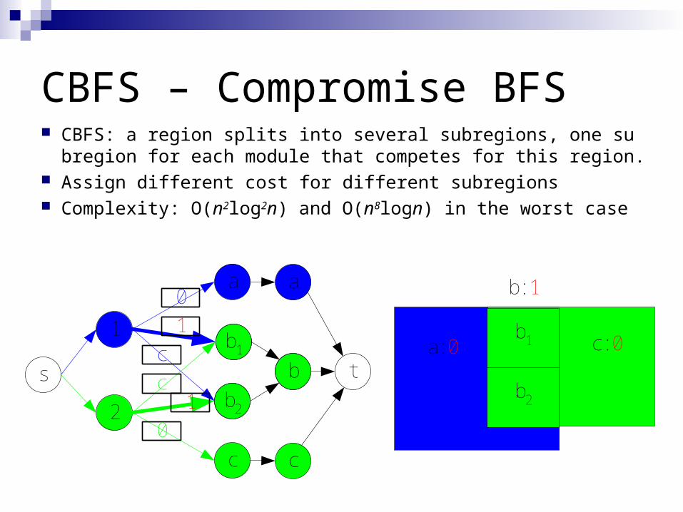
CBFS – Compromise BFS
b2
c
a
1
2
b1
s
b1
t 1 2a: 0 c: 0
b2b2
b1
0
cc
0
1
1
b: 1a
bb
c
CBFS: a region splits into several subregions, one subregion for each module that competes for this region.
Assign different cost for different subregions Complexity: O(n2log2n) and O(n8logn) in the worst case
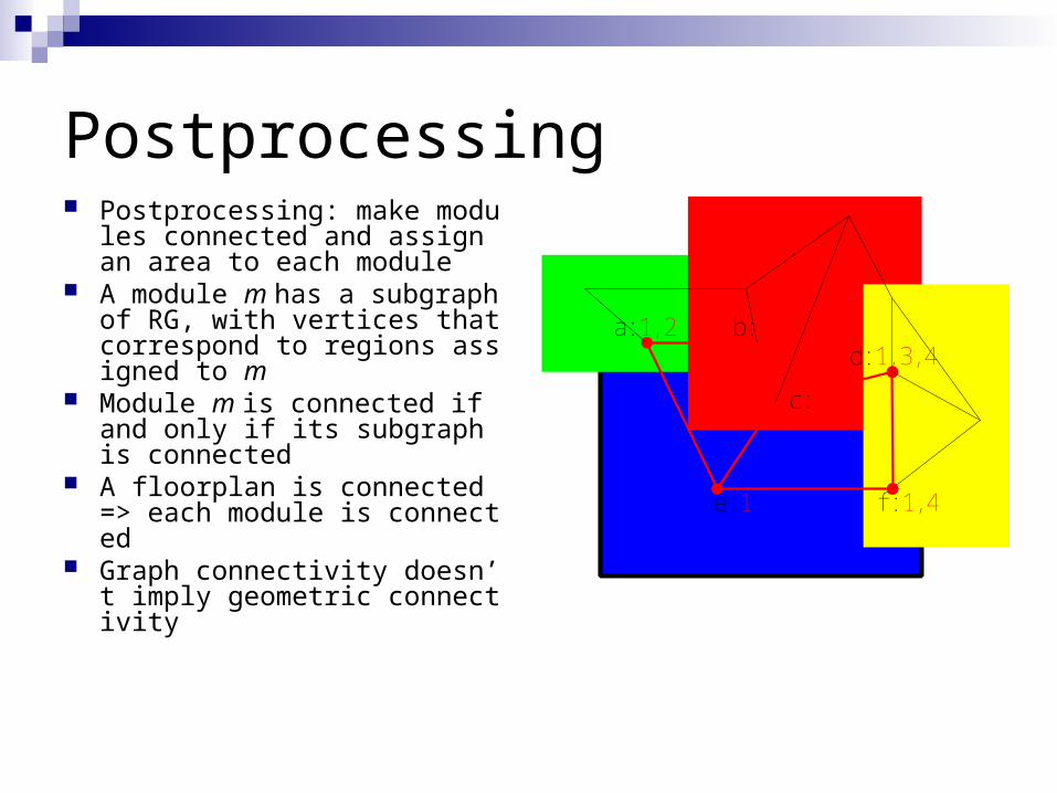
Postprocessing Postprocessing: make module
s connected and assign an area to each module
A module m has a subgraph of RG, with vertices that correspond to regions assigned to m
Module m is connected if and only if its subgraph is connected
A floorplan is connected => each module is connected
Graph connectivity doesn’t imply geometric connectivity
1
2 3
4
a: 1, 2 b: 1, 2, 3
c: 1, 3
d: 1, 3, 4
e: 1 f : 1, 4
Experiments
Implementations: Java and C++ Benchmarks: ami33, ami49 and n300a An initial step to obtain initial module
positions
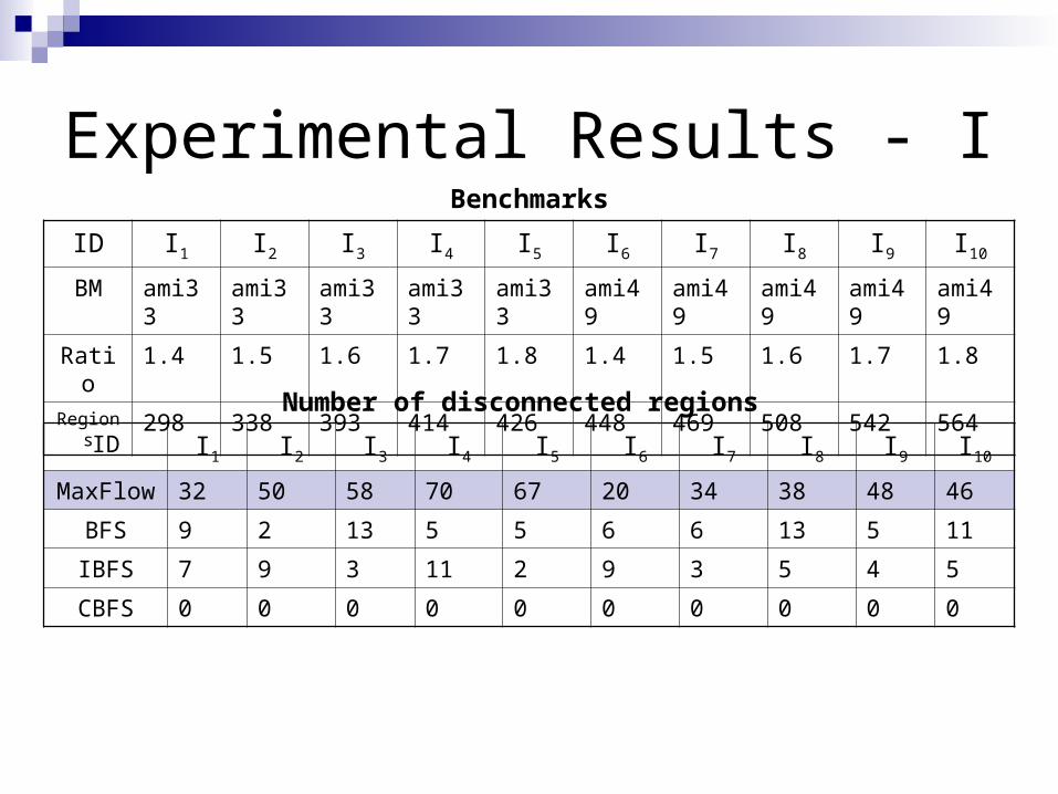
Experimental Results - I
ID I1 I2 I3 I4 I5 I6 I7 I8 I9 I10
BM ami33 ami33 ami33 ami33 ami33 ami49 ami49 ami49 ami49 ami49
Ratio 1.4 1.5 1.6 1.7 1.8 1.4 1.5 1.6 1.7 1.8
Regions 298 338 393 414 426 448 469 508 542 564
Benchmarks
ID I1 I2 I3 I4 I5 I6 I7 I8 I9 I10
MaxFlow 32 50 58 70 67 20 34 38 48 46
BFS 9 2 13 5 5 6 6 13 5 11
IBFS 7 9 3 11 2 9 3 5 4 5
CBFS 0 0 0 0 0 0 0 0 0 0
Number of disconnected regions
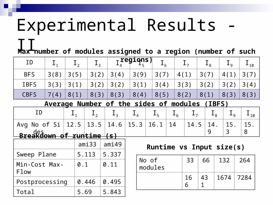
Experimental Results - II
ID I1 I2 I3 I4 I5 I6 I7 I8 I9 I10
BFS 3(8) 3(5) 3(2) 3(4) 3(9) 3(7) 4(1) 3(7) 4(1) 3(7)
IBFS 3(3) 3(1) 3(2) 3(2) 3(1) 3(4) 3(3) 3(2) 3(2) 3(4)
CBFS 7(4) 8(1) 8(3) 8(3) 8(4) 8(5) 8(2) 8(1) 8(3) 8(3)
Max number of modules assigned to a region (number of such regions)
ID I1 I2 I3 I4 I5 I6 I7 I8 I9 I10
Avg No of Sides 12.5 13.5 14.6 15.3 16.1 14 14.5 14.9 15.3 15.8
Average Number of the sides of modules (IBFS)
ami33 ami49
Sweep Plane 5.113 5.337
Min-Cost Max-Flow 0.1 0.11
Postprocessing 0.446 0.495
Total 5.69 5.843
Breakdown of runtime (s)
No of modules 33 66 132 264
166 431 1674 7284
Runtime vs Input size(s)

ENDThank you!