daSilva2009

8/6/2019 daSilva2009

http://slidepdf.com/reader/full/dasilva2009 1/27

Conceptual Flexible Aircraft Model for Modeling,

Analysis and Control Studies

Andre Luıs da Silva,∗ Pedro Paglione† and Takashi Yoneyama‡

Technological Institute of Aeronautics (ITA), S˜ ao Jose dos Campos, SP, 12228-900, Brazil

In this paper, we present models of conceptual flexible aircraft suitable for aerodynamic,flight mechanics and flight control studies. The aircraft is representative of a medium sizecivil jet transport and it is developed in three configurations of increasing flexibility. Themodel integrates 6 degrees of freedom rigid and structural dynamics, which are obtainedvia finite elements and mo dal decomposition (up to 9 flexible modes are considered). Anincremental unsteady aerodynamic model is determined via the Doublet Lattice method.The aircraft possesses 8 aerodynamic control effectors, suitable for control of the rigidand flexible modes. A rigid body aerodynamic model is also considered. A brief numericdiscussion about flutter is also presented.

I. Introduction

Every aircraft is, in fact, a flexible body and its motion should be evaluated by the mechanic of continuousbodies. However, an aircraft is commonly treated, in the flight mechanics, as a rigid body. In other way,in the structural dynamics, the rigid body modes are commonly neglected. Such separation is acceptablewhen there is sufficient separation between rigid and flexible modes natural frequencies. However, trends incivil transport aircraft industry are leading to aircrafts with longer fuselages, larger aspect ratios, smallerthicknesses, composite material structures (characteristics that are already present in some unmanned air-craft, such as the NASA Helios aircraft). These configurations lead to aircrafts that are more flexible thanusual, so the flexible and rigid body modes natural frequencies tend to approximate, and integrated models

for flight mechanics and structural dynamics need to be considered.One of the earlier works in the flight mechanics of flexible aircraft is due to Milne (1964).1 In this

work, the concept of mean axis reference frame (MRF) is introduced, in order to promote inertial decouplingbetween rigid and flexible modes; the steady strip theory is applied to determine the incremental aerodynamicloads due to flexibility; the structural dynamics is determined by tension-deformation relationships in controlpoints and displacements compatibility. The approach is applied to the longitudinal dynamics. In Dusto etal. (1974),2 the MRF is chosen to write the equations of motion, while the aerodynamic frame is chosen towrite the aerodynamic forces. In Cavin and Dusto (1977),3 the Hamilton principle is invoked to determinethe motion equations, the MRF is considered and the structural dynamics is modeled via finite elements.In Karpel (1981),4 unsteady aerodynamics via rational function approximation (RFA) is adopted, and aprocedure to include traditional control and stability derivatives in the RFA is presented.

In Waszak and Schmidt (1988),5 under some assumptions, the coincidence between the MRF and theusual rigid body attached frame (RBRF) is considered; the equations of motion are derived via the Lagrange

formalism; the structural dynamics is represented via the modal decomposition; the incremental aerodynam-ics is determined via the quasi steady strip theory for the longitudinal dynamics. The major contributionis a flexible aircraft flight mechanics model that extends the traditional rigid body model, with flexible andrigid body dynamics connected only via incremental aerodynamic forces and moments and generalized forcesin the flexible modes. The same methodology is found in Ref. 6. In Buttrill et al. (1987),7 the MRF andthe RBRF are considered distinct, the similarity with the rigid body models is lost. It is shown that the

∗Doctorate Student, Electronic Engineering Division, Systems and Control, [email protected]†Professor Associado, Aeronautical Engineering Division, Flight Mechanics, [email protected]‡Professor Titular, Electronic Engineering Division, Systems and Control, [email protected]

1 of 27

American Institute of Aeronautics and Astronautics

8/6/2019 daSilva2009


inertial coupling is important for low aerodynamic loads, or angular speeds in the order of flexible modesfrequencies. In Waszak et al. (1992),8 a comparison between the approaches in Refs 5 and 7 is performed.

In Vink and de Jonge (1997),9 a longitudinal model of a simple flexible aircraft is presented. Theaerodynamic loads are determined via non steady strip theory, with the Theodorsen function; 10 the structuresof wing and fuselage are approximated by beam elements and assumed modes are adopted.

In Meirovitch and Tuzcu (2004),11 the equations of motion are derived in the RBRF without consideringit coincident to the MRF. Two groups of equations are determined: nonlinear equations for the rigid bodymotion and linear equations for the structural model. The structural model is called delta model and

determines the influence of the flexible modes in the rigid body states.In Reschke (2006),12 the inertial coupling between rigid and flexible modes is discussed again, and the

conclusions are similar to those in Ref. 7. The structure is represented via lamped masses. The DoubletLattice method is applied to determine unsteady aerodynamic increments due to structural motion.

In Silvestre and Paglione (2008),13 the strip theory is applied to expand the formulation of Ref. 5 for thecomplete aircraft dynamics (longitudinal and lateral directional). It is also presented a numerical evaluationthat supports the coincidence of the RBRF and MRF under some hypothesis. In Silvestre and Luckner(2009),14 another strip theory approach is presented, however, for the unsteady case. In Pogorzelski etal. (2009),15 another approach via unsteady strip theory is applied to compute the aerodynamic loads inthe formulation of Ref. 5. In Neto (2008),16 the Doublet Lattice method is applied to determine theseaerodynamic loads, also for unsteady flow.

In general, the formulations presented above involve nonlinear rigid body equations of motion and linearstructural dynamics, suitable for small structure displacements. Developments in the field of nonlinearstructural dynamics can be found in Ref. 17.

There are also works that discuss thrust effects in the flexible modes and the non existence of the elasticaxis (considered in some of the references above), Refs 18 and 19, respectively.

Concerning flexible aircraft flight control, in McLean (1978),20 optimal control and algebraic theory of model following control are applied to alleviate the effects on both the dynamic and structural responses of an aircraft flying through atmospheric turbulence. In Kubica et al. (1995),21 a formulation based on optimalcontrol and eigenstructure assignment is applied to control law design of a flexible aircraft with significantcoupling between rigid and flexible modes dynamics. In Livet et al. (1995),22 a robust control methodologybased in quadratic programming is also applied to control law design of a flexible aircraft with significantcoupling between rigid and elastic modes. In Joshi and Kelkar (1996),23 robust control is applied to thelongitudinal dynamics of a flexible aircraft, taking the structural dynamics as uncertainty.

In Aouf et al. (2000, 2001, 2002),24–27 a series of works discussing the application of robust control

techniques to flexible aircraft are presented. The applications include vertical acceleration control via H 2,weighted-H 2 and H ∞ approaches in the presence of flexible modes; model reduction via µ synthesis, withtruncation of flexible modes; and gain scheduling of controllers designed via frozen H ∞ for flexible aircraft.

In Alazard (2002),28 control augmentation system for the lateral dynamics of a flexible aircraft is devel-oped in two steps: assurance of performance and robustness with respect to flexible modes for the rigid bodydynamics; guarantee of damping in the flexible modes.

In Meirovitch and Tuzcu (2004),11 an approach for the suppression of the effect of flexible modes inthe rigid body variables is presented. First, the rigid body model is considered independent of the deltadynamics. Then, the delta model is controlled via LQR, taking in to account the dependence with rigidbody variables, in order to guarantee the former assumption.

Other control applications to flexible aircrafts can be found in Refs 29–32, all relying on robust controltheory. Some concerning artificial intelligence can be found in Refs. 33 and 34.

In numerical applications of approaches developed for incremental aerodynamic loading computation in

flexible aircrafts, a model of the structural dynamics is necessary, as well as various aircraft data, such asgeometry. In other way, to perform control applications, a model that integrates the rigid and flexible bodyaerodynamics, structure dynamics and inertias is necessary. To acquire a model for the first application is notan easy task; one can be found, for example, in an aeronautical industry, as performed in the developmentof the model in Ref. 15 (though some models can also be found in the open literature). In the second case,it is more common to find models in the open literature.

Concerning the discussion above, in the Ref. 5, a model is given for the longitudinal dynamics of theB1 Lancer with 4 structural modes, determined according the formulation presented therein. In Waszaket al. (1987),35 data for both longitudinal and lateral directional dynamics of this aircraft are presented,

2 of 27


8/6/2019 daSilva2009


however, only for two flexible modes. In this article, the modal forms of these vibration modes and therespective geometric grid are also presented that enables the application of some formulations for incrementalaerodynamic loading evaluation. For example, the applications in Refs 36 and 16 are fed with these data.Another reference that presents structural dynamics data is Ref. 9. In this case, one can find a simple modelfor the longitudinal dynamics of a conceptual aircraft, with structural dynamics evaluated representing thewing and fuselage structures by beam elements and taking assumed modes. Such formulation is suitable forparticular strip theory applications.

In Ref 28, linear models of the lateral-directional dynamics of a flexible aircraft, suitable for control

applications, are presented. The model data are not included in the paper. Instead, the electronic addressof a repository where they can be found is given. The models possess 18 flexible modes and considerunsteady aerodynamics. In Ref 20, a linear model for the longitudinal and lateral directional dynamics of the B52 bomber, suitable for control applications, is presented, with 5 symmetrical and 5 anti-symmetricalmodes. In ref 37, a MATLAB/Simulink package is described that implements a model of a high speed civiltransport (HSCT) flexible aircraft with 6 DOF rigid body nonlinear equations and 40 structural modes, withdynamics represented via modal decomposition. In this model, the rigid body aerodynamics are obtained inwind tunnel and the incremental aerodynamics due to flexible modes is determined via elastic-to-rigid ratiosin the aerodynamic database.

In this paper, we present a model of flexible aircraft suitable for control applications, that can also beapplied in incremental aerodynamic loading determination and open loop simulations and analysis. Wedevelop a conceptual design of a medium size civil jet in the class of Boeing 737-200/300 and EmbraerERJ190/195. Three configurations with increasing flexibility are developed. For the first configuration, weconsider 8 flexible modes and, for the others, 9. In each configuration, there are 8 aerodynamic controleffectors suitable to control all the flexible modes.

The models are developed according the formulation presented in Ref. 5, with incremental unsteadyaerodynamics determined via the Doublet Lattice method application presented in Ref. 16, extended inorder to compute the influence of the control surfaces in the flexible modes. The structural dynamics isdetermined via modal decomposition evaluated via finite elements with the software NASTRAN. The rigidbody aerodynamics and mass distributions are determined using the AAA software that implements aircraftconceptual design approaches presented in Ref. 38.

We present a rigid body 6 DOF aerodynamic model, an unsteady incremental aerodynamic model, aswell as mass, inertias and structure dynamics data; giving complete information for control applications(naturally, the models also can be applied in open loop simulations and analysis). We also make availablethe modal forms of each flexible mode of each configuration and the respective geometrical grids, that can

be applied in incremental aerodynamic loading computation.Open loop poles are presented with a brief discussion on the occurrence of flutter flutter.

II. Theoretical Background

A flexible aircraft is a continuous body with an infinity number of degrees of freedom. In this case,continuum mechanics should be applied to study the respective dynamics, which involves, in the Lagrangianformalism, for example, to write a Lagrangian density function which leads to partial differential equations. 39

The approach applied in this paper, however, is much more simple and extends the rigid body flight mechan-ics. The formulation is presented in Ref. 5 and combines rigid body mechanics and mechanics of continuousbodies discretized as a finite arrangement of elements. Such discretization is well known in the dynamics of structures field and can be performed via, for example, finite elements.40

In the following, first, we present the technique applied to describe structural dynamics, which is composed

by discretization and modal decomposition. After, we present the development of the general equations of motion for a flexible aircraft. Finally, we present an unsteady aerodynamic formulation via the DoubletLattice method to compute aerodynamic loading in a flexible aircraft.

II.A. Structural Mechanics

Consider a continuous structure discretized in n control points. According Ref. 41, taking into accountsmall displacements, the position of any point in the structure can be written as a linear combination of the

3 of 27


8/6/2019 daSilva2009


positions of the control points, as in Eq. 1.

p(x, y, z, t) = N(x, y, z)q(t) (1)

q(t) = [q1(t) q2(t) q3(t) . . . q3n−2(t) q3n−1(t) q3n(t)]T

(2)

In Eq. 2, qi+1(t), qi+2(t) and qi+3(t) are the displacements, in some chosen Cartesian reference frame, inthe axes x, y and z, respectively, of such frame, with respect to an equilibrium position, of the ( i

−1)th control

point of the discretization in some time instant t. In the study of the displacements with respect to someinertial system of reference attached to an equilibrium state of the structure, the variables qj , j = 1, 2, . . . , 3n,are generalized coordinates.

In Eq. 1, p(x, y, z, t) is the displacement, with respect to an equilibrium position, in the chosen referenceframe, of a generic point in the continuous body, identified by coordinates x, y and z, in some time instantt. N(x, y, z) is a matrix operator dependent on the position of the generic point. Equation 1 states aninterpolation of the particular displacements in q(t) to generate a generic displacement p(x, y, z, t).

A continuous body can be discretized in a variety of ways, for example, via concentrate or finite elements.Given some discretization approach, the geometry of the body, the properties of its materials, the constraintsof one body section with respect to each other and with the external environment, one can write the bodykinetic energy with respect to the reference system chosen to evaluate the structure deformation, the potentialenergy due to elastic deformation and the structure dissipation function, as a function of the generalized

coordinates qj . In the case of small displacements and respective rates, these functions are linear with respectto the generalized coordinates and time rates.41 These functions are presented in Eq. 3.

T e =1

2qT Mq, U e =

1

2qT Kq, F = 1

2qT Bq (3)

where T 2 is the kinetic energy due to structure deformation, U e is the elastic potential energy and F isthe dissipation function. M, K and B are the mass, stiffness and damping matrices, respectively. Thesematrices are dependent in the properties discussed above (discretization, material properties, etc). A varietyof Engineering softwares exist to compute them, for example, MSC NASTRAN R.

Once a set of generalized coordinates and the expressions for the kinetic and potential energy and dissi-pation function are written with respect to them, the Lagrangian formalism can be applied, which leads tothe following equations of motion:

Mq + Bq + Kq = Q (4)

where Q is a vector of generalized forces.Taking, in Eq. 4, B = 0 and Q = 0 one obtains the so called undamped free vibration problem:

Mq + Kq = 0. The respective solutions possess important properties applicable to the general case. Infact, supposing that the solution of this simplified problem is given by q(t) = q0ePt, where q0 is a constantvector and P is a constant scalar to be determined, the following eigenvalue problem follows:

(K− λM)q0 = 0, λ = −P 2 (5)

The solution of the eigenvalue problem is given by 3n eigenvalues λi real and positive and 3n eigenvectorsΣi.

41 These eigenvalues define 3n natural frequencies ωni =√

λi, and the eigenvectors define deformationpatterns, named modal forms, for the undamped free vibration problem. Each pair (ωni , Σi) defines a freevibration mode of the structure and a given set of such pairs is called modal basis.

According Ref. 41, the modal eigenvectors have the following orthogonality properties with respect to

the mass and stiffness matrices:

ΣT i MΣj = 0 and ΣT

i KΣj = 0, f or λi = λj

ΣT i MΣj = 0 and ΣT

i KΣj = 0, f or λi = λj

i, j = 1, 2, . . . 3n (6)

The properties in Eq. 6 can be applied to simplify the general vibration problem in Eq. 4 as follows.Let us define the transformation:

q(t) = Ση, Σ = [Σ1 Σ2 . . . Σ3n], η(t) = [η1(t) η2(t) . . . η3n(t)]T (7)

where ηi(t), i = 1, 2, . . . 3n are functions to be determined.

4 of 27


8/6/2019 daSilva2009


Inserting q(t) given by Eq. 7 in the Eq. 4, applying the orthogonality properties in Eq. 6, and performingsome algebraical manipulations, the general equations of motion reduce to:

ηi + 2ζ iωni ηi + ω2niηi =

ψi

µi, i = 1, 2, . . . 3n (8)

where ωni are the free vibration modes frequencies, µi = ΣT i MΣi are called generalized masses, ζ i are called

generalized dampings, and ψi are new generalized forces.In fact, in order to obtain the result in equation 8, it is necessary the additional hypothesis that ΣT BΣ

is a diagonal matrix. According Ref. 41, this matrix is not necessarily diagonal. However, as the dampingmatrix B, in aeronautical structures, has relatively small terms, it is reasonable to approximate the productin question as diagonal.

According Eqs. 8 and 7, the displacements of the structure can now be described by the new set of variables η1, η2, . . . η3n. So, this is a new set of generalized coordinates for the structural dynamics. Thesenew coordinates are called modal amplitudes. They are dimensionless variables that determine the truedisplacements of the control points via the transformation in Eq. 7, which is called modal transform .

With the new generalized coordinates, T e, U e and F are given by:

T e =1

2

3ni=1

µiη2i , U e =

1

2

3ni=1

µiω2niη2i , F = 1

2

3ni=1

2µiζ iωni η2i (9)

II.B. General Equations of MotionIn order to develop the aircraft equations of motion, it is necessary to choose systems of reference andrespective reference frames. An inertial reference system is mandatory, for this purpose, as in the rigid bodyflight mechanics, we consider that the earth surface behaves as such, and take it as the inertial referencesystem. We choose also the usual inertial reference frame (IRF) of rigid body flight mechanics, with x0 andy0 axes parallel to the earth surface and z0 axis towards its center.

As in rigid body flight mechanics, it is important to consider the body itself as a system of reference andsome respective reference frames. As in Ref. 5, we choose the following body reference frames:

• Rigid body reference frame (RBRF), that is the traditional body reference frame of rigid body flightmechanics, with x axis parallel to the undeformed aircraft symmetric axis and towards the nose; zaxis perpendicular to x, contained in the undeformed aircraft longitudinal symmetry plane, towardsthe aircraft floor; y axis completing the dextrorotatory coordinate system. The origin is fixed to the

undeformed aircraft center of gravity;

• The aerodynamic reference frame (ARF), identical to the one in rigid body flight mechanics, that isdefined almost identically to the RBRF, with the difference that the ARF x axis is oriented in thedirection of the aircraft center of gravity velocity;

• The mean axis reference frame (MRF), that is not necessarily attached to physical points in the body,but it is defined via the Eq. 10.

V

dp

dt

MRF

ρdV = 0,

V

p× dp

dt

MRF

ρdV = 0 (10)

In the Eq. 10, p is the position vector of a mass element in the body with respect to the MRF, writtenin the MRF; the subindex MRF indicates that the vector derivatives are taken with respect to the MRF;and the integral shall be determined along the entire volume of the body.

In Ref. 5, the flexible aircraft equations of motion are determined via the Lagrange formalism, that isbased in the Euler-Lagrange equation:

d

dt

∂L

∂ qk

− ∂L

∂qk+

∂ F ∂ qk

= Qk, k = 1, 2, . . . N (11)

where qk is a set of generalized coordinates; L is the Lagrangian , that is the difference between the kineticand potential energies L = T − U ; F is the dissipation function; and Qk are generalized forces, that aregiven by equation 12.

Qk =

V

f · ∂ pi

∂qkdV (12)

5 of 27


8/6/2019 daSilva2009


where f is the aerodynamic and thrust forces by volume along the aircraft.In order to evaluate the Euler-Lagrange equations, it is necessary to determine the kinetic energy with

respect to the inertial reference system, the potential energy and the dissipation function.The aircraft kinetic energy is given by:

T =1

2

V

dpi

dt· dpi

dtρdV (13)

where pi is the position of a body mass element in the IRF and the derivative is computed with respect tothis coordinate system.If R0 is the position of the origin of the MRF with respect to the IRF, pi is given by

pi = R0 + p (14)

Taking the relationship between the time derivative of a vector in coordinates systems that rotate withrespect to each other,39 from the equation 14, we have that:

dpi

dt=

dR0

dt+

dp

dt

MRF

+ω × p (15)

where ω is the angular velocity of the MFR with respect to the IRF.From Eqs. 15 and 14, we have that:

T =1

2

V

dR0

dt·

dR0

dtρdV +

1

2

V

(ω × p) · (ω × p) ρdV +1

2

V

dp

dt

MRF

·dp

dt

MRF

ρdV +

V

dR0

dt·

dp

dt

MRF

ρdV +

V

dR0

dt· (ω × p) ρdV +

V

dp

dt

MRF

· (ω × p) ρdV (16)

As demonstrated in Ref. 5, the properties in equation 10 imply that the 4th and the 6th integral in theright hand side (rhs) of equation 16 are zero. Also, taking the origin of the MRF coincident with the aircraftinstantaneous center of gravity, the 5th integral is also zero.

The first integral in the rhs of eq. 16 is the translational kinetic energy of the aircraft center of gravity,the second is the kinetic energy due to rotation, the third is the kinetic energy due to structure deformation.As in Ref. 5, considering that the structure deformation do not change the aircraft inertia tensor, the secondintegral leads to the same result of the rotational kinetic energy of a rigid body. Also, adopting the structural

mechanics approach of subsection II.A, with kinetic energy due to structure deformation given by Eq. 9, wehave that the aircraft total kinetic energy is given by:

T =1

2m(u2 + v2 + w2) +

1

2ωT Iω +

1

2

3ni=1

µiη2i (17)

where m is the aircraft mass; u, v and w are the components, in the axis x, y and z of the MRF, respectively,of the velocity of the instantaneous aircraft center of gravity with respect to the IRF; ω = [ p q r]T is therotational velocity of the MRF with respect to the IFR written in the MRF; I is the inertia tensor withrespect to the MFR; ηi are the modal amplitudes of the structure, for a discretization in n control points,with modal forms written in the MRF.

The advantage of consider the MFR is to obtain, in Eq. 17, inertial decoupling between rigid and flexiblebody terms. However, the main problem is that, the speeds u, v and w, the rates p, q and r, the inertia

tensor and the modal forms shall be written in the MFR. So, the the meaning of this variables may becomedifficult to understand due the abstract nature of the MRF. This problem is solved, in an approximatedway, in Ref. 5. Under the following hypotheses: structural displacements collinear to the respective timederivatives; deformations that do not change the center of gravity positions, nor the mass elements densities;it is shown that the MFR and RBRF are coincident. So, all the definitions in Eq. 17 and in the discussionthat follows are identical to the rigid body case, as both coordinate systems can be used without distinction.

The hypotheses above are reasonable for small deformations, aerodynamic surfaces reasonably moreflexible than the fuselage and fuselage mass considerably greater than aerodynamic surfaces masses. For anaircraft with such characteristics, in the Ref. 13, it is shown, in a numeric application, that the MFR andthe RBRF are really almost coincident.

6 of 27


8/6/2019 daSilva2009


The potential energy is the sum of the gravitational and the elastic potential energies:

U = −mg (−xcg sin θ + ycg sin φ cos θ + zcg cos φ cos θ) +1

2

3ni=1

µiω2ni

η2i (18)

where g is the acceleration due to gravity; xcg, ycg and zcg are the components, in the axes of the RBRF, of the position of the aircraft center of gravity with respect to the IRF; φ, θ and ψ are the Euler angles of theRBFR with respect to the IRF.

The dissipation function is given by Eq. 9.

F = 1

2

3ni=1

2µiζ iωni η2i (19)

Adopting the generalized coordinates xcg, ycg, zcg, φ, θ, ψ and ηi, i = 1, 2, . . . 3n, we can apply the Euler-Lagrange equations and the integral form of the generalized forces (Eq. 12) to determine the equations of motion of the flexible aircraft. However, in the equation 17, the potential energy is not written in functionof them. But, using the well known relationships:

p = φ− ψ sin θ, q = θ cos φ + ψ cos θ sin φ, r = ψ cos φ cos θ − θ sin φ (20)

u = xcg + qzcg − rycg, v = ycg + rxcg − pzcg, w = zcg + pycg − qxcg (21)

and performing a sort of algebraical manipulations, we obtain a set of motion equations for the flexibleaircraft similar to the rigid body case, with 3 equations for translation, 3 for rotation and 3 n for structuralmechanics. However, we obtain translation equations written in function of u, v and w, that is not soconvenient for flight control. Taking, however, one more step, and transforming the translational equationsfrom the RBRF to the ARF, via relationships given by the matrix of coordinates transformation betweenthese two frames, we obtain these equations in function of the center of gravity speed V , angle of attack αand sideslip angle β. So, we get this final set of equations of motion for the flexible aircraft:

V =T

mcos α cos β − D

m+ g(sin φ cos θ sin β + cos φ cos θ sin α cos β − cos α cos β sin θ) (22)

α = q

− p cos α tan β

−r sin α tan β

−L

mV cos β

+g

V cos β

(cos φ cos θ cos α + sin α sin θ) (23)

β = p sin α− r cos α +Y

mV − T

mV sin β cos α +

g

V cos β(sin φ cos θ + sin θ sin β cos β cos α +

− sin φ cos θ sin2 β − cos φ cos θ sin α sin β cos β) (24)

˙ p =

I yyI zz − I 2zz − I 2xz

qr + (I xzI zz − I xzI yy + I xxI xz) pq + I zzL+ I xz N

I xxI zz − I 2xz(25)

q =I xzr2 + (I zz − I xx) pr − I xz p2 +M+MT

I yy(26)

r = (I xzI yy − I xzI zz − I xxI xz) qr +

I 2xz + I

2xx − I xxI yy

pq + I xzL+ I xx N

I xxI zz − I 2xz(27)

ηi + 2ζ iωiηi + ω2i ηi =

Qηi

µi, i = 1, 2, . . . nm (28)

Equations 22 to 27 are the well known rigid body equations of translational and rotational Dynamics.Equation 28 contains the structural dynamics equations presented in subsection II.A. To complete the motionequations, it is necessary to add the Kinematic equations. The rigid body kinematic equations are the well

7 of 27


8/6/2019 daSilva2009


known ones from the rigid body flight dynamics. Kinematic translational equations are given in Eqs 29 to31, the rotational ones are given in Eqs 32 to 34.

x0 =((sin(β) sin(φ) + sin(α) cos(β) cos(φ)) cos(ψ) sin(θ) + cos(α) cos(β) cos(ψ) cos(θ)+

(sin(α)cos(β) sin(φ)− sin(β) cos(φ)) sin(ψ))V (29)

y0 =((sin(β) sin(φ) + sin(α) cos(β) cos(φ)) sin(ψ) sin(θ) + cos(α) cos(β) sin(ψ) cos(θ)+

(sin(β) cos(φ)− sin(α) cos(β) sin(φ)) cos(ψ))V (30)

H =− ((sin(β) sin(φ) + sin(α)cos(β)cos(φ))cos(θ)− cos(α) cos(β) sin(θ))V (31)

φ = p + (q sin φ + r cos φ)tan θ (32)

θ =q cos φ− r sin φ (33)

ψ =r cos φ sec θ + q sin φ sec θ (34)

In Eqs. 22 to 24, T , D, L and Y are thrust, drag, lift and side forces, respectively. In equations 25 to 27,L, M and N are the aerodynamic rolling, pitching and yawing moments, respectively; MT is the pitchingmoment due to thrust. In Eq. 28, Qηi is the generalized force in the ith vibration mode.

In Eq. 28, the generalized forces can be determined via the following integral:

Qηi =

V

f ·ΦidV (35)

where Φi is the modal form Σi interpolated along any point of the structure.In Eqs 29 to 31, x0 and y0 are the coordinates of the aircraft cg in the axes x and y of the IRF, H = −z0

is the aircraft altitude, where z0 is analogous to x0 and y0.In Eq. 28, it shall be noted that the index i extends until nm and not 3n. Since the modes of vibration

possess frequencies of increasing order,41,42 after a given amount of modes, say nm, the respective frequenciesmay be very large compared to the rigid body natural frequencies, such that they can be neglected, as highorder dynamics.

The Eqs 25 to 27 are determined with the additional hypothesis of a symmetric aircraft: I xy = I yz = 0.At a first glance, the rigid and elastic body equations of motion appear uncoupled. However, it is

necessary to determine T , L, D, Y , MT , L, M, N and Qηi taking into account that the aircraft is a flexiblebody. So, coupling may appear via forces and moments in the rigid body dynamics and generalized forcesin the flexible modes. The determination of these forces, moments and generalized forces is discussed in the

next subsection.

II.C. Aerodynamic Model

In this subsection, we discuss the determination of the forces T , L, D and Y , moments MT , L, M and N and generalized forces Qi, in a flexible aircraft.

As performed in the Refs 5, 36 and 16, we consider that the thrust T and the pitching moment due tothrust MT are not affected by the flexibility. So, they can be determined by usual rigid body approaches.

In the determination of aerodynamic forces and moments, as performed in Refs 5, 36 and 16, we considersmall structure displacements such that the aerodynamic is linear, with the forces and moments given bythe sum of some increments to the respective values in the rigid body:

L = L + ∆L, D = D + ∆D, Y = Y + ∆Y, L = L+ ∆L, M = M+ ∆M, N = ¯ N + ∆ N (36)

where L, D, Y , L, M and ¯ N are the lift, drag, side-force and aerodynamic pitching, rolling and yawingmoments in the rigid body. ∆L, ∆D, ∆Y , ∆L, ∆M and ∆ N are the lift, drag, side-force and aerodynamicrolling, pitching and yawing moments increments due to structure deformation.

The rigid body aerodynamic forces and moments can be determined via usual rigid body techniques.In order to determine their increments due to structure deformation, as well the generalized forces in theflexible modes (GFFM), we adopt an unsteady aerodynamic approach based in the Doublet Lattice method,presented in the Ref. 16.

In the following, first we present a synthesis of the approach in Ref. 16 for the computation of incrementalforces and moments. After, we present a synthesis of the approach in Ref. 16 for the determination of GFFMwith a brief extension to include control surface effects.

8 of 27


8/6/2019 daSilva2009


II.C.1. Incremental Aerodynamic Forces and Moments

The Doublet Lattice method is a linear approach in unsteady aerodynamics where compressibility effects aretaken into account (in the absence of nonlinear effects, such as shock waves).

The method is elaborated in the frequency domain taking into account harmonic variations in time(s = iω). The development of the method results in an equation that relates the speed normal to a surface,with the difference of pressure coefficients, via the following integral:

ˆw =w(x, y, z)

V ∞

=1

8π

SSK (x− ξ, y − η, z − ζ , ω , M )∆C p(ξ, η, ζ )dξdη (37)

where V ∞ is free stream speed, w is the speed normal to the surface in the frequency domain (in this

development, the accent ˆ indicates a variable in the frequency domain); ∆C p is the difference of pressurecoefficients in the surface in the frequency domain; ξ, η and ζ = ζ (ξ, η) are the coordinates of the points of the aerodynamic surface SS that influence the normal speed in the point of coordinates x, y and z. Thefunction K , named kernel function, depends on the relative position between (x, y, z) and (ξ, η, ζ ), the freestream Mach number M and the frequency ω of the harmonic motion.

Using discretization via panels and considering that the integration of the kernel function, in the directionof the free stream flow (ξ) is concentrated along a line in the quarter chord of a panel, the integral in Eq.37 reduces to:

ˆw(x, y, z) = S

∆C ps∆ξ

8π S K (x− ξ1/4, y − η, z − ζ , ω , M )dη (38)

where the index s indicate all the panels that influence the normal speed in (x, y, z). The elements char-acterized by (ξ, η, ζ ) are named sending elements, while the elements characterized by (x, y, z) are namedreceiving elements.

In Eq. 38, the normal speed in the point (x, y, z) is known because it corresponds to the boundarycondition of the problem, while the difference of pressure coefficients is unknown. Such equation can bewritten as:

ˆw

= D

∆C p

(39)

The matrix D is a square matrix of influence coefficients, represented by induced downwash factors duethe sending element s, in the receiving element r.

In order to the matrix D be square, the number of receiving and sending elements shall be the same.For this purpose, a receiving element is associated to each panel in the discretization and a coordinate is

given to it, called a control point, which is the point where the boundary condition is taken. The optimumposition of such point is 3/4 of the mean chord of each panel.

Once the panel discretization is defined, the matrix D is determined for a given Mach number andfrequency. A MATLAB code to compute the D matrix was implemented by the author of Ref. 16.

Once the matrix D is known, it is possible to determine the pressure difference in the sending element of each panel, in the frequency domain, given that the normal speeds in each receiving element is known.

For small deformations, using linearization, it is shown that the normal speed is given by:

wj =∂hj

∂t+ V ∞

∂hj

∂x(40)

where hj is the displacement normal to the surface in the receiving element j due to flexibility.There are considered only structural displacements normal to the aerodynamic surfaces, what is rea-

sonable for small deformation of wings and empennages and it is according the hypothesis presented in

subsection II.B, for the coincidence of the MRF and RBRF. The displacement h can be obtained via themodal transformation in the Eq. 7, taking only the components of the modal forms normal to each surface.

Taking the Laplace transform to wj in the Eq. 40, for harmonic temporal variations, dividing the resultby V ∞, and performing some arrangements, the vector of normal speeds is given by:

ˆw

=

ik(·) +

∂

∂ x(·)

ˆh

(41)

where k = ωb/V ∞ is named reduced frequency (dimensionless), b is a reference length (that is taken equalto half of the wing mean aerodynamic chord: b = cw/2), hj = hj/b and x = x/b.

9 of 27


8/6/2019 daSilva2009


So, the pressure coefficient difference in the panel j is given by:

∆C p,j = AIC( j, :)

ˆw

(42)

where AIC = D−1 is another matrix of influence coefficients and AIC( j, :) is its line j.

Given the vector

∆C p

, the incremental lift, side-force and incremental aerodynamic moment with

respect to an axis π are given by:

∆L

= qdSL

∆C p

,

∆Y

= qdSY

∆C p

,

∆M π

= qdSM

∆C p

, SM = dc/4,π (SL + SY ) (43)

In Eq. 43, SL is a diagonal matrix with the areas of each panel, in the case of surfaces with horizontalplanform, and zeros for vertical planform surfaces. SY is also a diagonal matrix, with the areas of eachpanel, for vertical planform surfaces, and zeros for horizontal planform surfaces. dc/4,π is a diagonal matrixwith the distances of the points in the 1/4 mean chord of each panel with respect to the axis π, π = x, y, z(incremental moments ∆L, ∆M, ∆ N ), multiplied by the respective signal according the convention for thesignal of the moment, or zero, if the axis is parallel to the panel normal. Also, qd is the dynamic pressure.

The incremental induced drag is not covered by the Doublet Lattice method. In the Ref. 16, an approachinvolving the vortex lattice method was developed for this purpose. In a numeric evaluation, it is shownthat the influence of this incremental force in the aircraft dynamics is very small, while the computationaleffort and formulation complexity increases in significance. By this reason, in the development in question,

we neglect the incremental induced drag.The incremental forces and moments in Eq. 43 are determined in the frequency domain. In the following,it is presented a formulation to obtain them in the time domain. First, let us condensate Eq. 43 as:

[∆χ] = qdSχAIC

ˆw

, χ = L, Y,M π (44)

Applying the Eq. 7 in Eq. 41, after some algebraical manipulations, we have that:

ˆw

=

ik

Φ

+∂

∂ x

Φη (45)

where Φ is a matrix of interpolated modal forms in the panels control points, divided by the reference lengthb. An element at line j and column k is the modal displacement at the control point of panel j due to thevibration mode k. The vector η is the Laplace transform of the vector of modal amplitudes.

From Eqs 44 and 45, we have that:

[∆χ] = qdSχAIC

ik

Φ

+∂

∂ x

Φη (46)

In order to transform the equation 46 from the frequency to the time domain, we take the Laplacetransform. However, the matrix AIC is determined for a single frequency and taking into account s = iω.In order to enable the transformation for the time domain, it is adopted a fitting for the following matrix:

Q(ik) = AIC

ik

Φ

+∂

∂ x

Φ

(47)

The matrix in Eq. 47 assumes a particular result for each frequency ik. A fitting approach consists in

the determination of a matrix that is function of s = σ + iω, from a particular set of matrices¯Q(ik). Thematrix adopted is presented in Eq. 48. Such approach is named rational function approximation (RFA).

Qap = Q0 + Q1s

b

V ∞

+ Q2s2

b

V ∞

2

+

nlagi=1

sQ2+n

s + (V ∞/b)βn(48)

In the Eq. 48, Qn are constant matrices to be determined, s is the Laplace variable, βn are called lagterms and nlag is the number of lag terms.

In the Ref. 16, a least squares approach is adopted to fit the matrices Qn in Eq. 48, for a given Machnumber, from a set of matrices Q(ik) determined for a given set of reduced frequencies k. The author of

10 of 27


8/6/2019 daSilva2009


Ref. 16 also developed a MATLAB code to implement this approach. The code determines the matrices Qn,given that the lag terms βn and its amount are already specified. The parameters βn may be determinedvia optimization, or arbitrated via the analyst experience.

Once the approximation in Eq. 48 is performed, the Eq. 46 is written in function of the Laplace variables, that is continuous and valid for any temporal variation:

[∆χ] = qdSχ Q0 + Q1sb

V ∞ + Q2s2b

V ∞2

+

nlag

i=1

sQ2+n

s + (V ∞/b)βn η (49)

In Ref. 16, it is shown that the inverse Laplace transform of the Eq. 49 is given by:

[∆χ] = qdSχ

Q0η + Q1

b

V ∞

η + Q2

b

V ∞

2

η +

nlagn=1

Q2+nηlag,n

, χ = L, Y, M π (50)

ηlag,n = η − V ∞b

βnηlag,n, n = 1, 2, . . . nlag (51)

In Eq. 51, each element of the vector ηlag,n is named lag state. This equation shows that the DoubletLattice unsteady approach adds nm × nlag first order linear differential equations to the motion equations.

After some algebraical manipulations, the incremental aerodynamic forces and moments can be writtenvia derivatives of influence coefficients, analogous to traditional stability derivatives:

∆L =1

2ρV 2S w

C Lηk ηk + C Lηn

lagk

ηnlagk +cw

2V ∞C Lηk ηk +

c2w4V 2∞

C Lηkηk

(52)

∆Y =1

2ρV 2S w

C Y ηk ηk + C Y ηn

lagk

ηnlagk +cw

2V ∞

C Y ηk ηk +c2w

4V 2∞

C Y ηk ηk

(53)

∆L =1

2ρV 2S wbw

C lηk ηk + C lηn

lagk

ηnlagk +cw

2V ∞C lηk ηk +

c2w4V 2∞

C lηk ηk

(54)

∆M =1

2ρV 2S w cw

C mηk

ηk + C mηnlagk

ηnlagk +cw

2V ∞C mηk

ηk +c2w

4V 2∞

C mηkηk

(55)

∆ N =

1

2 ρV

2

S wbw

C nηk ηk + C nηnlagk η

n

lagk +

cw

2V ∞C nηk ηk +

c2w

4V 2∞C nηk ηk

(56)

where S w is the wing planform area, cw is the wing mean aerodynamic chord, bw is the wing span and ρ isthe air density. The reference length was taken equal to cw/2.

In Eqs 52 to 56, the Einstein notation is adopted, where the repetition of indices denotes summation.The wing area, wing span and wing mean aerodynamic chord where inserted in order to obtain dimensionlesscoefficients. The definition of such coefficients is straightforward from the Eq. 50.

II.C.2. Generalized Forces in the Flexible Modes

For the determination of the generalized forces in the flexible modes, the integral in Eq. 12 is considered.So, we have to determine the aerodynamic and propulsive forces by volume along the aircraft. For thisdevelopment, the following assumptions are taken: instead of consider forces by volume, we consider forcesby area, as in the Doublet Lattice method the forces are taken along surfaces; the propulsive effects areneglected, as the propulsive forces are distributed in a relatively small area and the pylons, generally, havelarge stiffness; only force distributions along the the wing and empennages are considered, since the fuselage,nacelles and pylons generate relatively small aerodynamic forces and possess greater stiffness.

From the assumptions above, the generalized forces can be computed via the following relationship:

Qηi =

Sw,ht

σzφzi dS +

Svt

σyφyi dS (57)

In Eq. 57, the index S w,ht means that the integral shall be evaluated along the wing and horizontal tailsurfaces, analogously, the index S vt indicates that the integral shall be evaluated along the surface of the

11 of 27


8/6/2019 daSilva2009


vertical tail. σz is the aerodynamic force by area in the z direction of the RBRF, φzi is the interpolated

modal displacement due to the ith vibration mode in the z direction of the RBRF, σy and φyi are analogous

to σz and φzi taking into account the y direction of the RBRF.

The notation and development in question can be simplified considering that σn is the aerodynamic forceby area normal to an aerodynamic surface, with the signal given by the positive direction of the RBFRparallel to this normal. Analogously, φn

i is the interpolated modal displacement normal to an aerodynamicsurface, with the same convention of signal. With these definitions, Eq. 57 can be written as:

Qηi = S

σnφni dS (58)

where the index S indicates that the integral shall be evaluated along all the aerodynamic surfaces.Approximating the integral in Eq. 58 by a summation along the panels of Doublet Lattice discretization,

we have that:Qηi =

j

σnjφnij

S j =j

F njφnij (59)

In the Eq. 59, the summation shall be taken along all the panels. S j is the area of the jth panel. σnj is themean normal force by area in the jth panel and φn

ijis the normal modal displacement in a control point of

the jth panel (it is chosen the same control point adopted in the Doublet Lattice formulation). Also, F nj isthe normal aerodynamic force in the jth panel.

Once again, we consider linear aerodynamics such that F nj can be given as the sum of its value in the

rigid body and an increment due to the flexibility.F nj = F nj + ∆F nj (60)

In the Eq. 60, F nj is the force in panel j in the rigid body and ∆F nj is its increment due to flexibility.The increment ∆F n,j can be directly determined from the Eq. 50. Considering small angle of attack and

sideslip angle, we can approximate:

F nj = −1

2ρV 2S L( j,j)

Q0( j, :)η + Q1( j, :)

b

V ∞

η + Q2( j, :)

b

V ∞

2

η +

nlagi=1

Q2+n( j, :)ηlag,n

(61)

for panels in the wing and horizontal tail,

F nj =1

2ρV 2S Y ( j,j)

Q0( j, :)η + Q1( j, :)

b

V ∞η + Q2( j, :)

b

V ∞2

η +

nlag

i=1Q2+n( j, :)ηlag,n

(62)

for panels in the vertical tail.The rigid body force distribution F nj can be obtained via an aerodynamic panel method developed for

the rigid body case. In this situation, we can use steady aerodynamics as in the Vortex Lattice method.An implementation of the Vortex Lattice method is described in the Ref. 43. The implementation is calledTornado, it is developed in MATLAB and can determine rigid body aerodynamic forces distribution asfunction of angle of attack, angle of sideslip, angular rates, control surface deflections and reference state.The implementation is based also in linear aerodynamics.

Defining a reference state, for example α = β = p = q = r = 0, with also all the control deflections equalto zero (that we call null reference state), we can use a method like that implemented in Tornado to derive,via finite differences, the force distribution F nj as the following linear combination:

F nj = F 0nj + F αnjα + F βnjβ + F pnj p + F qnjq + F rnjr + F δknj δk (63)

In Eq. 63, F 0nj is the normal force in the panel j in the null state. F xnj is the derivative of F nj withrespect to the variable x, determined via finite differences in the null state. δk is the deflection of the controlsurface δk. In the last term in the rhs, once again, the notation of Einstein is applied.

Collecting the results in Eqs 59, 60, 61, 62 and 63 and performing some algebraical manipulations, wecan write the generalized forces in the flexible modes as:

Qηi =1

2ρV 2S w cw

C ηi0 + C ηiαα + C ηiβ β + C ηiηk

ηk + C ηiηnlagk

ηnlagk +cw

2V ∞

C ηiq q + C ηiηk

ηk

+ (64)

bw2V ∞

C ηip p + C ηir r

+

c2w4V 2∞

C ηiηkηk + C ηiδk

δk

12 of 27


8/6/2019 daSilva2009


In the Eq. 64, again, the Einstein notation is used. Also, the reference length was taken equal to cw/2.Moreover, the definition of coefficients therein requires some algebra, but is straightforward.

As in the determination of incremental aerodynamic forces and moments, the generalized forces in theflexible modes are given in function of derivatives of influence coefficients. Such derivatives can be seen asan extension of the traditional stability and control derivatives of rigid body mechanics.

III. Conceptual Aircraft Model

In this section, we present a model of a conceptual flexible aircraft. We have developed a conceptualdesign for a civil jet similar to Boeing 737-200/300 and Embraer ERJ 190/195. This conceptual aircraftpossesses 3 variants of increasing flexibility: configuration 1 (conf1) of standard flexibility; configuration 2(conf2) of augmented flexibility; configuration 3 (conf3) of high flexibility.

In the following, first, we describe the general characteristics of the conceptual aircraft and present arigid body aerodynamic model. After, we discuss the structural arrangement, considered in a finite elementsapplication for determination of a modal basis, and present structure dynamics data, as well as aircraftinertias. Finally, we present an incremental aerodynamic model for the aircraft.

III.A. Conceptual Aircraft General Presentation and Rigid Body Aerodynamic Model

The conceptual aircraft was conceived via historical data of the following similar aircrafts: Embraer ERJ-190/195, Boeing 737-200/300, Douglas DC-9-S80, Douglas DC-9-50, Fokker F-28-4000, British AircraftCorporation BAC-1-11-495, British Aerospace BAe-146-200. Data and general configuration of these similaraircraft were applied to support definition of independent parameters and general configuration. These datawere also applied to determine dependent parameters via geometrical relationships and conceptual designapproaches. For some calculations, the AAA R software, that implements the aircraft conceptual designmethods present in Ref. 38, was adopted.

The 3 aircraft variants possess the general configuration: low wing with trapezoidal planform. Fuselagemounted horizontal tail (ht), with trapezoidal planform. Fuselage mounted vertical tail (vt), with trapezoidalplanform. Two jet engines under the wing. Cylindrical fuselage.

The general control surfaces arrangement, common for the 3 variants, is composed as follows: two aileronwith symmetric and anti-symmetric deflection, one inboard and one outboard. This has been shown asnecessary to control both symmetric and anti-symmetric modes in the wing. Two elevators in the horizontaltail, one inboard and one outboard. The inboard elevator is conceived for rigid body control. The outboard

elevator is proposed for symmetric flexible modes control. Two rudders in the vertical tail, one lower andone upper. The lower rudder is conceived for rigid body control. The upper rudder is suggested for anti-symmetric flexible modes control.

In order to define this control surface arrangement, some controllability analyses with respect to theflexible modes were performed. We applied a constrained controllability approach presented at Ref. 44.They are not presented in this paper.

In table 1, general parameters are presented. In table 2, control surfaces geometrical parameters, thatare the same for the 3 variants, are presented. In table 3, the aerodynamic surfaces profiles are presented.

The main differences between the three aircraft variants are the aerodynamic surfaces aspect ratios andthicknesses. Table 1 shows that wing, horizontal tail and vertical tail aspect ratios where increased fromconf1 to conf3. Also, table 3 shows that the thicknesses of these surfaces where decreased from conf1 to conf3.These changes increase the aircraft flexibility from conf1 to conf3. In the aerodynamic and performance pointof view, such modifications contribute to reduce the drag and increase the fuel efficiency.

For the 3 aircraft variants, we determine a rigid body aerodynamic model, given by stability and controlderivatives. These models are given for the flight condition: altitude H = 10000m; M = 0.75, V ∞ =224.6m/s; α = β = 0; p = q = r = 0. To compute the data, the AAA and the Tornado softwares were used.

The following conventions are adopted: lift L, drag D and side-force Y positive in the sense of −z, −xand y in the AFR. Moments L, M and N positive in the directions x, y and z of the RBRF. Angular rates

p, q and r positive in the directions x, y and z of the RBRF. Anti-symmetric δaa and symmetric δas ailerondeflections positive according the right-hand rule (rhr) with hinge line (hl) in the direction of the right semiwing. Elevator deflections δe positive according the rhr with hl in the direction of the right side of horizontaltail. Rudder deflections δr positive according the rhr with hl in the direction of the vertical tail tip.

13 of 27


8/6/2019 daSilva2009


The system of units is the SI. So, angles are given in radians and angular rates in radians by second.The rigid body stability and control derivatives are presented in tables 4 and 5. The rigid body aerody-

namic forces and moments are given, in function of them, via the following equations:

L =1

2ρV 2S w

C L0

+ C Lαα +

cw2V ∞

C Lqq + C Lαα

+ C Lδei δei + C Lδeo δeo + C Lδasi

δasi + C Lδasoδaso

D =

1

2 ρV 2

S w

C D0 + C Dαα +

cw2V ∞C Dqq + C Dδei δei + C Dδeoδeo + C Dδasiδasi + C Dδasoδaso

Y =

1

2ρV 2S w

C Y ββ +

bw2V ∞

C Y p p + C Y rr + C Y β β

+ C Y δaai δaai + C Y δaaoδaao + C Y δrl δrl + C Y δru δru

L =1

2ρV 2S wbw

C lββ +

bw2V ∞

C lp p + C lrr + C lβ β

+ C lδaai δaai + C lδaaoδaao + C lδrl δrl + C lδru δru

M =1

2ρV 2S wcw

C m0

+ C mαα +

cw2V ∞

C mq

q + C mαα

+ C mδeiδei + C mδeo

δeo + C mδasiδasi + C mδaso

δaso

¯ N =1

2ρV 2S wbw

C nββ +

bw2V ∞

C np p + C nrr + C nβ β

+ C nδaai δaai + C nδaaoδaao + C nδrl δrl + C nδru δru

(65)

Par. Description conf1 conf2 conf3

l Aircraft length 33m 33m 33m

rf Fuselage cross section radius 1.5m 1.5m 1.5m

S w Wing planform area 95m2 95m2 95m2

Aw Wing aspect ratio 8.5 10 12

bw Wing span 28.4m 30.8m 33.8m

cw Wing mean aerodynamic chord 3.67m 3.38m 3.09m

Λc/4w Wing quarter chord sweep angle 25o 25o 25o

λw Wing taper ratio 0.3 0.3 0.3

Γw Wing dihedral 0 0 0

iw Wing incidence angle 3o 1o 1o

zw Distance from wing 1/4 root chord to the fuselage cross section center −0.75m −0.75m −0.75mS h Horizontal tail planform area 26m2 26m2 26m2

Ah Horizontal tail aspect ratio 5 6 7.6

bh Horizontal tail span 11.4m 12.5m 14.1m

ch Horizontal tail mean aerodynamic chord 2.43m 2.18m 1.94m

Λc/4h Horizontal tail quarter chord sweep angle 27.5o 27.5o 27.5o

λh Horizontal tail taper ratio 0.45 0.45 0.45

Lh Distance from ht aerodynamic center to aircraft cg along fuselage axis 15m 15m 15m

Γh Horizontal tail dihedral 0 0 0

ih Horizontal tail incidence angle 0 0 0

zh Distance from ht 1/4 root chord to the fuselage cross section center 0.75m 0.75m 0.75m

S v Vertical tail planform area 20m

2

20m

2

20m

2

Av Vertical tail aspect ratio 1.5 2 2.5

bv Vertical tail span 5.48m 6.32m 7.07m

cv Vertical tail mean aerodynamic chord 3.79m 3.28m 2.93m

Λc/4v Vertical tail quarter chord sweep angle 40o 40o 40o

λv Vertical tail taper ratio 0.5 0.5 0.5

Lv Distance from vt aerodynamic center to aircraft cg along fuselage axis 13.5m 13.5m 13.5m

Table 1. General parameters of the three variants.

14 of 27


8/6/2019 daSilva2009


Parameter Value Description

dwt−at 0 Distance from the outboard aileron tip until the wing tip

ba/bw 0.3 Total ailerons to wing span ratio

bai/ba 0.6 Inboard to total ailerons span ratio

bao/ba 0.4 Outboard to total ailerons span ratio

dhtt−et 0 Distance from the outboard elevator tip until the horizontal tail tip

be/beht 1 Total elevator to exposed horizontal tail span ratio

bei/be 0.6 Inboard elevator to total elevator span ratiobeo/be 0.4 Outboard elevator to total elevator span ratio

dvtt−rt 0 Distance from the upper rudder tip until the vertical tail tip

br/bvt 1 Total rudder to vertical tail span ratio

brl/br 0.6 Lower rudder to total rudder span ratio

bru/br 0.4 Upper rudder to total rudder span ratio

Table 2. Control surface data.

Surface conf1 conf2 conf3

Wing NACA 2412 NACA 2410 NACA 2408

Horizontal tail NACA 0010 NACA 0008 NACA 0006

Vertical tail NACA 0010 NACA 0008 NACA 0006Table 3. Aerodynamic surfaces profiles of the three variants.

= 0 α α β β p q r

conf1

C L 0.382 6.29 4.04 0 0 0 14.6 0

C D 0.0252 0.201 0 0 0 0 0.281 0

C Y 0 0 0 −0.785 0.0214 −0.0794 0 0.572

C l 0 0 0 −0.121 0.0035 −0.522 0 0.254

C m 0.0622 −3.63 −16.5 0 0 0 −45.5 0

C n 0 0 0 0.174 0.0098 −0.0587 0 −0.277

conf2

C L 0.296 7.23 4.92 0 0 0 17.4 0

C D 0.0217 0.207 0 0 0 0 0.174 0

C Y 0 0 0 −0.893 0.0197 −0.0778 0 0.626

C l 0 0 0 −0.133 0.0032 −0.558 0 0.228

C m 0.0407 −4.55 −21.9 0 0 0 −61.4 0

C n 0 0 0 0.207 0.0084 −0.0474 0 −0.278

conf3

C L 0.323 7.98 5.94 0 0 0 21.3 0

C D 0.0217 0.21 0 0 0 0 0.176 0

C Y 0 0 0 −1.01 0.018 −0.0918 0 0.668

C l 0 0 0 −0.16 0.0029 −0.588 0 0.245

C m 0.0515 −6.06 −29 0 0 0 −86.3 0

C n 0 0 0 0.233 0.007 −0.0546 0 −0.264

Table 4. Rigid body stability derivatives.

15 of 27


8/6/2019 daSilva2009


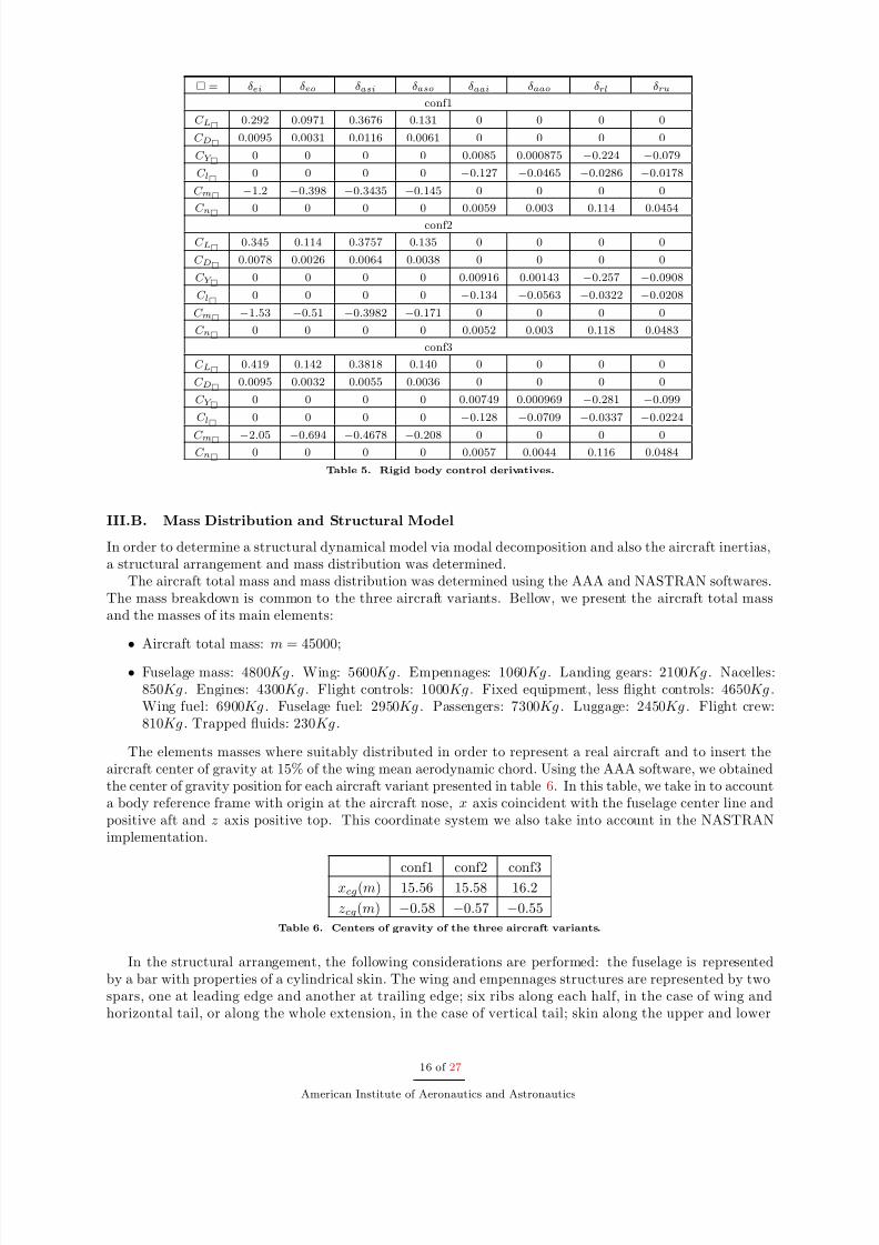
= δei δeo δasi δaso δaai δaao δrl δru

conf1

C L 0.292 0.0971 0.3676 0.131 0 0 0 0

C D 0.0095 0.0031 0.0116 0.0061 0 0 0 0

C Y 0 0 0 0 0.0085 0.000875 −0.224 −0.079

C l 0 0 0 0 −0.127 −0.0465 −0.0286 −0.0178

C m −1.2 −0.398 −0.3435 −0.145 0 0 0 0

C n 0 0 0 0 0.0059 0.003 0.114 0.0454

conf2

C L 0.345 0.114 0.3757 0.135 0 0 0 0

C D 0.0078 0.0026 0.0064 0.0038 0 0 0 0

C Y 0 0 0 0 0.00916 0.00143 −0.257 −0.0908

C l 0 0 0 0 −0.134 −0.0563 −0.0322 −0.0208

C m −1.53 −0.51 −0.3982 −0.171 0 0 0 0

C n 0 0 0 0 0.0052 0.003 0.118 0.0483

conf3

C L 0.419 0.142 0.3818 0.140 0 0 0 0

C D 0.0095 0.0032 0.0055 0.0036 0 0 0 0

C Y 0 0 0 0 0.00749 0.000969 −0.281 −0.099

C l 0 0 0 0 −0.128 −0.0709 −0.0337 −0.0224

C m −2.05 −0.694 −0.4678 −0.208 0 0 0 0C n 0 0 0 0 0.0057 0.0044 0.116 0.0484

Table 5. Rigid body control derivatives.

III.B. Mass Distribution and Structural Model

In order to determine a structural dynamical model via modal decomposition and also the aircraft inertias,a structural arrangement and mass distribution was determined.

The aircraft total mass and mass distribution was determined using the AAA and NASTRAN softwares.The mass breakdown is common to the three aircraft variants. Bellow, we present the aircraft total massand the masses of its main elements:

•Aircraft total mass: m = 45000;

• Fuselage mass: 4800Kg . Wing: 5600Kg . Empennages: 1060Kg . Landing gears: 2100Kg . Nacelles:850Kg . Engines: 4300Kg . Flight controls: 1000Kg . Fixed equipment, less flight controls: 4650Kg .Wing fuel: 6900Kg . Fuselage fuel: 2950Kg . Passengers: 7300Kg . Luggage: 2450Kg . Flight crew:810Kg . Trapped fluids: 230Kg .

The elements masses where suitably distributed in order to represent a real aircraft and to insert theaircraft center of gravity at 15% of the wing mean aerodynamic chord. Using the AAA software, we obtainedthe center of gravity position for each aircraft variant presented in table 6. In this table, we take in to accounta body reference frame with origin at the aircraft nose, x axis coincident with the fuselage center line andpositive aft and z axis positive top. This coordinate system we also take into account in the NASTRANimplementation.

conf1 conf2 conf3xcg(m) 15.56 15.58 16.2

zcg(m) −0.58 −0.57 −0.55

Table 6. Centers of gravity of the three aircraft variants.

In the structural arrangement, the following considerations are performed: the fuselage is representedby a bar with properties of a cylindrical skin. The wing and empennages structures are represented by twospars, one at leading edge and another at trailing edge; six ribs along each half, in the case of wing andhorizontal tail, or along the whole extension, in the case of vertical tail; skin along the upper and lower

16 of 27


8/6/2019 daSilva2009


surfaces, in the case of wing and horizontal tail, or along both sides, in the case of the vertical tail. All thesecomponents where implement as membranes. Engines and nacelles are considered rigid.

The structural arrangement and mass distribution was implemented in NASTRAN. In order to representthe nonstructural masses, we adopted concentrated mass elements, bars of high stiffness and the nonstructuralmass by length and mass by area parameters of NASTRAN.

We choose as material the aluminum, with the properties: density ρ = 2.7× 103Kg/m3, Young modulusE = 70 × 109N/m2, shear modulus: G = 26 × 109N/m2, Poisson ratio ν = 0.35.

The structural elements that represent the wing and empennages have the following thicknesses, in the

3 aircraft variants:

• Wing: skin: t = 2mm, spars: t = 40mm, ribs: t = 10mm;

• Empennages: skin: t = 1mm, spars: t = 15mm, ribs: t = 5mm.

The widths of the wing and empennages boxes are constant along the chord, but reduces along the span,due to their taper ratios. In table 7, we present the widths of these structures at the respective junctionswith fuselage and tips. These widths depend on the profiles thicknesses.

conf1 conf2 conf3

junction tip junction tip junction tip

Wing 0.4m 0.12m 0.3m 0.097m 0.22m 0.07m

HT 0.2m 0.1m 0.14m 0.07m 0.1m 0.05m

VT 0.33m 0.17m 0.23m 0.12m 0.16m 0.08m

Table 7. Wing and empennages structures widths.

The bar that represents the fuselage has the cross sectional parameters: S = 3.77 × 10−2m2, I yy =4.24× 10−2m4, I zz = 4.24× 10−2m4, J = 8.48× 10−2m4. These parameters correspond to a cylindrical skinwith radius rf = 1.5m and thickness tf = 4mm.

Via finite elements computations in NASTRAN, we obtained, for the three aircraft variants, modalfrequencies, modal vectors and generalized masses. We choose the first 8 vibration modes of conf1 and thefirst 9 of conf2 and conf3. Using the NASTRAN, we also obtained the aircraft inertias, that are shown intable 8. The modal frequencies, generalized masses and the type of each vibration mode are presented intable 9. In this table, “S” denotes a symmetric mode and “A”, an anti-symmetric mode. Unfortunately,due to lack of space, we cannot present, in this paper, the modal vectors and respective geometrical grids.

However, they can be obtained by e-mail to the first author. One important observation is: all the modal forms where normalized, via the generalized masses in question, such that, for any vibration mode, a modal amplitude ηi equal to 1 corresponds to a real deformation in the structure with maximum displacement of 1meter .

conf1 conf2 conf3

I xx(Kg · m2) 0.554 × 106 0.643 × 106 0.764 × 106

I yy (Kg · m2) 2.53 × 106 2.55 × 106 2.52 × 106

I zz (Kg · m2) 3.01 × 106 3.11 × 106 3.2 × 106

I xz(Kg · m2) −1.06 × 105 −1.11 × 105 −1.19 × 105

Table 8. Aircraft inertias.

A parameter critical for the stability of the flexible modes is the generalized damping ζ i. This parameter

was not computed by the finite elements application in NASTRAN. It depends on material characteristicsand structural arrangement. In some cases, its value is arbitrated, as in Refs 5 and 11, where ζ i is takenequal to 2% and 0.5%, respectively. In the Ref. 24, that uses a model of the B52 aircraft, greater values forζ i are presented, which are different for each mode and ranges from 1.1% to 39.3%.

III.C. Incremental Aerodynamic Model

In the determination of an incremental aerodynamic model, we applied the MATLAB codes developed bythe author of Ref. 16 for the computation of the matrices of influence coefficients D and matrices Qn of the rational function approximation. We obtained data from Tornado to compute generalized forces in the

17 of 27


8/6/2019 daSilva2009


conf1 conf2 conf3

Mode ωn (rad/s) µ (Kg · m2) Type ωn µ Type ωn µ Type

1 10.45 1019 S 6.45 1021 S 3.83 996 S

2 18.04 902 A 11.11 993 A 6.5 842 A

3 26.61 320 A 15.42 185 A 8.48 237 A

4 26.94 420 S 15.88 242 A 8.84 156 S

5 27.87 215 A 16.18 165 S 8.96 405 A

6 30.27 315 S 19.08 957 S 11.44 939 S7 33.02 706 A 30.32 2167 A 19.86 1242 A

8 37.82 1414 S 33.61 1381 A 25.79 1755 S

9 33.97 6116 S 28.1 462.4 A

Table 9. Generalized masses, modal frequencies and vibration modes types.

flexible modes. Also, we developed a MATLAB code to compute the derivatives of the influence coefficientsfrom the results of the previous computations.

In the Doublet Lattice implementation, we take h = 10000m and M = 0.75. In the RFA, we choose 29reduced frequencies ranging from 0 until 0.4. By a trial and error approach, we choose two lag terms foreach configuration. In all the cases, we take β1 = 0.3 and β2 = 5.

Table 13 contains, for conf1, the derivatives of the influence coefficients of the incremental forces andmoments. This table is divided in five subtables. Each line of each subtable corresponds to a force ormoment, which is indicated. Above each subtable, it is presented the variable with respect to which thederivative is taken. The modes related to this variable range in the columns, column i is related to ith mode.

Table 14 contains, for conf1, the derivatives of the influence coefficients of the generalized forces withrespect to the rigid body variables . The line i of this table corresponds to the generalized force in the ith

flexible mode. Each column corresponds to the rigid body variable with respect to which the derivative istaken. Column 1, in fact, is not related to a derivative, but to the coefficient with respect to the null state(C ηi0 ). In the remaining columns, the variable with respect to which the derivative is taken is indicated.

Table 15 contains, for conf1, the derivatives of the influence coefficients of the generalized forces withrespect to flexible body variables. This table is divided in 5 subtables. The line j of each subtable correspondsto the generalized force in the jth mode. Above each subtable, it is presented the variable with respect towhich the derivative is taken. The modes related to this variable range in the subtables columns, column i

is related the ith mode.In tables 16 to 18 and 19 to 21, we present the results for conf2 and conf3, respectively.

IV. Model Analysis

The equations of motion where implemented in MATLAB. As discussed before, the generalized dampingsare critical for structural dynamics stability and are not determined by the approaches adopted. So, weconsider these parameters as free variables, which can arbitrated, in ranges that makes sense, in order toobtain desired behavior.

Using the generalized dampings: conf1, ζ j = 0.1 for j = 1, . . . 6, ζ j = 0.02 for j = 7, 8; conf2, ζ j = 0.18for j = 1, ζ j = 0.1 for j = 2, . . . 5, ζ j = 0.02 for j = 6, . . . 9; conf3, ζ j = 0.3 for j = 1, ζ j = 0.2 for j = 2, . . . 7,ζ j = 0.02 for j = 8, 9; we determined an equilibrium point for the nonlinear dynamics, of each variant, andcomputed the eigenvalues of the linearized approximation.

The equilibrium points are computed for straight and leveled flight in the condition H e = 10000m,V e = V ∞ = 224.6m/s (Mach 0.75). The lateral directional states and controls are all zero in this condition,as well the anti-symmetrical flexible modes. Table 10 presents the equilibrium values of the remaininglongitudinal variables and controls and flexible modes.

In table 10, the values of the control variables and angle of attack are well representative of a real aircraftin this flight condition. About the amplitude of the symmetric modes, there is a maximum deflection near80cm for the first mode of conf1, 1.65m for conf2 and 3.74m for conf3. These results show the increasingflexibility from conf1 to conf3.

Table 11 presents the poles of each configuration, without the lag states poles. The rigid body poles

18 of 27


8/6/2019 daSilva2009


conf1 conf2 conf3

α (deg) 0.4745 1.270 1.040

θ (deg) 0.4745 1.270 1.040

η1e -0.8416 -1.652 -3.740

η2e 0 0 0

η3e 0 0 0

η4e 0.0673 0 0.1963

η5e 0 0.1350 0η6e -0.0385 0.0863 0.2605

η7e 0 0 0

η8e 0.0027 0 0.0255

η9e -0.0008 0

π 0.3836 0.3672 0.3543

δei (deg) 1.314 -1.667 -1.987

δeo (deg) 1.314 -1.667 -1.987

Table 10. Equilibrium states and controls.

conf1 conf2 conf3 Mode

−0.6790 ± 2.222i −0.7758± 2.2784i −0.8447 ± 2.274i short period

−0.0018 ± 0.0674i −0.0017± 0.0668i −0.0016 ± 0.0648i phugoid

−0.0010 −9.669 × 10−4 −9.338 × 10−4

−0.1319 ± 1.366i −0.1561± 1.3689i −0.1348 ± 1.244i dutch roll

−1.648 −1.688 −1.605 pure roll

0.0046 0.0038 0.0040 spiral

−0.1028 ± 10.79i −0.1337 ± 7.114i −0.0606 ± 5.152i flexible modes

−1.088 ± 18.60i −0.2796 ± 12.34i −0.5806 ± 9.010i

−1.923 ± 26.94i −0.5371 ± 17.01i −1.831 ± 11.70i

−2.026 ± 27.25i −0.2469 ± 17.02i −0.0223 ± 12.00i

−1.764 ± 28.24i −0.1840 ± 17.53i −0.3216 ± 12.47i

−2.322 ± 30.35i −0.0379 ± 19.27i −0.0312 ± 12.48i

−0.474 ± 33.01i −0.4994 ± 30.30i −3.629 ± 18.88i−0.5868 ± 37.85i −0.3647 ± 33.36i −0.2168 ± 25.47i

−0.5505 ± 33.95i −0.3558 ± 27.51i

Table 11. Stable structure aircraft poles.

are well representative of real aircraft, with stable longitudinal dynamics and unstable lateral directionaldynamics. The instability happens in the spiral mode, which is tolerated by some flight qualities requirementsup to a certain level. The poles of the flexible modes clearly approaches the short period and dutch roll polesfrom conf1 to conf3. In conf3, the frequency of the first symmetric mode is around one half the frequency of the short period mode. All the flexible modes are stable. This result comes from the choice of generalizeddampings presented above, which were determined via trial and error. I shall be noted that, as the flexibilityis increased, greater is the value of ζ i necessary to obtain stable structural dynamics.

An example of unstable structural dynamics is obtained choosing ζ i = 0.02 for all flexible modes in conf1.The aircraft poles, in this case, are shown in table 12. In this case, we have flutter in the first 6 modes. Aconfiguration with such characteristic would be stabilized via feedback control.

V. Conclusion

In this paper, we present a model of flexible aircraft for a conceptual medium civil jet with three variantsof increasing flexibility.

The models are composed by structural dynamics, represented via modal superposition; rigid body

19 of 27


8/6/2019 daSilva2009


0.7321± 10.77i 0.4825± 28.30i

0.3606± 18.62i 0.1070± 30.44i

0.2222± 27.01i −0.4820 ± 33.00i

0.1308± 27.33i −0.5889 ± 37.85i

Table 12. Poles of unstable structural dynamics.

aerodynamics, represented via the traditional stability and control derivatives; unsteady incremental aero-dynamics, determined via the Doublet Lattice method.The conceptual aircraft is composed by 8 aerodynamic control effectors suitable for rigid and flexible

modes control.The model has as independent parameters the generalized dampings of the flexible modes, that can be

changed in order to obtain desired behavior for applications, for example, flutter.All the data necessary to implement the models for the 3 aircraft variants are presented. These models

are suitable for open loop and control studies. Additional data, suitable for aerodynamic applications, canbe asked freely, via e-mail, to the first author.

Future works concern the application of feedback control to stabilize or augment the stability of flexiblemodes, as well as optimal control of rigid and flexible modes.

References

1Milne, R. D., “Dynamics of the Deformable Aeroplane,” Tech. rep., London: Her Ma jesty’s Stationery Office, 1964.2Dusto, A. R., Brune, G. W., Domfeld, G. M., Mercer, J. E., Pilet, S. C., Rubbert, P. E., Schwanz, R. C., Smutny, P.,

Tinoco, E. N., and Weber, J. A., “A method for predicting the stability characteristics of and elastic airplane,” Tech. Rep.CR-114712, NASA, 1974.

3CavinIII, R. K. and Dusto, A. R., “Hamilton’s Principle: Finite Element Methods and Flexible Body Dynamics,” AIAAJournal , Vol. 15, No. 12, 1977.

4Karpel, M., “Design for Active and Passive Flutter Suppression and Gust Alleviation,” Tech. rep., NASA ContractorReport 3482, november 1981.

5Waszak, M. R. and Schmidt, D. K., “Flight Dynamics of Aeroelastic Vehicles,” Journal of Aircraft , Vol. 25, No. 6, 1988,pp. 563–571.

6Schmidt, D. K. and Raney, D. L., “Modeling and Simulation of Flexible Flight Vehicles,” Journal of Guidance, Control,and Dynamics, Vol. 24, No. 3, may-jun 2001.

7Buttrill, C. S., Zeiler, T. A., and Arbuckle, P. D., “Nonlinear Simulation of a Flexible Aircraft in Maneuvering Flight,”AIAA Flight Simulation Technologies Conference, Monterey, 1987.

8

Waszak, M. R., Buttrill, C. S., and Schmidt, D. K., “Modeling and Model Simplification of Aeroelastic Vehicles: AnOverview,” Tech. rep., NASA Technical Memorandum 107691, 1992.

9Vink, W. J. and de Jonge, J. B., “A MATLAB program to study gust loading on a simple aircraft model,” Tech. Rep.NLR TP 97379, Nationaal Lucht- en Ruimtevaartlaboratorium - NLR, Amsterdam, The Netherlands, 1997.

10Theodorsen, T., “General theory of aerodynamic instability and the mechanism of flutter,” Tech. rep., NACA, 1935,Technical report 496.

11Meirovitch, L. and Tuzcu, I., “Unified theory for the dynamics and control of Maneuvering Flexible Aircraft,” AIAAJournal , Vol. 42, No. 4, apr 2004.

12Reschke, C., Integrated Flight Loads Modeling and Analysis for Flexible Transport Aircraft , Doctorate thesis, Institutfur Flugmechanik und Flugregelung der Universitat Stuttgart, 2006.

13Silvestre, F. J., Modelagem da Mecanica de Voo de Aeronaves Flexıveis e Aplicac˜ oes de Controle, Master thesis, Tech-nological Institute of Aeronautics (ITA), Sao Jose dos Campos, SP, Brazil, 2007, 115 p.

14Silvestre, F. J. and Luckner, R., “Integrated model for the flight mechanics of a flexible aircraft in the time domain,”International Forum on Aeroelasticity and Structural Dynamics (IFASD), Seattle, Washington, jun 2009.

15Pogorzelski, G., Zalmanovici, A., da Silva, R. G. A., and Paglione, P., “Flight dynamics of the flexible aircraft includingunsteady aerodynamic effects,” International Forum on Aeroelasticity and Structural Dynamics (IFASD), Seattle, Washington,

jun 2009.16Neto, A. B. G., Dinamica e Controle de Aeronaves Flexıveis com Modelagem Aerodinamica pelo Metodo Doublet Lattice,

Graduation final work, Technological Institute of Aeronautics (ITA), Sao Jose dos Campos, SP, Brazil, 2008, 176 p.17Shearer, C. M. and Cesnik, C. E. S., “Nonlinear Flight Dynamics of Very Flexible Aircraft,” Journal of Aircraft , Vol. 44,

No. 5, sep-oct 2007.18Nguyen, N., “Integrated Flight Dynamic Modeling of Flexible Aircraft with Inertial Force-Propulsion-Aeroelastic Cou-

pling,” 46th AIAA Aerospace Sciences Meeting and Exhibit , Reno, Nevada, jan 2008.19Baluch, H. A. and van Tooren, M., “Modified inertially coupled equations of motion for flexible aircraft with couplet

vibrations,” Journal of Aircraft , Vol. 46, No. 1, jan-feb 2009.20McLean, D., “Gust-alleviation control systems for aircraft,” Proceedings of the Institution of Electrical Engineers, Vol.

125, 1978, pp. 675–685.

20 of 27


8/6/2019 daSilva2009


21Kubica, F., T.Livet, Tron, X. L., and A.Cucharles, “Parameter-robust flight control system for a flexible aircraft,” Control Engineering Practice, Vol. 3, No. 9, 1995, pp. 1209–1215.

22Livet, T., Kubica, F., and Magni, J. F., “Robust flight control design with respect to delays, control efficiencies andflexible modes,” Control Engineering Practice, Vol. 3, No. 20, 1995.

23Joshi, S. M. and Kelkar, A. G., “On longitudinal control of high speed aircraft in the presence of aeroelastic modes,”Tech. rep., NASA, may 1996, Technical Memorandum 110254.

24Aouf, N., Boulet, B., and Botez, R., “H 2 and H ∞-Optimal Gust Load Alleviation for a Flexible Aircraft,” Proceedingsof the American Control Conference, Chicago, Illinois, jun 2000.

25Aouf, N., Boulet, B., and Botez, R., “Model and Controller Reduction for Flexible Aircraft Preserving Robust Perfor-

mance,” Proceedings of the American Control Conference, Arlington, VA, jun 2001.26Aouf, N., Boulet, B., and Botez, R., “Model and Controller Reduction for Flexible Aircraft Preserving Robust Perfor-mance,” IEE Transactions on Control Systems Technology , Vol. 10, No. 2, mar 2002.

27Aouf, N., Boulet, B., and Botez, R., “A gain scheduling approach for a flexible aircraft,” Proceedings of the American Control Conference, Anchorage, AK, may 2002.

28Alazard, D., “Robust H 2 design for lateral flight control of highly flexible aircraft,” Journal of Guidance, Control and Dynamics, Vol. 25, No. 3, may-jun 2002.

29Ferreres, G. and Biannic, J.-M., “Reliable computation of the robustness margin for a flexible aircraft,” Control Engi-neering Practice, Vol. 9, 2001, pp. 1267–1278.

30Li, X. and Agarwal, R. K., “Application of reduced-order-models to robust control of the dynamics of a flexible aircraft,”AIAA Guidance, Navigation, and Control Conference and Exhibit , Austin, Texas, aug 2003.

31Dietz, S. G., Scherer, C. W., Looye, G., and Bennani, S., “Comparison of Different LMI Synthesis Techniques to Designa Flexible Aircraft Gust Response Control Law,” AIAA Guidance, Navigation, and Control Conference and Exhibit , Austin,Texas, aug 2003.

32Ferreres, G. and Puyou, G., “Flight control law design for a flexible aircraft: limits of performance,” Journal of guidance,control, and Dynamics, Vol. 29, No. 4, jul-aug 2006.

33Lavretsky, E. Y. and Henderson, D. K., “A neural network-based approach to active structural mode suppression forflexible transport aircraft,” Proceedings of the American Control Conference, San Diego, California, june 1999.

34Chiu, S., Chand, S., Moore, D., and Chaudhary, A., “Fuzzy Logic for Control of Roll and Moment for a Flexible WingAircraft,” Fifth IEEE International Symposium on Intelligent Control , Philadelphia,PA, 1990.

35WASZAK, M., DAVIDSON, J., and SCHMIDT, D., “A Simulation Study of the Flight Dynamics of Elastic Aircraft,”Tech. rep., NASA Contractor Report 4102, 1987, Volumes I and II.

36Silvestre, F. J. and Paglione, P., “Dynamics and control of a flexible aircraft,” AIAA Atmospheric Flight MechanicsConference and Exhibit , Honolulu, Hawaii, aug 2008.

37Lavretsky, E., “High speed civil transport (HSCT) flight simulation and analysis software development,” 36th AerospaceSciences Meeting & Exhibit , AIAA, Reno, NV, jan 1998.

38Roskam, J., Airplane Design , DARcorporation, 1st ed., 1997, Volumes I to X.39Goldstein, H., Poole, C., and Safko, J., CLASSICAL MECHANICS , Addison Wesley, 3rd ed., 2000.40RAO, S., Mechanical vibrations, chap. 12, Addison-Wesley, 2nd ed., 1990.41BISMARCK-NASR, M. N., Structural Dynamics in Aeronautical Engineering , American Institute of Aeronautics and

Astronautics, Inc., 1999.42RAO, S., Mechanical vibrations, chap. 6, Addison-Wesley, 2nd ed., 1990.43Melin, T., A Vortex Lattice MATLAB Implementation for Linear Aerodynamic Wing Applications , Master thesis, Royal

Institute of Technology (KTH), Stockholm, Sweden, 2000.44Goman, M. G. and Demenkov, M. N., “Computation of Controllability Regions for Unstable Aircraft Dynamics,” Journal

of Guidance, Control, and Dynamics, Vol. 27, No. 4, jul-aug 2004.

21 of 27


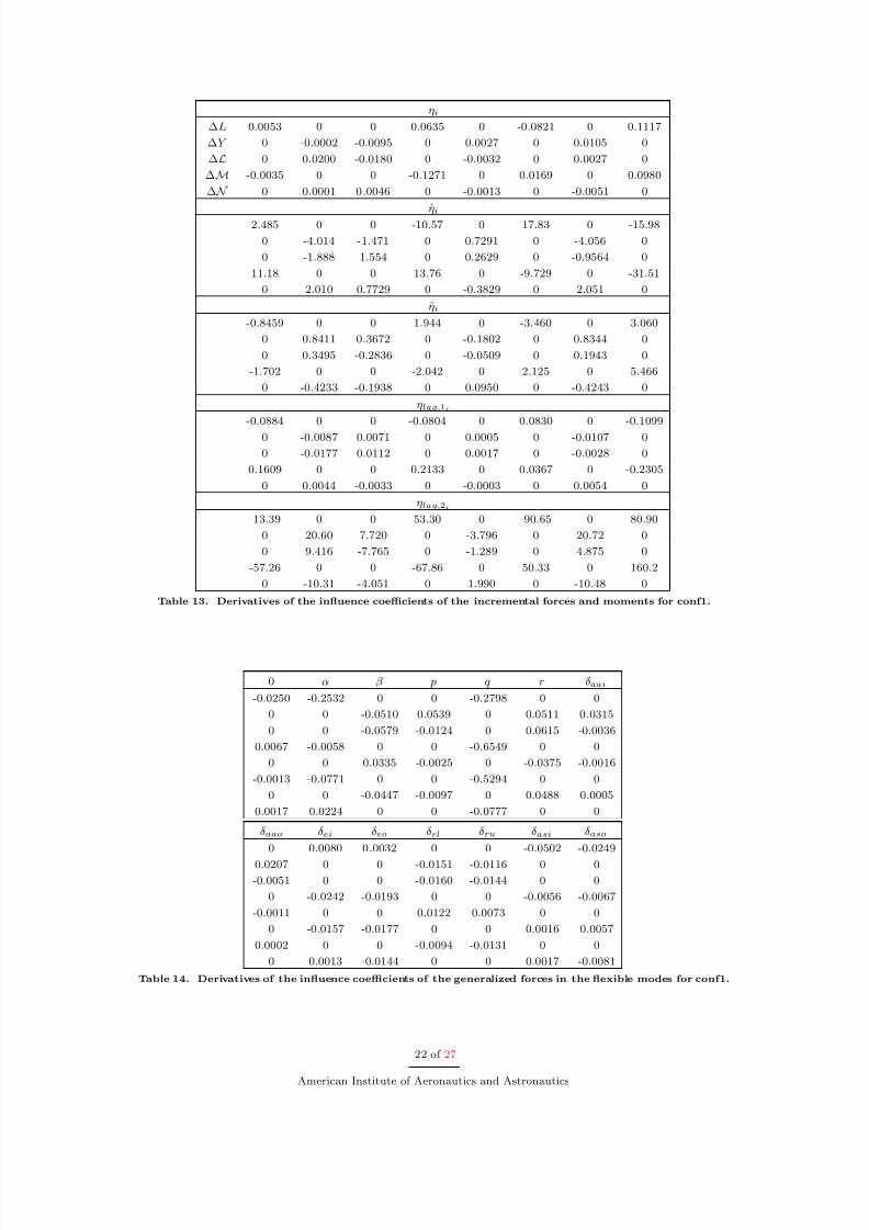
8/6/2019 daSilva2009


ηi

∆L 0.0053 0 0 0.0635 0 -0.0821 0 0.1117

∆Y 0 -0.0002 -0.0095 0 0.0027 0 0.0105 0

∆L 0 0.0200 -0.0180 0 -0.0032 0 0.0027 0

∆M -0.0035 0 0 -0.1271 0 0.0169 0 0.0980

∆ N 0 0.0001 0.0046 0 -0.0013 0 -0.0051 0

ηi

2.485 0 0 -10.57 0 17.83 0 -15.98

0 -4.014 -1.471 0 0.7291 0 -4.056 0

0 -1.888 1.554 0 0.2629 0 -0.9564 0

11.18 0 0 13.76 0 -9.729 0 -31.51

0 2.010 0.7729 0 -0.3829 0 2.051 0

ηi

-0.8459 0 0 1.944 0 -3.460 0 3.060

0 0.8411 0.3672 0 -0.1802 0 0.8344 0

0 0.3495 -0.2836 0 -0.0509 0 0.1943 0

-1.702 0 0 -2.042 0 2.125 0 5.466

0 -0.4233 -0.1938 0 0.0950 0 -0.4243 0

ηlag,1i

-0.0884 0 0 -0.0804 0 0.0830 0 -0.1099

0 -0.0087 0.0071 0 0.0005 0 -0.0107 0

0 -0.0177 0.0112 0 0.0017 0 -0.0028 0

0.1609 0 0 0.2133 0 0.0367 0 -0.2305

0 0.0044 -0.0033 0 -0.0003 0 0.0054 0

ηlag,2i

-13.39 0 0 53.30 0 -90.65 0 80.90

0 20.60 7.720 0 -3.796 0 20.72 0

0 9.416 -7.765 0 -1.289 0 4.875 0

-57.26 0 0 -67.86 0 50.33 0 160.2

0 -10.31 -4.051 0 1.990 0 -10.48 0

Table 13. Derivatives of the influence coefficients of the incremental forces and moments for conf1.

0 α β p q r δaai

-0.0250 -0.2532 0 0 -0.2798 0 0

0 0 -0.0510 0.0539 0 0.0511 0.0315

0 0 -0.0579 -0.0124 0 0.0615 -0.0036

0.0067 -0.0058 0 0 -0.6549 0 0

0 0 0.0335 -0.0025 0 -0.0375 -0.0016

-0.0013 -0.0771 0 0 -0.5294 0 0

0 0 -0.0447 -0.0097 0 0.0488 0.0005

0.0017 0.0224 0 0 -0.0777 0 0

δaao δei δeo δrl δru δasi δaso

0 0.0080 0.0032 0 0 -0.0502 -0.0249

0.0207 0 0 -0.0151 -0.0116 0 0-0.0051 0 0 -0.0160 -0.0144 0 0

0 -0.0242 -0.0193 0 0 -0.0056 -0.0067

-0.0011 0 0 0.0122 0.0073 0 0

0 -0.0157 -0.0177 0 0 0.0016 0.0057

0.0002 0 0 -0.0094 -0.0131 0 0

0 0.0013 -0.0144 0 0 0.0017 -0.0081

Table 14. Derivatives of the influence coefficients of the generalized forces in the flexible modes for conf1.

22 of 27


8/6/2019 daSilva2009


ηi

-0.0021 0 0 -0.0047 0 0.0093 0 -0.0201

0 -0.0049 0.0015 0 0.0001 0 0.0014 00 0.0002 -0.0016 0 -0.0002 0 0.0012 0

-0.0002 0 0 -0.0025 0 -0.0009 0 0.0017

0 -0.0003 -0.0003 0 -0.0011 0 0.0001 0

0.0003 0 0 -0.0015 0 -0.0008 0 0.0017

0 0.0001 -0.0007 0 0.0005 0 0.0006 0

0.0001 0 0 -0.0006 0 -0.0015 0 0.0009

ηi

-1.081 0 0 0.4805 0 -1.207 0 2.703

0 -0.8089 -0.3887 0 -0.0506 0 -0.4907 0

0 -0.5770 -0.2609 0 0.0250 0 -0.5082 0

0.2118 0 0 0.0883 0 0.0021 0 -0.8622

0 -0.1819 0.0739 0 -0.1999 0 0.1733 0

0.1353 0 0 0.1750 0 -0.2842 0 -0.2860

0 -0.2771 -0.1692 0 0.1247 0 -0.3895 0

0.1067 0 0 -0.1363 0 0.1175 0 -0.4931

ηi

0.2435 0 0 -0.0956 0 0.2273 0 -0.5151

0 0.1807 0.0855 0 0.0104 0 0.1010 0

0 0.1157 0.0665 0 -0.0059 0 0.1061 0

-0.0367 0 0 0.0012 0 0.0063 0 0.1641

0 0.0306 -0.0138 0 0.0494 0 -0.0400 0

-0.0254 0 0 -0.0233 0 0.0639 0 0.0552

0 0.0604 0.0410 0 -0.0303 0 0.0842 0

-0.0247 0 0 0.0362 0 -0.0203 0 0.1143

ηlag,1i

0.0022 0 0 0.0014 0 -0.0076 0 0.0160

0 -0.0003 -0.0002 0 -0.0001 0 -0.0014 0

0 -0.0018 0.0009 0 0.0001 0 -0.0013 0

0.0017 0 0 0.0036 0 0.0017 0 -0.0056

0 -0.0015 0.0002 0 0 0 0.0002 0

0.0015 0 0 0.0029 0 -0.0002 0 -0.0014

0 -0.0003 0.0005 0 0.0001 0 -0.0009 0

-0.0009 0 0 0.0005 0 0.0010 0 -0.0019

ηlag,2i

5.6941 0 0 -2.4219 0 6.0902 0 -13.6975

0 4.2750 1.9969 0 0.2804 0 2.5013 0

0 2.9611 1.3806 0 -0.1115 0 2.5956 0

-1.0809 0 0 -0.3803 0 0.0253 0 4.4212

0 0.9589 -0.3593 0 1.0766 0 -0.9028 0

-0.7102 0 0 -0.8526 0 1.4969 0 1.46940 1.4203 0.8816 0 -0.6576 0 2.0021 0

-0.5609 0 0 0.7367 0 -0.5709 0 2.5726


23 of 27


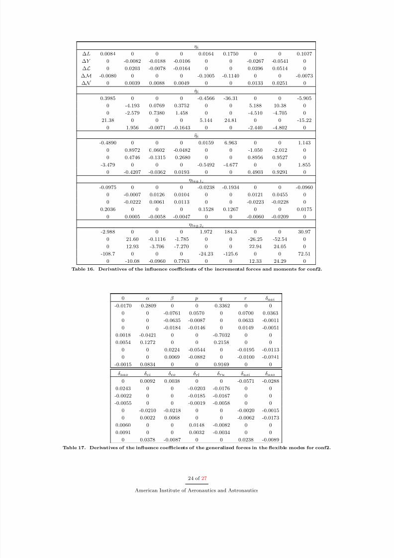
8/6/2019 daSilva2009


ηi

∆L 0.0084 0 0 0 0.0164 0.1750 0 0 0.1027

∆Y 0 -0.0082 -0.0188 -0.0106 0 0 -0.0267 -0.0541 0

∆L 0 0.0203 -0.0078 -0.0164 0 0 0.0396 0.0514 0

∆M -0.0080 0 0 0 -0.1005 -0.1140 0 0 -0.0073

∆ N 0 0.0039 0.0088 0.0049 0 0 0.0133 0.0251 0

ηi

0.3985 0 0 0 -0.4566 -36.31 0 0 -5.9050 -4.193 0.0769 0.3752 0 0 5.188 10.38 0

0 -2.579 0.7380 1.458 0 0 -4.510 -4.705 0

21.38 0 0 0 5.144 24.81 0 0 -15.22

0 1.956 -0.0071 -0.1643 0 0 -2.440 -4.802 0

ηi

-0.4890 0 0 0 0.0159 6.963 0 0 1.143

0 0.8972 0.0602 -0.0482 0 0 -1.050 -2.012 0

0 0.4746 -0.1315 -0.2680 0 0 0.8956 0.9527 0

-3.479 0 0 0 -0.5492 -4.677 0 0 1.855

0 -0.4207 -0.0362 0.0193 0 0 0.4903 0.9291 0

ηlag,1i

-0.0975 0 0 0 -0.0238 -0.1934 0 0 -0.0960

0 -0.0007 0.0126 0.0104 0 0 0.0121 0.0455 00 -0.0222 0.0061 0.0113 0 0 -0.0223 -0.0228 0

0.2036 0 0 0 0.1528 0.1267 0 0 0.0175

0 0.0005 -0.0058 -0.0047 0 0 -0.0060 -0.0209 0

ηlag,2i

-2.988 0 0 0 1.972 184.3 0 0 30.97

0 21.60 -0.1116 -1.785 0 0 -26.25 -52.54 0

0 12.93 -3.706 -7.270 0 0 22.94 24.05 0

-108.7 0 0 0 -24.23 -125.6 0 0 72.51

0 -10.08 -0.0960 0.7763 0 0 12.33 24.29 0


0 α β p q r δaai

-0.0170 -0.2809 0 0 -0.3362 0 0

0 0 -0.0761 0.0570 0 0.0700 0.0363

0 0 -0.0635 -0.0087 0 0.0633 -0.0011

0 0 -0.0184 -0.0146 0 0.0149 -0.0051

0.0018 -0.0421 0 0 -0.7032 0 0

0.0054 0.1272 0 0 0.2158 0 0

0 0 0.0224 -0.0544 0 -0.0195 -0.0113

0 0 0.0069 -0.0882 0 -0.0100 -0.0241

-0.0015 0.0834 0 0 0.9169 0 0


0 0.0092 0.0038 0 0 -0.0571 -0.0288

0.0243 0 0 -0.0203 -0.0176 0 0-0.0022 0 0 -0.0185 -0.0167 0 0

-0.0055 0 0 -0.0019 -0.0058 0 0

0 -0.0210 -0.0218 0 0 -0.0020 -0.0015

0 0.0022 0.0068 0 0 -0.0062 -0.0173

0.0060 0 0 0.0148 -0.0082 0 0

0.0091 0 0 0.0032 -0.0034 0 0

0 0.0378 -0.0087 0 0 0.0238 -0.0089


24 of 27


8/6/2019 daSilva2009


ηi

-0.0028 0 0 0 0.0004 -0.0233 0 0 -0.0375

0 -0.0079 -0.0009 -0.0008 0 0 -0.0193 -0.0340 0

0 -0.0002 -0.0027 -0.0001 0 0 -0.0022 -0.0025 0

0 -0.0007 -0.0001 -0.0031 0 0 -0.0016 -0.0012 0

0.0001 0 0 0 -0.0024 0.0004 0 0 -0.0013

-0.0007 0 0 0 0.0002 -0.0011 0 0 -0.0079

0 0.0018 -0.0004 -0.0012 0 0 0.0023 0.0036 0

0 0.0039 -0.0005 -0.0019 0 0 0.0068 0.0100 0

0.0011 0 0 0 0.0005 0.0080 0 0 0.0075

ηi

-1.489 0 0 0 -0.0928 2.776 0 0 4.295

0 -1.336 0.0513 -0.0964 0 0 2.182 3.805 0

0 -0.0607 -0.1395 0.0079 0 0 0.3573 0.8167 0

0 -0.7875 0.1362 -0.0250 0 0 0.3548 0.2261 0

0.2673 0 0 0 0.0209 0.3037 0 0 -0.0764

0.0219 0 0 0 0.0275 -1.018 0 0 0.2582

0 -0.1825 0.0089 0.1348 0 0 -0.8028 -1.0190 0

0 -0.1805 0.1016 0.2590 0 0 -1.403 -1.953 00.0590 0 0 0 -0.1652 -1.042 0 0 -1.480

ηi

0.3260 0 0 0 0.0142 -0.5317 0 0 -0.8380

0 0.2906 -0.0015 0.0295 0 0 -0.4220 -0.7479 0

0 0.0226 0.0404 -0.0029 0 0 -0.0690 -0.1527 0

0 0.1498 -0.0247 0.0198 0 0 -0.0673 -0.0522 0

-0.0487 0 0 0 0.0085 -0.0538 0 0 0.0186

-0.0032 0 0 0 -0.0072 0.2114 0 0 -0.0467

0 0.0390 0.0007 -0.0246 0 0 0.1735 0.2162 0

0 0.0358 -0.0201 -0.0506 0 0 0.2912 0.4100 0

-0.0351 0 0 0 0.0338 0.2197 0 0 0.3780

ηlag,1i

0.0030 0 0 0 -0.0016 0.0156 0 0 0.01910 0.0007 0.0017 0.0017 0 0 0.0084 0.0111 0

0 0.0012 0.0010 0.0002 0 0 0.0010 0.0064 0

0 -0.0027 0.0010 0.0020 0 0 0.0009 -0.0043 0

0.0016 0 0 0 0.0024 0.0018 0 0 0.0025

-0.0008 0 0 0 0 -0.0042 0 0 -0.0006

0 -0.0021 0.0002 0.0007 0 0 -0.0026 -0.0035 0

0 -0.0036 0.0003 0.0012 0 0 -0.0053 -0.0065 0

-0.0053 0 0 0 -0.0022 -0.0042 0 0 -0.0030

ηlag,2i

7.808 0 0 0 0.4632 -14.01 0 0 -21.78

0 7.029 -0.2589 0.5394 0 0 -11.01 -19.21 0

0 0.3004 0.7665 -0.0575 0 0 -1.799 -4.155 0

0 4.055 -0.7090 0.2129 0 0 -1.790 -1.110 0

-1.372 0 0 0 -0.0429 -1.556 0 0 0.3694

-0.0835 0 0 0 -0.1516 5.267 0 0 -1.238

0 0.9302 -0.0430 -0.6789 0 0 4.131 5.247 0

0 0.8835 -0.5222 -1.311 0 0 7.185 10.03 0

-0.3763 0 0 0 0.8592 5.303 0 0 7.780


25 of 27


8/6/2019 daSilva2009


ηi

∆L 0.0128 0 0 0.0243 0 0.1664 0 -0.1001 0

∆Y 0 -0.0152 -0.0254 0 0.0312 0 -0.0713 0 -0.1024

∆L 0 0.0181 -0.0034 0 0.0280 0 0.0508 0 -0.0042

∆M -0.0085 0 0 -0.1670 0 -0.1431 0 -0.4024 0

∆ N 0 0.0066 0.0109 0 -0.0134 0 0.0309 0 0.0451

ηi

0.5625 0 0 -0.8146 0 -35.11 0 10.25 00 -3.153 1.023 0 -1.863 0 14.96 0 19.42

0 -3.122 0.5105 0 -2.830 0 -5.590 0 2.389

25.47 0 0 10.68 0 32.39 0 185.8 0

0 1.376 -0.4004 0 0.7628 0 -6.362 0 -8.456

ηi

-0.5219 0 0 0.0734 0 6.764 0 -2.102 0

0 0.7106 -0.1145 0 0.2930 0 -2.918 0 -3.855

0 0.5744 -0.0891 0 0.5178 0 1.118 0 -0.4707

-4.196 0 0 -1.516 0 -6.027 0 -32.78 0

0 -0.3110 0.0392 0 -0.1160 0 1.239 0 1.674

ηlag,1i

-0.0942 0 0 -0.0304 0 -0.1793 0 0.0714 0

0 0.0104 0.0189 0 -0.0294 0 0.0631 0 0.06140 -0.0231 0.0041 0 -0.0225 0 -0.0260 0 0.0017

0.1973 0 0 0.2211 0 0.2027 0 1.625 0

0 -0.0042 -0.0080 0 0.0124 0 -0.0268 0 -0.0276

ηlag,2i

-4.046 0 0 3.697 0 178.2 0 -50.05 0

0 16.34 -4.864 0 9.157 0 -75.75 0 -98.29

0 15.69 -2.593 0 14.15 0 28.57 0 -12.22

-128.9 0 0 -51.75 0 -163.8 0 -947.9 0

0 -7.131 1.888 0 -3.738 0 32.20 0 42.78


0 α β p q r δaai

-0.0188 -0.3098 0 0 -0.4207 0 0

0 0 -0.0843 0.0520 0 0.0702 0.0370

0 0 -0.0726 -0.0059 0 0.0667 0.0004

0.0016 -0.0566 0 0 -0.8968 0 0

0 0 0.0559 0.0312 0 -0.0474 0.0091

0.0069 0.1428 0 0 0.1374 0 0

0 0 0.0287 -0.1040 0 -0.0246 -0.0293

0.0105 0.1768 0 0 0.5628 0 0

0 0 0.0697 0.0303 0 -0.0556 0.0084


0 0.0102 0.0045 0 0 -0.0645 -0.0334

0.0256 0 0 -0.0217 -0.0206 0 0-0.0006 0 0 -0.0211 -0.0194 0 0

0 -0.0231 -0.0267 0 0 -0.0019 -0.0011

0.0100 0 0 0.0113 0.0174 0 0

0 -0.0006 0.0031 0 0 -0.0052 -0.0203

0.0111 0 0 0.0138 -0.0062 0 0

0 0.0049 -0.0003 0 0 0.0433 -0.0065

-0.0010 0 0 0.0228 -0.0032 0 0


26 of 27


8/6/2019 daSilva2009


ηi

-0.0038 0 0 0.0013 0 -0.0267 0 -0.0212 0

0 -0.0101 -0.0009 0 0.0048 0 -0.0414 0 -0.0217

0 0 -0.0058 0 0 0 -0.0034 0 -0.0088

0.0002 0 0 -0.0040 0 0.0002 0 -0.0055 0

0 0.0026 0.0001 0 -0.0088 0 0.0065 0 0.0221

-0.0006 0 0 -0.0001 0 -0.0016 0 -0.0231 0

0 0.0046 0.0004 0 0.0026 0 0.0112 0 0.0061

0.0020 0 0 0 0 0.0136 0 0.0070 0

0 0 0.0016 0 -0.0033 0 0.0017 0 0.0053

ηi

-1.914 0 0 -0.1676 0 3.117 0 -0.3499 0

0 -1.590 0.2736 0 -0.3727 0 4.940 0 4.979

0 0.4695 -0.1564 0 0.1383 0 1.359 0 0.5516

0.2610 0 0 0.0844 0 0.6235 0 3.235 0

0 1.153 -0.2426 0 0.3337 0 -1.151 0 -4.600

0.1051 0 0 0.0479 0 -1.192 0 2.740 0

0 -0.2976 -0.0561 0 -0.3715 0 -3.110 0 -1.217

0.9733 0 0 0.0165 0 -2.238 0 -0.8164 00 0.3373 -0.1667 0 0.3643 0 -0.7690 0 -1.331

ηi

0.4144 0 0 0.0282 0 -0.6009 0 -0.0125 0

0 0.3407 -0.0448 0 0.0495 0 -0.9691 0 -0.9339

0 -0.0743 0.0510 0 -0.0246 0 -0.2508 0 -0.1415

-0.0486 0 0 -0.0017 0 -0.1090 0 -0.5601 0

0 -0.2261 0.0418 0 -0.0326 0 0.2323 0 0.8582

-0.0203 0 0 -0.0093 0 0.2510 0 -0.5039 0

0 0.0578 0.0109 0 0.0710 0 0.6451 0 0.2338

-0.2126 0 0 -0.0027 0 0.4510 0 0.2092 0

0 -0.0658 0.0315 0 -0.0724 0 0.1490 0 0.2703

ηlag,1i

0.0054 0 0 -0.0022 0 0.0170 0 -0.0232 00 0.0032 0.0024 0 -0.0064 0 0.0161 0 0.0303

0 0.0028 0.0025 0 0.0003 0 0.0105 0 -0.0071

0.0012 0 0 0.0035 0 0.0037 0 0.0305 0

0 0.0012 -0.0017 0 0.0072 0 0.0001 0 -0.0273

-0.0007 0 0 0.0005 0 -0.0036 0 0.0185 0

0 -0.0051 -0.0005 0 -0.0014 0 -0.0100 0 -0.0083

-0.0040 0 0 0 0 -0.0105 0 0.0055 0

0 0.0003 -0.0015 0 0.0034 0 -0.0030 0 -0.0038

ηlag,2i

10.00 0 0 0.8376 0 -15.73 0 1.750 0

0 8.340 -1.409 0 1.803 0 -24.93 0 -25.25

0 -2.408 0.9152 0 -0.6666 0 -6.912 0 -2.721

-1.342 0 0 -0.3433 0 -3.169 0 -16.49 0

0 -5.928 1.263 0 -1.531 0 5.785 0 23.32

-0.5055 0 0 -0.2479 0 6.183 0 -13.78 0

0 1.485 0.2752 0 1.886 0 15.96 0 6.155

-5.073 0 0 -0.0825 0 11.39 0 4.300 0

0 -1.725 0.8299 0 -1.832 0 3.884 0 6.768


Documents

daSilva2009