Embed Size (px)
Citation preview

Data Analysis Using R:5. Analysis of Variance
Tuan V. Nguyen
Garvan Institute of Medical Research,
Sydney, Australia

ANOVA and the concept of “Effect”
A B C
40-2 40+6 40-440-2 40+6 40-440-2 40+6 40-4
• There are differences between groups, but no differences within group.
• The model is now:– Yij = + j
• where = 40; 1 = -2, 2 = 6 and 3 = -4.
• Note that 1 + 2 + 3 = 0
A B C
38 46 3638 46 3638 46 36

ANOVA and the concept of “Effect”
A B C
40-2+5 40+6-5 40-4+340-2+2 40+6+1 40-4-240-2-3 40+6+8 40-4+1
A B C
43 41 3940 47 3435 54 37
39.3 47.3 36.7overall mean: 41.1
• In reality, there is always random variation in a population, so that there is sampling error.
• The model now includes an error term:Yij = + j + ij
• Effect of product A: 39.3-41.1 = -1.8product B: 47.3-41.1 = 5.8product C: 36.7-41.1 = -4.4

ANOVA Model
• Partition of variation into– Between groups– Within groups
• The model:
Yij = j ij
• Assumptions:
Normality
Independence
Homogeneity
• Var(Y) = Var() + Var() + Var()
= Var() + Var()

Variation between groupsA B C
43 41 3940 47 3435 54 37
Mean 39.3 47.3 36.7Overall mean: 41.1
The sum of squares for difference between groups:
(39.3 - 41.1)2 + (47.3 - 41.1)2 + (36.7 - 41.1)2 = 61.04
But the mean of each group is calculated from 3 observations. So the “true” sum of squares is:
SSb = 3*(39.3 - 41.1)2 + 3*(47.3 - 41.1)2 + 3*(36.7 - 41.1)2 = 184.8
Degrees of freedom: (3 groups – 1) = 2.

Variation within groupsA B C
43 41 3940 47 3435 54 37
Mean 39.3 47.3 36.7
SS for group A: SS1 = (43 – 39.3)2 + (40 – 39.3)2 + (35 – 39.3)2 = 32.7SS for group B: SS2 = (41 – 47.3)2 + (47 – 47.3)2 + (54 – 47.3)2 = 84.7SS for group C: SS3 = (39 – 36.7)2 + (34 – 36.7)2 + (37 – 36.7)2 = 12.7
SS for within group: SSW = SS1+SS2+SS3 = 130.0Degrees of freedom: (3 – 1) + (3 – 1) + (3 – 1) = 6

Summary of Analysis
Source of variation DF SS MS
Among groups 2 184.8 92.4
Within groups 6 130.0 21.7
Total 8 314.8
• F statistic = MSa / MSw = 92.4 / 21.7 = 4.27• P value associated with (2, 6) df: 0.07

ANOVA by R
group <- c(1,1,1,2,2,2,3,3,3)
y <- c(43, 40, 35, 41, 47, 54, 39, 34, 37)
group <- as.factor(group)
analysis <- lm(y ~ group)
summary(analysis)
anova(analysis)
A B C
43 41 3940 47 3435 54 37

Summary of Variation
> anova(analysis)Response: y
Df Sum Sq Mean Sq F value Pr(>F)
group 2 184.889 92.444 4.2667 0.07037 .
Residuals 6 130.000 21.667
---
Signif. codes: 0 '***' 0.001 '**' 0.01 '*' 0.05 '.' 0.1 ' ' 1

Estimate of Treatment Effects> summary(analysis)...
Coefficients:
Estimate Std. Error t value Pr(>|t|)
(Intercept) 39.333 2.687 14.636 6.39e-06 ***
group2 8.000 3.801 2.105 0.080 .
group3 -2.667 3.801 -0.702 0.509
---
Signif. codes: 0 '***' 0.001 '**' 0.01 '*' 0.05 '.' 0.1 ' ' 1
Residual standard error: 4.655 on 6 degrees of freedom
Multiple R-Squared: 0.5872, Adjusted R-squared: 0.4495
F-statistic: 4.267 on 2 and 6 DF, p-value: 0.07037

Multiple Comparisons: Tukey’s Method
res <- aov(y ~ group)TukeyHSD (res)
Tukey multiple comparisons of means 95% family-wise confidence level
Fit: aov(formula = y ~ group)
$group diff lwr upr p adj2-1 8.000000 -3.661237 19.6612370 0.16894003-1 -2.666667 -14.327904 8.9945703 0.77141793-2 -10.666667 -22.327904 0.9945703 0.0692401

Multiple Comparisons: Tukey’s Method
plot(TukeyHSD(res), ordered=T)
-20 -10 0 10 20
3-2
3-1
2-1
95% family-wise confidence level
Differences in mean levels of group

Graphical Analysisaverage <- tapply(y, group, mean)
std <- tapply(y, group, sd)
ss <- tapply(y, group, length)
sem <- std/sqrt(ss)
stripchart(y ~ group, "jitter", jit=0.05, pch=16, vert=TRUE)
arrows(1:3, average+sem, 1:3, average-sem, angle=90, code=3, length=0.1)
lines(1:3, average, pch=4, type="b", cex=2)

Graphical Analysis
1 2 3
35
40
45
50

Factorial ANOVA
Variety Pesticide Total
1 2 3 4
B1 29 50 43 53 175
B2 41 58 42 73 214
B3 66 85 63 85 305
Tổng số
136 193 154 211 694
Model:
product = a + b(variety) + g(pesticide) + e

Factorial ANOVA by RVariety Pesticide Total
1 2 3 4
B1 29 50 43 53 175
B2 41 58 42 73 214
B3 66 85 63 85 305
Tổng số 136 193 154 211 694
variety <- c(1, 1, 1, 1, 2, 2, 2, 2, 3, 3, 3, 3)pesticide <- c(1, 2, 3, 4, 1, 2, 3, 4, 1, 2, 3, 4)product <- c(29,50,43,53,41,58,42,73,66,85,69,85)
variety <- as.factor(variety) pesticide <- as.factor(pesticide) data <- data.frame(variety, pesticide, product)

Factorial ANOVA by Ranalysis <- aov(product ~ variety + pesticide)anova(analysis)
Analysis of Variance TableResponse: product Df Sum Sq Mean Sq F value Pr(>F) variety 2 2225.17 1112.58 44.063 0.000259 ***pesticide 3 1191.00 397.00 15.723 0.003008 ** Residuals 6 151.50 25.25 ---Signif. codes: 0 '***' 0.001 '**' 0.01 '*' 0.05 '.' 0.1 ' ' 1

Multiple Comparisons
> TukeyHSD(analysis)
Tukey multiple comparisons of means 95% family-wise confidence levelFit: aov(formula = product ~ variety + pesticide)$variety diff lwr upr p adj2-1 9.75 -1.152093 20.65209 0.07491033-1 32.50 21.597907 43.40209 0.00023633-2 22.75 11.847907 33.65209 0.0016627
$pesticide diff lwr upr p adj2-1 19 4.797136 33.202864 0.01405093-1 6 -8.202864 20.202864 0.51061524-1 25 10.797136 39.202864 0.00361093-2 -13 -27.202864 1.202864 0.07042334-2 6 -8.202864 20.202864 0.51061524-3 19 4.797136 33.202864 0.0140509
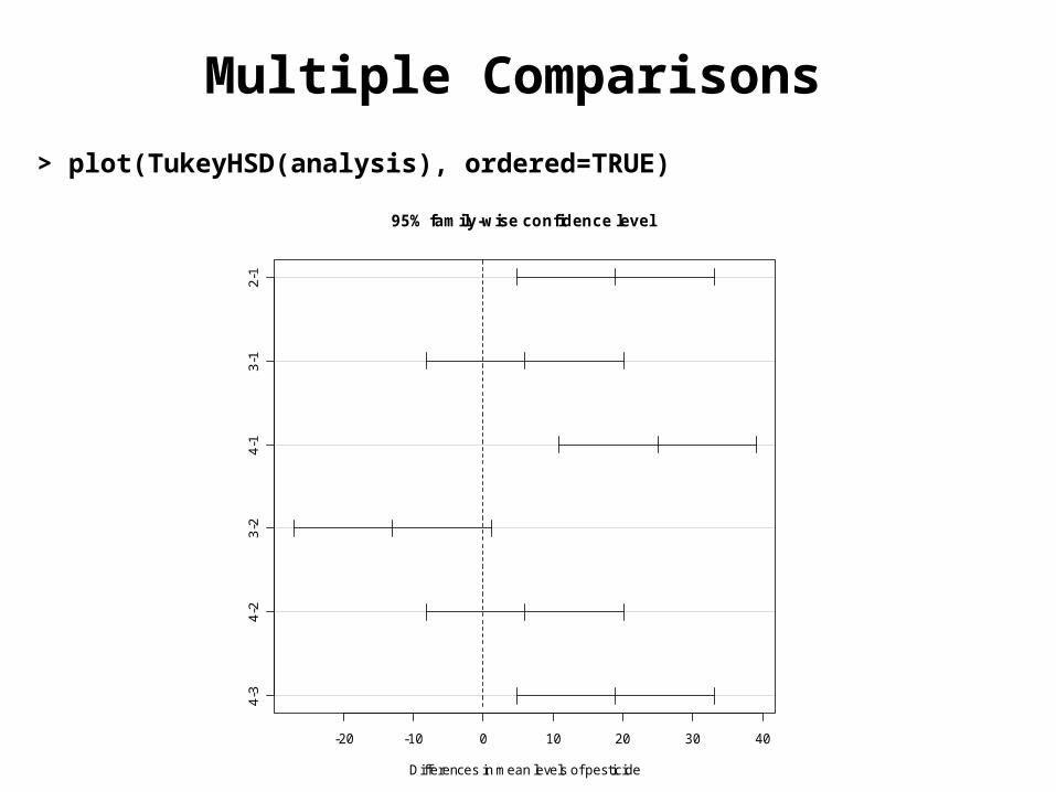
Multiple Comparisons
> plot(TukeyHSD(analysis), ordered=TRUE)
-20 -10 0 10 20 30 40
4-3
4-2
3-2
4-1
3-1
2-1
95% family-wise confidence level
Differences in mean levels of pesticide

Latin-square ANOVA
Plot Variety
1 2 3 4
1 175Aa
143Ba
128Bb
166Ab
2 170Ab
178Aa
140Ba
131Bb
3 135Bb
173Ab
169Aa
141Ba
4 145Ba
136Bb
165Ab
173Aa

Latin-square ANOVA: summary
Plot Variety
1 2 3 4
1 175Aa
143Ba
128Bb
166Ab
2 170Ab
178Aa
140Ba
131Bb
3 135Bb
173Ab
169Aa
141Ba
4 145Ba
136Bb
165Ab
173Aa
Mean by variety Mean by plot Mean by method
1: 156.252: 157.503: 150.504: 152.75Overall mean: 154.25
1: 153.002: 154.753: 154.504: 154.75Overall mean: 154.25
1 (Aa): 173.752 (Ab): 168.503 (Ba): 142.254 (Bb): 132.50Overall mean: 154.25

Latin-square ANOVA by RPlot Variety
1 2 3 4
1 175Aa
143Ba
128Bb
166Ab
2 170Ab
178Aa
140Ba
131Bb
3 135Bb
173Ab
169Aa
141Ba
4 145Ba
136Bb
165Ab
173Aa
y <- c(175, 143, 128, 166, 170, 178, 140, 131, 135, 173, 169, 141, 145, 136, 165, 173)
variety <- c(1,2,3,4, 1,2,3,4, 1,2,3,4, 1,2,3,4,) sample <- c(1,1,1,1, 2,2,2,2, 3,3,3,3, 4,4,4,4) method <- c(1, 3, 4, 2, 2, 1, 3, 4, 4, 2, 1, 3, 3, 4, 2, 1)
variety <- as.factor(variety)sample <- as.factor(sample)method <- as.factor(method)

Latin-square ANOVA by R
latin <- aov(y ~ sample + variety + method)summary(latin)
Df Sum Sq Mean Sq F value Pr(>F) sample 3 8.5 2.8 2.2667 0.1810039 variety 3 123.5 41.2 32.9333 0.0004016 ***method 3 4801.5 1600.5 1280.4000 8.293e-09 ***Residuals 6 7.5 1.3 ---Signif. codes: 0 '***' 0.001 '**' 0.01 '*' 0.05 '.'
0.1 ' ' 1

Latin-square – Multiple Comparisons
> TukeyHSD(latin)$variety diff lwr upr p adj2-1 1.25 -1.4867231 3.9867231 0.45285493-1 -5.75 -8.4867231 -3.0132769 0.00141524-1 -3.50 -6.2367231 -0.7632769 0.01732063-2 -7.00 -9.7367231 -4.2632769 0.00048034-2 -4.75 -7.4867231 -2.0132769 0.00388274-3 2.25 -0.4867231 4.9867231 0.1034761
$method diff lwr upr p adj2-1 -5.25 -7.986723 -2.513277 0.00230163-1 -31.50 -34.236723 -28.763277 0.00000014-1 -41.25 -43.986723 -38.513277 0.00000003-2 -26.25 -28.986723 -23.513277 0.00000044-2 -36.00 -38.736723 -33.263277 0.00000004-3 -9.75 -12.486723 -7.013277 0.0000730

Graphical Analysis
boxplot(y ~ method, xlab="Methods (1=Aa, 2=Ab, 3=Ba, 4=Bb", ylab="Production")
1 2 3 4
13
01
40
15
01
60
17
01
80
Methods (1=Aa, 2=Ab, 3=Ba, 4=Bb
Pro
du
ctio
n

Cross-over Study ANOVANhóm Mã số bệnh nhân số
(id)Thời gian (phút) ra mồ hôi trên trán
Tháng 1 Tháng 2
AB A Placebo
1 6 4
3 8 7
5 12 6
6 7 8
9 9 10
10 6 4
13 11 6
15 8 8
BA Placebo A
2 5 7
4 9 6
7 7 11
8 4 7
11 9 8
12 5 4
14 8 9
16 9 13

Cross-over Study ANOVA by R
y <- c(6,8,12,7,9,6,11,8, 4,7,6,8,10,4,6,8, 5,9,7,4,9,5,8,9 7,6,11,7,8,4,9,13)seq <- c(1,1,1,1,1,1,1,1, 1,1,1,1,1,1,1,1, 2,2,2,2,2,2,2,2, 2,2,2,2,2,2,2,2)period <- c(1,1,1,1,1,1,1,1, 2,2,2,2,2,2,2,2, 2,2,2,2,2,2,2,2, 1,1,1,1,1,1,1,1)treat <- c(1,1,1,1,1,1,1,1, 2,2,2,2,2,2,2,2, 1,1,1,1,1,1,1,1, 2,2,2,2,2,2,2,2)id <- c(1,3,5,6,9,10,13,15, 1,3,5,6,9,10,13,15, 2,4,7,8,11,12,14,16,
2,4,7,8,11,12,14,16)
seq <- as.factor(seq) period <- as.factor(period) treat <- as.factor(treat) id <- as.factor(id)
data <- data.frame(seq, period, treat, id, y)

Cross-over Study ANOVA by R
xover <- lm(y ~ treat + seq + period)anova(xover)
Analysis of Variance TableResponse: y Df Sum Sq Mean Sq F value Pr(>F) treat 1 16.531 16.531 4.9046 0.04388 *seq 1 0.031 0.031 0.0093 0.92466 period 1 0.781 0.781 0.2318 0.63764 id 14 103.438 7.388 2.1921 0.07711 .Residuals 14 47.187 3.371 ---Signif. codes: 0 '***' 0.001 '**' 0.01 '*' 0.05 '.' 0.1 ' ' 1

Cross-over Study ANOVA by R
> TukeyHSD(aov(y ~ treat+seq+period+id))
Tukey multiple comparisons of means 95% family-wise confidence levelFit: aov(formula = y ~ treat + seq + period + id)
$treat diff lwr upr p adj2-1 -1.4375 -2.829658 -0.04534186 0.0438783
$seq diff lwr upr p adj2-1 0.0625 -1.329658 1.454658 0.924656
$period diff lwr upr p adj2-1 -0.3125 -1.704658 1.079658 0.6376395