Embed Size (px)
Citation preview

i
The Islamic University Gaza
Higher Education Deanship
Faculty of Engineering
Electrical Engineering
غزة – اإلسالميت الجامعت
العليا الذراساث عمادة
الهنذست كليت
الهنذست الكهربائيت
باستخذام ترميز التيربى والمخارج المذاخل متعذدة االتصاالثطرق الكشف ألوظمت
Detection Methods for MIMO System Using Turbo Code
Submitted by:
Eng. Alaa AL Habbash
Supervised by:
Dr. Ammar M. Abu Hudrouss
This Thesis is Submitted in Partial Fulfillment of the Requirements for the
Degree of Master of Science in Electrical Engineering
م -2013هـ 1434

ii
Detection Methods for MIMO System Using Turbo Codes
By:
Alaa H. M. Al Habbash
Supervisor:
Dr. Ammar M. Abu Hudrouss
ABSTRACT
Multiple-Input-Multiple-Output (MIMO) communication techniques have been an important
area of focus for 4th
generation wireless systems. This is mainly because of their potentials for
high capacity, increased diversity, and interference suppression. There are many schemes that
can be applied to MIMO systems such as Space-Time Block Codes (STBCs), Space-Time Trellis
Codes (STTCs), and the Vertical Bell Labs Space-Time Architecture (V-BLAST). STBC and
STTCs are used for diversity gain while VBLAST is used for capacity advantage.
There are many types of detection techniques were introduced for spatial multiplexing
MIMO channels. Vertical Bell Labs Space-Time Architecture/ Maximum A-Posteriori (V-
BLAST/MAP) is a new symbol detection algorithm for MIMO channels, which is an extension
of the well-known V-BLAST algorithm. Another algorithm which is a V-BLAST/MAP,
algorithm combines elements of the V-BLAST algorithm and the maximum a-posteriori (MAP)
rule. The performance improvement is significant. Simulations show that V-BLAST/MAP
achieves symbol error rates close to the optimal maximum likelihood (ML) scheme while
retaining the low-complexity nature of the V-BLAST.
In the nineties, a novel method of coding that has become known as Turbo Coding was
developed. Turbo coding introduced to prevent or reduce the effects of burst error by using
several convolutional coders and a random interleaver. Turbo Coding has proved to be the most

iii
efficient code developed so far, capable of operating close to the Shannon limit with a reasonable
complexity.
Recently, some of high potential research considers the case of using principle of iterative
(„Turbo processing‟) in improving the performance of multiple antenna systems. One of the
resulting classes of MIMO system referred to as Turbo-V-BLAST. Therefore, Turbo codes with
independent fading coefficients at each coded bit in a codeword will get the best performance.
In this research, the performance of Turbo-V-BLAST algorithm with different types of
detection is evaluated. First, the V-BLAST algorithm with zero forcing (ZF), Linear Least
Square Estimation (LLSE) and MAP detections is reviewed and the error rate of this algorithm is
investigated. Next, the V-BLAST algorithm is combined with Turbo code and the performance
of Turbo-V-BLAST algorithm with ZF, LLSE and MAP detections was evaluated. Then, the
novel approach of using MAP detection technique with Turbo-V-BLAST is introduced . The
performance of the new algorithm is derived.

iv
باستخذام ترميز والمخارج المذاخل متعذدة االتصاالثطرق الكشف ألوظمت
التيربى
عالء حسيه محمذ الهباش : إعذاد
دروسھ أبى محمذ رمضان محمذ عمار .د : المشرف
الملخص
من بعاالر الجيل في اهلتطبيق والبحث تمامهلال المثيرة التقنيات أكثر من ( MIMO ) والمخارج المداخل متعددة االتصاالت تقنيات تعتبر إخماد ىلع اهوقدرت (Channel Capacity) االتصال لقناة السعة زيادة في الكبير اهدور بسبب وذلك ,كيةلالالس االتصاالت أنظمة
الترميزمثل (MIMO) هناك العديد من الخطط التي يمكن تطبيقها على أنظمة .النظام في الخطأ معدل يللتق وأيضا والتشويش التداخل (Space Time Trellis Coding STTC) الشبكي الزمكاني الترميزو ((Space Time Block Coding-STBC يلالكت الزمكاني
(.Vertical Bell Labs Space-Time Architecture- V-BLAST)العمودية ، و أنظمة البالست
ومنها األنظمة البالست مع تقنية . والمخارج المداخل متعددة االتصاالت تقنياتهناك العديد من تقنيات اكتشاف الرموز المقترحة لقنوات و هي (Vertical Bell Labs Space-Time / Maximum A-Posteriori -V-BLAST/MAP) الحد األقصى البعدية لمكشف
و تجمع بين خصائص انظمة البالست العمودية و خصائص , تقنية جديدة لمكشف وتعتبر امتداد ألنظمة البالست العمودية المعروفةوتعمل عمى , وتختمف عن أنظمة البالست العمودية العادية في االستراتيجية ترتيب الرموز المكتشفة فقط, تقنية الحد األقصى البعدية
بالمقارنة مع أنظمة ”(Maximum Likelihood -ML) قريب من تقنية احتمال الحد األقصى األمثل ”تحسين األداء بشكل ممحوظ . البالست العادية مع االحتفاظ بخاصية قمة التعقيد الموجود بأنظمة البالست العمودية
يمنع أو يحد ترميز التيربو . (Turbo coding)في بداية التسعينات، ظهرت طريقة جديدة لمترميز والتي أصبحت تعرف باسم ترميز التيربو
ويعتبر ترميز التيربو من أكثر المرمزات فعالية حتى . حدوث األخطاء باستخدام عدة مشفرات تالفيفية باإلضافة إلى مرتب مشذر عشوائيو مؤخرا، أجريت بعض البحوث الستخدام مبدأ . اآلن، حيث إنها قادرة عمى العمل بكفاءة عمى مقربة من حد شانون مع نسبة تعقيد مقبولة
Turbo -Vertical Bell)في تحسين أداء األنظمة متعددة الهوائيات حيث ظهرت تقنية تيربو بالست العمودية ('توربو معالجة')التكرار Labs Space-Time- Turbo-V-BLAST) الخي جمعج حرميز الخيربى وانظمت البالسج العمىديت للخروج بكفاءة أفضل من كل منها
.على حذة
أوال، يتم مراجعة أنظمة البالست مع الكشف بطريقة . في هذا البحث، فإننا نقيم أداء تيربو بالست العمودية مع أنواع مختمفة من الكشف LLSE- (Linear Least Square Estimation )، وطريقة الحد األدنى لمتوسط تربيع الخطأZero Forcing-ZF) (التصفير بالقوة

v
وبعد ذلك، يتم الجمع بين أنظمة البالست مع ترميز التيربو لتقييم . وطريقة الحد األقصى البعدية والتحقيق في معدل خطأ نقل البياناتوطريقة الحد التصفير بالقوة وطريقة الحد األدنى لمتوسط تربيع الخطأ: اداء تقنية تيربو بالست العمودية مع طرق الكشف التالية
ومن ثم التحقق من مدى كفاءة استخدام تقنية تقنية تيربو بالست العمودية مع الكشف باستخدام طريقة الحد األقصى , األقصى البعدية .البعدية

vi
DEDICATIONS
All praises goes to Allah, the Creator of all things in the world
To my parents Who encouraged me and have given me endless support during the work of this thesis.
To my beloved Aunt and Uncle, Saeed and Fatimah
Who taught me the value of study and Spirit of perseverance
To my dear wife and brothers For their patience and their continued support
To my children Mohammed and Mona
For their preeminence face
To my great family
To my special friends
To my beloved country
To all whom I love

vii
ACKNOWLEDGEMENTS
First of all, without the enlightenment of ALLAH, this work would not have been done
successfully.
My sincere appreciation goes to Dr. Ammar M. Abu-Hudrouss for his valuable guidance
and encouragement. I have benefited tremendously from his enthusiasm, understanding, and
patience. I also hereby offer my special gratitude to Dr. Fadi Alnahal and Dr. Yousef Hammoda
my examiners and teachers.
I would like to thank my colleagues in the MTIT, especially Eng. Abd El Ghani E. Abu
Tair, for their moral support. Thanks also go to my dear friends, Mohammed Taha El Astal and
Mohammed El Awaity for their help, friendship, and all the wonderful time we share.
Last, I would mostly like to thank my parents for their love and prayers through my life.
Special thanks to my wife for her support, patience and prayers which accompanied me all the
way along. Also I would like to thank my brothers for their love, trust and responsibility. And
thanks to my dear sisters and all my precious family.
Alaa H. Al Habbash
April, 2013

viii
TABLE OF CONTENTS ABSTRACT ........................................................................................................................................... ii
DEDICATIONS ................................................................................................................................... vi
ACKNOWLEDGEMENTS ................................................................................................................ vii
TABLE OF CONTENTS .................................................................................................................. viii
LIST OF FIGURES .............................................................................................................................. xi
LIST OF ABBREVIATIONS ............................................................................................................. xiv
Chapter 1: Introduction .......................................................................................................................... 1
1.1 Introduction ........................................................................................................................................ 1
1.2 Motivation .......................................................................................................................................... 2
1.3 Problem statement .............................................................................................................................. 2
1.4 Literature Review ............................................................................................................................... 3
1.5 Objectives ........................................................................................................................................... 4
1.6 Thesis Contributions ........................................................................................................................... 4
1.7 Thesis Organization ............................................................................................................................ 5
Reference .................................................................................................................................................. 7
Chapter 2: MIMO Communication Systems ......................................................................................... 9
2.1 Introduction ........................................................................................................................................ 9
2.2 Shannon‟s Capacity Theorem ........................................................................................................... 10
2.3 The MIMO Channel Model .............................................................................................................. 10
2.4 The Symbols Detection Problem ...................................................................................................... 12
2.5 Detection Algorithms........................................................................................................................ 15
2.6 Linear Receivers ............................................................................................................................... 16
2.6.1 Zero-Forcing (ZF) Receiver ................................................................................................ 16
2.6.2 Linear Least Square Estimation (LLSE) Receiver .............................................................. 17
2.7 V-BLAST System ............................................................................................................................. 18
2.7.1 V-BLAST Architecture ....................................................................................................... 19
2.8 V-BLAST/MAP Detection Algorithm .............................................................................................. 25
2.8.1 V-BLAST/ZF/MAP Detection Algorithm ...................................................................................... 26
2.8.2 V-BLAST/LLSE/MAP Detection Algorithm ............................................................................ 29
References ............................................................................................................................................... 31
Chapter 3: Turbo Codes ....................................................................................................................... 33
3.1 Introduction ....................................................................................................................................... 33

ix
3.2 Channel codes: .................................................................................................................................. 34
3.2.1 Block Codes ................................................................................................................................ 34
3.2.2 Convolutional Code .................................................................................................................... 34
3.2.3 Turbo Codes ............................................................................................................................... 35
3.3 Convolutional Codes ......................................................................................................................... 36
3.3.1 Encoder Structure ....................................................................................................................... 36
3.3.2 Equivalent Encoders .................................................................................................................. 37
3.3.3 Convolutional Codes Decoding ................................................................................................. 38
3.3.4 Free Distance ............................................................................................................................. 40
3.4 Turbo Code Encoding ....................................................................................................................... 41
3.4.1 Classification of Concatenated Codes ........................................................................................ 41
3.4.2 Encoding Operation ................................................................................................................... 42
3.5 Spectral Thinning and Random Interleavers ..................................................................................... 46
3.6 Punctured Turbo Codes ..................................................................................................................... 48
3.7 SOVA/log-MAP Turbo Decoder ...................................................................................................... 49
3.7.1 Structure of Iterative Decoding .................................................................................................. 50
3.7.2 Decoding Algorithms ................................................................................................................. 52
3.8 Conclusion ........................................................................................................................................ 58
References ............................................................................................................................................... 59
Chapter 4: Uncoded and Turbo Coded V-BLAST Architectures ........................................................ 62
4.1 Introduction ....................................................................................................................................... 62
4.2 Uncoded V-BLAST System.............................................................................................................. 63
4.2.1 Uncoded V-BLAST Transmitter ................................................................................................ 63
4.2.2 Uncoded V-BLAST Receiver .................................................................................................... 65
4.3 Coded V-BLAST MIMO System ..................................................................................................... 66
4.3.1 Coded V-BLAST MIMO Transmitter ....................................................................................... 66
4.3.2 Coded V-BLAST MIMO Receiver ............................................................................................ 67
4.4 Simulation Results ............................................................................................................................ 70
4.4.1 Performance Analysis .............................................................................................................. 71
4.5 Conclusion ........................................................................................................................................ 79
References ............................................................................................................................................... 80
Chapter 5: Conclusions ......................................................................................................................... 81

x
5.1 Conclusion ..................................................................................................................................... 81
5.2 Future works: ................................................................................................................................. 82

xi
LIST OF FIGURES
Figure 2.1: Multiple Input Multiple Output (MIMO) channel model…………………………………….12
Figure 2.2: Modulation, transmission and decision in MIMO wireless systems…………………………13
Figure 2.3: SER of ZF, LLSE, VBLAST-ZF, and VBLAST-LLSE receivers without coding………….17
Figure 2.4: Block diagram of V-BLAST architecture…………………………………………………….20
Figure 2.5: Different V-BLAST Algorithms……………………………………………………………...22
Figure 2.6: V-BLAST/ZF Detection Algorithm…………………………………………………………..24
Figure 2.7: V-BLAST/LLSE Detection Algorithm…………………………………………………….....25
Figure 2.8: Symbol error rates (SER) of V-BLAST/ZF/MAP receiver-BLAST/ZF receiver and ML
receiver. The simulation is for (M, N) = (4, 12) and 4-QAM modulation...................................................26
Figure 2.9: V-BLAST/ZF/MAP Detection Algorithm................................................................................27
Figure 2.10: V-BLAST/ZF/MAP Detection Algorithm…………………………………………………........29
Figure 2.11: Symbol error rate (SER) of VBLAST/ZF/MAP receiver, VBLAST/LLSE/MAP receiver,
VBLAST/ZF receiver and VBLAST/LLSE receiver………………………………………………..........29
Figure 3.1: The parallel-concatenated convolution codes by a rate of 1/3.…………………....................35
Figure 3.2: Rate-1/2 feedforward convolutional encoder with two memory elements (four states)……...36
Figure 3.3: Rate-1/2 feedback convolutional encoder with two memory elements (four states)………...37
Figure 3.4: State diagram for rate-1/2 feedforward convolutional encoder of Fig. 3.2…………………..37
Figure 3.5: State diagram for rate-1/2 feedback convolutional encoder of Fig. 3.3………………….......38
Figure 3.6: One stage of the trellis diagram for rate-1/2 feedforward convolutional encoder of Figs. 3.2
and 3.3..........................................................................................................................................................39
Figure 3.7: Free Hamming distance of the code described by Figs. 3.2, 3.4, and 3.6.................................41
Figure 3.8: Encoder structures for (a) PCCCs and (b) SCCCs …...............................................................42
Figure 3.9: A constraint-length 3, RSC encoder with generator matrix octal
G = 7,5 ..................................43

xii
Figure 3.10: Bit error rate of Turbo code with frame size = 1000, iteration=4, number of frames = 100,
puncture, and by using log-map decoding……………………………………………………………….. 44
Figure 3.11: Bit error rate of Turbo code with frame size = 1000, iteration=4, number of frames = 100,
un-puncture, and by using log-map decoding……………………………………………...……………...45
Figure 3.12: Recursive convolutional encoder with three delay states and overall rate…………………..47
Figure 3.13: Efficiency difference between log-MAP and SOVA (4-iteration, puncture and frame
size=1000)………………………………………………………………………………………………....50
Figure 3.14: Conventional Turbo decoder …...………………………...……………..…………………..51
Figure 3.15: Trellis-based decoding algorithms…...………………...……………………………………53
Figure.4.1: Uncoded V-BLAST Transmitter………...……………………………………………………64
Figure 4.2: Uncoded V-BLAST Vectors at Transmitter…………………...……………………………...64
Figure 4.3: Uncoded V-BLAST Receiver………………………………………………………………....65
Figure 4.4: coded V-BLAST Transmitter…………………………………………………………….…...68
Figure 4.5: Codewords interleaving at the transmitter…………………………………………………….68
Figure 4.6: coded V-BLAST Receiver……………………………………………………………………69
Figure 4.7: Illustration of how the generator polynomials determined…………………………………....71
Figure 4.8: The SER performance for different frame size of Turbo/ normal LLSE……………………..72
Figure 4.9: The SER performance for coded V-BLAST/ZF using Turbo code and coded V-BLAST/ZF
using Turbo code with best order………………………………………………...………………………..74
Figure 4.10: The SER performance for coded V-BLAST/LLSE using Turbo code and coded V-
BLAST/LLSE using Turbo code with best order………………………………..………………...……...74
Figure 4.11: The SER performance for coded normal ZF, V-BLAST/ZF and V-BLAST/ZF/MAP using
Turbo……………………………………………………...……………………………………………….75
Figure 4.12: SER performance for coded normal LLSE, V-BLAST/LLSE and V-BLAST/LLSE/MAP
using Turbo………………………………………………………..………………………………………76
Figure 4.13: SER performance for uncoded V-BLAST/ZF and coded V-BLAST/ZF using Turbo code...77
Figure 4.14: SER performance for uncoded V-BLAST/LLSE and coded V-BLAST/LLSE using Turbo
code………………………………………………………………………………………………………..78
Figure 4.15: SER performance for coded V-BLAST/LLSE using Turbo code with two
iterations…………………………………………………………………………………………………...78

xiii
LIST OF TABLES
Table 4.1. The parameters of a 1/2 rate convolution code. .................................................................. 71
Table 4.2: Puncturing patterns ............................................................................................................. 71

xiv
LIST OF ABBREVIATIONS
BER Bit Error Rate
SER Symbol Error Rate
MIMO Multiple Input- Multiple Output
V-BLAST Vertical Bell Labs Layered Space-Time
D-BLAST Diagonal Bell Labs Layered Space-Time
LLSE Linear Least Square Estimation
ZF Zero-Forcing
ML Maximum Likelihood
MAP Maximum A-Posteriori
LDPC Low-density Parity-check codes
BCH Bose, Ray-Chaudhuri, and Hocquengham.
PCCC Parallel Concatenated Convolution Code
SCCC Serial Concatenated Convolution Code
HCCC Hybrid Concatenated Convolution Code
RSC Recursive and Systematic Convolutional
AWGN Additive White Gaussian Noise
SNR Signal to Noise Ratio
CSI Channel State Information
QAM Quadrature Amplitude Modulation
BPSK Binary Phase Shift Keying
Pe Probability of Decision Error
APP A posteriori probabilities
SOVA Soft Output Viterbi Algorithm
LOG-MAP Log Maximum A Posteriori Algorithm
SISO Soft Input-Soft Output

xv
VA Viterbe Algorithm
LLR Log-Likelihood Ratio
BCJR Bahl, Cocke, Jelinek and Raviv Algorithm
i.i.d Independent and Identically Distributed
Eb Average Bit Energy

1
Chapter 1
Introduction
1.1 Introduction:
The paper of Claude Shannon, which published in 1949, demonstrated the mathematical
basis of the maximum capacity of a noisy communications channel [1]. Subsequently, this limit
is known as “Shannon limit” of the channel capacity. He stated that an error correcting code
exists to achieve this limit. Since that time, many research efforts have tried to design such code
to approach the Shannon capacity[6]. Although there is a good progress in this problem but all
designed codes have assumed an availability of large block length to have a capacity close to the
Shannon capacity[6]. The requirement make these codes impractical for some applications as it
impose many consequences such as; complexity, cost and latency.
Turbo codes, a new class of convolution codes, proposed in 1993 [2]. It gets a 0.7 dB of
the Shannon limit in terms of Bit Error Rates (BER). It has a high potential for both of academic
and industrial researchers [2]. Recently, some of high potential research considered the case of
using principle of iterative („Turbo processing‟) in improving the performance of multiple
antenna systems.
In this thesis, we introduce a new design for Turbo coding trying to improve and
enhance the performance of Turbo-MIMO. It has done using Turbo/V-BLAST system with
different type of detection such as linear least square estimation/ maximum a-posteriori
(LLSE/MAP), zero forcing/ maximum a-posteriori (ZF/MAP), zero forcing (ZF) and linear least
square estimation (LLSE) to find the optimal detection algorithm.

2
1.2 Motivation
The addition of multiple antennas at the transmitter and the receiver combined with advanced
signal processing algorithms yields significant advantage over traditional smart antenna systems
- both in terms of capacity and diversity advantages.
In 1996, Raleigh, Cioffi and Foschini proposed new approaches for improving the efficiency
of MIMO systems, which inspired numerous further contributions for two suitable architectures
for its realization known as Vertical Bell-Labs Layered Space-Time (VBLAST), and Diagonal
Bell-Labs Layered Space-Time BLAST (D-BLAST) algorithm, which is capable of achieving a
substantial part of the MIMO capacity. The Vertical Bell-Labs Layered Space-Time can be used
with different kinds of detection algorithms such as ZF, LLSE, LLSE/MAP and other new
methods.
Turbo codes whose performance in terms of BER is within 0.7 dB of the Shannon limit.
Therefore, MIMO systems for different architectures, can be significantly improved using the
principle of iterative, or "Turbo" processing. Hence, our primary goal is to use Turbo coding
with MIMO configuration "VBLAST" and make some amendments to enhance the performance
of the system in terms of BER.
1.3 Problem statement
MIMO is one of the most important technological discoveries in the wireless
communication field. MIMO systems offer theoretical transmission rates over the wireless
propagation channel never imagined before. However, the high complexity associated with
MIMO technology is the main limitation for some applications.[8]
It is known that the computational complexity of any optimal, joint detection and
decoding scheme for Multiple Input Multiple Output (MIMO) systems grows exponentially with
the burst size [3]. In order to solve the detection problem in MIMO systems, research has
focused on suboptimal receiver models which are powerful in terms of error performance and in
the same time are practical for implementation purposes. One such receiver is the V-BLAST

3
receiver which utilizes a layered architecture and applies successive cancellation by splitting the
channel vertically [16].
Fortunately near-optimal performance can be achieved by means of iterative detection and
decoding. So, the detection stage is effectively decoupled from the channel decoding stage, thus
making its complexity independent of the burst size [3].
The resulting class of MIMO systems referred to as Turbo-MIMO. Therefore, Turbo codes
with independent fading coefficients at each coded bit in a codeword will get the best
performance. Using Turbo-MIMO, the error performance improves with the number of iterations
in the detector/decoder loop and, most importantly, exceeds the performance of correspondingly
encoded non-iterative MIMO systems such as Vertical Bell Labs Space-Time Architecture (V-
BLAST) [4].
1.4 Literature Review
Recently, multi-input multi-output (MIMO) techniques have received substantial attention,
due to their ability to achieve reliable and high speed data transmission over wireless fading
channels. A wide variety of implementations of MIMO techniques including Bell lab layered
space-time (BLAST) architectures have been introduced. Among such spatial multiplexing
techniques, vertical BLAST (V-BLAST) [9], which performs no inter-stream coding, offers a
reasonable performance-complexity trade-off. In the receiver side of the V-BLAST architecture,
a successive interference cancellation (SIC) algorithm is employed to detect transmitted symbols.
It has been shown that by applying the turbo principle to the coded MIMO system, performance
close to the MIMO capacity can be achieved. Such a system, called a TURBO-MIMO system, is
based on an iterative detection and decoding (IDD) process, that is, the symbol detector (and
associated bit-demapper) and the channel decoder exchange soft (extrinsic) information to
iteratively improve system performance.
Hence, developing a high-performance soft-in softout (SISO) symbol detector of practical
complexity remains critical to any TURBO-MIMO technique. In the literature, various SISO

4
symbol detectors have been proposed. A symbol detector which directly computes the a
posteriori log-likelihood is employed in [10]. To alleviate high complexity in such direct
computation, sub-optimal detectors of reduced complexity and with linear structure have been
proposed in [11], [12]. The application of a minimum mean square error (MMSE) V-BLAST
detector is considered in [12].
In order to reduce detrimental error propagation (EP) effects of the V-BLAST detector, the
authors take these effects into account in deriving an interference nulling algorithm. In [13], it is
shown that using soft decision feedback in the V-BLAST detector effectively reduces the effects
of EP. In [14], a turbo equalizer using a soft feedback symbol detector is shown to provide
significant performance gains over the original MMSE counterpart [15].
1.5 Objectives
Designing high performance MIMO communication systems is a challenging topic for
researchers and designers. Huge research on MIMO data rate and performance was done recently
giving the birth to variety MIMO transmission techniques to get improvement. This thesis is
mainly intended to achieve the following objectives:
To get more fundamental understanding of BLAST MIMO technologies.
To evaluate several MIMO techniques by comparing Bit Error Rate performance and
analyzing the overall throughput.
To analyse the design of Turbo coding with different detection methods to choose the
best.
To propose a Turbo-blast system using a symbol detection algorithm called V-
BLAST/MAP.
1.6 Thesis Contributions
The contribution of this thesis concluded in the following points:

5
Enhance and improve the performance of Turbo-MIMO system by introducing a new
design of the Turbo coding called Turbo-V-BLAST/MAP, illustrated in chapter 4.
Simulate by self developed codes most of systems‟ performance shown in this research,
such as:
o Turbo code,
o ZF technique,
o LLSE technique,
o V-BLAST/ZF technique,
o V-BLAST/LLSE technique,
o Turbo/V-BLAST/ZF technique,
o Turbo/V-BLAST/LLSE technique.
o Analyse the effect of changing the following parameters individually on the Turbo
code performance:
Frame length,
Iteration number,
Decoding types.
1.7 Thesis Organization
In chapter 2, MIMO communication theory and detection methods are reviewed. Also, V-
BLAST system techniques are introduced. In addition, a new algorithm V-BLAST/MAP
is introduced and its performance is compared with different detection algorithms.
Chapter 3 presents the development of Turbo codes and discusses the theoretical
background necessary to understand their applications. The algorithms used to decode
Turbo codes are also described. The performance factors which influence Turbo-coded
systems are also explained and illustrated.
In Chapter 4, the basic elements of a transmission and reception schemes for uncoded-
BLAST and coded-BLAST architectures are introduced. Several issues of using Turbo
code with V-BLAST MIMO system are discussed. In addition, the difference between
uncoded and Turbo coded V-BLAST system is introduced. Moreover, the effects of using
different types of detection with coded V-BLAST system were also shown. Using a new
detection type V-BLAST/MAP “which combines features of MAP and V-BLAST rules”
with coded V-BLAST system is also introduced and its performance is compared with
other detection algorithms.

6
Chapter 5 concluded the most important attained results and suggested different research
topics for future work.

7
Reference
[1] C. E. Shannon, "Communication in the presence of noise," Proc. IEEE, vol. 86, no. 2, pp.
447 -457, 1998.
[2] C. Berrou, A. Glavieux, and P. Thitimajshima "Near shannon limit error-correcting coding:
Turbo codes," Proceedings of ICC\'93, pp.1064 -1070, 1980.
[3] N. Sinha, R. Bera, and M. Mitra. “Capacity and V-blast techniques for MIMO wireless
channel,” Theoretical and Applied Information Technology Journal (JATIT), vol. 14, no. 1,
2010.
[4] N. Du, P. Gu and N. Cao “A Low-Complexity iterative receiver scheme for Turbo-BLAST
systems,” proceeding of ICSP, pp.1548-1551, 2010.
[5]P. B. Charlesworth, “Turbo Codes,” 2000,site:http://www.philsrockets.org.uk/Turbocodes.pdf
[6] S. Jani, S. Yadav, B. L. Pal, “Analysis of various symbol detection techniques in multiple-
input multiple-output system (MIMO),” Advanced Computing: An International Journal (ACIJ),
vol. 3, no. 2, March 2012.
[7] D. Seethaler, H. Artes, and F. Hlawatsch “Detection techniques for MIMO spatial
multiplexing systems,” Institute of Communications and Radio-Frequency Engineering, Vienna
University of Technology, vol. 122, no. 3, pp. 91–96, March 2005.
[8] A. U. Toboso, “Optimum ordering for coded V-BLAST,” Thesis Submitted to The Faculty of
Graduate and Postdoctoral Studies in Partial Fulfillment of The Requirements for The Degree of
Master of Applied Science in Electrical and Computer Engineering, University of Ottawa,
Canada, 2012.
[9] P. W. Wolniansky, G. J. Foschini, G. D. Golden, and R. A. Valenzuela, “V-BLAST: An
architecture for realizaing very high data rates over the rich-scattering wireless channel,”
Proceeding URSI International Symposium on Signals, Systems, and Electronics, pp. 295-300,
Sep. 1998.
[10] A. M. Tonello, “Space-time bit-interleaved coded modulation with an iterative decoding
strategy,” Proceedings IEEE Veh. Technology Conference, pp. 473-478, Sept. 2000.
[11] M. Sellathurai and S. Haykin, “Turbo-BLAST for wireless communications: theory and
experiments,” IEEE Transaction Signal Processing, vol. 50, pp. 2538-2546, Oct. 2002.
[12] H. Lee, B. Lee and, I. Lee, “Iterative detection and decoding with an improved V-BLAST
for MIMO-OFDM Systems,” IEEE Journal of Selected Areas in Communication, vol. 24, pp.
504-513, Mar. 2006.

8
[13] W. Choi, K. Cheong, and J.M. Cioffi, “Iterative soft interference cancellation for multiple
antenna system,” Proc. Wireless Communication Network Conference (WCNC), vol. 1, pp. 304-
309, Sept. 2000.
[14] R. R. Lopes and J. R. Barry, “The soft-feedback equalizer for turbo equalization of highly
dispersive channels,” IEEE Transaction Communication, vol. 54, no. 5, pp. 783-788, May 2006.
[15] M. T. Tuchler, R. Koetter, and A. C. Singer, “Turbo equalization: principles and new
results,” IEEE Transaction Communication, vol. 50, pp. 754-767, May 2002.
[16] G. D. Golden, G. J. Foschini, R. A. Valenzuela, and P. W. Wolniansky, “Detection
algorithm and initial laboratory results using v-blast space-time communication architecture,"
Electronic Letters, vol. 35, pp. 14-16, January 1999.

9
Chapter 2
MIMO COMMUNICATION
SYSTEMS
2.1 Introduction:
In today‟s society, a growing number of users is demanding more sophisticated services
from wireless communication devices. In order to meet these rising demands, using more than
one antenna at the transmitter and/or the receiver has been proposed to increase the capacity of
the wireless channel. This system is denoted as MIMO system. MIMO communication technique
is a promising way to improve the wireless communication technology because in a rich-
scattering environment the capacity increases linearly with the number of transmit antennas as
long as the number of receive antennas is greater than or equal to the number of transmit
antennas. However, increasing the number of transmitting and receiving antennas also increases
the complexity of detection at an exponential rate [11]. MIMO system has ability to significantly
increase the capacity of wireless communication systems, but in turn increases the burden on the
receiver.
Suboptimal MIMO detectors have been introduced to achieve lower complexity and
maintain high spectral efficiency. However, their performance is far inferior to the optimal
MIMO detector, meaning they require more transmit power [12]. The fact that the optimal
MIMO detector is an impractical solution due to its prohibitive complexity leaves a performance

10
gap between detectors that require reasonable complexity and the optimal detector. The objective
of this research is to bridge by using a new type of detection to support the Turbo code.
Some special detection algorithms have been proposed in order to exploit the high spectral
capacity offered by MIMO channels. One of them is the V-BLAST algorithm which uses a
layered structure [1]. This algorithm offers highly better error performance than conventional
linear receivers and still has relatively low complexity.
In this chapter, we introduce the MIMO channel model that will be used throughout this
thesis. MIMO symbol detection problem is stated and some brief description of previous
detection algorithms is presented. Moreover, a new algorithm V-BLAST/MAP which combines
features of MAP and V-BLAST rules is also introduced and compared with different detection
algorithms.
2.2 Shannon’s Capacity Theorem
For the AWGN channel, the maximum rate at which reliable communication (probability
of error goes to zero for as block length goes to infinity) is possible for signal power P, noise
power spectral density 0N , and bandwidth W Hz is given by
0
log(1 ) bits / sP
C WN W
Note that 0
P
N W is the signal-to-noise ratio (SNR).
Shannon‟s result says that only information rates R < C bits/s can possibly result in reliable
communication. Now, the result applies to coded systems, which we will study later, and for
linear modulation schemes we need an outer code to drive the error probability to arbitrarily
small values for at a given SNR.
2.3 The MIMO Channel Model
In wireless communications, the surrounding static and moving objects such as building,
trees and vehicles act as reflectors so that multiple reflected waves of the transmitted signals
arrive at the received antennas from different directions with different propagation delays. These
11
signals may be added to each other at the receiver constructively or destructively depending on
the random phases of signals. The amplitude and phase of combined multiple signals vary with
the relative movement of the surrounding objects in the wireless channel. The resultant
fluctuation is called fading [2].
Fading can be classified into flat fading also known as frequency non-selective fading and
frequency selective fading. In a flat fading channel, the transmitted signal bandwidth is smaller
than the coherence bandwidth of the channel. Hence, all frequency components in the
transmitted signal are subjected to the same fading attenuation. In a frequency selective fading
channel, the transmitted signal bandwidth is larger than the coherence bandwidth of channel,
different frequency components in the transmitted signal experience different fading attenuation.
As a result, the spectrum of the received signal differs from that of the transmitted signal. This is
called delay distortion.
Fading can also be classified as fast fading depending on how rapidly the channel changes
compared to the symbol duration. If the channel can be deemed constant over a large number of
symbols, the channel is said to be a slow fading channel; otherwise it is a fast fading channel [3].
In wireless communications, the envelope of the received signal can be usually described by
Rayleigh distribution or Ricean distribution. In a no line-of-sight propagation, Rayleigh
distribution is applied and fading is called Rayleigh fading. While in a line-of-sight propagation,
since there exists a dominant non-fading component, Ricean distribution is often used to model
the envelope of the received signal. Thus it is called Ricean fading.
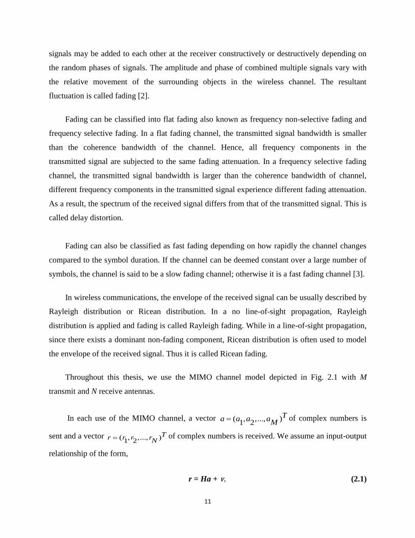
Throughout this thesis, we use the MIMO channel model depicted in Fig. 2.1 with M
transmit and N receive antennas.
In each use of the MIMO channel, a vector ( , ,..., )1 2
Ta a a aM
of complex numbers is
sent and a vector ( , ,..., )1 2
Tr r r rN
of complex numbers is received. We assume an input-output
relationship of the form,
r = Ha + v, (2.1)

12
where H is an M N matrix represents the scattering effects of the channel and is given by,
11 1
21 2 ,
1
h hM
h hMH
h hNMN
(2.2)
Figure 2.1: Multiple Input Multiple Output (MIMO) channel model.
where ijh is the complex channel gain between transmitter j and receiver i. Each channel gain
ijh is assumed to be independently identically distributed (i.i.d) zero mean complex Gaussian
random variable with unit variance [4], and 1 2( , ,..., )T
Nv v v v is the noise vector, we assume
throughout that v is a complex Gaussian random vector with i.i.d. elements ~ (0,1)iv CN . It is
assumed that H and v are independent of each other and of the data vector a. We assume also that
the receiver has a perfect knowledge of the channel realization H, while the transmitter has no
such channel state information (CSI). Receiver's possession of CSI is justified in cases where the
channel is a relatively slowly time-varying random process; see [5] for a discussion of this point.
2.4 The Symbols Detection Problem
The symbol detection problem considered in this thesis is the problem of estimating the
MIMO channel input vector with a given the received vector r under the assumption that the

13
receiver has perfect knowledge of H. This decision is made on a symbol by symbol basis without
taking into account any statistical dependencies that may be present in the sequence of vectors a.
In other words, we exclude coding across the time dimension and consider only the modulation-
demodulation problem as depicted in Fig. 2.2. The goal is to minimize the probability of decision
error
'
e rP = P a a , (2.3)
where ˆ ˆ ˆ ˆ T
1 2 Ma = (a ,a ,...,a ) is the demodulator's estimate of a.
Figure 2.2: Modulation, transmission and decision in MIMO wireless systems.
We study the above detection problem under additional assumptions on the input vector
which are given by,
Each element of a belongs to a common modulation alphabet A,
, 1, , Mai A i M a A Typically, A will be a QAM alphabet such as
1 2 1,A A jA A and 2A are integers as in the case of 4-QAM.
We will assume that symbols in A have equal a priori probabilities.
The vector a is a random vector over MA such that
{ }aa I
MM
,
(2.4)
where is a constant, MI is the identity matrix of size M, {.} is the expectation operator and
+a denotes Hermitian transpose of a. Assumption (2.4) implies that the elements of a are
uncorrelated and each has energy,
2{ } /a M
i .
(2.5)
Modulator MIMO
Channel
Demodulator aa r
14
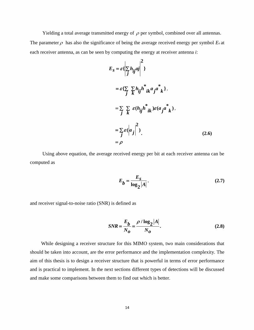
Yielding a total average transmitted energy of per symbol, combined over all antennas.
The parameter has also the significance of being the average received energy per symbol Es at
each receiver antenna, as can be seen by computing the energy at receiver antenna i:
2
{ }E h ajs ijj
* *{ }h h a a
ij ik j kj k ,
* *( ) ( )h h a a
ij ik j kj k ,
2( )a
jj
.
(2.6)
Using above equation, the average received energy per bit at each receiver antenna can be
computed as
log
2
EsEb A ,
(2.7)
and receiver signal-to-noise ratio (SNR) is defined as
/ log2
E AbSNR
N No o
.
(2.8)
While designing a receiver structure for this MIMO system, two main considerations that
should be taken into account, are the error performance and the implementation complexity. The
aim of this thesis is to design a receiver structure that is powerful in terms of error performance
and is practical to implement. In the next sections different types of detections will be discussed
and make some comparisons between them to find out which is better.

15
2.5 Detection Algorithms
For the signal detection problem defined in the previous section, one decision rule is the
MAP rule defined as,
ˆ arg max{Pr( | )}a a r is received
Ma A
.
(2.9)
It is well-known that the MAP rule minimizes the probability of error Pe (see, e.g., [6, p.
324]).
Another decision rule is the maximum likelihood (ML) rule defined as
Set ˆa a MA for some a so that
( | ) ( | )f r a f r a for allM
a A , (2.10)
where
f r a Ha rN N NN oo
1 1 2( | ) exp{ }
(2 )
,
(2.11)
Since ~ (0, )o NV CN N I .Thus, the ML rule here reduces to
a Ha r
Ma A
2ˆ arg min{ }
.
(2.12)
In fact, ML rule is equivalent to MAP rule if all the source symbols are equally likely to be
transmitted a-priori. Although MAP rule offers optimal error performance, it suffers from
complexity issues. It has exponential complexity in the sense that the receiver has to
consider MA possible symbols for an M transmitter antenna system. For example, if 64-QAM is
used with 4 transmit antennas, then a straightforward implementation of the MAP detector needs
to search over 464 = 16,777,216 symbols. Similar complexity problems apply to ML detectors.
In order to solve the detection problem in MIMO systems, research has focused on
suboptimal receiver models which are powerful in terms of error performance and in the same
time are practical for implementation purposes. One such receiver is the V-BLAST receiver
which utilizes a layered architecture and applies successive cancellation by splitting the channel
vertically [7].

16
As pointed out in Section 2.3, the decision rule that minimizes the probability of symbol
error Pe, which is defined in Eq. (2.3), is the ML rule given by Eq. (2.12). However, since the
ML rule requires searching over MA symbols, it is not practical when this number is large. In this
chapter, we review a number of suboptimal symbol detection rules that have been proposed as
practical alternatives to the ML rule.
2.6 Linear Receivers
Linear receivers are the class of receivers for which the symbol estimate a is given by a
transformation of the received vector r of the form
a Q Wrˆ ( ) , (2.13)
where W is a matrix that may depend on H and Q is a quantizer (also called slicer) that maps its
argument to the nearest signal point in M
A (using Euclidian distance) [8].
2.6.1 Zero-Forcing (ZF) Receiver
Zero-Forcing (ZF) receiver is a low-complexity linear detection algorithm that outputs
a Q a
ZFˆ ˆ( ) ,
(2.14)
where
a H r
ZF ,
(2.15)
and H denotes the Moore-Penrose pseudo inverse [9] of H, which is a generalized inverse that
exists even when H is rank-deficient.
For a more realistic performance estimation of the ZF receiver, we show in Fig. 2.3 the
simulation results for a (M, N) = (8, 8) system with 16-QAM modulation. Theb oE / N , defined
by Eq. (2.8), ranges between 2 dB and 14 dB in steps of 2 dB. The symbol error rate SER is
calculated by performing 10,000 trials at each b oE / N point. A new realization of H was chosen
in each trial and for each /b oE N value.

17
Eb/No (dB)
2 4 6 8 10 12 14
SE
R
0.0001
0.001
0.01
0.1
1
10
VBLAST/ZF
VBLAST/LLSE
ZF
LLSE
Figure 2.3: SER of ZF, LLSE, VBLAST-ZF, and VBLAST-LLSE receivers without coding.
2.6.2 Linear Least Square Estimation (LLSE) Receiver
The LLSE receiver is a receiver that outputs the estimate
a Q aLLSEˆ ˆ( )
, (2.16)
where ˆLLSEa is a linear estimator given by
a WrLLSE
,
(2.17)
where W is chosen to minimize
2Wr a .
For the model here, where H and v are Gaussian, the LLSE estimator matrix is given by [8],
1( )W H HH N Io NM M
. (2.18)

18
For a more realistic performance estimation of the LLSE receiver, we show in Fig. 2.3 the
simulation results for a (M, N) = (8, 8) system with 16-QAM modulation. Theb oE / N , defined
by Eq. (2.8), ranges between 2 dB and 14 dB in steps of 2 dB. The symbol error rate SER is
calculated by performing 10,000 trials at each b oE / N point. A new realization of H was chosen
in each trial and for eachb oE / N value. We observe that LLSE performs slightly better than ZF.
2.7 V-BLAST System
The first proposed algorithms were the Diagonal Bell laboratories layered space-time (D-
BLAST) and V-BLAST [15]. While the D-BLAST achieves the full MIMO capacity, it is more
complex as compared to the V-BLAST, which, despite its simplicity, achieves a significant
portion of the full MIMO capacity. V-BLAST is a detection algorithm to the receipt of MIMO
systems. Independent data can be transmitted simultaneously over multiple transmit antennas,
the data rate will increase proportional to the number of transmit antennas and the same band of
frequency used for every transmission which leads to high spectral efficiency [13]. Its principle
is quite simple, first it detects the most powerful signal (highest SNR), and then it regenerates the
received signal from this user from available decision. Then, the signal regenerated is subtracted
from the received signal and with this new sign; it proceeds to the detection of the second user's
most powerful signal, since it has already cleared the first signal and so forth. This gives less
interference to a vector received [16].
Although the detection algorithm for V-BLAST is based on the concept of multi-user
detection, it is single user detection. V-BLAST architecture was first proposed by Foschini to
increase capacity while exploiting multipath fading [5].
This section covers the basic principles and detection algorithms for V-BLAST with
various detection techniques.

19
2.7.1 V-BLAST Architecture
The BLAST architecture is one of the earliest communication systems that proposed to
take advantage of the high capacity of MIMO channels. It can achieve high spectral efficiencies
by making spatially multiplexing coded or uncoded symbols over the MIMO channel [18].
Therefore, the symbols can transmitted through M antennas and each receiving antenna receives
a superposition of faded symbols. The transmission for V-BLAST is done by splitting the data
streams to M sub- stream layers. So, the layers are arranged horizontally across time and space.
At the receiver end, as mentioned previously, the received signals at each receive antenna are a
superposition of M faded symbols plus additive white Gaussian noise (AWGN).The detection
process is performed vertically for each received vector.
Figure 2.4 shows a block diagram of the V-BLAST architecture. There are M transmit
antennas and N receive antennas, where N ≥M. The data is first de-multiplexed into layers, or
parallel sub-streams, and each layer is transmitted from a different antenna. Each antenna
transmits the data layers simultaneously in the same frequency band. The channel is assumed to
be quasi-static, flat, Rayleigh fading. The receivers operate co-channel where the signal at each
receiver contains superimposed components of the transmitted signals.
The V-BLAST system model can be represented in matrix notations. The vector of
transmitted symbols, at time k, is represented by
[ (1) (2) ... ( )]
Tx x x x Mk k k k .
(2.19)
Each receive antenna receives signals from all M transmit antennas. The received signal
during the kth
time interval is expressed as,

20
Figure 2.4: Block diagram of V-BLAST architecture
r HX Vk k k ,
(2.20)
where H is the channel matrix given by (2.2), and vk is the noise vector given by
[ (1) (2) ( )]
Tv v v v Nk k k k ,
(2.21)
where v is assumed to be i.i.d. additive white Gaussian noise with zero mean and covariance
matrix2
nI .
V-BLAST detection uses of linear nulling techniques (such as ZF or LLSE) or non-linear
methods like symbol cancellation. In each time interval there is one sub stream is considered to
be the desired signal and all the others are interferers. Nulling is obtained by linearly weighting
(W) the received signals.
The Main Steps for V-BLAST detection are:
1. Ordering: choosing the best channel.
2. Nulling: using ZF, LLSE or ML.
3. Slicing: making a symbol decision.
4. Canceling: subtracting the detected symbol.
5. Iteration: going to the first step to detect the next symbol [14].

21
Here, different techniques used for performance measure are illustrated (Namely, Maximum
Likelihood (ML) detector, Zero forcing (ZF), and Linear Least Square Estimation (LLSE)).
i. Maximum Likelihood (ML) Receiver:
The ML receiver performs optimum vector decoding and is optimal in the sense of
minimizing the error probability. ML receiver is a method that compares the received signals
with all possible transmitted signal vectors which are modified by channel matrix H and
estimates transmit symbol vector x according to the Maximum Likelihood principle.
The Maximum Likelihood try to find x which minimizes, ˆ2
J = Y - H× x , if MIMO is 2×2
J becomes:
ˆ
ˆ
2y h h x1 11 12 1
J = -y h h x2 21 22 2
(2.22)
Note that y is the constellation points, x is a received vector and H is a channel matrix.
And so on, where the minimization is performed over all possible transmit estimated symbol
vectors x. Although ML detection offers optimal error performance, it suffers from a very high
complexity.
ii. V-BLAST Zero Forcing (ZF) characteristic:
By using ZF technique, we can reduce the decoding complexity of the ML receiver
significantly. It has a simple linear receiver with low computational complexity and suffers from
noise enhancement. It works best with high values of SNR. [19]
The zero forcing try to find a matrix W which satisfies WH=I. so to achieve this constraint the W
matrix must satisfy the following equation:
-1H H
W = H × H (2.23)
The V-BLAST/ZF algorithm is a variant of V-BLAST derived from ZF rule. [7]

22
In Fig. 2.5 the steps of V-BLAST/ZF were shown, where H denotes the Moore-Penrose
pseudo inverse of H [9], ( )i jW is the jth
row of , (.)iW Q is a quantizer to the nearest constellation
point, ( )ikH denotes the k
th column of H ,
ikH denotes the matrix obtained by zeroing the
columns 1, 2 ,..., ik k k of H , and k
H denotes the pseudo-inverse of ik
H .
Figure 2.5: V-BLAST/ZF Detection Algorithm.
In the above algorithm, Eq. (2.24c) determines the order of channels to be detected; Eq.
(2.24d) performs nulling and computes the decision statistic; Eq. (2.24e) slices computed
decision statistic and yields the decision; Eq. (2.24f) performs cancellation by decision feedback,
and Eq. (2.24g) computes the new channel matrix for the next iteration.
V-BLAST/ZF may be seen as a successive-cancellation scheme derived from the ZF
scheme discussed in Section 2.5.1. The ZF rule creates a set of sub-channels by forming
ˆ + +
ZFa =(H H)a+H V , as in Eq. 2.15. The jth
such sub-channel has noise variance2
+
j o(H ) N .
The order selection rule prioritizes the sub-channel with the smallest noise variance.

23
For a more realistic performance estimation of the V-BLAST/ZF receiver, we show in
Fig. 2.3 the simulation results for a (M, N) = (8, 8) system with 16-QAM modulation.
Theb oE / N , defined by Eq. (2.8), ranges between 2 dB and 14 dB in steps of 2dB. The symbol
error rate SER is calculated by performing 10,000 trials at each b oE / N point. A new realization
of H was chosen in each trial and for each b oE / N value. Result of this simulation is very similar
to an experiment performed in a real laboratory environment which is reported in [7].
We observe that V-BLAST/ZF performs significantly better than both ZF and LLSE receivers.
iii. V-BLAST with Linear Least Square Estimation (LLSE):
The LLSE receiver provides a balanced solution to the problem of reducing the effects of
both interference and channel noise enhancement effect plaguing the ZF equalizer, whereas the
ZF receiver removes only the interference components [19].
This implies that the mean square error between the transmitted symbols and the estimate of
the receivers is minimized. Hence, LLSE is superior to ZF in the presence of noise. Some of the
important characteristics of LLSE detector are simple linear receiver.
The LLSE approach tries to find a coefficient W which minimizes,
EH
Wy - x Wy - x , (2.24)
where E{x} is the expectation value of x.
And find,
1( )W H HH N Io NM M
(2.25)
The V-BLAST/LLSE algorithm is a variant of V-BLAST where the weighting matrix is chosen
according to the LLSE rule [10].

24
Figure 2.6: V-BLAST/LLSE Detection Algorithm.
For a more realistic performance estimation of the V-BLAST/LLSE receiver, we show in
Fig. 2.3 the simulation results for a (M, N) = (8, 8) system with 16-QAM modulation.
The /b oE N , defined by Eq. (2.8), ranges between 2 dB and14 dB in steps of 2 dB. The symbol
error rate SER is calculated by performing10, 000 trials at each b oE / N point. A new realization
of H was chosen in each trial and for each b oE / N value. We observe a slight improvement
compared to the performance of V-BLAST/ZF.
Figure 2.7 compares the symbol error rate (SER) versus signal to noise ratio for different
versions of the V-BLAST algorithm. The Ordered LLSE algorithm yields the best SER
performance, whereas the unordered ZF algorithm yields the worst. The Ordered Algorithm
detects the strongest signal first. As a result, the strongest interference is cancelled first. On
average, this leads to improved BER performance in the sequentially detected layers.
The LLSE nulling criteria utilizes knowledge of the signal to noise ratio to improve performance.

25
Eb/No (dB)
2 4 6 8 10 12 14
SE
R
0.001
0.01
0.1
1
VBLAST/ZF ORDERED
VBLAST/ZF UNORDERED
VBLAST/LLSE ORDERED
VBLAST/LLSE UNORDERED
Figure 2.7: Different V-BLAST Algorithms.
2.8 V-BLAST/MAP Detection Algorithm
In this section, we describe a new symbol detection algorithm for MIMO channels, which
is called V-BLAST/MAP that combines the features of V-BLAST and MAP rules. This
algorithm uses the layered structure of V-BLAST, but uses a different strategy for channel
processing order, inspired by the MAP rule. The complexity of the V-BLAST/MAP is higher
than that of V-BLAST; however, the performance improvement is also significant. Simulations
show that V-BLAST/MAP achieves symbol error rates close to the optimal maximum likelihood
(ML) scheme while retaining the low-complexity nature of the V-BLAST.
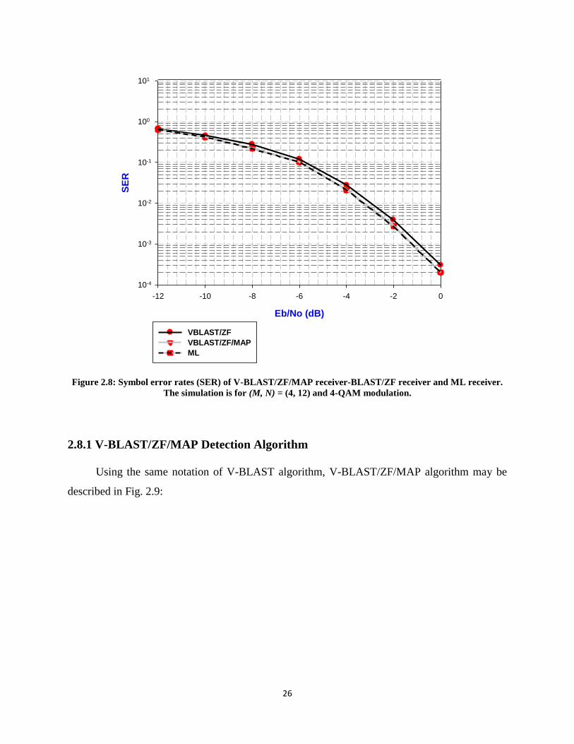
Fig. 2.8 depicts the error performance of V-BLAST/ZF/MAP versus those of V-
BLAST/ZF and ML for the case of (M, N) = (4, 12) and 4-QAM modulation with
alphabet A jA .
26
Eb/No (dB)
-12 -10 -8 -6 -4 -2 0
SE
R
10-4
10-3
10-2
10-1
100
101
VBLAST/ZF
VBLAST/ZF/MAP
ML
Figure 2.8: Symbol error rates (SER) of V-BLAST/ZF/MAP receiver-BLAST/ZF receiver and ML receiver.
The simulation is for (M, N) = (4, 12) and 4-QAM modulation.
2.8.1 V-BLAST/ZF/MAP Detection Algorithm
Using the same notation of V-BLAST algorithm, V-BLAST/ZF/MAP algorithm may be
described in Fig. 2.9:

27
Figure 2.9: V-BLAST/ZF/MAP Detection Algorithm.
Here the vectorsT
i i1 i2 iMy =(y ,y ,..., y ) and T
i i1 i2 iMs = (s ,s ,...,s ) are the counterparts of those
in Eq.'s (2.14) and (2.15) in the ZF detector. In (2.22e), ijf is a density function given by
f y s y sij ij ij ij ij
j j
21 1( / ) exp
2 2
,
(2.27)
where 2
2
j o i jσ = N (W ) . In (2.26e) and (2.26f), the index j ranges over all elements of
1,2,...,M excluding those in 1 i-1k ,...,k ,i.e., j 1 i-11,...,M / k ,...,k .

28
V-BLAST/ZF/MAP algorithm is identical to V-BLAST/ZF except for the ordering in
which symbols are detected. Instead of selecting the next symbol to be detected according to the
rule (2.24c), here the set of all potential symbol decisions are ranked with respect to their a-
posteriori probabilities of being correct, as estimated by ijp . Thus, it is important to emphasize
that ijp 's are not true MAP probabilities but approximations to how probable it is that
ij js = a .
The approximation is due to the omission in calculations of the cross correlations between the
noise terms ij ij ijz = y - s on the component sub channels. Notice that the index permutation
1 2 M(k ,k ,...,k ) produced by V-BLAST/ZF/MAP depends on both H and r, unlike V-BLAST/ZF
where the permutation depends only on H.
The complexity of V-BLAST/ZF/MAP is increased with respect to that of V-BLAST/ZF
by the computation done in step (2.26e). The order of complexity of computing ijp is
roughly O A for any fixed j, and upper bounded by O M A when considered as a whole.
This computation can be further simplified by approximating the denominator of (2.26e) but that
issue is not explored in this thesis.
One major point about complexities of V-BLAST/ZF and V-BLAST/ZF/MAP is that in
the former allows pre-computation of all weighting vectors (which can be used repeatedly as
long as H is fixed) whereas in the latter the weighting vector must be computed in real-time since
it also depends on r. This increased complexity of V-BLAST/ZF/MAP is justified by
performance improvements as illustrated later in this section.
For a more realistic performance estimation of the V-BLAST/ZF/MAP receiver, we show
in Fig. 2.11 the simulation results for a (M, N) = (8, 8) system with 16-QAM modulation.
The /b oE N , defined by Eq. (2.8), ranges between -4 dB and 4 dB in steps of 2dB. The symbol
error rate SER is calculated by performing 10,000 trials at each b oE / N point. A new realization
of H was chosen in each trial and for each b oE / N value. We observe that V-BLAST/ZF/MAP
performs significantly better than both V-BLAST/ZF and V-BLAST/LLSE receivers.

29
2.8.2 V-BLAST/LLSE/MAP Detection Algorithm
In this section, we use the LLSE technique in order to compute weighting matrix.
Then, V-BLAST/LLSE/MAP algorithm may be described in Fig.2.10:
Figure 2.10: V-BLAST/ZF/MAP Detection Algorithm.
Eb/No (dB)
-4 -2 0 2 4
SER
0.1
1
10
VBLAST/ZF
VBLAST/LLSE
VBLAST/ZF/MAP
VBLAST/LLSE/MAP
Figure 2.11: Symbol error rate (SER) of VBLAST/ZF/MAP receiver, VBLAST/LLSE/MAP receiver,
VBLAST/ZF receiver and VBLAST/LLSE receiver.

30
For a more realistic performance estimation of the V-BLAST/LLSE/MAP algorithm, we
show in Fig. 2.11 the simulation results for a (M, N) = (8, 8) system with 16-QAM modulation.
The /b oE N ranges between -4 dB and 4 dB in steps of 2db. The symbol error rate SER is
calculated by performing 10,000 trials at each /b oE N point. A new realization of H was chosen
in each trial and for eachb oE / N value.
2.9 Conclusion
In this chapter, the MIMO channel model was introduced. MIMO symbol detection
problem is stated and some brief description of previous detection algorithms is presented. The
Ordered LLSE and ZF algorithms was also presented, The V-BLAST detection algorithm with
various detection techniques was presented and comparison between them was made to observe
that the LLSE algorithm performs slightly better than ZF algorithm, V-BLAST/ZF performs
significantly better than both ZF and LLSE, V-BLAST/LLSE performs slight better compared to
the performance of V-BLAST/ZF and V-BLAST/ZF/MAP performs significantly better than
both V-BLAST/ZF and V-BLAST/LLSE.
However, we may state as the main conclusion of this chapter that V-BLAST/MAP offers
significantly better SER performance than V-BLAST and has efficiency close to ML with
relatively low complexity.

31
References
[1] P. W. Wolniansky, G. J. Foschini, G. D. Golden, and R. A. Valenzuela,”V-blast: An
architecture for realizing very high date rates over the rich-scattering wireless channel," Proc.
URSI ISSSE, pp. 295-300, 1998.
[2] T.Rapaport, Wireless communication: Principles and Practice, 2nd ed. Prentice Hall, 2001
[3] J. Proakis, Digital communication, 4thed. New York: McGraw-Hill.
[4] G.Foschini and M.Gans,” On limits of wireless communications in a fading environment
when using multiple antennas,” Wireless Personal Communications, vol.6, pp.311-35, no.3,
March 1998.
[5] G. J. Foschini, “Layered space-time architecture for wireless communication in a fading
environment when using multiple antennas," Bell Labs Tech. J., vol. 1, pp. 41-59, Autumn 1996.
[6] S. Haykin, Communication Systems, John Wiley & Sons, Inc., 2001.
[7] G. D. Golden, G. J. Foschini, R. A. Valenzuela, and P. W. Wolniansky, “Detection algorithm
and initial laboratory results using v-blast space-time communication architecture," Electronic
Letters, vol. 35, pp. 14-16, January 1999.
[8] H. Bolcskei and A. J. Paulraj, The Communications Handbook, CRC Press, 2nd ed. J.
Gibson, 2002.
[9] G. H. Golub and C. F. V. Loan, Matrix computations, John Hopkins University Press,
Baltimore, 1983.
[10] R. L. Cupo., G. D. Golden, C. Martin, K. L. Sherman, N. R. Sollen bergen,J. H. Winters,
and P. W. Wolniansky, “A four-element adaptive antenna array for is-136 pcs base stations,"
(Phoenix), pp. 1577-1581, IEEE Vehicular Technology Conference, May 1997.
[11] A. Bhargave, R. J.P. de Figueiredo, and T. Eltoft, “A detection algorithm for the VBLAST
system,” IEEE Global Telecommunication Conference, vol. 1, pp. 494-498, Nov. 2001.
[12] D. W. Waters, “Signal detection strategies and algorithms for multiple-input multiple-output
channels,” Georgia Institute of Technology December 2005.

32
[13] R. Trepkowski “Channel estimation strategies for coded MIMO systems,” Blacksburg,
Virginia, 2004.
[14] S. A. Joshi, T. S. Rukmini, H. M. Mahesh, “Performance analysis of MIMO technology
using V-BLAST technique for different linear detectors in a slow fading channel,” IEEE
International Conference on Computational conference on Computational Intelligence and
Computing Research (ICCIC‟2010).978-1-4224-5966-7/10. p 453-456.
[15] G.J. Foschini, “Analysis and performance of some basic space-time architectures,” IEEE
Journal Selected Areas Communication, Vol. 21, N. 3, pp. 281-320, April 2003.
[16] G.J Foschini, “Simplified processing for high spectral efficiency wireless communication
employing multi-element arrays,” IEEE Journal on Selected Areas in Communications, vol. 17,
no 11, pp. 1841-1852, November 1999.
[17] Y. Yapici, “V-BLAST/MAP: A new symbol detection algorithm for MIMO channels” A
Thesis Submitted to The Department of Electrical and Electronics Engineering and The Institute
of Engineering and Science of Bilkent University in Partial Fulfillment of The Requirements for
The Degree of Master of Science, January 2005.
[18] N. Sinha, R. Bera, and M. Mitra. “Capacity and V-blast techniques for MIMO wireless
channel,” Theoretical and Applied Information Technology Journal (JATIT), vol. 14, no. 1,
2010.
[19] D. Seethaler, H. Artes, and F. Hlawatsch “Detection techniques for MIMO spatial
multiplexing systems,” Institute of Communications and Radio-Frequency Engineering, Vienna
University of Technology, vol. 122, no. 3, pp. 91–96, March 2005.

33
Chapter 3
Turbo Codes
3.1 Introduction
Since Shannon‟s work, the focus of coding theory was aiming to find a way to place
2k codewords in n-dimensional space without overlapping. One attempt was the Hamming code,
which is the first error correcting code, was able to correct a single error in a block of seven
encoded bits. The (7, 4) Hamming code contains 24 codewords with 7 symbols and has a rate
equal to 4 7 . The code rate r is defined as the ratio of k, the number of information symbols
transmitted per codeword, to n, the total number of symbols transmitted per codeword. Other
attempts to solve the problem presented by coding theorists have introduced the block codes
(such as Golay, BCH, and Reed-Solomon codes) and convolutional codes, but prior to the early
1990‟s, no practical techniques achieved the full promise of Shannon‟s predictions. Turbo codes
are able to integrate structured codes in a random manner, which achieves very nearly Shannon‟s
capacity limit; this lead to a significant increase in power efficiency compared to previous block
and convolutional coding schemes. Turbo codes get their name because the decoder uses
feedback, like a Turbo engine.
The original “Turbo code” uses two recursive systematic convolutional (RSC) encoders
concatenated in parallel and separated by a pseudo-random interleaver [1]. Each RSC encoder
with a rate 1 2 produces a set of systematic and parity bits. The systematic bits are same as input
bits; the parity bits calculated using the input bits, the state of the encoder, and the generator
matrix. Therefore, two set of systematic bits generated. Then, to decrease the redundancy, the
interleaved systematic bits from the second RSC encoder are punctured, or removed, before

34
transmission. The overall rate of the Turbo code can increased from 1 3 to 1 2 by alternately
puncturing the parity bits from each of the constituent encoders. The resulting code has a
complex structure and appears quite random. This characteristic of the code results in good
performance, particularly at low signal-to-noise ratios (SNRs). The overall code, however, is
broken down into its constituent parts at each decoder, and each constituent code can be decoded
relatively easily because of its inherent structure. Each decoder operates on the systematic and
parity bits associated with its constituent encoder and produces soft outputs of the original data
bits in the form of a posteriori probabilities (APPs). The decoders then share their respective soft
information in an iterative fashion.[1]
Although Turbo codes are a new form of error correction, their foundation is rooted in
coding theory. This chapter presents the development of Turbo codes and discusses the
theoretical background necessary to understand their application. The algorithms used to decode
Turbo codes are also described, and performance factors which influence Turbo-coded systems
are explained and illustrated.
Turbo code is a class of high performance forward error correction codes, which can approach
the Shannon limit. Turbo code is nowadays competing with LDPC code, which provides similar
performance.[33]
3.2 Channel Codes:
3.2.1 Block Codes
Block codes are based on finite field arithmetic and abstract algebra and can used to correct
or detect errors. Referred to this code as (n, K) block code where K is information bits, n
code bits and (n-K) redundant bits. Some of commonly used block codes are Hamming code,
Golay code, BCH codes, and Reed Solomon code.
3.2.2 Convolutional Code:
Convolutional code developed with strong mathematical structure and it is used for real time
error correction. Convolutional code converts the entire data stream into one single code

35
word. The encoded bits depend not only on the current K input bits but also on past input
bits.
3.2.3 Turbo Codes:
Turbo code is a class of high performance forward error correction codes, which can approach
the Shannon limit. Turbo code is nowadays competing with LDPC code, which provides similar
performance. [33]
There are three main types of Turbo codes as follow:
Parallel concatenated convolution code PCCC
Serial concatenated convolution code SCCC
Hybrid concatenated convolutional code HCCC.
Here in this research PCCC is what we are considered for illustration purpose.
Parallel concatenated convolution code PCCC
The parallel-concatenated convolution codes (PCCCs) consists of recursive and
systematic convolutional (RSC) codes, which an interleaver separates Fig 3.1. So, the first
encoder is RSC and has trellis terminated (tail bits are added) and second has un-terminated
trellis (no tail bits). The separated interleaver is random and the properties of the interleavers
are very critical point on the performance of the Turbo code. The C(s) is a systematic output,
C(p1) is a first parity output and C(p2) is a second parity output of PCCC encoder.
Figure 3.1: The parallel-concatenated convolution codes by a rate of 1/3.
36
3.3 Convolutional Codes
Convolutional codes are one technique from the general class of channel codes, which
permit reliable communication of an information sequence over a channel that adds noise,
introduces bit errors, or otherwise distorts the transmitted signal. Elias introduced convolutional
codes in 1955 [2], [3]. Convolutional codes play a role in low-latency applications such as
speech transmission and as constituent codes in Turbo codes [4], [5].
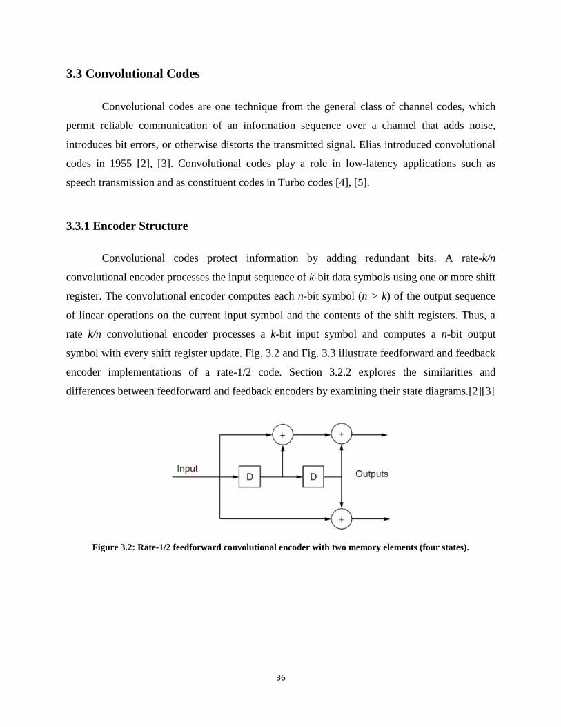
3.3.1 Encoder Structure
Convolutional codes protect information by adding redundant bits. A rate-k/n
convolutional encoder processes the input sequence of k-bit data symbols using one or more shift
register. The convolutional encoder computes each n-bit symbol (n > k) of the output sequence
of linear operations on the current input symbol and the contents of the shift registers. Thus, a
rate k/n convolutional encoder processes a k-bit input symbol and computes a n-bit output
symbol with every shift register update. Fig. 3.2 and Fig. 3.3 illustrate feedforward and feedback
encoder implementations of a rate-1/2 code. Section 3.2.2 explores the similarities and
differences between feedforward and feedback encoders by examining their state diagrams.[2][3]
Figure 3.2: Rate-1/2 feedforward convolutional encoder with two memory elements (four states).

37
Figure 3.3: Rate-1/2 feedback convolutional encoder with two memory elements (four states).
3.3.2 Equivalent Encoders
Convolutional encoders are finite-state machines. Hence, state diagrams provide
considerable behavior of convolutional codes. Fig. 3.4 and Fig. 3.5 provide the state diagrams for
the encoders of Fig. 3.2 and Fig. 3.3; respectively. The states are labeled so that the least
significant bit is the one residing in the leftmost memory element of the shift register. The
branches are labeled with the 1-bit (single-bit) input and the 2-bit output separated by a comma.
Figure 3.4: State diagram for rate-1/2 feedforward convolutional encoder of Fig. 3.2.

38
Figure 3.5: State diagram for rate-1/2 feedback convolutional encoder of Fig. 3.3.
The two encoders are equivalent produce the same set of possible output sequences (or
codewords). So, the two equivalent encoders have the same set of possible output sequences, but
may implement different mappings from input sequences to output sequences. The feedforward
shift register has a finite impulse response, and the feedback shift register has an infinite impulse
response. This difference is not particularly important for convolutional codes decoded with
Viterbi, but it is extremely important to convolutional encoders used as constituents in Turbo
codes, which are constructed by concatenating convolutional codes separated by interleavers.
Only feedback encoders (with infinite impulse responses) are effective constituents in Turbo
codes. Thus, equivalent encoders can produce dramatically different performance as constituents
in Turbo codes, depending on whether or not they meet the requirement for an infinite impulse
response.[2][3]
3.3.3 Convolutional Codes Decoding
There are three families of decoding algorithms for convolutional codes: sequential,
Viterbi, and maximum a posteriori (MAP). Wozencraft proposed sequential decoding in 1957
[6]. Fano in 1963 and Zigangirov in 1966 further developed sequential decoding [7],[8]. Viterbi
originally described the decoding algorithm that bears his name in 1967 [9]. See also Forney‟s
work introducing the trellis structure and showing that Viterbi decoding is maximum-likelihood
in the sense that it selects the sequence that makes the received sequence most likely [10], [11].
In 1974, Bahl et al. [12] proposed MAP decoding, which explicitly minimizes bit (rather than

39
sequentially) error rate. Compared with Viterbi, MAP provides a negligibly smaller bit error rate
(and a negligibly larger sequence error rate). These small performance differences require
roughly twice the complexity of Viterbi, making MAP unattractive for practical decoding of
convolutional codes. However, MAP decoding is crucial to the decoding of Turbo codes. For the
application of MAP decoding of Turbo codes, see the original paper on Turbo codes by Berrou et
al. [13] and Benedetto et al.‟s specific discussion of the basic Turbo decoding module [14].
Trellis Diagrams
The state diagrams of Fig. 3.4 and Fig. 3.5 illustrate what transitions are possible for a
particular state regardless of time. In contrast, trellis diagrams use a different branch for each
different symbol time. As a result, a trellis diagram more clearly illustrates long trajectories
through the states. Fig. 3.6 shows one stage (one symbol time) of the trellis diagram associated
with the rate-1/2 feedforward encoder of Fig. 3.2 and Fig. 3.4. Each column of states in the trellis
diagram includes everything in the original state diagram
Figure 3.6: One stage of the trellis diagram for rate-1/2 feedforward convolutional encoder of Figs. 3.2 and
3.4.
Hard versus Soft Decoding
For the AWGN channel, binary phase shift keying (BPSK) represents a binary 1 with 1
and a binary 0 with −1. These two transmitted values are distorted by additive Gaussian noise, so
that the received values will typically be neither 1 nor −1. A simple approach is to simply

40
quantize each received value to the closest of 1 and −1 and assign the appropriate binary value.
This method of decoding is called hard decoding, because the receiver makes a binary (hard)
decision about each bit before the Viterbi decoding. Hard decoding performs worse by about 2
dB than a more precise form of Viterbi decoding known as soft decoding [9]. Soft decoding
passes the actual or multi-level quantized received values to the Viterbi decoder. These values
are called soft values because hard decisions (binary decisions) have not been made to Viterbi
decoding. Soft Viterbi decoding is very similar to hard decoding, but branch and path metrics use
squared Euclidean distance rather than Hamming distance [10].
3.3.4 Free Distance
Free distance gives a good indication of convolutional code performance. The free
distance of a convolutional code is the minimum distance (either Hamming or Euclidean)
between two distinct valid output sequences.
Computation of Free Distance
The set of distances from a codeword to each of its neighbors is the same for all
codewords. Hence, the free distance is the distance from the all-zeros output sequence to its
nearest-neighboring codeword. A Viterbi decoding operation with some special restrictions
efficiently performs this computation. Viterbi decoding is performed on the undistorted all-zeros
received sequence, but the first trellis branch associated with the correct path is disallowed. Thus
prevented from decoding the correct sequence, the Viterbi algorithm identifies the nearest-
neighbor sequence. Since the received sequence is noiseless, the path metric associated with the
decoded sequence is the distance between that sequence and the all-zeros sequence, which is the
free distance. Figure 3.7 illustrates the computation of free Hamming distance using the Viterbi
algorithm for the encoder described in Fig. 3.2, Fig. 3.4, and Fig. 3.6. The disallowed branch is
shown as a dashed line. Only survivor branches are shown, and the thick branches indicate the
minimum distance survivor path. Below each column is the minimum survivor path metric,
which is called the column distance. The free distance is formally defined as the limit of the
column distance sequence as the survivor path length tends to infinity. This limit is 5 in Fig. 3.7.

41
In general, the minimum distance path need not be the shortest path. For encoders with more
states than the simple example of Fig. 3.7, there are typically several such paths having the same
minimum distance. The number of minimum distance paths is the number of nearest-neighbor
output sequences. This is sometimes called the multiplicity of the free distance. If two codes
have the same free distance, the code with the smaller multiplicity is preferred [5].
Figure 3.7: Free Hamming distance of the code described by Figs. 3.2, 3.4, and 3.6.
3.4 Turbo Code Encoding
3.4.1 Classification of Concatenated Codes
Concatenated codes can be classified as either parallel concatenated convolutional codes
(PCCCs or serial concatenated convolutional codes (SCCCs). The term “Turbo code” is often
associated with PCCCs and will be used to refer to PCCCs throughout the rest of this thesis.
PCCCs have two or more recursive systematic convolutional (RSC) encoders connected in
parallel with pseudo-random interleavers between them. Systematic encoding is desirable for
parallel concatenation because it has easy puncturing process. Feedforward implementations of
systematic convolutional codes do not generally have good distance properties, but feedback or
recursive implementations do. Thus, RSC can produce higher weight output codewords
compared to non-recursive, if the input information weight is low. This is a major advantage in a
PCCC system since low input weight codewords dominate the error events; RSC is generally
used for Turbo codes. The pseudo-random interleavers reduce the probability that both
constituent encoders will simultaneously produce low weight parity sequences. This technique
gives PCCCs their excellent performance despite the relatively small free distance of the
constituent codes.

42
Figure 3.8: Encoder structures for (a) PCCCs and (b) SCCCs [32].
Fig. 3.7 illustrates the encoder structures for PCCCs and SCCCs. The class of SCCCs
was investigated by Forney in [15]. For a frame size N, the key feature of SCCCs is that, unlike
PCCCs whose interleaver gain is fixed at -1N , the slope of the BER curve continues to decrease
as a function of -2N , -3N etc. Thus, SCCCs do not suffer from as shallow an error floor as
PCCCs. Although the outer code for SCCCs need not be recursive, the inner code must be
recursive in order to exploit the interleaver gain [16]. PCCCs are often chosen over SCCCs in
practice because they are less computationally complex given the same constituent codes; they
also have lower BERs than SCCCs at low SNRs.
3.4.2 Encoding Operation
Turbo encoding employs two or more identical constituent recursive systematic
convolutional (RSC) encoders separated by a pseudo-random interleaver. An example of a
constraint-length 3, RSC encoder with generator matrix octal
G = 7,5 is shown in Fig. 3.9.
The data bits kd are fed into the first encoder which generates a set of systematic and parity bits.
The data bits are passed to the second encoder after being permuted by a pseudo-random
interleaver. The second encoder also generates a set of systematic and parity bits. Because

43
sending two sets of systematic bits is redundant, the overall code is punctured by deleting the
second set of systematic bits. The resulting bit stream consists of a systematic bit from the first
encoder followed by the parity bits from the first and second encoders, respectively. This
technique results in an overall code rate of 1 3 . The code rate can be increased to 1 2 by
alternately puncturing the parity bits from each of the constituent encoders before transmission.
As the code rate increases, bandwidth efficiency improves; performance, however, is degraded
since the decoder has less information to use in making a decision.
In Fig.3.10 the Bit error rate performance was shown for a punctured Turbo code at rate R=1/2 ,
data block length 1000 bits,100 frames,4 iterations and a log-MAP decoder.
In Fig.3.11 the Bit error rate performance was shown for unpunctured Turbo code at rate
R=1/3, data block length 1000 bits, 100 frames, 4 iterations and a log-MAP decoder.
Fig. 9 and Fig.10 indicated that further iterations would yield significant improvements
and the unpuncture encoder has better bit error rate. For example in case of BER = 210 and at
2nd iteration, we have coding gain of 1 dB for the unpuncture code compared to the puncture
code.
Figure 3.9: A constraint-length 3, RSC encoder with generator matrix octal
G = 7,5 .

44
Eb/No (dB)
0.0 0.5 1.0 1.5 2.0
BER
10-4
10-3
10-2
10-1
100
Iteration 1
Iteration 2
Iteration 3
Iteration 4
Figure 3.10: Bit error rate of Turbo code with frame size = 1000, iteration=4, number of frames = 100,
puncture, and by using log-map decoding.

45
Eb/No (dB)
0.0 0.5 1.0 1.5 2.0
be
r
10-4
10-3
10-2
10-1
100
Iteration 1
Iteration 2
Iteration 3
Iteration 4
Figure 3.11: Bit error rate of Turbo code with frame size = 1000, iteration=4, number of frames = 100, un-
puncture, and by using log-map decoding.
Convolutional codes can be used to encode a continuous stream of data, but in this case
we assume that data are configured infinite blocks corresponding to the interleaver size. The
frames can be terminated - i.e. the encoders are forced to a known state after the information
block. The termination tail is then appended to the encoded information and used in the decoder.
We can regard the Turbo code as a large block code. The performance depends on the weight
distribution not only the minimum distance but the number of words with low weight. Therefore,
we want input patterns giving low weight words from the first encoder to be interleaved to
patterns giving words with high weight for the second encoder.

46
3.5 Spectral Thinning and Random Interleavers
The primary function of the interleaver is to improve the distance properties of the
concatenated coding scheme. In PCCCs, the ideal interleaver permutes input sequences that
generate low weight codewords from one encoder into input sequences that generate high weight
codewords from the other encoder. In SCCCs, the ideal interleaver permutes low weight
codewords from the outer encoder into input sequences generating high weight codewords from
the inner encoder.
To a lesser extent the interleaver also serves to reduce the correlation between the input
sequence and the parity bits associated with the interleaved input sequence. Because an
independence assumption is made on the sequence being decoded and the extrinsic information
related to the sequence, it is important to make sure that the input sequence and the parity bits
associated with the interleaved input sequence are as uncorrelated as possible. It was shown in
[17] that addressing this issue when designing interleavers improves the convergence properties
of PCCCs and SCCCs employing short interleavers. Long interleavers (i.e., length-N > 500)
selected randomly have been shown in [18] to have good correlation properties, as good as long
interleavers designed specifically for those properties. Low weight codewords in a Turbo coding
scheme are generated in a two-step process. In the first step, an input sequence that begins with
one of the constituent coders in the all-zero state and returns that encoder to the all-zero state at
the end of the input sequence is encoded. The parity sequence generated by such an input
sequence terminates when the last non-zero bit of the input sequence is encoded. If the distance
between the first and last non-zero bit of this terminating input sequence is small, then the
codeword it generates will have relatively low Hamming weight. In the second step, either the
input sequence itself or the parity sequence it generates (in the case of a PCCC or SCCC,
respectively) is interleaved so that another high weight codeword is generated by the other
constituent encoder.

47
Example 3.1
Assuming that the parallel concatenated coding scheme in Fig. 3.8 employs as its
constituent encoders the recursive convolutional encoder shown in Fig. 3.12, the upper encoder
is terminated by the length-14 input sequence
Figure 3.12: Recursive convolutional encoder with three delay states and overall rate
=[0 0 1 0 1 1 0 0 0 0 0 0 0 0]m
and generates the parity sequence
1 = [0 0 1 1 1 1 0 0 0 0 0 0 0 0]y
If m is interleaved into
= [1 1 0 0 0 1 0 0 0 0 0 0 0 0],m
the lower encoder in Fig. 3.7 is also terminated and generates the parity sequence
2 = [1 0 1 1 0 1 0 0 0 0 0 0 0 0]y
The Hamming weight of the overall codeword generated in this case is the Hamming weight of
m + y1 + y2 = 3 + 4 + 4 = 11.
However, if m is interleaved into
= [1 0 0 1 0 0 0 1 0 0 0 0 0 0],m
the lower encoder in Fig. 3.8 is not terminated and generates the parity sequence
48
2 = [1 1 0 0 0 1 1 0 1 0 0 1 0 1]y
In this case the Hamming weight of m + y1 + y2 = 3 + 4 + 7 = 14. Furthermore, the
Hamming weight of the parity sequence y2 would increase with increased block length since the
input sequence [1 0 0 1 0 0 0 1]m did not terminate the lower encoder.
Because of the infinite impulse response of the constituent recursive convolutional encoders and
the use of a random interleaver to couple the concatenated encoders, relatively few low weight
codewords exist in a Turbo coding scheme. This phenomena, described as “spectral thinning” in
[17], is the cause of the very low BERs of Turbo coding schemes at low SNRs.
It is well known that the slope of the BER of a PCCC or SCCC is very steep at low and
medium SNRs (the “waterfall” region of the error performance curves) but flattens out
dramatically once the BER has converged to the error floor. The error floor is caused by error
patterns corresponding to low weight codewords not being corrected by the decoder. The
expected number, or multiplicity, of low weight codewords for a particular Turbo coding scheme
employing a randomly generated interleaver decrease at a rate inversely proportional to the
length of the interleaver in the case of a PCCC.
Thus, simply increasing the length of the randomly generated interleaver can lower the
error floor. Designing interleavers that can lower the error floor of a Turbo code for a set length
interleaver could improve the BER performance of the coding scheme. It would also allow the
use of a shorter interleaver to achieve a given BER, which would reduce the latency in the
transmitted data.
3.6 Punctured Turbo Codes
The output of the Turbo encoder consists of the systematic bits of the first encoder, the
parity bits of the first encoder and the parity bits of the second encoder. The interleaver is
assumed to be pseudorandom and has a size of N bits. In order to increase the code rate ,
puncturing is applied. Each puncturing vector of length N is based on a pattern of length l, which
is repeated N/l times. The systematic stream, the parity stream of the first encoder and the parity

49
stream of the second encoder are punctured using puncturing vectors, based on patterns Pu, Pp
and Pp' respectively, and the resultant codewords are transmitted over the channel.[20]
The redundant bits in coding would decrease the bandwidth efficiency. The puncturing
scheme could improve the bandwidth efficiency. Although punctured Turbo code could increase
bandwidth efficiency, different punctured locations could affect a different performance at the
receiver. Kouse et al. [19] proposed the puncturing scheme with the codeword weight
calculation. When the bit in codeword is with a high weight, it had to avoid puncturing that bit. It
could not puncture the systematic sequence because the systematic bit is with a high weight.
Consequently, the puncturing scheme should alternative the lower weight bits to be punctured.
Hence, how to decide a good pattern in high rate system is an important task.
3.7 SOVA/log-MAP Turbo Decoder
SOVA and log-MAP Turbo decoding algorithms are the two prime candidates for
decoding Turbo codes. The soft input/soft-output (SISO) decoder is the critical part of the
decoder, using the soft output Viterbi algorithm (SOVA) [21], [22] or the log maximum a
posteriori algorithm (log-MAP) [23], [22].
Log-MAP gives better performance than SOVA, but SOVA is less complex see Fig. 3.12 [23].
The reason for considering only SOVA and log- MAP algorithms is explained by the following.
In 3 GPP standards for real time applications we want the lowest possible latency, while BER is
not a priority. On the other hand, for non-real time applications we want the lowest possible
BER, while latency is not a priority [24]. The MAP algorithm is not considered because it has
high complexity and suffers from numerical problems in practice and because MAP gives almost
the same performance as log-MAP [23].For an encoder memory M =3 the number of operations
using log-MAP is 213 [23]. For SOVA the number of operations is 76, while for max-log- MAP
137. It is obvious that log-MAP is 2.8 times more complex than SOVA while max-log- MAP is
1.8 times more complex than SOVA. Thus, although from a latency point of view SOVA is the
best of the three Turbo decoding algorithms, from a performance point of view log-MAP is the
best.
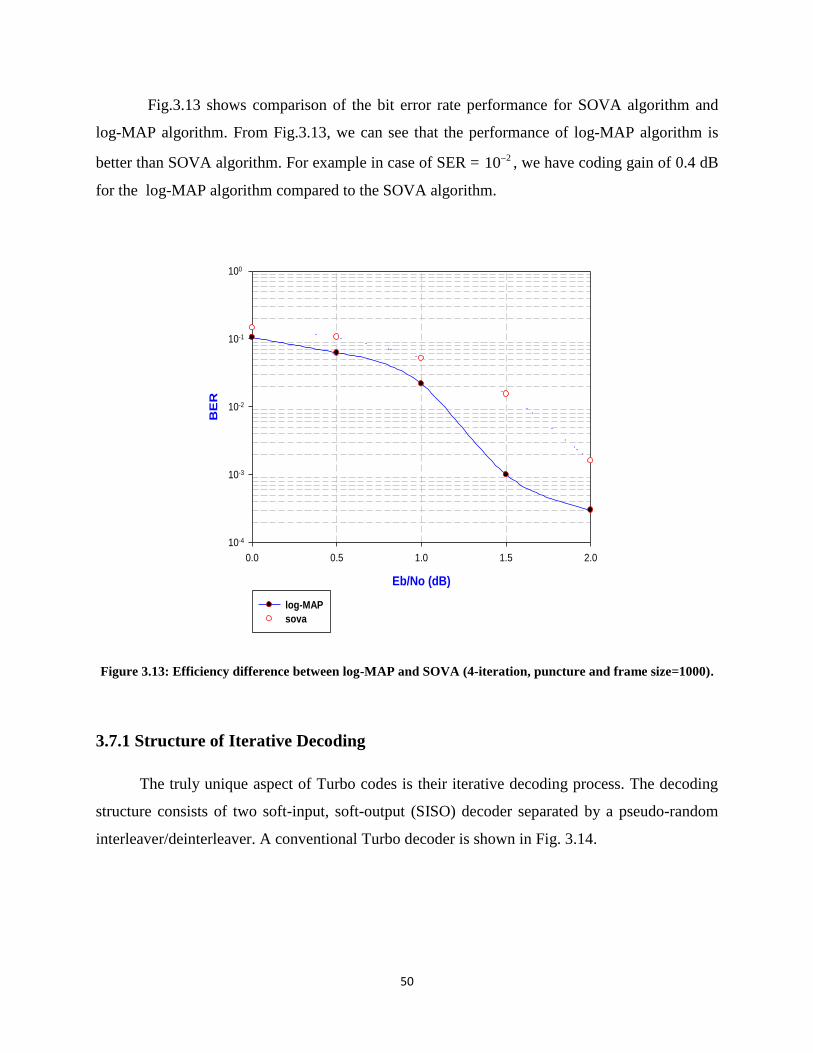
50
Fig.3.13 shows comparison of the bit error rate performance for SOVA algorithm and
log-MAP algorithm. From Fig.3.13, we can see that the performance of log-MAP algorithm is
better than SOVA algorithm. For example in case of SER = 210 , we have coding gain of 0.4 dB
for the log-MAP algorithm compared to the SOVA algorithm.
Eb/No (dB)
0.0 0.5 1.0 1.5 2.0
BE
R
10-4
10-3
10-2
10-1
100
log-MAP
sova
Figure 3.13: Efficiency difference between log-MAP and SOVA (4-iteration, puncture and frame size=1000).
3.7.1 Structure of Iterative Decoding
The truly unique aspect of Turbo codes is their iterative decoding process. The decoding
structure consists of two soft-input, soft-output (SISO) decoder separated by a pseudo-random
interleaver/deinterleaver. A conventional Turbo decoder is shown in Fig. 3.14.

51
Figure 3.14: Conventional Turbo decoder [32].
The first decoder operates on the systematic bits observation,(0)
ky , the parity bits
observation from the first RSC encoder, (1)
ky , and the a priori information bits, (1)
kz . The a priori
information bits for first decoder are initially set to all zeros. Both channel observations are
multiplied by the channel reliability s
o
4aENcL = . The variable a is the fading amplitude, and s
o
EN is
the SNR, where Es is the average symbol energy, and N0 is the noise power spectral density. In
high SNR and no fading case the channel reliability places more emphasis on the systematic and
parity bits observation. Likewise, more emphasis is placed on the a priori information kz when
the SNR is poor or when there is a deep fade. The channel reliability must be estimated in
practice, and correct estimation is essential for good Turbo code performance [25] [26]. The
output of the decoders is expressed as a log-likelihood ratio (LLR). A decoders output at time k
can be broken down into three distinct parts: the scaled systematic channel estimate(0)4( ).s
o
aEN ky ,
the a priori information kz , and the extrinsic information kl . The thk LLR is expressed as
4aE (0)sΛ = ( ).y + z + lNk k k ko . (3.1)
The extrinsic information is the new information generated by the current decoding
operation. In a Turbo decoder, the extrinsic information for the first decoder is determined by
subtracting the systematic channel observation and the current stage’s a priori information from
the LLR(1)
kΛ .The extrinsic information is then permuted by pseudo-random interleaver and used
as the weighted a priori information for the second decoding module. The second decoding

52
module operates on the weighted a priori information(2)
kz , the permuted channel observation(0)
ky ,
and the parity channel observation from the second RSC encoder(2)
ky to generate a new LLR,
(2)
kΛ , this completes one decoding iteration. If more decoding iterations are required, the extrinsic
information from second decoder is calculated by subtracting the permuted systematic channel
observation (0)
ky and the a priori information (2)
kz from the LLR(2)
kΛ . The extrinsic information is
then de-interleaved and used as the a priori information (1)
kz for the first decoding module in the
next decoding iteration. If all the decoding iterations have been completed, the final output (2)
kΛ
is de-interleaved and hard-limited to produce the final decision.[32]
3.7.2 Decoding Algorithms
Two classes of algorithms which are typically used to decode Turbo codes Fig 3.15. The
Viterbi algorithm (VA) accepts soft inputs with producing hard outputs. MAP algorithm accepts
soft inputs with producing soft outputs. Their derivatives, which are shown below the dotted line,
accept soft inputs and produce soft outputs. SISO algorithms are necessary for Turbo decoding
because the decoders are required to share their extrinsic information with each other. Although
SISO decoding algorithms are more computationally complex, they allow iterative sharing of
results between decoders, which permits the use of powerful concatenated coding structures.

53
Figure 3.15: Trellis-based decoding algorithms [32].
SOVA
In 1967 the Viterbe Algorithm (VA) was presented in [27] as a practical procedure for
maximum-likelihood decoding of convolutional codes. The VA minimizes error rate by finding
the most likely, connected path through the trellis. The VA is unsuitable for Turbo decoding
because it is a soft-input, hard-output algorithm. In [28], Hagenauer and Hoeher introduced a
soft-output VA (SOVA).It is a SISO algorithm, which retains information, related to the pruned,
competing paths. It determines the reliability of the bits which differ from those in the other path
(surviving path). Although it complexity is higher than the standard VA, the gains realized from
the soft-output decisions more than compensate for the additional complexity.
MAP
Based on an algorithm developed by Chang and Hancock for removing inter-symbol
interference, the MAP algorithm was introduced in 1974 as an optimal means for estimating the

54
a posteriori probabilities (APPs) [29]. The MAP algorithm, also known as the BCJR, algorithm
used a forward-backwards recursion algorithm which minimizes the probability of bit error.
Therefore, the path that the MAP algorithm traces through the trellis need not be
connected, as VA. In the 1970’s the MAP algorithm excluded from decoding convolutional
codes because it was less stable and more complex than the VA. When SISO decoding of Turbo
codes became an important issue, the Max-Log-MAP and Log-MAP algorithms were introduced
to solve the instability problem; they are now the preferred SISO algorithms used to decode
Turbo codes. The MAP algorithm calculates the APPs for each code symbol produced by a
Markov process given a noisy channel observation y. The APPs are kp[d = 1\ y] and
kp[d = 0\ y] . kp[d = 1\ y] is the probability that the information bit is a 1 given the received
vector y while kp[d = 0\ y] is the probability that the information bit is a 0 given the received
vector y. Once these probabilities are found, they are put into log-likelihood ratio (LLR) form in
order to make a decision on a particular symbol. The general form of the LLR for the thk bit is
[ ]= ln
[ ]
kk
k
P d = 1 / yΛ
P d = 0 / y. (3.2)
The MAP algorithm calculates the APPs by first finding the state transitional probability
[ ]k k+1P s s / y given the received signal y. The term ks represents the state of the encoder at
time k, and k k+1s s is the state transition from state ks to state 1ks at time k + 1. This
transitional probability is zero if state ks is not connected to state 1ks . Using Bayes ‟Law and
simplifying, the probability can be expressed as:
[ ][ ] =
[ ]
k k+1k k+1
P s s , yP s s / y
P y. (3.3)
The denominator in the expression above does not need to be explicitly calculated because
it will be canceled when the APPs are placed in LLR form. For notational convenience we define
k k+1 k k k+1 k k+1 k+1 k+1P[s s , y] = α (s ).γ (s s ).β (s ) , (3.4)

55
where k kα (s ) , k+1 k k+1γ (s s ) , and k+1 k+1β (s ) are defined in the following discussion. The term
k+1 k k+1γ (s s ) is the branch metric associated with the state transition k k+1s s . The branch
metric, which can be calculated from known information, is expressed as
= [ ]. [ ]
= [ ]. [ ].
k+1 k k+1 k+1 k k k k+1
k k k
γ (s s , y) P s \ s P y \ s s
P d P y \ x (3.5)
The probability [ ]kp d is derived from the a priori information, and the
probability [ ]k kp y \ x is determined from the received signal and knowledge of the trellis
structure. The probability k kα (s ) is equal to the probability [ ]k 1 2 kp s ,(y ,y ,…,y ) and can be found
by the forward recursion
k k k-1 k-1 k k-1 ksk-1
α (s ) = α (s ).γ (s s ) . (3.6)
Similarly, k kβ (s ) is equal to [ ]k+1 k+2 L-1 kp (y ,y ,…,y )\ s and can be found by the backward
Recursion
=k k k+1 k+1 k+1 k k+1sk+1
β (s ) β (s ).γ (s s )→ . (3.7)
When k kα (s )and ( )k ks have been found for all states along the trellis, the APPs for each state
transition are known. The APPs are related to the state transitional probabilities as:
[ ] = [ ]k k k+1si
P d = i \ y P s s \ y , (3.8)
where i {0,1} and si denotes the set of all state transitions associated with a message bit equal
to i. The LLR for the thk symbol can then be calculated as:
= ln
s k k k+1 k k+1 k+1 k+11k
s k k k+1 k k+1 k+1 k+10
α (s ).γ (s s ).β (s )Λ
α (s ).γ (s s ).β (s ). (3.9)

56
If the LLR kΛ is greater than zero, a binary ”1” is chosen as the most likely transmitted
symbol; conversely, if the LLR kΛ is less than zero, a binary ”0”is chosen. Because the
initialization of α and β is similar for the MAP, Max-Log-MAP, and Log-MAP algorithms, this
process will be explained in more detail in the following section.
Max-Log-MAP and Log-MAP
As mentioned previously, the MAP algorithm suffers from two serious drawbacks: its
computational complexity and its numerical instability. The solution to these problems is to
operate in the log-domain. One advantage of operating in the log-domain is that multiplication
becomes addition [31].
ln( ) = max( ) + ( )yx
e + e x, y f y - xc , (3.10)
where-x
cf (x)= ln(1+e ) . Addition is simply a maximization function plus a correction term in
the log-domain. The sub-optimal Max-Log-MAP algorithm approximates addition solely as
maximization. This is a reasonable approximation, especially when x and y are dissimilar. The
performance of the Log-MAP algorithm, however, is equivalent to the MAP algorithm. The Log-
MAP algorithm implements addition exactly as both the maximization function and the
correction term. For practical implementations, this correction function can be stored in a lookup
table. An 8-input lookup table in [30] was shown to give good performance in practice. Other
approximations exist, and the Turbo-coded system described in this thesis uses a linear
approximation developed in [16]. In the log-domain the branch metric k+1 k k+1γ (s s ) becomes
= ln = ln [ ]+ ln [ ]k+1 k k+1 k+1 k k+1 k k kγ (s ,s ) γ (s s ) P d P y \ x . (3.11)
Similarly, the probability k kα (s ) in the log-domain becomes
*
= ln = ln exp(
= max [ ],
k-1 A
k-1 A
k k k k k-1 k-1 k k-1 k
s
k-1 k-1 k k-1 ks
α (s ) α (s ) α (s )+ γ (s s ))
α (s )+ γ (s s )
(3.12)

57
where the *max (.) operation is equivalent to max(x, y) for the Max-Log-MAP algorithm and to
*max c(x, y)+ f ( y - x ) for the Log-MAP algorithm. Notice that the *max (.) operation is taken
over A, the set of all states k-1s which are connected to state ks . Likewise, k kβ (s )becomes
*
= ln = ln exp( ( ) + ( ))
= max [ ( ) + ( )]
k+1 B
k+1 B
k k k k k+1 k+1 k+1 k k+1
s
k+1 k+1 k+1 k k+1s
β (s ) β (s ) β s γ s s
β s γ s s
(3.13)
Here the *max (.) operation is taken over B, the set of all states k+1s which are connected to
state ks . After k kα (s )and k kβ (s ) are found for all states along the trellis, the LLRs are calculated
as
*
*
= max [ ]
- max [ ]
1
0
k k k k+1 k k+1 k+1 k+1s
k k k+1 k k+1 k+1 k+1s
Λ α (s )+ γ (s s )+ β (s )
α (s )+ γ (s s )+ β (s )
→→
(3.14)
1s is the set of all state transitions associated with an information bit kd = 1 , and 0s is the set of
all state transitions associated with an information bit kd = 0 . The Max-Log-MAP and the Log-
MAP algorithms are initialized in a manner analogous to the MAP algorithm. For a frame size N,
assume each constituent encoder starts in the all-zeros state. Then for time k = 0, the forward
path metric k is initialized as
0 and - for 00 0,0 0 j,0α (s ) = α (s ) = j (3.15)
For time k = N, the backwards path metric N is initialized in one of two ways. If the
encoder trellis is terminated, the backwards path metric is initialized as
0 and - for 0N 0,N N j,Nβ (s ) = β (s ) = j (3.16)
If the trellis is not terminated, then all states are equally likely to be the ending state.
Therefore, the backwards path metric is initialized as

58
for allN j,Nβ (s ) = 0 j (3.17)
3.8 Conclusion
In this chapter, the structure of both of encoder and decoder of Convolutional and Turbo coding
scheme are reviewed. Also, the operation of how the encoding and decoding of Turbo coding is
conducted. The types of Convolutional codes and Turbo-codes were presented with some
performance examples. The effects of the interleavers and punctured also are presented.

59
References
[1] C. Berrou and A. Glavieux, “Near optimum error correction coding and decoding: Turbo-
codes,” IEEE Transactions on Communications, vol. 44, pp. 1261–1271, Oct. 1996.
[2] P. Elias, “Coding for noisy channels,” I.R.E. Convention Record, pp.37-46, 1955.
[3] E. R. Berlekamp, Ed., “Key papers in the development of coding theory,” IEEE Press
Selected Reprint Series, New York: Institute of Electrical and Electronics Engineers, 1974.
[4] S. Lin and D. J. Costello, Jr., Error control coding: fundamentals and applications, Prentice-
Hall, 1983.
[5] R. Johannesson and K. Sh. Zigangirov, Fundamentals of convolutional coding, IEEE Press,
Piscataway, N.J., February, 1999.
[6] J. M. Wozencraft, “Sequential decoding for reliable communication,” Proc. IRE Convention
Record, pp. 2.11–25, 1957.
[7] R. M. Fano, “A heuristic discussion of probabilistic decoding,” IEEE Transactions
Information Theory, Vol. 9, pp. 64–74, April 1963.
[8] K. Sh. Zigangirov, “Some sequential decoding procedures,” Problemy Peredachi
Informatsii,Vol. 2, Iss. 4, P. 13–25, 1966.
[9] A. J. Viterbi, “Error bounds for convolutional codes and an asymptotically optimal decoding
algorithm,” IEEE Transactions Information Theory, Vol. 13, pp. 260–269, April 1967.
[10] G. D. Forney, Jr., “The Viterbi algorithm,” Proceedings of the IEEE, 61, PP. 268–278,
March 1973.
[11] G. D. Forney, Jr., “Convolutional codes II: maximum likelihood decoding,” Information
Control, 25, pp. 222–266, July 1974.
[12] L. R. Bahl, J. Cocke, F. Jelinek, and J. Raviv, “Optimal decoding of linear codes for
minimizing symbol error rate,” IEEE Transactions Information Theory, Vol. 20, 248–287, March
1974.
60
[13] C. Berrou, A. Glavieux, and P. Thitimajshima, “Near Shannon limit error correcting coding
and decoding: Turbo-codes,” Proceedings International Conference on Communications, pp.
1064–1070, May 1993.
[14] S. Benedetto, D. Divsalar, G. Montorsi, and F. Pollara, "A soft-input soft-output APP
module for the iterative decoding of concatenated codes," IEEE Communications Letters, vol. 1,
pp.22 -24, 1997.
[15] G. D. Forney, Concatenated Codes, Cambridge, MA: MIT Press, 1966.
[16] Y. Wu, “Implementation of parallel and serial concatenated codes,” PhD dissertation,
Virginia Polytechnic Institute and State University, April 2000.
[17] Sadjadpour, H., Sloane, N., Salehi, M., and Nebe, G., “Interleaver design for Turbo codes,”
IEEE J. Select. Areas Commun., vol. 19, pp. 831-837, May 2001.
[18] Hokfelt, J., Edfors, O., and Maseng, T., “Turbo codes: correlated extrinsic information and
its impact on iterative decoding performance,” in 1999 IEEE 49th Vehicular Technology
Conference, pp. 1871-1875, July 1999.
[19] M.A. Kousa and A.H. Mugaibel, “Puncturing effects on Turbo codes,” IEEE Proceedings
on Communications, Vol.149, pp.132-138, 2002
[20] Chatzigeorgiou, M. R. D. Rodrigues, I. J. Wassell and R. Carrasco,” Punctured binary
Turbo-codes with optimized performance,” EPSRC under Grant GR/S46437/01.
[21] J. Hagenauer and P. Hoher, “A Viterbi algorithm with soft outputs and its applications,”
Proceedings IEEE of the Global Communications Conference, 89, pp. 1680-1686, November
1989, Dallas, USA.
[22] J. P. Woodard and L. Hanzo, “Comparative study of Turbo decoding techniques: An
overview,” IEEE Transaction on Vehicular Technology, Vol. 49, No. 6, pp. 2208-2233,
November 2000.
[23] P. Robertson, E. Villebrun, and P. Hoher, “A comparison of optimal and sub-optimal MAP
decoding algorithms operating in the log domain,” Proceedings IEEE of International
Conference on Communication, 95, pp. 1009-1013, June 1995.

61
[24] C. Chaikalis and J. M. Noras, ”Implementation of an improved reconfigurable SOVA/log-
MAP Turbo decoder in 3GPP,” IEE Proceedings 3G2002, May 2002, London, UK
[25] M. A. Jordan and R. Nichols, “The effects of channel characteristics on Turbo code
performance,” Proceedings of the IEEE, MILCOM, pp. 17–21, 1996.
[26] T. A. Summers and S. G. Wilson, “SNR mismatch and online estimation in Turbo
decoding,” IEEE Transactions on Communications, vol. 46, pp. 421–423, Apr. 1998.
[27] A. J. Viterbi, “Error bounds for convolutional codes and an assymptotically optimum
decoding algorithm,” IEEE Transactions on Information Theory, vol. 13, pp. 260–269, Apr.
1967.
[28] J. Hagenauer and P. Hoeher, “A viterbi algorithm with soft-decision outputs and its
applications,” Proceedings of the IEEE, GLOBECOM, pp. 1680–1686, 1989.
[29] L. R. Bahl, J. Cocke, F. Jelinek, and J. Raviv, “Optimal decoding of linear codes for
minimizing symbol error rate,” IEEE Transactions on Information Theory, vol. 20, pp. 284–
287, Marsh 1974.
[30] P. Robertson, P. Hoeher, and E. Villebrun, “Optimal and sub-optimal maximum a
posteriori algorithms suitable for Turbo decoding,” European Transactions on
Telecommunications, vol. 8, pp. 119–125, Mar./April 1997.
[31] P. Ituero, P. Echeverria, M. Vallejo and C. Barrio, “Implementation trade-offs of the
Jacobian logarithm for several hardware platforms,” ETSI Telecommunication, 28040 Madrid,
Spain
[32] W. B. Puckett, “Implementation and performance of an improved Turbo decoder on a
configurable computing machine,” Thesis submitted to the Faculty of the Virginia Polytechnic
Institute and State University in Partial Fulfillment of The Requirements for The Degree of
Masters of Science in Electrical and Computer Engineering, July 7, 2000.
[33] P.B. harlesworth, “Turbo Codes,” 2000,site:http://www.philsrockets.org.uk/Turbocodes.pdf

62
Chapter 4
Uncoded and Turbo Coded
V-BLAST Architectures
4.1 Introduction
Today's wireless communication systems require high data rates and low bit error rates.
This motivated researchers to develop a new communication scheme called MIMO system.
MIMO system uses multiple antennas at the transmitter and/or the receiver to improve the error
performance. BLAST (Bell Labs Layered Space-Time) is a MIMO communication scheme,
which allows multiple symbols to be transmitted at the same time within the same frequency. So,
by using BLAST architecture high data rate can be achieved [4].
Moreover, in a high mobility environment, wireless channels become very unreliable. The
transmitted signal waves may hit unpredictably various objects and can be rejected and refracted
by those objects. This characteristic is known as multipath fading. In conventional wireless
systems, multipath is regarded as a serious impairment, because it results in multiple copies of
the transmitted symbol arriving at the receiver via different scattered paths. Those copies can
interfere destructively. In BLAST architecture, these scattering characteristics enhance
transmission accuracy by considering multiple scattering paths as separate parallel sub-channels.
This thesis focuses on two BLAST algorithms, namely the uncoded V-BLAST and the
coded V-BLAST using Turbo code.

63
In 1996, G.J Foschini proposed a diagonal-layer architecture for MIMO communication
system [1], which is known as D-BLAST (Diagonal BLAST). Due to the complexity of
implementation of the D-BLAST architecture, a modified version was proposed, which is known
as V-BLAST [2], [3].The performance of using Turbo code with V-BLAST architecture is a key
element on this thesis.
In this chapter the basic elements of a transmission and receiving scheme for uncoded-
BLAST and coded-BLAST architectures was introduced, several issues of using Turbo code
with V-BLAST MIMO system was discussed, the difference between uncoded V-BLAST
system and V-BLAST system using Turbo code is discussed, the effects of using different types
of detection with coded V-BLAST system is also presented , Moreover, using a new detection
type V-BLAST/MAP “which combines features of MAP and V-BLAST rules and uses the
layered structure of V-BLAST, by using a different strategy for channel processing order,
inspired by the MAP rule” with coded V-BLAST system is also introduced and compares its
performance with different detection algorithms.
4.2 Uncoded V-BLAST System
4.2.1 Uncoded V-BLAST Transmitter
Figure 4.1 shows the transmitter of uncoded V-BLAST system with M transmitting
antennas. The bit stream b is demultiplexed into M sub-streams 1 2, ,...,b b and Mb .The 1 2, ,...,b b
and Mb are mapped to complex symbols 1 2, , ...,s s and Ms are transmitted from 1 2, , ...,TX TX
and MTX , respectively. V-BLAST algorithm uses a layered structure. The layering is horizontal
as all the symbols of a certain stream are transmitted through the same antenna. Fig. 4.2 shows
the V-BLAST process at the transmitter. It shows the antenna and time instant for the symbol to
be transmitted. This process is shown with 4 transmitting antennas. After demultiplexing and
modulation of bit stream b, the symbol vectors transmitted from modulator 1, 2, 3 and 4 are
denoted as 1 2 3, ,s s s and 4s , respectively. Now s1 can be expressed as 13 14[ ]11 12s ,s ,s ,s .
Similarly 2s , 3s and 4s can be expressed as 23 24[ ]21 22s ,s ,s ,s , 33 34[ ]31 32s ,s ,s ,s and 43 44[ ]41 42s ,s ,s ,s .

64
Figure4.1: Uncoded V-BLAST Transmitter.
Figure 4.2: Uncoded V-BLAST Vectors at Transmitter.
Now at a time instant 1t , the symbol 11s from modulator 1 is transmitted from antenna 1, the
symbol 21s from modulator 2 is transmitted from antenna 2, the symbol 31s from modulator 3 is
transmitted from antenna 3, and the symbol 41s from modulator 4 is transmitted from antenna 4.
Similarly in next time instant 2t , the symbols 1311 12s ,s ,s and 14s from modulators 1, 2, 3, and 4 are

65
transmitted from antenna 1, 2, 3, and 4, respectively. Therefore the symbol vector 1s is
transmitted from antenna 1 only, the symbol vector 2s is transmitted from antenna 2, and so on.
4.2.2 Uncoded V-BLAST Receiver
In the transmitter part, streams are independently transmitted; we need to separate the M
transmitted streams and then demodulated them separately with the demodulators.
Figure 4.3: Uncoded V-BLAST Receiver.
Figure 4.3 shows the basic block diagram of uncoded V-BLAST receiver with N receiving
antennas. In the receiver section, one of the V-BLAST detectors ”ZF, LLSE or MAP is used. A
detailed explanation for these detectors can be found in Chapter 2 of this thesis”. The input of the
detector is the received victor 1 2, ,...r r and Nr , and the output is an estimation of transmitted
symbols denoted by' '
1 2, ,...s s and '
Ms . The estimated symbol vector is demodulated and
multiplexed to recover transmitted data bits.
In the detection process, there are three steps [4]:
[1] Interference nulling: at one instant, one sub-stream is regarded as desired symbols and
others sub-streams are interferers. At the next instant, another sub-stream will be regarded as

66
desired symbols and other sub-streams are interferers. In each detection step undesired
symbols are nulled by multiplying the received vector with nulling vectors.
[2] Interference cancellation: In interference cancellation step, interference from already
detected components is subtracted out from the received vector. From that a modified
received vector r new is obtained where fewer interferers are present.
[3] Optimal ordering (optional): For V-BLAST detection, optimal ordering is done for
better performance. When symbol cancellation is used, the order in which the streams of
received vector r are detected becomes important. The performance will be better if the
interference from strong symbols i.e. having high signal to noise ratio is removed earlier. So
it is required to determine a particular ordering which is optimal in a certain sense. A simple
optimal ordering is based on the post detection SNR of each sub-stream. The SNR for thi sub-
stream is proportional to the norm of the column i of the channel matrix, H. Thus the optimal
detection order is in decreasing order of the second norm of the columns of H.
4.3 Coded V-BLAST MIMO System
4.3.1 Coded V-BLAST MIMO Transmitter
Figure 4.4 shows the basic block diagram of coded V-BLAST transmitter with M
transmitting antennas. The bit stream b is demultiplexed into M sub-streams 1 2, ,...b b and Mb , and
each sub-stream is coded separately by ½ -rate Turbo code which consists of two convolutional
encoders. Each sub-stream bits 11 12 13 14 21 22 23 24( , , , ),( , , , ),...b b b b b b b b and 1 2 3 4( , , , )M M M Mb b b b enter
to the first encoder in each Turbo encoder and the same bits inter to the second encoder after it
has been interleaved. The output of the Turbo encoder is given by
11 12 13 14 11 12 13 14 21 22 23 24 21 22 23 24( , , , , , , , ),( , , , , , , , )c c c c cp cp cp cp c c c c cp cp cp cp ,... and 1 2( , ,M Mc c
3 4 1 2 3 4, , , , , )M M M M M Mc c cp cp cp cp , consists of the systematic bits C of the first encoder, the parity
bits CP “which are punctured using puncturing vector, based on pattern Pp = [1,0]”of the first
encoder and the parity bits of the second encoder “ which are punctured using puncturing vector,
based on pattern Pp'=[0,1]”. The 1 2, ,...c c and Mc bits are interleaved using pseudo-random
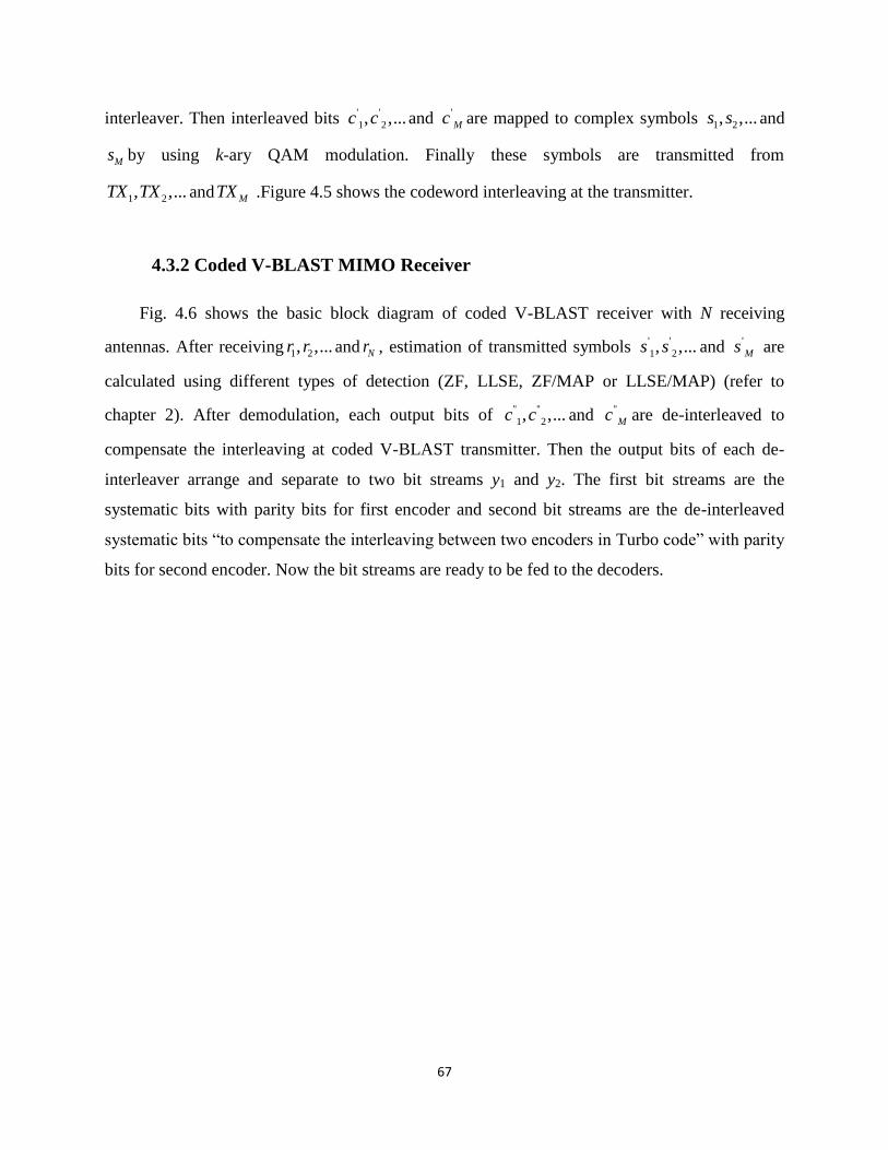
67
interleaver. Then interleaved bits ' '
1 2, ,...c c and '
Mc are mapped to complex symbols 1 2, ,...s s and
Ms by using k-ary QAM modulation. Finally these symbols are transmitted from
1 2, ,...TX TX and MTX .Figure 4.5 shows the codeword interleaving at the transmitter.
4.3.2 Coded V-BLAST MIMO Receiver
Fig. 4.6 shows the basic block diagram of coded V-BLAST receiver with N receiving
antennas. After receiving 1 2, ,...r r and Nr , estimation of transmitted symbols ' '
1 2, ,...s s and '
Ms are
calculated using different types of detection (ZF, LLSE, ZF/MAP or LLSE/MAP) (refer to
chapter 2). After demodulation, each output bits of '' ''
1 2, ,...c c and ''
Mc are de-interleaved to
compensate the interleaving at coded V-BLAST transmitter. Then the output bits of each de-
interleaver arrange and separate to two bit streams y1 and y2. The first bit streams are the
systematic bits with parity bits for first encoder and second bit streams are the de-interleaved
systematic bits “to compensate the interleaving between two encoders in Turbo code” with parity
bits for second encoder. Now the bit streams are ready to be fed to the decoders.
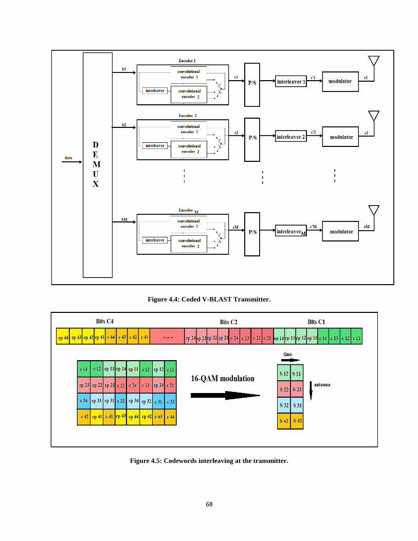
68
Figure 4.4: Coded V-BLAST Transmitter.
Figure 4.5: Codewords interleaving at the transmitter.

69
Figure 4.6: Coded V-BLAST Receiver.
The first decoder operates on the systematic channel observation,(0)
1y , the parity channel
observation from the first RSC encoder,(1)
1y , and the a priori information from second decoder,
1z . In first iteration the a priori information is initially set to all zeros. This implies that each
information bit is equally likely to be a 0 or a 1 initially. The output of decoders is expressed as a
log-likelihood ratio (LLR). A decoders output at time k can be broken down into three distinct
parts: the systematic channel estimate, the a priori information kz , and the extrinsic
information kl . The thk LLR is expressed as
Λ = y + z + lk k k k
(4.1)

70
The extrinsic information is the new information generated by the current decoding
operation. In a Turbo decoder, the extrinsic information for the first decoder is determined by
subtracting the systematic channel observation and the current stage’s a priori information from
the LLR 1Λ . The extrinsic information is then permuted by pseudo-random interleaver and used
as the weighted a priori information for the second decoding module. The second decoding
module operates on the weighted a priori information 2z , the permuted systematic channel
observation 2
(0)y , and the parity channel observation from the second RSC encoder 2
(1)y to generate
a new LLR, 2Λ ; this completes one decoding iteration. If more decoding iterations are required,
the extrinsic information from second decoder is calculated by subtracting the permuted
systematic channel observation 2
(0)y and the a priori information 2z from the LLR 2Λ . The
extrinsic information is then de-interleaved and used as the a priori information 1z for the first
decoding module in the next decoding iteration. If all the decoding iterations have been
completed, the final output 2Λ is de-interleaved and hard-limited to produce the final decision
[5].
4.4 Simulation Results
In this thesis, all the simulations were done in MATLAB 2011a. The performance of the
system has been simulated for different value of the signal-to-noise-ratio (SNR). The schemes
under investigation are the BLAST scheme (uncoded V-BLAST and coded V-BLAST using
Turbo code). While, the detection strategies used in this thesis are (zero-forcing, LLSE, V-
BLAST/ ZF, V-BLAST/LLSE, V-BLAST/ZF/MAP, V-BLAST/LLSE/MAP,V-BLAST/ZF/
ordering or V-BLAST/LLSE/ordering). We have also considered in our simulation different
frame lengths, and different number of iterations for Turbo decoder. The channel encoder is 1/2
rate Turbo encoder which has two puncturing 4-state Convolutional encoders “which have been
punctured with pattern in the Table 4.2” with generators polynomial (7,5) octal, see Fig. 4.7.
Table 4.1 shows a 1/2 rate convolution code used in this thesis. The type of channel decoder is
LOG-MAP-Decoder which discussed in chapter 3 and type of modulation is 16 QAM. The
results in [6] are taken as reference.

71
Memory size Generator polynomial in octal Generator polynomial in binary
2 [7,5] [111,101]
Table 4.1. The parameters of a 1/2 rate convolution code.
Puncturing patterns
Systematic output of the first encoder [1 1] Parity output of the first encoder [1 0] Parity output of the second encoder [0 1]
Table 4.2: Puncturing patterns
Figure 4.7: Illustration of how the generator polynomials determined.
The channel is Rayleigh fading with Additional White Gaussian noise (AWGN). For each
frame, a new random realization of the channel matrix H is used. There are 10000 frames and
each frame has 16 bits. A frame is considered to be received incorrectly if any single bit of a
frame is wrongly decoded.
4.4.1 Performance Analysis
In this section, the performance of coded V-BLAST using Turbo code and uncoded V-
BLAST with different types of detection strategies is investigated. To enhance the performance
of the system, we have considered symbol ordering in V-BLAST. For coded V-BLAST, the

72
effect on symbol error rate performance for different number of Turbo iterations is also
investigated.
Figures 4.8 show comparison of the symbol error rate performance for different frame size
of Turbo/ normal LLSE without interference nulling and interference cancellation.
Figures 4.9 and 4.10 shows comparison of the symbol error rate performance for coded V-
BLAST using Turbo code without ordering and with best order architectures using 44 MIMO
system and 16-QAM modulation. The detection is done by ZF and LLSE techniques.
From Figures 4.9 and 4.10, we can see that the performance of Turbo/V-BLAST/ZF with
best order architecture is better than Turbo/V-BLAST/ZF without order architecture. For
example in case of SER = 110 , we have coding gain of 3.3 dB for the ordered coded system
compared to the system without symbol ordering.
Whereas the gain in case of symbol ordering for Turbo code with LLSE detection technique is
5.3 dB at symbol error rate of 210 .
Figure 4.8: The SER performance for different frame size of Turbo/ normal LLSE.

73
Figure 4.9: The SER performance for coded V-BLAST/ZF using Turbo code and coded V-BLAST/ZF using
Turbo code with best order.
Figure 4.11 shows comparison of the symbol error rate performance for Turbo/normal ZF
without Interference nulling and Interference cancellation, Turbo/V-BLAST/ZF and proposed
Turbo/V-BLAST/ZF/MAP techniques with 4×4 antennas and 16-QAM modulation. The
detection is done by ZF technique.
From Figure 4.11, we can see that, the performance of Turbo/V-BLAST/ZF/MAP technique
is best among the three techniques. The performance of Turbo/V-BLAST/ZF is better than
Turbo/normal ZF without Interference nulling and Interference cancellation. For example in case
of SER = 110 , we have coding gain of 4 dB for the Turbo/V-BLAST/ZF system compared to
the Turbo/normal ZF system. Whereas the gain in case of Turbo/V-BLAST/ZF/MAP system is
1.6 dB compared to the Turbo/V-BLAST/ZF system at symbol error rate of 210 .

74
Figure 4.10: The SER performance for coded V-BLAST/MMSE using Turbo code and coded V-
BLAST/MMSE using Turbo code with best order.
Figure 4.12 shows comparison of the symbol error rate performance for Turbo/normal
LLSE without interference nulling and interference cancellation, Turbo/V-BLAST/LLSE and
proposed Turbo/V-BLAST/LLSE/MAP techniques with 4×4 antennas and 16-QAM modulation.
The detection is done by LLSE technique.
From figure 4.12, we can see that the performance of Turbo/V-BLAST/LLSE/MAP
technique is best among the three techniques. The performance of Turbo/V-BLAST/LLSE is
better than Turbo/normal LLSE without Interference nulling and Interference cancellation. For
example in case of SER = 210 , we have coding gain of 5 dB for the Turbo/V-BLAST/LLSE
system compared to the Turbo/normal LLSE system. Whereas the gain in case of Turbo/V-
BLAST/LLSE/MAP system is 1 dB compared to the Turbo/V-BLAST/LLSE system at symbol
error rate of 310 .

75
Figure 4.11: The SER performance for coded normal ZF, V-BLAST/ZF and V-BLAST/ZF/MAP using
Turbo.
Figure 4.13 shows comparison of the symbol error rate performance for VBLAST/ZF
without coding and V-BLAST/ZF coding with using Turbo code techniques with 4×4 antennas
and 16-QAM modulation. The detection is done by ZF technique.
From figure 4.13, we can see that the performance of coded V-BLAST/ZF is better than
uncoded V-BLAST/ZF. For example in case of SER = 110 , we have coding gain of 3.6 dB for
the system with Turbo code compared to uncoded VBLAST/ZF system .
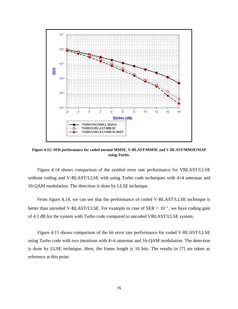
76
Figure 4.12: SER performance for coded normal MMSE, V-BLAST/MMSE and V-BLAST/MMSE/MAP
using Turbo.
Figure 4.14 shows comparison of the symbol error rate performance for VBLAST/LLSE
without coding and V-BLAST/LLSE with using Turbo code techniques with 4×4 antennas and
16-QAM modulation. The detection is done by LLSE technique.
From figure 4.14, we can see that the performance of coded V-BLAST/LLSE technique is
better than uncoded V-BLAST/LLSE. For example in case of SER = 210 , we have coding gain
of 4.3 dB for the system with Turbo code compared to uncoded VBLAST/LLSE system.
Figure 4.15 shows comparison of the bit error rate performance for coded V-BLAST/LLSE
using Turbo code with two iterations with 4×4 antennas and 16-QAM modulation. The detection
is done by LLSE technique. Here, the frame length is 16 bits. The results in [7] are taken as
reference at this point.

77
From figure 4.15, we can see that the performance of coded V-BLAST/LLSE technique at
second iteration of Turbo decoder is better than first iteration. For example in case of SER =
110 , we have coding gain of 1.8 dB for the second iteration compared to the first iteration .
Figure 4.13: SER performance for uncoded V-BLAST/ZF and coded V-BLAST/ZF using Turbo code.

78
Figure 4.14: SER performance for uncoded V-BLAST/MMSE and coded V-BLAST/MMSE using Turbo
code.
Figure 4.15: SER performance for coded V-BLAST/MMSE using Turbo code with two iterations.

79
4.5 Conclusion
In this chapter, performances of normal MIMO system using ZF and LLSE detection have
been done. Performances of different types of detection with coded V-BLAST using Turbo code
and uncoded V-BLAST architectures have also been tested. Performance of ZF/MAP and
LLSE/MAP detection with coded V-BLAST using Turbo code and uncoded V-BLAST
architectures have also been tested. All simulations have been developed using MATLAB
software. It has been shown that the performance of proposed coded V-BLAST architecture with
using LLSE/MAP detection provides the best performance in term of SER compared to all the
other configurations. The performance of coded V-BLAST architecture with using
VBLAST/LLSE can be improved by increasing the number of iterations. However, this iterative
process adds extra complexity to the system. The performance with LLSE detection is better than
ZF detection and the hence the performance with VBLAST/LLSE detection is better than
VBLAST/ZF detection.
Furthermore, the effect of ordering on V-BLAST detection has been presented in this
chapter. With ordering, the V-BLAST architecture works well.

80
References
[1] G. J. Foschini and M. J. Gans, “On limits of wireless communication in a fading environment
when using multiple antennas," Wireless Personal Communication, vol. 6, pp. 331-335, 1998.
[2] G. J. Foschini, “Layered space-time architecture for wireless communication in a fading
environment when using multi-element antennas," Bell Labs Technical Journal, pp.41-59,
Autumn 1996.
[3] G. J. Foschini, G. D. Golden, R. A. Velenzuela, and P. W. Wolniansky, “Simplified
processing for high spectral efficiency wireless communication employing multi-element
arrays," IEEE Journal on Selected Areas in Communication, vol. 17, no. 11, pp. 1841-1852,
November 2005.
[4] ApalaRay, “Performance of different BLAST architectures," A Thesis Submitted in Partial
Fulfillment for the Award of M.Tech in Information Technology, 2006-2012.
[5] W. Bruce Puckett, “Implementation and performance of an improved Turbo decoder on a
configurable computing machine," Faculty of the Virginia Polytechnic Institute and State
University, July 7, 2000.
[6] S. Jani, S. Yadav, B. L. Pal, “Analysis of various symbol detection techniques in multiple-
input multiple-output system (MIMO),” Advanced Computing: An International Journal (ACIJ),
vol.3, no.2, March 2012.
[7] D. Na, G. P. biao and C. Ning, “A low-complexity iterative receiver scheme for Turbo-
BLAST system,” ICSP2010 proceeding, 2010.

81
Chapter 5
Conclusions
5.1 Conclusion
In this thesis, a successful implementation of a new system design
“Turbo/VBLAST/MAP”, which combines Turbo code with newly emerged detection technique”
V-BLAST/MAP”. The block diagrams of V-BLAST system and Turbo/VBLAST system are
presented and described. A detailed description for encoding and decoding process of
Turbo/VBLAST is presented. The Turbo/V-BLAST system was presented with different
detection techniques.
Comparison between these schemes was made to observe that the LLSE algorithm performs
slightly better than ZF algorithm. Whereas, the same stands in case of using V-BLAST/LLSE is
perform better than V-BLAST/ZF and V-BLAST/LLSE/MAP is perform better than V-
BLAST/ZF/MAP. Using V-BLAST/MAP with either ZF or LLSE improve the performance of
the system significantly.
In addition, using an 44 MIMO system and 16-QAM modulation simulation comparison
between the coded and uncoded V-BLAST to observe that the performance of the coded V-
BLAST is better than uncoded V-BLAST, “there is a gain of 4.3 dB at 210
with LLSE and 3.6
dB at 110
with ZF”, comparison between the ordered Turbo/V-BLAST and unordered
Turbo/V-BLAST to observe that the performance of the ordered Turbo/V-BLAST is better than

82
unordered Turbo/V-BLAST, “there is a gain of 3.3 dB at 110
with ZF and 5.3 dB at 210
with
LLSE”, comparison between the different detection techniques of Turbo/V-BLAST/ZF to
observe that the performance of Turbo/V-BLAST/ZF/MAP technique is the best among
Turbo/V-BLAST/ZF and Turbo/normal ZF techniques, “there is a gain of 1.6 dB at 210
to the
Turbo/V-BLAST/ZF/MAP compare to Turbo/V-BLAST/ZF and 4 dB at 110
to the Turbo/V-
BLAST/ZF compare to Turbo/normal ZF and comparison between the different detection
techniques of Turbo/V-BLAST/LLSE to observe that the performance of Turbo/V-
BLAST/LLSE/MAP technique is the best among Turbo/V-BLAST/LLSE and Turbo/normal
LLSE techniques, “there is a gain of 1 dB at 310
to the Turbo/V-BLAST/LLSE/MAP compare
to Turbo/V-BLAST/LLSE and 5 dB at 210
to the Turbo/V-BLAST/LLSE compare to
Turbo/normal LLSE were made.
However, we may state as the main conclusion of this thesis that Turbo/V-BLAST/MAP
offers significantly better SER performance than others V-BLAST techniques at a modest
increase in complexity.
5.2 Future works:
Optimizing the parameters for Turbo codes such as interleaving size, puncturing pattern
and frame size.
Analyzing and proposing ideas to overcome the problem of noise floor “error floor” and
show its effect when it used with Turbo/V-BLAST/MAP.
Design a new decoding scheme based on increasing the number of iteration before the
detection.
Increase the number used of convolution encoders and show its effect when it used with
Turbo/V-BLAST/MAP.
Use different type of encoder instead of convolution encoder which used in Turbo encoder.
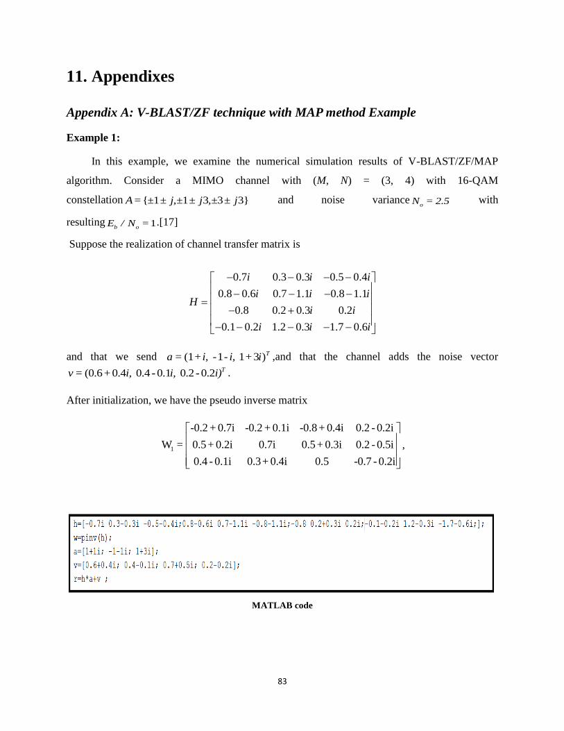
83
11. Appendixes
Appendix A: V-BLAST/ZF technique with MAP method Example
Example 1:
In this example, we examine the numerical simulation results of V-BLAST/ZF/MAP
algorithm. Consider a MIMO channel with (M, N) = (3, 4) with 16-QAM
constellation { 1 1 3 3 3}A= ± ± j,± ± j ,± ± j and noise varianceo
N = 2.5 with
resulting 1b o
E / N = .[17]
Suppose the realization of channel transfer matrix is
0.7 0.3 0.3 0.5 0.4
0.8 0.6 0.7 1.1 0.8 1.1
0.8 0.2 0.3 0.2
0.1 0.2 1.2 0.3 1.7 0.6
i i i
i i iH
i i
i i i
and that we send (1 1 1 3 )Ta = +i, - - i, + i ,and that the channel adds the noise vector
(0.6 + 0.4 0.4 - 0.1 0.2 - 0.2 Tv = i, i, i) .
After initialization, we have the pseudo inverse matrix
1
-0.2 + 0.7i -0.2 + 0.1i -0.8 + 0.4i 0.2 - 0.2i
W = 0.5+ 0.2i 0.7i 0.5+ 0.3i 0.2 - 0.5i
0.4 - 0.1i 0.3+ 0.4i 0.5 -0.7 - 0.2i
,
MATLAB code

84
Results in command window
We compute
1
-0.2 +1.1i
y = -0.6 - 0.1i
1.6 + 3.6i
,
and
1
-1.0 +1.0i
s = -1.0 -1.0i
1.0 + 3.0i
,
The reliability estimates are computed as

85
11
12
13
p = 0.546
p = 0.454
p = 0.785
Therefore, the algorithm sets 1k to 3 and the third component of the decision is chosen to be
1k 13a = s =1.0 + 3.0i
After symbol cancellation, we get the following modified received vector
1 12 1 k k
0.8 - 0.3i
0.6iˆr = r - a (H) =
-0.8i
-1.2 -1.3i
and new pseudo inverse 2W for next iteration is computed to be
2
-0.1+ 0.4i 0.3+ 0.1i -0.5+ 0.1i -0.3+ 0.1i
W = 0.1 0.1+ 0.3i 0.2 - 0.1i 0.4 + 0.1i
0 0 0 0
After calculation we get
2k 22a = s = -1.0 -1.0i and
3k 31a = s =1.0 +1.0i
We may combine the components of decision vector according to the order of indices 1 2 3(k ,k ,k ) ,
and obtain
1+ i
a = -1- i
1+ 3i
which is the correct estimate of a.

86
MATLAB code
The results in command window were:
r =
1.4000 - 2.2000i
2.5000 - 3.0000i
-0.6000 - 0.6000i
-1.1000 - 7.1000i
y =
-0.3136 + 1.1246i
-0.5628 - 0.0741i
1.6574 + 3.6060i

87
ahat =
-1.0000 + 1.0000i -1.0000 - 1.0000i 1.0000 + 3.0000i
p =
0.5742 0.4602 0.7578
Y =
0.7578
I =
3
zb1 =
0 0 1.0000 + 3.0000i
r =
0.7000 - 0.3000i
0 + 0.5000i
0 - 0.8000i
-1.2000 - 1.4000i
w =
-0.0691 + 0.3515i 0.2809 + 0.1526i -0.4848 + 0.0656i -0.3017 + 0.0982i
0.1302 - 0.0311i 0.1112 + 0.2411i 0.2263 - 0.0770i 0.4482 + 0.0699i
0 0 0 0
y =
0.5327 + 1.0997i
-0.5403 - 0.8977i
0
ahat =
1.0000 + 1.0000i -1.0000 - 1.0000i -1.0000 - 1.0000i
p =
0.9744 0.9978 -1.0000

88
Y =
0.9978
I =
2
zb1 =
0 -1.0000 - 1.0000i 1.0000 + 3.0000i
r =
1.3000 - 0.3000i
1.8000 + 0.1000i
-0.1000 - 0.3000i
0.3000 - 0.5000i
w =
0 + 0.3211i 0.3670 + 0.2752i -0.3670 - 0.0000i -0.0459 + 0.0917i
0 0 0 0
0 0 0 0
y =
0.7982 + 1.1101i
0
0
ahat =
1.0000 + 1.0000i -1.0000 - 1.0000i -1.0000 - 1.0000i
p =
0.9985 -1.0000 -1.0000
Y =
0.9985
I =
1

89
zb1 =
1.0000 + 1.0000i -1.0000 - 1.0000i 1.0000 + 3.0000i
r =
0.6000 + 0.4000i
0.4000 - 0.1000i
0.7000 + 0.5000i
0.2000 - 0.2000i
w =
0 0 0 0
0 0 0 0
0 0 0 0