Embed Size (px)
Citation preview
Sede Amministrativa: Università degli Studi di Padova
Centro di Ateneo di Studi ed Attività Spaziali "Giuseppe Colombo" (CISAS)
________________________________________________________________________________
CORSO DI DOTTORATO DI RICERCA IN: SCIENZE TECNOLOGIE E MISURE SPAZIALI
INDIRIZZO: MISURE MECCANICHE PER L'INGEGNERIA E LO SPAZIO
CICLO XXIX
DEVELOPMENT AND TESTING OF HARDWARE SIMULATOR FOR SATELLITE
PROXIMITY MANEUVERS AND FORMATION FLYING
Direttore del Corso: Ch.mo Prof. Giampiero Naletto
Coordinatore di Indirizzo: Ch.mo Prof. Stefano Debei
Supervisore: Ch.mo Prof. Enrico Lorenzini
Dottorando: Sergio Tronco

2
ABSTRACT
Satellite Formation Flying (SFF) and Proximity Operations are applications that have increasingly
gained interest over the years. These applications foresee the substitution of a single spacecraft with
a system of multiple satellites that perform coordinated position and attitude control maneuvers,
which in turn results in higher accuracy of payload measurement, higher flexibility, robustness to
failure, and reduction of development costs. These systems present however higher difficulties in
their design since they have not only absolute but also relative state requirements, which make them
also liable to higher control action expense with respect to (wrt) the single satellite systems.
Moreover, applications like Automated Rendez-Vous and Docking (RVD) and in general close
proximity maneuvers present a high risk of impact between the satellites, which must be treated
with an appropriate design of the on board Guidance Navigation and Control (GNC) system. These
aspects justify the development and employment of a ground hardware simulator representative of
two or more satellites performing coordinate maneuvers, allowing the investigation of these
problems with an easily accessible system.
The aim of my Ph.D. Activities has consisted in the development and testing of the cooperating
SPAcecRaft Testbed for Autonomous proximity operatioNs experimentS (SPARTANS) hardware
simulator, which is under development since 2010 at the Center of Studies and Activities for Space
(CISAS) of the University of Padova. This ground simulator presents robotic units that allow the
reproduction of the relative position and attitude motions of satellites in proximity or in formation,
and can be therefore employed for the extensive study of control algorithms and strategies for these
types of applications, allowing dedicated hardware in the loop to be tested in a controlled
environment. At the beginning of my Ph.D., the testbed consisted in the first prototype of Attitude
Module (AM), a platform with three rotational Degrees of Freedom (DOF) of Yaw, Pitch and Roll,
controllable through a GNC system based on incremental encoders and air thrusters. A small
contribution was initially given in support of the execution of a series of 3 DOF attitude control
maneuvers tests with the AM. Subsequently, the first activity consisted in the design and
development of the air suspension system that enables a low friction translational motion of the a
whole Unit of the testbed over the test table, with the characterization of air skids available in
laboratory. The subsequent activity consisted in the design and development of the Translation
Module (TM), the lower section of the whole Unit, as modular structure supporting the air
suspension system, the AM, and the on board localization system. After this activity the on board
localization system for position and Azimuth estimation, based on Optical Flow Sensors (OFS), was
developed and tested. The system was installed on a TM base prototype and it was calibrated and
3
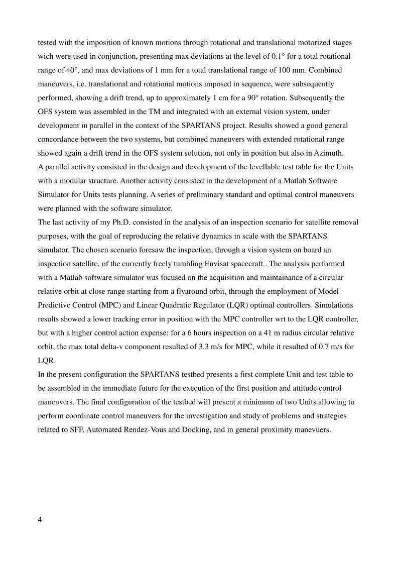
tested with the imposition of known motions through rotational and translational motorized stages
wich were used in conjunction, presenting max deviations at the level of 0.1° for a total rotational
range of 40°, and max deviations of 1 mm for a total translational range of 100 mm. Combined
maneuvers, i.e. translational and rotational motions imposed in sequence, were subsequently
performed, showing a drift trend, up to approximately 1 cm for a 90° rotation. Subsequently the
OFS system was assembled in the TM and integrated with an external vision system, under
development in parallel in the context of the SPARTANS project. Results showed a good general
concordance between the two systems, but combined maneuvers with extended rotational range
showed again a drift trend in the OFS system solution, not only in position but also in Azimuth.
A parallel activity consisted in the design and development of the levellable test table for the Units
with a modular structure. Another activity consisted in the development of a Matlab Software
Simulator for Units tests planning. A series of preliminary standard and optimal control maneuvers
were planned with the software simulator.
The last activity of my Ph.D. consisted in the analysis of an inspection scenario for satellite removal
purposes, with the goal of reproducing the relative dynamics in scale with the SPARTANS
simulator. The chosen scenario foresaw the inspection, through a vision system on board an
inspection satellite, of the currently freely tumbling Envisat spacecraft . The analysis performed
with a Matlab software simulator was focused on the acquisition and maintainance of a circular
relative orbit at close range starting from a flyaround orbit, through the employment of Model
Predictive Control (MPC) and Linear Quadratic Regulator (LQR) optimal controllers. Simulations
results showed a lower tracking error in position with the MPC controller wrt to the LQR controller,
but with a higher control action expense: for a 6 hours inspection on a 41 m radius circular relative
orbit, the max total delta-v component resulted of 3.3 m/s for MPC, while it resulted of 0.7 m/s for
LQR.
In the present configuration the SPARTANS testbed presents a first complete Unit and test table to
be assembled in the immediate future for the execution of the first position and attitude control
maneuvers. The final configuration of the testbed will present a minimum of two Units allowing to
perform coordinate control maneuvers for the investigation and study of problems and strategies
related to SFF, Automated Rendez-Vous and Docking, and in general proximity manevuers.
4

5
SOMMARIO
Il volo in formazione e le manovre di prossimità tra satelliti sono applicazioni che hanno
progressivamente acquisito interesse negli ultimi anni. Queste applicazioni prevedono la
sostituzione di un singolo satellite con sistemi formati da più satelliti che eseguono manovre
coordinate di controllo di posizione e assetto, il che comporta un aumento di accuratezza delle
misure dei payload distribuiti, maggior flessibilità, robustezza alle avarie, e riduzione dei costi di
sviluppo. Ciònonostante questi sistemi presentano difficoltà maggiori nella loro progettazione, in
quanto hanno requisiti di stato non solo assoluti ma anche relativi, il che li rende anche portati a
maggiore spesa di azione di controllo rispetto ai sistemi satellitari singoli. Inoltre applicazioni come
Automated Rendez-Vous and Docking (RVD) ed in generale manovre di prossimità presentano un
alto rischio di impatto tra satelliti, che va trattato con una progettazione appropriata del sistema di
Guida Navigazione e Controllo (GNC) di bordo. Questi aspetti giustificano lo sviluppo e l'utilizzo
di un simulatore hardware a terra, rappresentativo di due o più satelliti che eseguono manovre
coordinate, permettendo l'investigazione e lo studio di queste problematiche con un sistema
facilmente accessibile.
Lo scopo delle mie attività di dottorato è consistito nello sviluppo e collaudo del simulatore
hardware cooperating SPAcecRaft Testbed for Autonomous proximity operatioNs experimentS
(SPARTANS), in sviluppo dal 2010 presso il Centro di Ateneo di Studi e Attività Spaziali (CISAS)
dell'Università degli Padova. Questo simulatore di terra presenta Unità robotiche che permettono la
riproduzione dei moti relativi di assetto e posizione di satelliti in formazione o in prossimità, e può
quindi essere utilizzato per studi estensivi di algoritmi e strategie di controllo per questo tipo di
applicazioni, con hardware in the loop collaudabile in un ambiente controllato. All'inizio del mio
dottorato, il testbed consisteva nel primo prototipo del Modulo di Assetto (AM), una piattaforma
con tre Gradi di Libertà (GdL) rotazionali di Yaw, Pitch, Roll, controllabili con un sistema di GNC
basato su encoders incrementali e razzetti ad aria. Un contributo limitato è stato inizialmente dato in
supporto all'esecuzione di una serie di manovre di controllo di asseto a 3 GdL con il solo AM.
Successivamente la prima attività è consistita nella progettazione e sviluppo del sistema di
sospensione ad aria che permette un moto traslazionale a basso attrito dell'Unità intera sul tavolo di
collaudo, con la caratterizzazione dei pattini ad aria disponibili in laboratorio. L'attività successiva è
consistita nella progettazione e sviluppo del Modulo di Traslazione (TM), la sezione inferiore di un'
Unità intera, nella forma di una struttura modulare che supporta il sistema di sospensione ad aria,
AM, e il sistema di localizzazione di bordo. In seguito a questa attività è stato sviluppato e testato il
sistema di localizzazione di bordo per la stima di posizione e Azimuth basato su sensori Optical
6
Flow Sensors (OFS) di tipo mouse installati a bordo del TM. Il sistema è stato installato su un
prototipo della base del TM ed è stato calibrato e testato con imposizione di moti noti tramite slitte
rotazionali e traslazionali usate in congiunzione, presentando deviazioni massime al livello di 0.1°
per un range rotazionale totale di 40°, e deviazioni massime al livello di 1 mm per un range
traslazionale totale di 100 mm. Manovre combinate, i.e. moti traslazionali e rotazionali effettuati in
sequenza, sono state successivamente effettuate, mostrando un trend di drift in posizione, fino a
circa 1 cm per una rotazione di 90°. Successivamente il sistema OFS è stato assemblato nel TM ed è
stato integrato con un sistema di visione esterno in sviluppo in parallelo nel contesto del progetto
SPARTANS. I risultati hanno mostrato una buona concordanza generale tra i due sistemi, ma
manovre combinate con range rotazionale esteso hanno mostrato ancora un trend di drift nella
soluzione del sistema OFS, non solo in posizione ma anche in Azimuth.
Un' attività parallela è consistita nella progettazione e sviluppo del tavolo livellabile di collaudo
delle Unità con una strutta modulare. Un'altra attività è consistita nello sviluppo di un Simulatore
Software in Matlab per la pianificazione di test con le Unità. Una serie di manovre preliminari di
controllo standard e controllo ottimo sono state pianificate con il simulatore software.
L'attività finale del mio dottorato è consistita nell'analisi di uno scenario di ispezione per operazioni
di rimozione di satelliti, con lo scopo di riprodurre la dinamica relativa in scala tramite il simulatore
SPARTANS. Lo scenario scelto ha previsto l'ispezione tramite sistema di visione di bordo, del
satellite Envisat, attualmente in tumbling libero in orbita. L'analisi, effettuata con un simulatore
software in Matlab, è stata concentrata sull'acquisizione e mantenimento di un'orbita relativa
circolare a distanza ravvicinata, partendo da un'orbita di flyaround, con l'utilizo di controllori ottimi
Model Predictive Control (MPC) e Linear Quadratic Regulator (LQR). I risultati della simulazione
di ispezione hanno dimostrato un minore errore di tracking di posizione con il controllore MPC
rispetto al controllore LQR, ma con spesa maggiore di azione di controllo: per un'ispezione di 6 ore
su un'orbita relativa di raggio 41 m la massima componente di delta-v totale è risultata di 3.3 m/s
per MPC, mentre per LQR è risultata pari a 0.7 m/s.
Nella configurazione attuale il simulatore SPARTANS presenta una prima Unità completa ed il
tavolo di collaudo che saranno assemblati in modo definitivo nell'immediato futuro, per l'esecuzione
delle prime manovre di controllo di posizione insieme ad assetto. Nella configurazione finale il
testbed presenterà un minimo di due Unità, permettendo l'esecuzione di manovre di controllo
coordinato per l'investigazione e lo studio di problematiche e strategie legate a volo in formazione,
Automated Rendez-Vous and Docking, ed in generale manovre di prossimità.
7

8
CONTENTS
1. INTRODUCTION .................................................................................................................. 16
1.1 Distributed Satellite Systems ................................................................................................ 17
1.2 Satellite Formation Flying .................................................................................................... 18
1.3 Satellite Proximity Maneuvers ............................................................................................. 22
1.4 Original Contributions .......................................................................................................... 24
1.5 Thesis Outline ....................................................................................................................... 25
2 SATELLITE PROXIMITY MANEUVERS AND FORMATION FLIGHT HARDWARE
SIMULATOR ............................................................................................................................. 28
2.1 Review of Spacecraft Simulators ......................................................................................... 29
2.2 The SPARTANS Hardware Simulator .................................................................................. 32
2.3 Attitude Module on board Subsystems ................................................................................. 33
2.3.1 Structural Subsystem ...................................................................................................... 33
2.3.2 Propulsion Subsystem .................................................................................................... 34
2.3.3 Attitude and Position Determination and Control Subsystem ........................................ 36
2.3.4 Electric and Power Subsystem ....................................................................................... 37
2.3.5 Communication and Data Handling Subsystem ............................................................. 37
2.3.6 On Board and Control Station Software ......................................................................... 38
2.4 Development of the Translation Module (TM) .................................................................... 39
2.4.1 Translation Module On Board Subsystems .................................................................... 40
2.4.1.1 Structural Subsystem ................................................................................................ 40
2.4.1.2 Air Suspension Subsystem ....................................................................................... 46
2.4.1.3 Position and Azimuth Determination Subsystem ..................................................... 48
2.4.1.4 Other Subsystems on board the TM ......................................................................... 49
2.5 Matlab Software Simulator .................................................................................................. 50
2.6 Experimental and other activities related to the development of SPARTANS testbed ........ 51
2.6.1 The Torque Wire System and related experimental activities ........................................ 52
2.6.1.1 Thrust Force Estimation ........................................................................................... 54
2.6.1.2 Inertia Tensor Determination .................................................................................... 54
2.6.2 Development and testing of the Unit Air Suspension System and of the Simulator Test
Table ............................................................................................................................... 55
9
2.6.2.1 Development and testing of the Unit Air Suspension System .................................. 55
2.6.2.2 Development of the Simulator Test Table ................................................................ 61
2.6.3 Development, calibration and testing of the Optical Flow Sensor (OFS) based navigation
system ............................................................................................................................. 64
2.6.3.1 Calibration of the OFS Navigation system ............................................................... 69
2.6.3.2 OFS navigation system tests of motion reconstruction maneuvers .......................... 76
3 INTEGRATION OF THE OFS NAVIGATION SYSTEM WITH THE VISION SYSTEM 84
3.1 Integration of the OFS and Vision based Navigation Systems ............................................. 84
3.1.1 The Vision Based Localization System ........................................................................... 87
3.1.1.1 The Perspective from Three Points Problem ............................................................. 88
3.1.1.2 Measurement Algorithm ............................................................................................ 92
3.1.2 Results from the Experimental Setup .............................................................................. 94
4. GUIDANCE NAVIGATION AND CONTROL STRATEGIES FOR SATELLITE FORMATION
FLYING AND PROXIMITY MANEUVERS ........................................................................... 99
4.1 Relative Motion Models ....................................................................................................... 99
4.2 Guidance, Navigation and Control ..................................................................................... 102
4.2.1 Guidance Function ........................................................................................................ 104
4.2.2 Navigation Function...................................................................................................... 104
4.2.3 Control Function ........................................................................................................... 105
4.2.3.1 PID Control ............................................................................................................. 107
4.2.3.2 Linear Quadratic Control ........................................................................................ 109
4.2.3.3 Model Predictive Control ........................................................................................ 110
4.2.3.3.1 Explicit Model Predictive Control .................................................................... 112
4.3 Planning of Control Maneuvers Tests with the Matlab Software Simulator ...................... 114
4.3.1 Planning of 3 DOF Position and Azimuth Control Maneuvers .................................... 114
4.3.1.1 Standard Control Maneuvers .................................................................................. 114
4.3.1.2 Optimal Control Maneuvers ................................................................................... 118
4.3.2 Planning of 5 Degrees of Freedom Position and Attitude Control Maneuvers ............ 122
5. SCENARIO OF INSPECTION OF A NON COOPERATIVE TARGET SPACECRAFT IN
LEO THROUGH PASSIVE RELATIVE ORBITS ................................................................. 126
5.1 Inspection Scenario Overview ........................................................................................... 126
10
5.2 Definition of Relative Conditions and Disturbances .......................................................... 128
5.2.1 Relative Acceleration Disturbance due to J2 ................................................................ 129
5.2.2 Relative Acceleration Disturbance due to Drag Force ................................................. 130
5.3 Overview of the Formation Flight Software Simulator in Matlab ..................................... 131
5.4 Matlab Simulation Results ................................................................................................. 133
5.4.1 Simulation Results for Inspection Orbit Acquisition through 2 Impulses Maneuver and
Inspection Orbit Correction through LQR and MPC Control ...................................... 137
5.4.2 Simulation Results for Inspection Orbit Acquisition and Correction through LQR
Control ......................................................................................................................... 145
5.4.3 Simulation Results for Inspection Orbit Acquisition and Correction through MPC
Control .......................................................................................................................... 151
6 CONCLUSIONS ................................................................................................................... 159
Bibliography ............................................................................................................................. 163
11

12

LIST OF ACRONYMS
AM Attitude Module
ARPO Automated Rendez Vous and Proximity Operations
ARVD Automated Rendez Vous and Docking
DOF Degrees of Freedom
DSS Distributed Satellite System
FCC Formation Flying Control
GNC Guidance Navigation and Control
HCW Hill Clohessy Wiltshire
IMU Inertial Measurement Unit
LEO Low Earth Orbit
LF Leader Follower
LQR Linear Quadratic Regulator
LTI Linear Time Invariant
LTV Linear Time Variant
LVLH Local Vertical Local Horizontal
MIMO Multiple Input Multiple Output
13
MPC Model Predictive Control
NL Non-Linear
OFS Optical Flow Sensor
OOP Object Oriented Programming
PID Proportional Integral Derivative
PWM Pulse Width Modulation
RHC Reciding Horizon Control
SAR Synthetic Aperture Radar
SFF Satellite Formation Flying
TM Translation Module
14

15
INTRODUCTION
The concepts of Spacecraft Formation Flying (SFF) and proximity maneuvers have origins from the
work of W. Clohessy and R. Wiltshire during the 1960's, when they employed for the first time
Hill's equations for the solution of the rendez-vous and docking problem of two satellites, which
resulted in the derivation of the Hill-Clohessy-Wiltshire (HCW) equations of relative motion
between two orbiting vehicles.
During the 1990's the idea of implementing new types of satellite systems, for formation flying and
proximity manuevers, started to gain increasing popularity in the international community.
The development and implementation of these type of systems finds its justification in a wide range
of reasons, depending on the particular application.
Spacecraft formation flying implies a payload that is distributed among several space vehicles
which are able to perform coordinated orbital and attitude maneuvers in order to maintain
configurations that allow the satisfaction of certain requirements in terms of payload performances.
This allows increased measurement accuracy, flexibility, redundance, and reduction of development
costs; in turn, these advantages make this type of systems very attractive for applications such as
interferometry, Earth gravitational field mapping, imaging, data relay, orbital replenishment.
In the case of spacecraft proximity maneuvers, applications such as rendez-vous and docking or
capture with cooperative and non cooperative spacecraft allow automatic repairs in case of failures,
mainteinance, insertion of new instrumentation, and also the deorbit of inactive satellites, a relevant
application due to the growing concern for the proliferation of space debris in low orbits over the
years.
Ground testbeds have been since the beginning of space exploration one of the mostly employed
mean of validation of space systems which, once in orbit, cannot generally be either modified or
repaired, and for this reason must respond adequately to certain reliability and safety criteria during
the design and test phases.
Nowadays in the international community there exist already a number of testbeds that allow the
study and investigation of problems related to spacecraft formation flying and proximity
manuevers. Ground testbeds allow the study of these problems with a system that is easily
controllable, accessible, maintainable, economical, and can be used for different purposes with low
modifications, while at the same time providing a good reproduction of the relative attitude and
orbital motions of the satellites in close formation and proximity maneuver.
Testbeds for spacecraft formation flying are present in the forms of ground robotic systems,
parabolic flight systems and orbital systems, such as the Synchronized Position Hold Engage and
16
Reorient Experimental Satellite (SPHERES) on board the International Space Station (ISS), and the
PRISMA satellites developed by OHB Sweden, in Earth orbit. Under the perspective of the test
environment, the parabolic flight and orbital systems represent the ideal type of testbed. They are
however characterized by the problems that generally concern every space system, i.e. high
development costs and the impossibility of having direct interaction with the hardware modules.
This last aspect strongly limits the ability to perform extensive test sessions with varying operative
conditions. On the other hand, even though ground simulators represent only to a certain extent the
real system operative environment, they compensate the disadvantages of the flight testbeds since
they allow costs reduction and continuous interaction with the system units in order to intervene in
case of failures, and in order to introduce new components and systems in the units of the simulator.
As already pointed out, systems with two or more cooperating satellites are advantageous especially
in terms of measurement accuracy, flexibility, redundance and the ability to carry on a certain
mission task even in the eventuality of a whole satellite failure.
However, these systems present a series of disadvantages with respect to (wrt) the classical single
satellite systems. In fact when two or more satellites are performing cooperative control maneuvers,
either in orbital position or in attitude, the control for each satellite must be carried out in
accordance to both absolute and relative requirements, which implies increased complexity of the
on board Guidance Navigation and Control (GNC) system and the necessity of having
communication links bewteen the spacecrafts. Moreover, the presence of both absolute and relative
position and attitude control requirements implies increased propellant consumption for a certain
mission duration. Also, while in Earth orbit formations the normally employed sensors for single
satellite missions, e.g. GPS receivers, can still be employed for the relative state estimation, for
certain missions such as deep space missions, different sensors need to be employed for the direct
sensing of relative distance and orientation, and therefore additional development and testing of
new technologies is needed in such cases.
The disadvantageous aspects related to cooperating spacecraft systems, represent at the same time
on of the main justifications to the design and development of hardware simulators that allow
extensive test sessions for the evaluation of representative control and communication systems, with
the aim of determining optimal solutions in terms of components, systems and on-board control
algorithms.
1.1 Distributed Satellite Systems
17
The concept of Distributed Satellite System (DSS) represents the general idea of a group of
satellites in orbit which have a certain degree of cooperativeness in terms of the tasks carried out
through their payloads and in terms of the GNC and communication systems. This level of
cooperativeness is in turn related to several mission parameters and drivers: number of satellites,
ground coverage, visibility, fuel consumption, payload performances, system reliability and
survivability, etc.
A well known type of DSS is the satellite constellation. Satellite constellations are distributed
spacecraft systems that are mostly identified by the fact that they present coordinated ground
coverage extended over large Earth areas. This is accomplished by distributing satellites over
different orbital slots which are maintained through the central ground control, shared by all the
satellites, and by the individual satellite control. Generally, spacecrafts in constellation do not have
a relative orbital and attitude control system allowing them to perform cooperative maneuvers one
with each other. Some constellations, such as the Iridium constellation, share however with the
satellite formations the characteristic of having inter-satellite communication links, though for
different purposes, in the former case for ground data relay, in the latter for position and attitude
estimation data transmission.
Satellite constellations are usually designed so that satellites have similar eccentricity and
inclination, in this way individual perturbations acting on each spacecraft produce similar effects,
and therefore the constellation geometry can be preserved with a limited amount of station-keeping,
with reduced fuel consumption and increased life of the satellites. Also, in the constellation design,
another important parameter is the phasing of each spacecraft in an orbital plane, which should
ensure that sufficient separation is maintained so that collisions at orbit planes intersections are
avoided. Satellite formations on the other hand are not generally characterized by large coverage
requirements when flying in Earth orbits. The satellites of a formation are generally distributed over
almost identical orbits, with relative distances that vary from the order of km down to few meters.
1.2 Satellite Formation Flying
Satellite Formation Flying (SFF) is a type of DSS in which two or more satellites have cooperative
GNC systems and the same type of payload, in this way the resulting payload is formed by several
measurement instruments, and is the equivalent of a single, larger measurement instrument.
18
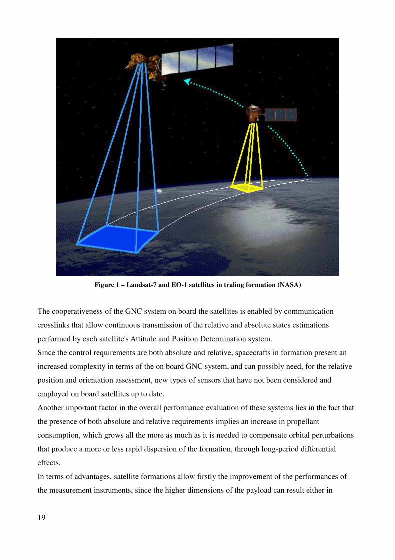
Figure 1 – Landsat-7 and EO-1 satellites in traling formation (NASA)
The cooperativeness of the GNC system on board the satellites is enabled by communication
crosslinks that allow continuous transmission of the relative and absolute states estimations
performed by each satellite's Attitude and Position Determination system.
Since the control requirements are both absolute and relative, spacecrafts in formation present an
increased complexity in terms of the on board GNC system, and can possibly need, for the relative
position and orientation assessment, new types of sensors that have not been considered and
employed on board satellites up to date.
Another important factor in the overall performance evaluation of these systems lies in the fact that
the presence of both absolute and relative requirements implies an increase in propellant
consumption, which grows all the more as much as it is needed to compensate orbital perturbations
that produce a more or less rapid dispersion of the formation, through long-period differential
effects.
In terms of advantages, satellite formations allow firstly the improvement of the performances of
the measurement instruments, since the higher dimensions of the payload can result either in
19
increased measurement area or in increased measurement resolution, or both, wrt single satellite
systems performances on the same type of tasks. Moreover, the formation has a certain degree of
flexibility since the individual GNC system on board each satellite allows to reach and maintain
different configurations, which implies that with this type of satellite system, different kinds of
tasks can be carried out.
The presence of two or more satellites instead of one implies a certain degree of redundance and
robustness to failure. In case of single satellites partial or total failure, the mission tasks can be still
carried out with decreased performances, whereas if replacement satellites are available, the tasks
execution can be resumed with the nominal performances specifications. In both cases, there is no
need to perform a new launch with a replacement satellite so that the execution of the mission tasks
can restart.
One further advantage of cooperative satellites systems is that they result in spacecrafts being more
cost effective, since they are smaller and generally require less development and testing effort in
terms of safety and reliability, being failure probability requirements somewhat relaxed by the
redundance of the system. This implies also reduction of costs associated to the launch system,
since smaller satellites can find more easily accomodation in the fairings of launchers.
One of the main scientific applications for which satellite formation flying systems are intended to
be developed and employed, are interferometric applications. This type of scientific missions can
have the goal of detecting the presence of extrasolar planets that are similar to the Earth, and with
satellites in formation, the detectors can be distributed over large baselines, allowing high
accuracies in the measurements of interferometric fringes. Also, spacecraft formations for
interferometry can be employed for gravitational waves detection in deep space.
Other applications of interest which can be enabled by SFF are Earth missions such as gravitational
field mapping, magnetic field mapping, missions for fundamental physics, Earth imaging through
Synthetic Aperture Radar (SAR), and also military applications, which benefit from the generally
improved and expanded capabilities for communication and imaging tasks.
Nowadays there is already a number of SFF missions that have been successfully operative in orbit.
Others are currently under development for launch in the next years.
The TanDEM-X mission of the DLR, the German Aerospace Agency, consists in two satellites in
formation, each equipped with radar remote sensing instrumentation, with the goal of acquiring a
global Digital Elevation Model (DEM) with unprecedented accuracy, i.e. 12 m in horizontal
resolution and 2 m in relative heighy accuracy, as a new reference for commercial and scientific
applications. The two satellites were launched and started acquisitions in 2010, and successfully
performed the intended mission tasks over the subsequent years.
20
Another successful formation flight mission with two satellites was the GRACE (Gravity Recovery
and Climate Experiment) mission, which derived from a joint partnership between DLR and NASA.
The mission launch was in 2002, with two twin spacecrafts being inserted in the same quasi-polar
orbit at approximately 500 km altitude, with a varying relative distance along the orbital track, up to
200 km. The GRACE satellites have on board laser ranging equipment, accelerometers and GPS
receivers in order to assess precisely their relative position. In this way, precise measurements of
Earth's gravity field anomalies can be performed, which allows to determine important information
for oceanography, geology and climate evolution.
The PRISMA (Prototype Research Instruments and Space Mission technology Advancement)
mission was designed and developed by the Swedish Space Corporation (SSC) in order to
demonstrate formation flight and rendez-vous technologies for orbital servicing. The two PRISMA
satellites were launched in 2010 in a Sun-synchronous, dawn-dusk orbit, and successfully
completed within the end of 2011 all the nominal mission tasks related to autonomous formation
flying, rendez-vous, precision proximity operations, final approach and recede maneuvers.
The Evolved Laser Interferometer Space Antenna (eLISA) is a ESA mission under development for
the next years for the detection and accurate measurement of gravitational waves. In the eLISA
concept there are three spacecrafts in heliocentric orbit, forming a high precision Michelson
interferometer with a baseline of one million kilometers. The distance between each satellite and
another is monitored in order to detect a gravitational wave. In the eLISA constellation concept the
three spacecrafts are orbiting the Sun, trailing 20 degrees behind the Earth. The spacecrafts can be
kept at approximately costant distance from the Earth, or they can be allowed to drift as far away as
70 million km, the maximum distance at which the eLISA communication link with the ground
station can be maintained.
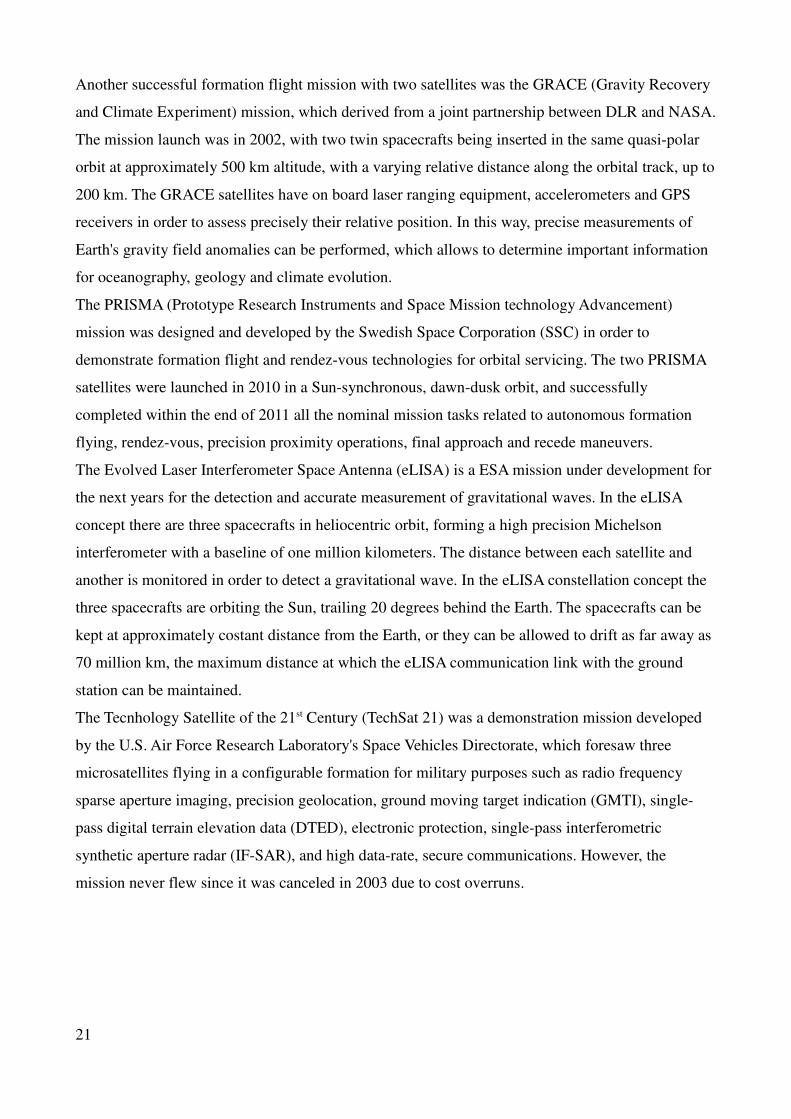
The Tecnhology Satellite of the 21st Century (TechSat 21) was a demonstration mission developed
by the U.S. Air Force Research Laboratory's Space Vehicles Directorate, which foresaw three
microsatellites flying in a configurable formation for military purposes such as radio frequency
sparse aperture imaging, precision geolocation, ground moving target indication (GMTI), single-
pass digital terrain elevation data (DTED), electronic protection, single-pass interferometric
synthetic aperture radar (IF-SAR), and high data-rate, secure communications. However, the
mission never flew since it was canceled in 2003 due to cost overruns.
21
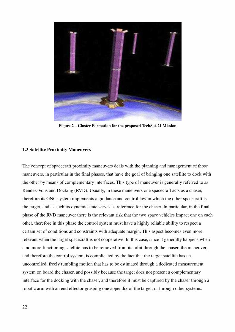
Figure 2 – Cluster Formation for the proposed TechSat-21 Mission
1.3 Satellite Proximity Maneuvers
The concept of spacecraft proximity maneuvers deals with the planning and management of those
maneuvers, in particular in the final phases, that have the goal of bringing one satellite to dock with
the other by means of complementary interfaces. This type of maneuver is generally referred to as
Rendez-Vous and Docking (RVD). Usually, in these maneuvers one spacecraft acts as a chaser,
therefore its GNC system implements a guidance and control law in which the other spacecraft is
the target, and as such its dynamic state serves as reference for the chaser. In particular, in the final
phase of the RVD maneuver there is the relevant risk that the two space vehicles impact one on each
other, therefore in this phase the control system must have a highly reliable ability to respect a
certain set of conditions and constraints with adequate margin. This aspect becomes even more
relevant when the target spacecraft is not cooperative. In this case, since it generally happens when
a no more functioning satellite has to be removed from its orbit through the chaser, the maneuver,
and therefore the control system, is complicated by the fact that the target satellite has an
uncontrolled, freely tumbling motion that has to be estimated through a dedicated measurement
system on board the chaser, and possibly because the target does not present a complementary
interface for the docking with the chaser, and therefore it must be captured by the chaser through a
robotic arm with an end effector grasping one appendix of the target, or through other systems.
22
Up to date, Rendez-Vous and Docking/Capture in currently operative missions is performed as a
non-autonomous maneuver through in the loop intervention of mission operators. In the case of
Autonomous Rendez-vous and Proximity Operations (ARPO) between two spacecrafts, the relative
GNC system must respond to robustness requisites, with the implementation of reliable collision
avoidance and fault management functions. During the last years, a number of missions with
demonstrative purposes have been successful in the on orbit execution of ARPO related
experiments.
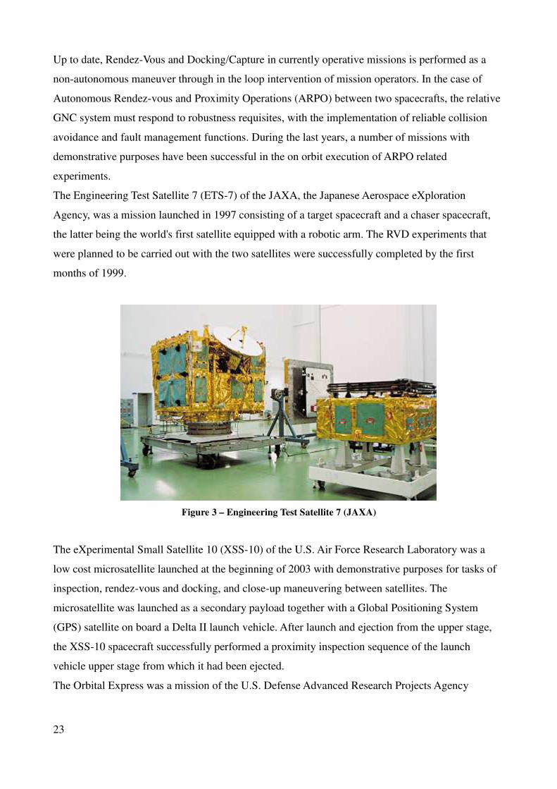
The Engineering Test Satellite 7 (ETS-7) of the JAXA, the Japanese Aerospace eXploration
Agency, was a mission launched in 1997 consisting of a target spacecraft and a chaser spacecraft,
the latter being the world's first satellite equipped with a robotic arm. The RVD experiments that
were planned to be carried out with the two satellites were successfully completed by the first
months of 1999.
Figure 3 – Engineering Test Satellite 7 (JAXA)
The eXperimental Small Satellite 10 (XSS-10) of the U.S. Air Force Research Laboratory was a
low cost microsatellite launched at the beginning of 2003 with demonstrative purposes for tasks of
inspection, rendez-vous and docking, and close-up maneuvering between satellites. The
microsatellite was launched as a secondary payload together with a Global Positioning System
(GPS) satellite on board a Delta II launch vehicle. After launch and ejection from the upper stage,
the XSS-10 spacecraft successfully performed a proximity inspection sequence of the launch
vehicle upper stage from which it had been ejected.
The Orbital Express was a mission of the U.S. Defense Advanced Research Projects Agency
23
(DARPA) and NASA, developed for the demonstration of technologies for rendez-vous, proximity
operations, station keeping, capture, docking, fluid transfer and installation of replaceable units. The
mission consisted in two satellites, a servicing spacecraft with a robotic carrying a vision system-
based navigation system, and a serviceable satellite. The two spacecrafts were launched in 2007,
and in the same year they successfully carried out a RVD experiment, which was followed by an
operation of replacement of the on board computer of the target satellite.
Moreover, in recent years the Front-end Robotics Enabling Near-term Demonstration (FREND)
ground simulator has been developed by DARPA, and successfully tested for the study and
investigation of ARPO tecnhologies and strategies applied to non cooperative targets, e.g. satellites
needing some kind of servicing, but that were built in previous years and were not therefore
equipped with the necessary systems and interfaces for cooperative RVD.
1.4 Original Contributions
Since 2010, the cooperating SPAcecRaft Testbed for Autonomous proximity operatioNs
experimentS (SPARTANS) project is under development and testing at the Center of Studies and
Activities for Space (CISAS) "G. Colombo" of the University of Padova. The goal of the project is
the development and testing of a hardware simulator consisting in two or more units that are
representative of two or more satellites flying in formation or performing a proximity maneuver.
Each Unit of the simulator is made of two main parts. The lower part is the Translation Module
(TM), and it consists in an aluminium structure supporting a suspension system based on air skids,
allowing a low friction motion on a glass surface, and a navigation system which allows position
and Azimuth estimation. The upper part, connected to the TM, is the Attitude Module (AM), which
consists in a 3-axes joint structure, which supports and provides Yaw, Pitch and Roll Degrees of
Freedom (DOF) to an aluminium structure. The aluminium structure of the AM carries an Attitude
Determination System, and a Guidance Navigation and Control System. All Units of the simulator
carry moreover in the AM a Communication System, which allows inter-units crosslinks, and
communications with the external control station, consisting of a laptop through which commands
can be sent and telemetry data can be received. In the final configuration, the simulator can be
employed for extensive studies and investigations of a variety of problems related to SFF, ARPO,
cooperative and non-cooperative Rendez-Vous and Capture. One important aspect of the simulator
is its high level of modularity, allowing fast replacement of equipment for the substitution of no
more functioning components, and also for the installation of systems and sensors, which allows
24
perfomances comparison between different types of hardware on the same tasks.
The SPARTANS project is supervised and directed by Prof. Enrico Lorenzini (CISAS, Department
of Industrial Engineering, University of Padova) and it is carried on by Post doctoral students, Ph.D.
students in Space Sciences Technologies and Measurements, and Master's Degree students in
Aerospace Engineering, with the collaboration of CISAS researchers.
The main contributions of my Ph.D. to the SPARTANS project have been addressed to the design
and development of the TM, to the development and testing of the Optical Flow Sensor (OFS)
navigation system on board the TM for position and Azimuth estimation, to the design and
assembly of the levellable Units test table, to the preliminary planning of position and attitude PID
and optimal control maneuvers through a MATLAB software simulator for the SPARTANS testbed,
and to the software analysis of a satellite inspection scenario for reproduction of relative dynamics
in scale through the SPARTANS simulator.
1.5 Thesis Outline
Chapter 2 presents and describes the SPARTANS simulator and the related development activities.
The subsystems of the AM are described, and subsequently the TM is presented in its main
characteristics and subsystems. Subsequently, a description of the main experimental activities
related to the simulator is provided, concerning the activities addressed to the characterization,
development and testing of the unit's air suspension system, to the design and testing of the
simulator test table, and to development, calibration and testing of the OFS navigation system.
Moreover, the Section presents additional experimental activities that have to be performed, related
to the control thrust force and unit's inertia properties estimation through the torsional wire system
of the Measurements Laboratory.
Chapter 3 presents the preliminary activities related to the integration of the OFS navigation system
with an external Vision-based navigation system, developed in parallel by other Researchers and
PhD students in the context of the SPARTANS project.
Chapter 4 provides firstly a brief description of spacecraft relative motion models, which are
essential in the design and implementation of GNC systems applied to SFF and ARPO problems.
Following the introduction to relative motion models, a description of the Guidance, Navigation and
Control functions is provided, and subsequently different types of control strategies that can be
employed in SFF and/or ARPO problems are presented: Proportional-Integral-Derivative (PID)
control, Linear Quadratic Regulator (LQR), and Model Predictive Control (MPC), of which an
25

explicit solution is presented. After that, a series of position and attitude control maneuvers planned
with the Matlab Software Simulator of the SPARTANS testbed with standard and optimal control
algorithms are presented.
Chapter 5 presents the investigation and related results of a scenario of inspection of a non
cooperative satellite in Low Earth Orbit (LEO), through a spacecraft that has to be inserted in a
Passive Relative Orbit in order to perform the inspection of the non cooperative target. The results
of numerical simulations of the acquisition and maintainance of the inspection orbit are presented,
for the cases of manuevers performed through LQR and MPC optimal controllers.
26

27
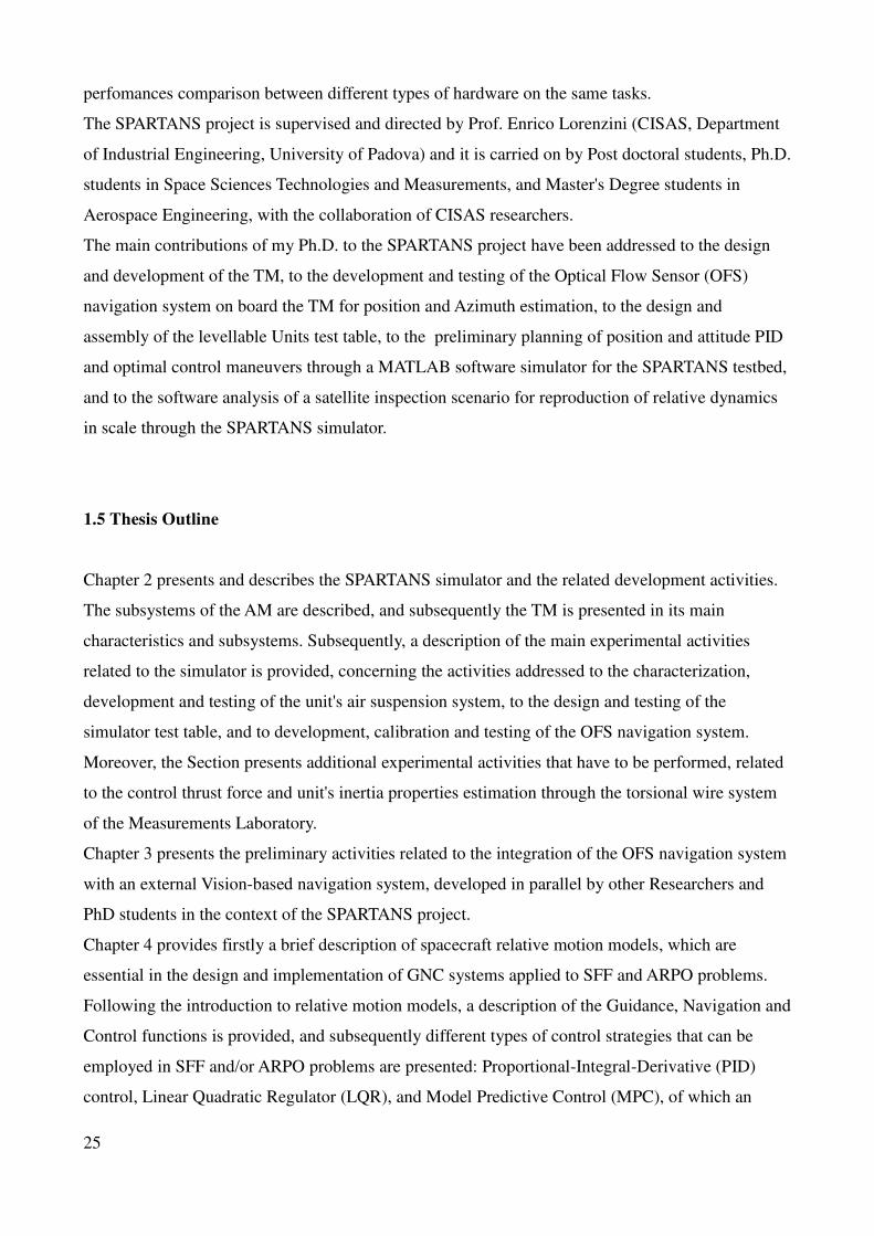
2 SATELLITE PROXIMITY MANEUVERS AND FORMATION FLIGHT HARDWARE
SIMULATOR
In this section the spacecraft hardware simulator called SPARTANS under development at the
CISAS of the University of Padova, is presented in all its main features and functionalities, with a
comprehensive overview of both already developed, and still to be developed components, and
related activities. The simulator is composed by a minimum of two Units, which are robotic
platforms that allow to a certain extent the reproduction of a spacecraft attitude and position motion,
allowing in this way the study and investigation of strategies and problems related to spacecraft
formation flight, Rendez-Vous and Docking (RVD), proximity maneuvers, with hardware-in-the-
loop implementation of Guidance Navigation and Control (GNC) schemes and algorithms.
Figure 4 – The SPARTANS cooperating spacecraft testbed
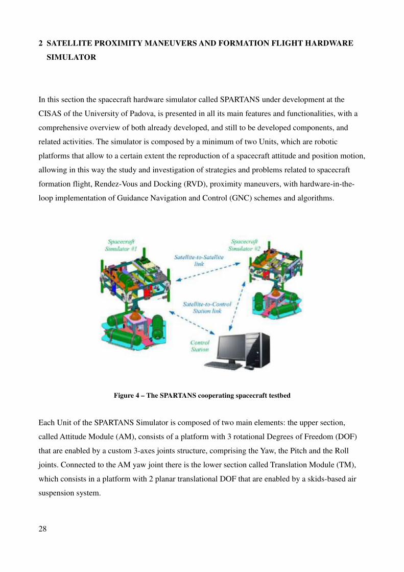
Each Unit of the SPARTANS Simulator is composed of two main elements: the upper section,
called Attitude Module (AM), consists of a platform with 3 rotational Degrees of Freedom (DOF)
that are enabled by a custom 3-axes joints structure, comprising the Yaw, the Pitch and the Roll
joints. Connected to the AM yaw joint there is the lower section called Translation Module (TM),
which consists in a platform with 2 planar translational DOF that are enabled by a skids-based air
suspension system.
28
Figure 5 – The Attitude Module (AM) and the Translation Module (TM)
At the moment of the writing of this thesis the SPARTANS project is at the following stage of
development: a single AM, with only attitude control enabled, has been completed and tested in a
series of attitude control maneuvers up to 3 DOF, with navigation system based on encoders
installed in the joints, and IMU installed onboard the structural components of the module. A single
TM has been developed, completed at the structural level, and its air suspension system tested in
free motion on a glass layer supported by a test table. An incremental and an absolute localization
system for the TM motion estimation (position and Azimuth) have been developed and tested. A
single preliminary Unit has been assembled with the two developed modules, and its free motion
tested on a glass layer supported by a test table.
2.1 Review of Spacecraft Simulators
Testbeds of different types have been used since the beginning of space exploration in order to
validate representative hardware and software together. Table (1) reports the characteristics in terms
of advantages and disadvantages for different types of testbeds.
29
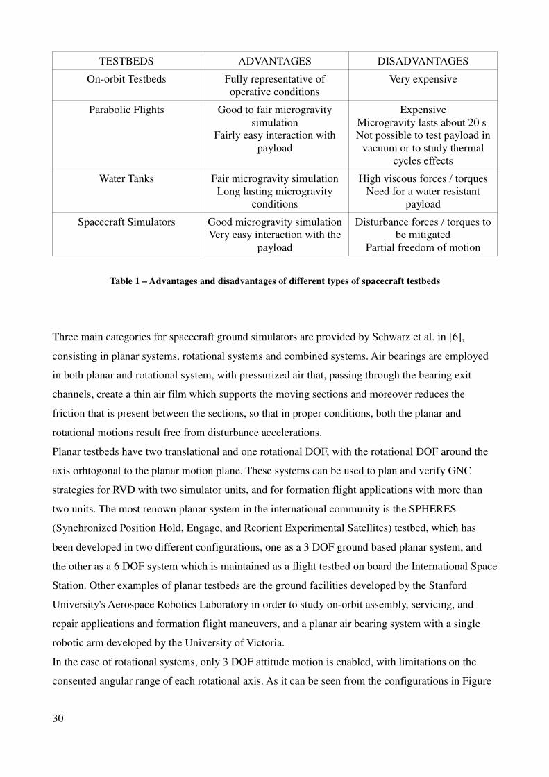
TESTBEDS ADVANTAGES DISADVANTAGES
On-orbit Testbeds Fully representative of
operative conditions
Very expensive
Parabolic Flights Good to fair microgravity
simulation
Fairly easy interaction with
payload
Expensive
Microgravity lasts about 20 s
Not possible to test payload in
vacuum or to study thermal
cycles effects
Water Tanks Fair microgravity simulation
Long lasting microgravity
conditions
High viscous forces / torques
Need for a water resistant
payload
Spacecraft Simulators Good microgravity simulation
Very easy interaction with the
payload
Disturbance forces / torques to
be mitigated
Partial freedom of motion
Table 1 – Advantages and disadvantages of different types of spacecraft testbeds
Three main categories for spacecraft ground simulators are provided by Schwarz et al. in [6],
consisting in planar systems, rotational systems and combined systems. Air bearings are employed
in both planar and rotational system, with pressurized air that, passing through the bearing exit
channels, create a thin air film which supports the moving sections and moreover reduces the
friction that is present between the sections, so that in proper conditions, both the planar and
rotational motions result free from disturbance accelerations.
Planar testbeds have two translational and one rotational DOF, with the rotational DOF around the
axis orhtogonal to the planar motion plane. These systems can be used to plan and verify GNC
strategies for RVD with two simulator units, and for formation flight applications with more than
two units. The most renown planar system in the international community is the SPHERES
(Synchronized Position Hold, Engage, and Reorient Experimental Satellites) testbed, which has
been developed in two different configurations, one as a 3 DOF ground based planar system, and
the other as a 6 DOF system which is maintained as a flight testbed on board the International Space
Station. Other examples of planar testbeds are the ground facilities developed by the Stanford
University's Aerospace Robotics Laboratory in order to study on-orbit assembly, servicing, and
repair applications and formation flight maneuvers, and a planar air bearing system with a single
robotic arm developed by the University of Victoria.
In the case of rotational systems, only 3 DOF attitude motion is enabled, with limitations on the
consented angular range of each rotational axis. As it can be seen from the configurations in Figure
30
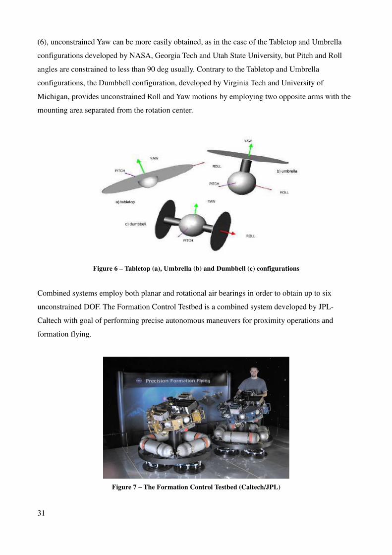
(6), unconstrained Yaw can be more easily obtained, as in the case of the Tabletop and Umbrella
configurations developed by NASA, Georgia Tech and Utah State University, but Pitch and Roll
angles are constrained to less than 90 deg usually. Contrary to the Tabletop and Umbrella
configurations, the Dumbbell configuration, developed by Virginia Tech and University of
Michigan, provides unconstrained Roll and Yaw motions by employing two opposite arms with the
mounting area separated from the rotation center.
Figure 6 – Tabletop (a), Umbrella (b) and Dumbbell (c) configurations
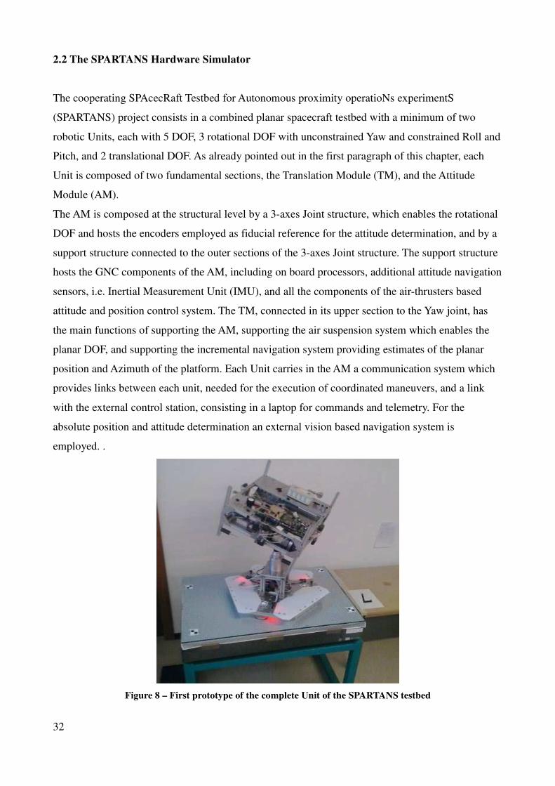
Combined systems employ both planar and rotational air bearings in order to obtain up to six
unconstrained DOF. The Formation Control Testbed is a combined system developed by JPL-
Caltech with goal of performing precise autonomous maneuvers for proximity operations and
formation flying.
Figure 7 – The Formation Control Testbed (Caltech/JPL)
31
2.2 The SPARTANS Hardware Simulator
The cooperating SPAcecRaft Testbed for Autonomous proximity operatioNs experimentS
(SPARTANS) project consists in a combined planar spacecraft testbed with a minimum of two
robotic Units, each with 5 DOF, 3 rotational DOF with unconstrained Yaw and constrained Roll and
Pitch, and 2 translational DOF. As already pointed out in the first paragraph of this chapter, each
Unit is composed of two fundamental sections, the Translation Module (TM), and the Attitude
Module (AM).
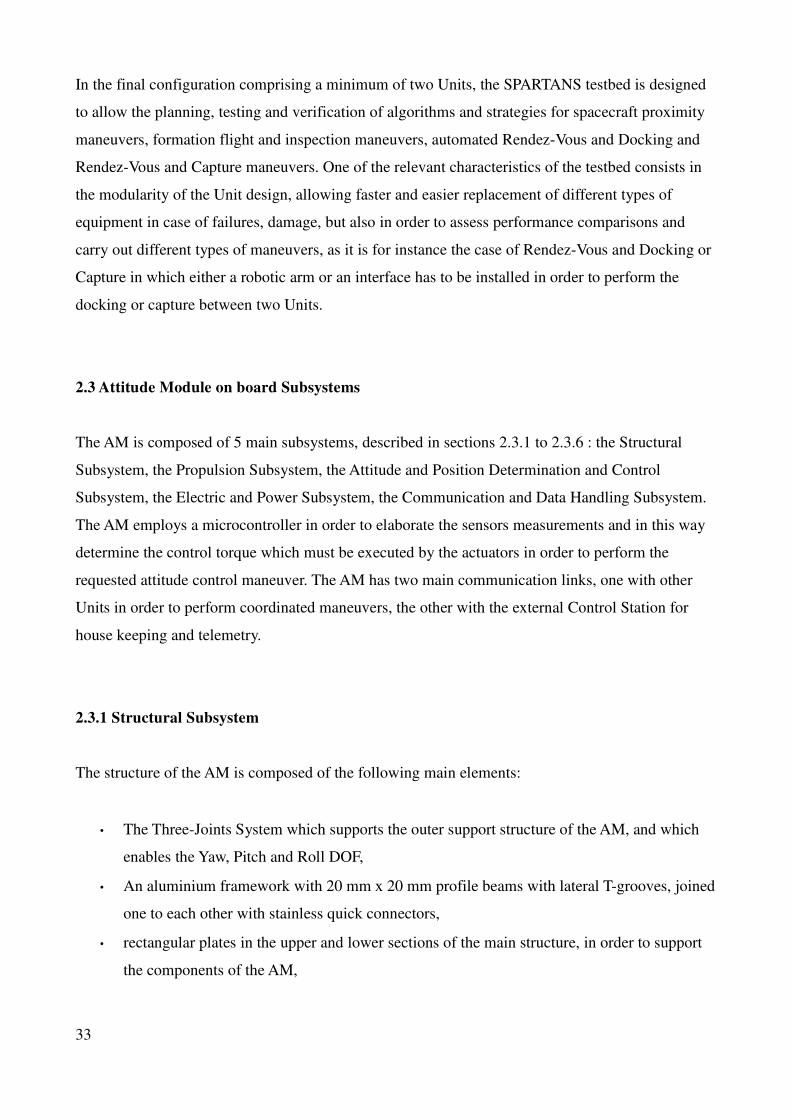
The AM is composed at the structural level by a 3-axes Joint structure, which enables the rotational
DOF and hosts the encoders employed as fiducial reference for the attitude determination, and by a
support structure connected to the outer sections of the 3-axes Joint structure. The support structure
hosts the GNC components of the AM, including on board processors, additional attitude navigation
sensors, i.e. Inertial Measurement Unit (IMU), and all the components of the air-thrusters based
attitude and position control system. The TM, connected in its upper section to the Yaw joint, has
the main functions of supporting the AM, supporting the air suspension system which enables the
planar DOF, and supporting the incremental navigation system providing estimates of the planar
position and Azimuth of the platform. Each Unit carries in the AM a communication system which
provides links between each unit, needed for the execution of coordinated maneuvers, and a link
with the external control station, consisting in a laptop for commands and telemetry. For the
absolute position and attitude determination an external vision based navigation system is
employed. .
Figure 8 – First prototype of the complete Unit of the SPARTANS testbed
32
In the final configuration comprising a minimum of two Units, the SPARTANS testbed is designed
to allow the planning, testing and verification of algorithms and strategies for spacecraft proximity
maneuvers, formation flight and inspection maneuvers, automated Rendez-Vous and Docking and
Rendez-Vous and Capture maneuvers. One of the relevant characteristics of the testbed consists in
the modularity of the Unit design, allowing faster and easier replacement of different types of
equipment in case of failures, damage, but also in order to assess performance comparisons and
carry out different types of maneuvers, as it is for instance the case of Rendez-Vous and Docking or
Capture in which either a robotic arm or an interface has to be installed in order to perform the
docking or capture between two Units.
2.3 Attitude Module on board Subsystems
The AM is composed of 5 main subsystems, described in sections 2.3.1 to 2.3.6 : the Structural
Subsystem, the Propulsion Subsystem, the Attitude and Position Determination and Control
Subsystem, the Electric and Power Subsystem, the Communication and Data Handling Subsystem.
The AM employs a microcontroller in order to elaborate the sensors measurements and in this way
determine the control torque which must be executed by the actuators in order to perform the
requested attitude control maneuver. The AM has two main communication links, one with other
Units in order to perform coordinated maneuvers, the other with the external Control Station for
house keeping and telemetry.
2.3.1 Structural Subsystem
The structure of the AM is composed of the following main elements:
• The Three-Joints System which supports the outer support structure of the AM, and which
enables the Yaw, Pitch and Roll DOF,
• An aluminium framework with 20 mm x 20 mm profile beams with lateral T-grooves, joined
one to each other with stainless quick connectors,
• rectangular plates in the upper and lower sections of the main structure, in order to support
the components of the AM,
33
• reinforcing plates
• support brackets for air-thrust actuators
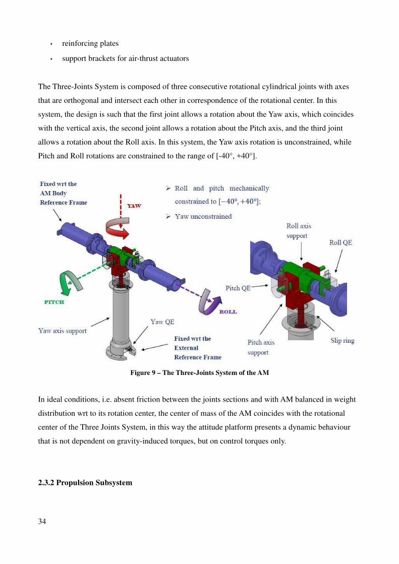
The Three-Joints System is composed of three consecutive rotational cylindrical joints with axes
that are orthogonal and intersect each other in correspondence of the rotational center. In this
system, the design is such that the first joint allows a rotation about the Yaw axis, which coincides
with the vertical axis, the second joint allows a rotation about the Pitch axis, and the third joint
allows a rotation about the Roll axis. In this system, the Yaw axis rotation is unconstrained, while
Pitch and Roll rotations are constrained to the range of [-40°, +40°].
Figure 9 – The Three-Joints System of the AM
In ideal conditions, i.e. absent friction between the joints sections and with AM balanced in weight
distribution wrt to its rotation center, the center of mass of the AM coincides with the rotational
center of the Three Joints System, in this way the attitude platform presents a dynamic behaviour
that is not dependent on gravity-induced torques, but on control torques only.
2.3.2 Propulsion Subsystem
34
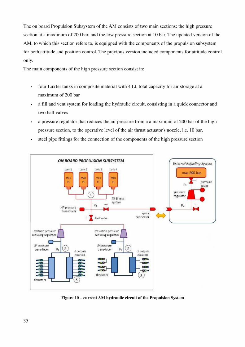
The on board Propulsion Subsystem of the AM consists of two main sections: the high pressure
section at a maximum of 200 bar, and the low pressure section at 10 bar. The updated version of the
AM, to which this section refers to, is equipped with the components of the propulsion subsystem
for both attitude and position control. The previous version included components for attitude control
only.
The main components of the high pressure section consist in:
• four Luxfer tanks in composite material with 4 Lt. total capacity for air storage at a
maximum of 200 bar
• a fill and vent system for loading the hydraulic circuit, consisting in a quick connector and
two ball valves
• a pressure regulator that reduces the air pressure from a a maximum of 200 bar of the high
pressure section, to the operative level of the air thrust actuator's nozzle, i.e. 10 bar,
• steel pipe fittings for the connection of the components of the high pressure section
Figure 10 – current AM hydraulic circuit of the Propulsion System
35
The low pressure section of the AM presents:
• four 6-ways and two 2 double ways manifolds that supply air to the thrusters by distributing
the air flow from the pressure regulator
• 20 air thrusters, 12 for the execution of the command attitude control torques, and 8 for the
execution of the command position control forces
• plastic pipes for the connection of the elements of the low pressure section of the hydraulic
circuit
Each air-thrust actuator is composed by two fundamental elements: an electro-valve and a
converging nozzle. The electro-valve is a solenoid valve which opens upon turning on of its power
supply, and lets the air flow pass to the converging nozzle, while the nozzle consists in a M5 screw
with a central hole of 0.75 mm of diameter.
The actuation axes of the thrusters for both the attitude/position control are disposed so that by
using the four appropriate thrusters for each axis, it is possibile to activate only a positive or
negative torque/force, to be actuated around/along the designed AM Body axis.
2.3.3 Attitude and Position Determination and Control Subsystem
The Attitude and Position Determination and Control Subsystem is composed by the sensors whose
measurements are employed in order to provide an estimation of the AM orientation and planar
position wrt to a Local Vertical Local Horizontal (LVLH) External Frame of Reference, and by the
electronic boards that are in charge of elaborating the sensors measurements in order to compute the
required control action and make it execute by the Propulsion Subsystem.
Each AM carries on board two different types of attitude sensors:
• 3 rotational, incremental optical Quadrature Encoders (QE) which are used to measure the
joints rotation with a 0.09° resolution, providing in this way direct measurements of Yaw,
Pitch and Roll angles
• an Inertial Measurement Unit (IMU) providing AM attitude and attitude rate estimations wrt
to the External Frame of Reference
36
Because of their higher accuracy wrt to the IMU measurements, QE angular measurements are used
as fiducial reference in order to evaluate the IMU measurements drift and bias.
Attitude and position measurements wrt to the External Frame of Reference are moreover
performed by a vision system that is installed outside of the test table, and integrated with the AM
attitude measurements and the TM incremental position measurements.
In the updated version of the AM, the GNC functions are performed by the microcontroller
implemented in a ODROID XU3 single board computer that is installed on board.
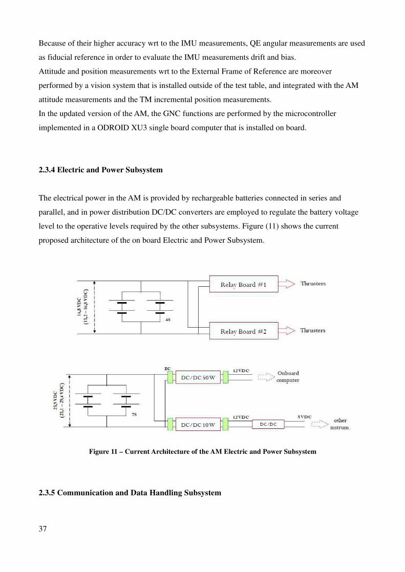
2.3.4 Electric and Power Subsystem
The electrical power in the AM is provided by rechargeable batteries connected in series and
parallel, and in power distribution DC/DC converters are employed to regulate the battery voltage
level to the operative levels required by the other subsystems. Figure (11) shows the current
proposed architecture of the on board Electric and Power Subsystem.
Figure 11 – Current Architecture of the AM Electric and Power Subsystem
2.3.5 Communication and Data Handling Subsystem
37

In the final configuration of the SPARTANS testbed, the Units and the external Control Station
(laptop) use a specific module which allows inter-communication links bewteen Units. For the final
configuration of the testbed, two separate channels are foreseen: a first channel links each Unit to
each other allowing different types of coordinated maneuvers to be carried out, while the second
channel links each Unit to the Control Station, and is allocated to commands and telemetry data
transmission, from the Control Station to Unit and vice-versa, respectively.
The communication protocol consists in variable size packets composed of a header with a
predetermined number of byte, a n-byte data message, and a checksum with a predetermined
number of byte.
The header reports the ID of the transmitting Unit, the ID of the receiving Unit, and the ID
associated to that message. The final checksum in employed for error detection in the transmitted
data.
Units of the simulator can exchange messages that can be grouped in 5 fundamental types:
• Initiate Link Message, used to initialize communications between Units
• Acknowledge Messages, used to verify that commands from the Control Station are
received and executed in synchrony between multiple Units
• Data Request Messages, used by the Control Station to request single or multiple
transmission of telemetry or housekeeping data from the Units
• Data Messages, used by the Units to trasmit telemetry, housekeeping and GNC data
• Command Messages, used to command the execution of a specific operation
2.3.6 On Board and Control Station Software
The on board software in the AM on board computer is organized in 6 main libraries, each with a
main on board process: the Sensors library, the Position and Attitude Determination System (PADS)
library, the Controller (CTRL) library, the Propulsion (PROP) library, the Communication (COMM)
library, the Housekeeping (HKP) library. Each library includes moreover two types of functions: the
Initialization Functions, used for data structures and variables initialization, or re-initialization, and
the Update Functions, used to update the library variables, such as current dynamic state updating
and control action computation
The microcontroller implemented in the onboard computer implements two types of processes.
38
Periodic Interrupt Processes execute actions that are repetitive and time-dependent, e.g. GNC
related operations. Event-driven background and GNC tasks on the other hand are employed in the
implementation of non time-dependent operations, e.g. software initialization, formation flight
scheme change, activation of collosion avoidance schemes, etc. GNC operations that are periodic
need to be synchronized since control actions must be computed and above all executed when
sensors data are updated.
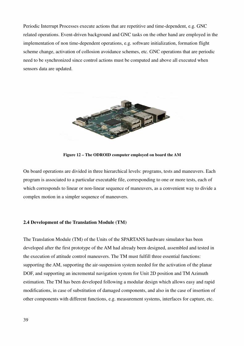
Figure 12 – The ODROID computer employed on board the AM
On board operations are divided in three hierarchical levels: programs, tests and maneuvers. Each
program is associated to a particular executable file, corresponding to one or more tests, each of
which corresponds to linear or non-linear sequence of maneuvers, as a convenient way to divide a
complex motion in a simpler sequence of maneuvers.
2.4 Development of the Translation Module (TM)
The Translation Module (TM) of the Units of the SPARTANS hardware simulator has been
developed after the first prototype of the AM had already been designed, assembled and tested in
the execution of attitude control maneuvers. The TM must fulfill three essential functions:
supporting the AM, supporting the air-suspension system needed for the activation of the planar
DOF, and supporting an incremental navigation system for Unit 2D position and TM Azimuth
estimation. The TM has been developed following a modular design which allows easy and rapid
modifications, in case of substitution of damaged components, and also in the case of insertion of
other components with different functions, e.g. measurement systems, interfaces for capture, etc.
39
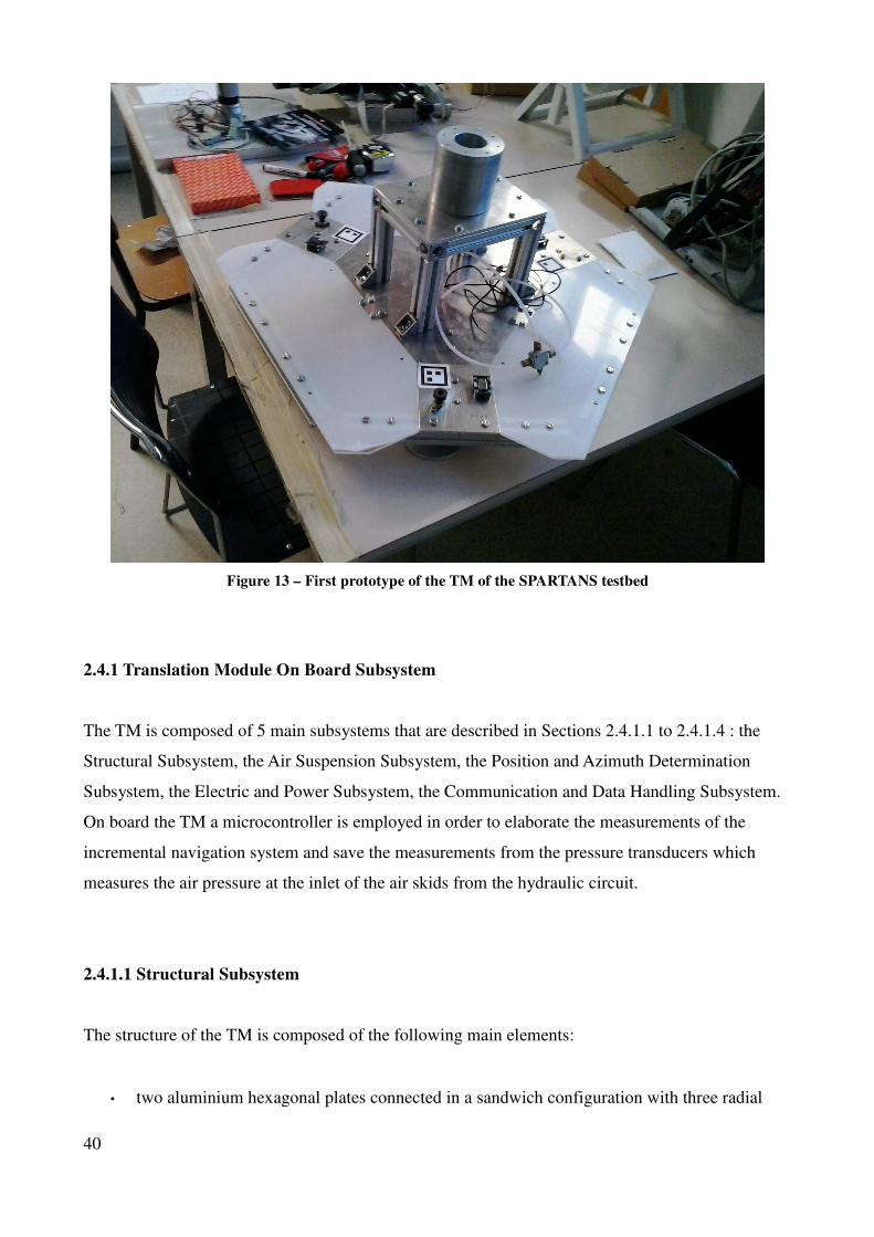
Figure 13 – First prototype of the TM of the SPARTANS testbed
2.4.1 Translation Module On Board Subsystem
The TM is composed of 5 main subsystems that are described in Sections 2.4.1.1 to 2.4.1.4 : the
Structural Subsystem, the Air Suspension Subsystem, the Position and Azimuth Determination
Subsystem, the Electric and Power Subsystem, the Communication and Data Handling Subsystem.
On board the TM a microcontroller is employed in order to elaborate the measurements of the
incremental navigation system and save the measurements from the pressure transducers which
measures the air pressure at the inlet of the air skids from the hydraulic circuit.
2.4.1.1 Structural Subsystem
The structure of the TM is composed of the following main elements:
• two aluminium hexagonal plates connected in a sandwich configuration with three radial
40
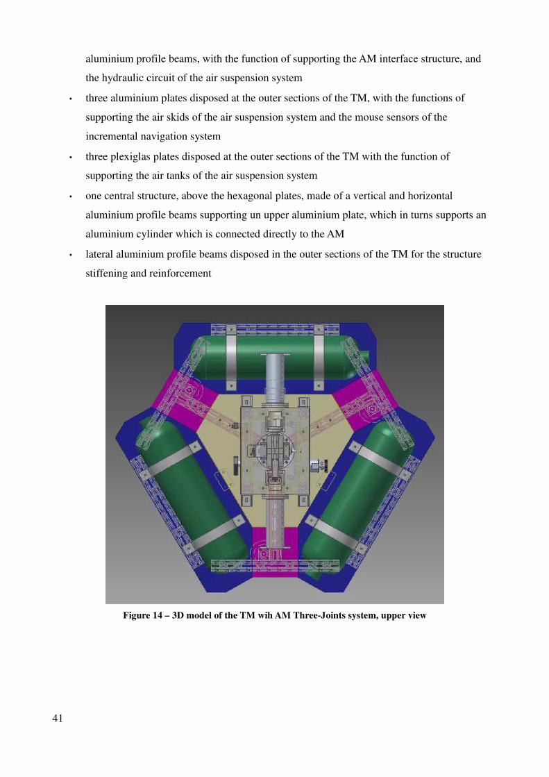
aluminium profile beams, with the function of supporting the AM interface structure, and
the hydraulic circuit of the air suspension system
• three aluminium plates disposed at the outer sections of the TM, with the functions of
supporting the air skids of the air suspension system and the mouse sensors of the
incremental navigation system
• three plexiglas plates disposed at the outer sections of the TM with the function of
supporting the air tanks of the air suspension system
• one central structure, above the hexagonal plates, made of a vertical and horizontal
aluminium profile beams supporting un upper aluminium plate, which in turns supports an
aluminium cylinder which is connected directly to the AM
• lateral aluminium profile beams disposed in the outer sections of the TM for the structure
stiffening and reinforcement
Figure 14 – 3D model of the TM wih AM Three-Joints system, upper view
41
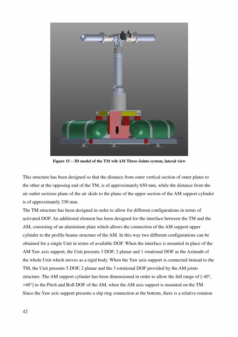
Figure 15 – 3D model of the TM wih AM Three-Joints system, lateral view
This structure has been designed so that the distance from outer vertical section of outer plates to
the other at the opposing end of the TM, is of approximately 650 mm, while the distance from the
air outlet sections plane of the air skids to the plane of the upper section of the AM support cylinder
is of approximately 330 mm.
The TM structure has been designed in order to allow for different configurations in terms of
activated DOF. An additional element has been designed for the interface between the TM and the
AM, consisting of an aluminium plate which allows the connection of the AM support upper
cylinder to the profile beams structure of the AM. In this way two different configurations can be
obtained for a single Unit in terms of available DOF. When the interface is mounted in place of the
AM Yaw axis support, the Unit presents 3 DOF, 2 planar and 1 rotational DOF as the Azimuth of
the whole Unit which moves as a rigid body. When the Yaw axis support is connected instead to the
TM, the Unit presents 5 DOF, 2 planar and the 3 rotational DOF provided by the AM joints
structure. The AM support cylinder has been dimensioned in order to allow the full range of [-40°,
+40°] to the Pitch and Roll DOF of the AM, when the AM axis support is mounted on the TM.
Since the Yaw axis support presents a slip ring connection at the bottom, there is a relative rotation
42
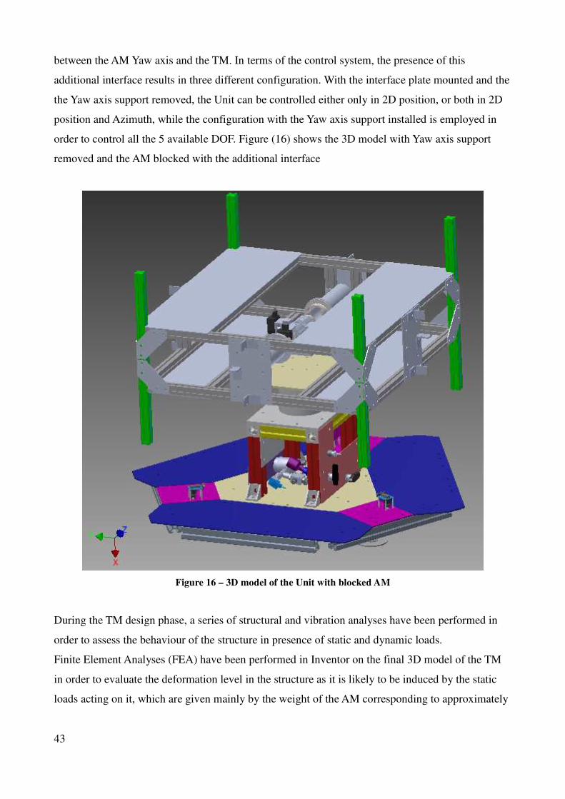
between the AM Yaw axis and the TM. In terms of the control system, the presence of this
additional interface results in three different configuration. With the interface plate mounted and the
the Yaw axis support removed, the Unit can be controlled either only in 2D position, or both in 2D
position and Azimuth, while the configuration with the Yaw axis support installed is employed in
order to control all the 5 available DOF. Figure (16) shows the 3D model with Yaw axis support
removed and the AM blocked with the additional interface
Figure 16 – 3D model of the Unit with blocked AM
During the TM design phase, a series of structural and vibration analyses have been performed in
order to assess the behaviour of the structure in presence of static and dynamic loads.
Finite Element Analyses (FEA) have been performed in Inventor on the final 3D model of the TM
in order to evaluate the deformation level in the structure as it is likely to be induced by the static
loads acting on it, which are given mainly by the weight of the AM corresponding to approximately
43
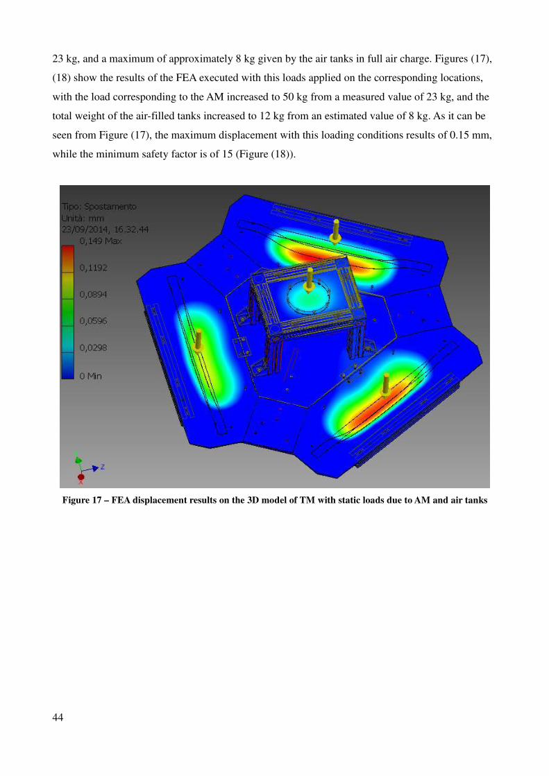
23 kg, and a maximum of approximately 8 kg given by the air tanks in full air charge. Figures (17),
(18) show the results of the FEA executed with this loads applied on the corresponding locations,
with the load corresponding to the AM increased to 50 kg from a measured value of 23 kg, and the
total weight of the air-filled tanks increased to 12 kg from an estimated value of 8 kg. As it can be
seen from Figure (17), the maximum displacement with this loading conditions results of 0.15 mm,
while the minimum safety factor is of 15 (Figure (18)).
Figure 17 – FEA displacement results on the 3D model of TM with static loads due to AM and air tanks
44
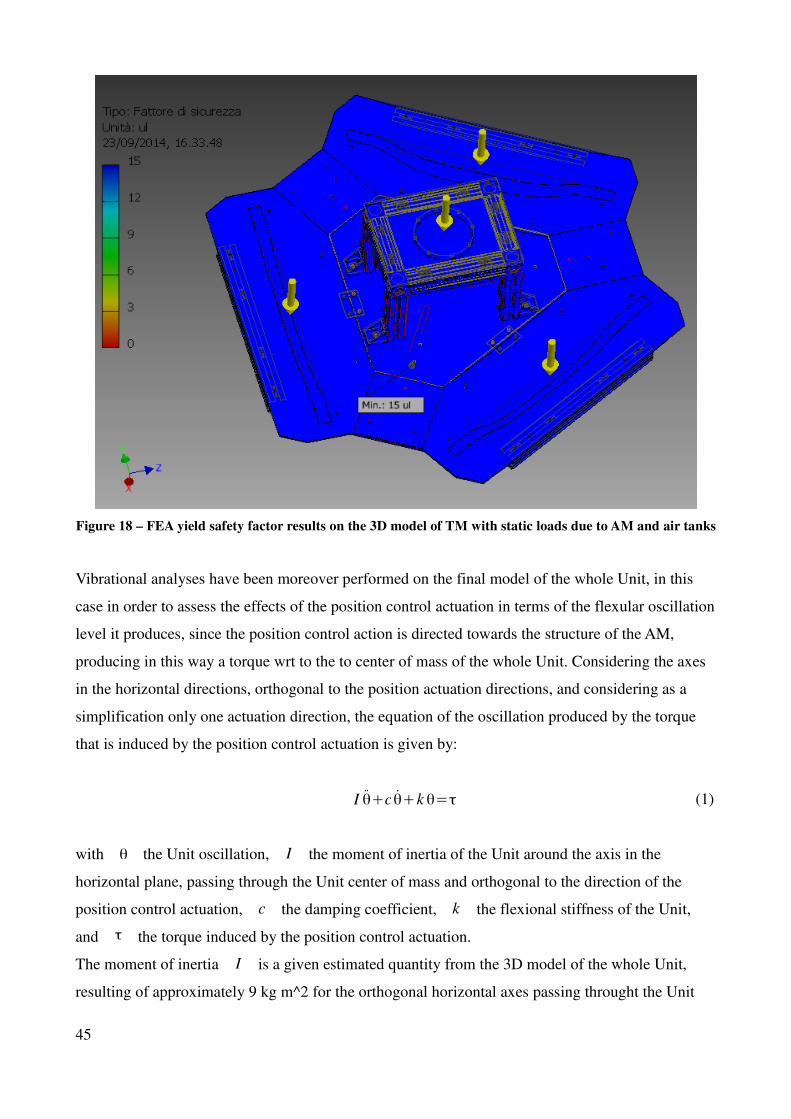
Figure 18 – FEA yield safety factor results on the 3D model of TM with static loads due to AM and air tanks
Vibrational analyses have been moreover performed on the final model of the whole Unit, in this
case in order to assess the effects of the position control actuation in terms of the flexular oscillation
level it produces, since the position control action is directed towards the structure of the AM,
producing in this way a torque wrt to the to center of mass of the whole Unit. Considering the axes
in the horizontal directions, orthogonal to the position actuation directions, and considering as a
simplification only one actuation direction, the equation of the oscillation produced by the torque
that is induced by the position control actuation is given by:
I θ+c θ+k θ=τ (1)
with θ the Unit oscillation, I the moment of inertia of the Unit around the axis in the
horizontal plane, passing through the Unit center of mass and orthogonal to the direction of the
position control actuation, c the damping coefficient, k the flexional stiffness of the Unit,
and τ the torque induced by the position control actuation.
The moment of inertia I is a given estimated quantity from the 3D model of the whole Unit,
resulting of approximately 9 kg m^2 for the orthogonal horizontal axes passing throught the Unit
45
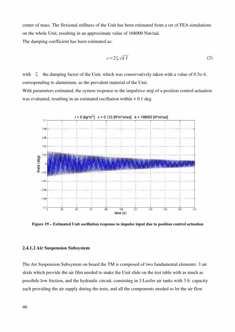
center of mass. The flexional stiffness of the Unit has been estimated from a set of FEA simulations
on the whole Unit, resulting in an approximate value of 168000 Nm/rad.
The damping coefficient has been estimated as:
c=2ζ√k I (2)
with ζ the damping factor of the Unit, which was conservatively taken with a value of 0.5e-4,
corresponding to aluminium, as the prevalent material of the Unit.
With parameters estimated, the system response to the impulsive step of a position control actuation
was evaluated, resulting in an estimated oscillation within ± 0.1 deg.
Figure 19 – Estimated Unit oscillation response to impulse input due to position control actuation
2.4.1.2 Air Suspension Subsystem
The Air Suspension Subsystem on board the TM is composed of two fundamental elements: 3 air
skids which provide the air film needed to make the Unit slide on the test table with as much as
possibile low friction, and the hydraulic circuit, consisting in 3 Luxfer air tanks with 3 lt. capacity
each providing the air supply during the tests, and all the components needed to let the air flow
46
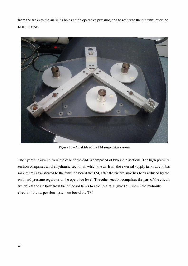
from the tanks to the air skids holes at the operative pressure, and to recharge the air tanks after the
tests are over.
Figure 20 – Air skids of the TM suspension system
The hydraulic circuit, as in the case of the AM is composed of two main sections. The high pressure
section comprises all the hydraulic section in which the air from the external supply tanks at 200 bar
maximum is transferred to the tanks on board the TM, after the air pressure has been reduced by the
on board pressure regulator to the operative level. The other section comprises the part of the circuit
which lets the air flow from the on board tanks to skids outlet. Figure (21) shows the hydraulic
circuit of the suspension system on board the TM
47
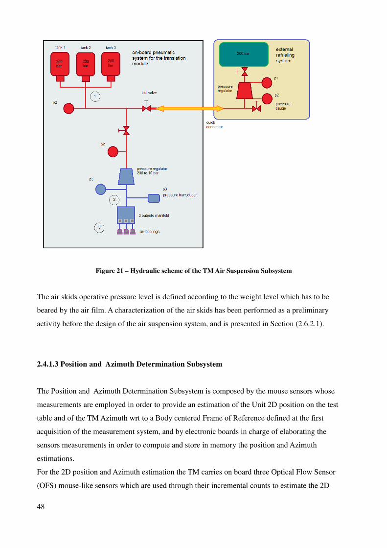
Figure 21 – Hydraulic scheme of the TM Air Suspension Subsystem
The air skids operative pressure level is defined according to the weight level which has to be
beared by the air film. A characterization of the air skids has been performed as a preliminary
activity before the design of the air suspension system, and is presented in Section (2.6.2.1).
2.4.1.3 Position and Azimuth Determination Subsystem
The Position and Azimuth Determination Subsystem is composed by the mouse sensors whose
measurements are employed in order to provide an estimation of the Unit 2D position on the test
table and of the TM Azimuth wrt to a Body centered Frame of Reference defined at the first
acquisition of the measurement system, and by electronic boards in charge of elaborating the
sensors measurements in order to compute and store in memory the position and Azimuth
estimations.
For the 2D position and Azimuth estimation the TM carries on board three Optical Flow Sensor
(OFS) mouse-like sensors which are used through their incremental counts to estimate the 2D
48
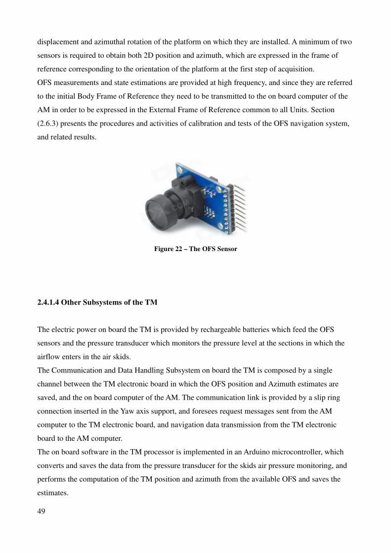
displacement and azimuthal rotation of the platform on which they are installed. A minimum of two
sensors is required to obtain both 2D position and azimuth, which are expressed in the frame of
reference corresponding to the orientation of the platform at the first step of acquisition.
OFS measurements and state estimations are provided at high frequency, and since they are referred
to the initial Body Frame of Reference they need to be transmitted to the on board computer of the
AM in order to be expressed in the External Frame of Reference common to all Units. Section
(2.6.3) presents the procedures and activities of calibration and tests of the OFS navigation system,
and related results.
Figure 22 – The OFS Sensor
2.4.1.4 Other Subsystems of the TM
The electric power on board the TM is provided by rechargeable batteries which feed the OFS
sensors and the pressure transducer which monitors the pressure level at the sections in which the
airflow enters in the air skids.
The Communication and Data Handling Subsystem on board the TM is composed by a single
channel between the TM electronic board in which the OFS position and Azimuth estimates are
saved, and the on board computer of the AM. The communication link is provided by a slip ring
connection inserted in the Yaw axis support, and foresees request messages sent from the AM
computer to the TM electronic board, and navigation data transmission from the TM electronic
board to the AM computer.
The on board software in the TM processor is implemented in an Arduino microcontroller, which
converts and saves the data from the pressure transducer for the skids air pressure monitoring, and
performs the computation of the TM position and azimuth from the available OFS and saves the
estimates.
49
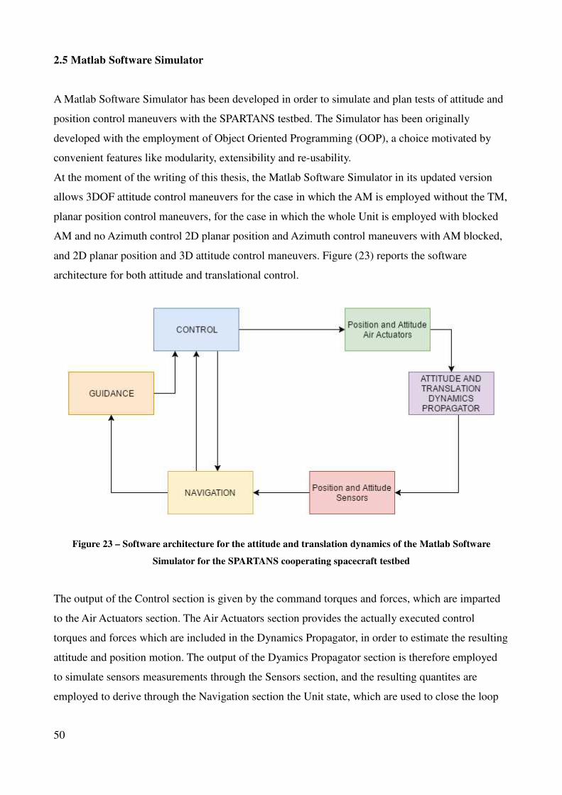
2.5 Matlab Software Simulator
A Matlab Software Simulator has been developed in order to simulate and plan tests of attitude and
position control maneuvers with the SPARTANS testbed. The Simulator has been originally
developed with the employment of Object Oriented Programming (OOP), a choice motivated by
convenient features like modularity, extensibility and re-usability.
At the moment of the writing of this thesis, the Matlab Software Simulator in its updated version
allows 3DOF attitude control maneuvers for the case in which the AM is employed without the TM,
planar position control maneuvers, for the case in which the whole Unit is employed with blocked
AM and no Azimuth control 2D planar position and Azimuth control maneuvers with AM blocked,
and 2D planar position and 3D attitude control maneuvers. Figure (23) reports the software
architecture for both attitude and translational control.
Figure 23 – Software architecture for the attitude and translation dynamics of the Matlab Software
Simulator for the SPARTANS cooperating spacecraft testbed
The output of the Control section is given by the command torques and forces, which are imparted
to the Air Actuators section. The Air Actuators section provides the actually executed control
torques and forces which are included in the Dynamics Propagator, in order to estimate the resulting
attitude and position motion. The output of the Dyamics Propagator section is therefore employed
to simulate sensors measurements through the Sensors section, and the resulting quantites are
employed to derive through the Navigation section the Unit state, which are used to close the loop
50
with the determination of the Control command actions and the state reference from the Guidance
section.
The Simulator features implementation of two fundamental types of controllers, Standard and
Optimal controllers. For standard control, a Proportional Derivative Integral (PID) controller for
both Attitude and Position is implemented with a proportional and derivative kick avoidance
scheme and anti-reset windup scheme, (see Section 4.2.3.1 for details on PID formulation ). The
PID controller is implemented in both continuous and discretized formulations.
With regards to optimal controllers, Model Predictive Control (MPC) and Linear Quadratic
Regulator (LQR) have been implemented for both Attitude and Position control maneuvers. The
MPC controller is implemented in both implicit and explicit formulation (see Sections 4.2.3.2 and
4.2.3.3 for details on LQR and MPC formulations, respectively). A series of simulated control
maneuvers performed with the Software Simulator are presented in Chapter 4.
The Guidance module is able to implent pseudospectral optimal control methods for attitude and
position reference trajectories. Pseudospectral methods solve optimal control problems through
approximation of state and control variables as weighted sum of Legendre or Chebyshev
polynomial basis, resulting in a set of algebraic equations given by the discretization of differential
equations and constraints of the optimal control problem over a grid of orthogonal collocation
nodes, and integration in the cost functional approximated by Gauss quadrature rules. The original
optimal control problem is therefore transformed into a linear programming problem which is
solved numerically through a sparse nonlinear programming solver. Pseudospectral methods are
characterized by a exponential (spectral) rate of convergence, faster than any polynomial rate, and
good accuracy achievable over coarse grids.
2.6 Experimental and other activites related to the development of the SPARTANS testbed
This Sections presents a series of experimental and additional activities that have been performed
for the development of the SPARTANS cooperating spacecraft testbed. As already pointed out in the
Thesis Outline, the main contributions of my PhD in terms of these activities consisted in the Air
suspension system and test table development, and in the development and testing of the Optical
Flow Sensor (OFS) navigation system. Activities related to Thrust force estimation and Inertia
properties determination through the Torque Wire system of the Measurements Laboratory are
briefly presented as a small contribution at the beginning of the PhD with the first prototype of the
AM, and as planned to be performed for the characterization of the first prototype of the complete
51
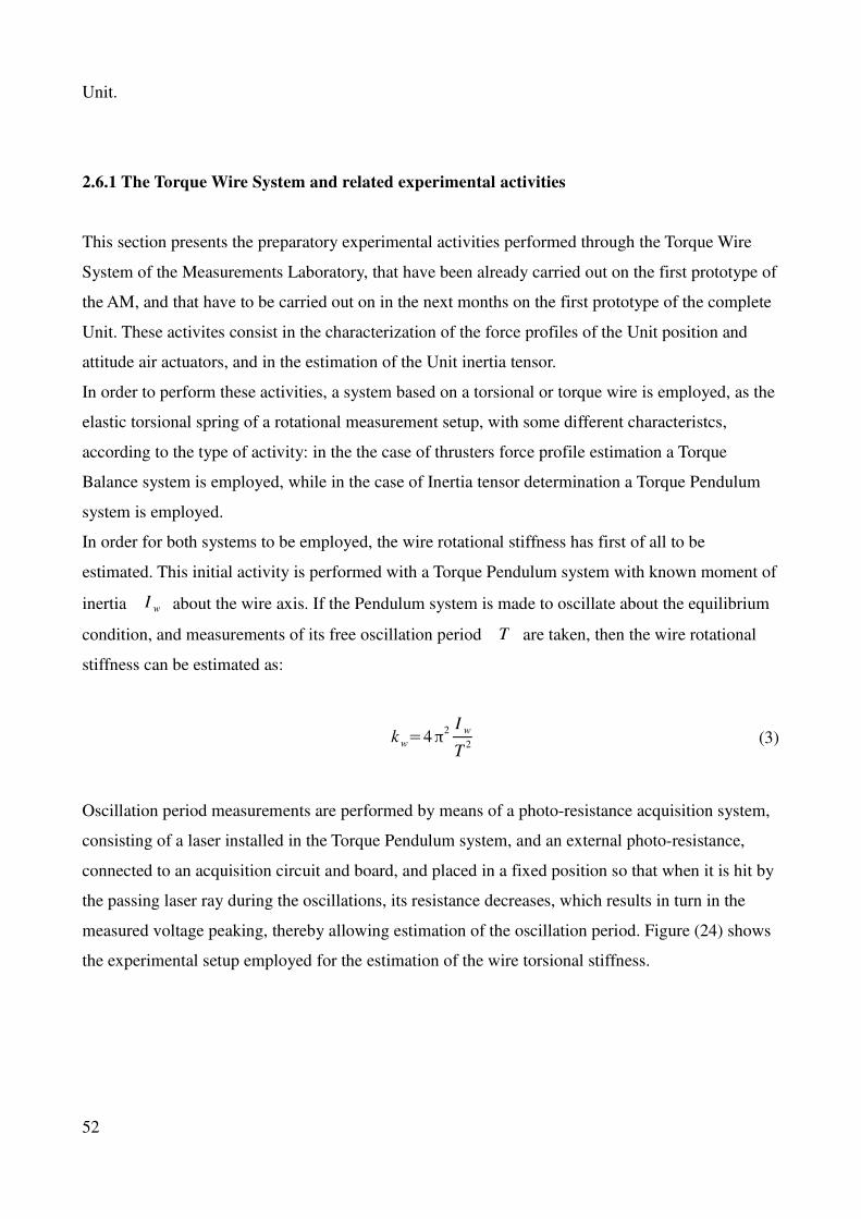
Unit.
2.6.1 The Torque Wire System and related experimental activities
This section presents the preparatory experimental activities performed through the Torque Wire
System of the Measurements Laboratory, that have been already carried out on the first prototype of
the AM, and that have to be carried out on in the next months on the first prototype of the complete
Unit. These activites consist in the characterization of the force profiles of the Unit position and
attitude air actuators, and in the estimation of the Unit inertia tensor.
In order to perform these activities, a system based on a torsional or torque wire is employed, as the
elastic torsional spring of a rotational measurement setup, with some different characteristcs,
according to the type of activity: in the the case of thrusters force profile estimation a Torque
Balance system is employed, while in the case of Inertia tensor determination a Torque Pendulum
system is employed.
In order for both systems to be employed, the wire rotational stiffness has first of all to be
estimated. This initial activity is performed with a Torque Pendulum system with known moment of
inertia I w about the wire axis. If the Pendulum system is made to oscillate about the equilibrium
condition, and measurements of its free oscillation period T are taken, then the wire rotational
stiffness can be estimated as:
k w=4π2 I w
T2 (3)
Oscillation period measurements are performed by means of a photo-resistance acquisition system,
consisting of a laser installed in the Torque Pendulum system, and an external photo-resistance,
connected to an acquisition circuit and board, and placed in a fixed position so that when it is hit by
the passing laser ray during the oscillations, its resistance decreases, which results in turn in the
measured voltage peaking, thereby allowing estimation of the oscillation period. Figure (24) shows
the experimental setup employed for the estimation of the wire torsional stiffness.
52
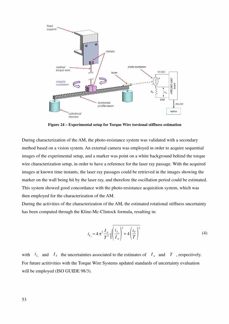
Figure 24 – Experimental setup for Torque Wire torsional stiffness estimation
During characterization of the AM, the photo-resistance system was validated with a secondary
method based on a vision system. An external camera was employed in order to acquire sequential
images of the experimental setup, and a marker was point on a white background behind the torque
wire characterization setup, in order to have a reference for the laser ray passage. With the acquired
images at known time instants, the laser ray passages could be retrieved in the images showing the
marker on the wall being hit by the laser ray, and therefore the oscillation period could be estimated.
This system showed good concordance with the photo-resistance acquisition system, which was
then employed for the characterization of the AM.
During the activities of the characterization of the AM, the estimated rotational stiffness uncertainty
has been computed through the Kline-Mc-Clintock formula, resulting in:
ik w=4π2 I w
T2 √(
i I w
I w)
2
+4(iT
T )2
(4)
with i Iwand I T the uncertainties associated to the estimates of I w and T , respectively.
For future actitivities with the Torque Wire Systems updated standards of uncertainty evaluation
will be employed (ISO GUIDE 98/3).
53
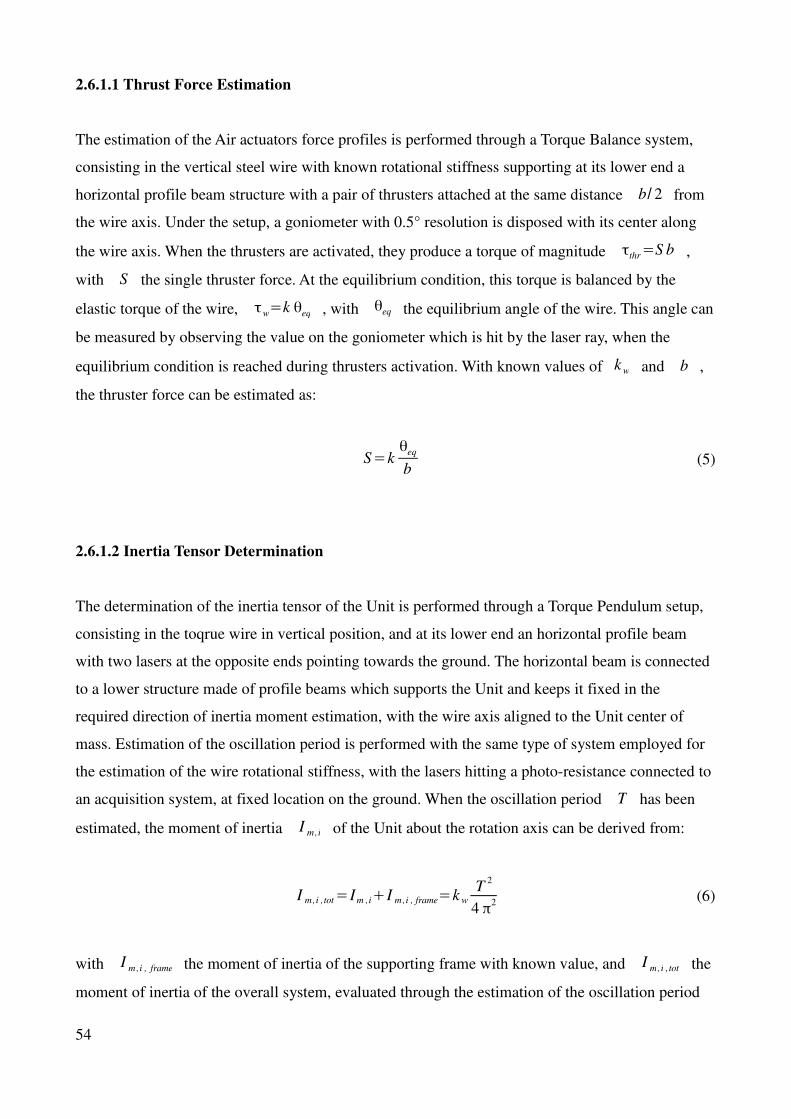
2.6.1.1 Thrust Force Estimation
The estimation of the Air actuators force profiles is performed through a Torque Balance system,
consisting in the vertical steel wire with known rotational stiffness supporting at its lower end a
horizontal profile beam structure with a pair of thrusters attached at the same distance b/ 2 from
the wire axis. Under the setup, a goniometer with 0.5° resolution is disposed with its center along
the wire axis. When the thrusters are activated, they produce a torque of magnitude τthr=S b ,
with S the single thruster force. At the equilibrium condition, this torque is balanced by the
elastic torque of the wire, τw=k θeq , with θeq the equilibrium angle of the wire. This angle can
be measured by observing the value on the goniometer which is hit by the laser ray, when the
equilibrium condition is reached during thrusters activation. With known values of k w and b ,
the thruster force can be estimated as:
S=kθeq
b (5)
2.6.1.2 Inertia Tensor Determination
The determination of the inertia tensor of the Unit is performed through a Torque Pendulum setup,
consisting in the toqrue wire in vertical position, and at its lower end an horizontal profile beam
with two lasers at the opposite ends pointing towards the ground. The horizontal beam is connected
to a lower structure made of profile beams which supports the Unit and keeps it fixed in the
required direction of inertia moment estimation, with the wire axis aligned to the Unit center of
mass. Estimation of the oscillation period is performed with the same type of system employed for
the estimation of the wire rotational stiffness, with the lasers hitting a photo-resistance connected to
an acquisition system, at fixed location on the ground. When the oscillation period T has been
estimated, the moment of inertia I m,i of the Unit about the rotation axis can be derived from:
I m,i ,tot=Im ,i+I m,i , frame=k w
T2
4 π2 (6)
with I m,i , frame the moment of inertia of the supporting frame with known value, and I m,i ,tot the
moment of inertia of the overall system, evaluated through the estimation of the oscillation period
54
of the Torque Pendulum.
The vector of 6 independent components x=[ J xx , J xy , J xz , J yy , J yz , J zz ]T
of the inertia tensor
referenced to the Body frame, is related to the measurements vector of the inertia moment I m
through the linear equation system A x= I m , with matrix A having components dependent on
the measurements directions. The 6 components of the inertia tensor can therefore be estimated as
x=(ATA )
− 1
AT
I m.
2.6.2 Development and testing of the Unit Air Suspension System and of the Simulator Test
Table
This section presents the activities related to the development of the skids-based air suspension
system enabling the planar translation motion of the Units of the Simulator, and the development of
a levelable table supporting the Units of the Simulator and allowing a low friction and balanced
translation motion through the air suspension system.
2.6.2.1 Development and testing of the Unit Air Suspension System
In order to provide 2 translational DOF to the Unit of the simulator, a suspension system based on
air skids has been developed and tested. For the first prototype of the Simulator Unit, the skids
available in the Measurements Laboratory have been tested and employed in the design of the TM.
The modular design of the TM allows an easy replacement of the sections supporting the air
suspension system in case of substitution of the skids for the first prototype of the Unit, or in case of
different skids design for the other Unit/Units that will be developed and assembled.
The main activity related to the development of the air suspension system consisted in the
characterization of the skids installed on a platform that allowed insertion of additional loads on it.
The skids were fed through an external compressor with 50 Lt capacity, providing air at a maximum
of 8 bar, and decreasing in time during the fillout of the compressor tank.
Two main aspects have been studied through the laboratory tests. The first aspect is related to the
motion smoothness according to a certain pressure with which the air is provided to the skids in
order to create the film that allows the suspension of the platform and consequently enables the
planar motion on the test table. This aspect was evaluated empirically, varying the air pressure level
55
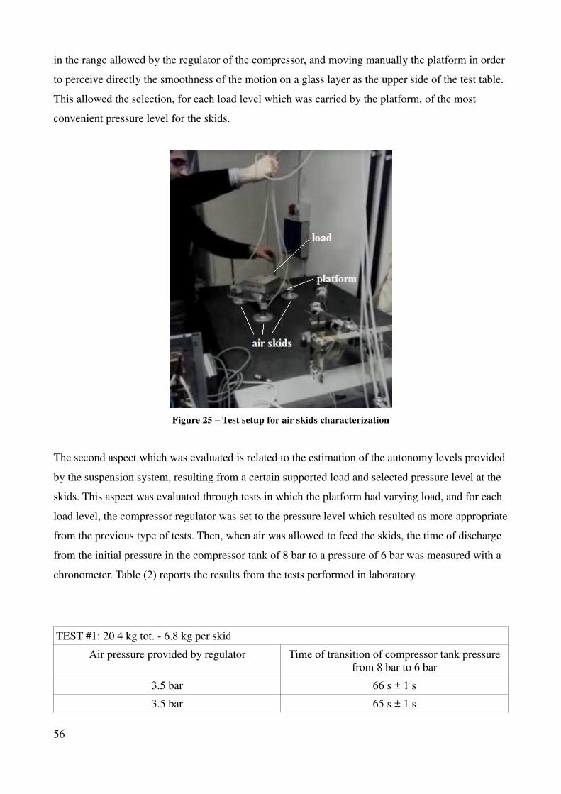
in the range allowed by the regulator of the compressor, and moving manually the platform in order
to perceive directly the smoothness of the motion on a glass layer as the upper side of the test table.
This allowed the selection, for each load level which was carried by the platform, of the most
convenient pressure level for the skids.
Figure 25 – Test setup for air skids characterization
The second aspect which was evaluated is related to the estimation of the autonomy levels provided
by the suspension system, resulting from a certain supported load and selected pressure level at the
skids. This aspect was evaluated through tests in which the platform had varying load, and for each
load level, the compressor regulator was set to the pressure level which resulted as more appropriate
from the previous type of tests. Then, when air was allowed to feed the skids, the time of discharge
from the initial pressure in the compressor tank of 8 bar to a pressure of 6 bar was measured with a
chronometer. Table (2) reports the results from the tests performed in laboratory.
TEST #1: 20.4 kg tot. - 6.8 kg per skid
Air pressure provided by regulator Time of transition of compressor tank pressure
from 8 bar to 6 bar
3.5 bar 66 s ± 1 s
3.5 bar 65 s ± 1 s
56
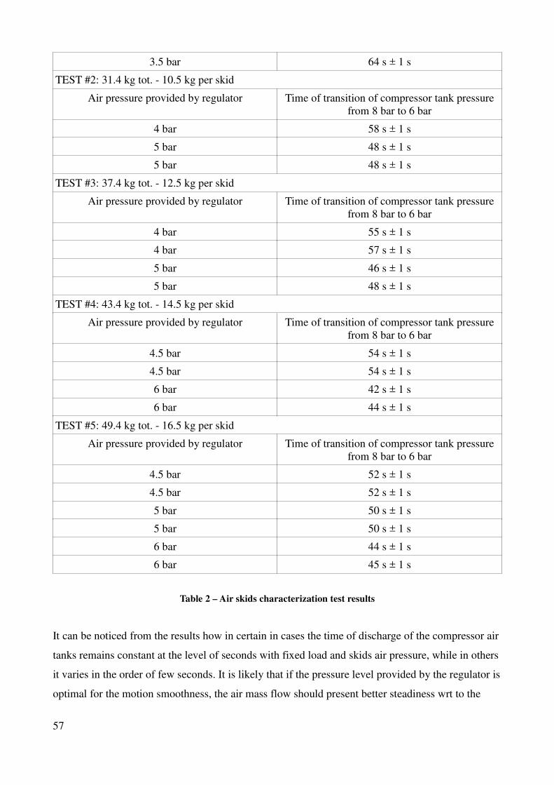
3.5 bar 64 s ± 1 s
TEST #2: 31.4 kg tot. - 10.5 kg per skid
Air pressure provided by regulator Time of transition of compressor tank pressure
from 8 bar to 6 bar
4 bar 58 s ± 1 s
5 bar 48 s ± 1 s
5 bar 48 s ± 1 s
TEST #3: 37.4 kg tot. - 12.5 kg per skid
Air pressure provided by regulator Time of transition of compressor tank pressure
from 8 bar to 6 bar
4 bar 55 s ± 1 s
4 bar 57 s ± 1 s
5 bar 46 s ± 1 s
5 bar 48 s ± 1 s
TEST #4: 43.4 kg tot. - 14.5 kg per skid
Air pressure provided by regulator Time of transition of compressor tank pressure
from 8 bar to 6 bar
4.5 bar 54 s ± 1 s
4.5 bar 54 s ± 1 s
6 bar 42 s ± 1 s
6 bar 44 s ± 1 s
TEST #5: 49.4 kg tot. - 16.5 kg per skid
Air pressure provided by regulator Time of transition of compressor tank pressure
from 8 bar to 6 bar
4.5 bar 52 s ± 1 s
4.5 bar 52 s ± 1 s
5 bar 50 s ± 1 s
5 bar 50 s ± 1 s
6 bar 44 s ± 1 s
6 bar 45 s ± 1 s
Table 2 – Air skids characterization test results
It can be noticed from the results how in certain in cases the time of discharge of the compressor air
tanks remains constant at the level of seconds with fixed load and skids air pressure, while in others
it varies in the order of few seconds. It is likely that if the pressure level provided by the regulator is
optimal for the motion smoothness, the air mass flow should present better steadiness wrt to the
57
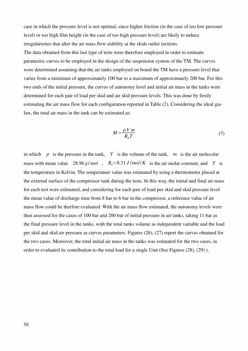
case in which the pressure level is not optimal, since higher friction (in the case of too low pressure
level) or too high film height (in the case of too high pressure level) are likely to induce
irregularieties that alter the air mass flow stability at the skids outlet sections.
The data obtained from this last type of tests were therefore employed in order to estimate
parametric curves to be employed in the design of the suspension system of the TM. The curves
were determined assuming that the air tanks employed on board the TM have a pressure level that
varies from a minimum of approximately 100 bar to a maximum of approximately 200 bar. For this
two ends of the initial pressure, the curves of autonomy level and initial air mass in the tanks were
determined for each pair of load per skid and air skid pressure levels. This was done by firstly
estimating the air mass flow for each configuration reported in Table (2). Considering the ideal gas
law, the total air mass in the tank can be estimated as:
M=p V m
R0T (7)
in which p is the pressure in the tank, V is the volume of the tank, m is the air molecolar
mass with mean value 28.96 g /mol , R0=8.31 J /mol /K is the air molar constant, and T is
the temperature in Kelvin. The temperature value was estimated by using a thermometer placed at
the external surface of the compressor tank during the tests. In this way, the initial and final air mass
for each test were estimated, and considering for each pair of load per skid and skid pressure level
the mean value of discharge time from 8 bar to 6 bar in the compressor, a reference value of air
mass flow could be therfore evaluated. With the air mass flow estimated, the autonomy levels were
then assessed for the cases of 100 bar and 200 bar of initial pressure in air tanks, taking 11 bar as
the final pressure level in the tanks, with the total tanks volume as independent variable and the load
per skid and skid air pressure as curves parameters. Figures (26), (27) report the curves obtained for
the two cases. Moreover, the total initial air mass in the tanks was estimated for the two cases, in
order to evaluated its contribution to the total load for a single Unit (See Figures (28), (29) ).
58
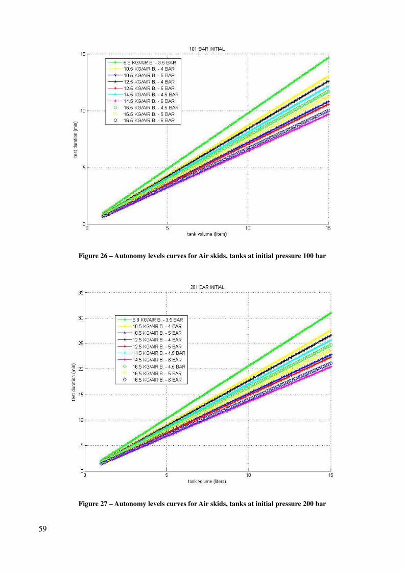
Figure 26 – Autonomy levels curves for Air skids, tanks at initial pressure 100 bar
Figure 27 – Autonomy levels curves for Air skids, tanks at initial pressure 200 bar
59
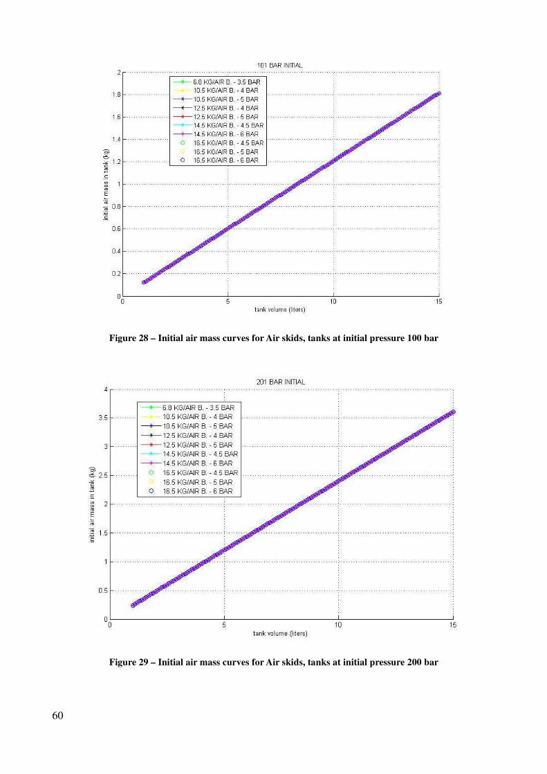
Figure 28 – Initial air mass curves for Air skids, tanks at initial pressure 100 bar
Figure 29 – Initial air mass curves for Air skids, tanks at initial pressure 200 bar
60
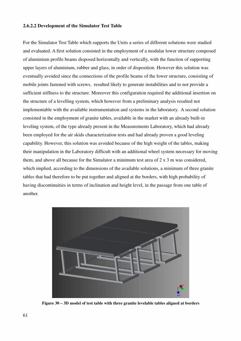
2.6.2.2 Development of the Simulator Test Table
For the Simulator Test Table which supports the Units a series of different solutions were studied
and evaluated. A first solution consisted in the employment of a modular lower structure composed
of aluminium profile beams disposed horizontally and vertically, with the function of supporting
upper layers of aluminium, rubber and glass, in order of disposition. However this solution was
eventually avoided since the connections of the profile beams of the lower structure, consisting of
mobile joints fastened with screws, resulted likely to generate instabilities and to not provide a
sufficient stiffness to the structure. Moreover this configuration required the additional insertion on
the structure of a levelling system, which however from a preliminary analysis resulted not
implementable with the available instrumentation and systems in the laboratory. A second solution
consisted in the employment of granite tables, available in the market with an already built-in
leveling system, of the type already present in the Measurements Laboratory, which had already
been employed for the air skids characterization tests and had already proven a good leveling
capability. However, this solution was avoided because of the high weight of the tables, making
their manipulation in the Laboratory difficult with an additional wheel system necessary for moving
them, and above all because for the Simulator a minimum test area of 2 x 3 m was considered,
which implied, according to the dimensions of the available solutions, a minimum of three granite
tables that had therefore to be put together and aligned at the borders, with high probability of
having discontinuities in terms of inclination and height level, in the passage from one table of
another.
Figure 30 – 3D model of test table with three granite levelable tables aligned at borders
61
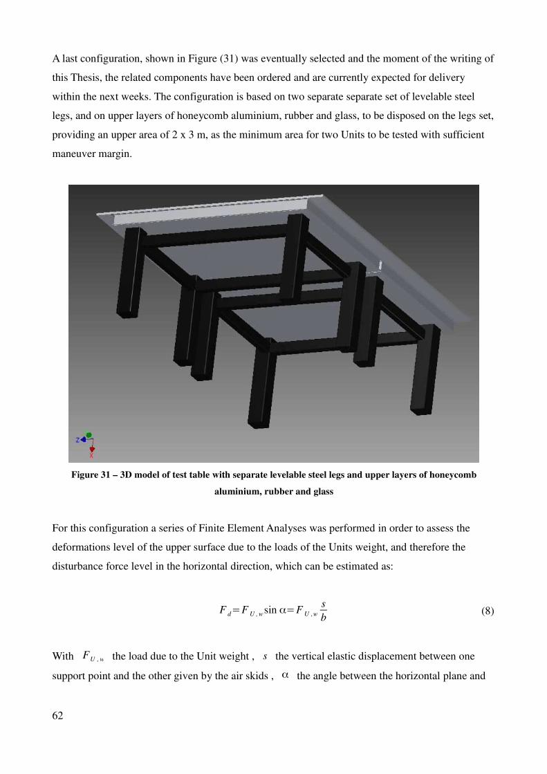
A last configuration, shown in Figure (31) was eventually selected and the moment of the writing of
this Thesis, the related components have been ordered and are currently expected for delivery
within the next weeks. The configuration is based on two separate separate set of levelable steel
legs, and on upper layers of honeycomb aluminium, rubber and glass, to be disposed on the legs set,
providing an upper area of 2 x 3 m, as the minimum area for two Units to be tested with sufficient
maneuver margin.
Figure 31 – 3D model of test table with separate levelable steel legs and upper layers of honeycomb
aluminium, rubber and glass
For this configuration a series of Finite Element Analyses was performed in order to assess the
deformations level of the upper surface due to the loads of the Units weight, and therefore the
disturbance force level in the horizontal direction, which can be estimated as:
F d=F U , w sin α=F U ,w
s
b (8)
With FU , w the load due to the Unit weight , s the vertical elastic displacement between one
support point and the other given by the air skids , α the angle between the horizontal plane and
62
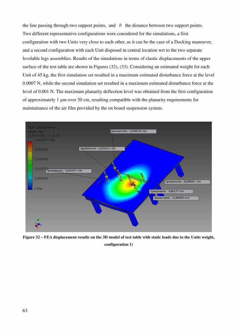
the line passing through two support points, and b the distance between two support points.
Two different representative configurations were considered for the simulations, a first
configuration with two Units very close to each other, as it can be the case of a Docking maneuver,
and a second configuration with each Unit disposed in central location wrt to the two separate
levelable legs assemblies. Results of the simulations in terms of elastic displacements of the upper
surface of the test table are shown in Figures (32), (33). Considering an estimated weight for each
Unit of 45 kg, the first simulation set resulted in a maximum estimated disturbance force at the level
0.0007 N, while the second simulation set resulted in a maximum estimated disturbance force at the
level of 0.001 N. The maximum planarity deflection level was obtained from the first configuration
of approximately 1 μm over 30 cm, resulting compatible with the planarity requirements for
maintainance of the air film provided by the on board suspension system.
Figure 32 – FEA displacement results on the 3D model of test table with static loads due to the Units weight,
configuration 1)
63
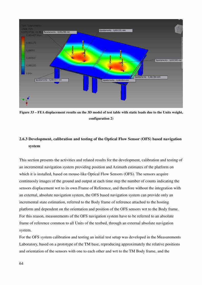
Figure 33 – FEA displacement results on the 3D model of test table with static loads due to the Units weight,
configuration 2)
2.6.3 Development, calibration and testing of the Optical Flow Sensor (OFS) based navigation
system
This section presents the activities and related results for the development, calibration and testing of
an incremental navigation system providing position and Azimuth estimates of the platform on
which it is installed, based on mouse-like Optical Flow Sensors (OFS). The sensors acquire
continuosly images of the ground and output at each time step the number of counts indicating the
sensors displacement wrt to its own Frame of Reference, and therefore without the integration with
an external, absolute navigation system, the OFS based navigation system can provide only an
incremental state estimation, referred to the Body frame of reference attached to the hosting
platform and dependent on the orientation and position of the OFS sensors wrt to the Body frame.
For this reason, measurements of the OFS navigation system have to be referred to an absolute
frame of reference common to all Units of the testbed, through an external absolute navigation
system.
For the OFS system calibration and testing an initial test setup was developed in the Measurements
Laboratory, based on a prototype of the TM base, reproducing approximately the relative positions
and orientation of the sensors with one to each other and wrt to the TM Body frame, and the
64
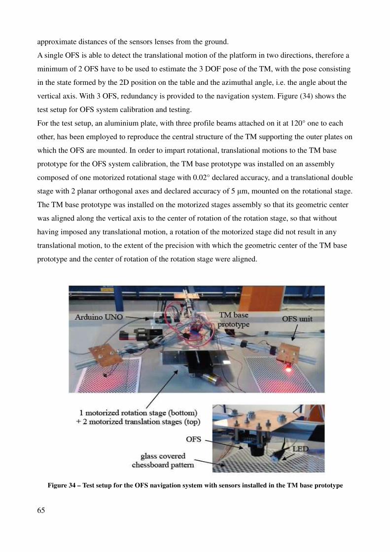
approximate distances of the sensors lenses from the ground.
A single OFS is able to detect the translational motion of the platform in two directions, therefore a
minimum of 2 OFS have to be used to estimate the 3 DOF pose of the TM, with the pose consisting
in the state formed by the 2D position on the table and the azimuthal angle, i.e. the angle about the
vertical axis. With 3 OFS, redundancy is provided to the navigation system. Figure (34) shows the
test setup for OFS system calibration and testing.
For the test setup, an aluminium plate, with three profile beams attached on it at 120° one to each
other, has been employed to reproduce the central structure of the TM supporting the outer plates on
which the OFS are mounted. In order to impart rotational, translational motions to the TM base
prototype for the OFS system calibration, the TM base prototype was installed on an assembly
composed of one motorized rotational stage with 0.02° declared accuracy, and a translational double
stage with 2 planar orthogonal axes and declared accuracy of 5 μm, mounted on the rotational stage.
The TM base prototype was installed on the motorized stages assembly so that its geometric center
was aligned along the vertical axis to the center of rotation of the rotation stage, so that without
having imposed any translational motion, a rotation of the motorized stage did not result in any
translational motion, to the extent of the precision with which the geometric center of the TM base
prototype and the center of rotation of the rotation stage were aligned.
Figure 34 – Test setup for the OFS navigation system with sensors installed in the TM base prototype
65
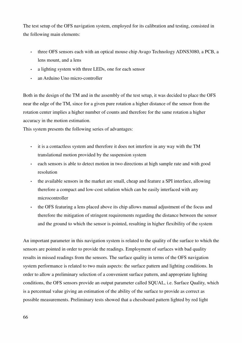
The test setup of the OFS navigation system, employed for its calibration and testing, consisted in
the following main elements:
• three OFS sensors each with an optical mouse chip Avago Technology ADNS3080, a PCB, a
lens mount, and a lens
• a lighting system with three LEDs, one for each sensor
• an Arduino Uno micro-controller
Both in the design of the TM and in the assembly of the test setup, it was decided to place the OFS
near the edge of the TM, since for a given pure rotation a higher distance of the sensor from the
rotation center implies a higher number of counts and therefore for the same rotation a higher
accuracy in the motion estimation.
This system presents the following series of advantages:
• it is a contactless system and therefore it does not interfere in any way with the TM
translational motion provided by the suspension system
• each sensors is able to detect motion in two directions at high sample rate and with good
resolution
• the available sensors in the market are small, cheap and feature a SPI interface, allowing
therefore a compact and low-cost solution which can be easily interfaced with any
microcontroller
• the OFS featuring a lens placed above its chip allows manual adjustment of the focus and
therefore the mitigation of stringent requirements regarding the distance between the sensor
and the ground to which the sensor is pointed, resulting in higher flexibility of the system
An important parameter in this navigation system is related to the quality of the surface to which the
sensors are pointed in order to provide the readings. Employment of surfaces with bad quality
results in missed readings from the sensors. The surface quality in terms of the OFS navigation
system performance is related to two main aspects: the surface pattern and lighting conditions. In
order to allow a preliminary selection of a convenient surface pattern, and appropriate lighting
conditions, the OFS sensors provide an output parameter called SQUAL, i.e. Surface Quality, which
is a percentual value giving an estimation of the ability of the surface to provide as correct as
possible measurements. Preliminary tests showed that a chessboard pattern lighted by red light
66
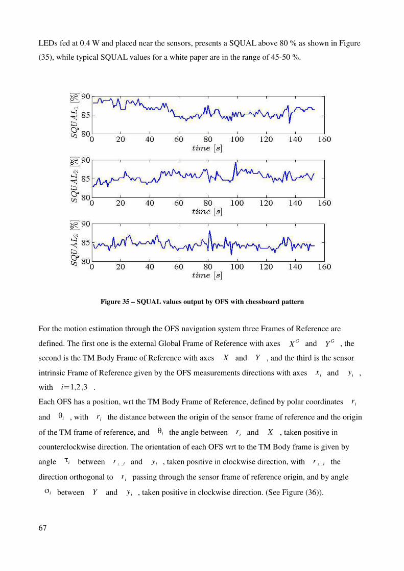
LEDs fed at 0.4 W and placed near the sensors, presents a SQUAL above 80 % as shown in Figure
(35), while typical SQUAL values for a white paper are in the range of 45-50 %.
Figure 35 – SQUAL values output by OFS with chessboard pattern
For the motion estimation through the OFS navigation system three Frames of Reference are
defined. The first one is the external Global Frame of Reference with axes XG and Y
G , the
second is the TM Body Frame of Reference with axes X and Y , and the third is the sensor
intrinsic Frame of Reference given by the OFS measurements directions with axes x i and yi ,
with i=1,2 ,3 .
Each OFS has a position, wrt the TM Body Frame of Reference, defined by polar coordinates r i
and θi , with ri the distance between the origin of the sensor frame of reference and the origin
of the TM frame of reference, and θi the angle between r i and X , taken positive in
counterclockwise direction. The orientation of each OFS wrt to the TM Body frame is given by
angle τi between r⊥ ,i and yi , taken positive in clockwise direction, with r
⊥ ,i the
direction orthogonal to r i passing through the sensor frame of reference origin, and by angle
σi between Y and yi , taken positive in clockwise direction. (See Figure (36)).
67
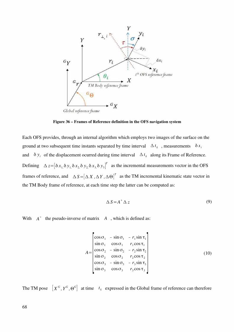
Figure 36 – Frames of Reference definition in the OFS navigation system
Each OFS provides, through an internal algorithm which employs two images of the surface on the
ground at two subsequent time instants separated by time interval ∆ t k , measurements δ x i
and δ y i of the displacement ocurred during time interval ∆ t k along its Frame of Reference.
Defining ∆ z=[δ x1,δ y1,δ x2,δ y2,δ x3,δ y3 ]T
as the incremental measurements vector in the OFS
frames of reference, and ∆ S=[∆ X ,∆Y ,∆Θ ]T
as the TM incremental kinematic state vector in
the TM Body frame of reference, at each time step the latter can be computed as:
∆ S=A+∆ z (9)
With A+ the pseudo-inverse of matrix A , which is defined as:
A=[cosσ1 − sinσ1 − r1 sin τ1
sinσ1 cosσ1 r1 cos τ1
cosσ2 − sinσ2 − r2 sin τ2
sinσ2 cosσ2 r2 cos τ2
cosσ3 − sinσ3 − r3 sin τ3
sinσ3 cosσ3 r3 cos τ3
] (10)
The TM pose [X G, Y
G,ΘG ] at time t k expressed in the Global frame of reference can therefore
68
be computed through the TM pose at the previous time step t k− 1 and the incremental kinematic
state vector [∆ X k ,∆Y k ,∆Θk ] as follows:
X k
G=X k− 1
G +∆ X k cos (Θk− 1)− ∆Y k sin (Θk − 1 ) (11)
Y k
G=Y k− 1
G +∆ X k sin (Θk− 1 )+∆ Y k cos (Θk− 1 ) (12)
Θk
G=Θk− 1
G +∆Θk (13)
With an initial estimate of the TM pose provided, the TM position and orientation can be updated at
each time step t k through the OFS measurements and equations (11), (12), (13). For the real time
TM motion estimation, these equations are implemented in the microcontroller on board the
platform.
2.6.3.1 Calbration of the OFS navigation system
The estimation of the TM pose through the OFS measurements implies the need to know in advance
the values for each sensor of the parameters contained in matrix A , i.e. the position parameters
r i , θi , the orientation parameters τi , σi and the sensitivity k i of each OFS wrt to the
TM Body frame of reference. These parameters have been estimated through the OFS system
calibration performed in accordance to the procedure proposed by Bonarini et al. in [13]. In order to
reduce systematic errors, a refinement calibration based on an optimization procedure with the
available data was subsequently performed.
The calibration is performed through the imposition to the TM prototype of known translational and
rotational motions, through the motorized stages assembly described in the previous section. The
calibration consists in two main phases: a first translational phase, and a second rotational phase.
The translational phase foresees the imposition on the TM of several predetermined linear
displacements ∆ X , ∆Y , simultaneously recording the three OFS raw displacements
(counts) δ x , δ y that are output by the sensor during the motion. For each imposed
translational displacement, the sensor sensitivity k i , i.e. the ratio between metric and raw
displacement, and the sensor orientation σi are estimated respectively as:
69
k i=√∆ X
2+∆Y2
√δ x i
2+δ yi
2 (14)
σi=tan− 1(∆ X
∆ Y )− tan− 1(δ x i
δ y i) (15)
For the translational calibration phase, Table (3) reports the imposed translational motions, while
Figures (37), (38) report the results in terms of sensitivity k and orientation angle σ . Table (4)
reports the mean values of k i and σi for all OFS over the 22 performed tests, taken as best
estimations of the parameters.
For the rotational calibration phase, a series of known rotations ∆Θ about the TM z axis of the
Body frame of reference are imposed with simultaneous acquisition of the sensors measurements,
providing the raw readings δ x i , j , δ y i , j for each rotation step at each jth sampling instant.
In this way the distance r i and orientation τi can be computed as:
r i=k i
∑jδ l i , j
∆Θ =k i
∑j√δ xi , j
2 +δ y i , j
2
∆Θ (16)
τi=tan− 1(δ x i
δ y i) (17)
Imposed rotational motions during the calibration phase are reported in Table (3), Figures (39), (40)
report the results of distance and orientation, while Table (4) reports their mean values together with
the estimated value for θi=τi− σi .
Test number
Translational phase Rotational phase
∆ X [mm] ∆Y [mm] ∆Θ [deg ]
1 0 20 2
2 0 10 2
3 -20 0 2
4 0 -10 2
5 0 10 2
70
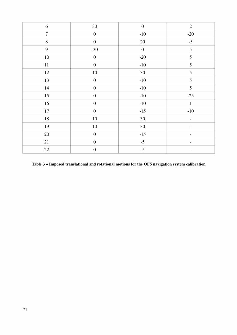
6 30 0 2
7 0 -10 -20
8 0 20 -5
9 -30 0 5
10 0 -20 5
11 0 -10 5
12 10 30 5
13 0 -10 5
14 0 -10 5
15 0 -10 -25
16 0 -10 1
17 0 -15 -10
18 10 30 -
19 10 30 -
20 0 -15 -
21 0 -5 -
22 0 -5 -
Table 3 – Imposed translational and rotational motions for the OFS navigation system calibration
71
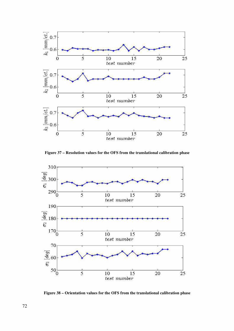
Figure 37 – Resolution values for the OFS from the translational calibration phase
Figure 38 – Orientation values for the OFS from the translational calibration phase
72
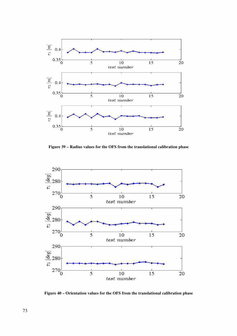
Figure 39 – Radius values for the OFS from the translational calibration phase
Figure 40 – Orientation values for the OFS from the translational calibration phase
73
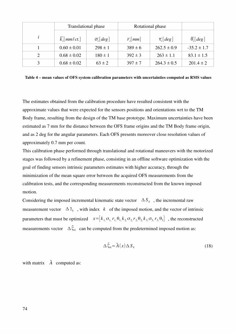
i
Translational phase Rotational phase
k i[mm /ct.] σi [deg ] r i[mm] τi [deg ] θi [deg ]
1 0.60 ± 0.01 298 ± 1 389 ± 6 262.5 ± 0.9 -35.2 ± 1.7
2 0.68 ± 0.02 180 ± 1 392 ± 3 263 ± 1.1 83.1 ± 1.5
3 0.68 ± 0.02 63 ± 2 397 ± 7 264.3 ± 0.5 201.4 ± 2
Table 4 – mean values of OFS system calibration parameters with uncertainties computed as RMS values
The estimates obtained from the calibration procedure have resulted consistent with the
approximate values that were expected for the sensors positions and orientations wrt to the TM
Body frame, resulting from the design of the TM base prototype. Maximum uncertainties have been
estimated as 7 mm for the distance between the OFS frame origins and the TM Body frame origin,
and as 2 deg for the angular parameters. Each OFS presents moreover close resolution values of
approximately 0.7 mm per count.
This calibration phase performed through translational and rotational maneuvers with the motorized
stages was followed by a refinement phase, consisting in an offline software optimization with the
goal of finding sensors intrinsic parameters estimates with higher accuracy, through the
minimization of the mean square error between the acquired OFS measurements from the
calibration tests, and the corresponding measurements reconstructed from the known imposed
motion.
Considering the imposed incremental kinematic state vector ∆ S k , the incremental raw
measurement vector ∆ zk , with index k of the imposed motion, and the vector of intrinsic
parameters that must be optimized x=[k 1,σ1, r1,θ1, k 2,σ2, r 2,θ2, k 3,σ3, r3,θ3 ] , the reconstructed
measurements vector ∆ ζk can be computed from the predetermined imposed motion as:
∆ ζk= A(x)∆ S k (18)
with matrix A computed as:
74
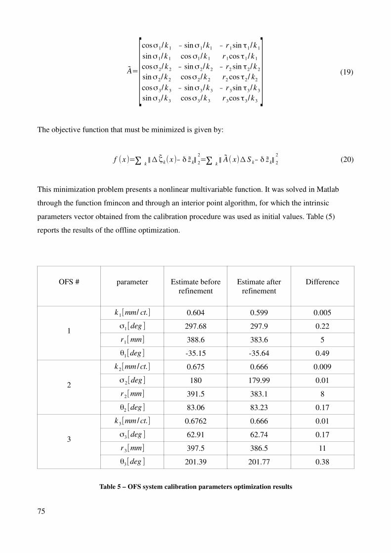
A=[cosσ1/k 1 − sinσ1/k1 − r 1sin τ1/k 1
sinσ1/k 1 cosσ1/k 1 r 1cos τ1/k 1
cosσ2/k 2 − sinσ2/k 2 − r2 sin τ2/k 2
sinσ2/k 2 cosσ2/k 2 r2 cos τ2/ k2
cosσ3/k 3 − sinσ3/k 3 − r 3sin τ3/k 3
sinσ3/k 3 cosσ3/k 3 r 3cos τ3/k 3
] (19)
The objective function that must be minimized is given by:
f (x )=∑k∥∆ ζk (x )− δ z k∥ 2
2
=∑k∥ A( x)∆ S k− δ z k∥ 2
2
(20)
This minimization problem presents a nonlinear multivariable function. It was solved in Matlab
through the function fmincon and through an interior point algorithm, for which the intrinsic
parameters vector obtained from the calibration procedure was used as initial values. Table (5)
reports the results of the offline optimization.
OFS # parameter Estimate before
refinement
Estimate after
refinement
Difference
1
k 1[mm/ ct.] 0.604 0.599 0.005
σ1[deg ] 297.68 297.9 0.22
r1[mm] 388.6 383.6 5
θ1[deg ] -35.15 -35.64 0.49
2
k 2[mm /ct.] 0.675 0.666 0.009
σ2[deg ] 180 179.99 0.01
r 2[mm] 391.5 383.1 8
θ2 [deg ] 83.06 83.23 0.17
3
k 3[mm /ct.] 0.6762 0.666 0.01
σ3[deg ] 62.91 62.74 0.17
r 3[mm] 397.5 386.5 11
θ3[deg ] 201.39 201.77 0.38
Table 5 – OFS system calibration parameters optimization results
75
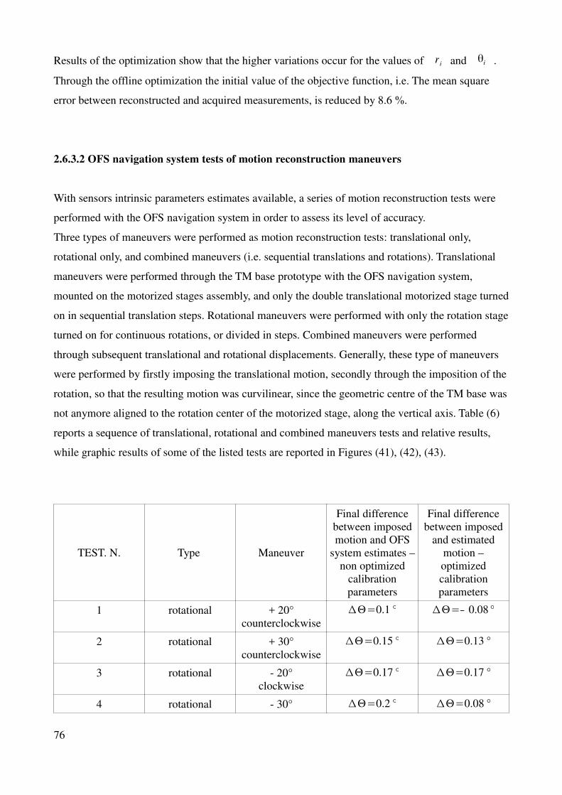
Results of the optimization show that the higher variations occur for the values of r i and θi .
Through the offline optimization the initial value of the objective function, i.e. The mean square
error between reconstructed and acquired measurements, is reduced by 8.6 %.
2.6.3.2 OFS navigation system tests of motion reconstruction maneuvers
With sensors intrinsic parameters estimates available, a series of motion reconstruction tests were
performed with the OFS navigation system in order to assess its level of accuracy.
Three types of maneuvers were performed as motion reconstruction tests: translational only,
rotational only, and combined maneuvers (i.e. sequential translations and rotations). Translational
maneuvers were performed through the TM base prototype with the OFS navigation system,
mounted on the motorized stages assembly, and only the double translational motorized stage turned
on in sequential translation steps. Rotational maneuvers were performed with only the rotation stage
turned on for continuous rotations, or divided in steps. Combined maneuvers were performed
through subsequent translational and rotational displacements. Generally, these type of maneuvers
were performed by firstly imposing the translational motion, secondly through the imposition of the
rotation, so that the resulting motion was curvilinear, since the geometric centre of the TM base was
not anymore aligned to the rotation center of the motorized stage, along the vertical axis. Table (6)
reports a sequence of translational, rotational and combined maneuvers tests and relative results,
while graphic results of some of the listed tests are reported in Figures (41), (42), (43).
TEST. N. Type Maneuver
Final difference
between imposed
motion and OFS
system estimates –
non optimized
calibration
parameters
Final difference
between imposed
and estimated
motion –
optimized
calibration
parameters
1 rotational + 20°
counterclockwise
∆Θ=0.1 ° ∆Θ=− 0.08°
2 rotational + 30°
counterclockwise
∆Θ=0.15 ° ∆Θ=0.13 °
3 rotational - 20°
clockwise
∆Θ=0.17 ° ∆Θ=0.17 °
4 rotational - 30° ∆Θ=0.2 ° ∆Θ=0.08 °
76
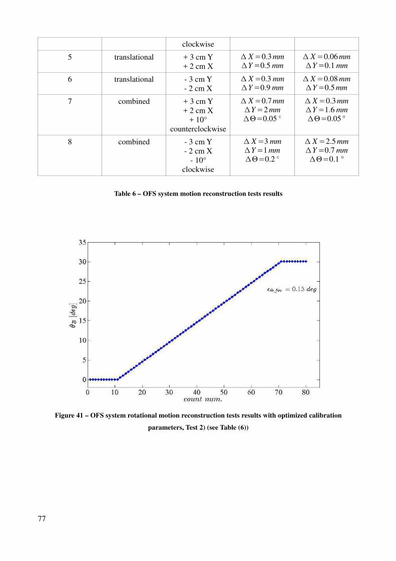
clockwise
5 translational + 3 cm Y
+ 2 cm X
∆ X=0.3mm∆Y=0.5 mm
∆ X=0.06mm∆Y=0.1 mm
6 translational - 3 cm Y
- 2 cm X
∆ X=0.3 mm∆Y=0.9 mm
∆ X=0.08 mm∆Y=0.5 mm
7 combined + 3 cm Y
+ 2 cm X
+ 10°
counterclockwise
∆ X=0.7 mm∆Y=2mm∆Θ=0.05 °
∆ X=0.3mm∆Y=1.6 mm∆Θ=0.05°
8 combined - 3 cm Y
- 2 cm X
- 10°
clockwise
∆ X=3 mm∆Y=1 mm∆Θ=0.2 °
∆ X=2.5 mm∆Y=0.7 mm∆Θ=0.1 °
Table 6 – OFS system motion reconstruction tests results
Figure 41 – OFS system rotational motion reconstruction tests results with optimized calibration
parameters, Test 2) (see Table (6))
77
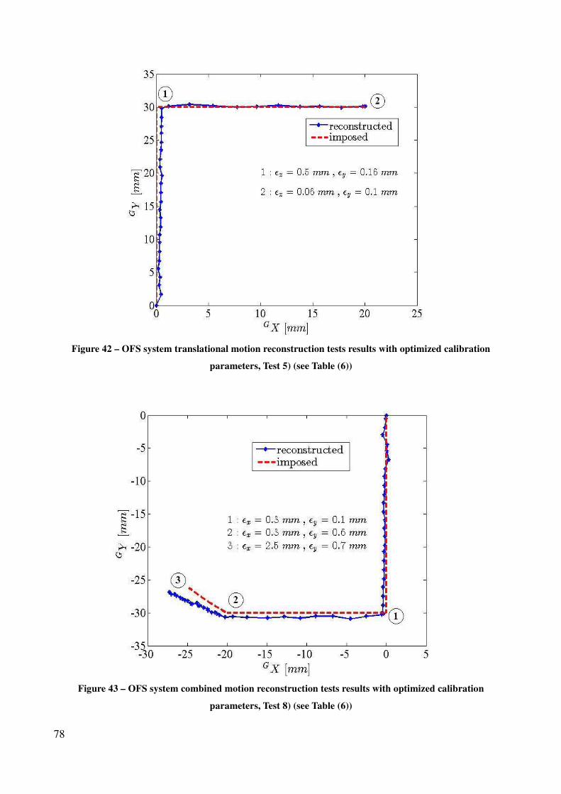
Figure 42 – OFS system translational motion reconstruction tests results with optimized calibration
parameters, Test 5) (see Table (6))
Figure 43 – OFS system combined motion reconstruction tests results with optimized calibration
parameters, Test 8) (see Table (6))
78
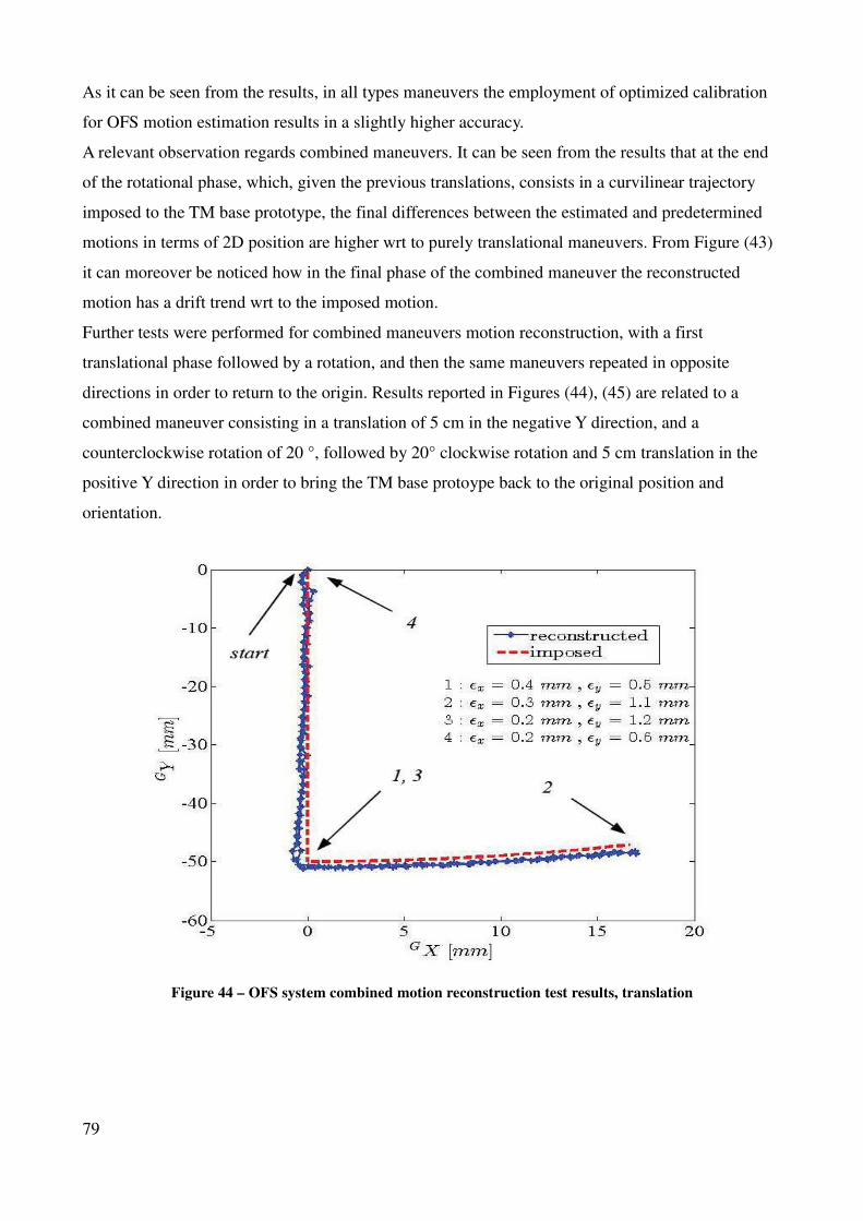
As it can be seen from the results, in all types maneuvers the employment of optimized calibration
for OFS motion estimation results in a slightly higher accuracy.
A relevant observation regards combined maneuvers. It can be seen from the results that at the end
of the rotational phase, which, given the previous translations, consists in a curvilinear trajectory
imposed to the TM base prototype, the final differences between the estimated and predetermined
motions in terms of 2D position are higher wrt to purely translational maneuvers. From Figure (43)
it can moreover be noticed how in the final phase of the combined maneuver the reconstructed
motion has a drift trend wrt to the imposed motion.
Further tests were performed for combined maneuvers motion reconstruction, with a first
translational phase followed by a rotation, and then the same maneuvers repeated in opposite
directions in order to return to the origin. Results reported in Figures (44), (45) are related to a
combined maneuver consisting in a translation of 5 cm in the negative Y direction, and a
counterclockwise rotation of 20 °, followed by 20° clockwise rotation and 5 cm translation in the
positive Y direction in order to bring the TM base protoype back to the original position and
orientation.
Figure 44 – OFS system combined motion reconstruction test results, translation
79
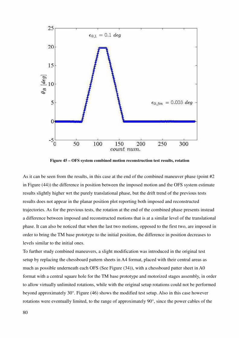
Figure 45 – OFS system combined motion reconstruction test results, rotation
As it can be seen from the results, in this case at the end of the combined maneuver phase (point #2
in Figure (44)) the difference in position between the imposed motion and the OFS system estimate
results slightly higher wrt the purely translational phase, but the drift trend of the previous tests
results does not appear in the planar position plot reporting both imposed and reconstructed
trajectories. As for the previous tests, the rotation at the end of the combined phase presents instead
a difference between imposed and reconstructed motions that is at a similar level of the translational
phase. It can also be noticed that when the last two motions, opposed to the first two, are imposed in
order to bring the TM base prototype to the initial position, the difference in position decreases to
levels similar to the initial ones.
To further study combined maneuvers, a slight modification was introduced in the original test
setup by replacing the chessboard pattern sheets in A4 format, placed with their central areas as
much as possible underneath each OFS (See Figure (34)), with a chessboard patter sheet in A0
format with a central square hole for the TM base prototype and motorized stages assembly, in order
to allow virtually unlimited rotations, while with the original setup rotations could not be performed
beyond approximately 30°. Figure (46) shows the modified test setup. Also in this case however
rotations were eventually limited, to the range of approximately 90°, since the power cables of the
80
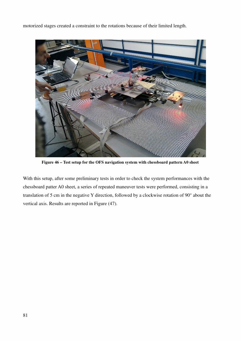
motorized stages created a constraint to the rotations because of their limited length.
Figure 46 – Test setup for the OFS navigation system with chessboard pattern A0 sheet
With this setup, after some preliminary tests in order to check the system performances with the
chessboard patter A0 sheet, a series of repeated maneuver tests were performed, consisting in a
translation of 5 cm in the negative Y direction, followed by a clockwise rotation of 90° about the
vertical axis. Results are reported in Figure (47).
81
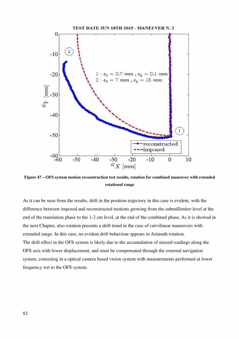
Figure 47 – OFS system motion reconstruction test results, rotation for combined maneuver with extended
rotational range
As it can be seen from the results, drift in the position trajectory in this case is evident, with the
difference between imposed and reconstructed motions growing from the submillimiter level at the
end of the translation phase to the 1-2 cm level, at the end of the combined phase. As it is showed in
the next Chapter, also rotation presents a drift trend in the case of curvilinear maneuvers with
extended range. In this case, no evident drift behaviour appears in Azimuth rotation.
The drift effect in the OFS system is likely due to the accumulation of missed readings along the
OFS axis with lower displacement, and must be compensated through the external navigation
system, consisting in a optical camera based vision system with measurements performed at lower
frequency wrt to the OFS system.
82

83

3 INTEGRATION OF THE OFS NAVIGATION SYSTEM WITH THE VISION SYSTEM
This chapter presents the preliminary activities performed for the integration of the Optical Flow
Sensor (OFS) incremental navigation system with the vision based absolute navigation system for
the pose (planar position and Azimuth) estimation of a 3DOF Unit.
3.1 Integration of the OFS and Vision based Navigation Systems
For the pose estimation of the TM base, the OFS navigation system has been integrated with a
vision based navigation system in order to refer the OFS estimations to an external absolute Frame
of Reference common to all Units, and correct them periodically when their accuracy decreases as
in the cases of curvilinear trajectories, as seen from the results shown in Section 2.6.3.2 in the
previous Chapter. At the moment of the writing of this thesis, the vision system has been employed
for the estimation of the pose of the TM only, but in the next few months with the first complete
Unit assembled, it will be employed also for the estimation of the 3 DOF attitude of the AM,
together with the 2 DOF position of the TM. The final navigation system consists in the vision
based navigation system adopted for low frequency position and attitude estimation in an external
Absolute navigation system, and on board OFS system for high frequency incremental localization.
Morevoer, the vision based navigation system is employed for OFS drift compensation.
The integration of the two navigation systems has been performed with the OFS sensors installed in
the nominal configuration in the TM base, with the TM base preliminary assembled in its main
central structure, as shown in Figure (48), with the OFS sensors at the right distance from the
ground, with styrofoam blocks in order to put the pattern sheets at the right distance. The calibration
procedure presented in section 2.6.3.1 has been repeated in this nominal configuration and related
results are reported in Table (7).
84
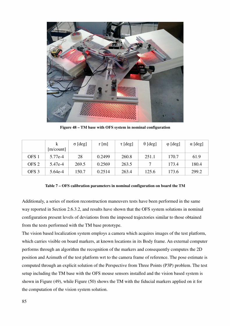
Figure 48 – TM base with OFS system in nominal configuration
k
[m/count]
σ [deg] r [m] τ [deg] θ [deg] φ [deg] α [deg]
OFS 1 5.77e-4 28 0.2499 260.8 251.1 170.7 61.9
OFS 2 5.47e-4 269.5 0.2569 263.5 7 173.4 180.4
OFS 3 5.64e-4 150.7 0.2514 263.4 125.6 173.6 299.2
Table 7 – OFS calibration parameters in nominal configuration on board the TM
Additionaly, a series of motion reconstruction maneuvers tests have been performed in the same
way reported in Section 2.6.3.2, and results have shown that the OFS system solutions in nominal
configuration present levels of deviations from the imposed trajectories similar to those obtained
from the tests performed with the TM base prototype.
The vision based localization system employs a camera which acquires images of the test platform,
which carries visible on board markers, at known locations in its Body frame. An external computer
performs through an algorithm the recognition of the markers and consequently computes the 2D
position and Azimuth of the test platform wrt to the camera frame of reference. The pose estimate is
computed through an explicit solution of the Perspective from Three Points (P3P) problem. The test
setup including the TM base with the OFS mouse sensors installed and the vision based system is
shown in Figure (49), while Figure (50) shows the TM with the fiducial markers applied on it for
the computation of the vision system solution.
85
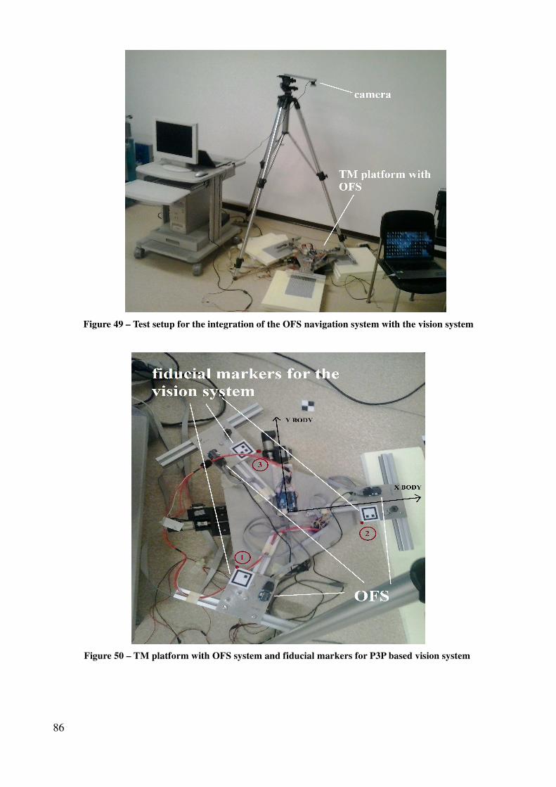
Figure 49 – Test setup for the integration of the OFS navigation system with the vision system
Figure 50 – TM platform with OFS system and fiducial markers for P3P based vision system
86
3.1.1 The Vision based Localization System
In the Vision based localization system a camera, which periodically acquires images of the test
platform with opportune markers on it, is employed as the primary sensor which allows the
resolution of the general problem known as Structure From Motion (SFM), which consists in
recovering relative camera poses and 3D structure from a set of camera images. The SFM problem
includes the problem of 3D reconstruction of the observed structure, and also the estimation of the
relative position and orientation of the camera wrt to the observed scene.
For the application which is presented in this section, this type of system is employed for the
solution of a particular case of the SFM problem. The camera is aimed towards the test platform,
the TM base, which translates and rotates along predetermined trajectories with 3 DOF, two in
planar position and one in rotation (Azimuth), by means of the motorized translation and rotation
stages. Subsequently, a software in an external computer employs the acquired images in order to
evaluate the pose, i.e. the relative position and orientation of the camera wrt to the test platform.
This information can then be used to find in turn the relative pose of the test platform wrt the
camera, i.e. the position and orientation of the TM base expressed in a Frame of Reference attached
to the camera.
For the solution of this problem, the test platform must be set so that it presents a set of points with
known 3D positions in its own frame of reference. If the set of points is within the field of view of
the camera, then also the projections of the 3D points on the acquired images, i.e. the corresponding
2D points on the image plane, are known, and the problem can be solved. This problem is known
for an arbitrary number of points as the Perspective from n Points (PnP) problem, and it presents
many different known solutions, given the following general statement: given a set of m control
points with 3D coordinates, known in a certain coordinate frame, and given an image in which some
subset of the m control points is visible with the camera, determine the location relative to the
coordinate system of the control points from which the image was obtained. In the PnP problem, the
minimum number of points that can be theoretically used to find a solution is three, resulting in
what is known as the P3P problem. It was however found that the employment of three points leads
to determining four equivalent solutions and for this reason a fourth point is necessary for the
elimination of the ambiguity. Neverthless, P3P is an attractive version of the PnP for two main
reasons. Firstly, it presents many direct solutions and secondly its solution can be conveniently
embedded into a RANdom Sample Consensus (RANSAC) scheme, which is an algorithm that
limits the number of outliers, i.e. erroneous associations of the 2D points in the acquired image
plane to 3D control points known in the platform frame of reference.
87
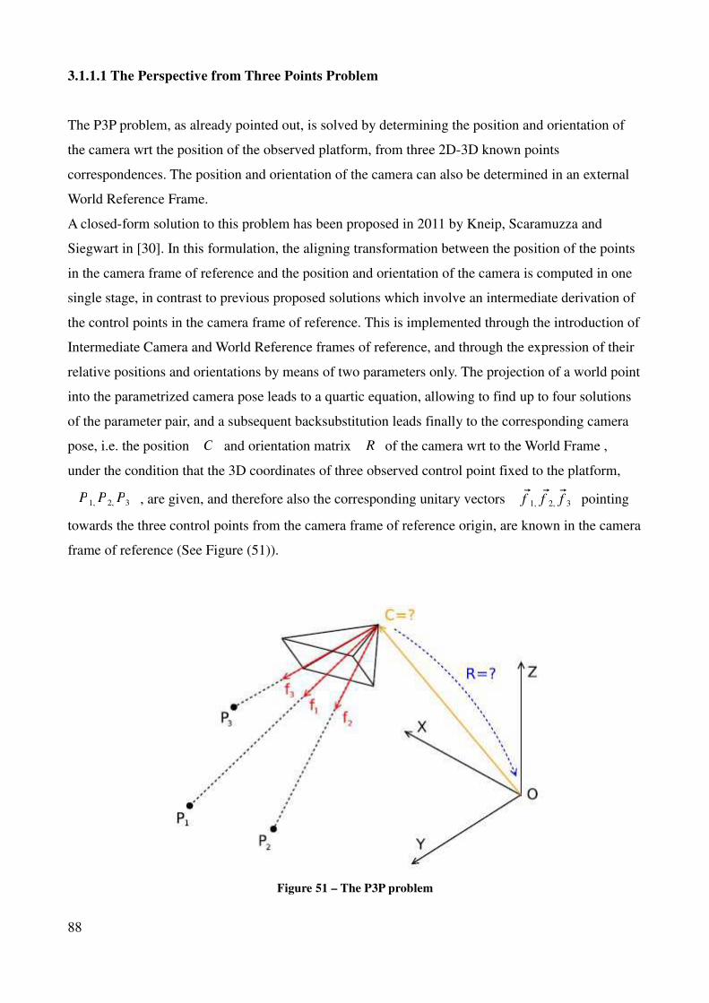
3.1.1.1 The Perspective from Three Points Problem
The P3P problem, as already pointed out, is solved by determining the position and orientation of
the camera wrt the position of the observed platform, from three 2D-3D known points
correspondences. The position and orientation of the camera can also be determined in an external
World Reference Frame.
A closed-form solution to this problem has been proposed in 2011 by Kneip, Scaramuzza and
Siegwart in [30]. In this formulation, the aligning transformation between the position of the points
in the camera frame of reference and the position and orientation of the camera is computed in one
single stage, in contrast to previous proposed solutions which involve an intermediate derivation of
the control points in the camera frame of reference. This is implemented through the introduction of
Intermediate Camera and World Reference frames of reference, and through the expression of their
relative positions and orientations by means of two parameters only. The projection of a world point
into the parametrized camera pose leads to a quartic equation, allowing to find up to four solutions
of the parameter pair, and a subsequent backsubstitution leads finally to the corresponding camera
pose, i.e. the position C and orientation matrix R of the camera wrt to the World Frame ,
under the condition that the 3D coordinates of three observed control point fixed to the platform,
P1, P2, P3 , are given, and therefore also the corresponding unitary vectors f 1, f 2, f 3 pointing
towards the three control points from the camera frame of reference origin, are known in the camera
frame of reference (See Figure (51)).
Figure 51 – The P3P problem
88
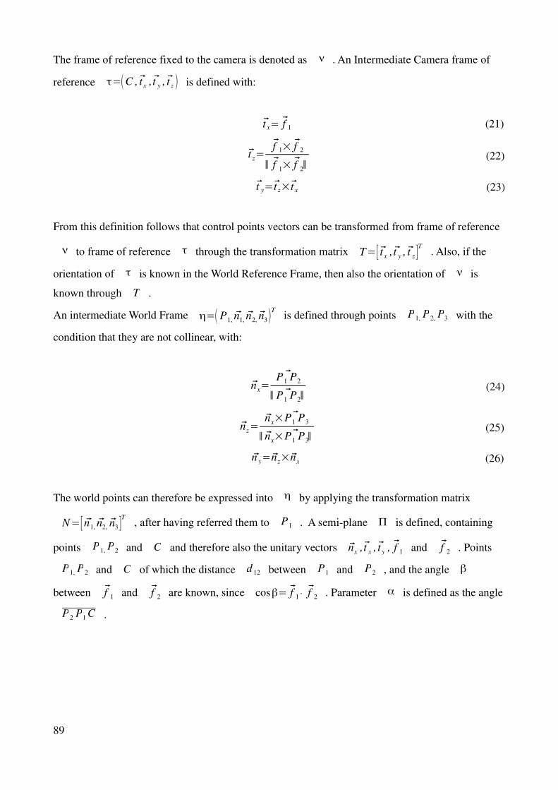
The frame of reference fixed to the camera is denoted as ν . An Intermediate Camera frame of
reference τ=(C , t x , t y , t z ) is defined with:
t x= f 1 (21)
t z=f 1× f 2
∥ f 1× f 2∥ (22)
t y=t z×t x (23)
From this definition follows that control points vectors can be transformed from frame of reference
ν to frame of reference τ through the transformation matrix T=[ t x , t y , t z ]T
. Also, if the
orientation of τ is known in the World Reference Frame, then also the orientation of ν is
known through T .
An intermediate World Frame η=(P1, n1, n2, n3)T
is defined through points P1, P2, P3 with the
condition that they are not collinear, with:
nx=P1 P2
∥ P1 P2∥ (24)
nz=nx× P1 P3
∥ nx× P1 P3∥ (25)
n y=nz×nx (26)
The world points can therefore be expressed into η by applying the transformation matrix
N=[ n1, n2, n3 ]T
, after having referred them to P1 . A semi-plane Π is defined, containing
points P1, P2 and C and therefore also the unitary vectors nx , t x , t y , f 1 and f 2 . Points
P1, P2 and C of which the distance d 12 between P1 and P2 , and the angle β
between f 1 and f 2 are known, since cosβ= f 1 ⋅ f 2 . Parameter α is defined as the angle
P2 P1 C .
89
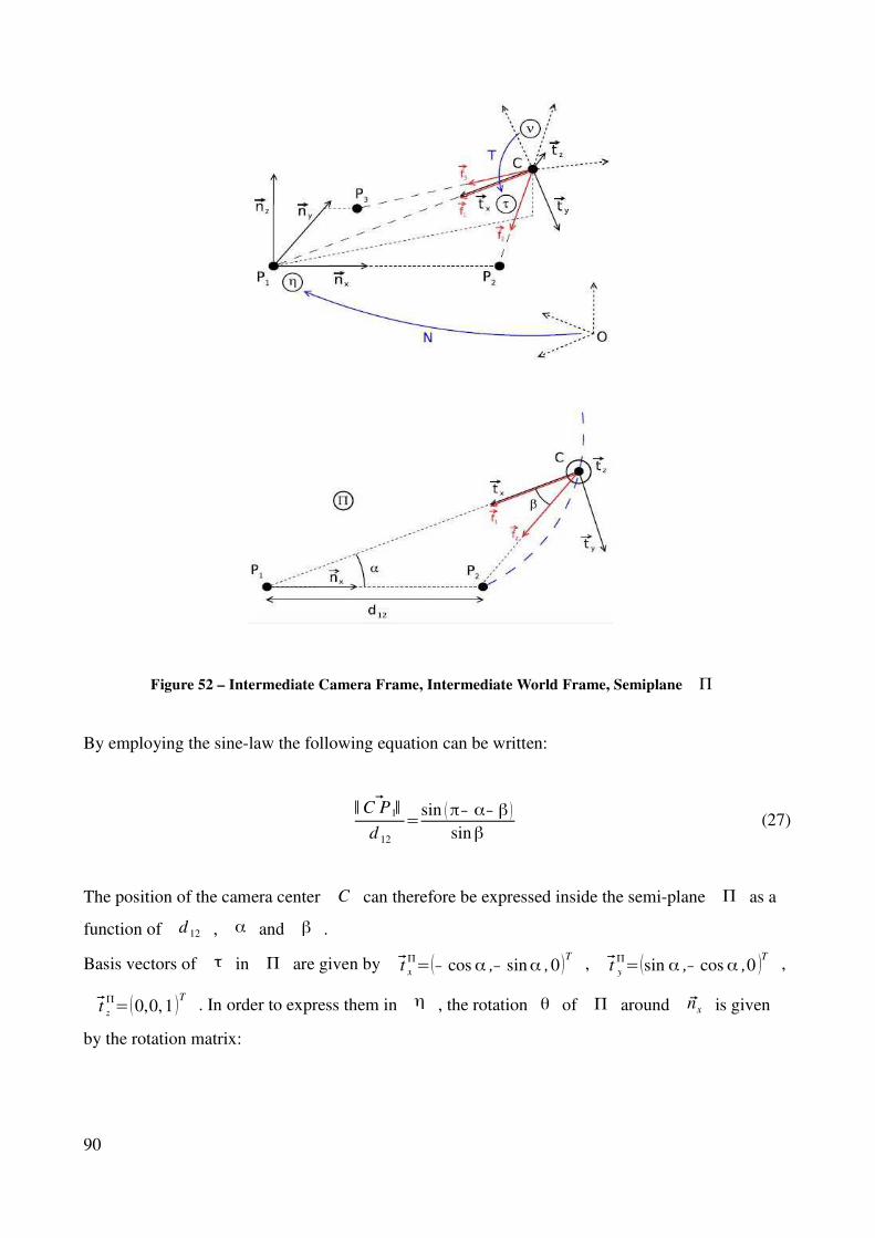
Figure 52 – Intermediate Camera Frame, Intermediate World Frame, Semiplane Π
By employing the sine-law the following equation can be written:
∥ C P1∥
d 12
=sin (π− α− β )
sinβ (27)
The position of the camera center C can therefore be expressed inside the semi-plane Π as a
function of d 12 , α and β .
Basis vectors of τ in Π are given by t x
Π=(− cosα ,− sinα ,0)T
, t y
Π=(sin α ,− cosα ,0 )T
,
t z
Π=(0,0,1)T
. In order to express them in η , the rotation θ of Π around nx is given
by the rotation matrix:
90
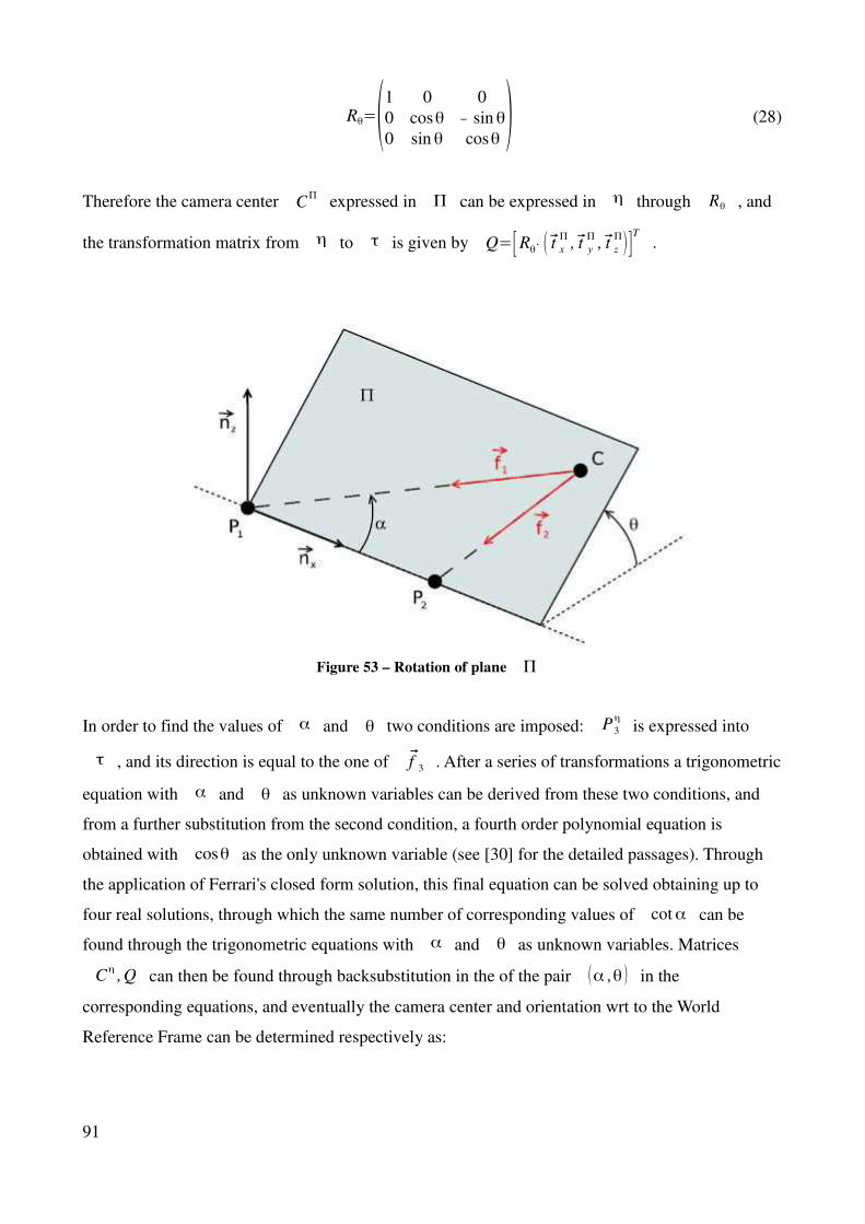
Rθ=(1 0 0
0 cosθ − sinθ0 sinθ cosθ ) (28)
Therefore the camera center CΠ
expressed in Π can be expressed in η through Rθ , and
the transformation matrix from η to τ is given by Q=[Rθ⋅ ( t x
Π, t y
Π, t z
Π)]T
.
Figure 53 – Rotation of plane Π
In order to find the values of α and θ two conditions are imposed: P3
ηis expressed into
τ , and its direction is equal to the one of f 3 . After a series of transformations a trigonometric
equation with α and θ as unknown variables can be derived from these two conditions, and
from a further substitution from the second condition, a fourth order polynomial equation is
obtained with cosθ as the only unknown variable (see [30] for the detailed passages). Through
the application of Ferrari's closed form solution, this final equation can be solved obtaining up to
four real solutions, through which the same number of corresponding values of cotα can be
found through the trigonometric equations with α and θ as unknown variables. Matrices
Cη
,Q can then be found through backsubstitution in the of the pair (α ,θ ) in the
corresponding equations, and eventually the camera center and orientation wrt to the World
Reference Frame can be determined respectively as:
91
C=P1+NT⋅C
η (29)
R=NT⋅Q
T⋅T (30)
Extensive test sessions with this algorithm have shown that it presents accuracy and precision that
are at the level of state-of-the-art approaches to the P3P problem, but at a much lower
computational cost, i.e. approximately 15 times faster. Furthermore the algorithm has proven to be
numerically stable, and to be poorly affected by degenerate configurations of the control points.
Moreover its computational efficiency makes it suitable to be employed with the RANSAC outlier-
rejection algorithm.
3.1.1.2 Measurement Algorithm
The first step of the measurement algorithm of the vision based navigation system consists in the
detection, in each acquired image, of the projections x i
C =[ x i
C, y i
C,1]
Tof the 3D points X i
S
that are attached to the observed platform. The camera, through which the images of the test
platform are acquired, is assumed to be optically calibrated, i.e. all its intrinsic parameters and
optical distorsions are known, therefore the projected points can be expressed in an ideal camera
having the same optical center as the real camera, but an ideal unitary focal length.
The matching phase consists then in associating each detected 2D point x i
Cwith its
corresponding 3D point. The 3D points are initially known only in the test platform frame of
reference S . In order to minimize matching errors between the 3D points and their projections,
opportune fiducial markers are employed. In this activity, markers with a square shape and a known
number of internal dots inside the shape, have been employed. The square shape allows the
detection of the four corners of each marker, in order to facilitate the determination of the marker's
center, while the internal dots allow the identification of the marker, and therefore the retrieval of its
position in the test platform frame of reference, in the phase of matching of the detected 2D points
with the known 3D points. With the 3D points X i
Sand their corresponding projections x i
C
determined, the relative position and orientation between the camera and the platform can be
determined through the explicit solution of the P3P problem presented in the previous section,
inside a RANSAC scheme, and then with a non-linear optimization in order to refine the initial
estimates.
For this particular problem, the output of the employed P3P algorithm consists in four rotation
92
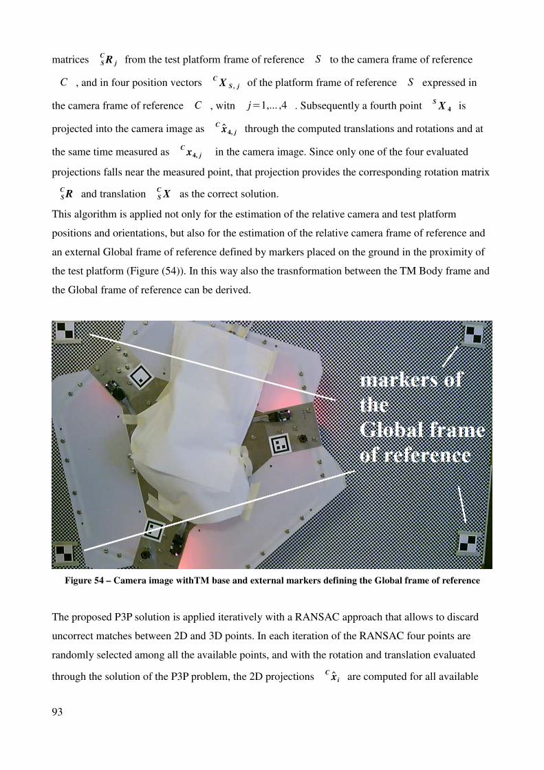
matrices R jS
Cfrom the test platform frame of reference S to the camera frame of reference
C , and in four position vectors X S , j
Cof the platform frame of reference S expressed in
the camera frame of reference C , witn j=1,... ,4 . Subsequently a fourth point X 4
Sis
projected into the camera image as x4, j
Cthrough the computed translations and rotations and at
the same time measured as x4, j
C in the camera image. Since only one of the four evaluated
projections falls near the measured point, that projection provides the corresponding rotation matrix
RS
Cand translation XS
Cas the correct solution.
This algorithm is applied not only for the estimation of the relative camera and test platform
positions and orientations, but also for the estimation of the relative camera frame of reference and
an external Global frame of reference defined by markers placed on the ground in the proximity of
the test platform (Figure (54)). In this way also the trasnformation between the TM Body frame and
the Global frame of reference can be derived.
Figure 54 – Camera image withTM base and external markers defining the Global frame of reference
The proposed P3P solution is applied iteratively with a RANSAC approach that allows to discard
uncorrect matches between 2D and 3D points. In each iteration of the RANSAC four points are
randomly selected among all the available points, and with the rotation and translation evaluated
through the solution of the P3P problem, the 2D projections x i
Care computed for all available
93
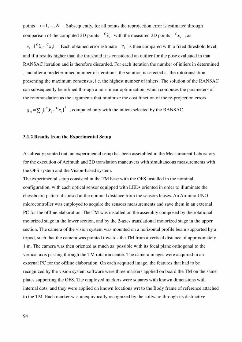
points i=1, ... , N . Subsequently, for all points the reprojection error is estimated through
comparison of the computed 2D points x i
Cwith the measured 2D points x i
C, as
e i=∥ x i
C− x i
C∥ . Each obtained error estimate e i is then compared with a fixed threshold level,
and if it results higher than the threshold it is considered an outlier for the pose evaluated in that
RANSAC iteration and is therefore discarded. For each iteration the number of inliers in determined
, and after a predetermined number of iterations, the solution is selected as the rototranslation
presenting the maximum consensus, i.e. the highest number of inliers. The solution of the RANSAC
can subsequently be refined through a non-linear optimization, which computes the parameters of
the rototranslation as the arguments that minimize the cost function of the re-projection errors
gnl=∑ i∥ x i
C− x i
C∥
2
, computed only with the inliers selected by the RANSAC.
3.1.2 Results from the Experimental Setup
As already pointed out, an experimental setup has been assembled in the Measurement Laboratory
for the execution of Azimuth and 2D translation maneuvers with simultaneous measurements with
the OFS system and the Vision-based system.
The experimental setup consisted in the TM base with the OFS installed in the nominal
configuration, with each optical sensor equipped with LEDs oriented in order to illuminate the
chessboard pattern disposed at the nominal distance from the sensors lenses. An Arduino UNO
microcontroller was employed to acquire the sensors measurements and save them in an external
PC for the offline elaboration. The TM was installed on the assembly composed by the rotational
motorized stage in the lower section, and by the 2-axes translational motorized stage in the upper
section. The camera of the vision system was mounted on a horizontal profile beam supported by a
tripod, such that the camera was pointed towards the TM from a vertical distance of approximately
1 m. The camera was then oriented as much as possible with its focal plane orthogonal to the
vertical axis passing through the TM rotation center. The camera images were acquired in an
external PC for the offline elaboration. On each acquired image, the features that had to be
recognized by the vision system software were three markers applied on board the TM on the same
plates supporting the OFS. The employed markers were squares with known dimensions with
internal dots, and they were applied on known locations wrt to the Body frame of reference attached
to the TM. Each marker was unequivocally recognized by the software through its distinctive
94
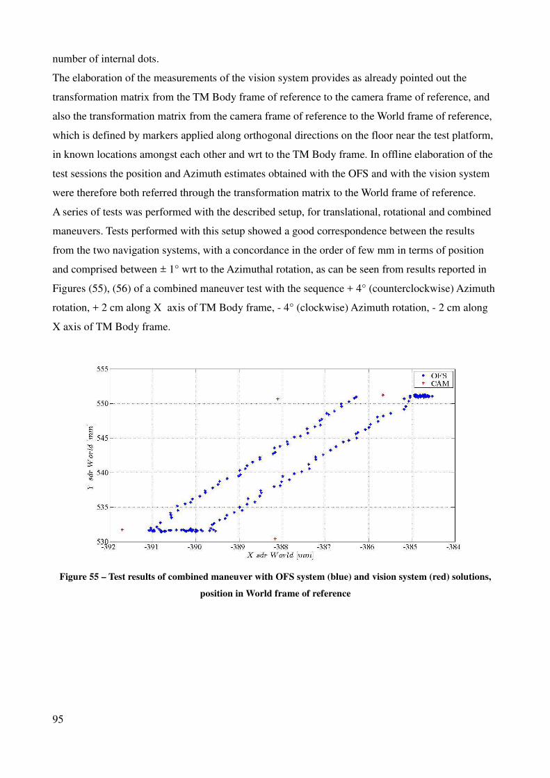
number of internal dots.
The elaboration of the measurements of the vision system provides as already pointed out the
transformation matrix from the TM Body frame of reference to the camera frame of reference, and
also the transformation matrix from the camera frame of reference to the World frame of reference,
which is defined by markers applied along orthogonal directions on the floor near the test platform,
in known locations amongst each other and wrt to the TM Body frame. In offline elaboration of the
test sessions the position and Azimuth estimates obtained with the OFS and with the vision system
were therefore both referred through the transformation matrix to the World frame of reference.
A series of tests was performed with the described setup, for translational, rotational and combined
maneuvers. Tests performed with this setup showed a good correspondence between the results
from the two navigation systems, with a concordance in the order of few mm in terms of position
and comprised between ± 1° wrt to the Azimuthal rotation, as can be seen from results reported in
Figures (55), (56) of a combined maneuver test with the sequence + 4° (counterclockwise) Azimuth
rotation, + 2 cm along X axis of TM Body frame, - 4° (clockwise) Azimuth rotation, - 2 cm along
X axis of TM Body frame.
Figure 55 – Test results of combined maneuver with OFS system (blue) and vision system (red) solutions,
position in World frame of reference
95
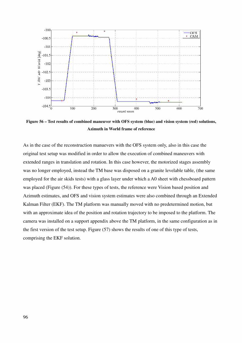
Figure 56 – Test results of combined maneuver with OFS system (blue) and vision system (red) solutions,
Azimuth in World frame of reference
As in the case of the reconstruction manuevers with the OFS system only, also in this case the
original test setup was modified in order to allow the execution of combined maneuvers with
extended ranges in translation and rotation. In this case however, the motorized stages assembly
was no longer employed, instead the TM base was disposed on a granite levelable table, (the same
employed for the air skids tests) with a glass layer under which a A0 sheet with chessboard pattern
was placed (Figure (54)). For these types of tests, the reference were Vision based position and
Azimuth estimates, and OFS and vision system estimates were also combined through an Extended
Kalman Filter (EKF). The TM platform was manually moved with no predetermined motion, but
with an approximate idea of the position and rotation trajectory to be imposed to the platform. The
camera was installed on a support appendix above the TM platform, in the same configuration as in
the first version of the test setup. Figure (57) shows the results of one of this type of tests,
comprising the EKF solution.
96
Figure 57 – Test results of manually imposed combined maneuver with OFS system solution (continuous
blue line)), vision system solution (dotted red line), EKF solution (dashed black line)
As it can be seen from the results, there is a good concordance between the vision based and OFS
system, until the range of combined maneuver is extended. After that, again the OFS system shows
a drift trend, with at the beginning a drift visible only for position, and at the end of the test visible
also for rotation, with final differences at the level of approximately 5 cm in position and of
approximately 35° in Azimuth rotation. The EKF appears able to compensate the drift trend of the
OFS system, since the vision system is considered as fiducial reference, with the EKF uncertainty
output provides max vaules of [σX ,σY ,σΘ]=[7.38mm, 7.38mm ,1.76 deg ] .
97

98
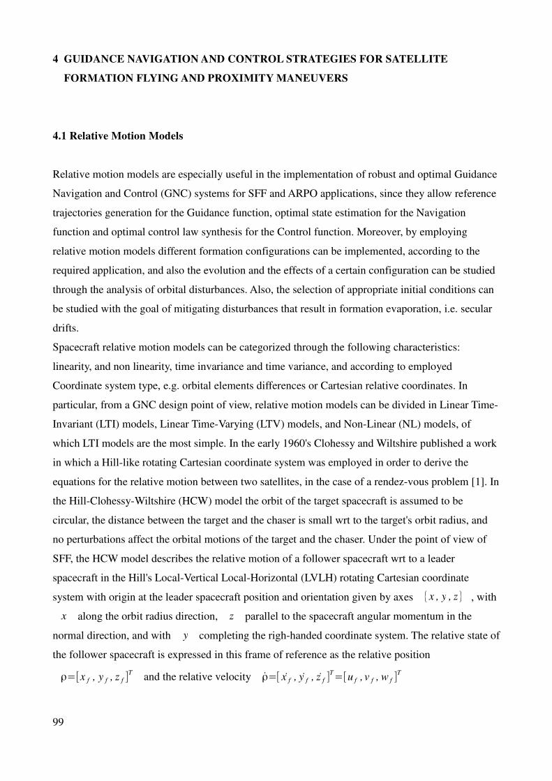
4 GUIDANCE NAVIGATION AND CONTROL STRATEGIES FOR SATELLITE
FORMATION FLYING AND PROXIMITY MANEUVERS
4.1 Relative Motion Models
Relative motion models are especially useful in the implementation of robust and optimal Guidance
Navigation and Control (GNC) systems for SFF and ARPO applications, since they allow reference
trajectories generation for the Guidance function, optimal state estimation for the Navigation
function and optimal control law synthesis for the Control function. Moreover, by employing
relative motion models different formation configurations can be implemented, according to the
required application, and also the evolution and the effects of a certain configuration can be studied
through the analysis of orbital disturbances. Also, the selection of appropriate initial conditions can
be studied with the goal of mitigating disturbances that result in formation evaporation, i.e. secular
drifts.
Spacecraft relative motion models can be categorized through the following characteristics:
linearity, and non linearity, time invariance and time variance, and according to employed
Coordinate system type, e.g. orbital elements differences or Cartesian relative coordinates. In
particular, from a GNC design point of view, relative motion models can be divided in Linear Time-
Invariant (LTI) models, Linear Time-Varying (LTV) models, and Non-Linear (NL) models, of
which LTI models are the most simple. In the early 1960's Clohessy and Wiltshire published a work
in which a Hill-like rotating Cartesian coordinate system was employed in order to derive the
equations for the relative motion between two satellites, in the case of a rendez-vous problem [1]. In
the Hill-Clohessy-Wiltshire (HCW) model the orbit of the target spacecraft is assumed to be
circular, the distance between the target and the chaser is small wrt to the target's orbit radius, and
no perturbations affect the orbital motions of the target and the chaser. Under the point of view of
SFF, the HCW model describes the relative motion of a follower spacecraft wrt to a leader
spacecraft in the Hill's Local-Vertical Local-Horizontal (LVLH) rotating Cartesian coordinate
system with origin at the leader spacecraft position and orientation given by axes x , y , z , with
x along the orbit radius direction, z parallel to the spacecraft angular momentum in the
normal direction, and with y completing the righ-handed coordinate system. The relative state of
the follower spacecraft is expressed in this frame of reference as the relative position
ρ=[x f , y f , z f ]T
and the relative velocity ρ=[ x f , y f , z f ]T=[u f , v f , w f ]
T
99
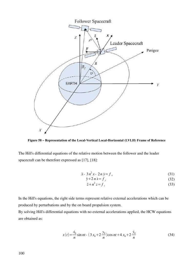
Figure 58 – Representation of the Local-Vertical Local-Horizontal (LVLH) Frame of Reference
The Hill's differential equations of the relative motion between the follower and the leader
spacecraft can be therefore expressed as [17], [18]:
x− 3 n2
x− 2n y= f x (31)
y+2 n x= f y (32)
z+n2z= f z (33)
In the Hill's equations, the right side terms represent relative external accelerations which can be
produced by perturbations and by the on board propulsion system.
By solving Hill's differential equations with no external accelerations applied, the HCW equations
are obtained as:
x (t)=x0
nsin nt− (3 x0+2
y0
n)cos nt+4 x0+2
y0
n (34)
100
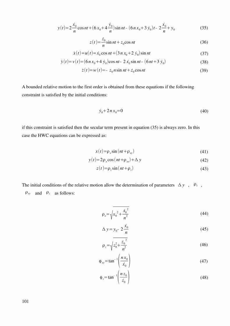
y (t )=2x0
ncosnt+(6 x0+4
y0
n)sin nt− (6n x0+3 y0)t− 2
x0
n+ y0 (35)
z (t )=z0
nsin nt+ z0cos nt (36)
x (t)=u( t )= x0 cos nt+(3 n x0+2 y0)sin nt (37)
y (t )=v (t )=(6n x0+4 y0)cos nt− 2 x0 sin nt− (6nt+3 y0) (38)
z (t )=w (t)=− z0 n sin nt+ z0 cosnt (39)
A bounded relative motion to the first order is obtained from these equations if the following
constraint is satisfied by the initial conditions:
y0+2n x0=0 (40)
if this constraint is satisfied then the secular term present in equation (35) is always zero. In this
case the HWC equations can be expressed as:
x (t)=ρ x sin (nt+ρxy) (41)
y (t )=2ρx cos (nt+ρxy)+∆ y (42)
z (t )=ρz sin(nt+ρz) (43)
The initial conditions of the relative motion allow the determination of parameters ∆ y , ρz ,
ρxy and ρz as follows:
ρx=√x0
2+x0
2
n2
(44)
∆ y= y0− 2x0
n (45)
ρz=√z0
2+z0
2
n2
(46)
ϕxy=tan− 1(n x0
x0) (47)
ϕ z= tan− 1(n z0
z0) (48)
101
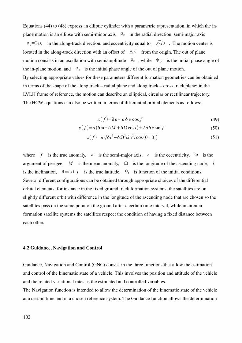
Equations (44) to (48) express an elliptic cylinder with a parametric rapresentation, in which the in-
plane motion is an ellipse with semi-minor axis ρx in the radial direction, semi-major axis
ρ y=2ρx in the along-track direction, and eccentricity equal to √3/2 . The motion center is
located in the along-track direction with an offset of ∆ y from the origin. The out of plane
motion consists in an oscillation with semiamplitude ρz , while ϕxy is the initial phase angle of
the in-plane motion, and ϕ z is the initial phase angle of the out of plane motion.
By selecting appropriate values for these parameters different formation geometries can be obtained
in terms of the shape of the along track – radial plane and along track – cross track plane: in the
LVLH frame of reference, the motion can describe an elliptical, circular or rectilinear trajectory.
The HCW equations can also be written in terms of differential orbital elements as follows:
x ( f )=δa− a δ e cos f (49)
y ( f )=a (δω+δM+δΩcos i)+2aδ e sin f (50)
z ( f )=a √δi2+δΩ2
sin2i cos (θ− θz) (51)
where f is the true anomaly, a is the semi-major axis, e is the eccentricity, ω is the
argument of perigee, M is the mean anomaly, Ω is the longitude of the ascending node, i
is the inclination, θ=ω+ f is the true latitude, θz is function of the initial conditions.
Several different configurations can be obtained through appropriate choices of the differential
orbital elements, for instance in the fixed ground track formation systems, the satellites are on
slightly different orbit with difference in the longitude of the ascending node that are chosen so the
satellites pass on the same point on the ground after a certain time interval, while in circular
formation satellite systems the satellites respect the condition of having a fixed distance between
each other.
4.2 Guidance, Navigation and Control
Guidance, Navigation and Control (GNC) consist in the three functions that allow the estimation
and control of the kinematic state of a vehicle. This involves the position and attitude of the vehicle
and the related variational rates as the estimated and controlled variables.
The Navigation function is intended to allow the determination of the kinematic state of the vehicle
at a certain time and in a chosen reference system. The Guidance function allows the determination
102
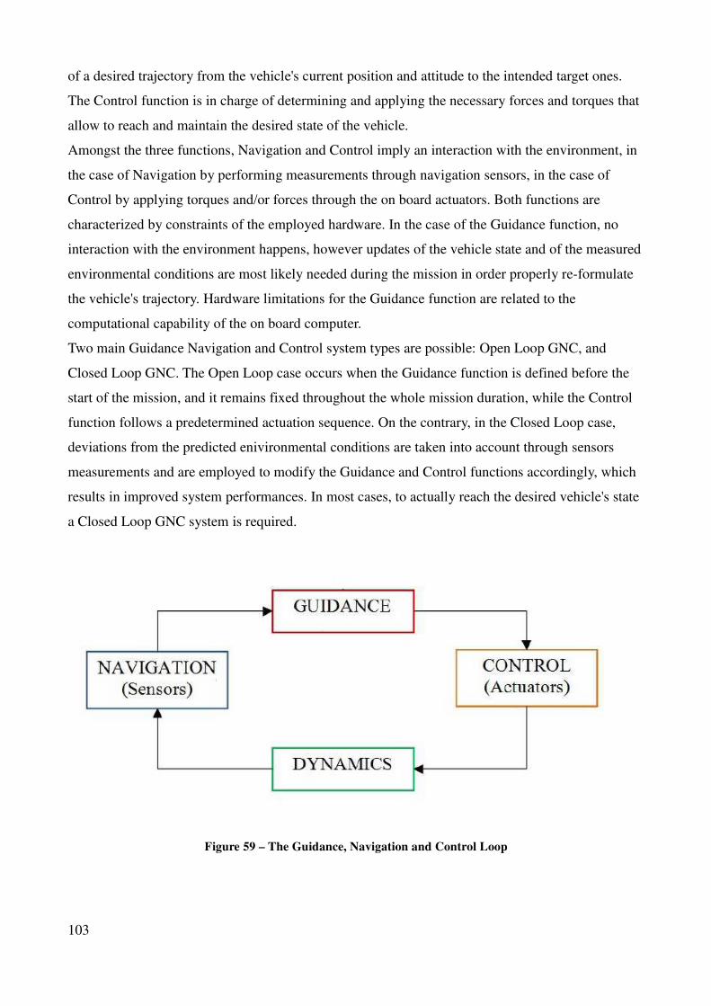
of a desired trajectory from the vehicle's current position and attitude to the intended target ones.
The Control function is in charge of determining and applying the necessary forces and torques that
allow to reach and maintain the desired state of the vehicle.
Amongst the three functions, Navigation and Control imply an interaction with the environment, in
the case of Navigation by performing measurements through navigation sensors, in the case of
Control by applying torques and/or forces through the on board actuators. Both functions are
characterized by constraints of the employed hardware. In the case of the Guidance function, no
interaction with the environment happens, however updates of the vehicle state and of the measured
environmental conditions are most likely needed during the mission in order properly re-formulate
the vehicle's trajectory. Hardware limitations for the Guidance function are related to the
computational capability of the on board computer.
Two main Guidance Navigation and Control system types are possible: Open Loop GNC, and
Closed Loop GNC. The Open Loop case occurs when the Guidance function is defined before the
start of the mission, and it remains fixed throughout the whole mission duration, while the Control
function follows a predetermined actuation sequence. On the contrary, in the Closed Loop case,
deviations from the predicted enivironmental conditions are taken into account through sensors
measurements and are employed to modify the Guidance and Control functions accordingly, which
results in improved system performances. In most cases, to actually reach the desired vehicle's state
a Closed Loop GNC system is required.
Figure 59 – The Guidance, Navigation and Control Loop
103
4.2.1 Guidance Function
In the problems of SFF, RVD, and proximity operations in general, the Guidance function is in
charge of generating reference trajectories for the whole state of the vehicle (position and attitude),
which are then used as input of the on board control system of the satellites. Satellite systems can be
operative in two main different types of space environments, with the formulation of the Guidance
function changing accordingly: Deep Space environments, and Planetary Orbital Environments.
Satellites that operate in Deep Space environments experience generally very low levels of orbital
disturbances. As a consequence, their relative dynamics can be reduced to the double integrator
form, and a formation can be maintained with very low fuel consumption, or even without fuel
consumption, if the formation geometry is properly planned.
On the other hand, satellites that carry out their tasks in Planetary Orbital Environments experience
orbital disturbances with effects that are most likely not negligible. A typical way in SFF to avoid
excessive fuel consumption in order to counterbalance the disturbances encountered in these
environments, is the employment of Passive Relative Orbits, i.e. periodic relative trajectories that
need limited position control actuations. With a certain Passive Relative Orbit chosen so that the
formation evaporation is prevented in nominal conditions, the orbit robustness to disturbances must
neverthless be evaluated, especially wrt gravity gradient, luni-solar perturbations, atmospheric drag,
electric charges acting on the satellites. In order to evaluate the robustness of these orbits, the HCW
equations have been modified with the inclusion of drag and J2 effects, however if the relative orbit
presents an eccentricity of 0.005, the error induced by neglecting the eccentricity becomes higher
that the error due to the neglect of J2. In order to incorporate both J2 and orbit eccentricity in the
equations, the relative motion has to expressed in the LVLH frame as function of the solutions of
the differential mean orbital elements.
4.2.2 Navigation Function
The Navigation function in the problems of SFF and proximity operations is in charge of providing
estimates of the absolute and relative states of the involved satellites.
According to [20], there can be three fundamental state estimation schemes in SFF: Centralized,
Decentralized and Hierarchic.
The case of the Centralized Architecture occurs when one satellite is designed as chief, while the
other satellites are followers, with each follower sending its measurements to the chief satellite
104
which processes them through a Kalman filter, and can then broadcast the processed estimations to
the followers.
In the Decentralized Architecture the state estimation effort is equally distributed over the satellites
of the formation, which implies a higher autonomy for each satellite with reduced inter-
communication links requirements. This architecture can be implemented in two different ways, in
one case every spacecraft performs an estimation of the state of the entire formation, while in the
other case each spacecraft estimates only its own state, which implies, wrt to the former solution,
higher synchronization requirements between the satellites when carrying out GNC tasks.
Last, the Hierarchic Architecture foresees state estimation at first for reduced groups of satellites in
the formation, with the results being subsequently gathered by the satellites that are designed with
higher hierarchy. In this way each cluster of satellites performs the ranging and orientation
estimations indipendently, with the expection of the chief of the cluster. Each chief of the cluster
gathers then with each other to form the higher level cluster.
For relative state estimation in SFF, a widely employed solution is the GPS, which through
differential navigation presents especiallu high accuracy in the position estimation, in the order of
few centimeters. For RVD and proximity operations, vision systems, LIDARs, laser rangers, and
infrared cameras are navigation systems that can be employed for relative state estimation in terms
of relative range and bearing angles.
4.2.3 Control Function
In the case of SFF, but also in the general case of robotic formations for ground or underwater
applications, the Control function has the goal of performing the coordination of multiple vehicles.
To achieve this objective, a minimum of one spacecraft has to track a certain relative state reference
wrt to another satellite, and the state of the latter has to be available to the former for the control law
elaboration. This definition of control law for this specific problem is referred to as Formation
Tracking Control Law. The general control architecture foresees three main levels. The first level is
the Spacecraft Local Control. At this level, the system S i is the ith spacecraft which presents
control input vector u i , and measurable state output y i . This level is therefore in charge of
computing the actuator vector and a performance indicator for each spacecraft, from the measured
spacecraft state output and the input reference state trajectory and commands. The second level is
given by the Formation Control. This block has the task of elaborating and sending the outputs of
105
the reference trajectory and commands to all the satellites, and the outputs of the performance
indicators of all satellites to the higher level, i.e. the Supervisor, which employs the measured
Formation Control output to determine the input to be sent back to the Formation Control.
Generally, the Formation Control is in charge of the absolute and relative attitude and position
control of each spacecraft of the formation.
The problem of defining a control law in SFF has been studied in the context of Formation Flying
Control (FCC) with the definition of five main architectures as proposed by [4].
The first one is the Leader/Follower Architecture (L/F). In the L/F architecture, one spacecraft is
designed as leader, with a certain absolute reference state to be tracked with its own individual
control, while the remaining satellites are designated as followers that track only the states of the
other nearest follower satellites. In terms of navigation, the L/F architecture presents a Hierarchical
organization with the formation reference state defined by the leader spacecraft.
Another FCC architecture is the Multiple-Input, Multiple-Output (MIMO) architecture: in this case,
every spacecraft of the formation is treated as the element of a MIMO plant, to which therefore
every method of modern control can be potentially be applied, e.g. Linear Quadratic Regulator
(LQR), Model Predictive Control (MPC), etc., resulting in an optimal, stable control.
A FCC architecture that is essentialy an hybrid between L/F and MIMO is the Cyclic architecture.
In the Cyclic architecture, the satellites of the formation have a more uniformly distributed control
with a non-hierarchical structure.
The other two main FCC architectures defined by [4] are the Virtual Structure architecture, and the
Behavioral architecture. The Virtual Structure architecture foresees the satellite formation as a
unique system, which has a certain reference state trajectory defined in accordance to the mission
target, with the actual motion and control for each satellite derived subsequently at an individual
level. This architecture is especially indicated for cases such as interferometric missions, in which
the spacecraft formation must be operative as the equivalent of a bigger satellite with a single
payload resulting from all the payloads of the formation, and therefore the formation has to move as
much as possible as a rigid body. In the Behavioral architecture, all satellites of the formation are
set to cooperate with each other in order to reach the intended formation configuration, by following
certain predetermined behavioral schemes that are implemented in for safety and stability reasons,
i.e. collision avoidance schemes, obstacle avoidance schemes, formation keeping schemes, etc.
In the case of the Control function for automated RVD and proximity maneuvers between two
satellites, the general architecture is considerably simplified. The position and attitude control is
carried out at a relative level in order to perform the maneuver, with the management of reference
trajectory and commands in charge of the on board computer of the spacecraft which actively
106
performs the maneuver. As in the case of SFF, certain behavioral schemes are implemented in order
to carry out this type of maneuvers, for instance collision avoidance schemes are relevant in this
case, since these maneuvers present an increased risk of impact between the satellites.
For the problems of SFF and proximity operations, four main types of controllers will be presented:
Proportional – Integral – Derivative (PID), Linear Quadratic Regulator (LQR), Model Predictive
Control (MPC).
The plant dynamics of the Linear Time Invariant (LTI) model employed in LQR and MPC control
syntheses can be written in state-space form as follows:
x (t )=A x (t)+B u( t ) (52)
y (t )=C x ( t ) (53)
with x (t ) the state vector, u (t ) the control input vector, y (t ) the output, A the state
matrix, B the control matrix, C the output matrix.
4.2.3.1 PID Control
The Proportional-Integral-Derivative (PID) controller is given by a control law consisting of three
components. The first component, the proportional component u p(t ) , is proportional to the
instantaneous control tracking error e (t) . The second component, the integral component
u i(t) , is proportional to the integral of e (t) . The third component, the derivative component
ud (t ) , is proportional to the time derivative of e (t) . The complete formulation of the control
law is given by:
uPID (t )=u p(t)+ui(t )+ud (t)=K p e( t )+K i∫0
t
e(τ )d τ+K d
d e(t )dt
(54)
with e (t)=r (t )− y (t) the control tracking error, y (t) the controlled variable, r (t) is the
reference signal, K p , K i , K d are respectively the proportional, integral and derivative
gains. The proportional term has the effect of compensating large control errors by increasing the
control action proportionally. The integral term introduces a pole at the origin of the complex plane,
resulting in the reduction to zero of the steady-state error with a step reference signal applied to the
107
system. The derivative action follows the predicted future values of the control errors and therefore
compensates for trends that are not predicted on part of the other two components. This basic
formulation is however modified in practical applications on the basis of three main aspects:
proportional and derivative kicks avoidance, saturation, low pass filtering of the derivative
components.
With regards to the first aspect, the proportional and derivative kicks appear with controllers that
have high gains which are set to produce fast disturbance rejection. This however results in
oscillatory responses to step set points. To compensate for proportional and derivative kicks, set
point weighting can be employed for both the derivative and proportional actions.
The problem of actuators saturation can be treated in PID controllers by employing a saturation
model in an anti-reset windup feedback scheme, so that the nonlinear behaviors introduced by
saturation are properly managed. Since in the occurence of saturation the system operates in open-
loop, feedback can be reintroduced by feeding back to the controller the difference between the
saturated and unsaturated control signal, so that the correct state of the controller is estimated.
With regards to the third aspect, a first-order low pass filter can be used in order to reduce the
effects of measurement noise in the control action.
With the inclusion of proportional and derivative kick avoidance, anti-reset windup feedback
scheme, and low pass filtering of the derivative component, the modified PID formulation can be
written as:
u (t )=K pβ r (t)− y (t)+1
T i
∫0
t
[e (τ)+ T i
K pT t
(u ' (t )− u (t))]d τ+T d [ d (γ r (t )− y f (t ))
dt ] (55)
T d
N
dy f (t)
t= y (t )− y f (t ) (56)
with u (t ) the computed control variable, u ' (t ) the process control input, T i=K p/K i ,
T d=K d /K p , β the proportional set-point weight, γ the derivative set-point weight, with
0≤ β≤ 1 , 0≤ γ≤ 1 in general.
108
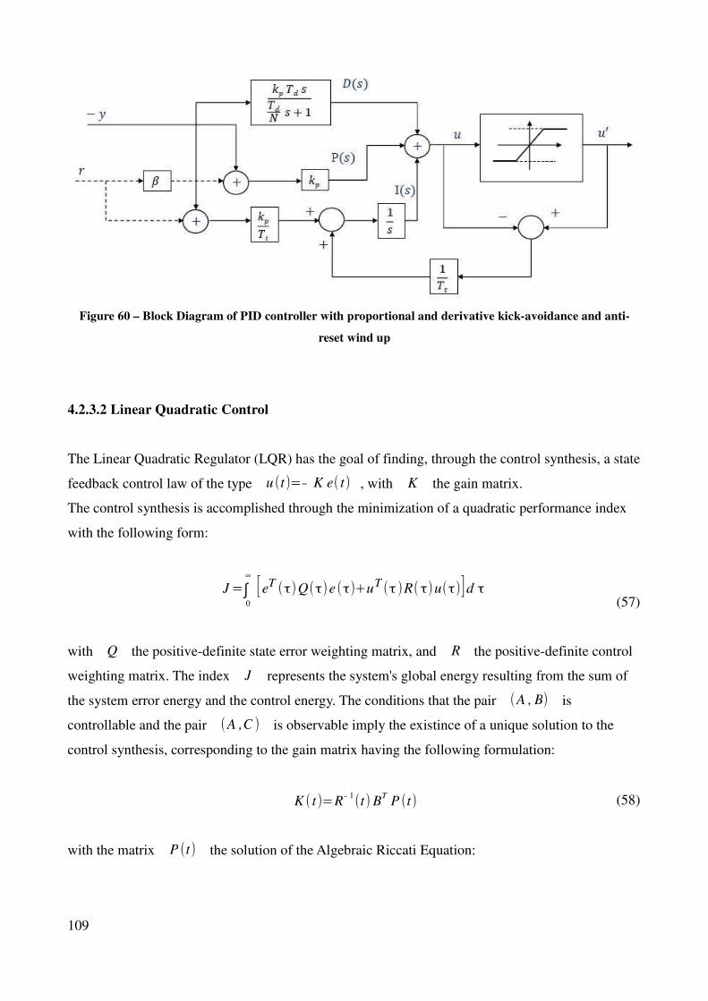
Figure 60 – Block Diagram of PID controller with proportional and derivative kick-avoidance and anti-
reset wind up
4.2.3.2 Linear Quadratic Control
The Linear Quadratic Regulator (LQR) has the goal of finding, through the control synthesis, a state
feedback control law of the type u (t )=− K e( t) , with K the gain matrix.
The control synthesis is accomplished through the minimization of a quadratic performance index
with the following form:
J=∫
0
∞
[eT (τ)Q(τ)e (τ)+uT (τ )R( τ)u(τ)]d τ (57)
with Q the positive-definite state error weighting matrix, and R the positive-definite control
weighting matrix. The index J represents the system's global energy resulting from the sum of
the system error energy and the control energy. The conditions that the pair (A , B) is
controllable and the pair (A ,C ) is observable imply the existince of a unique solution to the
control synthesis, corresponding to the gain matrix having the following formulation:
K ( t )=R− 1(t)BT
P (t) (58)
with the matrix P (t) the solution of the Algebraic Riccati Equation:
109
P (t)A+AT
P (t)− P( t)B R− 1( t )BT
P (t)+Q (t )=0 (59)
Matrices Q and R are arbitrary parameters, with values that must be chosen in accordance to
the characteristics of the system to be controlled, and to the desired performances in tracking the
reference trajectories, considering also the overall amount of control action spent during the
maneuver.
4.2.3.3 Model Predictive Control
Model Predictive Control (MPC) [22, 23, 24], also referred to as Receding Horizon Control (RHC),
consists in a modern optimal control technique that has been widely employed in industry in order
to solve multivariable constrained control problems [25, 26, 27]. In its basic formulation, MPC
foresees the employment of an explicit model of the plant that has to be controlled, and a sample of
the current state x t k in order to predict the future behavior of the output y (t ) over a finite
horizon of length p , as function of a control sequence. In this prediction of the future behavior
of the state, the control signal is assumed to be changing only in the interval [ t k , t k+m ] , while it
remains constant for the subsequent p− m control steps, with m≤ p , where p is the
length in time steps of the prediction horizon, and m is the length of the control horizon.
Through this prediction, the current control action to be applied is computed by solving an on-line
finite horizon open-loop optimal control problem, obtaining the optimal control sequence
U ' k ( x t k)=u ' t k
, u ' t k+1, .... , u ' tk+m that minimizes a certain system cost measure over the chosen
prediction horizon. With the optimal control sequence available, the subsequent step foreseen in the
MPC scheme, consists in applying only the first action of the sequence, and then solving back the
optimal control problem with a new state estimate at the subsequent time instant. In this way
feedback is introduced in the system, allowing compensation of possible modeling errors and/or
disturbances.
110
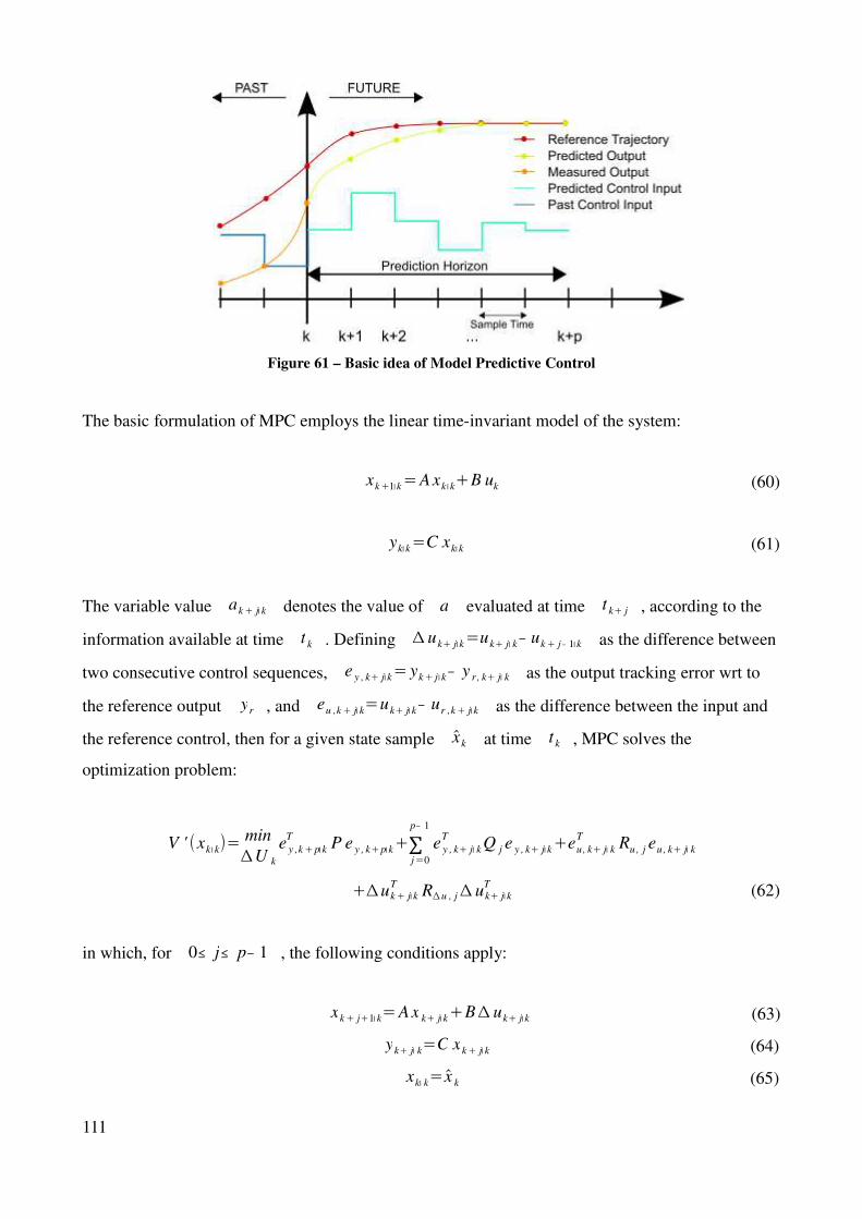
Figure 61 – Basic idea of Model Predictive Control
The basic formulation of MPC employs the linear time-invariant model of the system:
xk+1∣k=A xk ∣k+B uk (60)
yk∣k=C xk∣k (61)
The variable value ak+ j∣k denotes the value of a evaluated at time t k+ j , according to the
information available at time t k . Defining ∆ uk+ j∣k=uk+ j∣ k− uk+ j− 1∣k as the difference between
two consecutive control sequences, e y , k+ j∣k= yk+ j∣k− y r , k+ j∣ k as the output tracking error wrt to
the reference output yr , and eu ,k+ j∣k=uk+ j∣k− ur ,k+ j∣k as the difference between the input and
the reference control, then for a given state sample xk at time t k , MPC solves the
optimization problem:
V ' (xk ∣k)=min
∆U k
e y ,k+p∣k
TP e y , k+p∣k+∑
j=0
p− 1
e y , k+ j∣ k
TQ j e y , k+ j∣k+eu , k+ j∣ k
TRu , j eu , k+ j∣ k
+∆uk+ j∣k
TR∆u , j∆ uk+ j∣k
T (62)
in which, for 0≤ j≤ p− 1 , the following conditions apply:
xk+ j+1∣k=A x k+ j∣k+B∆ uk+ j∣k (63)
yk+ j∣ k=C xk+ j∣k (64)
xk∣ k= x k (65)
111
[E G ] [ yk+ j∣ k uk+ j∣k ]≤ L (66)
H ∆uk+ j∣k≤ M (67)
∆ uk+h=0,∀ h=m , .... , p− 1 (68)
with the optional terminal constraint E f yk+ p∣ k≤ L f .
The solution of the optimal control problem is given by the optimal control sequence:
∆U ' k=∆u ' k∣k ,∆u ' k+1∣k ,... ,∆u ' k+m− 1∣k (69)
the MPC control law can therefore be written as:
uk
MPC= uk− 1+∆u ' k∣k (70)
Equation [E G ] [ yk+ j∣ k uk+ j∣k ]T≤ L expresses a polyhedral constraint which includes different
types of constraints on the output and on the control input.
In the design of a MPC controller it has to be considered that a small prediction horizon p
,together with tight control constraints and high state error weight, implies a more aggressive
control with finer tracking performances but with higher control action expense. On the other hand,
a high control horizon m implies more optimality of the control, neverthless with higher
computational effort. Therefore the choice of the prediction and control horizons values should
result from a trade-off involving optimality, tracking performances, computational effort, and
memory allocation in the on-board processors.
4.2.3.3.1 Explicit Model Predictive Control
An explicit solution to LTI MPC problems that are constrained can be obtained by solving off-line a
multi-parametric Quadratic Program, as it has been shown by Bemporad et al. [28]. The explicit
solution is ideal for the case of plants which present processing systems with limited availability of
power and memory.
Considering the MPC problem:
112
min
U kx k+p∣k
TP xk+ p∣k+∑
i=0
p− 1
xk+i∣k
TQ x k+i∣k+uk+i
TR uk+i (71)
ymin≤ yk+i∣ k≤ ymax , i=1, ... , p (72)
umin≤ uk+i≤ umax , i=1, ... , m (73)
xk∣ k=x k= x( t k) (74)
xk+i+1∣ k=A xk+i∣k+B uk+i , i≥ 0 (75)
yk+i∣k=C xk+i∣ k (76)
uk+i=K xk+i∣k , m≤ i≤ p− 1 (77)
in which (A , B ) is a stabilizable pair. Assuming non active constraints when i≥ m and
i≥ p , then when the final cost matrix P and gain matrix K are computed from the
algebraic Riccati equation, the MPC problem solves exactly the constrained infinite horizon LQR
problem. Treating xk as a vector of parameters θk , Bemporad et al. showed that the MPC
problem can be rewritten as a multi-parametric Quadratic Program. For this multi-parametric
problem, the Karush-Kuhn-Tucker conditions are necessary and sufficient for optimality, which
guarantees the existence of a unique solution.
The resulting control law uMPC= f (θk ) is continuous and Piece Wise Affine:
f (θk)=Fiθk+g
i, if H
iθk≤ ki, i=1, ... , N MPC (78)
with N MPC standing for the number of neighbouring convex polytopes (or regions) in which the
theta-space is divided. With the control synthesis performed offline, the MPC computational effort
reduces eventually to a table lookup. In fact, when a given vector of parameters θk is known, the
control gains Fi and g
i are automatically determined by the polyhedral region Hiθk≤ k
i
which contains the parameters vector.
The explicit MPC formulation makes this type of control algorithm especially attractive for plants
that suffer from stringent on-line computational requirements. Deciding between an on-line MPC or
an explicit MPC controller should in any case derive from the comparison between the
computational effort required by the implicit solution and the memory allocation for the lookup
table of the explicit solution.
113
4.3 Planning of Control Maneuvers tests with the Matlab Software Simulator
This section presents some examples of control maneuvers planned with the Matlab Software
Simulator described in Section 2.5. The planned control maneuvers are of two main types, either 3
DOF maneuvers in position and Azimuth, in the case of the AM blocked through the additional
interface, or 5 DOF maneuvers in position and 3 DOF Attitude, with Yaw, Pitch, Roll provided by
the 3-axes joints structure of the AM.
4.3.1 Planning of 3 DOF Position and Azimuth Control Maneuvers
This section reports examples of control maneuvers performed with the Matlab Software Simulator
for the 3 DOF configuration of the complete Unit (See Figure (16) in Section (2.4.1.1) for the 3D
model representation). Two types of 2D position and Azimuth control maneuvers were planned
through the simulator: control maneuvers in standard formulation through PID, and in optimal
formulation through explicit MPC. The equations of motion integrated within the software
simulator in order to evaluate the Unit state, are :
m x=F x ,ctrl+F x , d (79)
m y=F y ,ctrl+F y ,d (80)
I z Θ=τΘ , ctrl+τΘ ,d (81)
with m the estimated mass of the complete Unit, F i , ctrl the position control force along the
ith axis, F i , d the disturbance force along the i
th axis, I z the estimated moment of inertia
about the Azimuth axis, τΘ , ctrl the control torque about the Azimuth axis, τΘ , d the disturbance
torque about the Azimuth axis. The three equations are integrated in the software simulator through
the Matlab ODE45 function.
4.3.1.1 Standard Control Maneuvers
The version of the Matlab Software Simulator allowing 2 translational and 1 rotational DOF
(Azimuth) was firstly employed for the planning of a position and attitude control maneuver with
PID position and attitude controllers. The PID controllers were implemented according to the
114
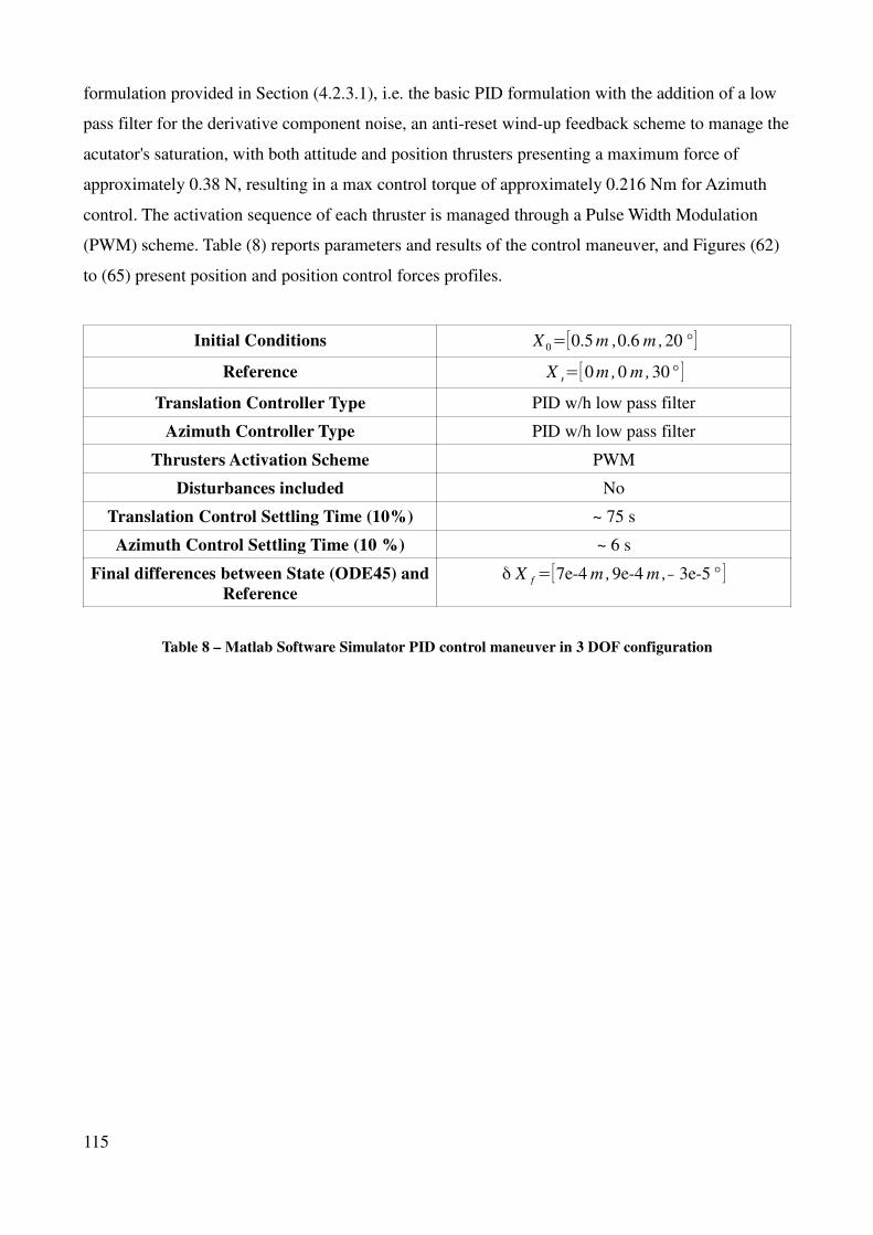
formulation provided in Section (4.2.3.1), i.e. the basic PID formulation with the addition of a low
pass filter for the derivative component noise, an anti-reset wind-up feedback scheme to manage the
acutator's saturation, with both attitude and position thrusters presenting a maximum force of
approximately 0.38 N, resulting in a max control torque of approximately 0.216 Nm for Azimuth
control. The activation sequence of each thruster is managed through a Pulse Width Modulation
(PWM) scheme. Table (8) reports parameters and results of the control maneuver, and Figures (62)
to (65) present position and position control forces profiles.
Initial Conditions X 0=[0.5 m ,0.6 m ,20 ° ]
Reference X r=[0 m , 0 m , 30° ]
Translation Controller Type PID w/h low pass filter
Azimuth Controller Type PID w/h low pass filter
Thrusters Activation Scheme PWM
Disturbances included No
Translation Control Settling Time (10%) ~ 75 s
Azimuth Control Settling Time (10 %) ~ 6 s
Final differences between State (ODE45) and
Reference
δ X f=[7e-4 m , 9e-4 m ,− 3e-5° ]
Table 8 – Matlab Software Simulator PID control maneuver in 3 DOF configuration
115
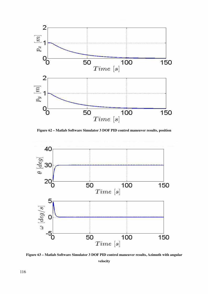
Figure 62 – Matlab Software Simulator 3 DOF PID control maneuver results, position
Figure 63 – Matlab Software Simulator 3 DOF PID control maneuver results, Azimuth with angular
velocity
116
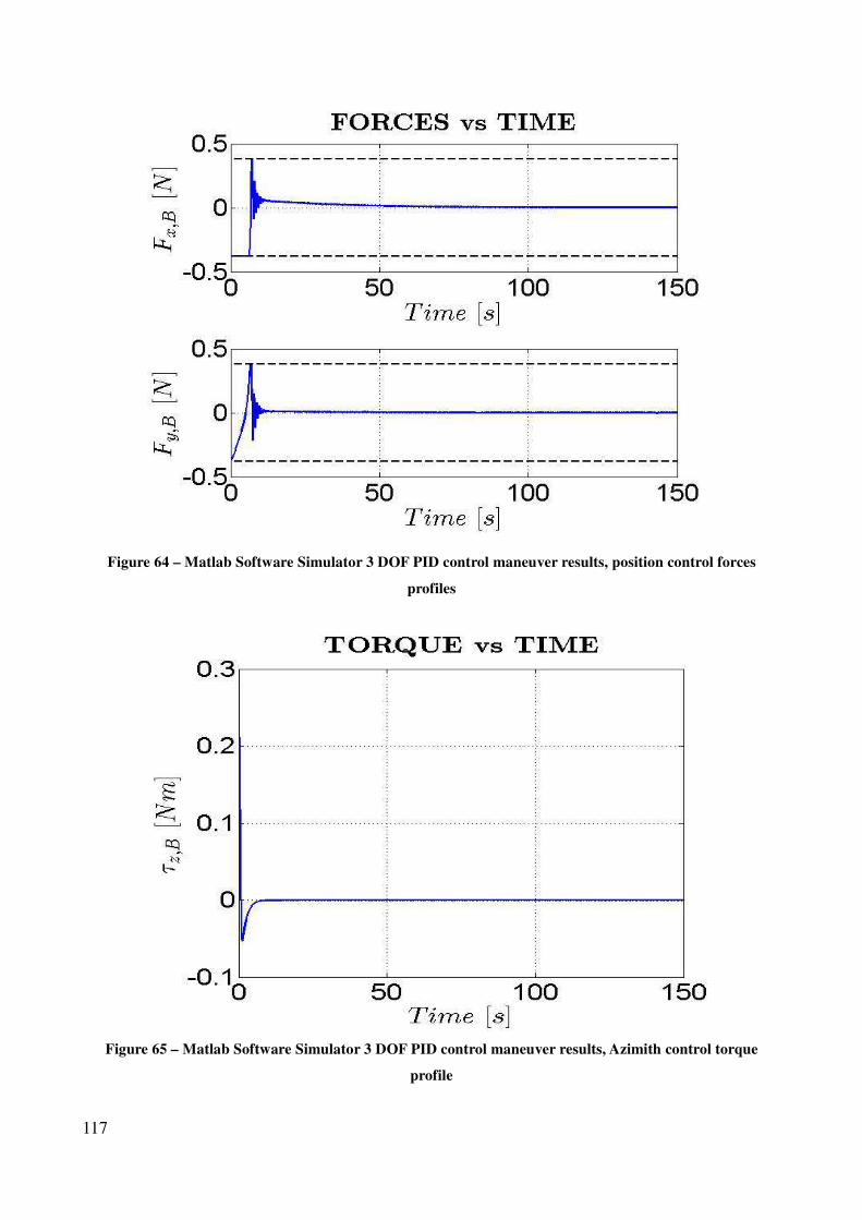
Figure 64 – Matlab Software Simulator 3 DOF PID control maneuver results, position control forces
profiles
Figure 65 – Matlab Software Simulator 3 DOF PID control maneuver results, Azimith control torque
profile
117
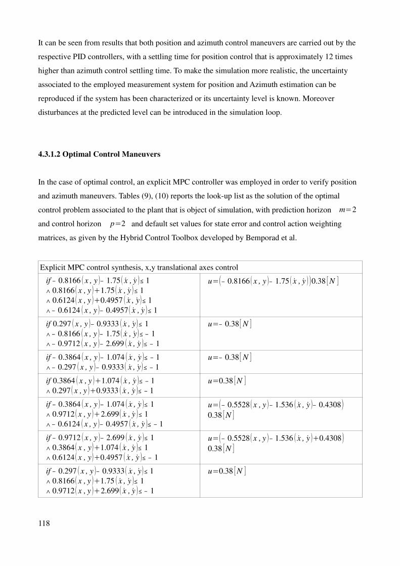
It can be seen from results that both position and azimuth control maneuvers are carried out by the
respective PID controllers, with a settling time for position control that is approximately 12 times
higher than azimuth control settling time. To make the simulation more realistic, the uncertainty
associated to the employed measurement system for position and Azimuth estimation can be
reproduced if the system has been characterized or its uncertainty level is known. Moreover
disturbances at the predicted level can be introduced in the simulation loop.
4.3.1.2 Optimal Control Maneuvers
In the case of optimal control, an explicit MPC controller was employed in order to verify position
and azimuth maneuvers. Tables (9), (10) reports the look-up list as the solution of the optimal
control problem associated to the plant that is object of simulation, with prediction horizon m=2
and control horizon p=2 and default set values for state error and control action weighting
matrices, as given by the Hybrid Control Toolbox developed by Bemporad et al.
Explicit MPC control synthesis, x,y translational axes control
if − 0.8166 (x , y )− 1.75( x , y )≤ 1
∧ 0.8166 ( x , y )+1.75( x , y )≤ 1
∧ 0.6124( x , y )+0.4957 ( x , y)≤ 1
∧− 0.6124 ( x , y )− 0.4957 ( x , y )≤ 1
u=(− 0.8166 ( x , y )− 1.75 ( x , y ))0.38 [N ]
if 0.297 ( x , y )− 0.9333 ( x , y)≤ 1
∧− 0.8166 (x , y )− 1.75( x , y)≤ − 1
∧− 0.9712 ( x , y )− 2.699 ( x , y )≤ − 1
u=− 0.38 [N ]
if − 0.3864 (x , y )− 1.074 ( x , y )≤ − 1
∧− 0.297 ( x , y )− 0.9333( x , y)≤ − 1
u=− 0.38 [N ]
if 0.3864 ( x , y )+1.074 ( x , y )≤ − 1
∧ 0.297(x , y )+0.9333 ( x , y )≤ − 1
u=0.38 [N ]
if − 0.3864 ( x , y )− 1.074 ( x , y )≤ 1
∧ 0.9712(x , y )+2.699( x , y )≤ 1
∧− 0.6124 ( x , y )− 0.4957 ( x , y )≤ − 1
u=(− 0.5528(x , y )− 1.536 ( x , y )− 0.4308)0.38 [N ]
if − 0.9712 ( x , y )− 2.699 ( x , y )≤ 1
∧ 0.3864( x , y)+1.074 ( x , y )≤ 1
∧ 0.6124( x , y)+0.4957 ( x , y )≤ − 1
u=(− 0.5528( x , y )− 1.536 ( x , y )+0.4308)0.38 [N ]
if − 0.297 (x , y )− 0.9333( x , y)≤ 1
∧ 0.8166( x , y )+1.75 ( x , y )≤ 1
∧ 0.9712( x , y )+2.699( x , y )≤ − 1
u=0.38 [N ]
118
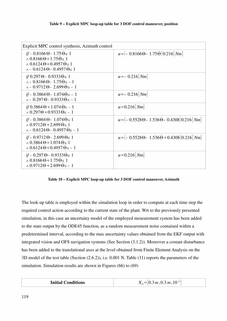
Table 9 – Explicit MPC loop-up table for 3 DOF control maneuver, position
Explicit MPC control synthesis, Azimuth control
if − 0.8166Θ− 1.75 Θ≤ 1
∧ 0.8166Θ+1.75Θ≤ 1
∧ 0.6124Θ+0.4957 Θ≤ 1∧− 0.6124Θ− 0.4957 Θ≤ 1
u=(− 0.8166Θ− 1.75Θ )0.216 [Nm ]
if 0.297Θ− 0.9333Θ≤ 1
∧− 0.8166Θ− 1.75Θ≤ − 1
∧− 0.9712Θ− 2.699 Θ≤ − 1
u=− 0.216 [Nm ]
if − 0.3864Θ− 1.074Θ≤ − 1
∧− 0.297Θ− 0.9333Θ≤ − 1
u=− 0.216 [Nm ]
if 0.3864Θ+1.074 Θ≤ − 1
∧ 0.297Θ+0.9333 Θ≤ − 1
u=0.216 [Nm]
if − 0.3864Θ− 1.074Θ≤ 1
∧ 0.9712Θ+2.699 Θ≤ 1
∧− 0.6124Θ− 0.4957 Θ≤ − 1
u=(− 0.5528Θ− 1.536Θ− 0.4308)0.216 [Nm]
if − 0.9712Θ− 2.699 Θ≤ 1
∧ 0.3864Θ+1.074 Θ≤ 1
∧ 0.6124Θ+0.4957 Θ≤ − 1
u=(− 0.5528Θ− 1.536Θ+0.4308)0.216 [Nm]
if − 0.297Θ− 0.9333Θ≤ 1
∧ 0.8166Θ+1.75Θ≤ 1∧ 0.9712Θ+2.699 Θ≤− 1
u=0.216 [Nm]
Table 10 – Explicit MPC loop-up table for 3 DOF control maneuver, Azimuth
The look-up table is employed within the simulation loop in order to compute at each time step the
required control action according to the current state of the plant. Wrt to the previously presented
simulation, in this case an uncertainy model of the employed measurement system has been added
to the state output by the ODE45 function, as a random measurement noise contained within a
predetermined interval, according to the max uncertainty values obtained from the EKF output with
integrated vision and OFS navigation systems (See Section (3.1.2)). Moreover a costant disturbance
has been added to the translational axes at the level obtained from Finite Element Analysis on the
3D model of the test table (Section (2.6.2)), i.e. 0.001 N. Table (11) reports the parameters of the
simulation. Simulation results are shown in Figures (66) to (69)
Initial Conditions X 0=[0.3 m ,0.3 m ,10 ° ]
119
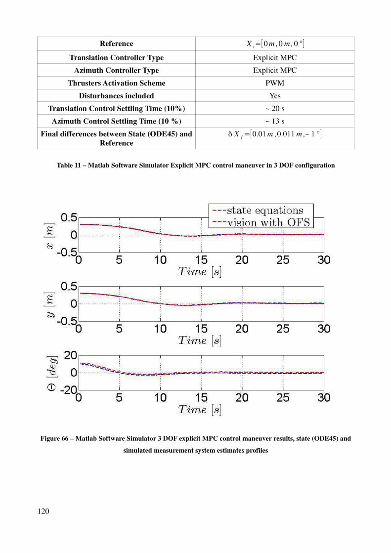
Reference X r=[0 m , 0 m , 0 ° ]
Translation Controller Type Explicit MPC
Azimuth Controller Type Explicit MPC
Thrusters Activation Scheme PWM
Disturbances included Yes
Translation Control Settling Time (10%) ~ 20 s
Azimuth Control Settling Time (10 %) ~ 13 s
Final differences between State (ODE45) and
Reference
δ X f=[0.01 m ,0.011 m ,− 1 ° ]
Table 11 – Matlab Software Simulator Explicit MPC control maneuver in 3 DOF configuration
Figure 66 – Matlab Software Simulator 3 DOF explicit MPC control maneuver results, state (ODE45) and
simulated measurement system estimates profiles
120
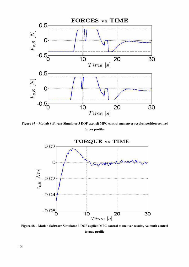
Figure 67 – Matlab Software Simulator 3 DOF explicit MPC control maneuver results, position control
forces profiles
Figure 68 – Matlab Software Simulator 3 DOF explicit MPC control maneuver results, Azimuth control
torque profile
121
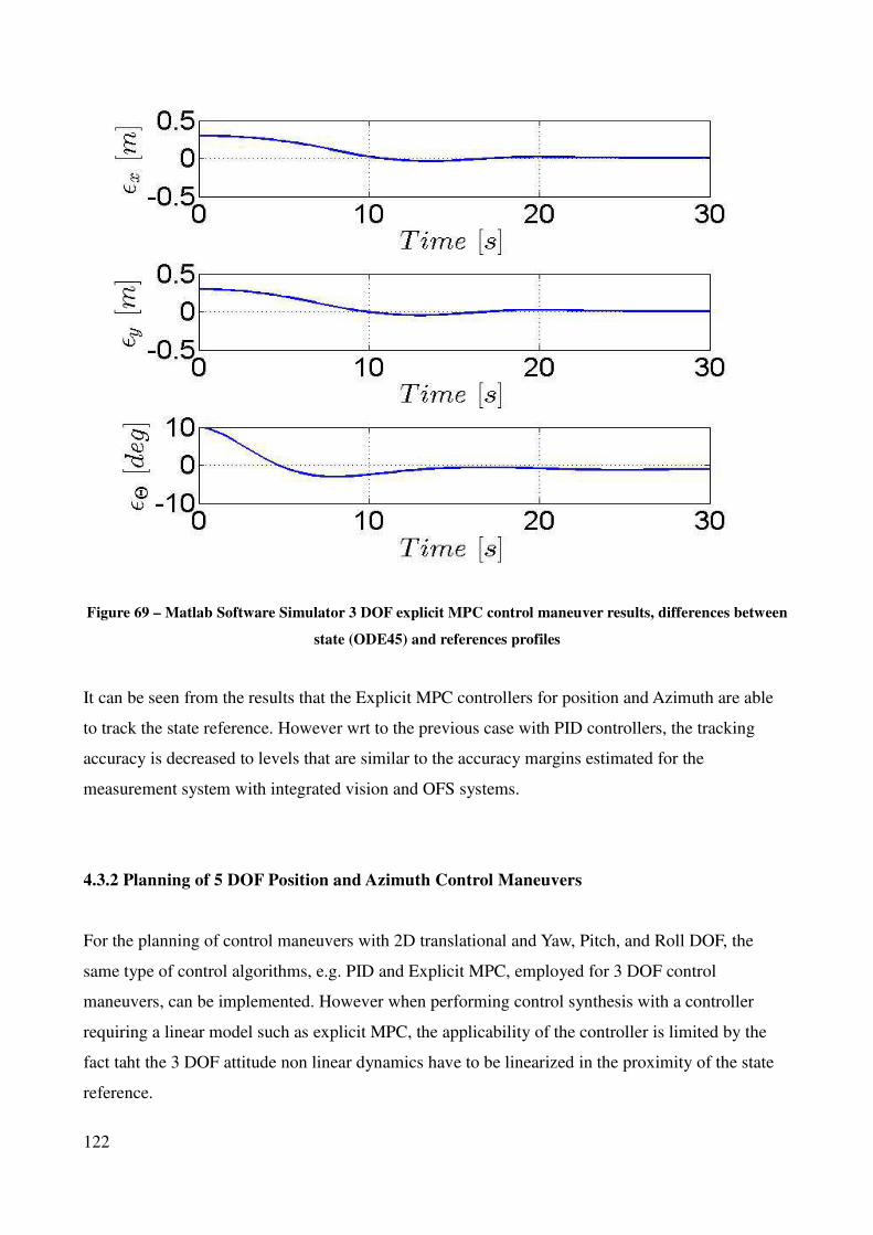
Figure 69 – Matlab Software Simulator 3 DOF explicit MPC control maneuver results, differences between
state (ODE45) and references profiles
It can be seen from the results that the Explicit MPC controllers for position and Azimuth are able
to track the state reference. However wrt to the previous case with PID controllers, the tracking
accuracy is decreased to levels that are similar to the accuracy margins estimated for the
measurement system with integrated vision and OFS systems.
4.3.2 Planning of 5 DOF Position and Azimuth Control Maneuvers
For the planning of control maneuvers with 2D translational and Yaw, Pitch, and Roll DOF, the
same type of control algorithms, e.g. PID and Explicit MPC, employed for 3 DOF control
maneuvers, can be implemented. However when performing control synthesis with a controller
requiring a linear model such as explicit MPC, the applicability of the controller is limited by the
fact taht the 3 DOF attitude non linear dynamics have to be linearized in the proximity of the state
reference.
122
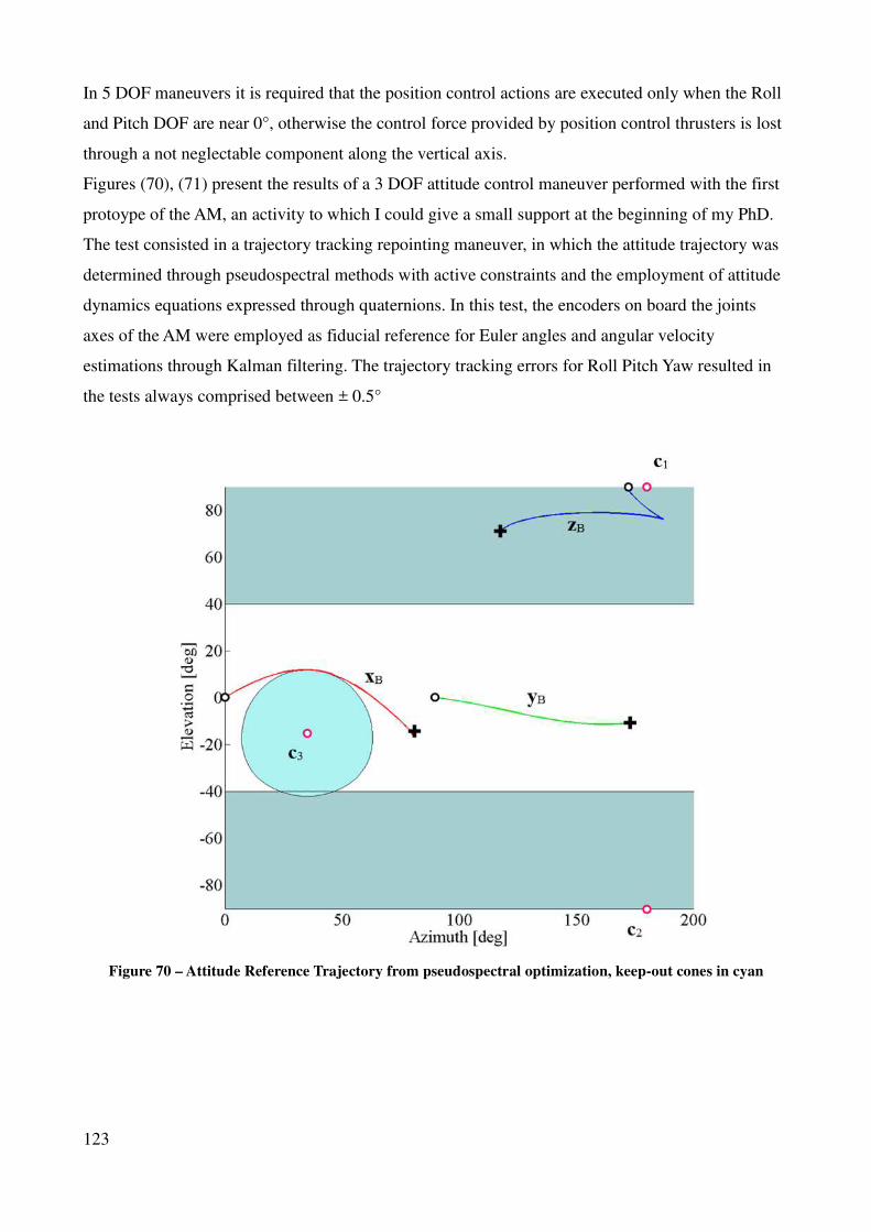
In 5 DOF maneuvers it is required that the position control actions are executed only when the Roll
and Pitch DOF are near 0°, otherwise the control force provided by position control thrusters is lost
through a not neglectable component along the vertical axis.
Figures (70), (71) present the results of a 3 DOF attitude control maneuver performed with the first
protoype of the AM, an activity to which I could give a small support at the beginning of my PhD.
The test consisted in a trajectory tracking repointing maneuver, in which the attitude trajectory was
determined through pseudospectral methods with active constraints and the employment of attitude
dynamics equations expressed through quaternions. In this test, the encoders on board the joints
axes of the AM were employed as fiducial reference for Euler angles and angular velocity
estimations through Kalman filtering. The trajectory tracking errors for Roll Pitch Yaw resulted in
the tests always comprised between ± 0.5°
Figure 70 – Attitude Reference Trajectory from pseudospectral optimization, keep-out cones in cyan
123
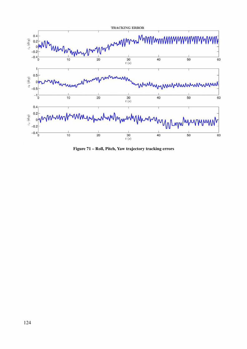
Figure 71 – Roll, Pitch, Yaw trajectory tracking errors
124

125
5 SCENARIO OF INSPECTION OF A NON COOPERATIVE TARGET SPACECRAFT IN
LEO THROUGH PASSIVE RELATIVE ORBIT ACQUISITION
5.1 Inspection Scenario Overview
This chapter presents the results from the investigation of a scenario related to the employment of
Passive Relative Orbits for the inspection of a non cooperative target spacecraft, as it is generally
the case for no more functioning satellites that have not been removed from their orbits.
In particular, the study is focused on assessing the performances in the employment of relative
circular orbits for inspection purposes, which implies the satisfaction of a predetermined set of
initial conditions that allow the inspection spacecraft to maintain a fixed distance wrt to the non
cooperative target satellite that must be inspected. One of the main goals of this analysis is the
subsequent reproduction of the satellite relative dynamics in scale through the SPARTANS
simulator.
In particular, a specific scenario has been considered of interest for this investigation, in terms of
evaluating the performances of LQR and MPC controllers in the acquisition and mainteinance of a
passive relative orbit of a generic spacecraft for the inspection of the Envisat satellite.
The Envisat (Environmental Satellite) satellite is an Earth-observation spacecraft which was
operated by ESA and built by Airbus Defence and Space. It was launched in 2002 with 10
instruments on board, designed to acquire important information regarding Earth meteorology,
climatology, environment, atmospheric chemestry, vegetation, hydrology, ocean and ice evolution.
After launch, the spacecraft was inserted in a sun-synchronous orbit at approximately 790 km of
altitude and an inclination of 98 °.
Compared to average satellites, the Envisat spacecraft presents very high dimensions, reaching 25 x
20 x 7 m in full deployment, with its solar panels occupying an area of 70 m2.
After 10 years of operations in orbit, in April 2012 the ESA ground segment of Envisat lost contact
with the satellite's communication system, and since then it was never more able to acquire it back.
The presence of such a large, unmonitored spacecraft in its nominal orbit constitutes a serious threat
in terms of collisions with other satellites, since at its nominal altitude and inclination there is a
probability that every year at least two satellites could pass below a distance of 200 m from it.
A collision between a spacecraft and Envisat can produce a very large debris cloud, which in turn
can trigger more and more collisions with other spacecraft with increasing rate and number of
newly produced debris, resulting in what could become a chain reaction with catastrophic
126
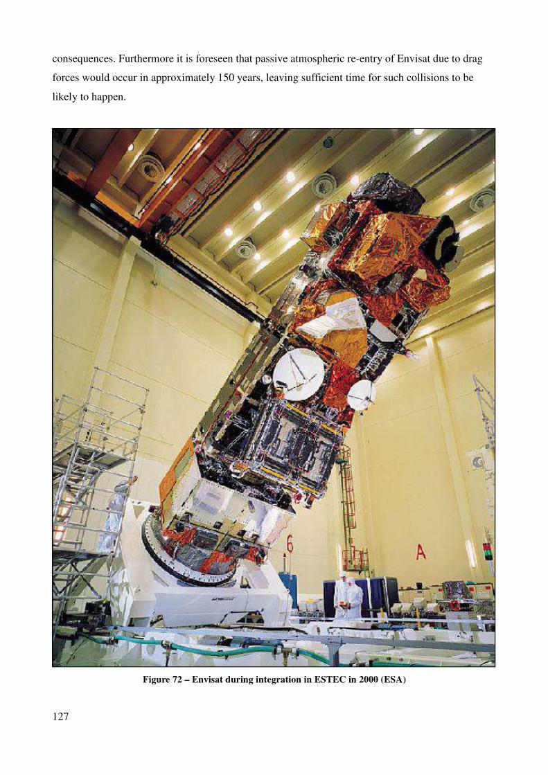
consequences. Furthermore it is foreseen that passive atmospheric re-entry of Envisat due to drag
forces would occur in approximately 150 years, leaving sufficient time for such collisions to be
likely to happen.
Figure 72 – Envisat during integration in ESTEC in 2000 (ESA)
127
It is therefore currently being envisioned a mission for the removal of Envisat from its nominal
orbit. The designed spacecraft would be approaching Envisat, monitoring it in a passive relative
orbit in order to assess its overall conditions, and it would subsequently perform a capture maneuver
at one of its appendices, in order to eventually drag it away from its orbit.
The analysis presented in this chapter is focused on the manuever for the acquisition and
mainteinance of a passive relative orbit for the inspection of the target satellite. The analysis has
been performed with the fundamental assumption that the relative state between the inspection and
the target satellite is available below a sufficiently low distance between the two, through a relative
measurement system that is assumed to be installed on board the inspection satellite. This
assumption is primarily based on results from recent numerical investigations related to this subject.
In particular, a recent study [35] considering a chaser and a target satellite, has shown that by
employing a vision system based on a sparse stereovision algorithm on board the chaser satellite,
the Body frame of the target spacecraft can be re-established by identifying its natural features, and
subsequently its translational and rotational states can be estimated through Kalman filtering of the
measurements. Numerical simulations for a target spacecraft in torque-free tumbling with maximum
initial angular velocity component of 3 °/s have shown that the proposed system reaches accuracies
in the order of 6 mm and 0.2 mm/s for the translational state estimation, and in the order of 0.1° and
0.03 °/s for the rotational state estimation, considering a target in the range of 10 m distance from
the chaser, and with general dimensions that are approximately one order of magnitude lower than
those of Envisat.
5.2 Definition of Relative Conditions and Disturbances
The fundamental condition in the proposed inspection scenario is related to the relative circular
orbit. Without external disturbances on the satellites' motion, the satisfaction of a certain set of
predetermined initial conditions produces a certain type of relative orbit that is maintained in time,
unless for errors in the initial conditions.
In the case of the relative circular orbit, the inspection satellite motion has to satisfy the following
relations between relative initial conditions, wrt to the target spacecraft:
δ y0=− 2 nδ x0 (82)
δ y0=2δ x0
n (83)
128
δ z0=±√3δ x0 (84)
δ z0=±√3δ x0 (85)
These conditons are obtained by imposing that δ x2+δ y
2+δ z2=r
2 in the solution of the HCW
equations, with r the radius of the formation. The first condition corresponds to the elimination
of the secular term, while the other three derive from the circularity of the relative orbit, with the
last two conditions to be taken with the same sign. The signs option implies that the relative orbit
plane is inclined of ± 60° wrt to the x-y plane of the LVLH frame.
Given these constraints on initial relative conditions, in the presence of external disturbances in the
satellites motions, and in presence of errors in the constraints satisfaction at the moment of
acquisition of the relative circular orbit, there is a more or less rapid and dramatic modification in
the initial geometry of the relative orbit.
With the inspection spacecraft motion initially taking place in a generic relative orbit wrt to the
target satellite, the satisfaction of the constraints on initial conditions of the inspection relative orbit
depends heavily on the precision with which the orbit acquisition maneuver is performed, and
therefore on the employed controller. With regards to disturbances, they are treated by periodically
activating the orbital control in order to re-establish the initial, desired value of the distance between
the inspection and the target spacecraft, when the distance exceeds a certain threshold value.
In this investigation the only disturbances that are considered in software simulations are those
related to differential drag forces, and those deriving from the J2 Earth gravitational potential term.
The disturbances caused by the J3 Earth gravitational potential term have been neglected by virtue
of the small eccentricity of the target and inspector orbits.
5.2.1 Relative Acceleration Disturbance due to J2
The relative effects caused by the J2 Earth gravity potential term are modeled through the gradient
of the J2 potential field [36]. The linear relative J2 disturbance in the LVLH frame is given by
multiplication of the relative position vector expressed in the LVLH frame by the J2 gradient
matrix:
δ a J2=∇ J 2δ x (86)
129
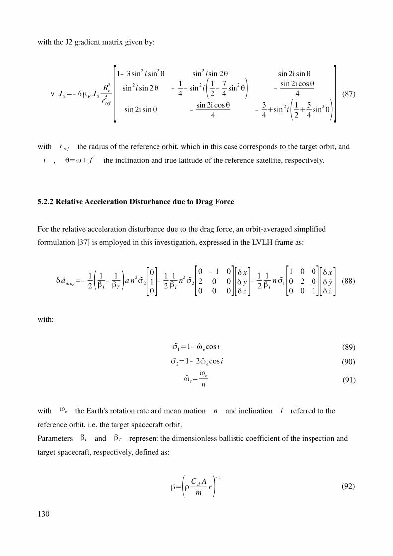
with the J2 gradient matrix given by:
∇ J 2=− 6µE J 2
Re
2
rref
5 [1− 3sin
2i sin
2θ sin2isin 2θ sin 2i sinθ
sin2i sin 2θ −
1
4− sin
2i(1
2−
7
4sin
2θ) −sin 2i cosθ
4
sin 2i sinθ −sin 2i cosθ
4−
3
4+sin
2i(1
2+
5
4sin
2θ)] (87)
with r ref the radius of the reference orbit, which in this case corresponds to the target orbit, and
i , θ=ω+ f the inclination and true latitude of the reference satellite, respectively.
5.2.2 Relative Acceleration Disturbance due to Drag Force
For the relative acceleration disturbance due to the drag force, an orbit-averaged simplified
formulation [37] is employed in this investigation, expressed in the LVLH frame as:
δ adrag=−1
2( 1β I
−1βT)a n
2σ2[010]− 1
2
1β I
n2 σ2[0 − 1 0
2 0 0
0 0 0][δ x
δ yδ z ]− 1
2
1β I
n σ1[1 0 0
0 2 0
0 0 1][δ x
δ yδ z ] (88)
with:
σ1=1− ωe cos i (89)
σ2=1− 2ωe cos i (90)
ωe=ωe
n (91)
with ωe the Earth's rotation rate and mean motion n and inclination i referred to the
reference orbit, i.e. the target spacecraft orbit.
Parameters βI and βT represent the dimensionless ballistic coefficient of the inspection and
target spacecraft, respectively, defined as:
β=(ρ C d A
mr)
− 1
(92)
130
with ρ the local atmospheric density, C d the drag coefficient of the spacecraft, A the
cross sectional area of the spacecraft, m the mass of the spacecraft, r the radius of the
spacecraft orbit.
5.3 Overview of the Formation Flight Software Simulator in Matlab
In order to test the aforementioned control techniques in the context of the proposed scenario, a
software simulator in Matlab has been updated and employed. The simulator in its fundamental
structure had already been developed in the context of the SPARTANS research team, with the goal
of the testing and validating GNC strategies for general formation flying applications. The simulator
presents a modular structure, allowing different elements of the software to be designed separately
and to subsequently evaluate its efficiency and robustness.
The main modules of the software simulator consists in the Dynamic Propagator module, the
Sensors module, the Navigation module, the Guidance module, the Control module, the Actuators
module, the Environment module.
The Dynamic Propagator module is in charge of estimating the dynamic evolution of the plant, by
integrating the system of differential equations that models the system dynamic behaviour,
expressed in the form:
X ( t )=F ( X (t ) , t ,U comm( t ) , U d (t)) (93)
with X ( t) the dynamic state of the plant, comprising environment, sensors, actuators, attitude
and orbital states, both absolute and relative, for each satellite in the formation, U comm(t ) the
control vector formed by position and attitude accelerations to be imposed to the system through the
actuators, U d (t) the disturbance acceleration vector. The input of the Dynamic Propagator is
given by the plant state X ( t k) at time step t k , the computed control accelerations
U comm(t) , the disturbance accelerations U d (t) . The output of the Dynamic Propagator is
given by the plant state X ( t k+1) at time step t k+1=t k+∆T S , with ∆T S the simulation
time step. The Dynamic Propagator module performs motion propagation through fixed time step
integration of the system of six differential equations that describe the satellites motion, expressed
131
in the cartesian Earth Centered Inertial frame of reference, with time as independent variable.
The Sensors module is intended, through a proper model of the employed sensors, to reproduce the
measurements of the system dynamic state as they are most likely to result. The measurement
model can comprise a bias and a white noise components to be added to the plant state.
The Navigation module is in charge of performing the estimation of the current state of the system
by employing the measurements that are output by the Sensors module, and a set of equations
describing the dynamic behaviour of the system and the behaviour of the sensors. Current state
estimation can be performed by the module through different estimation techniques, e.g. Kalman
filtering, Bayessian estimation.
The Guidance module is in charge of computing the desired trajectories as reference for the state for
each spacecraft of the formation, considering disturbances acting on the system, the current
estimated state of the system, the actuators characteristics.
The Control module has the function of computing the control actions U calc(t ) that have to be
performed by the actuators with the purpose of making the current estimated system state X ( t )
reach the reference state X ( t ) . The input of the Control module is given by estimated system
state X ( t ) at time t k , the reference trajectory X ( t k) at time t k , the disturbances acting
on the system, and the actuators constraints.
The Actuators module is in charge of determining the actual control action that is going to be
executed within the simulation. This module takes as input the control action vector
U calc(t k ) output by the Control module at time step t k , and the plant dynamic state
X ( t k) at time t k , in order to determine through the model equations of the actuators
describing their behaviour, the control action vector U comm(t k ) to be executed by the actuators at
time step t k .
The Environment module is in charge of computing the perturbative accelerations, acting on the
satellites of the formation, caused by interaction with the environment.
The formation flight simulator has been developed in Matlab through Object Oriented Programming
(OOP). Amongst the most important characteristics of OOP there is the concept of data
encapsulation, which implies the presence of a close link between data items and methods. Objects
of a given type are generally instances of a class, which is defined in order to provide internal
definition as well as public interface of its objects. The OOP presents the following advantages wrt
to procedural programming: reduced program complexity, modularity, increased ease in performing
program modifications, extensibility, and re-usability of objects for different programs.
132
The formation flight simulator in Matlab is composed of three main sections. The first section has a
pre-processing function, defining and initializing all objects, structures and variables of the
scenario. The second section consists of the main loop with a sequence of update of all modules at
each simulation time step. The third section consists of the post-processing with final computations,
and the saving and visualization of results. For each class, the interface functions can be divided in
setup functions, used to initialize the objects during pre-processing, update and data printing
functions used in the main loop to update the objects and visualize data in the command window at
the current simulation time step, and post-processing functions, which are used to save results and
create plots. A Set-Up m-file is employed in order to define the parameters of the scenario, i.e.
absolute and relative dynamic states of the satellites, type of sensors, actuators, GNC strategy, etc.
5.4 Matlab Simulations Results
This section reports the results from the simulations performed for the proposed inspection scenario.
Three main types of simulations have been performed. The first type consisted in the inspection
scenario of the Envisat satellite with the inspection passive relative orbit acquired through a pre-
computed 2 impulses maneuver, and orbit correction maneuvers performed with LQR and MPC
controllers. The second type of simulations consisted in both the inspection orbit acquisition and
correction maneuvers performed with the LQR controller, and the third type of simulations
consisted in both the inspection orbit acquisition and correction maneuvers performed with the
MPC controller.
The three types of simulations were performed with the same set of initial relative conditions
between the inspection and the target satellite, and the same set of final conditions at the acquisition
of the relative orbit for the inspection. In all three cases the final inspection orbit is circular with a
radius of approximately 40 m. For the estimation of the relative disturbance due to drag, in the case
of Envisat its nominal data have been considered in order to determine its dimensionless ballistic
coefficient, while in the case of the inspection satellite a hypotetic value has been taken,
representative for a spacecraft with average size and mass.
In both types of simulations, the initial relative orbit consists in an ellipse with semi-major axis of
approximately 120 m and semi-minor axis of approximately 60 m, i.e. a flyaround orbit acquired
through a previous initial relative approach. From the flyaround orbit, the inspection satellite is then
directly inserted in the inspection orbit (Figure (73)).
133
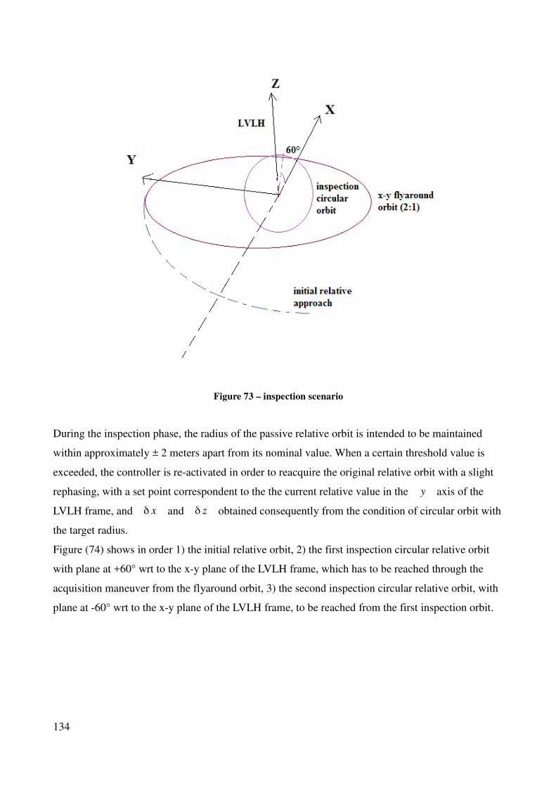
Figure 73 – inspection scenario
During the inspection phase, the radius of the passive relative orbit is intended to be maintained
within approximately ± 2 meters apart from its nominal value. When a certain threshold value is
exceeded, the controller is re-activated in order to reacquire the original relative orbit with a slight
rephasing, with a set point correspondent to the the current relative value in the y axis of the
LVLH frame, and δ x and δ z obtained consequently from the condition of circular orbit with
the target radius.
Figure (74) shows in order 1) the initial relative orbit, 2) the first inspection circular relative orbit
with plane at +60° wrt to the x-y plane of the LVLH frame, which has to be reached through the
acquisition maneuver from the flyaround orbit, 3) the second inspection circular relative orbit, with
plane at -60° wrt to the x-y plane of the LVLH frame, to be reached from the first inspection orbit.
134
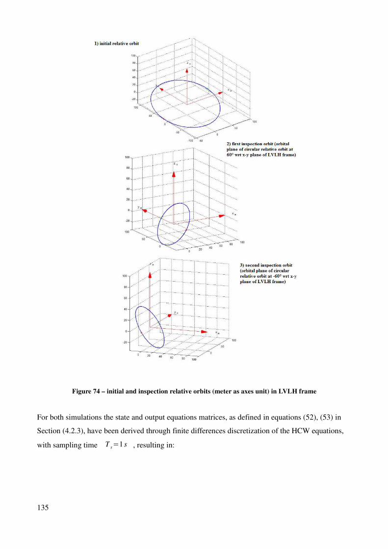
Figure 74 – initial and inspection relative orbits (meter as axes unit) in LVLH frame
For both simulations the state and output equations matrices, as defined in equations (52), (53) in
Section (4.2.3), have been derived through finite differences discretization of the HCW equations,
with sampling time T s=1 s , resulting in:
135
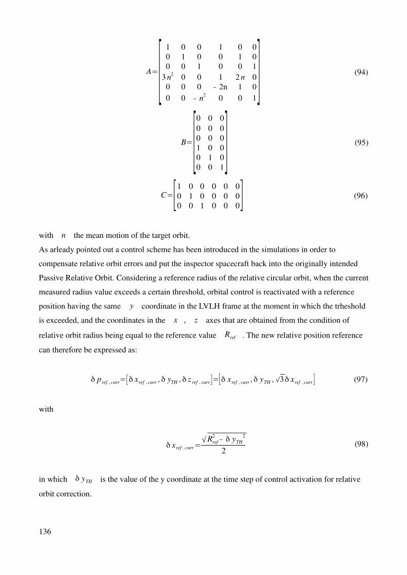
A=[1 0 0 1 0 0
0 1 0 0 1 0
0 0 1 0 0 1
3 n2
0 0 1 2 n 0
0 0 0 − 2n 1 0
0 0 − n2
0 0 1] (94)
B=[0 0 0
0 0 0
0 0 0
1 0 0
0 1 0
0 0 1] (95)
C=[1 0 0 0 0 0
0 1 0 0 0 0
0 0 1 0 0 0] (96)
with n the mean motion of the target orbit.
As arleady pointed out a control scheme has been introduced in the simulations in order to
compensate relative orbit errors and put the inspector spacecraft back into the originally intended
Passive Relative Orbit. Considering a reference radius of the relative circular orbit, when the current
measured radius value exceeds a certain threshold, orbital control is reactivated with a reference
position having the same y coordinate in the LVLH frame at the moment in which the trheshold
is exceeded, and the coordinates in the x , z axes that are obtained from the condition of
relative orbit radius being equal to the reference value Rref . The new relative position reference
can therefore be expressed as:
δ pref , curr=[δ xref ,curr ,δ yTH ,δ z ref , curr ]=[δ xref , curr ,δ yTH ,√3δ xref ,curr ] (97)
with
δ xref ,curr=√Rref
2− δ yTH
2
2 (98)
in which δ yTH is the value of the y coordinate at the time step of control activation for relative
orbit correction.
136
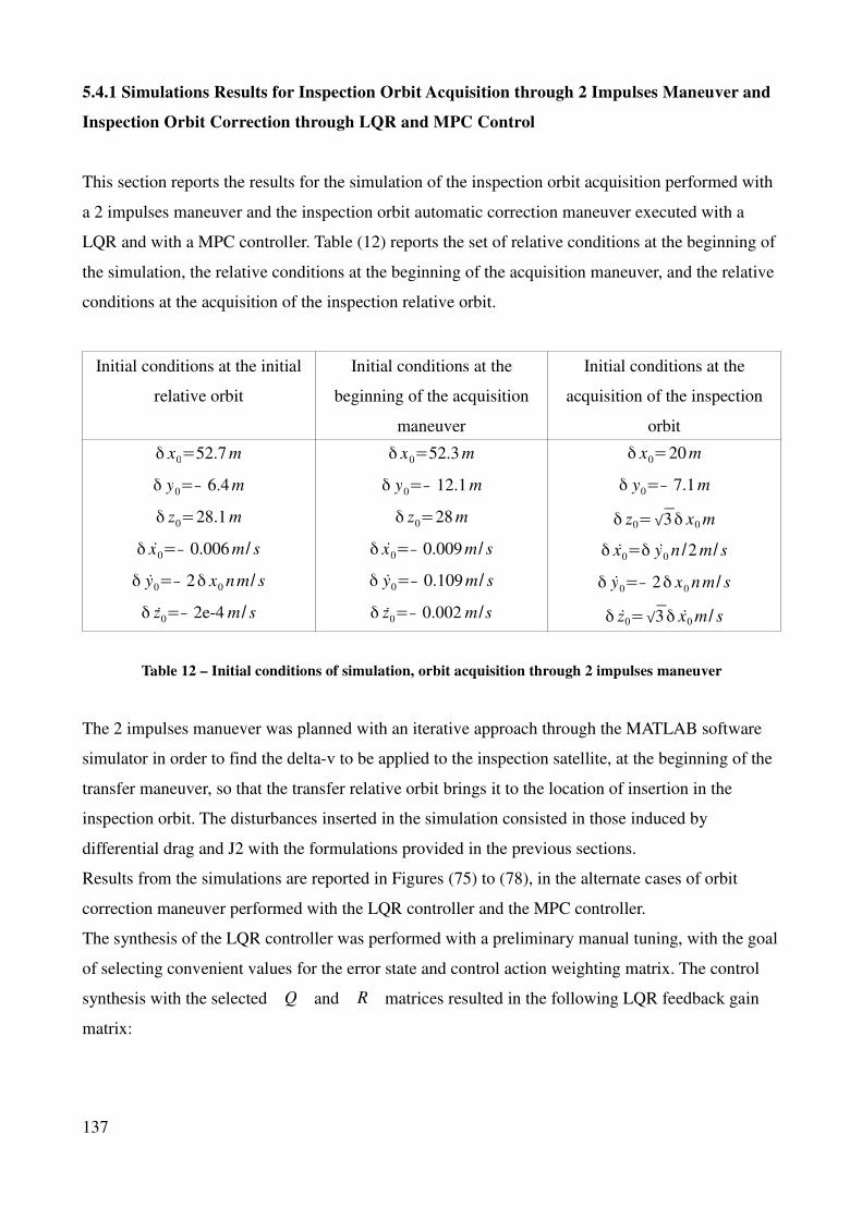
5.4.1 Simulations Results for Inspection Orbit Acquisition through 2 Impulses Maneuver and
Inspection Orbit Correction through LQR and MPC Control
This section reports the results for the simulation of the inspection orbit acquisition performed with
a 2 impulses maneuver and the inspection orbit automatic correction maneuver executed with a
LQR and with a MPC controller. Table (12) reports the set of relative conditions at the beginning of
the simulation, the relative conditions at the beginning of the acquisition maneuver, and the relative
conditions at the acquisition of the inspection relative orbit.
Initial conditions at the initial
relative orbit
Initial conditions at the
beginning of the acquisition
maneuver
Initial conditions at the
acquisition of the inspection
orbit
δ x0=52.7 m
δ y0=− 6.4m
δ z0=28.1 m
δ x0=− 0.006 m / s
δ y0=− 2δ x0 n m / s
δ z0=− 2e-4 m / s
δ x0=52.3 m
δ y0=− 12.1 m
δ z0=28 m
δ x0=− 0.009m / s
δ y0=− 0.109m / s
δ z0=− 0.002 m /s
δ x0=20 m
δ y0=− 7.1m
δ z0=√3δ x0 m
δ x0=δ y0 n /2 m / s
δ y0=− 2δ x0 n m / s
δ z0=√3δ x0 m / s
Table 12 – Initial conditions of simulation, orbit acquisition through 2 impulses maneuver
The 2 impulses manuever was planned with an iterative approach through the MATLAB software
simulator in order to find the delta-v to be applied to the inspection satellite, at the beginning of the
transfer maneuver, so that the transfer relative orbit brings it to the location of insertion in the
inspection orbit. The disturbances inserted in the simulation consisted in those induced by
differential drag and J2 with the formulations provided in the previous sections.
Results from the simulations are reported in Figures (75) to (78), in the alternate cases of orbit
correction maneuver performed with the LQR controller and the MPC controller.
The synthesis of the LQR controller was performed with a preliminary manual tuning, with the goal
of selecting convenient values for the error state and control action weighting matrix. The control
synthesis with the selected Q and R matrices resulted in the following LQR feedback gain
matrix:
137
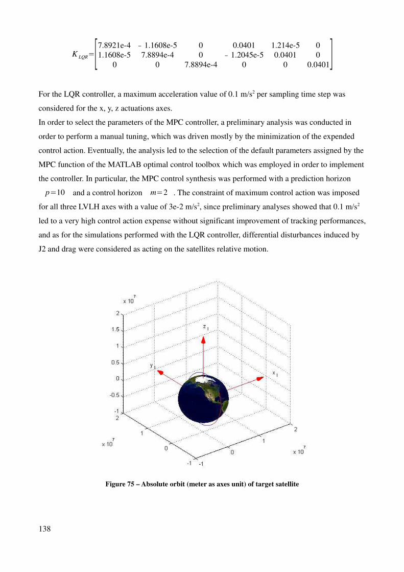
K LQR=[7.8921e-4 − 1.1608e-5 0 0.0401 1.214e-5 0
1.1608e-5 7.8894e-4 0 − 1.2045e-5 0.0401 0
0 0 7.8894e-4 0 0 0.0401]For the LQR controller, a maximum acceleration value of 0.1 m/s2 per sampling time step was
considered for the x, y, z actuations axes.
In order to select the parameters of the MPC controller, a preliminary analysis was conducted in
order to perform a manual tuning, which was driven mostly by the minimization of the expended
control action. Eventually, the analysis led to the selection of the default parameters assigned by the
MPC function of the MATLAB optimal control toolbox which was employed in order to implement
the controller. In particular, the MPC control synthesis was performed with a prediction horizon
p=10 and a control horizon m=2 . The constraint of maximum control action was imposed
for all three LVLH axes with a value of 3e-2 m/s2, since preliminary analyses showed that 0.1 m/s2
led to a very high control action expense without significant improvement of tracking performances,
and as for the simulations performed with the LQR controller, differential disturbances induced by
J2 and drag were considered as acting on the satellites relative motion.
Figure 75 – Absolute orbit (meter as axes unit) of target satellite
138
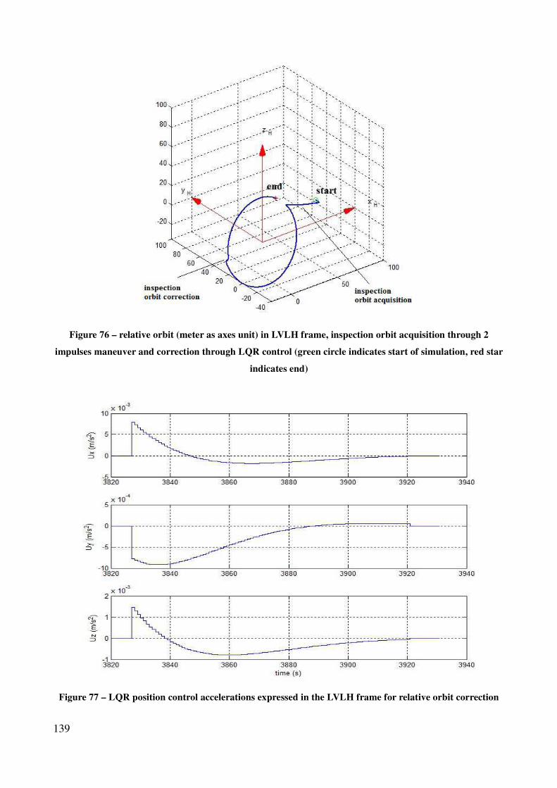
Figure 76 – relative orbit (meter as axes unit) in LVLH frame, inspection orbit acquisition through 2
impulses maneuver and correction through LQR control (green circle indicates start of simulation, red star
indicates end)
Figure 77 – LQR position control accelerations expressed in the LVLH frame for relative orbit correction
139
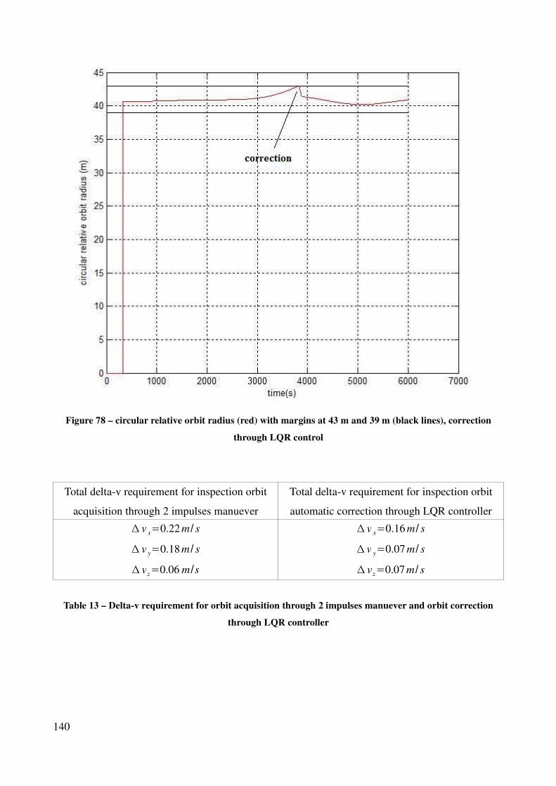
Figure 78 – circular relative orbit radius (red) with margins at 43 m and 39 m (black lines), correction
through LQR control
Total delta-v requirement for inspection orbit
acquisition through 2 impulses manuever
Total delta-v requirement for inspection orbit
automatic correction through LQR controller
∆ v x=0.22 m / s
∆ v y=0.18m / s
∆ vz=0.06 m /s
∆ v x=0.16 m / s
∆ v y=0.07 m / s
∆ vz=0.07 m / s
Table 13 – Delta-v requirement for orbit acquisition through 2 impulses manuever and orbit correction
through LQR controller
140
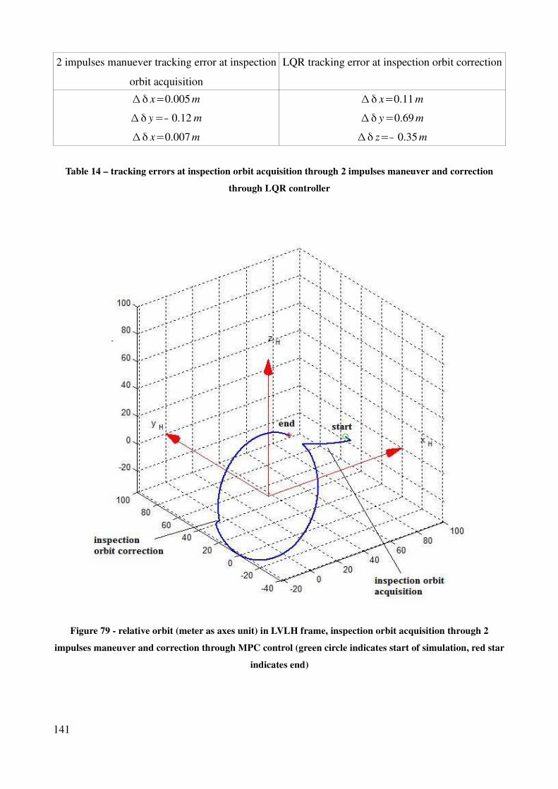
2 impulses manuever tracking error at inspection
orbit acquisition
LQR tracking error at inspection orbit correction
∆ δ x=0.005 m
∆ δ y=− 0.12 m
∆δ x=0.007 m
∆ δ x=0.11 m
∆ δ y=0.69m
∆δ z=− 0.35 m
Table 14 – tracking errors at inspection orbit acquisition through 2 impulses maneuver and correction
through LQR controller
Figure 79 - relative orbit (meter as axes unit) in LVLH frame, inspection orbit acquisition through 2
impulses maneuver and correction through MPC control (green circle indicates start of simulation, red star
indicates end)
141
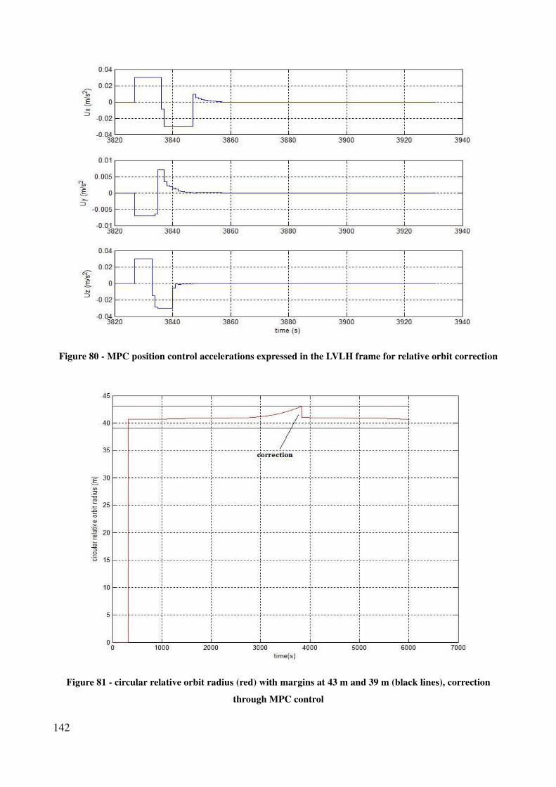
Figure 80 - MPC position control accelerations expressed in the LVLH frame for relative orbit correction
Figure 81 - circular relative orbit radius (red) with margins at 43 m and 39 m (black lines), correction
through MPC control
142
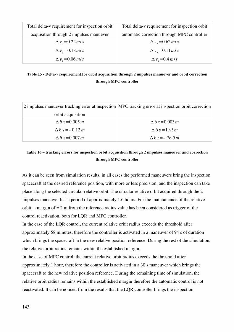
Total delta-v requirement for inspection orbit
acquisition through 2 impulses manuever
Total delta-v requirement for inspection orbit
automatic correction through MPC controller
∆ v x=0.22 m / s
∆ v y=0.18 m / s
∆ vz=0.06 m /s
∆ v x=0.62 m / s
∆ v y=0.11m / s
∆ vz=0.4 m /s
Table 15 - Delta-v requirement for orbit acquisition through 2 impulses manuever and orbit correction
through MPC controller
2 impulses manuever tracking error at inspection
orbit acquisition
MPC tracking error at inspection orbit correction
∆ δ x=0.005 m
∆δ y=− 0.12 m
∆δ x=0.007 m
∆ δ x=0.003 m
∆ δ y=1e-5m
∆ δ z=− 7e-5m
Table 16 – tracking errors for inspection orbit acquisition through 2 impulses maneuver and correction
through MPC controller
As it can be seen from simulation results, in all cases the performed maneuvers bring the inspection
spacecraft at the desired reference position, with more or less precision, and the inspection can take
place along the selected circular relative orbit. The circular relative orbit acquired through the 2
impulses maneuver has a period of approximately 1.6 hours. For the maintainance of the relative
orbit, a margin of ± 2 m from the reference radius value has been considered as trigger of the
control reactivation, both for LQR and MPC controller.
In the case of the LQR control, the current relative orbit radius exceeds the threshold after
approximately 58 minutes, therefore the controller is activated in a maneuver of 94 s of duration
which brings the spacecraft in the new relative position reference. During the rest of the simulation,
the relative orbit radius remains within the established margin.
In the case of MPC control, the current relative orbit radius exceeds the threshold after
approximately 1 hour, therefore the controller is activated in a 30 s maneuver which brings the
spacecraft to the new relative position reference. During the remaining time of simulation, the
relative orbit radius remains within the established margin therefore the automatic control is not
reactivated. It can be noticed from the results that the LQR controller brings the inspection
143
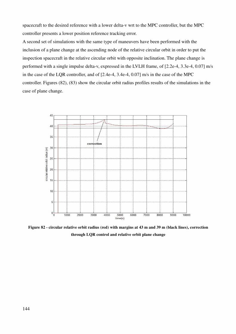
spacecraft to the desired reference with a lower delta-v wrt to the MPC controller, but the MPC
controller presents a lower position reference tracking error.
A second set of simulations with the same type of maneuvers have been performed with the
inclusion of a plane change at the ascending node of the relative circular orbit in order to put the
inspection spacecraft in the relative circular orbit with opposite inclination. The plane change is
performed with a single impulse delta-v, expressed in the LVLH frame, of [2.2e-4, 3.3e-4, 0.07] m/s
in the case of the LQR controller, and of [2.4e-4, 3.4e-4, 0.07] m/s in the case of the MPC
controller. Figures (82), (83) show the circular orbit radius profiles results of the simulations in the
case of plane change.
Figure 82 - circular relative orbit radius (red) with margins at 43 m and 39 m (black lines), correction
through LQR control and relative orbit plane change
144
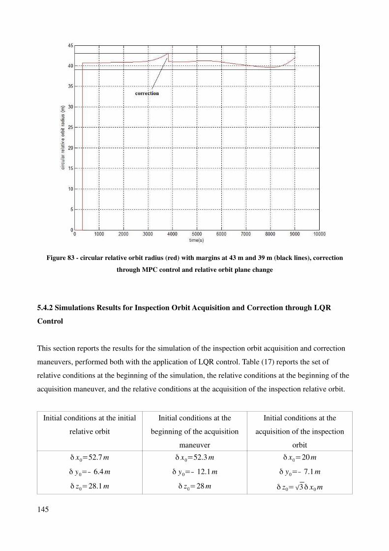
Figure 83 - circular relative orbit radius (red) with margins at 43 m and 39 m (black lines), correction
through MPC control and relative orbit plane change
5.4.2 Simulations Results for Inspection Orbit Acquisition and Correction through LQR
Control
This section reports the results for the simulation of the inspection orbit acquisition and correction
maneuvers, performed both with the application of LQR control. Table (17) reports the set of
relative conditions at the beginning of the simulation, the relative conditions at the beginning of the
acquisition maneuver, and the relative conditions at the acquisition of the inspection relative orbit.
Initial conditions at the initial
relative orbit
Initial conditions at the
beginning of the acquisition
maneuver
Initial conditions at the
acquisition of the inspection
orbit
δ x0=52.7 m
δ y0=− 6.4m
δ z0=28.1 m
δ x0=52.3 m
δ y0=− 12.1m
δ z0=28 m
δ x0=20m
δ y0=− 7.1m
δ z0=√3δ x0 m
145
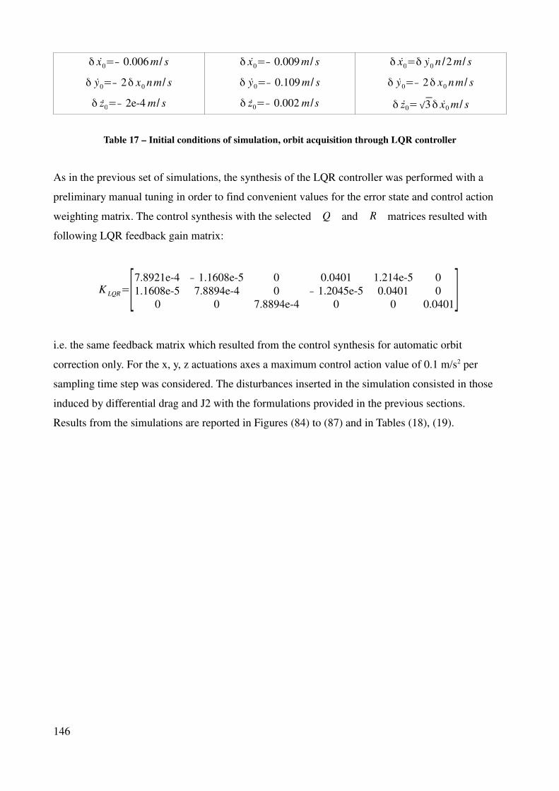
δ x0=− 0.006 m / s
δ y0=− 2δ x0 nm / s
δ z0=− 2e-4 m / s
δ x0=− 0.009m / s
δ y0=− 0.109 m / s
δ z0=− 0.002 m /s
δ x0=δ y0 n /2 m / s
δ y0=− 2δ x0 n m / s
δ z0=√3δ x0 m / s
Table 17 – Initial conditions of simulation, orbit acquisition through LQR controller
As in the previous set of simulations, the synthesis of the LQR controller was performed with a
preliminary manual tuning in order to find convenient values for the error state and control action
weighting matrix. The control synthesis with the selected Q and R matrices resulted with
following LQR feedback gain matrix:
K LQR=[7.8921e-4 − 1.1608e-5 0 0.0401 1.214e-5 0
1.1608e-5 7.8894e-4 0 − 1.2045e-5 0.0401 0
0 0 7.8894e-4 0 0 0.0401]
i.e. the same feedback matrix which resulted from the control synthesis for automatic orbit
correction only. For the x, y, z actuations axes a maximum control action value of 0.1 m/s2 per
sampling time step was considered. The disturbances inserted in the simulation consisted in those
induced by differential drag and J2 with the formulations provided in the previous sections.
Results from the simulations are reported in Figures (84) to (87) and in Tables (18), (19).
146
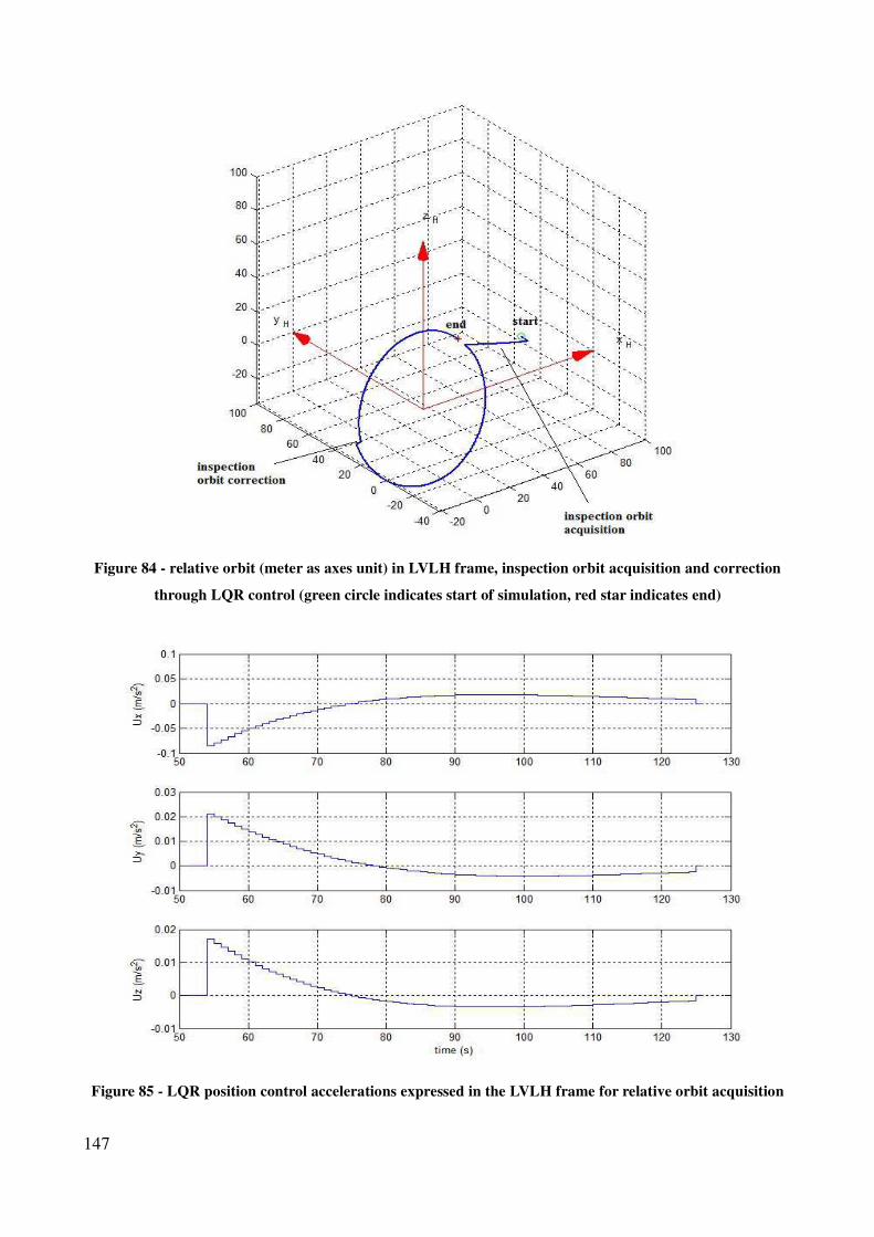
Figure 84 - relative orbit (meter as axes unit) in LVLH frame, inspection orbit acquisition and correction
through LQR control (green circle indicates start of simulation, red star indicates end)
Figure 85 - LQR position control accelerations expressed in the LVLH frame for relative orbit acquisition
147
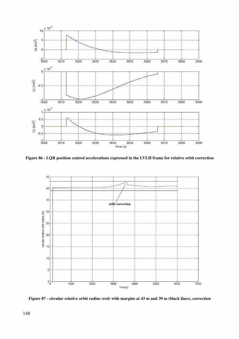
Figure 86 - LQR position control accelerations expressed in the LVLH frame for relative orbit correction
Figure 87 - circular relative orbit radius (red) with margins at 43 m and 39 m (black lines), correction
148
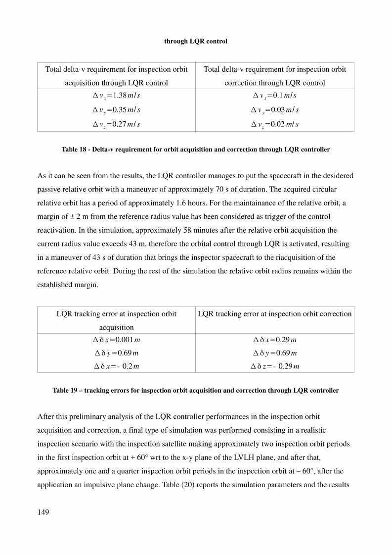
through LQR control
Total delta-v requirement for inspection orbit
acquisition through LQR control
Total delta-v requirement for inspection orbit
correction through LQR control
∆ v x=1.38 m /s
∆ v y=0.35m / s
∆ vz=0.27m / s
∆ v x=0.1 m /s
∆ v y=0.03m / s
∆ vz=0.02 m/ s
Table 18 - Delta-v requirement for orbit acquisition and correction through LQR controller
As it can be seen from the results, the LQR controller manages to put the spacecraft in the desidered
passive relative orbit with a maneuver of approximately 70 s of duration. The acquired circular
relative orbit has a period of approximately 1.6 hours. For the maintainance of the relative orbit, a
margin of ± 2 m from the reference radius value has been considered as trigger of the control
reactivation. In the simulation, approximately 58 minutes after the relative orbit acquisition the
current radius value exceeds 43 m, therefore the orbital control through LQR is activated, resulting
in a maneuver of 43 s of duration that brings the inspector spacecraft to the riacquisition of the
reference relative orbit. During the rest of the simulation the relative orbit radius remains within the
established margin.
LQR tracking error at inspection orbit
acquisition
LQR tracking error at inspection orbit correction
∆ δ x=0.001 m
∆δ y=0.69m
∆δ x=− 0.2 m
∆δ x=0.29 m
∆ δ y=0.69m
∆δ z=− 0.29 m
Table 19 – tracking errors for inspection orbit acquisition and correction through LQR controller
After this preliminary analysis of the LQR controller performances in the inspection orbit
acquisition and correction, a final type of simulation was performed consisting in a realistic
inspection scenario with the inspection satellite making approximately two inspection orbit periods
in the first inspection orbit at + 60° wrt to the x-y plane of the LVLH plane, and after that,
approximately one and a quarter inspection orbit periods in the inspection orbit at – 60°, after the
application an impulsive plane change. Table (20) reports the simulation parameters and the results
149
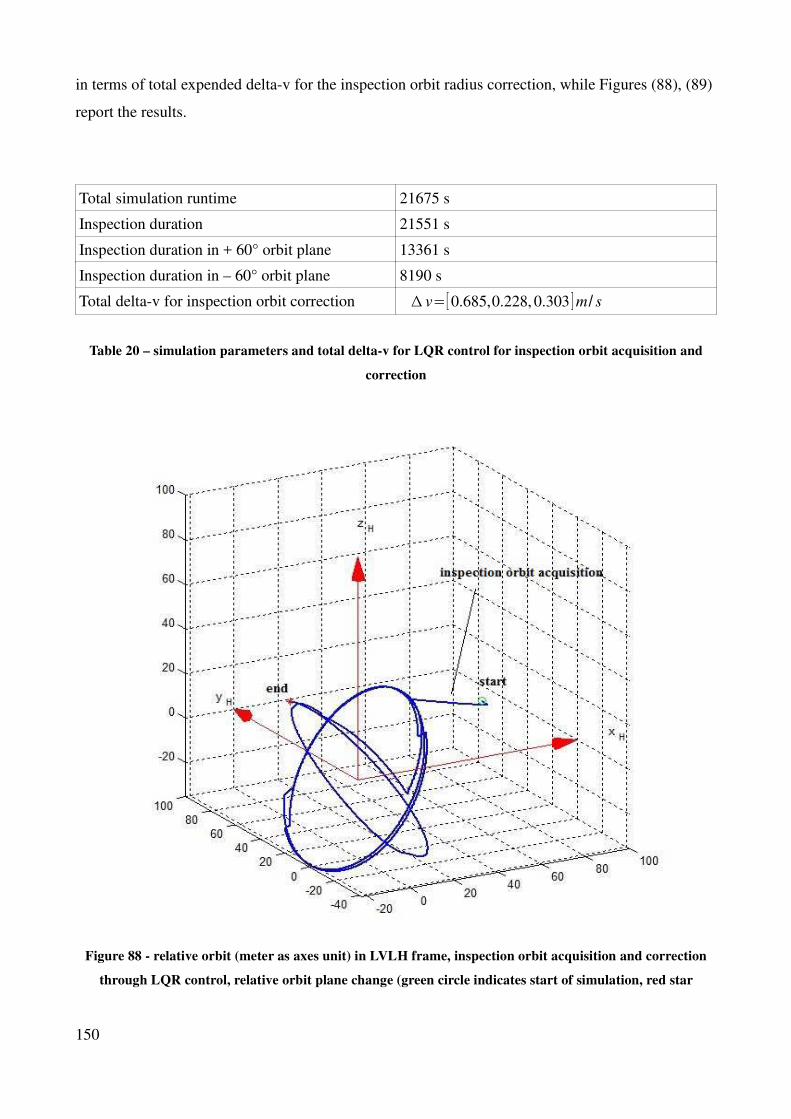
in terms of total expended delta-v for the inspection orbit radius correction, while Figures (88), (89)
report the results.
Total simulation runtime 21675 s
Inspection duration 21551 s
Inspection duration in + 60° orbit plane 13361 s
Inspection duration in – 60° orbit plane 8190 s
Total delta-v for inspection orbit correction ∆ v=[0.685,0.228, 0.303 ]m / s
Table 20 – simulation parameters and total delta-v for LQR control for inspection orbit acquisition and
correction
Figure 88 - relative orbit (meter as axes unit) in LVLH frame, inspection orbit acquisition and correction
through LQR control, relative orbit plane change (green circle indicates start of simulation, red star
150
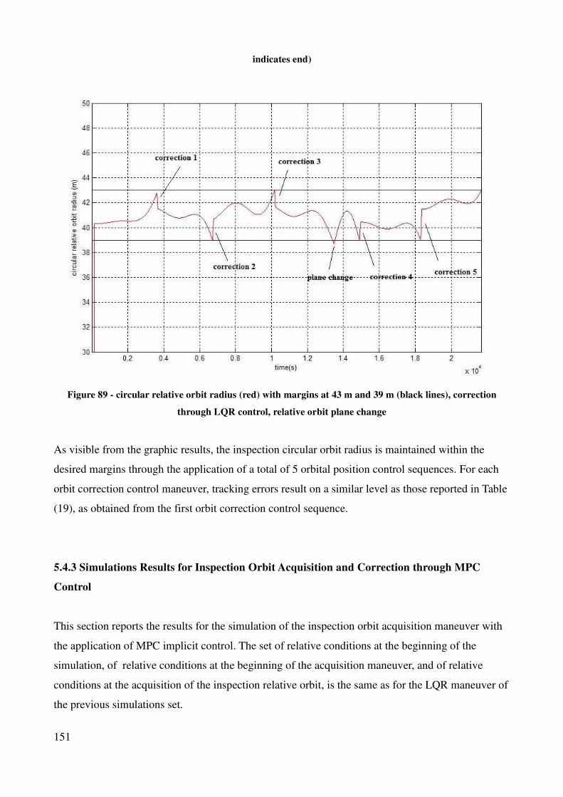
indicates end)
Figure 89 - circular relative orbit radius (red) with margins at 43 m and 39 m (black lines), correction
through LQR control, relative orbit plane change
As visible from the graphic results, the inspection circular orbit radius is maintained within the
desired margins through the application of a total of 5 orbital position control sequences. For each
orbit correction control maneuver, tracking errors result on a similar level as those reported in Table
(19), as obtained from the first orbit correction control sequence.
5.4.3 Simulations Results for Inspection Orbit Acquisition and Correction through MPC
Control
This section reports the results for the simulation of the inspection orbit acquisition maneuver with
the application of MPC implicit control. The set of relative conditions at the beginning of the
simulation, of relative conditions at the beginning of the acquisition maneuver, and of relative
conditions at the acquisition of the inspection relative orbit, is the same as for the LQR maneuver of
the previous simulations set.
151
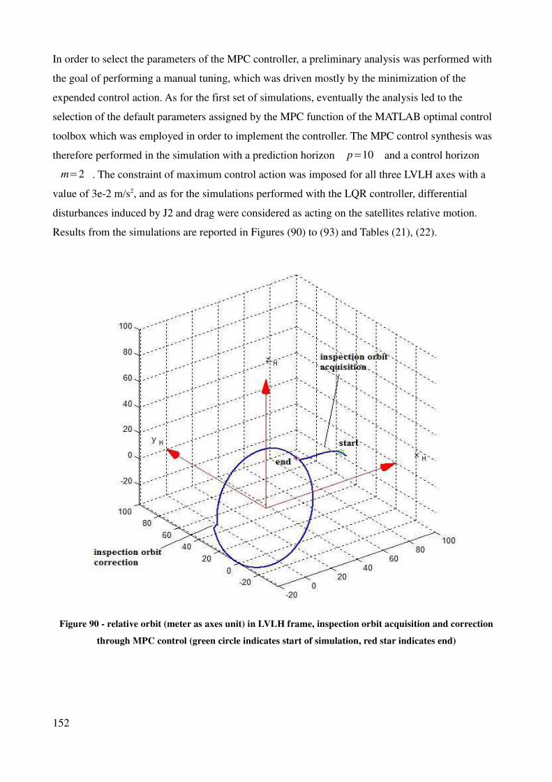
In order to select the parameters of the MPC controller, a preliminary analysis was performed with
the goal of performing a manual tuning, which was driven mostly by the minimization of the
expended control action. As for the first set of simulations, eventually the analysis led to the
selection of the default parameters assigned by the MPC function of the MATLAB optimal control
toolbox which was employed in order to implement the controller. The MPC control synthesis was
therefore performed in the simulation with a prediction horizon p=10 and a control horizon
m=2 . The constraint of maximum control action was imposed for all three LVLH axes with a
value of 3e-2 m/s2, and as for the simulations performed with the LQR controller, differential
disturbances induced by J2 and drag were considered as acting on the satellites relative motion.
Results from the simulations are reported in Figures (90) to (93) and Tables (21), (22).
Figure 90 - relative orbit (meter as axes unit) in LVLH frame, inspection orbit acquisition and correction
through MPC control (green circle indicates start of simulation, red star indicates end)
152
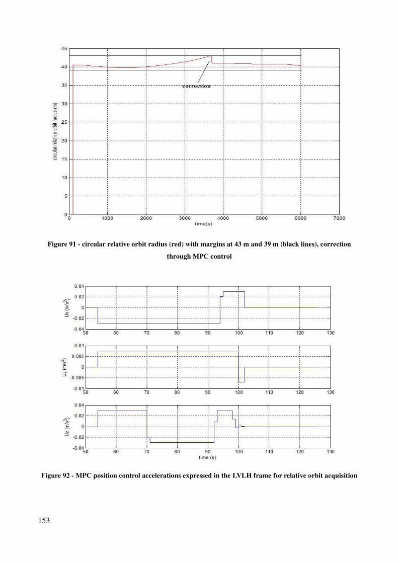
Figure 91 - circular relative orbit radius (red) with margins at 43 m and 39 m (black lines), correction
through MPC control
Figure 92 - MPC position control accelerations expressed in the LVLH frame for relative orbit acquisition
153
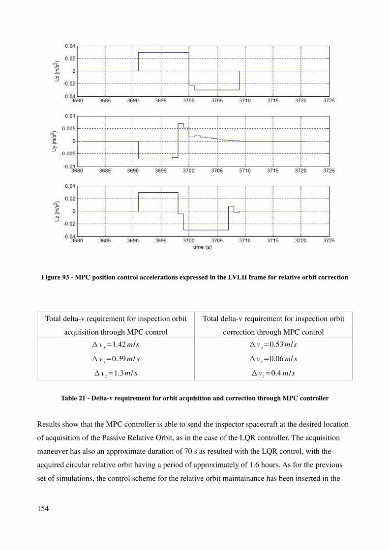
Figure 93 - MPC position control accelerations expressed in the LVLH frame for relative orbit correction
Total delta-v requirement for inspection orbit
acquisition through MPC control
Total delta-v requirement for inspection orbit
correction through MPC control
∆ v x=1.42 m /s
∆ v y=0.39 m / s
∆ vz=1.3m / s
∆ v x=0.53 m /s
∆ v y=0.06 m/ s
∆ vz=0.4 m /s
Table 21 - Delta-v requirement for orbit acquisition and correction through MPC controller
Results show that the MPC controller is able to send the inspector spacecraft at the desired location
of acquisition of the Passive Relative Orbit, as in the case of the LQR controller. The acquisition
maneuver has also an approximate duration of 70 s as resulted with the LQR control, with the
acquired circular relative orbit having a period of approximately of 1.6 hours. As for the previous
set of simulations, the control scheme for the relative orbit maintainance has been inserted in the
154
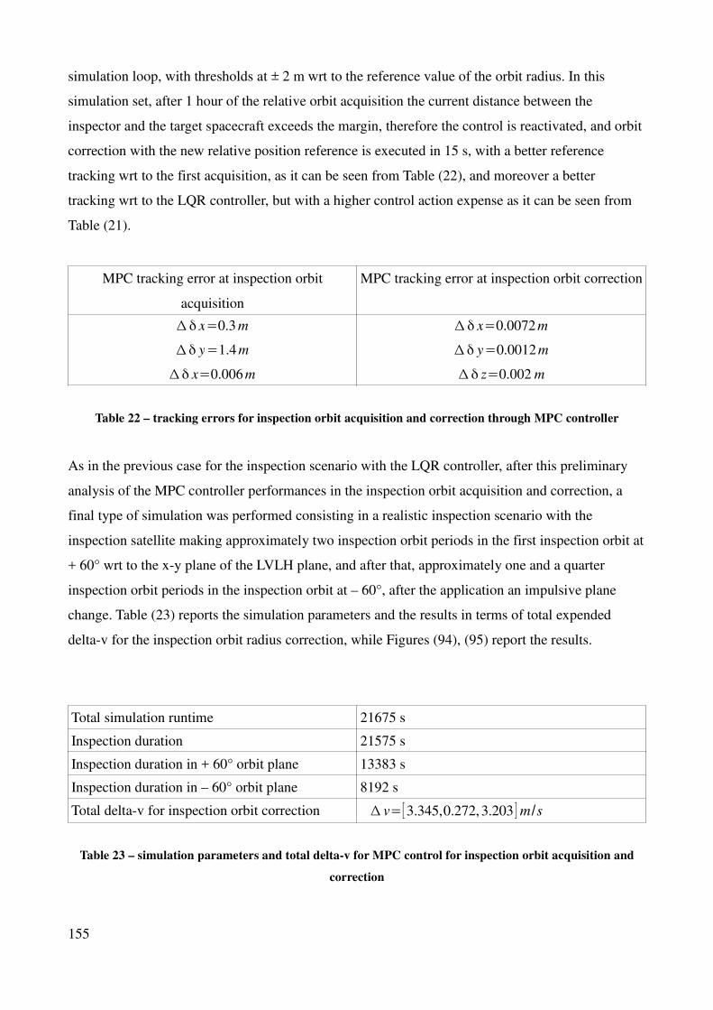
simulation loop, with thresholds at ± 2 m wrt to the reference value of the orbit radius. In this
simulation set, after 1 hour of the relative orbit acquisition the current distance between the
inspector and the target spacecraft exceeds the margin, therefore the control is reactivated, and orbit
correction with the new relative position reference is executed in 15 s, with a better reference
tracking wrt to the first acquisition, as it can be seen from Table (22), and moreover a better
tracking wrt to the LQR controller, but with a higher control action expense as it can be seen from
Table (21).
MPC tracking error at inspection orbit
acquisition
MPC tracking error at inspection orbit correction
∆ δ x=0.3 m
∆δ y=1.4m
∆δ x=0.006 m
∆ δ x=0.0072m
∆δ y=0.0012m
∆δ z=0.002 m
Table 22 – tracking errors for inspection orbit acquisition and correction through MPC controller
As in the previous case for the inspection scenario with the LQR controller, after this preliminary
analysis of the MPC controller performances in the inspection orbit acquisition and correction, a
final type of simulation was performed consisting in a realistic inspection scenario with the
inspection satellite making approximately two inspection orbit periods in the first inspection orbit at
+ 60° wrt to the x-y plane of the LVLH plane, and after that, approximately one and a quarter
inspection orbit periods in the inspection orbit at – 60°, after the application an impulsive plane
change. Table (23) reports the simulation parameters and the results in terms of total expended
delta-v for the inspection orbit radius correction, while Figures (94), (95) report the results.
Total simulation runtime 21675 s
Inspection duration 21575 s
Inspection duration in + 60° orbit plane 13383 s
Inspection duration in – 60° orbit plane 8192 s
Total delta-v for inspection orbit correction ∆ v=[3.345,0.272, 3.203 ]m /s
Table 23 – simulation parameters and total delta-v for MPC control for inspection orbit acquisition and
correction
155
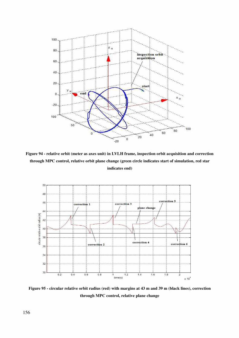
Figure 94 - relative orbit (meter as axes unit) in LVLH frame, inspection orbit acquisition and correction
through MPC control, relative orbit plane change (green circle indicates start of simulation, red star
indicates end)
Figure 95 - circular relative orbit radius (red) with margins at 43 m and 39 m (black lines), correction
through MPC control, relative plane change
156
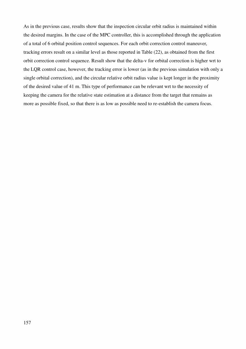
As in the previous case, results show that the inspection circular orbit radius is maintained within
the desired margins. In the case of the MPC controller, this is accomplished through the application
of a total of 6 orbital position control sequences. For each orbit correction control maneuver,
tracking errors result on a similar level as those reported in Table (22), as obtained from the first
orbit correction control sequence. Result show that the delta-v for orbital correction is higher wrt to
the LQR control case, however, the tracking error is lower (as in the previous simulation with only a
single orbital correction), and the circular relative orbit radius value is kept longer in the proximity
of the desired value of 41 m. This type of performance can be relevant wrt to the necessity of
keeping the camera for the relative state estimation at a distance from the target that remains as
more as possible fixed, so that there is as low as possible need to re-establish the camera focus.
157

158
6 CONCLUSIONS
The aim of my Ph.D. Activities has been focused on the development and testing of the cooperating
SPAcecRaft Testbed for Autonomous proximity operatioNs experimentS (SPARTANS) hardware
simulator, under development at the Center of Studies and Activities for Space (CISAS) of the
University of Padova. This ground simulator is made up of robotic units which allow the
reproduction in a controlled environment of the relative position and attitude motions of satellites in
proximity or in formation, and can therefore be used in order to extensively study control
algorithms and strategies for these types of applications, allowing the testing in a controlled
environment of dedicated hardware in the loop. The Units of the simulator have 5 DOF each, 2
translational and 3 rotational, are equipped with a Guidance Navigation and Control (GNC) system
which allows the execution of control maneuvers, and have a communication system which allows
transmission and reception of data and commands between each other and an external control
station consisting of a laptop. This type of testbed allows in particular a good reproduction of the
relative motion of satellites in close proximity maneuvers at low position and attitude relative
velocities, even though in the case of Rendez Vous and Docking or Capture maneuvers simulated
with hardware interfaces the absolute contact forces can not be reproduced at their actual levels. For
the case of proximity maneuvers at higher distances and Satellite Formation Flying the testbed can
be employed for the study of relative maneuvers with scaled control accelerations profiles obtained
from software simulation of the orbital maneuver.
Satellite Formation Flying and Proximity Operations are applications that have gained increasing
interest, as they allow the substitution of a single spacecraft with a system made of multiple
satellites, presenting higher accuracy of payload measurements, increased flexibility, redundancy,
robustness, reduction of development costs, and they allow applications useful for several different
purposes, such as Automated Rendez-Vous and Docking. These systems suffer however from a
generally complicated design since position and attitude control presents both absolute and relative
state requirements, which makes these systems liable to produce high control action expense, since
the control must respond to both relative and absolute references. Moreover, applications like
Automated Rendez-Vous and Docking and in general close proximity maneuvers present a high risk
of impact between satellites. These aspects justify the development and employment of a ground
hardware simulator which allows extensive test sessions with an easily accessible system.
At the beginning of my Ph.D., the testbed consisted in the first prototype of the Attitude Module
(AM), a platform with three controllable DOF of Yaw, Pitch and Roll through a air-thrusters based
control system. A small contribution was given as support to the execution of 3 DOF attitude
159
control maneuvers with the AM. After that, the first activity consisted in the design and
development of the Air suspension system in order to allow the low friction translational motion of
a whole Unit over a test table. Three air skids were tested in the Measurement Laboratory in the
Department of Industrial Engineering, allowing the determination of the autonomy levels of the
suspension system. After this activity, the Translation Module (TM) was designed and developed as
a modular structure, as the lower section of the whole Unit of the testbed, which supports the air
suspension system, the AM, and an on board localization system. The TM was designed in order to
allow a 3 DOF configuration and a 5 DOF configuration. After this activity, a position and Azimuth
localization system based on Optical Flow Sensors (OFS) was developed and tested through an
experimental setup based on a prototype of the TM base. The system was calibrated with rotational
and translational motorized stages mounted one on each other, with the imposition of known
motions. A series of maneuvers were then performed with the same motorized stages assemby in
order to assess the accuracy levels of the system. Purely translational and rotational maneuvers
showed a good accuracy of the OFS system, with max deviations from the imposed trajectory of
approximately 0.1° over an angular range of 40°, and of approximately 1 mm over a translational
range of approximately 100 mm. Combined maneuvers, i.e. translational and rotational maneuvers
in sequence, showed a drift behaviour, with a deviation of the level of 1 cm in planar position, when
a rotation of 90° is imposed after a translation of 5 cm. After that, the OFS system, installed and
calibrated in the TM, was integrated with an external vision system under development in parallel in
the context of the SPARTANS project. Results from tests with the two systems and motions
imposed on the TM through the motorized stages showed a good to fair concordance between the
two navigation system (differences of few mm for position, ± 1° for Azimuth), whereas tests with
manually imposed motions with the TM supported by the air suspension system presented again an
evident drift behaviour both for position and rotation.
A parallel activity consisted in the development of the test table of the Units, designed with a
modular structure, with separate sets of levelable legs sustaining the upper sections on which the
Units can translate.
Another parallel activity consisted in the development of a Matlab Software simulator for the
planning and preliminary verification of position and attitude control maneuvers with the Units of
the testbed, and in the design and development of the Units test table. The simulator was employed
for the preliminary planning of 3 DOF attitude and position control maneuvers with standard and
optimal controllers.
The last activity of my Ph.D. consisted in the analysis of an inspection scenario with satellite
removal purposes, with the goal of reproducing the relative dynamics in scale with the SPARTANS
160
simulator. The chosen scenario foresaw the inspection of the freely tumbling Envisat spacecraft in
Low Earth Orbit (LEO). The analysis was focused on the acquisition and maintainance of a circular
relative orbit for the inspection through a satellite, with an approximate range of 40 m, starting from
a flyaround orbit. The analysis was performed with a Matlab orbital software simulator which
integrates the Hill-Clohessy-Wiltshire equations, through the employment of Model Predictive
Control (MPC) and Linear Quadratic Regulator (LQR) controllers for the acquisition and the
maintainance of the inspection orbit, with the implementation of an automatic orbit correction
scheme with triggering margins. Results showed that during all the inspection both LQR and MPC
controllers are able to keep the relative orbit radius within the established margin of ± 2 m: this is
done with lower control action spent by the LQR (max total delta-v component of 0.7 m/s for a total
of 5 orbital correction sequences) wrt to the MPC, but with a higher tracking error, resulting in the
circular orbit radius being more unstable and for less time close to the desired value, wrt to the
MPC results, which in turn presented a max total delta-v component of 3.3 m/s for a total of 6
orbital correction sequences.
Activities in the immediate future will consist in the assembly of the Test Table, assembly of the
second prototype of the AM and of the first complete Unit of the testbed, and development and
testing of the vision-based navigation system for the estimation of the 5 DOF Unit dynamic state in
an absolute external frame of reference. This will allow the execution of a first series of attitude and
position control maneuvers with a single Unit, employing simulated virtual targets for the execution
of coordinated control maneuvers. In its final form the SPARTANS simulator will present a
minimum of two Units performing coordinated control maneuvers for the simulation of Satellite
Formation Flying, Automated Rendez-Vous and Docking, and other proximity maneuvers with
hardware in the loop.
161

162
Bibliography
[1] W. H. Clohessy and R. S. Wiltshire, "Terminal Guidance System for Satellite Rendez-Vous",
Journal of the Aerospace Sciences, vol. 27, no. 1, pp. 653-658, 1960
[2] J. Leitner, "Formation Flying - The Future of Remote Sensing from Space", Proceedings of the
18th International Symposium on Space Flight Dynamics (ESA SP-548), 11-15 October 2004,
Munich, Germany.
[3] D. Scharf, F. Hadaegh, and S. R. Ploen, "A Survey of Spacecraft Formation Flying Guidance
and Control (Part I): Guidance," Proceedings of the American Control Conlerence, 4-6 June 2003,
Denver, Colorado.
[4] D. P. Scharf, F. Y. Hadaegh, and S. Ploen,"A Survey of Spacecraft Formation Flying Guidance
and Control (Part II): Control," Proceedings of 2004 the American Control Conlerence, June 30 -
July 2 2004, Boston, Massachusetts.
[5] G. Krieger, M. Zink, M. Bachmann, B. Bräutigam, D. Schulze, M. Martone, P. Rizzoli,
U. Steinbrecher, J. W. Antony, F. De Zan, I. Hajnsek, K. Papathanassiou, F. Kugler, M. R. Cassola,
M. Younis, S. Baumgartner, P. Lopez-Dekker, P. Prats, and A. Moreira, "TanDEM-X: a radar
interferometer with two formation-fying satellites", Acta Astronautica, vol. 89, no. 0, pp. 83 - 98,
2013.
[6] J. L. Schwartz, M. A. Peck, and C. D. Hall, "Historical Review of Air-Bearing Spacecraft
Simulators," Journal of Guidance, Control and Dynamics, vol. 26, no. 4, pp. 513- 522, July-August
2003.
[7] J. P. M. O. Hilstad and A. G. Richards, The SPHERES Guest Scientist Program. Space Systems
Laboratory, Massachusetts Institute of Technology, 2009.
[8] A. Valmorbida, F. Scarpa, M. Mazzucato, S. Tronco, S. Debei and E. C. Lorenzini, “Attitude
Module Characterization of the Satellite Formation Flight Testbed”, Proceedings of the IEEE
International Workshop on Metrology for Aerospace, May 29-30, 2014, Benevento, Italy
163

[9] A. Valmorbida, M. Mazzucato, A. Aboudan and S. Tronco, “Test of Attitude Control Maneuvers
with a Satellite Formation Flight Testbed”, Proceedings of the IEEE International Workshop on
Metrology for Aerospace, May 29-30, 2014, Benevento, Italy
[10] Valmorbida A., Mazzucato M., Tronco S., Debei S., Lorenzini E. C., “SPARTANS – a
cooperating spacecraft testbed for autonomous proximity operations experiments”, Instrumentation
and Measurement Technology Conference (I2MTC), 2015 IEEE International, Pisa, Italy
[11] Mazzucato M., Tronco S., Valmorbida A., Scibona F., Lorenzini E. C., “Development of a
ground based cooperating spacecraft testbed for research and education”, 1st Symposium on Space
Educational activities, December 9-11 2015, Padova, Italy
[12] Valmorbida A., Tronco S., Mazzucato M., Debei S., Lorenzini E. C., “Optical flow sensor
based localization system for a cooperating spacecraft testbed”, IEEE Metrology for Aerospace
2015, Benevento, Italy
[13] A. Bonarini, M. Matteucci, and M. Restelli, "A Kinematic Independent Dead-reckoning
Sensor for Indoor Mobile Robotics", Proceedings of the 2004 IEEE/RSJ Conference on Intelligent
Robotics ans Systems, September 28 – October 2, 2004, Sendai, Japan.
[14] D. Miller, A. Saenz-Otero, J. Wertz, A. Chen, G. Berkowski, C. Brodel, S. Carlson, D.
Carpenter, S. Chen, S. Cheng, D. Feller, S. Jackson, B. Pitts, F. Perez, J. Szuminski and S. Sell,
“SPHERES: A Testbed for Long Duration Satellite Formation Flying In Micro-Gravity Conditions,”
Proceedings of the AAS/AIAA Space Flight Mechanics Meeting, Clearwater, FL, USA, Jan. 23-26,
2000, AAS 00-110.
[15] M. Schlotterer and S. Theil, "Testbed for on-orbit servicing and formation flying dynamics
emulation", AIAA Guidance, Navigation, and Control Conference, 2 - 5 August 2010, Toronto,
Ontario, Canada.
[16] S. Bell, “High Precision Robot Odometry Using an Array of Optical Mouse”, Oklahoma
Christian University colloquium paper, 2011. Available at:
http://stanford.edu/~sebell/oc_projects.html.
164
[17] H. Schaub and J. L. Junkins, Analytical Mechanics of Space Systems. American Institute of
Aeronautics and Astronautics Inc., 2003.
[18] K. T. Alfriend, S. R. Vadali, P. Gurl, J. P. How, and L. S. Breger, Spacecraft Formation Flying:
Dynamics, control and navigation. Butterworth-Heinemann, 1st edition 2010.
[19] D. A. Vallado, Fundamentals of Astrodynamics and Applications. Microcosm Press/Springer,
3rd edition 2007.
[20] P. Ferguson and J. How, "Decentralized Estimation Algorithms for Formation Flying
Spacecraft," in the AIAA Guidance, Navigation and Control Conference, pp. 2003- 5442, 2003.
[21] A. Visioli, Practical PID Control. Springer, 2006.
[22] J. M. Maciejowski, Predictive Control with Constraints. Prentice Hall, 2002.
[23] J. A. Rossiter, Model-Based Predictive Control - A Practical Approach. CRC Press, 2003.
[24] D. Q. Mayne, J. B. Rawlings, C. V. Rao, and P. O. M. Scokaert,"Constrained Model Predictive
Control: Stability and optimality", Automatica, vol. 36, pp. 789-814, 2000.
[25] Y.-G. Xi, D.-W. LI, and S. LIN, "Model Predictive Control - Status and Challenges", Acta
Automatica Sinica, vol. 39, no. 3, 2013.
[26] J. H. Lee, "Model Predictive Control: Review of the Three Decades of Development",
International Journal of Control, Automation and Systems, vol. 9, no. 3, pp. 415 - 424, 2011.
[27] J. B. Rawlings, "Tutorial Overview of Model Predictive Control", IEEE Control System Mag-
azine, pp. 38 - 52, June 2000.
[28] A. Bemporad, M. Morari, V. Dua, and E. N. Pistikopoulos, "The explicit linear quadratic
regulator for constrained systems", Automatica, vol. 38, pp. 3 - 20, 2002.
[29] Mazzucato M., Valmorbida A., Tronco S., Costantini M., Debei S., Lorenzini E. C.,
165
“ Development of a camera-aided optical mouse sensors based localization system for a free
floating planar robot”, IEEE Metrology for Aerospace 2016, Firenze, Italy
[30] L. Kneip, D. Scaramuzza, R. Siegwart, "A Novel Parametrization of the Perspective-Three-
Point Problem for a Direct Computation of Absolute Camera Position and Orientation", Proc. IEEE
Conf. on Computer Vision and Pattern Recognition, CVPR 2011.
[31] Pertile, M.; Mazzucato, M.; Bottaro, L.; Chiodini, S.; Debei, S.; Lorenzini, E., ”Uncertainty
evaluation of a vision system for pose measurement of a spacecraft with fiducial markers,” in
Metrology for Aerospace (MetroAeroSpace), 2015 IEEE , vol., no., pp.283-288, 4-5 June 2015
[32] M. A. Fischler and R. C. Bolles. Random sample consensus: a paradigm for model fitting with
applications to image analysis and automated cartography. Commun. ACM, Vol. 24, Nr.6, pp.381 -
395, 1981.
[33] R. E. Kalman, "A New Approach to Linear Filtering and Prediction Problems," Transaction
of the ASME - Journal of Basic Engineering, pp. 35 - 45, 1960.
[34] D. Sekimori and F. Miyazaki, ”Self-localization for indoor mobile robots based on optical
mouse sensor values and simple global camera information,” 2005 IEEE International Conference
on Robotics and Biomimetics - ROBIO, Shatin, 2005, pp. 605-610. doi:
10.1109/ROBIO.2005.246337.
[35] Feng Yu, Zhen He, Bing Qiao, Xiaoting Yu, "Stereo Vision Based Relative Pose Estimation for
the Rendezvous and Docking of Noncooperative Satellites", Mathematical Problems in
Engineering, Volume 2014 (2014), Article ID 461283
[36] Schweighart, S. A., & Sedwick, R. J. (2002). High-Fidelity Linearized J2 Model for Satellite
Formation Flight. Journal of Guidance, Control and Dynamics,Vol. 25, No.6, pp. 1073-1080.
[37] Silva, E. D. (2008). A Formulation of the Clohessy-Wiltshire Equations to Include Dynamic
Atmospheric Drag. Paper presented at the AIAA/AAS Astrodynamics Specialist Conference.
[38] Guangyan Xu, Tingting Yu, Jianchao Wang, Xia Chen, "Model Predictive Control of Passive
166

and Periodic Satellite Formation Based on Linear Programming Approach", Proceedings of 2014
IEEE Chinese Guidance, Navigation and Control Conference, August 8-10 2014, Yantai, China
167