Embed Size (px)
Citation preview

Dottorato di Ricerca in Ingegneriadell’Informazione
XX CICLO
Sede Amministrativa di ModenaUniversita degli studi di MODENA e REGGIO EMILIA
TESI PER IL CONSEGUIMENTO DEL TITOLO DIDOTTORE DI RICERCA
Self-Adaptive distributed systemsfor Internet-based services
Candidata:Ing. Sara Casolari
Relatore:Prof. Michele Colajanni


“La science avec des faits comme une maison avec despierres; mais une accumulation de faits n’est pas plusune science qu’un tas de pierres n’est une maison.”
“La scienza e fatta di dati come una casa di pietre.Ma un ammasso di dati none scienza piu di quanto unmucchio di pietre sia una casa.”
“Science is made of data as a house is made of stones.But a mass of data is not science more han a pile ofstones is a house.”
Jules-Henri Poincare


Contents
1 Introduction 17
2 Statistical properties of the internal resource measures 232.1 Correlation analysis . . . . . . . . . . . . . . . . . . . . . . . . . 252.2 Spectral and noise analysis . . . . . . . . . . . . . . . . . . . . . 282.3 Heteroscedasticity . . . . . . . . . . . . . . . . . . . . . . . . . . 322.4 Auto-correlation . . . . . . . . . . . . . . . . . . . . . . . . . . . 332.5 Summary . . . . . . . . . . . . . . . . . . . . . . . . . . . . . . 35
3 Multi-phase methodology 373.1 Proposal . . . . . . . . . . . . . . . . . . . . . . . . . . . . . . . 37
3.1.1 Representative resource load . . . . . . . . . . . . . . . . 393.1.2 Resource state interpretation . . . . . . . . . . . . . . . . 393.1.3 Runtime decision systems . . . . . . . . . . . . . . . . . 41
3.2 Internet-based systems . . . . . . . . . . . . . . . . . . . . . . . 413.2.1 Case study: test-bed system . . . . . . . . . . . . . . . . 423.2.2 Workload models . . . . . . . . . . . . . . . . . . . . . . 433.2.3 Resource measures . . . . . . . . . . . . . . . . . . . . . 49
4 Load tracker models 534.1 Definitions . . . . . . . . . . . . . . . . . . . . . . . . . . . . . . 53
4.1.1 Linear load trackers . . . . . . . . . . . . . . . . . . . . . 554.1.2 Non-linear load trackers . . . . . . . . . . . . . . . . . . 57
4.2 Evaluation methods for load trackers . . . . . . . . . . . . . . . .594.2.1 Computational cost . . . . . . . . . . . . . . . . . . . . . 604.2.2 Accuracy and responsiveness . . . . . . . . . . . . . . . . 60
4.3 Results . . . . . . . . . . . . . . . . . . . . . . . . . . . . . . . . 634.3.1 Accuracy . . . . . . . . . . . . . . . . . . . . . . . . . . 634.3.2 Responsiveness . . . . . . . . . . . . . . . . . . . . . . . 674.3.3 Precision . . . . . . . . . . . . . . . . . . . . . . . . . . 684.3.4 Statistical analysis of the load trackers . . . . . . . . . .. 70
6 CONTENTS
4.4 Significance of the results . . . . . . . . . . . . . . . . . . . . . . 714.5 Self-adaptive load tracker . . . . . . . . . . . . . . . . . . . . . . 74
5 Load change detection 795.1 Problem definition . . . . . . . . . . . . . . . . . . . . . . . . . 805.2 Algorithms for load change detection . . . . . . . . . . . . . . . .81
5.2.1 Single threshold-based scheme . . . . . . . . . . . . . . . 815.2.2 CUSUM scheme . . . . . . . . . . . . . . . . . . . . . . 82
5.3 Evaluation: reactivity and delay error . . . . . . . . . . . . . .. 835.4 Results . . . . . . . . . . . . . . . . . . . . . . . . . . . . . . . . 86
5.4.1 Single threshold . . . . . . . . . . . . . . . . . . . . . . 865.4.2 CUSUM . . . . . . . . . . . . . . . . . . . . . . . . . . 88
5.5 Conclusions . . . . . . . . . . . . . . . . . . . . . . . . . . . . . 90
6 Load trend 936.1 Problem definition . . . . . . . . . . . . . . . . . . . . . . . . . 93
6.1.1 Qualitative behavior . . . . . . . . . . . . . . . . . . . . 946.1.2 Quantitative behavior . . . . . . . . . . . . . . . . . . . . 956.1.3 Positioning . . . . . . . . . . . . . . . . . . . . . . . . . 96
6.2 Load trend applications . . . . . . . . . . . . . . . . . . . . . . . 976.3 Weighted-Trend Algorithm . . . . . . . . . . . . . . . . . . . . . 99
7 Load prediction 1017.1 Problem definition . . . . . . . . . . . . . . . . . . . . . . . . . 1027.2 Linear prediction models . . . . . . . . . . . . . . . . . . . . . . 1067.3 Trend-aware regression prediction model . . . . . . . . . . . .. . 1087.4 Results . . . . . . . . . . . . . . . . . . . . . . . . . . . . . . . . 111
7.4.1 Predictability . . . . . . . . . . . . . . . . . . . . . . . . 1117.4.2 Quality of the prediction models . . . . . . . . . . . . . . 1147.4.3 Sensitivity analysis . . . . . . . . . . . . . . . . . . . . . 118
7.5 Conclusions . . . . . . . . . . . . . . . . . . . . . . . . . . . . . 120
8 Applications 1238.1 Web cluster . . . . . . . . . . . . . . . . . . . . . . . . . . . . . 1238.2 Locally distributed Network Intrusion Detection System . . . . . 1288.3 Geographically distributed Web-based system . . . . . . . .. . . 1328.4 Multi-tier Web system . . . . . . . . . . . . . . . . . . . . . . . 135
9 Related work 1399.1 Internal vs. external system view . . . . . . . . . . . . . . . . . . 1399.2 Observed resource measures vs. load representation . . .. . . . . 141

CONTENTS 7
9.3 Realistic Internet-based context . . . . . . . . . . . . . . . . . .. 1429.4 Off-line models vs. runtime model . . . . . . . . . . . . . . . . . 143
10 Conclusions 147

List of Figures
2.1 Observed data set. . . . . . . . . . . . . . . . . . . . . . . . . . . 242.2 Examples of correlation analysis results . . . . . . . . . . . .. . 272.3 Scatter plot between the external view (number of arrivals) and
internal view (server utilization). . . . . . . . . . . . . . . . . . . 282.4 Spectral analysis of the internal resource measures. . .. . . . . . 302.5 Heteroscedasticity of the internal resource measures.. . . . . . . 332.6 Auto-correlation function of the internal resource measures . . . . 34
3.1 The proposed multi-phase framework for supporting runtime de-cisions. . . . . . . . . . . . . . . . . . . . . . . . . . . . . . . . 38
3.2 Typical architecture of a Web-based system . . . . . . . . . . .. 423.3 Architecture of the considered multi-tier Web-based system . . . . 433.4 User section class diagram. . . . . . . . . . . . . . . . . . . . . . 463.5 Syntheticuser scenarios (the number of emulated browsers refers
to the heavy service demand) . . . . . . . . . . . . . . . . . . . . 483.6 Realisticuser scenarios (the number of emulated browsers refers
to the heavy service demand) . . . . . . . . . . . . . . . . . . . . 483.7 Resource measurements - light service demand. . . . . . . . .. . 493.8 Resource measurements - heavy service demand. . . . . . . . .. 493.9 Statistical analysis of the workloads. . . . . . . . . . . . . . .. . 513.10 Boxplot of the performance indexes of the resources in stable sce-
nario with light service demand . . . . . . . . . . . . . . . . . . . 523.11 Boxplot of the performance indexes of the resources in realistic
scenario with heavy service demand . . . . . . . . . . . . . . . . 52
4.1 First-phase of the multi-phase framework. . . . . . . . . . . .. . 544.2 Load trackers classification. . . . . . . . . . . . . . . . . . . . . . 554.3 Representative load intervals. . . . . . . . . . . . . . . . . . . . .624.4 Representative load intervals for different user scenarios andlight
service demand. . . . . . . . . . . . . . . . . . . . . . . . . . . . 64
10 LIST OF FIGURES
4.5 Representative load intervals for different user scenarios andheavyservice demand. . . . . . . . . . . . . . . . . . . . . . . . . . . . 64
4.6 Accuracyof the load trackers for the realistic user scenario andheavy service demand (n denotes the number of measured valuesused by a load tracker). . . . . . . . . . . . . . . . . . . . . . . . 65
4.7 Responsivenessof the load trackers for the realistic scenario andheavy service demand. . . . . . . . . . . . . . . . . . . . . . . . 65
4.8 Load tracker curves with respect to representative loadintervals(realistic user scenario and heavy service demand). . . . . . .. . 66
4.9 Accuracyof the load trackers for three user scenarios and lightservice demand. . . . . . . . . . . . . . . . . . . . . . . . . . . . 68
4.10 Responsivenessof the load trackers for three user scenarios andheavy service demand. . . . . . . . . . . . . . . . . . . . . . . . 68
4.11 Scatter plot of the load trackers for the realistic scenario and heavyservice demand. . . . . . . . . . . . . . . . . . . . . . . . . . . . 70
4.12 Scatter plot of the load trackers for the step scenario and lightservice demand. . . . . . . . . . . . . . . . . . . . . . . . . . . . 70
4.13 Heteroscedasticity analysis of the load tracker values vs. the ob-served data set. . . . . . . . . . . . . . . . . . . . . . . . . . . . 72
4.14 Autocorrelation function of the load tracker values. .. . . . . . . 724.15 Flow chart of a self-adaptive load tracker. . . . . . . . . . .. . . 754.16 Comparison betweenadaptiveandself-adaptiveload trackers. . . 774.17 Observed data set and representative load intervals (realistic user
scenario with light service demand). . . . . . . . . . . . . . . . . 784.18 Self-adaptive load tracker and representative load intervals (real-
istic user scenario with light service demand). . . . . . . . . . .. 78
5.1 Second-phase of the multi-phase framework -load change detection. 795.2 Load change detector based on thresholdχ = 0.4 . . . . . . . . . 85
6.1 Second-phase of the multi-phase framework -load trend analysis. 946.2 Qualitative behavior of the geometric interpretation .. . . . . . . 956.3 Resources behavior . . . . . . . . . . . . . . . . . . . . . . . . . 98
7.1 Second-phase of the multi-phase methodology -load prediction. . 1017.2 Auto-correlation functions of the observed data set (measures get
from system monitors). . . . . . . . . . . . . . . . . . . . . . . . 1057.3 Auto-correlation function of the filtered data set. . . . .. . . . . . 1057.4 Trend coefficients form = 4 historical values. . . . . . . . . . . . 1107.5 Auto-correlation functions of the observed data set. . .. . . . . . 112
LIST OF FIGURES 11
7.6 Auto-correlation functions for two load trackers with “adequate”precision (light service demand). . . . . . . . . . . . . . . . . . . 112
7.7 Auto-correlation functions for two load trackers with “adequate”precision (heavy service demand). . . . . . . . . . . . . . . . . . 112
7.8 Scatter plot of the traditional prediction models in realistic sce-nario in heavy service demand. . . . . . . . . . . . . . . . . . . . 117
7.9 Scatter plot of the TAR prediction model in realistic scenario inheavy service demand. . . . . . . . . . . . . . . . . . . . . . . . 117
7.10 Qualitative analysis of the average delay for representing the re-source behavior . . . . . . . . . . . . . . . . . . . . . . . . . . . 118
7.11 Prediction error as a function of the noise index (δ) . . . . . . . . 1217.12 Prediction error as a function of the prediction window(k) . . . . 1217.13 Prediction error as a function of the parameters of the TAR model 121
8.1 Third-phase of the multi-phase framework - runtime decision sys-tem. . . . . . . . . . . . . . . . . . . . . . . . . . . . . . . . . . 124
8.2 Architecture of the multi-tier Web cluster . . . . . . . . . . .. . 1258.3 Number of refused requests during the entire experiment. . . . . . 1278.4 Architecture of the distributed NIDS . . . . . . . . . . . . . . . .1298.5 Load on NIDS traffic analyzers when load balancing is based on
observed data sets . . . . . . . . . . . . . . . . . . . . . . . . . . 1308.6 Load on NIDS traffic analyzers when load balancing is based on
the proposed multi-phase framework (SMA10 load tracker) . . . . 1308.7 Load on NIDS traffic analyzers when load balancing is based on
the proposed multi-phase framework (EMA30 load tracker) . . . . 1308.8 Cumulative distributions of the Coefficient of Variation of the load
on the traffic analyzers. . . . . . . . . . . . . . . . . . . . . . . . 1318.9 Geographically distributed system for the content adaptation. . . . 1338.10 Cumulative distribution of the response time for a geographically
distributed Web-based system supporting content-adaptation ser-vices. . . . . . . . . . . . . . . . . . . . . . . . . . . . . . . . . 134
8.11 Web system architecture . . . . . . . . . . . . . . . . . . . . . . 1358.12 Load balancing in the stable scenario. . . . . . . . . . . . . . .. 1378.13 Load balancing in the realistic scenario. . . . . . . . . . . .. . . 137


List of Tables
2.1 Noise analysis of resource utilization of an Internet-based server . 31
3.1 Service access frequencies (TPC-W workload) for light and heavyservice demand models. . . . . . . . . . . . . . . . . . . . . . . . 45
4.1 CPU time (msec) for the computation of a load tracker value . . . 614.2 Ranges of feasibility. . . . . . . . . . . . . . . . . . . . . . . . . 76
5.1 False detections (step scenario and light service demand) . . . . . 865.2 False detections (staircase scenario and light servicedemand) . . . 875.3 False detections (alternating scenario and light service demand) . 885.4 False detections (realistic scenario and heavy servicedemand) . . 885.5 False detections (Light service demand) - CUSUM algorithm with
static threshold . . . . . . . . . . . . . . . . . . . . . . . . . . . 895.6 False detections (Step scenario and light service demand) - CUSUM
algorithm with Kullback-Leibler threshold . . . . . . . . . . . . .90
6.1 Load trend models . . . . . . . . . . . . . . . . . . . . . . . . . 97
7.1 Auto-correlation values . . . . . . . . . . . . . . . . . . . . . . . 1137.2 Prediction error - prediction windowk = 30 . . . . . . . . . . . . 1157.3 Average delay (sec.) . . . . . . . . . . . . . . . . . . . . . . . . . 119
8.1 Evaluation of the two admission control mechanisms . . . .. . . 1268.2 Evaluation of load balancing mechanisms . . . . . . . . . . . . .1328.3 Performance evaluation of the dispatching algorithms.. . . . . . . 138


Acknowledgements
Desidero ringraziare innanzitutto il Prof. Michele Colajanni per la disponibilita
e la fiducia accordatami, per i preziosi suggerimenti ed il tempo trascorso a ra-
gionare insieme, per la pazienza e l’indispensabile supporto umano.
Se i ragazzi del WEBLAB non si fossero rivelati cosı disponibili ad accettarmi
fra di loro e a mettermi a disposizione cio di cui avevo bisogno, ora non saremmo
giunti ad un risultato cosı soddisfacente: un grazie di cuore. Con particolare af-
fetto dico grazie a Claudia Canali e Alessandro Bulgarelli perche mi hanno fatto
vedere quanto in realta dietro alle apparenti postazioni fredde di un ufficio si pos-
sano scoprire persone umanamente stupende.
Uno speciale e sincero ringraziamento va a tutti coloro che in questi anni
hanno contributo alla mia crescita formativa; tra questi ungrazie particolare va
a Novella Bartolini, Francesco Lo Presti e Simone Silvestri.
Non so se esistano abbastanza parole per ringraziare il rimpianto Prof. Claudio
Canali, che mi ha spronato ad intraprendere un percorso che prima di lui mi sem-
brava inarrivabile, che e stato un esempio per la passione che ha sempre mostrato
nei confronti del proprio lavoro e per l’amore nei confrontidegli studenti.
Per la comprensione, il sostegno e l’incoraggiamento che non mi sono mai
venuti a mancare durante tutto il mio periodo di dottorato, ringrazio tutta la mia
famiglia.
A tutti gli amici e ai compagni di universita: a loro va il ringraziamento piu
grande per aver alleggerito il peso di tante situazioni difficili.
Infine desidero rivolgere un ringraziamento speciale a GianBattista che ha
accompagnato ogni mio passo, con il quale ho condiviso soddisfazioni e delusioni,
che mi ha spronato di fronte ad ogni dubbio e senza il quale questa esperienza non
avrebbe avuto lo stesso sapore.

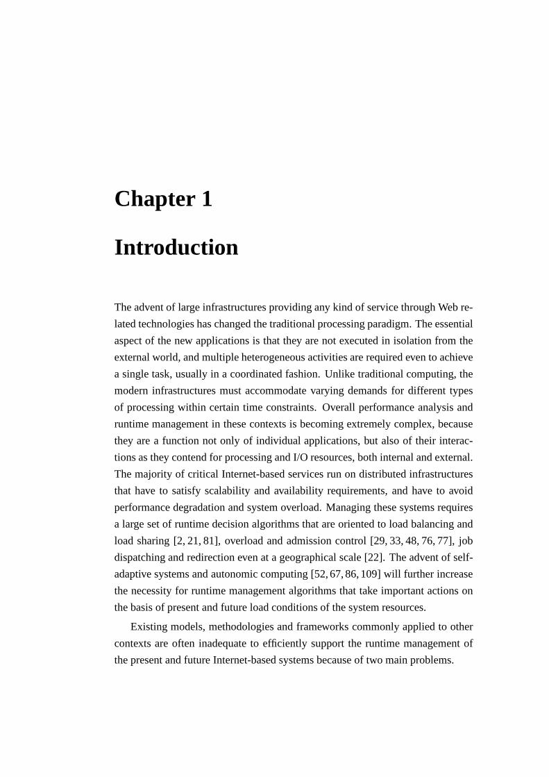
Chapter 1
Introduction
The advent of large infrastructures providing any kind of service through Web re-
lated technologies has changed the traditional processingparadigm. The essential
aspect of the new applications is that they are not executed in isolation from the
external world, and multiple heterogeneous activities arerequired even to achieve
a single task, usually in a coordinated fashion. Unlike traditional computing, the
modern infrastructures must accommodate varying demands for different types
of processing within certain time constraints. Overall performance analysis and
runtime management in these contexts is becoming extremelycomplex, because
they are a function not only of individual applications, butalso of their interac-
tions as they contend for processing and I/O resources, bothinternal and external.
The majority of critical Internet-based services run on distributed infrastructures
that have to satisfy scalability and availability requirements, and have to avoid
performance degradation and system overload. Managing these systems requires
a large set of runtime decision algorithms that are orientedto load balancing and
load sharing [2, 21, 81], overload and admission control [29, 33, 48, 76, 77], job
dispatching and redirection even at a geographical scale [22]. The advent of self-
adaptive systems and autonomic computing [52, 67, 86, 109] will further increase
the necessity for runtime management algorithms that take important actions on
the basis of present and future load conditions of the systemresources.
Existing models, methodologies and frameworks commonly applied to other
contexts are often inadequate to efficiently support the runtime management of
the present and future Internet-based systems because of two main problems.

18 Introduction
• The large majority of the literature related to the Internet-based systems pro-
poses decision systems that are oriented to the analysis of theexternal work-
load and its statistical properties (e.g., heavy-tailed distributions [5, 8, 28],
bursty arrivals [59] and hot spots [10]). Unlike existing models and schemes
oriented to evaluate system performance through a prevalent external traffic
view, in this thesis we propose an originalinternal view.
• Most available algorithms and mechanisms for runtime decisions evaluate
the load conditions of a system through the periodic sampling of resource
measuresobtained from monitors and use these values (or simple combina-
tions of them) as a basis for determining the present and the future system
condition. In this thesis, we propose an innovativemulti-phasemethodol-
ogy that is based on stochastic representations of the resource measures and
on more accurate models for positioning the present and future state of the
system resources with respect to their capacities.
External traffic reaching an Internet-based system shows some time-space pe-
riodic behavior that facilitates its interpretation and management. These char-
acteristics are extremely useful for capacity planning andsystem dimensioning
goals, but they are useless to estimate a precise status of aninternal resource be-
cause we will demonstrate that they are not clearly correlated with the arrivals at
an Internet-based system. An external view that is quite predominant in the state
of the art, tends to not deal with the complexity and mostly unknown statistics of
the system internals supporting modern Internet-based system. Consequently, an
external system view has little or no possibility of really controlling the complex-
ity of these modern processing models and their inter-dependencies. We claim
that for taking adequate runtime decisions, we should be able to describe modern
Internet-based services in terms of internal system scenarios consisting of numer-
ous I/O streams, timing information, and interactive concurrent tasks that enter
and leave the system in a way that is difficult to predict. In this thesis, we present
statistical analyses and propose mathematical models based on an internal system
view that is useful to pave the way toadaptiveandself-adaptiveways of taking
runtime management decisions. Anadaptivesystem evaluates statically its own
global behavior and changes it when the evaluation indicates that it is not accom-
19
plishing what it was intended to do, or when better functionality or performance
is possible. Aself-adaptivesystem evaluates dynamically the behavior of every
component and is able to take autonomous decisions with low or null interaction
with the other components.
Adaptiveandself-adaptivesystems seem an inevitable mean to manage the
increasing complexity of present and future Internet-based information systems
that have to satisfy scalability and availability requirements, have to avoid per-
formance degradation and system overload and have to identify when and how
to change specific behaviors to achieve the desired improvement. For example,
taking autonomous decisions according to some objective rules for event detec-
tion or for triggering actions concerning data/service placement but also to detect
overloaded or faulty components, requires the ability of automatically capturing
significant information about the internal state of the resources and also adapting
the monitoring system to internal and external conditions.
In other more traditional contexts [1, 10, 31], resource measures are valid
sources to decide about where the system is, where the systemis going, whether
is it necessary to activate some management process. While ameasure offers an
instantaneous view of the load conditions of a resource, in the typical context of
the Web workload and distributed Internet-based systems, it is of little help for
distinguishing overload conditions from transient peaks,for understanding load
trends and for anticipating future conditions, that are of utmost importance for
taking correct decisions. Another problem that our analyses confirm is that the
resource measures referring to Internet-based servers areextremely variable even
at different time scales, and tend to become obsolete ratherquickly [39].
As an alternative, we propose that decision systems operateon a continuous
“representation” of the load behavior of system resources.This idea leads to a
multi-phase methodologywhere we separate the problem of achieving a repre-
sentative view of the system conditions from that of using this representation for
runtime decision purposes. In this thesis, we propose and compare models and
mechanisms that are necessary to support any runtime decision in an Internet-
based system foradaptiveandself-adaptiveapplications: monitoring, measure-
ment and sampling, algorithms for extracting useful information from rough data,
ability of adapting the monitoring system to internal and external conditions.

20 Introduction
The research activities have several innovative goals thatwe will detail in the
following nine chapters.
1. We carry out the first accurate analysis of the stochastic runtime behav-
ior of the internal resources measures of the system belonging to different
Internet-based architectures (Chapter 2).
2. We present an innovativemulti-phase methodology. This methodology has
a general validity because it is independent of the user behavior and can be
extended to many different contexts (Chapter 3).
3. We propose and compare different linear and non-linear functions, called
laod trackers, that generateadaptiveand self-adaptiverepresentations of
the resource load that are suitable to support different decision systems and
are characterized by a computational complexity that is compatible with the
temporal constraints of runtime decisions. These functions get continuous
resource measures from the system monitors, evaluate a loadrepresentation
of one or multiple resources, and pass this representation to the functions of
the second phase (Chapter 4).
4. We utilize the load representations obtained through theprevious load track-
ers to develop innovative stochastic models for supportingsome fundamen-
tal tasks characterizing runtime management decisions in Internet-based
systems, such as:
• load change detectionfor signaling non-transient changes of the load
conditions of a system resource (Chapter 5);
• load trend analysisthat is useful to characterize the behavior of the
system in a significant past (Chapter 6).
• load predictionfor anticipating future load conditions of the system
(Chapter 7);
5. We propose novel runtime decision systems that are based on the previ-
ous stochastic models, for some classic problems characterizing distributed

21
Internet-based systems, such asload balancing, admission controlandre-
quests redirection. Moreover, we integrate themulti-phase methodology
into frameworks that are applied to different prototypes ofdistributed In-
ternet systems consisting of multiple servers, such as a Webcluster, a ge-
ographically distributed architecture, a distributed Intrusion Detection Sys-
tem (Chapter 8).
6. We compare the main results of this thesis against the state of the art in
Chapter 9 and we conclude with some future work research lines in Chap-
ter 10.


Chapter 2
Statistical properties of the internalresource measures
In this chapter we propose a detailed analysis of the statistical behavior of the
most important internalresource measuresof Internet-based systems. We con-
sider these measures or samples asstochastic data setsthat are continuously pro-
vided by the system monitors. A data set is an ordered collection of n data, begin-
ning at timeti−(n−1) and covering events up to a final timeti. Specifically, we have
Xn(ti) = [xi−(n−1), . . . , xi−1, xi], where thej-th elementxj , i − n + 1 ≤ j ≤ i,
denotes the value of one or more resource measures of interest, whereas the index
j indicates its time of occurrence,tj . The elements ofXn(ti) are time-ordered,
that is, tj ≤ tz for any j < z. As an example, assume that a system moni-
tor captures the CPU utilization every ten seconds during anobservation interval
of thirty minutes. In this case, the historical informationconsists of(xi)i=1,...,n,
wheren = 180, xi is the CPU utilization at timeti, and the time increases in steps
of ten seconds.
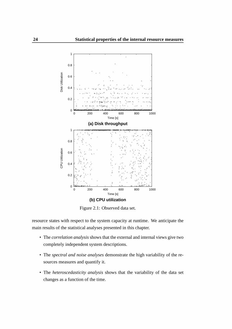
Figure 2.1 reports the typical behavior of two data sets obtained from the mon-
itoring of two internal resources CPU and disk utilization of an Internet-based
server node. From the direct observation of these internal resources measures, it
is impossible to understand where the system load really is and where it is going.
The properties and the characteristics of the data sets coming from the in-
ternal views of Internet-based servers are a quite new field that requires further
investigations for achieving a useful interpretation an adequate positioning of the
24 Statistical properties of the internal resource measures
0
0.2
0.4
0.6
0.8
1
0 200 400 600 800 1000
Dis
k U
tiliz
atio
n
Time [s]
(a) Disk throughput
0
0.2
0.4
0.6
0.8
1
0 200 400 600 800 1000
CP
U U
tiliz
atio
n
Time [s]
(b) CPU utilization
Figure 2.1: Observed data set.
resource states with respect to the system capacity at runtime. We anticipate the
main results of the statistical analyses presented in this chapter.
• Thecorrelation analysisshows that the external and internal views give two
completely independent system descriptions.
• Thespectral and noise analysesdemonstrate the high variability of the re-
sources measures and quantify it.
• The heteroscedasticity analysisshows that the variability of the data set
changes as a function of the time.

2.1 Correlation analysis 25
• Theauto-correlation analysisdemonstrates a significant time independence
of the observed resource measures that prevents their predictability.
2.1 Correlation analysis
The correlation is a statistical property that aims to understand whether a some
sort of relationship between two data sets exists. Our first goal is to evaluate the
correlation between the internal and external system views. If a strong relation-
ship existed, the proposed internal system view would be useless because both
views would be able to provide the same status information. On the other hand,
a scarce correlation shows that the two views capture different information about
the system and the proposed approach is well motivated.
In mathematical terms, thecorrelation coefficientindicates the strength and
direction of a linear relationship between two random data sets. There are several
coefficients for measuring the degree of correlation that depends on the nature of
the data. The most popular index is the Pearson product-moment correlation coef-
ficient [66], which is obtained by dividing the covariance ofthe two random data
sets by the product of their standard deviations. Hence, we can write the correla-
tion coefficientρXn(ti),Yn(ti) between two random data setsXn(ti) andYn(ti) with
expected valuesµXn(ti)andµYn(ti) and standard deviationsσXn(ti) andσYn(ti) as:
ρXn(ti),Yn(ti) =Cov(Xn(ti), Yn(ti))
σXn(ti)σYn(ti)=
E((Xn(ti) − µXn(ti))(Yn(ti) − µYn(ti)))
σXn(ti)σYn(ti),
(2.1)
whereE is the expected value operator andCov denotes the covariance between
the two random data sets.
SinceµXn(ti) = E(Xn(ti)), σ2Xn(ti)
= E(Xn(ti)2)−E2(Xn(ti)) and similarly
for Yn(ti), we may also write the Equation 2.1 as:
ρXn(ti),Yn(ti) =E(Xn(ti)Yn(ti)) − E(Xn(ti))E(Yn(ti))
√
E(Xn(ti)2) − E2(Xn(ti))√
E(Yn(ti)2) − E2(Yn(ti)). (2.2)
The correlation coefficient is 1 in case of an increasing linear relationship, -1
in case of a decreasing linear relationship, and some value between -1 and 1 in
26 Statistical properties of the internal resource measures
all the other instances that indicate some degree of linear dependence between
the two data sets. The closer the coefficient is to either -1 or1, the stronger the
correlation between the data sets.
If the data sets are independent, then their correlation is 0. The opposite is
false, because the correlation coefficient detects only linear dependencies between
two data sets. For example, suppose the random data setXn(ti) is uniformly
distributed on the interval from -1 to 1, andYn(ti) = Xn(ti)2. ThenYn(ti) is
completely determined byXn(ti), so thatXn(ti) andYn(ti) are dependent, but
their correlation is zero, hence they are uncorrelated. However, in the special case
whenXn(ti) andYn(ti) are jointly normal, an uncorrelated behavior is equivalent
to an independent behavior. A correlation between two data sets is reduced in
presence of noisy measurements of one or both data sets. In these cases, filtering
or smoothing techniques guarantee a more accurate coefficient.
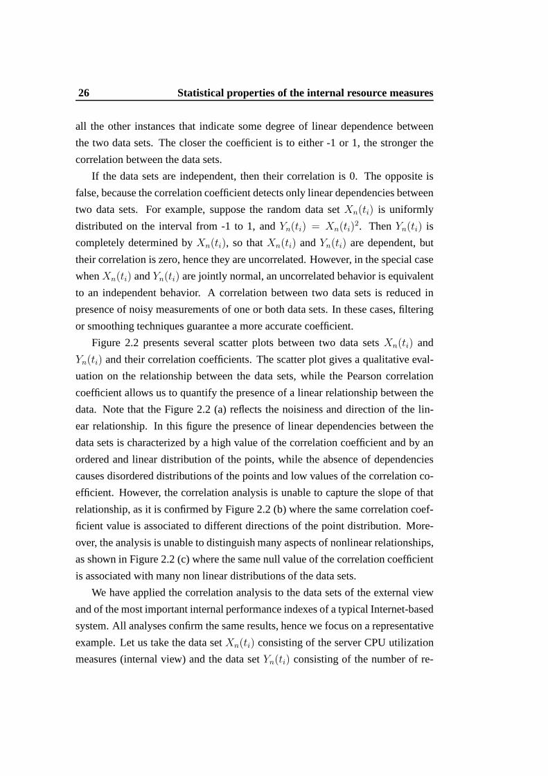
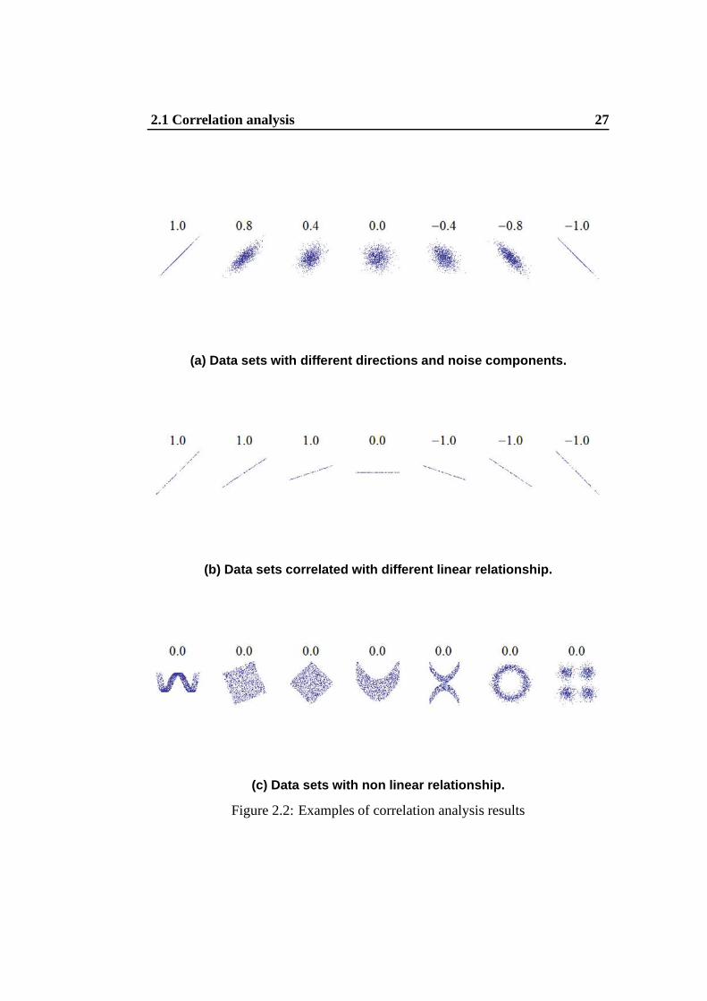
Figure 2.2 presents several scatter plots between two data sets Xn(ti) and
Yn(ti) and their correlation coefficients. The scatter plot gives aqualitative eval-
uation on the relationship between the data sets, while the Pearson correlation
coefficient allows us to quantify the presence of a linear relationship between the
data. Note that the Figure 2.2 (a) reflects the noisiness and direction of the lin-
ear relationship. In this figure the presence of linear dependencies between the
data sets is characterized by a high value of the correlationcoefficient and by an
ordered and linear distribution of the points, while the absence of dependencies
causes disordered distributions of the points and low values of the correlation co-
efficient. However, the correlation analysis is unable to capture the slope of that
relationship, as it is confirmed by Figure 2.2 (b) where the same correlation coef-
ficient value is associated to different directions of the point distribution. More-
over, the analysis is unable to distinguish many aspects of nonlinear relationships,
as shown in Figure 2.2 (c) where the same null value of the correlation coefficient
is associated with many non linear distributions of the datasets.
We have applied the correlation analysis to the data sets of the external view
and of the most important internal performance indexes of a typical Internet-based
system. All analyses confirm the same results, hence we focuson a representative
example. Let us take the data setXn(ti) consisting of the server CPU utilization
measures (internal view) and the data setYn(ti) consisting of the number of re-
2.1 Correlation analysis 27
(a) Data sets with different directions and noise component s.
(b) Data sets correlated with different linear relationshi p.
(c) Data sets with non linear relationship.
Figure 2.2: Examples of correlation analysis results
28 Statistical properties of the internal resource measures
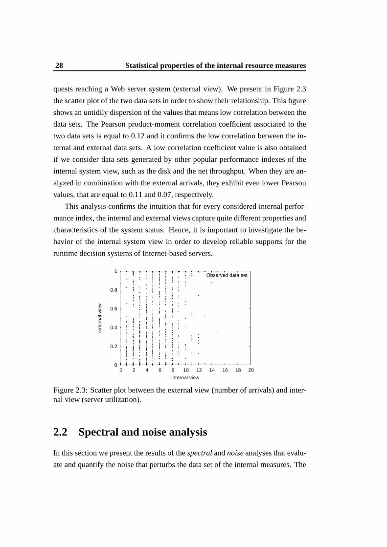
quests reaching a Web server system (external view). We present in Figure 2.3
the scatter plot of the two data sets in order to show their relationship. This figure
shows an untidily dispersion of the values that means low correlation between the
data sets. The Pearson product-moment correlation coefficient associated to the
two data sets is equal to 0.12 and it confirms the low correlation between the in-
ternal and external data sets. A low correlation coefficientvalue is also obtained
if we consider data sets generated by other popular performance indexes of the
internal system view, such as the disk and the net throughput. When they are an-
alyzed in combination with the external arrivals, they exhibit even lower Pearson
values, that are equal to 0.11 and 0.07, respectively.
This analysis confirms the intuition that for every considered internal perfor-
mance index, the internal and external views capture quite different properties and
characteristics of the system status. Hence, it is important to investigate the be-
havior of the internal system view in order to develop reliable supports for the
runtime decision systems of Internet-based servers.
0
0.2
0.4
0.6
0.8
1
0 2 4 6 8 10 12 14 16 18 20
exte
rnal
vie
w
internal view
Observed data set
Figure 2.3: Scatter plot between the external view (number of arrivals) and inter-nal view (server utilization).
2.2 Spectral and noise analysis
In this section we present the results of thespectralandnoiseanalyses that evalu-
ate and quantify the noise that perturbs the data set of the internal measures. The

2.2 Spectral and noise analysis 29
spectral analysisbreaks a signal in the time domain into all of its individual fre-
quency components. It allows to separate thelow frequency component, that is the
un-noise signal, from thehigh frequency component, that is the noise. On the other
hand, thenoise analysisallows us to quantify the high frequency components.
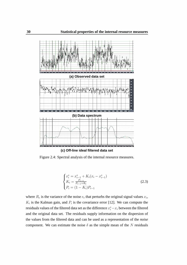
From the Figure 2.4 (a), we can see that a high dispersion of the values char-
acterizes the measurements of the internal resource indexes during the entire ob-
servation period. A highly variable and noisy data set (showing a so called jittery
behavior) limits the ability of taking adequate decisions in distributed systems
supporting Internet-based services.
We can give a mathematical confirmation of the dispersion of values shown
in Figure 2.4 (a) by evaluating thespectral analysisof the resource measurement
values. Figure 2.4 (b) reports the data spectrum of the observed data set of Fig-
ure 2.4 (a). In Figure 2.4 (b), we can see that the noise that perturbs the signal is
uniformly distributed in the entire frequency domain. Whenthe noise component
presents this characteristic, it is defined aswhite noiseand shows an uncorrelated
behavior between all instantaneous values. Every signal that presents white noise
appears completely unpredictable with respect to the previous values [25]. We
should recall that these observations, which are detailed for a specific data set, are
valid for all the considered internal resources of an Internet-based system. How-
ever, if we carry out an off-line analysis of the data set through an ideal filter, we
can show the possibility of achieving a ”clean” curve (Figure 2.4 (c)) from the
original perturbed signal. This result gives some foundations to themulti-phase
methodology presented in Chapter 3, although we should remark that we are in-
terested to runtime filtering and not to off-line analyses.
We are interested not only to demonstrate the presence of noise in the observed
data sets, but we also want to quantify the noise perturbation for all the considered
performance indexes. For thenoise analysis, we consider the Kalman Filter, that is
the optimal linear estimator to evaluate the on-lineidealfiltered data setX∗n(ti) =
(x∗i−(n−1), . . . , x
∗i ) referring to the observed data set. We assume that in the filtered
data set, thej-th element (i − n + 1 ≤ j ≤ i) is denoted by the filtered valuex∗j .
The considered Kalman filter is:
30 Statistical properties of the internal resource measures
(a) Observed data set
(b) Data spectrum
(c) Off-line ideal filtered data set
Figure 2.4: Spectral analysis of the internal resource measures.
x∗i = x∗
i−1 + Ki(xi − x∗i−1)
Ki = Pi−1
Pi−1+Re
Pi = (1 − Ki)Pi−1
(2.3)
whereRe is the variance of the noiseet that perturbs the original signal valuesxi,
Ki is the Kalman gain, andPi is the covariance error [12]. We can compute the
residuals values of the filtered data set as the differencex∗i −xi between the filtered
and the original data set. The residuals supply informationon the dispersion of
the values from the filtered data and can be used as a representation of thenoise
component. We can estimate the noiseδ as the simple mean of theN residuals
2.2 Spectral and noise analysis 31
generated by theidealfilters:
δ =
∑
i(x∗
i −xi)
x∗
i
)
N(2.4)
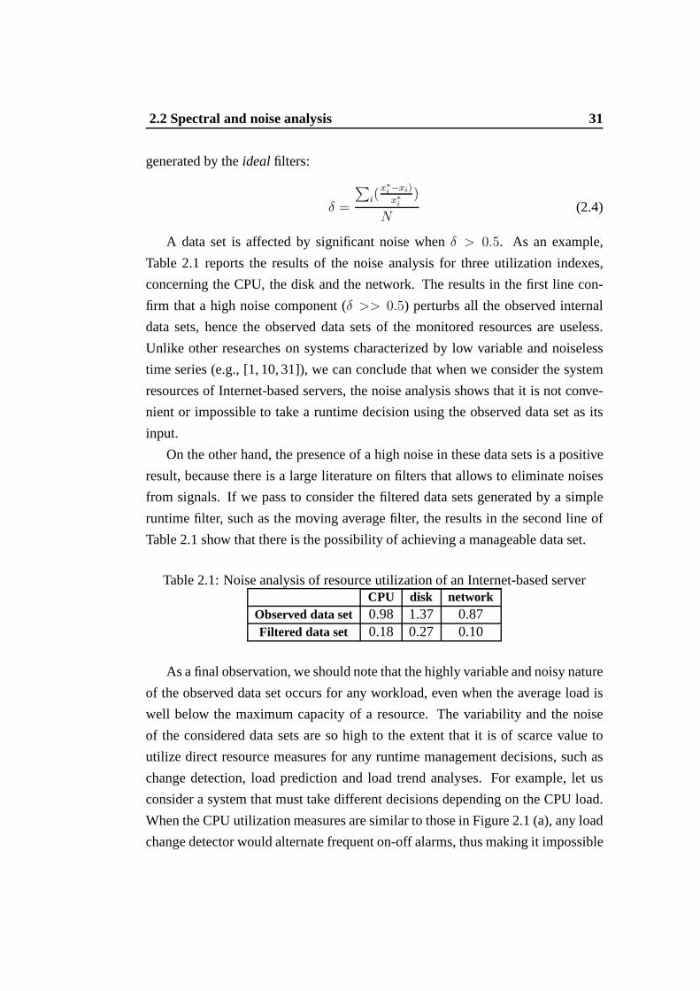
A data set is affected by significant noise whenδ > 0.5. As an example,
Table 2.1 reports the results of the noise analysis for threeutilization indexes,
concerning the CPU, the disk and the network. The results in the first line con-
firm that a high noise component (δ >> 0.5) perturbs all the observed internal
data sets, hence the observed data sets of the monitored resources are useless.
Unlike other researches on systems characterized by low variable and noiseless
time series (e.g., [1, 10, 31]), we can conclude that when we consider the system
resources of Internet-based servers, the noise analysis shows that it is not conve-
nient or impossible to take a runtime decision using the observed data set as its
input.
On the other hand, the presence of a high noise in these data sets is a positive
result, because there is a large literature on filters that allows to eliminate noises
from signals. If we pass to consider the filtered data sets generated by a simple
runtime filter, such as the moving average filter, the resultsin the second line of
Table 2.1 show that there is the possibility of achieving a manageable data set.
Table 2.1: Noise analysis of resource utilization of an Internet-based serverCPU disk network
Observed data set 0.98 1.37 0.87Filtered data set 0.18 0.27 0.10
As a final observation, we should note that the highly variable and noisy nature
of the observed data set occurs for any workload, even when the average load is
well below the maximum capacity of a resource. The variability and the noise
of the considered data sets are so high to the extent that it isof scarce value to
utilize direct resource measures for any runtime management decisions, such as
change detection, load prediction and load trend analyses.For example, let us
consider a system that must take different decisions depending on the CPU load.
When the CPU utilization measures are similar to those in Figure 2.1 (a), any load
change detector would alternate frequent on-off alarms, thus making it impossible

32 Statistical properties of the internal resource measures
to a runtime decision system to judge whether a node is reallyoff-loaded or not.
On the other hand, a simple average of the resource measures would mitigate
the on-off effect, but at the expenses of the efficacy of the load change detection
algorithm.
2.3 Heteroscedasticity
The spectraland noiseanalyses confirm and quantify the presence of a noise
component that perturbs the original data sets of the internal resources measures of
an Internet-based system. However, these analyses do not give us any information
about the time variability of the data set, while it is usefulto know whether it is
constant or changes with time. If the data set variability remains constant, the
filtering technique that reduces the noise component does not require any update.
On the other hand, for a continuously variable data set, the filtering technique
needs frequent adaptations in order to guarantee a reduced noise component.
We analyze theheteroscedasticity propertyto describe the characteristics of
the data set variability. A random data set is heteroscedastic if the random vari-
ables have different variances [100, 108]. To verify this property, we use the
Breusch-Pagan test [15] that first evaluates a linear regression model describing
the data set, then computes the residuals from the data set and the corresponding
regression model values, and lastly tests whether the estimated variance of the
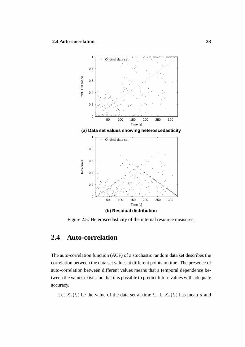
residuals is dependent on the values of the data set. Figure 2.5 shows a graphical
representation of heteroscedasticity on a data set of internal resource measures. In
particular, Figure 2.5 (a) reports the variable dispersionof the values in a period
of 330 observations and the linear regression model (the black dotted line). The
residuals distribution, shown in Figure 2.5 (b), points outa variable behavior and
confirms the presence of heteroscedasticity. From this test, we evince that the in-
ternal resource measures of a typical Internet-based system are characterized by
heteroscedasticity. This result confirms the difficulties of obtaining a reliable view
of the state of an Internet-based system and the necessity ofproposing filters that
are able to self-adapt their parameters to the changeable variances of the data set
in order to eliminate the noise component.
2.4 Auto-correlation 33
0
0.2
0.4
0.6
0.8
1
50 100 150 200 250 300
CP
U U
tiliz
atio
n
Time [s]
Original data set
(a) Data set values showing heteroscedasticity
0
0.2
0.4
0.6
0.8
1
50 100 150 200 250 300
Res
idua
ls
Time [s]
Original data set
(b) Residual distribution
Figure 2.5: Heteroscedasticity of the internal resource measures.
2.4 Auto-correlation
The auto-correlation function (ACF) of a stochastic randomdata set describes the
correlation between the data set values at different pointsin time. The presence of
auto-correlation between different values means that a temporal dependence be-
tween the values exists and that it is possible to predict future values with adequate
accuracy.
Let Xn(ti) be the value of the data set at timeti. If Xn(ti) has meanµ and
34 Statistical properties of the internal resource measures
varianceσ2, then the definition of the ACF is:
R(Xn(ti), Xn(ti+k)) =E[(Xn(ti) − µ)(Xn(ti+k) − µ)]
σ2(2.5)
whereE is the expected value operator. This expression is not well-defined for
all data set values, since the varianceσ2 may be zero (for a constant data set) or
infinite for most heavy-tailed distributions. If the function R is well defined, its
value must lie in the range[−1, 1], with 1 indicating perfect correlation and−1
indicating perfect anti-correlation. When the data set is highly variable, typically
there is a limited possibility of predicting future values and future states of the
system and its auto-correlation value is low.
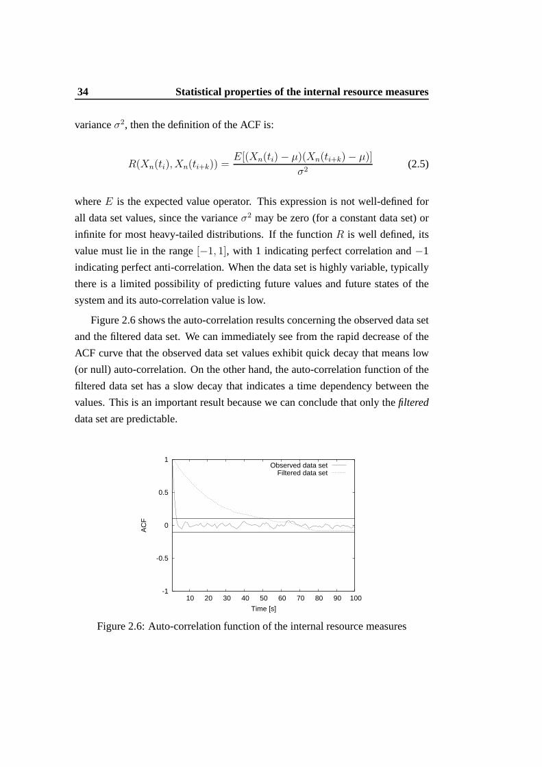
Figure 2.6 shows the auto-correlation results concerning the observed data set
and the filtered data set. We can immediately see from the rapid decrease of the
ACF curve that the observed data set values exhibit quick decay that means low
(or null) auto-correlation. On the other hand, the auto-correlation function of the
filtered data set has a slow decay that indicates a time dependency between the
values. This is an important result because we can conclude that only thefiltered
data set are predictable.
-1
-0.5
0
0.5
1
10 20 30 40 50 60 70 80 90 100
AC
F
Time [s]
Observed data setFiltered data set
Figure 2.6: Auto-correlation function of the internal resource measures
2.5 Summary 35
2.5 Summary
In this chapter we have proposed a mathematical and statistical description of typ-
ical data sets referring to internal resource measures of anInternet-based system.
The statistical properties of the observed data sets evidence:
• very low correlation between the internal and the externalsystem view;
• high dispersion of the observed values;
• high noise component;
• a significant heteroscedastisity;
• low or null auto-correlation.
These results, carried out on real system data, demonstratethat a runtime de-
cision system cannot operate on observed data sets, but we should find a differ-
ent representation of the resource load that guarantees lownoise component, ho-
moscedastic behavior and a time dependency between the values. This research
will be the focus of the next chapters.


Chapter 3
Multi-phase methodology
3.1 Proposal
In Chapter 2, we have demonstrated that observed data sets have a limited util-
ity because they offer just instantaneous views about the load conditions of a
resource. Moreover, they tend to be useless when they are highly variable and
perturbed by a noise component. It is practically impossible to estimate and pre-
dict load state, to analyze load state trend, to forecast overload, to decide whether
it is necessary or not to activate some control mechanism and, in case, to choose
the right action.
For these reasons, we propose that runtime management systems supporting
adaptiveandself-adaptiveInternet-based services should operate not on observed
data sets but on a continuous “representation” of the load behavior that should be
able to adapt itself to the workload and system variations. This proposal leads to a
multi-phase methodologythat separates the complex management decisions pro-
cesses of an Internet-based system in three main phases, as outlined in Figure 3.1.
1. Generation of representative resource load.During this phase, we obtain
“representative” views of the resource load through the support of stochastic
models.
2. Resource state interpretation. In this phase, we propose some mecha-
nisms that use the previous representation as a basis for evaluating impor-
tant information about the present (e.g., load change detection), the future
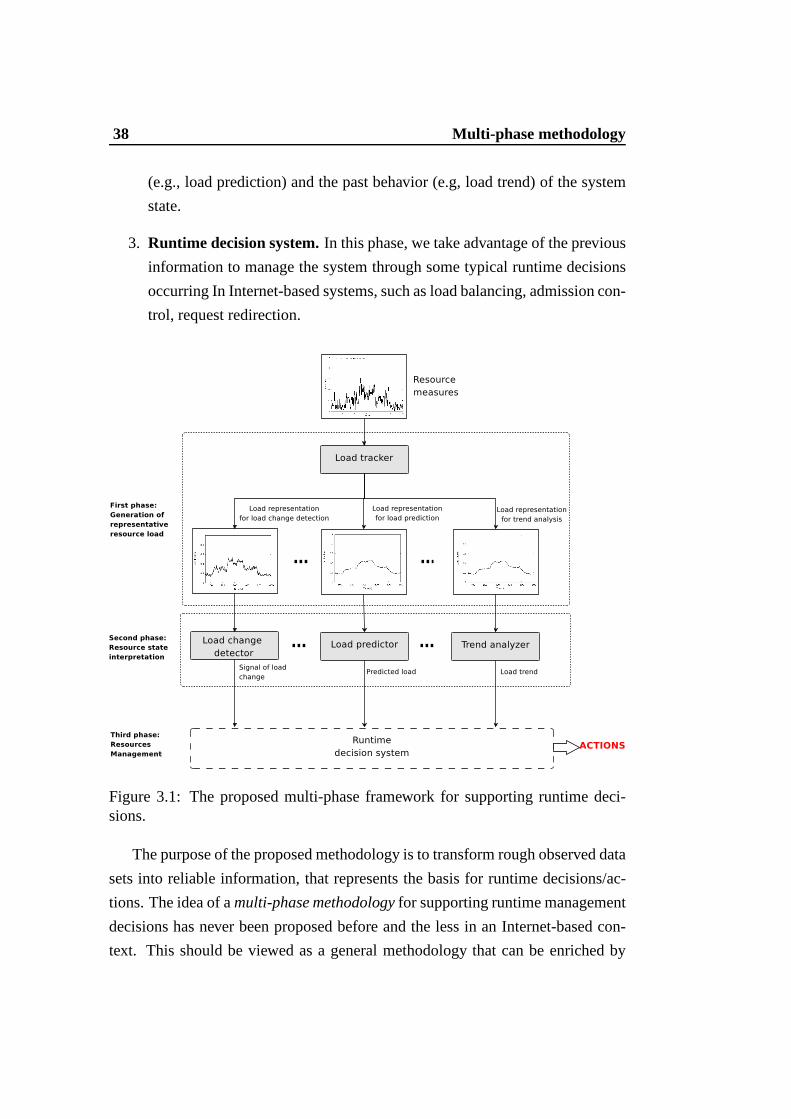
38 Multi-phase methodology
(e.g., load prediction) and the past behavior (e.g, load trend) of the system
state.
3. Runtime decision system.In this phase, we take advantage of the previous
information to manage the system through some typical runtime decisions
occurring In Internet-based systems, such as load balancing, admission con-
trol, request redirection.
Figure 3.1: The proposed multi-phase framework for supporting runtime deci-sions.
The purpose of the proposed methodology is to transform rough observed data
sets into reliable information, that represents the basis for runtime decisions/ac-
tions. The idea of amulti-phase methodologyfor supporting runtime management
decisions has never been proposed before and the less in an Internet-based con-
text. This should be viewed as a general methodology that canbe enriched by
Representative resource load 39
other models and decision support systems. This idea opens several interesting
issues that we will address in the following chapters.
3.1.1 Representative resource load
In the proposedmulti-phase methodology, the generation of a representative re-
source load is the fundamental step for supportingadaptiveandself-adaptiveac-
tivities. Its main task is to transform the unusable observed data set into reliable
information.
The first-phase of our methodology takes the observed data and produces load
representations through stochastic models based on filtering and smoothing func-
tions that we callload trackers. They get continuously measures from the system
monitors and evaluate an adequate load representation of the internal resource
behavior for each class of application (e.g load change detectors, predictors) as
described in Figure 3.1.
The transformation from rough data into useful informationis based on the
estimation theorythat assumes that the observed data set is embedded into a noisy
signal. Numerous fields require the use of estimation theory: interpretation of
scientific experiments, signal processing, quality control, telecommunications,
control theory. We apply this theory to Internet-based systems. Two important
components of theestimation theoryare thefiltering andsmoothingtheories that
propose many techniques to reduce the noise component such as the Kalman filter,
the low-pass filters, the moving averages, linear and non linear regression func-
tions.
The choice of an adequate load tracker is of utmost importance to the entire
runtime management system. We propose load trackers based on linear and non-
linear models with different choices of parameters.
3.1.2 Resource state interpretation
In the second phase of the methodology, each system representation obtained
through the load trackers is passed to an evaluation module that should inter-
pret the resource state. The goal is to evaluate the information that is provided
by the load trackers and to communicate the results to theruntime decision sys-

40 Multi-phase methodology
tem. For this second phase, we consider three main classes of state interpretation
algorithms that have to solve classical problems, such as detecting non-transient
changes of the load conditions of a system resource, predicting the future resource
state, and defining the resource behavioral trend.
In Figure 3.1 we show that different resource state interpretation algorithms
may require different representations that can be generated by the load tracker.
For example, a valid load change detector should signal to the runtime decision
system only significant load changes that require some immediate actions, such
as redirecting requests and filtering accesses. On the otherhand, a load predictor
should provide the runtime decision system with expected future load conditions
that are at the basis of different algorithms, such as load balancing and request
dispatching.
• Load change detection. Many runtime decision systems related to the
Internet-based context are activated after a significant load variation has
occurred in some system resources. Request redirection, process migration,
access control and limitation are some examples of processes that are ac-
tivated after the detection of a significant and non-transient load change.
Different load change detection algorithms exist and they are characterized
by different characteristics (for example, runtime vs. off-line detection), but
all of them share the common trait to require a reliable representation of the
resource load.
• Load prediction. The ability of forecasting the future load from a set of
past values is another key function for many runtime decision systems that
manage Internet-based services. There are a plethora of prediction models
that aim to support time series forecasting: linear time series, neural net-
works, wavelet analysis, support vector machines (SVM), fuzzy systems.
The choice of the most appropriate prediction model dependson the re-
quirements of the application context. Most of the prediction models are
designed for off-line applications. As we are interested toruntime predic-
tion models, genetic algorithms, neural networks, SVM, fuzzy systems are
inadequate because they achieve a valid accuracy at the price of unaccept-
able computational costs for prediction and learning time.
Runtime decision systems 41
• Load trend analysis. For many runtime decision systems, it is important
not only to know the present load state and predict the futureload condi-
tions, but also to understand from where the system is coming. This is the
goal of the analysis that we applied to different decision algorithms.
3.1.3 Runtime decision systems
The majority of Internet-based services is supported by complex distributed in-
frastructures that have to satisfy scalability and availability requirements, and have
to avoid performance degradation and system overload. Managing these systems
requires a large set of runtime decision algorithms that areoriented to load balanc-
ing, load sharing, overload and admission control, job dispatching and redirection
even at a geographical scale.
The runtime decision systems can be classified in two main classes that we
call: decision systemsandautonomic decision systems. The first class is charac-
terized by systems composed by highly coupled components and require reliable
information about the global system state. The system is managed thanks to some
centralized algorithms that take decision on the basis of the information about
all the monitored components. The second class regards the autonomic environ-
ment that is typically characterized by loosely coupled components, by few or null
global information about the state of their components and by distributed manage-
ment algorithms. In this thesis, we will apply the proposed methodology to both
classes of runtime decision systems.
3.2 Internet-based systems
In this section, we describe the characteristics of a representative example of an
Internet-based system that consists of a popular multi-tier Web architecture for the
generation of dynamic contents. This test-bed system will be exercised through
a large set of synthetic and realistic workload models. These experiments will
generate several data sets referring to the system resourcemeasures. We use these
data sets to evaluate the properties of stochastic models for load representation,
load change detection, load prediction and load trend analysis. This section is

42 Multi-phase methodology
divided in three parts:
• description of the test-bed system;
• presentation of the synthetic and realistic workload models that will be used
in large parts of the thesis;
• description of the most important resource measures that will represent the
basic data sets for several analyses throughout the thesis.
3.2.1 Case study: test-bed system
The typical infrastructure for supporting Web-based services is based on a multi-
tier logical architecture that tends to separate the three main functions of service
delivery: the HTTP interface, the application (or business) logic and the informa-
tion repository.
These logical architecture layers are referred to as the front-end, application,
and back-end layers, are shown in Figure 3.2.
Figure 3.2: Typical architecture of a Web-based system
The front-end layer is the interface of the Web-based service. It accepts HTTP
connection requests from the clients, serves static content from the file system,
and represents an interface towards the application logic of the middle layer. The
most popular software for implementing the front-end layeris the Apache Web
server [4]. The application layer is at the heart of a Web-based service: it handles
all the business logic and retrieves the information which is used to build responses
with dynamically generated content. This last step often requires interactions with
the back-end layer, hence the application layer must be capable of interfacing
Workload models 43
the application logic with the data storage at the back-end.The back-end layer
manages the main information repository of a Web-based service. It typically
consists of a database server and storage of critical information that is the main
source for generating dynamic content.
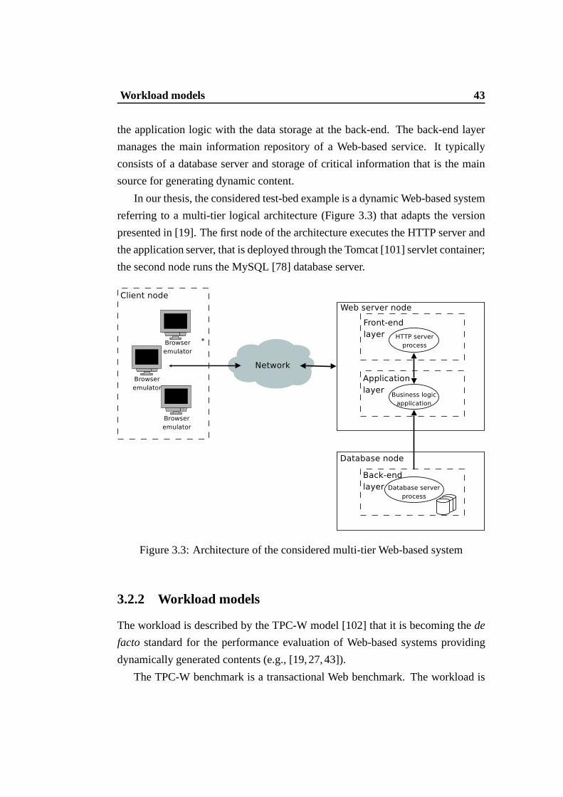
In our thesis, the considered test-bed example is a dynamic Web-based system
referring to a multi-tier logical architecture (Figure 3.3) that adapts the version
presented in [19]. The first node of the architecture executes the HTTP server and
the application server, that is deployed through the Tomcat[101] servlet container;
the second node runs the MySQL [78] database server.
Figure 3.3: Architecture of the considered multi-tier Web-based system
3.2.2 Workload models
The workload is described by the TPC-W model [102] that it is becoming thede
facto standard for the performance evaluation of Web-based systems providing
dynamically generated contents (e.g., [19,27,43]).
The TPC-W benchmark is a transactional Web benchmark. The workload is
44 Multi-phase methodology
exercised in a controlled Internet commerce environment that simulates the activ-
ities of a business oriented transactional Web server. The workload exercises a
breadth of system components, which are characterized by:
• multiple on-line browser sessions;
• dynamic page generation with database access and update;
• consistent Web objects;
• simultaneous execution of multiple transaction types that span a breadth of
complexity;
• on-line transaction execution modes;
• databases consisting of many tables with a wide variety of sizes, attributes,
and relationships;
• transaction integrity;
• contention on data access and update.
The performance metric reported by TPC-W is the number of Webinteractions
processed per second. Multiple Web interactions are used tosimulate the activ-
ity of a retail store, and each interaction is subject to a response time constraint.
TPC-W simulates three different profiles by varying the ratio of browse to buy:
primarily shopping, browsing and Web-based ordering. Client requests are gener-
ated through a set ofemulated browsers, where each browser is implemented as a
Java thread reproducing an entire User Session with the Web site.
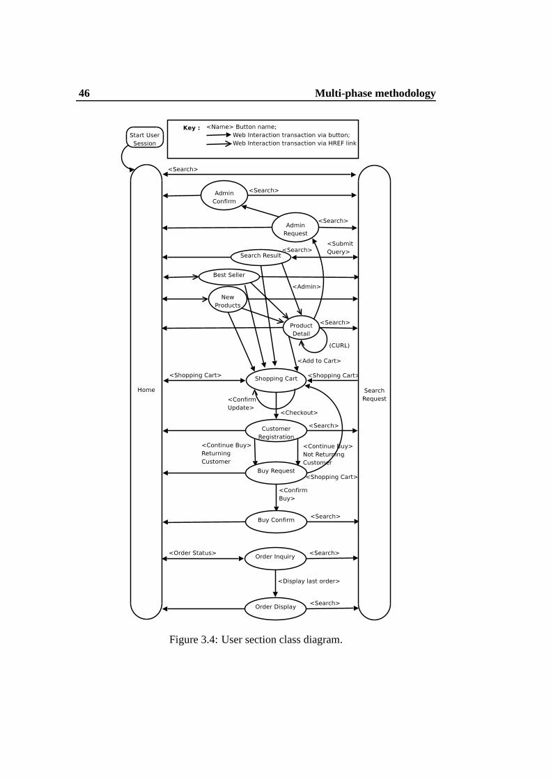
The diagram of Figure 3.4 shows the sequences of the Web interactions. Dur-
ing a User Session each Emulated Browser generates a sequence of Web inter-
actions that correspond to a traversal of this diagram. Eachnode in the diagram
contains the name of a Web interaction type (Home, Best Seller, Search Request,
etc.). An arrow between two nodes A and B indicates that afterperforming Web
interaction A, it is possible for an Emulated Browser to nextperform the Web in-
teraction B. When there are multiple arrows leaving a node, the arc that is chosen
for the Web interaction is determined probabilistically asdescribed in Table 3.1.
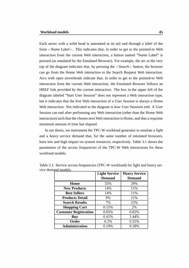
Workload models 45
Each arrow with a solid head is annotated at its tail end through a label of the
form <Name Label>. This indicates that, in order to get to the pointed-to Web
interaction from the current Web interaction, a button named ”Name Label” is
pressed (as emulated by the Emulated Browser). For example,the arc at the very
top of the diagram indicates that, by pressing the<Search> button, the browser
can go from the Home Web interaction to the Search Request Webinteraction.
Arcs with open arrowheads indicate that, in order to get to the pointed-to Web
interaction from the current Web interaction, the EmulatedBrowser follows an
HREF link provided by the current interaction. The box in theupper left of the
diagram labeled ”Start User Session” does not represent a Web interaction type,
but it indicates that the first Web interaction of a User Session is always a Home
Web interaction. Not indicated in the diagram is how User Sessions end. A User
Session can end after performing any Web interaction (otherthan the Home Web
interaction) such that the chosen next Web interaction is Home, and that a requisite
minimum amount of time has elapsed.
In our thesis, we instrument the TPC-W workload generator toemulate alight
and aheavyservice demand that, for the same number of emulated browsers,
have low and high impact on system resources, respectively.Table 3.1 shows the
parameters of the access frequencies of the TPC-W Web interactions for these
workload models.
Table 3.1: Service access frequencies (TPC-W workload) forlight and heavy ser-vice demand models.
Light Service Heavy ServiceDemand Demand
Home 55% 29%New Products 14% 11%Best Sellers 14% 11%
Products Detail 9% 21%Search Results 7% 23%Shopping Cart 0.15% 2%
Customer Registration 0.05% 0.82%Buy 0.41% 1.44%
Order 0.2% 0.55%Administration 0.19% 0.18%
46 Multi-phase methodology
Figure 3.4: User section class diagram.

Workload models 47
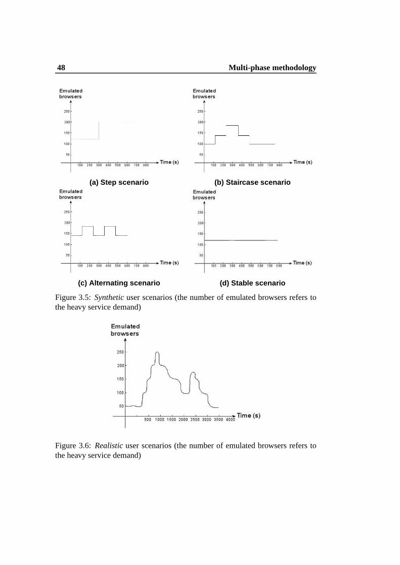
For both service demand models, fiveuser scenariosare implemented by vary-
ing the number of emulated browsers over time. The data sets generated by these
workloads are used for all successive analysis of themulti-phase methodology
because they are considered representative workload models of a typical Internet-
based system. Some representative synthetic user scenarios referring to the heavy
workload model are shown in Figure 3.5. (Analogous patternswith different num-
bers of emulated browsers are created for the light service demand model.)
• Step scenario.The scenario in Figure 3.5 (a) describes a sudden load in-
crement from a relatively unloaded to a more loaded system [91]. The pop-
ulation is kept at 120 emulated browsers for 5 minutes, then it is suddenly
increased to 200 emulated browsers for other 5 minutes.
• Staircase scenario. The scenario in Figure 3.5 (b) represents a gradual
increment of the population up to 180 emulated browsers thatis followed
by a similar gradual decrease.
• Alternating scenario. The scenario in Figure 3.5 (c) describes an alter-
nating increase and decrease of the load between 140 and 180 emulated
browsers every two minutes.
• Stable scenario.The scenario in Figure 3.5 (d) describes an ideal workload
where the number of emulated browsers does not change duringthe exper-
iment. The population refers to 120 emulated browsers issuing requests for
800 seconds. We should observe that a stable number of clients does not
means that the requests reaching the Internet-based systems are always the
same.
• Realistic scenario. The scenario in Figure 3.6 reproduces a realistic user
pattern (e.g., [10]) where load changes are characterized by a continuous
and gradual increase or decrease of the number of emulated browsers.
These ten workload models are representative of the typicalWeb workload that
is characterized by heavy-tailed distributions [5,8,28,38] and by flash crowds [59]
that contribute to augment the skew of raw data.
48 Multi-phase methodology
(a) Step scenario (b) Staircase scenario
(c) Alternating scenario (d) Stable scenario
Figure 3.5:Syntheticuser scenarios (the number of emulated browsers refers tothe heavy service demand)
Figure 3.6:Realisticuser scenarios (the number of emulated browsers refers tothe heavy service demand)
Resource measures 49
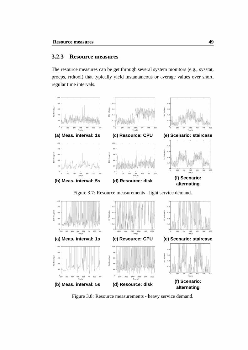
3.2.3 Resource measures
The resource measures can be get through several system monitors (e.g., sysstat,
procps, rrdtool) that typically yield instantaneous or average values over short,
regular time intervals.
0
200
400
600
800
1000
0 100 200 300 400 500 600
Dis
k th
roug
hput
Time [s]
(a) Meas. interval: 1s
0
0.2
0.4
0.6
0.8
1
0 100 200 300 400 500 600
CP
U u
tiliz
atio
n
Time [s]
(c) Resource: CPU
0
0.2
0.4
0.6
0.8
1
0 100 200 300 400 500 600
CP
U u
tiliz
atio
n
Time [s]
(e) Scenario: staircase
0
200
400
600
800
1000
0 100 200 300 400 500 600
Dis
k th
roug
hput
Time [s]
(b) Meas. interval: 5s
0
200
400
600
800
1000
0 100 200 300 400 500 600
Dis
k th
roug
hput
Time [s]
(d) Resource: disk
0
0.2
0.4
0.6
0.8
1
0 100 200 300 400 500 600
CP
U u
tiliz
atio
n
Time [s]
(f) Scenario:alternating
Figure 3.7: Resource measurements - light service demand.
0
200
400
600
800
1000
200 300 400 500 600 700 800 900
Dis
k th
roug
hput
Time [s]
(a) Meas. interval: 1s
0
0.2
0.4
0.6
0.8
1
1500 1600 1700 1800 1900 2000
CP
U U
tiliz
atio
n
Time [s]
(c) Resource: CPU
0
0.2
0.4
0.6
0.8
1
0 100 200 300 400 500 600
CP
U U
tiliz
atio
n
Time [s]
(e) Scenario: staircase
0
200
400
600
800
1000
200 300 400 500 600 700 800 900
Dis
k th
roug
hput
Time [s]
(b) Meas. interval: 5s
0
200
400
600
800
1000
1500 1600 1700 1800 1900 2000
Dis
k th
roug
hput
Time [s]
(d) Resource: disk
0
0.2
0.4
0.6
0.8
1
0 100 200 300 400 500 600
CP
U U
tiliz
atio
n
Time [s]
(f) Scenario:alternating
Figure 3.8: Resource measurements - heavy service demand.

50 Multi-phase methodology
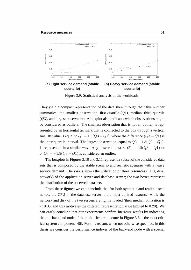
In order to have a qualitative representation of the behavior of commonly mea-
sured resources (CPU utilization, disk and network throughput (MB/sec)), in Fig-
ures 3.7 and 3.8 we report the measures related to the light and heavy scenario,
respectively, for different sample periods and workload classes by considering:
• two resource measurement intervals: 1 second (Figures 3.7(a) and 3.8 (a)),
and 5 seconds (Figures 3.7 (b) and 3.8 (b));
• two resource metrics: CPU utilization (Figures 3.7 (c) and3.8 (c)), and disk
throughput as blocks/second (Figures 3.7 (d) and 3.8 (d));
• four user scenarios: step (Figures 3.7 (c), 3.7 (d), 3.8 (c)and 3.8 (d))),
staircase (Figures 3.7 (e) and 3.8 (e)), realistic (Figures3.7 (a), 3.7 (b), 3.8
(a) and 3.8 (b))), alternating (Figures 3.7 (f) and 3.8 (f)).
All these figures share the common trait that the resource measures, obtained
from system monitors are extremely variable to the extent that any runtime de-
cision based on these values may be risky when not completelywrong. If we
compare the two workload classes, the Figures 3.7 and 3.8 show that the heavy
service demand causes a much higher variability of the resource measures than
that obtained by the light service demand. We give a mathematical confirmation
of this observation by evaluating the mean and the standard deviation of the CPU
utilization of the back-end node for both workload classes.We consider six stable
user scenarios where the number of emulated browsers is keptfixed during the
experiment running for one hour. The initial and last ten minutes are considered
as warm-up and cool-down periods, hence they are omitted from the evaluation of
the statistics. The average CPU utilization and its standard deviation for the light
and heavy workload are shown in Figures 3.9 (a) and 3.9 (b), respectively. These
results confirm the high variability of the resource measures for both workloads.
In particular, the standard deviation evidences a twofold dispersion of the resource
measures in the case of heavy service demand.
Moreover, it is important to identify the representative internal performance
index of the most critical resource of the considered Internet-based system. To this
purpose, we analyze the performance of the CPU, disk and network of the appli-
cation and database servers and show the results through boxplot diagrams [104].
Resource measures 51
0
0.2
0.4
0.6
0.8
1
200 300 400 500 600 700
CP
U-u
tiliz
atio
n
Emulated Browsers
Standard deviationMean
(a) Light service demand (stablescenario)
0
0.2
0.4
0.6
0.8
1
100 120 140 160 180 200
CP
U u
tiliz
atio
n
Emulated Browsers
Standard deviationMean
(b) Heavy service demand (stablescenario)
Figure 3.9: Statistical analysis of the workloads.
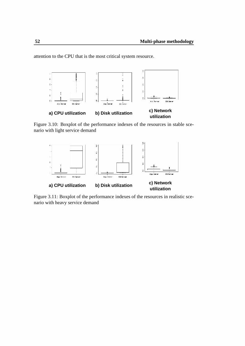
They yield a compact representation of the data skew throughtheir five number
summaries: the smallest observation, first quartile (Q1), median, third quartile
(Q3), and largest observation. A boxplot also indicates which observations might
be considered as outliers. The smallest observation that isnot an outlier, is rep-
resented by an horizontal tic mark that is connected to the box through a vertical
line. Its value is equal toQ1− 1.5(Q3−Q1), where the difference(Q3−Q1) is
the inter-quartile interval. The largest observation, equal toQ3 + 1.5(Q3 − Q1),
is represented in a similar way. Any observed data< Q1 − 1.5(Q3 − Q1) or
> Q3 − +1.5(Q3 − Q1) is considered an outlier.
The boxplots in Figures 3.10 and 3.11 represent a subset of the considered data
sets that is composed by the stable scenario and realistic scenario with a heavy
service demand. The y-axis shows the utilization of three resources (CPU, disk,
network) of the application server and database server; thetwo boxes represent
the distribution of the observed data sets.
From these figures we can conclude that for both synthetic andrealistic sce-
narios, the CPU of the database server is the most utilized resource, while the
network and disk of the two servers are lightly loaded (theirmedian utilization is
< 0.05, and this motivates the different representation scale limited to0.20). We
can easily conclude that our experiments confirm literatureresults by indicating
that the back-end node of the multi-tier architecture in Figure 3.3 is the most crit-
ical system component [46]. For this reason, when not otherwise specified, in this
thesis we consider the performance indexes of the back-end node with a special
52 Multi-phase methodology
attention to the CPU that is the most critical system resource.
a) CPU utilization b) Disk utilization c) Networkutilization
Figure 3.10: Boxplot of the performance indexes of the resources in stable sce-nario with light service demand
a) CPU utilization b) Disk utilization c) Networkutilization
Figure 3.11: Boxplot of the performance indexes of the resources in realistic sce-nario with heavy service demand

Chapter 4
Load tracker models
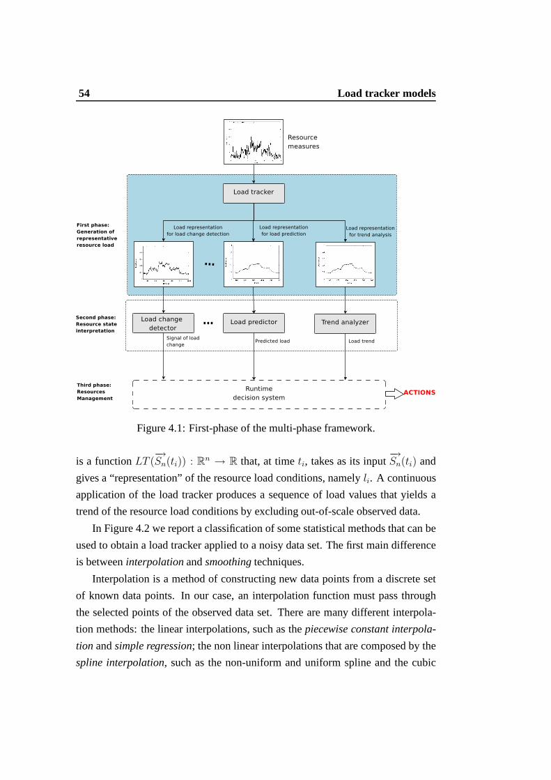
In this chapter, we describe the first phase of themulti-phase methodologyshown
in Figure 4.1. We propose and compare different linear and non-linear functions,
called load trackers, that generateadaptiveandself-adaptiverepresentations of
the resource load and that are suitable to support differentdecision systems and
are characterized by a computational complexity that is compatible with the tem-
poral constraints of runtime decisions. These functions get continuous resource
measures from the system monitors, evaluate a load representation of one or mul-
tiple resources, and pass this representation to the functions of the second phase.
4.1 Definitions
We consider asload trackera function that filters out the noises characterizing a
sequence of low correlated and highly variable measures andyields to the models
of the second phase a more regular view of the load trend of a resource. This
problem is not related just to smooth observed data sets before acting on them
because an arithmetic mean is greatly smoothed, but it may not be representative
of the real load conditions. Different runtime decision systems need different
representations and we should find the right compromise betweenaccuracyand
responsivenessof a load tracker.
At time ti, the load tracker can consider the last observed datasi, and a set
of previously collectedn − 1 measures, that is,−→Sn(ti) = [si−(n−1), . . . , si−1, si]
where thej-th element,i− n + 1 ≤ j ≤ i, is a pairsj = (vj, tj). Theload tracker
54 Load tracker models
Figure 4.1: First-phase of the multi-phase framework.
is a functionLT (−→Sn(ti)) : R
n → R that, at timeti, takes as its input−→Sn(ti) and
gives a “representation” of the resource load conditions, namelyli. A continuous
application of the load tracker produces a sequence of load values that yields a
trend of the resource load conditions by excluding out-of-scale observed data.
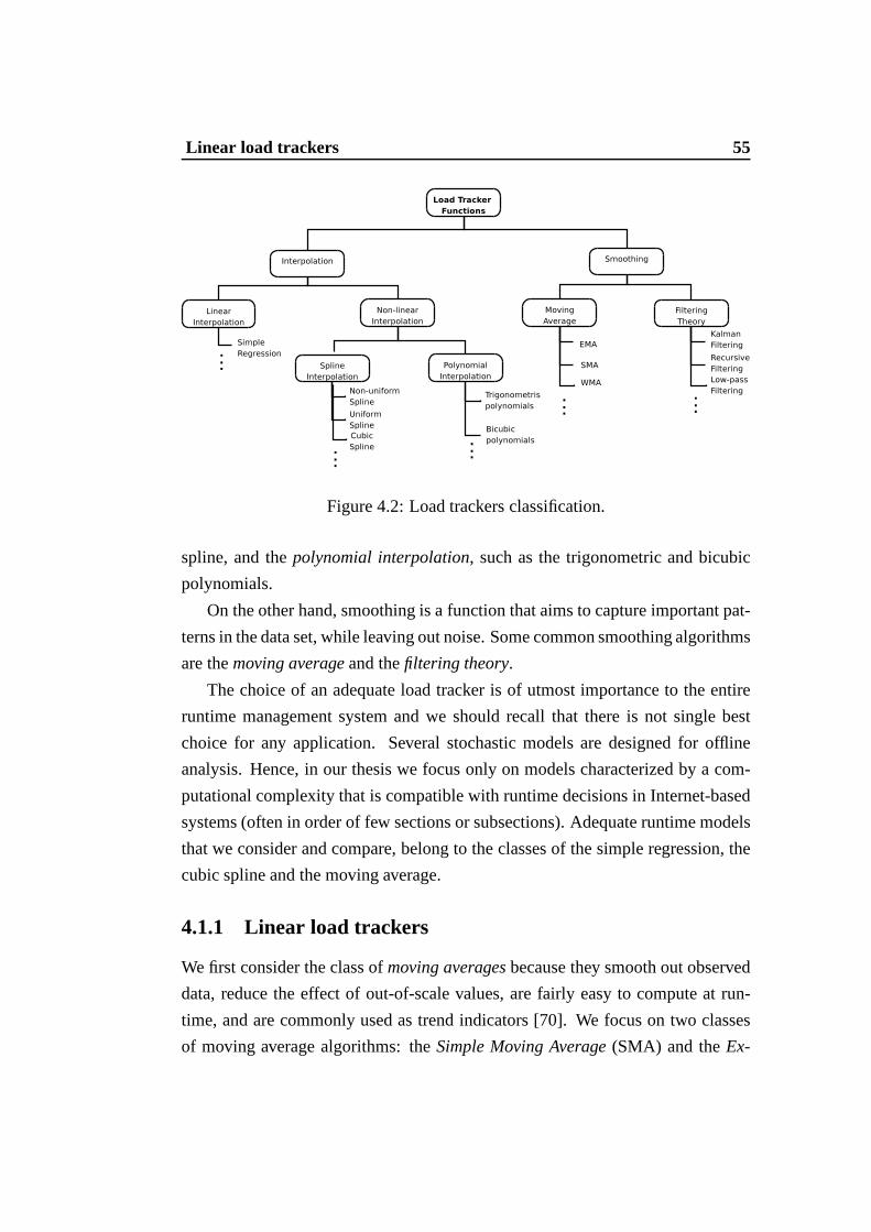
In Figure 4.2 we report a classification of some statistical methods that can be
used to obtain a load tracker applied to a noisy data set. The first main difference
is betweeninterpolationandsmoothingtechniques.
Interpolation is a method of constructing new data points from a discrete set
of known data points. In our case, an interpolation functionmust pass through
the selected points of the observed data set. There are many different interpola-
tion methods: the linear interpolations, such as thepiecewise constant interpola-
tion andsimple regression; the non linear interpolations that are composed by the
spline interpolation, such as the non-uniform and uniform spline and the cubic
Linear load trackers 55
Figure 4.2: Load trackers classification.
spline, and thepolynomial interpolation, such as the trigonometric and bicubic
polynomials.
On the other hand, smoothing is a function that aims to capture important pat-
terns in the data set, while leaving out noise. Some common smoothing algorithms
are themoving averageand thefiltering theory.
The choice of an adequate load tracker is of utmost importance to the entire
runtime management system and we should recall that there isnot single best
choice for any application. Several stochastic models are designed for offline
analysis. Hence, in our thesis we focus only on models characterized by a com-
putational complexity that is compatible with runtime decisions in Internet-based
systems (often in order of few sections or subsections). Adequate runtime models
that we consider and compare, belong to the classes of the simple regression, the
cubic spline and the moving average.
4.1.1 Linear load trackers
We first consider the class ofmoving averagesbecause they smooth out observed
data, reduce the effect of out-of-scale values, are fairly easy to compute at run-
time, and are commonly used as trend indicators [70]. We focus on two classes
of moving average algorithms: theSimple Moving Average(SMA) and theEx-

56 Load tracker models
ponential Moving Average(EMA) that use uniform and non-uniform weighted
distributions of the past measures, respectively. We also consider other popular
linear auto-regressive models [42, 103]:Auto Regressive(AR) andAuto Regres-
sive Integrated Mooving Average(ARIMA).
Simple Moving Average(SMA). It is the unweighted mean of then observed
data values of the vector−→Sn(ti), that is evaluated at timeti (i > n), that is,
SMA(−→Sn(ti)) =
∑
i−(n−1)≤j≤i
sj
n(4.1)
An SMA-based load tracker evaluates a newSMA(−→Sn(ti)) for each measure
si during the observation period. The number of considered observed data values
is a parameter of the SMA model, hence hereafter we use SMAn to denote an
SMA load tracker based onn measures. As SMA models assign an equal weight
to every observed data value, they tend to introduce a significant delay in the trend
representation, especially when the size of the set−→Sn(ti) increases. The EMA
models are often considered with the purpose of limiting this delay effect.
Exponential Moving Average (EMA). It is the weighted mean of then ob-
served data values of the vector−→Sn(ti), where the weights decrease exponentially.
An EMA-based load trackerLT (−→Sn(ti)), at timeti, is equal to:
EMA(−→Sn(ti)) = α ∗ si + (1 − α) ∗ EMA(
−→Sn(ti−1)) (4.2)
where the parameterα = 2/(n+1) is thesmoothing factor. The initialEMA(−→Sn(tn))
value is initialized to the arithmetic mean of the firstn measures:
EMA(−→Sn(tn)) =
∑
0≤j≤n
sj
n(4.3)
Similarly to the SMA model, the number of considered observed data values is
a parameter of the EMA model, hence by EMAn we denote an EMA load tracker
based onn measures.
Auto-Regressive Model(AR). It is a weighted linear combination of the past
p observed data values of the vector−→Sn(ti). An AR-based load tracker at timeti,
Non-linear load trackers 57
can be written as:
AR(−→Sn(ti)) = φ1 ∗ sti + · · · + φp ∗ sti−1−p
+ et (4.4)
whereet ∼ WN(0, σ2) is an independent and identically distributed sequence
(calledresiduals sequence), stn , . . . , stn−1−pare the resources weighted byp lin-
ear coefficients,φ1, . . . , φp are the firstp values of the auto-correlation function
computed on the−→Sn(ti) vector. Thep order of the AR process is determined by
the lag at which the partial auto-correlation function becomes negligible [16, 65].
The numberp of considered observed data values is a parameter of the AR model,
hence by AR(p) we denote an AR load tracker based onp values. Higher-order
auto-regressive models include more laggedsti terms, where the coefficients are
computed on a temporal window of then observed data values.
Auto-Regressive Integrated Moving Average Model(ARIMA). An ARIMA
model is obtained by differentiatingd times a non stationary sequence and by
fitting an ARMA model that is composed by the auto-regressivemodel (AR(p))
and the moving average model (MA(q)). The moving average part is a linear
combination of the pastq noise terms,eti , . . . , eti−1−q[16,65]. An ARIMA model
can be written as:
ARIMA(−→Sn(ti)) = φ1∗sti +· · ·+φp+d∗sti−1−p−d
+θ0∗eti +· · ·+θq∗eti−q(4.5)
whereθ1, . . . , θq are linear coefficients. This model is characterized by three pa-
rameters, that is, ARIMA(p,d,q), wherep is the number of the considered values
of the data set,q is the number of the residuals values, andd is the number of the
differentiating values. As an ARIMA model requires frequent updates of its pa-
rameters, it may require a non-deterministic amount of timeto fit the load tracker
values [42]. Hence, an ARIMA load tracker seems rather inadequate to support
a runtime management system when the underlying infrastructure is subject to
highly variable workloads.
4.1.2 Non-linear load trackers
The linear models tend to introduce a delay in the load trend description when
the size of the considered observed data values increases, while they oscillate too
58 Load tracker models
much when the set is small. The need to consider non-linear trackers is motivated
by the goal of addressing in an alternative way the trade-offthat characterizes
linear models. We consider two non-linear models.
Two sided quartile-weighted median(QWM). In descriptive statistics, the
quantile is a common way of estimating the proportions of thedata that should
fall above and below a given value. The two sided quartile-weighted median is
considered a robust statistic that is independent of any assumption on the distri-
bution of the observed data values [45]. The idea is to estimate the center of the
distribution of a set of measures through the two sided quartile-weighted median:
QWM(−→Sn(tn)) =
Q.75(−→Sn(tn)) + 2 ∗ Q.5(
−→Sn(tn)) + Q.25(
−→Sn(tn))
4(4.6)
whereQp denotes thepth quantile of the−→Sn(tn).
Cubic Spline (CS). A preliminary analysis induces us to consider thecubic
spline function [85], in the version proposed by Forsytheet al. [51], as another
interesting example of non-linear load tracker. This choice is also motivated by
the observation that lower order spline curves (that is, with a degree less than 3)
do not react quickly enough to load changes, while spline curves with a degree
higher than 3 are considered unnecessarily complex, introduce undesired ripples
and are computationally too expensive to be applied in a runtime context. For the
definition of the cubic spline function, let us choose somecontrol points(tj, sj) in
the set of measured load values, wheretj is the measurement time of the measure
sj. A cubic spline functionCSJ(t), based onJ control points, is a set ofJ − 1
piecewise third-order polynomialspj(t), wherej ∈ [1, J − 1], that satisfy the
following properties.
Property 1.The control points are connected through third-order polynomials:{
CSJ(tj) = sj j = 1, . . . , J
CSJ(t) = pj(t) tj < t < tj+1, j = 1, . . . , J − 1(4.7)
Property 2.To guarantee aC2 behavior at each control point the first and second
order derivatives ofpj(t) andpj+1(t) are set equal at timetj , ∀j ∈ {1, . . . , J −2}:{
dpj(tj+1)
dt=
dpj+1(tj+1)
dt,
d2pj(tj+1)
dt2=
d2pj+1(tj+1)
dt2
(4.8)

4.2 Evaluation methods for load trackers 59
If we combine Properties 1 and 2, we obtain the following definition for
CSJ(t):
CSJ(t) =zj+1(t − tj)
3 + zj(tj+1 − t)3
6hi
+ (sj+1
hi
−hj
6zj+1)(t − tj) + (
sj
hj
−hj
6zj)(tj+1 − t)
∀j ∈ {1, . . . , J − 1}
(4.9)
wherehi = ti+1 − ti, andsj are the measured values. Thezj coefficients are
solved by the following system of equations:
z0 = 0
hj−1zj−1 + 2(hj−1 + hj)zj + hjzj+1 = 6(sj+1−sj
hj−
sj−sj−1
hj−1)
zn = 0
(4.10)
The spline-based load trackerLT (−→Sn(ti)), at timeti, is defined as the cubic
spline functionCSJn (ti), that is obtained through a subset ofJ control points from
the vector ofn load measures.
Although the cubic spline load tracker has two parameters and is computa-
tionally more expensive than the SMA and EMA load trackers, it is commonly
used in approximation and smoothing contexts [47,85,110].The cubic spline has
the advantage of being reactive to load changes and it is independent of resource
metrics and workload characteristics. Its computational complexity is compatible
to runtime decision systems, especially if we choose a smallnumber of control
pointsJ . This reason leads us to prefer the lowest number, that is,J = 3.
4.2 Evaluation methods for load trackers
The load trackers should be evaluated in terms of feasibility and quality. We can
consider acceptable only the load trackers that have a computational complexity
which is compatible with runtime requirements. Moreover, it is important to eval-
uate the load trackeraccuracyand responsiveness. We will see that these two
properties are in conflict, hence the perfect load tracker that is characterized by
optimal accuracy and responsiveness does not exist. We anticipate that this trade-
off can be solved by considering the goals of the load trackerapplication. For

60 Load tracker models
example, a runtime decision system that must take immediateactions may prefer
a highly reactive load tracker at the price of some inaccuracy. On the other hand,
when an action has to be carefully evaluated, a decision system may prefer an
accurate load tracker even if it is less reactive.
4.2.1 Computational cost
In this section, we estimate the computational cost of the load tracker functions
to understand their feasibility to runtime requirements. We evaluate the CPU time
required by each load tracker to compute a new value of the load representation.
This time does not include the system and communication times that are neces-
sary to fill the observed data set. The results for different measured values (n) are
evaluated on an average PC machine and reported in Table 4.1.They refer to the
realistic user scenario and heavy service demand, but theircosts are representative
of any workload. From this table we can conclude that the computational cost of
all considered load tracker functions is compatible with runtime constraints. The
majority of load trackers have a CPU time well below 10 msec. The main differ-
ence is represented by the ARIMA models with a computationalcost that is one
order of magnitude higher. Although a cost below 100msec. seems compatible
with many runtime decision systems, we should consider thatbehind the choice
of the parameters of the AR and ARIMA models there is a complexevaluation of
the auto-correlation and partial auto-correlation functions as in [16, 65]. For ex-
ample, we can conclude that the AR(32) and ARIMA(1,0,1) models are the best
parameters for the considered workload. The complexity of this phase, rather than
the CPU time for generating a load tracker value, leads us to consider that the AR
and ARIMA models are inadequate to support runtime decisionsystems in highly
variable workload scenarios.
4.2.2 Accuracy and responsiveness
All the considered load trackers share the common goal of representing at runtime
the trend of a set of observed values obtained from some load monitor. For the
evaluation of the load tracker accuracy and responsiveness, we need a reference
curve that we callrepresentative load interval. This is the indicator of the central
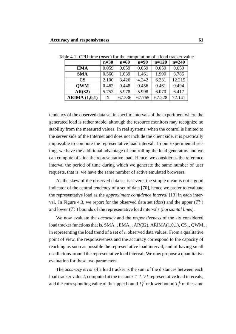
Accuracy and responsiveness 61
Table 4.1: CPU time (msec) for the computation of a load tracker valuen=30 n=60 n=90 n=120 n=240
EMA 0.059 0.059 0.059 0.059 0.059SMA 0.560 1.039 1.461 1.990 3.785CS 2.100 3.426 4.242 6.231 12.215
QWM 0.462 0.448 0.456 0.461 0.494AR(32) 5.752 5.978 5.998 6.070 6.417
ARIMA (1,0,1) X 67.536 67.765 67.228 72.141
tendency of the observed data set in specific intervals of theexperiment where the
generated load is rather stable, although the resource monitors may recognize no
stability from the measured values. In real systems, when the control is limited to
the server side of the Internet and does not include the client side, it is practically
impossible to compute the representative load interval. Inour experimental set-
ting, we have the additional advantage of controlling the load generators and we
can compute off-line the representative load. Hence, we consider as the reference
interval the period of time during which we generate the samenumber of user
requests, that is, we have the same number of active emulatedbrowsers.
As the skew of the observed data set is severe, the simple meanis not a good
indicator of the central tendency of a set of data [70], hencewe prefer to evaluate
the representative load as theapproximate confidence interval[13] in each inter-
val. In Figure 4.3, we report for the observed data set (dots) and the upper (T UI )
and lower (T LI ) bounds of the representative load intervals (horizontal lines).
We now evaluate theaccuracyand theresponsivenessof the six considered
load tracker functions that is, SMAn, EMAn, AR(32), ARIMA(1,0,1), CSn, QWMn,
in representing the load trend of a set ofn observed data values. From a qualitative
point of view, the responsiveness and the accuracy correspond to the capacity of
reaching as soon as possible the representative load interval, and of having small
oscillations around the representative load interval. We now propose a quantitative
evaluation for these two parameters.
Theaccuracy errorof a load tracker is the sum of the distances between each
load tracker valueli computed at the instanti ∈ I, ∀I representative load intervals,
and the corresponding value of the upper boundT UI or lower boundT L
I of the same
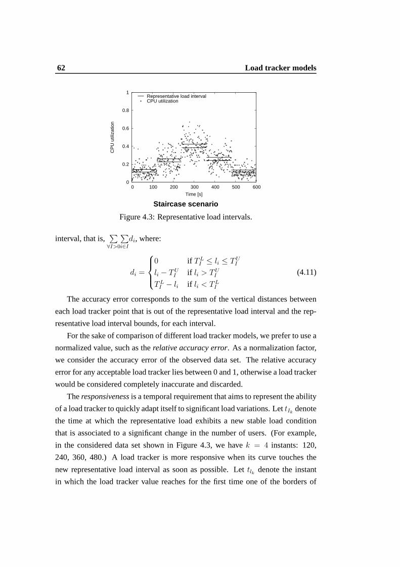
62 Load tracker models
0
0.2
0.4
0.6
0.8
1
0 100 200 300 400 500 600
CP
U u
tiliz
atio
n
Time [s]
Representative load intervalCPU utilization
Staircase scenario
Figure 4.3: Representative load intervals.
interval, that is,∑
∀I>0
∑
i∈I
di, where:
di =
0 if T LI ≤ li ≤ TU
I
li − TUI if li > TU
I
TLI − li if li < TL
I
(4.11)
The accuracy error corresponds to the sum of the vertical distances between
each load tracker point that is out of the representative load interval and the rep-
resentative load interval bounds, for each interval.
For the sake of comparison of different load tracker models,we prefer to use a
normalized value, such as therelative accuracy error. As a normalization factor,
we consider the accuracy error of the observed data set. The relative accuracy
error for any acceptable load tracker lies between 0 and 1, otherwise a load tracker
would be considered completely inaccurate and discarded.
Theresponsivenessis a temporal requirement that aims to represent the ability
of a load tracker to quickly adapt itself to significant load variations. LettIkdenote
the time at which the representative load exhibits a new stable load condition
that is associated to a significant change in the number of users. (For example,
in the considered data set shown in Figure 4.3, we havek = 4 instants: 120,
240, 360, 480.) A load tracker is more responsive when its curve touches the
new representative load interval as soon as possible. Lettlk denote the instant
in which the load tracker value reaches for the first time one of the borders of

4.3 Results 63
the representative load interval that is associated with a new load condition. The
responsiveness errorof a load tracker is measured as the sum of the horizontal
differences between the initial instanttIkcharacterizing the representative loadI
and the corresponding timetlk that is necessary to the load tracker to touch this
new interval. For comparison reasons, we normalize the sum of the time delays
by the total observation periodT , thus obtaining arelative responsiveness error,∑
k
|tIk− tlk |
T(4.12)
We have carried out a very large set of experiments for analyzing the typical
behavior of commonly measured resources. We report a subsetof the results that
refer to a specific architecture for ten classes of workload.The reader should be
aware that the main observations and conclusions about these results are represen-
tative of the typical behavior of the resources of an Internet-based system that is
subject to realistic workload.
4.3 Results
We apply the load tracker analysis of the multi-phase methodology to typical in-
ternal resources measures of an Internet-based system and we evaluate the accu-
racy, responsiveness and precision of six load tracker models. As a representative
example, we consider the workloads and the Internet-based system described in
Section 3.2
4.3.1 Accuracy
The evaluation of the load tracker models requires a preliminary step for the com-
putation of the representative load interval for every considered data set. For ex-
ample, in the step scenario and light service demand, we havetwo reference inter-
vals:T1 = [0, 300] andT2 = [301, 600]. In the staircase and alternating scenarios,
there are five reference intervals: [0, 120], [121, 240], [241, 360], [361, 480] and
[481, 600]. In the realistic scenario, we consider four intervals: [341, 460], [500,
640], [701, 820] and [821, 1000]. In Figures 4.4 and 4.5, we report, for the six
workloads, the observed data set (dots) and the upper (T UI ) and lower (T L
I ) bounds
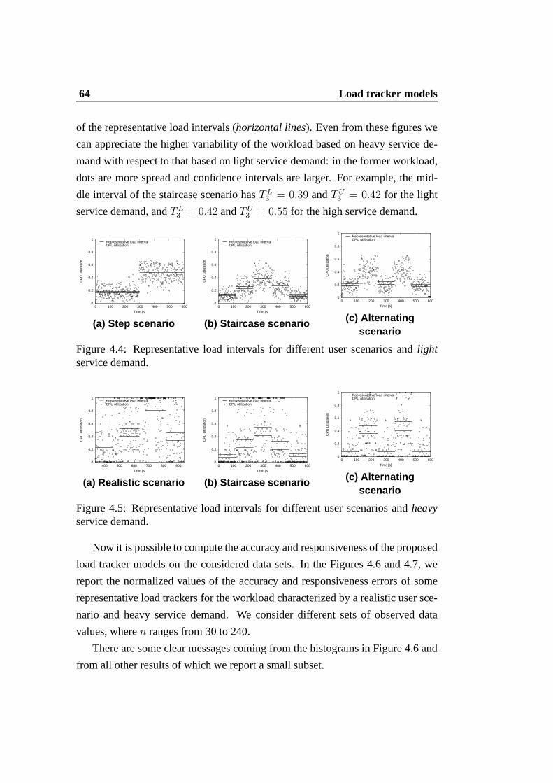
64 Load tracker models
of the representative load intervals (horizontal lines). Even from these figures we
can appreciate the higher variability of the workload basedon heavy service de-
mand with respect to that based on light service demand: in the former workload,
dots are more spread and confidence intervals are larger. Forexample, the mid-
dle interval of the staircase scenario hasT L3 = 0.39 andT U
3 = 0.42 for the light
service demand, andT L3 = 0.42 andT U
3 = 0.55 for the high service demand.
0
0.2
0.4
0.6
0.8
1
0 100 200 300 400 500 600
CP
U u
tiliz
atio
n
Time [s]
Representative load intervalCPU utilization
(a) Step scenario
0
0.2
0.4
0.6
0.8
1
0 100 200 300 400 500 600
CP
U u
tiliz
atio
n
Time [s]
Representative load intervalCPU utilization
(b) Staircase scenario
0
0.2
0.4
0.6
0.8
1
0 100 200 300 400 500 600
CP
U u
tiliz
atio
n
Time [s]
Representative load intervalCPU utilization
(c) Alternatingscenario
Figure 4.4: Representative load intervals for different user scenarios andlightservice demand.
0
0.2
0.4
0.6
0.8
1
400 500 600 700 800 900
CP
U U
tiliz
atio
n
Time [s]
Representative load intervalCPU utilization
(a) Realistic scenario
0
0.2
0.4
0.6
0.8
1
0 100 200 300 400 500 600
CP
U U
tiliz
atio
n
Time [s]
Representative load intervalCPU utilization
(b) Staircase scenario
0
0.2
0.4
0.6
0.8
1
0 100 200 300 400 500 600
CP
U U
tiliz
atio
n
Time [s]
Rapresentative load intervalCPU utilization
(c) Alternatingscenario
Figure 4.5: Representative load intervals for different user scenarios andheavyservice demand.
Now it is possible to compute the accuracy and responsiveness of the proposed
load tracker models on the considered data sets. In the Figures 4.6 and 4.7, we
report the normalized values of the accuracy and responsiveness errors of some
representative load trackers for the workload characterized by a realistic user sce-
nario and heavy service demand. We consider different sets of observed data
values, wheren ranges from 30 to 240.
There are some clear messages coming from the histograms in Figure 4.6 and
from all other results of which we report a small subset.
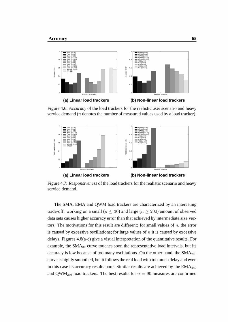
Accuracy 65
0
0.2
0.4
0.6
0.8
1
Realistic scenario
Acc
urac
y er
ror
EMA (n=30)EMA (n=60)EMA (n=90)EMA (n=120)EMA (n=240)SMA (n=30)SMA (n=60)SMA (n=90)SMA (n=120)SMA (n=240)ARIMA (1,0,1)AR (32)
(a) Linear load trackers
0
0.2
0.4
0.6
0.8
1
Realistic scenario
Acc
urac
y er
ror
QWM (n=30)QWM (n=60)QWM (n=90)QWM (n=120)QWM (n=240)CS (n=30)CS (n=60)CS (n=90)CS (n=120)CS (n=240)
(b) Non-linear load trackers
Figure 4.6:Accuracyof the load trackers for the realistic user scenario and heavyservice demand (n denotes the number of measured values used by a load tracker).
0
0.2
0.4
0.6
0.8
1
Realistic scenario
Res
pons
iven
ess
erro
r
EMA (n=30)EMA (n=60)EMA (n=90)EMA (n=120)EMA (n=240)SMA (n=30)SMA (n=60)SMA (n=90)SMA (n=120)SMA (n=240)ARIMA (1,0,1)AR(32)
(a) Linear load trackers
0
0.2
0.4
0.6
0.8
1
Realistic scenario
Res
pons
iven
ess
erro
rQWM (n=30)QWM (n=60)QWM (n=90)QWM (n=120)QWM (n=240)CS (n=30)CS (n=60)CS (n=90)CS (n=120)CS (n=240)
(b) Non-linear load trackers
Figure 4.7:Responsivenessof the load trackers for the realistic scenario and heavyservice demand.
The SMA, EMA and QWM load trackers are characterized by an interesting
trade-off: working on a small (n ≤ 30) and large (n ≥ 200) amount of observed
data sets causes higher accuracy error than that achieved byintermediate size vec-
tors. The motivations for this result are different: for small values ofn, the error
is caused by excessive oscillations; for large values ofn it is caused by excessive
delays. Figures 4.8(a-c) give a visual interpretation of the quantitative results. For
example, the SMA30 curve touches soon the representative load intervals, but its
accuracy is low because of too many oscillations. On the other hand, the SMA240curve is highly smoothed, but it follows the real load with too much delay and even
in this case its accuracy results poor. Similar results are achieved by the EMA240and QWM240 load trackers. The best results forn = 90 measures are confirmed
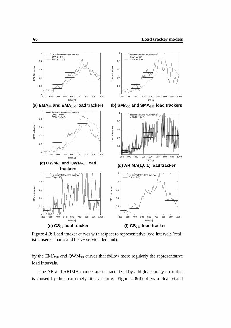
66 Load tracker models
0
0.2
0.4
0.6
0.8
1
200 300 400 500 600 700 800 900 1000
CP
U U
tiliz
atio
n
Time [s]
Representative load intervalEMA (n=90)EMA (n=240)
(a) EMA90 and EMA 240 load trackers
0
0.2
0.4
0.6
0.8
1
200 300 400 500 600 700 800 900 1000
CP
U U
tiliz
atio
n
Time [s]
Representative load intervalSMA (n=30) SMA (n=240)
(b) SMA30 and SMA 240 load trackers
0
0.2
0.4
0.6
0.8
1
200 300 400 500 600 700 800 900 1000
CP
U U
tiliz
atio
n
Time [s]
Representative load intervalQWM (n=90) QWM (n=240)
(c) QWM90 and QWM240 loadtrackers
0
0.2
0.4
0.6
0.8
1
200 300 400 500 600 700 800 900 1000
CP
U U
tiliz
atio
n
Time [s]
Representative load intervalARIMA (1,0,1)
(d) ARIMA(1,0,1) load tracker
0
0.2
0.4
0.6
0.8
1
200 300 400 500 600 700 800 900 1000
CP
U U
tiliz
atio
n
Time [s]
Representative load intervalCS (n=30)
(e) CS30 load tracker
0
0.2
0.4
0.6
0.8
1
200 300 400 500 600 700 800 900 1000
CP
U U
tiliz
atio
n
Time [s]
Representative load intervalCS (n=240)
(f) CS240 load tracker
Figure 4.8: Load tracker curves with respect to representative load intervals (real-istic user scenario and heavy service demand).
by the EMA90 and QWM90 curves that follow more regularly the representative
load intervals.
The AR and ARIMA models are characterized by a high accuracy error that
is caused by their extremely jittery nature. Figure 4.8(d) offers a clear visual
Responsiveness 67
interpretation of the quantitative results. The cubic spline model is quite inter-
esting because larger sets of observed data lead to a monotonic improvement of
the load tracker accuracy. Figures 4.8(e) and 4.8(f) evidence how the curve for
n = 240 follow the representative load interval much better than the cubic spline
for n = 30, that is extremely jittery.
A comparison of all results shows that AR and ARIMA models have the high-
est and unacceptable accuracy errors. The best results of EMA, SMA and QWM
models are comparable and all achieved for a vector ofn = 90 observed values.
Their accuracy is even better than that of the best cubic spline model that is, CS240,
although we will see that this function may have further margins of improvement
for highern.
It is interesting to observe that quite similar results are achieved for completely
different and stressful workloads, such as the step, the staircase and the alternating
user scenarios for both light and heavy service demand. Someresults shown in
Figure 4.9 refer to the light case. They confirm main conclusions about load
tracker models, although they are achieved for different values ofn. In particular,
the SMA, EMA and QWM load trackers obtain their best accuracyfor n = 30
(instead of the previousn = 90 case).
4.3.2 Responsiveness
Let us pass now to evaluate theresponsivenessresults that are reported in the
histograms of Figures 4.7 and 4.10 for the realistic user scenario, and the step, the
staircase and the alternating scenarios, respectively. The message coming from
these figures and from all other results is a clear confirmation of the intuition: for
any load tracker, working on larger data sets increases the responsiveness error.
The most responsive load trackers are the AR and ARIMA modelscharacterized
by a null error. If we exclude these models, that are useless for load tracking
purposes, the cubic spline functions are the most responsive. Even the stability of
their results is appreciable, with an error below 0.1 for anyn < 120. The load
trackers based on the EMA and SMA models seem more sensitive to the choice
of n; acceptable results are obtained forn ≤ 90 and forn ≤ 30 in the light and
heavy service demand case, respectively. The QWM model is typically the less
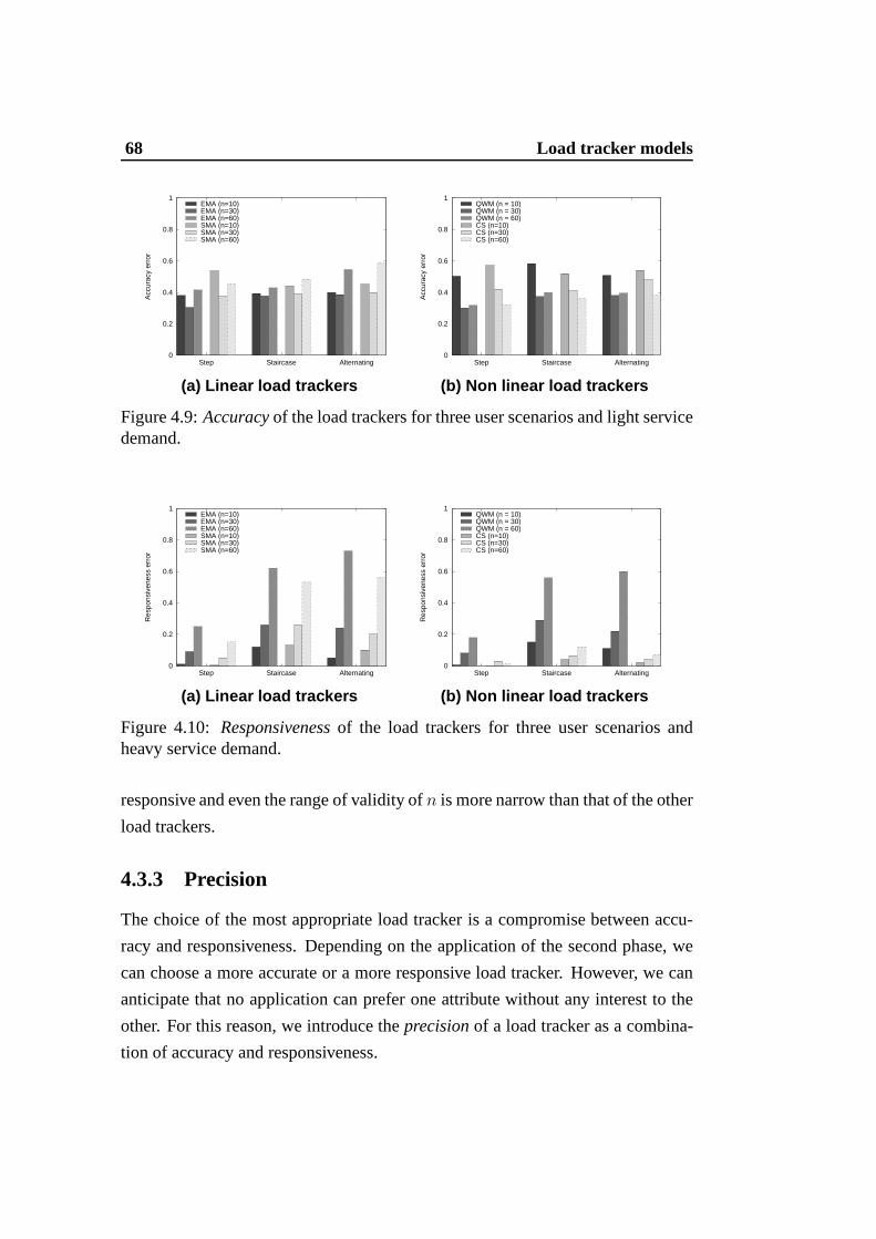
68 Load tracker models
0
0.2
0.4
0.6
0.8
1
AlternatingStaircaseStep
Acc
urac
y er
ror
EMA (n=10)EMA (n=30)EMA (n=60)SMA (n=10)SMA (n=30)SMA (n=60)
(a) Linear load trackers
0
0.2
0.4
0.6
0.8
1
AlternatingStaircaseStep
Acc
urac
y er
ror
QWM (n = 10)QWM (n = 30)QWM (n = 60)CS (n=10)CS (n=30)CS (n=60)
(b) Non linear load trackers
Figure 4.9:Accuracyof the load trackers for three user scenarios and light servicedemand.
0
0.2
0.4
0.6
0.8
1
AlternatingStaircaseStep
Res
pons
iven
ess
erro
r
EMA (n=10)EMA (n=30)EMA (n=60)SMA (n=10)SMA (n=30)SMA (n=60)
(a) Linear load trackers
0
0.2
0.4
0.6
0.8
1
AlternatingStaircaseStep
Res
pons
iven
ess
erro
r
QWM (n = 10)QWM (n = 30)QWM (n = 60)CS (n=10)CS (n=30)CS (n=60)
(b) Non linear load trackers
Figure 4.10: Responsivenessof the load trackers for three user scenarios andheavy service demand.
responsive and even the range of validity ofn is more narrow than that of the other
load trackers.
4.3.3 Precision
The choice of the most appropriate load tracker is a compromise between accu-
racy and responsiveness. Depending on the application of the second phase, we
can choose a more accurate or a more responsive load tracker.However, we can
anticipate that no application can prefer one attribute without any interest to the
other. For this reason, we introduce theprecisionof a load tracker as a combina-
tion of accuracy and responsiveness.
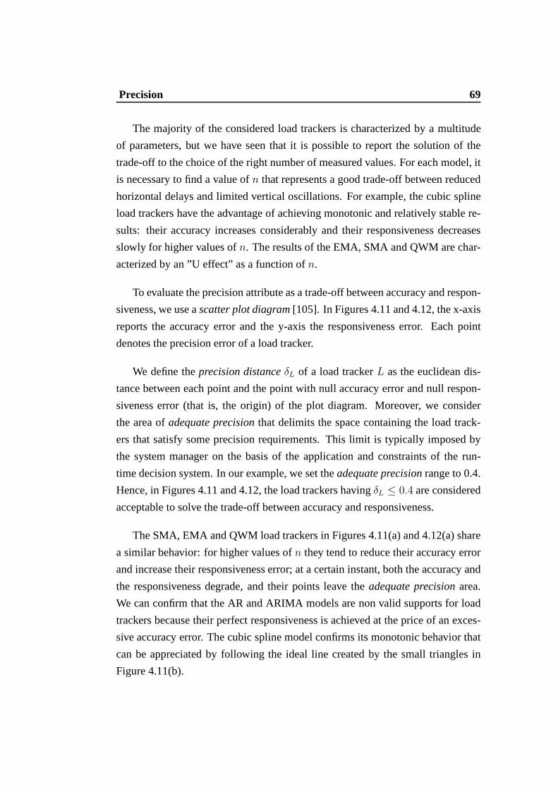
Precision 69
The majority of the considered load trackers is characterized by a multitude
of parameters, but we have seen that it is possible to report the solution of the
trade-off to the choice of the right number of measured values. For each model, it
is necessary to find a value ofn that represents a good trade-off between reduced
horizontal delays and limited vertical oscillations. For example, the cubic spline
load trackers have the advantage of achieving monotonic andrelatively stable re-
sults: their accuracy increases considerably and their responsiveness decreases
slowly for higher values ofn. The results of the EMA, SMA and QWM are char-
acterized by an ”U effect” as a function ofn.
To evaluate the precision attribute as a trade-off between accuracy and respon-
siveness, we use ascatter plot diagram[105]. In Figures 4.11 and 4.12, the x-axis
reports the accuracy error and the y-axis the responsiveness error. Each point
denotes the precision error of a load tracker.
We define theprecision distanceδL of a load trackerL as the euclidean dis-
tance between each point and the point with null accuracy error and null respon-
siveness error (that is, the origin) of the plot diagram. Moreover, we consider
the area ofadequate precisionthat delimits the space containing the load track-
ers that satisfy some precision requirements. This limit istypically imposed by
the system manager on the basis of the application and constraints of the run-
time decision system. In our example, we set theadequate precisionrange to 0.4.
Hence, in Figures 4.11 and 4.12, the load trackers havingδL ≤ 0.4 are considered
acceptable to solve the trade-off between accuracy and responsiveness.
The SMA, EMA and QWM load trackers in Figures 4.11(a) and 4.12(a) share
a similar behavior: for higher values ofn they tend to reduce their accuracy error
and increase their responsiveness error; at a certain instant, both the accuracy and
the responsiveness degrade, and their points leave theadequate precisionarea.
We can confirm that the AR and ARIMA models are non valid supports for load
trackers because their perfect responsiveness is achievedat the price of an exces-
sive accuracy error. The cubic spline model confirms its monotonic behavior that
can be appreciated by following the ideal line created by thesmall triangles in
Figure 4.11(b).
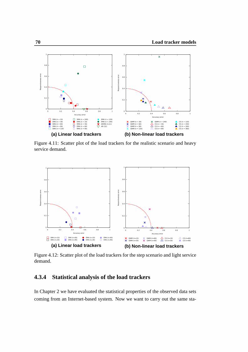
70 Load tracker models
(a) Linear load trackers (b) Non-linear load trackers
Figure 4.11: Scatter plot of the load trackers for the realistic scenario and heavyservice demand.
(a) Linear load trackers (b) Non-linear load trackers
Figure 4.12: Scatter plot of the load trackers for the step scenario and light servicedemand.
4.3.4 Statistical analysis of the load trackers
In Chapter 2 we have evaluated the statistical properties ofthe observed data sets
coming from an Internet-based system. Now we want to carry out the same sta-

4.4 Significance of the results 71
tistical analyses on the load tracker values referring to the same data sets. In
particular we consider the EMA90 load tracker model that has shown “adequate”
precision and evaluate:
• the noise component through the noise indexδ;
• the heteroscedasticity;
• the autocorrelation.
The first interesting result is that the load tracker reducesthe noise indexδ of
about the 80%, passing fromδ = 0.98 for the observed data set toδ = 0.20 for
the load tracker values. We recall thatδ < 0.3 denotes a data set affected by a
significant noise and this bound is clearly satisfied by the load tracker values.
The successive evaluation of the heteroscedasticity of theload tracker values
shows that the variability of the data set variance is greatly reduced to the extent
that it appears similar to a homoscedastic behavior. In Figure 4.13, we compare
the heteroscedasticbehavior of the observed data set that is characterized by a
variable variance of the residuals (Figure 4.13 (a)) and thehomoscedastic-like
behavior of the load tracker values that are characterized by a “constant” variance
of the residuals in the y-axis (Figure 4.13 (b)). The homoscedastic-like behavior
allows the load trackers to respect the same precision quality independently on the
load conditions.
Figure 4.14 shows the ACF functions of the observed data set and the load
tracker values. The load tracker exhibits a slow decay of theauto-correlation
coefficients that bring to a consequent increase of the time dependency between
the values. This property allows us to transform the past values of the load tracker
models in manageable and useful information to represent the present load and to
make prediction.
4.4 Significance of the results
Let us detail the overall significance of the analysis on loadtracker models that
comes from the shown results and other not reported experiments that confirm our
main conclusions.
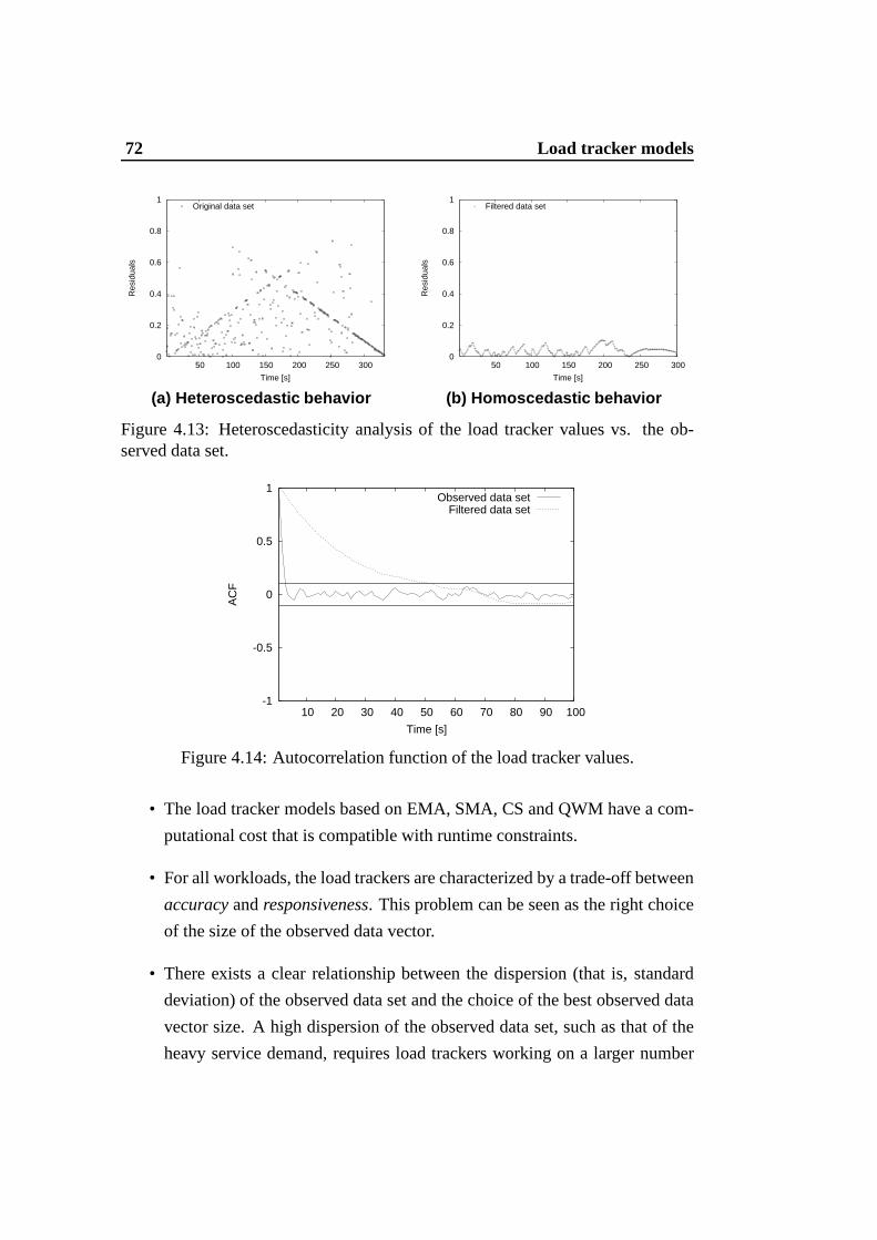
72 Load tracker models
0
0.2
0.4
0.6
0.8
1
50 100 150 200 250 300
Res
idua
ls
Time [s]
Original data set
(a) Heteroscedastic behavior
0
0.2
0.4
0.6
0.8
1
50 100 150 200 250 300
Res
idua
ls
Time [s]
Filtered data set
(b) Homoscedastic behavior
Figure 4.13: Heteroscedasticity analysis of the load tracker values vs. the ob-served data set.
-1
-0.5
0
0.5
1
10 20 30 40 50 60 70 80 90 100
AC
F
Time [s]
Observed data setFiltered data set
Figure 4.14: Autocorrelation function of the load tracker values.
• The load tracker models based on EMA, SMA, CS and QWM have a com-
putational cost that is compatible with runtime constraints.
• For all workloads, the load trackers are characterized by atrade-off between
accuracyandresponsiveness. This problem can be seen as the right choice
of the size of the observed data vector.
• There exists a clear relationship between the dispersion (that is, standard
deviation) of the observed data set and the choice of the bestobserved data
vector size. A high dispersion of the observed data set, suchas that of the
heavy service demand, requires load trackers working on a larger number

4.4 Significance of the results 73
of observed data. On the other hand, the amount of data neededto obtain a
precise load tracker decreases when the workload causes a minor dispersion
of the observed data set.
The proposal of a theoretic methodology to find the “best”n for any load
tracker, any workload and any application is out of the scopeof this thesis. How-
ever, a large set of experimental results points out some interesting empirical evi-
dences.
• There exists a set of feasible values ofn that guarantee an acceptablepreci-
sionof the load tracker.
• The range of feasible values forn depends on the standard deviation of
the observed data set. For example, in the heavy workload case EMA is
acceptable fromn = 30 to n = 120, in the light workload case EMA is
acceptable fromn = 10 to n = 30.
• The QWM-based load tracker has a limited range of feasibility.
• The EMA-based and the SMA-based load trackers have a largerbut still
limited range of feasibility.
• The CS-based load trackers have a sufficientprecisiononly for high values
of n. However, when this load tracker reaches theadequate precisionarea, it
is feasible for a large range ofn values thanks to its monotonic behavior. We
should also consider that its higher accuracy comes at the price of increasing
computational costs, however they do not prevent the application of CS to
runtime contexts.
• Once we are in theadequate precisionarea, all load trackers are feasible.
Among them, we can choose the best load tracker on the basis ofthe require-
ments of the second phase. In other words, we can give more importance
either to the responsiveness or to the accuracy depending onthe nature and
constraints of the application of the load tracker model.

74 Load tracker models
4.5 Self-adaptive load tracker
The previous analyses show that the load tracker functions are characterized by
a low noise component, by a low variability of variance and byshort term de-
pendency. Although these properties improve the quality ofthe data represen-
tation, the non stationary behavior of the workload (behavior confirmed by the
heteroscedasticy of the data sets) that characterizes the Internet-based systems
continues to represent a component of complexity that couldlimit the quality of
the load tracker functions. In particular, we anticipate that any static selection
of the model parameters at the beginning of the experiment could lead to com-
pletely wrong results. These considerations lead to the proposal ofself-adaptive
stochastic models.
Previous researches [6] demonstrated that the non stationary observed data sets
referring to an Internet-based system are composed by shortperiods of stability in
which the observed data sets preserve the same statistical properties. We propose
aself-adaptiveload tracker that, for every stable period, selects the adequate load
representation through the analysis of the statistical properties of the observed
data set.
In Section 4.3.3, we have shown the relationship between therange of feasible
n values of a load tracker and the dispersion of the observed data set. We have
also seen that the range of feasibility of a load tracker depends on the chosen
function. For example, the range of feasibility for the loadtrackers based on EMA
isn = [10, 30] in the realistic scenario with light service demand andn = [30, 120]
in the scenario with heavy service demand, while the load trackers based on CS
have a range ofn = [60, 90] in the light service demand andn = [240, 360] in
the workload scenario with a heavy service demand. Our idea is to use these
relationships to design aself-adaptiveload tracker that decides dynamically the
adequate sizen of the observed data set in the range of feasibility.
For every stable period, we want to find then value of the data set size−→Sn(ti) =
[si−(n−1), . . . , si] that allows us to generate an adequate load tracker. LetRSD =
[rSD1, . . . , rSDk
] be a set ofk values, whererSDirepresents thei-th reference
standard deviation value. LetST (ti) = [si−(1−T ), . . . , si] be the observed data set
in the stable periodT . We present the fundamental steps of theself-adaptiveload
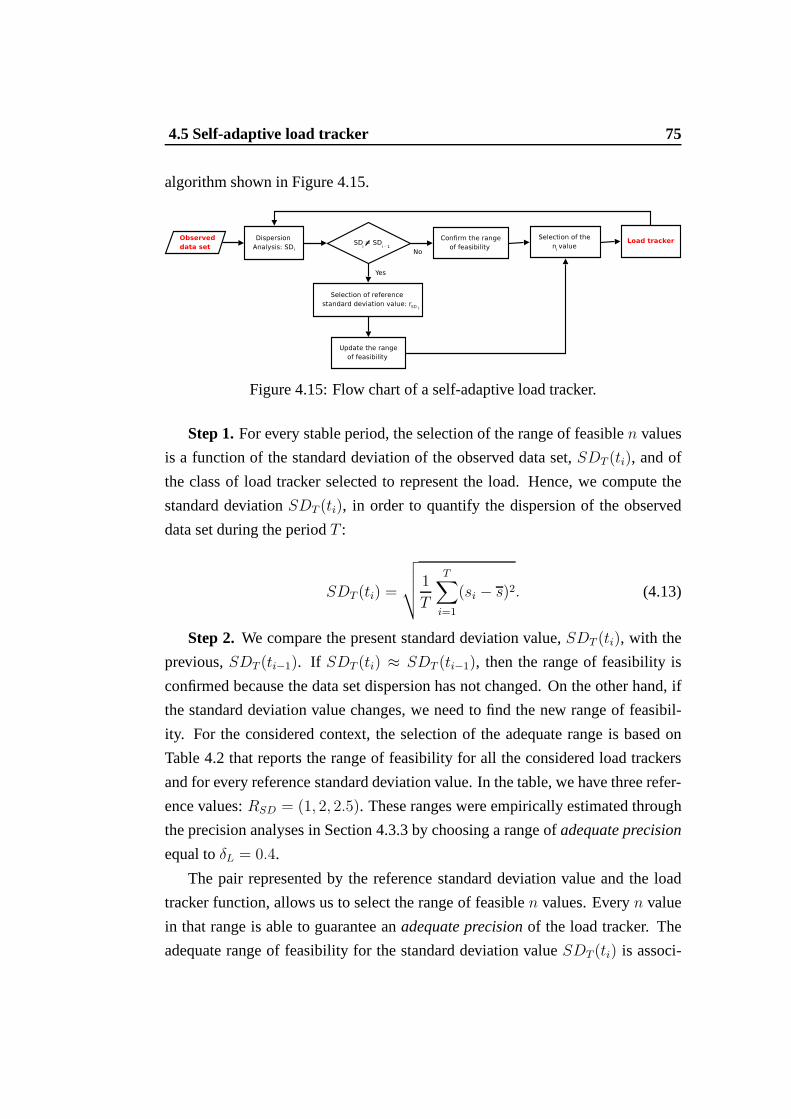
4.5 Self-adaptive load tracker 75
algorithm shown in Figure 4.15.
Figure 4.15: Flow chart of a self-adaptive load tracker.
Step 1.For every stable period, the selection of the range of feasible n values
is a function of the standard deviation of the observed data set, SDT (ti), and of
the class of load tracker selected to represent the load. Hence, we compute the
standard deviationSDT (ti), in order to quantify the dispersion of the observed
data set during the periodT :
SDT (ti) =
√
√
√
√
1
T
T∑
i=1
(si − s)2. (4.13)
Step 2. We compare the present standard deviation value,SDT (ti), with the
previous,SDT (ti−1). If SDT (ti) ≈ SDT (ti−1), then the range of feasibility is
confirmed because the data set dispersion has not changed. Onthe other hand, if
the standard deviation value changes, we need to find the new range of feasibil-
ity. For the considered context, the selection of the adequate range is based on
Table 4.2 that reports the range of feasibility for all the considered load trackers
and for every reference standard deviation value. In the table, we have three refer-
ence values:RSD = (1, 2, 2.5). These ranges were empirically estimated through
the precision analyses in Section 4.3.3 by choosing a range of adequate precision
equal toδL = 0.4.
The pair represented by the reference standard deviation value and the load
tracker function, allows us to select the range of feasiblen values. Everyn value
in that range is able to guarantee anadequate precisionof the load tracker. The
adequate range of feasibility for the standard deviation value SDT (ti) is associ-
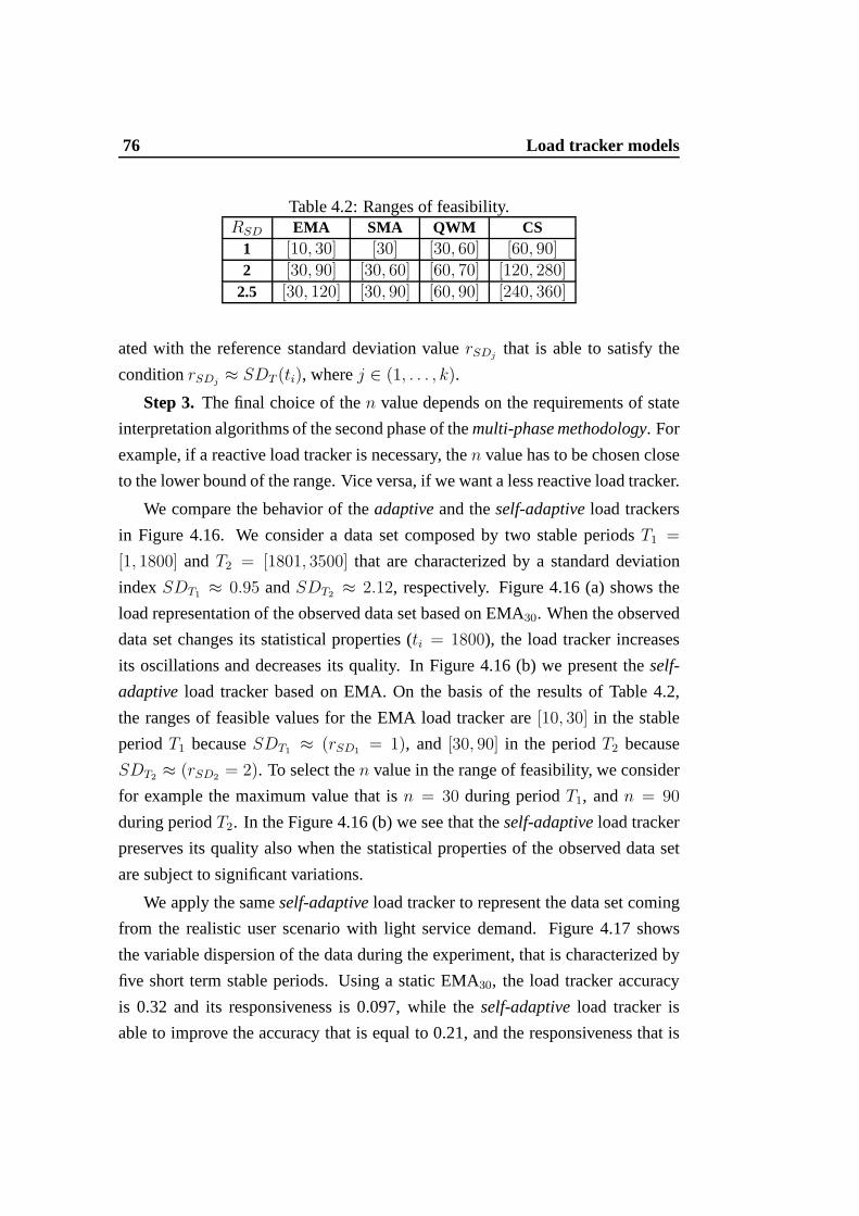
76 Load tracker models
Table 4.2: Ranges of feasibility.RSD EMA SMA QWM CS
1 [10, 30] [30] [30, 60] [60, 90]2 [30, 90] [30, 60] [60, 70] [120, 280]
2.5 [30, 120] [30, 90] [60, 90] [240, 360]
ated with the reference standard deviation valuerSDjthat is able to satisfy the
conditionrSDj≈ SDT (ti), wherej ∈ (1, . . . , k).
Step 3. The final choice of then value depends on the requirements of state
interpretation algorithms of the second phase of themulti-phase methodology. For
example, if a reactive load tracker is necessary, then value has to be chosen close
to the lower bound of the range. Vice versa, if we want a less reactive load tracker.
We compare the behavior of theadaptiveand theself-adaptiveload trackers
in Figure 4.16. We consider a data set composed by two stable periodsT1 =
[1, 1800] and T2 = [1801, 3500] that are characterized by a standard deviation
index SDT1≈ 0.95 andSDT2
≈ 2.12, respectively. Figure 4.16 (a) shows the
load representation of the observed data set based on EMA30. When the observed
data set changes its statistical properties (ti = 1800), the load tracker increases
its oscillations and decreases its quality. In Figure 4.16 (b) we present theself-
adaptiveload tracker based on EMA. On the basis of the results of Table4.2,
the ranges of feasible values for the EMA load tracker are[10, 30] in the stable
periodT1 becauseSDT1≈ (rSD1
= 1), and [30, 90] in the periodT2 because
SDT2≈ (rSD2
= 2). To select then value in the range of feasibility, we consider
for example the maximum value that isn = 30 during periodT1, andn = 90
during periodT2. In the Figure 4.16 (b) we see that theself-adaptiveload tracker
preserves its quality also when the statistical propertiesof the observed data set
are subject to significant variations.
We apply the sameself-adaptiveload tracker to represent the data set coming
from the realistic user scenario with light service demand.Figure 4.17 shows
the variable dispersion of the data during the experiment, that is characterized by
five short term stable periods. Using a static EMA30, the load tracker accuracy
is 0.32 and its responsiveness is 0.097, while theself-adaptiveload tracker is
able to improve the accuracy that is equal to 0.21, and the responsiveness that is
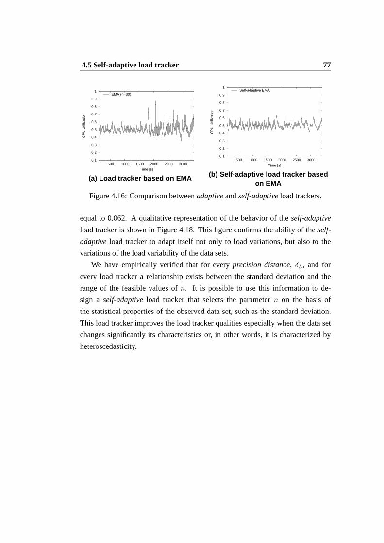
4.5 Self-adaptive load tracker 77
0.1
0.2
0.3
0.4
0.5
0.6
0.7
0.8
0.9
1
500 1000 1500 2000 2500 3000
CP
U U
tiliz
atio
n
Time [s]
EMA (n=30)
(a) Load tracker based on EMA
0.1
0.2
0.3
0.4
0.5
0.6
0.7
0.8
0.9
1
500 1000 1500 2000 2500 3000
CP
U U
tiliz
atio
n
Time [s]
Self-adaptive EMA
(b) Self-adaptive load tracker basedon EMA
Figure 4.16: Comparison betweenadaptiveandself-adaptiveload trackers.
equal to 0.062. A qualitative representation of the behavior of the self-adaptive
load tracker is shown in Figure 4.18. This figure confirms the ability of the self-
adaptiveload tracker to adapt itself not only to load variations, butalso to the
variations of the load variability of the data sets.
We have empirically verified that for everyprecision distance, δL, and for
every load tracker a relationship exists between the standard deviation and the
range of the feasible values ofn. It is possible to use this information to de-
sign a self-adaptiveload tracker that selects the parametern on the basis of
the statistical properties of the observed data set, such asthe standard deviation.
This load tracker improves the load tracker qualities especially when the data set
changes significantly its characteristics or, in other words, it is characterized by
heteroscedasticity.
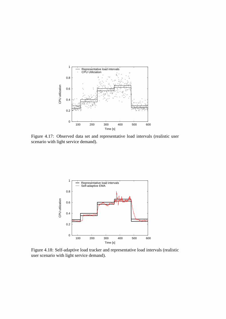
0
0.2
0.4
0.6
0.8
1
100 200 300 400 500 600
CP
U u
tiliz
atio
n
Time [s]
Representative load intervalsCPU Utilization
Figure 4.17: Observed data set and representative load intervals (realistic userscenario with light service demand).
0
0.2
0.4
0.6
0.8
1
100 200 300 400 500 600
CP
U u
tiliz
atio
n
Time [s]
Representative load intervalsSelf-adaptive EMA
Figure 4.18: Self-adaptive load tracker and representative load intervals (realisticuser scenario with light service demand).
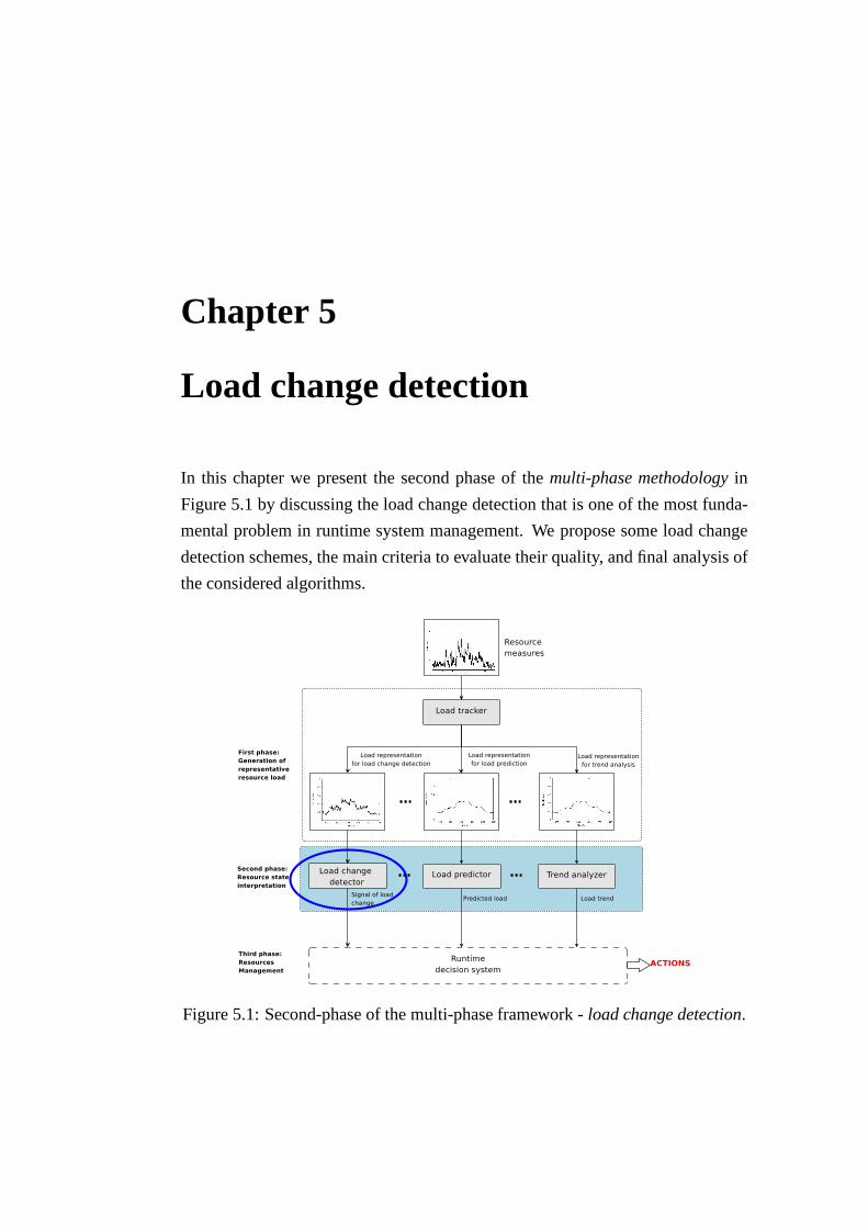
Chapter 5
Load change detection
In this chapter we present the second phase of themulti-phase methodologyin
Figure 5.1 by discussing the load change detection that is one of the most funda-
mental problem in runtime system management. We propose some load change
detection schemes, the main criteria to evaluate their quality, and final analysis of
the considered algorithms.
Figure 5.1: Second-phase of the multi-phase framework -load change detection.

80 Load change detection
5.1 Problem definition
One of the key-points for supportingadaptiveandself-adaptivemechanisms is
the ability of detecting one or several changes in some characteristic properties of
the system.
Many runtime management decisions related to Internet-based services are
activated after a notification that a significant load variation has occurred in some
system resource(s). Request redirection, process migration, access control and
limitation are some examples of processes that are activated after the detection
of a significant and non-transient system load change. We call load changeany
modification in the data sets of the system that occurs eitherinstantaneously or
rapidly with respect to the period of measurement and that lasts for a significant
period.
The first signal of load change refers to a time instant at which some attributes
of the system change, while before and after that instant theproperties are sta-
ble. This notion serves as a basis for the formal descriptionof the load change
detection problem and related algorithms.
Let (x1, . . . , xn) be a sequence of a generic data set with conditional density
pθ(xi‖xi−1, . . . , x1), where1 ≤ i ≤ n. Before the (unknown) timet0 that is
assumed as the instant of the load change, namelychange detection time, the
conditional density parameterθ is constant and equal toθ0. After t0 the same
parameter is equal toθ1. The on-line problem is to detect the occurrence of the
change as soon as possible, with a minimum or null rate of false alarms beforet0.
The detection in the increasing direction of the data value,is signaled by achange
detection rule, which usually has the form:
gi(x1, . . . , xi) ≥ χ, 1 ≤ i ≤ n (5.1)
whereχ is a threshold,gi is a parametric function at timei, namely thestate
representation function. Its change detection timet0 is defined as:
t0 = inf{i : gi(x1, . . . , xi) ≥ χ}, 1 ≤ i ≤ n (5.2)
while a detection in the opposite direction is signaled by:
t0 = inf{i : gi(x1, . . . , xi) ≤ χ}, 1 ≤ i ≤ n (5.3)

5.2 Algorithms for load change detection 81
wheret0 corresponds to the inferior extreme (inf ) of the set of thei values that
correspond to the time instants in which thechange detection ruleis verified.
5.2 Algorithms for load change detection
Several algorithms exist for solving the load change detection problem in different
contexts. For the Internet-based systems, we consider the threshold-based and
CUSUM algorithms. Both share the common trait of requiring areliable load
representation of the resource load, even if they are characterized by different
properties.
5.2.1 Single threshold-based scheme
The basic single threshold algorithm for load change detection defines a thresh-
old for a resource load, and signals a load variation when thelast observed data
value overcomes that threshold. This model has been widely adopted (just to cite
few examples in [81, 82, 89]), and its oscillatory risks are well known especially
in highly variable environments (e.g., vicious cycles in request distribution and
replica placement [20]). The risks of false alarms can be reduced by using mul-
tiple thresholds, by signaling an alarm only when multiple observed values over-
come the threshold, by augmenting the observation period, and so on. Because
of in our methodology the load state is represented by the load tracker values
(l1, l2, . . . , ln), we consider thestate representation functiongi equal to:
gi = li, 1 ≤ i ≤ n (5.4)
A load change detection in the growth direction of the load state is signaled
when the load state verifies the followingchange detection rule:
gi−1 < χ ∧ gi > χ (5.5)
while in the opposite direction:
gi−1 > χ ∧ gi < χ (5.6)

82 Load change detection
whereχ is the threshold value. Consequently, thechange detection timet0 is equal
to:
t0 = {i : (gi−1 < χ ∧ gi > χ)} (5.7)
or, for a load change detection in the decrease direction of the load state,t0 is
equal to:
t0 = {i : (gi−1 > χ ∧ gi < χ)} (5.8)
A valid load change detector detects as soon as possible a change of repre-
sentative load over or under the thresholdχ, but it limits or avoids false load
detections.
5.2.2 CUSUM scheme
The CUSUM algorithm is adopted in statistical control to detect mean value
changes of a stochastic process [11]. This scheme relies on the observation that if
a change occurs, the probability distribution of the data set changes as well. The
CUSUM algorithm requires a parametric model for the observed data, such as the
AR and ARIMA models, so that the probability density function can monitor the
data sequence. As demonstrated in Chapter 2, Internet-based systems are very
dynamic and complicated entities, and the construction of these parametric mod-
els is still an open problem. In this thesis we use the load tracker functions for
modeling the data set because they are robust and do not require a sophisticated
tuning of the parameters.
Let (l1, l2, . . . , ln) be a sequence of load tracker values that are characterized
by:
• conditional probability densityfθ0(li/li−1, . . . , l1) before the change time
t0, whereθ0 is the parameter vector of the load tracker value segmentLT0
beforet0;
• a conditional probability densityfθ1(li/li−1, . . . , l1) aftert0 whereθ1 is the
parameter vector of the segmentLT1 after this instant.
Let LT i1 be the sum of the logarithms of the successive likelihood ratios [11]:

5.3 Evaluation: reactivity and delay error 83
LT i1 =
∑
1≤j≤i
ki =∑
1≤j≤i
logfθ0
(li/li−1, . . . , l1)
fθ1(li/li−1, . . . , l1)
, 1 ≤ i ≤ n (5.9)
Thestate representation functiongi is defined as:
gi = LT i1 − min
1≤j≤iLT j
1 (5.10)
and the correspondingchange detection timefor a load change detection in the
increase direction of the load state is:
t0 = min{i : gi ≤ χ} (5.11)
or for a load change detection in the opposite direction:
t0 = min{i : gi ≥ χ} (5.12)
whereχ is a given threshold.
In case of a CUSUM algorithm, the selection of the threshold is generally
based on the Kullback-Leibler distance between two probability densitiesfθ0and
fθ1of a load tracker values(l1, . . . , ln), defined as:
K(θ0, θ1) =
∫
lnfθ0
(l)
fθ1(l)
fθ0(l)dl (5.13)
From [11] it is known that the detection delay is inversely proportional to
the Kullback-Leibler distance. Ifχ is the threshold for detection, the relationship
betweenχ and the Kullback-Leibler distance can be expressed as:
K(θ1, θ0) =χ
τ(5.14)
whereτ is the mean delay for detection. From Equation 5.14 we can writeχ ≈ τ ∗
K(θ1, θ0) and consequently the Kullback-Leibler distance can be usedto choose
the thresholdχ of the CUSUM algorithm.
5.3 Evaluation: reactivity and delay error
Two properties characterize a good load change detector: the rapidity in signaling
a significant load change, and the ability to discern a steadyload change from

84 Load change detection
a transient change. These two properties are conflicting, because a detector that
is able to quickly signal load changes, has also higher chances of mistaking a
transient load spike for a steady load change. Figures 5.2 (a) and (b) show a
representation of a general load change detection model based on the observed
data set and the load tracker where the thresholdχ is set to 0.4. From these
figures, we observe the two possible types of false detections:
• The excess of oscillations of a data set around the threshold valueχ causes
many false alarms. This type of error is extremely evident inthe case of the
observed data set (Figure 5.2 (a)), but also in the case of a highly responsive
load change detector such as QWM10 (Figure 5.2 (b)).
• The excess of smoothing of a load tracker may cause a delay insignaling a
variation of load conditions. This kind of errors is evidentin the case of a
smoothed load change detector, such as QWM60 (Figure 5.2 (b)).
The load change detection is a typical problem where we prefer a load tracker
that solves the trade-off between too much reactivity causing false alarms and ex-
cessive smoothness causing delays. In other terms, we do notwant a too accurate
or too responsive load tracker, but one having “adequate” precision. If there are
multiple adequate load trackers, the best choice depends ona preference given to
responsiveness or accuracy.
The ability of a load change detector is to detect as soon as possible a change
of representative load intervals, that were presented in Section 4.2.2, over or under
the thresholdχ. Errors are caused when the detector signals an opposite load state
of the functiongi that is, when
(TUI < χ ∧ gi > χ) ∨ (T L
I > χ ∧ gi < χ) (5.15)
whereTUI andTL
I are the upper and lower bounds of the representative load in-
tervals andgi is state representation functionat timeti that is equal toli for the
single threshold model (as shown in Equation 5.4) andLT i1 − min
1≤j≤iLT j
1 for the
CUSUM model (as shown in Equation 5.10). As shown in Figure 5.2 two possible
sources of errors exist that we define as:delayandreactivityerrors.
Thedelay erroris the sum of wrong observations occurring between a change
of approximate confidence interval and the first right observation recognizing the
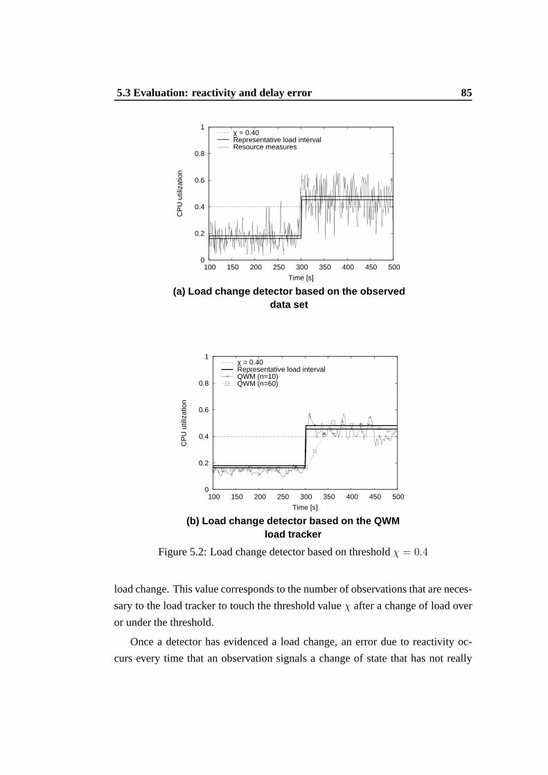
5.3 Evaluation: reactivity and delay error 85
0
0.2
0.4
0.6
0.8
1
100 150 200 250 300 350 400 450 500
CP
U u
tiliz
atio
n
Time [s]
χ = 0.40Representative load intervalResource measures
(a) Load change detector based on the observeddata set
0
0.2
0.4
0.6
0.8
1
100 150 200 250 300 350 400 450 500
CP
U u
tiliz
atio
n
Time [s]
χ = 0.40Representative load intervalQWM (n=10)QWM (n=60)
(b) Load change detector based on the QWMload tracker
Figure 5.2: Load change detector based on thresholdχ = 0.4
load change. This value corresponds to the number of observations that are neces-
sary to the load tracker to touch the threshold valueχ after a change of load over
or under the threshold.
Once a detector has evidenced a load change, an error due to reactivity oc-
curs every time that an observation signals a change of statethat has not really
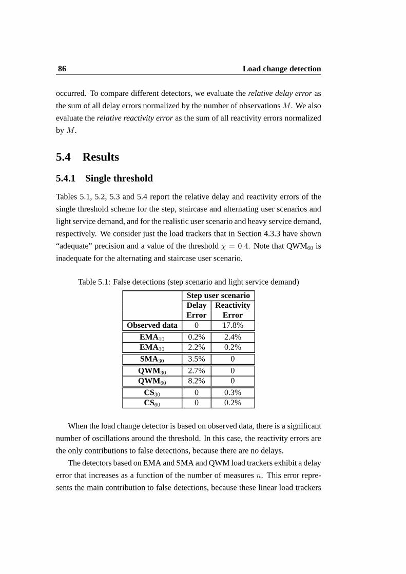
86 Load change detection
occurred. To compare different detectors, we evaluate therelative delay erroras
the sum of all delay errors normalized by the number of observationsM . We also
evaluate therelative reactivity erroras the sum of all reactivity errors normalized
by M .
5.4 Results
5.4.1 Single threshold
Tables 5.1, 5.2, 5.3 and 5.4 report the relative delay and reactivity errors of the
single threshold scheme for the step, staircase and alternating user scenarios and
light service demand, and for the realistic user scenario and heavy service demand,
respectively. We consider just the load trackers that in Section 4.3.3 have shown
“adequate” precision and a value of the thresholdχ = 0.4. Note that QWM60 is
inadequate for the alternating and staircase user scenario.
Table 5.1: False detections (step scenario and light service demand)
Step user scenarioDelay ReactivityError Error
Observed data 0 17.8%
EMA 10 0.2% 2.4%EMA 30 2.2% 0.2%
SMA30 3.5% 0
QWM 30 2.7% 0QWM 60 8.2% 0
CS30 0 0.3%CS60 0 0.2%
When the load change detector is based on observed data, there is a significant
number of oscillations around the threshold. In this case, the reactivity errors are
the only contributions to false detections, because there are no delays.
The detectors based on EMA and SMA and QWM load trackers exhibit a delay
error that increases as a function of the number of measuresn. This error repre-
sents the main contribution to false detections, because these linear load trackers

Single threshold 87
Table 5.2: False detections (staircase scenario and light service demand)
Staircase user scenarioDelay ReactivityError Error
Observed data 0 13.8%
EMA 10 2.0% 0.6%EMA 30 3.3% 0
SMA30 5.8% 0
QWM 30 4.2% 0QWM 60 X X
CS30 0.5% 1.9%CS60 0.8% 1.5%
seem smoothed enough to avoid reactivity errors unless for too small set ofn val-
ues. The opposite is true for load change detectors based on CS load trackers:
they are affected by very low delay errors, but by high reactivity errors especially
for few n values. These load trackers are characterized by a decreasing number
of oscillations with higher values ofn. These oscillations are the main reason of
false detections.
An overall evaluation of the results in Tables 5.1, 5.2 and 5.3 shows that, for a
light service demand, the best detectors are based on the non-linear CS60 and on
the linear EMA30 functions. Both of them are characterized by low percentages of
false detections, that are always lower than 5% even in the most severe alternating
user scenario.
Similar considerations hold true also when we consider the more jittery heavy
service demand shown in Table 5.4. This table reports only the load trackers with
“adequate” precision, as determined in Section 4.3.3. The main differenc with
respect to the user scenarios based on a light service demandis the augmented
number of errors caused by the higher dispersion of the resource measures. As a
consequence, the best load trackers (EMA60, QWM60 and CS240) for supporting
load change detection need a larger amount of measured values than that required
for the user scenarios with a light service demand.
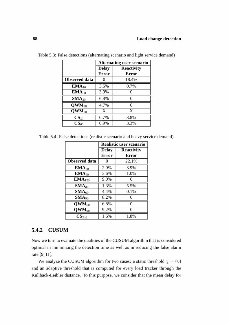
88 Load change detection
Table 5.3: False detections (alternating scenario and light service demand)
Alternating user scenarioDelay ReactivityError Error
Observed data 0 18.4%
EMA 10 3.6% 0.7%EMA 30 3.9% 0
SMA30 6.8% 0
QWM 30 4.7% 0QWM 60 X X
CS30 0.7% 3.8%CS60 0.9% 3.3%
Table 5.4: False detections (realistic scenario and heavy service demand)
Realistic user scenarioDelay ReactivityError Error
Observed data 0 22.1%
EMA 60 2.0% 3.9%EMA 90 3.6% 1.0%EMA 120 9.0% 0
SMA30 1.3% 5.5%SMA60 4.4% 0.1%SMA90 8.2% 0
QWM 60 6.8% 0QWM 90 9.2% 0
CS240 1.6% 1.8%
5.4.2 CUSUM
Now we turn to evaluate the qualities of the CUSUM algorithm that is considered
optimal in minimizing the detection time as well as in reducing the false alarm
rate [9,11].
We analyze the CUSUM algorithm for two cases: a static threshold χ = 0.4
and an adaptive threshold that is computed for every load tracker through the
Kullback-Leibler distance. To this purpose, we consider that the mean delay for
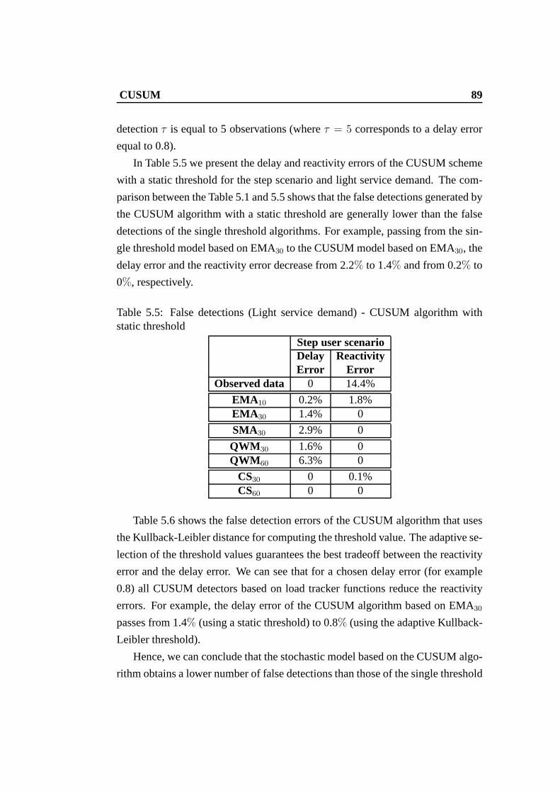
CUSUM 89
detectionτ is equal to 5 observations (whereτ = 5 corresponds to a delay error
equal to 0.8).
In Table 5.5 we present the delay and reactivity errors of theCUSUM scheme
with a static threshold for the step scenario and light service demand. The com-
parison between the Table 5.1 and 5.5 shows that the false detections generated by
the CUSUM algorithm with a static threshold are generally lower than the false
detections of the single threshold algorithms. For example, passing from the sin-
gle threshold model based on EMA30 to the CUSUM model based on EMA30, the
delay error and the reactivity error decrease from 2.2% to 1.4% and from 0.2% to
0%, respectively.
Table 5.5: False detections (Light service demand) - CUSUM algorithm withstatic threshold
Step user scenarioDelay ReactivityError Error
Observed data 0 14.4%
EMA 10 0.2% 1.8%EMA 30 1.4% 0
SMA30 2.9% 0
QWM 30 1.6% 0QWM 60 6.3% 0
CS30 0 0.1%CS60 0 0
Table 5.6 shows the false detection errors of the CUSUM algorithm that uses
the Kullback-Leibler distance for computing the thresholdvalue. The adaptive se-
lection of the threshold values guarantees the best tradeoff between the reactivity
error and the delay error. We can see that for a chosen delay error (for example
0.8) all CUSUM detectors based on load tracker functions reduce the reactivity
errors. For example, the delay error of the CUSUM algorithm based on EMA30passes from 1.4% (using a static threshold) to 0.8% (using the adaptive Kullback-
Leibler threshold).
Hence, we can conclude that the stochastic model based on theCUSUM algo-
rithm obtains a lower number of false detections than those of the single threshold

90 Load change detection
scheme.
Table 5.6: False detections (Step scenario and light service demand) - CUSUMalgorithm with Kullback-Leibler threshold
Step user scenarioDelay ReactivityError Error
Observed data 0.8% 10%
EMA 10 0.8% 0.5%EMA 30 0.8% 0
SMA30 0.8% 0
QWM 30 0.8% 0QWM 60 0.8% 0
CS30 0.8% 0CS60 0.8% 0
5.5 Conclusions
In this chapter we have discussed theload change detectionmodule, whose pur-
pose is to detect non transient modifications of the statistical properties in resource
measures. We have proposed two stochastic models for the evaluation of load state
changes:
• a single threshold scheme;
• a CUSUM scheme with static andadaptivethresholds.
We have evaluated the reactivity and delay error of the proposed models for
different scenarios. The analyses point out some interesting results, which are
outlined below.
• There are several causes that contribute to the overall error: in the linear
case, the contribution is almost entirely due to delays; in the non linear
case, the contribution is almost entirely due to excessive reactivity.

5.5 Conclusions 91
• If the runtime management system needs a reactive load representation,
load change detectionmodels based on the cubic spline are selected. Al-
ternatively, a detector based on EMA models is the best choice when the
run-time management system needs a precise load representation that has
not to be affected by many false alarms.
• The bestload change detectionmodel is the CUSUM algorithm with an
adaptivethreshold, because it is able to minimize the delay and to avoid
false detections due to transient load variations.

Chapter 6
Load trend
The load trend analysis represents an innovative representation model of the sec-
ond phase of themulti-phase methodology(Figure 6.1). We think that most of the
runtime algorithms for supporting the management of distributed systems should
not consider just the ”absolute” values coming from the loadrepresentation, but
they should take decisions by evaluating the behavioral trend of the system state
in the past observation interval. Theload trendcan give an importantgeometric
interpretationabout the resource behavior with respect to the past load tracker
values, for example, whether it is increasing, decreasing or oscillating.
6.1 Problem definition
A typical condition thatload trendmodels have to manage can be described as
follows. Let us assume that the values of two data sets are equal to [0.4, 0.5,
0.6] and [0.8, 0.7, 0.6], respectively. Although the last observation for both data
sets is equal to 0.6, the data sets are characterized by two completely different
conditions, because the values of the data set 2 are decreasing while the values of
the data set 1 keep increasing.
More formally, the load trend model is a functionT (Xn, m) that takes into
account :
• n values of the stochastic data setXn = (xi−(n−1), . . . , xi);
• the numberm of the last values of the observed data set that are utilized for
the load trend evaluation,m ≤ n.
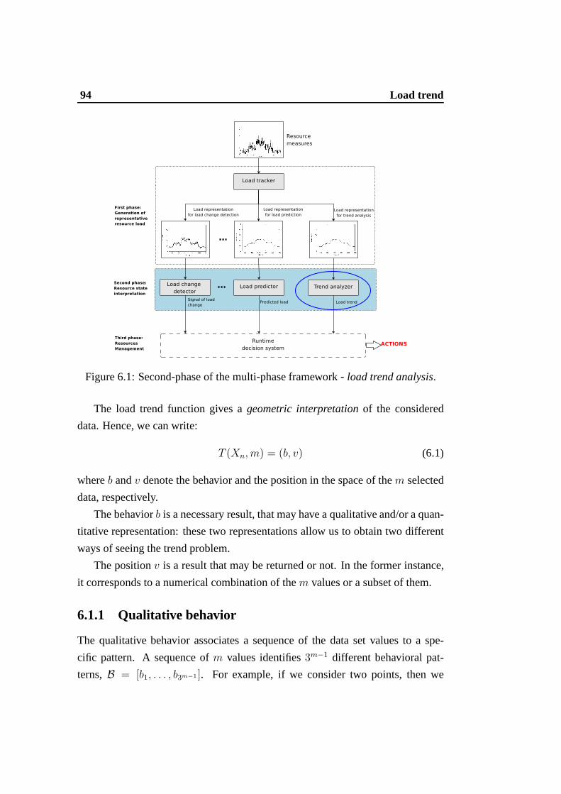
94 Load trend
Figure 6.1: Second-phase of the multi-phase framework -load trend analysis.
The load trend function gives ageometric interpretationof the considered
data. Hence, we can write:
T (Xn, m) = (b, v) (6.1)
whereb andv denote the behavior and the position in the space of them selected
data, respectively.
The behaviorb is a necessary result, that may have a qualitative and/or a quan-
titative representation: these two representations allowus to obtain two different
ways of seeing the trend problem.
The positionv is a result that may be returned or not. In the former instance,
it corresponds to a numerical combination of them values or a subset of them.
6.1.1 Qualitative behavior
The qualitative behavior associates a sequence of the data set values to a spe-
cific pattern. A sequence ofm values identifies3m−1 different behavioral pat-
terns,B = [b1, . . . , b3m−1 ]. For example, if we consider two points, then we
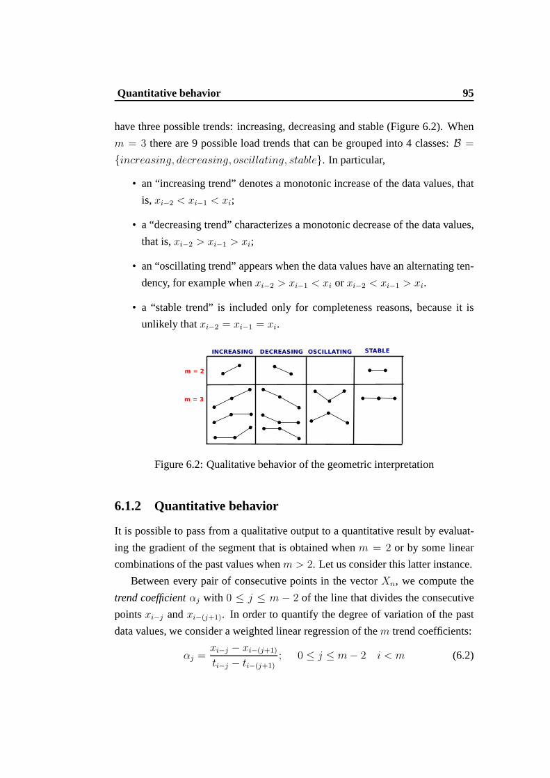
Quantitative behavior 95
have three possible trends: increasing, decreasing and stable (Figure 6.2). When
m = 3 there are 9 possible load trends that can be grouped into 4 classes:B =
{increasing, decreasing, oscillating, stable}. In particular,
• an “increasing trend” denotes a monotonic increase of the data values, that
is, xi−2 < xi−1 < xi;
• a “decreasing trend” characterizes a monotonic decrease of the data values,
that is,xi−2 > xi−1 > xi;
• an “oscillating trend” appears when the data values have analternating ten-
dency, for example whenxi−2 > xi−1 < xi or xi−2 < xi−1 > xi.
• a “stable trend” is included only for completeness reasons, because it is
unlikely thatxi−2 = xi−1 = xi.
Figure 6.2: Qualitative behavior of the geometric interpretation
6.1.2 Quantitative behavior
It is possible to pass from a qualitative output to a quantitative result by evaluat-
ing the gradient of the segment that is obtained whenm = 2 or by some linear
combinations of the past values whenm > 2. Let us consider this latter instance.
Between every pair of consecutive points in the vectorXn, we compute the
trend coefficientαj with 0 ≤ j ≤ m − 2 of the line that divides the consecutive
pointsxi−j andxi−(j+1). In order to quantify the degree of variation of the past
data values, we consider a weighted linear regression of them trend coefficients:
αj =xi−j − xi−(j+1)
ti−j − ti−(j+1); 0 ≤ j ≤ m − 2 i < m (6.2)
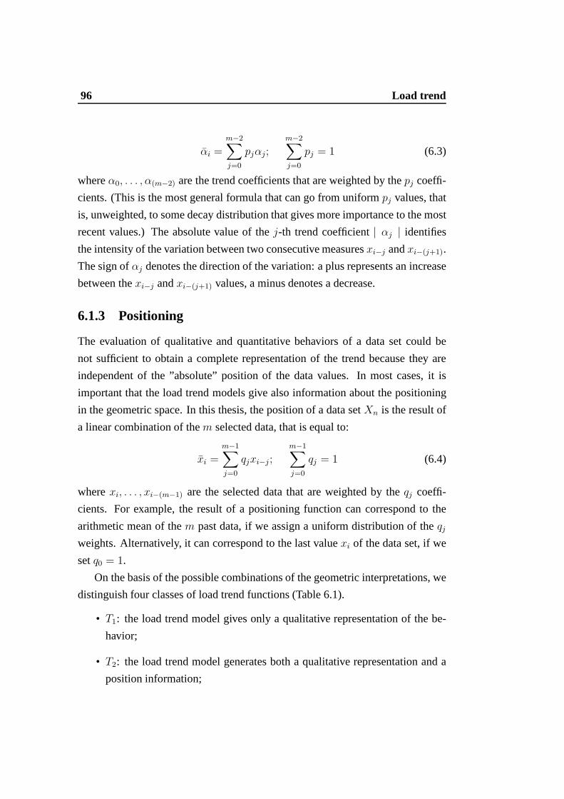
96 Load trend
αi =
m−2∑
j=0
pjαj;
m−2∑
j=0
pj = 1 (6.3)
whereα0, . . . , α(m−2) are the trend coefficients that are weighted by thepj coeffi-
cients. (This is the most general formula that can go from uniform pj values, that
is, unweighted, to some decay distribution that gives more importance to the most
recent values.) The absolute value of thej-th trend coefficient| αj | identifies
the intensity of the variation between two consecutive measuresxi−j andxi−(j+1).
The sign ofαj denotes the direction of the variation: a plus represents anincrease
between thexi−j andxi−(j+1) values, a minus denotes a decrease.
6.1.3 Positioning
The evaluation of qualitative and quantitative behaviors of a data set could be
not sufficient to obtain a complete representation of the trend because they are
independent of the ”absolute” position of the data values. In most cases, it is
important that the load trend models give also information about the positioning
in the geometric space. In this thesis, the position of a datasetXn is the result of
a linear combination of them selected data, that is equal to:
xi =
m−1∑
j=0
qjxi−j ;
m−1∑
j=0
qj = 1 (6.4)
wherexi, . . . , xi−(m−1) are the selected data that are weighted by theqj coeffi-
cients. For example, the result of a positioning function can correspond to the
arithmetic mean of them past data, if we assign a uniform distribution of theqj
weights. Alternatively, it can correspond to the last valuexi of the data set, if we
setq0 = 1.
On the basis of the possible combinations of the geometric interpretations, we
distinguish four classes of load trend functions (Table 6.1).
• T1: the load trend model gives only a qualitative representation of the be-
havior;
• T2: the load trend model generates both a qualitative representation and a
position information;
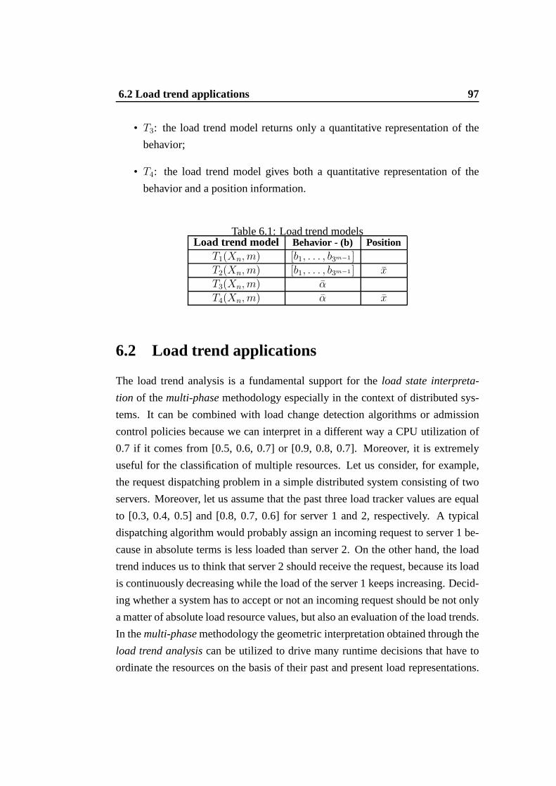
6.2 Load trend applications 97
• T3: the load trend model returns only a quantitative representation of the
behavior;
• T4: the load trend model gives both a quantitative representation of the
behavior and a position information.
Table 6.1: Load trend modelsLoad trend model Behavior - (b) Position
T1(Xn, m) [b1, . . . , b3m−1 ]T2(Xn, m) [b1, . . . , b3m−1 ] xT3(Xn, m) αT4(Xn, m) α x
6.2 Load trend applications
The load trend analysis is a fundamental support for theload state interpreta-
tion of themulti-phasemethodology especially in the context of distributed sys-
tems. It can be combined with load change detection algorithms or admission
control policies because we can interpret in a different waya CPU utilization of
0.7 if it comes from [0.5, 0.6, 0.7] or [0.9, 0.8, 0.7]. Moreover, it is extremely
useful for the classification of multiple resources. Let us consider, for example,
the request dispatching problem in a simple distributed system consisting of two
servers. Moreover, let us assume that the past three load tracker values are equal
to [0.3, 0.4, 0.5] and [0.8, 0.7, 0.6] for server 1 and 2, respectively. A typical
dispatching algorithm would probably assign an incoming request to server 1 be-
cause in absolute terms is less loaded than server 2. On the other hand, the load
trend induces us to think that server 2 should receive the request, because its load
is continuously decreasing while the load of the server 1 keeps increasing. Decid-
ing whether a system has to accept or not an incoming request should be not only
a matter of absolute load resource values, but also an evaluation of the load trends.
In themulti-phasemethodology the geometric interpretation obtained through the
load trend analysiscan be utilized to drive many runtime decisions that have to
ordinate the resources on the basis of their past and presentload representations.
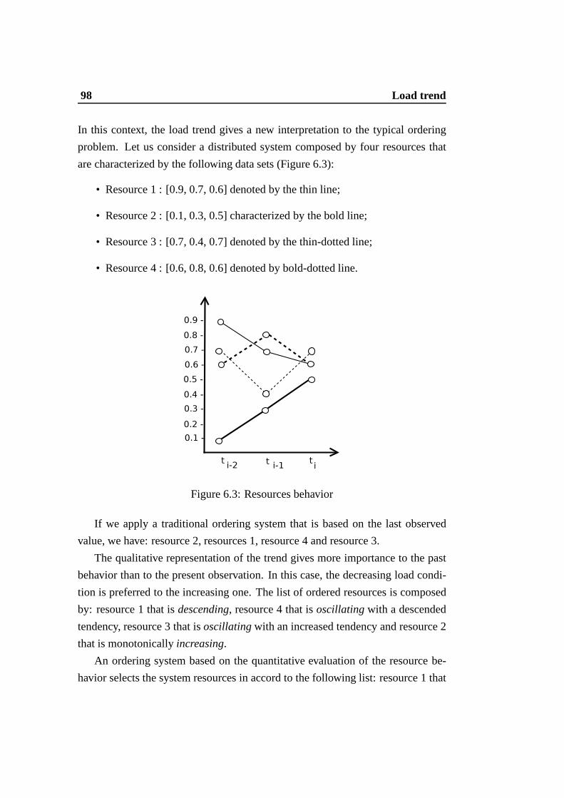
98 Load trend
In this context, the load trend gives a new interpretation tothe typical ordering
problem. Let us consider a distributed system composed by four resources that
are characterized by the following data sets (Figure 6.3):
• Resource 1 : [0.9, 0.7, 0.6] denoted by the thin line;
• Resource 2 : [0.1, 0.3, 0.5] characterized by the bold line;
• Resource 3 : [0.7, 0.4, 0.7] denoted by the thin-dotted line;
• Resource 4 : [0.6, 0.8, 0.6] denoted by bold-dotted line.
Figure 6.3: Resources behavior
If we apply a traditional ordering system that is based on thelast observed
value, we have: resource 2, resources 1, resource 4 and resource 3.
The qualitative representation of the trend gives more importance to the past
behavior than to the present observation. In this case, the decreasing load condi-
tion is preferred to the increasing one. The list of ordered resources is composed
by: resource 1 that isdescending, resource 4 that isoscillatingwith a descended
tendency, resource 3 that isoscillatingwith an increased tendency and resource 2
that is monotonicallyincreasing.
An ordering system based on the quantitative evaluation of the resource be-
havior selects the system resources in accord to the following list: resource 1 that

6.3 Weighted-Trend Algorithm 99
hasα = −0.15, resource 3 and 4 that are characterized byα = 0 and resource 2
that hasα = +0.2.
A hybrid interpretation of the load trend, that utilizes both the qualitative
evaluation and the position information, obtains the following list of ordered re-
sources: resource 1, resource 3, resource 2, and resource 4.
As we have seen, the load trend opens a wide spectrum of novel possibilities
of which only a subset has been investigated in this thesis.
6.3 Weighted-Trend Algorithm
In this section we propose an example of load trend stochastic model, namely
Weighted Trend, that is a functionT4(LT (Sn(ti)), 3) = (α, l) that is based on a
quantitative representation and on a position-based information of the load tracker
values. This function is specifically designed for the generation of a runtime trend
representation in the context of Internet-based systems.
The degree of variation of the past load tracker values is evaluated with respect
to the weighted linear regression of the past3 values and2 trend coefficients, that
is:
αj =li−j − li−(j+1)
ti−j − ti−(j+1)
; 0 ≤ j ≤ 1 (6.5)
αi = p0α0 + p1α1; p0 = p1 = 0.5 (6.6)
where[α0, α1] are the trend coefficients and the weights are uniform.
The position value is evaluated with respect to a linear combination of the past
3 load tracker values, weighted by a decay distribution ofpj values, that is:
li =2
∑
j=0
qjli−j ; q0 = 0.5; q1 = 0.3; q2 = 0.2; (6.7)
We will describe an application of this Weighted-Trend function to the dis-
patching policy of the distributed system in Section 8.4.

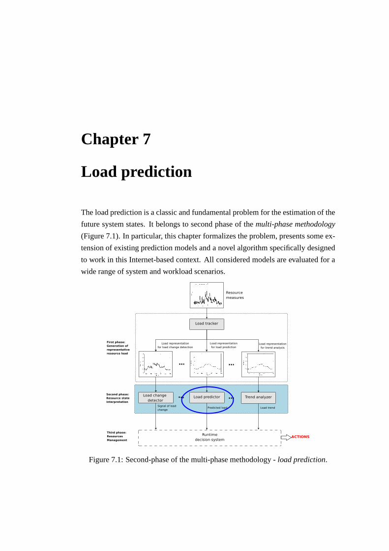
Chapter 7
Load prediction
The load prediction is a classic and fundamental problem forthe estimation of the
future system states. It belongs to second phase of themulti-phase methodology
(Figure 7.1). In particular, this chapter formalizes the problem, presents some ex-
tension of existing prediction models and a novel algorithmspecifically designed
to work in this Internet-based context. All considered models are evaluated for a
wide range of system and workload scenarios.
Figure 7.1: Second-phase of the multi-phase methodology -load prediction.

102 Load prediction
7.1 Problem definition
In the multi-phase methodology, the prediction models workon the basis of an
ordered set of historical information provided by the load tracker functions. A
prediction is the output of a function conditioned onLT (−→Sn(ti)) : R
n → R,
li+k = LPk(−→Lq(ti)) + ǫi, in which LPk() is a function capturing the predictable
component of the load tracker values vector−→Lq(ti) = (li−q, . . . , li) at timeti, ǫi
models the possible noise, andk denotes the number of steps in the future, namely
prediction window.
There is a plethora of prediction models that aim to time series forecasting. We
cite just the most important classes: linear time series [42], neural network [97],
wavelet analysis [83], Support Vector Machines [37], Fuzzysystems [97]. The
choice of the most appropriate prediction model depends on the requirements of
the application context. Most of the prediction models are designed for off-line
applications. This is the case of the genetic algorithms, neural networks, SVM,
Fuzzy systems that may achieve a valid prediction quality after a long execution
times. The most complex models are expensive to fit, hence it is difficult or impos-
sible to use them in a dynamic and runtime environment such asthe Internet-based
system. Many runtime prediction models come from the economic field, such as
the Auto Regressive models (AR, ARMA, ARIMA) and other linear models. Con-
sequently, the proposal of runtime prediction models for Internet based systems is
an open issues that motivates our research.
If we consider that our focus is on runtime and short-term prediction algo-
rithms in an extremely variable and dynamic environment, wecan define the two
main properties of our interest:
Prediction quality. This is a general attribute that considers two important fea-
tures: the precision in modeling the future data set in a hypothetic stable
condition, the adaptability in following load variations when conditions are
unstable.
Prediction cost. In a runtime prediction context, the computational complexity
of the algorithm implementing a prediction model is of utmost importance.
The rationale behind these attributes is that we want an accurate prediction,
7.1 Problem definition 103
but we are also interested to the execution time to obtain it.This aspect is even
more critical in a short-term prediction context where the look ahead is of at most
few minutes.
Thanks to the multi-phase methodology, we can expect that even simple linear
predictors may be sufficient to forecast the future load of a resource. In this con-
text, we confirm previous studies [10, 71, 90] that demonstrate that even simple
linear models, such as the auto-regressive model or the linear interpolation, are
adequate for prediction when the correlation of consecutive observed data values
is high. For example, in [42] it is shown that the UNIX load average can be ac-
curately predicted with low computational cost through an auto-regressive model
that takes into account the last 16 measures (AR(16)).
The models considered in this thesis lack the learning capabilities of the more
complex prediction algorithms, but in the considered context it is mandatory to
achieve good (not necessarily optimal) predictions quickly, rather than looking
for the optimal decision in an unpredictable amount of time.
There is another important difference between the load prediction schemes
proposed in this thesis and the state-of-the art. In previous models, the vector−→Lq(ti) consists of observed data values, and the load predictors aim to forecast at
time ti+k a future observed data. On the other hand, following the multi-phase
methodology, we propose that our load predictors takes as their input a set of
load tracker values and returns a future load tracker value.In a context where the
observed data sets obtained from the load monitors of the Internet-based servers
are extremely variable, there are two reasons that justify our choice.
• The behavior of monitored resource loads appears extremely variable to the
extent that a prediction of a future observed data value is useless for taking
accurate decisions.
• Many proposed load predictors working on real measures maybe unsuitable
to support a runtime decision system because of their excessive computa-
tional complexity.
An important premise is that no prediction model can work if the analyzed
time series does not exhibit a temporal dependency and a low noise component.
104 Load prediction
The data set has to show some temporal dependency, otherwiseany prediction is
unfeasible. Theauto-correlation analysison the time series allows us to show
the presence of some time dependence and to distinguish between the possibility
of achieving long-term or just short-term prediction (as previously demonstrate
in Chapter 2). Moreover, a highly variable and noisy data setdoes not prevent
predictability, but it limits the prediction accuracy alsoin stable conditions.
The accuracy and the time interval of the prediction algorithms depend on the
auto-correlation functions (inverse Fourier transforms)of the power spectra of the
considered data set, that is,
ACF (k) =1
(n − k)σ2
n−k∑
i=1
[si − µ][si+k − µ] (7.1)
wheresi andsi+k are the values at the lagsti andti+k, µ is the mean value, and
σ2 the variance. The problem with the observed data sets that are related to the
internal system resources of Internet-based servers is that their auto-correlation
functions decay soon. As an example, we report in Figures 7.2the auto-correlation
analysis of six sets of data referring to three system resources (CPU, network and
disk utilization) in an application server and in a databaseserver of a multi-tier
Web system [19] subjected to a stable workload and heavy service demand. We
should consider that these results are representative of a very large set of data
related to the internal resources of Internet-based servers. In the Figure 7.2, a
point (tk, ACFk) denotes that the correlation between the load value observed at
time ti and that observed at timeti+k is equal toACFk. A high value of the auto-
correlation function between the data at timeti andti+k suggests that the value
at timeti may be used to predict the measure at timeti+k with some degree of
accuracy. The vice versa is true when the ACF between two points tends to zero.
There is a close relationship among the oscillatory behavior of the data, the
auto-correlation values, and the predictability: large oscillations tend to denote
rapidly falling auto-correlation functions with the consequence that a future state
is difficult to forecast through a runtime prediction model.The message from the
Figures 7.2 and all other not reported results is quite uniform and clear: indepen-
dently of the considered system resource and server, the auto-correlation functions
of the observed data sets decay steeply.
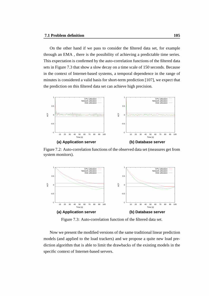
7.1 Problem definition 105
On the other hand if we pass to consider the filtered data set, for example
through an EMA , there is the possibility of achieving a predictable time series.
This expectation is confirmed by the auto-correlation functions of the filtered data
sets in Figure 7.3 that show a slow decay on a time scale of 150 seconds. Because
in the context of Internet-based systems, a temporal dependence in the range of
minutes is considered a valid basis for short-term prediction [107], we expect that
the prediction on this filtered data set can achieve high precision.
-1
-0.5
0
0.5
1
10 20 30 40 50 60 70 80 90 100
AC
F
Time [s]
CPU utilizationNetwork utilization
Disk utilization
(a) Application server
-1
-0.5
0
0.5
1
10 20 30 40 50 60 70 80 90 100
AC
F
Time [s]
CPU utilizationNetwork utilization
Disk utilization
(b) Database server
Figure 7.2: Auto-correlation functions of the observed data set (measures get fromsystem monitors).
-1
-0.5
0
0.5
1
10 20 30 40 50 60 70 80 90 100
AC
F
Time [s]
CPU utilizationNetwork utilization
Disk utilization
(a) Application server
-1
-0.5
0
0.5
1
10 20 30 40 50 60 70 80 90 100
AC
F
Time [s]
CPU utilizationNetwork utilization
Disk utilization
(b) Database server
Figure 7.3: Auto-correlation function of the filtered data set.
Now we present the modified versions of the same traditional linear prediction
models (and applied to the load trackers) and we propose a quite new load pre-
diction algorithm that is able to limit the drawbacks of the existing models in the
specific context of Internet-based servers.

106 Load prediction
7.2 Linear prediction models
We consider four main classes of linear prediction models based on historical in-
formation and auto-correlated data sets that can be adaptedto considered runtime
contexts. Moreover, we propose an original model that is designed for Internet-
based systems. In summary, we consider:
• Exponential weighted moving average (EWMA);
• Auto-regressive (AR);
• Auto-regressive integrated moving average (ARIMA);
• Linear regression (LR);
• Trend-aware regression (TAR).
Exponential Weighted Moving Average(EWMA). This model predicts the
future valuek steps ahead as the weighted average of the last data and the previ-
ously predicted value carried out onn past values:
LPk(−→Lq(ti)) = αli + (1 − α)li (7.2)
whereα is typically set to 2n+1
. The EWMA models are simple linear algorithms
that are characterized by a very low prediction cost. Their accuracy depends on
the data set characteristics: in stable conditions, they exhibit a good prediction
quality. When the data set is less stable, the prediction quality tends to decrease
as well. The main problem is that the EWMA models generates a future value
after a delay that is proportional ton, wheren is the size of the data setSi. It
is possible to modify the effects of the accuracyvsdelay trade-off of the EWMA
models through a different choice of the parametersα andn.
Auto-Regressive Model(AR). A k-step prediction through an AR model is
a weighted linear combination ofp values: thek − 1 previously predicted values
li+k−1, . . . , li+1; thep − k values of the data set(li, . . . , li−(p−k)). An AR-based
predictor at timeti can be written as:
LPk(−→Lq(ti)) = φ1li+(k−1) + · · ·+ φpli−(p−k) + ǫi (7.3)
7.2 Linear prediction models 107
whereei ∼ WN(0, σ2) is an independent and identically distributed sequence
(calledresiduals sequence), and thep linear coefficientsφ1, . . . , φp are the firstp
values of the auto-correlation function evaluated on a subset of the considered data
set. Thep order of the AR process is determined by the lag at which the partial
auto-correlation function becomes negligible [16,65]. The numberp of considered
observed data values is a parameter of the AR model, hence by AR(p) we denote
an AR predictor based onp values. Higher order auto-regressive models include
more laggedli terms, where the coefficients are computed on a temporal window
of n observed data values. As thep values used to predict a specific data set
depend on the statistical properties of the data set, AR are considered models with
low portability. When the data set is characterized by stable conditions, the AR
models represent one of the best solution to the trade-off between prediction cost
and prediction quality (see for example [42]).
Auto-Regressive Integrated Moving Average Model(ARIMA). A k-step
ARIMA model is obtained by differentiatingd times a non stationary sequence
and by fitting an ARMA model that is composed by the auto-regressive model
(AR(p)) and by the moving average model (MA(q)). The moving average part is
a linear combination of the past(q − k) noise terms,ei, . . . , ei−q−k [16, 65]. An
ARIMA model can be written as:
LPk(−→Lq(ti)) = φ0 + φ1li+(k−1) + · · ·+ φp+dli−p−d+k+
+θ1ei + · · ·+ θq−kei−(q−k)
(7.4)
whereθ1, . . . , θq−k are linear coefficients. An ARIMA model is characterized by
three parameters: ARIMA(p,d,q), wherep is the number of the considered data
set values,q − k the number of the residuals values, andd the number of the
differentiating values. An ARIMA model requires frequent re-evaluation of their
parameters when the characteristics of the data set change,hence its implementa-
tion takes a non-deterministic amount of time to fit the load predicted values [42].
We expect that an ARIMA-based load predictor that cannot change its parameters
continuously has some difficulties to predict accurate values when the data set is
extremely variable.
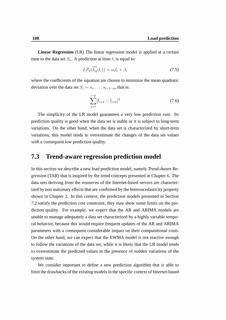
108 Load prediction
Linear Regression(LR) The linear regression model is applied at a certain
time to the data setSn. A prediction at timeti is equal to:
LPk(−→Lq(ti)) = αili + βi (7.5)
where the coefficients of the equation are chosen to minimizethe mean quadratic
deviation over the data setSi = si, . . . , si−1−n, that is:
i−p∑
j=i
[li+k − li+k]2 (7.6)
The simplicity of the LR model guarantees a very low prediction cost. Its
prediction quality is good when the data set is stable or it issubject to long-term
variations. On the other hand, when the data set is characterized by short-term
variations, this model tends to overestimate the changes ofthe data set values
with a consequent low prediction quality.
7.3 Trend-aware regression prediction model
In this section we describe a new load prediction model, namely Trend-Aware Re-
gression(TAR) that is inspired by the trend concepts presented in Chapter 6. The
data sets deriving from the resources of the Internet-basedservers are character-
ized by non stationary effects that are confirmed by the heteroscedasticity property
shown in Chapter 2. In this context, the prediction models presented in Section
7.2 satisfy the prediction cost constraint, they may show some limits on the pre-
diction quality. For example, we expect that the AR and ARIMAmodels are
unable to manage adequately a data set characterized by a highly variable tempo-
ral behavior, because this would require frequent updates of the AR and ARIMA
parameters with a consequent considerable impact on their computational costs.
On the other hand, we can expect that the EWMA model is not reactive enough
to follow the variations of the data set, while it is likely that the LR model tends
to overestimate the predicted values in the presence of sudden variations of the
system state.
We consider important to define a new prediction algorithm that is able to
limit the drawbacks of the existing models in the specific context of Internet-based

7.3 Trend-aware regression prediction model 109
systems. We think that the complexity of this context requires ameta-modelthat
can improve the prediction quality by gathering the best properties from the other
prediction algorithms still satisfying the constraints due to the prediction cost. An
ideal prediction model should combine the simplicity of theLR model, the AR and
ARIMA qualities of reproducing the stochastic pattern of the data set, the EWMA
ability of smoothing possible false predictions caused by some noise components.
To these purposes, a valid prediction algorithm should not consider just the data
set values or its predicted values, but it should also take into account the behavioral
trendof the system state deriving from the load trackers data set−→Lq(ti). The load
trend can give information about the behavior of the observed resource in the
past load representations (increasing, decreasing, oscillating, stabilizing). For this
reason, a trend-aware model cannot work on the observed dataset, but on a filtered
data set that excludes noise, and on the consequent estimation of the load trend.
This view should improve the prediction quality even when the system and the
observed data set are subject to a noisy signal. There are several possible models
that can satisfy a similar requirements. In this thesis, we propose a new linear
prediction algorithm, namely Trend-Aware Regression algorithm, that bases its
prediction model on the resource state representation and on its behavioral trend
as follows.
Let us considerm values selected with a constant frequencyΠ = n/m in the
so called history vector that is a subset of the data set−→Lq(ti). Between every pair
of consecutive points in the vector of−→Lq
Π(ti) = (li−jΠ), 0 ≤ j ≤ m, we compute
thetrend coefficientαi−jΠ of the line that divides the consecutive pointsli−jΠ and
li−(j+1)Π. In Figure 7.4, we show the trend coefficients when the history vector is
composed bym = 4 values. In order to quantify the trend value that is useful to
estimate the future valueli+k, we consider the weighted linear regression of them
trend coefficients:
αi−jΠ =li−jΠ − li−(j+1)Π
ti−jΠ − ti−(j+1)Π
; 0 ≤ j ≤ m − 1 (7.7)
αi =
m−1∑
j=0
pjαi−jΠ;
m−1∑
j=0
pj = 1 (7.8)
whereαi, . . . , αi−(m−1)Π are the trend coefficients weighted by them coefficients.
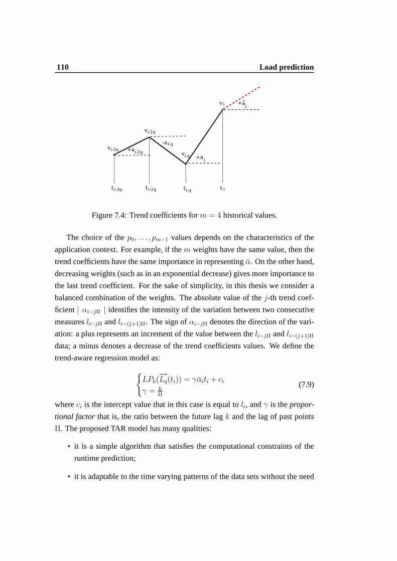
110 Load prediction
Figure 7.4: Trend coefficients form = 4 historical values.
The choice of thep0, . . . , pm−1 values depends on the characteristics of the
application context. For example, if them weights have the same value, then the
trend coefficients have the same importance in representingα. On the other hand,
decreasing weights (such as in an exponential decrease) gives more importance to
the last trend coefficient. For the sake of simplicity, in this thesis we consider a
balanced combination of the weights. The absolute value of the j-th trend coef-
ficient | αi−jΠ | identifies the intensity of the variation between two consecutive
measuresli−jΠ andli−(j+1)Π. The sign ofαi−jΠ denotes the direction of the vari-
ation: a plus represents an increment of the value between the li−jΠ andli−(j+1)Π
data; a minus denotes a decrease of the trend coefficients values. We define the
trend-aware regression model as:
{
LPk(−→Lq(ti)) = γαiti + ci
γ = kΠ
(7.9)
whereci is the intercept value that in this case is equal toli, andγ is thepropor-
tional factor that is, the ratio between the future lagk and the lag of past points
Π. The proposed TAR model has many qualities:
• it is a simple algorithm that satisfies the computational constraints of the
runtime prediction;
• it is adaptable to the time varying patterns of the data setswithout the need

7.4 Results 111
for a continuous and costly re-evaluation of the model parameters;
• it is able to reproduce the patterns of the data sets that allows it to be re-
sponsive to the load variations.
The TAR model can be considered as a meta-model from which it is possible
to obtain the other linear AR, EWMA and LR models. For example, the AR model
requiresp coefficients that are the firstp values of the auto-correlation function.
Consequently, to get AR from the TAR model we consider the number of trend
coefficientsm = n, the number of historical pointsn = p andφi−j as the ACF
values at timeti−j for 0 ≤ j ≤ n − 1. We can obtain the AR(p) model by setting
thepj coefficients of the Equation 7.8 to:
φi−jli−j(li−j − li−(j+1))
kti; 0 ≤ j ≤ n − 1 (7.10)
and the intercept valueci to ǫi. Similarly, to obtain an EWMA model from Equa-
tion 7.2, we can setci = αli andp0 equal to
αli(li − li−1)
kti(7.11)
whereα is the smoothing factor of the EWMA model.
7.4 Results
In this section we evaluate the predictability and the prediction window of the con-
sidered data sets and the quality of five runtime prediction models: AR, ARIMA,
EWMA, LR, TAR.
7.4.1 Predictability
The first step for efficacious prediction algorithms is the knowledge of the data
sets properties. We know that the observed data set of an Internet-based system are
completely unpredictable due to the high frequency component that perturbs the
signal. However, the filtering phase achieved through the load tracker functions
improves their predictability. In order to evaluate the prediction windowk, it is
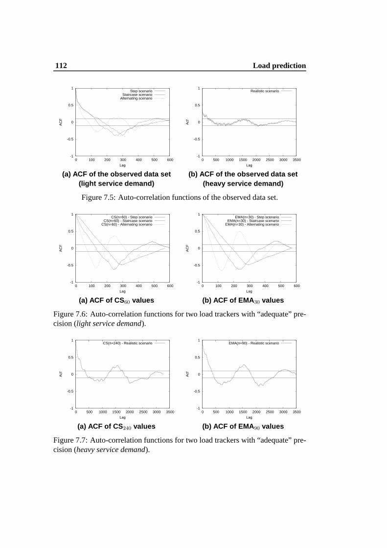
112 Load prediction
-1
-0.5
0
0.5
1
0 100 200 300 400 500 600
AC
F
Lag
Step scenarioStaircase scenario
Alternating scenario
(a) ACF of the observed data set(light service demand)
-1
-0.5
0
0.5
1
0 500 1000 1500 2000 2500 3000 3500
Acf
Lag
Realistic scenario
(b) ACF of the observed data set(heavy service demand)
Figure 7.5: Auto-correlation functions of the observed data set.
-1
-0.5
0
0.5
1
0 100 200 300 400 500 600
AC
F
Lag
CS(n=60) - Step scenarioCS(n=60) - Staircase scenario
CS(n=60) - Alternating scenario
(a) ACF of CS 60 values
-1
-0.5
0
0.5
1
0 100 200 300 400 500 600
AC
F
Lag
EMA(n=30) - Step scenarioEMA(n=30) - Staircase scenario
EMA(n=30) - Alternating scenario
(b) ACF of EMA 30 values
Figure 7.6: Auto-correlation functions for two load trackers with “adequate” pre-cision (light service demand).
-1
-0.5
0
0.5
1
0 500 1000 1500 2000 2500 3000 3500
Acf
Lag
CS(n=240) - Realistic scenario
(a) ACF of CS 240 values
-1
-0.5
0
0.5
1
0 500 1000 1500 2000 2500 3000 3500
Acf
Lag
EMA(n=90) - Realistic scenario
(b) ACF of EMA 90 values
Figure 7.7: Auto-correlation functions for two load trackers with “adequate” pre-cision (heavy service demand).
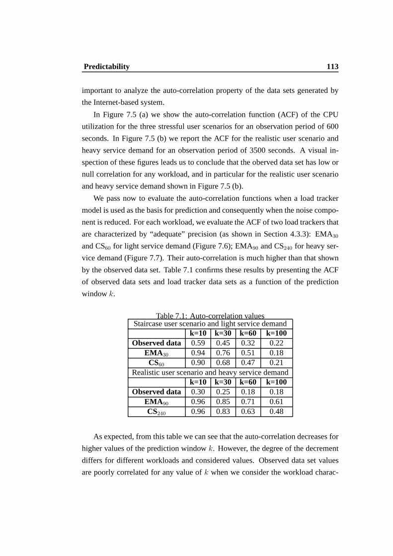
Predictability 113
important to analyze the auto-correlation property of the data sets generated by
the Internet-based system.
In Figure 7.5 (a) we show the auto-correlation function (ACF) of the CPU
utilization for the three stressful user scenarios for an observation period of 600
seconds. In Figure 7.5 (b) we report the ACF for the realisticuser scenario and
heavy service demand for an observation period of 3500 seconds. A visual in-
spection of these figures leads us to conclude that the oberved data set has low or
null correlation for any workload, and in particular for therealistic user scenario
and heavy service demand shown in Figure 7.5 (b).
We pass now to evaluate the auto-correlation functions whena load tracker
model is used as the basis for prediction and consequently when the noise compo-
nent is reduced. For each workload, we evaluate the ACF of twoload trackers that
are characterized by “adequate” precision (as shown in Section 4.3.3): EMA30
and CS60 for light service demand (Figure 7.6); EMA90 and CS240 for heavy ser-
vice demand (Figure 7.7). Their auto-correlation is much higher than that shown
by the observed data set. Table 7.1 confirms these results by presenting the ACF
of observed data sets and load tracker data sets as a functionof the prediction
windowk.
Table 7.1: Auto-correlation valuesStaircase user scenario and light service demand
k=10 k=30 k=60 k=100Observed data 0.59 0.45 0.32 0.22
EMA 30 0.94 0.76 0.51 0.18CS60 0.90 0.68 0.47 0.21
Realistic user scenario and heavy service demandk=10 k=30 k=60 k=100
Observed data 0.30 0.25 0.18 0.18EMA 90 0.96 0.85 0.71 0.61CS240 0.96 0.83 0.63 0.48
As expected, from this table we can see that the auto-correlation decreases for
higher values of the prediction windowk. However, the degree of the decrement
differs for different workloads and considered values. Observed data set values
are poorly correlated for any value ofk when we consider the workload charac-
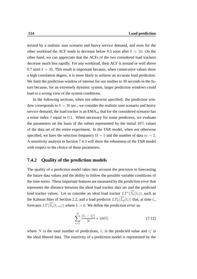
114 Load prediction
terized by a realistic user scenario and heavy service demand, and even for the
other workload the ACF tends to decrease below 0.5 soon afterk = 10. On the
other hand, we can appreciate that the ACFs of the two considered load trackers
decrease much less rapidly. For any workload, their ACF is around or well above
0.7 untilk = 30. This result is important because, when consecutive valuesshow
a high correlation degree, it is more likely to achieve an accurate load prediction.
We limit the prediction window of interest for our studies to30 seconds in the fu-
ture because, for an extremely dynamic system, larger prediction windows could
lead to a wrong view of the system conditions.
In the following sections, when not otherwise specified: theprediction win-
dow corresponds tok = 30 sec.; we consider the realistic user scenario and heavy
service demand; the load tracker is an EMA90 that for the considered scenario has
a noise indexδ equal to0.1. When necessary for some predictors, we evaluate
the parameters on the basis of the subset represented by the initial 10% values
of the data set of the entire experiment. In the TAR model, when not otherwise
specified, we have the selection frequencyΠ = 5 and the number of datam = 2.
A sensitivity analysis in Section 7.4.3 will show the robustness of the TAR model
with respect to the choice of these parameters.
7.4.2 Quality of the prediction models
The quality of a prediction model takes into account the precision in forecasting
the future data values and the ability to follow the possiblevariable conditions of
the time series. These important features are measured by theprediction errorthat
represents the distance between the ideal load tracker dataset and the predicted
load tracker values. Let us consider an ideal load trackerLT ∗(−→Sn(ti)), such as
the Kalman filter of Section 2.2, and a load predictorLPk(−→Lq(ti)) that, at timeti,
forecastsLT (−→Sn(ti+k)) wherek > 0. We define theprediction erroras:
N∑
i=1
|vi − v∗i |
N∗ 100% (7.12)
whereN is the total number of predictions,vi is the predicted value andv∗i is
the ideal filtered data. The reactivity of a prediction modelis represented by the
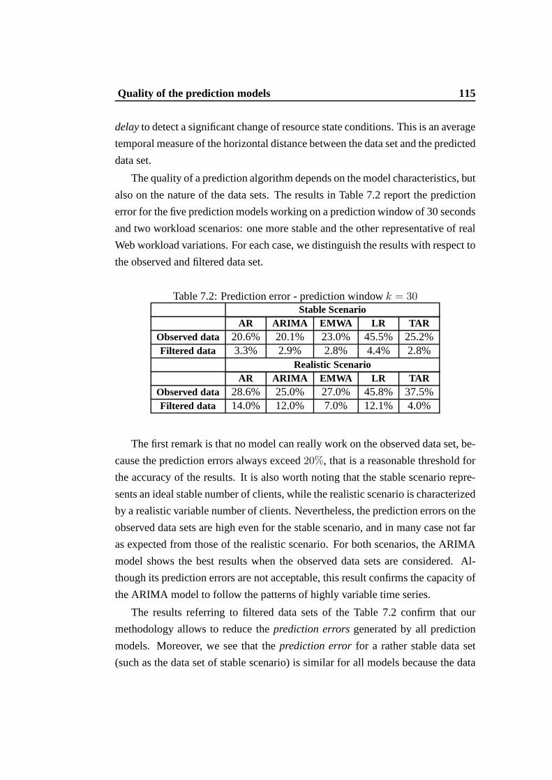
Quality of the prediction models 115
delayto detect a significant change of resource state conditions.This is an average
temporal measure of the horizontal distance between the data set and the predicted
data set.
The quality of a prediction algorithm depends on the model characteristics, but
also on the nature of the data sets. The results in Table 7.2 report the prediction
error for the five prediction models working on a prediction window of 30 seconds
and two workload scenarios: one more stable and the other representative of real
Web workload variations. For each case, we distinguish the results with respect to
the observed and filtered data set.
Table 7.2: Prediction error - prediction windowk = 30Stable Scenario
AR ARIMA EMWA LR TARObserved data 20.6% 20.1% 23.0% 45.5% 25.2%Filtered data 3.3% 2.9% 2.8% 4.4% 2.8%
Realistic ScenarioAR ARIMA EMWA LR TAR
Observed data 28.6% 25.0% 27.0% 45.8% 37.5%Filtered data 14.0% 12.0% 7.0% 12.1% 4.0%
The first remark is that no model can really work on the observed data set, be-
cause the prediction errors always exceed20%, that is a reasonable threshold for
the accuracy of the results. It is also worth noting that the stable scenario repre-
sents an ideal stable number of clients, while the realisticscenario is characterized
by a realistic variable number of clients. Nevertheless, the prediction errors on the
observed data sets are high even for the stable scenario, andin many case not far
as expected from those of the realistic scenario. For both scenarios, the ARIMA
model shows the best results when the observed data sets are considered. Al-
though its prediction errors are not acceptable, this result confirms the capacity of
the ARIMA model to follow the patterns of highly variable time series.
The results referring to filtered data sets of the Table 7.2 confirm that our
methodology allows to reduce theprediction errorsgenerated by all prediction
models. Moreover, we see that theprediction error for a rather stable data set
(such as the data set of stable scenario) is similar for all models because the data
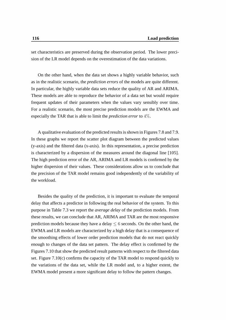
116 Load prediction
set characteristics are preserved during the observation period. The lower preci-
sion of the LR model depends on the overestimation of the datavariations.
On the other hand, when the data set shows a highly variable behavior, such
as in the realistic scenario, theprediction errorsof the models are quite different.
In particular, the highly variable data sets reduce the quality of AR and ARIMA.
These models are able to reproduce the behavior of a data set but would require
frequent updates of their parameters when the values vary sensibly over time.
For a realistic scenario, the most precise prediction models are the EWMA and
especially the TAR that is able to limit theprediction errorto 4%.
A qualitative evaluation of the predicted results is shown in Figures 7.8 and 7.9.
In these graphs we report the scatter plot diagram between the predicted values
(y-axis) and the filtered data (x-axis). In this representation, a precise prediction
is characterized by a dispersion of the measures around the diagonal line [105].
The high prediction error of the AR, ARIMA and LR models is confirmed by the
higher dispersion of their values. These considerations allow us to conclude that
the precision of the TAR model remains good independently ofthe variability of
the workload.
Besides the quality of the prediction, it is important to evaluate the temporal
delay that affects a predictor in following the real behavior of the system. To this
purpose in Table 7.3 we report theaverage delayof the prediction models. From
these results, we can conclude that AR, ARIMA and TAR are the most responsive
prediction models because they have a delay≤ 6 seconds. On the other hand, the
EWMA and LR models are characterized by a high delay that is a consequence of
the smoothing effects of lower order prediction models thatdo not react quickly
enough to changes of the data set pattern. The delay effect isconfirmed by the
Figures 7.10 that show the predicted result patterns with respect to the filtered data
set. Figure 7.10(c) confirms the capacity of the TAR model to respond quickly to
the variations of the data set, while the LR model and, to a higher extent, the
EWMA model present a more significant delay to follow the pattern changes.
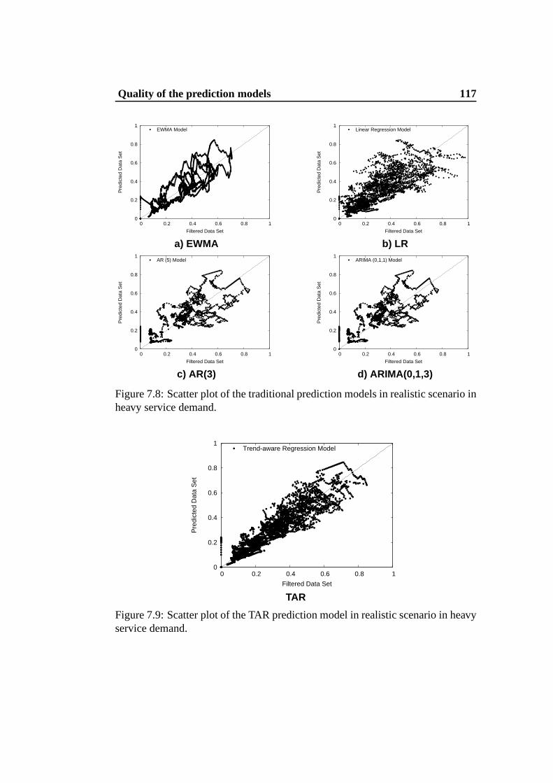
Quality of the prediction models 117
0
0.2
0.4
0.6
0.8
1
0 0.2 0.4 0.6 0.8 1
Pre
dict
ed D
ata
Set
Filtered Data Set
EWMA Model
a) EWMA
0
0.2
0.4
0.6
0.8
1
0 0.2 0.4 0.6 0.8 1
Pre
dict
ed D
ata
Set
Filtered Data Set
Linear Regression Model
b) LR
0
0.2
0.4
0.6
0.8
1
0 0.2 0.4 0.6 0.8 1
Pre
dict
ed D
ata
Set
Filtered Data Set
AR (5) Model
c) AR(3)
0
0.2
0.4
0.6
0.8
1
0 0.2 0.4 0.6 0.8 1
Pre
dict
ed D
ata
Set
Filtered Data Set
ARIMA (0,1,1) Model
d) ARIMA(0,1,3)
Figure 7.8: Scatter plot of the traditional prediction models in realistic scenario inheavy service demand.
0
0.2
0.4
0.6
0.8
1
0 0.2 0.4 0.6 0.8 1
Pre
dict
ed D
ata
Set
Filtered Data Set
Trend-aware Regression Model
TAR
Figure 7.9: Scatter plot of the TAR prediction model in realistic scenario in heavyservice demand.
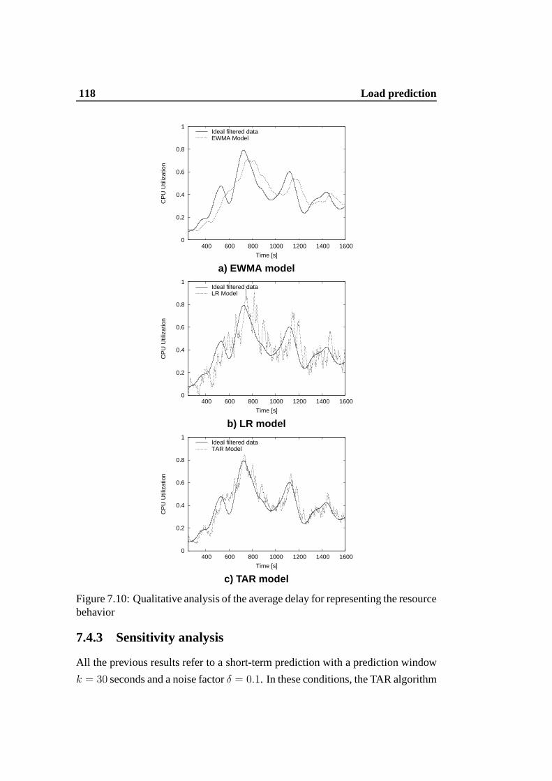
118 Load prediction
0
0.2
0.4
0.6
0.8
1
400 600 800 1000 1200 1400 1600
CP
U U
tiliz
atio
n
Time [s]
Ideal filtered dataEWMA Model
a) EWMA model
0
0.2
0.4
0.6
0.8
1
400 600 800 1000 1200 1400 1600
CP
U U
tiliz
atio
n
Time [s]
Ideal filtered dataLR Model
b) LR model
0
0.2
0.4
0.6
0.8
1
400 600 800 1000 1200 1400 1600
CP
U U
tiliz
atio
n
Time [s]
Ideal filtered dataTAR Model
c) TAR model
Figure 7.10: Qualitative analysis of the average delay for representing the resourcebehavior
7.4.3 Sensitivity analysis
All the previous results refer to a short-term prediction with a prediction window
k = 30 seconds and a noise factorδ = 0.1. In these conditions, the TAR algorithm
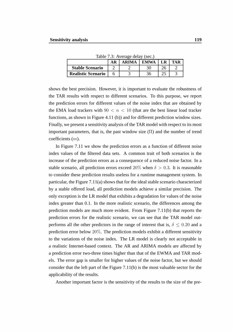
Sensitivity analysis 119
Table 7.3: Average delay (sec.)AR ARIMA EMWA LR TAR
Stable Scenario 2 2 30 26 2Realistic Scenario 6 3 36 25 3
shows the best precision. However, it is important to evaluate the robustness of
the TAR results with respect to different scenarios. To thispurpose, we report
the prediction errors for different values of the noise index that are obtained by
the EMA load trackers with90 < n < 10 (that are the best linear load tracker
functions, as shown in Figure 4.11 (b)) and for different prediction window sizes.
Finally, we present a sensitivity analysis of the TAR model with respect to its most
important parameters, that is, the past window size (Π) and the number of trend
coefficients (m).
In Figure 7.11 we show the prediction errors as a function of different noise
index values of the filtered data sets. A common trait of both scenarios is the
increase of the prediction errors as a consequence of a reduced noise factor. In a
stable scenario, all prediction errors exceed20% whenδ > 0.3. It is reasonable
to consider these prediction results useless for a runtime management system. In
particular, the Figure 7.11(a) shows that for the ideal stable scenario characterized
by a stable offered load, all prediction models achieve a similar precision. The
only exception is the LR model that exhibits a degradation for values of the noise
index greater than 0.1. In the more realistic scenario, the differences among the
prediction models are much more evident. From Figure 7.11(b) that reports the
prediction errors for the realistic scenario, we can see that the TAR model out-
performs all the other predictors in the range of interest that is, δ ≤ 0.20 and a
prediction error below20%. The prediction models exhibit a different sensitivity
to the variations of the noise index. The LR model is clearly not acceptable in
a realistic Internet-based context. The AR and ARIMA modelsare affected by
a prediction error two-three times higher than that of the EWMA and TAR mod-
els. The error gap is smaller for higher values of the noise factor, but we should
consider that the left part of the Figure 7.11(b) is the most valuable sector for the
applicability of the results.
Another important factor is the sensitivity of the results to the size of the pre-
120 Load prediction
diction windowk. We are in the context of runtime prediction in a short-term hori-
zon, hence we evaluate the prediction error fork ∈ [1, 120] seconds. Figure 7.12
reports the results for stable and realistic scenarios. In the former scenario, all
prediction models are valid and share similar behavior. In the latter more realistic
scenario, it is an important result that the error of the TAR model does not exceed
15% even fork = 120 seconds. The EWMA model shows close but slightly worse
results especially for lower values ofk; the LR model is not acceptable; even the
AR and ARIMA models must be discarded because of their doubled prediction
error, if compared to the TAR error.
All the previous results were achieved for fixed values of twoimportant pa-
rameters of the TAR algorithm. We now evaluate the sensitivity of the TAR model
with respect to the past valuesΠ and the number of trend coefficientsm. The re-
sults reported in Figure 7.13 are based on the ideal filtered data set and the filtered
data set with noise indexδ = 0.1. From this figure we can appreciate that the pre-
diction quality of the TAR model is preserved for a wide rangeof Π andm values
and for different filtered data sets. This robustness in a highly variable Internet-
based context is an important feature of the proposed model.No other prediction
algorithm guarantee similar stability.
7.5 Conclusions
This chapter has represented a first contribution in the direction of investigating
and predicting the performance of internal resources of Internet-based servers in
a short-term horizon.
We have evidenced that original observed data sets do not allow any predic-
tion, but the load trackers models reduce noises and exhibitrepresentations char-
acterized by some dependency that allows short-term prediction. However, some
popular runtime models that can be used for prediction produce unacceptable re-
sults even on filtered data set deriving from realistic workload scenarios. For this
reason, we have proposed a new prediction algorithm (Trend-Aware Regression
algorithm) that shows the best precision for different scenarios and stable results
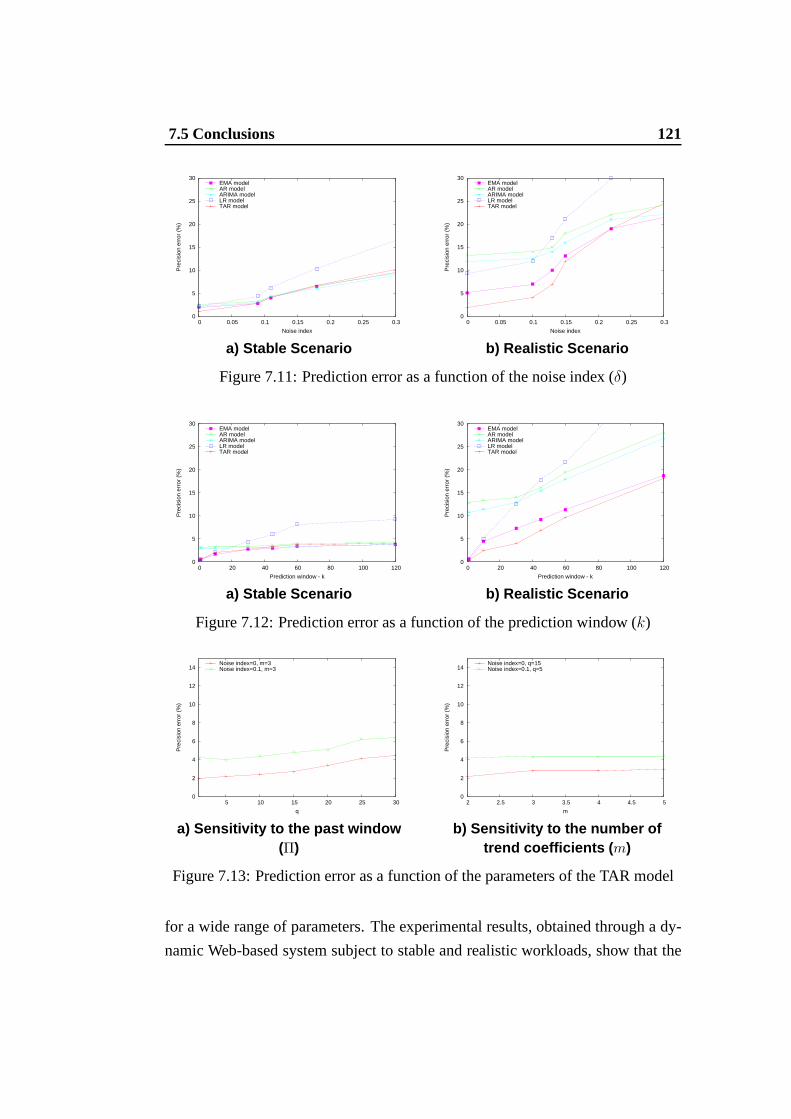
7.5 Conclusions 121
0
5
10
15
20
25
30
0 0.05 0.1 0.15 0.2 0.25 0.3
Pre
cisi
on e
rror
(%
)
Noise index
EMA modelAR modelARIMA modelLR modelTAR model
a) Stable Scenario
0
5
10
15
20
25
30
0 0.05 0.1 0.15 0.2 0.25 0.3
Pre
cisi
on e
rror
(%
)
Noise index
EMA modelAR modelARIMA modelLR modelTAR model
b) Realistic Scenario
Figure 7.11: Prediction error as a function of the noise index (δ)
0
5
10
15
20
25
30
0 20 40 60 80 100 120
Pre
cisi
on e
rror
(%
)
Prediction window - k
EMA modelAR modelARIMA modelLR modelTAR model
a) Stable Scenario
0
5
10
15
20
25
30
0 20 40 60 80 100 120
Pre
cisi
on e
rror
(%
)
Prediction window - k
EMA modelAR modelARIMA modelLR modelTAR model
b) Realistic Scenario
Figure 7.12: Prediction error as a function of the prediction window (k)
0
2
4
6
8
10
12
14
5 10 15 20 25 30
Pre
cisi
on e
rror
(%
)
q
Noise index=0, m=3Noise index=0.1, m=3
a) Sensitivity to the past window(Π)
0
2
4
6
8
10
12
14
2 2.5 3 3.5 4 4.5 5
Pre
cisi
on e
rror
(%
)
m
Noise index=0, q=15Noise index=0.1, q=5
b) Sensitivity to the number oftrend coefficients ( m)
Figure 7.13: Prediction error as a function of the parameters of the TAR model
for a wide range of parameters. The experimental results, obtained through a dy-
namic Web-based system subject to stable and realistic workloads, show that the

122 Load prediction
TAR algorithm satisfies the computational constraints of runtime prediction and
improves the accuracy of the prediction with respect to other algorithms based on
auto-regressive and linear models.

Chapter 8
Applications
In this Chapter, we validate the proposed multi-phase methodology by applying it
to support runtime management decisions in four Internet-based distributed sys-
tems 8.1. In the following sections we consider the following architectures:
• A quality guaranteedWeb cluster that requires a threshold-based admission
controller (Section 8.1);
• A locally distributed Network Intrusion Detection System (NIDS) that
is supported by a dynamic load balancer (Section 8.2);
• A geographically distributed system for content adaptationand deliv-
ery that implements the TAR prediction model for the load balancing (Sec-
tion 8.3);
• A multi-tier Web system that applies trend information algorithms for load
dispatching between the locally distributed servers (Section 8.4).
8.1 Web cluster
Several critical services are supported by Web clusters that are locally distributed
architectures characterized by multiple layers of servers. Two main problems af-
fect the quality of critical services [46]: overload risks when the volume of re-
quests temporarily exceed the capacity of the system, and slow response time
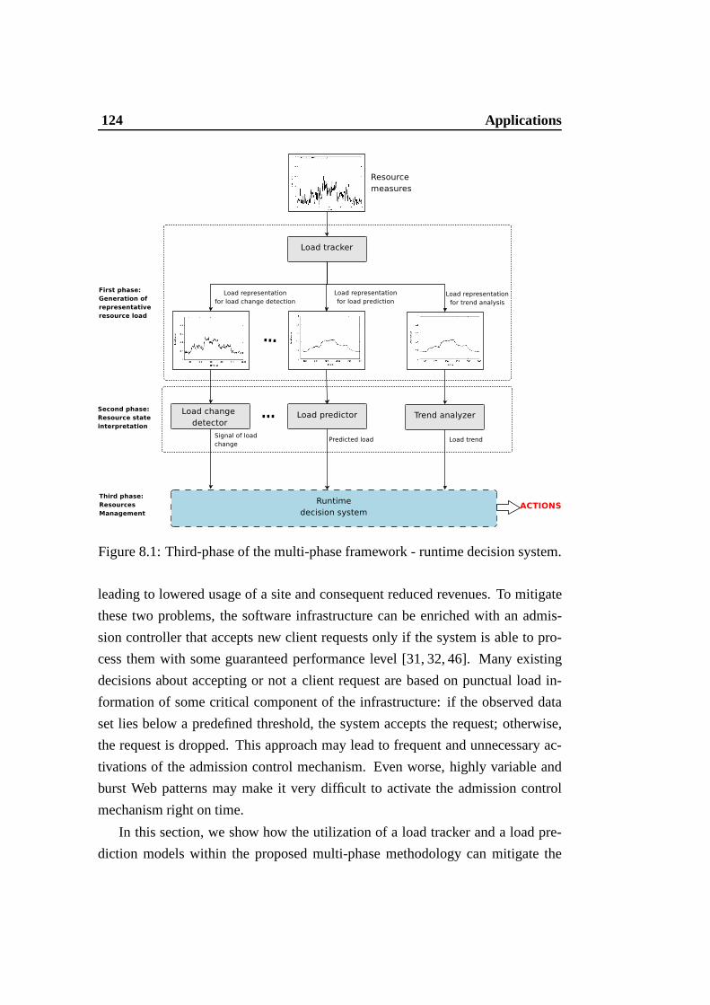
124 Applications
Figure 8.1: Third-phase of the multi-phase framework - runtime decision system.
leading to lowered usage of a site and consequent reduced revenues. To mitigate
these two problems, the software infrastructure can be enriched with an admis-
sion controller that accepts new client requests only if thesystem is able to pro-
cess them with some guaranteed performance level [31, 32, 46]. Many existing
decisions about accepting or not a client request are based on punctual load in-
formation of some critical component of the infrastructure: if the observed data
set lies below a predefined threshold, the system accepts therequest; otherwise,
the request is dropped. This approach may lead to frequent and unnecessary ac-
tivations of the admission control mechanism. Even worse, highly variable and
burst Web patterns may make it very difficult to activate the admission control
mechanism right on time.
In this section, we show how the utilization of a load trackerand a load pre-
diction models within the proposed multi-phase methodology can mitigate the
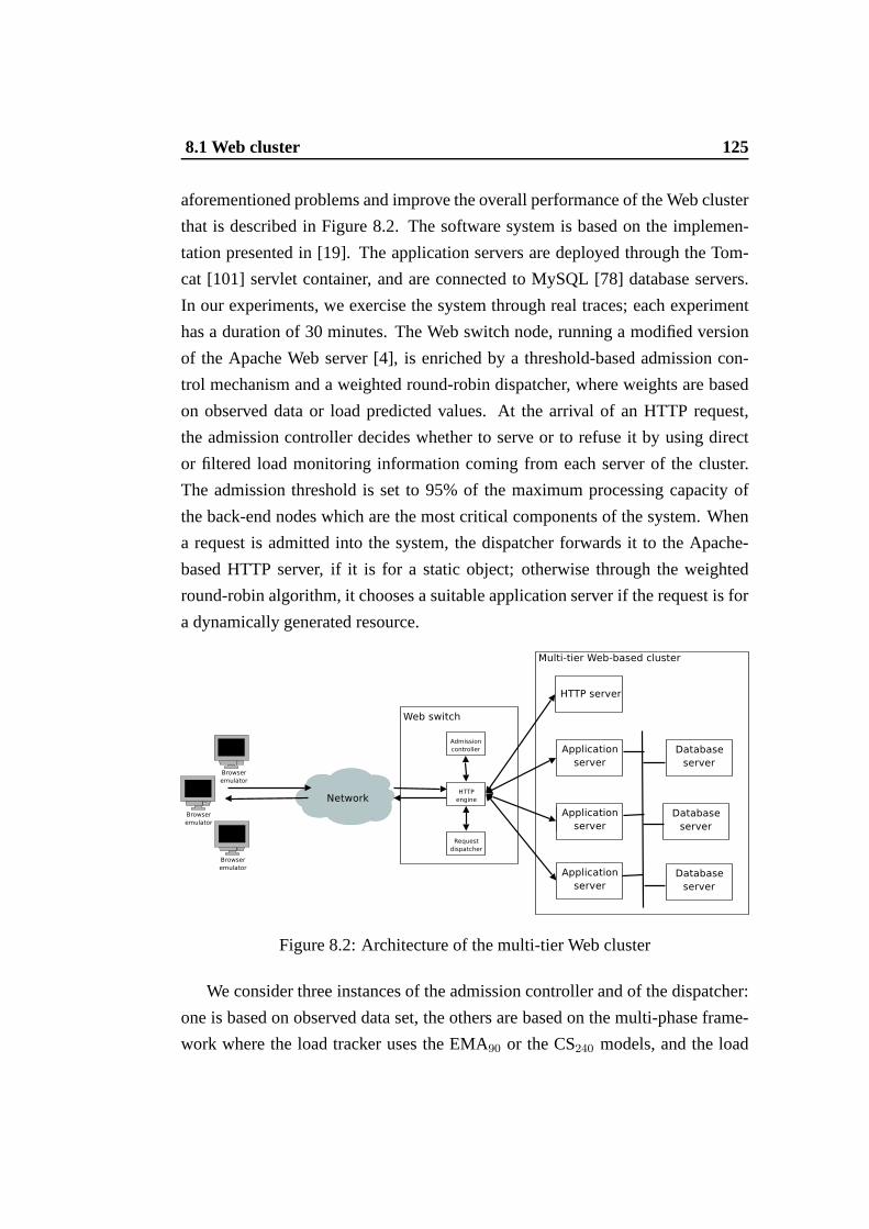
8.1 Web cluster 125
aforementioned problems and improve the overall performance of the Web cluster
that is described in Figure 8.2. The software system is basedon the implemen-
tation presented in [19]. The application servers are deployed through the Tom-
cat [101] servlet container, and are connected to MySQL [78]database servers.
In our experiments, we exercise the system through real traces; each experiment
has a duration of 30 minutes. The Web switch node, running a modified version
of the Apache Web server [4], is enriched by a threshold-based admission con-
trol mechanism and a weighted round-robin dispatcher, where weights are based
on observed data or load predicted values. At the arrival of an HTTP request,
the admission controller decides whether to serve or to refuse it by using direct
or filtered load monitoring information coming from each server of the cluster.
The admission threshold is set to 95% of the maximum processing capacity of
the back-end nodes which are the most critical components ofthe system. When
a request is admitted into the system, the dispatcher forwards it to the Apache-
based HTTP server, if it is for a static object; otherwise through the weighted
round-robin algorithm, it chooses a suitable application server if the request is for
a dynamically generated resource.
Figure 8.2: Architecture of the multi-tier Web cluster
We consider three instances of the admission controller andof the dispatcher:
one is based on observed data set, the others are based on the multi-phase frame-
work where the load tracker uses the EMA90 or the CS240 models, and the load

126 Applications
prediction is based on the TAR model of Section 7.3 where the parameters are
chosen asΠ = 5, m = 2 andk = 10. The activities of these three instances of
the admission control mechanism in terms of refused requests are shown in Fig-
ure 8.3. From this figure, we can observe that the use of the multi-phase method-
ology tends to reduce the number of unnecessary activationsof the admission
control mechanism, which are due to transient load spikes. Consequently, this
scheme allows the system to reject a minor number of requests. However, there
is a visual evidence that the EMA and CS load trackers have different effects that
we motivate below.
Table 8.1 summarizes the quantitative results of this case study. The first im-
portant result is that the multi-phase framework does not penalize the overall per-
formance of the system. Even if it accepts a much larger quantity of requests,
the impact on the 90-percentile of the response time is not perceived by a user.
Moreover, the use of the multi-phase methodology reduces some (unnecessary)
activations of the refusal mechanism, and limits the numberof refusals. These
positive effects are due to the combined benefits of the dispatching algorithm and
of the admission control mechanism based on predicted values.
From Figure 8.3 and Table 8.1, we can also conclude that the prediction based
on an EMA load tracker supports admission control algorithms more efficiently
than the CS-based alternative. This is in complete accordance with the results
shown in Section 4.3.3, where the precision affecting the CS240 load tracker was
significantly lower than that characterizing the EMA90 load tracker.
Table 8.1: Evaluation of the two admission control mechanisms90-Percentile Percentage Activations
of the Web page of refused of the admissionresponse time requests refusal
Observed data 3.08s 31% 140Multi-phase framework - EMA 90 3.71s 10% 35Multi-phase framework - CS240 3.26s 17.34% 72
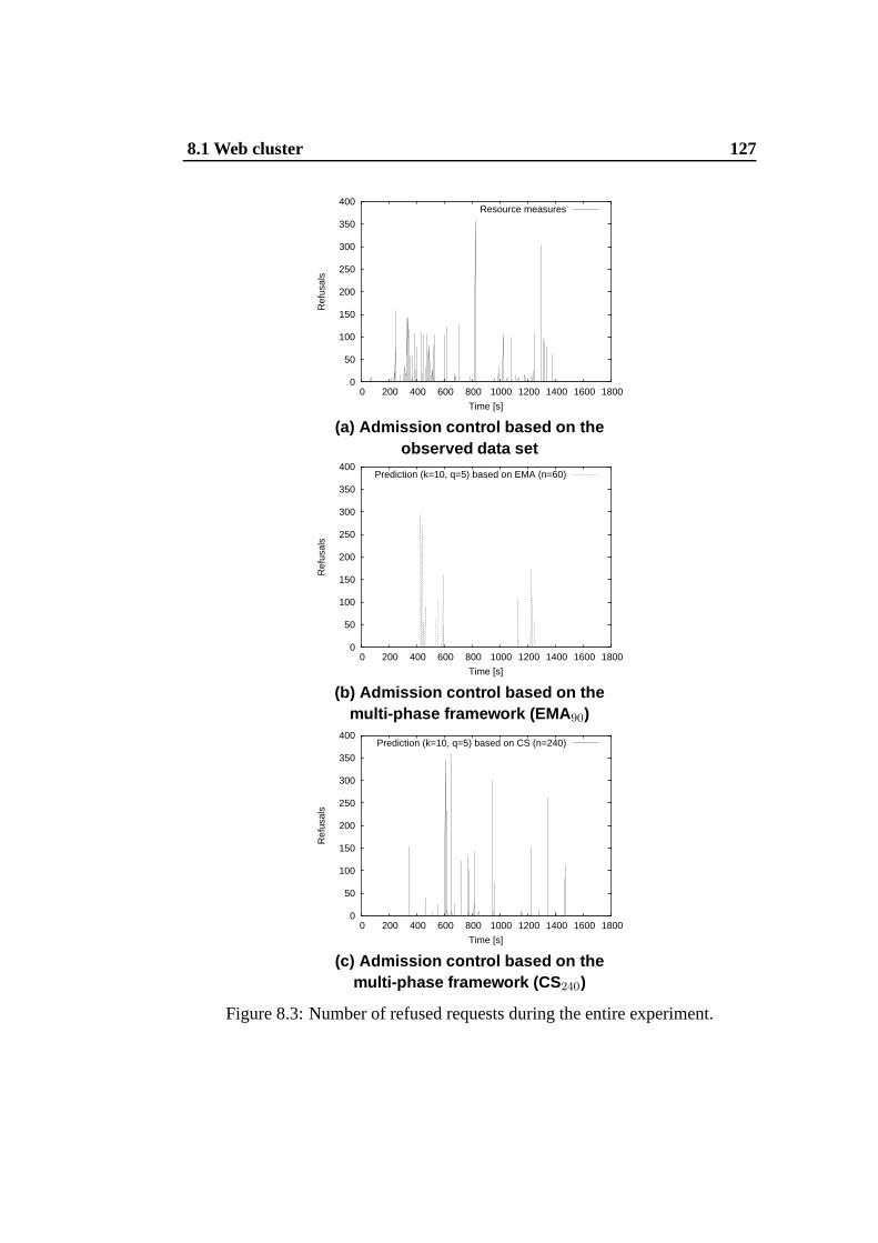
8.1 Web cluster 127
0
50
100
150
200
250
300
350
400
0 200 400 600 800 1000 1200 1400 1600 1800
Ref
usal
s
Time [s]
Resource measures
(a) Admission control based on theobserved data set
0
50
100
150
200
250
300
350
400
0 200 400 600 800 1000 1200 1400 1600 1800
Ref
usal
s
Time [s]
Prediction (k=10, q=5) based on EMA (n=60)
(b) Admission control based on themulti-phase framework (EMA 90)
0
50
100
150
200
250
300
350
400
0 200 400 600 800 1000 1200 1400 1600 1800
Ref
usal
s
Time [s]
Prediction (k=10, q=5) based on CS (n=240)
(c) Admission control based on themulti-phase framework (CS 240)
Figure 8.3: Number of refused requests during the entire experiment.
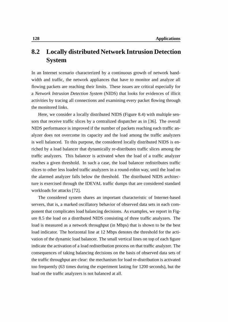
128 Applications
8.2 Locally distributed Network Intrusion DetectionSystem
In an Internet scenario characterized by a continuous growth of network band-
width and traffic, the network appliances that have to monitor and analyze all
flowing packets are reaching their limits. These issues are critical especially for
a Network Intrusion Detection System(NIDS) that looks for evidences of illicit
activities by tracing all connections and examining every packet flowing through
the monitored links.
Here, we consider a locally distributed NIDS (Figure 8.4) with multiple sen-
sors that receive traffic slices by a centralized dispatcheras in [36]. The overall
NIDS performance is improved if the number of packets reaching each traffic an-
alyzer does not overcome its capacity and the load among the traffic analyzers
is well balanced. To this purpose, the considered locally distributed NIDS is en-
riched by a load balancer that dynamically re-distributes traffic slices among the
traffic analyzers. This balancer is activated when the load of a traffic analyzer
reaches a given threshold. In such a case, the load balancer redistributes traffic
slices to other less loaded traffic analyzers in a round-robin way, until the load on
the alarmed analyzer falls below the threshold. The distributed NIDS architec-
ture is exercised through the IDEVAL traffic dumps that are considered standard
workloads for attacks [72].
The considered system shares an important characteristic of Internet-based
servers, that is, a marked oscillatory behavior of observeddata sets in each com-
ponent that complicates load balancing decisions. As examples, we report in Fig-
ure 8.5 the load on a distributed NIDS consisting of three traffic analyzers. The
load is measured as a network throughput (in Mbps) that is shown to be the best
load indicator. The horizontal line at 12 Mbps denotes the threshold for the acti-
vation of the dynamic load balancer. The small vertical lines on top of each figure
indicate the activation of a load redistribution process onthat traffic analyzer. The
consequences of taking balancing decisions on the basis of observed data sets of
the traffic throughput are clear: the mechanism for load re-distribution is activated
too frequently (63 times during the experiment lasting for 1200 seconds), but the
load on the traffic analyzers is not balanced at all.
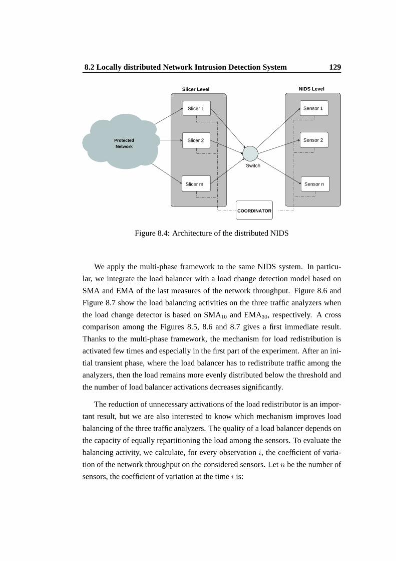
8.2 Locally distributed Network Intrusion Detection System 129
Slicer m
Slicer 2
Slicer 1 Sensor 1
Sensor n
Sensor 2
COORDINATOR
Slicer Level NIDS Level
ProtectedNetwork
Switch
Figure 8.4: Architecture of the distributed NIDS
We apply the multi-phase framework to the same NIDS system. In particu-
lar, we integrate the load balancer with a load change detection model based on
SMA and EMA of the last measures of the network throughput. Figure 8.6 and
Figure 8.7 show the load balancing activities on the three traffic analyzers when
the load change detector is based on SMA10 and EMA30, respectively. A cross
comparison among the Figures 8.5, 8.6 and 8.7 gives a first immediate result.
Thanks to the multi-phase framework, the mechanism for loadredistribution is
activated few times and especially in the first part of the experiment. After an ini-
tial transient phase, where the load balancer has to redistribute traffic among the
analyzers, then the load remains more evenly distributed below the threshold and
the number of load balancer activations decreases significantly.
The reduction of unnecessary activations of the load redistributor is an impor-
tant result, but we are also interested to know which mechanism improves load
balancing of the three traffic analyzers. The quality of a load balancer depends on
the capacity of equally repartitioning the load among the sensors. To evaluate the
balancing activity, we calculate, for every observationi, the coefficient of varia-
tion of the network throughput on the considered sensors. Let n be the number of
sensors, the coefficient of variation at the timei is:
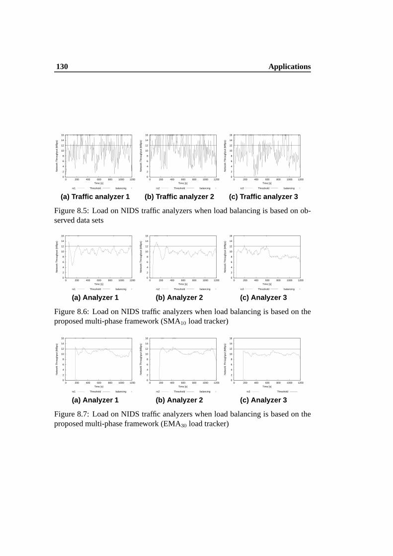
130 Applications
0
2
4
6
8
10
12
14
16
0 200 400 600 800 1000 1200
Net
wor
k T
hrou
ghpu
t (M
Bps
)
Time [s]
rs1 Threshold balancing
(a) Traffic analyzer 1
0
2
4
6
8
10
12
14
16
0 200 400 600 800 1000 1200
Net
wor
k T
hrou
ghpu
t (M
Bps
)
Time [s]
rs2 Threshold balancing
(b) Traffic analyzer 2
0
2
4
6
8
10
12
14
16
0 200 400 600 800 1000 1200
Net
wor
k T
hrou
ghpu
t (M
Bps
)
Time [s]
rs3 Threshold balancing
(c) Traffic analyzer 3
Figure 8.5: Load on NIDS traffic analyzers when load balancing is based on ob-served data sets
0
2
4
6
8
10
12
14
16
0 200 400 600 800 1000 1200
Net
wor
k T
hrou
ghpu
t (M
Bps
)
Time [s]
rs1 Threshold balancing
(a) Analyzer 1
0
2
4
6
8
10
12
14
16
0 200 400 600 800 1000 1200
Net
wor
k T
hrou
ghpu
t (M
Bps
)
Time [s]
rs2 Threshold balancing
(b) Analyzer 2
0
2
4
6
8
10
12
14
16
0 200 400 600 800 1000 1200
Net
wor
k T
hrou
ghpu
t (M
Bps
)
Time [s]
rs3 Threshold balancing
(c) Analyzer 3
Figure 8.6: Load on NIDS traffic analyzers when load balancing is based on theproposed multi-phase framework (SMA10 load tracker)
0
2
4
6
8
10
12
14
16
0 200 400 600 800 1000 1200
Net
wor
k T
hrou
ghpu
t (M
Bps
)
Time [s]
rs1 Threshold balancing
(a) Analyzer 1
0
2
4
6
8
10
12
14
16
0 200 400 600 800 1000 1200
Net
wor
k T
hrou
ghpu
t (M
Bps
)
Time [s]
rs2 Threshold balancing
(b) Analyzer 2
0
2
4
6
8
10
12
14
16
0 200 400 600 800 1000 1200
Net
wor
k T
hrou
ghpu
t (M
Bps
)
Time [s]
rs3 Threshold
(c) Analyzer 3
Figure 8.7: Load on NIDS traffic analyzers when load balancing is based on theproposed multi-phase framework (EMA30 load tracker)
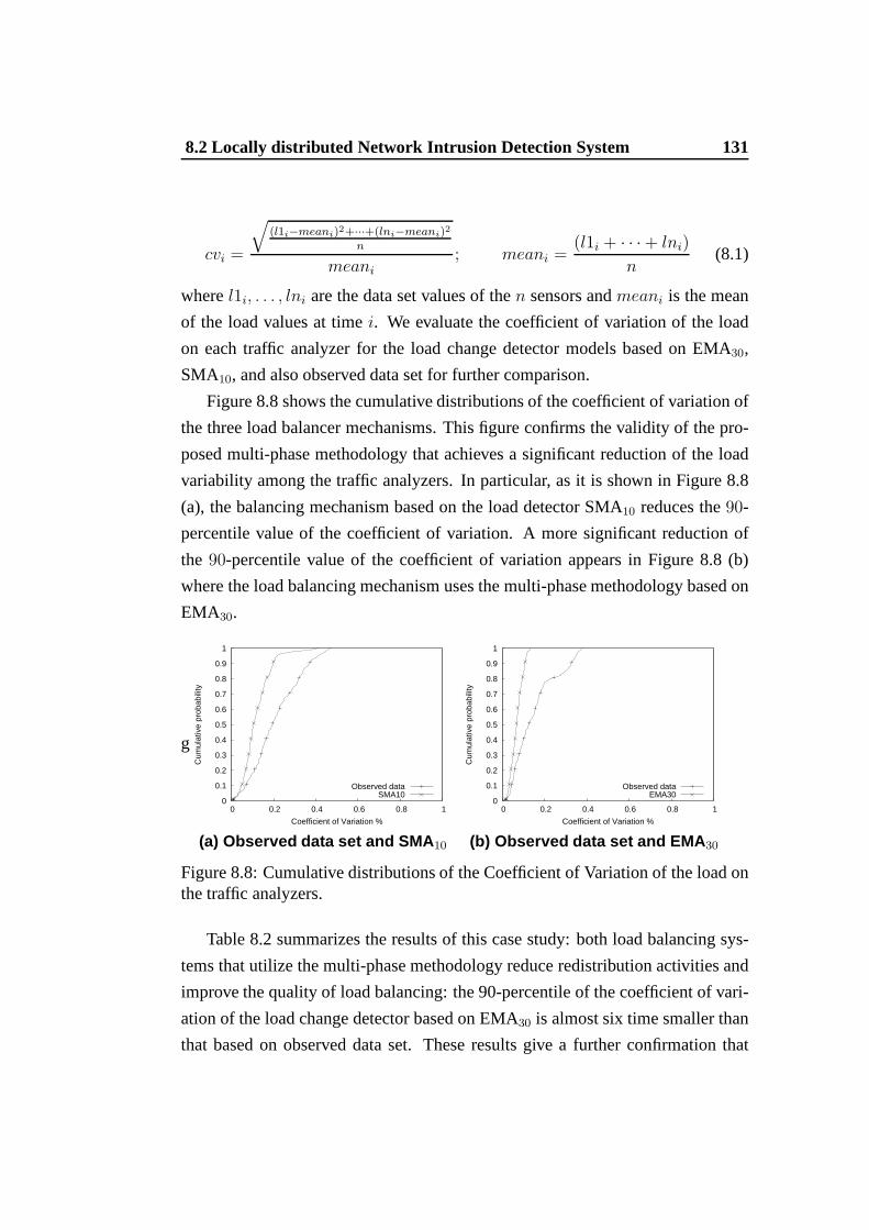
8.2 Locally distributed Network Intrusion Detection System 131
cvi =
√
(l1i−meani)2+···+(lni−meani)2
n
meani
; meani =(l1i + · · ·+ lni)
n(8.1)
wherel1i, . . . , lni are the data set values of then sensors andmeani is the mean
of the load values at timei. We evaluate the coefficient of variation of the load
on each traffic analyzer for the load change detector models based on EMA30,
SMA10, and also observed data set for further comparison.
Figure 8.8 shows the cumulative distributions of the coefficient of variation of
the three load balancer mechanisms. This figure confirms the validity of the pro-
posed multi-phase methodology that achieves a significant reduction of the load
variability among the traffic analyzers. In particular, as it is shown in Figure 8.8
(a), the balancing mechanism based on the load detector SMA10 reduces the90-
percentile value of the coefficient of variation. A more significant reduction of
the 90-percentile value of the coefficient of variation appears inFigure 8.8 (b)
where the load balancing mechanism uses the multi-phase methodology based on
EMA30.
g
0
0.1
0.2
0.3
0.4
0.5
0.6
0.7
0.8
0.9
1
0 0.2 0.4 0.6 0.8 1
Cum
ulat
ive
prob
abili
ty
Coefficient of Variation %
Observed dataSMA10
(a) Observed data set and SMA 10
0
0.1
0.2
0.3
0.4
0.5
0.6
0.7
0.8
0.9
1
0 0.2 0.4 0.6 0.8 1
Cum
ulat
ive
prob
abili
ty
Coefficient of Variation %
Observed dataEMA30
(b) Observed data set and EMA 30
Figure 8.8: Cumulative distributions of the Coefficient of Variation of the load onthe traffic analyzers.
Table 8.2 summarizes the results of this case study: both load balancing sys-
tems that utilize the multi-phase methodology reduce redistribution activities and
improve the quality of load balancing: the 90-percentile ofthe coefficient of vari-
ation of the load change detector based on EMA30 is almost six time smaller than
that based on observed data set. These results give a furtherconfirmation that

132 Applications
most of the redistributions carried out by the scheme based on observed data set
were not only useless, but had also a negative impact on load balancing.
Table 8.2: Evaluation of load balancing mechanisms90-percentile of the Total number of
Coefficient of Variation load re-distributionsActivation based on observed data 0.58 63
Activation based on SMA10 0.20 12Activation based on EMA30 0.10 13
8.3 Geographically distributed Web-based system
Many systems supporting popular Web-based services are based on architectures
that are distributed over a geographical scale. Here, we consider the problem of
delivering original and adaptive resources to heterogeneous client devices. When
the expected number of requests from heterogeneous classesof users and client
devices is high, a valid solution is to recur to a system consisting of a set of
centralized core nodes that are integrated with a set of geographically replicated
edge nodes [35], as shown in Figure 8.9. The edge nodes represent the front-
end part receiving all client requests. Each node is supported by a dispatching
mechanism that must decide at runtime which components of the Web resources
must be generated or adapted by the core nodes and which by theedge nodes.
Let us consider a popular mapping algorithm, such as the Weighted Round Robin
(WRR) [57], that takes its decisions depending on a dynamically evaluated weight
parameter. As most content adaptation services are CPU intensive tasks [27], this
weight is typically computed on the basis of the last value ofthe measured CPU
utilization (or the average of the last observed data) of thecore and edge nodes.
On the other hand, we suggest to use the multi-phase methodology to have a WRR
based on expected weights. In particular, we show that the proposed trend-aware
predictor (TAR) can improve the system performance substantially.
As the testbed for the experiments, we consider a distributed architecture con-
sisting of 20 physical servers, where 8 servers compose the core system and 12
servers are used for the edge nodes. The core system includes2 HTTP servers,
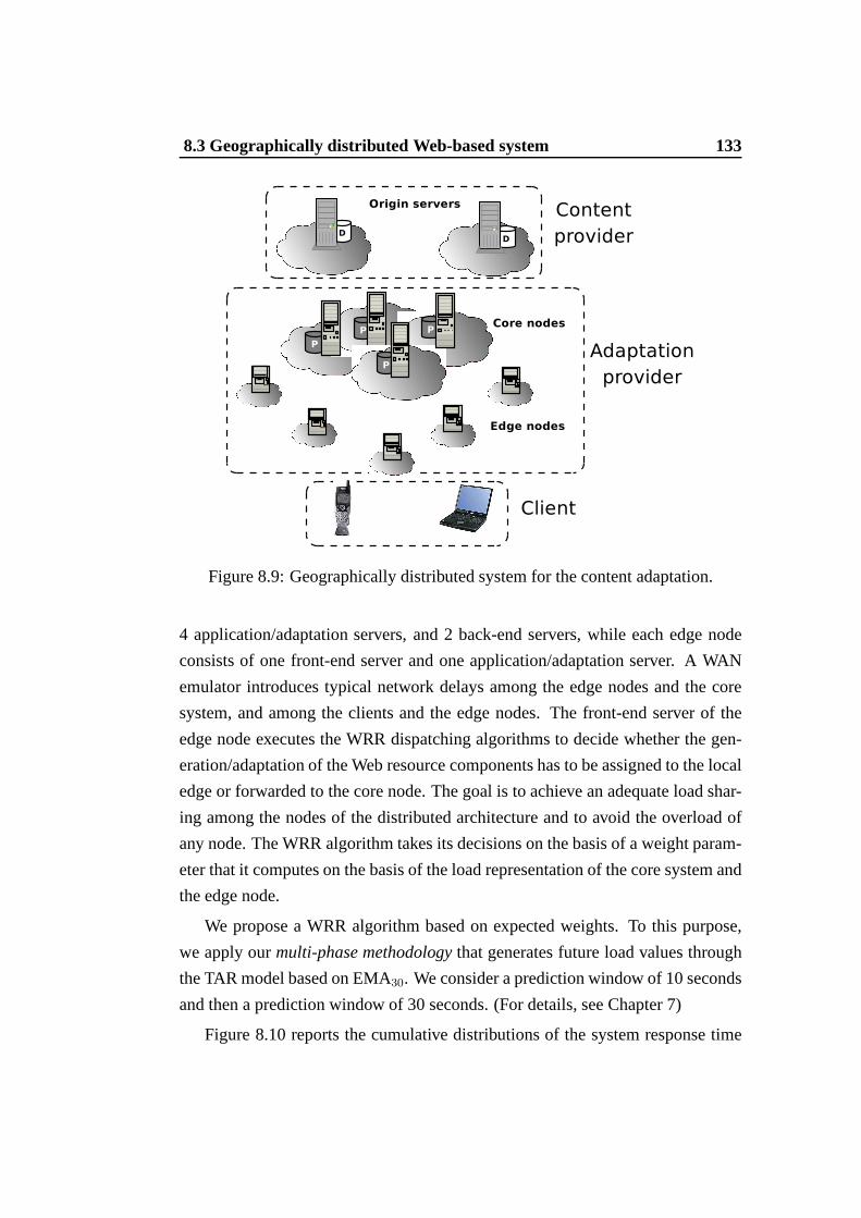
8.3 Geographically distributed Web-based system 133
Figure 8.9: Geographically distributed system for the content adaptation.
4 application/adaptation servers, and 2 back-end servers,while each edge node
consists of one front-end server and one application/adaptation server. A WAN
emulator introduces typical network delays among the edge nodes and the core
system, and among the clients and the edge nodes. The front-end server of the
edge node executes the WRR dispatching algorithms to decidewhether the gen-
eration/adaptation of the Web resource components has to beassigned to the local
edge or forwarded to the core node. The goal is to achieve an adequate load shar-
ing among the nodes of the distributed architecture and to avoid the overload of
any node. The WRR algorithm takes its decisions on the basis of a weight param-
eter that it computes on the basis of the load representationof the core system and
the edge node.
We propose a WRR algorithm based on expected weights. To thispurpose,
we apply ourmulti-phase methodologythat generates future load values through
the TAR model based on EMA30. We consider a prediction window of 10 seconds
and then a prediction window of 30 seconds. (For details, seeChapter 7)
Figure 8.10 reports the cumulative distributions of the system response time
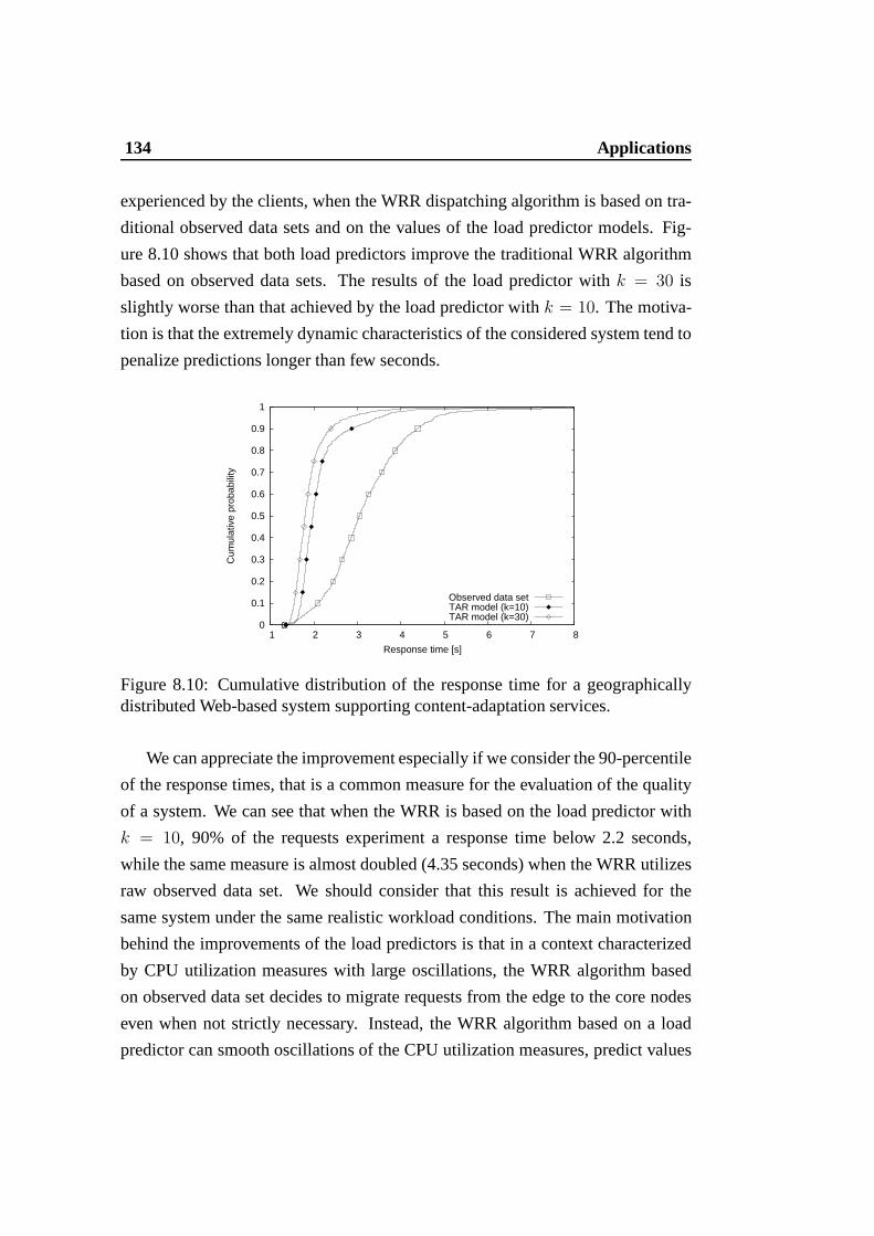
134 Applications
experienced by the clients, when the WRR dispatching algorithm is based on tra-
ditional observed data sets and on the values of the load predictor models. Fig-
ure 8.10 shows that both load predictors improve the traditional WRR algorithm
based on observed data sets. The results of the load predictor with k = 30 is
slightly worse than that achieved by the load predictor withk = 10. The motiva-
tion is that the extremely dynamic characteristics of the considered system tend to
penalize predictions longer than few seconds.
0
0.1
0.2
0.3
0.4
0.5
0.6
0.7
0.8
0.9
1
1 2 3 4 5 6 7 8
Cum
ulat
ive
prob
abili
ty
Response time [s]
Observed data setTAR model (k=10)TAR model (k=30)
Figure 8.10: Cumulative distribution of the response time for a geographicallydistributed Web-based system supporting content-adaptation services.
We can appreciate the improvement especially if we considerthe 90-percentile
of the response times, that is a common measure for the evaluation of the quality
of a system. We can see that when the WRR is based on the load predictor with
k = 10, 90% of the requests experiment a response time below 2.2 seconds,
while the same measure is almost doubled (4.35 seconds) whenthe WRR utilizes
raw observed data set. We should consider that this result isachieved for the
same system under the same realistic workload conditions. The main motivation
behind the improvements of the load predictors is that in a context characterized
by CPU utilization measures with large oscillations, the WRR algorithm based
on observed data set decides to migrate requests from the edge to the core nodes
even when not strictly necessary. Instead, the WRR algorithm based on a load
predictor can smooth oscillations of the CPU utilization measures, predict values
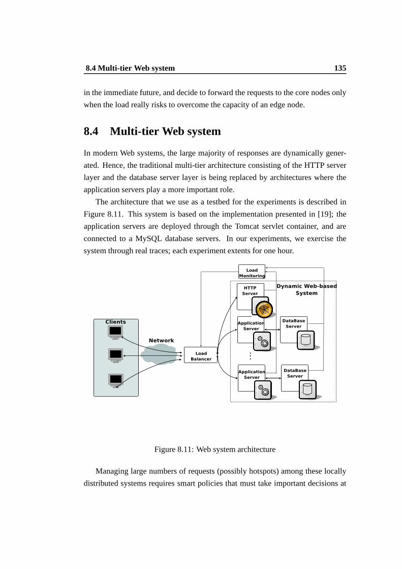
8.4 Multi-tier Web system 135
in the immediate future, and decide to forward the requests to the core nodes only
when the load really risks to overcome the capacity of an edgenode.
8.4 Multi-tier Web system
In modern Web systems, the large majority of responses are dynamically gener-
ated. Hence, the traditional multi-tier architecture consisting of the HTTP server
layer and the database server layer is being replaced by architectures where the
application servers play a more important role.
The architecture that we use as a testbed for the experimentsis described in
Figure 8.11. This system is based on the implementation presented in [19]; the
application servers are deployed through the Tomcat servlet container, and are
connected to a MySQL database servers. In our experiments, we exercise the
system through real traces; each experiment extents for onehour.
Figure 8.11: Web system architecture
Managing large numbers of requests (possibly hotspots) among these locally
distributed systems requires smart policies that must takeimportant decisions at
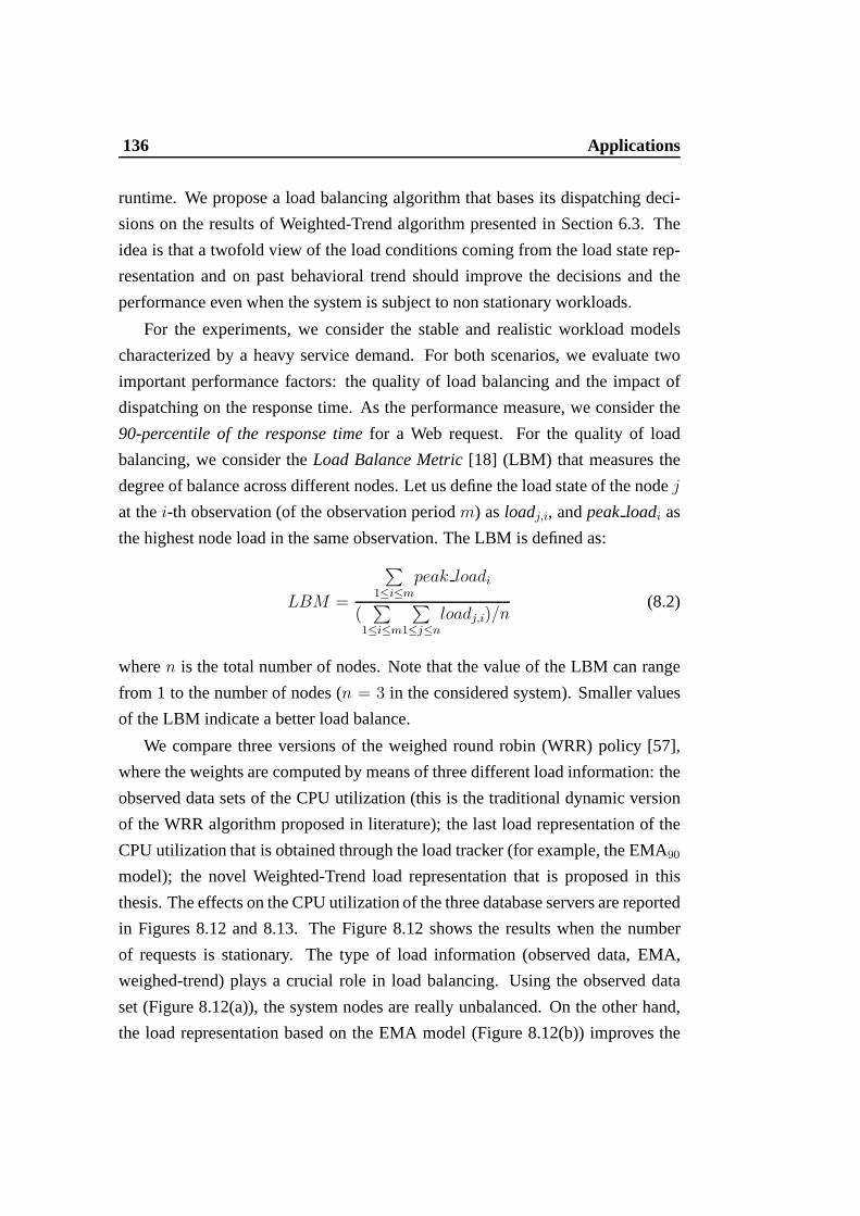
136 Applications
runtime. We propose a load balancing algorithm that bases its dispatching deci-
sions on the results of Weighted-Trend algorithm presentedin Section 6.3. The
idea is that a twofold view of the load conditions coming fromthe load state rep-
resentation and on past behavioral trend should improve thedecisions and the
performance even when the system is subject to non stationary workloads.
For the experiments, we consider the stable and realistic workload models
characterized by a heavy service demand. For both scenarios, we evaluate two
important performance factors: the quality of load balancing and the impact of
dispatching on the response time. As the performance measure, we consider the
90-percentile of the response timefor a Web request. For the quality of load
balancing, we consider theLoad Balance Metric[18] (LBM) that measures the
degree of balance across different nodes. Let us define the load state of the nodej
at thei-th observation (of the observation periodm) asloadj,i, andpeakloadi as
the highest node load in the same observation. The LBM is defined as:
LBM =
∑
1≤i≤m
peak loadi
(∑
1≤i≤m
∑
1≤j≤n
loadj,i)/n(8.2)
wheren is the total number of nodes. Note that the value of the LBM canrange
from 1 to the number of nodes (n = 3 in the considered system). Smaller values
of the LBM indicate a better load balance.
We compare three versions of the weighed round robin (WRR) policy [57],
where the weights are computed by means of three different load information: the
observed data sets of the CPU utilization (this is the traditional dynamic version
of the WRR algorithm proposed in literature); the last load representation of the
CPU utilization that is obtained through the load tracker (for example, the EMA90model); the novel Weighted-Trend load representation thatis proposed in this
thesis. The effects on the CPU utilization of the three database servers are reported
in Figures 8.12 and 8.13. The Figure 8.12 shows the results when the number
of requests is stationary. The type of load information (observed data, EMA,
weighed-trend) plays a crucial role in load balancing. Using the observed data
set (Figure 8.12(a)), the system nodes are really unbalanced. On the other hand,
the load representation based on the EMA model (Figure 8.12(b)) improves the
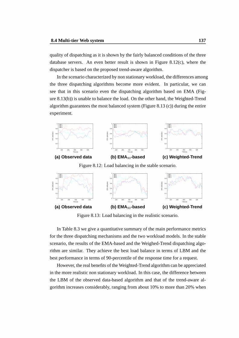
8.4 Multi-tier Web system 137
quality of dispatching as it is shown by the fairly balanced conditions of the three
database servers. An even better result is shown in Figure 8.12(c), where the
dispatcher is based on the proposed trend-aware algorithm.
In the scenario characterized by non stationary workload, the differences among
the three dispatching algorithms become more evident. In particular, we can
see that in this scenario even the dispatching algorithm based on EMA (Fig-
ure 8.13(b)) is unable to balance the load. On the other hand,the Weighted-Trend
algorithm guarantees the most balanced system (Figure 8.13(c)) during the entire
experiment.
0
0.2
0.4
0.6
0.8
1
100 200 300 400 500
CP
U u
tiliz
atio
n
Time [s]
DB 1DB 2DB 3
(a) Observed data
0
0.2
0.4
0.6
0.8
1
100 200 300 400 500
CP
U u
tiliz
atio
n
Time [s]
DB 1DB 2DB 3
(b) EMA90-based
0
0.2
0.4
0.6
0.8
1
100 200 300 400 500
CP
U u
tiliz
atio
n
Time [s]
DB 1DB 2DB 3
(c) Weighted-Trend
Figure 8.12: Load balancing in the stable scenario.
0
0.2
0.4
0.6
0.8
1
100 200 300 400 500
CP
U u
tiliz
atio
n
Time [s]
DB 1DB 2DB 3
(a) Observed data
0
0.2
0.4
0.6
0.8
1
100 200 300 400 500
CP
U u
tiliz
atio
n
Time [s]
DB 1DB 2DB 3
(b) EMA90-based
0
0.2
0.4
0.6
0.8
1
100 200 300 400 500
CP
U u
tiliz
atio
n
Time [s]
DB 1DB 2DB 3
(c) Weighted-Trend
Figure 8.13: Load balancing in the realistic scenario.
In Table 8.3 we give a quantitative summary of the main performance metrics
for the three dispatching mechanisms and the two workload models. In the stable
scenario, the results of the EMA-based and the Weighed-Trend dispatching algo-
rithm are similar. They achieve the best load balance in terms of LBM and the
best performance in terms of 90-percentile of the response time for a request.
However, the real benefits of the Weighted-Trend algorithm can be appreciated
in the more realistic non stationary workload. In this case,the difference between
the LBM of the observed data-based algorithm and that of the trend-aware al-
gorithm increases considerably, ranging from about 10% to more than 20% when
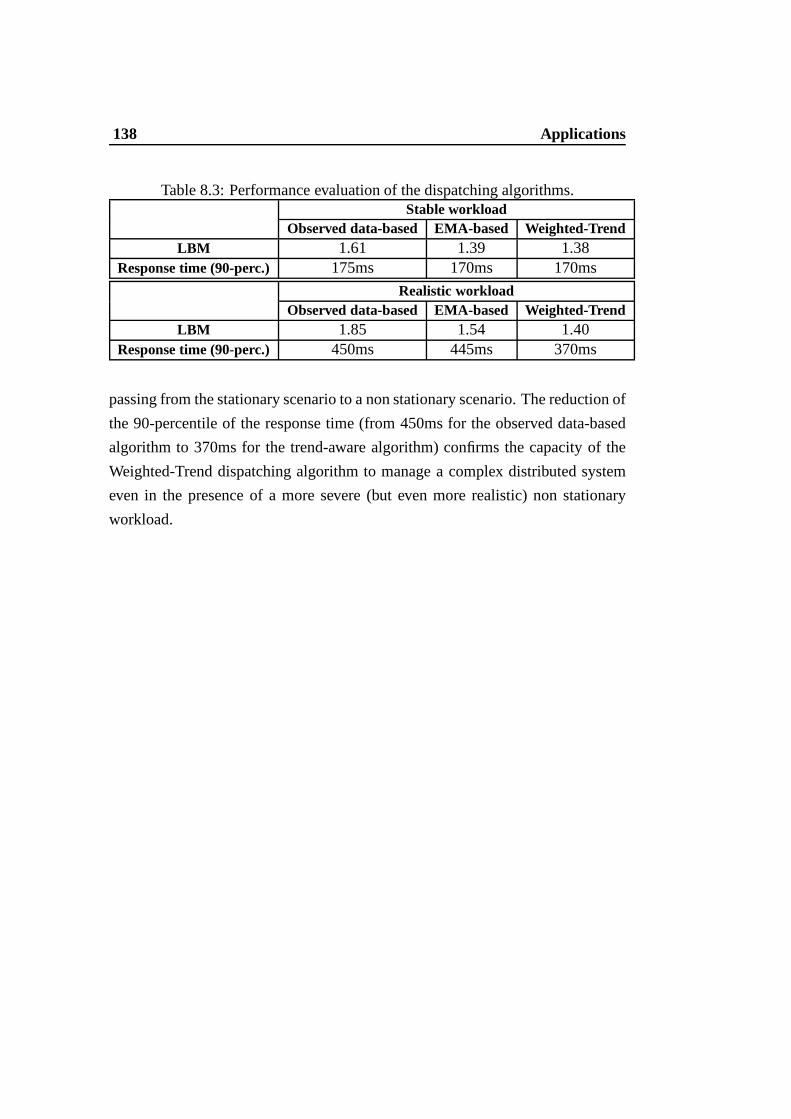
138 Applications
Table 8.3: Performance evaluation of the dispatching algorithms.Stable workload
Observed data-based EMA-based Weighted-TrendLBM 1.61 1.39 1.38
Response time (90-perc.) 175ms 170ms 170ms
Realistic workloadObserved data-based EMA-based Weighted-Trend
LBM 1.85 1.54 1.40Response time (90-perc.) 450ms 445ms 370ms
passing from the stationary scenario to a non stationary scenario. The reduction of
the 90-percentile of the response time (from 450ms for the observed data-based
algorithm to 370ms for the trend-aware algorithm) confirms the capacity of the
Weighted-Trend dispatching algorithm to manage a complex distributed system
even in the presence of a more severe (but even more realistic) non stationary
workload.
Chapter 9
Related work
The thesis has several innovative contributions that we distinguish in four main
areas.
• System view:internal vs. external;
• Data: observed resource measures vs. system load representationmodels;
• Context: realistic Internet-based systems vs. other distributed/parallel ap-
plications;
• Interpretation and decision algorithms: off-line vs. runtime schemes;
9.1 Internal vs. external system view
The workload characterization of Internet-based servers has received much atten-
tion for over a decade. Various metrics are collected, analyzed and visualized for
various reasons, such as traffic modeling, capacity planning and resource man-
agement. For example, the authors in [6] report a large set ofstatistics about
Web traffic (arrival pattern, request inter-arrival time and mix of requests), file
size and popularity, system performance in terms of response time and through-
put, typical client performance and user behavior. On the basis of these and other
statistics, several researchers have characterized the Web workload by fitting dis-
tributions to data (e.g., heavy-tailed distributions [5,8,28], burst arrivals [59] and
hot spots [10]) and by proposing performance models driven by such distribu-
tions [44].
140 Related work
All the analyses confirm that the external traffic reaching anInternet-based
system shows some periodic behavior [10] that facilitates its interpretation and
management. Hence, existing results are extremely useful for capacity planning
and system dimensioning goals, but they are useless to estimate a system state
at runtime. The main reason is that, as demonstrated in Chapter 2, the external
workload is not clearly correlated or completely uncorrelated with the internal
view of an Internet-based system. Consequently, an external view has little or no
possibility of really help a runtime management system to control the complexity
of modern processing schemes.
Even the most recent results oriented to the load state interpretations in the
presence of non stationary workloads [53, 61, 74, 92] are mainly focused to char-
acterize external factors, such as the arrival frequency. These measures can be
turned into some measure of the expected internal system load, but no result on
this topic exists, and even this thesis leaves this issue to future work.
Unlike all previous work on external analyses, we consider models and statis-
tics oriented to an original internal system view. In this context, we analyze the
performance indexes of the most critical internal system resources. This approach
motivates the necessity of the proposedmulti-phase methodology. Moreover, we
demonstrate that the stochastic characterization of the internal system states allow
us to support some important runtime decisions for distributed Internet-based sys-
tems, such as load sharing, load balancing, admission control, request redirection
even at a geographical scale.
Runtime load state interpretation of the internal resources has not received
much attention yet, especially if we refer to Internet-based systems. For exam-
ple, Pacifici et al. [79] propose a model for estimating at runtime the CPU de-
mand of Web applications, but not for positioning the systemstate with respect
to the resource capacities. Other studies that are orientedto an internal view do
not consider runtime constraints. Examples of them includeload balancer poli-
cies [2, 7, 17, 26, 48, 81], overload and admission controller schemes [81, 82],
request routing mechanisms and replica placement algorithms [63, 84, 94], dis-
tributed resource monitors [87].
9.2 Observed resource measures vs. load representation 141
9.2 Observed resource measures vs. load represen-tation
The detection of significant and permanent load changes of a system resource, the
prediction of the future load behavior and the definition of the trend of the past
load behavior are at the basis of most runtime management decisions of Internet-
based systems. All these tasks require information about the system state. For ex-
ample, taking autonomous decisions according to some objective rules for event
detection or for triggering actions concerning data/service placement but also to
detect overloaded or faulty components, requires the ability of automatically cap-
turing significant information about the internal state of the resources and also
adapting the monitoring system to internal and external conditions.
The common method to represent the resource state is based onthe periodic
collection of samples through server monitors and on the direct use of these val-
ues. Some low-pass filtering of network throughput samples has been proposed
in [90], but the large majority of resource state interpretation algorithms for the
runtime management of the Internet-based systems are basedon some functions
that work directly on resource measures [1,2,7,17,26,30,48,63,77,81,84,87,88,
94,111].
Even the studies based on a control theoretical approach to prevent overload
or to provide guaranteed levels of performance in Web systems [1, 60] refer to
direct resource measures (e.g., CPU utilization, average Web object response
time) as feedback signals. We have demonstrated that the problem with these
approaches is that most modern Internet-based systems are characterized by com-
plex hardware/software architectures and by highly variable workloads that cause
instability of system resource measures. Moreover, the observed measures of the
internal resources are characterized by some statistical properties, such as noise,
heteroscedasticity and short time dependency, that make the observed values com-
pletely unreliable for characterizing the system state with respect to the resource
capacities. The risk of extending the existing schemes to runtime management
decisions for Internet-based systems is to suggest completely wrong actions.
On the other hand, in our thesis we show that it is important ormandatory
to refer to stochastic representation models of the observed resource measures.
142 Related work
To this purpose, we refer also to the estimation theory. It support methodologies
for calculating usable approximations of data sets even if the input values are in-
complete, uncertain or noisy. In particular, the estimation theory assumes that the
desired information is embedded into a noisy signal. This theory is fundamental
for our purposes because we have demonstrated that the resource measures of an
Internet-based system are extremely noisy. Our preliminary experimental results
based on the estimation theory support the proposedmulti-phase methodologythat
first aims to represent the load behavior of an internal resource, and then uses this
load representation as the input for the state interpretation stochastic models such
as load change detectors, load prediction models and load trend schemes. These
models are really useful to support the most common runtime decision systems for
distributed Internet-based systems, such as admission control, load balancing and
request redirection. It is worth to observe that this is the first research that proposes
a thorough study and a general multi-phase methodology to support runtime de-
cisions in the context of adaptive and self-adaptive architectures and heavy-tailed
workloads characterizing modern Internet-based services. Moreover, the over-
all methodology is implemented and integrated into frameworks that have been
demonstrated to work well for different distributed Internet-based architectures.
9.3 Realistic Internet-based context
The thesis focuses on Internet-based systems characterized by sophisticated load
monitoring strategies and management tasks, and by heavy-tailed workloads that
are too complex for an analytical representation [49, 75]. Many previous studies
were oriented to simulation models of simplified Internet-based architectures [1,
24, 33, 81, 98]. Although the simulation of an Internet-based system is a chal-
lenging task by itself [50], the focus on real systems opens novel interesting and
challenging issues.
There are many studies on the characterization of resource loads, albeit related
to systems that are subject to workloads that are quite different from the load mod-
els considered in this thesis. Hence, many of the previous results cannot be applied
directly to the Internet-based systems considered here. For example, the authors
in [77] evaluate the effects of different load representations on job load balancing
9.4 Off-line models vs. runtime model 143
through a simulation model that assumes a Poisson job inter-arrival process. A
similar analysis concerning Unix systems is carried out in [48]. Dinda et al. [42]
investigate the predictability of the CPU load average in a Unix machine subject to
CPU bound jobs. The adaptive disk I/O prefetcher proposed in[103] is validated
through realistic disk I/O inter-arrival patterns referring to scientific applications.
The workload features considered in all these pioneer papers differ substantially
from the load models characterizing Internet-based servers that show high vari-
ability, bursty patterns and heavy-tails workload even at different time scales. The
are other works making strong assumptions on the nature of the workload, that
allow a simplification of many state interpretation problems. In particular, the
authors in [74] present a mechanism that works well with mildly oscillating or
stationary workloads; in [106] there are stochastic modelsfor the FTP transfer
times; in [42] there is an extensive study of the host CPU loadaverage; in [90]
there is some model on network traffic, which is assumed as a Gaussian process.
All these assumptions do not hold for the workloads characterizing Internet-based
systems that exhibit specific statistical properties.
Our research differs from previous works because it considers realistic work-
load scenarios. When you move from ideal to realistic workload conditions, al-
most all the considered stochastic models for the state representation and inter-
pretation exhibit high precision errors. On the other hand,the models proposed
in this thesis are demonstrated to work well even in conditions of real workload
Internet scenarios.
9.4 Off-line models vs. runtime model
A main difference of this thesis with respect to the literature is that the large
majority of decision systems that are necessary to support Internet-based services
have to satisfy runtime constraints while most of the existing interpretation and
decision models work off-line. Let us give some examples.
• Load representation.Many popular stochastic models for load representa-
tion are characterized by high overhead. This is the case of auto-regressive
integrated moving average (ARIMA) and auto-regressive fractionally inte-
144 Related work
grated moving average (ARFIMA) [42]. These models are able to reproduce
precisely the behavior of the data set, but at the price of high computational
cost and frequent updates of their parameters that are inadequate to the typ-
ical variability characterizing Internet-based systems.
• Load change detection. Many stochastic models for determining load
change detections are oriented to off-line schemes. The historical refer-
ence of all these studies is [80]. Subsequent investigations are in [55, 56,
68]. Other theoretical optimal results about the likelihood approach to load
change detection are proposed in [40]. It is impossible to propose a simple
application of these schemes to a runtime environment, although we could
extend some previous theoretical results, such as the CUSUMalgorithms,
to the load change detection problem in our contexts.
• Load prediction. There is a huge amount of prediction models that are ori-
ented to off-line studies. Just to give some examples, we cancite genetic
algorithms, support vector machines [37], machine learning techniques, and
Fuzzy systems [97]. None of them can be directly applied or adapted to sup-
port runtime predictions in a variable environment such as atypical Internet-
based system [41].
Even the most common methods for investigating the efficacy of load rep-
resentations for runtime management tasks work off-line. See for example the
models that analyze samples collected from access or resource usage logs [10,34,
42,64,71,90].
Hence, we can say that adequate models for supporting runtime management
decisions in highly variable systems represent open issues. One of the novel con-
tribution of the proposed methodology is to address some of these issues in the
context of adaptive Internet-based systems. The constraints due to runtime results
lead us to consider models that are characterized by low computational complex-
ity. For example, we consider many linear (e.g., the exponential moving average
of the CPU utilization [33]) and some non linear models (e.g., the cubic spline
functions in [47, 85, 110]) that may be used as a trend indicator in other contexts.
However, the authors in [33] limit their considerations only to a direct application
9.4 Off-line models vs. runtime model 145
of the exponential moving average model without any characterization of the data
set values that are used to generate the model. In our thesis,we carry out the first
sensitivity analysis of the models parameters and we validate the models through
different data sets.
For other problems, such as load prediction, the linear timeseries models [42,
71, 73, 90, 103] are not really suitable to face the characteristics and complex-
ity of highly variable workloads and Internet-based systems. In highly variable
and non stationary contexts, auto-regressive models such as AR and ARMA, re-
quire a continuous update of the parameters that is inappropriate to support most
runtime management decisions. Our results confirm that autoregressive models,
such as [60, 73], are useless when applied to highly variablecontexts. The mod-
els proposed in this thesis lack the learning capabilities and precision of other
more complex algorithms, but we should recall that in the considered context it
is mandatory to achieve good (not necessarily optimal) predictions quickly, rather
than looking for the optimal decision in an unpredictable amount of time. Our
runtime prediction models differ from previous results even because we do not
make any assumption (e.g., linearity, stability) on the distribution of the data set,
as required by other papers on runtime short-term predictions [42,74,90,106]. A
related linear prediction model is proposed by Squillante et al. [10], but it exhibits
a much lower precision than that characterizing our prediction algorithms.
If we pass to consider the last phase of the proposed methodology, we can
observe that runtime constraints are important requirements also for most deci-
sion systems. This is the case, for example, of admission control mechanisms,
replica placement policies, load balancing algorithms. For example, Cherkasova
et al. [33] validate their runtime session-based admissioncontroller for Web servers
through the SPECWeb96 workload [96], that nowadays is considered fairly ob-
solete [58, 95] with respect to the considered TPC-W workload [102] that is an
industrial standard benchmark for Web-based dynamic services. In [73, 88, 94],
the authors propose a simple and efficient methodology for a dynamic replica
placement and user request redirection. Other related runtime decision systems
are represented by the large literature on load balancing algorithms. We cite
few of them which are more closely related to distributed Internet-based sys-
tems [3,21,23,62,69,93]. This thesis is innovative with respect to these works be-

146 Related work
cause it is the first to apply stochastic models for load representation and runtime
decisions. Moreover, we propose also novel self-adaptive algorithm for geograph-
ically distributed systems. Other autonomic-like algorithms have been proposed
in quite different contexts [14, 54, 99, 112]. The proposal in [60] considers an al-
gorithm for a self-tuning admission controller in a locallydistributed system that
is similar to the multi-tier Web sites analyzed in this thesis.
Unlike all the previous literature that is oriented to specific applications, it is
worth to observe that our thesis proposes a first methodologythat is able to support
a large set of runtime decision algorithms specifically oriented to Internet-based
workload and adaptive Internet-based systems.
Chapter 10
Conclusions
This thesis addresses many important issues that are at the basis of runtime man-
agement decisions in Internet-based systems. To this purpose, we have first an-
alyzed the stochastic behavior of the internal resources measures of servers be-
longing to different Internet-based systems. Existing runtime management sys-
tems evaluate load conditions of system resources and then decide whether and
which action(s) it is important to carry out. We have shown that in the context of
Internet-based systems, characterized by highly variableworkload and complex
hardware/software architectures, it is inappropriate to take decisions on the basis
of rough system resource measures. The values obtained fromload monitors of
Internet-based servers offer an instantaneous view of the load conditions of a re-
source and they are of little help for understanding the realload trends and for
anticipating future load conditions. In fact, we have demonstrated that the statis-
tical properties of the system resource measures evidence avery low correlation
between the internal and the external system view, a high dispersion of the ob-
served values, a high noise component, a significant heteroscedastisity and a low
or null auto-correlation.
The results have motivated the proposal of an innovativemulti-phase method-
ologythat separates the complex problems behind runtime management decisions
in different processes. In particular, we first achieve a representative view of the
system state by adapting and proposing novel stochastic models that are charac-
terized by a computational complexity in accordance to the computational con-
straints of runtime decisions. Although the so calledload trackersallow us to
148 Conclusions
have manageable data sets, we have proved that some traditional model could be
inaccurate in the presence of non stationary and heteroscedastic workload condi-
tions. For this reason, we have proposed aself-adaptiveload tracker that selects
the parameters on the basis of the statistical properties ofthe observed data set,
such as the standard deviation. This class of load tracker improves the load tracker
qualities especially when the characteristics of the data set changes significantly
during the observation time.
We have applied these representative models to support fundamental tasks
characterizing runtime management decisions in Internet-based systems, such as
load change detection, load trend analysisand load predictionproblems. For
example, we have proved that through the load tracker functions the quality of
the load change detectors improves in terms of minimizing false detections. An-
other example is represented by the novel Trend-Aware Regression algorithm that
shows the best precision for different workload scenarios and robust results for a
wide range of parameters.
We have then proposed new runtime decision systems, which are based on
the best stochastic models, for some classic problems characterizing distributed
Internet-based systems, such as load balancing, admissioncontrol and requests
redirection. It is worth to note that all the phases of the multi-phase methodol-
ogy have been integrated into software modules of various prototypes consisting
of multiple Internet-based servers, such as a multi-tier Web system, a Web clus-
ter, a geographically distributed architecture and an Intrusion Detection System
for request dispatching, load balancing, admission control and request redirection
purposes and for a large set of representative workload models. In all contexts,
the achieved results are quite satisfactory. For these reasons, we think that the
proposed multi-phase methodology can be improved and extended to other prob-
lems. For the former goal, it would be important to study novel load tracker
functions that can integrate internal resource measures and external data referring
to the workload. We expect that in this way we could achieve even a more ro-
bust representation of the present and expected behavior ofcomplex distributed
systems. Positive results in this field would allow us to extend the proposed short
prediction models to medium- and probably long-term predictions even in highly
variable conditions. Another possible field of applicationof the proposed multi-

149
phase methodology is represented by the recentautonomic systemsthat are char-
acterized by several necessities of almost independent modules for self-inspection,
self-organization and self-configuration.

150 Conclusions
Bibliography
[1] T. Abdelzaher, K. G. Shin, and N. Bhatti. Performance guarantees for Webserver end-systems: A control-theoretical approach.IEEE Trans. Parallel andDistributed Systems, 13(1):80–96, Jan. 2002.
[2] M. Andreolini, M. Colajanni, and M. Nuccio. Scalabilityof content-aware serverswitches for cluster-based Web information systems. InProc. of WWW, Budapest,HU, May 2003.
[3] D. Andresen, T. Yang, and O. H. Ibarra. Towards a scalabledistributed WWWserver on networked workstations.J. of Parallel and Distributed Computing,42:91–100, 1997.
[4] Apache Server Foundation. Apache HTTP Server Project.http://www.apache.org.
[5] M. Arlitt, D. Krishnamurthy, and J. Rolia. Characterizing the scalability of a largeweb-based shopping system.IEEE Trans. Internet Technology, 1(1):44–69, Aug.2001.
[6] K. Arun, M. S. Squillante, L. Zhang, and J. Poirier. Analysis and characterizationof large-scale Web server access patterns and performance.World Wide Web, 2(1-2):85–100, Mar. 1999.
[7] J. Bahi, S. Contassot-Vivier, and R. Couturier. Dynamicload balancing and effi-cient load estimators for asynchronous iterative algorithms. IEEE Trans. Paralleland Distributed Systems, 16(4):289–299, Apr. 2006.
[8] P. Barford and M. E. Crovella. Generating representative Web workloads for net-work and server performance evaluation. InProc. of the Joint International Con-ference on Measurement and Modeling of Computer Systems (SIGMETRICS1998),Madison, WI, June 1998.
[9] M. I. Baron. Nonparametric adaptive change-point estimation and on-line detec-tion. Sequential Analysis, 19(1-2):1–23, 2000.
[10] Y. Baryshnikov, E. Coffman, G. Pierre, D. Rubenstein, M. Squillante, andT. Yimwadsana. Predictability of Web server traffic congestion. In Proc.of the 10th International Workshop on Web Content Caching and Distribution(WCW2005), Sophia Antipolis, FR, Sep. 2005.
[11] M. Basseville and I. Nikiforov.Detection of Abrupt Changes:Theory and Appli-cation. Prentice-Hall, 1993.
[12] M. Basseville and I. V. Nikiforov.Detection of Abrupt Changes:Theory and Ap-plication. Prentice-Hall.
152 BIBLIOGRAPHY
[13] D. Bonett. Approximate confidence interval for standard deviation of nonnormaldistributions. Computational Statistics and Data Analysis, 50(3):775–882, Feb.2006.
[14] D. Breitgand, E. Henis, and O. Shehory. Automated and adaptive threshold setting:enabling technology for autonomy and selfmanagement. InProc. of the Interna-tional Conference on Autonomic Computing (ICAC), 2005.
[15] T. Breusch and A. Pagan. ”a simple test for heteroscedasticity and random coeffi-cient variation”.Econometrica, 47:1287–129, 1979.
[16] B. L. Brockwell and R. A. Davis.Time Series: Theory and Methods. Springer-Verlag, 1987.
[17] H. Bryhni. A comparison of load balancing techniques for scalable web servers.IEEE Network, 14(4):58–64, July 2000.
[18] R. B. Bunt, D. L. Eager, G. M. Oster, and C. L. Williamson.Achieving loadbalance and effective caching in clustered Web servers. InProc. of WCW, SanDiego, CA, USA, USA, Apr. 1999.
[19] H. W. Cain, R. Rajwar, M. Marden, and M. H. Lipasti. An architectural evaluationof Java TPC-W. InProc. of the 7th Symposium on High Performance ComputerArchitecture (HPCA2001), Monterrey, ME, Jan. 2001.
[20] C. Canali and M. Rabinovich.Utility computing for Internet applications. Bookchapter in Web Content Delivery. Springer Verlag, NY, USA, 2004.
[21] V. Cardellini, E. Casalicchio, M. Colajanni, and P. Yu.The state of the art inlocally distributed Web-server system.ACM Computing Surveys, pages 263–311,2002.
[22] V. Cardellini, M. Colajanni, and P. Yu. Request redirection algorithms for dis-tributed Web systems.IEEE Trans. Parallel and Distributed Systems, 14(5):355–368, May 2003.
[23] V. Cardellini, M. Colajanni, and P. S. Yu. Redirection algorithms for load sharingin distributed Web-server systems. InProc. of IEEE 19th International Conf. onDistributed Computing Systems, Austin, TX, June 1999.
[24] V. Cardellini, M. Colajanni, and P. S. Yu. Geographic load balancing for scal-able distributed Web systems. InProc. of 8th International Workshop on Model-ing, Analysis, and Simulation of Computer and Telecommunication Systems (MAS-COTS 2000), San Francisco, CA, USA, Aug./Sept. 2000.
[25] T. Carozzi and A. Buckley. Deriving the sampling errorsof correlograms for gen-eral white noise.ArvXiv physics e-prints, May. 2005.
[26] M. Castro, M. Dwyer, and M. Rumsewicz. Load balancing and control for dis-tributed World Wide Web servers. InProceedings of the Intl. Conference on Con-trol Applications (CCA 1999), Kohala Coast, HI, Aug. 1999.
[27] E. Cecchet, A. Chanda, S. Elnikety, J. Marguerite, and W. Zwaenepoel. Perfor-mance comparison of middleware architectures for generating dynamic Web con-tent. InProc. of the 4th ACM/IFIP/USENIX Middleware Conference (MIDDLE-WARE2003), Rio de Janeiro, BR, June 2003.
BIBLIOGRAPHY 153
[28] J. Challenger, P. Dantzig, A. Iyengar, M. Squillante, and L. Zhang. Efficientlyserving dynamic data at highly accessed Web sites.IEEE/ACM Trans. on Net-working, 12(2):233–246, Apr. 2004.
[29] H. Chen and P. Mohapatra. Session-based overload control in qos-aware webservers. InProc. of the 21st Annual Joint Conference of the IEEE Computer andCommunications Societies (INFOCOM2002), New York, NY, June 2002.
[30] H. Chen and P. Mohapatra. Overload control in qos-awareweb servers.ComputerNetworks, 42(1):119–133, May 2003.
[31] X. Chen and J. Heidemann. Flash crowd mitigation via an adaptive admissioncontrol based on application-level measurement. Technical Report ISI-TR-557,USC/Information Sciences Institute, May 2002.
[32] L. Cherkasova and P. Phaal. Session based admission control: a mechanism forimproving performance of commercial Web sites. InProc. of the InternationalWorkshop on Quality of Service, London, June 1999.
[33] L. Cherkasova and P. Phaal. Session-based Admission Control: a Mechanismfor Peak Load Management of Commercial Web Sites.IEEE Trans. Computers,51(6):669–685, June 2002.
[34] B. Choi, J. Park, and Z. Zhang. Adaptive random samplingfor load change de-tection. InProc. of the 16th IEEE International Conference on Communications(ICC2003), Anchorage, AL, USA, May 2003.
[35] M. Colajanni, R. Lancellotti, and P. Yu. Distributed architectures for web contentadaptation and delivery. In S. Chanson and X. Tang, editors,Web Content Delivery.Springer, 2005.
[36] M. Colajanni and M. Marchetti. A parallel architecturefor stateful intrusion detec-tion in high traffic networks. InProc. of the IEEE/IST Workshop on Monitoring,Attack Detection and Mitigation (MonAM2006), Tuebingen, DE, Sept. 2006.
[37] C. Cortes and V. Vapnik. Support-vector networks.Machine Learning, 20(3),1995.
[38] M. E. Crovella, M. S. Taqqu, and A. Bestavros. Heavy-tailed probability distribu-tions in the World Wide Web. InA Practical Guide To Heavy Tails, pages 3–26.Chapman and Hall, New York, 1998.
[39] M. Dahlin. Interpreting stale load information.IEEE Trans. Parallel and Dis-tributed Systems, 11(10):1033–1047, Oct. 2000.
[40] J. Deshayes and P. D. Off-line statistical analysis of change-point models usingnon parametric and likelihood methods.In Detection of Abrupt Changes in Signalsand Dynamical Systems, pages 103–168, 1986.
[41] L. Devroye, L. Gyorfi, and G. Lugosi.A Probabilistic Theory of Pattern Recogni-tion. Springer-Verlag, 1996.
[42] P. Dinda and D. O’Hallaron. Host load prediction using linear models.ClusterComputing, 3(4):265–280, Dec. 2000.
[43] R. C. Dodge, D. A. Menasce, and D. Barbara. Testing e-commerce site scalabilitywith TPC-W . In Proc. of the 27th Computer Measurement Group Conference(CMG2001), Anaheim, CA, Dec. 2001.
154 BIBLIOGRAPHY
[44] A. B. Downey and D. G. Feitelson. The elusive goal of workload characterization.Performance Evaluation, 26(4):14–29, 1999.
[45] N. G. Duffield and F. Lo Presti. Multicast inference of packet delay variance atinterior network links. InProc. of the 19th IEEE Intl. Conference on ComputerCommunications (INFOCOM 2000), Tel Aviv, Israel, mar. 2000.
[46] S. Elnikety, E. Nahum, J. Tracey, and W. Zwaenepoel. A method for transparentadmission control and request scheduling in e-commerce Websites. InProc. ofthe 13th International World Wide Web Conference, New York, NY, 2004.
[47] R. L. Eubank and E. Eubank.Non parametric regression and spline smoothing.Marcel Dekker, 1999.
[48] D. Ferrari and S. Zhou. An empirical investigation of load indices for load balanc-ing applications. InProc. of the 12th IFIP International Symposium on ComputerPerformance, Modeling, Measurements and Evaluation (PERFORMANCE1987),Brussels, BE, Dec. 1987.
[49] G. Fishman and I. Adan. How heavy-tailed distributionsaffect simulation-generated time averages.ACM Trans. on Modeling and Computer Simulation,16(2):152–173, Apr. 2006.
[50] S. Floyd and V. Paxson. Difficulties in simulating the internet. IEEE/ACM Trans.Networking, 9(3):392–403, Aug. 2001.
[51] G. E. Forsythe, M. A. Malcolm, and C. B. Moler.Computer Methods for Mathe-matical Computations. Prentice-Hall, 1977.
[52] A. G. Ganek and T. Corbi. The dawning of the autonomic computing era. IBMSystems Journal, 42(1):5–18, Jan. 2003.
[53] D. Gmach, J. Rolia, L. Cherkasova, and A. Kemper. Capacity management anddemand prediction for next generation data centers. InProc. of the 5th IEEEInternational Conference on Web Services (ICWS2007), Salt Lake City, UT, July2007.
[54] J. R. Gruser, L. Raschid, V. Zadorozhny, and T. Zhan. Learning response timefor websources using query feedback and application in query optimization. TheInternational Journal on Very Large Data Bases, 9(1), Mar. 2000.
[55] D. V. Hinkley. Inference about the change point in a sequence of random variables.Biometrika, 57:1–17, 1970.
[56] D. V. Hinkley. Inference about the change point from cumulative sum-tests.Biometrika, 58:509–523, 1971.
[57] G. Hunt, G. Goldszmidt, R. King, and R. Mukherjee. Network web switch: Aconnection router for scalable internet services. InProc. of WWW, Brisbane, Aus-tralia, Apr. 1998.
[58] R. Iyer. Exploring the cache design space for Web servers. In Proc. of the 15thInt’l Parallel and Distributed Processing Symposium (PDPS2001), San Francisco,CA, USA, 2001.
[59] J. Jung, B. Krishnamurthy, and M. Rabinovich. Flash crowds and denial of serviceattacks: characterization and implications for CDNs and Web sites. InProc. ofthe 11th International World Wide Web Conference (WWW2002), Honolulu, HW,May 2002.
BIBLIOGRAPHY 155
[60] A. Kamra, V. Misra, and E. M. Nahum. Yaksha: a self-tuning controller for man-aging the performance of 3-tiered sites. InProc. of Twelfth International Workshopon Quality of Service (IWQOS2004), Montreal, CA, June 2004.
[61] N. Kandasamy, S. Abdelwahed, and J. P. Hayes. Self-optimization in computersystems via on-line control: application to power management. In Proc. of the 1stInternational Conference on Autonomic Computing (ICAC 2004), New York, NY,May 2004.
[62] J. Kangasharju, K. W. Ross, and J. W. Roberts. Performance evaluation of redi-rection schemes in content distribution networks. InComputer Communications,volume 24. Elsevier Science, Feb. 2001.
[63] P. Karbhari, M. Rabinovich, Z. Xiao, and F. Douglis. ACDN: a content deliv-ery network for applications. InProc. of 21st Int’l ACM SIGMOD Conference,Madison, WI, USA, 2002.
[64] T. Kelly. Detecting performance anomalies in global applications. InProc. of the2nd USENIX Workshop on Real, Large Distributed Systems (WORLDS2005), SanFrancisco, CA, USA, 2005.
[65] M. Kendall and J. Ord.Time Series. Oxford University Press, 1990.[66] J. F. Kenney and E. S. Keeping.Mathematics of Statistics. Van Nostrand, 1962.[67] J. O. Kephart and D. M. Chess. The vision of Autonomic Computing. IEEE
Computer, 36(1):41–50, Jan. 2003.[68] N. Kligiene and T. L. Methods of detecting instants of change of random process
properties.Automation and Remote Control, 44:1241–1283, 1983.[69] B. Krishnamurthy and J. Wang. On network-aware clustering of Web clients. In
Proc. of ACM Sigcomm 2000, Stockholm, Sweden, Aug. 2000.[70] D. J. Lilja. Measuring computer performance. A practitioner’s guide. Cambridge
University Press, 2000.[71] Y. Lingyun, I. Foster, and J. M. Schopf. Homeostatic andtendency-based CPU
load predictions. InProc. of the 17th Parallel and distributed processing Sympo-sium (IPDPS2003), Nice, FR, 2003.
[72] R. Lippmann, J. W. Haines, D. Fried, and K. Korba, J. Das.Analysis and results ofthe 1999 DARPA off-line intrusion detection evaluation. InProceedings of the 3rdIntl. Workshop on Recent Advances in Intrusion Detection (RAID 2000), London,UK, Oct. 2000.
[73] F. L. Lo Presti, N. Bartolini, and C. Petrioli. Dynamic replica placement and userrequest redirection in content delivery networks. InProceedings of the 11th IEEEIntl. Conference on Networks (ICON 2003), Sydeny, AUS, Oct. 2003.
[74] Y. Lu, T. Abdelzaher, L. Chenyang, S. Lui, and L. Xue. Feedback control withqueueing-theoretic prediction for relative delay guarantees in Web servers. InProc.of the 9th IEEE real-time and embedded technology and Applications Symposium(RTAS2003), Charlottesville, VA, May 2003.
[75] S. Luo and G. Marin. Realistic internet traffic simulation through mixture mod-eling and a case study. InProc. of the IEEE Winter Simulation Conference(WSC2005), Orlando, FL, USA, 2005.
156 BIBLIOGRAPHY
[76] D. Menasce and J. Kephart. Autonomic computing.IEEE Internet Computing,11(1):18–21, Jan. 2007.
[77] M. Mitzenmacher. How useful is old information.IEEE Trans. Parallel and Dis-tributed Systems, 11(1):6–20, Jan. 2000.
[78] MySQL database server, 2005. – http://www.mysql.com/.[79] G. Pacifici, W. Segmuller, M. Spreitzer, and A. Tantawi.Dynamic estimation
of CPU demand of Web traffic. InProc. of the 1st International Conference onPerformance Evaluation Methodologies and Tools (VALUETOOLS2006), Pisa, IT,Oct. 2006.
[80] E. S. Page. Estimating the point of change in a continuous process.Biometrika,44:248–252, 1957.
[81] V. S. Pai, M. Aron, G. Banga, M. Svendsen, P. Druschel, W.Zwaenepoel,and E. M. Nahum. Locality-aware request distribution in cluster-based networkservers. InProc. of the 8th International Conference on ArchitecturalSupport forProgramming Languages and Operating Systems (ASPLOS1998), San Jose, CA,Oct. 1998.
[82] R. Pandey and R. Barnes, J. F. Olsson. Supporting quality of service in HTTPservers. InProc. of the ACM Symposium on Principles of Distributed Computing,Puerto Vallarta, MX, June 1998.
[83] D. B. Percival and A. T. Walden.Wavelet Methods for Time Series Analysis. Cam-bridge University Press, 2000.
[84] G. Pierre and M. Van Steen. Globule: a platform for self replicating Webdocuments. InProc. of 6th Conference on protocols for Multimedia systems(PROMS2001), Enschede, NL, 2001.
[85] D. J. Poirier. Piecewise regression using cubic spline. Journal of the AmericanStatistical Association, 68(343):515–524, Sep. 1973.
[86] P. Pradhan, R. Tewari, S. Sahu, A. Chandra, and P. Shenoy. An observation-basedapproach towards self-managing web servers. InProc. of 10th International Work-shop on Quality of Service (IWQOS2002), Monterey, CA, USA, May 2002.
[87] M. Rabinovich, S. Triukose, Z. Wen, and L. Wang. DipZoom: the internetmeasurement marketplace. InProc. of 9th IEEE Global Internet Symposium,Barcelona, ES, 2006.
[88] M. Rabinovich, X. Zhen, and A. Aggarwal. Computing on the edge: a platformfor replicating internet applications. InProc. of 8th Int’l Workshop of Web ContentCaching and Distribution (WCW2003), Hawthorne, NY, USA, 2003.
[89] P. Ramanathan. Overload management in real-time control applications using(m,k)-firm guarantee.Performance Evaluation Review, 10(6):549–559, Jun. 1999.
[90] A. Sang and S. Li. A predictability analysis of network traffic. In Proc. of the 19thAnnual Joint Conference of the IEEE Computer and Communications Societies(INFOCOM2000), Tel Aviv, ISR, Mar. 2000.
[91] M. Satyanarayanan, D. Narayanan, J. Tilton, J. Flinn, and K. Walker. Agileapplication-aware adaptation for mobility. InProceedings of the 16th ACM Intl.Symposium on Operating Systems Principles (SOSP 1997), Saint-Malo, France,Oct. 1997.
BIBLIOGRAPHY 157
[92] S. H. Shin and D. Park. Short-term load forecasting using bilinear recurrent neuralnetwork. InProc. the 2003 Congress on Evolutionary Computation (CEC2003),Canberra, AUS, Dec. 2003.
[93] N. G. Shivaratri, P. Krueger, and M. Singhal. Load distributing for locally dis-tributed systems.IEEE Computer, 25(12):33–44, Dec. 1992.
[94] S. Sivasubramanian, G. Pierre, and M. Van Steen. Replication for web hostingsystems.ACM Computing surveys, 36(3):291–334, Aug. 2004.
[95] SPECWeb05, 2005. – http://www.spec.org/osg/web2005/.[96] SPECWeb96, 1996. – http://www.spec.org/osg/web96/.[97] J. T. Spooner, M. Maggiore, R. Ordonez, and K. M. Passino. Stable Adaptive
Control and Estimation for Nonlinear Systems: Neural and Fuzzy ApproximatorTechniques. John Wiley and Sons, 2002.
[98] J. A. Stankovic. Simulations of three adaptive, decentralized controlled, jobscheduling algorithms.Computer Networks, 8(3):199–217, June 1984.
[99] R. W. Steve, J. E. H., I. W., D. M. C., and J. O. K. An architectural approachto autonomic computing. InProc. of the International Conference on AutonomicComputing (ICAC), 2004.
[100] A. H. Studenmund.Using Econometrics: A Practical Guide. HarperCollin, 1992.[101] The Tomcat Servlet Engine, 2005. – http://jakarta.apache.org/tomcat/.[102] TPC-W transactional Web e-commerce benchmark, 2004. –
http://www.tpc.org/tpcw/.[103] N. Tran and D. Reed. Automatic ARIMA time series modeling for adaptive I/O
prefetchingp.IEEE Trans. Parallel and Distributed Systems, 15(4):362–377, Apr.2004.
[104] J. W. Tukey.Exploratory Data Analysis. Addison-Wesley, 1977.[105] J. M. Utts.Seeing Through Statistics. Thomson Brooks/Cole, 2004.[106] S. Vazhkudai and J. Schopf. Predict sporadic grid datatransfers. InProc.
of the 11th IEEE Symposium on High Performance Distributed Computing(HPDC2002), Edinburgh, GBR, jul 2002.
[107] R. Vilalte, C. V. Apte, J. L. Hellerstei, S. Ma, and S. M.Weiss. Predictive algo-rithms in the management of computer systems.Technical Report HPL-2003,23,Feb. 2003.
[108] H. White. ”a heteroscedasticity-consistent covariance matrix estimator and a directtest for heteroscedasticity”.Econometrica, 48:817–838, 1980.
[109] J. Wildstrom, P. Stone, E. Witchel, R. Mooney, and M. Dahlin. Towards self-configuring hardware for distributed computer systems. InProc. of the Second In-ternational Conference on Autonomic Computing (ICAC2005), Seattle, WA, June2005.
[110] G. Wolber and I. Alfy. Monotonic cubic spline interpolation. InComputer Graph-ics International, Canmore, CA, July 1999.
[111] R. Wolski, N. T. Spring, and J. Hayes. The network weather service: a distributedresource performance forecasting service for metacomputing. Future GenerationComputer Systems, 15(5–6):757–768, 1999.

158 BIBLIOGRAPHY
[112] C.-S. Yang and M.-Y. Luo. A content placement and management system for dis-tributed Web-server systems. InProc. of the 20th IEEE International Conferenceon Distributed Computing Systems, pages 691–698, Taipei, Taiwan, Apr. 2000.