Embed Size (px)
Citation preview

8th Aug 2018 @ PPP
弱い重力予想と現象論
(神戸大、Wisconsin-Madison)野海 俊文
refs: 1802.04287 w/S. Andriolo, D. Junghans, G. Shiu a paper in preparation w/Y. Hamada, G. Shiu

Weak Gravity Conjecture(弱い重力予想)
量子重力理論では
各 U(1) ゲージ相互作用につき
を満たす粒子が少なくとも1つ存在する [ArkaniHamed-Motl-Nicolis-Vafa 06’]
g2q2 � m2
2M2Pl
U(1) → ← 重力g2q2 � m2
2M2Pl
g2q2 � m2
2M2Pl
�
Weak Gravity Conjecture(弱い重力予想)
量子重力理論では
各 U(1) ゲージ相互作用につき
を満たす粒子が少なくとも1つ存在する [ArkaniHamed-Motl-Nicolis-Vafa 06’]

Weak Gravity Conjecture(弱い重力予想)
量子重力理論では
各 U(1) ゲージ相互作用につき
を満たす粒子が少なくとも1つ存在する [ArkaniHamed-Motl-Nicolis-Vafa 06’]
g2q2 � m2
2M2Pl
0MPl ! 1

Weak Gravity Conjecture(弱い重力予想)
量子重力理論では
各 U(1) ゲージ相互作用につき
を満たす粒子が少なくとも1つ存在する [ArkaniHamed-Motl-Nicolis-Vafa 06’]
g2q2 � m2
2M2Pl

標準模型 QED では電子が自明に満たす:
一見役立たずに思えるけれど、
その一般化はインフレーションや暗黒物質の模型に
強い制限を与えることが知られている
g2q2 � m2
2M2Pl
⇠ 10�4410�2 ⇠

このトークでは
Weak Gravity Conjecture が
- どのようにモチベートされるのか
- 現象論(インフレーション)とどう関わるのか
を自分の仕事も交えつつ紹介したいと思います

plan
1. Introduction: Landscape と Swampland
2. Weak Gravity Conjecture とその拡張
3. Inflation 模型への示唆
4. まとめと展望

1. Landscape と Swampland(沼地)

Landscape:弦理論にはほぼ無限個の真空が存在する!? 余剰次元の形、ブレーンをどう配置するか、…

Landscape:弦理論にはほぼ無限個の真空が存在する!? 余剰次元の形、ブレーンをどう配置するか、…
低エネルギーで様々な場の量子論的模型を提供 (しかも量子重力と整合性が取れた形で!)
QFT 1
QFT 5
QFT 4
QFT 2
QFT 3

弦理論 = 量子重力を取り込んだ QFT 模型の生成機

Q. 全ての場の量子論的模型を弦理論から再現できるか?

A. NO!!!

no global symmetry in string theory
# string に現れる連続対称性はゲージ化されている!
- 世界面の理論を考えると…
保存カレントからゲージ粒子の頂点演算子が構成可能
- AdS/CFT を仮定すると…
# 最近は離散対称性にまで拡張する試みも [Harlow-Ooguri, …]
CFT の保存カレント ⇄ bulk AdS のゲージ場Jµ AM
[Banks-Dixson ’88, …]

ブラックホールの思考実験をすると
より一般に no global symmetry in 量子重力!?

global vs gauge in the BH context
global symmetryex. B � L
gauge symmetryex. U(1)EM Q
# no-hair theorem:
事象の地平線 → global symmetry charge の情報はなくなる
cf. elemag charge は BH のまわりの電場を見ればわかる
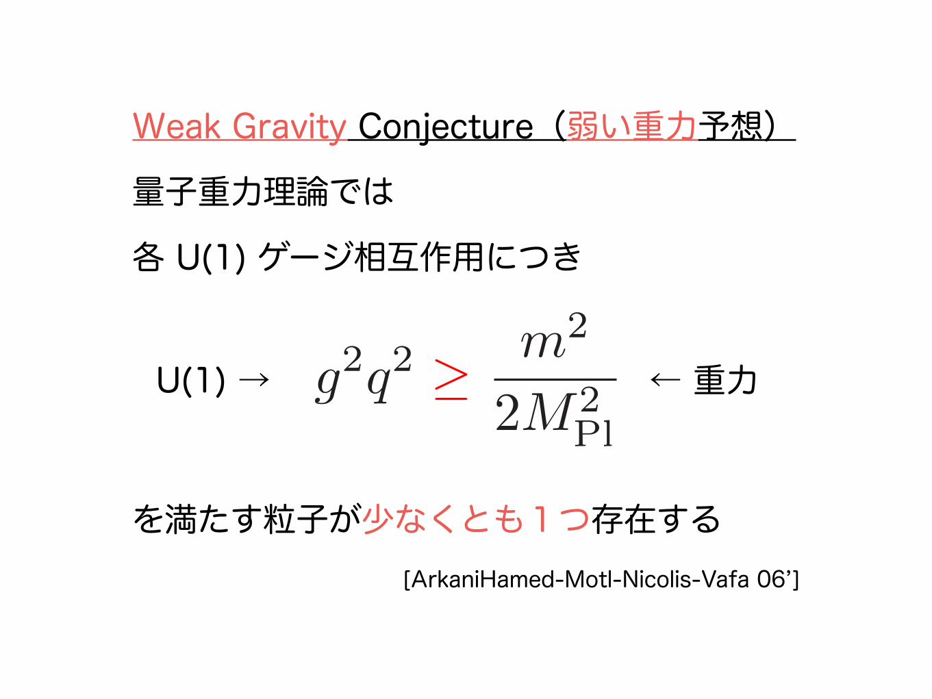
no global symmetry in 量子重力
BH蒸発
BH
の 粒子を大量注入B � L > 0 Hawking 輻射は
B � L = 0
BH の蒸発を考えると、global symmetry charge は保存しない
→ global symmetry は存在したとしても近似的対称性!
cf. ゲージ対称性の場合は電場の影響で Hawking 輻射は中性でない

このように、弦理論(より一般に量子重力)を考えると
理論の持つ対称性や matter contents に非自明な制限
→ Landscape と Swampland [Vafa ’06]

QFT CQFT A QFT B
swampland: 重力を考えなければ無矛盾な理論だが、 量子重力とは無矛盾に couple できない
landscape: 量子重力と整合的な場の量子論的模型

landscapeswampland
boundaries!
- Landscape と Swampland の境界を決める条件な何か??
- その現象論的帰結は??(量子重力への現象論的手がかり!)
Swampland program

plan
1. Introduction: Landscape と Swampland
2. Weak Gravity Conjecture とその拡張
3. Inflation 模型への示唆
4. まとめと展望
✔

2. Weak Gravity Conjecture とその拡張

Weak Gravity Conjecture[ArkaniHamed-Motl-Nicolis-Vafa 06’]

global symmetry = gauge symmetry @ g = 0
→ gauge coupling g への定量的下限はあるか??
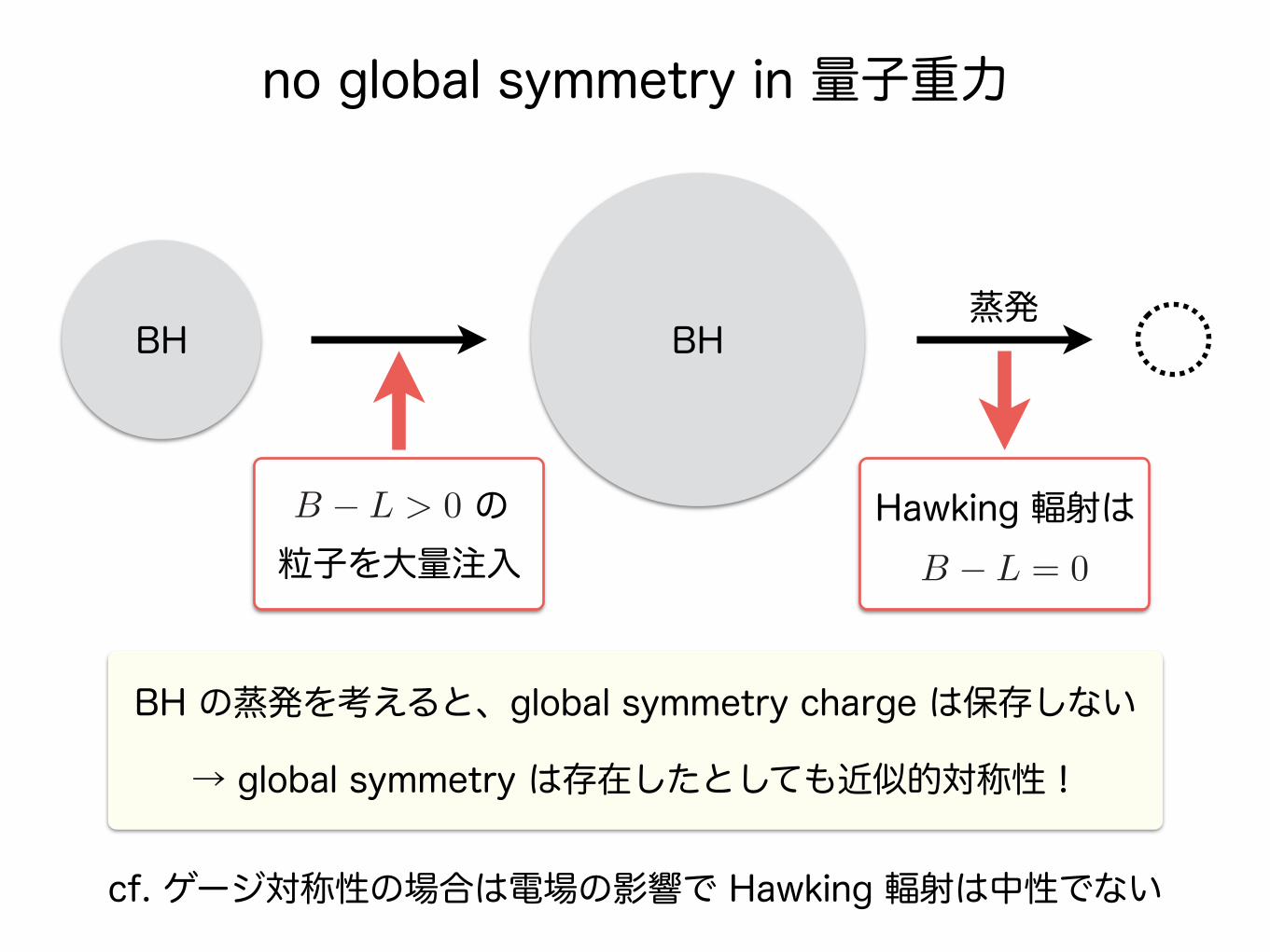
2) extremal BH:
T = 0; Hawking 輻射を出さない → 別の崩壊機構を持たない限りは安定に存在し続ける
g|Q| = M/p2MPl
※ は裸の特異点 (cf. cosmic censorship)g|Q| > M/p2MPl
Einstein-Maxwell 理論におけるブラックホール
1) sub-extremal BH:
T ≠ 0 の Hawking 輻射を出して extremal BH に崩壊
g|Q| < M/p2MPl

[ArkaniHamed-Motl-Nicolis-Vafa 06’] が提案した作業仮説:
対称性(ex. SUSY)で守られていない extremal BH は 何かしらの崩壊チャンネルを持つべし!
- 対称性で守られていない安定状態が無数にあるのは不思議
- entropy bound (conjecture) との相性が悪い
Q
M
裸の特異点裸の特異点
no Hawking radiationno Hawking radiation
Hawking 輻射で崩壊

Weak Gravity Conjecture
a particle q � m
extremal BHQ = M
BH’Q� q M �m
[ArkaniHamed-Motl-Nicolis-Vafa 06’]
簡単のため な単位系Qext
= Mext
extremal BH が崩壊チャンネルを持ち、
かつ崩壊した後のBHが裸の特異点を持たない
→ を満たす粒子が少なくとも1つ存在q � m

Weak Gravity Conjecture
a particle q � m
extremal BHQ = M
BH’Q� q M �m
[ArkaniHamed-Motl-Nicolis-Vafa 06’]
簡単のため な単位系Qext
= Mext
extremal BH が崩壊チャンネルを持ち、
かつ崩壊した後のBHが裸の特異点を持たない
→ を満たす粒子が少なくとも1つ存在gq � mp2MPl

- 弦理論の具体例で様々なチェック
- AdS/CFT を用いた理解
- 今のところ反例は知られていない
[Nakayama-Nomura ’15, Harlow ’15, Benjamin et al ’16, Montero et al ’16, …]
[Brown et al ’15, Heidenreich et al ’15, Hebecker-Soler ’17, Montero et al ’17, …]

Q. extremal BH が崩壊すべしという作業仮説はどうやねん??

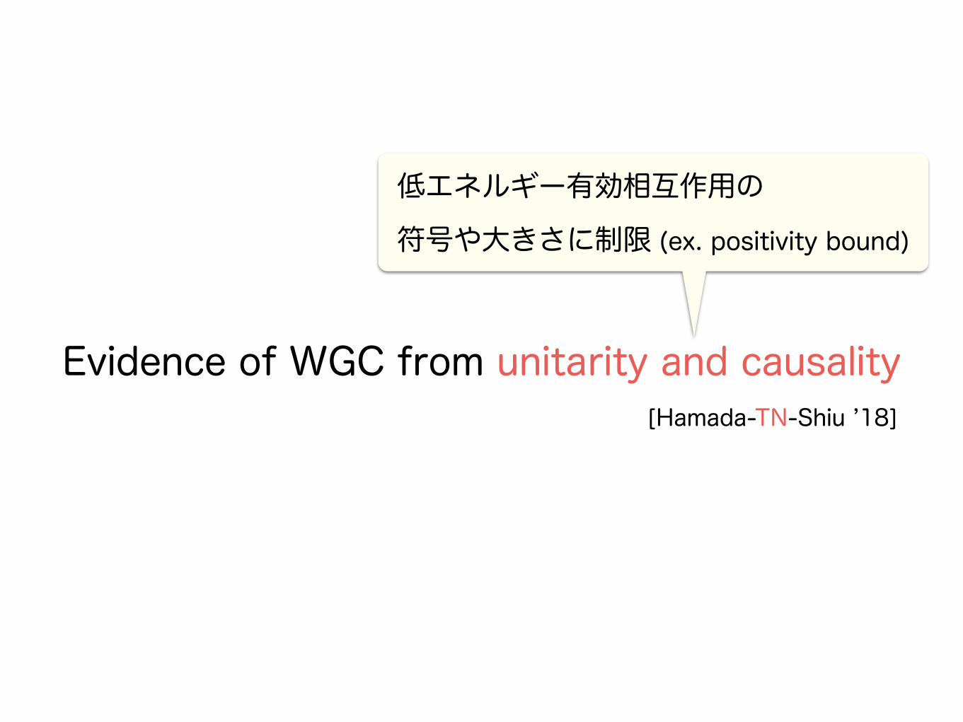
Evidence of WGC from unitarity and causality[Hamada-TN-Shiu ’18]
Evidence of WGC from unitarity and causality[Hamada-TN-Shiu ’18]
低エネルギー有効相互作用の 符号や大きさに制限 (ex. positivity bound)

高階微分項の符号によっては を満たす BH が存在!g|Q| > Mp2MPl
[Kats-Motl-Padi ’06]

Q
M
裸の特異点裸の特異点
no Hawking radiationno Hawking radiation
Hawking 輻射で崩壊
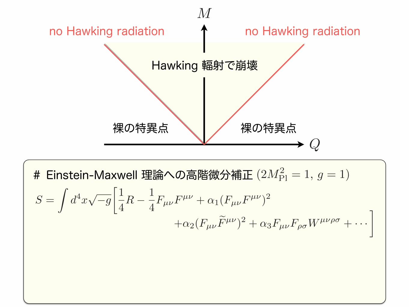
# Einstein-Maxwell 理論への高階微分補正 (2M2Pl = 1, g = 1)
+↵2(Fµ⌫eFµ⌫)2 + ↵3Fµ⌫F⇢�W
µ⌫⇢� + · · ·�S =
Zd
4x
p�g
1
4R� 1
4Fµ⌫F
µ⌫ + ↵1(Fµ⌫Fµ⌫)2
Q
M
裸の特異点裸の特異点
no Hawking radiationno Hawking radiation
Hawking 輻射で崩壊

# Einstein-Maxwell 理論への高階微分補正 (2M2Pl = 1, g = 1)
+↵2(Fµ⌫eFµ⌫)2 + ↵3Fµ⌫F⇢�W
µ⌫⇢� + · · ·�S =
Zd
4x
p�g
1
4R� 1
4Fµ⌫F
µ⌫ + ↵1(Fµ⌫Fµ⌫)2
→ BH 解や事象の地平線の構造が修正される:
|Q|M
1 +2
5
(4⇡)2
Q2(2↵1 � ↵3) +O(1/Q4) なら裸の特異点なし!
Q
M
裸の特異点裸の特異点
no Hawking radiationno Hawking radiation
Hawking 輻射で崩壊

Q
M
裸の特異点裸の特異点
no Hawking radiationno Hawking radiation
Hawking 輻射で崩壊
# Einstein-Maxwell 理論への高階微分補正 (2M2Pl = 1, g = 1)
+↵2(Fµ⌫eFµ⌫)2 + ↵3Fµ⌫F⇢�W
µ⌫⇢� + · · ·�S =
Zd
4x
p�g
1
4R� 1
4Fµ⌫F
µ⌫ + ↵1(Fµ⌫Fµ⌫)2
→ BH 解や事象の地平線の構造が修正される:
|Q|M
1 +2
5
(4⇡)2
Q2(2↵1 � ↵3) +O(1/Q4) なら裸の特異点なし!
2↵1 � ↵3 > 0 なら|Q| > M の BH!

を示せれば WGC の存在証明!2↵1 � ↵3 > 0

+↵2(Fµ⌫eFµ⌫)2 + ↵3Fµ⌫F⇢�W
µ⌫⇢� + · · ·�S =
Zd
4x
p�g
1
4R� 1
4Fµ⌫F
µ⌫ + ↵1(Fµ⌫Fµ⌫)2
Evidence of WGC from unitarity and causality[Hamada-TN-Shiu ’18]
① は対称性や causality でかなり縛られる↵3
SUSY: ↵3 = 0, non-SUSY: |↵1|, |↵2| � |↵3|
�+
�+
h+2↵3
causality constraint [cf. Camanho-Edelstein-Maldacena-Zhiboedov ’14]
② の符号は unitarity で縛られる↵1
ex. dilaton coupling�
fFµ⌫F
µ⌫ → dilaton を積分 → 有効相互作用1
2m2f2(Fµ⌫F
µ⌫)2

仮に を満たす粒子がいなくても
dilaton や moduli などの効果で
→ を満たす BH が存在
|q| � m
2↵1 � ↵3 ' 2↵1 > 0
|Q| � M
※ WGC および “extremal BH は崩壊すべし” の強い証拠
causalityunitarity

Weak Gravity Conjecture の拡張

# Tower/(sub)Lattice Weak Gravity Conjecture[Heidenreich et al ’15 & ’16, Montero et al ’16, Andriolo-Junghans-TN-Shiu ’18]
q1
q2
を満たす粒子がタワー/格子状に無限個存在|~q| � m
- BH argument + KK reduction [Heidenreich et al ’15]
- positivity + KK reduction [Andriolo-Junghans-TN-Shiu ’18]- modular invariance [Heidenreich et al ’16, Montero et al ’16]
# p-form ゲージ場への一般化
p-form ゲージ場:
結合している (p-1)-dim object の張力に上限 T . (g2MD�2Pl )1/2
※ axion を 0-form ゲージ場とみなすと
instanton action と axion decay constant に Sinst ·f
MPl. 1

plan
1. Introduction: Landscape と Swampland
2. Weak Gravity Conjecture とその拡張
3. Inflation 模型への示唆
4. まとめと展望
✔
✔

3. Inflation 模型への示唆

reality, inflation ends at some finite time, and the approximation (60) although valid at early times,breaks down near the end of inflation. So the surface ⇥ = 0 is not the Big Bang, but the end ofinflation. The initial singularity has been pushed back arbitrarily far in conformal time ⇥ ⇤ 0, andlight cones can extend through the apparent Big Bang so that apparently disconnected points arein causal contact. In other words, because of inflation, ‘there was more (conformal) time beforerecombination than we thought’. This is summarized in the conformal diagram in Figure 9.
6 The Physics of Inflation
Inflation is a very unfamiliar physical phenomenon: within a fraction a second the universe grewexponential at an accelerating rate. In Einstein gravity this requires a negative pressure source orequivalently a nearly constant energy density. In this section we describe the physical conditionsunder which this can arise.
6.1 Scalar Field Dynamics
reheating
Figure 10: Example of an inflaton potential. Acceleration occurs when the potential energy ofthe field, V (⇤), dominates over its kinetic energy, 1
2 ⇤̇2. Inflation ends at ⇤end when thekinetic energy has grown to become comparable to the potential energy, 1
2 ⇤̇2 ⇥ V . CMBfluctuations are created by quantum fluctuations �⇤ about 60 e-folds before the end ofinflation. At reheating, the energy density of the inflaton is converted into radiation.
The simplest models of inflation involve a single scalar field ⇤, the inflaton. Here, we don’tspecify the physical nature of the field ⇤, but simply use it as an order parameter (or clock) toparameterize the time-evolution of the inflationary energy density. The dynamics of a scalar field(minimally) coupled to gravity is governed by the action
S =⇤
d4x⌅�g
�12R +
12gµ⇥⇧µ⇤ ⇧⇥⇤� V (⇤)
⇥= SEH + S⇤ . (61)
The action (61) is the sum of the gravitational Einstein-Hilbert action, SEH, and the action of ascalar field with canonical kinetic term, S⇤. The potential V (⇤) describes the self-interactions of the
31
Inflation in a nutshell
- 平坦なポテンシャルを持つスカラー場 “inflaton” を導入
- inflation 中の量子揺らぎ = CMB 温度揺らぎなどの構造の起源
※ CMB の観測などからインフラトンポテンシャル V がわかる

Planck Collaboration: Constraints on inflation 55
Fig. 54. Marginalized joint 68 % and 95 % CL regions for ns and r0.002 from Planck alone and in combination with its cross-correlation with BICEP2/Keck Array and/or BAO data compared with the theoretical predictions of selected inflationary models.
further improving on the upper limits obtained from the differentdata combinations presented in Sect. 5.
By directly constraining the tensor mode, the BKP likeli-hood removes degeneracies between the tensor-to-scalar ratioand other parameters. Adding tensors and running, we obtain
r0.002 < 0.10 (95 % CL, Planck TT+lowP+BKP) , (168)
which constitutes almost a 50 % improvement over the PlanckTT+lowP constraint quoted in Eq. (28). These limits on tensormodes are more robust than the limits using the shape of theCTT` spectrum alone owing to the fact that scalar perturbations
cannot generate B modes irrespective of the shape of the scalarspectrum.
13.1. Implications of BKP on selected inflationary models
Using the BKP likelihood further strengthens the constraintson the inflationary parameters and models discussed in Sect. 6,as seen in Fig. 54. If we set ✏3 = 0, the first slow-roll pa-rameter is constrained to ✏1 < 0.0055 at 95 % CL by PlanckTT+lowP+BKP. With the same data combination, concave po-tentials are preferred over convex potentials with log B = 3.8,which improves on log B = 2 obtained from the Planck dataalone.
Combining with the BKP likelihood strengthens the con-straints on the selected inflationary models studied in Sect. 6.Using the same methodology as in Sect. 6 and adding the BKPlikelihood gives a Bayes factor preferring R2 over chaotic in-flation with monomial quadratic potential and natural inflationby odds of 403:1 and 270:1, respectively, under the assumptionof a dust equation of state during the entropy generation stage.The combination with the BKP likelihood further penalizes thedouble-well model compared to R2 inflation. However, adding
Table 17. Results of inflationary model comparison using thecross-correlation between BICEP2/Keck Array and Planck. Thistable is the analogue to Table 6, which did not use the BKP like-lihood.
Inflationary Model ln B0X
wint = 0 wint , 0
R + R2/6M2 . . . +0.3n = 2 �6.0 �5.6Natural �5.6 �5.0Hilltop (p = 2) �0.7 �0.4Hilltop (p = 4) �0.6 �0.9Double well �4.3 �4.2Brane inflation (p = 2) +0.2 0.0Brane inflation (p = 4) +0.1 �0.1Exponential inflation �0.1 0.0SB SUSY �1.8 �1.5Supersymmetric ↵-model �1.1 +0.1Superconformal (m = 1) �1.9 �1.4
BKP reduces the Bayes factor of the hilltop models comparedto R2, because these models can predict a value of the tensor-to-scalar ratio that better fits the statistically insignificant peak atr ⇡ 0.05. See Table 17 for the Bayes factors of other inflationarymodels with the same two cases of post-inflationary evolutionstudied in Sect. 6.
13.2. Implications of BKP on scalar power spectrum
The presence of tensors would, at least to some degree, requirean enhanced suppression of the scalar power spectrum on largescales to account for the low-` deficit in the CTT
` spectrum. Wetherefore repeat the analysis of an exponential cut-off studied
deviation from scale invariance
primordial gravitatio
nal w
aves
インフラトンポテンシャルへの観測的制限
natural inflation は large field inflation の simple な模型
this one!

natural inflation: axion = inflaton
# natural inflation [Freese-Frieman-Olinto ’90]
アクシオンの典型的 Lagrangian:
L = �1
2(@µ�)
2 � V (�)
V (�) / e�Sinst
✓1� cos
�
f
◆+
X
n�2
e�nSinst
✓1� cos
n�
f
◆
Sinst
f- : アクシオン崩壊係数 ~ (結合定数)
- アクシオンポテンシャルは周期的
- : instanton 作用 ~ tension
-1
� ! �+ 2⇡f

2⇡f
slow-roll axion potential
インフレーション期を一定時間保つ
→ インフラトンポテンシャルが十分平坦 (slow-roll condition)
f > MPl
- negligible higher harmonics ( ) →
- long enough periodicity →
n � 2 Sinst > 1
V (�) / e�Sinst
✓1� cos
�
f
◆+
X
n�2
e�nSinst
✓1� cos
n�
f
◆
�
V (�)

WGC は を要求
→ simple な axion inflation 模型は禁止される
Sinst ·f
MPl. 1

loophole と予言

- large field inflation を
および で実現Vs.r. e�S0inst
✓1� cos
�
f 0
◆(f 0 > MPl)
- WGC は な instanton で満たされる
→ ポテンシャルの振動 → power spectrum の振動&non-Gaussianity
Sinst ·f
MPl. 1
axion monodromy
ポテンシャルを多価関数にする
V (�) = Vs.r.(�) + e�Sinst
✓1� cos
�
f
◆
spectator instanton
WGC を満たすためだけに instanton を導入
V (�) = e�Sinst
✓1� cos
�
f
◆+ e�S0
inst
✓1� cos
�
f 0
◆

Tower/(sub)Lattice WGC からの implication

# 異なる崩壊係数を持つ isntanton が多数存在すべし!
( i:instanton のラベル)V (�) =X
i
e�Sicos
✓�
fi+ �i
◆

5
-6 -4 -2 2 4 6
0.5
1.0
1.5
2.0
2.5
3.0
0
0.9
0.8
0.7
(natural inflation)
q=0
FIG. 4. The inflaton potential V (φ) with the Jacobi thetafunction given by Eq. (22) for q = 0, 0.7, 0.8 and 0.9 frombottom to top.
0.92 0.94 0.96 0.98 1.00
10-4
0.001
0.01
0.1
0.90
r
ns
q=0
0.4
0.6
0.7 0.8
R inflation2
FIG. 5. (ns, r) for the theta inflation with the potential (22).
C. Inflation with Dedekind eta function
Now we study an inflation model with the Dedekindeta function,
η(τ) = q1
12
∞!
n=1
(1− q2n), (24)
where q = eiπτ and Im(τ) > 0. It is known that theeta function is given by the special values of the thetafunctions, for instance, η3(τ) = 1
2ϑ2(0, τ)ϑ3(0, τ)ϑ0(0, τ).To be specific, we will study the inflaton potential:
V (φ) = −Λ4
"
η−2
#
6
πFφ+ iC
$
+ c.c.
%
+ const.,(25)
∝ cosφ
F+ e−2πC cos
#
11φ
F
$
+ · · · ,
where C is a real parameter, and the constant term isadded so as to make the inflaton potential vanish at theorigin, V (0) = 0. In the second line, we have expandedthe eta function in terms of |q| = e−πC ≪ 1. The inflaton
1 2 5 10 20 500.90
0.92
0.94
0.96
0.98
1.00
ns
F / Mp
q=0 (natural inflation)0.40.6
0.7
0.8
1 2 5 10 20 50
1 10- 4
5 10- 4
0.001
0.005
0.01
0.05
0.1
x
x
r
F / Mp
q=0
0.4
0.6
0.70.8
FIG. 6. Same as Fig. 3 but for the theta inflation (22).
potential (25) is shown in Fig. 7 for several values of C.One can see from the figure that the inflaton potentialhas a maximum at φ = πF and it receives modulationsfor C ! 1. Here, (φ, C) = (0, 1) implies the self-dualpoint under the modular transformation of τ → −1/τ ,i.e., C → 1/C. For larger values of C, the above poten-tial asymptotes to the natural inflation with the decayconstant F , as one can see from the expansion of theinflaton potential. Note that the normalization of thepotential height is chosen for visualization purpose. Thisdoes not affect the predicted values of r, ns and its run-ning in the following analysis.
The predicted values of ns and r are shown in Fig. 8for C = 1.5, 1 and 0.85, where we have varied the valueof the decay constant F , and set the e-folding numberN to be 60. For C = 1 and C = 0.85, the predictedvalues of (ns, r) rotate counterclockwise as F decreases.In contrast to the previous two cases, this model does notasymptote to the exponential inflation. The dependenceof ns and r on the decay constant F is shown in Fig. 9,and we find that the super-Planckian decay constant isrequired to be consistent with the Planck data. We willreturn to the issue of super-Planckian decay constant atthe end of this section.
Finally let us evaluate the running of the spectral in-dex, dns/d ln k. Recently the inflation model with theDedekind eta function was shown to generate a sizablerunning of the spectral index [41]. The running can be
# 異なる崩壊係数を持つ isntanton が多数存在すべし!
( i:instanton のラベル)V (�) =X
i
e�Sicos
✓�
fi+ �i
◆
# Elliptic Inflation [Higaki-Takahashi ’15]
natural inflation と plateau inflation (small field) を interpolate

5
-6 -4 -2 2 4 6
0.5
1.0
1.5
2.0
2.5
3.0
0
0.9
0.8
0.7
(natural inflation)
q=0
FIG. 4. The inflaton potential V (φ) with the Jacobi thetafunction given by Eq. (22) for q = 0, 0.7, 0.8 and 0.9 frombottom to top.
0.92 0.94 0.96 0.98 1.00
10-4
0.001
0.01
0.1
0.90
r
ns
q=0
0.4
0.6
0.7 0.8
R inflation2
FIG. 5. (ns, r) for the theta inflation with the potential (22).
C. Inflation with Dedekind eta function
Now we study an inflation model with the Dedekindeta function,
η(τ) = q1
12
∞!
n=1
(1− q2n), (24)
where q = eiπτ and Im(τ) > 0. It is known that theeta function is given by the special values of the thetafunctions, for instance, η3(τ) = 1
2ϑ2(0, τ)ϑ3(0, τ)ϑ0(0, τ).To be specific, we will study the inflaton potential:
V (φ) = −Λ4
"
η−2
#
6
πFφ+ iC
$
+ c.c.
%
+ const.,(25)
∝ cosφ
F+ e−2πC cos
#
11φ
F
$
+ · · · ,
where C is a real parameter, and the constant term isadded so as to make the inflaton potential vanish at theorigin, V (0) = 0. In the second line, we have expandedthe eta function in terms of |q| = e−πC ≪ 1. The inflaton
1 2 5 10 20 500.90
0.92
0.94
0.96
0.98
1.00
ns
F / Mp
q=0 (natural inflation)0.40.6
0.7
0.8
1 2 5 10 20 50
1 10- 4
5 10- 4
0.001
0.005
0.01
0.05
0.1
x
x
r
F / Mp
q=0
0.4
0.6
0.70.8
FIG. 6. Same as Fig. 3 but for the theta inflation (22).
potential (25) is shown in Fig. 7 for several values of C.One can see from the figure that the inflaton potentialhas a maximum at φ = πF and it receives modulationsfor C ! 1. Here, (φ, C) = (0, 1) implies the self-dualpoint under the modular transformation of τ → −1/τ ,i.e., C → 1/C. For larger values of C, the above poten-tial asymptotes to the natural inflation with the decayconstant F , as one can see from the expansion of theinflaton potential. Note that the normalization of thepotential height is chosen for visualization purpose. Thisdoes not affect the predicted values of r, ns and its run-ning in the following analysis.
The predicted values of ns and r are shown in Fig. 8for C = 1.5, 1 and 0.85, where we have varied the valueof the decay constant F , and set the e-folding numberN to be 60. For C = 1 and C = 0.85, the predictedvalues of (ns, r) rotate counterclockwise as F decreases.In contrast to the previous two cases, this model does notasymptote to the exponential inflation. The dependenceof ns and r on the decay constant F is shown in Fig. 9,and we find that the super-Planckian decay constant isrequired to be consistent with the Planck data. We willreturn to the issue of super-Planckian decay constant atthe end of this section.
Finally let us evaluate the running of the spectral in-dex, dns/d ln k. Recently the inflation model with theDedekind eta function was shown to generate a sizablerunning of the spectral index [41]. The running can be
# 異なる崩壊係数を持つ isntanton が多数存在すべし!
( i:instanton のラベル)V (�) =X
i
e�Sicos
✓�
fi+ �i
◆
# Elliptic Inflation [Higaki-Takahashi ’15]
natural inflation と plateau inflation (small field) を interpolate
# Tower/sub(Lattice) WGC に motivate されて
stringy setup を色々調べるのもありかも(既にやりつくしました?> 檜垣さん)

4. まとめと展望

Web of Weak Gravity Conjectures
no global symmetry
Tower/(sub)Lattice Weak Gravity Conjecture
不等式を満たす粒子がタワー/格子状に無限個存在[Heidenreich et al ’16, Montero et al ’16, Andriolo-Junghans-TN-Shiu ’18]
Weak Gravity Conjecture [ArkaniHamed-Motl-Nicolis-Vafa 06’]
9 a particle satisfying gq � m/p2MPl
※ axion への拡張は inflation の模型構築に効いてくる

今日扱わなかった話題・展望
# WGC と dark matter
平坦過ぎるポテンシャルや小さ過ぎるゲージ相互作用は危険
→ ultra light axion DM (fuzzy DM), milicharged DM, …
# no non-SUSY AdS!? [Ooguri-Vafa ’16]
SUSY で守られてない AdS は不安定じゃないかという conjecture
→ 素粒子標準模型と beyond (ex. Majorana neutrino mass はダメ??) cf. extremal BH の near horizon limit = AdS なのでその不安定性とも関係
# de Sitter space in quantum gravity/string theory

ありがとうございました!