Embed Size (px)
Citation preview

i
Explaining What Leads Up to Stock Market Crashes: A Phase Transition Model and Scalability Dynamics
Rossitsa Yalamova
University of Lethbridge, etc.
&
Bill McKelvey
UCLAAnderson School of Management, 110 Westwood Plaza, Los Angeles, CA 90095‐1481
Phone 310‐825‐7796; Fax 310‐206‐2002; [email protected]
© Copyright. All rights reserved. Not to be quoted, paraphrased, copied, or distributed in any fashion without permission.
November 27, 2008

ii
Explaining What Leads Up to Stock Market Crashes: A Phase Transition Model and Scalability Dynamics
ABSTRACT Markets are described as complex dynamical systems that may switch between two regimes. Efficient market prevails when rational traders make decisions independently based on all available public and private information. When information complexity increases traders resort to rule based trading and imitation rate increases. As a result of this herding behavior price bubbles build up. If not reverted such behavior leads to loss of traders’ heterogeneity and at a critical point, crash occurs. Predictability of such critical points is descriobed previously as log‐periodic oscillation of prices. Multifractal analysis should detect the volatility cascade leading to crashes.

1
I. INTRODUCTION
Although Gene Fama championed the publication of Benoit Mandelbrot’s article in the Journal of
Business in 1963, he also wrote a critique and thence stayed on the path of the three dominant Finance
paradigms, the efficient market hypothesis (EMH; Fama, 1970), the capital‐asset pricing model (CAPM;
Sharpe, 1964; Lintner, 1965; & Black, 1972), and the Black‐Scholes (1973) options‐pricing model. In
parallel, Mandelbrot (1970, 1982, 1997, 1999, Mandelbrot & Hudson, 2004) kept applying his fractal
geometry ideas to stock markets. His views have more recently been picked up by others (Peters, 1991,
1994; Rosser, 2000; Sornette, 2003; Malevergne & Sornette, 2005; Jondeau et al., 2007; Calvert and
Fisher, 2008). Over the years these two competing Schools have remained contentious, seemingly
arguing about the same turf, with little basis of reconciliation apparent. For example, in his 2004 book
with Hudson, Mandelbrot says: “‘Modern’ financial theory is founded on a few, shaky myths that lead us
to underestimate the real risk of financial markets” and: “Orthodox financial theory is riddled with false
assumptions and wrong results” (pp. ix, x). According to Fama (1998), however, until new and better
paradigm is put forth, one cannot criticize EMH/CAPM. Fama reduces behavioral finance–and trading
dynamics—to anomalies and over‐/under reaction episodes that are normally distributed.
The mathematical descriptions of financial market behavior by each School are now equally robust.
Still, EMH and other paradigms have successfully remained at the center of market analysis for most
researchers in the Finance community, even though the Fractal School has continued to grow in
numbers of participants and depth of mathematical analysis (Adler, Feldman & Taqqu, 1998; Rachev &
Mittnik, 2000; Malevergne & Sornette, 2005; Jondeau, Poon, & Rockinger, 2006). Since we have just
passed through another of what Martin Greenspan recently termed a once-in-a-century market crash (the
first being the 1929 crash) our concern about what sets off unusual volatility sequences and occasional
extreme crashes is surely timely and calls for further analysis of when and why the EMH view of market
trading shifts into behaviors better fitting fractal mathematics.

2
Following EMH, we first distinguish between the rational and noise traders who, acting independently
of each other, create efficient markets. Then we recognize interdependent trader behaviors, recently
accounted for in the mathematics of what Malevergne and Sornette (2005, p. 100) call the “copula” of
two random variables—which offers a “complete and unique description of the dependence structure
existing between them.” First, we note that there are three kinds of equally relevant trading behaviors
that our models and theories have to account for: (a) There are two kinds of trader behavior in which
they act independently of each other, which are excellently represented by the formalizations of EMH—
which includes both rational and noise traders; and (b) A third kind of trader behavior also exists—
where trader behaviors are in fact interdependent. We will call this the high‐risk trading category; it
occurs when traders resort to rule‐driven behavior—e.g., chartists, herding, information cascades, etc.—
in short: behavioral traders. Second, we note, however, that Sornette and his colleagues are content to
draw explanatory closure when they fit an equation to a few parameters representing log periodic
oscillations of prices (Sornette, 2004). A number of quantitative researchers now fit extreme events into
power law distributions of price changes to formalize non‐linear patterns during periods of extreme
volatility (e.g., Jondeau et al., 2007; Calvet and Fisher, 2008). But our question remains: What are the
various kinds of interdependent trader‐induced causes that scale up into the fractal volatility sequences
and occasional extreme events (crashes) we see in stock market behaviors?
We do not offer an alternative to EMH/CAPM but extend the existing efficient market framework to
accommodate situations with higher information complexity, interactions with positive feedback, and
extreme events that cannot be simply explained by presuming independent‐additive data points, and
normal distributions. For example, the development of the “herding behavior” literature in finance
(Banerjee, 1992; Bikhchandani, et al. 1992; Prechter, 1999; Brunnermeier, 2001; Rook, 2006;) marks a
significant recognition that interdependent trader behavior may result in skew distributions of stock
market prices and, therefore, offers the first underlying explanation of behavior that may begin as

3
Holland’s (2002) “tiny initiating events,” but later scales up into extremes. Building on this, we introduce
several so‐called “scale‐free theories” that explain why some tiny events scale up into extremes while
many others do not. In all of these, interdependent trader behavior is the critical element. Our scale‐
free theories come from a range of disciplines (Andriani & McKelvey, forthcoming).
We can explain why some herding lunges scale up and then die off whereas others scale up into
significant crashes. Given the empirical base of each theory, we believe we can offer rather solid
rationale as to why high‐risk trading behavior is ever present as mild to fairly strong volatility cycles.
Thus, interactions of many traders with different investment horizons may simply die out, while some
others may scale up into significant crashes that may or may not result from macroeconomic events
(Rosser, 2000). Which way it goes depends on the nature of exogenous and endogenous shocks
(Sornette and Helmstetter, 2003). Any shock that is related to small events with cumulative effects
(endogenous) has different price diffusion than an exogenous shock such as 9/11, a natural disaster, a
political coup, or some shocking economic news such as the 2007 liquidity crisis. Standard economic
theory postulates that continuous streams of news get incrementally incorporated into prices. In
principle, large shocks should result from anomalous, very bad news, but the puzzle around 1987 is that
there was no such news. Large market moves and strong bursts of volatility are not, then, always
associated with external economic, political or natural events (White, 1996). Endogenous shocks can
result from the combination and/or accumulation of many small shocks as what seems like random
noise re‐structures into different kinds of nonlinearities (Schroeder, 1991).
In this paper, we attempt to further legitimate the separate‐but‐equal status of EMH and Fractal
Finance (FF). We do this by attempting to go beyond classic financial asset pricing theory to account for
findings of behavioral aberrations arising where unrealistic assumptions are made of unbounded
rationality and independent judgments among investors about future payoffs and choices made solely
on those anticipated payoffs (Fama & French, 2007).

4
The objective of this paper is to encourage research on the nonlinear models giving some theoretical
underpinning to the equations that mirror markets as complex dynamical systems. Instead of just an
“either‐or” view of EMH or FF, we especially focus on dynamics causing traders to shift from one regime
to the other. Research of extreme events, and underlying scale‐free dynamics, is of particular interest
for the overall understanding of markets functioning as complex systems reveal their characteristics
under stress better than in normal conditions. Baum and McKelvey (2006) also reveal the potential
advantage of extreme value theory in modeling management phenomena and the increasing popularity
in financial applications. Andriani and McKelvey (2007) reveal how misleading are the assumptions
behind the econometric methods involving linear multiple regression.
We begin by reviewing both the EMH and FF views of market dynamics. Then we use a physical
analogy to help define the axes of our “Financial Markets Phase Diagram.” In this diagram we depict and
define the Triple Point where we see EMH‐driven behaviors and the Critical Point at which major market
crashes occur: i.e., 1929, 1987, and 2007+. We then turn our attention toward explaining the various
kinds of nonlinearities in trader behavior occurring as “market mania” develops. We define four kinds of
nonlinearities. We then apply concepts from complexity science, econophysics, and scale‐free theory to
zero in on the underlying causes of these market nonlinearities. A Conclusion follows.
II. BACKGROUND
EFFICIENT MARKET HYPOTHESIS
According to the efficient markets hypothesis (EMH) that dominates finance theory and empirical
work, price changes are completely random and driven by unexpected news about fundamentals, i.e.
EMH models belong to the class of theories of asset price dynamics which consider fluctuations to be a
result of exogenous stochastic influences. Efficient markets imply the absence of detectable (and
predictable) structure in the market. If markets are not efficient, then we should be able to find

5
structure in financial data and exploit it. While some evidence against efficiency can be found, empirical
studies generally don't find structure that is exploitable.
A basic principle in modeling the stock market is rationality. Traders in general exhibit a rational
behavior, trying to optimize their strategies based on the available information. However this behavior is
only "boundedly rational" since the available information is incomplete and traders have limited abilities
to process the available information. The process of decision‐making is essentially "noisy". In fact, a
noise free market with rational traders of infinite analyzing abilities would have very little trading, if any,
since for a market to be active there should be individuals willing to take opposite sides of the trade for
the same price based on differing assumptions about where the price is going next. Perfect information
and analytical ability would inevitably lead all traders to the same assumptions.
Fama and French (2007) assert how disagreement and tastes can affect asset prices thus admitting
that some assumptions in standard asset pricing models are unrealistic. Recent models emphasize the
role of heterogeneous beliefs and expectations about future prices. Brock and Holmes (1998) recap two
basic investor types in these heterogeneous agent models: 1) rational traders including buy and hold
fundamentalists (who base their trades on the perceived intrinsic value of firms) and 2) noise traders
who are basically chartists or technical market analysts, and others who trade on misperceived
information, rumors, personal opinions, or who simply copy other traders with positive reputations. We
may also include liquidity traders here, i.e. traders whose decision to “cash out” is based on a need for
liquidity that is independent of market information.
Equilibrium theory is based on four assumptions a) price taking, where agents can not do anything to
change the price; b) independent agents make utility maximizing decisions; c) market clearing, e.g.
equality of aggregate demand and supply and d)rational decisions based on perfect information.

6
When efficient market rules, it sustains dynamic equilibrium and temporary deviations are viewed as
anomalies that are randomly distributed, therefore predictions are impossible and nobody can
consistently beat the market.
FRACTAL FINANCE—CHAOS
Complexity has always been part of our environment and many scientific fields have dealt with
complex systems, which display variation without being purely random. Complex systems tend to be
high dimensional and non‐linear but may exhibit low‐dimensional behavior. Financial markets have been
shown to be similar to complex dynamical systems (Johansen et al., 2000). The different parts of
complex systems are linked and thus affect one another. A complex system may exhibit deterministic
and random characteristics with the level of complexity depending on the system's dynamics and its
interactions with the environment.
One of the objectives in quantifying complex systems is to explain emergent structures, i.e. self‐
organization. Phase transition is a property of self‐organizing systems that move from static or chaotic
states to a semi‐stable balance between these two states that can be more effective (Brown and
Eisenhardt, 1998). Self‐organized criticality is characterized by power‐law distribution of events around
the phase boundary. Sornette et al. (1996) argue that scale invariance and self‐similarity are dominant
concepts useful in describing the processes surrounding the October 1987 crash since this event could
be seen as the result of a worldwide cooperative phenomenon, analogous to a critical phase transition
in physics. Johansen et al. (2000) identify patterns of near‐critical behavior years before market crashes.
Similarly, the hierarchical or cascade model of traders with "crowd" or "herd" behavior illustrates the
concept of criticality (Bak, 1996), where a large proportion of the actors simultaneously decide to sell
their stocks (cf. Breymann et al., 2000).
Another piece of the puzzle is the observation of aperiodic long‐term behavior that exhibits sensitive
dependence on initial conditions and has limited predictability of the dynamics—characteristics of

7
chaos. This sensitivity to initial conditions means that two points in a chaotic system may move in vastly
different trajectories in their phase space, even if the difference in their initial configurations is very
small. Since some nonlinear dynamical systems under certain conditions exhibit chaos, detection of the
emergence of chaos in the system (as opposed to prediction) might allow active control at a low cost
leading not only to highly positive outcomes but also to the prevention of costly crisis situations.
In finance, Brock and Hommes (1998), Chen et al. (2001), Gaunersdorfer (2000), Lux (1995, 1998) and
others suggest that heterogeneous beliefs of market players lead to market instability and complex
endogenous price dynamics such as chaotic fluctuations. When a complex dynamical chaotic system
becomes unstable, the system may split (bifurcation) in the presence of an attractor. Chaotic attractors
are fractal and fractals have complex geometry with similarity at various scales. Such attractors may be
seen as a subset of the domain wherein attraction defines a set of initial conditions.
At the time of its discovery, the phenomenon of chaotic motion was considered a mathematical
oddity, but physicists have proven that chaotic behavior is much more widespread. Chaos is randomness
operating through deterministic laws. But the question remains whether chaos may actually produce
ordered structures and patterns that can be used in finance to make improvements over asset pricing
models that are based on the assumption of randomness.
Theories of asset pricing dynamics that challenge the EMH orthodox view see fluctuations as arising
from underlying systematic causes that can be related to nonlinear dynamic mechanisms. Such a
dynamical system approach to asset pricing was introduced by Chiarella (1992) and the need for
empirical techniques for the full range of nonlinear dynamic possibilities was suggested.
Market crashes have been explained theoretically and measured quantitatively in a variety of ways.
Sornette et al. (1996) reveal log‐periodic oscillations of index prices before significant drawdowns and
suggest a phase transition model where market crashes appear at the Critical Point. The market crash as
phase transition in Johansen and Sornette (1999) points at the analogy between the three states of a

8
physical system (solid, liquid and gas) and stock market dynamics at a "microscopic" level, where the
individual trader has only three possible actions: selling, buying or waiting.
III. THE PHYSICAL BASIS OF PHASE TRANSITION (AND CRITICALITY?)
In the physical sciences, a phase space depicts the set of states of a macroscopic physical system that
have relatively uniform chemical composition and physical properties. For water, as an example, the
three phases (solid, liquid, and gas) are defined by temperature/pressure combinations. The different
phases of a system may be represented using a phase diagram (Figure 1). The Triple Point is the
combination of temperature and pressure that permits the co‐existence of the three phases in dynamic
equilibrium. A phase transition, (or phase change) is the transformation of a thermodynamic system
from one phase to another. At the Critical Point, a second order phase transition occurs leading to the
disappearance of the phase boundary and the presence of a super‐critical liquid / gas state.
Figure 1: Phase Diagram

9
When a system transitions from one phase to another, there will generally be a stage where the free
energy is non‐analytic. Due to this non‐analyticity, the free energies on either side of the transition are
two different functions, so one or more thermodynamic properties will behave very differently after the
transition. The property most commonly examined in this context is the heat capacity of the substance.
During a transition, heat capacity may become infinite, jump abruptly to a different value, or exhibit a
"kink" or discontinuity in its derivative, i.e. experience an abrupt sudden change in heat capacity with
only a small change in temperature (Figure 2). Similarly, we can illustrate the change of compressibility
along the changes in pressure.
Figure 2: Heat Capacity and Compressibility changes at the phase boundary
IV. FROM PHYSICS TO FINANCE: A PHASE‐TRANSITION MODEL
In an auction, market price is determined by demand and supply, i.e. buy and sell orders. The balance
between the two we define as net demand. Balanced net demand or “0” will determine a “wait” phase
in the market. Transactions would not impact price. (As we are trying to explain market crashes as
Critical Points we find that the analogy between sell/liquid and buy/gas would agree with Sornette
(2003) description of critical market crashes. We could defend our choice of phase analogy but we’ll
spare technical details here in the initial draft.) When the demand is positive, the market is in “buy”

10
phase and conversely, a negative net demand indicates a “sell” market. Autonomous agents with
heterogeneous information and bounded analytical abilities place their orders to buy and sell securities.
At a macro level, the balance of these trading orders determines the phase of the market, i.e. the
buy/sell decision ratio divides the plane. The phase diagram should be able to explain the origin of this
balance with appropriately chosen variables on the x and y axis.
DEFINING THE AXES
Returning to our two types of investors (rational and noise), rational investors evaluate all available
information and make their trading decisions based on fundamental analysis of discounted future cash
flows, defining underpriced (buy) and overpriced (sell) stocks. In the CAPM Return/Risk ratio is linear,
that allows us to represent the same notion of ranking from under to overpriced using a
risk/fundamentals ratio. Relative risk increase should suggest prevalence of “sell” decision under the
efficient market hypothesis. Thus the y‐axis of our financial markets phase diagram (Figure 3) measures
a risk/fundamentals ratio.
On the x‐axis, we replace temperature with the Noise to Information trading ratio. In the physical
phase transition diagram, temperature was defined in terms of the 2nd Law of Thermodynamics, which
deals with entropy. Since entropy is a measure of the disorder in a system, we believe that disorder in
the market can be measured by the ratio of Noise to Information trading. Information trading implies
investors can properly process information and act rationally. As we already mentioned if all investors
are rational and all trading decisions are information based, we will have homogeneous agents, one
sided trade orders and a “halt” in the market. Conversely, as noise trading becomes increasingly evident
in the market, rationality recedes and disorder increases. In the base condition (where system
complexity is minimal and rational traders hold uniform assumptions), the opposite side of a trade is
attributed to liquidity traders in the EM paradigm.

11
The dimensions that we have chosen for our axes are also used in some non‐linear financial models
previously, e.g. the asset price diffusion process is explained by the ratio of noise to rational traders and
the distance between fundamental to actual price in Chiarella 1992, Day and Huang 1990, and Lux 1995.
These two dimensions will also allow us to place into the asset pricing framework the log periodic
oscillations of index prices before crashes reported by physicists.
Figure 3: Financial Markets Phase Diagram

12
TRIPLE‐POINT DYNAMICS
On the continuum of these two combinations, overall market state will be defined as "wait" when
net demand is balanced, i.e. shares may exchange hands but this will not affect the price. In this area we
have two subareas that are unstable and quickly lead to the Triple Point. This attracting basin is
characterized by correctly priced securities (y‐axis = market risk) and balance between noise and
information trading (x‐axis = 1). RISK FRACTAL CHAOS
We view the lower right corner as highly unstable as rational investors will be willing to buy the
underpriced securities, but there are very few noise traders, who will sell at this price. As a result, the
market moves to the right, crossing the phase boundary which results in falling liquidity as buy orders
prevail and price goes up. Again the basin of attraction becomes apparent.
RISK
FRACTAL
CERTAINTY UNCERTAINTY
CHAOS
HI‐RISK

13
Note that this area is populated mainly by information traders. The upper left corner is an area of
overpricing. Theoretically, if investors do not rush to sell overpriced securities, the market can be
“suspended” in this area. Otherwise we need a high level of noise buying such that noise traders exceed
the number of information traders and this is not the case in this area. If rational information traders
"sell" to take profits, then an equivalent amount of buy orders from noise traders should be present.
More traders on the sell side results in crossing the phase boundary change in liquidity (more “sell”
orders) and the price will go down. The market again moves to the Triple Point.
Over‐ or under‐pricing is a very short lived phenomenon after news (new relevant information) is
released. In both cases moving from the “wait” phase either through sell or buy to reach the attracting
point (Triple point = dynamic equilibrium) sees the market cross the phase boundary. If there is
nonlinearity present, there should be a function that experiences abrupt change with a small change in
the x‐axis (noise/info trading). This also should be related to a jump in the price, as market quickly
adjusts to new information and incorporates the news in the price. (Documented overreactions to news
can be modeled with a longer route to the Triple Point as shown in Figure 4 in red.)
Figure 4: Dynamics

14
Figure4: Normal market dynamics with over‐reaction in red.
In our model, at the phase boundary, liquidity1 experiences an abrupt change with only a small
change in the ratio of noise to rational trading (Figure 5). Lillo and Farmer (2004) empirically
demonstrate that liquidity, not large volume, determines large price changes, therefore changed
liquidity at the phase boundary will result in the jumps that are often observed in stock prices.
Figure 5: Liquidity increases until the phase boundary and experience discontinuity at phase transition
1 Liquidity in finance, not to be confused with the liquid state in physics, is determined by the amount of orders on the opposite side of the trade. It means how “easily” you find a buyer or a seller at the price you are willing to trade.

15
As we move horizontally on the phase diagram (Figure 4) from “wait” to “buy” in the area of under
pricing, the liquidity increases, as more noise traders are present. When we cross into the “buy” state
characterized by positive demand, the liquidity function changes. (Please, note movements in the
“wait” area could be only horizontal, by definition.)
Similarly, in the overpriced area, a rational investor wants to sell at x price, market should move
horizontally to find a “noise” buyer. To the right the ratio of noise traders’ increases, increasing the ease
of trade (liquidity), but after the phase boundary, the market is characterized by negative demand and a
sell order faces lower liquidity, i.e. few buyers.
According to the efficient market hypothesis, these are short‐lived anomalies that are arbitraged
away. The simultaneous execution of a large number of trades produces efficient outcomes and a
dynamic equilibrium between the three states is present. Also according to EMH, all investors are
rational and base their decisions on fundamental values. Trading only occurs due to liquidity need
investors, who take the opposite side of the trade. As noted earlier, we define those seeking liquidity as
"noise" traders since they are not trading based on information.
THE CRITICAL POINT

16
Having shown the Triple Point to be an effective attracting basin, we still need to find a mechanism
that will lead to the empirical record of extreme events evidenced by the stock market; one that far
exceeds Gaussian distributed expectations (Baum and McKelvey, 2006). Sornette (2003) presents a
general theory of financial crashes and stock market instabilities and asserts that markets exhibit
complex organization and dynamics. Moreover, he suggests that large scale patterns of a catastrophic
nature result from global co‐operative process over the whole system by repetitive interaction. A power
law distribution punctuated with log periodic oscillations in the index prices seems to be the signature of
an impending crash. Among many other examples, Baum & McKelvey (2006) also show evidence of
power law distribution in the daily log returns of Dow Jones and NASDAQ and argue that observed
power laws stem from non‐independent behavior that is ever present in social contexts (including stock
markets).
“Critical Point” in sense of the stock market model is a combination of high level of noise trading
based on imitation among traders and high level of risk. As Sornette (1998) suggested “order in the
market attains”, all traders have the same opinion sell and the market collapses, the bubble bursts.
The EMH allows for temporary deviations/anomalies in the market that undergo corrections. The
part that remains unexplained in that framework are the reported power law distributions in the returns
and the long memory of volatility in such periods. EMH will not even admit the existence of log‐periodic
oscillations or other predictive patterns moreover, to attempt to explain their origin. We suggest not
contradicting or refuting the EMH but simply append a regime when traders are not independent in
their decisions. The level of imitation or impacting each other’s trading decision increases with the level
of information complexity in the market. It translates to higher level of noise to information on the x‐
axis.
On the y‐axis the feasibility of increasing the risk level above the normal market’s can be explained
by increased rational speculation justified by increased levels of uncertainty. With this in mind we’ll
17
move to describe the “extreme market regime” of bubble build up and possibility of reaching the critical
point followed by a market crash.
THE FOUR REGIONS
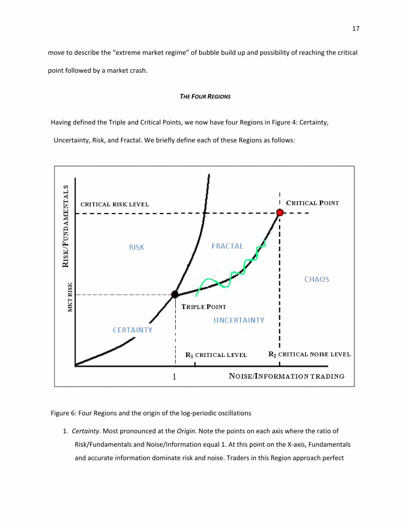
Having defined the Triple and Critical Points, we now have four Regions in Figure 4: Certainty,
Uncertainty, Risk, and Fractal. We briefly define each of these Regions as follows:
Figure 6: Four Regions and the origin of the log‐periodic oscillations
1. Certainty. Most pronounced at the Origin. Note the points on each axis where the ratio of
Risk/Fundamentals and Noise/Information equal 1. At this point on the X‐axis, Fundamentals
and accurate information dominate risk and noise. Traders in this Region approach perfect

18
information as the two ratios go to zero—when traders have perfect information about the
fundamental value of a firm.
2. Uncertainty. To the right of the Triple Point location on the X‐axis, traders lose contact with any
reliable means of attaching true value to information about a particular stock/firm. This results
in Noisy information, as traders guess one way or another. Uncertainty peaks at the location of
the Critical Point on the X‐axis.
3. Risk. Above the location of the Triple Point on the Y‐axis, traders move away from simply trading
based on knowledge about the current “fundamental” value of a stock/firm to start betting on
future value. Risk increases up to the location of the Critical Point on the y‐axis. Above this
point we show “Chaotic Risk;” this is the point where risk‐taking becomes vulnerable to
chaos—bifurcations that can set off significant crashes.
Note that we show Knight’s (1921) risk, uncertainty, and certainty are juxtaposed at the Triple Point.
This is the core explanation underlying EMH—traders leaning toward all three situations trade
concurrently with quick adjustments of the market shifting toward one or the other of the three
conditions.
4. Fractal. The Region between the Triple and Critical Points is notable for increasingly dramatic
volatility incidents. Since there is growing evidence that many of these incidents follow fractal
patterns, we label the region Fractal, even though there undoubtedly is non‐fractal volatility
present as well.

19
V. NONLINEARITIES BETWEEN TRIPLE AND CRITICAL POINTS
SCALABILITY AND SCALE‐FREE THEORIES
To begin, we recognize three basic Phases in the development of complexity science.
Phase 1 emphasizes critical values and dissipative structures. Is based on the works of Prigogine
(1955, 1984, 1997), Haken (1977, 2004), and Mainzer (1994/2007), among many others. It begins with
the Bénard (1901) process—an energy differential is set up between warmer and cooler surfaces of a
container (measured as temperature, ΔT). In between the 1st and 2nd critical values (Rc1, Rc2), a region
is created where the system undergoes a dramatic shift in the nature of fluid flow. For example,
increasing the heat under water molecules in a vessel exposed to colder air above leads to geometric
patterns of hotter and colder water—the chef’s “rolling boil” emerges; new order appears. The critical
values define the “melting” zone (Kauffman, 1993; Stauffer, 1987), within which new structures
spontaneously emerge; Prigogine (1955) termed these “dissipative structures” because they are
pockets of order—governed by the 1st Law of Thermodynamics—that speed up the dissipation of the
imposed energy toward randomness and entropy according to the 2nd Law (Swenson 1989).
Phase 2 emphasizes agent self‐organization absent outside influence. It consists largely of scholars
associated with the Santa Fe Institute (Pines, 1988; Arrow et al., 1988; Cowan et al., 1994; Arthur et
al., 1997). While Phase 1 focuses mostly on dramatic phase transitions at Rc1,—the edge of order,
Phase 2 complexity scientists focus mostly on Rc2—the “edge of chaos” (Lewin, 1992; Kauffman, 1993).
Focusing on living systems (Gell‐Mann, 2002), Phase 2 emphasizes the spontaneous co‐evolution of
entities (i.e., the agents) in a CAS. Agents restructure themselves continuously, leading to new forms
of emergent order consisting of patterns of evolved agent attributes and hierarchical structures
displaying both upward and downward causal influences. Bak (1996) extends this treatment in his
discovery of “self‐organized criticality”, a process in which small initial events can lead to complexity
cascades of avalanche proportions best described as an inverse power law. The signature elements

20
within the melting zone are self‐organization, emergence and nonlinearity. Kauffman’s “spontaneous
order creation” begins when three elements are present: (1) heterogeneous agents; (2) connections
among them; and (3) motives to connect —such as mating, improved fitness, performance, learning,
etc. Remove any one element and nothing happens. According to Holland (2002) we recognize
emergent phenomena as multiple level hierarchies, bottom‐up and top‐down causal effects, and
nonlinearities. Nonlinearity often stems from scalability reflected as power laws.
Phase 3, Econophysics, is the most recent development. Its focus is on how order creation actually
unfolds once the forces of emergent order creation by self‐organizing agents—such as biomolecules,
organisms, people, or social systems—are set in motion. Key parts of this third phase are fractal
structures, power laws, and scale‐free theory. In his opening remarks at the founding of the Santa Fe
Institute, Gell‐Mann (1988) emphasized the search for scale‐free theories—simple ideas that explain
complex, multi‐level phenomena. Brock (2000) goes so far as to say that “scalability” is the core of the
Santa Fe vision—no matter what the scale of measurement, the phenomena appear the same and
result from the same causal dynamics. Gell‐Mann (2002) concludes his chapter, ” What is
Complexity?” with a focus on scalability.
Fractals and power laws. Consider the cauliflower. Cut off a “floret”; cut a smaller floret from the
first floret; then an even smaller one; and then even another, and so on. Despite increasingly small
size, each lower‐level component performs the same function and has roughly the same design as the
floret above and below it in size. This feature defines it as fractal. Fractals can result from
mathematical formulas—the very colorful ones figuring in Mandelbrot’s “Fractal Geometry” (1982).
We are more interested in fractal structures that stem from adaptive processes—like the cauliflower—
in biological and social contexts. In fractal structures the same adaptation dynamics appear at multiple
levels.

21
The econophysicist Barabási (2002) connects scalability, fractal structure, and power law findings to
social networks. He shows how networks in the physical, biological and social worlds, are fractally
structured such that there is a “rank/frequency” effect—an underlying Pareto distribution showing
many sparsely connected nodes at one end and one very well connected node at the other. If plotted
on a double‐log graph, the Pareto‐distributed progression of increasing numbers of connections from,
say, small airports to giant ones like Heathrow and Atlanta, appears as a negatively‐sloping straight
line. This is the now famous power law “signature” dating back to Auerbach (1913) and Zipf (1949).
Andriani and McKelvey (forthcoming) list 84 kinds of power laws—which are good indicators of fractal
geometry—in social, and organizational phenomena. Stanley et al. (1996) find that manufacturing
firms in the U.S. show a fractal structure, as does Axtell (2001). See also Newman (2005), Newman et
al. (2006), and Clauset et al. (2007).
Scalefree theories explain why fractals appear as they do and behave as they do. Though
scalability may have been at the core of the Santa Fe vision, scale‐free theories have only recently
begun to be consolidated and featured collectively by the econophysicists (West & Deering, 1995;
Mantegna & Stanley, 2000; Newman, 2005). The key feature that sets scale‐free theories apart
from most social science theories is that they use a single cause to explain fractal dynamics at
multiple levels. The earliest dates back to 1638—Galileo’s SquareCube Law; the cauliflower keeps
subdividing to keep its surface area at a constant ratio to its growing volume. Explanations for
why some structures have adaptive success while others do not, range from biology to social
science. If the same theory or principle applies to microbes and to organizations, it is assuredly
scale‐free. Andriani and McKelvey (forthcoming) describe 15 scale‐free theories applying to firms.
At the end of each of the following sections, we add in descriptions quoted from the Andriani and
McKelvey (forcoming) article applying scale‐free theories to management and organizational
research. We also comment on how they explain various kinds of trading behaviors.
THE CHARTISTS

22
Two studies, in particular, support the potential for the existence of co‐operative behavior and
increased number of noise traders to move the system to complex dynamics. Sethi's (1996) model
shows local instability is possible if the adjustment of prices is rapid, chartist demand is highly sensitive
to changes in expectations and the share of wealth in chartist hands is sufficiently large. In contrast, a
unique equilibrium is formed when prices are equal to fundamental values and stability of price
dynamics ensues when the chartist share of market wealth is sufficiently small. In another study, Corcos
et al (2002), placed chartists into a simple model of repetitive interaction that led to hyperbolic bubbles,
crashes and chaos. In this model a typical bubble starts at an exponential growth rate, crosses to non‐
linear power law leading to finite time singularity.
The market may thus move away from the attracting basin and tend toward extreme events when
noise trading exceeds information trading. 'Noise' traders (including chartists) trade from misperceived
information or for idiosyncratic reasons (e.g. liquidity). Black (1986) considers noise essential to the
liquidity of financial markets. It is not reasonable to assume that differences in beliefs about prices are
only the result of different information; noise is even produced by small events and the agents
themselves. Noise trading is trading on noise as if it were information. Heiner (1983) argues that the
difficulty involved in making an optimizing decision under conditions of complex dynamics leads to rule‐
governed behavior (e.g. technical analysis).
The above evidence explains how, under certain circumstances, noise trading in the market
increases, breaks the symmetry in demand /supply and destabilizes prices. Below the first critical value
(R1 in Figure 3), the demand is roughly zero, neither buying nor selling predominates, which agrees with
the dynamic stability in the basin of attraction. Above this critical noise level, two most probable values
emerge that are symmetrical around zero demand as Plerou et al. (2003) describe the bi‐modal
distribution of demand above the first critical level of noise. Sethi (1996) shows that a large fraction of
chartists tends to destabilize prices and can cause attracting periodic orbits to arise. The bimodal

23
distribution of demand reported by Plerou et al. (2003) may suggest oscillation of the market between
negative and positive demand phases. The phase transition at this point is related to abrupt changes in
the trading volume. The reversal frequency of the market sentiment is related to the increasing hazard
rate of crash producing log periodicity in the oscillations. In the bubble build up, rational traders
evaluate the increased hazard rate and adapt their speculative strategy. Sornette (2003) describes the
build‐up of cooperative speculation, which often translates into an accelerating rise of the market.
The following scale‐free theories seem to fit the Chartists best.
Table 1: Scale Free Theories Explaining Nonlinear Trader Behaviors*
Phase transition Turbulent flows: Exogenous energy impositions cause autocatalytic, interaction effects and percolation transitions at a specific energy level—the 1st critical value—such that new interaction groupings form with a Pareto distribution (Prigogine, 1955; Nicolis & Prigogine, 1989).
Contagion bursts
Epidemics; idea contagion: Often, viruses are spread exponentially—each person coughs upon two others and the network expands geometrically. But, changing rates of contagious flow of viruses, stories, and metaphors, because of changing settings such as almost empty or very crowded rooms and airplanes, result in bursts of contagion or spreading via increased interactions; these avalanches result in the power-law signature (Watts, 2003; Baskin, 2005) due to the small-world structures of the underlying networks.
* Material in this and the following Tables quoted from Table 2 in Andriani and McKelvey (forthcoming).
Since our text uses the “critical value” phrase (see this and other underlined phrases), it is logical to
suggest that scalability based on autocorrelation effects is present. Furthermore, the combination of
“rule‐governed behavior” and “cooperative speculation” fits the contagion burst theory—traders
develop rules that spread more quickly because traders often communicate within groups, thus
speeding up the rule‐contagion process
HERDING
When consumers act sequentially rather than concurrently, herd‐like behavior can impede the flow
of information and a slight prevalence of public information (e.g. observing others' actions) is then
sufficient to induce agents to ignore their private information and follow in the direction of the crowd.
In this case, movement along the x‐axis in Figure 3 shows increased “noise” trading.
24
According to Avery and Zemsky (1998) under informationally‐efficient prices, herd behavior occurs
when signals are non‐monotonic and risk is multidimensional. In addition, Brunnermeier (2001),
Bikhchandani and Sharma (2000) and Chamley (2004) concluded that herding does not involve violent
price movements except in the most unlikely environments. Park and Sabourian (2006) though, argue
that for financial‐market herding one needs neither non‐monotonic signal nor multidimensionality of
risk. Instead, extreme price movements with herding are possible in variety of situations; herding often
exacerbates price volatility. They require sufficient amount of noise and the existence of a signal with U‐
shaped conditional distribution (both extreme values generate this signal with large probabilities). The
recipients of this signal are more volatile in their decisions, switching from selling to buying and back.
We adopt this explanation for the bubble build up, where herding traders move through the buy/sell
boundary back and forth (see Figure 3), as they believe more in extreme than in moderate values.
Moreover, both types of herding (buy and sell) are possible in the same model if there are more than
one middle type signals. This dynamical model should also examine the conditions when the trader
changes his action to engage in contrarian behavior. While the large amount of noise is required again,
i.e. proportion of information traders is not too large, now the signal with "hill‐shaped" conditional
distribution is necessary.
With respect to herd behavior in efficient markets, Park and Sabourian (2006) and Bikhchandani and
Sharma (2000) suggest that the profit/utility maximizing investor may reverse their planned decision
based on the belief that other investors are acting on information. While they are herding, they increase
the number of noise traders when the price/fundamentals ratio stays the same. DeLong et al (1990)
asserts that rational speculators' early buying triggers positive‐feedback trading, which also increases
the number of speculators. According to Avery and Zemsky (1998), herding in two dimensions of
uncertainty may not distort prices. When the quality of traders' information uncertainty is added
significant mispricing can occur. Therefore a "vertical move" with increase in price/fundamental ratio is

25
presumed. At the critical overpricing and level of noise the bubble bursts resulting in a second order
phase transition (see below).
One obvious scalability fit is “preferential attraction.” Another is “coral growth.”
Table 2: Scale Free Theories Explaining Nonlinear Trader Behaviors
Preferential attachment
Nodes; gravitational attraction: Given newly arriving agents into a system, larger nodes with an enhanced propensity to attract agents will become disproportionately even larger, resulting in the power law signature (Barabási, 2002; Newman, 2005).
Irregularity generated gradients
Coral growth; blockages: Starting with a random, insignificant irregularity, coupled with positive feedback, the initial irregularity starts an autocatalytic process driven by emergent energy gradients, which results in the emergence of a niche. This explains the growth of coral reefs, innovation systems (Turner, 2000, Odling-Smee et al., 2003).
Preferential attachment is a power‐law description of social ties or contacts. Perhaps a couple of
traders begin with a small irregularity and then their group grows—the more followers they have, the
more new ones they get. In the herding process a social network develops in which some traders have
many contacts while other are isolates simply following the herd. This scale‐free theory seems a good fit
to herding. In addition, herding behavior is similar to coral growth; it begins with traders following
insignificant cues and then positive feedback effects set in with the result that volatility increases.
COEVOLUTION
We suggest that breaking through the first critical level of noise the system enters into self‐
organizing dynamics or coevolutionary dynamics. There should be an initiating event such as new
trading rules, hedging techniques, or the development of new derivative products. Individual traders
and institutions engage in these initiating events and in the process of learning and adaptation, the
noise level increases. Maruyama (1963) observes that initiating events may be random and insignificant.
Arthur (1990) focuses on positive feedbacks stemming from initially small instigation events. Casti
(1994) and Brock (2000), by continuing the focus on power laws, present a vision of co‐evolution as a
“driver” of complex system adaptation. McKelvey (2002) outlines the necessary and sufficient conditions
for coevolution to occur. In addition to the initiating events the following four conditions must also exist:
1. Heterogeneous agents (I believe so far we convinced the reader in their existence).

26
2. Adaptive learning abilities
De Long et al. (1990), argue that if rational speculators purchase ahead of noise demand, this may
trigger positive‐feedback trading. An increase in the number of forward‐looking speculators can increase
volatility about fundamentals. Fundamentalists base their decision on the deviation of the asset prices
from fundamentals and chartists on the trends they discern from past observations of the data. Their
interaction is described by the disequilibrium models of Beja and Goldman (1982) and Chiarella (1992).
The first model is linear and instability is global. The second one is a nonlinear version and prices
oscillate around but never converge to fundamentals. The model agrees with the assertion of DeLong et
al. (1990) that unboundedly rational traders take full account of the presence of noise traders, and
destabilize prices to exploit the adaptive behavior of the latter.
3. Agents are able to interact and influence each other
4. Higher level constraint, adaptation to which motivates the coevolutionary process
The four conditions listed above fit our earlier introduction of self‐organization‐based complexity
theory (see Kauffman, 1993; Holland, 1995, etc.). Several scalability theories fit coevolution.
Table 3: Scale Free Theories Explaining Nonlinear Trader Behaviors
Spontaneous order creation
Heterogeneous agents seeking out other agents to copy/learn from so as to improve fitness generate networks; there is some probability of positive feedback such that some networks become groups, some groups form larger groups & hierarchies (Kauffman, 1993; Holland, 1995).
Least effort Language; transition: Word frequency is a function of ease of usage by both speaker/writer and listener/reader; this gives rise to Zipf’s (power) Law; now found to apply to language, firms, and economies in transition (Zipf, 1949; Ishikawa, 2005; Podobnik et al., 2006)).
The foregoing discussion zeros in on coevolution that is based on positive feedback. The “irregularity
generated ingredients” (coral growth) theory fits here (but we don’t repeat it in Table 3). In addition, the
self‐organization process is at the heart of the “spontaneous order creation” theory. The various studies
listed in support of “least effort” theory suggest that freedom to self‐organize without constraint will
produce power‐law distributed rank/frequency formations—in the foregoing, traders coevolve toward
the most efficient set of trading rules, hedging techniques, derivative products, and so on.
VOLATILITY

27
In the EM paradigm volatility follows Brownian motion (no memory), while long range dependence
(power law in the autocorrelation function) has been detected in financial time series. Research on
the scaling behavior of volatility explains price changes at different horizons—hourly, daily, weekly
monthly and reveals vertical dependence that is explained by the existence of traders with different
time horizons. Coarse volatility at low frequency captures the views and actions of long‐term traders
while fine volatility at high frequency captures the views and actions of short‐term traders. It has been
shown in Müller et al. (1997) and Dacorogna et al. (2001) that there is an asymmetry in that coarse
volatility predicts fine volatility better than the other way around.
Gençay and Selçuk (2004) show that in such heterogeneous markets, low‐frequency shocks
penetrate though all layers to the short‐term traders, while high frequency shocks appear to be
short lived. This explains the patterns of volatility observed in endogenous shocks as a result of self‐
organization (i.e., underlying chaotic dynamics—i.e., the period doubling, bifurcation state). Here also
belongs the latest Sornette et al. (2002) article pointing to the cumulative effect of small shocks.
The following scale‐free theories explain volatility best.
Table 4: Scale Free Theories Explaining Nonlinear Trader Behaviors
Self-organized criticality
Sandpiles; forests; heartbeats: Under constant tension of some kind (gravity, ecological balance, delivery of oxygen), some systems reach a critical state where they maintain adaptive stasis by preservative behaviors—such as sand avalanches, forest fires, changing heartbeat rate, species adaptation—which vary in size of effect according to a power law (Bak, 1996).
Interacting fractals
Food web; firm & industry size: The fractal structure of a species is based on the food web (S. Pimm quoted in Lewin 1992, p. 121), which is a function of the fractal structure of predators and niche resources (Preston, 1948; Pimm, 1982; Solé et al., 2001; West, 2006).
Volatility is simply prices changes that range from many small movements to a few large movements,
with a crash being the largest. This process is exactly what Bak (1996) emphasizes in his “self‐organized
criticality” theory—the many small to few large change movements that keep the slope of a sandpile at
a certain angle, are seen in all sorts of processes whereby a particular functionally adaptive position is
maintained—sandpiles, species, markets, and so on. Since we know that U.S. manufacturing firms, for
example, are power‐law distributed, and that many industries are as well (Andriani and McKelvey,

28
forthcoming) the valuation basis of trading behavior occurs in the context of interacting fractal
structures, such that the “predator‐prey” relationships (otherwise called M&A and other competitive
activites) underly the multifractal volatility incidents we see in market behavior.
VI. CONCLUSION
Under the efficient market paradigm, rational investors find undervalued stocks to buy and for the
most part will exercise a buy and hold strategy. There will be very little trading in the undervalued zone
because of a lack of supply at this price as traders would only sell in case of liquidity need. The price
quickly adjusts to its fair value—i.e., around the Triple Point—where the coexistence of the three
phases keeps normally functioning market in the basin of attraction. At this point fair value prevails,
noise trading equals information trading and the average net demand is 0. At this level we have very
simple rules, information is shared and investors are rational with unlimited abilities to process
information. The market quickly adjusts to new information, anomalies are short lived and noise levels
are low. We see this as the juxtaposition and rapid oscillation among Knight’s (1921) elements of risk,
uncertainty, and certainty. Under these conditions, linear models will provide appropriate
approximations. EMH also states that it is not possible to beat the market, since arbitrage opportunities
are short lived and any anomalies are randomly distributed. Net demand is zero and the distribution of
orders is symmetric around zero.
In reality, of course, institutions and individual investors, in an attempt to beat the market, introduce
hedging strategies, trading rules, derivative securities, etc. and the complexity of the financial trading
system increases. As complexity rises, heterogeneous agents switch increasingly from information
trading to rule‐governed behavior such that the ratio of noise traders to information trader increases. It
has been shown that increased noise in the market leads to bimodal net demand distribution
(bifurcation) and the buildup of bubbles. Bubbles are built when noise‐ and risk‐based trading increases

29
as a result of an initiating event and the market moves away from the basin of attraction. However, the
market may restore to the Triple Point (soft landing) or reach the Critical Point when the bubble bursts.
We suggest a number of scale‐free theories assembled by Andriani and McKelvey (forthcoming) to
explain the various trader‐behaviors that serve to move trading behaviors from the Triple Point to,
perhaps, the Critical Point. All of these serve to reduce trader heterogeneity. We know from LeBaron ‘s
(2005) computational model that loss of heterogeneity results in market crashes. Since all of the scale‐
free theories explain Pareto‐distributed, or in other words, power‐law distributed, our contribution is to
offer explanations for the various power‐law distributed and multifractal volatility distributions that
Sornette (2003 a,b), Sornette et al. (1996;2002), Sornette and Johansen(1998, 2001), Johansen, et
al.(2000) and others find occurring between the Triple and Critical Points.
With the increase of noise trading, prices destabilize and periodic orbits emerge as demand
distribution bifurcates. The boundary between buy and sell states is crossed multiple times forming log
periodic oscillations in the price. Coevolution of trading rules towards one super rule (Lebaron, 2001)
leads to order in the market as all traders adopt the same decision and the market collapses (Johansen
and Sornette, 1997).
REFERENCES
Adler, R., R. Feldman, and M. Taqqu. 1998. A Practical Guide to Heavy Tails: Statistical Techniques and
Applications. Basel, Switzerland: Birkhäuser.
Andriani, P., and B. McKelvey. 2007, “Beyond Gaussian Averages: Redirecting Organization Science Toward
Extreme Events and Power Laws.” Journal of International Business Studies, 38(7): 1212–1230.
Andriani, P., and B. McKelvey. Forthcoming. “Extremes & Scale‐Free Dynamics in Organization Science: Some
Theory, Research, Statistics, and Power Law Implications.” Organization Science.
Arthur, W. B. 1990. “Positive feedback in the economy.” Scientific American, 262:2; 92–9.
Arthur, W. B., S. N. Durlauf, and D. A. Lane, eds. 1997. The Economy as an Evolving Complex System.
Proceedings of the Santa Fe Institute, Vol. XXVII, Addison‐Wesley, Reading, MA.
Auerbach, F. 1913. “Das Gesetz der Bevolkerungskoncentration.” Petermanns Geographische Mitteilungen 59:
74–6.
Axtell, R. L. 2001. “Zipf distribution of U.S. firm sizes.” Science 293: 1818–1820.

30
Bak, P. 1996. How Nature Works: The Science of Selforganized Criticality. New York: Copernicus.
Banerjee, A. V. 1992. "A Simple Model of Herd Behavior." The Quarterly Journal of Economics 107: 797–817.
Barabási, A.‐L. 2002. Linked: The New Science of Networks, Cambridge, MA: Perseus.
Baskin, K. 2005. “Complexity, stories and knowing.” Emergence: Complexity & Organisation 7: 32–40.
Baum, J. A. C., and B. McKelvey. 2006. “Analysis of Extremes in Management Studies.” Pp. 123–196 in Research
Methodology in Strategy and Management, Vol. 3. Elsevier Ltd.
Bikhchandani, S., D. Hirshleifer, and I. Welch. 1992. “A Theory of Fads, Fashion, Custom, and Cultural Change
as Informational Cascades.” Journal of Political Economy 100: 992–1026.
Black, F. 1972. “Capital Market Equilibrium with Restricted Borrowing.” Journal of Business 45: 444–455.
Black, F. and M. Scholes 1973. “The Pricing of Options and Corporate Liabilities.” Journal of Political Economy
81: 637–654.
Black, F. 1986. “Noise.” Journal of Finance 41: 529–543.
Breymann, W., S. Ghashghaie, and P. Talkner 2000. “A Stochastic Cascade Model for FX Dynamics.”
International Journal of Theoretical and Applied Finance 3:3: 357–360.
Brock, W. A. and C. H. Hommes. 1998. “Heterogeneous beliefs and routes to chaos in a simple asset pricing
model.” Journal of Economic Dynamics and Control 22:(8–9): 1235–1274.
Brock, W. A., C. Hommes, and F. Wagener. 2005. “Evolutionary Dynamics in Markets with Many Trader
Types.” Journal of Mathematical Economics 41: 7–42.
Brock, W. A. 2000. “Some Santa Fe scenery.” Pp. 29–49 in The Complexity Vision and the Teaching of
Economics, ed. D. Colander. Edward Elgar, Cheltenham, UK, pp. 29–49.
Brown, S., L., and K. M. Eisenhardt. 1998. Competing at the Edge: Strategy as Structural Chaos. Boston, MA:
Harvard Business School Press.
Brunnermeier, M. K. 2001. Asset Pricing under Asymmetric Information : Bubbles, Crashes, Technical Analysis,
and Herding. Oxford, UK: Oxford University Press.
Calvet, L., A. Fisher, and B. Mandelbrot 1997. “A Multifractal Model of Asset Returns, Working Paper, Yale
University.
Calvet, L. E., and A. J. Fisher 2008. Multifractal Volatility: Theory, Forecasting, and Pricing. Burlington, MA:
Academic Press.
Casti, J. L. 1997. WouldBe Worlds: How Simulation Is Changing the Frontiers of Science. New York: Wiley.
Chiarella, C. 1992. “Developments in Nonlinear Economic Dynamics: Past, Present & Future. In H. Hanusch,
ed., Die Zukunft der Okonomischen Wissenschaft. Verlag Wirtschaft und Finanzen.
Chiarella, C., Dieci, R., and L. Gardini 2002. “Price Dynamics and Diversification under Heterogeneous
Expectations.” Computing in Economics and Finance 88: Society for Computational Economics.

31
Clauset, A., C. R. Shalizi, and M. E. J. Newman. 2007. “Power‐law Distributions in Empirical Data.”
ArXiv:0706.1062v1 [physics.data‐an] June.
Corcos, A., J‐P Eckmann, A Malaspinas, Y Malevergne, and D Sornette, 2002. “Imitation and contrarian
behaviour: hyperbolic bubbles, crashes and chaos.” Quantitative Finance 2: 264–281.
Cowan, G. A., D. Pines, and D. Meltzer. 1994. Complexity: Metaphors, Models, and Reality. Reading, MA:
Addison‐Wesley.
Dacorogna, M., R. Gençay, U. Müller, O. Pictet, and R. Olsen 2001. An Introduction to HighFrequency Finance.
San Diego: Academic Press.
De Long; J. B, A. Shleifer; L. H. Summers, and R. J. Waldmann. 1990. “Positive Feedback Investment Strategies
and Destabilizing Rational Speculation.” The Journal of Finance 45:2: 379–395.
Fama, E. F. 1965. “Random Walks in Stock Market Prices.” Financial Analysts Journal 21(5): 55–59.
Gaunersdorfer, A. 2000. “Adaptive beliefs and the volatility of asset prices.” Technical report, SFB Adaptive
Information Systems and Modeling in Economics and Management Science.
Gaunersdorfer, A. 2000a. “Endogenous fluctuations in a simple asset pricing model with heterogeneous
agents.” Journal of Economic Dynamics and Control 24:(5–7): 799–831.
Gell‐Mann, M. 1988. “The concept of the Institute.” Pp. 1–15 in D. Pines, ed. Emerging Synthesis in Science.
Boston, MA: Addison‐Wesley.
Gell‐Mann, M. 2002. “What is complexity?” Pp. 13–24 in A. Q. Curzio, and M. Fortis, eds., Complexity and
Industrial Clusters, Heidelberg, Germany: Physica‐Verlag.
Gençay, R., and F. Selçuk. 2004. “Asymmetry of Information Flow between Volatilities across Time Scales.” No
90, Econometric Society 2004 North American Winter Meetings
Haken, H. 1977. Synergetics: An Introduction, Berlin Germany: Springer‐Verlag.
Haken, H. 2004. Synergetics: Introduction and Advanced Topics. Berlin: Springer‐Verlag.
Heiner, R. 1983. “The origin of predictable behaivior.” American Economic Review 73: 560–595.
Holland, J. H. 1995. Hidden Order: How Adaptation Builds Complexity, Reading, MA: Addison‐Wesley.
Holland, J. H. 2002. “Complex adaptive systems and spontaneous emergence.” Pp. 25–34 in A. Q. Curzio, and
M. Fortis, eds., Complexity and Industrial Clusters. Heidelberg, Germany: Physica‐Verlag.
Ishikawa, A. 2006. “Pareto index induced from the scale of companies.” Physica A 363:2: 367–76.
Johansen, A., O. Ledoit, and D. Sornette. 2000. “Crashes as critical points.” International Journal of Theoretical
and Applied Finance 3:2: 219–255.
Johansen, A.; Sornette. D, 1998. “Stock market crashes are outliers.” The European Physical Journal B, pp. 141–
143.
Johansen, A., and D. Sornette, D. 1999. “Modeling the stock market prior to large crashes.” The European
Physical Journal B, pp. 167–174.

32
Jondeau, E., S.‐H. Poon, and M. Rockinger. 2007. Financial Modeling under NonGaussian Distributions. London:
Springer‐Verlag.
Kauffman, S. A. 1993. The Origins of Order. New York: Oxford University Press.
Kiyono, K., Struzik, R. Zbigniew, Y. Yamamoto. 2006. “Criticality and Phase Transition in Stock‐Price
Fluctuations.” Physical Review Letters 96:6: id. 068701
Knight, F. H. 1921. Risk, Uncertainty, and Profit. Boston: Houghton Mifflin.
LeBaron, B. 2001. “ Volatility Magnification and Persistence in an Agent Based Financial Market.” Working
paper, Brandeis University.
LeBaron, B. 2005. “Agent‐based Computational Finance.” Working paper, Brandeis University.
Lewin, R. 1992. Complexity: Life at the Edge of Chaos. Chicago, IL: University of Chicago Press [2nd ed. 1999.]
Lillo, F., and J. D. Farmer 2005. “The Key Role of Liquidity Fluctuations in Determining Large Price
Fluctuations.” Fluctuations and Noise Lett. 5: L209–L216.
Lintner, J. 1965. “The Valuation of Risk Assets and the Selection of Risky Investments in Stock Portfolios and
Capital Budgets.” Review of Economics and Statistics 47: 13–37.
Lovejoy, S., D. Schertzer 1999) Stochastic chaos, symmetry and scale invariance, ECO‐TEC: Architecture of the
In‐between, edited by Amerigo Marras, Storefront Book series, copublished with Princeton Architectural
Press, 80–99.
Lux, T. 1995. Herd behavior, bubbles and crashes. Economic Journal, 105, 881–896.
Lux, T. 1998. The socio‐economic dynamics of speculative markets: interacting agents, chaos and the fat tails
of return distributions. Journal of Economic Behavior and Organization, 33, 143–165.
Mainzer, K. 1994. Thinking in Complexity: The Complex Dynamics of Matter, Mind, and Mankind. Springer‐
Verlag, New York. [5th ed. 2007.]
Malevergne, Y., and D. Sornette 2005. Extreme Financial Risks: From Dependence to Risk Management. London:
Springer‐Verlag
Mandelbrot, B.B. 1963. “The Variation of Certain Speculative Prices.” Journal of business 36: 394–419.
Mandelbrot, B.B. 1970. “Long‐run Interdependence in Price Records and Other Economic Time Series.”
Econometrica 38: 122–123.
Mandelbrot, B.B. 1982. The Fractal Geometry of Nature. New York: Freeman.
Mandelbrot, B. 1997) “Fractals and Scaling in Finance, Discontinuity, Concentration Risk.” New York:
Springer‐Verlag.
Mandelbrot, B. 2001. “Scaling in financial prices: III. Cartoon Brownian motions in multifractal time.”
Quantitative Finance. 1:4; 427–440.

33
Mandelbrot, B., and R. L. Hudson. 2004. The (mis)Behavior of Markets: A Fractal View of Risk, Ruin, and
Reward. New York: Basic Books.
Mandelbrot, B. B. 1963. “The variation of certain speculative prices.” Journal of Business 36: 394–419.
Mandelbrot, B. B. 1999. “A Fractal Walk Down Wall Street.” Scientific American 280:2: 70–73.
Mandelbrot, B. B., A .J. Fisher, and L. E. Calvet. 1997. “A Multifractal Model of Asset Returns.” Cowles
Foundation Discussion Paper # 1164, Sauder School of Business, University of British Columbia, CA.
Mantegna, R. N., and H. E. Stanley. 1995. “Scaling Behavior of an Economic Index.” Nature 376: 46–49.
Mantegna, R. N., and H. E. Stanley. 2000. An Introduction to Econophysics. Cambridge, UK: Cambridge
University Press.
Maruyama, M. 1963. “The Second Cybernetics: Deviation‐amplifying Mutual Causal Processes.” American
Scientist 51: 164–79.
McKelvey, B. 2004. “Toward a 0th Law of Thermodynamics: Order Creation Complexity Dynamics from
Physics & Biology to Bioeconomics.” Journal of Bioeconomics 6: 65–96.
McKelvey, B., and P. Andriani. 2005. “Why Gaussian statistics are mostly wrong for strategic organization.”
Strategic Organization 3:2: 219–228.
Muller, U., M. Dacarogna, O. Picket, M. Schwarz, and C. Morgenegg, 1990. “Statistical study of foreign exchange
rates, empirical evidence of a price change scaling law, and intraday analysis.” Journal of Banking and
Finance 14: 1189–1208.
Müller, U. A., M. M. Dacorogna, R. D. Dav´e, R. B. Olsen, O. V. Pictet, and J. E. von Weizsäcker. 1997. “Volatilities
of Different Time Resolutions—Analyzing the Dynamics of Market Components.” Journal of Empirical
Finance 4: 213–239.
Muzy, J., J. Delour, and E. Bacry. 2000. “Modeling Fluctuations of Financial Time Series: from Cascade Process
to Stochastic Volatility Model.” European Physics Journal B 17: 537–548.
Newman, M.E.J. 2005. “Power laws, Pareto distributions and Zipf’s law.” Contemporary Physics 46:5: 323–351.
Newman, M., A.‐L. Barabási, and D. J. Watts, Eds. 2006. The Structure and Dynamics of Networks. Princeton, NJ:
Princeton University Press.
Nicolis, G., and I. Prigogine. 1989. Exploring Complexity: An Introduction. New York: Freeman.
Odling‐Smee, F. J., K. N. Laland, and M. W. Feldman. 2003. Niche Construction. Princeton, NJ: Princeton U.
Press.
Peters, E. E. 1991. Chaos and Order in the Capital Markets. New York: Wiley.
Peters, E. E. 1994. Fractal Market Analysis: Applying Chaos Theory to Investment & Economics. New York:
Wiley.
Picket, O. V. et al. 1995. “Statistical Study of Foreign Exchange Rates, Empirical Evidence of a Price Change
Scaling Law and Intraday Analysis.” Journal of Banking and Finance 14: 1189–1208.

34
Pimm, S. L. 1982. Food Webs. Chicago, IL: University of Chicago Press. [2nd ed. 2002.]
Pines, D., ed. 1988. Emerging Syntheses in Science. Proceedings of the Santa Fe Institute, Vol. I, Reading, MA:
Addison‐Wesley.
Plerou, V., P. Gopikrishnan, X. Gabaix, and H. E. Stanley. 2002. “Quantifying Stock‐price Response to Demand
Fluctuations." Physical Review E 66: 027104‐1–4.
Plerou, V., P. Gopikrishnan, and H. E. Stanley. 2003. “Two‐phase Behaviour of Financial Markets.” Nature 421–
130.
Podobnik, B., D. Fu, T. Jagric, I Grosse, and H. E. Stanley. 2006. “Fractionally Integrated Process for Transition
Economics.” Physica A 362:2: 465–70.
Prechter, R. 1999. The Wave Principle of Human Social Behavior: The New Science of Socionomics. Gainesville,
GA: New Classics Library.
Preston, F. W. 1948. “The Commonness, and Rarity, of Species.” Ecology 29: 254–283.
Prigogine, I. 1955. An Introduction to Thermodynamics of Irreversible Processes. Springfield, IL: Thomas.
Prigogine, I., and I. Stengers. 1984. Order Out of Chaos: Man’s New Dialogue with Nature. New York: Bantam.
Prigogine, I. (with I. Stengers). 1997. The End of Certainty: Time, Chaos, and the New Laws of Nature. New
York: Free Press.
Rachev, S. T., and S. P. Mittnik. 2000. Stable Paretian Models in Finance. New York: Wiley.
Rook, L. 2006. “An Economic Psychological Approach to Herd Behavior.” Journal of Economic Issues 40: 75–95.
Rosser, J. B. 2000. From Catastrophe to Chaos: A General Theory of Economic Discontinuities: Mathematics,
Microeconomics, Macroeconomics, and Finance, Vol. 1, (2nd ed.). Norwell, MA: Kluwer.
Rossoa, O. A., A. Figliolaa, S. Blancoa, and P. M. Jacovkis. 2004. “Signal separation with almost periodic
components: a wavelets based method.” Revista Mexicana de Fisica 50:2: 179–186.
Schmitt, F., D. Schertzer, and S. Lovejoy. 1999. “Multiftactal Analysis of Foreign Exchange Data.” Applied
Stochastic Models and Data Analysis 15: 29–55.
Schroeder, M. 1991. Fractals, Chaos, Power Laws. New York: Freeman.
Sharp, W. F. 1964. “Capital Asset Prices: A Theory of Market Equilibrium Under Conditions of Risk.” Journal of
Finance 19: 425–442.
Solé, R. V., D. Alonso, J. Bascompte, and S. C. Manrubia. 2001. “On the Fractal Nature of Ecological and
Macroevolutionary Dynamics.” Fractals 9: 1–16.
Sornette, D. 2003(a). Critical market crashes, Physics reports 378:11, 1–98, Elsevier Science.
Sornette, D. 2003(b). Why Stock Markets Crash? Princeton, NJ: Princeton University Press
Sornette, D. 2004. Critical Phenomena in Natural Sciences: Chaos, Fractals, Self organization and Disorder:
Concepts and Tools (2nd ed.). Berlin: Springer‐Verlag.

35
Sornette, D., and A. Johansen, J.‐P. Bouchaud. 1996. “Stock Market Crashes, Precursors and Replicas.” Journal
Phys. I France 6:January 1996: 167–175.
Sornette, D., and A. Johansen. 1997. “Large Financial Crashes.” Physica A 245:3–4: 411–422.
Sornette, D., and A. Johansen. 1998. “A Hierarchical Model of Financial Crashes Physica A 261:3–4: 581–598
Sornette, D., and A. Johansen. 2001. “Large stock market price drawdowns are outliers”
D. Sornette, D, Y. Malevergne, J.F. Muzy. 2002. Volatility fingerprints of large shocks: endogeneous versus
exogeneous, Risk Mag. (http://arXiv.org/abs/cond‐mat/0204626).
Stanley, M. H. R., L. A. N. Amaral, S. V. Buldyrev, S. Havlin, H. Leschhorn, P. Maass, M. A. Salinger, and H. E.
Stanley. 1996. “Scaling behaviour in the growth of companies.” Nature 379: 804–806.
Stauffer, D., 1987, “On Forcing Functions in Kauffman’s Random Boolean Networks.” Journal of Statistical
Physics 46: 789−794.
Swenson, R., 1989. “Emergent Attractors and the Law of Maximum Entropy Production: Foundations to a
Theory of General Evolution.” Systems Research 6: 187−197.
Tirole, J. 1982. “On the Possibility of Speculation under Rational Expectations.” Econometrica 50: 1163–1181.
Turiel, A., and C. Pérez‐Vicente. 2002. “Multifractal Geometry in Stock Market Time‐Series.” Preprint
submitted to Elsevier Science.
Turner, J. S. 2000. The Extended Organism. Cambridge, MA: Harvard University Press.
Watts, D. 2003. Six Degrees: The Science of a Connected Age. New York: Norton.
Wei, G., M. Zhan, and C.‐H. Lai. 2002. “Tailoring Wavelets for Chaos Control.” Physical Review Letters 89, 28,
284103–1.
West, B. J. 2006. Where Medicine Went Wrong. Singapore: World Scientific.
West, B. J., and B. Deering. 1995. The Lure of Modern Science: Fractal Thinking, Singapore: World Scientific.
Westerhoff, F. H. 2005. “Heterogeneous Traders, Price‐Volume Signals, and Complex Asset Price Dynamics.”
Discrete Dynamics in Nature and Society 1: 19–29.
White, E. N. 1996. Stock Market Crashes and Speculative Manias (International Library of Macroeconomic and
Financial History. Cheltenham, UK: Edward Elgar.
Zipf, G. K. 1949. Human Behavior and the Principle of Least Effort. New York: Harper.