Title

Facing the Challenges of the New European Space of HigherEducation Through Effective Use of Computer AlgebraSystems as an Educational Tool (Computer Algebra Systemsand Education : A Research about Effective Use of CAS inMathematics Education)

Author(s) Iglesias, Andres

Citation 数理解析研究所講究録 (2009), 1624: 114-128

Issue Date 2009-01

URL http://hdl.handle.net/2433/140265

Right

Type Departmental Bulletin Paper

Textversion publisher

Kyoto University

Facing the Challenges of the New EuropeanSpace of Higher Education Through

Effective Use of Computer Algebra Systemsas an Educational Tool

Andr\’es IglesiasDepartment of Applied Mathematics and Comp. Sciences

University of Cantabria, Avda. de los Castross/n, E-39005, Santander, Spain

iglesias@unican.eshttp://personales.unican.es/iglesias

Abstract

Academic institutions of most European countries are now in the midst of theprocess of overall convergence of studies at university level, the so-called EuropeanSpace of Higher Education. This process, bom from Bologna’s declaration, impliesa dramatic change in our way of teaching and learning. This change is speciallychallenging in very difficult subjects such as Mathematics and other scientific dis-ciplines, which typically suffer from high failure rates. It’s author’s opinion thatComputer Algebra Systems are very powerful tools (arguably the best ones) toface the challenges of this new approach to Higher Education. To support suchclaims, some examples of Mathematica packages developed by the author duringthe last few years for teaching different subjects in scientific degrees (accordingto the principles and regulations of the European Space of Higher Education) arebriefly described.

1 IntroductionSince its signature in 1999, Bologna’s Declaration has epitomized the much-needed,largely-demanded process of changes umdertaken in most European countries in orderto reform their Higher Education system. This agreement is not only designed for newcurricula and academic regulations; it also accounts for a new approach to teaching andlearning (in author’s opinion, the most important issue of this process). This challengeis specially important in very difficult subjects such as Mathematics and other scientificdisciplines, which typically suffer from high failure rates. Several academic reports havepointed out the difficulties our students face when studying (and suffering) mathematicalsubjects. Students and professors at university often cite lack of preparation from highschool, poor study habits and the rapid pace of the course as reasons for such low scores.

数理解析研究所講究録第 1624巻 2009年 114-128 114

Right or not, the truth is Mathematics is very much practice-based. Students mayget a concept in the classroom, but they will certainly lose it if not reinforced by home-work. For doing so, students need to be provided with good supporting materials sothat they can effectively leam by themselves. High-quality, helpful educational materialsallow underachieving students catching up on belated assignments and get extra time forsuccessful backtracking. It is at this point where Computer Algebra Systems (CAS on-wards) can really pave the way, making the most with less. In author’s opinion, CAS arevery powerful tools (arguably the best ones) to face the challenges of this new approachto Higher Education. This paper aims at supporting such claims by presenting someexamples of Mathematica packages developed by the author during the last few years forteaching different subjects in scientific degrees according to the principles and regulationsof the European Space of Higher Education.

2 Some Illustrative Examples

2.1 Example 1: Binary Distillation ColumnThis section is about a Mathematica program for distillation column design describedoriginally in [7]. This example is intended for students of Chemical Engineering de-gree who can use a CAS as a useful tool for their symbolic/numerical computations andgraphical output. For the sake of simplicity, we consider the case of continuous distillationcolumms for binary mixtures. However, our approach is very general as it can be appliedto any other kind of distillation columns by simply replacing our assumptions by thoseof each specific case. In this example, we assume that the colunms are designed throughMcCabe-Thiele’s procedure [11, 12]. This is a graphical method which determines thenumber of stages required for the desired degree of separatIon and the location of thefeed tray as functions of some parameters of the problem. The program is general enoughto analyze a number of different mixtures under different conditions as well as the roleof many relevant parameters of this process. To this purpose, an adequate combinationof symbolic and numerical calculations is achieved. From these calculations, both nu-merical and grapluical outputs are obtained. In fact, the graphical output is actually aMathematica movie of McCabe-Thiele’s diagram.

The method has been implemented as a Mathematica package, called MTBDC. $m$ , wherethis acronym stands for McCabe- Riele Binary Mstillation Column. This section de-scribes one example of application of this program to a equimolar $(i.e. x_{f}=0.5)$ binarymixture whose relative volatility is $\alpha=4$ . Our target is to design a distillation columnthat obtains a destillate with 85 % of purity $(i.e. x_{d}=0.85)$ and bottoms with 5 % ofpurity $(i.e. x_{b}=0.05)$ . The first comand Reflux [xd, xf $l$ alpha] determines three values:the reflux, and the liquid and vapor compositions of the more volatile component:

In [1] $:=$ Needs $[^{1t}MCBDC$ ‘ $||]$

In [2] $:=$ Reflux [0.85, 0.5,4]Out[2] $:=\{1.75,0.2,0.5\}$

Then, the command OperatingLines [xd, xf, alpha] is applied to the calculation ofthe operating lines of the rectification section and the stripping section, shown in Fig.l(d). The third step is to apply McCabe-Thiele’s method to determine the number of

115

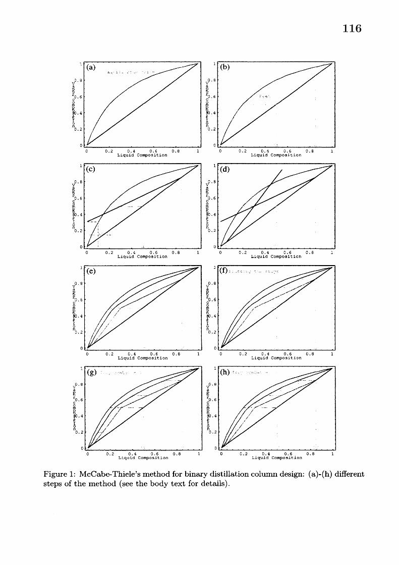
Figure 1: McCabe-Thiele’s method for binary distillation column design: $(a)-(h)$ differentsteps of the method (see the body text for details).

116

Figure 2: McCabe-Thiele’s method for an equimolar heptane-octane mixture with $x_{d}=$

0.98, $x_{f}=0.5,$ $x_{b}=0.05$ and $\alpha=2.17$: (left) $E_{f}=1$ ; (right) $E_{f}=0.65$ .

trays of the column as well as the location of the feed tray. To this end, we define theMTPlot command, which accepts five different arguments, namely, $x_{d},$ $x_{f},$ $x_{b},$ $\alpha$ and theefficiency $E_{f}$ . For example, MTPlot [0.85,0.5,0.05,4,0.6] returns a sequence of 49frames corresponding to the different steps of McCabe-Thiele’s method. Eight of theseframes are displayed in Figure 1.

One of the most remarkable Mathematica features in this work is the possibility togenerate $Q\dot{m}ckTime^{TM}$ movies. For example, the different images in Figure 1 correspondto eight frames of a QuickTime movie that reproduces McCabe-Thiele’s method in agraphical way. The movie is automatically generated from the MTPlot command. Dif-ferent values of its arguments are associated with different initial mixtures and$/or$ finalproducts. This option is specially valuable for educational and training purposes, as wecan obtain a virtually unlimited set of distillation columns in a fast and simple way.

McCabe-Thiele’s method does not allow us to determine all relevant distillation col-umn parameters and thus, some additional equations must also be considered. Thediscussion is beyond the scope of this paper and will not be included here. At this time itis enough to say that a number of different Mathematica commands incorporating theseadditional equations have been implemented in the MTBDC. $m$ package. For example, if westart with an equimolar mixture of heptane-octane with a relative volatility $\alpha=2.17$ andefficiency $E_{f}=1$ and we wish to obtain a destillate with 98 % of heptme and bottomswith only a 5% of heptane, the column parameters can be determined as:

In [3] : $r$ ColumnParameters $[0.98,0.05,0.5,2.17,1]$$Out[3J:=Number$ of trays $=14$ (rebolier included)

Number of Feed $tray=9$Column height $=8.4$ metersDistance between trays $=0.6$ meters

Figure 2 shows the McCabe-Thiele’s diagram of the column for total efficiency $E_{f}=1$

(left) and when the efficiency of the process is only a 65 %, that is $E_{f}=0.65$ (right).In the first case, the column has only 14 trays and its height is 8.4 meters, while in thesecond case the number of trays increases up to 22 and the column height is now 13.2meters.

117

2.2 Example 2: Solving Inequalities

Solving inequalities is a very important topic in Mathematics, with outstanding applica-tions in many areas of theoretical and applied science. Inequalities play a key role becausemany problems cannot be completely and accurately described by using only equalities.However, since there is not a general methodolody for solving inequalities, their sym-bolic computation is still a challenging problem in computational algebra. Depending onthe kind of functions involved, there are many “specialized” methods such as cylindricalalgebraic decomposition, Gr\"oebner basis, quantifier elimination, etc. [1, 6, 8, 13].

This section uses a nonstandard Mathematica package [9], InequationPlot, for dis-playing the two-dimensional solution sets of several inequalities. In particular, it extendsMathematica’s capabilities by providing graphical solutions to many inequalities (suchas those involving trigonometric, exponential and logarithmmic functions) that cannot besolved by using the standard Mathematica commands and packages [14, 15]. The packagealso deals with inequalities involving complex variables by displaying the correspondingsolutions on the complex plane.

Inequalities involving trigonometric functions cannot be solved by standard Mathe-matica commands. For example, let us try to display the solution sets of each of theinequalities

$sin(x+y)> \frac{1}{2}$ (1)

and$sin(2x)+cos(3y)<1$ (2)

on the set $[$ -8, $8]\cross[-8,8]$ by using the standard Mathematica commands. In this case,we must use the command InequalityPlot of the Mathematica package:In [41 $:=<<Graphi$ cs‘ InequalityGraphics

Unfortunately, since the region defined by inequality (1) on the prescribed domain cannotbe broken down into cylinders, Mathematica fails to give the solution:In [5] $:=InequalityPlot$ $[$Sin $[x+y]>1/2,$ $\{x,$ $-8,8\},$ $\{y,$ $-8,8\}]$

Out[5]: $=InequalityPlot:$ : region:The region defined by $sin(x+y)>1/2\wedge-8<=x<=8\wedge-8<=y<=8$ could not bebroken down into cylinders.

On the contrary, the previous inequalities can be solved by loading our package:

In [6] $:=<<$InequationPlot‘which includes the commandInequat $i$ onPlot [ineqs, $\{x$ , xmin, xmax}, $\{y$ , ymin, ymax}, opts]

for displaying the two-dimensional region of the set of points satisfying the inequalitiesineqs of real numbers inside the square [xmin, xmax] $\cross[ymin$ , ymax$]$ . For example,inequalities (1)$-(2)$ can be solved as follows:

In [7] $:=InequationPlot$ [$*,$ $\{x,-8,8\},$ $\{y,-8,8\}$ , AspectRatio-$>Automat$ ic]& /@

$\{Sin[x+y]>1/2$ ,Sin $[$2 $x]+Cos[3y]<1\}$

$Outf7J:=See$ Figure 3

118

$\infty\inftyarrow$$\sim\lrcorner-$ $\}-$

$-$

$-$

$l$

$-$$(\sim$

$\epsilon\}- \mathfrak{l}$ $-$ $\sim$

$-$ .

$-\overline{\cdot\prime\epsilon}-\backslash \overline{\epsilon}_{\vee}---1$.

1

– —-$[$

$arrow$ $\sim$

$1$

$\}$

$($

$r\sim$

$\epsilon|$

$r\backslash$ $\nearrow\backslash$

$r\cdot-\backslash$$’rightarrow$

Figure 3: Some examples of inequality solutions on the square [-8, 8] $\cross[-8,8]$ : (left)$sin(x+y)> \frac{1}{2}$ ; (right) $sin(2x)+cos(3y)<1$ .

Similarly, Fig. 4 displays the solution sets of the inequalities $F(x)+F(y)=1$ and$F(x^{2})+F(y^{2})=1$ (where $F$ stands for the floor function) on the squares $[$-4, $4]\cross[-4,4]$

and [-2, 2] $\cross[-2,2]$ , respectively. We would like to remark that the Mathematica com-mand InequalityPlot does not provide any solution for these inequalities either.

Figure 4: Some examples of inequality solutions: (left) floor$(x)+floor(y)=1$ on thesquare $[$-4, $4]\cross[-4,4]$ ; (right) floor$(x^{2})+floor(y^{2})=1$ on the square $[$-2, $2]\cross[-2,2]$ .

The previous command, InequationPlot, can be generalized to inequalities involvingcomplex numbers. The new commandComplexInequationPlot [ineqs, $\{z$ , {Rezmin, Rezmax}, {Imzmin, Imzmax}}, opts]

displays the solution sets of the inequalities ineqs of complex numbers inside the squarein the complex plane given by $[$Rezmin, $Rezmax]\cross[Imzmin$ , Imzmax$]$ . In this case, the

119

functions appearing within the inequalities need to be real-valued functions of a complexargument, $e.g$ . $Abs,$ $Re$ and $Im$. For example:

In [8] $:=ComplexInequationPlot$ [$\#,$ $\{z,$ $\{-2,3\},$ $\{-3,3\}\}$ , AspectRatio- $>$Automatic]&

/@ $\{1<Abs[z^{rightarrow}2-z+1]<4,1<Abs[z^{-}2-2z]/$Abs $[z^{\sim}2+3]$ く 4 $\}$

$Out[ 8\int:=See$ Figure 5

Figure 5: Some examples of inequality solutions for $z=a+b\in \mathbb{C}$ such that $a\in[-2,3]$

and $b\in[-3,3]$ : (left) $1<||z^{2}-z+1||<4$ ; (right) $1< \frac{||z^{2}-2z||}{||z^{2}+3||}<4$ .

$5—–\wedge^{\wedge}----\sim\sim\backslash -\sim;^{\sim}\backslash \vee\neg\sim\sim\backslash$

$1.\sim$

$\vee\backslash \backslash \backslash \backslash \backslash [_{\backslash }\backslash \backslash \backslash \backslash \backslash \llcorner$

$\sim\sim$

$–\wedge--arrow\sim$$\sim_{s}-$

$\ell-\sim\backslash --\sim--\backslash \sim\vee^{\backslash }\cdot\backslash \wedge^{\backslash }\vee^{\backslash }\backslash \sim\backslash \backslash \backslash \sim\backslash \backslash \sim\backslash \backslash \backslash \backslash \backslash 1_{\backslash }^{\backslash }\backslash \backslash \backslash \backslash \backslash \backslash$

$\sim\sim\sim$$\backslash f^{\mathfrak{l}}\backslash \backslash \backslash \backslash$

$\vee---arrow---\sim-$$\backslash \backslash /\backslash$

$\backslash$

$2_{\backslash }^{-}-\backslash --\sim^{X}’/\sim\backslash \backslash \backslash \sim\backslash _{c}/’\backslash /\backslash /\backslash \backslash \backslash \backslash \backslash \backslash \backslash \backslash \backslash$

$”\nearrow’/$

ノ$\backslash \backslash \backslash$

$\backslash /\backslash$

$0.5$ 1 1. $\lrcorner$

$2_{\lrcorner}$ 3

Figure 6: Solution sets for the inequality systems: (left) Eq. (3); (right) Eq. (4).

The last example shows how complicated the inequality systems can be: in additionto include exponential, logarithmic and trigonometric fimctions, combinations and even

120

compositions of these (and other) functions can also be considered. In Figure 6 thesolutions sets of the inequality systems:

$e^{y} \geq 1\wedge log(x)y\geq 1\wedge x\sqrt{y}<4\wedge x-y>\frac{1}{2}$ (3)

$log(y)\geq_{\tilde{2}}^{1}\wedge sin(x)y\geq x\wedge cos(e^{x-y})\geq 0\wedge sin(x^{2}+y^{2})>0$ (4)

on $[1, 10]\cross[0,10]$ and $[0,3]\cross[1,5]$ respectively are displayed.

2.3 Example 3: Gauss Map of SurfacesThis section focuses on a classical topic in the field of Differential Geometry: the vi-sualization of the Gauss map of a surface. Roughly speaking, the Gauss map projectssurface normals onto a unit sphere, providing a powerful visualization of the geometry ofa graphical object. On the other hand, dynamic visualization of the Gauss map speedsunderstanding of complex surface properties. This section applies a Mathematica pack-age described in [10], GaussMap, for computing and displaying the tangent and normalvector fields and the Gauss map of surfaces described symbolically in either implicit orparametric form. Firstly, we load the package:In [9] $:=<$く DifferentialGeometry‘GaussMap

2.3.1 Implicit Surfaces

The ImplicitNormalField command calculates the normal vector field of any implicitsurface in the form $f(x, y, z)=0$ and retums a graphical output comprised of the surfaceand such a normal vector field. The first example is given by the paraboloid $x^{2}+y^{2}-z=0$ :

In [10] $:=ImplicitNormalField[x^{-}2+y^{\sim}2-z,$ $\{x, -2,2\},$ $\{y, -2,2\},$ $\{z,$ $-1,2\}$ ,Surface-$>Tme$ , PlotPointsSurface-$>\{4,7\}$ , VectorHead- $>Polygon$]

$Out[10]:=See$ Figure 7

Figure 7: The paraboloid $x^{2}+y^{2}-z=0$ and its vector normal field.

121

The ImplicitGaussMap command of an implicit surface returns the original surfaceand its Gauss map on the unit sphere:

In [11] $:=ImplicitGaussMap[x^{\sim}2+y^{\sim}2-z,$ $\{x,$ $-2,2\},$ $\{y,$ $-2,2\},$ $\{z,$ $-1,2\}$ ,PlotPoints- $>\{4,7\}]$

Out $[$ ll $]$ $:=See$ Figure 8

Figure 8: (left) Implicit surface $x^{2}+y^{2}-z=0$ ; (right) its Gauss map.

Next example calculates the normal vector field of the surface $z-x^{2}+y^{2}=0$ :In [12] $:=ImplicitNormalField[z-x^{-}2+y^{\sim}2,$ $\{x, -2,2\},$ $\{y, -2,2\},$ $\{z,$ $-2,2\}$ ,

Surface- $>True$ , PlotPointsSurface- $>\{4,6\}$ , VectorHead-$>Polygon$ ,

PlotPointsNormalField- $>\{3,4\}]$

Out[12]: $=See$ Figure 9

Figure 9: The surface $z-x^{2}+y^{2}=0$ and its vector normal field.

The Gauss map image of such a surface is obtatned as:In [13] $:=ImplicitGaussMap[z-x^{arrow}2+y^{arrow}2,$ $\{x,-2,2\},$ $\{y, -2,2\},$ $\{z,-2,2\}$ ,

PlotPoints-$>\{4,6\}]$

Out[13]: $=See$ Figure 10

122

Figure 10: (left) Implicit surface $z-x^{2}+y^{2}=0$ ; (right) its Gauss map.

A more complicated example is given by the double toms surface, defined implicitly

by $(\sqrt{(\sqrt{x^{2}+y^{2}}-2)^{2}+y^{2}}-2)^{2}+z^{2}-1=0$ and whose normal vector field is shownin Figure 11:

In [14] $:=ImplicitNormalField[$ $($Sqrt $[$ (Sqrt $[x^{-}2+y^{\sim}2]-2$ ) $2+y^{\sim}2]-2)^{\wedge}2+z^{\wedge}2-1$ .$\{x,$ $-6,6\},$ $\{y,-4,4\}_{*}\{z,$ $-1,1\}$ , Surface- $>True$ , VectorHead-$>Polygon$ ,PlotPointsSurface-$>\{5.5\}]$

Out $[$14$]$ $:=See$ Figure11

Figure 11: The double torus surface and its vector normal field.

In [15] $:=ImplicitGaussMap[$ $($ Sqrt $[$ (Sqrt $[x^{\wedge}2+y^{\wedge}2]-2$ ) $2+y^{\text{へ}}2]-2)^{arrow}2+z^{rightarrow}2-1$ ,$\{x,-6,6\},$ $\{y,-4,4\},$ $\{z,-1,1\}$ ,Pl$otPoints->\{5,5\}]$

Out[15]: $=See$ Figure 12It is interesting to remark that, because the Gauss map is a continuous (in fact,

differentiable) function, it is closed for compact sets, i.e. it transforms compact sets into

123

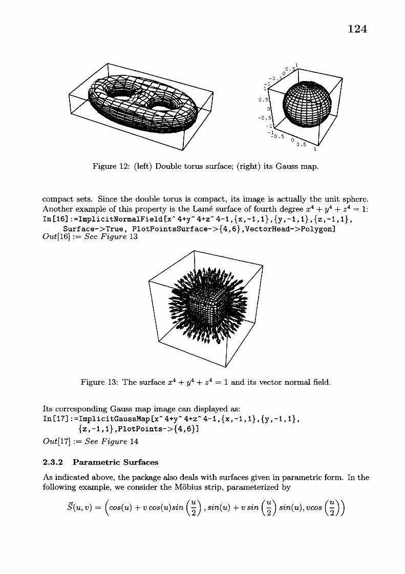
Figure 12: (left) Double torus surface; (right) its Gauss map.

compact sets. Since the double torus is compact, its image is actually the unit sphere.Another example of this property is the Lam\’e surface of fourth degree $x^{4}+y^{4}+z^{4}=1$ :In [16]: $=ImplicitNormalField[x^{\sim}4+y^{arrow}4+z^{-}4-1,\{x,-1,1\},$ $\{y,-1,1\},$ $\{z,-1,1\}$ ,

Surface- $>Tme$ , PlotPointsSurface- $>\{4,6\}$ , VectorHead-$>Polygon$]Out $[$ 16$]:=See$ Figure 13

Figure 13: The surface $x^{4}+y^{4}+z^{4}=1$ and its vector normal field.

Its corresponding Gauss map image can displayed as:In [17] $:=ImplicitGaussMap[x^{rightarrow}4+y^{arrow}4+z^{-}4-1,$ $\{x,-1,1\}$ , $\{y, -1,1\}$ ,

$\{z , -1,1\}$ , PlotPoints-$>\{4.6\}]$

Out $[$ 17$]:=See$ Figure 14

2.3.2 Parametric Surfaces

As indicated above, the package also deals with surfaces given in parametric form. In thefollowing example, we consider the Mobius strip, parameterized by

$\vec{S}(u, v)=(cos(u)+vcos(u)sin(\frac{u}{2}),$ $sin(u)+vsin( \frac{u}{2})sin(u)$ , vcos $( \frac{u}{2}))$

124

Figure 14: Lam\’e surface of fourth degree; (right) its Gauss map.

Figures 15 and 16 show its normal vector field and the Gauss map, respectively.In[18]: $=$ ParametricNormalField $[\{Cos[u]+v$ Cos $[u]$ Sin $[u/2]$ ,

Sin $[u]+v$ Sin $[u/2]$ Sin $[u],v$ Cos $[u/2]\},$ $\{u,$ $0,4$ Pi,Pi/10 $\}$ ,$\{v, -1/2,1/2,0.1\}$ , Surface-$>True$ , PlotPoints- $>\{50,7\}$ ,SurfaceDomain- $>\{\{0,2$ Pi $\},$ $\{-1/2,1/2\}\},VectorHead->Polygon$ ,HeadLength- $>0.25$ , HeadWidth- $>0.1$ , VectorColor-$>RGBColor[1,0,0]]$

$Out[18]:=See$ Figure 15

Figure 15: The M\"obius strip and its vector normal field.

In[19]: $=ParametricGaussMap[\{Cos[u]+v$ Cos $[u]$ Sin $[u/2]$ , Sin $[u]+$$v$ Sin $[u/2]$ Sin $[u],$ $v$ Cos $[u/2]\},$ $\{u,0,4Pi\},$ $\{v$ ,-1/2,1/2$\}$ ,SurfaceDomain- $>\{\{0,2$ Pi $\},$ $\{-1/2,1/2\}\}$ ,PlotPoints$->\{50,7\}]$

$Out[19]:=See$ Figure16

2.4 Example 4: Solving Functional EquationsIn this section we use the Mathematica package FSolve [3, 4], implemented to solvefunctional equations [2, 5]. Let’s start loading the package:In [20] $:=$くく FunctionalEquations‘FSolve‘

125

Figure 16: (left) M\"obius strip surface; (right) its Gauss map.

It includes the command: FSolve [$eqn$ , {functions}, {variables}, options] where $eqn$

denotes the functional equation to be solved, {functions} is the list of unknown functions,{variables} is the list of variables and options allows the users to consider differentdomains for the variables (see Table 1) and classes of feasible functions (see Table 2).

Table 1: List of all feasible domains used in the FSolve package.

For instance, we can calculate the solution of the functional equation $f(x+y)=$

126

Table 2: Classes of feasible fumctions used in the FSolve package.

$g(x)+h(y)$ where $x,$ $y\in \mathbb{R}$ and $f,$ $g,$ $h$ are continuous functions as:In [21] $:=$ FSolve $[f[x+y]==g[x]+h[y],$ $\{f$ , $g,h\},$ $\{x,y\}$ , Domain- $>Real$ ,

Class- $>$Continuous]

Out[21] $:=\{f(x)arrow C(1)x+C(2)+C(3), g(x)arrow C(1)x+C(2), h(x)arrow C(1)x+C(3)\}$

where $C(1),$ $C(2)$ and $C(3)$ are arbitrary constants. Note that a single equation candetermine several unknown functions (such as $f,$ $g$ and $h$ in this example). Note also thatthe solution can depend on one or more arbitrary constants and$/or$ arbitrary functions:In [22] $:=FSolve[f[x]*Sin[y]+h[x]*g[y]==0, \{f , g,h\}, \{x,y\}]$

$\{\{f[x]arrow 0, g[y]arrow C[0]Sin[y]+C[1]Arb[0][y], h[x]arrow 0\}$ ,Out[22]

$:= \{f[x]arrow C[1]Arb[0][x], g[y]arrow-\frac{C[1]Sin[y]}{C[0]}, h[x]arrow C[0]Arb[0][x]\}\}$

In [23] $:=FSolve[k[u]*1[v]==-b[u] , \{k, 1,b\}, \{u,v\}]$

Out[23] $:=$$\{\{k[u]arrow 0, b[u]arrow 0, l[v]arrow C[0]+C[1]*Arb[0][v]\}$ ,$\{k[u]arrow C[0]*Arb[0][u],$ $b[u]arrow C[1]*Arb[0][u],$ $l[v]arrow-(C[1]/C[0])\}\}$ ,

In [24]: $=FSolve[f[g[x]+h[y]]-s[r[x]+s[y]]==0,$ $\{f,g,h.r,$ $s\},$ $\{x,y\}$ ,Domain-$>RealPositive$ , Class-$>Arbitrary$]

Out $[$24$]$ $:=$ $\{\{f[x]arrow s[\frac{x-C|2\rceil-C[3\rceil}{C[1]}],$ $g[x]arrow C[2]+C[1]r[x],$ $h[x]arrow C[3]+C[1]s[x]\}\}$

AcknowledgmentsThis paper is the printed version of an invited talk delivered by the author at RIMS(Research Institute for Mathematical Sciences) workshop on Computer Algebra Systemsand Education; A Research about Effective Use of CAS in Mathematics Education, KyotoUniversity (Japan), August $29th$ . 2008. The author would like to thank the organizersof this exciting RIMS workshop for their diligent work and kind invitation. Specialthanks are owe to Prof. Setsuo Takato (Toho University, Japan) for his friendship, hisgreat support and hospitality and for making my stay in Kyoto such a wonderful andunforgettable experience. It was indeed a lovely time I will never forget. Doomo antgatoogozaimashita! Ookini./

127

This research has been supported by the Computer Science National Program ofthe Spamish Ministry of Education and Science, Project Ref. #TIN2006-13615 and theUniversity of Cantabria.

References[1] Beckenbach, E.F., Bellman, R.E.: An Introduction to Inequalities. Random House,

New York (1961).

[2] Castillo, E., Guti\’errez, J.M., Iglesias, A.: Solving a functional equation. The Mathe-matica Joumal, 5(1) (1995) 82-86.

[3] Castillo, E., Iglesias, A., Cobo, A.: A package for symbolic solutions of fmctionalequations. In: Keranen, V., Mitic, P. (Eds.): Proceedings of the First Intema-tional Mathematica Symposium. Computational Mechanics Publications, $Southam\triangleright$

ton (England), pp. 85-92.

[4] Castillo, E., Iglesias, A.: A package for symbolic solution of real functional equationsof real variables. A equationes Mathematicae, 54 (1997) 181-198.

[5] Castillo, E., Iglesias, A., Ruiz-Cobo, R.: Functional Equations in Applied Sciences.Elsevier Pub., Amsterdam (2005).

[6] Caviness, B.F., Johnson, J.R.: Quantifier Elimination and Cylindrical Algebmic De-composition. Springer-Verlag, New York (1998).

[7] Ga’lvez, A., Iglesias, A.: Binary distillation column design using Mathematica. Lec-tures Notes in Computer Science, 2657 (2003) 848-857.

[8] Hardy, G.H., Littlewood, J.E., P\’olya, G.: Inequalities (Second Edition). CambridgeUniversity Press, Cambridge (1952).

[9] Ipanaqu\’e, R., Iglesias, A.: A Mathematica package for solving and displaying inequal-ities. Lectures Notes in Computer Science, 3039 (2004) 303-310.

[10] Ipanaqu\’e, R., Iglesias, A.: A Mathematica package for computing and visualizingthe Gauss map of surfaces. Lectures Notes in Computer Science, 3482 (2005) 492-501.

[11] McCabe, W.L., Thiele, E.W.: Graphical design of distillation columns, Ind. Eng.Chem., 17 (1925) 605.

[12] McCabe, W.L., Smith, J. C., Harriott, P.: Unit Operations of Chemical Engineering,Sixth Edition, McGraw-Hill, Boston (2001).

[13] McCallum, S.: Solving polynomial strict inequalities using cylindrical algebraic de-composition. The Computer Joumal, 36(5) (1993) 432-438.

[14] Strzebonski, A.: An algorithm for systems of strong polynomial inequalities. TheMathematica Joumal, 4(4) (1994) 74-77.

[15] Strzebonski, A.: Solving algebraic inequalities. The Mathematica Joumal, 7 (2000)525-541.

128