1

Flight Control Stability of Multi-Hierarchy Dynamic Inversion for Winged Rocket

By Hiroshi YAMASAKI1), Koichi YONEMOTO1), Takahiro FUJIKAWA1), Kent SHIRAKATA1), and Hayato TOBIYAMA1)

1)Department of Mechanical and Control Engineering, Kyushu Institute of Technology, Fukuoka, Japan

(Received June 21st, 2017)

This paper presents stability analysis of a nonlinear control system using hierarchy dynamic inversion (hierarchy DI /

Feedback Linearization) combined with block strict-feedback form for a space transportation system. Flight dynamics of

space transportation system has wide range aerodynamic characteristics. DI theory enables to cancel the nonlinearity

dynamics, and its can be linearized between the input and output maps. Proposed studies of hierarchy dynamic inversion

utilized time scale separation. That is think that the response of fast time scale dynamics is be able to neglect, and the controller

is designed by consideration of only slow time scale dynamics. However, it is impossible to ignore the response of the fast

time scale. Therefore, design of the gain that is able to decide the response speed was the experience of the designer. Here,

this controller has the problem that it is difficult to realize the responsiveness desired by the designer while guarantee stability.

Authors analyzed the stability by considering the response characteristics of the lower hierarchy using block-strict-feedback

form instead of the time scale separation. At this time, a linearized approximation transfer function(LATF) was constructed

as assuming that the influence of nonlinear terms is little. However, the influence of nonlinear terms can not be evaluated by

LATF. Therefore, the influence of nonlinear terms evaluates using the eigenvalues of the linearized transfer function around

momentary state of short period time.

Key Words: Winged Rocket, Nonlinear Dynamics, Stability Analysis, Autonomous Control, Multi-Hierarchy Dynamic Inversion

Nomenclature

cV : velocity of the center of gravity

, : angle of attack, sideslip angle

,, : zyx-euler roll, pitch, and yaw angles

,,h : altitude, path, azimuth angles

RQP ,, : roll, pitch, yaw angular velocities

I : inertia tensor

zzyyxxI ,, : moments of inertia around X, Y and Z

axis

xzI : product of inertia

0M : Mach number

m : vehicle mass

g, : air density, gravitational acceleration

cbS ,, : wing area, wing span, and mean

aerodynamic chord

rea ,, : aileron, elevator, rudder angle

cv : velocity of the conter of gravity of the

perturbation short period time

bb , : angle of attack, sideslip angle of the

perturbation short period time

, : zyx-euler roll, pitch angles of the

perturbation short period time

rqp ,, : roll, pitch, yaw angular velocities of the

perturbation short period time

bbb rea ,, : aileron, elevator, rudder angle of the

perturbation short period time

eReL, : elevon left, and elevon right angle

iK : control gains ( i = ,,,,, )

,, : controlled natural frequencies

i : controlled damping coefficients

rea ,, : natural frequencies of actuators

rea ,, : damping coefficients of actuators

r : relative degree

n : dimension of vectors

m : hierarchical number

k : control input number

ix : state vectors

iy : controlled variables of i-th hierarchical

structure

refiy : reference of controlled valuables of i-th

hierarchical structure

u : manipulated variables

i : pseudo inputs of i-th hierarchical

structure

ii GF , : affine system of i-th hierarchical

structure r

fL : r-degrees Lie derivative of f-function

iJ : jacobian matrix of i-th hierarchical

structure

jkiJ , : j-k component of jacobian matrix of i-th

hierarchical structure

E : identity matrix

i : substituted variables

Subscripts

( )lon,lat : functions of longitudinal equation, lateral

directional equation

2

( )0 : equilibrium point of short period time

( )ref : reference of each controlled valuables

1. Introduction

In 2004, SpaceShipOne made by Space Composites was

succeeded the flight to reach an altitude of 100 km as the first

manned space flight by a private company. In recent years,

Falcon 9 that is low cost, and reusable transportation system

made by SpaceX is attracting. In this way, development of

reusable space transportation system facility for commercial

has been actively all around the world to facilitate space travel

at low cost. Such a system has strong nonlinear, because the

flight profile has a wide range of dynamic characteristics.

Under such circumstances, realizing autonomous control by a

computer has a huge impact in the future space transportation

system. Therefore, there is an increasing necessity to develop

autonomous nonlinear control laws for realization of space

transportation system.

The authors focus on developing dynamic inversion (DI)

theory for realization of nonlinear control law. DI theory is

controller technique that cancelled nonlinear dynamics of the

system, and give desirable dynamics by algebraic

transformation1-3)．However, In DI theory there are difficulties

to construct the control law if the system has high relative

degree between the input and output maps. Menon et al.,

research on flight control based on DI theory combined with

time-scale separation has been actively conducted4-5). Many

researchers utilized these researched reports6-9), and

summarized them in a survey10). Time-scale separation is a

concept derived from singular perturbation theory11), it enables

to construct the hierarchical dynamics when the vehicle

dynamic characteristics for each subsystem are explicit

difference. This concept has a potential for all of the system.

This concept has a potential exist in all of the system, if the

system has the explicit different time constants. And also, If

control law is able to be given the time constants with the

different systems properly, dynamics variables enable time-

scale separation construct the hierarchical to reduce the

complexity of a dynamical system and can greatly simplify the

control law and analysis problem. Outer loop of time-scale

separation has relatively small time constant called as “slow-

scale”, Inner loop has conversely high time constant called as

"fast-scale". According to Baba et al., the ratio between the

time constant of fast scale and the one of slow scale stated

necessary around four times7).

Kawaguchi et al, developed control system of the

experimental aircraft called “D-SEND” for low sonic boom

design concept12-14). D-SEND#2 is adopted the DI control law

using time-scale separation, it was successfully recovered.

There is a report that the number of control gain has been

drastically reduced compared to the previous control laws, its

effectiveness is also shown15).

However, in the control law of slow-scale subsystem design,

time-scale separation assumes that dynamic variable of fast-

scale reached already an equilibrium state. Therefore, dynamics

interference between the subsystems is disregarded, and there

are also some research reports stating that it is difficult to

guarantee the stability of a closed-loop system. In addition, in

case of the design of control gains of time-scale separation

needs an empirical element, and if the time constants ratio

between fast scale and slow scale is not properly, the control

performance deteriorates than expected by designed.

Abe, Iwamoto, Shimada constructed the adaptive control law

using backstepping methodology that guarantees lyapunov

stability for these problem16,17). Generally, constructing the

control law using backstepping methodology, derivative of

intermediate manipulated variables of each hierarchy is needed.

This problem makes the analysis even more difficult, and the

control law becomes complicated. Their research is extremely

interesting that it is possible to estimate the derivative of

intermediate manipulated variable as unknown parameters,

thereby preventing further complication of the control system.

Characteristic of the adaptive control using backstepping

methodology has robustness to disturbance, and it is possible to

stabilize and guarantee the nonlinear closed-loop system. For

the actual demonstration, they carried out numerical simulation

for ALFLEX (Automatic Landing Flight Experimental) vehicle

as a model, indicating that the robustness against disturbance in

the lateral direction is improved. If the design of control gains

is determined appropriately, it enables to guarantee the

lyapunov stability by adaptive control law using backstepping

methodology. However, the methodology to determine the

control gains is needed to be studied.

Authors construct transfer functions in each hierarchy from

the block-strict feedback forms of the backstepping

methodology and evaluate the control performance. This

research has two purposes. One is to simplify the design of the

control law of the DI theory and determine the relationship

between the vehicle dynamic characteristics of the closed loop

and control gain. The other is effectiveness of gain design

methodology is presented from the stability analysis of

eigenvalue.

This analysis quantitatively shows the dynamic

characteristics of lower hierarchy subsystem affecting the

higher hierarchy subsystem. In this analysis, it is not enabled to

cancel the nonlinear dynamic characteristics of higher

hierarchy completely, because of being affected by the dynamic

characteristics of the lower hierarchy. Conversely, if the

response speed of the lower subsystem is high enough than the

higher subsystem, the effect of the nonlinear dynamic

characteristic becomes small, and the effect can expect ignored.

This concept is close to the concept of forced singular

perturbation theory. Linear approximation dynamic

characteristics constructed by this concept enable to evaluate as

a linear dynamic characteristic that is not affected by the

nonlinear dynamic characteristics of the vehicle. In addition, it

constructs short-period time linearization to not ignore

nonlinear dynamic characteristics in order to evaluate strictly.

Authors compare the eigenvalue using each nonlinear dynamic

characteristics, and evaluates the difference of each value.

Furthermore, analysis state points utilize each time series from

numerical simulations.

Vehicle model adopts WIRES (WInged REusable Sounding

rocket) developed by authors. WIRES is the experimental

winged rocket for space transportation system under

3

development by the space club of Kyushu Institute of

Technology since 2005(Fig. 1). The shape of WIRES is based

on HIMES (Highly Maneuverable Experimental Space

Vehicle) developed by Japan Aerospace Exploration Agency

(JAXA).

From 2008 to 2014, Kyutech developed a small scaled

winged rocket called WIRES#011 for ascent phase attitude

control, and WIRES#012 for the safety recovery system using

two-stages parachute and airbag system16). Since 2012, is

developing WIRES#014 in order to verify the preliminary

technologies of on-board autonomous Navigation Guidance,

and Control System. WIRES#014 was developed three times.

The third WIRES#014-3 was launched, and recovered

successfully in November 201517-19). Since 2014, Kyutech has

started to design WIRES#013, and WIRES#015 in order to

demonstrate of WIRES-X19). In this paper, stability analysis of

return phase evaluates using WIRES#015 size as a model. Fig.

2 shows the specification of WIRES#015.

Fig. 1 Development of Winged Rocket “WRIES”.

Fig. 2. Subscale winged rocket WIRES#015.

Table 1. Specification of WIRES#015.

Vehicle dry mass [kg] 672

Total length [m] 4

Wing area [m2] 2.68

Wing span [m] 2.88

Mean aerodynamic chord [m] 1.08

Moments of inertia around X axis [kg m2] 109

Moments of inertia around Y axis [kg m2] 3247

Moments of inertia around Z axis [kg m2] 3247

Center of gravity [%] 66

2. Dynamic inversion

Dynamic inversion is a well-established branch of study in

control theory that performs a linearization of the input and

output variables by the n number of derivatives with respect to

the observables in the DI theory. Therefore, it is possible to

pseudo-linearize nonlinear state equations.

2.1. Dynamic inversion theory of MISO system

Dynamic Inversion Theory is the linearization methodology

between input output maps for nonlinear dynamics. Albertio

Ishidori proposed the control law using nonlinearity of affine

system1). In this section, it is introduce the method the control

system using the dynamic inversion theory of Multi Input Multi

Output(MIMO) system. The target system is affine system, and

it is expressed as follows.

xy

xxx

h

ugf i

k

i

i

1

( 1 )

These mappings may be represented in the form of n-

dimensional vectors of real-valued functions.

x

x

x

x

x

x

x

x

x

x

x

x

knn h

h

h

h

g

g

g

g

f

f

f

f

2

1

2

1

2

1

,,

Here, 𝐿𝑓 is the Lie derivative and expressed by the following

the Eq. ( 2 ). And, Li+1f h

n

i

i

i

f fx

hf

d

dhhL

1

xxx

( 2 )

1,...,2,1,1 rihLLhL ifff

i

The relative degree means the derivative times until the

controlled valuables appears, and the sufficient conditions are

expressed as follows.

10

2...,,2,1,00

rjgx

hLhLL

rjgx

hLhLL

n

i

i

i

kfjfg

k

n

i

i

i

kfjfg

( 3 )

Such a system has a vector relative degree krr ,...,1 . When this

time lie derivative matrix of each controlled valuables is

expressed by the following Eq. ( 4 ).

AuB z ( 4 )

krk

r

r

y

y

y

2

1

2

1

z ,

x

x

x

krf

rf

rf

hL

hL

hL

B

k

2

1

2

1

xx

xx

xx

krfgk

rfg

rfg

rfg

rfg

rfg

hLLhLL

hLLhLL

hLLhLL

A

k

k

k

k

k

11

21

21

11

11

1

22

1

11

1

4

Therefore, inverse dynamics of MIMO affine system from

manipulated variables to controlled variables is expressed by

the following Eq. ( 5 ) that is transformed Eq. ( 4 ).

BAu z1 ( 5 )

Generally, z is a vector of derivatives of y. Then, rearranging

the vector of derivative of y to pseudo input , dynamic

inversion controller is completed. Here, pseudo input is the

design parameter that is able to decide arbitrarily.

hLhLL

u fn

fn

g

1

1 ( 6 )

The designed property and the stability control law stabilize the

controlled variables.

3. Vehicle dynamics and control system

Vehicle dynamics is able to separate the rocket dynamics

model (first hierarchy) and actuator dynamics model(second

hierarchy). Then, in this case, vehicle dynamics has two

hierarchical structures, each dynamics are expressed as follows.

uG

G

F

F

22

211

22

11

2

1

x

yx

x

x

x

x

r

e

a

hh

222111 , xyxy

( 7 )

Tc RQPV 1x

Trreeaa 2x

18,1

17,1

16,1

15,1

14,1

13,1

12,1

11,1

11

x

x

x

x

x

x

x

x

x

f

f

f

f

f

f

f

f

F ,

2,16,2

2,15,2

2,14,2

2,13,2

2,12,2

2,11,2

22

x

x

x

x

x

x

x

f

f

f

f

f

f

F

000

000

0

00

0

000

000

000

163,1161,1

152,1

143,1141,111

xx

x

xxx

gg

g

ggG

2,12,6

2,12,4

2,12,2

22

0

0

0

x

x

x

x

g

g

g

G

3.1. Vehicle dynamics

Vehicle dynamics has nonlinear 8-vectors (velocity, angle of

attack, sideslip angle, angular velocities of each axis, roll angle,

and pitch angle) of first hierarchy, and 6-vectors(there actuators

of each 2nd order delay) of second hierarchy(Eqs.( 8-( 11).

Regarding to aerodynamics, assuming that the differential

coefficient of the control surfaces is proportional, it can be

treated as an affine system(Eq. ( 12)).

sincos

tansintancos

,,,,'

,,,'

,,,,'

2

1

sin,cos,,,,2

cos

,cos2

sincostan

cos,sin,,,,2

0

0

021

00

0

00

2

18,1

17,1

16,1

15,1

14,1

13,1

12,1

11,1

RQ

QRP

R

Q

P

I

R

Q

P

RPMbC

QMCc

RPMbC

SVI

MCRPMCm

SVRP

MCm

SVRPQ

MCRPMCm

SVV

f

f

f

f

f

f

f

f

n

M

l

c

DYc

g

Lc

g

DYc

g

x

x

x

x

x

x

x

x

( 8 )

r

r

e

e

a

a

rrr

eee

aaa

f

f

f

f

f

f

20000

100000

00200

001000

00002

000010

2

2

2

26,2

25,2

24,2

23,2

22,2

21,2

x

x

x

x

x

x

( 9 )

ra

e

ra

nn

m

ll

c

bCbC

Cc

bCbC

SIV

gg

g

gg

0

00

0

2

1

0

00

0

12

163,1161,1

152,1

143,1141,1

xx

x

xx

( 10 )

5

coscossinsinsincossinsincoscos

coscoscossinsincos

coscossincoscossinsinsincoscos

c

cg

g

g

V

g

V

g

gV

( 11 )

rnanN

emM

rlall

raN

eM

ral

MCMCRPMC

MCQMC

MCMCRPMC

RPMC

QMC

RPMC

ra

e

ra

000

00

000

0

0

0

,,,,,,

,,,,

,,,,,,

,,,,,,

,,,,

,,,,,,

( 12 )

3.2. Design control law

Design control method is follow Ref. 20). This method

generates desired value of lower hierarchy for each hierarchy.

Assuming that the design of the actuator is already, generally,

it is able to be assumed that the response characteristic of the

actuator has a second-order lag. Therefore, controller of the

vehicle necessary is only required the dynamic inversion

controller obtained from angle of attack, side slip angle, and

bank angle to the control surfaces. Here, it is assumed that the

calculation from the target position to the target angle of attack,

side slip angle, bank angle are generated by the guidance law,

and is excluded from the analysis of this study.

In this section, it will treated as the design method of control

law from the target angle of attack, side slip angle, bank angle

to control surfaces using hierarchy dynamic inversion.

111 xy h ( 13 )

111

1 11xxy hLhL GF ( 14 )

0,1

17,1

13,1

12,1

x

x

x

x

hL

f

f

f

G

It does the time derivative once again.

11

221 111

xxy hLLhL GFF ( 15 )

Eq. ( 15 ) can be expressed concretely as follows.

21111111111112

1 yxxxxxxy GJhFJhTT

( 16 )

where xJ is the Jacobian of the model dynamics.

1111 xxx J

Therefore, inverse dynamics of Eq. ( 16 ) becomes as follows.

1111112

1

111111

2

1xxxy

xxxy FJh

GJh

T

T ( 17 )

Here, control command is constructed by replacing 21y to

pseudo input 1 . In this case, relative degree of first hierarchy

is 2-degrees. When the design of the pseudo input

1111 ref

ref

ref

ref

yyy

DP KK

KK

KK

KK

( 18 )

TT

DP KKKKKKKK

11 ,

diag,diag

refrefrefrefyy

1111111

111111

2

1xxx

xxxy FJh

GJh

T

T ( 19 )

Ideal response is becomes the next equation.

KsKs

KsP

KsKs

KsP

KsKs

KsP

2

2

2

( 20 )

These response characteristics of transfer function [eq.( 20 )]

are equal to the response characteristics that designed by time

scale separation. The control designer can determine these

gains, and it is possible to select damping factors and each

natural frequencies.

2,

2,

2,

2

2

2

KK

KK

KK

( 21 )

However, actual response includes delay of second hierarchy

characteristics. It is assumed that the delay characteristics of

each actuators are second order delay.

22

2

22

2

22

2

2

2

2

rrr

r

r

eee

e

e

aaa

a

a

sssP

sssP

sssP

( 22 )

Next, assuming Eq. ( 19 ) which is the control law at the first

hierarchy of Eq. ( 7 ), and considering Eq. ( 22 ) which is the

delay characteristic of the second hierarchy, it becomes the

following equation.

6

12

1

1

11

122

1

11111

1

00

00

00

xxx

xy

hLhLL

P

P

P

hLL

hL

FFGFG

F

r

e

a

( 23 )

Here, actuators has same response characteristics as follows.

sPsPsPsPrea ( 24 )

The Eq. ( 23 ) can be transform as follows.

11

222

1 PPEhLF xy ( 25 )

When it is ignore the nonlinear terms following the hierarchy

dynamic inversion, Eq. ( 25 ) can approximate to the next

equation.

12

2 Py ( 26 )

And then, transfer function is expressed as follows.

PsPs

PsP

PsPs

PsP

PsPs

PsP

22

2

22

2

22

2

2

2

2

( 27 )

In this paper, it is call Linearized Approximation Transfer

Function(LATF).

4. Short period time model

Previous chapter, the LATF is not dependent on of the

vehicle dynamics is derived for designing the control law.

However, LATF is ignore the nonlinear terms of Eq. ( 25 ).

Therefore, LATF does not express a strict response of the

vehicle dynamics.

In generally linear analysis, a trimmed states is generated at

each evaluation point. However, hierarchy DI method is

necessary not only to linearize the motion equation but also to

calculate variables in order to generate control command.

Therefore, in this analysis, the stability around the current

status is evaluated, and it is judged whether or not an unstable

solution exists in eigenvalue analysis. Then, it is analyzed the

eigenvalue of the each short period time model, and compared

the LATF.

4.1. Longitudinal model

Longitudinal stability can be evaluate motion of longitudinal

model of the short period time. In this time, For the dynamics

of the aircraft expressed by Eq. ( 25 ), linearized with the

following .

tt

txt

txt

eee refbref0ref

lon0lonlon

lon0lonlon

222

111

xx

xx

( 28 )

T

ee

Te

T

ee

Tbc

Tc

Tc

tttx

ttt

ttqttvtx

QV

ttQttVt

bb

2

2

2

1

001

1

00lon0

lon

lon

00lon0

lon

x

x

x

x

Here, It assumed that lateral states is equipment states.

000 ,,,0

RRPP ( 29 )

When this time, linear system expressed are

com,lonlonlonlonlon 111 yxx BA ( 30 )

lonlonlon 11 xy C

lonlonlonlon

11 BAsECsP

( 31 )

Where,

T

CP

B

JJ

PJJJPJJJ

JJ

JJ

JJ

PJJJPJJJ

JJ

JJ

A

e

ee

ee

0

0

1

0

,

0

0

0

2'2'

2'2'

lonlon

lon

2

8885

282458,12523,155,1

2825,1

1815,1

8281

222,122,152,121,121,151,1

22,121,1

12,111,1

8,128,15,125,12,122,11,121,14

8,128,15,125,12,122,11,121,13

8,128,15,125,12,122,11,121,12

8,128,15,125,12,122,11,121,11

lon

lon

lon

lon

fJfJfJfJ

fJfJfJfJQ

fJfJfJfJ

fJfJfJfJVc

4.2. Lateral directional model

Lateral directional stability can be evaluate motion of lateral

directional model of the short period time. In this time, For the

dynamics of the aircraft expressed by Eq. ( 32 ), linearized with

the following .

ttt

ttt

txtt

txtt

brrr

aaa

refref0ref

refbref0ref

latlat0lat

lat0latlat

222

111

xx

xx

( 32 )

T

rraa

Tra

T

rraa

Tb

T

T

tttttx

ttttt

ttrtpttx

RP

ttRtPtt

bbbb

lat

00lat0

lat

lat

0lat0

lat

2

2

2

1

0001

1

00x

x

x

x

Here, It assumed that longitudinal states is equipment states.

7

00 ,,,00

QQVV cc ( 33 )

When this time, linear system expressed are

comlat,latlatlatlat 111 yxx BA ( 34 )

latlatlat 11 xy C

latlatlatlat

11 BAsECsP

( 35 )

Where,

T

bbbb

bbbb

aaaa

aaaa

aaaa

aaaa

CPPPP

PPPPB

JJ

PPJPPJ

PPJPPJ

JJ

JJ

PPJPPJ

PPJPPJ

JJ

A

rara

rara

rara

rara

rara

rara

10

00

00

01

,

00

00

lon

latlatlatlat

latlatlatlat

lat

latlatlatlat

latlatlatlat

latlatlatlat

latlatlatlat

lat

8,7,6,5,

4,3,2,1,

7776

16,15,67,114,13,66,1

8,7,476,5,46,1

3736,1

7473

12,11,64,110,9,63,1

4,3,44,12,1,43,1

34,133,1

σa,i, σb,j (i = 1, 2, …,16, j = 1, 2, …, 8) are complicated, the

description will be omitted. And in this paper, these transfer

functions(Eqs.( 31 ), ( 35 )) using hierarchy dynamic inversion

called Short Period Linearized Transfer Function (SPLTF).

5. Stability analysis and numerical simulation

When it determines the control performance, designer have

to utilize the pseudo-input as following Eq. ( 21 ). As condition

of this analysis first hierarchy parameters determine as follows.

5.1. Stability analysis of LATF

For the linearized analysis, the natural frequencies of

actuator are rea ,, = 0.6 – 6.0 [Hz] (each 0.3 [Hz]).

Fig. 3 Eigenvalue of LATF and designed.

As the characteristics of LATF, when damping coefficients are

2/1,, rea , 2/1,, . It shows that the ratio of the

natural frequencies of aileron, elevator, and rudder actuators to

designed frequencies of angle of attack, sideslip angle, and

bank angle are required to be more twice times. And also, it

shows that the ratio of the natural frequencies of aileron,

elevator, and rudder actuators to designed frequencies of angle

of attack, sideslip angle, and bank angle are required to be more

four times in order to achieve the designed damping coefficient.

5.2. Numerical simulation

Actual control surfaces of the vehicle are elevons(has two

functions of aileron and elevator), and rudder. Then, the

transform from aileron, and elevator to each elevons are

expressed as follows.

aeeR

aeeL

( 36 )

Table 2 shows the initial condition, and Table 3 shows response

characteristics patterns.

Table 2. Initial condition and target valuable.

Latitude [ - ] 35˚20’50.9”

Longitude [ - ] 117˚48’33.1”

Altitude [m] 20000

Ground Speed [m/s] 80

Angle of Attack [deg.] 5

Side Slip Angle [deg.] 0

Roll angle [deg.] 0

Pitch angle [deg.] 0

Yaw angle [deg.] 180

Limit elevon angle [deg.] 20

Limit rudder angle [deg.] 20

Winged model horizontal wind model

Table 3. Each parameters.

Pattern 1 2 3 Natural frequencies

,, [Hz] 1.0 0.8 0.6

Actuator natural

frequencies

rea ,, [Hz] 4 4 6

Frequency ratio

(rea ,,,, / ) [ - ] 4 5 10

Damping coefficient

,, [ - ] 2/1 2/1 2/1

rea ,, [ - ] 2/1 2/1 2/1

Here, about commands (reference) of com1y are given from

guidance law. Therefore, this numerical simulation does not

evaluate the trajectory, and only evaluate attitude followability.

Trajectory generator adopted the genetic algorithm proposed

by miyamoto et al21). It assumed that the trajectory generator

performs correction every 20 seconds from altitude 12 [km].

Fig. 4 shows the block diagram of the numerical simulation.

Fig. 4 Simulation Block Diagram.

Fig. 5-Fig. 11 show the simulation results of pattern 1 as a

representative. Fig. 12-Fig. 17 are compare the eigenvalue each

linearization method. These legend of without control mean the

only vehicle eigenvalue(does not feedback control). Time

Separation means the eigenvalue when it is ignore the second

hierarchy dynamics(control designer can determine(Eq. ( 20 ))).

8

Fig. 5 Flight path result (pattern 1).

Fig. 6 Flight Profile-altitude, velocity, angle of attack side slip angle

(pattern 1).

Fig. 7 Flight Profile-roll, pitch, yaw, path, azimuth angles (pattern 1).

Fig. 8 Flight profile-aileron, elevator, rudder, elevon left, elevon right

angles (pattern 1).

Fig. 9 Flight Profile-altitude, velocity, angle of attack side slip angle

(298 – 322 [s]) (pattern 1).

Fig. 10 Flight Profile-roll, pitch, yaw, path, azimuth angles

(298 – 322 [s]) (pattern 1).

Fig. 11 Flight profile-aileron, elevator, rudder, elevon left, elevon right

angles (298 – 322 [s]) (pattern 1).

Fig. 12 Eigenvalues of longitudinal stability for each analysis method

(pettern 1).

9

Fig. 13 Eigenvalues of lateral directional stability for each analysis

method (pettern 1).

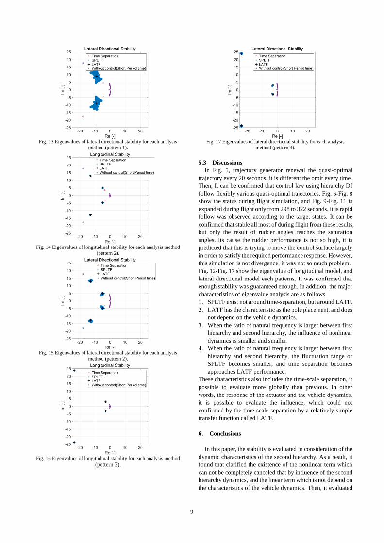
Fig. 14 Eigenvalues of longitudinal stability for each analysis method

(pettern 2).

Fig. 15 Eigenvalues of lateral directional stability for each analysis

method (pettern 2).

Fig. 16 Eigenvalues of longitudinal stability for each analysis method

(pettern 3).

Fig. 17 Eigenvalues of lateral directional stability for each analysis

method (pettern 3).

5.3 Discussions

In Fig. 5, trajectory generator renewal the quasi-optimal

trajectory every 20 seconds, it is different the orbit every time.

Then, It can be confirmed that control law using hierarchy DI

follow flexibly various quasi-optimal trajectories. Fig. 6-Fig. 8

show the status during flight simulation, and Fig. 9-Fig. 11 is

expanded during flight only from 298 to 322 seconds. it is rapid

follow was observed according to the target states. It can be

confirmed that stable all most of during flight from these results,

but only the result of rudder angles reaches the saturation

angles. Its cause the rudder performance is not so high, it is

predicted that this is trying to move the control surface largely

in order to satisfy the required performance response. However,

this simulation is not divergence, it was not so much problem.

Fig. 12-Fig. 17 show the eigenvalue of longitudinal model, and

lateral directional model each patterns. It was confirmed that

enough stability was guaranteed enough. In addition, the major

characteristics of eigenvalue analysis are as follows.

1. SPLTF exist not around time-separation, but around LATF.

2. LATF has the characteristic as the pole placement, and does

not depend on the vehicle dynamics.

3. When the ratio of natural frequency is larger between first

hierarchy and second hierarchy, the influence of nonlinear

dynamics is smaller and smaller.

4. When the ratio of natural frequency is larger between first

hierarchy and second hierarchy, the fluctuation range of

SPLTF becomes smaller, and time separation becomes

approaches LATF performance.

These characteristics also includes the time-scale separation, it

possible to evaluate more globally than previous. In other

words, the response of the actuator and the vehicle dynamics,

it is possible to evaluate the influence, which could not

confirmed by the time-scale separation by a relatively simple

transfer function called LATF.

6. Conclusions

In this paper, the stability is evaluated in consideration of the

dynamic characteristics of the second hierarchy. As a result, it

found that clarified the existence of the nonlinear term which

can not be completely canceled that by influence of the second

hierarchy dynamics, and the linear term which is not depend on

the characteristics of the vehicle dynamics. Then, it evaluated

10

the influence of each terms on around the flight trajectory of

the vehicle. In this model, the control performance using

hierarchy dynamic inversion has been shown to have a affect

of linear terms larger than that of nonlinear terms. In the

numerical simulation, its control performance can be highly

evaluated. Although it is difficult to evaluate to what influence

of the nonlinear terms is small for general aircraft, it think that

the influence is not so significant since the previous research as

well. In the future, in order to realization utilize the hierarchy

DI controller, it is necessary to evaluate the disturbance,

parameter errors, authors are planning to study the influence

each parameters, and evaluation method.

References

1) A. Ishidori,: Nonlinear Control System, Springer-Verlab Berlin, Heidelberg, (1995) , pp. 145-172

2) T. Gang,: Adaptive Control Design and Analysis, John Wiley &

Sons, (2003) , pp. 535-541

3) M. Krstic, L. Kanellakopouios, and P. V. Kokotovic,: Nonlinear and

Adaptive Control Design, Wiley (1995), pp. 64-66

4) P. K. A. Menon, et al.,: Nonlinear Flight Test Trajectory Controller for Aircraft, Journal of Guidance, Control, and Dynamics, 10(1),

(1987), pp. 67-72

5) P. K. A. Menon, et al.,: Nonlinear Missile Autopilot Design Using Time-Scale Separation, Proceeding of the AIAA Guidance,

Navigation, and Control Conference, New Orleans, L.A., August,

AIAA-97-3765, (1997), pp. 1791-1803

6) S. Sunasawa, H. Ohta, Nonlinear Flight Control for a Reentry

Vehicle Using Inverse Dynamics Transformation, Journal of the

Japan Society for Aeronautical and Space Sciences (JSASS),

45(516), (1997), pp. 52-61 (in Japanese)

7) Y. Baba, H. Takano, Flight Control Design Using Nonlinear Inverse

Dynamics, Journal of the Japan Society for Aeronautical and Space

Sciences (JSASS), 47(547), (1999), pp. 122-128 (in Japanese)

9) D. Ito, et al., Reentry Vehicle Flight Controls Design Guidelines:

Dynamic Inversion, Technical Report, NASA/TP-2002-210771

(2002)

10) D. S. Naidu, and J. C. Anthony, Singular Perturbations and Time

Scales in Guidance and Control of Aerospace Systems: A Survey,

Journal of Guicance, Control, and Dynamics, 24(6), (2001), pp.

1057-1078

11) P. Kokotovic, et al, Singular Perturbation methods in control

analysis and design, Society for Industrial and Applied Mathematics,

(1999), pp. 17-40

12) J. Kawaguchi, Y. Miyazawa, T. Ninomiya, Flight Control Law

Design with Hierarchy-Structured Dynamic Inversion Approach,

Proceeding of the AIAA Guidance, Navigation, and Control

Conference, Honolulu, Hawaii, August, (2008), AIAA-2008-6959

13) J. Kawaguchi, T. Ninomiya, H. Suzuki, GUIDANCE AND

CONTROL FOR D-SEND#2, International Congrees of the

Aeronautical Sciences(ICAS), Brisbane, Australia, September,

(2012), 2012-5.3.1

14) T. Ninomiya, H. Suzuki, J. Kawaguchi, Evaluation of Guidance and

Control System of D-SEND#2, IFAC-PapersOnline, 49(17), (2016),

pp. 106-111

15) T. Ninomiya, H. Suzuki, J. Kawaguchi, Controller Design for D-

SEND#2, Journal of the Japan Society for Aeronautical and Space

Sciences (JSASS), 64(3), (2016), pp. 160-170 (in Japanese)

16) A. Abe, Y. Shimada, Flight Control System Using Backstepping

Method for Space Transportation System, Transactions of the

Society for Aeronautical and Space Sciences, Aerospace Technology

Japan, 10-ists28, (2012), Pd_85/Pd_91

17) A. Abe, K. Iwamoto, Y. Shimata, Design of Flight Control System

Based on Adaptive Backstepping Method for a Space Transportation

System, Transactions of the Japan Society for Aeronautical and

Space Sciences, 58(2), (2015), pp. 55-65

16) G. Guna Surendra, et al, Recent Developments of Experimental

Winged Rocket: Autonomous Guidance and Control Demonstration Using Parafoil, Procedia Engineering, 99, (2015),

pp. 156-162

17) K. Itakura, et al., Development and Ground Combustion Test of a Subscale Reusable Winged Rocket, Transactions of the Society for

Aeronautical and Space Sciences, Aerospace Technology Japan,

12-ists29, (2014), To_3_1/To_3_5

18) T.Ohki, et al., Recent Developments of Experimental Winged

Rocket: Autonomous Guidance and Control Demonstration by

Flight Test, Asia-Pacific International Symposium on Aerospace Tchnology, Cairns, Australia, (2015), pp. 408-414

19) K. Yonemoto, T. Fujikawa, et al, Recent Flight Test of

Experimental Winged Rocket and Its Future Plan for Suborbital Technology Demonstration, International Astronautical Congress

(IAC), Guadalajara, Mexico, September, (2016), pp. IAC-16-

D2.6.1

20) H. Yamasaki, K. Yonemoto, et al., Linearization and Response

Analysis of Flight Dynamics Equations Using Multi-Hierarchy

Dynamic Inversion, Japan Joint Automatic Control Conference 59th,

Kitakyushu, Japan, (2016), pp.1054-1059 (in Japanese)

21) S. Miyamoto, T. Narumi, T. Matsumoto, Y. Yonemoto, Real-time

Guidance of Reusable Winged Space Plane Using Genetic

Algorithm Implemented on Field Programmable Gate Array,

Advanced Intelligent Mechatrocics (AIM), KaoHsiung, Taiwan,

(2012), pp. 349-354