Embed Size (px)
Citation preview

UNIVERSIDADE DE LISBOA
FACULDADE DE CIÊNCIAS
DEPARTAMENTO DE FÍSICA
Further Analysis on Cardiovascular Wall
Mechanics with MRI Postprocessing Approaches
Wall shear stress in aorta with coarctation and myocardial systolic
strain in the left ventricle
Maria Manuela Zhu Chen
Mestrado Integrado em Engenharia Biomédica e Biofísica
Perfil em Radiações em Diagnóstico e Terapia
Dissertação orientada por:
Doutora Rita Gouveia Nunes, FCUL
MSc. (Eng.º) João Filipe Fernandes, DHZB
2016

- ii -

- iii -
Abstract
Cardiovascular diseases (CVDs) are the main cause of death worldwide. Irreversible heart complications
are a highly probable outcome when they are left untreated. The congenital CVDs addressed by this
work, coarctation of the aorta (CoA) and aortic valve disease (AvD), have a significant socio-economic
impact. Therefore, providing adequate prognosis and timely treatment should decrease the morbidity
and mortality.
To accomplish this goal, diagnostic medical imaging is a key area to develop. The image acquisition,
processing and clinical parameters outcome need to be assessed with appropriate tools and revised, as
new techniques are constantly being implemented and improved. Two important cardiovascular
parameters that can be evaluated in order to improve diagnosis and intervention in CoA or AvD cases
are the aorta wall shear stress (WSS) and the LV myocardial strain.
To study WSS in aorta with CoA, 16 patients underwent a cardiovascular magnetic resonance (CMR)
exam to obtain phase contrast 4D Flow CMR images. Images were collect before and after aorta
treatment. Post-processing was necessary to obtain WSS values and statistical analysis were performed.
To study LV myocardium strains, namely systolic circumferential strain (ECC) and systolic radial strain
(ERR), 10 datasets were acquired from 8 patients with CoA or AvD before and after intervention with
Cine and Tagging sequences of CMR images. The post-processing of the images was done using two
techniques (Tagging HARP and Feature Tracking) that were applied independently to measure those
strains. The validation of one technique against the other was performed through Bland-Altman method.
Lastly, strain values estimated before and after intervention were statistically compared.
The WSS study showed that in general WSS values are increased after CoA treatment. Although,
statistically, only some values revealed a significant increase (p < 0.05). The myocardial strain study
demonstrated a good agreement between the two strain measurement techniques and showed no
statistically difference (p > 0.05) between strain values estimated before and after treatment for both ECC
and ERR.
The evaluation of cardiovascular parameters is important to forecast the evolution of a disease by, for
example, predicting the LV or heart remodelling after intervention. Thus, the possibility to identify
patients at risk of future heart complications could be timely and properly provided.
Keywords: Cardiovascular Magnetic Resonance, Wall Shear Stress, Myocardium Strain, CMR Tagging,
Feature Tracking.

- iv -

- v -
Resumo
De acordo com os dados da Organização Mundial da Saúde de 2016, as doenças cardiovasculares são a
principal causa de morte a nível mundial. Quando não tratadas em tempo adequado ou simplesmente
não tratadas, podem resultar, com uma grande probabilidade, em insuficiências cardíacas ou outras
complicações irreversíveis.
As duas doenças cardiovasculares congénitas estudadas neste trabalho são a coarctação aórtica (CoA),
caracterizada por uma estenose na aorta, habitualmente na porção descendente da artéria, e a doença da
válvula aórtica (AvD, sigla em inglês). Como mais de 50 000 intervenções são realizadas por ano na
União Europeia, estas doenças têm um impacto socioeconómico significativo. Assim sendo,
prognósticos adequados e tratamentos no período adequado são factores importantes que podem levar
ao decréscimo no número das intervenções bem como reduzir a morbilidade e a mortalidade.
Para tal, a área de imagiologia médica de diagnóstico é fundamental. A aquisição de imagens médicas,
o posterior processamento e os parâmetros clínicos resultantes têm que ser avaliados com recurso a
programas adequados, e os métodos de análise constantemente melhorados. De modo a permitir uma
melhor intervenção ou reparação da coarctação aórtica e da doença da válvula aórtica, dois importantes
parâmetros biomecânicos cardíacos são estudados neste trabalho. São eles a tensão de cisalhamento na
parede aórtica (WSS, em inglês), que permite avaliar as condições do fluxo sanguíneo e o estado da
parede dos vasos sanguíneos, e a deformação do miocárdio a nível do ventrículo esquerdo que, por sua
vez, permite avaliar a contractilidade do ventrículo.
No estudo da WSS nas aortas com estenose, 16 pacientes (idade média de 19 ± 11 anos, faixa etária 7
a 46 anos, 13 masculinos e 3 femininos) submeteram-se à ressonância magnética cardiovascular de
contraste de fase em tempo real (4D PC MRI, em inglês) de modo a recolher imagens a nível da aorta e
os respectivos padrões de velocidade da corrente sanguínea. Essa recolha foi feita duas vezes, uma antes
do tratamento da estenose e outra após o tratamento. As imagens recolhidas foram posteriormente
processadas em programas específicos: numa primeira fase foi necessário segmentar a aorta, seguida de
obtenção de valores de velocidade ao longo da aorta e, posteriormente, o cálculo dos valores da tensão
de cisalhamento da parede aórtica. Dado que o WSS é um parâmetro que varia ao longo de um ciclo
cardíaco, é de notar que os valores obtidos correspondem a WSS’s máximos, mínimos e médios nas três
porções que constituem a aorta (ascendente, transversal e descendente torácica). Por último, testes
estatísticos (teste t para amostras com distribuição normal, caso contrário, teste de Wilcoxon) foram
aplicados de modo a comparar os valores de WSS antes e depois do tratamento.
No estudo da deformação do miocárdio a nível do ventrículo esquerdo, nomeadamente a deformação
circunferencial sistólica (ECC) e a deformação radial sistólica (ERR), 8 pacientes (idade média 34 ± 23
anos, faixa etária 10 a 61 anos, 6 masculinos, 2 femininos) com CoA ou AvD foram inseridos no estudo.

- vi -
Ao todo foram recolhidos nestes pacientes 10 conjuntos de dados (cada conjunto incluí valores de ECC
e de ERR), usando as sequências cine e tagging das suas imagens de CMR, antes e depois do tratamento.
A recolha foi realizada através de duas técnicas aplicadas independentemente, ou seja, 10 conjuntos de
dados para cada uma das técnicas e obtidos em condições similares. As técnicas são CMR Tagging
HARP (aplicada às as sequências tagging) e CMR Feature Tracking (aplicadas às sequências cine),
sendo a primeira de referência. HARP é considerado como sendo o método mais rápido no
processamento de imagens tagging mas a Feature Tracking (FT) é mais rápida e simples no que toca à
medição dos valores de deformação por ser aplicada directamente a sequências cine. A validação da
técnica FT com a de referência, baseada nos valores de deformação (ECC e ERR), foi analisada através
do método de Bland-Altman. Adicionalmente, os valores de deformação antes e após o tratamento,
obtidos pela técnica FT, foram estatísticamente comparados, usando o teste t ou o teste de Wilcoxon
consoante a existência ou não de normalidade nas amostras.
O trabalho do WSS demonstrou que em geral os valores de WSS aumentam após o tratamento da
estenose aórtica, embora, estatisticamente, apenas alguns valores de WSS em algumas porções da aorta
(WSS médio na porção ascendente, todos os WSS’s na porção transversal e valores de WSS min. na
porção descendente) aumentaram de um modo significativo (p-values entre 0.009 e 0.038 para um nível
de significância de 5%). Esta parte do trabalho serviu também para validar o programa utlizado na
obtenção dos WSS’s contra valores publicados em estudos anteriores, dado que corresponde à primeira
versão.
A avaliação da deformação miocárdica demonstrou que existe uma boa concordância entre as duas
técnicas de medição baseando nos resultados obtidos pelo método de Bland-Altman, principalmente
para ECC (bias ≈ – 2.02 % e limites de concordância de – 10.5 a 6.4 %). Verificou-se que resultados
semelhantes foram obtidos em vários estudos anteriores. Observou-se também que as alterações na
deformação miocárdica com o tratamento não foram estatisticamente significativas para ambos os tipos
de deformação estudados, a ECC e a ERR (p-values > 0.05 ao nível de significância de 5%).
Em conclusão, os resultados obtidos com este trabalho poderão fornecer informações importantes
relativamente à evolução das doenças aqui estudadas com o tratamento. A contractilidade do ventrículo
esquerdo é alterada quando o coração é sujeito a intervenções, resultando na alteração da forma do
ventrículo (remodelling) a longo prazo. Assim sendo, a análise da deformação do tecido miocárdico
torna-se essencial para perceber como essa alteração é verificada. Adicionalmente, a validação da
Feature Tracking contra a Tagging permitiu reforçar conclusões de estudos anteriores: a FT é um
método válido que pode subtituir a Tagging, principalmente, na análise da deformação circunferencial
do miocárdio.
Palavras-Chave: Ressonância Magnética Cardiovascular, Tensão de Cisalhamento da Parede Aórtica,
Deformação do Miocárdio, CMR Tagging, Feature Tracking.

- vii -
Contents
ABSTRACT iii
RESUMO v
CONTENTS vii
ACKNOWLEDGMENTS ix
LIST OF FIGURES xi
LIST OF TABLES xiii
LIST OF ABBREVIATIONS AND ACRONYMS xiv
MOTIVATION/ TOPIC OVERVIEW xv
THESIS OUTLINE xvii
I. CONCEPTS AND THEORETICAL BACKGROUND 1
I.1. Cardiovascular structures under focus 1
I.2. Congenital heart diseases under focus 3
I.3. Basic Principles of MRI 5
I.4. Cardiac Magnetic Resonance 9
I.5. Techniques of CMR 11
I.6. Cardiovascular parameters under focus 18
II. OBJECTIVES 25
II.1. Wall Shear Stress 25
II.2. CMR-Tagging vs CMR-FT 25
III. MATERIAL 27
III.1. CMR scanner and Image Acquisition Protocol 27
III.2. Post processing tools 28
IV. WALL SHEAR STRESS IN AORTA WITH COARCTATION STUDY 35
IV.1. Methodology 35
IV.2. Results 37
IV.3. Discussion 41

- viii -
V. MYOCARDIAL SYSTOLIC STRAIN IN THE LEFT VENTRICLE 43
V.1. Methodology 43
V.2. Results 47
V.3. Discussion 50
VI. CONCLUSION 53
REFERENCES 55

- ix -
Acknowledgments
Firstly, I would like to express my sincere gratitude to my advisors Prof. Rita Nunes and Eng. João
Fernandes for the continuous support of my work, for their knowledge and patience in reviewing the
thesis several times. Their guidance was essential during all the time necessary for this thesis
development. I could not have imagined having better advisors for my master dissertation. An extra
special thanks to João for the days in Berlin!
My sincere thanks also goes to Dr. Titus Kühne who provided me the opportunity to join the Deustches
Herzzentrum Berlin (DHZB) MRI team as intern. I would also like to thank the rest team members that
kindly accompanied me during the internship, providing me with good suggestions and made my days
at the work brighter: Eng. Tiago Silva, Dr. Marcus Kelm, Dr. Sarah Nordmeyer and Alireza Khasheei.
Many thanks to the Professors of the Institute of Biophysics and Biomedical Engineering for enriching
our academic experience and being always supportive.
I want to thank also one of my closest friends and colleague Vera Colaço for sharing with me
unforgettable adventures during the internship period. In addition, I would like to thank the friends that
I have met in Berlin for the meaningful and fulfilling moments that we built together back then.
Last but not least, I must express my very profound gratitude to my lovely family: my parents, my
brother, my sisters and my little nephews for providing me with unfailing support and continuous
encouragement throughout all these years of study and through the elaboration of this thesis. All these
accomplishments would not have been possible without them and I hope I can pay them back somehow
in a near future. Thank you!

- x -

- xi -
List of Figures
Figure I.1. Representation of the human heart structure and blood flow pathways. Adapted from [11]. ................................... 1
Figure I.2. The figure shows a segmented aorta (blue), left ventricle without myocardium (green) and left atrium (yellow) in a
coronal perspective and based on MRI images obtained from the patients with coarctation. ..................................................... 2
Figure I.3. Same segmentation than the one in the figure above but in this case the left ventricle is sheltered by the myocardium
(pink). ......................................................................................................................................................................................... 2
Figure I.4. CMR lateral view in an 11 years old paediatric patient with aortic coarctation (arrow). Image from the study of wall
shear stress in CoA patients. ....................................................................................................................................................... 3
Figure I.5. Precessional path of magnetic moment of hydrogen nuclei, depending on their energy, it can be a spin up nuclei
(parallel to B0) or a spin down (anti-parallel to B0) nuclei. Adapted from [22]. ......................................................................... 6
Figure I.6. Standard 2D CINE PC MRI gated to ECG, with one-directional (Vz) blood flow velocity encoding. Reference and
velocity sensitive scan (bipolar encoding gradient added) are acquired in direct succession. By subtracting the reference and
the flow sensitive datasets, phase difference images can be obtained, which contain quantitative blood flow velocities. Flow
velocities in the predominant blood flow direction appear bright (AAo and PA) while blood flow velocities in the opposite
direction appear dark (DAo). Due to time limitations, a single heartbeat is not sufficient to acquire all PC-MR data, thus data
is collected over several cardiac cycles. The measurement is synchronized with the cardiac cycle using an ECG-gated k-space
segmented data acquisition. AAo – ascending aorta PA – pulmonary artery DAo – descending aorta. Adapted from [29]. ... 12
Figure I.7. Cartesian 4D flow MRI at the thoracic aorta region. For each time frame, four 3D raw datasets are collected to
measure three-directional blood flow velocities (Vx, Vy, Vz): a reference scan and three velocity-encoded acquisitions. Instead
of one velocity sensitive scan, in 4D Flow PC-MR three directional flow velocity sensitive scans are acquired. Navigator gating
of the diaphragm motion can be used for free-breathing image acquisition. Adapted from [29]. ............................................ 13
Figure I.8. MRI SPAMM short axis images of left ventricle captured during a cardiac cycle. Adapted from [38]. ................. 15
Figure I.9. HARP – The frequency domain of a tagged image, composed by harmonic magnitude and harmonic phase, is
analysed. Adapted from the handbook provided with the Diagnosoft software. ...................................................................... 16
Figure I.10. HARP Technique – spatial phase-change of the tagging lines determines the deformation measurement and motion
tracking (left); the different strains magnitude measured are represented through a color map (right). Adapted from the
handbook provided with the Diagnosoft software. ................................................................................................................... 16
Figure I.11. Left – manual endocardial trace in a short axis plane. Right – tracked endocardial trace in a short axis plane.
Adapted from [43]. ................................................................................................................................................................... 17
Figure I.12. WSS among other conditions such as blood pressure, cyclic strain and chemical messengers (endocrine, autocrine,
paracrine) are some of the biomechanical conditions that interfere with the endothelial cells of the blood vessels. As represented
in the figure, WSS is a tangential force over the endothelial surface; in ideal flow conditions, in laminar flow, WWS presents
the same direction than the blood flow. Adapted from [45]. .................................................................................................... 18
Figure I.13. Representation of blood flow velocity direction and shear stress direction. Adapted from [45]. .......................... 19
Figure I.14. Spatial distribution of WSS along an aorta with coarctation from a 10 years old patient. Results obtained through
CMR 4D Flow technique. Image from the study of WSS in CoA patients. ............................................................................. 20
Figure I.15. The Resulting Image is a short axis view obtained by placing the imaging plane perpendicular to the septum and
parallel to the mitral valve (as represented in the Planning Image –a 4-chamber view of the heart). ....................................... 22

- xii -
Figure I.16. 3D-RCL coordinate system used for strain calculation. Adapted from [35]. ........................................................ 22
Figure III.1. ZIBAmira software. CMR images from an 11 years old patient before treatment represented in transversal, sagittal
and coronal planes (clockwise from upper left to bottom left). The image on the bottom right corner right down corner, already
shown in chapter I.1., corresponds to the multi label segmentation of the left heart: aorta (blue), left ventricle (right), and left
atrium (yellow, not fully seen in this perspective). ................................................................................................................... 29
Figure III.2. ZIBAmira software. Same set of images than in Figure III.1, but now the image at the bottom right corner, already
shown in chapter I.1., corresponds to the multi label segmentation of the left heart: aorta (blue), left atrium (yellow, now in
another perspective) and myocardium (pink, with the LV hidden inside). ............................................................................... 29
Figure III.3: MevisFlow platform. In order to obtain WSS, blood velocity data inside the aorta needs to be calculated. To do
so, the aorta segmentation previously obtained is uploaded together with the magnitude and the three directional field CMR
images to the MevisFlow software. .......................................................................................................................................... 30
Figure III.4. WSS Explorer platform. Results from the MevisFlow software are uploaded into the WSS Explorer platform. The
WSS values are calculated in the regions where planes are placed (in this image we have a total of 18 planes along the aorta).
................................................................................................................................................................................................. 31
Figure III.5. CAIPI platform. The user can select which time step of the whole CMR sequence and which level of the LV the
user wants to obtain measurements from. In the present work, the aim was to calculate myocardial systolic strain at the mid
level of the LV. ........................................................................................................................................................................ 32
Figure III.6. FT software. Short axis LV CMR images were uploaded to the platform. Myocardium at the mid-level of the LV
was manually selected at the first instance and then propagated automatically through the remaining time steps that form the
cardiac cycle. Myocardial strain results are then calculated. .................................................................................................... 33
Figure IV.1. Left: CMR image, from an 11 years old male patient before treatment. Right: The respective aorta WSS
measurement in different regions (represented in the aorta by the several planes) before treatment, values estimated using the
MEVIS WSS Explorer. The stenosis region is indicated by a red plane. ................................................................................. 37
Figure IV.2. Left: The respective CMR image, from the same 11 years old male patient, after treatment; it is possible to see the
stent (indicated in the image by the red arrow) put inside the aorta as a treatment for the stenosis. Right: The respective aorta
WSS measurement in different regions (represented in the aorta by several planes) after treatment, using the MEVIS WSS
Explorer. ................................................................................................................................................................................... 37
Figure IV.3. Aorta WSS measurement for 6 of the 16 patients; shape, size and length differ from person to person. ............. 38
Figure IV.4. Min WSS values in ascending, transversal and descending part of the aorta in pre and post treatment conditions.
................................................................................................................................................................................................. 39
Figure IV.5. Max WSS values in ascending, transversal and descending part of the aorta in pre and post treatment conditions.
................................................................................................................................................................................................. 39
Figure IV.6. Mean WSS values in ascending, transversal and descending part of the aorta in pre and post treatment conditions.
................................................................................................................................................................................................. 40
Figure IV.7. OSI values in ascending, transversal and descending part of aorta in pre and post treatment conditions. ........... 40
Figure V.1. Diagnosoft VIRTUE software using a CMR tagging (with grid) image. A mesh is created around the myocardium
after manually placing points first (yellow for endocardium and green for epicardium; the orange mid-wall line and the
remaining lines are automatically created after the previous one). The blue arrow indicates the separation between LV and RV
by the septum in the anterior region. ........................................................................................................................................ 44

- xiii -
Figure V.2. Representation of the short axis slice at mid-ventricle level. ............................................................................... 44
Figure V.3. FT software. Below: CMR image representing the left side of the heart at the mid LV level in a short axis plane.
LV endocardium is delimited in blue and epicardium in yellow, those are the myocardium contours used to initiate the automatic
myocardial strain FT throughout the cardiac cycle. Right: 3D AHA model of the LV constructed after placing the orientation
points; the plane represented below is the one crossing the 3D LV model at mid-level. .......................................................... 45
Figure V.4. Left: Histogram and Gaussian plot of the difference between CMR Tagging and CMR FT derived peak systolic
circumferential strain. Right: Histogram and Gaussian plot of the difference between CMR Tagging and CMR FT derived peak
systolic radial strain. ................................................................................................................................................................. 46
Figure V.5. Bland-Altman plot comparing mean peak systolic circumferential strain (ECC) for tagging and feature tracking
techniques. Mean ECC difference (bias) of – 2 % and limits of agreement [ –10.5; 6.4] %. ..................................................... 48
Figure V.6. Bland-Altman plot comparing mean peak systolic radial strain (ERR) for tagging and feature tracking techniques.
Mean ERR difference (bias) of 13.06 % and limits of agreement [– 8.5; 34.6] %. .................................................................... 48
Figure V.7. Comparison of CMR Tagging versus CMR FT derived peak systolic ECC in patients with CoA or AvD. ........... 49
Figure V.8. Comparison of CMR tagging versus CMR FT derived peak systolic ERR in patients with CoA or AvD. ............. 49
Figure V.9. Comparison of CMR FT derived peak systolic ECC before and after treatment in patients with CoA................... 49
Figure V.10. Comparison of CMR FT derived peak systolic ERR before and after treatment in patients with CoA. ................ 49
List of Tables
Table 1. Patient’s characteristics from WSS study. Treatments: I – Balloon Angioplasty; II – Stent implant; III – Pre-stent
dilation; IV – Medical treatment. ............................................................................................................................................. 35
Table 2. WSS study results. Values of WSS (in Pa) measured in the three sections of the aorta before (pre) and after (post)
CoA correction and the respective p-values. Significant results are indicated by (*). .............................................................. 38
Table 3. Patient’s characteristics from the validation of FT against tagging study, based on the LV myocardium strain. All the
8 patients recorded tagging and FT images; column “CMR Images” describes in which stage (pre or post treatment) the
images were collected and then used in the study. ................................................................................................................... 43
Table 4. Patient’s characteristics from the validation of FT against tagging study and the respective values of ECC and ERR
from both of the techniques. ..................................................................................................................................................... 47

- xiv -
List of Abbreviations and Acronyms
AAo Ascending Aorta
TAo Transversal Aorta
DAo Descending Aorta
AvD Aortic Valve Diseases
CMR Cardiovascular Magnetic Resonance
CoA Aortic Coarctation
ECC Systolic Circumferential Strain
ERR Systolic Radial Strain
FT Feature Tracking
LV Left Ventricle
MRI Magnetic Resonance Imaging
Venc Velocity Encoding
WSS Wall Shear Stress
2D Two Dimensional
3D Three Dimensional
4D Four Dimensional

- xv -
Motivation/ Topic Overview
Cardiovascular diseases (CVDs) are the main cause of death worldwide [1]. Irreversible heart
complications are a highly probable outcome when CVDs are left untreated. The two diseases addressed
by this work, coarctation (CoA) and aortic valve disease (AvD), have a significant socio-economic
impact, as they motivate more than 50 000 interventions per year within the EU [2]. Providing adequate
prognosis and timely treatment is undoubtedly a necessary approach to improve diagnosis and
interventions.
To accomplish this goal, diagnostic medical imaging is a key area to develop. The image acquisition,
processing and clinical outcome need to be assessed with appropriate tools and revised, as new
techniques are constantly being implemented and improved. Two important cardiovascular mechanical
parameters that can be evaluated to obtain a more complete understanding of the aorta and left ventricle
(LV) coupling in CoA or AvD cases, are the aorta wall shear stress (WSS) and the LV myocardial
contractility, which is analysed through strain measurements.
Wall shear stress (WSS) is an important parameter for testing blood flow and vessel inner conditions.
Some previous works have already studied this parameter in patients with AvD and in some portions of
the aorta in patients with CoA [3]–[6]. With this work, the goal was to collaboratively develop and test
a new software that calculates regional and global WSS along the main vessels; in this case, along the
aorta artery (ascending aorta, aortic arch and thoracic descending) before and after coarctation treatment.
CMR tagging has been considered a gold standard technique for myocardial deformation measurements.
However, it is a slow and complex process that requires the acquisition of additional MRI images.
Feature Tracking (FT) method has proved to be a suitable replacement for tagging. It has already been
successfully tested against tagging in several cardiovascular diseases in order to evaluate some
parameters such as circumferential strains [7]–[10]. The present work aimed to analyse the impact of
aortic CoA and AvD interventions on myocardial remodelling by analysing LV deformation and to test
the accuracy of the new FT software (Fraunhofer MEVIS, Bremen, Germany) against tagging in a set
of patients.

- xvi -

- xvii -
Thesis Outline
The dissertation is composed by 6 main chapters (I to VI).
In chapter I, concepts and definitions that form the basis of this work are introduced. At first, anatomy
and physiology of relevant cardiovascular structures (aorta, left ventricle and aortic valve) are briefly
exposed, followed by the description of the congenital heart diseases that affect those structures (CoA
and AvD). CoA is explained in more detail as most of the intervenient patients present this congenital
condition. Subsequently, a summary of the basic principles behind MRI is provided before introducing
CMR and its techniques, with special focus on the 4D Flow CMR, CMR Tagging and FT. The
cardiovascular parameters (WSS and myocardial strains) are the topic of the last section of this chapter.
In chapter II, the two main objectives of this dissertation are presented: the first one, regarding the
evaluation of the WSS parameter in patients with CoA, and the second one, the validation of the FT
against CMR Tagging in patients with CoA or AvD and evaluation of the myocardial strain parameters
in these patients.
In chapter III, the material used to develop this work is presented. Firstly, a description of the CMR
scanner and image acquisition protocol are provided. Then, brief introductions of the post-processing
tools used to analyse the CMR images and to collect the data are presented. The tools used and the steps
followed with some programs are described in more detail in chapters IV and V.
In chapter IV, the study “WSS in aorta with CoA” is presented, with subsections methodology, results
and discussion.
In chapter V, the study “Myocardial systolic strain in the LV” is presented comprising the subsections
methodology, results and discussion.
Finally, in the chapter VI, the overall conclusions are presented regarding both studies and expected
future perspectives in the CMR imaging field and the respective medical parameters that can be obtained
by the studied techniques.

- xviii -

- 1 -
I. Concepts and Theoretical Background
Relevant concepts and theoretical background that form the basis for the development of this work are
introduced in this chapter.
I.1. Cardiovascular structures under focus
I.1.1. Aorta
Aorta is the main blood vessel carrying oxygen-rich blood from the heart to all systemic arteries. It is
divided in 3 principal regions: ascending aorta, which rises from the left atrium and corresponds to the
proximal and ascending segment of the aorta (the coronary arteries are only branches of this segment);
aortic arch, which has an inverted U form and it is the origin of 3 major arteries (brachiocephalic trunk,
left common carotid artery and left subclavian artery); and descending aorta, the longest and more distal
section of the aorta that is divided in two portions (thoracic aorta, above the diaphragm, and abdominal
aorta, below it) [11]. The position of the aorta in the heart can be seen in Figure I.1 and a segmentation
of the aorta is represented in Figures I.2 and I.3.
Figure I.1. Representation of the
human heart structure and blood
flow pathways. Adapted from
[11].

- 2 -
I.1.2. Left Ventricle
The LV has heterogeneous material properties, its geometry is complex and, due to its functions, it
undergoes large deformations. Comparing to the right ventricle and to the two atria, the LV has the
thickest wall. In adults, the lateral wall measures almost 1 cm in thickness in a normal left ventricle [12].
As it contracts, the oxygen-rich blood is pumped out through the aortic valve into the aorta and onward
to the rest of the body. Several conditions can affect its proper working. The heart wall, as the LV wall,
is composed of three layers: a thin epicardium covering its external surface, a thick muscular
myocardium in the middle (a segmentation of the myocardium is represented in Figure I.3.), and a thin
endocardium lining the interior of the chambers. LV is separated from the right ventricle by the
interventricular septum that bulges toward the right ventricle. In the short axis view plane, LV has a
circumferential format [13].
I.1.3. Aortic Valve
Between the LV and the aorta, we have the aortic valve (Figure I.1); it is responsible for a normal and
controlled blood flow from the left atrium to the whole arterial system from the aorta. In normal
conditions, three leaflets compose the aortic valve, although congenitally affected patients may have
only two leaflets [11].
Figure I.2. The figure shows a segmented
aorta (blue), left ventricle without
myocardium (green) and left atrium
(yellow) in a coronal perspective and
based on MRI images obtained from the
patients with coarctation.
Figure I.3. Same segmentation than
the one in the figure above but in this
case the left ventricle is sheltered by
the myocardium (pink).

- 3 -
I.2. Congenital heart diseases under focus
Congenital heart diseases (or defects) are problems with the structure of the heart that are present at birth
and affect the heart function by changing the normal blood flow through it. In some cases, these
problems can be detected during pregnancy. Due to their localization, they cause more deaths in the first
year of life compared to any other birth defects. There are several forms of congenital heart diseases,
ranging from simple defects with no symptoms at all or no symptoms until adulthood, to the complex
ones with severe and life threatening symptoms. Usually, they are divided into two main groups:
cyanotic, due to the blue skin colour caused by a lack of oxygen, and non-cyanotic.
I.2.1. Coarctation
Coarctation of the aorta (CoA) is a narrowing of part of the proximal descending aorta (Figure I.4).
When the CoA segment is located within less than 10 mm from the origin of the left subclavian artery
it is defined as proximal CoA and when it is located further than 10 mm, it is defined as distal CoA [14].
CoA accounts for 5 to 7% of all congenital heart disease [15], being the sixth most common form of
heart congenital disease [16] and with an estimated incidence of around 3 cases per 10000 live births
[15].
CoA can be present in different forms across all age ranges and under varying clinical symptoms
associated with other heart problems or in an isolated way. In some cases, CoA can be asymptomatic
during earlier stages of life or during the whole lifetime.
Detection and evaluation of CoA can be made by different techniques. Transthoracic echocardiography
is the standard initial test of choice for CoA detection in both children and adults; in neonates and infants,
Figure I.4. CMR lateral view in an
11 years old paediatric patient with
aortic coarctation (arrow). Image
from the study of wall shear stress
in CoA patients.

- 4 -
it can be used to measure the severity of the CoA and detect other cardiac defects. In cases where the
echocardiographic window is suboptimal for CoA detection or evaluation, CMR or Computed
Tomography (CT) techniques are used. Anatomical images of CoA provided by CMR or CT scan can
be used to create 3D images for clinical or research purposes. Collateral vessel flow can be assessed by
CMR as well. Regarding chest X-ray, it is more specific in older patients. Cardiac catheterization is
mostly used nowadays for therapeutic intervention, whereas in the past it was frequently used for
diagnosis.[15]
The first surgical repair of CoA was performed in 1944 [15], since then, other treatment techniques have
also been developed and refined. Balloon angioplasty was first described by Lock et al in 1982 [17]. In
children, it is rather more adequate for recurrent CoA than for native coarctation, as in the latter case,
the probability of aneurysm formation seems to be higher [15]. Endovascular stent placement was
introduced in 1991 [18], complementing the trans-catheter treatment. Endovascular stents are placed in
the vessels through balloon catheters. Besides supporting the vessel wall, stents also decrease aortic wall
injuries and restenosis verified in balloon angioplasty alone [19]. Still, due to the risk of aneurysm after
balloon angioplasty or the need for re-dilatation with stent placement, surgical repair is preferable for
the infant and young children with native CoA [15].
To assess the degree of a CoA, the blood pressure gradient across the narrowing of the aorta is measured.
The main indication for intervention is this pressure gradient being higher than 20 mmHg. [20]
Currently, both surgical and endovascular treatments (stent and balloon angioplasty) are used for CoA
in order to relieve the obstruction. However, patients are still at risk of facing recurrent CoA, aneurysm
formation after intervention, persistent hypertension, and changes in any associated cardiac defects. The
decision for the most reasonable treatment intervention depends always on the complexity of the CoA,
age at presentation, and whether or not it is a native or recurrent narrowing. [15]
I.2.2. Aortic Valve Disease
The AvD includes aortic valve stenosis and/ or regurgitation. In normal conditions, the aortic valve
ensures a unidirectional blood flow out of the heart. In aortic valve stenosis, the valve does not open
fully due to its narrowed form and the restricted motion of its leaflets, therefore a decrease in the blood
flow from the heart is verified. In aortic regurgitation, one or more of the leaflets are stretched out, torn
or stiffened, affecting the closure of the valve in every heartbeat and allowing backward blood flow.
As the blood flow into and out of the heart is affected, the LV needs to work more intensively in order
to pump the blood out through the valve. This added workload can remodel the LV’s shape. Imaging
modalities such as CMR have been improved and increasingly utilized in the management of AvD.
CMR can depict the morphology and severity of the aortic valve and assess its consequences on LV.
[21]

- 5 -
I.3. Basic Principles of MRI
In order to have a better understanding of the imaging modalities used in this work, it is important, firstly,
to discuss briefly the basic principles of MRI.
I.3.1. MR active nuclei
The MR active nuclei are characterised by their ability to acquire a magnetic moment (due to their
spinning motion and the possession of a net of charge). The acquired magnetic field enables them to
align with an external applied magnetic field (B0). The process is possible if the mass number is odd.
Spin or spin angular momentum is the quantum property that describes the rotational spinning
movement of the nuclei. The abundancy of hydrogen (H1) in the human body and its unique proton
makes it the most important MR active nuclei in MRI. [22]
I.3.2. Alignment
Magnetic moments of H1 nuclei orient in a random way when no magnetic field is applied. However, in
the presence of a strong static B0, most of the H1 nuclei align with it in a parallel way (same direction
than B0, low-energy status) and some in anti-parallel way (opposite direction than B0, high-energy
status). The direction of the alignment is determined by the strength of B0 and together with the thermal
energy level of the nuclei, a result of body temperature. As the strength of B0 increases, the energy
difference between the two states increases. Nuclei with low thermal energy do not have sufficient
energy to oppose the B0 in the anti-parallel direction, only nuclei with high thermal energy can do so.
Thus, magnetic moments of nuclei that aligns parallel to B0 cancel out the smaller amount of those
aligned in an anti-parallel way and the small excess in the parallel direction produces a net magnetic
moment. [22]
H1 nuclei are used in clinical MRI because its net magnetic moment originates a significant net magnetic
vector (NMV). The interaction of the NMV with B0 is the basis of MRI. The magnitude of NMV is
larger at high B0 field strengths as fewer nuclei exist in the high-energy status. [22]
I.3.3. Precession and the Larmor equation
Every H1 nucleus that contributes to the NMV spins on its own axis and under the influence of B0, the
NMV vector oscillates in a circular path around B0, Figure I.5. Precession frequency is the frequency
(0) at which the NMV wobbles around B0 and it is described by the Larmor equation:
0 = B0 (MHz) Equation I.1

- 6 -
Where γ is the gyro-magnetic ratio, a constant that expresses the relationship between the angular
momentum and the magnetic moment of each MR active nucleus; it can also be interpreted as the
precessional frequency of a specific MR active nucleus at 1.0 T, its unit is MHz/T. hydrogen = 42.57 MHz/
T. [22]
I.3.4. Resonance
When a nucleus is exposed to an external source of perturbation with a similar oscillation to its own
natural frequency, it absorbs energy and resonates if the energy is delivered at the same frequency than
the Larmor frequency (0). In MRI, the radio frequency (RF) band corresponds to the energy at the
precessional frequency of H1 placed at any magnetic field strength. Resonance occurs when RF pulses
of energy equal to the Larmor frequency of H1 NMV are applied. As the Larmor frequency of each type
of MR active nuclei is different, only H1 nuclei resonate. [22]
The global result of resonance are flipping of the NMV (measured in terms of flip angle and controlled
by the RF pulse) towards transverse plane at the Larmor frequency and phasing of the magnetic moments
(i.e. moving together in the same position) on the precessional path.
I.3.5. The MR signal
The NMV precession in the transverse plane is a moving magnetic field that creates magnetic
fluctuations inside a receiver coil. According to Faraday’s induction law, if a receiver coil or any
conductive loop is in interaction with a moving magnetic field, a voltage is induced in the coil. Thus, an
electrical signal is produced (the induced voltage), corresponding to the MR signal. It has the same
frequency as the Larmor frequency and the amount of magnetization existing in the transverse plane
determines the magnitude of the signal.
Figure I.5. Precessional path of magnetic moment of hydrogen nuclei, depending on their energy, it can
be a spin up nuclei (parallel to B0) or a spin down (anti-parallel to B0) nuclei. Adapted from [22].

- 7 -
Gradient coils located inside the main magnet generate magnetic field gradients. They are used to alter
the main static magnetic field by increasing or decreasing the field strength. The variation in the field
strength allows localization of slice planes as well as phase encoding and frequency encoding. Thus,
spatial encoding of the MR signal involves the use of magnetic field gradients. [22]
I.3.6. K-space
The generated MR signal data has to be collected before producing the respective MR image. This raw
MRI data is, therefore, stored in matrix form, called k-space. K-space is a spatial frequency domain,
where the relative contribution of the different spatial frequencies in the patient image are registered
[22]. It is commonly defined by a rectangular grid with two main axes that are perpendicular to each
other. The vertical axis is related to the signal frequency encoding and the horizontal one to the signal
phase encoding. Inverse Fourier Transform is used to generate the MR image. Each pixel in the image
results from all the individual points in k-space. Conversely, each point in k-space contains spatial
frequencies and phase information regarding every pixel in the image.
In the 4D Flow Phase Contrast technique, k-space is used to collect data from multiple cardiac cycles in
order to produce a complete 4D flow data. The complete data is composed only by fractions of each
cardiac cycle. The technique is known by “k-space segmentation”. [23]
I.3.7. The free induction decay signal (FID)
When the RF pulse is switched off, the NMV starts to realign with B0. The realignment is done by the
process of relaxation; there is a gradual recovery (T1 recovery) of magnetisation in the longitudinal axis
as the NMV returns the amount of RF energy absorbed. Simultaneously but independently, occurs a
gradual decay (T2 decay) of magnetisation in the transverse plane as the magnetic moments diphase.
When T2 decay occurs, the inducted voltage, i.e., the MR signal is consequently reduced. The signal
measured during this recovery period is named as free induction decay (FID). [22]
I.3.8. Pulse timing parameters
A simplified pulse sequence is a combination of RF pulses, signals and intervening periods of recovery;
Repetition time (TR), echo time (TE) are the main components of a pulse sequence. TR is the time from
the application of one RF pulse to the application of the next RF pulse, expressed in milliseconds (ms);
it determines the amount of T1 relaxation that has occurred, i.e., the amount of relaxation that is allowed
to occur between the end of one RF pulse and the application of the next. TE is the time from the
application of the RF pulse to the peak of the signal induced in the coil, expressed in ms; it controls the

- 8 -
amount of T2 decay that has occurred, i.e., how much decay of transverse magnetization is allowed to
occur before the signal is read. The contrast in MRI images is produced by the application of RF pulses
at certain TRs and by the receiving of signals at pre-defined TEs. [22]
I.3.9. Pulse sequences
Pulse sequences are designed for different purposes. Different pulse sequences are a result of different
magnitude and timing of radiofrequency pulses emitted by the MR scanner, which is programmed in
and controlled by software programs [12]. Pulses can be originated by application of magnetic field
gradients.
Spin Echo sequences use a 90° excitation pulse to flip the NMV into the transverse plane followed by
one or more 180° re-phasing pulses to create one or more spin echoes. According to the different images
that one wants to obtain, TE and TR adjustments are made in order to generate one or more echoes.
Gradient Echo sequences use a variable RF excitation pulse that flips the angle of the NMV in order to
reduce TR without producing saturation; TR is directly related to the scan time. Gradient-echo sequences
are used to quantify blood velocity and flow with encoding of velocity in the signal phase [24]. Finally,
in Steady State Free Precession (SSFP), a steady state condition, TR is shorter than T1 and T2 times of
the tissues; consequently, longitudinal magnetization coexists with transverse magnetization because
the pulse sequence is repeated again before the full decay of the transverse magnetization; SSFP is
considered a fast sequence [22], [25].

- 9 -
I.4. Cardiac Magnetic Resonance
CMR or cardiac MRI uses MR sequences optimized for application in the cardiovascular system. An
MR scanner is composed of a superconducting magnet, a radiofrequency transmitter and receiver
connected to radio aerials [24]. According to the purpose, either static or cine images of the heart can
be created.
CMR is a well-established diagnostic technique, which has been widely used for both diagnostic and
prognostic purposes. The following CMR techniques are normally used for imaging structural
cardiovascular diseases and are a consequence of the application of a specific pulse sequence.
In bright-blood cine imaging [12], the fast flowing blood has high signal intensity; it is commonly used
to evaluate cardiac function. Gradient-echo sequences with encoding of velocity in the signal phase and
SSFP are the main sequences used to quantify blood velocity and flow. Several images are obtained
throughout the cardiac cycle and consequently, cardiovascular function is displayed as cine loops.
In black-blood imaging [12], the fast flowing blood has low signal intensity, appearing black in the
images; this sequence is used to delineate anatomic structures. Spin-echo sequences are used for dark
blood imaging. Vascular wall and adjacent soft tissues can be assessed by this technique. Artefacts due
to aortic stents are identified as a dark signal in an MRI evaluation, though spin-echo imaging is less
susceptible to these dark artefacts than bright-blood cine imaging [24].
Phase contrast (PC) imaging has been implemented via gradient-echo pulse sequences; it can produce
quantitative blood velocity information; PC imaging generates two types of images: a magnitude image
showing cardiovascular anatomy and one or more phase images encoding the velocity vectors. Data can
be acquired in two-dimensions with arbitrary image plane orientation, three-dimensions with volumetric
coverage of the entire chest and four-dimensions, called 4D flow. [25]
In order to evaluate blood vessels in detail, MR angiography (MRA) can be applied. With this technique
three-dimensional arteries can be imaged by a single acquisition with gadolinium contrast medium
injection (no ionized radiation is required); it can target vessels that are non-reachable by a catheter
approach and depict collateral vessels. As a low risk vascular imaging intervention, MRA is appropriate
to evaluate and follow-up the patients after interventions. [26]
Additionally, to characterize myocardial tissue performance and viability assessment, several other
cardiac CMR techniques exist such as CMR tagging and feature tracking. In the following sections,
phase contrast 4D flow, CMR tagging and feature tracking will be discussed in more detail as they are
the CMR techniques used in the present work.
The advantages of using CMR, besides being more accurate and reproducible than other techniques, are
that there is no need to use ionizing radiation, its non-invasiveness, high tissue contrast quality, wide

- 10 -
field of view, accuracy and versatility [24]. Comparing CMR to echocardiography, the former provides
a better outcome regarding cardiac physiology and anatomy. Although, in several cases CMR is used as
a complement to echocardiography. For instance, in valve diseases, CMR acts as a second-line technique
when Doppler echocardiography shows limitations in acoustic access. An important fact is that CMR
complemented with echocardiography has reduced the need for invasive assessment [24]. CMR is an
important tool and widely used for assessment of congenital heart diseases; it is extremely useful for
imaging problems in great vessels such as CoA.
Echocardiography [27], [28] is a non-invasive technique based on ultrasound waves to create moving
images of the heart. It is the most commonly used due to its fast, non-invasive and simple acquisition.
Tissue Doppler, speckle tracking, tissue tracking are among the different types of echocardiography [27].
Cardiac CT uses a moving X-ray machine to acquire images of the heart. The machine moves around
the body in a circle to scan several parts of the heart. Electrocardiography (ECG) [27] is a non-invasive
technique based on the measurement of the electrical activity of the heart. Each portion of a heartbeat,
which is caused by the electrical impulse propagation through the heart, can be recorded by ECG as a
sequence of positive and negative waves. Cardiac catheterization is an invasive technique based on the
insertion of a catheter (a long, thin and flexible tube) into a blood vessel in the arm, upper thigh or neck,
which is then threaded to the heart [16], [27].
Complementary use of two or more techniques is usual in order to produce better and more precise
results. For example, both Doppler ultrasound and cardiac catheterization can be used to check whether
there are differences in blood pressure between several areas of the aorta [27]. Additionally, although
cardiac function can be evaluated using echocardiography, when complemented with CMR, better
results are obtained regarding spatial definition.

- 11 -
I.5. Techniques of CMR
I.5.1. CMR Phase Contrast
The principle behind PC CMR is that there is a direct relation between changes in the MR signal phase
and the blood flow velocity along a magnetic field gradient.
2D Phase Contrast
By using appropriate bipolar magnetic field gradients, two acquisitions with different velocity-
dependant signal phase (i.e. different first gradient moments M1(1) and M1
(2)) can be collected (Figure
I.6). Subtraction of the resulting phase images from such two acquisitions (i.e. to obtain phase difference
(∆𝜙) images) eliminates unwanted background phase effects. Consequently, it is possible to visualize
and quantify blood flow, as the phase amplitude in the phase difference images is directly related to the
blood flow velocity (equation I.3). [29], [30]
An important parameter that has to be set in PC protocols is the maximum flow velocity that can be
detected without error, called Venc. Venc, a velocity sensitivity parameter, is defined as the velocity
that produces a phase shift ∆𝜙 of π radians and it is determined by the difference of the first gradient
moments (∆𝑀1= M1(1) – M1
(2)). The Venc value should be defined appropriately, as when flow velocities
exceed this value, the velocity dependant phase-shift exceeds +/- π and aliasing artefacts occur. On the
other hand, noise in the velocity estimates is directly related to the Venc value. Thus, it has to be chosen
to be as high as possible to avoid aliasing and at the same time, the value needs to be kept as low as
needed to reduce the noise. [23], [29], [30]
𝑣𝑒𝑙𝑜𝑐𝑖𝑡𝑦 = Δ𝜙
𝛾∆𝑀1=
Δ𝜙
𝜋 𝑉𝑒𝑛𝑐
𝑉𝑒𝑛𝑐 =𝜋
𝛾∆𝑀1
Typical velocity sensitivities are Venc = 200 cm/s for normal aorta and Venc = 400 cm/s for aorta with
coarctation. Velocity data cannot be acquired in real time, within a single heartbeat, while achieving a
good spatial resolution due to the slowness of the spatial encoding process. Thus, PC data is collected
over multiple cardiac cycles gated to the ECG. [23], [29]
Equation I.4
Equation I.3

- 12 -
4D Phase Contrast
4D Flow Data Acquisition
Instead of one direction as in 2D PC, in 4D PC MRI or 4D flow, velocity data is encoded along all three
spatial dimensions (Figure I.7). Same as with 2D PC, data acquisition is synchronized with the cardiac
cycle although it is collected by distributing over multiple cardiac cycles using gated ECG. For
volumetric time-resolved velocity data collection, four successive acquisitions are required: one
reference scan and the three velocity-encoded acquisitions through bipolar magnetic gradients along
added x-, y- and z-directions. After 4D flow acquisition and image construction, 3D Cine magnitude
data depicting anatomy and three time-resolved images containing three-directional blood flow
velocities are created. [23], [29]
4D Flow CMR
4D flow CMR is a time-resolved phase contrast cardiac MRI with three-dimensional anatomic coverage
(3D spatial encoding), velocity encoding along all three-flow directions (3D velocity encoding) and one
Figure I.6. Standard 2D CINE PC MRI gated to ECG, with one-directional (Vz) blood flow velocity encoding. Reference and
velocity sensitive scan (bipolar encoding gradient added) are acquired in direct succession. By subtracting the reference and
the flow sensitive datasets, phase difference images can be obtained, which contain quantitative blood flow velocities. Flow
velocities in the predominant blood flow direction appear bright (AAo and PA) while blood flow velocities in the opposite
direction appear dark (DAo). Due to time limitations, a single heartbeat is not sufficient to acquire all PC-MR data, thus data
is collected over several cardiac cycles. The measurement is synchronized with the cardiac cycle using an ECG-gated k-space
segmented data acquisition. AAo – ascending aorta PA – pulmonary artery DAo – descending aorta. Adapted from [29].

- 13 -
magnitude component. [25] It is used to record blood flow patterns or dynamics over a period of time
such as regional blood flow in heart and great vessels during a cardiac cycle. Flow impact on the vessel
wall can also be assessed. [31] The technique is frequently applied in the study of heart structural
diseases such as congenital anomalies affecting aorta and cardiac valves. [31]
Scanning at higher fields improves 4D flow imaging performance [25]. The posterior visualization and
quantitative analysis of the 4D flow data such as wall shear stress, blood flow streamlines and vector
fields are made by specific tools. [23]
The use of 4D-Flow CMR facilitates and improves the diagnosis and therapeutic management of
cardiovascular diseases [23], [29]. It is important to visualize and carry out long-term follow-up of
native and repaired CoA as well as valve abnormalities. Quantification of collateral blood circulation
can be analysed by comparison of flow proximal and distal to CoA and complications such as re-
coarctation and aneurysm can be identified. Therefore, 4D-flow CMR is commonly used to determine
coarctation and valve diseases treatment success.
Figure I.7. Cartesian 4D flow MRI at the thoracic aorta region. For each time frame, four 3D raw datasets are collected to
measure three-directional blood flow velocities (Vx, Vy, Vz): a reference scan and three velocity-encoded acquisitions.
Instead of one velocity sensitive scan, in 4D Flow PC-MR three directional flow velocity sensitive scans are acquired.
Navigator gating of the diaphragm motion can be used for free-breathing image acquisition. Adapted from [29].

- 14 -
I.5.2. CMR-Tagging
CMR-tagging is a MR based non-invasive imaging technique to assess regional function of the heart,
which provides a detailed and comprehensive examination of intra-myocardial motion and deformation.
It is considered a reference method for evaluating multi-dimensional strain evolution in the human
heart[32] as it can measure quantitatively regional myocardial function, intra-myocardial motion (e.g.
strain) and transmural myocardial movement without having to implant physical markers
Different CMR-tagging techniques are available nowadays with a better performance compared to that
achieved two decades ago, making them a gold standard for both global and regional myocardial
measurements. Main improvements have been in the resolution achieved (high spatial resolution and
real time imaging), improved signal-to-noise ratio (SNR), reduced scan time, larger anatomical coverage,
composite imaging capability (different information obtained in just one acquisition) and higher image
quality (tissue contrast).
There are two main-categories of CMR-tagging methods based on temporal evolution [32]: the basic
techniques and the advanced ones. The first category includes tagging by magnetization-saturation,
spatial modulation of magnetization (SPAMM), delay alternating with nutation for tailored excitation
(DANTE) and complementary SPAMM (CSPAMM). The advanced techniques, which are applied
mostly in research studies, include harmonic phase (HARP), displacement encoding (DENSE) [33] with
stimulated echoes and strain encoding (SENC) [34] which evaluates tissue deformation by conveying
the strain of regions of tissue as a change in the intensity. Motion tracking and the post-processing
criterion used in the CMR tagging techniques are the concept behind the distinction between the basic
and the advanced techniques [35]. In the following paragraphs, brief descriptions are made of the
techniques that led to the development of the HARP technique.
Tagging by Magnetization Saturation
Zerhouni et al [36] introduced, in 1988, the concept of myocardial tissue tagging which is based on the
perturbation of the magnetization in order to create visible non-invasive lines (tags) on the myocardial
tissue that can be imaged and decoded.
The developed pulse sequence applied in this technique consists of two consecutive stages:
1. tagging preparation - slice-selective radiofrequency pulses are applied perpendicular to the imaging
plane to disturb the longitudinal magnetization at specific myocardial locations - the intersection of the
selected slices and the imaging plane;
2. imaging - data or image acquisition; due to magnetization saturation previously experienced by the
tagged areas, these show darker signal intensity than non-tagged tissues which result in the tagged lines.

- 15 -
As the magnetization interferes directly with the underlying tissue, the resulting tagged lines, being part
of the tissue, follow the tissue movement. When the time duration between tagging and imaging
increases, the contrast between the tagged and non-tagged tissues in the acquired image is lower.
Axel and Dougherty [37], in 1989, based upon Zerhouni's idea, presented SPAMM, a more efficient
tagging technique than the previous one. It consists in the application of tags in two orthogonal directions
that, combined, form a grid of sharp intrinsic tissue markers (Figure I.8). SPAMM made it possible to
use myocardial tagging in clinical CMR exams and it is still in use nowadays.
Mosher and Smith [38] introduced DANTE, a similar tagging technique to SPAMM. It generates a high-
density pattern of thin tags and allows adjusting the tags spacing and thickness. One of the limitations
of SPAMM was the fading of the tagging lines (attenuation of the contrast) through the cardiac cycle
due to longitudinal magnetization relaxation. This loss of contrast leads to an unrecognizable tagging
pattern. By the year of 1993, Fischer et al [39] came up with CSPAMM as a solution to this limitation
by increasing the flip angles of the RF pulses through the cardiac cycle to compensate the fading
magnetization.
HARP
Osman et al [40] introduced HARP in 1999, a method to process SPAMM tagged images and to extract
local myocardial motion measurements. HARP analysis is currently the fastest and a highly automated
method to analyse the tagged MR images and produces several parameters of motion measurement
during the cardiac cycle: strains, strain rates1, velocity, torsion2, rotation, etc.
HARP is based on spectral analysis of the tagged MR images (Figure I.9). It filters specific bright spots
(harmonic peaks) in the Fourier spectrum (frequency domain) of the tagged MR image. A complex
image is produced. Hence, the complex images are composed by a magnitude image, revealing only
anatomy, and a phase image (HARmonic Phase), revealing the underlying deformation of the image.
1 Strain rate – time derivative of strain values; strain changing per unit time. 2 Torsion – corresponds to the wringing motion that conduces to blood ejection from the LV, exerted by the
contracting myofibers.
Figure I.8. MRI SPAMM short axis images of left ventricle captured during a cardiac cycle. Adapted from [38].

- 16 -
Based on the idea that strain changes the spatial phase-change rate (Figure I.10), the phase image is used
to measure the deformation or track the motion. Thus, strain is measured by local phase change in the
phase image. A strain colour map is then produced and overlaid on the tagged MR image. The strain
values obtained by this method are classified as Eulerian strains.
Figure I.9. HARP – The frequency
domain of a tagged image,
composed by harmonic magnitude
and harmonic phase, is analysed.
Adapted from the handbook
provided with the Diagnosoft
software.
Figure I.10. HARP Technique –
spatial phase-change of the
tagging lines determines the
deformation measurement and
motion tracking (left); the
different strains magnitude
measured are represented through
a color map (right). Adapted from
the handbook provided with the
Diagnosoft software.

- 17 -
I.5.3. Feature Tracking
Cardiovascular feature tracking is a recent technique that appeared in order to overcome the limitations
showed by CMR tagging technique. Although, CMR tissue tagging has been considered as a non-
invasive gold-standard technique for accurate measurement of myocardial motion parameters such as
myocardial strains, the whole process is time-consuming and complex. Feature tracking technique
directly uses standard cine sequences – SSFP sequences – with no need for additional image sequences
as in MRI tagging. Thus, FT can lead to a faster and simpler analysis approach. FT is appropriate for
tracking muscular tissue (as myocardium motion) and to assess quantitatively the blood flow. [41]
Several studies have already been carried out in order to validate FT against Tagging in patients with
different types of congenital disease: Hor et al [42] made the validation in patients with Duchenne
muscular dystrophy, Wu et al in hypertrophic cardiomyopathy patients [9] and Schneeweis et al in adult
patients with severe aortic stenosis [10]. The studies demonstrated positive results. In the present work,
the FT against tagging validation is done in a sample of young and adult patients presenting CoA or
AvD.
In the FT technique borders are tracked, i.e., they are followed in the continuous time steps images. At
the first instance, one starts to manually draw one reliable intended trace over one single frame or, in
some cases, the trace can be automatically detected by the FT software. Then, as the intended trace is
composed by a number of points, those points are tracked individually in time by searching similar
features from one frame to the next, based on the pixel brightness changes. Methods of maximum
likelihood in two regions of interest between two frames are used to find the tracked features.
Thus, the automatic border-tracking algorithm implemented in the FT software is initiated after tracing
(in general, manually) the endocardial and/ or the epicardial borders in the frame that presents a clearer
division between the ventricular cavity and the myocardial tissue boundary, normally, the end-diastole
frame (Figure I.11) [43].
Figure I.11. Left – manual endocardial trace in a short axis plane. Right – tracked endocardial trace in a
short axis plane. Adapted from [43].

- 18 -
I.6. Cardiovascular parameters under focus
I.6.1. Wall Shear Stress
Robert Hooke (1635-1703) demonstrated the importance of mechanical stress for understanding
vascular pathophysiological conditions. Years later, Jean Poiseuille (1799-1869) formulated the famous
Poiseuille's law describing the flow inside cylindrical conduits from which it is possible to estimate
values of shear stress as will be discussed later [44].
The luminal surface of blood vessels is formed by endothelial cells, which are also present within the
vessel wall. Biomechanical forces created by phasic blood flow during the cardiac cycle (Figure I.12)
can stimulate endothelial cells [45].
Pressure, circumferential strain and WSS in the blood vessel are the hemodynamic mechanical forces
that interfere with the blood vessel wall. Pressure is created by cardiac contraction; circumferential strain
is created by the cyclic increase and decrease of vessel diameter and; finally, wall shear stress, the
parameter of interest in this part of the study, is defined as a tangential force created by the blood flowing
over the endothelial surface of the blood vessel. Although, pressure and circumferential strain are
propagated to all layers of the blood vessel, WSS is thought to affect only the surface in contact with
the blood - the endothelial monolayer [45].
Wall Shear Stress Calculation - Ideal Flow conditions
Mathematically, WSS is represented as a force vector, having magnitude and direction. The distribution
of WSS in a vessel area can be obtained by resolving the mathematical equations describing the blood
velocity within the vessel.
For an ideal Newtonian fluid, which is characterized by a non-compressible, frictionless, non-turbulent
and laminar pattern of flow, the resulting WSS or Shear Stress (SS) is calculated by the Poiseuille
equation [45]:
Figure I.12. WSS among other conditions
such as blood pressure, cyclic strain and
chemical messengers (endocrine, autocrine,
paracrine) are some of the biomechanical
conditions that interfere with the endothelial
cells of the blood vessels. As represented in
the figure, WSS is a tangential force over the
endothelial surface; in ideal flow conditions,
in laminar flow, WWS presents the same
direction than the blood flow. Adapted from
[45].

- 19 -
SS = 4µQ/r3 Equation I.5
Stating that the magnitude of the SS vector is directly proportional to flow velocity (Q) and fluid
viscosity (µ) and inversely proportional to the cube of the vessel radius (r), Figure I.13.
Shear Stress Calculation – Non-ideal Flow conditions
In areas of turbulent flow, endothelial cells are exposed to non-laminar, or oscillatory SS. Noticeable
changes in the magnitude and direction of the SS are verified. Shear stress for oscillatory flow is
calculated by the following equation:
𝑆𝑆 = 𝛼√𝜌µ(2𝜋𝑓)3 Equation I.6
where α – radius of orbital rotation; ρ – density of the fluid; µ – viscosity of the fluid; 𝑓– frequency of
rotation of the turbulent blood flow. Equations I.5 and I.6 can only be used as a general approximation
to flow in human blood vessels in vivo [45].
The blood viscosity is an internal property of the fluid and offers resistance to flow. Viscosity of fluids
is inversely proportional to the temperature, increasing as temperature decreases. It is measured in
centipoise (cP). For large arteries, e.g. aorta, the assumption of 3.5 cP (0.035 poise) blood viscosity [44]
is commonly made.
As shown by equations I.5 and I.6, hemodynamic parameters such as blood velocity Q or frequency of
rotation f are necessary to calculate the vascular WSS. Those parameters are obtained through the 4D-
Flow CMR technique.
The velocity of the blood flow is relatively stationary when in contact with the endothelial surface and
increases as it approaches the vessel centre. Values of WSS are not constantly distributed throughout a
blood vessel; see Figure I.14 as an example. High shear stress is normally related to high flow; it can
also be present in small vascular lumen or in vascular sections with high blood viscosity; it promotes
Figure I.13. Representation of blood flow velocity
direction and shear stress direction. Adapted from [45].

- 20 -
endothelial cell survival and quiescence3. Low shear stress (or changing shear stress direction) is
normally related to low flow or turbulent flow; it can also be present in large vascular diameters or in
vascular sections with low blood viscosity; it promotes endothelial proliferation and apoptosis, shape
change, and secretion of substances that promote vasoconstriction, coagulation, and platelet aggregation.
[45]
Shear Stress - In vivo observations
Differences in blood flow rates or velocity between arteries and veins leads to different levels of SS in
arterial and venous vascular systems. Paszkowiak et al [45] presented the following values4 as normal
physiologic levels of WSS: 10 to 70 dynes/cm2 in arteries and 1 to 6 dynes/cm2 in veins.
The impact of SS on the blood vessels has already been studied previously by other researches. Studies
in animal models showed that increased blood velocity and SS leads to an inhibition of smooth muscle
cell proliferation and neointimal hyperplasia5 [45]. Atherosclerotic plaque in the descending thoracic
aorta is related to the altered WSS for normal patients [3]. WSS patterns in the ascending aorta in patients
with bicuspid aortic valves (BAV) without vessel disease or concomitant valve are different compared
with patients who have tricuspid aortic valves (TAV): pathological flow pattern and increased WSS in
the ascending aorta were found in the first group of patients [4].
3 Cellular quiescence - a reversible cell growth or proliferation arrest; it is the counterpart to proliferation, a non-
dividing state.
4 1 dyne/cm2 = 0.1 Pa
5 Neointimal hyperplasia – proliferation and migration of vascular smooth muscle cells, resulting in the thickening
of arterial walls and decreased arterial lumen space [46].
Figure I.14. Spatial distribution of WSS along
an aorta with coarctation from a 10 years old
patient. Results obtained through CMR 4D
Flow technique. Image from the study of WSS
in CoA patients.

- 21 -
Research regarding WSS values within the aorta with coarctation has not been broadly explored. LaDisa
et al [3] stated that resection with end-to-end anastomosis, a surgical procedure for repairing CoA, may
lead to altered WSS indices that contribute to morbidity and Gardhagen et al [47] studied WSS in an
idealized human aorta model with coarctation with post-stenotic dilatation and concluded that values of
WSS were higher before stenosis treatment at peak systolic and at the end of dilatation. After treatment
of the stenosis, but not the dilation problem, fluctuations of WSS were still present, suggesting the
continuous existence of harmful flow conditions.
Oscillatory Shear Index (OSI)
OSI is a relevant WSS parameter that quantifies the variation of WSS over the cardiac cycle (equation
I.7, T is the duration of the cardiac cycle). It is a dimensionless parameter that describes the degree of
deviation of WSS from its predominant direction. [48] OSI values close to zero indicate that there are
small variations of WSS over the cardiac cycle. On the other hand, values near 0.5 means that large
variations of WSS occur; for example, WSS can take negative or null values, which means blood flow
is stopped, or its direction is reversed [6]. Therefore, OSI is a valuable parameter to characterize the
behaviour of the blood flow throughout the cardiac cycle, especially under pulsatile blood flow
situations.
𝑂𝑆𝐼 =1
2[1 −
|∫ 𝑊𝑆𝑆𝑇
0 𝑑𝑡|
∫ |𝑊𝑆𝑆|𝑇
0 𝑑𝑡] Equation I.7
I.6.2. Myocardial Deformation (strain)
Strain is a non-dimensional quantity that is a measure of a structure deformation under a particular load
[49]. As a vector parameter, strain has properties as sign or polarity, time reference and direction:
sign – when an object is shortened, e.g. contraction of a muscle fiber, the strain has a negative value
and as the object is stretched, the strain has a positive value.
time reference - while the object is being shortened or stretched, the strain is measured from a
specific time instant to a new one. There are two important reference time points: peak shortening,
the instant when the object is smallest, strain measurements after this point of time will have
positive values; and peak elongation, the instant when the stretch is at its maximum length, strain
measurements after this point of time will have negative values.
direction – as the strain is measured between two points, it describes the change in distance along
the direction linking the two points.
Description of myocardial mechanics can evaluate the healthiness of the heart tissue. Deformation is
one of the most advantageous parameters to be measured as it is non-invasive and no contrast injection

- 22 -
is needed. It is defined as the change of the tissue shape due to changes in the tissue mechanical
properties or the changes in the forces acting on the tissue. Tagging analysis can assess regional
deformations and thus describe the myocardial function [35].
The mechanical quantity to measure the deformation is the strain. Strain quantifies the percentage
change of the fiber length in a specific direction. Strain can be easily calculated if one has the original
fiber length (L0), i.e., before deformation, and the fiber’s current length (L).
strain = (L – L0) / L0 Equation I.8
In 3D space, two different coordinate systems can describe myocardial strain: radial-fiber-crossfiber
coordinate system, based on the fiber direction within the myocardial tissue, and radial-circumferential-
longitudinal (RCL) coordinate system (Figure I.16). RCL system is composed by circumferential strain
(ECC), corresponding to myocardial shortening in the short axis plane (Figure I.15) in a direction
tangential to the epicardial surface; radial strain (ERR), resulting from myocardial thickening radially
towards the centre of the ventricle; and longitudinal strain (ELL), corresponding to base to apical
shortening along the ventricular long axis. As the RCL coordinate system is based on the heart geometry,
it can be used for clinical purposes.
Figure I.16. 3D-RCL coordinate
system used for strain calculation.
Adapted from [35].
Figure I.15. The Resulting Image is a
short axis view obtained by placing the
imaging plane perpendicular to the
septum and parallel to the mitral valve
(as represented in the Planning Image –
a 4-chamber view of the heart).

- 23 -
ECC, ERR and ELL are considered as the normal strain elements of myocardial deformation in 3D space.
In the present work, we deal with left ventricular peak systolic circumferential strain and radial strain.
Normal left ventricular strain patterns
Midwall LV ECC is the most frequently computed parameter for quantifying regional function.; the ECC
data is more suitable as it is less sensitive to noise and the myocardial geometry contributes to a greater
amount of tagging data around the mid wall myocardial circumference compared to along the width of
radial wall thickness. In a normal heart, ECC increases gradually from the base towards the apex. ECC
and ELL are seen to increase from the epicardium towards the endocardium. Based on several studies,
maximum ERR has not shown a consistent pattern through the base to apex. Nevertheless, endocardial
ERR has been reported to be higher than epicardial ERR [50], [51]. ELL is consistently greater at the apex
compared to the base. [35]

- 24 -

- 25 -
II. Objectives
The objectives that compose this dissertation are presented in the following two studies.
II.1. Wall Shear Stress
As mentioned in the chapter I.6., WSS is related to the blood flow velocity, viscosity and to the vessel’s
radius, which makes it an important parameter to detect abnormalities and to assess the aorta wall. In
this part of the study, the objective was to measure WSS along the aorta from the ascending part to the
thoracic aorta. At the same time, this is the first study in which WSS Explore MevisFlow (Fraunhofer
MEVIS, Bremen, Germany), a recent software, was validated against existing bibliography regarding
estimation of WSS values.
II.2. CMR-Tagging vs CMR-FT
Several previous studies have confirmed a good agreement between cardiovascular tagging technique
and FT for some cardiovascular diseases [7], [9], [10], [42]. In this part of the study, the objective was
to evaluate the agreement between these two techniques in patients with aorta CoA or AvD based on the
systolic ECC and systolic ERR. Additionally, these strain values, estimated before and after disease
treatment, were statistically compared. This comparison in important to analyse the behaviour of the
strain values before and after intervention. According to Hung et al [52], assessment of ECC values can
identify patients at risk of future LV remodelling, thus, the results from the present work can have an
impact to the ongoing projects related to LV 3D remodelling.

- 26 -

- 27 -
III. Material
The material necessary for the work was the CMR scanner, used to acquire the different MRI sequences,
and post processing programs that were used to evaluate the image sequences and to acquire the
necessary data. Statistical analysis were performed using IBM SPSS version 22.
III.1. CMR scanner and Image Acquisition Protocol
The CMR scanner used for the CMR image and data collection was a whole-body 1.5 T MR scanner
(Achieva R 3.2.2.0, Philips Medical Systems, Best, the Netherlands), equipped with use of a 5-element
cardiac phased-array coil (Philips Medical System, Best, The Netherlands).
Patients underwent successfully to the scanning examination, which took between 45 to 60 minutes, and
none of them reported any clinical symptoms after the session.
Following previously established protocols [53], aorta 3D anatomical images as well the flow rates in
the aorta were obtained and measured using CMR 4D-flow pointed to the thorax level. In order to
minimize acquisition time, an anisotropic 4D segmented k-space phase contrast gradient echo sequence
with retrospective electrocardiographic gating but without navigator gating of respiratory motion was
used. The sequence parameters were: matrix size 100 x 128, 30 slices, acquired voxel 2.5 x 2.5 x 2.5
mm3, reconstructed voxel 1.7 x 1.7 x 2.5 mm3, repetition time 3.5 ms, echo time 2.2 ms, flip angle 5°,
25 reconstructed cardiac phases, velocity encoding 4.0 m/s, number of signal averages 1.
Duration of the scan session varied between 9 and 14 minutes, depending on the size of the patient’s
chest. A high velocity encoding in all three directions was used in order to avoid phase wraps in the
presence of stenosis, which can form complex 3D flow.
Each cardiac cycle, corresponding to one heartbeat, was divided into 25 time-steps, composing a
sequence of cine images. Typically sequence parameters were used: TE 1.96 ms, TR 3.97 ms; FA 60°,
field of view 420 mm x 330 mm; parallel imaging with an acceleration factor of 2 (SENSE); voxel size
1.5 mm x 1.5 mm and slice thickness 7 mm.

- 28 -
III.2. Post processing tools
This section describes the medical imaging tools that were necessary to complete each stage of the
project and to achieve the final objectives. For the WSS study, in the first instance, segmentation of
CMR image (ZIBAmira) was necessary to isolate the aorta from the other anatomical parts. Finally,
blood velocity along the aorta was acquired (MevisFlow) to obtain the WSS values (Wall Shear Stress
Explorer). For the LV myocardial study, strain acquisition were performed by using the tagging and the
Ft techniques (Diagnosoft VIRTUE and Caipi). Additionally, as an extra work, segmentation (ZIBAmira)
of the left side of the heart for some patients was performed for the 3D remodelling ongoing project.
III.2.1. ZIBAmira
ZIBAmira (Zuse Institute Berlin, Germany) is a powerful software for life sciences 3D data visualization,
geometric manipulation and mesh generation [54]. In the present work, ZIBAmira was used to segment
the aorta and the left side of the heart as it is a pre-requisite for further image data processing and analysis
(Figures III.1 and III.2). ZIBAmira has incorporated a semi-automatic segmentation algorithm based on
image intensity. The semi-automatic process reduces significantly the segmentation time after the first
step, which is delimiting manually the anatomical region of interest (ROI). Next, the user defines the
approximate minimum and/ or maximum intensity values for the ROI. Then, pixels (2D) or voxels (3D)
with intensity values included in the defined range are automatically selected and assigned with a
common pre-defined label, e.g. aorta. To refine the segmentation result, appropriate algorithms are used
to remove the regions that were selected outside the ROI (“remove islands” option, by choosing the
maximal size or maximal fraction of the "island regarding the main selected area) or to fill regions in
the ROI that were not selected (“fill holes” option, for non-selected volumes surrounded by the
segmentation mesh). Aorta segmentation was used in the WSS study and the left side of the heart was
segmented within the scope of the Cardioproof European Project [2].

- 29 -
Figure III.18. ZIBAmira software. Same set of images than in Figure III.1, but now the image at the bottom right
corner, already shown in chapter I.1., corresponds to the multi label segmentation of the left heart: aorta (blue), left
atrium (yellow, now in another perspective) and myocardium (pink, with the LV hidden inside).
Figure III.17. ZIBAmira software. CMR images from an 11 years old patient before treatment represented in
transversal, sagittal and coronal planes (clockwise from upper left to bottom left). The image on the bottom right
corner right down corner, already shown in chapter I.1., corresponds to the multi label segmentation of the left heart:
aorta (blue), left ventricle (right), and left atrium (yellow, not fully seen in this perspective).

- 30 -
III.2.2. MevisFlow
Although non-invasive measurements of patient 4D hemodynamics have been facilitated by the
innovation of MRI techniques, the high number of processing steps and data complexity mean that data
analysis remains challenging. MevisFlow software (Fraunhofer MEVIS, Bremen, Germany) introduced
new processing and visualisation approaches for 4D PC MRI data. Some features included in the
software are 3D flow visualization, velocity vector field quantification and colour coding of local
hemodynamic according to, for example, local velocity or direction. In the context of this work, this
program was used to determine the blood velocity patterns in the aorta. This is accomplished by using
particle tracing based on the magnitude and three directional field images together with the previously
segmented aorta (Figure III.3).
Figure III.19: MevisFlow platform. In
order to obtain WSS, blood velocity data
inside the aorta needs to be calculated. To
do so, the aorta segmentation previously
obtained is uploaded together with the
magnitude and the three directional field
CMR images to the MevisFlow software.

- 31 -
III.2.3. Wall Shear Stress Explorer
WSS Explorer (Fraunhofer MEVIS, Bremen, Germany) is an extension of the MevisFlow software, and
its main feature is to determine the WSS parameter along the aorta (Figure III.4). It is used for this
purpose in the present work. Details of how it is used are described in section IV.1.
III.2.4. Diagnosoft VIRTUE
Diagnosoft VIRTUE is a FDA6 approved medical software (Diagnosoft Inc., Maryland and California,
USA) designed with cardiac research tools to quantify regional and global cardiac function from CMR
images. MRI tagging images can be imported, displayed and analysed in order to obtain measurements
as ejection fraction, myocardial perfusion, displacement, torsion, rotation, strain and strain rate. HARP
(described previously), considered the most accurate way to measure regional functions, is the method
included in this software to measure, in an easy approach, myocardium motion and strain in the heart.
It was the MRI post processing method used in the second part of this work to assess left ventricle
6 FDA – Food and Drug Administration
Figure III.20. WSS Explorer platform. Results from the MevisFlow software are uploaded into the WSS Explorer platform.
The WSS values are calculated in the regions where planes are placed (in this image we have a total of 18 planes along the
aorta).

- 32 -
myocardium circumferential and radial strains based on MRI tagged images (Figure III.5). The steps
followed with Diagnosoft are described in the section V.1.
III.2.5. Caipi
CAIPI software is being developed by the Fraunhofer MEVIS Institute (Bremen, Germany), in close
cooperation with clinical partners from the German Heart Institute (Berlin, Germany), and was part
integrant of this Master thesis project. It is designed to provide combined non-invasive analysis and
integrated exploration of existing MRI data. It is suitable for a detailed analysis of the complex
complementary data acquired by CMR in a wide range of congenital and acquired cardiovascular
diseases, which is fundamental for differential diagnosis and therapy planning. Relevant features are
included in CAIPI such local deformation analysis, quantification of delayed enhancement and edema,
blood flow analysis, 3D synchronized overview and spatio-temporal synchronization of presented image
data and myocardium deformation analysis.
Myocardium wall deformation tracking is a recently added feature as CAIPI can easily be extended with
new analysis approaches for research. The second part of the present thesis involved using this feature
to calculate LV myocardium circumferential and radial strains (Figure III.6). The steps followed with
Caipi are described in the section V.1.
Figure III.21. CAIPI platform. The user can select which time step of the whole CMR sequence and which level of the
LV the user wants to obtain measurements from. In the present work, the aim was to calculate myocardial systolic
strain at the mid level of the LV.

- 33 -
Figure III.22. FT software. Short axis LV CMR images were uploaded to the platform. Myocardium at the mid-
level of the LV was manually selected at the first instance and then propagated automatically through the
remaining time steps that form the cardiac cycle. Myocardial strain results are then calculated.

- 34 -

- 35 -
IV. Wall Shear Stress in Aorta with Coarctation Study
IV.1. Methodology
IV.1.1. Sample description
A total of 16 patients (13 male and 3 female) with CoA, mean age 19 ± 11 years, ranging from 7 to 46
were studied. All of the patients had aorta treatment. Patients’ profile (gender, age and the received
treatment) is described in Table 1. Treatments included balloon dilatation (n = 3), stent implant (n = 10),
pre-stent dilatation (n = 2) and pharmacological treatment (n = 1).
Inclusion criteria of patients with CoA into MRI scanning were based on the AHA, ESC or ACC7
guidelines. Patients had to present a peak-to-peak blood pressure gradient (dP) equal or superior to 20
mmHg, having consented to do additional MRI scans before treatment; sedation was required only for
children under 5 years old, otherwise there was no age specification. Exclusion criteria were general
contraindications for MRI such as being a pacemaker carrier, feeling panic in small rooms, having
tinnitus, being pregnant or presenting arrhythmias. [15], [16] MRI images obtained for this part of the
study were PC 4D Flow images, technique described previously in chapter I.5.
7 AHA – American Heart Association; ESC – European Society of Cardiology; ACC – American College of
Cardiology.
Patient Gender Age Treatment
1 M 10 II
2 M 16 III
3 M 42 II
4 M 11 II
5 M 17 II
6 M 12 I
7 M 17 III
8 F 11 II
9 M 19 II
10 F 9 II
11 M 7 II
12 M 46 I
13 M 27 II
14 M 18 II
15 F 24 IV
16 M 19 I
Table 1. Patient’s characteristics
from WSS study. Treatments: I –
Balloon Angioplasty; II – Stent
implant; III – Pre-stent dilation;
IV – Pharmacological treatment.

- 36 -
IV.1.2. Wall Shear Stress
The first step, in order to measure WSS in the MevisFlow program, was to segment the aorta of each
patient. Segmentation was done with the ZIBAmira program, first in images obtained prior to the CoA
treatment (pre) and then in images obtained after treatment (post). Afterwards, the segmentation was
used as a mask in the MevisFlow together with the PC 4D Flow images: three directional set of images
(feet – head, anterior – posterior, right – left) and the magnitude image in order to estimate the blood
velocity fields in the aorta.
Output of the results obtained in the previous step was then uploaded into the WSS Explorer. In order
to calculate the WSS in the different sections of the aorta – ascending (AAo), transversal (TAo) and
descending aorta (DAo), eighteen to twenty circular planes were placed according to the aorta size or
shape of each patient (Figure IV.3). The ascending portion was normally considered until the
brachiocephalic trunk, the transversal portion between the brachiocephalic trunk and the stenosis and,
finally, the descending portion after stenosis (examples in Figures IV.1 and IV.2). Distance between
planes was 10 mm and the blood flow viscosity parameter was set to 3.5 cP. The WSS values are
collected during the 25 time-steps that composes a cardiac cycle. Along with the WSS, OSI values were
also obtained.
As WSS values were recorded for each of the planes placed in the different aorta divisions (AAo, TAo,
DAo), the WSS results, presented in the following sections, correspond to the mean of the maximum
WSS (max WSS), the mean of the minimum WSS (min WSS) and the overall mean of WSS recorded
during the 25 time-steps of the cardiac cycle. For example, the aorta in Figure IV.2 has 4 planes placed
in the AAo; WSS values were recorded for each of the 4 planes during the 25 time-steps of the cardiac
cycle. The max. WSS during the cardiac cycle in the AAo is an average of the max. WSS of the 4 planes.
IV.1.3. Statistical Methods
The resulting WSS values, from pre and post treatment, were compared through statistical analysis using
IBM SPSS Statistics (version 22). Wilcoxon tests (level of significance α = 5%) or, in case the normality
assumption was verified, t-tests (α = 5%) were applied. Kolmogorov-Smirnov test was performed to
evaluate the normality of the samples.

- 37 -
IV.2. Results
As reported in the methodology section, the anatomy of the aorta can be quite different among patients.
The ascending, transversal and descending divisions do not always have the same lengths or shapes (as
can be seen in Figure IV.3). Thus, WSS values (min WSS, max WSS and mean WWS) do not represent
an exact location in each division but an average of the division, with dimensions that are not the same
from patient to patient.
Figure IV.23. Left: CMR image, from an 11 years old male patient before treatment. Right: The respective aorta WSS
measurement in different regions (represented in the aorta by the several planes) before treatment, values estimated using
the MEVIS WSS Explorer. The stenosis region is indicated by a red plane.
Figure IV.24. Left: The respective CMR image, from the same 11 years old male patient, after treatment; it is
possible to see the stent (indicated in the image by the red arrow) put inside the aorta as a treatment for the
stenosis. Right: The respective aorta WSS measurement in different regions (represented in the aorta by several
planes) after treatment, using the MEVIS WSS Explorer.

- 38 -
In general, all the WSS values (max, min and mean WSS in AAo, TAo and DAo) showed an increase
after CoA treatment as can be seen in the respective graphics (Figures IV.4 to IV.6). Although only the
mean WSS in AAo (p = 0.038), min WSS in DAo (p = 0.013) and WSS values in TAo (max WSS: p =
0.009, min WSS: p = 0.015, mean WSS: p = 0.015) demonstrated a significant increase when assessed
with the statistical tests, Table 2. Statistical (Table 2) and graphical (Figure IV.7) analysis showed that
OSI values in all three divisions did not change significantly with treatment.
Pre [Pa] Post [Pa] p-value
Asc.
max 1.95 ± 0.64 2.36 ± 0.86 0.069
min 0.44 ± 0.11 0.54 ± 0.20 0.057
mean 0.95 ± 0.26 1.17 ± 0.42 0.038(*)
OSI 0.77 ± 0.04 0.77 ± 0.05 0.798
Trans.
max 2.51 ± 0.87 3.44 ± 0.98 0.009(*)
min 0.56 ± 0.17 0.73 ± 0.25 0.015(*)
mean 1.24 ± 0.39 1.64 ± 0.51 0.015(*)
OSI 0.76 ± 0.05 0.75 ± 0.08 0.776
Desc.
max 2.31 ± 0.61 2.66 ± 1.09 0.070
min 0.52 ± 0.15 0.62 ± 0.29 0.013(*)
mean 1.14 ± 0.28 1.33 ± 0.56 0.070
OSI 0.74 ± 0.04 0.70 ± 0.23 0.438
Table 2. WSS study results.
Values of WSS (in Pa) measured
in the three sections of the aorta
before (pre) and after (post) CoA
correction and the respective p-
values. Significant results are
indicated by (*).
Figure IV.25. Aorta
WSS measurement for 6
of the 16 patients; shape,
size and length differ
from person to person.

- 39 -
Figure IV.26. Min WSS values in
ascending, transversal and
descending part of the aorta in pre
and post treatment conditions.
Significant results are indicated by
(*).
Figure IV.27. Max WSS values in
ascending, transversal and
descending part of the aorta in pre
and post treatment conditions.
Significant results are indicated by
(*).
*
*
*
*
*
*

- 40 -
Figure IV.28. Mean WSS values
in ascending, transversal and
descending part of the aorta in pre
and post treatment conditions.
Significant results are indicated by
(*).
Figure IV.29. OSI values in
ascending, transversal and
descending part of aorta in pre
and post treatment conditions.
*
*
*
*

- 41 -
IV.3. Discussion
Previous research in this field include evaluation of WSS in AAo in patients with AvD [4] or in DAo in
patients with atherosclerotic plaque [3]. This is the first study that provides an assessment of the WSS
parameter along all three sections of the aorta (AAo, TAo and DAo) in patients with CoA. As indices
of WSS are influenced by aortic valve morphology [3], [4], it is important to note that none of the
patients in this study had AvD, so that the aim was to study the WSS behaviour only in patients
presenting CoA.
The comparison of the WSS values from pre-treatment CMR 4D Flow images against the ones from
post-treatment images through statistical analysis showed a significant increase with the mean WSS in
AAo (p = 0.038), min WSS in DAo (p = 0.013) and all the WSS values (min, max and mean) in TAo.
For the remaining WSS values, the increase was also noticeable in graphical representations, although
no significant differences were found through statistical tests. As an increase in WSS values can be
related to a higher but less turbulent blood flow [45], we could conclude that after treatment of CoA the
blood velocity may have improved or increased, which is highly probable as the narrowing of the aorta
by stenosis restricts normal blood flow and, consequently, causes turbulent flow.
All the mean WSS and max WSS values (even the ones before the CoA repair), Table 2, are in the range
of the normal physiological WSS values described in [45], which range from 1 to 7 Pa in arteries. The
CoA condition of these patients may not have been alarming, but, in any case, it was necessary to treat
it and follow-up is important to avoid complications.
Comparing the results with a previous study by Efstathopoulos et al [6], which calculated WSS in the
AAo based on Poiseuille’s equation in 20 non-atherosclerotic patients (13 male, mean age 39 years,
range 22 to 71 years), the max and min WSS results in the AAo were significantly higher than those
reported (max WSS: 0.4 to 0.6 Pa and min: -0.05 to 0.06 Pa).
Mean OSI values did not change significantly with treatment in any portion of the aorta; both p-values
were higher than the 5% significance level. As OSI describes the WSS variation behaviour over the
cardiac cycle [6], [48], the similarity of the mean OSI values pre and post treatment may indicate that
no significant WSS variations (thus, blood flow behaviour) occurred between pre and post CoA repair.
Nevertheless, no conclusions can be made regarding WSS variations in each of the several stages
composing the cardiac cycle because we are dealing with the mean value of OSI over the cardiac cycle.
On the other hand, it was possible to detect, from the graphical analysis, that the mean OSI value in the
DAo after treatment has a wider standard deviation. This can be related to the distorted flow patterns in
the DAo, which can occur after CoA repair in regions when there is a post-stenotic dilation [47], [55].

- 42 -
Study Limitations
The most relevant limitation in this study was the software used to assess the WSS parameter as it has
not yet been validated and its functions are still under testing. The following aspects are the most
important ones that still need to be incorporated. The software does not yet refer specifically from which
parameter WSS is being calculated, i.e., whether it is estimated from the average blood flow or from the
maximum blood flow. OSI values are defined as varying from 0 to 0.5, with 0 meaning stable flow and
0.5 a disturbed flow but the obtained values were all above 0.5 (as it can be seen in Table 2); the incorrect
configuration for the ISO parameter may have been a possible cause for this incoherence.
Moreover, as WSS values depend also on the blood viscosity parameter, the unique input of 3.5 cP for
all the patients could also have affected results. Blood viscosity is different from patient to patient, and
it may have also varied with CoA repair.

- 43 -
V. Myocardial Systolic Strain in the Left Ventricle
V.1. Methodology
V.1.1. Patient Description
A total of 10 measurements were obtained from 8 patients (6 male, 2 female) to test the feasibility of
CMR-FT against CMR-Tagging for the evaluation of the LV contractility based on systolic strains (ECC
and ERR). All the patients recorded tagging images and FT images. In two patients, measurements were
obtained both before and after intervention, see Table 3. Three patients presented AvD and the remaining
five CoA. Patients’ mean age was 34 ± 23 years old, ranging from 10 to 61 years old.
Furthermore, 15 patients with CoA (13 male, 2 female, mean age 19 ± 11, range 7 to 46 years old) from
the WSS study were selected in order to statistically compare ECC and ERR values (obtained only by
CMR-FT) before and after CoA treatment. The results were also compared with normal values of ECC
and ERR obtained from previous studies [56], [57].
V.1.2. CMR - Tagging
CMR grid Tagging (Figure V.1) images were downloaded from the study’s online database platform
and then uploaded into Diagnosoft software. In order to have more precise results, time frames closest
to peak systolic were selected. K-space is selected on the corresponding magnitude images. After
delimitation of the endocardium and the epicardium, and selection of the anterior septum portion, a mesh
Patient Gender Age Diagnosis
FT &
Tagging
Images
1 M 57 CoA post
2 F 12 CoA post
3 M 17 CoA post
4 M 10 CoA pre; post
5 M 16 CoA pre; post
6 F 61 AvD pre
7 M 36 AvD post
8 M 60 AvD post
Table 3. Patient’s characteristics from the validation of
FT against tagging study, based on the LV myocardium
strain. All the 8 patients recorded tagging and FT images;
column “CMR Images” describes in which stage (pre or
post treatment) the images were collected and then used
in the study.

- 44 -
was created above the myocardium, in one of the selected time frame slices. Afterwards, the created
mesh tracked the myocardium motion through the remaining time frames. The chosen set of frames was
placed at the mid-ventricular level (Figure V.2).
Figure V.30. Diagnosoft VIRTUE
software using a CMR tagging (with
grid) image. A mesh is created around
the myocardium after manually placing
points first (yellow for endocardium and
green for epicardium; the orange mid-
wall line and the remaining lines are
automatically created after the previous
one). The blue arrow indicates the
separation between LV and RV by the
septum in the anterior region.
Figure V.31. Representation of the
short axis slice at mid-ventricle level.

- 45 -
V.1.3. CMR - Feature Tracking
Short axis with only LV ventricle cine image sequences were downloaded from the study’s online
database and then uploaded into the CAIPI program. Image contrast was adjusted as necessary. Total
existing level slices were counted from the heart apex to the top of the LV, then the middle slice was
selected as representing the mid-ventricular level. Thereafter, delimitation of the myocardium at the
mid-ventricular level was done by drawing contours of both endocardium and epicardium at the end-
diastolic frame, Figure V.3. In order to have automatic delimitation in the rest of the frames, propagation
of the contours was made through out.
To calculate the strain in the mid-level, the 3D AHA model8 [58] of the LV is constructed by placing
orientation points (apex point, point at the centre of LV and, LV and RV border separation point) through
the LV, Figure V.3.
8 AHA model – American Heart Association model
Figure V.32. FT software. Below: CMR image
representing the left side of the heart at the mid LV level
in a short axis plane. LV endocardium is delimited in
blue and epicardium in yellow, those are the
myocardium contours used to initiate the automatic
myocardial strain FT throughout the cardiac cycle.
Right: 3D AHA model of the LV constructed after
placing the orientation points; the plane represented
below is the one crossing the 3D LV model at mid-level.

- 46 -
V.1.4. Statistical Methods
For validation of the FT technique against CMR Tagging, comparisons were done using the Bland-
Altman method, which quantifies the agreement between two quantitative measurements through
graphical techniques based on the analysis of the mean difference and the limits of agreement [59], [60].
It is important to note that normal distribution of the difference (Figure V.4) was verified in order to
apply the Bland-Altman test [59]. The validation was additionally complemented with paired t-tests.
For the analysis of differences between ventricle strain before and after treatment, statistical tests (α =
5%) were applied. When the variables were normally distributed, paired t-tests were performed in order
to test the similarity between both ECC and ERR values before and after treatment. Otherwise, when
variables did not follow a normal distribution, Wilcoxon paired test were performed. Normality of the
variables was evaluated by the Kolmogorov-Smirnov test.
Figure V.33. Left: Histogram and Gaussian plot of the difference between CMR Tagging and CMR FT derived
peak systolic circumferential strain. Right: Histogram and Gaussian plot of the difference between CMR
Tagging and CMR FT derived peak systolic radial strain.

- 47 -
V.2. Results
Through Bland-Altman analysis, the agreement between the two methods was found to be better for the
ECC parameter than for ERR. Bias for the ECC was only around – 2 % with limits of agreement from –
10.5 to 6.4 % (Figure V.5), whereas bias for the ERR was 13% and a wider limit of agreement was
observed, from – 8.5 a 34.6 % (Figure V.6). Moreover, by evaluating the two methods through paired t-
tests, ECC values did not demonstrate significant differences (p = 0.174), while for ERR the results were
significantly different for the same interval of confidence of 95% (p = 0.004). Graphical representations
are shown in Figures V.7 and V.8. Strain values (ECC and ERR) obtained by each technique are shown in
Table 4.
In the strain evaluation of the CoA patients, no statistically significant difference was found for ECC (p
= 0.268) or ERR (p = 0.539) due to CoA repair. However, a small increase was verified through graphical
comparisons (Figures V.9 and V.10).
Patient Gender Age Diagnosis
FT &
Tagging
Images
ECC Tag ECC FT ERR Tag ERR FT
1 M 57 CoA post -11.57 -17.29 17.65 30.17
2 F 12 CoA post -18.92 -17.05 13.39 25.62
3 M 17 CoA post -13.99 -19.00 7.01 43.07
4 M 10 CoA pre -18.00 -15.40 23.13 31.77
post -19.64 -18.39 27.93 29.44
5 M 16 CoA pre -17.58 -16.10 24.80 26.73
post -19.36 -24.14 1.49 25.61
6 F 61 AvD pre -12.14 -22.69 15.24 24.52
7 M 36 AvD post -15.02 -16.48 20.97 24.75
8 M 60 AvD post -14.65 -14.47 16.18 36.70
Table 4. Patient’s characteristics from the validation of FT against tagging study and the respective values
of ECC and ERR from both of the techniques.
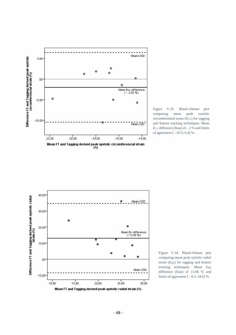
- 48 -
Figure V.34. Bland-Altman plot
comparing mean peak systolic radial
strain (ERR) for tagging and feature
tracking techniques. Mean ERR
difference (bias) of 13.06 % and
limits of agreement [– 8.5; 34.6] %.
Figure V.35. Bland-Altman plot
comparing mean peak systolic
circumferential strain (ECC) for tagging
and feature tracking techniques. Mean
ECC difference (bias) of – 2 % and limits
of agreement [ –10.5; 6.4] %.

- 49 -
Figure V.36. Comparison of CMR tagging versus
CMR FT derived peak systolic ERR in patients with
CoA or AvD.
Figure V.37. Comparison of CMR Tagging versus
CMR FT derived peak systolic ECC in patients with CoA
or AvD.
Figure V.39. Comparison of CMR FT derived peak
systolic ECC before and after treatment in patients with
CoA.
Figure V.38. Comparison of CMR FT derived peak
systolic ERR before and after treatment in patients with
CoA.

- 50 -
V.3. Discussion
In this part of the study, a recent FT approach was compared against the standard tagged images for
assessment of LV myocardial contractility, based on the analysis of radial and circumferential peak
systolic strains at the LV mid-level. Better agreement was obtained for the ECC parameter than for ERR.
These results are in concordance with previous studies. Hor et al showed that there is an excellent
agreement between the two techniques for estimating the ECC parameter in patients with DMD9 [42].
Augustine et al, which compared the two techniques in healthy volunteers, also focusing on ECC and ERR,
showed that the strongest agreement was obtained for the ECC and the result was better for the mid LV
slice [57]. ECC and ERR values were higher with FT than with tagging, Khan et al [7] also obtained the
same results for ECC.
It is known that myocardial fibers at the myocardium mid-wall are mostly circumferentially orientated
whilst those in the endocardium are mostly radially orientated [9]. This fact may explain why better
agreement was obtained for the ECC compared to the ERR as the measurements comprise the whole LV
myocardium at the mid-level slice. Schneeweis et al also stated that FT is a promising method to measure
ECC in patients with stenosis using medial and basal LV slices [10].
Several factors may have contributed to the differences between the two methods. The slice levels
chosen for tagging and those chosen for FT were similar but not identical; the two techniques have
different ways of measurement: HARP measures tag deformation of a myocardial segment within few
millimetres and FT tracks the motion of a tissue voxel. Furthermore, breath-hold requirements vary
among patients and between techniques and inadequacies of myocardium border delineation or tracking
may have contributed as well to the differences [61], [9]. The delineating inadequacies may result from
the need to contour manually both endocardial and epicardial borders based on a visual assessment.
Finally, according to Harrild et al [61], a reduced temporal resolution of CMR can interfere in the ability
to accurately measure peak systolic strains.
Regarding the strain evaluation in the CoA patients, the results suggested that both ECC and ERR values
were higher after treatment through graphical analysis but no statistical significance was reached.
Lossnitzer et al quantified the contractility patterns in patients with CoA and concluded that a significant
increase in ERR was verified after stent implantation [62]. A study from Kutty et al, which measured LV
myocardial strains (with CMR-FT) in repaired CoA presenting normal LV ejection fraction, suggests
that ERR is decreased and ECC maintained in comparison with healthy controls [63].
9 DMD – Duchenne muscular dystrophy

- 51 -
Advantages of FT against Tagging
In SSFP FT, acquisition time is reduced as myocardial tagging is not required and the analysis is
straightforward without the need for lengthy post-processing. FT is faster to analyse strains and tracks
myocardium more faithfully, and it can generate data four times more rapidly than tagging. [7], [9], [42]
Study Limitations
Limitations in this study are a reduced and not very homogenous sample (wide age range, unequal
number of men and women). Additionally, during the MR image acquisition, technical requirements
such as breath holding may have contributed to variability between acquisitions. Finally, as discussed
above, images used to measure the strains in tissue tagging are not always at the same levels than those
used for FT. If the same levels had been chosen, perhaps the results would have been more precise. As
stated in Taylor et al [56], it is extremely important to measure strain from the equivalent myocardial
layer anatomically so that the conditions for obtaining the results are as similar as possible.

- 52 -

- 53 -
VI. Conclusion
This work was carried out as part of an ongoing European Union project, which intends to evaluate the
applicability and effectiveness of predictive modelling and simulation tools for Cardiology, mainly, for
CoA and AvD conditions. As in many other diseases, evaluating and predicting relevant parameters is
fundamental to prevent further disease evolution or out of control situations. As such, it is necessary to
test assessment tools and evaluate clinical outcomes, most of the time by joining experts from a diverse
range of backgrounds.
This present work leads us to conclude that some functions of the WSS Explorer tool need further
improvement (for example, the calculation of the OSI parameter). As this was a preliminary use of the
program, this kind of improvements is expected sometimes.
Blood ejection fraction can be reduced in patients presenting CoA [64], thus it is important to evaluate
LV’s condition to prevent negative outcomes. Myocardium strain is more sensitive to contractile
dysfunctions than ejection parameter [41], thus, it is essential to determine LV anomalies and LV
remodelling after cardiovascular dysfunctions [52]. With this work and several previous studies, positive
results were produced regarding validating the FT technique against the standard Tagging technique by
using the ECC parameter.[65]
Given the obtained results, in future research, it should be possible to substitute tagging by FT as the
latter does not need additional MRI sequences and is less time consuming. Moreover, in the future,
additional developments and research need to be done concerning the estimation of myocardial radial
(ERR) and longitudinal (ELL) strains as the ECC is more related to LV short-axis function [64].
Additionally, research regarding strain rates could complement this work as strain rates seems to be
more sensitive than strain to myocardial pathology and to measure the LV contractility [66], [67]. Finally,
the results from the present work can have an impact to the ongoing and future projects related not only
to LV 3D remodelling but also to 3D heart modelling with the aim to forecast the evolution of the
diseases and to predict the most suitable intervention needed to treat them.

- 54 -

- 55 -
References
[1] “World Health Organization.” [Online]. Available: http://www.who.int/mediacentre/factsheets/fs317/en/.
[Accessed: 28-Aug-2016].
[2] “Cardioproof.” [Online]. Available: http://www.cardioproof.eu/about/overview-on-the-project/. [Accessed:
28-Aug-2016].
[3] J. LaDisa, R. Dholakia, and C. Figueroa, “Computational simulations demonstrate altered wall shear stress
(WSS) in aortic coarctation patients treated by resection with end-to-end anastomosis,” Congenit Heart Dis,
vol. 6, pp. 432–43, 2011.
[4] C. Meierhofer, E. Schneider, and C. Lyko, “Wall shear stress and flow patterns in the ascending aorta in
patients with bicuspid aortic valves differ significantly from tricuspid aortic valves: a prospective study,” Eur
Heart J Cardiovasc Imaging, 2012.
[5] E. Efstathopoulos, G. Patatoukas, and I. Pantos, “Wall shear stress calculation in ascending aorta, using phase
contrast magnetic resonance imaging. Investigating effective ways to calculate it in clinical practice,” Physica
Medica, vol. 24, pp. 175–181, 2008.
[6] E. Efstathopoulos, G. Patatoukas, and I. Pantos, “Measurement of systolic and diastolic arterial wall shear
stress in the ascending aorta,” Physica Medica, vol. 24, pp. 196–203, 2008.
[7] J. Khan, A. Singh, and S. Nazir, “Comparison of cardiovascular magnetic resonance feature tracking and
tagging for the assessment of left ventricular systolic strain in acute myocardial infarction,” vol. 17, no. suppl
1, p. 102, 2015.
[8] W. Moody, R. Taylor, and N. Edwards, “Comparison of magnetic resonance feature tracking for systolic and
diastolic strain and strain rate calculation with spatial modulation of magnetization imaging analysis,” J Magn
Reson Imaging, vol. 41, pp. 1000–12, 2015.
[9] L. Wu, T. Germans, and A. Güçlü, “Feature tracking compared with tissue tagging measurements of
segmental strain by cardiovascular magnetic resonance,” J Cardiovasc Magn Reson, vol. 16, p. 10, 2014.
[10] C. Schneeweis, T. Lapinskas, and B. Schnackenburg, “Comparison of myocardial tagging and feature tracking
in patients with severe aortic stenosis,” J Cardiovasc Magn Reson, vol. 15, no. supp1, p. 100, 2013.
[11] A. Guyton and J. Hall, Textbook of Medical Physiology, 11th ed. Elsevier Saunders, 2006.
[12] D. Ginat, M. Fong, and D. Tuttle, “Cardiac Imaging: Part I, MR Pulse Sequences, Imaging Planes, and Basic
Anatomy,” AJR, vol. 197, pp. 808–15, 2011.
[13] K. Saladin, Human Anatomy, 2nd ed. McGraw Hill, 2008.
[14] T. Forbes, D. Kim, and D. Turner, “Comparison of Surgical, Stent and Balloon Angioplasty Treatment of
Native Coarctation of the Aorta,” J Am Coll Cardiol, vol. 58, pp. 2664–74, 2011.
[15] R. Torok, M. Campbell, G. Fleming, and K. Hill, “Coarctation of the aorta: Management from infancy to
adulthood,” World J Cardiol, vol. 7, no. 11, pp. 765–75, 2015.
[16] D. Tanous, L. Benson, and E. Horlick, “Coarctation of the aorta: evaluation and management,” Current
Opinion in Cardiology, vol. 24, pp. 509–15, 2009.
[17] J. Lock, J. Bass, and K. Amplatz, “Balloon dilation angioplasty of aortic coarctations in infants and children,”
Circulation, vol. 68, pp. 109–16, 1983.

- 56 -
[18] M. OLaughlin, S. Perry, and J. Lock, “Use of endovascular stents in congenital heart disease,” Circulation,
vol. 83, pp. 1923–39, 1991.
[19] L. Pádua, L. Garcia, and C. Rubira, “Stent placement versus surgery for coarctation of the thoracic aorta,”
Cochrane Database Syst Rev, vol. 5, 2012.
[20] E. Riesenkampff, J. Fernandes, S. Meier, and L. Goubergrits, “Pressure Fields by Flow-Sensitive, 4D,
Velocity-Encoded CMR in Patients With Aortic Coarctation,” J Am Coll Cardiol Img, no. 7, pp. 920–6, 2014.
[21] “Congenital Heart Disease.” [Online]. Available: nlm.nih.gov/medlineplus/ency/article/001114.htm.
[Accessed: 10-Dec-2015].
[22] C. Westbrook and C. Kaut, MRI in Practice, 2nd ed. Blackwell Science, 1998.
[23] Z. Stankovic, B. Allen, and J. Garcia, “4D flow imaging with MRI,” Cardiovasc Diagn Ther, vol. 4, no. 2,
pp. 173–192, 2014.
[24] D. Pennell, “Cardiovascular Magnetic Resonance,” Circulation, vol. 121, pp. 692–705, 2010.
[25] F. Chan and K. Hanneman, “Computed Tomography and Magnetic Resonance Imaging in neonates with
congenital cardiovascular disease,” Semin Ultrasound CT MRI, vol. 36, no. 2, pp. 146–60, 2015.
[26] Y. Takehara, S. Yamashita, and H. Sakahara, “Magnetic Resonance Angiopraphy of the Aorta,” Ann Vasc
Dis, vol. 4, pp. 271–85, 2011.
[27] “Health Information for the Public.” [Online]. Available: www.nhlbi.nih.gov/health/health-topics. [Accessed:
12-Oct-2015].
[28] S. Singh and A. Goyal, “The origin of echocardiography: A Tribute to Inge Edler,” Tex Heart Inst J, vol. 34,
no. 4, pp. 431–438, 2007.
[29] M. Markl, A. Frydrychowicsz, and S. Kozerke, “4D Flow MRI,” J Magn Reson Imaging, vol. 36, pp. 1015–
36, 2012.
[30] M. Markl, “Velocity Encoding and Flow Imaging,” University Hospital Freiburg, Dept. of Diagnostic
Radiology, Medical Physics, Freiburg, Germany.
[31] A. Doltra, C. Schneeweis, and E. Fleck, “Cardiac magnetic resonance for prognostic assessment: present
applications and future directions,” Expert Rev Cardiosvasc Ther, vol. 12, no. 6, pp. 771–82, 2014.
[32] E. Ibrahim, “Myocardial tagging by Cardiovascular Magnetic Resonance: evolution of techniques-pulse
sequences, analysis algorithms, and applications,” J Cardiovasc Magn Reson, vol. 13, p. 36, 2011.
[33] A. Aletras, S. Ding, and R. Balaban, “DENSE: Displacement encoding with stimulated echoes in cardiac
functional MRI,” vol. 137, pp. 247–52, 1999.
[34] N. Osman, S. Sampath, and E. Atalar, “Imaging longitudinal cardiac strain on short-axis images using strain-
encoded MRI,” Magn Reson Med, vol. 46, pp. 324–34, 2001.
[35] M. Shehata, S. Cheng, and N. Osman, “Myocardial tissue tagging with cardiovascular magnetic resonance,”
vol. 11, p. 55, 2009.
[36] E. Zerhouni, D. Parish, and W. Rogers, “Human heart: tagging with MR imaging-a method for noninvasive
assessment of myocardial motion,” Radiology, vol. 169, pp. 59–63, 1988.
[37] L. Axel and L. Dougherty, “MR imaging of motion with spatial modulation of magnetization,” Radiology,
vol. 171, pp. 841–5, 1989.
[38] T. Mosher and M. Smith, “A DANTE tagging sequence for the evaluation of translational sample motion,”
Magn Reson Med, vol. 15, pp. 334–9, 1990.

- 57 -
[39] S. Fischer, G. McKinnon, and S. Maier, “Improved myocardial tagging contrast,” Magn Reson Med, vol. 30,
pp. 191–200, 1993.
[40] N. Osman, W. Kerwin, and E. McVeigh, “Cardiac motion tracking using CINE harmonic phase (HARP)
magnetic resonance imaging,” Magn Reson Med, vol. 42, pp. 1048–60, 1999.
[41] K. Hor, R. Baumann, and G. Pedrizzetti, “Magnetic resonance derived myocardial strain assessment using
feature tracking,” J Vis Exp, vol. 48, p. e2356, 2011.
[42] K. Hor, W. Gottliebson, and C. Carson, “Magnetic resonance feature tracking: comparison of feature tracking
method for strain calculation with harmonic phase imaging analysis,” JACC Cardiovasc Imaging, vol. 3, no.
2, pp. 152–4, 2010.
[43] A. Schuster, K. Hor, and J. Kowallick, “Cardiovascular Magnetic Resonance Myocardial Feature Tracking -
Concepts and Clinical Applications,” Circ Cardiovasc Imaging, 2016.
[44] T. Papaioannou and C. Stefanadis, “Vascular Wall Shear Stress: Basic Principles and Methods,” Hellenic J
Cardiol, vol. 46, pp. 9–15, 2005.
[45] J. Paszkowiak and A. Dardik, “Arterial wall shear stress: Observations from bench to bedside,” Vasc
Endovasc Surg, vol. 37, pp. 47–57, 2003.
[46] “Neointimal hyperplasia,” Medical Dictionary, 2009. [Online]. Available: http://medical-
dictionary.thefreedictionary.com/neointimal+hyperplasia. [Accessed: 25-Sep-2016].
[47] R. Gardhagen and K. Matts, “Wall shear stress in aorta with coarctation and post-stenotic dilatation,” in APS
Meeting Abstracts, 2012.
[48] J. Lantz, J. Renner, and M. Karlsson, “Wall shear stress in a subject specific human aorta - Influence of fluid-
structure interaction,” Int J Applied Mechanics, vol. 4, no. 3, pp. 759–778, 2011.
[49] F. Yin, “Ventricular wall stress,” Circ Res, vol. 49, pp. 829–42, 1981.
[50] A. Young, C. Kramer, and V. Ferrari, “Three-dimensional left ventricular deformation in hypertrophic
cardiomyopathy,” Circulation, vol. 90, no. 2, pp. 854–867, 1994.
[51] C. Moore, C. Lugo-Olivieri, and E. McVeigh, “Three-dimensional systolic strain patterns in the normal
human left ventricle: characterization with tagged MR imaging,” Radiology, vol. 214, no. 2, pp. 453–466,
2000.
[52]C. Hung, A. Verma, and H. Uno, “Longitudinal and Circumferential Strain Rate, Left Ventricular Remodeling,
and Prognosis After Myocardial Infarction,” vol. 56, no. 22, 2010.
[53] F. Callaghan, R. Kozor, and A. Sherrah, “Use of multi-velocity encoding 4D flow MRI to improve
quantification of flow patterns in the aorta,” J Magn Reson Imaging, vol. 43, no. 2, pp. 352–63, 2016.
[54] “Amira.” [Online]. Available: https://www.fei.com/software/amira-3d-for-life-sciences/. [Accessed: 15-Sep-
2016].
[55] H. Aguib, R. Torii, and Romeish, “Characterisation of spatiotemporal aortic flow and aortic wall
biomechanics in coarctation,” 45, 2015.
[56] R. Taylor, W. Moody, and F. Umar, “Myocardial strain measurement with feature-tracking cardiovascular
magnetic resonance: normal values,” Eur Heart J Cardiovasc Imaging, vol. 16, no. 8, pp. 871–81, Aug. 2015.
[57] D. Augustine, A. Lewandowski, and M. Lazdam, “Global and regional left ventricular myocardial
deformation measures by magnetic resonance feature tracking in healthy volunteers: comparison with tagging
and relevance of gender,” J Cardiovasc Magn Reson, vol. 15, p. 8, 2013.

- 58 -
[58] M. Cerqueira, J. Weissman, and V. Dilsizian, “Standardized Myocardial Segmentation and Nomenclature for
Tomographic Imaging of the Heart,” Circulation, vol. 105, no. 4, 2002.
[59] D. Giavarina, “Understanding Bland-Altman Analysis,” Biochemia Medica, vol. 25, no. 2, pp. 141–51, 2015.
[60] J. Bland and D. Altman, “Statistical methods for assessing agreement between two methods of clinical
measurement,” The Lancet, 1986.
[61] D. Harrild, Y. Han, and T. Geva, “Comparison of cardiac MRI tissue tracking and myocardial tagging for
assessment of regional ventricular strain,” Int J Cardiovasc Imaging, vol. 28, pp. 2009–18, 2012.
[62] D. Lossnitzer, H. Bellsham-Revell, and A. Bell, “Speckle tracking for cardiac MRI in patients pre and post
dilation and stent implantation of aortic coarctation,” J Cardiovasc Magn Reson, vol. 14, no. suppl 1, p. 125,
2012.
[63] S. Kutty, S. Rangamani, and J. Venkataraman, “Reduced global longitudinal and radial strain with normal
left ventricular ejection fraction late after effective repair of aortic coarctation: a CMR feature tracking study,”
J Cardiovasc Imaging, vol. 29, pp. 141–50, 2013.
[64] T. Leetmaa, B. Nørgaard, and H. Mølgaard, “Severe Aortic Coarctation in an Adult Patient with Normal
Brachial Blood Pressure,” J Clin Imaging Sci, vol. 4, no. 41, 2014.
[65] J. Park, D. Metaxas, and Q. Yuan, “Cascaded MRI-SPAMM for LV motion analysis during a whole cardiac
cycle,” vol. 55, no. 2, pp. 117–26, 1999.
[66] N. Greenberg, M. Firstenberg, and P. Castro, “Doppler-derived myocardial systolic strain rate is a strong
index of left ventricular contractility,” Circulation, vol. 105, pp. 99–105, 2002.
[67] J. Thomas and Z. Popovic, “Assessment of left ventricular function by cardiac ultrasound,” J Am Coll Cardiol,
vol. 48, pp. 2012–25, 2006.