i

Genetic analysis of heading cabbage traits

Performing a genome wide association study in a Brassica oleracea collection

Name: Twan Groot

Registration number: 921217285040

Supervisor: dr. ir. A.B. Bonnema

Examiners: dr. ir. A.B. Bonnema

P.F.P. Arens

March 2017

i

Copyright ©

Niets uit dit verslag mag worden verveelvoudigd en/of openbaar gemaakt door middel van

druk, fotokopie, microfilm of welke andere wijze ook, zonder voorafgaande schriftelijke

toestemming van de hoogleraar van de Labratory of Plant Breeding van Wageningen

Universiteit.

No part of this publication may be reproduced or published in any form or by any means,

electronic, mechanical, photocopying, recording or otherwise, without prior written permission

of the head of the Labratory of Plant Breeding of Wageningen University, The Netherlands.

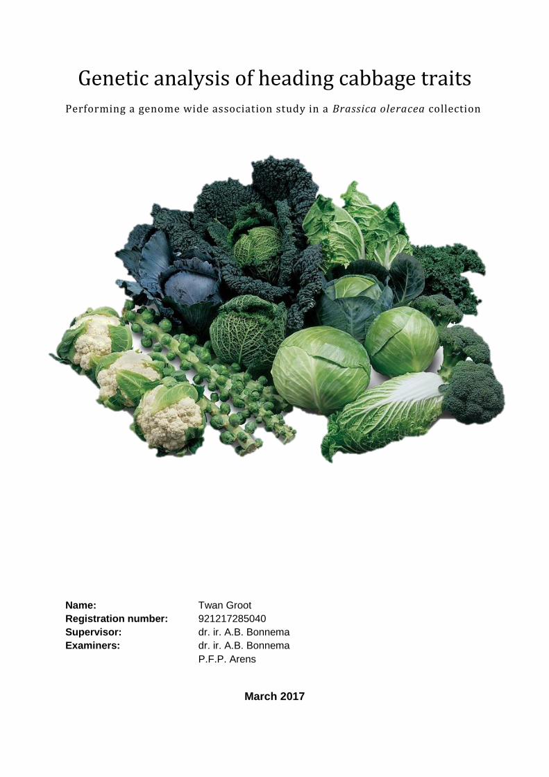
Front image:

VN plants (2017). VN Plants Plantenkwekerij – Mix naar eigen keuze. [online] Available at:

<https://www.vnplants.be/producten/kolen/assortiment/> [Accessed 19 March 2017]

ii

Wageningen University

Plant Breeding Department Growth and Development group

Genetic analysis of heading cabbage traits

Performing a genome wide association study in a Brassica oleracea collection

Name: Twan Groot

Registration number: 921217285040

Thesis code: PBR – 80436 | MSc Thesis Plant Breeding

Supervisor: dr. ir. A.B. Bonnema

Examiners: dr. ir. A.B. Bonnema

P.F.P. Arens

March 2017

iii

iv

Abstract

Brassica oleracea is an economically important plant species with a large variation in

morphotypes. The genetic regulation of leaf morphology is not fully understood. This study

focusses on the genetic basis behind the heading cabbage morphotype. First a population

structure was calculated over three iterations with 100.000 burn-in and 50.000 MCMC

calculations using STRUCTURE software. The result was a population structure with eight

subgroups. TASSEL software was used to calculate marker-trait associations. Three

phenotypic datasets, WURField2015, Companies2015 and ZonMW2016, served as

phenotypic input in the association analysis. Furthermore, genotypic data was gathered by

Sequence Based Genotyping, which resulted in 18.580 Single Nucleotide Polymorphisms.

TASSEL calculated many significant marker-trait associations after FDR correction. Due to

time constraints, interesting regions for Head Length, Blistering and Head Weight were

further analysed in the BolBase genome browser. A search window of 100 Kb around the

peak marker identified multiple candidate genes. Candidate genes of Head Length (CUC2),

Blistering (CYCU2-1, EXP4/6 and CUC1) and Head Weight (TMK1/4, APUM5, MKK5, GTE4

and CHC1) were proposed for further research.

v

Table of Contents 1. Introduction .................................................................................................................... 1

1.1. Brassicaceae and their ancestry .............................................................................. 1

1.2. Brassica oleracea .................................................................................................... 3

1.3. Leaf development .................................................................................................... 4

1.3.1. Leaf initiation .................................................................................................... 4

1.3.2. Adaxial/abaxial leaf polarity .............................................................................. 5

1.3.3. Cell growth: division and expansion ................................................................. 6

1.4. Current knowledge on leaf and heading traits in B. oleracea ................................... 7

1.5. GWAS and population structure .............................................................................. 8

2. Aim ................................................................................................................................. 9

3. Materials and methods ..................................................................................................10

3.1. Plant material .........................................................................................................10

3.2. Genomic data .........................................................................................................11

3.2.1. Sequence Based Genotyping ..........................................................................11

3.2.2. Population structure ........................................................................................11

3.2.3. GWAS .............................................................................................................12

3.3. Phenotypic data .....................................................................................................12

3.3.1. WURField2015 ................................................................................................13

3.3.2. Companies2015: Subset TKI 1000 genome project........................................13

3.3.3. ZonMW2016: ZonMW 3D Digileaf ...................................................................14

3.3.4. Statistical analysis ...............................................................................................16

4. Results ..........................................................................................................................17

4.1. Phenotypic data .....................................................................................................17

4.1.1. Companies2015 ..............................................................................................17

4.1.2. ZonMW 3D Digileaf .........................................................................................18

4.2. Population structure ...............................................................................................20

4.3. GWAS ....................................................................................................................21

4.4. Candidate genes ....................................................................................................24

5. Discussion .....................................................................................................................26

5.1. Phenotypic data .....................................................................................................26

5.1.1. Data quality .....................................................................................................26

5.1.2. Correlations within and between datasets .......................................................27

5.1.3. Differences between morphotypes ..................................................................28

5.2. Genotypic data .......................................................................................................31

5.2.1. Genotyping ......................................................................................................31

vi

5.2.2. Population structure ........................................................................................32

5.2.3. Genome wide association study ......................................................................34

5.2.4. Candidate genes .............................................................................................37

6. Conclusion and recommendations ................................................................................40

Acknowledgement ................................................................................................................41

References ...........................................................................................................................42

Appendix ..............................................................................................................................54

Appendix 1: Measured traits in WURField2015, Companies2015 and ZonMW2016 .........54

Appendix 1.1: Measured traits in WURField2015 ..........................................................54

Appendix 1.2: Measured traits in Companies2015 .........................................................55

Appendix 1.3: Definition of Head Shape parameters in ZonMW2016 ...........................56

Appendix 2: Heading cabbage definition by UPOV ...........................................................57

Appendix 3: Morphotypes and identification code .............................................................58

Appendix 4: Group definition population structure .............................................................58

Appendix 5: Phenotypic data analysis ZonMW2016..........................................................59

Appendix 5.1: ANOVA | Orientation effect block A .........................................................59

Appendix 5.2: ANOVA | Orientation effect block B .........................................................59

Appendix 5.3: ANOVA | Block effect ..............................................................................60

Appendix 5.4: ANOVA | Block*Genotype effect .............................................................61

Appendix 5.5: Pearson correlation matrix ......................................................................62

Appendix 5.6: Q-Q plots ZonMW2016 ...........................................................................62

Appendix 5.7: ANOVA | Traits per morphotype..............................................................63

Appendix 5.8: Boxplots ZonMW2016 .............................................................................66

Appendix 6: Phenotypic data analysis Companies2015 ....................................................67

Appendix 6.1: Pearson correlation matrix Companies2015 ...........................................67

Appendix 6.2: Q-Q plots Companies2015 .....................................................................68

Appendix 6.3: ANOVA | Traits per morphotype..............................................................69

Appendix 6.4: Boxplots Companies 2015 ......................................................................71

Appendix 7: GWAS ..........................................................................................................72

Appendix 7.1: Thresholds for GWAS per trait ................................................................72

Appendix 7.2: Manhattan plots WURField2015 .............................................................74

Appendix 7.3: Manhattan plots Companies2015............................................................76

Appendix 7.4: Manhattan plots ZonMW2016 .................................................................77

Appendix 7.5: Marker density ........................................................................................79

1

1. Introduction In this chapter, the Brassicaceae family and their ancestry is introduced. Furthermore, some

background about B. oleracea is given and followed up by knowledge on leaf growth. Finally,

genes associated with leafy head formation in cabbages are introduced.

1.1. Brassicaceae and their ancestry Brassica is a plant genus which is part of the Brassicaceae family and consists of 3709

species and 338 genera of which 308 can be assigned to 44 tribes (Warwick et al., 2006;

Warwick et al., 2010). Furthermore, cytogenetic studies confirmed large variation in

chromosome number for species within the Brassicaceae family ranging from four to 128

(Appel & Al-Shehbaz, 2003). The Brassicaceae family includes many widely cultivated crops.

Known products involve vegetable food, oil, condiments and animal feed (Cartea et al.,

2011). Furthermore, brassica is an economically important genus with a production of more

than 99 million tonnes of vegetable food and 70 million tonnes of oil and in 2013.

(FAOSTAT, 2015; Labana et al., 1993). Brassica vegetables are known for their nutritional

characteristics such as low fat and protein content, high amount of fibre, vitamins and

minerals. Besides the standard characteristics, brassicas possess glucosinolates which aid

the plant in defence against fungal and bacterial pathogens (Halkier & Gershenzon, 2006)

and have antioxidant and anticarcinogenic properties after consumption (Khwaja et al., 2009;

Li et al., 2010; Higdon et al., 2007).The six most important cultivated brassica species are

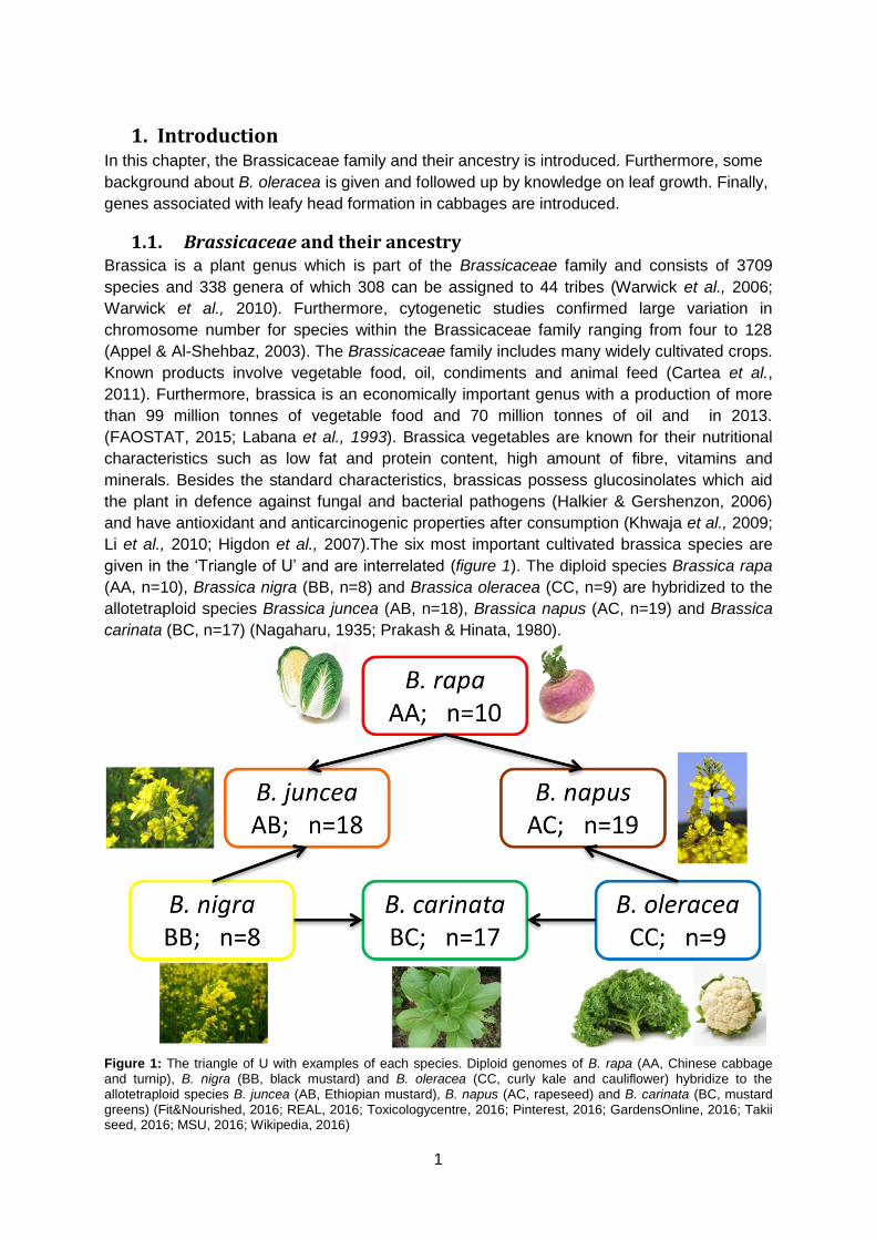
given in the ‘Triangle of U’ and are interrelated (figure 1). The diploid species Brassica rapa

(AA, n=10), Brassica nigra (BB, n=8) and Brassica oleracea (CC, n=9) are hybridized to the

allotetraploid species Brassica juncea (AB, n=18), Brassica napus (AC, n=19) and Brassica

carinata (BC, n=17) (Nagaharu, 1935; Prakash & Hinata, 1980).

Figure 1: The triangle of U with examples of each species. Diploid genomes of B. rapa (AA, Chinese cabbage and turnip), B. nigra (BB, black mustard) and B. oleracea (CC, curly kale and cauliflower) hybridize to the allotetraploid species B. juncea (AB, Ethiopian mustard), B. napus (AC, rapeseed) and B. carinata (BC, mustard greens) (Fit&Nourished, 2016; REAL, 2016; Toxicologycentre, 2016; Pinterest, 2016; GardensOnline, 2016; Takii seed, 2016; MSU, 2016; Wikipedia, 2016)

2

Many different morphotypes are present in each species and different organs are consumed

as vegetable (figure 1). For example, the floral organs of caixin (B. rapa) and cauliflower (B.

oleracea), the leafy head of cabbage (B. oleracea), Chinese cabbage (B. rapa) and head

mustard (B. juncea) and the tuberous parts of kohlrabi (B. oleracea), turnip (B. rapa) and

rutabaga (B. napus). Besides vegetables for consumption, vegetable oil can be extracted

from rapeseed (B. napus), sarsons (B. rapa) black mustard (B. nigra) and Indian mustard (b.

juncea. Furthermore, Indian mustard (B. juncea), black mustard (B. nigra) and the related

species white mustard (Sinapis alba), are used as condiment.

As can be seen in figure 1, different brassica species have different chromosome numbers.

B. rapa has ten pairs of chromosomes whereas B. oleracea has nine chromosome pairs. The

allopolyploid derived form of B. rapa and B. oleracea, B. napus contains the sum of their

chromosomes, 19 in total. Furthermore, 24 large genomic regions were identified, also

known as genomic blocks (GB). The GB are arranged in eight, nine or ten chromosomes and

are syntenic between genomes of Brassicaceae. (Cheng et al., 2014; Parkin et al., 2005;

Schranz et al., 2006; Lysak et al., 2007). Genomes of Brassicaceae that contain one set of

24 GB are considered diploid species whereas genomes with more than one set of 24 GB is

considered a paleopolyploid species (Cheng et al., 2014). The six species from ‘the triangle

of U’ share a whole genome triplication (WGT) event (Wang et al., 2011; Cheng et al., 2012;

Liu et al., 2014; Panjabi et al., 2014). This event took place after the divergence of the

brassica ancestor (translocation Proto-Calepineae Karyotype (tPCK)) and Arabidopsis

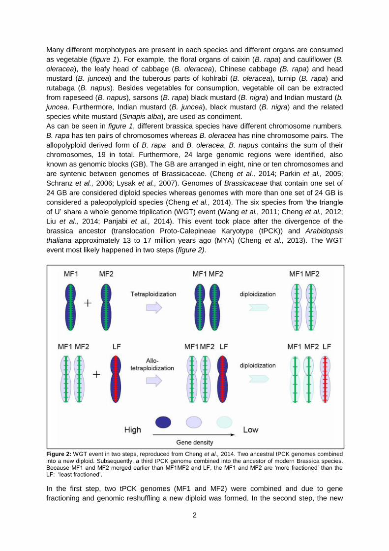
thaliana approximately 13 to 17 million years ago (MYA) (Cheng et al., 2013). The WGT

event most likely happened in two steps (figure 2).

Figure 2: WGT event in two steps, reproduced from Cheng et al., 2014. Two ancestral tPCK genomes combined

into a new diploid. Subsequently, a third tPCK genome combined into the ancestor of modern Brassica species. Because MF1 and MF2 merged earlier than MF1MF2 and LF, the MF1 and MF2 are ‘more fractioned’ than the LF: ‘least fractioned’.

In the first step, two tPCK genomes (MF1 and MF2) were combined and due to gene

fractioning and genomic reshuffling a new diploid was formed. In the second step, the new

3

diploid was combined with a third tPCK genome (LF). After a second round of gene

fractioning and genomic reshuffling the ancestor of Brassica was formed (Wang et al., 2011;

Cheng et al., 2012). The three subgenomes consist of the least fractionated subgenome (LF)

and the more fractionated subgenomes (MF1 and MF2). The LF subgenome is higher

expressed than the MF subgenomes, which resulted in more fractionation and thus gene loss

in the MF subgenomes. The LF subgenome has therefore more functional genes than the

MF subgenomes (Cheng et al., 2012). The WGT event and associated gene retention

contributed to the large variety of Brassica morphotypes (Cheng et al., 2016).

1.2. Brassica oleracea A species within the Brassica genus including many morphotypes is B. oleracea. B. oleracea

is a self-incompatible crop. Therefore, old races are heterogeneous due to open pollination.

However, modern hybrids are made from two homozygous parental lines which are crossed

to make a hybrid which is heterozygous on many loci with a homogeneous phenotype.

Debate has been going on about the origin of wild B. oleracea, also known as wild cabbage

(Smyth, 1995). The north Atlantic region was proposed (Song et al., 1980) versus the

Mediterranean region (Maggioni et al., 2010; Arias et al., 2014). The centres of domestication

and genetic diversity are in Europe and wild B. oleracea exist along the Atlantic and English

Channel coasts (Cartea et al., 2011; Bonnema et al., 2011). By the process of crop

domestication, various morphotypes were selected within this species (Gómez-Campo &

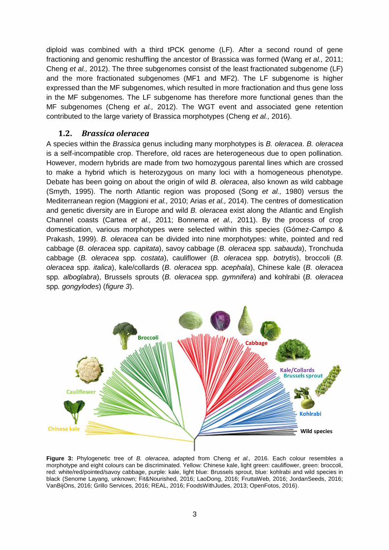
Prakash, 1999). B. oleracea can be divided into nine morphotypes: white, pointed and red

cabbage (B. oleracea spp. capitata), savoy cabbage (B. oleracea spp. sabauda), Tronchuda

cabbage (B. oleracea spp. costata), cauliflower (B. oleracea spp. botrytis), broccoli (B.

oleracea spp. italica), kale/collards (B. oleracea spp. acephala), Chinese kale (B. oleracea

spp. alboglabra), Brussels sprouts (B. oleracea spp. gymnifera) and kohlrabi (B. oleracea

spp. gongylodes) (figure 3).

Figure 3: Phylogenetic tree of B. oleracea, adapted from Cheng et al., 2016. Each colour resembles a

morphotype and eight colours can be discriminated. Yellow: Chinese kale, light green: cauliflower, green: broccoli, red: white/red/pointed/savoy cabbage, purple: kale, light blue: Brussels sprout, blue: kohlrabi and wild species in black (Senome Layang, unknown; Fit&Nourished, 2016; LaoDong, 2016; FruttaWeb, 2016; JordanSeeds, 2016; VanBijOns, 2016; Grillo Services, 2016; REAL, 2016; FoodsWithJudes, 2013; OpenFotos, 2016).

4

Different plant organs are consumed for many of these morphotypes. Inflorescence are

consumed for broccoli and cauliflower whereas the swollen stem is consumed for kohlrabi

and axillary buds for Brussels sprouts. Furthermore, leafs are consumed for kale and

Chinese kale. Besides loose leafs, folded leaves form a head which is the consumed part of

cabbage (Bonnema et al., 2011). A large variation in leaf shape, colour, size and texture is

observed when all morphotypes are compared with each other. Furthermore, leaves can aid

the crop in improving the quality of edible parts. For instance: the inward folding leaves of

cauliflower protect the curd from physical damage and ensures the white colour of the curd

by blocking sunlight. Therefore, breeders aim to improve these traits in their crops. However,

the genetic regulation of leaf morphology of B. oleracea is not fully understood. It is still

unknown why certain morphotypes form heads whereas others form a rosette. This makes

leaf traits and the genetics behind them interesting to study.

1.3. Leaf development Plant leaves determine the light capturing area, sense light spectra, temperature, host-plant

interactions, tolerance to abiotic stress and day length (Dhkar & Pareek, 2014). To reach a

better understanding in leaf morphology, leaf traits should be studied and therefore leaf

development is an important starting point. Leaf development is well studied in model

species A. thaliana, a family member of the Brassicaceae family. Leaf development starts in

the shoot apical meristem (SAM) where stem cells lose their identity. This is followed by leaf

initiation by formation of the leaf primordium. The adaxial/abaxial sides of the leaf are

determined by leaf polarity control. Furthermore, leaf width and length are defined by leaf

polarity control genes. Subsequently, leaf growth is driven by cytoplasmic growth, cell

division and cell expansion. Finally, cell differentiation causes cells to form stomata, vascular

tissue or trichomes. The different developmental stages are controlled by various regulatory

pathways having hormonal and genetic compounds (Braybrook & Kuhlemeier, 2010; Kalve et

al., 2014; Bar & Ori, 2014).

1.3.1. Leaf initiation

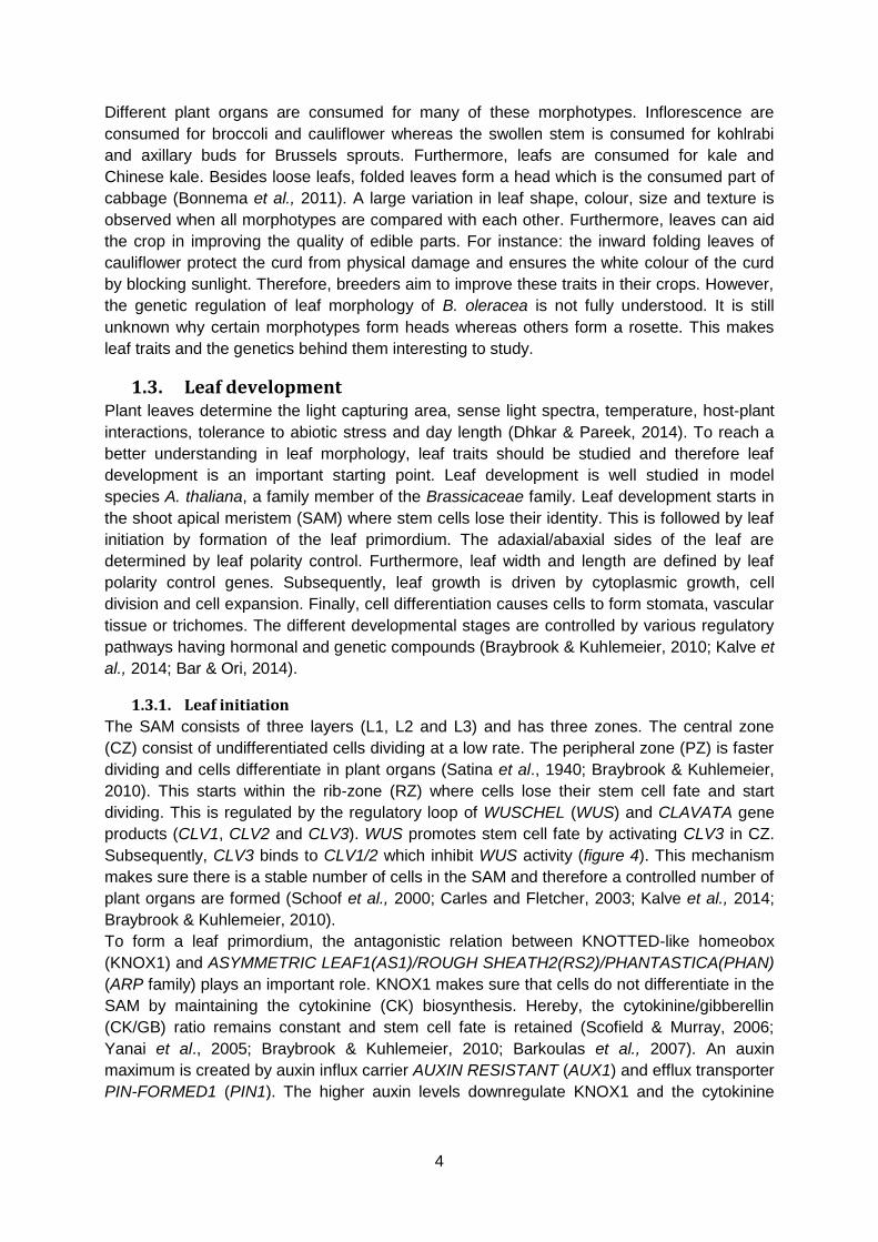
The SAM consists of three layers (L1, L2 and L3) and has three zones. The central zone

(CZ) consist of undifferentiated cells dividing at a low rate. The peripheral zone (PZ) is faster

dividing and cells differentiate in plant organs (Satina et al., 1940; Braybrook & Kuhlemeier,

2010). This starts within the rib-zone (RZ) where cells lose their stem cell fate and start

dividing. This is regulated by the regulatory loop of WUSCHEL (WUS) and CLAVATA gene

products (CLV1, CLV2 and CLV3). WUS promotes stem cell fate by activating CLV3 in CZ.

Subsequently, CLV3 binds to CLV1/2 which inhibit WUS activity (figure 4). This mechanism

makes sure there is a stable number of cells in the SAM and therefore a controlled number of

plant organs are formed (Schoof et al., 2000; Carles and Fletcher, 2003; Kalve et al., 2014;

Braybrook & Kuhlemeier, 2010).

To form a leaf primordium, the antagonistic relation between KNOTTED-like homeobox

(KNOX1) and ASYMMETRIC LEAF1(AS1)/ROUGH SHEATH2(RS2)/PHANTASTICA(PHAN)

(ARP family) plays an important role. KNOX1 makes sure that cells do not differentiate in the

SAM by maintaining the cytokinine (CK) biosynthesis. Hereby, the cytokinine/gibberellin

(CK/GB) ratio remains constant and stem cell fate is retained (Scofield & Murray, 2006;

Yanai et al., 2005; Braybrook & Kuhlemeier, 2010; Barkoulas et al., 2007). An auxin

maximum is created by auxin influx carrier AUXIN RESISTANT (AUX1) and efflux transporter

PIN-FORMED1 (PIN1). The higher auxin levels downregulate KNOX1 and the cytokinine

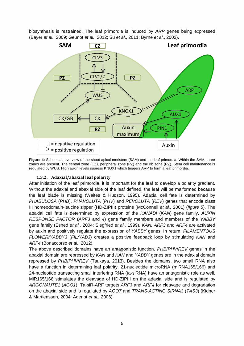
5

biosynthesis is restrained. The leaf primordia is induced by ARP genes being expressed

(Bayer et al., 2009; Geunot et al., 2012; Su et al., 2011; Byrne et al., 2002).

Figure 4: Schematic overview of the shoot apical meristem (SAM) and the leaf primordia. Within the SAM, three

zones are present. The central zone (CZ), peripheral zone (PZ) and the rib zone (RZ). Stem cell maintenance is regulated by WUS. High auxin levels supress KNOX1 which triggers ARP to form a leaf primordia.

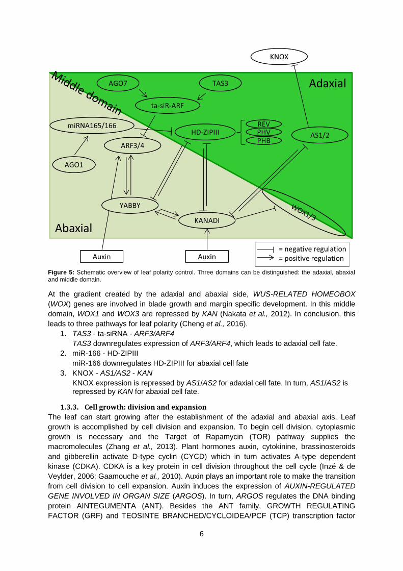
1.3.2. Adaxial/abaxial leaf polarity

After initiation of the leaf primordia, it is important for the leaf to develop a polarity gradient.

Without the adaxial and abaxial side of the leaf defined, the leaf will be malformed because

the leaf blade is missing (Waites & Hudson, 1995). Adaxial cell fate is determined by

PHABULOSA (PHB), PHAVOLUTA (PHV) and REVOLUTA (REV) genes that encode class

III homeodomain-leucine zipper (HD-ZIPIII) proteins (McConnell et al., 2001) (figure 5). The

abaxial cell fate is determined by expression of the KANADI (KAN) gene family, AUXIN

RESPONSE FACTOR (ARF3 and 4) gene family members and members of the YABBY

gene family (Eshed et al., 2004; Siegfried et al., 1999). KAN, ARF3 and ARF4 are activated

by auxin and positively regulate the expression of YABBY genes. In return, FILAMENTOUS

FLOWER/YABBY3 (FIL/YAB3) creates a positive feedback loop by stimulating KAN and

ARF4 (Bonaccorso et al., 2012).

The above described domains have an antagonistic function. PHB/PHV/REV genes in the

abaxial domain are repressed by KAN and KAN and YABBY genes are in the adaxial domain

repressed by PHB/PHV/REV (Tsukaya, 2013). Besides the domains, two small RNA also

have a function in determining leaf polarity. 21-nucleotide microRNA (miRNA165/166) and

24-nucleotide transacting small interfering RNA (ta-siRNA) have an antagonistic role as well.

MiR165/166 stimulates the cleavage of HD-ZIPIII on the adaxial side and is regulated by

ARGONAUTE1 (AGO1). Ta-siR-ARF targets ARF3 and ARF4 for cleavage and degradation

on the abaxial side and is regulated by AGO7 and TRANS-ACTING SIRNA3 (TAS3) (Kidner

& Martienssen, 2004; Adenot et al., 2006).

6

Figure 5: Schematic overview of leaf polarity control. Three domains can be distinguished: the adaxial, abaxial

and middle domain.

At the gradient created by the adaxial and abaxial side, WUS-RELATED HOMEOBOX

(WOX) genes are involved in blade growth and margin specific development. In this middle

domain, WOX1 and WOX3 are repressed by KAN (Nakata et al., 2012). In conclusion, this

leads to three pathways for leaf polarity (Cheng et al., 2016).

1. TAS3 - ta-siRNA - ARF3/ARF4

TAS3 downregulates expression of ARF3/ARF4, which leads to adaxial cell fate.

2. miR-166 - HD-ZIPIII

miR-166 downregulates HD-ZIPIII for abaxial cell fate

3. KNOX - AS1/AS2 - KAN

KNOX expression is repressed by AS1/AS2 for adaxial cell fate. In turn, AS1/AS2 is repressed by KAN for abaxial cell fate.

1.3.3. Cell growth: division and expansion

The leaf can start growing after the establishment of the adaxial and abaxial axis. Leaf

growth is accomplished by cell division and expansion. To begin cell division, cytoplasmic

growth is necessary and the Target of Rapamycin (TOR) pathway supplies the

macromolecules (Zhang et al., 2013). Plant hormones auxin, cytokinine, brassinosteroids

and gibberellin activate D-type cyclin (CYCD) which in turn activates A-type dependent

kinase (CDKA). CDKA is a key protein in cell division throughout the cell cycle (Inzé & de

Veylder, 2006; Gaamouche et al., 2010). Auxin plays an important role to make the transition

from cell division to cell expansion. Auxin induces the expression of AUXIN-REGULATED

GENE INVOLVED IN ORGAN SIZE (ARGOS). In turn, ARGOS regulates the DNA binding

protein AINTEGUMENTA (ANT). Besides the ANT family, GROWTH REGULATING

FACTOR (GRF) and TEOSINTE BRANCHED/CYCLOIDEA/PCF (TCP) transcription factor

7

families regulate cell growth (Hu et al., 2003; Kalve et al., 2014). GRF5 has an interaction

with GRF-INTERACTING FACTOR1 (GIF1) and both are negatively regulated by miR396.

Subsequently, CINCINNATA (CIN-TCP) negatively regulates miR396 and is involved in a cell

cycle checkpoint (Horiguchi et al., 2005; Liu et al., 2009; Rodriguez et al., 2010; Platnik et al.,

2003). Besides transcription factors, multiple genes play a role in cell expansion. The

putative ubiquitin receptor DA1, that restricts cell proliferation, and E3 ubiquitin ligase BIG

BROTHER, that limits organ size, are restricting the duration of cell growth. Furthermore,

DA1 cooperates with mediator complex subunit 25 (MED25) to restrict cell growth (Li et al.,

2008; Xu & Li, 2011). KLUH (KLU/CYP78A5) is a regulator of leaf size control (Anastasiou et

al., 2007). Moreover, STRUWWELPETER (SWP) has a function in defining the period of cell

growth and acts similar to MED25 (Autran et al., 2002). For cell expansion, the cell wall is

loosened by various proteins and this process is vacuole and turgor driven (Scheuring et al.,

2016). Auxin and brassinoline, a brassinosteroid, induce the activity of P-type plasma

membrane proton ATPase (AHA). In turn, AHA activates expansins (EXP),

xyloglucanendotransglucosylase/hydrolase (XTH), xyloglucan endohydrolase (XEH) and

xyloglucan endotransglucosylase (XET) which results in cell wall loosening (Wolf et al., 2012;

Yokoyama & Nishitani, 2001). Genes that are possibly related to cell expansion are

ANGUSTIFOLIA (AN3), ROTUNDIFOLIA3 (ROT3) and JAGGED (JAG) (Horiguchi et al.,

2011; Tsunge et al., 1996; Dinneny et al., 2004).

The final step in the development of a leaf is cell differentiation. Main groups are defined as

guard cells, vascular tissue and trichomes. Each of these types have separate genetic

pathways which are extensively described in Kalve et al., 2014.

1.4. Current knowledge on leaf and heading traits in B. oleracea The knowledge of leaf development, mainly obtained in A. thaliana, as described in the

previous paragraphs can be applied to study leaf development of another member of the

Brassicaceae family: B. oleracea. Few studies have been conducted on leaf morphology in

Brassica’s. Lan and Paterson, 2001 looked at the F2 population derived from crosses

between rapid cycling B. oleracea and three cauliflower varieties: Cantanese, Pusa Katki and

Bugh Kana. Traits were correlated to quantitative trait loci (QTLs). However, the WTL have

not been fine-mapped and genes underlying the traits were not discovered. In another

research project from Sebastian et al., 2002, Brussel sprouts were crossed to cauliflower.

Leaf, flowering, axillary bud and stem traits were correlated to QTL regions but no genes

were identified.

In a recent study conducted by the Brassica groups of Wageningen Plant Breeding and the

Institute of Vegetables of Flowers of the Chinese Academy of Agricultural Sciences, genome

resequence data from many genotypes were compared to identify regions of selection for

leafy head formation in cabbages. They identified three candidate genes for leaf heading

traits: BoATHB15.2, BoKAN2.2 and BoBRX.2. BoATHB15.2 is an orthologue of

ARABIDOPSIS HOMEOBOX 15 and belongs to the HD-ZIPIII gene family. Furthermore,

BoKAN2.2 is an orthologue of the KANADI gene family and BoBRX.2 is an orthologue of

BREVIS RADIX (BRX). BRX plays a role in auxin signalling, brassinosteroid biosynthesis

and cytokinine signalling which regulates cell growth and cell size (Mouchel et al., 2006; Li et

al., 2009). In addition to B. oleracea, Cheng et al., 2016 found either orthologues of these

candidate genes or other genes in the same molecular pathway in B. rapa. Genes from the

ARF family were found besides KAN and BRX genes.

It is likely that leaf polarity genes play an important role in differentiating heading B. oleracea

from other B. oleracea crop types. Knowledge on leaf formation and leaf growth has been

8

studies extensively in A. thaliana. However, little knowledge on leafy head formation, in for

example cabbage (B. oleracea), Chinese cabbage (B. rapa) and lettuce (Lactuca sativa)

exists. Leafy head formation is a clear domestication trait and is therefore interesting to

study. An approach to identify possible genes is a genome wide association study (GWAS).

In addition, leaf formation and regulation has to be studied and accurately described to

define traits than can be used in an association analysis.

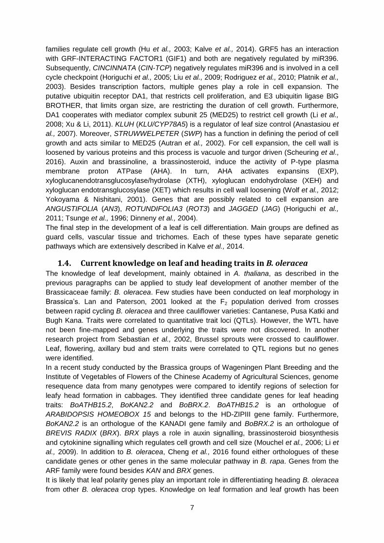
1.5. GWAS and population structure A genomic wide association study is an association analysis that can link a phenotypic trait to

a location on the genome in large collections of genotypes belonging to a species. An

important aspect of this method is that allelic variation is distributed over the genome.

Furthermore, prior knowledge about regions or genes is not necessary since a GWAS will

identify regions linked to the trait of interest. Association analysis uses the natural variation

and historical recombination of the mapping populations (Nordborg & Tavaré, 2002; Risch &

Merikangas, 1996). Therefore, it is important to have a sufficient large sample population that

effectively provides genetically information (Cantor et al., 2010).

In this study, the mapping population consists of many accessions representing various

morphotypes of B. oleracea. The B. oleracea population is not homogeneous because

breeding efforts occurred more within morphotypes than between morphotypes. The

breeding efforts resulted in a population structure which can lead to false positives.

Especially, when the variation of the trait of interest is strongly associated with a

subpopulation. Therefore, it is important to correct the GWAS with a population structure to

reduce false positives. A population structure uses allelic information from random molecular

markers across the genome to account for genetic relatedness in an association analysis

(Zhu et al., 2008). When false positives are accounted for, overcorrection can cause the

introduction of false negatives. This is caused by the removal of candidate genes associated

with the morphological trait and the population structure. Figure 6 gives an overview of the

steps to perform a GWAS. The germplasm has to be grown to phenotype certain traits.

Additionally, germplasm has to be genotyped, for example by sequencing. After sequencing,

genome-wide polymorphisms can be called and a population structure can be made. The

phenotypic and genotypic data can be combined for association analysis in various

association analysis software.

Figure 6: Overview of GWAS adapted from Zhu et al., 2008. The association analysis is performed by finding

associations between the phenotype (Y) and the genotype (G) corrected with population structure (Q) and/or kinship correction (K). Residual variance (E) also plays a role in finding associations.

9

2. Aim The aim of this thesis will be to study the genetic basis behind leaf morphology in B. oleracea

and in particular the heading cabbage morphotype. This will be done by performing a GWAS

on a collection of B. oleracea, representing all morphotypes and consisting of modern

hybrids, old landraces and wild species. In order to do so, genotypic data obtained by SBG

has to be analysed to call Single Nucleotide Polymorphisms that serve as input to build a

population structure and for the association analysis. Furthermore, multiple phenotypic

datasets have to be collected and analysed to serve as input for the association analysis.

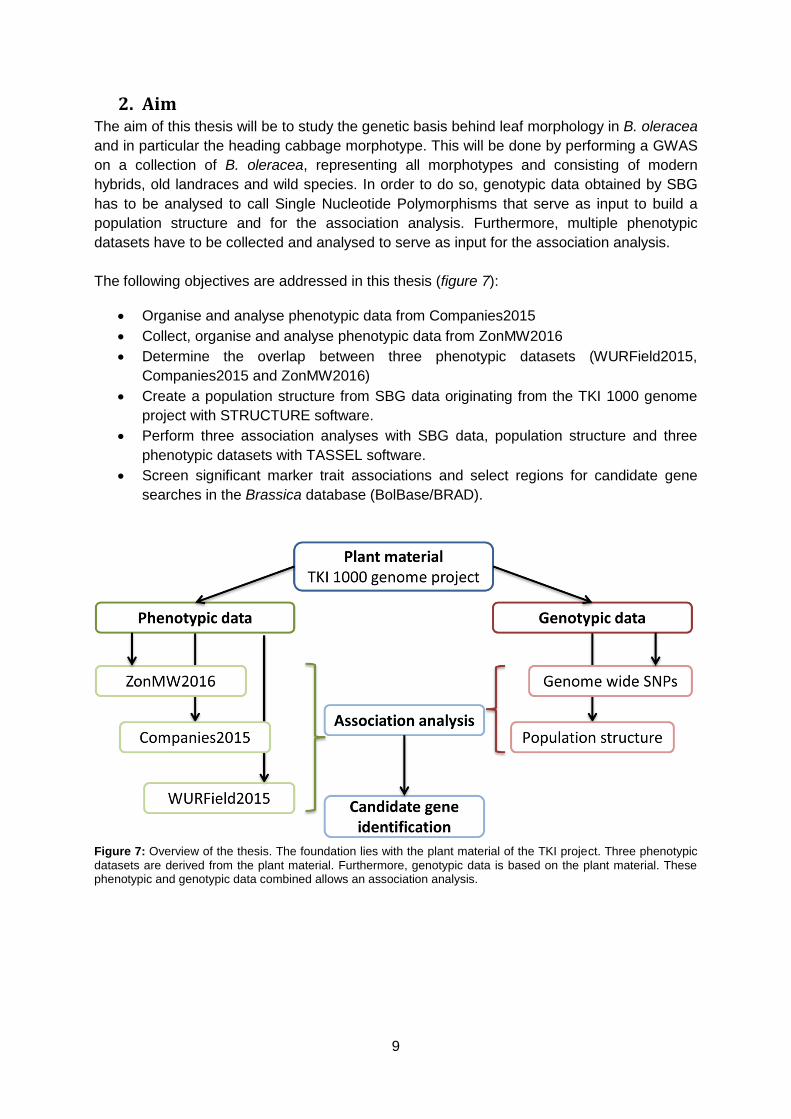
The following objectives are addressed in this thesis (figure 7):

Organise and analyse phenotypic data from Companies2015

Collect, organise and analyse phenotypic data from ZonMW2016

Determine the overlap between three phenotypic datasets (WURField2015,

Companies2015 and ZonMW2016)

Create a population structure from SBG data originating from the TKI 1000 genome

project with STRUCTURE software.

Perform three association analyses with SBG data, population structure and three

phenotypic datasets with TASSEL software.

Screen significant marker trait associations and select regions for candidate gene

searches in the Brassica database (BolBase/BRAD).

Figure 7: Overview of the thesis. The foundation lies with the plant material of the TKI project. Three phenotypic

datasets are derived from the plant material. Furthermore, genotypic data is based on the plant material. These phenotypic and genotypic data combined allows an association analysis.

10

3. Materials and methods All data, genomic and phenotypic, originate from a TKI project: 1000 B. oleracea genomes

which started in 2015. The project has the goal to genotype 1000 different B. oleracea

genomes to reveal the genetic diversity in modern hybrids, genebank accessions and wild

accessions across different morphotypes. The group of Guusje Bonnema is cooperating in

this project with 7 other companies. Bejo, Hazera, Rijk Zwaan, Syngenta, Enza and Takii as

breeding companies and KeyGene as molecular marker provider. For the genomic data,

Sequence based genotyping (SBG) was performed and was used to determine the

population structure. Furthermore, it served as genomic input for the GWAS. Three

phenotypic datasets were collected in multiple years on multiple sites which served as input

for the GWAS.

3.1. Plant material In the TKI 1000 genomes project, 936 unique modern hybrids (380) and genebank material

(556) which consist of landraces and wild material were send for genotyping. For the ease of

communication the modern hybrids, landraces and wild material will be called accessions. In

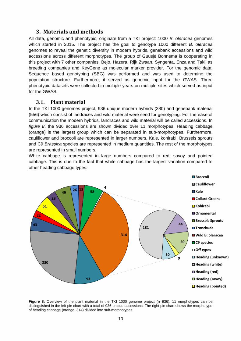
figure 8, the 936 accessions are shown divided over 11 morphotypes. Heading cabbage

(orange) is the largest group which can be separated in sub-morphotypes. Furthermore,

cauliflower and broccoli are represented in larger numbers. Kale, kohlrabi, Brussels sprouts

and C9 Brassica species are represented in medium quantities. The rest of the morphotypes

are represented in small numbers.

White cabbage is represented in large numbers compared to red, savoy and pointed

cabbage. This is due to the fact that white cabbage has the largest variation compared to

other heading cabbage types.

Figure 8: Overview of the plant material in the TKI 1000 genome project (n=936). 11 morphotypes can be

distinguished in the left pie chart with a total of 936 unique accessions. The right pie chart shows the morphotype of heading cabbage (orange, 314) divided into sub-morphotypes.

93

230

43

22

51

28

49 26 18

58 4

30

181 44

50

9

314

Broccoli

Cauliflower

Kale

Collard Greens

Kohlrabi

Ornamental

Brussels Sprouts

Tronchuda

Wild B. oleracea

C9 species

Off types

Heading (unknown)

Heading (white)

Heading (red)

Heading (savoy)

Heading (pointed)

11

3.2. Genomic data In this section, the genotypic data will be explained. SBG was performed on the plant

material described above. For hybrids, which are homogeneous, DNA was isolated from the

hypocotyls and cotyledons of 50-100 seedlings. For genebank accessions and accessions

representing wild Brassica’s, DNA was isolated from single plants representing the

heterogeneous accession. After processing by a bioinformatician, this genotypic data served

as input for a population structure and subsequent association analysis.

3.2.1. Sequence Based Genotyping

Sequence based genotyping is a genotyping method developed by KeyGene N.V. A genome

reduction step is performed by cutting the genome with two restriction enzymes. PstI (5’-

CTGCA/G-3’) and MseI (5’-T/TAA-3’) were chosen to cut the DNA which have a recognition

site of six and four nucleotides long. Furthermore, two selective nucleotides (GC) were

attached to the MseI end to control the amount of cuts made. The fragment flanked by PstI-

MseI sites plus the two selective nucleotides was sequenced from the PstI site by Illumina

sequencing resulting in sequence data with an approximate length of 120 base pairs.

SEED software was used for variant calling on the Binary Alignment/Map (BAM) files. Loci

were selected that occur in at least 800 of the 1008 accessions and have at least two reads

coverage. Only Single Nucleotide Polymorphism (SNPs) were retained, InDels were not

considered for this analysis. The reads with a mapping quality of five or higher were mapped

to a unique location on reference genome of homozygous white cabbage line 02-12 (Liu et

al., 2014) by Theo Borm. The reads mapped to nine chromosomes representing the genome

of B. oleracea with a length of approximately 500 Mb. The reads that did not map to the

reference genome were assigned to fictional chromosome C00 with three times ‘N’ between

reads. The germplasm contained duplicates for a diversity panel which were removed after

mapping. This resulted in a dataset of 85.532 loci (SNPs) in 943 accessions in Variant Call

Format (VCF).

The dataset is filtered with a genotype call of 80% which resulted in 85.168 remaining loci.

Furthermore, a minor allele frequency (MAF) was chosen of 2.5% which resulted in 18.580

loci with an allele frequency > 2.5 %. Accessions with more than 60% missing values were

removed from the dataset. This dataset with 18.580 loci in 913 accessions will be used as

genotypic input for the association analysis. To calculate a population structure, the dataset

was thinned to have a reasonable computational time. Loci were selected with ≥ 250 Kb

distance. This resulted in 1376 SNP markers evenly distributed over the genome with an

average distance of 0.36 Mb.

3.2.2. Population structure

The population structure was calculated using the 913 accessions and SNP markers

described in section 3.1.1. However, due to time and computational limitations 459 SNP

markers were used to calculate a population structure. The population structure program

STRUCTURE 2.3.4 (Pritchard et al., 2002) was used to perform the calculations. The SNPs

were converted from VCF to STRUCTURE format using PGDSpider 2.1.0.3 (Lischer &

Excoffier, 2012). PGDSpider was run with only SNP markers and the numeric format has five

values: 1 for Guanine, 2 for Cytosine, 3 for Tyrosine, 4 for Adenine and -9 for a missing

value.

STRUCTURE was run with a burnin period of 100.000 runs followed up by 50.000 Markov

chain Monte Carlo (MCMC) calculations. All calculations were performed three times with the

assumption of two to 12 subpopulations (K). The optimal number of subpopulations was

12

determined by StructureHarvester (Earl, 2012; Evanno et al., 2005). In StructureHarvester,

four graphs are shown:

1. L(K) The likelihood per K Pritchard et al., 2002

2. L’(K) The first rate of change of L(K) Evanno et al., 2005

3. |L’’(K)| The second rate of change of L’(K) Evanno et al., 2005

4. ∆K |L’’(K)| / StDev(L(K)) Evanno et al., 2005

In the first graph from Pritchard et al., 2002, a plateau could indicate the optimal K and is

calculated by: 𝑂𝑝𝑡𝑖𝑚𝑎𝑙 𝐾 = (𝐾 𝑎𝑡 𝑝𝑙𝑎𝑡𝑒𝑎𝑢) − 1

Furthermore, the fourth graph (∆K) shows a peak at the optimal K. When an optimal K was

chosen, the Q matrices from three iterations were compared for data consistency. The goal

is to verify if each accession was assigned to the same K. One Q matrix is selected and

served as input for the association analysis. Furthermore, STRUCTURE provides bar plots to

visualize the results. Q matrix values ≥ 50% were used for the description of the composition

of the different populations (K).

3.2.3. GWAS

The association analysis was performed with TASSEL software version 5.2.33 (Bradbury et

al., 2007). A General Linear Model (GLM) was chosen to calculate marker-trait associations.

The model requires two or three input files. Genotypic data: described in section 3.2.1, an

optional population structure: described in section 3.2.2 and phenotypic data: described in

paragraph 3.3. The GLM was run with 999 permutations to control the experiment-wise error

rate for individual phenotypes (Anderson & ter Braak, 2003). Significant marker-trait

associations were determined by the False Discovery Rate (FDR) (Benjamini & Hochberg,

1995; Pike, 2011). The FDR threshold was set at 0.01 which lead to a significant marker-trait

association when the q-value ≤ 0.01. Significant associations were visualized by Manhattan

plots. From these Manhattan plots, markers were selected that increase in LOD score when

we compare the GWAS without and with population structure respectively. Furthermore,

markers that are associated with a trait in multiple datasets have a higher possibility to be

truly associated. Candidate regions were investigated in BolBase (Yu et al., 2013).

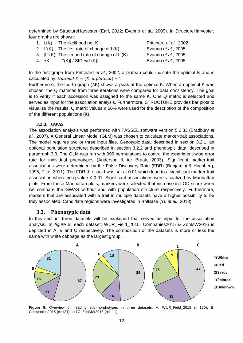
3.3. Phenotypic data In this section, three datasets will be explained that served as input for the association

analysis. In figure 9, each dataset: WUR_Field_2015, Companies2015 & ZonMW2016 is

depicted in A, B and C respectively. The composition of the datasets is more or less the

same with white cabbage as the largest group.

Figure 9: Overview of heading sub-morphotypes in three datasets. A: WUR_Field_2015 (n=160), B:

Companies2015 (n=121) and C: ZonMW2016 (n=111)

47

29

25

9

1

White

Red

Savoy

Pointed

Unknown

59

16

29

4 13

87

21

16

5

31

A B C

13

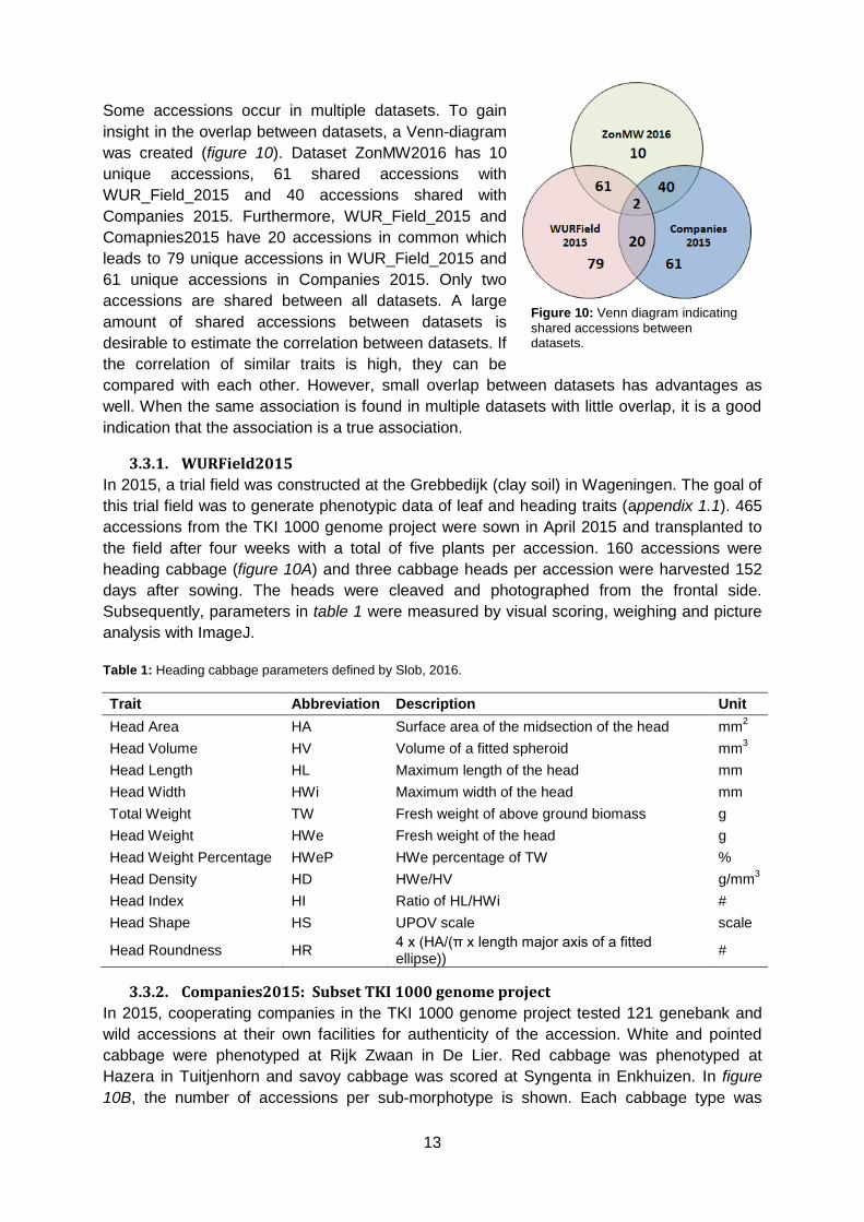
Some accessions occur in multiple datasets. To gain

insight in the overlap between datasets, a Venn-diagram

was created (figure 10). Dataset ZonMW2016 has 10

unique accessions, 61 shared accessions with

WUR_Field_2015 and 40 accessions shared with

Companies 2015. Furthermore, WUR_Field_2015 and

Comapnies2015 have 20 accessions in common which

leads to 79 unique accessions in WUR_Field_2015 and

61 unique accessions in Companies 2015. Only two

accessions are shared between all datasets. A large

amount of shared accessions between datasets is

desirable to estimate the correlation between datasets. If

the correlation of similar traits is high, they can be

compared with each other. However, small overlap between datasets has advantages as

well. When the same association is found in multiple datasets with little overlap, it is a good

indication that the association is a true association.

3.3.1. WURField2015

In 2015, a trial field was constructed at the Grebbedijk (clay soil) in Wageningen. The goal of

this trial field was to generate phenotypic data of leaf and heading traits (appendix 1.1). 465

accessions from the TKI 1000 genome project were sown in April 2015 and transplanted to

the field after four weeks with a total of five plants per accession. 160 accessions were

heading cabbage (figure 10A) and three cabbage heads per accession were harvested 152

days after sowing. The heads were cleaved and photographed from the frontal side.

Subsequently, parameters in table 1 were measured by visual scoring, weighing and picture

analysis with ImageJ.

Table 1: Heading cabbage parameters defined by Slob, 2016.

Trait Abbreviation Description Unit

Head Area HA Surface area of the midsection of the head mm2

Head Volume HV Volume of a fitted spheroid mm3

Head Length HL Maximum length of the head mm

Head Width HWi Maximum width of the head mm

Total Weight TW Fresh weight of above ground biomass g

Head Weight HWe Fresh weight of the head g

Head Weight Percentage HWeP HWe percentage of TW %

Head Density HD HWe/HV g/mm3

Head Index HI Ratio of HL/HWi #

Head Shape HS UPOV scale scale

Head Roundness HR 4 x (HA/(π x length major axis of a fitted ellipse))

#

3.3.2. Companies2015: Subset TKI 1000 genome project

In 2015, cooperating companies in the TKI 1000 genome project tested 121 genebank and

wild accessions at their own facilities for authenticity of the accession. White and pointed

cabbage were phenotyped at Rijk Zwaan in De Lier. Red cabbage was phenotyped at

Hazera in Tuitjenhorn and savoy cabbage was scored at Syngenta in Enkhuizen. In figure

10B, the number of accessions per sub-morphotype is shown. Each cabbage type was

Figure 10: Venn diagram indicating

shared accessions between datasets.

14

scored by different companies. Furthermore, some traits were not measured in all cabbage

types. The traits that were used for association analysis are shown in table 2 while the whole

set of traits is presented in appendix 1.2.

Table 2: Selection of parameters from Companies2015.

Trait Abbreviation Description Unit

Head Weight HWe Fresh weight of the head g

Stem Length SL Maximum length of the stem of the whole plant cm

Head Length HL Maximum length of the head cm

Head Width HWi Maximum width of the head cm

Core Length CL Maximum length of the core within the head cm

Uniformity U Degree of uniformity between replicates 9=Very uniform | 5=Intermediate | 1=Very heterogeneous

scale

Blistering B Degree of Blistering of the leaf 9=Very fine highly blistered | 1=Smooth

scale

Head Density HD Density of the cabbage head 9=Solid build-up | 1=Very open

scale

3.3.3. ZonMW2016: ZonMW 3D Digileaf

The ZonMW: 3D Digileaf project initiated in 2016 and is a cooperation between the group of

Guusje Bonnema and the department of computer vision & plant phenotyping (WUR

Glastuinbouw). The goal of the project is to identify and quantify parameters describing the

variation in leafs and cabbage heads from a B. oleracea collection. Brassica leaves are

known for their curvature and bubbling surfaces. Therefore, 3 dimensional (D) cameras were

used. In this thesis only data will be analysed concerning heading cabbage.

Table 3: Overview of measured traits in ZonMW2016. In total, 10 out of 12 traits were measured of which 9 were

measured by picture analysis.

Trait Abbreviation Description Unit

Head Length HL Maximum length of the head mm

Head Width HWi Maximum width of the head mm

Core Length CL Maximum length of the core within the head mm

Head Weight HWe Fresh weight of the head g

Head Volume HV Volume of the head mm3

Head Density HD Density of the head #

Head Shape: Roundness R Roundness of the cabbage head #

Head Shape: AreaRatio AR Ratio of area for cabbage upper/lower widths #

Head Shape: Phi P Orientation of ellipse fitted to the cabbage #

Head Shape: Anisomety A Radius y- axis direction/Radius x-axis direction (of fitted ellipse)

#

Head Shape: Maxwidth row over half length

M HWi / (½HL) #

Head Shape: Length over Width

LoW HL/HWi #

15

A trial field was constructed at the Grebbedijk (clay soil), Wageningen with a randomized

block design with two blocks. In September 2016 after ~150 days of sowing, the heads of

heading cabbage were harvested. Three representative cabbages per accession per block

were harvested and transferred to Unifarm. On the same day, the cabbage heads were

cleaved and pictures were taken from the cross section side and the frontal side with a 3D

camera setup. The analysis of the pictures was performed by Danijela Vukadinovic and

Gerrit Polder. An overview of the measured traits is shown in table 3.

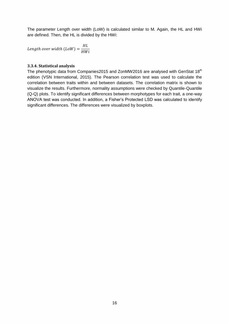
Head Length (HL), Head Width (HWi) and Head

Weight (HWe) are straight forward traits which

represent the length, width and weight of the

cabbage head. Furthermore, Core Length (CL)

represents the maximum length of the core or pith in

the cabbage head (figure 11). Due to time

limitations, Head Volume (HV) and Head Density

(HD) were not analysed by picture analysis.

The qualitative trait Head Shape was subdivided in

six quantitative parameters (appendix 1.3). The

parameter Roundness (R) is calculated by

subtracting the standard deviation over the distance

of radii from one:

𝑅𝑜𝑢𝑛𝑑𝑛𝑒𝑠𝑠 (𝑅) = 1 −𝑆𝑖𝑔𝑚𝑎

𝐷𝑖𝑠𝑡𝑎𝑛𝑐𝑒

For the parameter AreaRatio (AR), the cabbage is

divided into two halves. The width of the cabbage is measured from top to bottom for the

upper half and lower half. This has resulted in a plot of which the area was calculated for the

upper and lower half. The area under the graph of the upper half was called S1 and the area

under the lower half was called S2. The AR was calculated by:

𝐴𝑟𝑒𝑎𝑅𝑎𝑡𝑖𝑜 (𝐴𝑅) =𝑆1

𝑆2

The parameter Phi (P) holds the orientation of a fitted ellipse on the cabbage. An x-axis is

drawn over the image, then an ellipse is fitted to the cabbage head. Two radii are drawn: one

radius in y-axis direction (Ra) and one radius in x-axis direction (Rb). The angle between Ra

and the x-axis over the image defines P. Furthermore, Anisometry (A) is defined by:

𝐴𝑛𝑖𝑠𝑜𝑚𝑒𝑡𝑟𝑦 (𝐴) =𝑅𝑎

𝑅𝑏

The parameter Maxwidth row over half length (M) is calculated by defining the HL and HWi of

the cabbage head. Subsequently, the position of HWi (counted from top to bottom) is divided

by half HL.

𝑀𝑎𝑥𝑤𝑖𝑑𝑡ℎ 𝑟𝑜𝑤 𝑜𝑣𝑒𝑟 ℎ𝑎𝑙𝑓 𝑙𝑒𝑛𝑔𝑡ℎ (𝑀) =𝑝𝑜𝑠𝑖𝑡𝑖𝑜𝑛 𝐻𝑊𝑖

12 𝐻𝐿

HL

CL

HWi

Figure 11: White cabbage head with Head Length, Head Width and Core Length.

16

The parameter Length over width (LoW) is calculated similar to M. Again, the HL and HWi

are defined. Then, the HL is divided by the HWi:

𝐿𝑒𝑛𝑔𝑡ℎ 𝑜𝑣𝑒𝑟 𝑤𝑖𝑑𝑡ℎ (𝐿𝑜𝑊) =𝐻𝐿

𝐻𝑊𝑖

3.3.4. Statistical analysis

The phenotypic data from Companies2015 and ZonMW2016 are analysed with GenStat 18th

edition (VSN International, 2015). The Pearson correlation test was used to calculate the

correlation between traits within and between datasets. The correlation matrix is shown to

visualize the results. Furthermore, normality assumptions were checked by Quantile-Quantile

(Q-Q) plots. To identify significant differences between morphotypes for each trait, a one-way

ANOVA test was conducted. In addition, a Fisher’s Protected LSD was calculated to identify

significant differences. The differences were visualized by boxplots.

17

4. Results First, phenotypic data from Companies2015 and ZonMW2016 will be presented (paragraph

4.1). In paragraph 4.2, the population structure is treated and the results of the GWAS is

described in paragraph 4.3. Finally, some candidate genes for a subset of the marker trait

associations will be presented.

4.1. Phenotypic data Phenotypic data from two datasets will be presented in this section. The third dataset,

WURField2015 was already analysied previous year by Slob, 2016. Correlations between

traits within datasets are shown and the variance between morphotypes is tested with a one-

way ANOVA followed by a Fisher’s protected LSD for each trait. Significant differences of

traits between different cabbage types (white, red, savoy and pointed) are presented.

4.1.1. Companies2015

In the Companies2015 dataset, 121 heading cabbage accessions were phenotyped

belonging to four morphotypes. However, not all eight traits were scored for all cabbage

types. Only 46 accessions contained data for all traits. Based on these accessions, a

Pearson correlation matrix was calculated. Head Weight and Head Width have a positive

correlation (r =0.64). Other correlations involving Blistering, Head Density, Head Length,

Core Length, Stem Length and Uniformity were not found in this dataset (appendix 6.1).

Normality assumptions were checked for the eight traits that were scored. The distribution

was analysed by Q-Q plots with a 95% confidence interval (appendix 6.2). As can be seen,

Blistering, Head Density and Uniformity were scored in a qualitative manner which does not

lead to normally distributed data. Significant differences were found between cabbage types

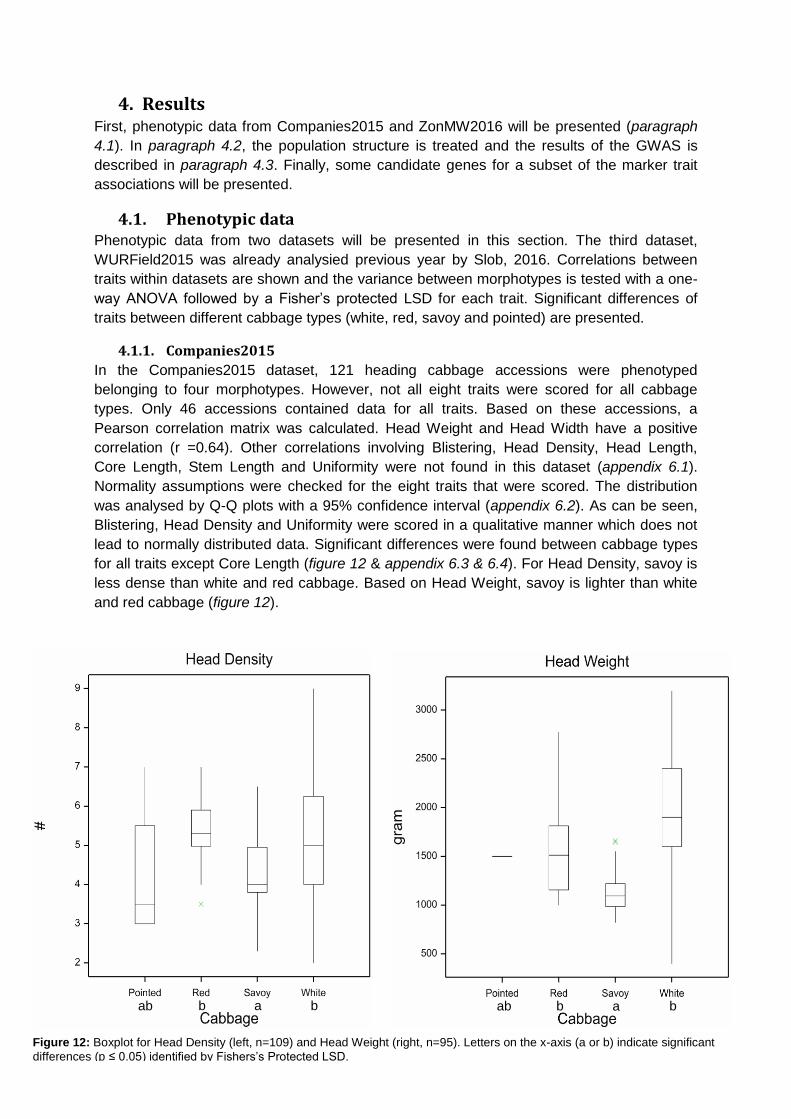
for all traits except Core Length (figure 12 & appendix 6.3 & 6.4). For Head Density, savoy is

less dense than white and red cabbage. Based on Head Weight, savoy is lighter than white

and red cabbage (figure 12).

ab b a b ab b a b

Figure 12: Boxplot for Head Density (left, n=109) and Head Weight (right, n=95). Letters on the x-axis (a or b) indicate significant

differences (p ≤ 0.05) identified by Fishers’s Protected LSD.

18

Leaf blistering is a typical savoy cabbage trait that was not measured in red cabbage.

However, it was measured in white and pointed cabbage. Unsurprisingly, savoy has more

severe blistering than white and pointed cabbage. Core Length showed no significant

differences between cabbage types. For Head Length, pointed is significantly longer than

red, savoy and white cabbage. Additionally, white cabbages are on average broader than

pointed, red and savoy cabbages for Head Width. Red cabbage is more uniform than white

and savoy cabbage (appendix 6.3 & 6.4).

4.1.2. ZonMW 3D Digileaf

In the ZonMW2016 dataset, 111 heading cabbage accessions were present. A block effect

was identified for HL and LoW (appendix 5.3 & 5.4). Therefore, HL and LoW from block A

and B were treated as separate traits in the analysis. In the dataset, ten traits were measured

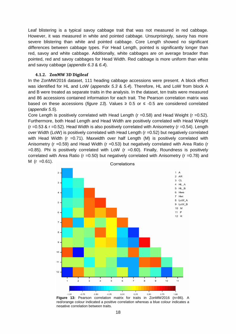
and 86 accessions contained information for each trait. The Pearson correlation matrix was

based on these accessions (figure 13). Values ≥ 0.5 or ≤ -0.5 are considered correlated

(appendix 5.5).

Core Length is positively correlated with Head Length (r =0.58) and Head Weight (r =0.52).

Furthermore, both Head Length and Head Width are positively correlated with Head Weight

(r =0.53 & r =0.52). Head Width is also positively correlated with Anisometry (r =0.54). Length

over Width (LoW) is positively correlated with Head Length (r =0.52) but negatively correlated

with Head Width (r =0.71). Maxwidth over half Length (M) is positively correlated with

Anisometry (r =0.59) and Head Width (r =0.53) but negatively correlated with Area Ratio (r

=0.85). Phi is positively correlated with LoW (r =0.60). Finally, Roundness is positively

correlated with Area Ratio (r =0.50) but negatively correlated with Anisometry (r =0.78) and

M (r =0.61).

Figure 13: Pearson correlation matrix for traits in ZonMW2016 (n=86). A

red/orange colour indicated a positive correlation whereas a blue colour indicates a negative correlation between traits.

19

Normality assumptions were violated for Anisometry, Phi and Roundness (appendix 5.6).

Head Length, Head Width, Head Weight, Core Length, Length over Width, AreaRatio and

Maxwidth over half Length are around normal distributed in the Q-Q plot. Significant

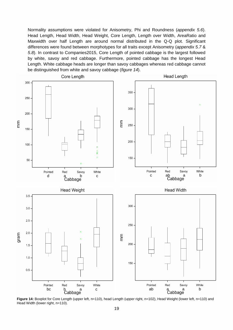
differences were found between morphotypes for all traits except Anisometry (appendix 5.7 &

5.8). In contrast to Companies2015, Core Length of pointed cabbage is the largest followed

by white, savoy and red cabbage. Furthermore, pointed cabbage has the longest Head

Length. White cabbage heads are longer than savoy cabbages whereas red cabbage cannot

be distinguished from white and savoy cabbage (figure 14).

d c b a c b a ab

bc c a b ab b a a

Figure 14: Boxplot for Core Length (upper left, n=110), head Length (upper right, n=102), Head Weight (lower left, n=110) and

Head Width (lower right, n=110).

20

White cabbage has the highest Head Weight. Pointed does not differ from red or savoy but

red is heavier than savoy cabbage. White cabbage has a higher Head Width than red and

savoy cabbage (figure 14).

Anisometry does not have significant differences between cabbage types. Pointed cabbage

has a lower AreaRatio than red, savoy and white cabbage. Length over Width of white and

savoy cabbages is lower than red and pointed cabbage. Maxwidth over half Length of red

and white cabbages is lower than savoy and pointed cabbages. Phi of white cabbage is

lower than red and pointed cabbage whereas pointed is higher than savoy and white

cabbage. Roundness of pointed cabbage is lower than savoy and white cabbage and

Roundness of white cabbage is higher than red and pointed cabbage (appendix 5.7 & 5.8).

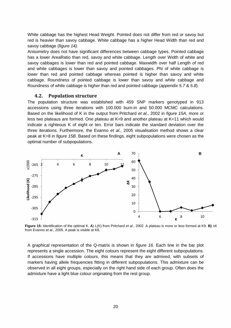
4.2. Population structure The population structure was established with 459 SNP markers genotyped in 913

accessions using three iterations with 100.000 burn-in and 50.000 MCMC calculations.

Based on the likelihood of K in the output from Pritchard et al., 2002 in figure 15A, more or

less two plateaus are formed. One plateau at K=9 and another plateau at K=11 which would

indicate a righteous K of eight or ten. Error bars indicate the standard deviation over the

three iterations. Furthermore, the Evanno et al., 2005 visualisation method shows a clear

peak at K=8 in figure 15B. Based on these findings, eight subpopulations were chosen as the

optimal number of subpopulations.

A graphical representation of the Q-matrix is shown in figure 16. Each line in the bar plot

represents a single accession. The eight colours represent the eight different subpopulations.

If accessions have multiple colours, this means that they are admixed, with subsets of

markers having allele frequencies fitting in different subpopulations. This admixture can be

observed in all eight groups, especially on the right hand side of each group. Often does the

admixture have a light blue colour originating from the rest group.

0

10

20

30

40

50

60

70

4 6 8 10

∆K

K -315

-305

-295

-285

-275

-265 2 4 6 8 10 12

Like

liho

od

(K

) x1

00

0

K

Figure 15: Identification of the optimal K. A) L(K) from Pritchard et al., 2002. A plateau is more or less formed at K9. B) ∆K from Evanno et al., 2005. A peak is visible at K8.

A B

21

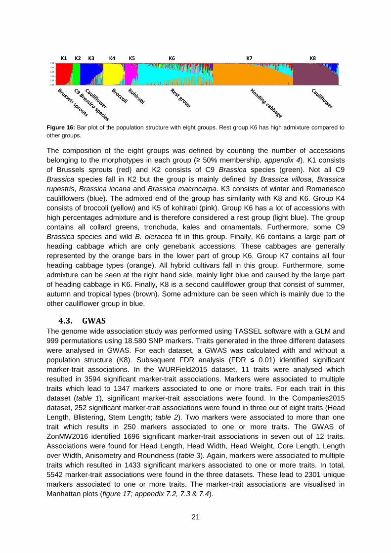
Figure 16: Bar plot of the population structure with eight groups. Rest group K6 has high admixture compared to

other groups.

The composition of the eight groups was defined by counting the number of accessions

belonging to the morphotypes in each group (≥ 50% membership, appendix 4). K1 consists

of Brussels sprouts (red) and K2 consists of C9 Brassica species (green). Not all C9

Brassica species fall in K2 but the group is mainly defined by Brassica villosa, Brassica

rupestris, Brassica incana and Brassica macrocarpa. K3 consists of winter and Romanesco

cauliflowers (blue). The admixed end of the group has similarity with K8 and K6. Group K4

consists of broccoli (yellow) and K5 of kohlrabi (pink). Group K6 has a lot of accessions with

high percentages admixture and is therefore considered a rest group (light blue). The group

contains all collard greens, tronchuda, kales and ornamentals. Furthermore, some C9

Brassica species and wild B. oleracea fit in this group. Finally, K6 contains a large part of

heading cabbage which are only genebank accessions. These cabbages are generally

represented by the orange bars in the lower part of group K6. Group K7 contains all four

heading cabbage types (orange). All hybrid cultivars fall in this group. Furthermore, some

admixture can be seen at the right hand side, mainly light blue and caused by the large part

of heading cabbage in K6. Finally, K8 is a second cauliflower group that consist of summer,

autumn and tropical types (brown). Some admixture can be seen which is mainly due to the

other cauliflower group in blue.

4.3. GWAS The genome wide association study was performed using TASSEL software with a GLM and

999 permutations using 18.580 SNP markers. Traits generated in the three different datasets

were analysed in GWAS. For each dataset, a GWAS was calculated with and without a

population structure (K8). Subsequent FDR analysis (FDR ≤ 0.01) identified significant

marker-trait associations. In the WURField2015 dataset, 11 traits were analysed which

resulted in 3594 significant marker-trait associations. Markers were associated to multiple

traits which lead to 1347 markers associated to one or more traits. For each trait in this

dataset (table 1), significant marker-trait associations were found. In the Companies2015

dataset, 252 significant marker-trait associations were found in three out of eight traits (Head

Length, Blistering, Stem Length; table 2). Two markers were associated to more than one

trait which results in 250 markers associated to one or more traits. The GWAS of

ZonMW2016 identified 1696 significant marker-trait associations in seven out of 12 traits.

Associations were found for Head Length, Head Width, Head Weight, Core Length, Length

over Width, Anisometry and Roundness (table 3). Again, markers were associated to multiple

traits which resulted in 1433 significant markers associated to one or more traits. In total,

5542 marker-trait associations were found in the three datasets. These lead to 2301 unique

markers associated to one or more traits. The marker-trait associations are visualised in

Manhattan plots (figure 17; appendix 7.2, 7.3 & 7.4).

22

WURField2015 – No PS

WURField2015 – K8

Companies – No PS

Companies2015 – K8

ZonMW2016 – No PS

ZonMW2016 – K8

Companies – No PS

Companies2015 – K8

WURField2015 – No PS

WURField2015 – K8

ZonMW2016 – No PS

ZonMW2016 – K8

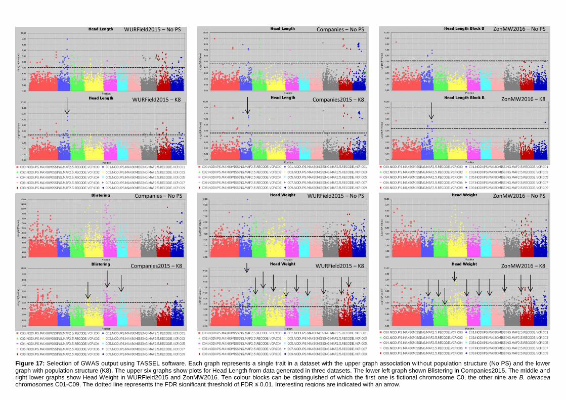
Figure 17: Selection of GWAS output using TASSEL software. Each graph represents a single trait in a dataset with the upper graph association without population structure (No PS) and the lower

graph with population structure (K8). The upper six graphs show plots for Head Length from data generated in three datasets. The lower left graph shown Blistering in Companies2015. The middle and right lower graphs show Head Weight in WURField2015 and ZonMW2016. Ten colour blocks can be distinguished of which the first one is fictional chromosome C0, the other nine are B. oleracea chromosomes C01-C09. The dotted line represents the FDR significant threshold of FDR ≤ 0.01. Interesting regions are indicated with an arrow.

23

To identify interesting regions in terms of marker trait associations, certain assumptions have

been made. When many significant markers were found, for example for Head Weight in

WURField2015 and ZonMW2016, emphasis was laid on markers that form a peak.

Furthermore, a peak is considered interesting if the LOD score is increased in the analysis

with population structure correction compared to no population structure correction. When a

limited number of significant associations was found, the emphasis was on single markers

that increased in LOD score when analysed with population structure correction compared to

analysis without population structure correction. When markers from the same genomic

region are associated with a trait phenotyped in different datasets, the region is considered a

candidate region.

Candidate regions associated with traits were identified from the Manhattan plots in figure 17

and are indicated with an arrow. A limited number of markers are significantly associated

with the trait Head Length in all three datasets (upper three graphs). Therefore, single

markers are also considered interesting when they occur in multiple datasets and increase in

LOD score after population structure correction. The region on C01 (arrow at blue dots) is

considered a candidate region, as markers form a peak in both WURField2015 and

Companies2015 datasets and in the Companies2015 dataset the LOD score of the

associated markers increased from 7.1 without population structure to 7.6 with population

structure. This region is selected as candidate region for HL. Blistering in the lower left graph

was only measured in Companies 2015 making comparison across datasets impossible.

After population structure correction, 130 markers were significantly associated with

Blistering. Candidate regions in the form of peaks appear on C03 (yellow), C04 (pink) and

C05 (light blue). No significant marker-trait associations were identified for Head Weight in

Companies2015. However, many significant marker-trait associations for HWe were found in

WURField2015 (569) and ZonMW2016 (291), even after population structure correction.

Therefore, peaks were chosen that occur in WURField2015 and ZonMW2016 and increase

in LOD score after population structure correction. In total, 14 peak markers were chosen as

indicators of candidate regions (table 4).

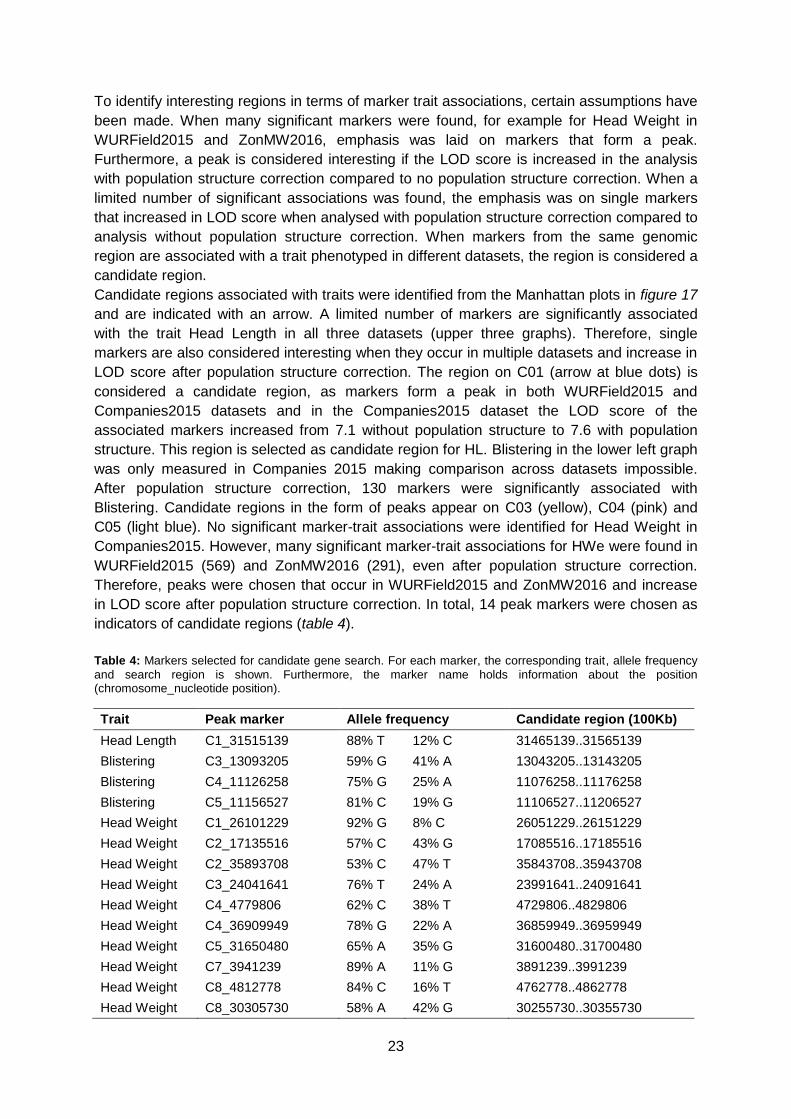
Table 4: Markers selected for candidate gene search. For each marker, the corresponding trait, allele frequency

and search region is shown. Furthermore, the marker name holds information about the position (chromosome_nucleotide position).

Trait Peak marker Allele frequency Candidate region (100Kb)

Head Length C1_31515139 88% T 12% C 31465139..31565139

Blistering C3_13093205 59% G 41% A 13043205..13143205

Blistering C4_11126258 75% G 25% A 11076258..11176258

Blistering C5_11156527 81% C 19% G 11106527..11206527

Head Weight C1_26101229 92% G 8% C 26051229..26151229

Head Weight C2_17135516 57% C 43% G 17085516..17185516

Head Weight C2_35893708 53% C 47% T 35843708..35943708

Head Weight C3_24041641 76% T 24% A 23991641..24091641

Head Weight C4_4779806 62% C 38% T 4729806..4829806

Head Weight C4_36909949 78% G 22% A 36859949..36959949

Head Weight C5_31650480 65% A 35% G 31600480..31700480

Head Weight C7_3941239 89% A 11% G 3891239..3991239

Head Weight C8_4812778 84% C 16% T 4762778..4862778

Head Weight C8_30305730 58% A 42% G 30255730..30355730

24

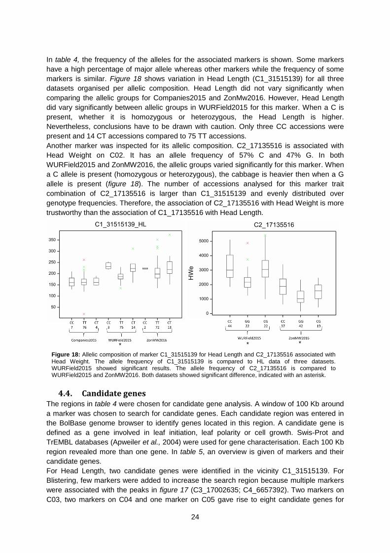
In table 4, the frequency of the alleles for the associated markers is shown. Some markers

have a high percentage of major allele whereas other markers while the frequency of some

markers is similar. Figure 18 shows variation in Head Length (C1_31515139) for all three

datasets organised per allelic composition. Head Length did not vary significantly when

comparing the allelic groups for Companies2015 and ZonMw2016. However, Head Length

did vary significantly between allelic groups in WURField2015 for this marker. When a C is

present, whether it is homozygous or heterozygous, the Head Length is higher.

Nevertheless, conclusions have to be drawn with caution. Only three CC accessions were

present and 14 CT accessions compared to 75 TT accessions.

Another marker was inspected for its allelic composition. C2_17135516 is associated with

Head Weight on C02. It has an allele frequency of 57% C and 47% G. In both

WURField2015 and ZonMW2016, the allelic groups varied significantly for this marker. When

a C allele is present (homozygous or heterozygous), the cabbage is heavier then when a G

allele is present (figure 18). The number of accessions analysed for this marker trait

combination of C2_17135516 is larger than C1_31515139 and evenly distributed over

genotype frequencies. Therefore, the association of C2_17135516 with Head Weight is more

trustworthy than the association of C1_17135516 with Head Length.

4.4. Candidate genes The regions in table 4 were chosen for candidate gene analysis. A window of 100 Kb around

a marker was chosen to search for candidate genes. Each candidate region was entered in

the BolBase genome browser to identify genes located in this region. A candidate gene is

defined as a gene involved in leaf initiation, leaf polarity or cell growth. Swis-Prot and

TrEMBL databases (Apweiler et al., 2004) were used for gene characterisation. Each 100 Kb

region revealed more than one gene. In table 5, an overview is given of markers and their

candidate genes.

For Head Length, two candidate genes were identified in the vicinity C1_31515139. For

Blistering, few markers were added to increase the search region because multiple markers

were associated with the peaks in figure 17 (C3_17002635; C4_6657392). Two markers on

C03, two markers on C04 and one marker on C05 gave rise to eight candidate genes for

Figure 18: Allelic composition of marker C1_31515139 for Head Length and C2_17135516 associated with

Head Weight. The allele frequency of C1_31515139 is compared to HL data of three datasets. WURField2015 showed significant results. The allele frequency of C2_17135516 is compared to WURField2015 and ZonMW2016. Both datasets showed significant difference, indicated with an asterisk.

* * *

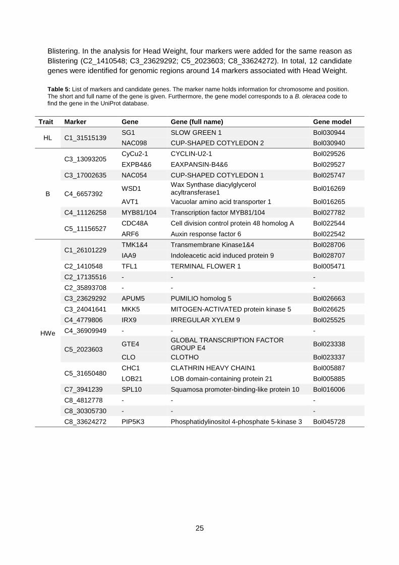
25

Blistering. In the analysis for Head Weight, four markers were added for the same reason as

Blistering (C2_1410548; C3_23629292; C5_2023603; C8_33624272). In total, 12 candidate

genes were identified for genomic regions around 14 markers associated with Head Weight.

Table 5: List of markers and candidate genes. The marker name holds information for chromosome and position.

The short and full name of the gene is given. Furthermore, the gene model corresponds to a B. oleracea code to find the gene in the UniProt database.

Trait Marker Gene Gene (full name) Gene model

HL C1_31515139 SG1 SLOW GREEN 1 Bol030944

NAC098 CUP-SHAPED COTYLEDON 2 Bol030940

B

C3_13093205 CyCu2-1 CYCLIN-U2-1 Bol029526

EXPB4&6 EAXPANSIN-B4&6 Bol029527

C3_17002635 NAC054 CUP-SHAPED COTYLEDON 1 Bol025747

C4_6657392 WSD1

Wax Synthase diacylglycerol acyltransferase1

Bol016269

AVT1 Vacuolar amino acid transporter 1 Bol016265

C4_11126258 MYB81/104 Transcription factor MYB81/104 Bol027782

C5_11156527 CDC48A Cell division control protein 48 homolog A Bol022544

ARF6 Auxin response factor 6 Bol022542

HWe

C1_26101229 TMK1&4 Transmembrane Kinase1&4 Bol028706

IAA9 Indoleacetic acid induced protein 9 Bol028707

C2_1410548 TFL1 TERMINAL FLOWER 1 Bol005471

C2_17135516 - - -

C2_35893708 - - -

C3_23629292 APUM5 PUMILIO homolog 5 Bol026663

C3_24041641 MKK5 MITOGEN-ACTIVATED protein kinase 5 Bol026625

C4_4779806 IRX9 IRREGULAR XYLEM 9 Bol025525

C4_36909949 - - -

C5_2023603 GTE4

GLOBAL TRANSCRIPTION FACTOR GROUP E4

Bol023338

CLO CLOTHO Bol023337

C5_31650480 CHC1 CLATHRIN HEAVY CHAIN1 Bol005887

LOB21 LOB domain-containing protein 21 Bol005885

C7_3941239 SPL10 Squamosa promoter-binding-like protein 10 Bol016006

C8_4812778 - - -

C8_30305730 - - -

C8_33624272 PIP5K3 Phosphatidylinositol 4-phosphate 5-kinase 3 Bol045728

26

5. Discussion

5.1. Phenotypic data First, the quality of phenotypic data will be discussed. Subsequently, the correlation between

traits within and between datasets will be discussed. Finally, traits that show significant

differences between morphotypes will be discussed. The datasets in this research

(WURField2015, Companies2015 and ZonMW2016) are independent from one another. The

phenotypic data was gathered at different locations and different years. Furthermore, a

collection of different accessions was used with a limited number of overlapping accessions

(figure 10).

5.1.1. Data quality

The WURField2015 dataset contained a total of 160 accessions of which 140 were modern

hybrids and 20 were genebank accessions. A variety of traits were measured by image

analysis software ImageJ. Overall, the measurements give a good approximation of the trait

values. However, traits such as Head Density, Head Roundness, Head Shape and Head

Volume will be measured more accurately with 3D imaging software compared to

measurements taken from 2D pictures.

The goal of the ZonMW dataset was to identify and quantify heading parameters using a 3D

camera set up. Furthermore, advanced imaging software such as Halcon would be used for

the 3D picture analysis. In total 111 accessions were phenotyped of which 65 were modern

hybrids and 46 were genebank accessions. The cabbage heads were harvested by cutting

them just beneath the attachment of the outer leaves of the cabbage head. Loose leaves that

did not wrap around the cabbage head were removed before images were taken. Within the

111 accessions, sub-morphotypes were identified. Most of the accession have a known

phenotype, white, red, savoy or pointed cabbage. However, the phenotype of some

accessions was still unknown. These accessions could be sown on the field next year to

phenotype them correctly. This extra phenotypic information could be incorporated into the

analysis. The traits Head Weight, Head Length and Head Width were correctly measured. A

correct measurement is a measurement that was performed by an algorithm and gives the

same output as a measurement by hand.

Core Length was not correctly measured by the algorithm especially in white and pointed

cabbage types. This is due to the inner colour of the cabbage. White, pointed and savoy

cabbage have a white core and white/green leaves whereas red cabbage has a white core

and purple leaves. An adjustment in the algorithm has to be made to be able to discriminate

between core and leaf colour. Halcon is able to separate the images in multiple colour

spectra. When the yellow colour spectrum is filtered out, differences in core and leaves can

be seen. Core Length is an interesting trait for breeders because a good hybrid has a small

core which leads to a larger edible part of the cabbage. Furthermore, it is expected that a

smaller Core Length increases the density of the cabbage head, which is also favoured by

breeders and consumers. However, the relationship between Core Length and Head Density

is unknown because Core Length was not correctly measured and Head Density still has to

be measured by the computer vision and robotics group. Because Core Length is important

for breeding purposes and selection on the trait must have happened, it would be interesting

to identify candidate gens that are involved in defining the Core Length.

The trait Head Shape was divided into six parameters, ranging from an ellipse shape to

pointed phenotypes (appendix 2). The idea was that these six parameters would be used by

an algorithm to define the Head Shape. Later in the project, the decision was made that

27

quantitative parameters would be better for association analysis than the qualitative trait

Head Shape. Phi is not informative as trait parameter but is used by the algorithm to

establish the orientation of the cabbage on the image and is used by the software to make a

decision if the picture should be turned 90 degrees or not before other parameters could be

calculated. The other shape parameters, Anisometry, AreaRatio, Length_over_Width,

Roundness and Maxwidth_row_over_half_Length, give information about the heading

cabbage shape.

Due to circumstances in the computer vision and robotics department, Head Density and

Head Volume were not measured in the analysis. Head Density is a measure for the density

or compactness of the cabbage head. This is an interesting trait to study because large

variation in the cabbage density is observed. Furthermore, this is an important trait for

breeding companies and selection must have happened on this trait. It would be interesting

to identify genes that make a difference in a loose or dense cabbage structure. If Head

Density is still not measured in future research, an approximation for density can be used.

Based on Head Density from the WURField2015 dataset. The Head Weight can be divided

by the Head Volume to give an indication for Head Density. Head Volume is an interesting

trait because it gives an indication about cabbage size and can be used in parameter

calculation described above. One would expect it to be positively correlated with Head

Length, Head Width, Core Length and Head Weight. Indeed, in the WURField2015 dataset a

positive correlation was found for Head Volume with Head Length, Head Width and Head

Weight. Moreover, Head Density is negatively correlated with Head Length and Head Width

in WURField2015. This implies that a denser cabbage is shorter and less broad; i.e. smaller.

Based on these hypotheses, it would be a good addition to the ZonMW2016 dataset if Head

Density and Head Volume were included based on 3D image analysis.

The Companies2015 dataset contains 121 genebank accessions. Heading types were

phenotyped at different breeding companies. This resulted in 26 measured traits of which 14

were real heading cabbage traits (appendix 1.2). However, the traits were not scored for

each cabbage type. Eight traits were chosen for analysis which were measured in at least

two cabbage types (table 2). The assumption was made that traits measured by different

companies can be compared with each other, on the condition that the same plant part was

compared. Head Weight, Head Length, Head Width and Core Length are quantitative traits

and are correctly measured. Stem Length was not measured consistently. The trait was not

scored in savoy cabbage and in red cabbage very high values were observed. This indicates

that different interpretations of Stem Length were applied. Blistering and Head Density were

also measured in a qualitative manner. Unfortunately, the cabbage heads were not

harvested at the same moment for all cabbage types. Furthermore, it is unknown if the

harvest date within a cabbage type was the same. This makes the quality of the measured

data hard to judge because it was carried out by other people than the writers of this thesis. It

is assumed that noise is introduced by the varying harvest dates and because

measurements were takes by different persons.

5.1.2. Correlations within and between datasets

In Companies2015, hardly any correlations between traits were found within the dataset. The

only correlation found was between HWe and HWi. When a cabbage is heavier, it is logical

that it is broader but it would also make sense that it would be longer or more dense.

However, this was not observed within this dataset. The absence of correlations between

traits can be due to the fact that Companies2015 contained only genebank accessions.

Genebank accessions are heterogeneous, and thus accessions are often not uniform in

28

appearance. This results in variation within accessions. However, 46 out of 121 accessions

were used in the Pearson correlation test because the Pearson correlation test requires

accessions that contain data for each trait. If more accessions contained data for all traits

there is a possibility that more correlations would be found. Another method to identify

correlations would be the use of subsets of traits. For example, Blistering was not measured

for red cabbage. Therefore, all red cabbages were omitted in the Pearson correlation test.

When Blistering is removed from the traits in the Pearson correlation test, more accessions

will be available to calculate the correlation between the remaining traits.

In ZonMW2016, more significant correlations were found. Head Weight is positively

correlated with Head Length, Head Width and Core Length. This makes sense because a

longer cabbage or broader cabbage is larger and thus heavier. Unsurprisingly Core Length is

positively correlated with Head Length because a longer head has a longer core. However,

we have to keep in mind that Core Length was not measured correctly in all cases. It would

be interesting to find out if the Core Length is still positively correlated to Head Length when

the algorithm can identify Core Length correctly or the Core Length is manually calculated.

The Head Shape parameters show correlations as well. Length_over_Width is negatively

correlated with Head Width and positively correlated with Head Length. This is logical since

Head Length is divided by Head Width. Head Width is positively correlated with Anisometry

and Maxwidth over half Length because Anisometry and Maxwidth over half Length both use

Head Width in their parameter calculation. Subsequently, Anisometry and Maxwidth over half

Length are positively correlated as well whereas Maxwidth over half Length and AreaRatio

are negatively correlated.

When we compare the relationships of ZonMW2016 and Companies2015 to WURField2015

the same conclusions can be drawn with regard to Head Weight, Head Length and Head

Width. The shape parameters of ZonMW2016 cannot be compared to Head Shape of

WURField2015.

5.1.3. Differences between morphotypes

Quantitative traits should be analysed with a parametric test and qualitative data should be

analysed with a non-parametric test. The comparison between parametric and non-

parametric data is hard. Therefore, all data was analysed with parametric tests. Normality

assumptions were violated in Companies2015 and ZonMW2016 by qualitative traits

(Blistering, Head Density, Uniformity) but also by quantitative traits (Anisometry, Phi,

Roundness, Stem Length) (appendix 5.6 & 6.2). However, this is not considered a problem

because the sample size of 121 and 111 should be large enough for the data to behave as

approximately normally distributed data (Central Limit Theorem (Whitlock & Schlutter, 2009)).

Significant differences were found between cabbage types by ANOVA analysis. In the

Companies2015 dataset (appendix 6.3 & 6.4), pointed cabbage was represented only once

in 121 accessions. Therefore, no conclusions can be drawn regarding this cabbage type.

Savoy cabbage has the lowest density and weight. This is logical because savoy is known

for its looser structure. Moreover, savoy cabbage has higher blistering than white cabbage.

This is also logical because savoy is known for the blistering structure of the leaves.

Blistering was not measured in red cabbage. No significant differences were found for Core

Length. This is remarkable because differences do exist. It may be explained by the absence

of pointed cabbage in the dataset because it has in theory the highest Head Length and thus

Core Length. Another explanation may be that the genebank accessions did not have had

strict selection on Core Length because this material has not extensively been used in

breeding. No significant differences were found in Head Length. This is also due to the

29

absence of pointed cabbage which has in theory the largest Head Length (appendix 2). A

high standard deviation in Head Length is observed for white cabbage. This is because there

is large variation in Head Length for white cabbages. Shape class one to five, which range

from transverse narrow elliptic to broad obovate, are observed within the white cabbages.

These different shape classes have a large impact on Head Length. Subsequently, this wide

variation in white cabbage can be observed for Head Width. White cabbage is significantly

broader than the other cabbage types. Uniformity is omitted in further analysis because this

trait was measured within accessions and not between accessions.

More significant differences between morphotypes were found in the ZonMW2016 dataset.

Results are shown in figure 14 and appendix 5.7 and 5.8. The Head Length of pointed

cabbage is significantly longer than that of the other cabbage types. This is in line with HL

expectations. Furthermore, Core Length of pointed cabbage is also longer than that of the

other cabbage types. This can be explained by the correlation between Head Length and

Core Length: the longer the cabbage, the longer the core. Pointed cabbage has a higher

Core Length which lead to a larger distance between subsequent leaves within the cabbage

head. This larger distance between leaves increase the total Head Length. Furthermore,

pointed cabbage is expected to wrap its leaves in a different manner than other cabbage

types which also adds to the Head Length. Unfortunately, the hypotheses between Head

Length and Core Length cannot be tested in the ZonMW2016 dataset. Core Length was not

measured correctly and is therefore omitted in further analysis. White cabbage has a higher

Head Width than red and savoy cabbage. This is due to shape class one and two,

representing transverse narrow- and transverse elliptic shape classes, which are observed in

white cabbages. Moreover, white cabbage has a higher weight than red and savoy cabbage.

A reason can be that white cabbage tends to be larger. Both longer and broader than red

and savoy cabbage. Another hypothesis can be that white cabbage has a higher density than

red and savoy cabbage. In order to test this hypothesis, Head Density should be measured

in an accurate manner. This can be done by the algorithm by quantifying Head Density. For

example, the looser the cabbage head, the more shadow is visible on the image. The

algorithm can quantify this degree of shading. Furthermore, a distinction can be made in

upper and lower density of the cabbage head. The lower part of the cabbage head, around

the Core Length, tends to be looser of structure than the upper part of the cabbage head.

No significant differences were found for Anisometry. An explanation may be the number of

outliers in the dataset which can be caused by the transverse narrow- and transverse elliptic

shapes of white cabbage. The algorithm could have switched Ra with Rb which lead to

outliers in the data. The Area Ratio for pointed cabbage is smaller than for the other cabbage

types. This is logical because the upper half of a pointed cabbage has a smaller area than

the lower half of the pointed cabbage. Since upper area is divided by lower area, the

AreaRatio will be < 0 whereas the upper and lower area of other cabbage types will be more

or less equal which leads to an AreaRatio of approximately 1. Length_over_Width of pointed

and red cabbage is larger than savoy and white cabbage. This is logical for pointed cabbage

since the Head Length is longer than Head Width (shape class six and seven). In addition, it

seems that red cabbage is always longer than broad. This is also logical because red

cabbage has shape class four and five wherein Head Length is longer than Head Width. The

shape classes one, two and three in white cabbage and two and three in savoy cabbage

cause the difference with pointed (broad/angular ovate) and red cabbage (broad obovate).

Maxwidth over half Length of red and white cabbage is smaller than pointed and savoy

cabbage. This makes sense because shape class five (broad obovate) is observed in white

and red cabbage. Broad obovate cabbage results in a smaller position number (counted from

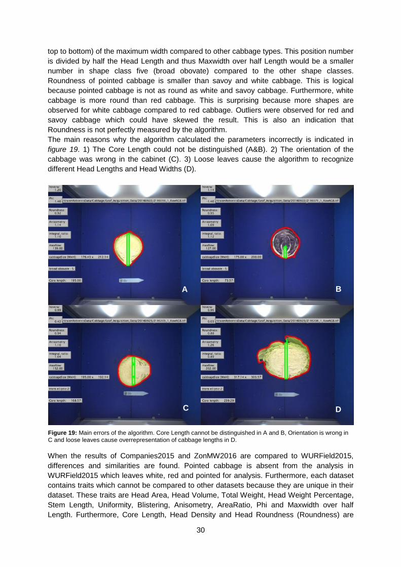
30

C

top to bottom) of the maximum width compared to other cabbage types. This position number

is divided by half the Head Length and thus Maxwidth over half Length would be a smaller

number in shape class five (broad obovate) compared to the other shape classes.

Roundness of pointed cabbage is smaller than savoy and white cabbage. This is logical

because pointed cabbage is not as round as white and savoy cabbage. Furthermore, white

cabbage is more round than red cabbage. This is surprising because more shapes are

observed for white cabbage compared to red cabbage. Outliers were observed for red and

savoy cabbage which could have skewed the result. This is also an indication that

Roundness is not perfectly measured by the algorithm.

The main reasons why the algorithm calculated the parameters incorrectly is indicated in

figure 19. 1) The Core Length could not be distinguished (A&B). 2) The orientation of the

cabbage was wrong in the cabinet (C). 3) Loose leaves cause the algorithm to recognize

different Head Lengths and Head Widths (D).

When the results of Companies2015 and ZonMW2016 are compared to WURField2015,

differences and similarities are found. Pointed cabbage is absent from the analysis in

WURField2015 which leaves white, red and pointed for analysis. Furthermore, each dataset

contains traits which cannot be compared to other datasets because they are unique in their

dataset. These traits are Head Area, Head Volume, Total Weight, Head Weight Percentage,

Stem Length, Uniformity, Blistering, Anisometry, AreaRatio, Phi and Maxwidth over half

Length. Furthermore, Core Length, Head Density and Head Roundness (Roundness) are

D

A B

A

C

A

Figure 19: Main errors of the algorithm. Core Length cannot be distinguished in A and B, Orientation is wrong in

C and loose leaves cause overrepresentation of cabbage lengths in D.

31

measured in a different way across datasets which also makes comparison hard. In other

words, Head Length, Head Width, Head Weight and Length_over_Width (Head Index) can

be compared across datasets. No large differences in Head Length, Head Width, Head

Weight and Length_over_Width were found across datasets.

A large improvement of the ZonMW2016 dataset was the controlled environment in where

the images were taken, compared to the images taken of the field in WURField2015.

Furthermore, the throughput was increased in ZonMW2016 by the use of an algorithm in

Halcon compared to semi-automated measurements in ImageJ in WURField2015. However,

al lot of work still has to be done for further analysis. For starters, leaf data still has to be

analysed. Leaf parameters have to be defined in cooperation with the computer vision and

robotics department. When the leaf traits have been measured, a GWAS can be conducted

on this data and compared to the results of WURField2015 GWAS output. Besides leaves,

the computer vision and robotics department still has to analyse Head Density and Head

Volume. These traits are considered important in breeding and need further research to

genetically understand cabbage density and volume. The algorithm, as it is now, is not able

to measure all traits correctly in ZonMW2016. Colours have to be split in different channels to

discriminate the Core Length from leaves. In future heading cabbage measurement, it is

suggested that the imaging is performed on both halves of the cabbage head that was

photographed from the cross-section side. This way you will get a good indication of Head

Volume because both halves of the cabbage are photographed instead of two times the

same half. Additionally, when the cabbage was not perfectly sliced in half, an average can be

taken. This approach needs a correction for depth in the image. Thicker cabbages are closer

to the camera resulting in an overestimation for cabbage size.

5.2. Genotypic data In this paragraph, the genotyping will be reviewed followed up by the population structure.

Finally, the GWAS and candidate genes will be discussed.

5.2.1. Genotyping

The accessions in the dataset were genotyped by SBG, a Keygene technology. One of the

restriction enzymes used, PstI, is methylation sensitive. This excludes sequence information

around methylated PstI sites which likely occur around the centromere. The dataset was

filtered with a genotype call of 80% which implies that each marker should be scored in at

least 80% of the accessions. Furthermore, a MAF of 2.5% was chosen. This means that

markers with a minor allele frequency lower or equal than 2.5% will be filtered out.

Accessions with more than 60% missing marker values were removed from the dataset

because these accessions were not considered informative enough for analysis. The MAF

filtering step proved to filter most markers out; from 85.168 to 18.580 markers. Minor alleles

can be important in for example finding resistance genes. The resistance genes are

expected to occur in low frequencies. To identify these genes, the low frequency markers are

especially interesting. However, low frequency markers also tend to be mistakes in the

genotypic data, possibly induced by the use of restriction enzymes or by sequencing errors.

This research aims to identify heading cabbage traits. The alleles involved in defining leaf

morphology are not expected to occur in low allele frequencies. Besides, running a GWAS

on 85.168 markers takes longer computational time. A dataset with 18.580 markers is easier

to work with but it is expected that marker-trait associations will be missed in the analysis.

This is due to a limited amount of markers in a region where the LD is low. The half

maximum LD decay in B. oleracea was estimated at 36.8 Kb by Cheng et al., 2016.

32

Furthermore, the reference genome is approximately 500 Mb. Based on these numbers, an

indication for a sufficient marker density can be given.

500 𝑀𝑏

36.8 𝐾𝑏= ~13.600 𝑚𝑎𝑟𝑘𝑒𝑟𝑠

The marker density would be sufficient with more than 13.600 markers evenly distributed

over the genome. In this research, 18.580 markers were used which is in theory enough.

However, the markers are not evenly distributed over the genome (appendix 7.5). Especially

the upper parts of C07, C09 and C02 as well as the lower part of C02 have a low amount of

markers. Further LD analysis is necessary as the LD varies over the genome; some regions

have had more recombination that other regions, for example low recombination frequencies

at centromeres and telomeres. Therefore, it is recommended that the LD will be calculated

over the genome from which haplotypes can be defined. Subsequently, the haplotypes can

serve as input for the association analysis rather than SNPs. Haplotypes will be more

informative because multiple SNPs can be in LD with each other and define together a

haplotype (Brown & Weir, 2010; Gattepaill & Leslie, 2011). The LD analysis was not carried

out in this research due to limited time.

Filtering plays an important role in the organisation of genotypic data. In this research,

genetic information from 11 morphotypes was used to call SNPs. One would expect many

differences between morphotypes but Del Carpio et al., 2011 showed that the diversity within

a morphotype is larger than between morphotypes. This is due to the fact that in history,

most crosses were made within a morphotype and not between morphotypes and likely

means that only a small part of the genome is involved in morphotype specific traits. It would

be interesting to call SNPs solely based on the morphotypes of heading cabbage. One would

expect that in case all called SNPs are informative, the quality of the population structure will

improve and the quality of the association analysis might increase. If SNPs are called based

on heading cabbage, it is likely that the genetic information that discriminates a cabbage

from other morphotypes will be lost. However, these associations are lost when correcting by

population structure as well.

5.2.2. Population structure

For the population structure, 1376 SNP markers were selected which were evenly distributed

over the genome with a minimum distance of 250 Kb. Not all 1376 SNP markers were used

to build a population structure. The markers were thinned to 459 SNP markers to shorten

computational time. In the first run, a burn-in period of 50.000, MCMC calculations of 50.000

and three iterations were chosen as settings. However, the obtained results were not

consistent over the three runs. Therefore, the burn-in period was increased to 100.000. The

error bars in the Pritchard output in figure 15 indicate that there is still some deviation

between runs. Due to time limitations, this STRUCTURE output was chosen as population

structure.

Based on the Pritchard output, two plateaus can be identified at K=9 and K=11. This

indicates a righteous K of eight and ten. Since the interpretation of the Pritchard graph is

hard, Evanno et al., 2005 developed a method to visualize the STRUCTURE output. The

Evanno method is built from the Pritchard output. The first derivative (L’(K)) is obtained by

calculating the rate of change of L(K). From this L’(K) the second derivative (L’’(K)) is

obtained by calculating the rate of change in L’(K). The second derivative can be negative

and is therefore calculated as absolute values (|L’’(K)|). Finally, |L’’(K)| is divided by the

33

standard error of the Pritchard output. A peak in this graph indicates the righteous K.

However, the Evanno method is also not straight forward. Small K’s always have very high

values in the Evanno graph (figure 15). K=2 and K=3 are already removed from the graph to

clarify the peak at K8. These high values are due to a large rate of change in L(K) with lower

K’s. Therefore, the assumption was made that the Evanno graph should first become close

to zero before a subsequent peak was chosen as righteous K. Based on the Pritchard

manual, the K closest to zero should be chosen as righteous K. Accordingly, eight groups

were chosen as population structure.

When the Q matrix of K8 is researched, some accessions were fit into multiple groups based

on membership percentages. To make a clear group definition, accessions with a

membership of 50% or more were considered in the description. The formed groups are

logical and are shown in figure 16 and appendix 4. Surprisingly, cauliflowers are represented

by two groups: K3 for winter and Romanesco types and K8 for summer, autumn and tropical

types. Furthermore, heading cabbage has their own group including all hybrids and some

genebank material. A large proportion of heading cabbage accessions is present in rest

group K6 indicated by the orange colour of heading cabbage group K7. These heading

cabbages represent all genebank material and thus these accessions are more likely to be

assigned to the rest group than hybrids. The germplasm of hybrids nowadays will be used

more often than genebank material in breeding, thus is more related and groups together but

has lost a lot of variation. Accordingly, the genebank accessions are an important source of

genetic variation. Group K2 is a group that contains Brassica species with nine

chromosomes. Remarkably, not all C9 Brassica species group into K2 but also a large

proportion is assigned to rest group K6. B. villosa and B. rupestris are solely assigned to K2

whereas the majority of B. incana and B. macrocarpa are assigned to K2 and the remaining

species (B. bourgeaui, B. cretica, B. insularis, B. maurorum and B. montana) to K6. An

explanation may be that B. villosa, B. rupestris, B. incana and B. macrocarpa are more

related to each other and to B. oleracea than to the other Brassica C9 species. To confirm

this, more research is needed. Overall, rest group K6 seems to be more admixed than other

groups which is indicated by many colours which makes sense because all morphotypes are

represented in this group.

The population structure can be further improved. More markers (1376) can be used which

can improve the quality of the population structure, although the computational time will

increase. Besides adding more markers, haplotypes can be defined from the total SNP

dataset by LD analysis. Population structure analysis in the human genome showed that a

more subtle population structure was captured with the haplotype-based approach (Lawson

et al., 2012). The burn-in period and MCMC calculations can be increased to improve the

population structure quality, albeit computational time will increase. Based on other literature,

burn-in and MCMC calculations of 100.000 and 100.000-300.000 are used respectively

(Cheng et al., 2016; Harper et al., 2012; Bus et al., 2011; Hamblin et al., 2010). Moreover,

data consistency can be improved by increased iterations which should decrease the

standard error.

Besides improving parameters in the software, the selection of accessions to build a

populations structure can be altered. In this research, a population structure was made for 11

morphotypes. The ideology behind it is that the population structure can be used for leaf

analysis and not only cabbage head analysis. However, the leaf data was not analysed in

this thesis due to time constraints and available data. Therefore, it would be interesting to

build a population structure with only heading cabbage accessions to reanalyse the data in

the GWAS with the new population structure. The resulting correction of heading cabbage is

34

expected to be stricter than population correction based on population structure calculated

over all morphotypes. Furthermore, a split in cabbage types is expected; white cabbage in a

different group than red cabbage whereas all cabbage types were in the same group in this

research. Researcher Dr. Xuan Xu started working with only heading cabbage material.

Preliminary results of the population structure showed that cabbage types are assigned to

different groups. Furthermore, the subpopulations are formed based on geographically

origins in which a clear group can be formed in Asia, Europe and North America. This

suggests that breeding with B. oleracea mainly occurred within continents and little plant

material across continents was exchanged.

STRUCTURE software has the drawback that the results are hard to interpret. Other

programs and methods to calculate a population structure do exist. Principal Component

Analysis (PCA) or Principal Coordinate Analysis (PCoA) are used in software packages, for

example R (T RC, 2014; Jombar, 2008; Conomos, 2017). The output of PCA and PCoA are

matrices just like the Q matrix and can be used as input for a GWAS. A GWAS on candidate

genes for water stress tolerance in canola (B. napus) showed PCA outperforming

STRUCTURE software (Zhang et al., 2015) but in other research on seed quality in B. napus

and metabolite variation in B. rapa, PCA/PCoA and STRUCTURE showed similar results

(Gajardo et al., 2015; Del Carpio et al., 2011). Therefore, it would be interesting to see if

quality differences could be identified by using the Q or PCA matrix in the GWAS of this

research.

Besides population structure correction, kinship correction can be applied. Kinship correction

takes genetic distances between populations or relatedness between individuals into

account. Because the material in this research was used in breeding, especially the hybrids,

one could expect relatedness between accessions. Kinship correction in the form of a K-

matrix can be calculated with, for example, SPAGeDi (Spatial Pattern Analysis of Genetic

Diversity) software (Hardy & Vekemans, 2002). Research in B. rapa showed small effect for

kinship correction. However, for B. oleracea and in particular this dataset, the kinship is

unknown. Q and K matrices are often combined for GWAS, the so called ‘QK method’ (Yu et

al., 2006). Therefore, it would be interesting to compare the outcome of the GWAS when

there is no correction applied, population structure correction (Q and PCA), kinship correction

(K) and population structure with kinship correction (Q+K and PCA+K).

5.2.3. Genome wide association study

The GWAS was performed with TASSEL software using a GLM with 18.580 SNP markers

and 999 permutations. The permutations were done to control the experiment-wise error

rate. Because this research chose to correct with a population structure, a GLM was

sufficient to analyse the data. However, when kinship is included into the analysis, a Mixed

Linear Model (MLM) should be used. This model is more stringent than GLM and can lead to

type II errors: false negatives. GLM is mainly prone to type I errors: false positives (Pace et

al., 2015). However, it is assumed that false negatives occur in the GWAS. This is because

markers that explain leaf development can be associated with a morphotype and are

therefore filtered out. To reduce these false positives, the False Discovery Rate was applied

(FDR ≤ 0.01). The FDR method by Benjamini and Hochberg controls the false positives

among significant results. Other correction methods do exist, for example the Bonferroni

Genome Wide Error method. This method is very stringent. The significance threshold (0.01)

is divided by the total number of markers (18.580) (Gupta et al. 2013),. For each trait a

significance threshold of 5.38 x 10-7 would be used whereas the FDR method has a threshold

35

per trait per dataset (appendix 7.1). With the Bonferroni method many traits would not have

significant markers because these do not meet the LOD threshold of 6.27.

𝐵𝑜𝑛𝑓𝑒𝑟𝑟𝑜𝑛𝑖 𝐿𝑂𝐷 𝑡ℎ𝑟𝑒𝑠ℎ𝑜𝑙𝑑 = −𝑙𝑜𝑔10 (0.01

18.580= 5.38 ∗ 10−7) = 6.27

The FDR method is less stringent than the Bonferroni method which should lead to more

false positives. However, it is assumed that this is not considered a major problem because

an interesting genomic region in one of the three datasets can be validated in the other two

independent datasets. Furthermore, other indicators of marker quality are available. One of

these indicators may be the allelic composition of the marker. Figure 18 only showed two of

the 14 markers from table 4. It is clear from this figure and table that the allele composition

varies between markers. When the difference between major and minor allele is large, for

example marker C1_31515139, a large difference in genotype frequency is observed as well.

When a limited number of accessions have the minor allele (3), one can wonder if the

marker-trait association is trustworthy. As the observed frequency is caused by cabbage

specific allelic composition (white, red, savoy and pointed) and because some traits differ

among cabbage types (for example red cabbages are smaller and have a specific shape).

For marker C1_31515139, the C allele is not observed in red cabbage whereas it is observed

in white, savoy and pointed cabbage. The allele frequency of the second marker,

C2_17135516, is similar for all cabbage types. This gives an indication that the marker is not

cabbage type specific and thus has a lower chance of being a false positive. Each marker in

table 4 should be analysed for its quality by allelic composition and its effect on the

associated trait. However, due to time limitations only two out of 14 markers (C1_31515139

& C2_17135516) were analysed.

For each trait in each dataset, a GWAS was calculated two times: with and without

population structure correction. In the situation with many significant markers, a marker-trait

association was considered interesting if a peak increased in LOD score after population

structure correction and when the same region was identified for the same trait in other

datasets. In the situation of traits with a limited number of significant marker-trait

associations, individual markers that do not form a peak can be considered interesting when

they increase in LOD score after population structure correction and when the region

reoccurs in other datasets for the same trait. An explanation for these individual significant

markers may be a low LD in these regions or a local low marker density.

In WURField2015, the GWAS data are visualised in 22 Manhattan plots for 11 traits. 3594

significant marker-trait associations were found which were identified by 1347 markers. This

means that many markers are correlated to multiple traits. This has two explanations. First,

some traits are partly defined by other traits. For example: Head Weight is used to determine

the Head Weight Percentage; Head Width and Head Length are used as parameters to

calculate Head Index/Length_over_width. Second, Head Weight, Head Width, Head Area,

Head Index, Head Volume, Head Weight Percentage and Total Weight all have many

overlapping significant markers. The FDR method was not stringent for these traits which

resulted in a low LOD score which in turn result in many significant markers. Among the

significant markers many false positives will be present. If the Bonferroni threshold would be

used, less markers would be significant. This may be a solution in further GWAS analyses,

when many marker-trait associations are found by FDR correction, the Bonferroni threshold

36

should be used. Head Shape and Head Roundness did not find noteworthy marker-trait

associations. Moreover, Head Density was removed from the analysis because the

phenotypic data was not trustworthy. The other traits, Head Length, Head Width, Head

Weight, Head Area, Head Index, Head Volume, Head Weight Percentage and Total Weight

resulted in many marker-trait associations (appendix 7.2).

In the analysis of the Companies2015 data, less significant marker-trait associations after

populations structure correction were detected. In the GWAS for Head Weight, Head Width,

Core Length, Head Density and Uniformity, no significant marker-trait associations were

identified at all. An explanation may be the fact that this dataset contained only genebank

accessions. These accessions are known to have variation between plants of the same

accession; they are heterogeneous. Therefore, GWAS software may not identify marker-trait

associations, as the genotypic data are from single plants that may not be representative.

Furthermore, each cabbage type was phenotyped by a different company which used

different phenotyping criteria. Moreover, the cabbage types were not harvested on the same

date and the different types were grown on different locations. The GWAS for Head Length,

Blistering and Stem Length did result in identification of significant marker-trait associations

(appendix 7.3). Stem Length was not measured consistently for all cabbage types and is

therefore ignored for further analysis. Leaf blistering is an interesting trait mainly observed in

savoy cabbage. Unfortunately, this trait was only measured in Companies2015 which makes

validation across datasets impossible. However, significant marker-trait association peaks

were identified after population structure correction (figure 17). The marker with the highest

LOD score in a peak (peak marker) was chosen for candidate region analysis for leaf

blistering (C3_13093205, C4_11126258, C5_11156527; table 4).

In ZonMW2016, 1696 marker-trait associations were identified after correction by population

structure. Not for all traits significant marker-trait associations were identified. For AreaRatio,

Maxwidth over half Length, Phi, Head Length in block A and Length_over_Width in block A

no significant associations were identified. Because for Head Length and

Length_over_Width, traits that showed an interaction with blocks and thus were analysed in

block, in block A no significant associations were identified, analysis was done for Head

Length block B and Length over Width block B and the outcome was compared across

datasets because these traits have significant marker-trait associations. The GWAS for Head

Weight and Core Length resulted in identification of many significant marker-trait

associations after FDR analysis. For these traits, the Bonferroni method might give a better

indication for significant associations. Furthermore, Core Length was not correctly measured

by the algorithm. Therefore, no concrete conclusions can be drawn for this trait. The

ZonMW2016 GWAS for Core Length could be repeated with red cabbage data only because

these were correctly measured. However, it is advised to improve the algorithm or measure

Core Length manually to keep the sample size high and increase the chance to find true

associations. Interesting markers were identified for Head Length, Head Weight, Head Width,

Anisometry, Length over Width and Roundness (appendix 7.4).

When the datasets are compared to one another, few remarks can be made. Head Length is

the only trait in which the GWAS identified significant marker-trait associations in each

dataset. Furthermore, many marker-trait associations were identified in the same genomic

region between WURField2015 and ZonMW2016 for Head Weight, Head Width and

Length_over_Width/Head index. However, due to time limitations only few traits were

37

analysed in more detail. Head Length was chosen because the trait was scored in all

datasets. Only one significant region on C01 reoccurred in all datasets. This region was

analysed by peak marker C1_31515139. Interesting regions for Blistering are described

above. Finally, one trait with many significant marker-trait associations for both

WURField2015 and ZonMW2016 was chosen for further analysis. Head Weight was chosen

over Head Width and Length_over_Width/Head Index because it contained more significant

peaks in ZonMW2016 that increased in LOD score.

5.2.4. Candidate genes

From the GWAS output, 14 markers were chosen that serve as peak markers of candidate

regions for candidate gene searches. A search window was established in the BolBase

genome browser. The average LD of B. oleracea was estimated at 36.8 Kb which would

indicate a search window of 2 * 36.8 = 73.6 Kb search window. However, 36.8 Kb is an

average and to increase the probability to find a candidate gene, a search window of 2 * 50

Kb = 100 Kb was chosen.

The search window around marker C1_31515139 for Head Length identified two candidate

genes. SLOW GREEN1 is in A. thaliana involved in the early stage of chloroplast

development (Hu et al., 2014). It is imaginable that the number of chloroplasts has a relation

with plant growth and thus Head Length. NAC058 was identified which is part of the NAC

transcription factor family consisting of NO APICAL MERISTEM (NAM), Arabidopsis Thaliana

ACTIVATING FACTOR (ATAF) and CUP-SHAPED COTYLEDON (CUC) (Naruzzaman et

al., 2015). NAC058 is coding for CUC2 that activates SHOOTMERISTEMLESS (STM) and

KNOTTED-like homeobox protein 6 from Arabidopsis (KNAT6) which play a role in SAM

maintenance (Belles-Boix et al., 2006) . Furthermore, CUC2 is involved in leaf margin

development and leaf serration (Peaucelle et al., 2007; Nikovics et al., 2007). CUC2 seems

to be involved in leaf shape and leaf growth which makes this a real interesting candidate

gene.

Based on table 4, three regions around markers associated with leaf blistering are selected

to search for candidate genes. Three linked significant markers were added to expand the

regions; one on C03 and two on C04. This was done because the peaks formed in figure 16

covered a larger area on C03 and C04 which could not be covered by a 100 Kb region

around a single marker per chromosome. Candidate genes involved in cell growth, especially

in plant leaves, are considered interesting for the Blistering phenotype.

The search around C3_13093205 identified two candidate genes. CYCLIN-U2-1 (CYCU2-1)

might be involved in cell division and is expressed in the shoot apex, leaf primordia and

young leaves (Torres-Acosta et al., 2004). EXPANSIN-B6 and B4 (EXPB6/EXPB4) may

cause the loosening and extension of cell walls (Sampedro & Cosgrove, 2005).

Marker C3_17002635 identified NAC054, another member of the NAC transcription factor

family which encodes CUC1. CUC1 has the same function as CUC2 in SAM formation,

interaction with STM & KNAT6 and leaf margin development (Aida et al., 1999).

Marker C4_6657392 identified two candidate genes. Wax Synthase diacylglycerol

acyltransferase1 (WSD1) is involved in cuticular wax biosynthesis (Li et al., 2008). Vacuolar

amino acid transporter 1 (AVT1) is required for the vacuolar uptake of large amino acids in

yeast (Rusnak et al., 2001). Perhaps it has a similar function in cabbage which causes cells

to swell and have a blistering phenotype.

Marker C4_11126258 identified two transcription factors MYB81 and MYB104 which might

be involved in cell differentiation, based on their GO annotation. However, this is not

38

supported by literature yet and needs verification. Marker C5_11156527 identified two

candidate genes. Cell division control protein 48 homolog A (CDC48A) probably has a

function in cell division and growth processes (Rancour et al., 2004). Auxin Response Factor

6 (ARF6) is a transcriptional activator that responds to auxin. The gene is known to promote

jasmonic acid production and is involved in flower development (Nagpal et al., 2005). Many

cell growth processes are regulated by auxin. Perhaps ARF6 plays a role in cell growth

defining the Blistering phenotype. The best candidate genes for blistering are CYCU2-1,

EXPB4/6 and CUC1 based on their described functions in the genes above.

To identify candidate genes for Head Weight, genomic regions around 10 markers were

selected for further analysis (table 4). Additionally, some regions were expanded with four

markers because some region did not contain any genes or the region contained multiple

interesting peaks in the Manhattan plots that was better represented by a larger region.

Candidate genes for Head Weight are involved in plant growth because this generates

biomass and thus weight. Genes involved in cell growth were selected.

The region around marker C1_26101229 identified two candidate genes.

TRANSMEMBRANE KINASE1 and 4 (TMK1/TMK4) are involved in cell expansion and

proliferation (Dai et al., 2013) and may be involved in brassinosteroid-mediated growth and

development auxin signal transduction (Kim et al., 2013). Indoleacetic acid induced protein 9

(IAA9) is a transcriptional faction that acts as a repressor of early auxin response genes and

interacts with ARFs (Liscum & Reed, 2002). Since auxin is involved in many cell growth

processes, IAA9 may play a role in Head Weight.

The region around two markers on C02 did not contain clear candidate genes (table 4 & 5).

Another region around marker (C2_1410548) was added and a gene was identified.

TERMINAL FLOWER 1 (TFL1) is a repressor of flowering time in the long-day flowering

pathway. It controls inflorescence meristem identity and interacts with APETALA1 and

LEAFY (Shannon & Meeks-Wagner, 1991). Although this gene has no direct connection to

Head Weight, it is still remarkable that a flowering gene is correlated to a marker for Head

Weight. An explanation might be that TFL1 delays flowering which creates time for leafy

head growth.

In the region around marker C3_23629292, PUMILIO homolog 5 from Arabidopsis (APUM5)

was identified which is a RNA binding protein that regulated translation and stability. APUM5

has interaction with CLV1 and WUS which are known proteins involved in leaf initiation and

leaf polarity (Francischini & Quaggio, 2009).

The region around marker C3_24041641 contains MITOGEN-ACTIVATED protein kinase

kinase 5 (MKK5). It regulates stomatal cell fate. Furthermore, it is regulating coordinated

local cell proliferation which shapes morphology of plants (Wang et al., 2007; Meng et al.,

2012).

In the region around Marker C4_4779806, IRREGULAR XYLEM 9 (IRX9) was identified.

IRX9 is involved in the synthesis of hemicellulose, a component of secondary cell walls. It is

probably plays a role in cell elongation (Brown et al., 2005). Around the other marker on C04,

C4_36909949, no genes of interest were identified.

The region around marker C5_2023603 contained two candidate genes. GLOBAL

TRANSCRIPTION FACTOR GROUP E4 (GTE4) is involved in the activation and

maintenance of cell division in meristems (Della Rovere et al., 2010). CLOTHO (CLO) is

associated with the control of polarized cell growth and cell proliferation (Yagi et al., 2009).

The region of marker C5_31650480 contained two candidate genes. CLATHRIN HEAVY

CHAIN1 (CHC1) is required for a correct polar distribution of PIN auxin transporters (Kitakura

39

et al., 2011) which play an important role in leaf initiation and thus leaf growth. LOB domain-

containing protein 21 (LBD21) is an ASYMMETRIC LEAVES 2 (AS2) like protein. AS2 is

involved in leaf initiation and leaf polarity. Leaf polarity genes are important candidate genes

involved in leafy head formation (Cheng et al., 2016).

The region around marker C07, C7_3941239 contained a Squamosa promotor-binding-like

protein 10 (SPL10). Based on the GO annotation of biological process, this gene is involved

in leaf shaping (Shikata et al., 2009)

The regions around the two markers in C08 in table 4 did not contain candidate genes.

Therefore, another marker was added (C8_3362427). The region around C8_3362427

contained Phosphatidylinositol 4-phosphate 5-kinase 3 (PIP5K3). Based on GO annotation

biological process, this gene is involved in the regulation of cell polarity and root growth

(Stanislas et al., 2015; Stenzel et al., 2008).

Based on GO annotations and described functions of the above listed genes from A.

thaliana, TMK1/4, APUM5, MKK5, GTE4 and CHC1 are most promising candidate genes for

Head Weight as they are involved in cell expansion, cell proliferation, leaf initiation, leaf

polarity and cell division

Genomic regions around some of the markers for Head Weight in table 4 did not harbour

clear candidate genes which may be an indication that this marker-trait association is a false

positive. For all Head Length and Blistering associated markers, candidate genes were

identified. This indicates a higher probability for a true positive. The false positives for Head

Weight can be explained. The LOD threshold after FDR correction was low which resulted in

a high number of significant marker-trait associations. It was expected that some of the

markers were false positives.

40

6. Conclusion and recommendations The aims which were stated in the beginning of this research are achieved, although

improvements can be made. The analysis of phenotypic data in Companies2015 identified

significant differences between cabbage types for all traits except Core Length. The results

were all explainable. However, improvements in future research can be made, when

companies are involved in gathering phenotypic data. Clear agreements have to be made

about the traits to measure and harvesting time.

The collection of phenotypic data in ZonMW2016 can be further improved. When images are

taken, the orientation of the cabbage head should be the same for all measurements.

Furthermore, Both halves of the cabbage should be photographed from the cross section

side to improve the measurements for Core Length and when 3D images are considered,

perhaps Head Volume. A correction should be implemented for the height between the

camera and the cabbage head because this length is varying per cabbage head size which

can cause overestimation of cabbage size. The algorithm, which was used to analyse the

images, has to be improved. Core Length is an important trait and is not correctly measured

in white, pointed and savoy cabbage. When the image is split in different colour channels,

the Core Length can be distinguished. Furthermore, Head Density and Head Volume still

need to be analysed by the computer vision and robotics department as well as leaf images.

Leaf blistering would be a good addition to the ZonMW2016 dataset and is easy to score

based on images with a scale from one to nine. The analysis of ZonMW2016 resulted in

logical differences between morphotypes per trait.

The population structure was calculated with STRUCTURE software and the results were

logical. With the knowledge we have now, regarding computational time and parameter

settings, the population structure should be recalculated with the un-thinned marker file of

1376 markers. Furthermore, iterations should be increased to at least five and the MCMC

calculations should be increased to at least 100.000. The burn-in period of 100.000 can

remain the same. The interpretation of the STRUCTURE results were challenging. It would

be good to compare results from STRUCTURE to results of PCA/PCoA to check if the

population structure is correct. Additionally, kinship can be included into the model but one

could question the added value. LD analysis was not performed in this research but is

advised to conduct in further research. Finally, genotypic data gathered on heading cabbage

accessions, rather than all morphotypes, could improve the number of called SNPs and

perhaps the quality of the population structure and subsequent association study.

The GWAS was performed with TASSEL software using a GLM. Results were analysed with

the FDR which identified a significant marker-trait association threshold. For some traits,

especially in WURField2015, a large number of markers was associated. Other traits did not

identify any significant marker-trait associations at all. To decrease the number of significant

marker-trait associations, the Bonferroni threshold could be implemented. When there is

more time available, more interesting regions on the genome could be selected for candidate

gene analysis. The allelic composition of the peak markers can give an indication of the

quality of the marker and should be investigated for each peak-marker used in the research.

The analysis for candidate genes by screening a region of 100 KB around a peak marker,

identified multiple candidate genes for Head Length, Blistering and Head Weight. With more

41

time available, more significant marker-trait associations could be research which could lead

to the identification of more candidate genes in the BolBase genome browser.

Candidate genes of Head Length (CUC2), Blistering (CYCU2-1, EXP4/6 and CUC1) and

Head Weight (TMK1/4, APUM5, MKK5, GTE4 and CHC1) have known sequences in A.

thaliana. Homologs of these genes might be identified in re-sequence data of the Brassica

1000 genome project. If the gene can be identified in B. oleracea, the sequences can be

compared to identify different loci which might explain the phenotype.

Acknowledgement I would like to thank Guusje for her support and feedback during the six months of this thesis.

The discussions really improved the quality of the thesis. Furthermore, I would like to thank

Johan for letting me use his computer for STRUCTURE, TASSEL and GenStat. I would also

like to thank the Brassica people in the Growth and development group with harvesting and

imaging the cabbage heads. I would like to thank Theo Borm for providing genotypic data for

this research and Joao for giving advice with regard to population structure. I would like to

thank Gerrit, Danijela and Toon for their work on the imaging software. Finally, I would like to

thank my fellow students in the Breeders Hall which made this six months enjoyable.

42

References Adenot, X., Elmayan, T., Lauressergues, D., Boutet, S., Bouché, N., Gasciolli, V., &

Vaucheret, H. (2006). DRB4-dependent TAS3 trans-acting siRNAs control leaf morphology

through AGO7. Current Biology, 16(9), 927-932.

Aida, M., Ishida, T., & Tasaka, M. (1999). Shoot apical meristem and cotyledon formation

during Arabidopsis embryogenesis: interaction among the CUP-SHAPED COTYLEDON and

SHOOT MERISTEMLESS genes. Development, 126(8), 1563-1570.

Anastasiou, E., Kenz, S., Gerstung, M., MacLean, D., Timmer, J., Fleck, C., & Lenhard, M.

(2007). Control of plant organ size by KLUH/CYP78A5-dependent intercellular signaling.

Developmental cell, 13(6), 843-856.

Anderson, M., & ter Braak, C. T. (2003). Permutation tests for multi-factorial analysis of

variance. Journal of statistical computation and simulation, 73(2), 85-113.

Apweiler, R., Bairoch, A., Wu, C. H., Barker, W. C., Boeckmann, B., Ferro, S., ... & Martin, M.

J. (2004). UniProt: the universal protein knowledgebase. Nucleic acids research, 32(suppl 1),

D115-D119.

Arias, T., Beilstein, M. A., Tang, M., McKain, M. R., & Pires, J. C. (2014). Diversification

times among Brassica (Brassicaceae) crops suggest hybrid formation after 20 million years

of divergence. American journal of botany, 101(1), 86-91.

Autran, D., Jonak, C., Belcram, K., Beemster, G. T., Kronenberger, J., Grandjean, O., ... &

Traas, J. (2002). Cell numbers and leaf development in Arabidopsis: a functional analysis of

the STRUWWELPETER gene. The EMBO Journal, 21(22), 6036-6049.

Bar, M., & Ori, N. (2014). Leaf development and morphogenesis. Development, 141(22),

4219-4230.

Barkoulas, M., Galinha, C., Grigg, S. P., & Tsiantis, M. (2007). From genes to shape:

regulatory interactions in leaf development. Current opinion in plant biology, 10(6), 660-666.

Bayer, E. M., Smith, R. S., Mandel, T., Nakayama, N., Sauer, M., Prusinkiewicz, P., &

Kuhlemeier, C. (2009). Integration of transport-based models for phyllotaxis and midvein

formation. Genes & development, 23(3), 373-384.

Belles-Boix, E., Hamant, O., Witiak, S. M., Morin, H., Traas, J., & Pautot, V. (2006). KNAT6:

an Arabidopsis homeobox gene involved in meristem activity and organ separation. The

Plant Cell, 18(8), 1900-1907.

Benjamini, Y., & Hochberg, Y. (1995). Controlling the false discovery rate: a practical and

powerful approach to multiple testing. Journal of the royal statistical society. Series B

(Methodological), 289-300.

43

Bonnema, G., Del Carpio, D. P., & Zhao, J. (2011). Diversity analysis and molecular

taxonomy of Brassica vegetable crops. Genetics, Genomics and Breeding of Vegetable

Brassicas, 81.

Bradbury, P. J., Zhang, Z., Kroon, D. E., Casstevens, T. M., Ramdoss, Y., & Buckler, E. S.

(2007). TASSEL: software for association mapping of complex traits in diverse samples.

Bioinformatics, 23(19), 2633-2635.

Braybrook, S. A., & Kuhlemeier, C. (2010). How a plant builds leaves. The Plant Cell, 22(4),

1006-1018.

Brown, D. M., Zeef, L. A., Ellis, J., Goodacre, R., & Turner, S. R. (2005). Identification of

novel genes in Arabidopsis involved in secondary cell wall formation using expression

profiling and reverse genetics. The Plant Cell, 17(8), 2281-2295.

Browning, S. R., & Weir, B. S. (2010). Population structure with localized haplotype clusters.

Genetics, 185(4), 1337-1344.

Bus, A., Körber, N., Snowdon, R. J., & Stich, B. (2011). Patterns of molecular variation in a

species-wide germplasm set of Brassica napus. Theoretical and Applied Genetics, 123(8),

1413-1423.

Byrne, M. E., Simorowski, J., & Martienssen, R. A. (2002). ASYMMETRIC LEAVES1 reveals

knox gene redundancy in Arabidopsis. Development, 129(8), 1957-1965.

Cantor, R. M., Lange, K., & Sinsheimer, J. S. (2010). Prioritizing GWAS results: a review of

statistical methods and recommendations for their application. The American Journal of

Human Genetics, 86(1), 6-22.

Carles, C. C., & Fletcher, J. C. (2003). Shoot apical meristem maintenance: the art of a

dynamic balance. Trends in plant science, 8(8), 394-401.

Cartea, M. E., Lema, M., Francisco, M., Velasco, P., Sadowski, J., & Kole, C. (2011). Basic

information on vegetable Brassica crops. Genetics, Genomics and Breeding of Vegetable

Brassicas, 1-33.

Cheng, F., Mandáková, T., Wu, J., Xie, Q., Lysak, M. A., & Wang, X. (2013). Deciphering the

diploid ancestral genome of the mesohexaploid Brassica rapa. The Plant Cell, 25(5), 1541-

1554.

Cheng, F., Sun, R., Hou, X., Zheng, H., Zhang, F., Zhang, Y., ... & Liu, D. (2016).

Subgenome parallel selection is associated with morphotype diversification and convergent

crop domestication in Brassica rapa and Brassica oleracea. Nature Genetics.

Cheng, F., Wu, J., Fang, L., Sun, S., Liu, B., Lin, K., ... & Wang, X. (2012). Biased gene

fractionation and dominant gene expression among the subgenomes of Brassica rapa. PLoS

One, 7(5), e36442.

44

Cheng, F., Wu, J., & Wang, X. (2014). Genome triplication drove the diversification of

Brassica plants. Horticulture Research, 1, 14024.

Conomos, M.P. (2017). Population Structure and Relatedness Inference using the GENESIS

Package. [online] Available at:

https://www.bioconductor.org/packages/devel/bioc/vignettes/GENESIS/inst/doc/pcair.html

[Accessed 9-March-2017]

Dai, N., Wang, W., Patterson, S. E., & Bleecker, A. B. (2013). The TMK subfamily of

receptor-like kinases in Arabidopsis display an essential role in growth and a reduced

sensitivity to auxin. PLoS One, 8(4), e60990.

Della Rovere, F., Airoldi, C. A., Falasca, G., Ghiani, A., Fattorini, L., Citterio, S., ... &

Altamura, M. M. (2010). The Arabidopsis BET bromodomain factor GTE4 regulates the

mitotic cell cycle. Plant signaling & behavior, 5(6), 677-680.

Del Carpio, D. P., Basnet, R. K., De Vos, R. C., Maliepaard, C., Paulo, M. J., & Bonnema, G.

(2011). Comparative methods for association studies: a case study on metabolite variation in

a Brassica rapa core collection. PLoS One, 6(5), e19624.

Dinneny, J. R., Yadegari, R., Fischer, R. L., Yanofsky, M. F., & Weigel, D. (2004). The role of

JAGGED in shaping lateral organs. Development, 131(5), 1101-1110.

Dkhar, J., & Pareek, A. (2014). What determines a leaf's shape?. EvoDevo, 5(1), 1.

Earl, D. A. (2012). STRUCTURE HARVESTER: a website and program for visualizing

STRUCTURE output and implementing the Evanno method. Conservation genetics

resources, 4(2), 359-361.

Eshed, Y., Izhaki, A., Baum, S. F., Floyd, S. K., & Bowman, J. L. (2004). Asymmetric leaf

development and blade expansion in Arabidopsis are mediated by KANADI and YABBY

activities. Development, 131(12), 2997-3006.

Evanno, G., Regnaut, S., & Goudet, J. (2005). Detecting the number of clusters of individuals

using the software STRUCTURE: a simulation study. Molecular ecology, 14(8), 2611-2620.

FAOSTAT, 2015. Food and Agriculture Organisation of the United Nations – Statistical

Division. [online] Available at: http://faostat3.fao.org/browse/Q/QC/E [Accessed 12

September 2016]

Fit&Nourished, (2016). Cauli-power: Viva the revolution of cauliflower. [online] Available at:

http://fitandnourished.com.au/?p=854 [Accessed 16 September 2016]

FoodsWithJudes, (2013). Brussels Sprouts Spotlight. [online] Available at:

http://blog.foodswithjudes.com/brussels-sprouts-spotlight/ [Accessed 3 October 2016]

45

Francischini, C. W., & Quaggio, R. B. (2009). Molecular characterization of Arabidopsis

thaliana PUF proteins–binding specificity and target candidates. Febs Journal, 276(19),

5456-5470.

FruttaWeb, (2016). Fruit&Vegetable-Fresh vegetables-Only made in Italy-White cabbage 1

piece. [online] Available at: http://www.fruttaweb.com/en/only-made-in-italy/1687-white-

cabbage-1-piece-origin-italy.html [Accessed 3 October 2016]

Gaamouche, T., Manes, C. L. D. O., Kwiatkowska, D., Berckmans, B., Koumproglou, R.,

Maes, S., ... & Inzé, D. (2010). Cyclin‐dependent kinase activity maintains the shoot apical

meristem cells in an undifferentiated state. The Plant Journal, 64(1), 26-37.

Gajardo, H. A., Wittkop, B., Soto-Cerda, B., Higgins, E. E., Parkin, I. A., Snowdon, R. J., ... &

Iniguez-Luy, F. L. (2015). Association mapping of seed quality traits in Brassica napus L.

using GWAS and candidate QTL approaches. Molecular Breeding, 35(6), 143.

GardensOnline, (2016). Plantfinder: Brassica juncea. [online] Available at:

http://www.gardensonline.com.au/GardenShed/PlantFinder/Show_2651.aspx [Accessed 16

September 2016]

Gattepaille, L. M., & Jakobsson, M. (2012). Combining markers into haplotypes can improve

population structure inference. Genetics, 190(1), 159-174.

Gómez-Campo, C., & Prakash, S. (1999). 2 Origin and domestication. Developments in plant

genetics and breeding, 4, 33-58.

Grillo Services, (2016). The Blog – best vegetables for a Connecticut garden with HD

images. [onlinie] Available at: http://grilloservices.com/grillo-blog/best-vegetables-for-a-

connecticut-ct-garden-with-hd-images/ [Accessed 3 October 2016]

Guenot, B., Bayer, E., Kierzkowski, D., Smith, R. S., Mandel, T., Žádníková, P., ... &

Kuhlemeier, C. (2012). PIN1-independent leaf initiation in Arabidopsis. Plant Physiology,

159(4), 1501-1510.

Gupta, P. K., Kulwal, P. L., & Jaiswal, V. (2013). Association mapping in crop plants:

opportunities and challenges. Advances in genetics, 85, 109-147.

Harper, A. L., Trick, M., Higgins, J., Fraser, F., Clissold, L., Wells, R., ... & Bancroft, I. (2012).

Associative transcriptomics of traits in the polyploid crop species Brassica napus. Nature

biotechnology, 30(8), 798-802.

Halkier, B. A., & Gershenzon, J. (2006). Biology and biochemistry of glucosinolates. Annu.

Rev. Plant Biol., 57, 303-333.

Hamblin, M. T., Close, T. J., Bhat, P. R., Chao, S., Kling, J. G., Abraham, K. J., ... & Hayes,

P. M. (2010). Population structure and linkage disequilibrium in US barley germplasm:

implications for association mapping. Crop Science, 50(2), 556-566.

46

Hardy, O. J., & Vekemans, X. (2002). SPAGeDi: a versatile computer program to analyse

spatial genetic structure at the individual or population levels. Molecular ecology notes, 2(4),

618-620.

Higdon, J. V., Delage, B., Williams, D. E., & Dashwood, R. H. (2007). Cruciferous vegetables

and human cancer risk: epidemiologic evidence and mechanistic basis. Pharmacological

Research, 55(3), 224-236.

Horiguchi, G., Kim, G. T., & Tsukaya, H. (2005). The transcription factor AtGRF5 and the

transcription coactivator AN3 regulate cell proliferation in leaf primordia of Arabidopsis

thaliana. The Plant Journal, 43(1), 68-78.

Hu, Y., Xie, Q., & Chua, N. H. (2003). The Arabidopsis auxin-inducible gene ARGOS controls

lateral organ size. The Plant Cell, 15(9), 1951-1961.

Hu, Z., Xu, F., Guan, L., Qian, P., Liu, Y., Zhang, H., ... & Hou, S. (2014). The

tetratricopeptide repeat-containing protein slow green1 is required for chloroplast

development in Arabidopsis. Journal of experimental botany, 65(4), 1111-1123.

Inzé, D., & De Veylder, L. (2006). Cell cycle regulation in plant development 1. Annu. Rev.

Genet., 40, 77-105.

JodanSeeds, (2016). Vegetable seeds-Cabbage-Open Pollinated-Red Acre Cabbage.

[online] Available at: http://jordanseeds.com/Red-Acre-Cabbage.html [Accessed 3 October

2016]

Jombart, T. (2008). adegenet: a R package for the multivariate analysis of genetic markers.

Bioinformatics, 24(11), 1403-1405.

Kalve, S., De Vos, D., & Beemster, G. T. (2014). Leaf development: a cellular perspective.

Frontiers in plant science, 5, 362.

Kitakura, S., Vanneste, S., Robert, S., Löfke, C., Teichmann, T., Tanaka, H., & Friml, J.

(2011). Clathrin mediates endocytosis and polar distribution of PIN auxin transporters in

Arabidopsis. The Plant Cell, 23(5), 1920-1931.

Khwaja, F. S., Wynne, S., Posey, I., & Djakiew, D. (2009). 3, 3′-diindolylmethane induction of

p75NTR-dependent cell death via the p38 mitogen-activated protein kinase pathway in

prostate cancer cells. Cancer Prevention Research, 2(6), 566-571.

Kidner, C. A., & Martienssen, R. A. (2004). Spatially restricted microRNA directs leaf polarity

through ARGONAUTE1. Nature, 428(6978), 81-84.

Kim, M. H., Kim, Y., Kim, J. W., Lee, H. S., Lee, W. S., Kim, S. K., ... & Kim, S. H. (2013).

Identification of Arabidopsis BAK1-associating receptor-like kinase 1 (BARK1) and

characterization of its gene expression and brassinosteroid-regulated root phenotypes. Plant

and Cell Physiology, pct106.

47

Labana, K. S., & Gupta, M. L. (1993). Importance and origin. In Breeding Oilseed Brassicas

(pp. 1-7). Springer Berlin Heidelberg.

Lan, T. H., & Paterson, A. H. (2001). Comparative mapping of QTLs determining the plant

size of Brassica oleracea. Theoretical and Applied Genetics, 103(2-3), 383-397.

LaoDong, (2016). Phương pháp điều trị xanh chống lại bệnh ung thư [online] Available at:

http://laodong.com.vn/suc-khoe/phuong-phap-dieu-tri-xanh-chong-lai-benh-ung-thu-

318485.bld [Accessed 3 October 2016]

Lawson, D. J., Hellenthal, G., Myers, S., & Falush, D. (2012). Inference of population

structure using dense haplotype data. PLoS genetics, 8(1), e1002453.

Li, J., Mo, X., Wang, J., Chen, N., Fan, H., Dai, C., & Wu, P. (2009). BREVIS RADIX is

involved in cytokinin-mediated inhibition of lateral root initiation in Arabidopsis. Planta,

229(3), 593-603.

Li, F., Wu, X., Lam, P., Bird, D., Zheng, H., Samuels, L., ... & Kunst, L. (2008). Identification

of the wax ester synthase/acyl-coenzyme A: diacylglycerol acyltransferase WSD1 required

for stem wax ester biosynthesis in Arabidopsis. Plant physiology, 148(1), 97-107.

Li, Y., Zhang, T., Korkaya, H., Liu, S., Lee, H. F., Newman, B., ... & Sun, D. (2010).

Sulforaphane, a dietary component of broccoli/broccoli sprouts, inhibits breast cancer stem

cells. Clinical Cancer Research, 16(9), 2580-2590.

Li, Y., Zheng, L., Corke, F., Smith, C., & Bevan, M. W. (2008). Control of final seed and

organ size by the DA1 gene family in Arabidopsis thaliana. Genes & Development, 22(10),

1331-1336.

Lischer, H. E. L., & Excoffier, L. (2012). PGDSpider: an automated data conversion tool for

connecting population genetics and genomics programs. Bioinformatics, 28(2), 298-299.

Liu, S., Liu, Y., Yang, X., Tong, C., Edwards, D., Parkin, I. A., ... & Wang, X. (2014). The

Brassica oleracea genome reveals the asymmetrical evolution of polyploid genomes. Nature

communications, 5.

Liu, D., Song, Y., Chen, Z., & Yu, D. (2009). Ectopic expression of miR396 suppresses GRF

target gene expression and alters leaf growth in Arabidopsis. Physiologia plantarum, 136(2),

223-236.

Liscum, E., & Reed, J. W. (2002). Genetics of Aux/IAA and ARF action in plant growth and

development. In Auxin Molecular Biology (pp. 387-400). Springer Netherlands.

Lysak, M. A., Cheung, K., Kitschke, M., & Bureš, P. (2007). Ancestral chromosomal blocks

are triplicated in Brassiceae species with varying chromosome number and genome size.

Plant Physiology, 145(2), 402-410.

48

Maggioni, L., von Bothmer, R., Poulsen, G., & Branca, F. (2010). Origin and domestication of

cole crops (Brassica oleracea L.): linguistic and literary considerations1. Economic botany,

64(2), 109-123.

Meng, X., Wang, H., He, Y., Liu, Y., Walker, J. C., Torii, K. U., & Zhang, S. (2012). A MAPK

cascade downstream of ERECTA receptor-like protein kinase regulates Arabidopsis

inflorescence architecture by promoting localized cell proliferation. The Plant Cell, 24(12),

4948-4960.

Mouchel, C. F., Osmont, K. S., & Hardtke, C. S. (2006). BRX mediates feedback between

brassinosteroid levels and auxin signalling in root growth. Nature, 443(7110), 458-461.

MSU, (2016). Michigan State University – Michigan Fresh: Turnips (HNI46). [online]

Available at: http://msue.anr.msu.edu/resources/michigan_fresh_turnips [Accessed 16

September 2016]

Nagaharu, U. (1935). Genome analysis in Brassica with special reference to the

experimental formation of B. napus and peculiar mode of fertilization. Jpn J Bot, 7, 389-452.

Nagpal, P., Ellis, C. M., Weber, H., Ploense, S. E., Barkawi, L. S., Guilfoyle, T. J., ... & Ecker,

J. R. (2005). Auxin response factors ARF6 and ARF8 promote jasmonic acid production and

flower maturation. Development, 132(18), 4107-4118.

Nakata, M., Matsumoto, N., Tsugeki, R., Rikirsch, E., Laux, T., & Okada, K. (2012). Roles of

the middle domain–specific WUSCHEL-RELATED HOMEOBOX genes in early development

of leaves in Arabidopsis. The Plant Cell, 24(2), 519-535.

Nikovics, K., Blein, T., Peaucelle, A., Ishida, T., Morin, H., Aida, M., & Laufs, P. (2006). The

balance between the MIR164A and CUC2 genes controls leaf margin serration in

Arabidopsis. The Plant Cell, 18(11), 2929-2945.

Nordborg, M., & Tavaré, S. (2002). Linkage disequilibrium: what history has to tell us.

TRENDS in Genetics, 18(2), 83-90.

Nuruzzaman, M., Sharoni, A. M., Satoh, K., Karim, M. R., Harikrishna, J. A., Shimizu, T., ... &

Kikuchi, S. (2015). NAC transcription factor family genes are differentially expressed in rice

during infections with Rice dwarf virus, Rice black-streaked dwarf virus, Rice grassy stunt

virus, Rice ragged stunt virus, and Rice transitory yellowing virus. Frontiers in plant science,

6, 676.

OpenFotos, (2016). Free photos – Food – Kohlrabi. [online] Available at:

http://www.openfotos.com/view/kohlrabi-6060 [Accessed 3 October 2016]

Pace, J., Gardner, C., Romay, C., Ganapathysubramanian, B., & Lübberstedt, T. (2015).

Genome-wide association analysis of seedling root development in maize (Zea mays L.).

BMC genomics, 16(1), 47.

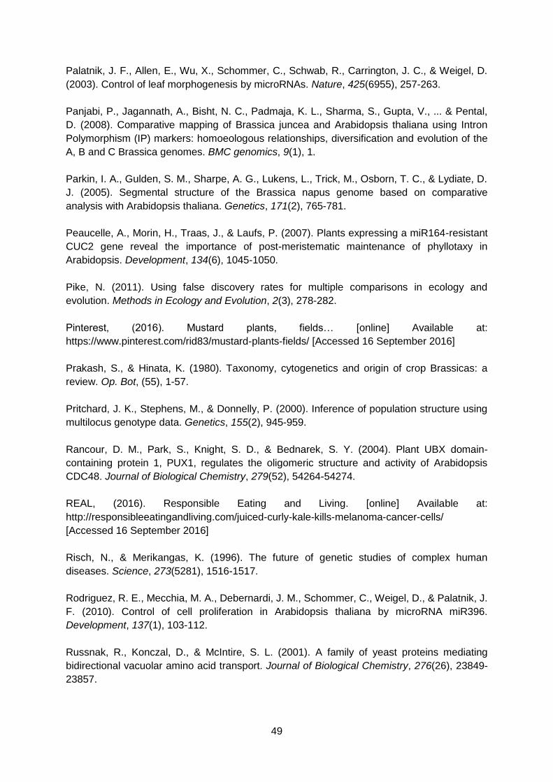
49

Palatnik, J. F., Allen, E., Wu, X., Schommer, C., Schwab, R., Carrington, J. C., & Weigel, D.

(2003). Control of leaf morphogenesis by microRNAs. Nature, 425(6955), 257-263.

Panjabi, P., Jagannath, A., Bisht, N. C., Padmaja, K. L., Sharma, S., Gupta, V., ... & Pental,

D. (2008). Comparative mapping of Brassica juncea and Arabidopsis thaliana using Intron

Polymorphism (IP) markers: homoeologous relationships, diversification and evolution of the

A, B and C Brassica genomes. BMC genomics, 9(1), 1.

Parkin, I. A., Gulden, S. M., Sharpe, A. G., Lukens, L., Trick, M., Osborn, T. C., & Lydiate, D.

J. (2005). Segmental structure of the Brassica napus genome based on comparative

analysis with Arabidopsis thaliana. Genetics, 171(2), 765-781.

Peaucelle, A., Morin, H., Traas, J., & Laufs, P. (2007). Plants expressing a miR164-resistant

CUC2 gene reveal the importance of post-meristematic maintenance of phyllotaxy in

Arabidopsis. Development, 134(6), 1045-1050.

Pike, N. (2011). Using false discovery rates for multiple comparisons in ecology and

evolution. Methods in Ecology and Evolution, 2(3), 278-282.

Pinterest, (2016). Mustard plants, fields… [online] Available at:

https://www.pinterest.com/rid83/mustard-plants-fields/ [Accessed 16 September 2016]

Prakash, S., & Hinata, K. (1980). Taxonomy, cytogenetics and origin of crop Brassicas: a

review. Op. Bot, (55), 1-57.

Pritchard, J. K., Stephens, M., & Donnelly, P. (2000). Inference of population structure using

multilocus genotype data. Genetics, 155(2), 945-959.

Rancour, D. M., Park, S., Knight, S. D., & Bednarek, S. Y. (2004). Plant UBX domain-

containing protein 1, PUX1, regulates the oligomeric structure and activity of Arabidopsis

CDC48. Journal of Biological Chemistry, 279(52), 54264-54274.

REAL, (2016). Responsible Eating and Living. [online] Available at:

http://responsibleeatingandliving.com/juiced-curly-kale-kills-melanoma-cancer-cells/

[Accessed 16 September 2016]

Risch, N., & Merikangas, K. (1996). The future of genetic studies of complex human

diseases. Science, 273(5281), 1516-1517.

Rodriguez, R. E., Mecchia, M. A., Debernardi, J. M., Schommer, C., Weigel, D., & Palatnik, J.

F. (2010). Control of cell proliferation in Arabidopsis thaliana by microRNA miR396.

Development, 137(1), 103-112.

Russnak, R., Konczal, D., & McIntire, S. L. (2001). A family of yeast proteins mediating

bidirectional vacuolar amino acid transport. Journal of Biological Chemistry, 276(26), 23849-

23857.

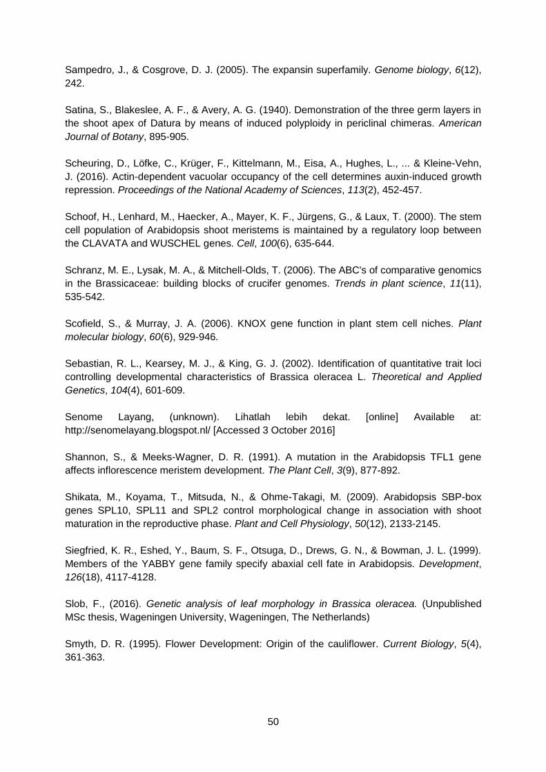
50

Sampedro, J., & Cosgrove, D. J. (2005). The expansin superfamily. Genome biology, 6(12),

242.

Satina, S., Blakeslee, A. F., & Avery, A. G. (1940). Demonstration of the three germ layers in

the shoot apex of Datura by means of induced polyploidy in periclinal chimeras. American

Journal of Botany, 895-905.

Scheuring, D., Löfke, C., Krüger, F., Kittelmann, M., Eisa, A., Hughes, L., ... & Kleine-Vehn,

J. (2016). Actin-dependent vacuolar occupancy of the cell determines auxin-induced growth

repression. Proceedings of the National Academy of Sciences, 113(2), 452-457.

Schoof, H., Lenhard, M., Haecker, A., Mayer, K. F., Jürgens, G., & Laux, T. (2000). The stem

cell population of Arabidopsis shoot meristems is maintained by a regulatory loop between

the CLAVATA and WUSCHEL genes. Cell, 100(6), 635-644.

Schranz, M. E., Lysak, M. A., & Mitchell-Olds, T. (2006). The ABC's of comparative genomics

in the Brassicaceae: building blocks of crucifer genomes. Trends in plant science, 11(11),

535-542.

Scofield, S., & Murray, J. A. (2006). KNOX gene function in plant stem cell niches. Plant

molecular biology, 60(6), 929-946.

Sebastian, R. L., Kearsey, M. J., & King, G. J. (2002). Identification of quantitative trait loci

controlling developmental characteristics of Brassica oleracea L. Theoretical and Applied

Genetics, 104(4), 601-609.

Senome Layang, (unknown). Lihatlah lebih dekat. [online] Available at:

http://senomelayang.blogspot.nl/ [Accessed 3 October 2016]

Shannon, S., & Meeks-Wagner, D. R. (1991). A mutation in the Arabidopsis TFL1 gene

affects inflorescence meristem development. The Plant Cell, 3(9), 877-892.

Shikata, M., Koyama, T., Mitsuda, N., & Ohme-Takagi, M. (2009). Arabidopsis SBP-box

genes SPL10, SPL11 and SPL2 control morphological change in association with shoot

maturation in the reproductive phase. Plant and Cell Physiology, 50(12), 2133-2145.

Siegfried, K. R., Eshed, Y., Baum, S. F., Otsuga, D., Drews, G. N., & Bowman, J. L. (1999).

Members of the YABBY gene family specify abaxial cell fate in Arabidopsis. Development,

126(18), 4117-4128.

Slob, F., (2016). Genetic analysis of leaf morphology in Brassica oleracea. (Unpublished

MSc thesis, Wageningen University, Wageningen, The Netherlands)

Smyth, D. R. (1995). Flower Development: Origin of the cauliflower. Current Biology, 5(4),

361-363.

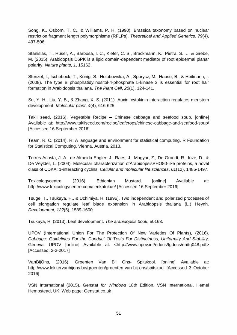
51

Song, K., Osborn, T. C., & Williams, P. H. (1990). Brassica taxonomy based on nuclear

restriction fragment length polymorphisms (RFLPs). Theoretical and Applied Genetics, 79(4),

497-506.

Stanislas, T., Hüser, A., Barbosa, I. C., Kiefer, C. S., Brackmann, K., Pietra, S., ... & Grebe,

M. (2015). Arabidopsis D6PK is a lipid domain-dependent mediator of root epidermal planar

polarity. Nature plants, 1, 15162.

Stenzel, I., Ischebeck, T., König, S., Hołubowska, A., Sporysz, M., Hause, B., & Heilmann, I.

(2008). The type B phosphatidylinositol-4-phosphate 5-kinase 3 is essential for root hair

formation in Arabidopsis thaliana. The Plant Cell, 20(1), 124-141.

Su, Y. H., Liu, Y. B., & Zhang, X. S. (2011). Auxin–cytokinin interaction regulates meristem

development. Molecular plant, 4(4), 616-625.

Takii seed, (2016). Vegetable Recipe – Chinese cabbage and seafood soup. [online]

Available at: http://www.takiiseed.com/recipe/leafcrops/chinese-cabbage-and-seafood-soup/

[Accessed 16 September 2016]

Team, R. C. (2014). R: A language and environment for statistical computing. R Foundation

for Statistical Computing, Vienna, Austria. 2013.

Torres Acosta, J. A., de Almeida Engler, J., Raes, J., Magyar, Z., De Groodt, R., Inzé, D., &

De Veylder, L. (2004). Molecular characterization ofArabidopsisPHO80-like proteins, a novel

class of CDKA; 1-interacting cyclins. Cellular and molecular life sciences, 61(12), 1485-1497.

Toxicologycentre, (2016). Ethiopian Mustard. [online] Available at:

http://www.toxicologycentre.com/cenkatukue/ [Accessed 16 September 2016]

Tsuge, T., Tsukaya, H., & Uchimiya, H. (1996). Two independent and polarized processes of

cell elongation regulate leaf blade expansion in Arabidopsis thaliana (L.) Heynh.

Development, 122(5), 1589-1600.

Tsukaya, H. (2013). Leaf development. The arabidopsis book, e0163.

UPOV (International Union For The Protection Of New Varieties Of Plants), (2016).

Cabbage: Guidelines For the Conduct Of Tests For Distinctness, Uniformity And Stability.

Geneva: UPOV [online] Available at: <http://www.upov.int/edocs/tgdocs/en/tg048.pdf>

[Accessed: 2-2-2017]

VanBijOns, (2016). Groenten Van Bij Ons- Spitskool. [online] Available at:

http://www.lekkervanbijons.be/groenten/groenten-van-bij-ons/spitskool [Accessed 3 October

2016]

VSN International (2015). Genstat for Windows 18th Edition. VSN International, Hemel

Hempstead, UK. Web page: Genstat.co.uk

52

Waites, R., & Hudson, A. (1995). phantastica: a gene required for dorsoventrality of leaves in

Antirrhinum majus. Development, 121(7), 2143-2154.

Wang, H., Ngwenyama, N., Liu, Y., Walker, J. C., & Zhang, S. (2007). Stomatal development

and patterning are regulated by environmentally responsive mitogen-activated protein

kinases in Arabidopsis. The Plant Cell, 19(1), 63-73.

Wang, X., Wang, H., Wang, J., Sun, R., Wu, J., Liu, S., ... & Huang, S. (2011). The genome

of the mesopolyploid crop species Brassica rapa. Nature genetics, 43(10), 1035-1039.

Warwick, S. I., Francis, A., & Al-Shehbaz, I. A. (2006). Brassicaceae: species checklist and

database on CD-Rom. Plant Systematics and Evolution, 259(2-4), 249-258.

Warwick, S. I., Mummenhoff, K., Sauder, C. A., Koch, M. A., & Al-Shehbaz, I. A. (2010).

Closing the gaps: phylogenetic relationships in the Brassicaceae based on DNA sequence

data of nuclear ribosomal ITS region. Plant Systematics and Evolution, 285(3-4), 209-232.

Wikipedia, (2016). Rapeseed. [online] Available at: https://en.wikipedia.org/wiki/Rapeseed

[Accessed 16 September 2016]

Wolf, S., Hématy, K., & Höfte, H. (2012). Growth control and cell wall signaling in plants.

Annual review of plant biology, 63, 381-407.

Xu, R., & Li, Y. (2011). Control of final organ size by Mediator complex subunit 25 in

Arabidopsis thaliana. Development, 138(20), 4545-4554.

Yagi, N., Takeda, S., Matsumoto, N., & Okada, K. (2009). VAJ/GFA1/CLO is involved in the

directional control of floral organ growth. Plant and cell physiology, 50(3), 515-527.

Yanai, O., Shani, E., Dolezal, K., Tarkowski, P., Sablowski, R., Sandberg, G., ... & Ori, N.

(2005). Arabidopsis KNOXI proteins activate cytokinin biosynthesis. Current Biology, 15(17),

1566-1571.

Yokoyama, R., & Nishitani, K. (2001). A comprehensive expression analysis of all members

of a gene family encoding cell-wall enzymes allowed us to predict cis-regulatory regions

involved in cell-wall construction in specific organs of Arabidopsis. Plant and Cell Physiology,

42(10), 1025-1033.

Yu, J., Pressoir, G., Briggs, W. H., Bi, I. V., Yamasaki, M., Doebley, J. F., ... & Kresovich, S.

(2006). A unified mixed-model method for association mapping that accounts for multiple

levels of relatedness. Nature genetics, 38(2), 203-208.

Yu, J., Zhao, M., Wang, X., Tong, C., Huang, S., Tehrim, S., ... & Liu, S. (2013). Bolbase: a

comprehensive genomics database for Brassica oleracea. BMC genomics, 14(1), 664.

Zhang, J., Mason, A. S., Wu, J., Liu, S., Zhang, X., Luo, T., ... & Yan, G. (2015). Identification

of putative candidate genes for water stress tolerance in canola (Brassica napus). Frontiers

in plant science, 6, 1058.

53

Zhang, Y., Persson, S., & Giavalisco, P. (2013). Differential regulation of carbon partitioning

by the central growth regulator Target of Rapamycin (TOR). Molecular plant, 6(6), 1731-

1733.

Zhu, C., Gore, M., Buckler, E. S., & Yu, J. (2008). Status and prospects of association

mapping in plants. The plant genome, 1(1), 5-20.

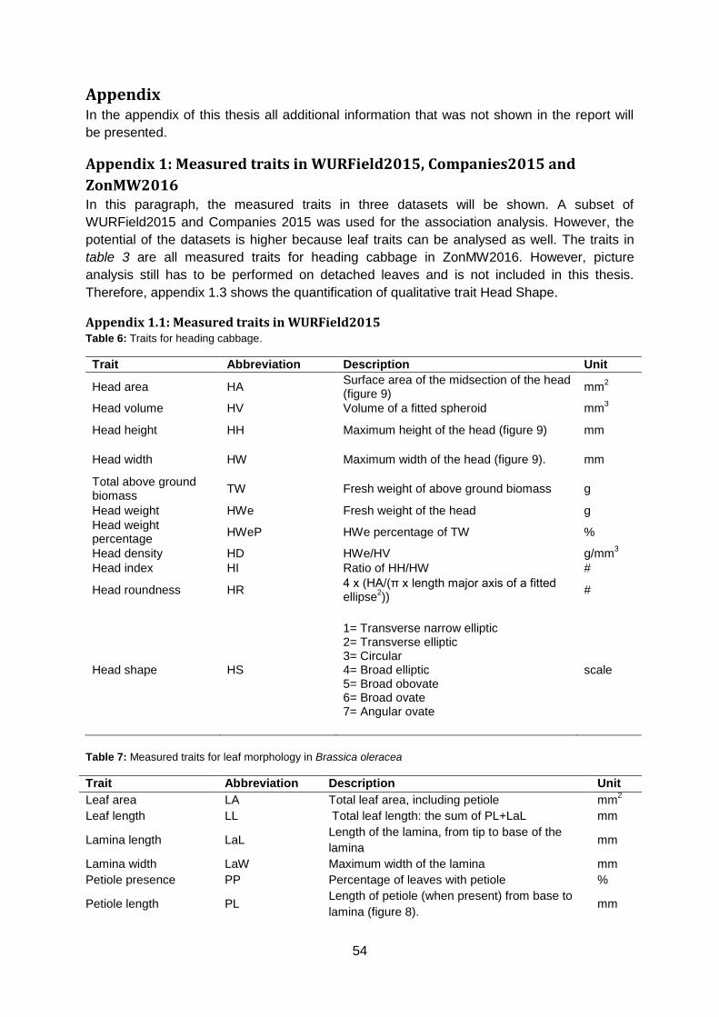
54

Appendix In the appendix of this thesis all additional information that was not shown in the report will

be presented.

Appendix 1: Measured traits in WURField2015, Companies2015 and

ZonMW2016 In this paragraph, the measured traits in three datasets will be shown. A subset of

WURField2015 and Companies 2015 was used for the association analysis. However, the

potential of the datasets is higher because leaf traits can be analysed as well. The traits in

table 3 are all measured traits for heading cabbage in ZonMW2016. However, picture

analysis still has to be performed on detached leaves and is not included in this thesis.

Therefore, appendix 1.3 shows the quantification of qualitative trait Head Shape.

Appendix 1.1: Measured traits in WURField2015 Table 6: Traits for heading cabbage.

Trait Abbreviation Description Unit

Head area HA Surface area of the midsection of the head (figure 9)

mm2

Head volume HV Volume of a fitted spheroid mm3

Head height HH Maximum height of the head (figure 9) mm

Head width HW Maximum width of the head (figure 9). mm

Total above ground biomass

TW Fresh weight of above ground biomass g

Head weight HWe Fresh weight of the head g

Head weight percentage

HWeP HWe percentage of TW %

Head density HD HWe/HV g/mm3

Head index HI Ratio of HH/HW #

Head roundness HR 4 x (HA/(π x length major axis of a fitted ellipse

2))

#

Head shape HS

1= Transverse narrow elliptic 2= Transverse elliptic 3= Circular 4= Broad elliptic 5= Broad obovate 6= Broad ovate 7= Angular ovate

scale

Table 7: Measured traits for leaf morphology in Brassica oleracea

Trait Abbreviation Description Unit

Leaf area LA Total leaf area, including petiole mm2

Leaf length LL Total leaf length: the sum of PL+LaL mm

Lamina length LaL Length of the lamina, from tip to base of the

lamina mm

Lamina width LaW Maximum width of the lamina mm

Petiole presence PP Percentage of leaves with petiole %

Petiole length PL Length of petiole (when present) from base to

lamina (figure 8). mm

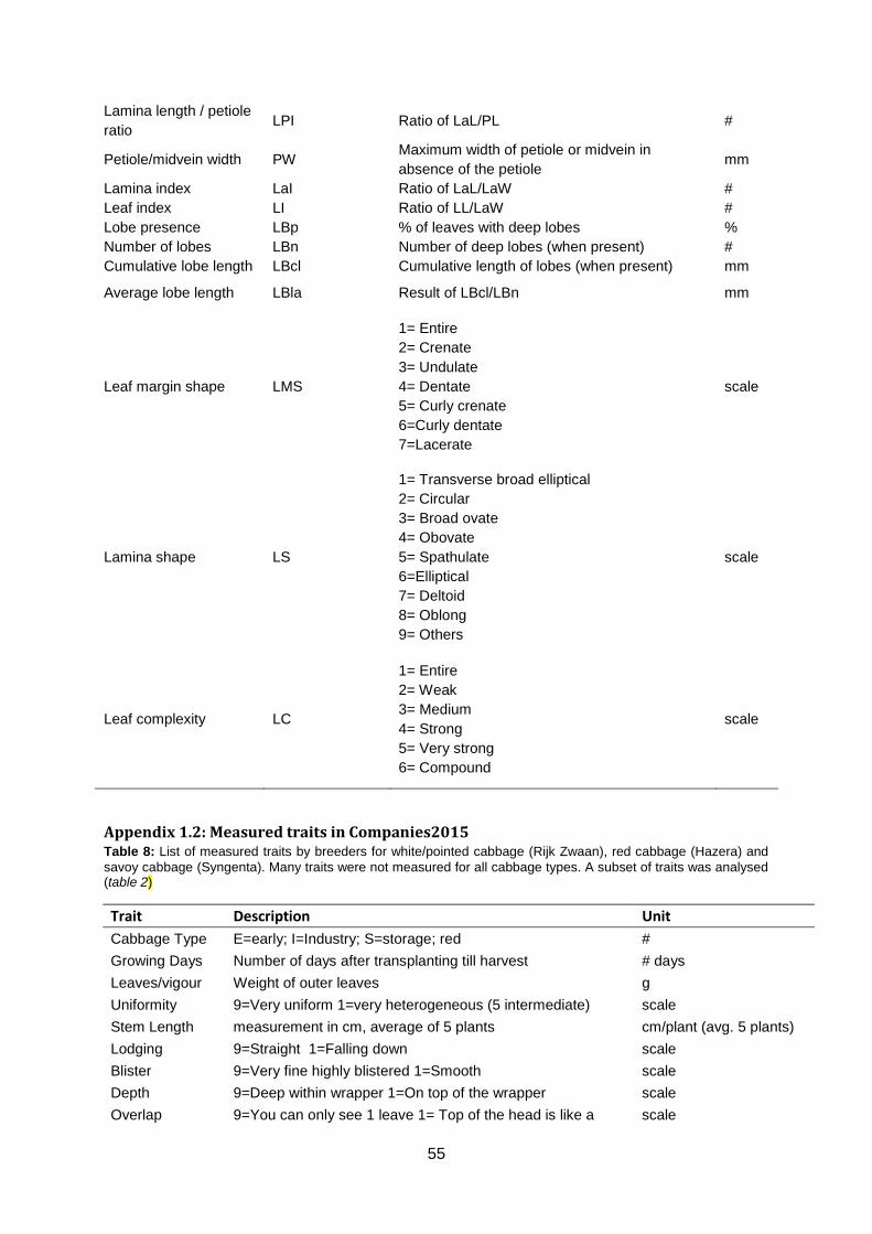
55

Lamina length / petiole

ratio LPI Ratio of LaL/PL #

Petiole/midvein width PW Maximum width of petiole or midvein in

absence of the petiole mm

Lamina index LaI Ratio of LaL/LaW #

Leaf index LI Ratio of LL/LaW #

Lobe presence LBp % of leaves with deep lobes %

Number of lobes LBn Number of deep lobes (when present) #

Cumulative lobe length LBcl Cumulative length of lobes (when present) mm

Average lobe length LBla Result of LBcl/LBn mm

Leaf margin shape LMS

1= Entire

2= Crenate

3= Undulate

4= Dentate

5= Curly crenate

6=Curly dentate

7=Lacerate

scale

Lamina shape LS

1= Transverse broad elliptical

2= Circular

3= Broad ovate

4= Obovate

5= Spathulate

6=Elliptical

7= Deltoid

8= Oblong

9= Others

scale

Leaf complexity LC

1= Entire

2= Weak

3= Medium

4= Strong

5= Very strong

6= Compound

scale

Appendix 1.2: Measured traits in Companies2015 Table 8: List of measured traits by breeders for white/pointed cabbage (Rijk Zwaan), red cabbage (Hazera) and

savoy cabbage (Syngenta). Many traits were not measured for all cabbage types. A subset of traits was analysed (table 2)

Trait Description Unit

Cabbage Type E=early; I=Industry; S=storage; red #

Growing Days Number of days after transplanting till harvest # days

Leaves/vigour Weight of outer leaves g

Uniformity 9=Very uniform 1=very heterogeneous (5 intermediate) scale

Stem Length measurement in cm, average of 5 plants cm/plant (avg. 5 plants)

Lodging 9=Straight 1=Falling down scale

Blister 9=Very fine highly blistered 1=Smooth scale

Depth 9=Deep within wrapper 1=On top of the wrapper scale

Overlap 9=You can only see 1 leave 1= Top of the head is like a scale

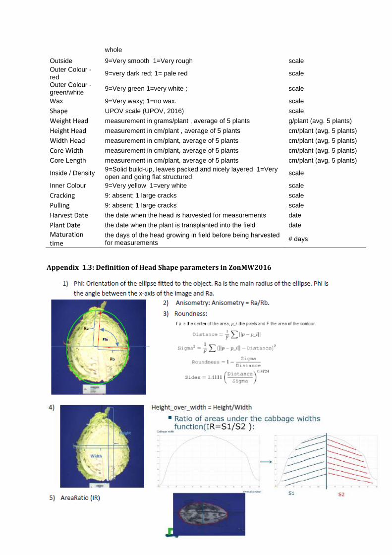
56

whole

Outside 9=Very smooth 1=Very rough scale

Outer Colour - red

9=very dark red; 1= pale red scale

Outer Colour - green/white

9=Very green 1=very white ; scale

Wax 9=Very waxy; 1=no wax. scale

Shape UPOV scale (UPOV, 2016) scale

Weight Head measurement in grams/plant , average of 5 plants g/plant (avg. 5 plants)

Height Head measurement in cm/plant , average of 5 plants cm/plant (avg. 5 plants)

Width Head measurement in cm/plant, average of 5 plants cm/plant (avg. 5 plants)

Core Width measurement in cm/plant, average of 5 plants cm/plant (avg. 5 plants)

Core Length measurement in cm/plant, average of 5 plants cm/plant (avg. 5 plants)

Inside / Density 9=Solid build-up, leaves packed and nicely layered 1=Very open and going flat structured

scale

Inner Colour 9=Very yellow 1=very white scale

Cracking 9: absent; 1 large cracks scale

Pulling 9: absent; 1 large cracks scale

Harvest Date the date when the head is harvested for measurements date

Plant Date the date when the plant is transplanted into the field date

Maturation time

the days of the head growing in field before being harvested for measurements

# days

Appendix 1.3: Definition of Head Shape parameters in ZonMW2016

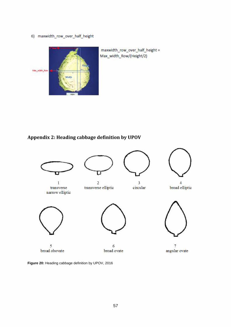
57

Appendix 2: Heading cabbage definition by UPOV

Figure 20: Heading cabbage definition by UPOV, 2016

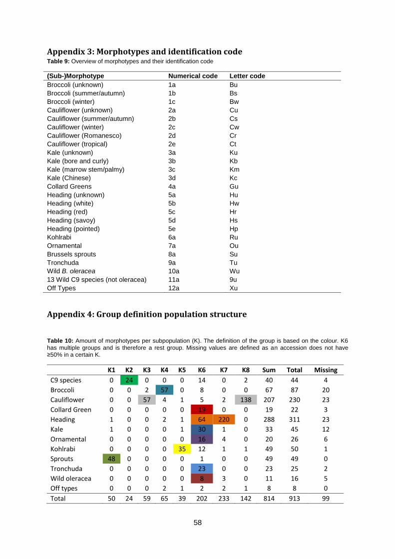
58

Appendix 3: Morphotypes and identification code Table 9: Overview of morphotypes and their identification code

(Sub-)Morphotype Numerical code Letter code

Broccoli (unknown) 1a Bu

Broccoli (summer/autumn) 1b Bs

Broccoli (winter) 1c Bw

Cauliflower (unknown) 2a Cu

Cauliflower (summer/autumn) 2b Cs

Cauliflower (winter) 2c Cw

Cauliflower (Romanesco) 2d Cr

Cauliflower (tropical) 2e Ct

Kale (unknown) 3a Ku

Kale (bore and curly) 3b Kb

Kale (marrow stem/palmy) 3c Km

Kale (Chinese) 3d Kc

Collard Greens 4a Gu

Heading (unknown) 5a Hu

Heading (white) 5b Hw

Heading (red) 5c Hr

Heading (savoy) 5d Hs

Heading (pointed) 5e Hp

Kohlrabi 6a Ru

Ornamental 7a Ou

Brussels sprouts 8a Su

Tronchuda 9a Tu

Wild B. oleracea 10a Wu

13 Wild C9 species (not oleracea) 11a 9u

Off Types 12a Xu

Appendix 4: Group definition population structure Table 10: Amount of morphotypes per subpopulation (K). The definition of the group is based on the colour. K6

has multiple groups and is therefore a rest group. Missing values are defined as an accession does not have ≥50% in a certain K.

K1 K2 K3 K4 K5 K6 K7 K8 Sum Total Missing

C9 species 0 24 0 0 0 14 0 2 40 44 4

Broccoli 0 0 2 57 0 8 0 0 67 87 20

Cauliflower 0 0 57 4 1 5 2 138 207 230 23

Collard Green 0 0 0 0 0 19 0 0 19 22 3

Heading 1 0 0 2 1 64 220 0 288 311 23

Kale 1 0 0 0 1 30 1 0 33 45 12

Ornamental 0 0 0 0 0 16 4 0 20 26 6

Kohlrabi 0 0 0 0 35 12 1 1 49 50 1

Sprouts 48 0 0 0 0 1 0 0 49 49 0

Tronchuda 0 0 0 0 0 23 0 0 23 25 2

Wild oleracea 0 0 0 0 0 8 3 0 11 16 5

Off types 0 0 0 2 1 2 2 1 8 8 0

Total 50 24 59 65 39 202 233 142 814 913 99

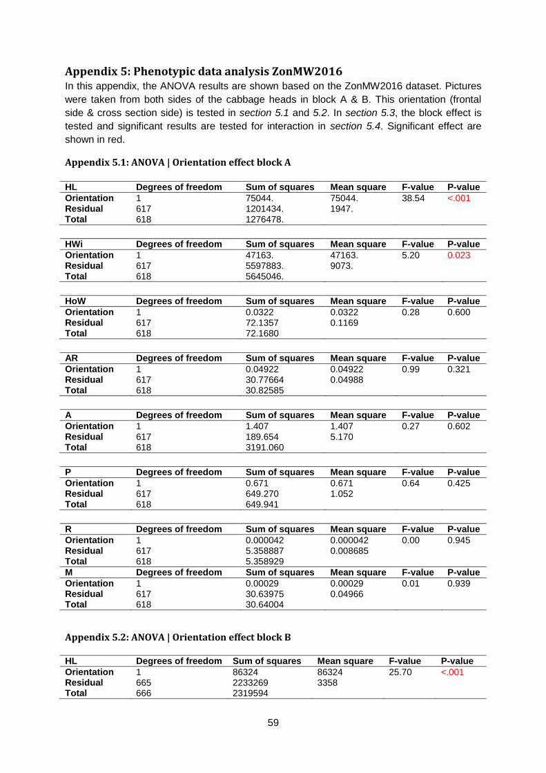
59

Appendix 5: Phenotypic data analysis ZonMW2016 In this appendix, the ANOVA results are shown based on the ZonMW2016 dataset. Pictures

were taken from both sides of the cabbage heads in block A & B. This orientation (frontal

side & cross section side) is tested in section 5.1 and 5.2. In section 5.3, the block effect is

tested and significant results are tested for interaction in section 5.4. Significant effect are

shown in red.

Appendix 5.1: ANOVA | Orientation effect block A

HL Degrees of freedom Sum of squares Mean square F-value P-value

Orientation 1 75044. 75044. 38.54 <.001 Residual 617 1201434. 1947. Total 618 1276478.

HWi Degrees of freedom Sum of squares Mean square F-value P-value

Orientation 1 47163. 47163. 5.20 0.023 Residual 617 5597883. 9073. Total 618 5645046.

HoW Degrees of freedom Sum of squares Mean square F-value P-value

Orientation 1 0.0322 0.0322 0.28 0.600 Residual 617 72.1357 0.1169 Total 618 72.1680

AR Degrees of freedom Sum of squares Mean square F-value P-value

Orientation 1 0.04922 0.04922 0.99 0.321 Residual 617 30.77664 0.04988 Total 618 30.82585

A Degrees of freedom Sum of squares Mean square F-value P-value

Orientation 1 1.407 1.407 0.27 0.602 Residual 617 189.654 5.170 Total 618 3191.060

P Degrees of freedom Sum of squares Mean square F-value P-value

Orientation 1 0.671 0.671 0.64 0.425 Residual 617 649.270 1.052 Total 618 649.941

R Degrees of freedom Sum of squares Mean square F-value P-value

Orientation 1 0.000042 0.000042 0.00 0.945 Residual 617 5.358887 0.008685 Total 618 5.358929

M Degrees of freedom Sum of squares Mean square F-value P-value

Orientation 1 0.00029 0.00029 0.01 0.939 Residual 617 30.63975 0.04966 Total 618 30.64004

Appendix 5.2: ANOVA | Orientation effect block B

HL Degrees of freedom Sum of squares Mean square F-value P-value

Orientation 1 86324 86324 25.70 <.001 Residual 665 2233269 3358 Total 666 2319594

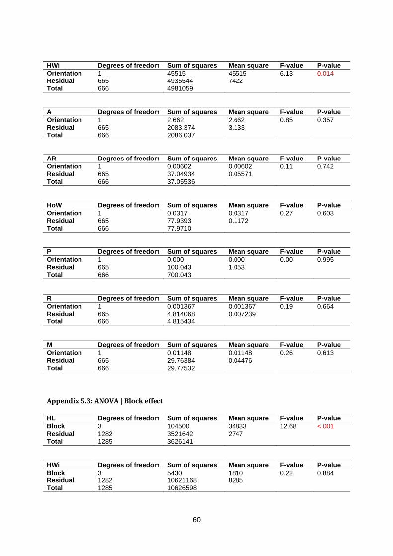
60

HWi Degrees of freedom Sum of squares Mean square F-value P-value

Orientation 1 45515 45515 6.13 0.014 Residual 665 4935544 7422 Total 666 4981059

A Degrees of freedom Sum of squares Mean square F-value P-value

Orientation 1 2.662 2.662 0.85 0.357 Residual 665 2083.374 3.133 Total 666 2086.037

AR Degrees of freedom Sum of squares Mean square F-value P-value

Orientation 1 0.00602 0.00602 0.11 0.742 Residual 665 37.04934 0.05571 Total 666 37.05536

HoW Degrees of freedom Sum of squares Mean square F-value P-value

Orientation 1 0.0317 0.0317 0.27 0.603 Residual 665 77.9393 0.1172 Total 666 77.9710

P Degrees of freedom Sum of squares Mean square F-value P-value

Orientation 1 0.000 0.000 0.00 0.995 Residual 665 100.043 1.053 Total 666 700.043

R Degrees of freedom Sum of squares Mean square F-value P-value

Orientation 1 0.001367 0.001367 0.19 0.664 Residual 665 4.814068 0.007239 Total 666 4.815434

M Degrees of freedom Sum of squares Mean square F-value P-value

Orientation 1 0.01148 0.01148 0.26 0.613 Residual 665 29.76384 0.04476 Total 666 29.77532

Appendix 5.3: ANOVA | Block effect

HL Degrees of freedom Sum of squares Mean square F-value P-value

Block 3 104500 34833 12.68 <.001 Residual 1282 3521642 2747 Total 1285 3626141

HWi Degrees of freedom Sum of squares Mean square F-value P-value

Block 3 5430 1810 0.22 0.884 Residual 1282 10621168 8285 Total 1285 10626598

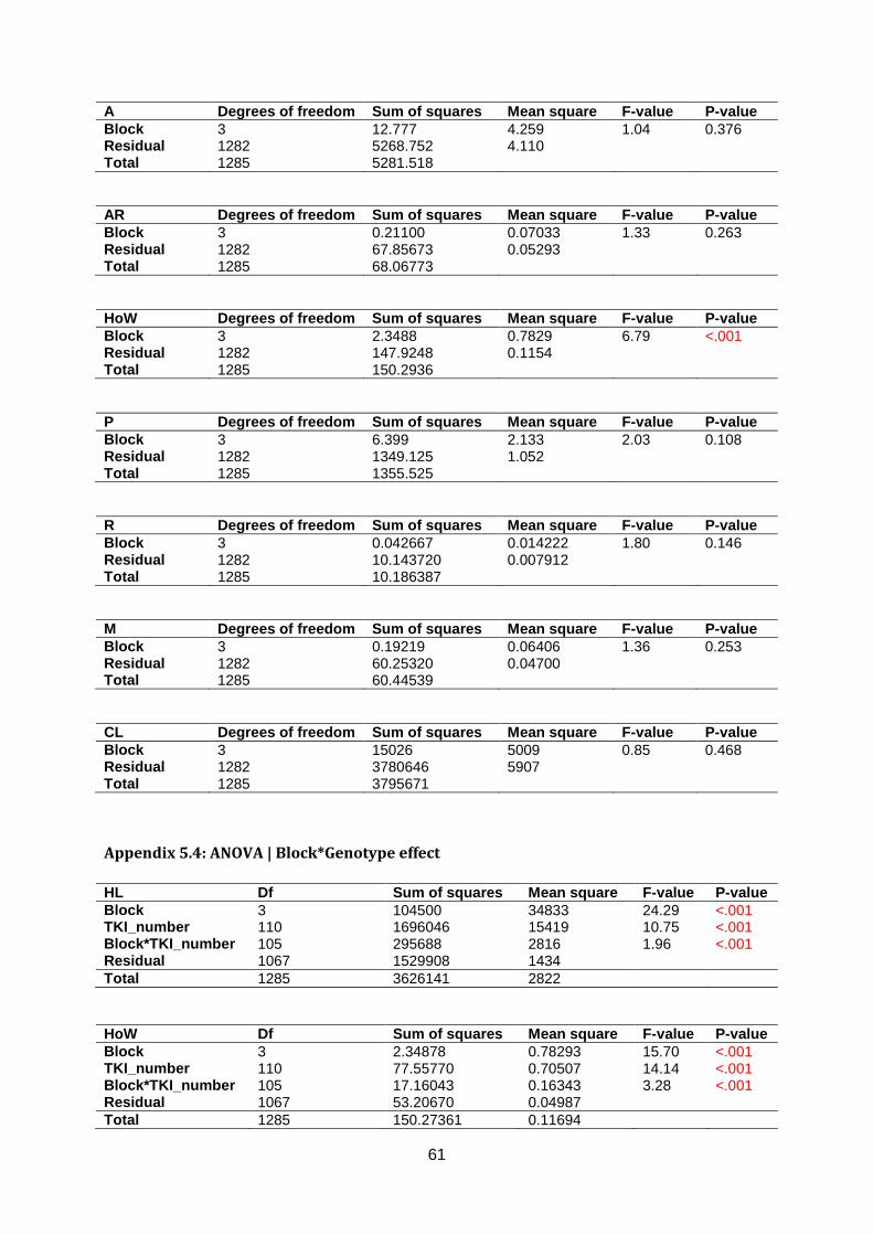
61

A Degrees of freedom Sum of squares Mean square F-value P-value

Block 3 12.777 4.259 1.04 0.376 Residual 1282 5268.752 4.110 Total 1285 5281.518

AR Degrees of freedom Sum of squares Mean square F-value P-value

Block 3 0.21100 0.07033 1.33 0.263 Residual 1282 67.85673 0.05293 Total 1285 68.06773

HoW Degrees of freedom Sum of squares Mean square F-value P-value

Block 3 2.3488 0.7829 6.79 <.001 Residual 1282 147.9248 0.1154 Total 1285 150.2936

P Degrees of freedom Sum of squares Mean square F-value P-value

Block 3 6.399 2.133 2.03 0.108 Residual 1282 1349.125 1.052 Total 1285 1355.525

R Degrees of freedom Sum of squares Mean square F-value P-value

Block 3 0.042667 0.014222 1.80 0.146 Residual 1282 10.143720 0.007912 Total 1285 10.186387

M Degrees of freedom Sum of squares Mean square F-value P-value

Block 3 0.19219 0.06406 1.36 0.253 Residual 1282 60.25320 0.04700 Total 1285 60.44539

CL Degrees of freedom Sum of squares Mean square F-value P-value

Block 3 15026 5009 0.85 0.468 Residual 1282 3780646 5907 Total 1285 3795671

Appendix 5.4: ANOVA | Block*Genotype effect

HL Df Sum of squares Mean square F-value P-value

Block 3 104500 34833 24.29 <.001 TKI_number 110 1696046 15419 10.75 <.001 Block*TKI_number 105 295688 2816 1.96 <.001 Residual 1067 1529908 1434

Total 1285 3626141 2822

HoW Df Sum of squares Mean square F-value P-value

Block 3 2.34878 0.78293 15.70 <.001 TKI_number 110 77.55770 0.70507 14.14 <.001 Block*TKI_number 105 17.16043 0.16343 3.28 <.001 Residual 1067 53.20670 0.04987

Total 1285 150.27361 0.11694

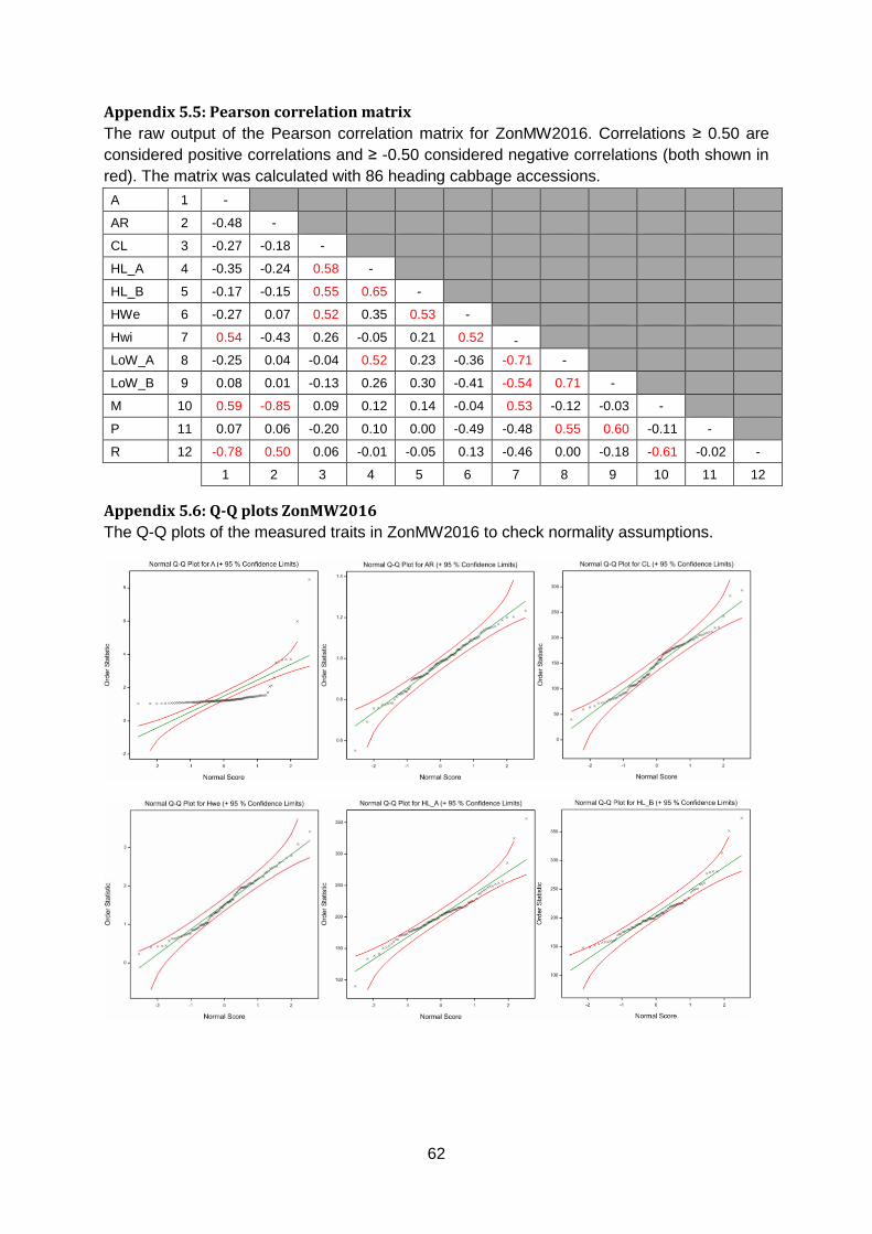
62

Appendix 5.5: Pearson correlation matrix

The raw output of the Pearson correlation matrix for ZonMW2016. Correlations ≥ 0.50 are

considered positive correlations and ≥ -0.50 considered negative correlations (both shown in

red). The matrix was calculated with 86 heading cabbage accessions.

A 1 -

AR 2 -0.48 -

CL 3 -0.27 -0.18 -

HL_A 4 -0.35 -0.24 0.58 -

HL_B 5 -0.17 -0.15 0.55 0.65 -

HWe 6 -0.27 0.07 0.52 0.35 0.53 -

Hwi 7 0.54 -0.43 0.26 -0.05 0.21 0.52 -

LoW_A 8 -0.25 0.04 -0.04 0.52 0.23 -0.36 -0.71 -

LoW_B 9 0.08 0.01 -0.13 0.26 0.30 -0.41 -0.54 0.71 -

M 10 0.59 -0.85 0.09 0.12 0.14 -0.04 0.53 -0.12 -0.03 -

P 11 0.07 0.06 -0.20 0.10 0.00 -0.49 -0.48 0.55 0.60 -0.11 -

R 12 -0.78 0.50 0.06 -0.01 -0.05 0.13 -0.46 0.00 -0.18 -0.61 -0.02 -

1 2 3 4 5 6 7 8 9 10 11 12

Appendix 5.6: Q-Q plots ZonMW2016

The Q-Q plots of the measured traits in ZonMW2016 to check normality assumptions.

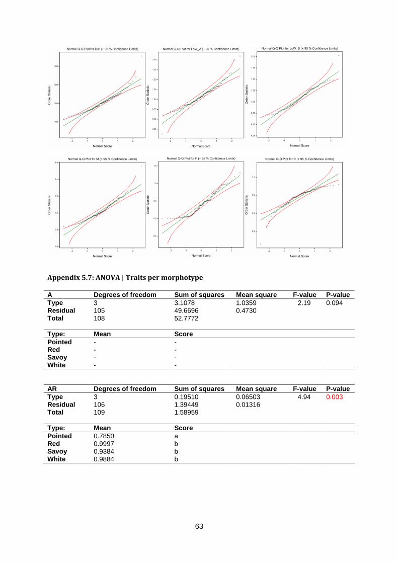
63

Appendix 5.7: ANOVA | Traits per morphotype

A Degrees of freedom Sum of squares Mean square F-value P-value

Type 3 3.1078 1.0359 2.19 0.094 Residual 105 49.6696 0.4730 Total 108 52.7772

Type: Mean Score

Pointed - - Red - - Savoy - - White - -

AR Degrees of freedom Sum of squares Mean square F-value P-value

Type 3 0.19510 0.06503 4.94 0.003 Residual 106 1.39449 0.01316 Total 109 1.58959

Type: Mean Score

Pointed 0.7850 a Red 0.9997 b Savoy 0.9384 b White 0.9884 b

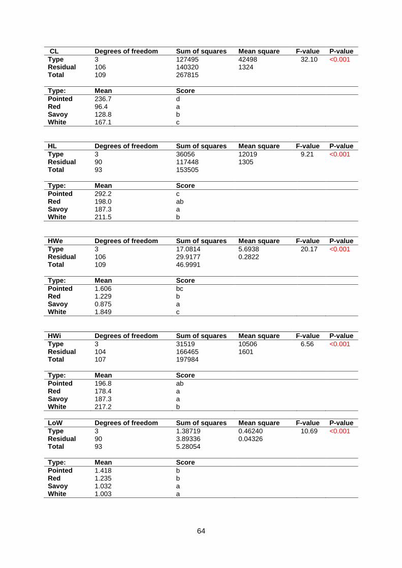
64

CL Degrees of freedom Sum of squares Mean square F-value P-value

Type 3 127495 42498 32.10 <0.001 Residual 106 140320 1324 Total 109 267815

Type: Mean Score

Pointed 236.7 d Red 96.4 a Savoy 128.8 b White 167.1 c

HL Degrees of freedom Sum of squares Mean square F-value P-value

Type 3 36056 12019 9.21 <0.001 Residual 90 117448 1305 Total 93 153505

Type: Mean Score

Pointed 292.2 c Red 198.0 ab Savoy 187.3 a White 211.5 b

HWe Degrees of freedom Sum of squares Mean square F-value P-value

Type 3 17.0814 5.6938 20.17 <0.001 Residual 106 29.9177 0.2822 Total 109 46.9991

Type: Mean Score

Pointed 1.606 bc Red 1.229 b Savoy 0.875 a White 1.849 c

HWi Degrees of freedom Sum of squares Mean square F-value P-value

Type 3 31519 10506 6.56 <0.001 Residual 104 166465 1601 Total 107 197984

Type: Mean Score

Pointed 196.8 ab Red 178.4 a Savoy 187.3 a White 217.2 b

LoW Degrees of freedom Sum of squares Mean square F-value P-value

Type 3 1.38719 0.46240 10.69 <0.001 Residual 90 3.89336 0.04326 Total 93 5.28054

Type: Mean Score

Pointed 1.418 b Red 1.235 b Savoy 1.032 a White 1.003 a

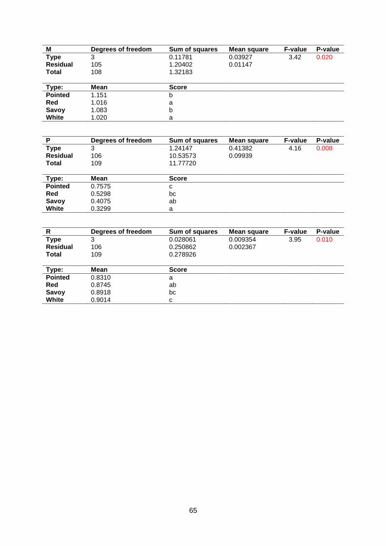
65

M Degrees of freedom Sum of squares Mean square F-value P-value

Type 3 0.11781 0.03927 3.42 0.020 Residual 105 1.20402 0.01147 Total 108 1.32183

Type: Mean Score

Pointed 1.151 b Red 1.016 a Savoy 1.083 b White 1.020 a

P Degrees of freedom Sum of squares Mean square F-value P-value

Type 3 1.24147 0.41382 4.16 0.008 Residual 106 10.53573 0.09939 Total 109 11.77720

Type: Mean Score

Pointed 0.7575 c Red 0.5298 bc Savoy 0.4075 ab White 0.3299 a

R Degrees of freedom Sum of squares Mean square F-value P-value

Type 3 0.028061 0.009354 3.95 0.010 Residual 106 0.250862 0.002367 Total 109 0.278926

Type: Mean Score

Pointed 0.8310 a Red 0.8745 ab Savoy 0.8918 bc White 0.9014 c

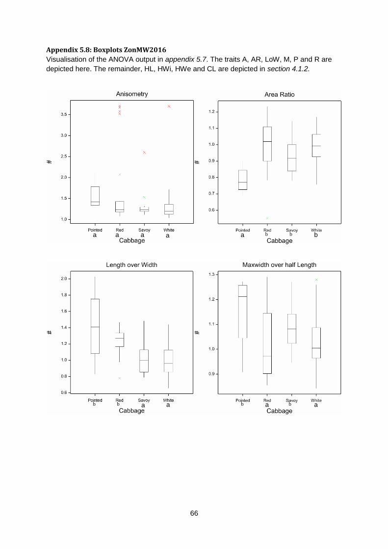
66

Appendix 5.8: Boxplots ZonMW2016

Visualisation of the ANOVA output in appendix 5.7. The traits A, AR, LoW, M, P and R are

depicted here. The remainder, HL, HWi, HWe and CL are depicted in section 4.1.2.

a a a a b a b b

b b a a a b a b

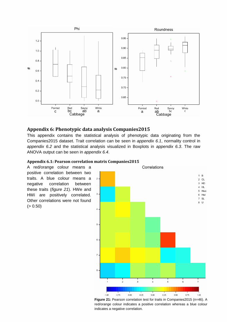
67

Appendix 6: Phenotypic data analysis Companies2015 This appendix contains the statistical analysis of phenotypic data originating from the

Companies2015 dataset. Trait correlation can be seen in appendix 6.1, normality control in

appendix 6.2 and the statistical analysis visualized in Boxplots in appendix 6.3. The raw

ANOVA output can be seen in appendix 6.4.

Appendix 6.1: Pearson correlation matrix Companies2015

A red/orange colour means a

positive correlation between two

traits. A blue colour means a

negative correlation between

these traits (figure 21). HWe and

HWi are positively correlated.

Other correlations were not found

(> 0.50)

Figure 21: Pearson correlation test for traits in Companies2015 (n=46). A

red/orange colour indicates a positive correlation whereas a blue colour

indicates a negative correlation.

bc c a ab c bc a ab

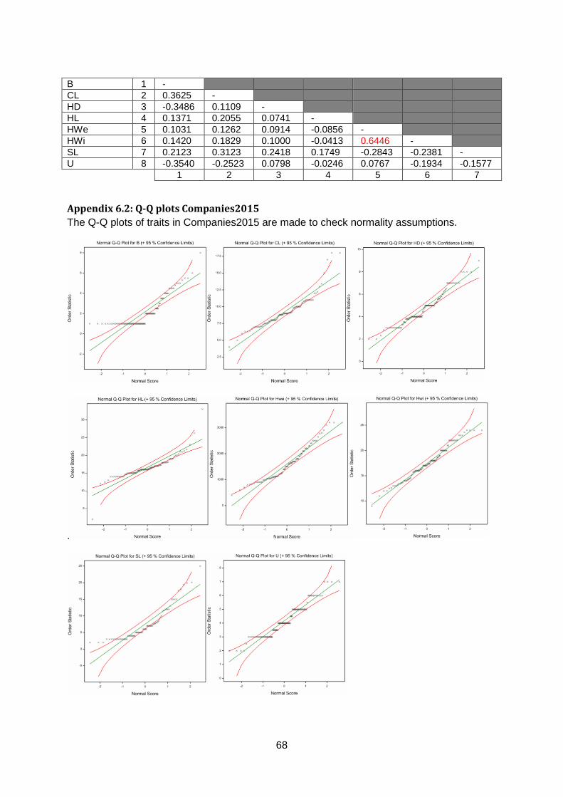
68

B 1 -

CL 2 0.3625 -

HD 3 -0.3486 0.1109 -

HL 4 0.1371 0.2055 0.0741 -

HWe 5 0.1031 0.1262 0.0914 -0.0856 -

HWi 6 0.1420 0.1829 0.1000 -0.0413 0.6446 -

SL 7 0.2123 0.3123 0.2418 0.1749 -0.2843 -0.2381 -

U 8 -0.3540 -0.2523 0.0798 -0.0246 0.0767 -0.1934 -0.1577

1 2 3 4 5 6 7

Appendix 6.2: Q-Q plots Companies2015

The Q-Q plots of traits in Companies2015 are made to check normality assumptions.

.

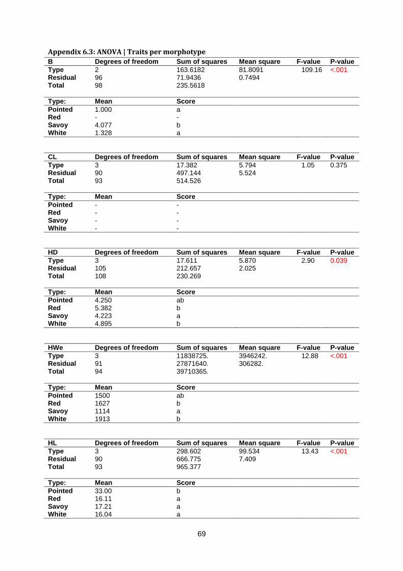
69

Appendix 6.3: ANOVA | Traits per morphotype

B Degrees of freedom Sum of squares Mean square F-value P-value

Type 2 163.6182 81.8091 109.16 <.001 Residual 96 71.9436 0.7494 Total 98 235.5618

Type: Mean Score

Pointed 1.000 a Red - - Savoy 4.077 b White 1.328 a

CL Degrees of freedom Sum of squares Mean square F-value P-value

Type 3 17.382 5.794 1.05 0.375 Residual 90 497.144 5.524 Total 93 514.526

Type: Mean Score

Pointed - - Red - - Savoy - - White - -

HD Degrees of freedom Sum of squares Mean square F-value P-value

Type 3 17.611 5.870 2.90 0.039 Residual 105 212.657 2.025 Total 108 230.269

Type: Mean Score

Pointed 4.250 ab Red 5.382 b Savoy 4.223 a White 4.895 b

HWe Degrees of freedom Sum of squares Mean square F-value P-value

Type 3 11838725. 3946242. 12.88 <.001 Residual 91 27871640. 306282. Total 94 39710365.

Type: Mean Score

Pointed 1500 ab Red 1627 b Savoy 1114 a White 1913 b

HL Degrees of freedom Sum of squares Mean square F-value P-value

Type 3 298.602 99.534 13.43 <.001 Residual 90 666.775 7.409 Total 93 965.377

Type: Mean Score

Pointed 33.00 b Red 16.11 a Savoy 17.21 a White 16.04 a

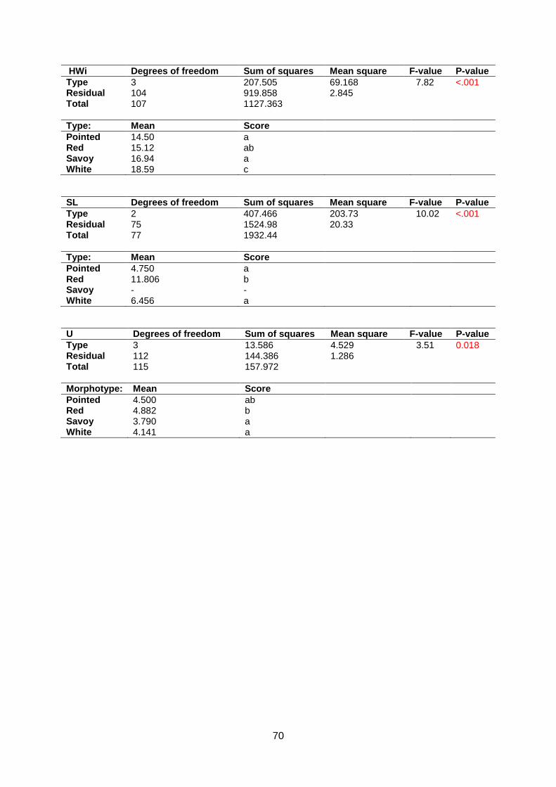
70

HWi Degrees of freedom Sum of squares Mean square F-value P-value

Type 3 207.505 69.168 7.82 <.001 Residual 104 919.858 2.845 Total 107 1127.363

Type: Mean Score

Pointed 14.50 a Red 15.12 ab Savoy 16.94 a White 18.59 c

SL Degrees of freedom Sum of squares Mean square F-value P-value

Type 2 407.466 203.73 10.02 <.001 Residual 75 1524.98 20.33 Total 77 1932.44

Type: Mean Score

Pointed 4.750 a Red 11.806 b Savoy - - White 6.456 a

U Degrees of freedom Sum of squares Mean square F-value P-value

Type 3 13.586 4.529 3.51 0.018 Residual 112 144.386 1.286 Total 115 157.972

Morphotype: Mean Score

Pointed 4.500 ab Red 4.882 b Savoy 3.790 a White 4.141 a

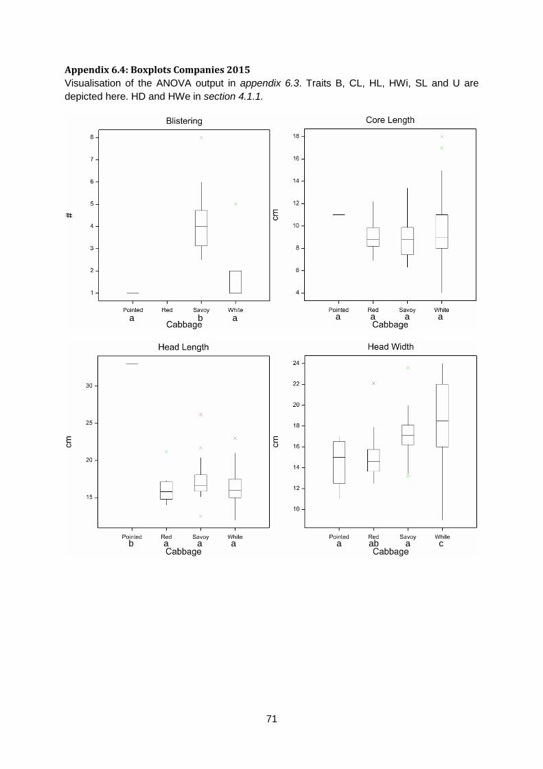
71

Appendix 6.4: Boxplots Companies 2015

Visualisation of the ANOVA output in appendix 6.3. Traits B, CL, HL, HWi, SL and U are

depicted here. HD and HWe in section 4.1.1.

a b a a a a a

a a a b ab a a c

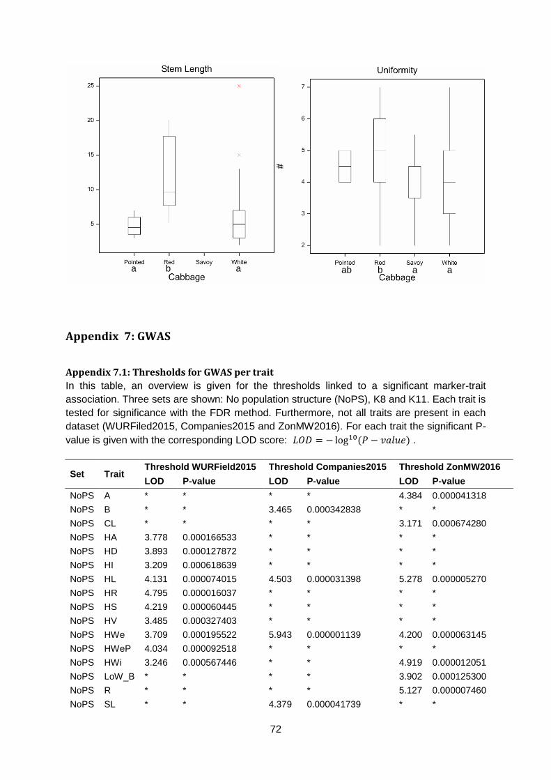
72

Appendix 7: GWAS

Appendix 7.1: Thresholds for GWAS per trait

In this table, an overview is given for the thresholds linked to a significant marker-trait

association. Three sets are shown: No population structure (NoPS), K8 and K11. Each trait is

tested for significance with the FDR method. Furthermore, not all traits are present in each

dataset (WURFiled2015, Companies2015 and ZonMW2016). For each trait the significant P-

value is given with the corresponding LOD score: 𝐿𝑂𝐷 = − log10(𝑃 − 𝑣𝑎𝑙𝑢𝑒) .

Set Trait Threshold WURField2015 Threshold Companies2015 Threshold ZonMW2016

LOD P-value LOD P-value LOD P-value

NoPS A * * * * 4.384 0.000041318

NoPS B * * 3.465 0.000342838 * *

NoPS CL * * * * 3.171 0.000674280

NoPS HA 3.778 0.000166533 * * * *

NoPS HD 3.893 0.000127872 * * * *

NoPS HI 3.209 0.000618639 * * * *

NoPS HL 4.131 0.000074015 4.503 0.000031398 5.278 0.000005270

NoPS HR 4.795 0.000016037 * * * *

NoPS HS 4.219 0.000060445 * * * *

NoPS HV 3.485 0.000327403 * * * *

NoPS HWe 3.709 0.000195522 5.943 0.000001139 4.200 0.000063145

NoPS HWeP 4.034 0.000092518 * * * *

NoPS HWi 3.246 0.000567446 * * 4.919 0.000012051

NoPS LoW_B * * * * 3.902 0.000125300

NoPS R * * * * 5.127 0.000007460

NoPS SL * * 4.379 0.000041739 * *

b a a b ab a a

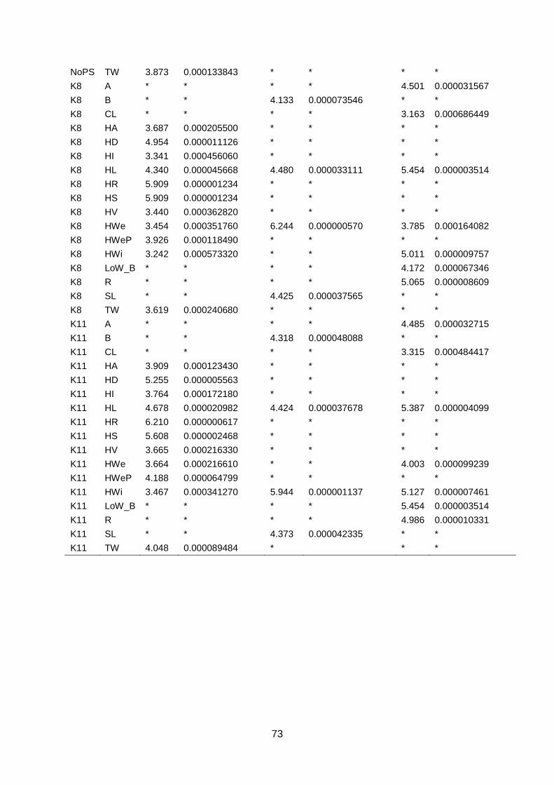
73

NoPS TW 3.873 0.000133843 * * * *

K8 A * * * * 4.501 0.000031567

K8 B * * 4.133 0.000073546 * *

K8 CL * * * * 3.163 0.000686449

K8 HA 3.687 0.000205500 * * * *

K8 HD 4.954 0.000011126 * * * *

K8 HI 3.341 0.000456060 * * * *

K8 HL 4.340 0.000045668 4.480 0.000033111 5.454 0.000003514

K8 HR 5.909 0.000001234 * * * *

K8 HS 5.909 0.000001234 * * * *

K8 HV 3.440 0.000362820 * * * *

K8 HWe 3.454 0.000351760 6.244 0.000000570 3.785 0.000164082

K8 HWeP 3.926 0.000118490 * * * *

K8 HWi 3.242 0.000573320 * * 5.011 0.000009757

K8 LoW_B * * * * 4.172 0.000067346

K8 R * * * * 5.065 0.000008609

K8 SL * * 4.425 0.000037565 * *

K8 TW 3.619 0.000240680 * * * *

K11 A * * * * 4.485 0.000032715

K11 B * * 4.318 0.000048088 * *

K11 CL * * * * 3.315 0.000484417

K11 HA 3.909 0.000123430 * * * *

K11 HD 5.255 0.000005563 * * * *

K11 HI 3.764 0.000172180 * * * *

K11 HL 4.678 0.000020982 4.424 0.000037678 5.387 0.000004099

K11 HR 6.210 0.000000617 * * * *

K11 HS 5.608 0.000002468 * * * *

K11 HV 3.665 0.000216330 * * * *

K11 HWe 3.664 0.000216610 * * 4.003 0.000099239

K11 HWeP 4.188 0.000064799 * * * *

K11 HWi 3.467 0.000341270 5.944 0.000001137 5.127 0.000007461

K11 LoW_B * * * * 5.454 0.000003514

K11 R * * * * 4.986 0.000010331

K11 SL * * 4.373 0.000042335 * *

K11 TW 4.048 0.000089484 * * *

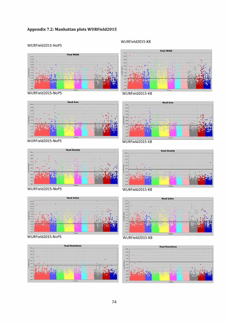
74

Appendix 7.2: Manhattan plots WURField2015

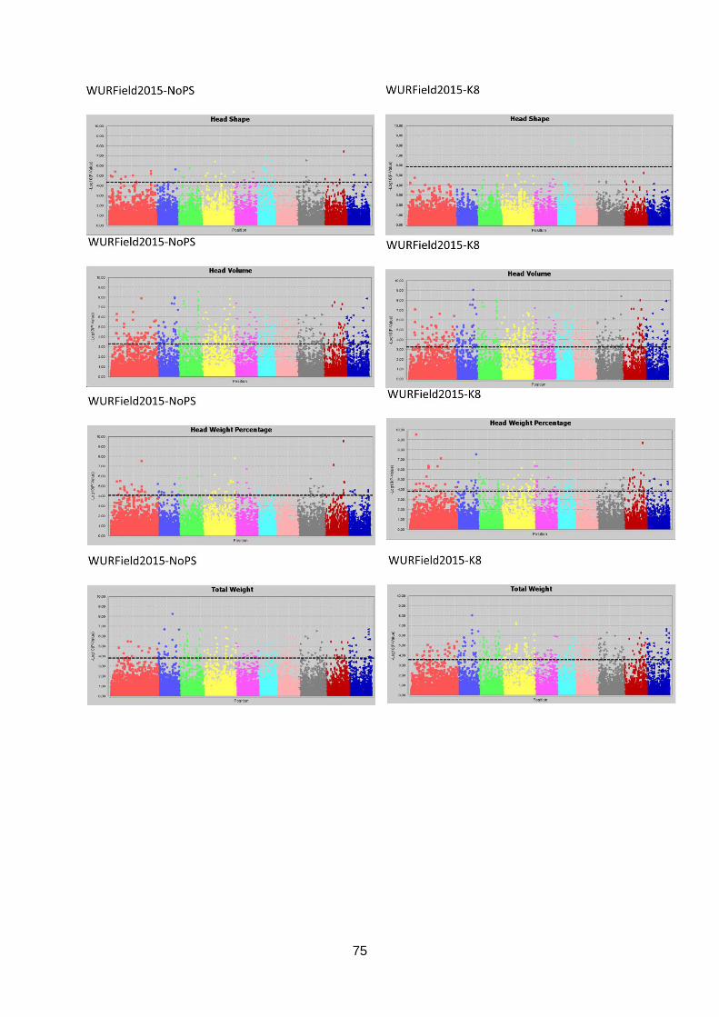
75

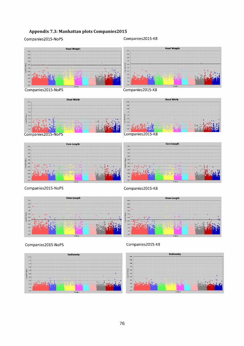
76

Appendix 7.3: Manhattan plots Companies2015

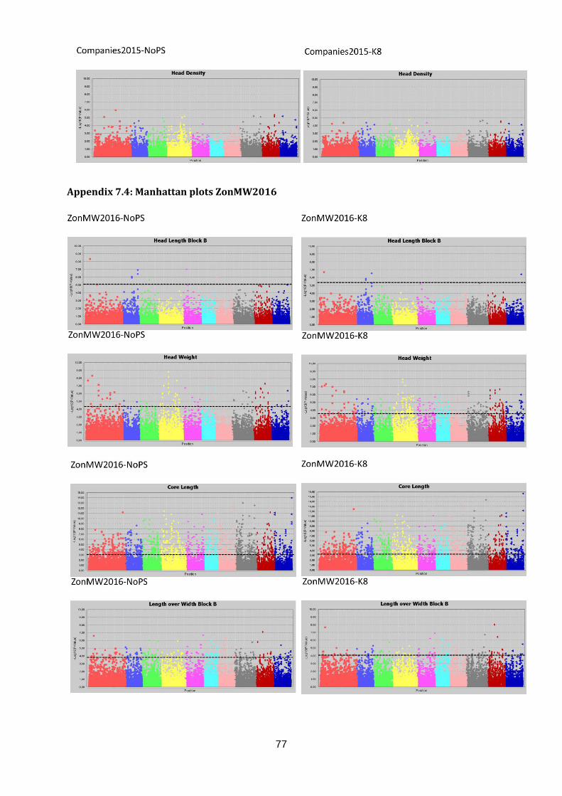
77

Appendix 7.4: Manhattan plots ZonMW2016

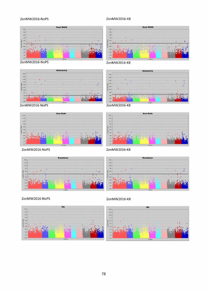
78

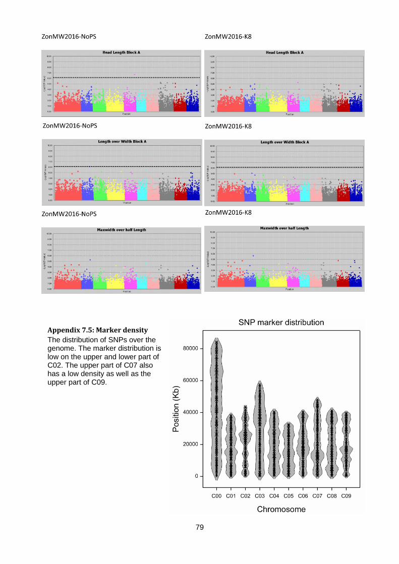
79

Appendix 7.5: Marker density

The distribution of SNPs over the genome. The marker distribution is low on the upper and lower part of C02. The upper part of C07 also has a low density as well as the upper part of C09.