Geographical Information Systems

and

Dynamic Models

Development and application of a

prototype spatial modelling language

WPA van Deursen

PhD-thesis, may 19, 1995Faculty of Spatial SciencesUniversity of UtrechtThe Netherlands

@1995,2000, WPA van DeursenOostzeedijk Beneden 23a3062 VK Rotterdam, The Netherlandswvandeursen@carthago.nl

This publication is also available in paper form. This publication is part of NGS, Netherlands GeographicalStudies.

NGS 190 W P A VAN DEURSEN Geographical Information Systems and Dynamic Models; development and application of a prototype spatial modelling language -- Utrecht 1995: Knag/Faculteit Ruimtelijke Wetenschappen Universiteit Utrecht. 206 pp, 44 figs, 8 tabs. ISBN 90-6809-206-5 Dfl 38,00

Publications of this series can be ordered from KNAG / NETHERLANDS GEOGRAPHICAL STUDIES,P.O.Box 80123, 3508 TC Utrecht, The Netherlands (Fax +31 30 253 5523; E-mail KNAG@geog.uu.nl).

Please refer to this publication as:Van Deursen W.P.A. 1995. Geographical Information Systems and Dynamic Models. Ph.D. thesis, UtrechtUniversity, NGS Publication 190, 198 pp. Electronically available through www.carthago.nl

Please feel free to copy and redistribute this PDF document, provided that no changes are made to the document.

The PCRaster software, which implements the techniques described in this document (although not exactly) isavailable through www.pcraster.nl

Rotterdam, November 2000

Willem van Deursen, wvandeursen@carthago.nl

1 INTRODUCTION

1.1 The use of Geographical Information Systems and dynamic models inphysical geography, ecology and environmental studies

A convenient way to define a Geographical Information System (GIS) is to say that it is a set of computer toolscapable of storing, manipulating, analysing and retrieving geographic information [Burrough, 1986; Maguire,1991]. Several questions arise from this definition. What exactly is geographic information; and what is meantby the sentence 'storing, manipulating and analysing and retrieving geographic information'? Both thesequestions are the cause of much discussion and research in the GIS society. This thesis will touch upon the firstquestion, and will discuss thoroughly an approach for dynamic modelling with GIS. In this context dynamicmodelling can be regarded as a subset of 'manipulating and analysing geographic data'.

Geographic information is information that has a geographic attribute, that is, it is linked to some location. Wecan recognise two main types of geographic information [Goodchild 1992]. The first type relates to the conceptof objects, features that can have a certain set of attributes. It is quite convenient to think of objects as beinggeographically limited in size, and objects are quite often man-made or stem from classification of the world. Incontrast to the object-related information, there is the concept of fields. Fields are not geographically limited, butmay have different attribute values at different locations. Elevation is an example of a field. The attribute 'metresabove sea level' is defined over the total area, but may take different values at different locations. The majordiscussion in the GIS world about the vector and raster approaches is mainly along the lines of the concept ofobjects and fields.

The second important aspect of the definition of GIS is the capability for manipulating and analysing thegeographic information. Manipulating and analysing refer to retrieving data from the geographical database andcreating new information by combining this data. The analysis and manipulation are done through commandsand functions. A major milestone in the development of GIS capabilities for manipulating and analysinggeographic information has been the formulation of Map Algebra and Cartographic Modelling [Tomlin andBerry, 1979; Tomlin, 1983; Berry 1987]. Map Algebra is an integrated set of functions and commands foranalysing and manipulating geographic information. The major significance of Map Algebra is that it does notprovide ad hoc operations and functions for all possible geographic analyses that could be conceived, but insteadprovides limited generic functionality, which can be used as primitives for the analysis. By combiningoperations, Cartographic Modelling allows for more complex analysis. Cartographic Modelling has beensuccessfully applied in fields such as environmental planning, land evaluation, forest management and so on.

As the understanding of the processes that govern the development and degradation of landscapes and ourenvironment evolves, so does our need for simulation models which describe these processes. Simulation modelsare simplifications of the real world, sets of rules that describe our perspective on the processes. The use ofsimulation models serves several goals. One of the most important goals is that the models can be used to assessthe development or the reaction of our environment in response to human interactions. By using simulationmodels we can assess land degradation due to watershed management [De Roo, 1993; De Jong, 1994], increasedriver discharge as a result of climate change [Kwadijk, 1993], or changes in ecosystems due to increasedatmospheric deposition of nitrogen [Van Deursen and Heil, 1993].

Another major goal for using simulation models is that they increase the insight and knowledge that we have onthe system. Applying various sets of input parameters when using the simulation model may provide insight inthe reaction and sensitivity of the processes that are modelled. Simulation models can be used to assess theeffects of management options before the options are tried out in the real landscape. This increasesunderstanding of the real world without causing irreversible damage to the landscape.

Recently, researchers in numerous sciences are developing or using environmental process models which usespatial distributed data, or geographic information. This information is quite often available in GIS. The naturalevolution for both GIS and simulation models is a tighter integration between GIS and these models, thus aimingfor the best of both worlds. Cartographic Modelling covers quite a long stretch of the road towards a tighterintegration of GIS and (static) models. However, it falls short on the aspects where dynamic models and morecomplex algorithms are involved.

1.2 Objectives of the thesis

This research deals with approaches and concepts for a fruitful integration of dynamic models and GIS. The firstchapters give an overview of the current state of GIS, the characteristics of dynamic models and the research inthe area of linking dynamic models and GIS.

Next, the thesis describes the concepts behind an integration of dynamic models and GIS. This section continueswith an overview of the generic functionality required for an integrated GIS-dynamic model environment and anoverview of current state-of-the-art GIS-programs in relation to this required functionality. A prototype GIS fordynamic modelling, called PCRaster, is presented, which has been developed as part of this thesis: it is anoperational implementation of the ideas and concepts discussed. The GIS consists of a general purpose GIS anda specific toolbox with modules for dynamic modelling.

The third section provides a detailed description of the modules of the new GIS. This section discusses theapplication of the provided modelling techniques in several problems in physical geography and ecology.

The fourth section of the thesis gives an overview of several different case studies. These studies serve as anexample of the concepts and techniques described in the thesis. Case studies implementing existing (assumedvalidated and calibrated) models in the GIS are discussed. This section gives particular emphasis to thecapabilities of the system for different applications.

The final chapter examines the degree to which this study has provided and tested a prototype integrated GIS fordynamic modelling in environmental studies.

The question to be answered in this thesis is• Can we build a general purpose GIS with intrinsic dynamic modelling functionality, which can be used to

develop, apply and evaluate models for a large number of environmental processes?

This question leads to several research questions to be answered in this study:• What are the advantages and disadvantages of the different techniques available for linking GIS and

dynamic models?

• Can we classify the dynamic models currently used for physical geography, ecology and environmentalissues into useful sets of approaches and processes?

• Can we build general purpose tools to match these approaches and processes and are they capable of givingreasonable results for a variety of problems over a wide range of spatial scales?

• Are these tools sufficiently robust to be given to GIS users who a) are not expert modellers, and/or b) haveaccess to large amounts of quite general data of mixed quality?

• For what kinds of dynamic modelling do they present a reasonable solution - where do they provide a usefulsupplement to existing methods?

• What should be the level of abstraction of these modules?

• Can we successfully model real-world problems in this GIS environment?

1.3 Inspiration for this research

One major source of inspiration for this research stems from a publication describing a hydrological studycarried out in the 1930's. Merill Bernard took the task of using the results of runoff plot experiments to predictthe effect of land use on runoff and erosion on a 3 km2 plot [Bernard, 1937; Hjemfelt and Amerman, 1980].Bernard's description of the problems encountered when trying to reach the objectives of the study were:

'Of necessity, the erosion experiment stations were limited to small farm units of about 200acres. Further limitations in funds and personnel reduced the size of the individual investigations toareas ranging in size from a fraction of an acre to 4 or 5 acres. On these experimental areas, a numberof rainfall and runoff observations have been made, many of which show marked contrasts in runoff andsoil loss under various surface treatments and cover.

The usefulness of these data is definitely limited, for the following reasons: First, the period isnot sufficiently long to have embraced the full range of all factors influencing the result; second, thereare comparatively few cases in which runoff has been observed under unusually excessive rainfall; andthird, the experimental areas are so small that the results cannot be considered as having arealsignificance. It is the purpose of this paper to present and demonstrate a method which, in a practicaldegree, may be used to overcome the latter limitation'.

It is interesting to notice that the problems encountered by hydrologists in the 1930's are still the main issues thatbothered scientific modelling in the 1990's. Bernard continues:

'Obviously, a result obtained on seven-tenth of an acre or 7 acres cannot be extrapolated to700 acres by means of simple multiplication. It is believed, however, that resorting only to well-established hydraulic assumptions, a method of combining and routing flow makes it possible theprojection of the results on these small areas to larger areas in the form of natural watersheds'.

A model was developed, by subdividing the basin

'... into elemental units which are comparable in size to the observational areas found on theerosion experimental stations. It then develops the hydrograph of flow at various points on the streamsystem and at the outlet of the watershed by combining and routing the flow from each of the elementalunits, assigning to each the result of an actual rainfall. This, in effect, assumes that the conditions onthe elemental unit, and those on the experimental area whose hydrograph it has been assigned, areidentical'.

'This study now proposes to determine, in the form of hydrographs of flow at the outlet of the730 acre watershed, the effect on the hydrograph of progressively passing from the assumption that theentire watershed is covered by sod,... to that under which is it entirely covered by the corn crop...

The procedure is to develop the hydrographs at the outlet of each of the laterals, after whichthe flow is assembled throughout the length of the main channels. After initial hydrographs have beenassigned to the elemental units, routing schedules are prepared for each of the laterals.

While the combination and routing could be done analytically by an elaborate system of listingand tabulation, it is believed that the graphical method proposed is far more economical in both timeand paper. It has been found best to plot the initial hydrographs, as well as their combinations, ontransparent coordinate paper, using a sharp, hard pencil...'

Bernard's acknowledges:

'...his indebtedness to Ivan Bloch, Associate Engineer, of the Rural ElectrificationAdministration, for technical assistance of the highest order. Mr Bloch assisted in the development ofthe method described and prepared many of the graphs and figures entailing several hundredhydrograph translations.'

If only GIS could have made Merill Bernard's and Ivan Bloch's task a little bit easier...

2 ENVIRONMENTAL MODELS AND GIS

'What do you consider the largest map that would be really useful?''About six inches to the mile.'

'Only six inches!' exclaimed Mein Herr. 'We very soon got to six yards to the mile. Then we tried a hundredyards to the mile. And then came the greatest idea of all! We actually made a map on the scale of a mile to the

mile!''Have you used it much?' I enquired.

'It has never been spread out yet,' said Main Herr: 'the farmers objected; they said it would cover the wholecountry and shut out the sunlight! So now we use the country itself as its own map.'

(Lewis Caroll, Sylvie and Bruno Concluded)

2.1 Introduction GIS

As noted in chapter 1, GIS can be defined as a system designed for storing, retrieving and manipulatinggeographical data [Burrough, 1986]. Several other authors give similar definitions [Tomlin, 1990; Dueker,1979; Ozemy et al. 1981; Smith et al., 1987; DoE, 1987; Parker, 1988; Maguire, 1991]. As defined above, GIS isa broad and very unspecific venture in which many disciplines participate.

This definition is not specific enough to accurately define the field and scope of GIS. Several computer programsdo actually use, store and manipulate geographical data, but are generally not considered GIS systems. Examplesare distributed hydrologic models and computer simulation models for ecology and environmental issues. Animportant aspect of GIS is that it is a collection of generic tools [Berry, 1987; Tomlin, 1983], designed not forspecified manipulations of geographic data, but for general purposes. Again, this is not a very useful definition:what is regarded as a general purpose tool in one study can be very specific for the next. Considering the field ofhydrology, a collection of computer programs for hydrologic modelling which includes MODFLOW, SHE andANSWERS can be regarded as a very generic toolkit for an environmental impact study related to hydrologicalissues. On the other hand, this same collection of models is not general enough to be used in environmentalimpact studies related to air pollution problems. The same line of reasoning applies to GIS. For some studies GIShas just the right tools to answer all the problems that might arise, but in other, very similar problems, GIS mayprove to be very inefficient, only capable of handling the very trivial parts of the problem.

The above may yield the conclusion that there is no good definition for GIS, and that several arguments can begiven to define every computer program related to geographic data as GIS. In this research we will stick to thedefinition as given above, but interpret this definition in a very loose way.

If we consider GIS as a system designed for manipulating geographic information, we come to a much moreimportant question: how do we want to manipulate geographic data? Just as the fields of geography can bedivided into human and physical geography, geomorphology and urban geography and so on, applications ofGIS can be found in many disciplines. In recent years there have been many conferences, starting with thegeneral ones on GIS (EGIS etcetera), but increasingly more related to GIS and one particular discipline(HydroGIS, GIS and Coastal Management, Environmental Modelling and GIS). Besides this growth ofapplications in different disciplines, the (ongoing) development of GIS has given rise to fundamental discussionsabout the way we want to be able to handle, manipulate and store the spatial data. Apart from being just a toolthat helps doing the things we have always done more efficiently, GIS has been a major trigger for a largenumber of more fundamental theories about structuring geographic information and the links with 'real world'applications and problems.

For the analysis of the elements of a GIS, Nyerges [1993] recognizes three perspectives:• a functional perspective concerning what applications a GIS is used for, the nature of GIS use;• a procedural perspective concerning how a GIS works with regard to the various steps in the process to

perform this work, the nature of GIS flow; and• a structural perspective concerning how GIS is put together with regard to various components, the nature of

GIS architecture.

In addition to these perspectives, an important one may be added:• a conceptual perspective concerning to way a GIS can be used to model the real world.

Within the framework of this research, the functional perspective is limited to the applications of GIS fordynamic modelling in environmental applications. This excludes many GIS applications in other fields. Inhuman geography, transport network analysis, cadastral applications and several other fields, large amounts ofresources are allocated to research and applications, but only minor attention will be paid to these subjects in thisreport. The functional perspective of this research is discussed in more detail discussed in section 2.3.

The procedural perspective is concerned with the infrastructure of the organisation in which a certain applicationhas to be implemented, and is beyond the scope of this research.

The structural perspective is related to the hardware and software of the GIS. It is the design of the software thatis responsible for the ease of use, the feasibility of the GIS system to be used in certain applications and theability of implementation of a certain concept in GIS. As such, the structural design and architecture of GIS playa very important role in the discussion of linking GIS and environmental models, and are discussed moreextensively in section 2.2, chapter 3 and chapter 4.

The idea that GIS should be used to model the real world is gaining more and more attention. It strongly relatesto the functional perspective, since for different applications we may adapt different concepts of 'reality'.Concepts of how to model environmental processes are major topics of section 2.2, chapter 3 and chapter 4.

2.2 Architecture, structures and design of GIS

The structural perspective of analysing GIS is concerned with the methods of how the GIS is put together withregard to various components. The architecture of the GIS determines the combination and integration of thevarious components. The general architecture of a GIS can be divided into three major components:• database;• analytical engine; and• input, output and user interface.

The design of the database is responsible for the way in which the GIS stores the model of the real world. Thealternatives for this design and the consequences of choosing the different alternatives are discussed in moredetail in section 2.2.1.

The analytical engine is the part of GIS that is responsible for the manipulation and transformation of the data. Itis this part that is responsible for the analytical capabilities of the system, and as such very important for thepossible applications of GIS in environmental studies and dynamic modelling. This part is discussed in moredetail in section 2.2.2.

The input and output part of the system provides the means to store data into the system and to retrieve data outof the database. A number of important tasks, including digitizing and plotting, interface to other systems, andthe user interface are part of this component. The design of the user interface does not determine what can bedone with the system, it is only responsible for the ease with which certain tasks can be accomplished. The input,output and user interface are discussed in section 2.2.3.

2.2.1 The database design and its significance

The architecture of the data management subsystem determines the design of the descriptive constructs used fordata storage. As such, it is the fundamental mechanism for determining the nature of data representation aspresented to applications, whether these are integrated functions in GIS or models linked to GIS. Thearchitecture of the subsystem is based on the types of data models used. A data model determines the constructsfor storage, the operations for manipulation and the integrity constraints for controlling the validity of data to bestored [Nyerges, 1993].

In the current generation of GIS two highly complementary methods of representation and storage areresponsible for the storage and management of data. These two different methods, the vector and the rasterstructure, are responsible for the distinction of two major families of GIS design and capabilities. Burrough[1986] gives an overview of the advantages and disadvantages of the different systems. An implication of thechoice of data representation is that it has a large influence on the functionality of the GIS system. Severaloperations that are very efficiently implemented in raster GIS are difficult to carry out in vector GIS and viceversa. Recent trends in GIS development try to deal with this problem by implementing so-called hybridsystems. These systems offer both raster and vector storage mechanism and analysis capabilities, and offer anumber of conversion routines to convert data between the two data structures. Even in these hybrid systems, thedata model is structured around the implementation of the data storage (how do we store data), instead of thenature of the entities (what do we want to store).

Current raster and vector based systems (and hybrid systems) emphasize technical details of the data structure.The structure, capacities and incapabilities of these systems are highly determined by this technical detail of datastorage. Although it is not yet common practice, it should be the type and nature of the spatial entities thatdetermines the structuring and capabilities of the system. Section 3.3 and chapter 4 discuss this issue in moredetail. The prototype GIS PCRaster as presented in chapter 4 implements a system that is structured based oncharacteristics of the entities to be stored, and pays less attention towards the technical details of data structuresfor storing data.

2.2.2 The analytical engine

The analytical engine is the part of GIS that is responsible for the manipulation and analysis of the spatial data. Agood overview of the capabilities and analytical possibilities of the GIS is given in Burrough [1986], Tomlin[1983, 1990] and Berry [1987]. Current analytical capabilities of GIS are highly related to the structure of thedatabase used. The family of raster GIS (MAP-family, Erdas, Idrisi, Grass, Ilwis) is evaluated as having a largeanalytical power, whereas vector GIS (ArcInfo, Genamap) is thought to be superior for database manipulationsuch as retrieval and combination of attributes. These vector systems are more favourable for manipulatingattributes of (static) objects and transport and network analysis, but it is because of the superior analytical powerof raster GIS that these systems are used predominantly for integration with environmental process models.

Analysis is done through commands or functions on existing digital maps (overlays) resulting in new overlays.There are many different functions or commands used for the analysis, but a structured set of functions andcommands for raster GIS is known under the name of 'Map Algebra'. The processing operations on raster maplayers are based on the set of cells in the input grid(s) that participate in the computation of a value for a cell inthe output grid: operations are classified as [Tomlin, 1990; Gao et al., 1993]:• per cell or local;• per neighbourhood or focal;• per zone or zonal; and• per layer or global.

Local operations compute a new value for each location based on values in other map layers at the samelocation. Focal operations compute new cell values based on existing values, distances and/or directions withinits neighbourhood. Zonal functions compute a new value for each location as a function of the existing valuesfrom one layer that are contained in zones of another layer. In global operators all cells in the layer participate inthe computation of the result.

Most systems support a set of analytic functions including arithmetic, trigonometric, exponential, logarithmic,statistical, tabular reclassification and conditional evaluation functions for raster processing. This rich suite ofbuilt-in functions, which can be used to generate output layers that form the components of complex models,include functions for multi-source euclidean distance mapping, topographic shading analysis, watershedanalysis, weighted distance mapping, surface interpolation, multivariate regression, clustering and classification,visibility analysis and more [Gao et al., 1993]. Currently, this set of built-in functions is very useful for buildingstatic models and deriving model parameters from the digital database, but it lacks some functionality necessaryto build dynamic models (see sections 2.3 and 2.4).

2.2.3 User interface and Input and Output

It is important to realize that the user interface does not provide the analytical functionality to the GIS, but is justa gateway to this functionality. User interfaces can be designed with several criteria in mind. Oppositeviewpoints for designing the user interface may be characterised as:• to be used for education and guide the persons through the GIS commands by means of pull down menus

and a user-friendly question and answer system to come to the exact formulation of the command; or• to be used for creating script files for batch processing, in which all the possible options and commands

have to be remembered and no interaction with the system is provided during the process of entering thecommands.

Neither design is superior to the other. If the GIS is to be used by non-experts, the first design seems preferable,but for more experienced users the second option yields a faster and more direct way to communicate to thesystem. If the second option is not available or limited to only a part of the functions of the analytical engine, thislimits the possibility for batch processing considerably. Most GIS systems provide user access at different levels,thus providing the novice user with help and explanation, and allow expert users to create scripts and macrolanguage processing.

Part of the interface of GIS is the import and export capability. This includes the operations that are used tocreate the data set (digitizing) and create output (plotting and map production, report production and productionof tables and graphs). More important in the scope of this project are the capabilities of the GIS to import andexport data to other computer programs, which allow for analysis and processing of data when functionality isneeded which is not available in the GIS. As can be concluded from the next sections, this import and exportfunctionality is currently the most frequently used mechanism for the linkage between GIS and environmentalmodels.

2.3 Linking GIS and environmental models

Environmental modelling is an important tool for obtaining quantitative information for planning and evaluatingthe resources of land and water jointly. The results of such modelling can give us a better understanding of thedynamics of the landscape because they shed light on how processes such as soil erosion or the transport ofpollutants can change the landscape.

Geographic Information Systems are very suitable for storing, analysing and retrieving the information neededfor running the environmental models. GIS can hold many data on the, albeit static, distribution of land attributesthat form the control parameters, boundary conditions and input data for the model [Burrough, 1989].

2.3.1 The nature of environmental modelling

Mathematical models (as compared to scale models and analogons) range from simple empirical equations suchas linear regression equations (response function models) to sets of complex differential equations derived fromfundamental physics (physically based models). The major reasons for developing a mathematical model [Mooreet al., 1993; Jørgensen, 1988] are:• to assist in the understanding of the system that it is meant to represent, that is, as a tool for hypothesis

testing;• to reveal system properties; and• to provide a predictive tool for management.

Apart from these objectives, several advantages of the use of models can be listed [DeCoursey, 1991; De Roo,1993]:• Hypotheses expressed in mathematical terminology can provide a quantitative description and

understanding of chemical, biological and hydrological processes.• Mathematical models can provide a conceptual framework that may help pinpoint areas where knowledge is

lacking, and might stimulate new ideas and experimental approaches.

• Mathematical models can be a good way of providing a recipe by which research knowledge is madeavailable in an easy-to-use form to the user.

• The economic benefits of methods suggested by research can often be investigated and highlighted by amodel, thus stimulating the adoption of improved methods of prediction.

• Modelling may lead to less ad hoc experimentation, as models sometimes make it easier to designexperiments to answer particular questions, or to discriminate between alternatives.

• In a system with several components, a model provides a way of bringing together knowledge about theparts, thus giving a coherent view of the behaviour of the whole system.

• Modelling can help provide strategic and tactical support to a research program, motivating scientists andencouraging collaboration.

• A model may provide a powerful means of summarizing data, and a method for interpolation and cautiousextrapolation.

• Data are becoming increasingly precise but also more expensive to obtain; a model can sometimes makemore thorough use of data (eg. altitude can be used to calculate slope gradient, aspect, curvature, drainagepattern and watershed area).

• The predictive power of a successful model may be used in many ways: playing 'what if' games in assigningpriorities in research and development, management and planning.

• Models validated by data from experimental areas provide a mechanism to transfer data from study areas toother areas where fewer data may be available.

Mathematical models describe the state and dynamics of a system (the landscape) in a certain (changing orstatic) setting using mathematical equations. Jørgensen [1988] recognises five components of a mathematicalmodel. The first component is the set of forcing functions or external variables, which are functions or variablesof an external nature that influence the state of the system. The second component is the set of state variables,describing the state or condition of the system. The set of mathematical equations is the third component of themodel. These equations represent the processes in the system and the relations between the forcing functions andthe state variables. The fourth component is the set of coefficients or parameters in the mathematical equations.These parameters are constant within a specific system, and by calibration of these parameters is attempted tofind the best accordance between simulated and observed state variables. The fifth component is a set ofuniversal constants, such as the acceleration due to gravity, which is of course not subject to variation andcalibration.

The construction and application of a model is usually a five step process:• definition of the problem;• definition of concepts and choosing or developing a model;• gathering data;• calibration and validation of the model; and• application of the model.

Although this may seem a list of sequential steps, usually modelling should be considered an iterative process.When the model in the first instance has been verified, validated and calibrated, new ideas will emerge on how toimprove the model [Jørgensen, 1988]. Again and again new data, knowledge and experience will drive thedevelopment of better models, and this implies that the entire process of model construction is repeated.However, limited resources will inevitably stop the iteration and the modeller will declare the model to be goodenough for solving the given problem within the given limitations. For the successful completion of this process,many decisions and choices have to be made, of which only a few are based on purely objective grounds. For thedefinition of the problem and the definition of the concepts to be used for creating a model, one has to rely onexperience, craftsmanship and insight as much as on sound theories of model building which stem from systemsanalysis and scientific methods.

2.3.2 Categories of models

Several characteristics can be used to classify models. The classification can be based on the temporalcharacteristics of the model, the spatial characteristics and the complexity of the description of the processes.Each of these categories is described.

The temporal characteristics and time dimension of the model

When dealing with environmental process models, the models can be classified regarding the manipulation ofthe time parameter of the model. The first approach is a steady state approach, in which the time parameter is notexplicitly dealt with in the model. Steady state models (stationary models, static models) describe the state of thesystem as an equilibrium resulting from a long period of constant input. The steady state models do not simulatethe transient behaviour of the system for the time interval it is unstable, but these models give a description ofthe stable equilibrium of the system, which may be reached after a very long time span. A general formula todescribe this type of models is

S=f(I,P) (2.1)

in whichS = state of the systemI = inputs or forcing functionsP = parameters

Transient or dynamic models describe the reaction of the system to dynamic inputs. They do describe thetransient state of the system, even if it is not an equilibrium state, and they do describe the behaviour of thesystem during the time span needed to reach equilibrium. Time is one of the important variables in the modelalgorithms, and the results can be interpreted as the state of the system at a certain point in time. In general,transient models can be described with

St = f(It,Pt,t) (2.2)

in which I and P may change as a function of time t.

The spatial characteristics and spatial dimensions of the model

The spatial distribution of model calculations, variables and parameters, inputs and results is characterised withthe spatial dimensions of the model. A zero dimensional model does not explicitly describe the spatial variabilityof the different parameters. These models are called lumped models and can be described with:

S = f(I,P) for static models (2.3)and St = f(It,Pt,t) for dynamic models

One dimension spatial models (1D-models) are used to simulate processes along one spatial axis. These are linemodels, which can be used for example to represent pipes and rivers. Water flow and transport along a line is aspatial distributed process: it can be described as a function of distance along a line. Differential equations can bewritten to describe the motion of water and constituents along a line. The general formulae for this type ofmodels are:

Sx = f(Ix,Px) for static models (2.4)and Sx,t = f(Ix,t,Px,t,t) for dynamic models

in which I and P may also change as a function of distance.

Two dimensional spatial models (2D models) are used to simulate processes in a plane. These models can beused for example to represent diffusion and flow processes. Water flow and transport over a surface can bedescribed as a two dimensional spatial distributed process, it can be described as a function of position in the

plane. Differential equations can be written to describe the motion of water and constituents over the plane. Thegeneral formulas for this type of models are:

Sx,y = f(Ix,y,Px,y) for static models (2.5)and Sx,y,t = f(Ix,y,t,Px,y,t,t) for dynamic models

in which I and P may also change as a function of position.

For flow and diffusion processes such as groundwater flow or atmospheric transports 2D models may beinappropriate. The model description should implement a third dimension, and the general process descriptionsare:

Sx,y,z = f(Ix,y,z,Px,y,z) for static models (2.6)and Sx,y,z,t = f(Ix,y,z,t,Px,y,z,t,t) for dynamic models

in which I and P may also change as a function of position (x,y,z).

For some processes, the approach in which spatial variability is an integral part of the model is clearly anadvantage over models in which this is not the case. However, some processes do not vary as a function ofposition, and so it is excessive to use a distributed model for these processes.

Several 3D processes can be modelled as a stack of 2D layers. Groundwater models can be constructed usingdifferent layers for aquifers and confining layers. These models are not genuine 3D models, but since they bridgethe gap between 2D and 3D models they are sometimes called 2.5D models.

The complexity of the model

The model complexity is determined by the number of subsystems, the amount of state variables and themathematical equations of the processes in the model. For this discussion we recognize three main classes of(distributed) environmental models, namely• simple (conceptually based) response function models;• conceptually based process models; and• complex physically based models.

The group of (conceptually based) response function models does not try to describe the physical processes inthe landscape exactly, but the landscape is described as a grey box, with some parameters controlling thereaction of this box. The parameters do not have to have any other than a statistical correlation with the desiredoutput.

The parameters used in the conceptually based process models are mostly parameters of which significance forthe process is assumed, but the process is not described as detailed as in the physical models. Parameters in theconceptually based process models include slope length, catchment area, average slope, distance to stream andso on. These parameters bear a significant relation with hydrologic processes such as runoff and erosion, and areeven of significance for detailed processes such as infiltration and overland flow. Conceptually based modelparameter models are using one or more of these parameters to estimate the behaviour of the hydrologicprocesses under different conditions.

Physically based distributed models [Beven, 1985; Anderson and Rogers, 1987] emphasize detailedmathematical representation of the physical processes. These models describe relations between potential fields(such as groundwater potential), resistance or conductivity parameters (such as kD-values) and the resultingfluxes. The governing functions describing system behaviour are based on physical laws such as D'Arcys law.These models use a finite element or finite difference scheme to solve the sets of spatial differential equationsthat describe the processes.

2.3.3 Choice of models

It is difficult to determine the optimum level of complexity (optimum number of subsystems and state variablesand the level of process description) for an acceptable level of accuracy. It has been argued that a more complexmodel should be able to account more accurately for the complexity of the real system; but this not very oftentrue [Jørgensen, 1988]. As increasing numbers of parameters are added to the model there will be an increase inuncertainty. The parameters have to be estimated either by observation in the field, by laboratory experiments orby calibrations, which again are based on field measurements. Parameter estimations are never error free. Asthese errors are carried through into the model they will contribute to the uncertainty of the results from themodel [Heuvelink, 1993].

Distributed parameter physical models have been designed to represent the processes in a theoretically soundmanner. They are based on the solution of equations that represent the physical processes that govern thedynamic behaviour of the landscape. Although in theory the physically based distributed models are superior tothe other two classes of models their use is not without considerable problems. The results of physically basedmodels may often be in error, despite their 'physical basis'. A major problem for the physical based parametermodels is the degree with which reliable location-specific estimates of the values for the parameters can bemade. A conductivity parameter estimated for an auger hole may not represent an effective value for theconductivity of a grid-cell of 500 by 500 metres [Bierkens, 1994; Beven, 1989]. The importance of this problem,called the 'parameter crisis' increases as models increase in detail and they need more and better data to drivethem [Burrough, 1989].

Analysing the case of the physical based distributed models in greater detail, it can be noticed that mostphysically based models rely on a number of assumptions that make their use at least doubtful. Several authors[Klemes, 1986a; Beven, 1989; Beven and Binley, 1992; Moore and Hutchinson, 1991; Grayson et al., 1992;Grayson et al, 1993; De Roo, 1993] have recognised the following problems associated with the use of thesemodels:• neither the definition nor the calibration of distributed hydrological models are well established;• it is not clear that the point based equations adequately describe three dimensional, spatially heterogeneous

and time varying processes in the real landscapes;• the model structure can significantly influence parameter values;• in theory physical based parameter models should be transferable from one case to another, and by using the

appropriate set of parameter and variable values should yield accurate results, but the extensive use ofcalibration procedures makes this claim at least disputable; and

• the ability to validate the model is dependent on the errors in both inputs and outputs, and requires adifferent set of techniques and data than is traditionally available.

Besides these theoretical drawbacks, the application of physical based distributed models, which are developedfor small research plots, may be completely unsuitable for decision support that is needed in areas several ordersof magnitudes larger. The sheer complexity of the physically based models and the enormous demand for dataare arguments for choosing a simpler conceptual model, or even very simple correlation relations.

Several advantages of simpler models may be listed. They can be conceptually robust but need not go into toomany details, they can use readily available data from GIS and they are quick and cheap to run. Disadvantagesmay be (amongst others) that there is the danger of oversimplification and a loss of fine spatial and temporalresolution. Denning [1990] argues that 'simplifying assumptions can introduce rather than resolve computationalcomplexities, a possibility that looms larger for systems with many variables and for models with manysimplifications'. Many of the more traditional conceptual models are well suited to large areas, but are clearly notcapable of providing distributed information [Grayson et al., 1993]. However, simpler models will give the userthe opportunity to detect first where and if problems will occur. Based on these results a decision can be made toset up and run a more complex model.

Four principles should guide model development [Hillel, 1986]:• parsimony, a model should not be any more complex than it needs to be and should include only the

smallest number of parameters whose values must be obtained from data;• modesty, a model should not pretend to do too much, there is no such thing as THE model;• accuracy, we need not have our model describe a phenomenon much more accurately than our ability to

measure it; and

• testability, a model must be testable and we need to know if it is valid or not and what are the limits of itsvalidity.

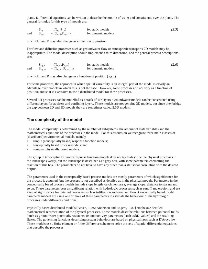
Increased complexity of a model only yields improved simulation up to a certain level. Given a certain amountof data, the addition of new state variables or parameters beyond a certain model complexity does not add to ourability to model the system, it only adds unaccounted uncertainty [Jørgensen, 1988]. Well-known laws ofdiminishing returns also apply to model development: 20% of the development time of the model is needed toreach 80% of the results, and an additional 80% of the development time improves the result by only 20% (seefigure 2.1).

Figure 2.1 The relation between model complexity, spatial and temporal resolution, knowledge gainedand costs of the model.

The above yields the conclusion that, although we are very much in search of the PERFECT model, in differentcases we need to apply different concepts and different models. It should be realised that choices that have to bemade for one of the characteristics of the model highly influence and are highly dependent on choicesconcerning the other characteristics of the model. In a good model design, there should be an equilibriumbetween the complexity introduced by the time dimension of the model and the complexity due to the spatialdimension and the process description. The use of a fully dynamic model with small time steps (minutes orhours) for the simulation of the runoff for a large catchment may prove an enormous waste of resources if thecatchment is described with one set of lumped parameters. This yields to a set of relations between spatialdistribution, temporal resolution and model complexity as shown in figure 2.1. Model designs that are locatedaround the diagonals of these figures are well balanced, models located off the diagonals may suffer from a toodetailed description of one or more of the characteristics and at the same time neglecting other characteristics.

The validation of the model is the process of evaluating the validity of the model concepts: that is evaluatinghow accurately the model describes real world processes and which processes are not accounted for. Validationinvolves the process of evaluating the significance for the original problem of the processes modelled and the

significance of the processes not modelled. Validation of the model is the process of evaluating whether thechoices made while defining the spatial scale, temporal scale and process descriptions are sufficiently robust toanalyse the processes that are considered relevant for the problem. Models may be validated if they do notviolate rules and physical laws, or if there is enough theoretical background to support the concepts. Validationcan be based on literature or on experiment. Once again, it is important to realize that there is no perfect model,and any model is only a simplification of reality. The question to be answered in the validation step is notwhether the model can be improved (any model can be improved), but whether the increase in costs forimproving (in terms of data, time, money and complexity) is balanced by an increase in benefits (accuracy andapplicability).

2.4 Integration of environmental models and GIS

2.4.1 Different levels of integration

Several authors recognize different levels of integration of GIS and models [Raper and Livingstone, 1993; Fedra,1993a; Nyerges, 1993; Van Deursen and Kwadijk, 1990, 1993]. The simplest approach is the use of separate GISand models, and exchange files. This approach requires at least five steps:• input of geographic distributed data through GIS;• export of GIS-data and conversion into the variables and parameters used in the model;• running the model;• importing the results of the model into GIS; and• analysis of the model-results and creating final maps and graphs.

Although this approach has the advantage of being straighforward and easy and cheap to develop, its use is notwithout serious disadvantages. Especially when running several models for a certain analysis, or using differentsets of input maps when analysing different scenarios, this ad hoc approach is cumbersome, not very flexible andpossibly error prone if it involves a significant amount of manual tasks.

An important extension for a fruitful marriage between GIS and models would be the establishment of acommon database structure that supports both GIS operations and model runs. In the case of dynamic modelling,this database should not only support the spatial distribution of geographic data, but in addition the storage oftemporal (and spatial) distributed input- and control-parameters. With such a database structure, the use of aspecific dynamic model can be invoked with one single command, and can be as simple (or complex) as the useof any other GIS-command. Any integration at this level, however, requires a sufficient open GIS architecturethat provides the interface and linkages necessary for tighter coupling [Fedra, 1993a]. This deeper level ofintegration would merge two approaches. The model becomes one of the analytical functions of the GIS, or theGIS becomes yet another option to generate, manipulate and display parameters, input and results of the model.

Because there are so many models it is difficult to choose which models should be incorporated into this mediumlevel integrated GIS - dynamic model environment. One could choose well-known models for different fields ofinterest, such as SHE [Abbott et al., 1986], TOPMODEL [Beven, 1985], MODFLOW [McDonald andHarbaugh, 1988] and ANSWERS [Beasley, 1977; De Roo, 1993] for hydrologic purposes, but a useful generalpurpose alternative would be to extend the GIS with a (limited) set of general tools that can be used to extractrelevant parameters and build environmental models to meet the user's requirements. This is an extension of theapproach used by Tomlin [1983] when he designed the Map Analysis Package. Instead of implementing alimited number of specific solutions for geographic problems, the GIS is a toolbox, with which an experienceduser can build solutions to solve many spatial problems. This high level approach yields a powerful tool forstoring, retrieving and analysing geographic data and allows one to explore how the processes of landscapes mayreact to human interference.

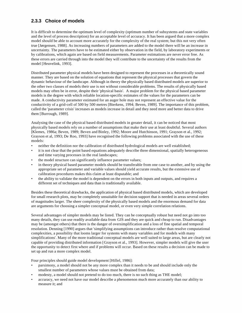
Figure 2.2 Levels of integration between GIS and (dynamic) models.

Although the distinction between the different levels of integration (figure 2.2) is vague, the levels can be rankedas:

Level 1Low level Standard GIS -> Manual exchange of files -> External model

::

Level 2MediumStandard GIS -> Automated exchange of files -> External model

::

Level 3High level Integrated GIS with modules for generic modelling

The low level linkage is characterised by the use of conversion programs and procedures, and data exchangebetween models and GIS using (in most cases ASCII) files. The medium level of linkage is characterised by anautomated and transparent procedure for exchanging data, mainly through the use of a common database, andallowing the model to address this database directly. In the high level of integration, the distinction betweenmodel and GIS becomes vague, and a dynamic model becomes just one of the applications that can beconstructed using the generic functionality of the GIS toolbox.

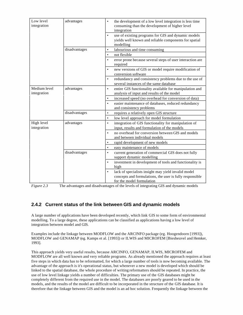
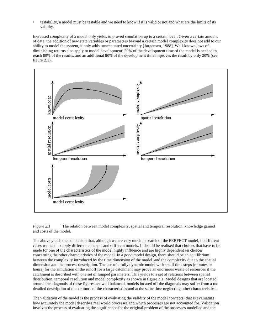
• the development of a low level integration is less timeconsuming than the development of higher levelintegration

advantages

• use of existing programs for GIS and dynamic modelsyields well known and reliable components for spatialmodelling

• labourious and time consuming• not flexible• error prone because several steps of user interaction are

required• new versions of GIS or model require modification of

conversion software

Low levelintegration

disadvantages

• redundancy and consistency problems due to the use ofseveral instances of the same database

• entire GIS functionality available for manipulation andanalysis of input and results of the model

• increased speed (no overhead for conversion of data)

advantages

• easier maintenance of databases, reduced redundancyand consistency problems

• requires a relatively open GIS structure

Medium levelintegration

disadvantages• low level approach for model formulation• integration of GIS functionality for manipulation of

input, results and formulation of the models• no overhead for conversion between GIS and models

and between individual models• rapid development of new models

advantages

• easy maintenance of models• current generation of commercial GIS does not fully

support dynamic modelling• investment in development of tools and functionality is

high

High levelintegration

disadvantages

• lack of specialists insight may yield invalid modelconcepts and formulations, the user is fully responsiblefor the model formulation

Figure 2.3 The advantages and disadvantages of the levels of integrating GIS and dynamic models

2.4.2 Current status of the link between GIS and dynamic models

A large number of applications have been developed recently, which link GIS to some form of environmentalmodelling. To a large degree, these applications can be classified as applications having a low level ofintegration between model and GIS.

Examples include the linkage between MODFLOW and the ARCINFO package (eg. Hoogendoorn [1993]),MODFLOW and GENAMAP (eg. Kamps et al. [1993]) or ILWIS and MICROFEM [Biesheuvel and Hemker,1993].

This approach yields very useful results, because ARCINFO, GENAMAP, ILWIS, MICROFEM andMODFLOW are all well known and very reliable programs. As already mentioned the approach requires at leastfive steps in which data has to be reformatted, for which a large number of tools is now becoming available. Theadvantage of the approach is it's operational status, but whenever a new model is developed which should belinked to the spatial database, the whole procedure of writing reformatters should be repeated. In practice, theuse of low level linkage yields a number of difficulties. The primary use of the GIS databases might becompletely different from the required use in the model. The databases are poorly geared to be used in themodels, and the results of the model are difficult to be incorporated in the structure of the GIS database. It istherefore that the linkage between GIS and the model is an ad hoc solution. Frequently the linkage between the

model and GIS is an once-only exercise, and the database used for the model is not updated along with the GISdatabase.

The medium level integration between the model and GIS is realized in approaches where the database of themodel is adapted so that it can be mapped directly on the GIS database. The required more open GIS databasestructure is not available in the above mentioned GIS systems, but several examples can be found in literature inwhich GRASS is linked to hydrological models such as ANSWERS (eg. Rewerts and Engel [1991]) andTOPMODEL (eg. Chairat and Delleur [1993], Romanowicz et al. [1993]). The authors of the latter paper definetheir implementation of TOPMODEL as a Water Information System (WIS), and remark that it can beconsidered one of several hydrologic application modules to become available in GRASS. They point out thatthere is a very important aspect of the integration of GIS and distributed models that must be emphasized.TOPMODEL has never been considered as a fixed model structure but rather as a set of modelling concepts thatcan be adapted and modified by the user. Thus, the general implementation of TOPMODEL allows for a user-interactive flexible adjustment of model structure depending on both predicted patterns of behaviour and theaims of the study.

The authors recognise three ways of integrating such a user-definition of model structure within GIS:• provide a set of variant structures as compiled routines that may be selected from a menu;• allow the user to provide an executable program segment with standardized inputs and outputs; or• provide a meta-language within which the user may define and modify the model structure.

Their WIS provides the capability to define models using the first two mentioned methods, and thus provide fora possibility to create a user defined model choosing from a number of predefined possibilities.

The same approach is followed for the design of the Modular Modelling System MMS [Leavesly et al., 1993].They argue that the increasing complexity and interdisciplinary nature of environmental problems require the useof modelling approaches from a broad range of science disciplines. They describe their approach as to selectivelycouple the most appropriate process algorithms to create an 'optimal' model for the desired application. Inaddition, their system allows for the coupling of a variety of GIS tools to characterize the topographic,hydrologic and biologic features of the watershed for use in a variety of lumped or distributed parametermodelling approaches.

This latter feature of the MSS represents another important field of linkage between GIS and environmentalmodels: the MSS is using the GIS data set to derive model parameters that can be used in external models. Formost environmental modelling projects, GIS is seen as a convenient and well-structured database for handlingthe large quantities of spatial data needed. Traditional GIS tools such as overlay and buffer are also important fordeveloping derivative data sets that serve as proxies for unavailable variables [Kemp, 1993a; Fedra, 1993c; Gaoet al., 1993; Moore et al., 1993; Maidment, 1993a]. Topographic features such as watersheds, ordered streamnetworks and topographic surface descriptors such as flow accumulation and flow length can be computed froman input DEM using functions available in current GIS. These features and surface descriptions are of primaryimportance for most surface hydrology models.

A somewhat different approach is advocated by Fedra [1993a]. He considers the problem of linking dynamicmodels and GIS as a part of the task of building spatial Decision Support Systems (DSS). Any efficient DSSshould allow a user to select criteria, and arbitrarily decide whether he wants to maximize or minimize them oruse them as a threshold for eliminating alternatives. However, the most important part of the DSS is thegeneration or design of the alternatives: if the set of alternatives to choose from is too small, and does not containsatisfactory (or 'optimal') solutions, the best ranking and selection methods cannot lead to satisfactory results. Adecision support system for spatial problems requires the capability to manipulate, display and analyse spatialdata and models. Alternatives need to be generated efficiently, analysed and compared. By excluding certainbasic GIS functions, such as data capture (ie. digitizing), and concentrating on the display and analysis of sets ofthematic maps and model output, GIS functionality can be embedded into a DSS framework. Most of theanalytical functionality is performed at the level of the model. Fedra argues that the distinction between modeland GIS becomes blurred, and meaningless if the model operates in terms of map overlays, and the analysis ofmap overlays is done by the model.

The previous sections described several characteristics of the levels of integration. Figure 2.3 summarises theadvantages and disadvantages of the recognised levels.

2.4.3 Required GIS functionality for high level linking with dynamic models

As can be concluded from the above, the high level integration is superior for a flexible formulation andimplementation of a large number of dynamic models. However, the high level integration of GIS and dynamicenvironmental modelling is hampered by a lack of some essential parts in the functionality of the GIS.

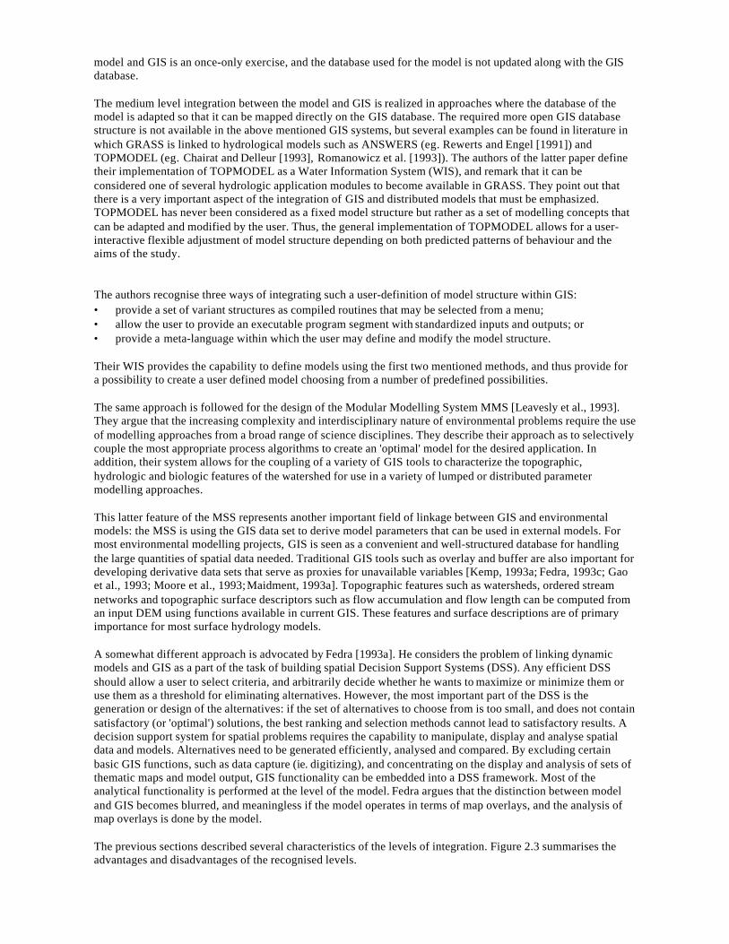
While dynamic environmental models deal with dynamically changing continuous data, current GIS manageonly static data. The current generation of GIS is not very well geared to implement these descriptions. Althoughsome GIS are capable of managing continuous data, the emphasis in most current GIS is on discrete objects.Since environmental models generally depend upon physical principles, the mathematics of these models is oftenin the form of differential equations that describe motion, diffusion, dispersion, transformation or some othermeaningful properties of continuous phenomena [Goodchild, 1993; Kemp, 1993b]. Although the currentgeneration GIS may be used to construct 1D process models, which are mostly vertical movement models, theylack functionality for the 2D and 3D description of lateral processes such as diffusion and dispersion processes(figure 2.4). The GIS should include all necessary primitives to allow for expression of these continuousphenomena. The level at which the individual primitives are defined should be closely related to the discipline ofenvironmental modelling, without sacrifying flexibility to create models from scratch.

Figure 2.4 Flows and state in a spatial dynamic system.

The data model used should be based on a functional distinction between continuous and discrete entities. Thesystem should eliminate the necessity to consider the implementation of the discretisation whenever possible.Moreover, for a high level integration of GIS and dynamic models, the systems should integrate support fordynamic variables, and allow for the use of time series describing changes in these variables over time.

The next chapters describe a prototype GIS that incorporates a large part of this preferred functionality.

3 MODELS AS AN INTEGRAL PART OF GIS

It does not seem to be productive to try to accomplish such simulations by intrinsic GIS functions; rather thesimulation model should be kept separate from the GIS and just use the GIS as a spatial data source.

(Maidment, 1993)

3.1 Introduction

This chapter deals with the high level integration of models in GIS. First the approach of using GIS scriptlanguages derived from Map Algebra and Cartographic Modelling techniques is discussed. It is argued that MapAlgebra can be considered as a normal (although very specialised) computer language. The deficiencies of MapAlgebra and Cartographic Modelling related to dynamic modelling are discussed. Before describing the criteriafor the development of a GIS script language that overcomes these disadvantages, this chapter discusses somegeneral aspects of dynamic models for environmental problems, and some aspects of computer languages anddata structures.

3.2 Map Algebra and concepts of implementing models in GIS

Map Algebra is a structured integrated set of primitives that can be used to create spatial models. Although thereare several versions of Map Algebra, all with different names, most of them seem to stem from one system, theMAP (Map Analysis Package) designed by Dana Tomlin [Tomlin, 1980]. Map Algebra consists of a set ofprimitive operators for map analysis, which can be linked into script files to perform complex analysis. As such,it is a computer language, which can be used to instruct the computer about the sequence of operations necessaryto perform a certain operation.

The linking of these Map Algebra commands into scripts used to instruct the computer how to obtain a certainresult is usually referred to as Cartographic Modelling. Tomlin describes Cartographic Modelling as an approachthat '... attempts to generalize and to standardize the use of geographic information systems. It does so bydecomposing the data processing tasks into elementary components, components that can then be recombinedwith ease and flexibility' [Tomlin, 1990]. The concept of combining the Map Algebra commands to form aCartographic Model script is similar to the combining of the keywords of a computer language to create aprogram. The commands available in the Map Algebra are the primitives of the operations that are possible withthe language. Operations in the Cartographic Model are either available as keywords in the Map Algebralanguage or can be easily constructed using the language. The major goal of the Cartographic Model script (andsimilar for computer programs) is to structure the problem in smaller steps and to instruct the computer in anunambiguous way what (GIS) commands should be performed to reach a certain result.

Several examples of the use of Cartographic Modelling are given by Burrough [1986] and Tomlin [1980, 1983,1990].

As has been observed above Cartographic Modelling languages can be considered as regular computerlanguages. The property that distinguishes Map Algebra from other computer languages is the fact that it is not ageneral purpose computer language, but one especially designed for spatial analysis. This means that manyoperations available in general purpose computer languages are not available in the Map Algebra languages,while commands that would take an enormous amount of coding in general purpose computer languages areavailable through one or only a few commands in the special purpose language.

In general, good computer languages will [Highman, 1967]:• allow you, somehow or other, to do anything you want to do which can be defined in the context of your

problem without reference to machine matters which lie outside this context;• make it easy to express the solution to your problem in terms which conform to the best practice in the

subject;

• allow such solutions to be expressed as compactly as possible without risking obscurity which oftenaccompanies compactness;

• be free of any constructs which can give rise to unintentional ambiguities;• permit the sort of ambiguity which is resolved dynamically, if the nature of the problem calls for it;• take over without change as much as possible of any well-formed descriptive language which is already

established in the field in which the problem originates;• allow for maintenance and easy apprehension: it should be possible to read and understand your own

programs and be able to change them without running too large risks of screwing up and it should bepossible to read other people's program and understand how they solve the problem; and

• allow for structuring the problem and evaluating and assessing the correctness of the approach.

GIS-languages developed for implementing dynamic models should be evaluated using the same set of criteria.Based on these criteria, the efficiency of a computer language can be considered. Efficiency can be measured fora number of aspects:• speed of execution;• space requirements;• efforts required to produce a program or system initially; and• efforts required to maintain the program.

Of these criteria, the first two are beyond the field of specialisation of geographers: they are highly linked tosoftware engineering and available hardware. In the early days of computing, both speed of execution and spacerequirements were of primary importance, and failing on one or both criteria could easily mean the failure of theproject. As the power of hardware increases, the importance of these hardware-related criteria decreases. Even ifan approach is too slow or too memory and disk space consuming by today's standards, in two years time theperformance of hardware will have doubled, and the critiques may very well be outdated.

The third and fourth criteria are much less related to hardware and software engineering, and have much morerelationship with the geographers and their field of expertise. Ultimately, the final test of the efficiency ofmodelling languages for dynamic models within GIS is whether geographers, hydrologists and environmentalistscan use the language without too much effort to produce and maintain models for their fields of interest.

Although quite a number of successful implementations of environmental models using Map Algebra andCartographic Modelling exist, the strong emphasis of the current versions is on the querying of a static database.From this static database, new data is derived which is added to the database, thus increasing the amount ofinformation in the database. The current versions of Map Algebra and Cartographic Modelling do not explicitlyallow for time dependent phenomena to be stored and analysed. As discussed in chapter 2, there is a seriousweakness when one tries to apply cartographic modelling techniques for modelling continuous phenomena anddynamic modelling fluxes of energy and substances through the landscape. Kemp [1993] discusses a strategy todeal with these issues. Her list can be considered as a list of requirements for the next generation of CartographicModelling languages:• allow expression and manipulation of variables and data about continuous phenomena in common symbolic

languages;• provide a syntax for incorporating primitive operations appropriate for environmental modelling with fields,

but are not yet available in GIS or common programming languages;• guide and enable the rapid development of a direct linkage between environmental models and any GIS;• the strategy should be capable of being incorporated into computer language implementations of

environmental models;• provide structures representing fields and incorporation of the concept of vector fields; and• eliminate the necessity to consider the form of the spatial discretization (the data model) whenever possible.

The first points are related to the issue of the level of the language. The last points are related to data structuresand data models. These issues are discussed in more detail in section 3.3.

3.3 Development of a dynamic cartographic modelling language

For the design of a computer language that can be used as a toolbox for dynamic modelling in GIS, three aspectsare important:• What is the level of abstraction of the language, is the level of abstraction appropriate for the problems that

you want to solve?− Are you capable of constructing the operators that are not part of the language from the primitives given

in the language, is the minimum number of primitives available sufficient for this field of applications?− Are the primitives generic enough to be used in many problems?− Is it possible to express the solution in terms that have any meaning in the field of practice, do the

primitives represent recognisable operations in the field of practice?• What is the data model used?

− What is the data structure for the spatial data?− Do the data types represent any recognisable phenomena in the field of practice?− What is the data structure for the temporal data?

• What are the control structures the language allows for?− Is there the necessity to create loops and iterations?− What control does the user needs over the sequence of calculations?− What control does the user has over the flow of the program (branching and conditional execution)?

Levels of abstraction; how to approach the problem

The first aspect deals with the level of abstraction. Abstraction is the process of identifying the important aspectsor properties of the phenomenon being modelled. Using a more abstract level, one can concentrate on therelevant aspects or properties of the phenomenon and ignore the irrelevant ones. What is relevant depends on thepurpose for which the abstraction is being designed [Ghezzi et al., 1982]. The level of abstraction determines theamount of commands that are necessary for a certain complex analysis. Increasing the level of abstraction meansthat one can more specifically address the problem. One needs fewer operators for solving the problem becauseeach operator can perform a more dedicated task. Increasing the level of abstraction results in a more specific setof operators, each having a more specialist purpose. However, to solve many different problems, one needs alarger set of operators to choose from. Increasing the level of abstraction means that the set to choose theoperators from is larger, but the number of operators required to perform a complex task decreases. This mightresult in a very high level language, for which the field of application becomes too narrow, or their command setbecomes too large.

Using languages with a low level of the abstraction, the programmer or user has to instruct the (GIS) system howto solve the problem. The user is responsible for the description of the structure of the problem and has to codethe algorithms necessary to solve the problem. The computer language is a means to define how to solve theproblem. Using higher levels of abstraction means that the focus is shifted from the algorithms of solving theproblem to the description and structuring of the problem to solve. This can be made clear by looking at theproblem of creating buffer zones around major rivers in a digital database. Using low level languages the userhas to tell the computer that he wants to create a map containing these buffer zones, and he has to code in aprogram how the computer should create these buffer zones. With a high level language the user only has to tellthe GIS that he wants buffer zones, while the system itself is responsible for the algorithms how to create thesebuffer zones.

The level of the language does not tell much about the capability of the language to perform a certain task. A lowlevel language, such as assembler, a general purpose language such as C and a high level language such as MapAlgebra are all capable of implementing the program to find the buffer zones around the major rivers. Theimplementation of a program to solve this problem would require approximately one to five lines of code in MapAlgebra. A general purpose language such as C would need a few hundred lines to implement this problem,while assembler could easily require tens of thousands of lines. Clearly the task is implemented most effectivelyin the highest level language. However, it is obvious that it is impossible to write a multi-user operating systemusing Map Algebra.

Data structures and data models;

raster or vector, that's not the question

The second aspect of the design of a computer language in general and a GIS-language for dynamic modelling isthe design of the data model. The architecture of the data management system determines the design of thedescriptive constructs used for data storage. As such, it is the fundamental mechanism for determining the natureof data representation as presented to application [Nyerges, 1993]. Computer languages are constructed arounddata types and data models. The language is the means by which the the data can be analysed and manipulated.

Clearly, for Map Algebra and Cartographic Modelling the data type under consideration is spatial data. There areonly a few primary data structures for storing spatial data. These have been long recognised and are responsiblefor the division in the GIS-world between vector and raster approaches. However, the breakdown of datastructures into raster and vector is not determined by the aims and purposes of GIS, but is a relic from the timesthat GIS was limited to a graphic map making environment. As GIS is used more and more for analyticalpurposes, the subdivision in raster and vector is not only too primitive, it may very well be completely obsoleteand superfluous.

Eventually, GIS-data will be stored in one form or the other, but for a functional support of the analyticalcapabilities of GIS, much more effort should go into a more sophisticated design of the data model. A moresophisticated design of the database should be based on the characteristics of the entities of interest. The entitiesare not related to the computer or the data structures geographic data should be stored in digitally, but relate tothe landscape and environment outside the computer. This simple fact means that we are not interested in theway the computer can store entities (the mechanics behind the database), but what we recognise as entities to bestored and manipulated (the concepts of the use of the information).

For dynamic modelling, the important entities may include information concerning water, soils, land use andpopulation. These entities can be stored using the well known geographic primitives such as points, lines andpolygons, or rasters, but by doing so, we neglect important information about the type of the entities. Addingadditional type information allows for a more intelligent use of the database and helps preventing errors andmistakes based on misinterpretation of the data. The mechanism of data storage to use can be classified as rasteror vector, but the type of the entity we want to store can hardly be described in terms of raster or vector. If weconsider the use of the entities for dynamic modelling purposes, a much more useful typing (although still veryprimitive) is in terms of continuous (physical) fields and classified objects.

Objects are those entities that may be counted, moved around, stacked, rotated, coloured labelled, cut, split,sliced, stuck together, viewed from different angles, shaded, inflated, shrunk, stored and retrieved. Objects arecharacterized by qualities of discrete identity, relative permanence of structure and attributes and their potentialto be manipulated [Couclelis, 1992]. Objects result from human action (building, constructing, allocating) orclassification.

A physical field is traditionally defined as an entity that is distributed over space and whose properties arefunctions of space coordinates and, in the case of dynamic fields, of time [Kemp, 1993]. Spatial continuousphenomena are best described by the concept of the field. Two types of fields may be recognised. Scalar fieldsare characterized by a function of position and, possibly, time, where each point is a scalar, while vector fieldsare characterized by a vector, i.e. both magnitude and direction. Scalar fields can be used to describe intensitiesand potentials, such as temperature, population density, precipitation etc. Vector fields are defined if not onlymagnitude but also direction is known. Vector fields can be used to represent (horizontal) fluxes and forces, suchas ground water movement and movement of air (wind and storms).

Objects are measured on nominal or ordinal scales (qualitative scales). Objects can, however, contain attributesthat come from interval and ratio scales. Fields are described in terms of ratio and interval scales (quantitativescales), and never as nominal and ordinal scales. Objects may be classified fields (such as soil maps where eachsoil type is an object, or topographic maps with polygons delineating areas (objects) with an elevation betweentwo values from the interval scale of elevation), or artifacts of human interference. Fields may be clustered toconstruct objects, which may be delineated because they embody a common set of values (soil maps,topographic map). Obviously, more mathematical operations are allowed with a quantitative scale than with aqualitative scale.

From the discussions on data models and data structures [Couclelis, 1992; Kemp, 1993; Goodchild, 1992;Burrough, 1992; Burrough and Frank, 1995], it is clear that the technical question of the most appropriate datastructure leads to the philosophical question of the most appropriate conceptualization of the geographic world.This question is stated by Couclelis [1992] as 'Is the geographic world a jig-saw puzzle of polygons, or a clubsandwich of data layers? '. This search for the most appropriate conceptualization is closely linked to thequestion whether the world surrounding us is made out of discrete and independent objects or made out ofnumerical fields that give rise to purely accidental clustering of some part of the field yielding a set of unstable,fleeting objects. The breakdown in camps in this discussion seems to follow the same delineations as can berecognised in the vector versus raster debate. People who want to conceptualize the world as identifiable objectsseem much more happy with the vector environment, while people who want to see the world as fields, or at bestas vague, weakly definable objects are defending the raster approach.

It should be realised however, that despite the philosophical questions whether 'reality' can be defined as crispobjects or as a spatio-temporal realisation of fields, scientists tend to use the most appropriate concept for thespecific question or purpose. The question is not whether the world consists of fields or objects, because quite anumber of geographic entities can be viewed both as an object or a field, depending on the application. Themajor question is whether we want to use a field-based or object-based view for a certain entity for the analysisof a certain problem. This implies that the main reason for storing geographic phenomena in the computer is notto represent the 'geographic reality' as accurate as possible at all cost, but to store geographic phenomena asaccurate as possible and required for a certain purpose. It is the purpose why we store a certain geographic entitythat should drive the choice between object and field representation. The data model is always a simplification ofreality, and the quality of the choice for a specific data model is determined by the phenomenon studied and thespecific questions to be answered. There will always be a need for the description of reality as both a crisp objectrelated description as for the field description. The main purpose of the discussion is not to define one datastructure that can store all geographic entities and possible views, but to allow for the appropriate data type to bechosen for a specific geographic phenomenon or entity.

If we consider the Cartographic Modelling and Map Algebra as defined by Tomlin and Berry [1979], theconclusion can be drawn that Map Algebra is stronger related to the object data models than to the field models.A large number of operators on objects are defined, while the analysis of spatial fields is much weakerdeveloped. Constructing operators using the concepts of vector fields are virtually impossible with the standardMap Algebra. Moreover, Map Algebra is designed to work with time-independent databases: the variables storedin the database do not change as a function of time. Cartographic Modelling can be used for dynamic modelling,but the burden of keeping track of time dependent variables, inputs and result are totally on the shoulder of theuser.

As discussed, the choice of describing the geographic entities using more meaningful type definitions such asfields or objects (conceptual types) is a much more fundamental one than the question whether the data shouldbe stored as vector or raster (technical implementation structures). This choice defines the measurement scale ofthe entity stored, and thus the choice between a field representation and an object representation defines veryclearly which operations are permitted on the entity. This has much more important implications than thequestion whether these operations are implemented in the specific data structure.

In both vector and raster systems, we can implement operations for counting, adding, combination and findingthe shortest route between hospitals and accidents. However, operations such as the addition two overlays thatcontain soil types (= objects with a nominal scale) will yield unwanted results, no matter whether implementedin a raster or vector domain.

In general, we can see that implications of the choice between the qualitative scales (nominal and ordinal scales)and the quantitative scales (ratio and interval scales) is a very important one. Although technically veryachievable, entities on a nominal scale do not support any mathematical operations, whereas fields allow for anextensive set of mathematical operations. It is not the (technical) data structure that determines if the operation ispermitted, but the data type that is responsible for the set of operations.

Strong type checking versus loose type checking

There is always the discussion on how strictly to apply data typing. One standpoint in the discussion is that strictdata typing is a restriction on the possible combinations of operators that a user may want to perform. Theargument is that the user may have a very specific question in which he wants to perform an operation on a type

that would in theory not allow such an operation. Examples are that there might be a complex analysis in whichit may be useful to take the square root of the entities that are in a soil map. The soil map may be stored as alarge number of positive integer values, each representing one category in the soil map. Taking a square rootfrom these positive integer values is a completely valid operation and the language should not prohibit this kindof analysis.

The opposite attitude is that operations never yield valid results if the data used for the operation is notappropriate for this operation. There may be a single analysis in which a square root of a soil type yields a resultthat can be interpreted, but in general this operation is nonsense. Therefore, these mathematical functions shouldnot work on the soil type map. If the necessity exists for an operation to be performed on an inappropriate datatype, it simply means that the set of commands is not complete, and a complementary command should bedefined, capable of performing the wanted operation in the proper type domain.

Adding strong type information to data also allows for the implementation of polymorphic functions. A certainfunction or operation may have different functionality based on different types of input. This can be explained byanalysing resampling and interpolation operators. If no data type information is supplied, the user has to decidewhich method of interpolation and resampling should be used, and most GIS offer the choice between a nearestneighbour and a (bi-)linear interpolation. However, if the data supplied to the operator is classified data, theoption of using a (bi-)linear interpolation would not yield any useful results, while if the data supplied is from acontinuous scale, the bi-linear interpolation would yield highly superior results over the nearest neighbourapproach. Although most GIS provide the user in this case with an option to choose, if the type of the data isknown, the operation can determine the optimal approach without consulting the user. As a result of a soundtyping and type checking mechanism, more intelligence can be added to the system.

Although the discussion is an ongoing one, it has long been recognised that there is some substantial motivationfor strong data typing. Summarising, the following list can be given:• types help to understand and organise our ideas about entities;• a type scheme helps to see and discuss unique properties of specific types;• types help to detect errors; and• types allow for polymorphic behaviour of functions and operators.

The division of data in field (or continuous) data and object (or classified) data is hardly sufficient for allpurposes. We should be careful to expect the fact that we add type information to geographical data will preventall errors. The fact that an operation is permitted on a certain set of geographic information does not guaranteethe meaning and sense of the operation. However, adding type information allows for mechanisms to avoid thoseoperations that will absolutely make no sense. The classification in fields and objects can be considered as theprimitives of a more functional typology of geographic information. The field versus object classification ofgeographic data may prove to be a much more stable root to support a more intelligent and robust tree of datastructures than the vector versus raster classification.

Control structures in computer languages

Most of the conventional computer languages offer a set of constructs for creating loops and explicitconstruction of iterative procedures. Loops are those constructs that allow for repeatedly execution of a (set of)statements. Although most conventional computer languages allow for loops, several languages may be listedthat do not include these constructs. Within the framework of dynamic spatial modelling, these constructs areuseful to a limited set of purposes:• iteration over space;• iteration over time; and• iteration to increase accuracy of the calculations.

The explicit iteration over space is essential if the entity addressed by the operators is only part of the totalspatial coverage of the database layer. Operators that address individual cells in raster maps need to be executedrepeatedly to be applied to the total database layer. Operators that address entire maps do not have to be executediteratively, although their internal implementation might include several loops.

If the operator addresses individual cells in the raster database layer, the instruction of multiplying cell values by100 (to yield values in centimetres instead of metres) could be implemented with

/* operator addresses individual cells */for (row = 0; row <= LastRow; row++) for (col = 0; col <= LastCol; col++) NewMap[row][col] = OldMap[row][col] * 100;

The user is responsible for providing the loop statements to make sure every cell in the database layer isaddressed. However, if the operator addresses all cells in the database layer, the explicit construction of thespatial loop is no longer necessary, and the same result could be achieved by

/* operator addresses entire database layer */NewMap = OldMap * 100;

The second approach yields a language that does not require explicit spatial loop constructs. The statement in thesecond example does not make any assumptions on the database structure, and could be used to addresscontinuous fields stored in any of the database structures (raster, vector, TIN or any other). It eliminates thenecessity to consider the form of spatial discretization, whereas the statements given in the first approach onlyapply to raster databases.

The second use for loop constructs in dynamic spatial modelling languages is to create iterations through time.The same principles as described above can be applied to iteration through the time domain. These iterationsmay be implemented with explicit loops or may be implicit in the language. The explicit definition of time loopswould require statements such as

/* explicit iterations through time */InitiateModel;for(time = BeginTime; time <= EndTime, time++) ExecuteModel;

while the implicit definition requires statements such as

/* implicit definition of the iteration through time */timer BeginTime, EndTime, TimeStep;

initial InitiateModel;

dynamic ExecuteModel;

Again, the second approach does not require the use of explicit loop statements.

The third use of loops and repeatedly execution of statements is for implementing numerical methods for solvingcertain problems. Most of these problems cannot be solved analytically, and solutions are obtained by obtainingan approximate trail solution and repeatedly improving on the solution until some predetermined convergencecriterion is satisfied. These techniques are used to solve many problems related to dynamic spatial modelling.Examples are solutions for ordinary and partial differential equations (used to describe mass movement as afunction of space and time) and root finding procedures. It is important to realise however, that the loops used inthese techniques are not part of the problem definition (they do not describe what should be modelled), but partof the numerical techniques to solve the problem (they describe how the problem should be solved). Similar tothe principle described above, the iteration for solving the problem can be explicit, where it is the task of the userto provide the control statements, or implicit, where the iteration is inherent to the problem formulation.

Explicit formulation the iterations for root finding requires statements such as

/* explicit formulation of loops for increased accuracy */do { find_improved_solution(....); } while (accuracy > converge_criterion);

and implicit formulation only requires the definition of the problem

/* implicit algorithm for solving root finding problems with required accuracy */find_root(...., convergence_criterium);

The above yields the conclusion that although iterative constructs for repeatedly executing statements seemindispensable for general purpose languages, when considering languages for dynamic spatial modelling theirneed is less essential. Most of the traditional use of these constructs appears related with data implementationissues and numerical number crunching techniques. Although loops and iterations are crucial for theimplementation of the language, they do not have to be an essential part of the dynamic modelling language.

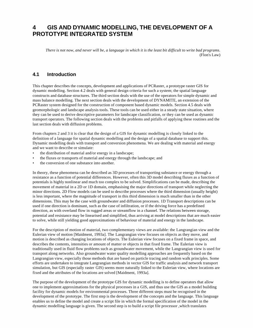
4 GIS AND DYNAMIC MODELLING, THE DEVELOPMENT OF APROTOTYPE INTEGRATED SYSTEM

There is not now, and never will be, a language in which it is the least bit difficult to write bad programs.(Flon's Law)

4.1 Introduction

This chapter describes the concepts, development and applications of PCRaster, a prototype raster GIS fordynamic modelling. Section 4.2 deals with general design criteria for such a system; the spatial languageconstructs and database structures. The third section deals with the use of the operators for simple dynamic andmass balance modelling. The next section deals with the development of DYNAMITE, an extension of thePCRaster system designed for the construction of component based dynamic models. Section 4.5 deals withgeomorphologic and landscape analysis tools. These tools can be used either in a steady state situation, wherethey can be used to derive descriptive parameters for landscape classification, or they can be used as dynamictransport operators. The following section deals with the problems and pitfalls of applying these routines and thelast section deals with diffusion problems.

From chapters 2 and 3 it is clear that the design of a GIS for dynamic modelling is closely linked to thedefinition of a language for spatial dynamic modelling and the design of a spatial database to support this.Dynamic modelling deals with transport and conversion phenomena. We are dealing with material and energyand we want to describe or simulate:• the distribution of material and/or energy in a landscape;• the fluxes or transports of material and energy through the landscape; and• the conversion of one substance into another.

In theory, these phenomena can be described as 3D processes of transporting substance or energy through aresistance as a function of potential differences. However, often this 3D model describing fluxes as a function ofpotentials is highly nonlinear and much too complex to be solved. Simplifications can be made, describing themovement of material in a 2D or 1D domain, emphasising the major directions of transport while neglecting theminor directions. 2D Flow models can be used to describe processes where the third dimension (usually height)is less important, where the magnitude of transport in this third dimension is much smaller than in the otherdimensions. This may be the case with groundwater and diffusion processes. 1D Transport descriptions can beused if one direction is dominant, such as the case of infiltration, or if the driving force has a predefineddirection, as with overland flow in rugged areas or streamflow in a channel. The relations between storage,potential and resistance may be linearised and simplified, thus arriving at model descriptions that are much easierto solve, while still yielding good approximations of behaviour of material and energy in the landscape.

For the description of motion of material, two complementary views are available: the Langrangian view and theEulerian view of motion [Maidment, 1993a]. The Langrangian view focuses on objects as they move, andmotion is described as changing locations of objects. The Eulerian view focuses on a fixed frame in space, anddescribes the contents, intensities or amount of matter or objects in that fixed frame. The Eulerian view istraditionally used in fluid flow problems such as groundwater movement, while the Langrangian view is used fortransport along networks. Also groundwater water quality modelling approaches are frequently based on theLangrangian view, especially those methods that are based on particle tracing and random walk principles. Someefforts are undertaken to integrate Langrangian methods in vector GIS for traffic analysis and network transportsimulation, but GIS (especially raster GIS) seems more naturally linked to the Eulerian view, where locations arefixed and the attributes of the locations are solved [Maidment, 1993a].

The purpose of the development of the prototype GIS for dynamic modelling is to define operators that allowone to implement approximations for the physical processes in a GIS, and thus use the GIS as a model buildingfacility for dynamic models for environmental processes. Three different steps must be recognised in thedevelopment of the prototype. The first step is the development of the concepts and the language. This languageenables us to define the model and create a script file in which the formal specification of the model in thedynamic modelling language is given. The second step is to build a script file processor ,which translates

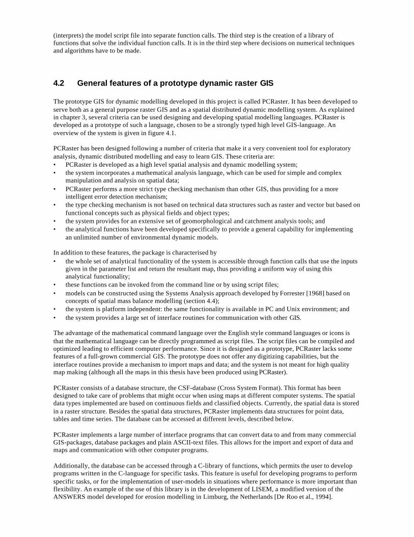
(interprets) the model script file into separate function calls. The third step is the creation of a library offunctions that solve the individual function calls. It is in the third step where decisions on numerical techniquesand algorithms have to be made.

4.2 General features of a prototype dynamic raster GIS

The prototype GIS for dynamic modelling developed in this project is called PCRaster. It has been developed toserve both as a general purpose raster GIS and as a spatial distributed dynamic modelling system. As explainedin chapter 3, several criteria can be used designing and developing spatial modelling languages. PCRaster isdeveloped as a prototype of such a language, chosen to be a strongly typed high level GIS-language. Anoverview of the system is given in figure 4.1.

PCRaster has been designed following a number of criteria that make it a very convenient tool for exploratoryanalysis, dynamic distributed modelling and easy to learn GIS. These criteria are:• PCRaster is developed as a high level spatial analysis and dynamic modelling system;• the system incorporates a mathematical analysis language, which can be used for simple and complex

manipulation and analysis on spatial data;• PCRaster performs a more strict type checking mechanism than other GIS, thus providing for a more

intelligent error detection mechanism;• the type checking mechanism is not based on technical data structures such as raster and vector but based on

functional concepts such as physical fields and object types;• the system provides for an extensive set of geomorphological and catchment analysis tools; and• the analytical functions have been developed specifically to provide a general capability for implementing

an unlimited number of environmental dynamic models.

In addition to these features, the package is characterised by• the whole set of analytical functionality of the system is accessible through function calls that use the inputs

given in the parameter list and return the resultant map, thus providing a uniform way of using thisanalytical functionality;

• these functions can be invoked from the command line or by using script files;• models can be constructed using the Systems Analysis approach developed by Forrester [1968] based on

concepts of spatial mass balance modelling (section 4.4);• the system is platform independent: the same functionality is available in PC and Unix environment; and• the system provides a large set of interface routines for communication with other GIS.

The advantage of the mathematical command language over the English style command languages or icons isthat the mathematical language can be directly programmed as script files. The script files can be compiled andoptimized leading to efficient computer performance. Since it is designed as a prototype, PCRaster lacks somefeatures of a full-grown commercial GIS. The prototype does not offer any digitizing capabilities, but theinterface routines provide a mechanism to import maps and data; and the system is not meant for high qualitymap making (although all the maps in this thesis have been produced using PCRaster).

PCRaster consists of a database structure, the CSF-database (Cross System Format). This format has beendesigned to take care of problems that might occur when using maps at different computer systems. The spatialdata types implemented are based on continuous fields and classified objects. Currently, the spatial data is storedin a raster structure. Besides the spatial data structures, PCRaster implements data structures for point data,tables and time series. The database can be accessed at different levels, described below.

PCRaster implements a large number of interface programs that can convert data to and from many commercialGIS-packages, database packages and plain ASCII-text files. This allows for the import and export of data andmaps and communication with other computer programs.

Additionally, the database can be accessed through a C-library of functions, which permits the user to developprograms written in the C-language for specific tasks. This feature is useful for developing programs to performspecific tasks, or for the implementation of user-models in situations where performance is more important thanflexibility. An example of the use of this library is in the development of LISEM, a modified version of theANSWERS model developed for erosion modelling in Limburg, the Netherlands [De Roo et al., 1994].

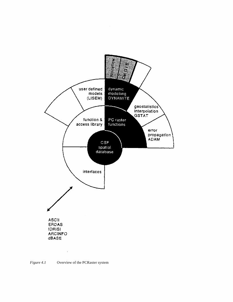
Figure 4.1 Overview of the PCRaster system

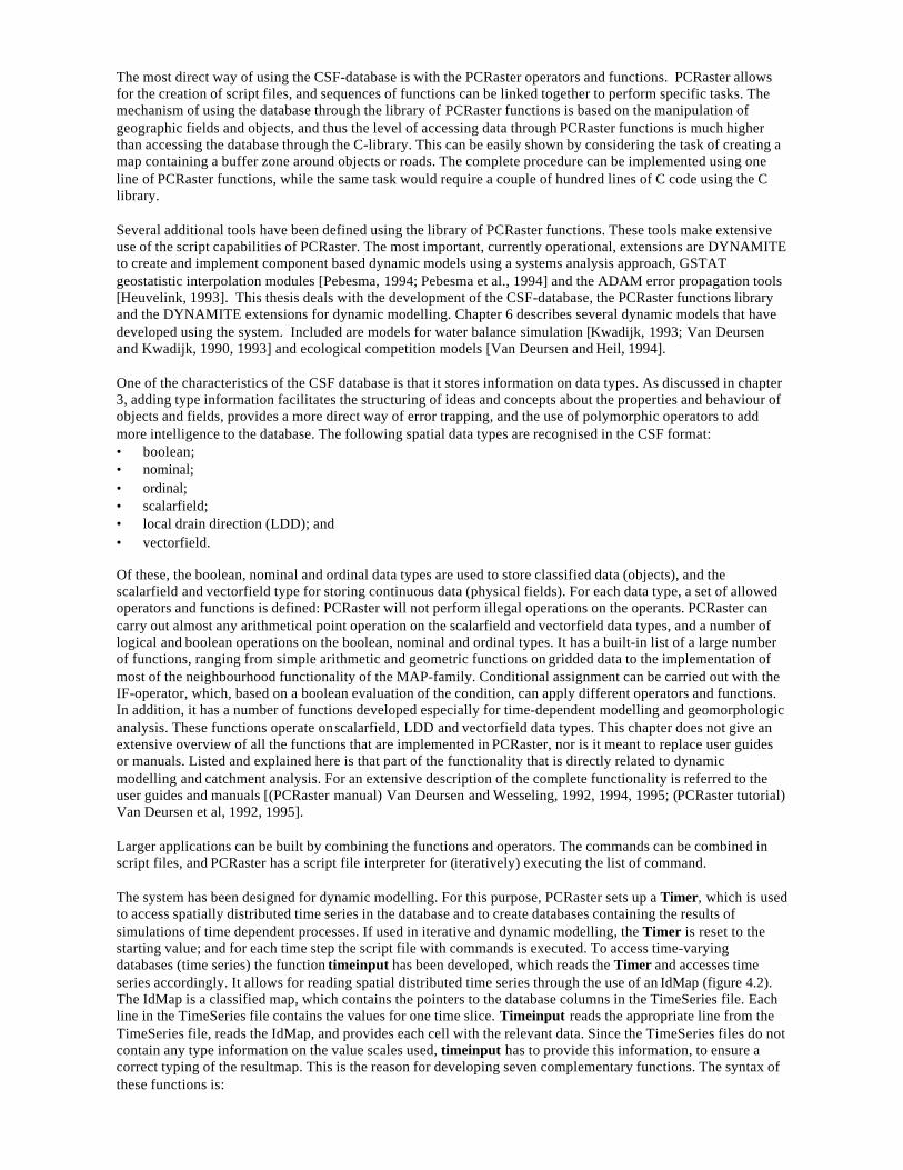
The most direct way of using the CSF-database is with the PCRaster operators and functions. PCRaster allowsfor the creation of script files, and sequences of functions can be linked together to perform specific tasks. Themechanism of using the database through the library of PCRaster functions is based on the manipulation ofgeographic fields and objects, and thus the level of accessing data through PCRaster functions is much higherthan accessing the database through the C-library. This can be easily shown by considering the task of creating amap containing a buffer zone around objects or roads. The complete procedure can be implemented using oneline of PCRaster functions, while the same task would require a couple of hundred lines of C code using the Clibrary.

Several additional tools have been defined using the library of PCRaster functions. These tools make extensiveuse of the script capabilities of PCRaster. The most important, currently operational, extensions are DYNAMITEto create and implement component based dynamic models using a systems analysis approach, GSTATgeostatistic interpolation modules [Pebesma, 1994; Pebesma et al., 1994] and the ADAM error propagation tools[Heuvelink, 1993]. This thesis deals with the development of the CSF-database, the PCRaster functions libraryand the DYNAMITE extensions for dynamic modelling. Chapter 6 describes several dynamic models that havedeveloped using the system. Included are models for water balance simulation [Kwadijk, 1993; Van Deursenand Kwadijk, 1990, 1993] and ecological competition models [Van Deursen and Heil, 1994].

One of the characteristics of the CSF database is that it stores information on data types. As discussed in chapter3, adding type information facilitates the structuring of ideas and concepts about the properties and behaviour ofobjects and fields, provides a more direct way of error trapping, and the use of polymorphic operators to addmore intelligence to the database. The following spatial data types are recognised in the CSF format:• boolean;• nominal;• ordinal;• scalarfield;• local drain direction (LDD); and• vectorfield.

Of these, the boolean, nominal and ordinal data types are used to store classified data (objects), and thescalarfield and vectorfield type for storing continuous data (physical fields). For each data type, a set of allowedoperators and functions is defined: PCRaster will not perform illegal operations on the operants. PCRaster cancarry out almost any arithmetical point operation on the scalarfield and vectorfield data types, and a number oflogical and boolean operations on the boolean, nominal and ordinal types. It has a built-in list of a large numberof functions, ranging from simple arithmetic and geometric functions on gridded data to the implementation ofmost of the neighbourhood functionality of the MAP-family. Conditional assignment can be carried out with theIF-operator, which, based on a boolean evaluation of the condition, can apply different operators and functions.In addition, it has a number of functions developed especially for time-dependent modelling and geomorphologicanalysis. These functions operate on scalarfield, LDD and vectorfield data types. This chapter does not give anextensive overview of all the functions that are implemented in PCRaster, nor is it meant to replace user guidesor manuals. Listed and explained here is that part of the functionality that is directly related to dynamicmodelling and catchment analysis. For an extensive description of the complete functionality is referred to theuser guides and manuals [(PCRaster manual) Van Deursen and Wesseling, 1992, 1994, 1995; (PCRaster tutorial)Van Deursen et al, 1992, 1995].

Larger applications can be built by combining the functions and operators. The commands can be combined inscript files, and PCRaster has a script file interpreter for (iteratively) executing the list of command.

The system has been designed for dynamic modelling. For this purpose, PCRaster sets up a Timer, which is usedto access spatially distributed time series in the database and to create databases containing the results ofsimulations of time dependent processes. If used in iterative and dynamic modelling, the Timer is reset to thestarting value; and for each time step the script file with commands is executed. To access time-varyingdatabases (time series) the function timeinput has been developed, which reads the Timer and accesses timeseries accordingly. It allows for reading spatial distributed time series through the use of an IdMap (figure 4.2).The IdMap is a classified map, which contains the pointers to the database columns in the TimeSeries file. Eachline in the TimeSeries file contains the values for one time slice. Timeinput reads the appropriate line from theTimeSeries file, reads the IdMap, and provides each cell with the relevant data. Since the TimeSeries files do notcontain any type information on the value scales used, timeinput has to provide this information, to ensure acorrect typing of the resultmap. This is the reason for developing seven complementary functions. The syntax ofthese functions is:

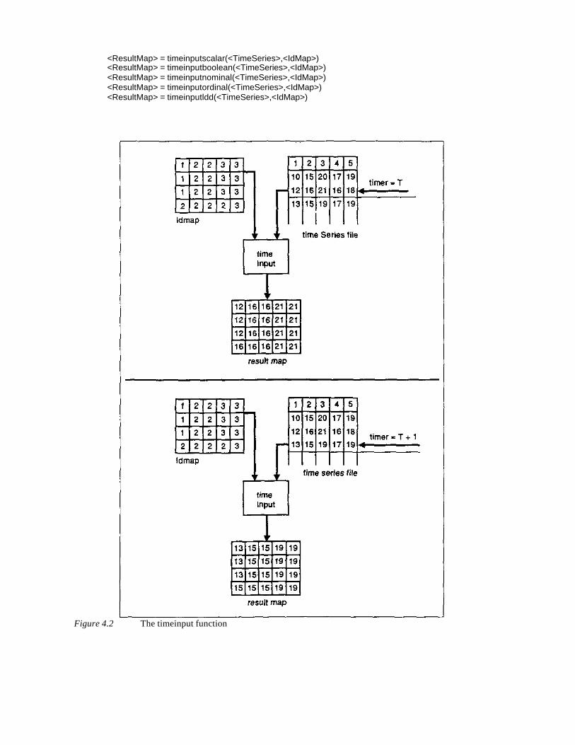
<ResultMap> = timeinputscalar(<TimeSeries>,<IdMap>)<ResultMap> = timeinputboolean(<TimeSeries>,<IdMap>)<ResultMap> = timeinputnominal(<TimeSeries>,<IdMap>)<ResultMap> = timeinputordinal(<TimeSeries>,<IdMap>)<ResultMap> = timeinputldd(<TimeSeries>,<IdMap>)

Figure 4.2 The timeinput function

To write results of the models to time series, the report keyword is used. Two functions are defined to store thevalue at a certain location (function timeoutput) or statistics such as the mean, standard deviation, minimum andmaximum values of a dynamic map (function summary). The syntax of these functions is:

report <TimeSeries> = timeoutput(<IdMap>,<Expression>)report <TimeSeries> = summary(<Expression>)

For the creation of a dynamic model, several sections in the script file may be recognised. The first section is thebinding section, in which symbol names of the model are bound to external files (maps, tables etc.). Its mainpurpose is to separate external names, such as files, from model symbols. The areamap section is the definitionof the modelling area and modelling resolution. All input maps are masked by this map and resampled to itsresolution. The next section is the timer section. The timer section describes the start time, time slice and endtime for the model. The next section is the initial in which assignments to maps are made before the dynamicexpressions are executed. The initial section is used to set initial values for the dynamic maps. Next is thedynamic section, describing the dynamic behaviour of the model. The loops necessary for iterative modelling arecontrolled by the system and are not the responsibility of the user. An example of a script file for dynamicmodelling is given in the next section.

4.3 Simple one dimensional and mass balance modelling

The application of the GIS for dynamic modelling is best described using an example. Consider theimplementation of a simple method for computing excess rainfall and abstractions from storm rainfall.Abstractions include interception of precipitation on vegetation above the ground, depression storage on theground surface and infiltration of water into the soil. The method described is developed by the U.S. SoilConservation Service (SCS) [1972] and is known as the Curve Number (CN-) method. The method is based onthe concept of limited recharge capacity of a basin, related to antecedent moisture conditions and physicalcharacteristics of the basin. For a storm as a whole, the depth of excess precipitation (Pe) is always less than orequal to the depth of precipitation P. There is some amount of rainfall Ia (initial abstraction before ponding) forwhich no runoff will occur, so the potential runoff is P-Ia. After runoff begins, an additional depth of water isretained in the basin, which is less than or equal to some potential maximum retention S. The assumed relationbetween precipitation, potential maximum retention, initial retention (Ia) and additional depth of water retainedin the catchment as:

S)+Ia-(P)Ia-(P

=Pe2

(4.1)

withPe = excess precipitation or direct runoff (inches)P = precipitation (inches)Ia = initial abstraction before ponding (inches)S = potential maximum retention (inches)

By studying the results of many small experimental catchments, an empirical relation has been developed:

0.2S=Ia (4.2)

Combining equation 4.1 with equation 4.2 gives:

0.8S)+(P)0.2S-(P

=Pe2

(4.3)

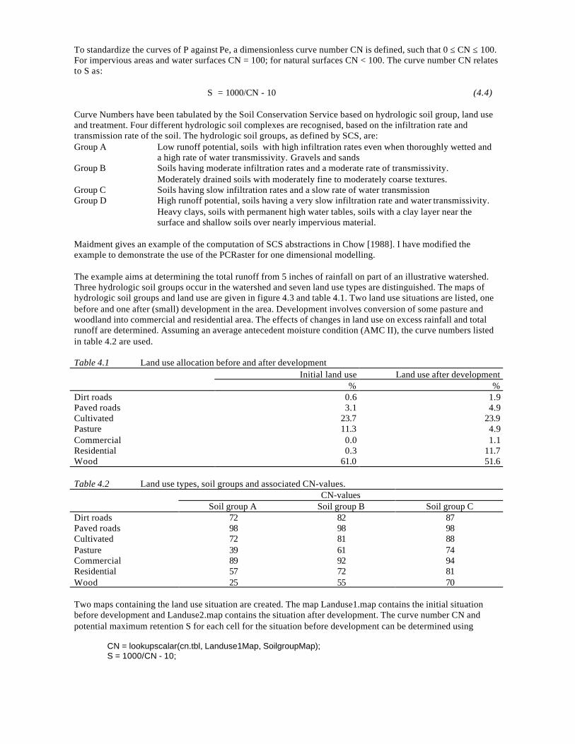
To standardize the curves of P against Pe, a dimensionless curve number CN is defined, such that 0 ≤ CN ≤ 100.For impervious areas and water surfaces CN = 100; for natural surfaces CN < 100. The curve number CN relatesto S as:

S = 1000/CN - 10 (4.4)

Curve Numbers have been tabulated by the Soil Conservation Service based on hydrologic soil group, land useand treatment. Four different hydrologic soil complexes are recognised, based on the infiltration rate andtransmission rate of the soil. The hydrologic soil groups, as defined by SCS, are:Group A Low runoff potential, soils with high infiltration rates even when thoroughly wetted and

a high rate of water transmissivity. Gravels and sandsGroup B Soils having moderate infiltration rates and a moderate rate of transmissivity.

Moderately drained soils with moderately fine to moderately coarse textures.Group C Soils having slow infiltration rates and a slow rate of water transmissionGroup D High runoff potential, soils having a very slow infiltration rate and water transmissivity.

Heavy clays, soils with permanent high water tables, soils with a clay layer near thesurface and shallow soils over nearly impervious material.

Maidment gives an example of the computation of SCS abstractions in Chow [1988]. I have modified theexample to demonstrate the use of the PCRaster for one dimensional modelling.

The example aims at determining the total runoff from 5 inches of rainfall on part of an illustrative watershed.Three hydrologic soil groups occur in the watershed and seven land use types are distinguished. The maps ofhydrologic soil groups and land use are given in figure 4.3 and table 4.1. Two land use situations are listed, onebefore and one after (small) development in the area. Development involves conversion of some pasture andwoodland into commercial and residential area. The effects of changes in land use on excess rainfall and totalrunoff are determined. Assuming an average antecedent moisture condition (AMC II), the curve numbers listedin table 4.2 are used.

Table 4.1 Land use allocation before and after developmentInitial land use Land use after development

% %Dirt roads 0.6 1.9Paved roads 3.1 4.9Cultivated 23.7 23.9Pasture 11.3 4.9Commercial 0.0 1.1Residential 0.3 11.7Wood 61.0 51.6

Table 4.2 Land use types, soil groups and associated CN-values.CN-values

Soil group A Soil group B Soil group CDirt roads 72 82 87Paved roads 98 98 98Cultivated 72 81 88Pasture 39 61 74Commercial 89 92 94Residential 57 72 81Wood 25 55 70

Two maps containing the land use situation are created. The map Landuse1.map contains the initial situationbefore development and Landuse2.map contains the situation after development. The curve number CN andpotential maximum retention S for each cell for the situation before development can be determined using

CN = lookupscalar(cn.tbl, Landuse1Map, SoilgroupMap);S = 1000/CN - 10;

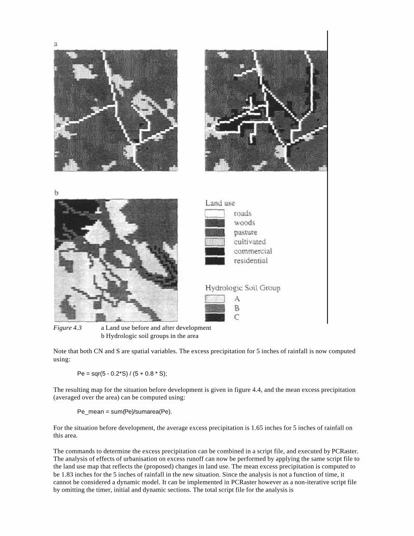
Figure 4.3 a Land use before and after developmentb Hydrologic soil groups in the area

Note that both CN and S are spatial variables. The excess precipitation for 5 inches of rainfall is now computedusing:

Pe = sqr(5 - 0.2*S) / (5 + 0.8 * S);

The resulting map for the situation before development is given in figure 4.4, and the mean excess precipitation(averaged over the area) can be computed using:

Pe_mean = sum(Pe)/sumarea(Pe).

For the situation before development, the average excess precipitation is 1.65 inches for 5 inches of rainfall onthis area.

The commands to determine the excess precipitation can be combined in a script file, and executed by PCRaster.The analysis of effects of urbanisation on excess runoff can now be performed by applying the same script file tothe land use map that reflects the (proposed) changes in land use. The mean excess precipitation is computed tobe 1.83 inches for the 5 inches of rainfall in the new situation. Since the analysis is not a function of time, itcannot be considered a dynamic model. It can be implemented in PCRaster however as a non-iterative script fileby omitting the timer, initial and dynamic sections. The total script file for the analysis is

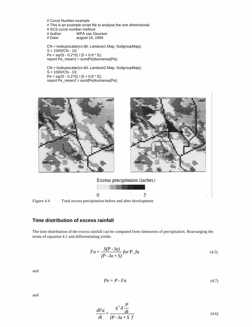
# Curve Number example# This is an example script file to analyse the one dimensional# SCS curve number method# Author: WPA van Deursen# Date: august 16, 1994

CN = lookupscalar(cn.tbl, Landuse1.Map, SoilgroupMap);S = 1000/CN - 10;Pe = sqr(5 - 0.2*S) / (5 + 0.8 * S);report Pe_mean1 = sum(Pe)/sumarea(Pe);

CN = lookupscalar(cn.tbl, Landuse2.Map, SoilgroupMap);S = 1000/CN - 10;Pe = sqr(5 - 0.2*S) / (5 + 0.8 * S);report Pe_mean2 = sum(Pe)/sumarea(Pe);

Figure 4.4 Total excess precipitation before and after development

Time distribution of excess rainfall

The time distribution of the excess rainfall can be computed from timeseries of precipitation. Rearranging theterms of equation 4.1 and differentiating yields:

and

and

IaPforS)+Ia-(P

Ia)-S(P=Fa _ (4.5)

)S+Ia-(PdtP

dS=

dtdFa

2

2

(4.6)

Fa-P=Pe (4.7)

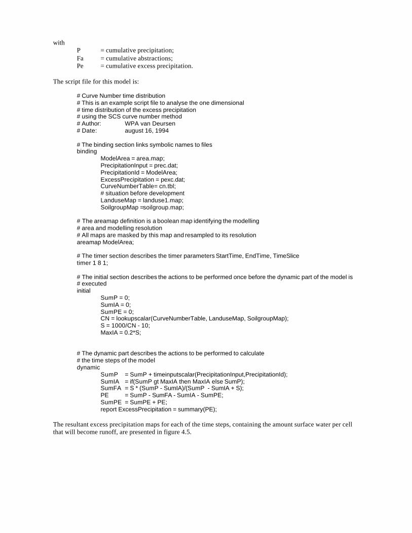
withP = cumulative precipitation;Fa = cumulative abstractions;Pe = cumulative excess precipitation.

The script file for this model is:

# Curve Number time distribution# This is an example script file to analyse the one dimensional# time distribution of the excess precipitation# using the SCS curve number method# Author: WPA van Deursen# Date: august 16, 1994

# The binding section links symbolic names to filesbinding

ModelArea = area.map;PrecipitationInput = prec.dat;PrecipitationId = ModelArea;ExcessPrecipitation = pexc.dat;CurveNumberTable= cn.tbl;# situation before developmentLanduseMap = landuse1.map;SoilgroupMap =soilgroup.map;

# The areamap definition is a boolean map identifying the modelling# area and modelling resolution# All maps are masked by this map and resampled to its resolutionareamap ModelArea;

# The timer section describes the timer parameters StartTime, EndTime, TimeSlicetimer 1 8 1;

# The initial section describes the actions to be performed once before the dynamic part of the model is# executedinitial

SumP = 0;SumIA = 0;SumPE = 0;CN = lookupscalar(CurveNumberTable, LanduseMap, SoilgroupMap);S = 1000/CN - 10;MaxIA = 0.2*S;

# The dynamic part describes the actions to be performed to calculate# the time steps of the modeldynamic

SumP = SumP + timeinputscalar(PrecipitationInput,PrecipitationId);SumIA = if(SumP gt MaxIA then MaxIA else SumP);SumFA = S * (SumP - SumIA)/(SumP - SumIA + S);PE = SumP - SumFA - SumIA - SumPE;SumPE = SumPE + PE;report ExcessPrecipitation = summary(PE);

The resultant excess precipitation maps for each of the time steps, containing the amount surface water per cellthat will become runoff, are presented in figure 4.5.

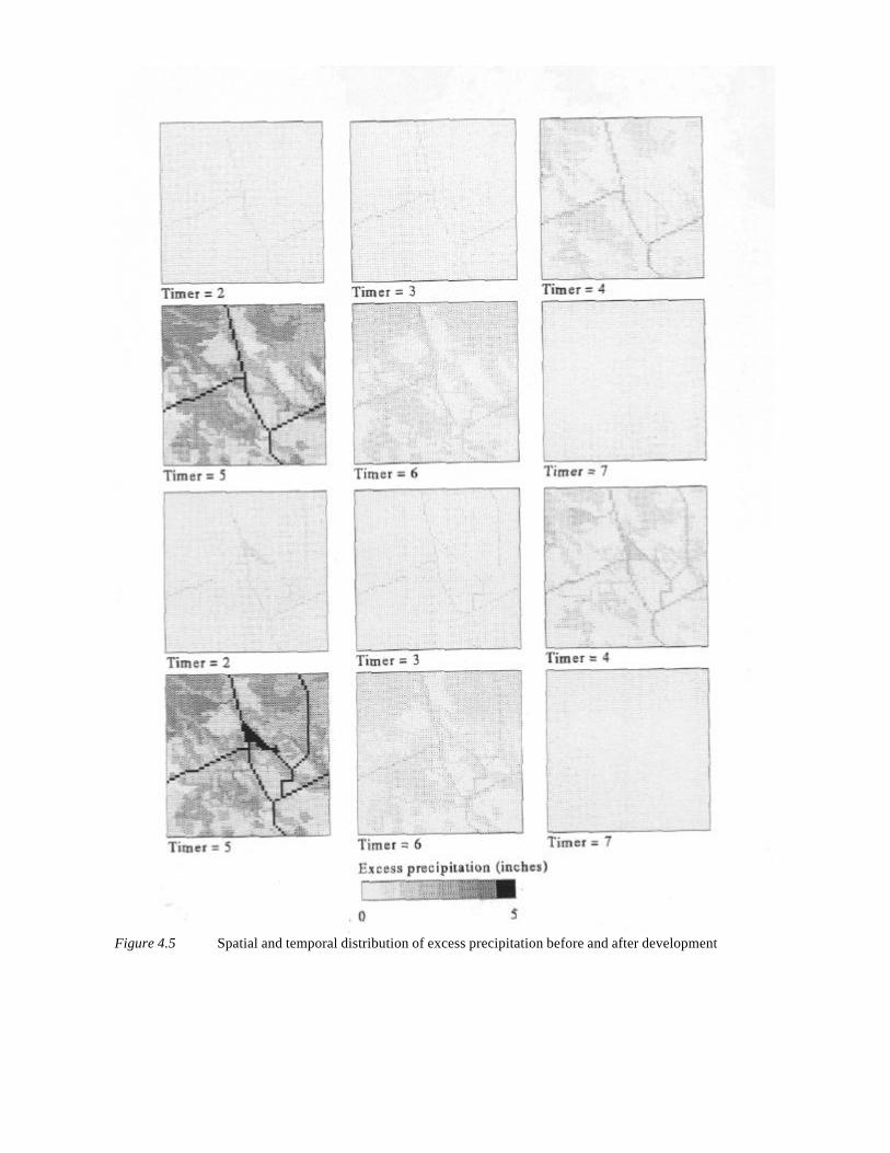
Figure 4.5 Spatial and temporal distribution of excess precipitation before and after development

4.4 DYNAMITE: A spatial modelling language for storage based modelling inPCRaster

In many problems of interest to physical geographers a mass budget of water, sediment, carbon or biomassprovides a useful framework within which the process model can be fitted. The mass budget (or energy budget)concept provides a well-founded physical basis which holds a model together. All mass and energy budgets (orbalances) rely on the physical principles of conservation of mass and energy and can be described using a simplestorage equation:

Inflow - Outflow = Net increase in storage (4.8)I - O = ∆S

Mass balance modelling implements a 'memory' in the system. The reaction of the system at time t is not only afunction of the inputs at time t, but also depends on the state (condition) of the model. The state of the model is aresult of all the behaviour in the past, and so the reaction of the system depends on the history of the system; thesystem contains a memory. As defined by Forrester [1968], a 'system' indicates a grouping of parts, componentsor objects that operate together with a common purpose, function or behaviour.

In the simplest type of storage models one storage is defined. For this single storage, the contents is determinedby (single or multiple) inflow and outflow. This type of models can be used to describe the outflow from areservoir or exponential or logistic growth of populations. More complex storage models have more than onestorage, and outflow from one storage may become inflow to another. It is clear that all storages show similar butnot identical behaviour. They all react to inflows and outflows, and their state is described with the simplestorage formula. The contents of the individual storages at a certain time t, however, may be different.

Transports describe the flows of energy and matter between storages. As such, they are a very importantcomponent related to the storages, since mass or energy can only be added to or subtracted from storages usingtransports. Transports are connected to storages, meaning they convey mass or energy from one storagecomponent to another. The behaviour of the transport elements, i.e. the amount of mass being conveyed using atransport is not implicitly defined, as is the case with the storage elements. The analysis of the system has toreveal this exact behaviour. The amount conveyed may be constant or a simple function of the state of thestorage it flows from, but it may also be a very complex function of the state of multiple storages in the systemand a reaction to multiple inputs. The relations describing these flows and transports may become very complex.The following general formulation may be given:

I - O = ∆S (4.9)I = f(S,...)O = f(S,...)

Solutions for this kind of problems can be analytical or numerical. Only the most simple cases of these problemsallow for analytical solutions, but usually numerical techniques have to be used to solve these problems.Numerical techniques require some discretisation of time. The time domain for which a solution has to be foundis divided into sufficiently small finite steps, for which the differential equations are solved. Simple techniques(Euler solutions of differential equations) use the value of St-1 to compute the values of It and Ot, but mayintroduce considerable errors. More advanced techniques (such as Runge-Kutta methods) try to solve theequations for It and Ot iteratively by making estimates for St, solve the equations for It and Ot based on thisestimate, and adjust the estimate of St accordingly. By repeatedly adjusting the estimations, these methods yielda more robust technique to solve the differential equations. The algorithms used to solve this type of problemsare well known from the mathematics for solving differential equations. For an extensive discussion of these isreferred to the handbooks on numerical techniques.

In his concepts on Systems Analysis Forrester [1968] introduces the auxiliary variables. These are additionalstatements and variables, which cannot be classified as storages or transports. These auxiliary variables are partof the transports equations, but subdivided and separated because they express concepts that have independentmeaning. Additionally, input variables can be defined. These components are also part of the transports, but theirvalues are not controlled by the state of the system. Inputs are determined by variables and processes outside thesystem.

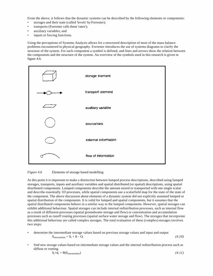
From the above, it follows that the dynamic systems can be described by the following elements or components:• storages and their state (called 'levels' by Forrester);• transports (Forrester calls them 'rates');• auxiliary variables; and• inputs or forcing functions.

Using the perceptions of Systems Analysis allows for a structured description of most of the mass balanceproblems encountered in physical geography. Forrester introduces the use of systems diagrams to clarify thestructure of the system. For each component a symbol is defined, and lines and arrows show the relation betweenthe components and the structure of the system. An overview of the symbols used in this research is given infigure 4.6.

Figure 4.6 Elements of storage based modelling

At this point it is important to make a distinction between lumped process descriptions, described using lumpedstorages, transports, inputs and auxiliary variables and spatial distributed (or spatial) descriptions, using spatialdistributed components. Lumped components describe the amount stored or transported with one single scalarand describe essentially 1D processes, while spatial components use a scalarfield map for the state of the state ofthe component. The above discussion about elements of a dynamic system did not explicitly assumed lumped orspatial distribution of the components. It is valid for lumped and spatial components, but it assumes that thespatial distributed components behave in a similar way to the lumped components. However, spatial storages canexhibit additional behaviour. Spatial storages can include internal redistribution processes, such as internal flowas a result of diffusion processes (spatial groundwater storage and flow) or concentration and accumulationprocesses such as runoff routing processes (spatial surface water storage and flow). The storages that incorporatethis additional behaviour are called complex storages. The total evaluation of these (complex) storages involvestwo steps:

• determine the intermediate storage values based on previous storage values and input and outputSintermediate = St + It - Ot (4.10)

• find new storage values based on intermediate storage values and the internal redistribution process such asdiffuse or routing.

St+dt = R(Sintermediate) (4.11)

withR = one of the internal redistribution processes.

DYNAMITE is a script language based on the concepts of system components. It extends the concepts of theDYNAMO interpreter [Forrester, 1968] and the STELLA II modelling program [eg. McDonnell and MacMillan,1993] into spatial dynamic modelling. The advantages over the plain use of PCRaster for dynamic modelling isthat is allows for a better structuring. DYNAMITE allows for the definition of the components of the system,and for each component describing the behaviour that is specific for that component. Standard behaviour ofstorages is that they are updated each timestep with the inputs and outputs. This is the regular behaviour of eachentity defined as a storage, so there is no need to specify this behaviour explicitly. The initial values for storageshould be assigned to each entity of the storage type individually, so the definition of a storage includes theassignment of an initial value. In addition to the sections as described in section 4.2, DYNAMITE recognises thekeywords storage, identifying a storage definition, and transport, identifying the definition of a transportcomponent. Auxiliary variables are not linked to a special keyword, since they are part of the dynamic sectionalready defined.

The storage keyword identifies the definition of one storage component. The initial value of the storage is setwith the assignment of the initial statement. The syntax of one storage component is:

storage Identifier: initial Identifier = initialExpression;

The definition of storages may contain optional routing sections, implementing one of the routing andredistribution functions as defined in section 4.5. The routing definition is preceded by the keyword routing.Storage definitions may include optional report statements. Examples of storage definitions are:

storage SoilWater: initial SoilWater = 0;

and

storage SurfaceWater: initial SurfaceWater = 0; routing accu(Ldd, SurfaceWater); report Discharge = flux(SurfaceWater);

The transport keyword identifies the definition of one transport component. The identification of a transport isthrough the definition of an identifier defining the transport name and the description of the storage it flowsfrom and of the storage it flows to. If the definition of one of the connected storages is omitted, it is assumed thetransport is from an infinite source or to an infinite sink. Transport definitions may include optional reportstatements. The syntax of the transport definition is

transport Identifier StoragesConnectedStoragesConnected from id to id

from idto id

Examples of the use of transports are:transport Precipitation to SoilWater: Precipitation = timeinputscalar(PrecipitationInput,PrecipitationId);

transport RS from SoilWater to SurfaceWater: RS = 0.2 * SoilWater;

transport AE from SoilWater: AE = ... * timeinputscalar(TemperatureInput,TemperatureID) + .....;

Examples of the use of DYNAMITE for dynamic modelling are given in chapter 5 and 6.

4.5 Geomorphologic landscape and catchment analysis tools

4.5.1 Introduction

The example of excess precipitation of section 4.3 is one dimensional, i.e. the model assumes that each cell inthe area is independent and unique. In reality, this is not so: excess rainfall in one cell can flow to adjacent cells,causing flooding even if these adjacent cells themselves do not suffer their own excess. The lateral movement ofwater is part of a more general problem of the spatio temporal movement of material, which is described in thisand the next section.

Digital Elevation Models (DEM) are defined as GIS data sets that contain information on the topographicelevation of the area. Although they do not necessarily have to be implemented in raster structures, in thefollowing discussion it is assumed the DEM is implemented in such a structure. The elevation is usually linkedto the centre point of each cell. The recorded value might represent an exact, measured value, an interpolatedvalue for that point, or an average over the whole cell. DEM's can be used to derive a large amount ofinformation about the morphology of the landscape using the neighbourhood operations to calculate slope andaspect [Burrough, 1986]. Catchment areas and overland flow paths are closely related to slope, aspect andinflection information, but they also represent a number of specific problems that cannot be described using thestandard neighbourhood operators. This special nature of this type of problems has led to the development of aset of geomorphologic and landscape analysis tools especially designed for processing raster DEM's [Marks etal., 1984; Band, 1986; Morris and Heerdegen, 1988; Jenson and Domingue, 1988; Moore et al., 1993; Maidment,1993a].

The current generation of geomorphologic landscape and catchment analysis tools for raster grids are all basedon the concepts of the local drain direction (LDD). This concept analyses each cell in the DEM, and determinesthe slope in each of the eight directions connecting the cell to its neighbours. For each grid cell the steepestdownward direction defines the direction in which (potential) surface water from that cell would flow. Thisdirection is called the local drain direction. The actual availability of surface water is not essential, the localdrain direction is defined purely based on the slopes and slope directions in the Digital Elevation Model. Theanalysis is performed by placing a 3 x 3 window over the raster map, and by analysing this 3 x 3 window, thelocal drain direction for the centre cell can be found. If the local drain direction of the current cell is found, the 3x 3 window is moved to the next cell.

It is worth realising that the DEM represents a potential surface. In most cases we are analysing the land surfacewhich represents 'potential gravitational energy', but the concept and methods could be applied to any other kindof potential: concentrations, electric charge, money, etcetera. The DEM is a nice, easily visualisable example.

If for each cell in the grid a local drain direction is defined, a flow net can be constructed by connecting the localdrain direction of the current cell to the local drain direction of downward cell (which is the cell the current cellwill drain into). Following this flow net (which is a directed acyclic graph) downstream from a certain locationin a catchment leads to the outlet point of the catchment. From this outlet point, we can determine all the gridcells eventually draining through this point and mark them as part of the catchment, or we can use the local draindirection network as the network through which water and material will be transported.

The DEM only provides an approximation of the true elevation of an area. A DEM is a discretisation of reality,meaning that below some level, detail is lost, and only approximated at a coarser level. Because of mismatch inresolution, the DEM may fail to indicate how drainage links together. Narrow valleys and channels can bemissed, and spurious 'pits' can occur when the grid picks up an isolated part of a valley or channel. As some reallandscapes have real closed depressions (ponds, lakes) it is essential to be able to distinguish between artifactsand real phenomena.

The routines implementing these actions were developed by Marks et al. [1984], Band [1986], Morris andHeerdegen [1988] and Jenson and Domingue [1988]. In rugged areas with distinct slopes this approach is verystraightforward, but the nemesis of this approach is in the handling of flat areas, depressions and pits. Theprocedures to create the local drain direction map as presented here are based on the algorithms presented inliterature. However, the algorithms for finding local drain direction in flat areas and pits have been modifiedconsiderably. Also, the tools to analyse the landscape and the catchments and the tools for transport along the

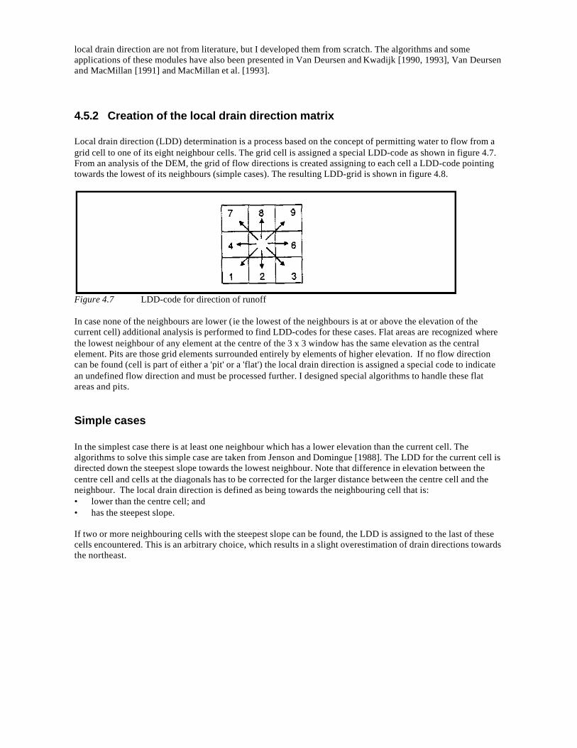
local drain direction are not from literature, but I developed them from scratch. The algorithms and someapplications of these modules have also been presented in Van Deursen and Kwadijk [1990, 1993], Van Deursenand MacMillan [1991] and MacMillan et al. [1993].

4.5.2 Creation of the local drain direction matrix

Local drain direction (LDD) determination is a process based on the concept of permitting water to flow from agrid cell to one of its eight neighbour cells. The grid cell is assigned a special LDD-code as shown in figure 4.7.From an analysis of the DEM, the grid of flow directions is created assigning to each cell a LDD-code pointingtowards the lowest of its neighbours (simple cases). The resulting LDD-grid is shown in figure 4.8.

Figure 4.7 LDD-code for direction of runoff

In case none of the neighbours are lower (ie the lowest of the neighbours is at or above the elevation of thecurrent cell) additional analysis is performed to find LDD-codes for these cases. Flat areas are recognized wherethe lowest neighbour of any element at the centre of the 3 x 3 window has the same elevation as the centralelement. Pits are those grid elements surrounded entirely by elements of higher elevation. If no flow directioncan be found (cell is part of either a 'pit' or a 'flat') the local drain direction is assigned a special code to indicatean undefined flow direction and must be processed further. I designed special algorithms to handle these flatareas and pits.

Simple cases

In the simplest case there is at least one neighbour which has a lower elevation than the current cell. Thealgorithms to solve this simple case are taken from Jenson and Domingue [1988]. The LDD for the current cell isdirected down the steepest slope towards the lowest neighbour. Note that difference in elevation between thecentre cell and cells at the diagonals has to be corrected for the larger distance between the centre cell and theneighbour. The local drain direction is defined as being towards the neighbouring cell that is:• lower than the centre cell; and• has the steepest slope.

If two or more neighbouring cells with the steepest slope can be found, the LDD is assigned to the last of thesecells encountered. This is an arbitrary choice, which results in a slight overestimation of drain directions towardsthe northeast.

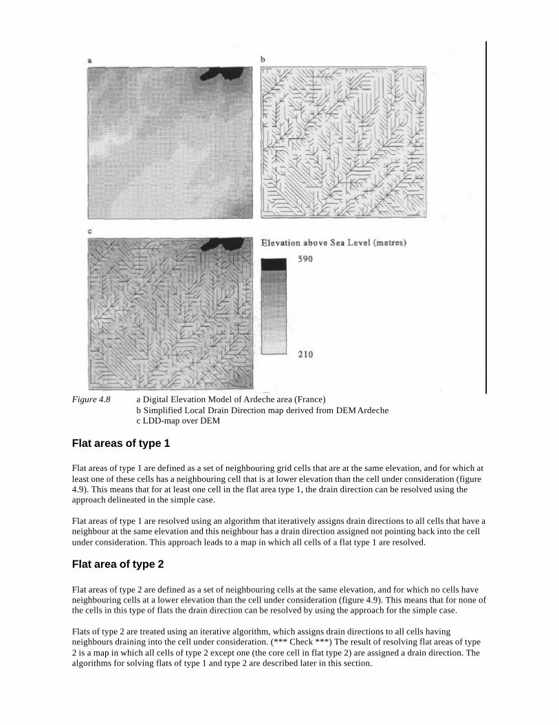
Figure 4.8 a Digital Elevation Model of Ardeche area (France)b Simplified Local Drain Direction map derived from DEM Ardechec LDD-map over DEM

Flat areas of type 1

Flat areas of type 1 are defined as a set of neighbouring grid cells that are at the same elevation, and for which atleast one of these cells has a neighbouring cell that is at lower elevation than the cell under consideration (figure4.9). This means that for at least one cell in the flat area type 1, the drain direction can be resolved using theapproach delineated in the simple case.

Flat areas of type 1 are resolved using an algorithm that iteratively assigns drain directions to all cells that have aneighbour at the same elevation and this neighbour has a drain direction assigned not pointing back into the cellunder consideration. This approach leads to a map in which all cells of a flat type 1 are resolved.

Flat area of type 2

Flat areas of type 2 are defined as a set of neighbouring cells at the same elevation, and for which no cells haveneighbouring cells at a lower elevation than the cell under consideration (figure 4.9). This means that for none ofthe cells in this type of flats the drain direction can be resolved by using the approach for the simple case.

Flats of type 2 are treated using an iterative algorithm, which assigns drain directions to all cells havingneighbours draining into the cell under consideration. (*** Check ***) The result of resolving flat areas of type2 is a map in which all cells of type 2 except one (the core cell in flat type 2) are assigned a drain direction. Thealgorithms for solving flats of type 1 and type 2 are described later in this section.

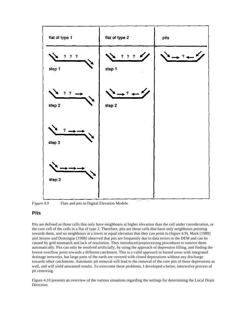
Figure 4.9 Flats and pits in Digital Elevation Models

Pits

Pits are defined as those cells that only have neighbours at higher elevation than the cell under consideration, orthe core cell of the cells in a flat of type 2. Therefore, pits are those cells that have only neighbours pointingtowards them, and no neighbours at a lower or equal elevation that they can point to (figure 4.9). Mark [1988]and Jenson and Domingue [1988] observed that pits are frequently due to data errors in the DEM and can becaused by grid mismatch and lack of resolution. They introduced preprocessing procedures to remove themautomatically. Pits can only be resolved artificially, by using the approach of depression filling, and finding thelowest overflow point towards a different catchment. This is a valid approach in humid areas with integrateddrainage networks, but large parts of the earth are covered with closed depressions without any dischargetowards other catchments. Automatic pit removal will lead to the removal of the core pits of these depressions aswell, and will yield unwanted results. To overcome these problems, I developed a better, interactive process ofpit removing.

Figure 4.10 presents an overview of the various situations regarding the settings for determining the Local DrainDirection.

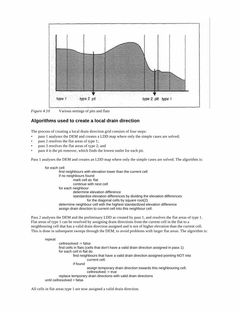
Figure 4.10 Various settings of pits and flats

Algorithms used to create a local drain direction

The process of creating a local drain direction grid consists of four steps:• pass 1 analyses the DEM and creates a LDD map where only the simple cases are solved;• pass 2 resolves the flat areas of type 1;• pass 3 resolves the flat areas of type 2; and• pass 4 is the pit remover, which finds the lowest outlet for each pit.

Pass 1 analyses the DEM and creates an LDD map where only the simple cases are solved. The algorithm is:

for each cellfind neighbours with elevation lower than the current cellif no neighbours found

mark cell as flatcontinue with next cell

for each neighbourdetermine elevation differencestandardize elevation differences by dividing the elevation differences

for the diagonal cells by square root(2)determine neighbour cell with the highest standardized elevation differenceassign drain direction to current cell into this neighbour cell.

Pass 2 analyses the DEM and the preliminary LDD as created by pass 1, and resolves the flat areas of type 1.Flat areas of type 1 can be resolved by assigning drain directions from the current cell in the flat to aneighbouring cell that has a valid drain direction assigned and is not of higher elevation than the current cell.This is done in subsequent sweeps through the DEM, to avoid problems with larger flat areas. The algorithm is:

repeatcellresolved := falsefind cells in flats (cells that don't have a valid drain direction assigned in pass 1)for each cell in flat do

find neighbours that have a valid drain direction assigned pointing NOT intocurrent cell.

if foundassign temporary drain direction towards this neighbouring cell.cellresolved := true

replace temporary drain directions with valid drain directionsuntil cellresolved = false

All cells in flat areas type 1 are now assigned a valid drain direction.

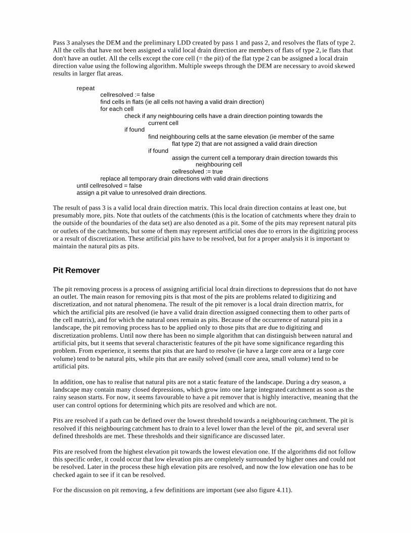
Pass 3 analyses the DEM and the preliminary LDD created by pass 1 and pass 2, and resolves the flats of type 2.All the cells that have not been assigned a valid local drain direction are members of flats of type 2, ie flats thatdon't have an outlet. All the cells except the core cell (= the pit) of the flat type 2 can be assigned a local draindirection value using the following algorithm. Multiple sweeps through the DEM are necessary to avoid skewedresults in larger flat areas.

repeatcellresolved := falsefind cells in flats (ie all cells not having a valid drain direction)for each cell

check if any neighbouring cells have a drain direction pointing towards thecurrent cell

if foundfind neighbouring cells at the same elevation (ie member of the same

flat type 2) that are not assigned a valid drain directionif found

assign the current cell a temporary drain direction towards thisneighbouring cell

cellresolved := truereplace all temporary drain directions with valid drain directions

until cellresolved = falseassign a pit value to unresolved drain directions.

The result of pass 3 is a valid local drain direction matrix. This local drain direction contains at least one, butpresumably more, pits. Note that outlets of the catchments (this is the location of catchments where they drain tothe outside of the boundaries of the data set) are also denoted as a pit. Some of the pits may represent natural pitsor outlets of the catchments, but some of them may represent artificial ones due to errors in the digitizing processor a result of discretization. These artificial pits have to be resolved, but for a proper analysis it is important tomaintain the natural pits as pits.

Pit Remover

The pit removing process is a process of assigning artificial local drain directions to depressions that do not havean outlet. The main reason for removing pits is that most of the pits are problems related to digitizing anddiscretization, and not natural phenomena. The result of the pit remover is a local drain direction matrix, forwhich the artificial pits are resolved (ie have a valid drain direction assigned connecting them to other parts ofthe cell matrix), and for which the natural ones remain as pits. Because of the occurrence of natural pits in alandscape, the pit removing process has to be applied only to those pits that are due to digitizing anddiscretization problems. Until now there has been no simple algorithm that can distinguish between natural andartificial pits, but it seems that several characteristic features of the pit have some significance regarding thisproblem. From experience, it seems that pits that are hard to resolve (ie have a large core area or a large corevolume) tend to be natural pits, while pits that are easily solved (small core area, small volume) tend to beartificial pits.

In addition, one has to realise that natural pits are not a static feature of the landscape. During a dry season, alandscape may contain many closed depressions, which grow into one large integrated catchment as soon as therainy season starts. For now, it seems favourable to have a pit remover that is highly interactive, meaning that theuser can control options for determining which pits are resolved and which are not.

Pits are resolved if a path can be defined over the lowest threshold towards a neighbouring catchment. The pit isresolved if this neighbouring catchment has to drain to a level lower than the level of the pit, and several userdefined thresholds are met. These thresholds and their significance are discussed later.

Pits are resolved from the highest elevation pit towards the lowest elevation one. If the algorithms did not followthis specific order, it could occur that low elevation pits are completely surrounded by higher ones and could notbe resolved. Later in the process these high elevation pits are resolved, and now the low elevation one has to bechecked again to see if it can be resolved.

For the discussion on pit removing, a few definitions are important (see also figure 4.11).

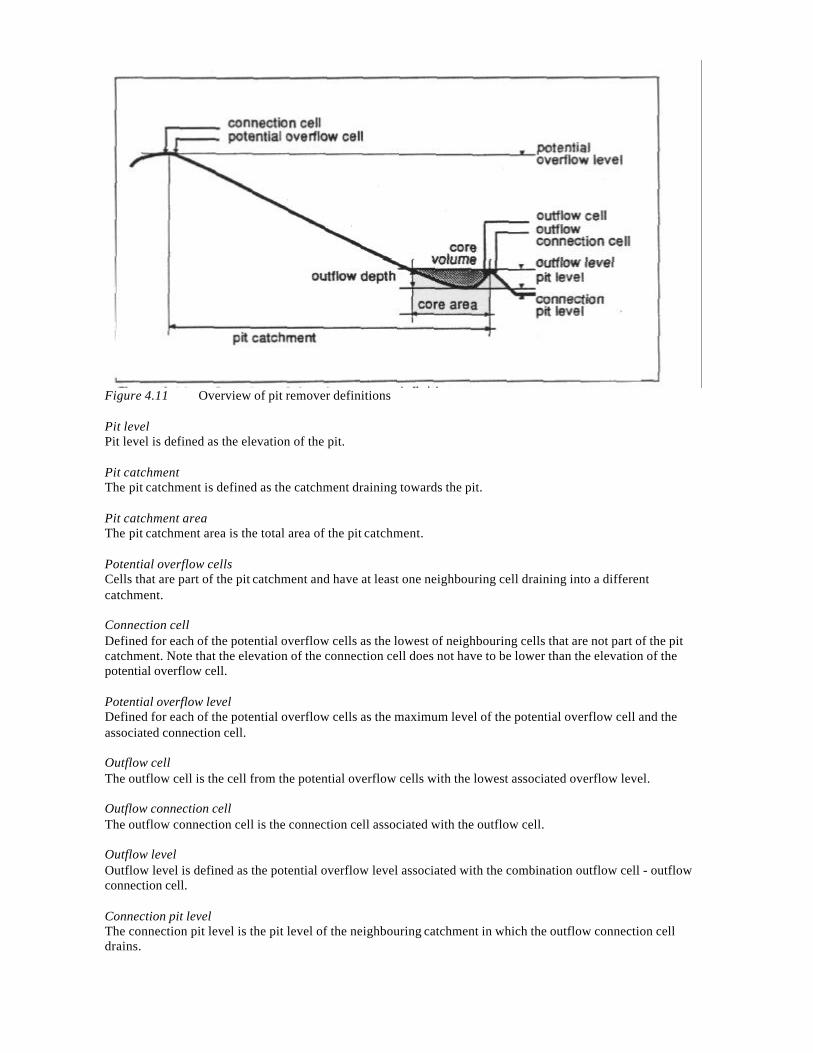
Figure 4.11 Overview of pit remover definitions

Pit levelPit level is defined as the elevation of the pit.

Pit catchmentThe pit catchment is defined as the catchment draining towards the pit.

Pit catchment areaThe pit catchment area is the total area of the pit catchment.

Potential overflow cellsCells that are part of the pit catchment and have at least one neighbouring cell draining into a differentcatchment.

Connection cellDefined for each of the potential overflow cells as the lowest of neighbouring cells that are not part of the pitcatchment. Note that the elevation of the connection cell does not have to be lower than the elevation of thepotential overflow cell.

Potential overflow levelDefined for each of the potential overflow cells as the maximum level of the potential overflow cell and theassociated connection cell.

Outflow cellThe outflow cell is the cell from the potential overflow cells with the lowest associated overflow level.

Outflow connection cellThe outflow connection cell is the connection cell associated with the outflow cell.

Outflow levelOutflow level is defined as the potential overflow level associated with the combination outflow cell - outflowconnection cell.

Connection pit levelThe connection pit level is the pit level of the neighbouring catchment in which the outflow connection celldrains.

Outflow depthThe outflow depth is defined as the difference between outflow level and pit level

Core areaThe core area of a pit is the area that contains all the cells in the pit catchment with an elevation lower than theoutflow level.

Core volumeThe core volume of the pit is the total volume in the pit catchment between the hypsometric surface asrepresented by the DEM and the outflow level.

Pit input water layerPit input water layer is defined as the layer of water (in most cases representing effective precipitation) in the pitcatchment necessary to fill the core volume completely. By definition, the pit input water layer equals corevolume divided by pit catchment area.

Core Area thresholdThe core area threshold is a threshold on the area of the cells that are below the level of overflow. This is thetotal area of the core of the depression. The area threshold is used so that if the core area of the depression islarger than the area threshold, the pit will not be resolved.

Overflow Depth thresholdThe overflow depth is defined as the difference between the overflow level and the elevation of the pit cell. Ifthis overflow depth is larger than the overflow depth threshold, the pit will not be resolved.

Core Volume thresholdThe core volume is defined as the total volume that is needed to fill the core area to the overflow level. Thevolume threshold sets the upper limit of the volume, if the core volume is larger than the volume threshold, thepit will not be resolved.

Pit input water level thresholdThe pit input water level is defined as the core volume of the pit divided by the area of the catchment drainingtowards the pit. The pit input water level threshold is set to solve only those pits that need a pit input water levelless than the pit input water level threshold.

Reversing drain directionsOnce the outflow cell has been found, the original path from this outflow cell towards the pit has to be reversed,that is, a connection is made between the pit and the outflow cell. The outflow cell is assigned a LDD-codetowards the connection cell. Now, by tracing the LDD from a certain cell within the pit catchment, the LDD willfirst travel through the pit, then towards the outflow cell, from the outflow cell into the connection cell and fromthe connection cell towards the pit of the neighbouring catchment. Once this process is finished, the current pithas actually been removed, the local drain direction matrix is no longer discontinuous in the core of the pit.

Pit remover optionsThe pit remover can be regarded as representing two different physical processes. The first process is where thedepression is filled by water and sediment, until the depression bottom (pit level) is at the same level as theoutflow level. The pit then is no longer a pit, but becomes part of a flat area type 1. This process can bedescribed by the pit remover using the option depression filling. In this case, the pit remover assigns newelevation values to the cells in the DEM that are part of the core area. All the core cells are assigned an elevationvalue equal to the outflow level, so the pit is effectively removed from the DEM. The second process is that ofchannel cutting. If enough water is available, the river may cut a channel through the barrier separating the pitarea from the potential overflow area. This process can be described with the channel cut option of thepitremover. This option assigns new values on the connection path between the pit of the catchment towards thecore of the potential overflow area. The new values on this path are equal to the pit level, thus removing the pitand creating a flat area type 1.

The algorithm for pit removing is

for current pit = highest to lowest dofind pit catchment for current pitfind potential overflow cells

if no potential overflow cells are foundcurrent pit cannot be resolvedcontinue with next pit

for each potential overflow cell dofind potential overflow level

find outflow cell and outflow connection cellfind connection pit levelif connection pit level larger than current pit level

current pit cannot be resolvedcontinue with next pit

find overflow depthif overflow depth larger than level threshold

current pit cannot be resolvedcontinue with next pit

find core areaif core area larger than area threshold

current pit cannot be resolvedcontinue with next pit

find core volumeif core volume larger than volume threshold

current pit cannot be resolvedcontinue with next pit

find pit input water layerif pit input water layer larger than pit input water level threshold

current pit cannot be resolvedcontinue with next pit

unblock current pit by reversing the drain directions on the path from the overflow cellto the pit cell and assigning a drain direction towards the connection cell forthe overflow cell.

if necessaryadjust elevation of DEM by filling the depression

if necessaryadjust elevation of DEM by cutting a channel.

continue with next pit

The pit remover results in a DEM that has pits which are considered natural features of the landscape, and noartifacts due to digitizing, interpolation and discretization. At least one pit will be present, which is consideredthe outlet point of the catchment.

The process of creating a LDD-map from a DEM is implemented in the function makeldd. The syntax for thisfunction is

<LddMap>= makeldd(<DEM>, <Overflow Depth Threshold>, <Core Volume Threshold>,<Core Area Threshold>, <Pit input water layer Threshold>).

The associated function that returns the modified DEM is

<DEM>= demmakeldd(<DEM>, <Overflow Depth Threshold>,<Core Volume Threshold>, <Core Area Threshold>,<Pit input water layer Threshold>)

These two functions can be called separately, if one only needs the LddMap or the modified DEM, but in caseboth results are needed, the two functions can be combined. The syntax then becomes:

<LddMap>,<DEM>= makeldd,demmakeldd(<DEM>, <Overflow Depth Threshold>,<Core Volume Threshold>, <Core Area Threshold>,<Pit input water layer Threshold>)

This mechanism works for combining all complementary functions, which have the same parameter list.

4.5.3 Catchment analysis

As the LDD-grid indicates the potential flow path, it is the starting point for a number of geomorphologicanalyses and can be used for as a basis for network analysis and flow routing. For simple catchment analysis,several techniques will be described. They include the determination of catchments above pits and outlets, thedetermination of upstream areas for the cells in a catchment and stream network ordering. The algorithms forcatchment delineation and determination of upstream elements are taken from literature [Morris and Heerdegen,1988]. I developed more complex functions that describe the result of dynamically transporting material throughthe LDD-map. All these functions are introduced in this section.

Finding pits

The first function defined is for finding all the pits in a LDD-map. The algorithm for this function scans theLDD-map and returns a boolean map with 'true' for the cells that are pits, and 'false' elsewhere.

The syntax of the function is:

<ResultMap> = pit(<LddMap>)

Determination of the downstream value

The function downstream returns the value of the downstream cell in the current cell. For pit cells, this functionreturns the value of the pit cell. This function may seem a bit superfluous, but is useful in combination with therouting functions. The syntax of the function is:

<ResultMap>=downstream(<LddMap>)

Determination of catchments for specified points

Each pit and outlet may be considered a location for which the watershed can be determined. The LDD assignedto each grid element can be used to find all the elements ultimately draining through the same cell, thusbelonging to the catchment area of this cell. A recursive algorithm (described in detail by Morris and Heerdegen[1988]) follows the assigned drain directions upslope from the specified points, labels all the elements it travelsthrough, until no further cells point into the last element checked (ie the catchment boundary is reached). It thenfalls back until it finds another unique flow path, follows this path upslope, until all flow paths in the catchmentare checked. This results in a map with all the elements belonging to a catchment labelled with a uniqueidentifier as part of the catchment.

The algorithm used is (from Morris and Heerdegen [1988]):

procedure is_upstream(row,col)go_upstream(9,row+1,col-1)go_upstream(8,row+1,col)go_upstream(7,row+1,col+1)go_upstream(6,row,col-1)go_upstream(4,row,col+1)go_upstream(3,row-1,col-1)go_upstream(2,row-1,col)go_upstream(1,row-1,col+1)setcatchment(row,col,catchmentID)

procedure go_upstream(testlddcode,row,col)if getlddcode(row,col) = testlddcode then

is_upstream(row,col)

for each specified cell docatchmentID = getcatchmentIDis_upstream(row,col)

The syntax of the function is:

<ResultMap> = catchment(<LddMap>,<PointsMap>)

To find catchments for all of the pits in the DEM, the following function is appropriate:

<ResultMap> = catchment(<LddMap>,cellId(pits(<LddMap>)))

Distances measured through the LDD-map

With slight modifications the algorithm can determine the length of the path from each cell in the catchments tothe outlet of the catchments. For this analysis a 'resistance-value 'is incremented for each element travelledthrough on the way upslope. For each cell this will give the so called 'resistance to outlet' or 'path length tooutlet'.

This algorithm is implemented in the function ldddist. It determines 'weighted resistances 'to the outlet, this is,for each cell it travels through in the upslope direction it adds the value given in a 'resistance-overlay' to theresistance already travelled through. If no 'resistance-overlay' is specified, for each cell travelled through thecell-size is added to the resistance-counter, resulting in a map containing 'distance to outlet' or 'dispersion area'.

The pseudo code for the algorithms for this operation is:

procedure ldd_res_is_upstream(row,col, total_res, prev_cell_res)cell_res:=getcellresistance(row,col)total_res :=total_res+0.5*cell_res+0.5*prev_cell_resistanceset_total_resistance(row,col,total_res)ldd_res_go_upstream(9,row+1,col-1,total_res,cell_res)ldd_res_go_upstream(8,row+1,col,total_res,cell_res)ldd_res_go_upstream(7,row+1,col+1,total_res,cell_res)ldd_res_go_upstream(6,row,col-1,total_res,cell_res)ldd_res_go_upstream(4,row,col+1,total_res,cell_res)ldd_res_go_upstream(3,row-1,col-1,total_res,cell_res)ldd_res_go_upstream(2,row-1,col,total_res,cell_res)ldd_res_go_upstream(1,row-1,col+1,total_res,cell_res)

procedure ldd_res_go_upstream(testlddcode,row,col,total_res,prev_cell_res)if getlddcode(row,col) = testlddcode then

ldd_res_is_upstream(row,col,total_res,prev_cell_res)

for each specified cell docell_res:=getcellresistance(row,col)ldd_res_is_upstream(row,col,0,cell_res)

The syntax of the function is:

< ResultMap > = ldddist(<LddMap>,<ResistanceMap>)

to find the resistance from each point to the outlet through the resistance map.

To find the distance of each cell to the outlet, the function call is:

< ResultMap> = ldddist(<LddMap>,1);or

< ResultMap> = ldddist(<LddMap>,cellsize(LddMap));

Network ordering algorithms

A modified version of the above algorithm can be used to find stream orders in the river network. Theclassification of stream networks was originally developed by Horton [1945], and modified by Strahler [1964].In the scheme developed by Strahler, the smallest channels are designated order 1. Where two channels of order

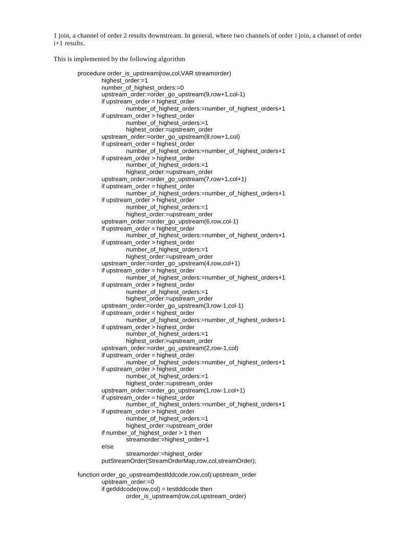
1 join, a channel of order 2 results downstream. In general, where two channels of order i join, a channel of orderi+1 results.

This is implemented by the following algorithm

procedure order_is_upstream(row,col,VAR streamorder)highest_order:=1number_of_highest_orders:=0upstream_order:=order_go_upstream(9,row+1,col-1)if upstream_order = highest_order

number_of_highest_orders:=number_of_highest_orders+1if upstream_order > highest_order

number_of_highest_orders:=1highest_order:=upstream_order

upstream_order:=order_go_upstream(8,row+1,col)if upstream_order = highest_order

number_of_highest_orders:=number_of_highest_orders+1if upstream_order > highest_order

number_of_highest_orders:=1highest_order:=upstream_order

upstream_order:=order_go_upstream(7,row+1,col+1)if upstream_order = highest_order

number_of_highest_orders:=number_of_highest_orders+1if upstream_order > highest_order

number_of_highest_orders:=1highest_order:=upstream_order

upstream_order:=order_go_upstream(6,row,col-1)if upstream_order = highest_order

number_of_highest_orders:=number_of_highest_orders+1if upstream_order > highest_order

number_of_highest_orders:=1highest_order:=upstream_order

upstream_order:=order_go_upstream(4,row,col+1)if upstream_order = highest_order

number_of_highest_orders:=number_of_highest_orders+1if upstream_order > highest_order

number_of_highest_orders:=1highest_order:=upstream_order

upstream_order:=order_go_upstream(3,row-1,col-1)if upstream_order = highest_order

number_of_highest_orders:=number_of_highest_orders+1if upstream_order > highest_order

number_of_highest_orders:=1highest_order:=upstream_order

upstream_order:=order_go_upstream(2,row-1,col)if upstream_order = highest_order

number_of_highest_orders:=number_of_highest_orders+1if upstream_order > highest_order

number_of_highest_orders:=1highest_order:=upstream_order

upstream_order:=order_go_upstream(1,row-1,col+1)if upstream_order = highest_order

number_of_highest_orders:=number_of_highest_orders+1if upstream_order > highest_order

number_of_highest_orders:=1highest_order:=upstream_order

if number_of_highest_order > 1 thenstreamorder:=highest_order+1

elsestreamorder:=highest_order

putStreamOrder(StreamOrderMap,row,col,streamOrder);

function order_go_upstream(testlddcode,row,col):upstream_orderupstream_order:=0if getlddcode(row,col) = testlddcode then

order_is_upstream(row,col,upstream_order)

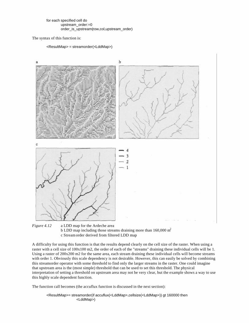
for each specified cell doupstream_order:=0order_is_upstream(row,col,upstream_order)

The syntax of this function is:

<ResultMap> = streamorder(<LddMap>)

Figure 4.12 a LDD map for the Ardeche areab LDD map including those streams draining more than 160,000 m2

c Stream order derived from filtered LDD map

A difficulty for using this function is that the results depend clearly on the cell size of the raster. When using araster with a cell size of 100x100 m2, the order of each of the "streams" draining these individual cells will be 1.Using a raster of 200x200 m2 for the same area, each stream draining these individual cells will become streamswith order 1. Obviously this scale dependency is not desirable. However, this can easily be solved by combiningthis streamorder operator with some threshold to find only the larger streams in the raster. One could imaginethat upstream area is the (most simple) threshold that can be used to set this threshold. The physicalinterpretation of setting a threshold on upstream area may not be very clear, but the example shows a way to usethis highly scale dependent function.

The function call becomes (the accuflux function is discussed in the next section):

<ResultMap>= streamorder(if accuflux(<LddMap>,cellsize(<LddMap>)) gt 160000 then <LddMap>)

Using this function, the LDD network (figure 4.12a) is first filtered to include only those streams that drainmore than 160000 m2 (figure 4.12b), and for this network the stream order is determined (figure 4.12c).

4.5.4 Accumulation of material through the LDD-map

The algorithm used to find upstream area requires a slight modification of the algorithms used to find thecatchments. Each time the algorithm falls back in the direction of the pit or outlet it increments a counter foreach element it passes through. The result is a map with each element being labelled with the number of cellsdraining through it.

The syntax of the function is:

<ResultMap> = accuflux(<LddMap>,<AmountMap>)

To get a map with number of upstream cells for each cell in the LddMap, the following command is suitable:

<ResultMap> = accuflux(<LddMap>,1)

The map with upstream area can be derived using:

<ResultMap> = accuflux(<LddMap>,cellsize(LddMap))

The pseudo code for this operation is:

procedure accu_is_upstream(row,col, VAR accuAmount)accu_go_upstream(9,row+1,col-1,upstreamAmount)accuAmount:=accuAmount + upstreamAmountaccu_go_upstream(8,row+1,col,upstreamamount)accuAmount:=accuAmount + upstreamAmountaccu_go_upstream(7,row+1,col+1,upstreamamount)accuAmount:=accuAmount + upstreamAmountaccu_go_upstream(6,row,col-1,upstreamamount)accuAmount:=accuAmount + upstreamAmountaccu_go_upstream(4,row,col+1,upstreamamount)accuAmount:=accuAmount + upstreamAmountaccu_go_upstream(3,row-1,col-1,upstreamamount)accuAmount:=accuAmount + upstreamAmountaccu_go_upstream(2,row-1,col,upstreamamount)accuAmount:=accuAmount + upstreamAmountaccu_go_upstream(1,row-1,col+1,upstreamamount)accuAmount:=accuAmount + upstreamAmountsetaccuAmount(row,col,accuAmount)

procedure accu_go_upstream(testlddcode,row,col,VAR accuAmount)accuAmount:=0if getlddcode(row,col) = testlddcode then

accu_is_upstream(row,col,accuAmount)

for each specified cell doaccuAmount:=0accu_is_upstream(row,col,accuAmount)

Complex accumulation operators

The above described accuflux function can be used to evaluate the amount of water that flows through eachpoint through the drainage network. However, it is only a very simple approach to this type of transport.Although the approach can be used to be linked to a water balance determining the amount of water that isavailable for transport through the drainage network, it cannot accommodate for transport phenomena wherelosses occur during the transport process, or which are subject to threshold values that have to be exceededbefore transport occurs. I developed eight functions that describe these processes more accurately.

Accumulation through the LDD and losses may occur as a result of four different mechanisms.• Transport capacity of the channel is limited. This is the case for water flowing through pipes and along

hydraulic structures, or sediment transport that is limited by the water velocity.• Transport will only occur if a certain threshold of losses has been reached. This is the case for overland flow

that will only develop once a certain loss has occurred, saturating the soil. This mechanism can also be usedto describe phenomena such as losses from the streamflow due to infiltration of river water through theriverbed.

• Withdrawal of a fraction of material from the stream. This enables the description of phenomena such as aloss of a certain ratio of organic matter over a river stretch.

• Transport occurs once a certain trigger value has been exceeded. This may be the case with landslides,where the soil has to be saturated first before all water (and soil) will be transported downhill, or avalancheswhere the total amount of snow will come down once triggered.

Each of these mechanisms yield two result maps, one map containing the amount of material transported (theflux through the system), and one map containing the amount of matter lost or left behind in each cell (the stateof the system). Accordingly, each mechanism is described using two functions: one yields the flux through thesystem (the ....Flux-functions), while the second one yields the state of the system (the ...State-function).

The mechanisms are implemented in the following functions:• For the limited transport capacity (LTC) case:

<LossesMap>=AccuLTCState(<LddMap>,<AmountMap>,<TransportCapacityMap>)and

<FluxMap>=AccuLTCFlux(<LddMap>,<AmountMap>,<TransportCapacityMap>).

• For the threshold transport (TT) case:

<LossesMap>=AccuTTState(<LddMap>,<AmountMap>,<TransportThresholdMap>)and

<FluxMap>=AccuTTFlux(<LddMap>,<AmountMap>,<TransportThresholdMap>)

• For the fraction withdrawal (Fraction) case:

<LossesMap>=AccuFractionState(<LddMap>,<AmountMap>,<FractionMap>)and

<FluxMap>=AccuFractionFlux(<LddMap>,<AmountMap>,<FractionMap>)

• For the trigger transport (Trigger) case:

<Lossesmap>=AccuTriggerState(<LddMap>,<AmountMap>,<TriggerValueMap>)and

<FluxMap>=AccuTriggerFlux(<LddMap>,<AmountMap>,<TriggerValueMap>)

As explained in paragraph 4.2, the two complementary functions can be combined in one function call, using:

<LossesMap>,<FluxMap>=AccuLTCState,AccuLTCFlux(<LddMap>,<AmountMap>,<TransportCapacityMap>)

<LossesMap>,<FluxMap>=AccuTTState,AccuTTFlux(<LddMap>,<AmountMap>,<TransportThresholdMap>)

<LossesMap>,<FluxMap>=AccuFractionState,AccuFractionFlux(<LddMap>,<AmountMap>,<FractionMap>)

<LossesMap>,<FluxMap>=AccuTriggerState,AccuTriggerFlux(<LddMap>,<AmountMap>,<TriggerValueMap>)

Examples of the use of these functions are given in chapter 5.

4.5.5 Dynamic transport of material through the LDD-map

The above functions describe the accumulation of material through the LDD network as a static process. They donot dynamically route the material downstream, which is a time-dependent process. Two additional mechanismsare developed based on the concept of transport of material along the LDD network.

The first mechanism is based on the concept of travel time. It assumes that the contents of each cell can bedescribed as a block of material. Additionally, for each cell the travel time to transport material through this cellis known or can be determined.This block of material is allowed to travel along the LDD network, and for eachcell the material travels through, the travel time is incremented with this local travel time. In one given time step,material can travel only that distance, until the sum of the individual local travel times becomes equal to (orlarger then) the model time step. For a given time step, the contents of each cell can be transported downstream,while keeping track of the remaining time during that time step. If no more time is left, the transport of materialstops. This point where all time within the time step is consumed does not necessarily have to be in the centre ofa grid cell. Now the algorithm divides the block of material over the two adjacent cells, the one travelled throughlast and the one the block was travelling to. The syntax of the functions is:

<StateMap>=traveltimestate(<LddMap>,<AmountMap>,<TravelTimeMap>)and

<FluxMap>=traveltimeflux(<LddMap>,<AmountMap>,<TravelTimeMap>)

The second mechanism is a general routing algorithm for which the flux itself can be described as a function ofother variables and maps. This allows for the implementation of dynamic routing operators. The syntax of thisfunction is

<StateMap>=routestate(<LddMap>,<FluxAmount>,<InitMap>)and

<FluxMap>=routeflux(<LddMap>,<FluxAmount>,<InitMap>)

In this function, InitMap is the state of the compartment before the function call and FluxAmount is the amountto be transported. The function checks whether the state of the compartment allows the amount FluxAmount tobe transported. Since the amount to be transported can be written as a function, this function can be used toimplement more complex dynamic routing algorithms. Examples are given in section 5.5.

4.5.6 Summary of catchment analysis tools

This section summarises the developed catchment analysis tools (table 4.3). The starting point for catchmentanalysis is a Digital Elevation Model (DEM). From this DEM, a Local Drain Direction (LDD) map is derived,using the makeldd function. This LDD map shows the direction of steepest descent for each cell in the DEM,which is the direction surface water will flow. Connecting the individual LDD values yields stream lines forwater flow, and the drainage pattern of the landscape. Pit cells are those cells that do not have any neighbours towhich a valid drain direction can be established; stream lines end in pits. Pits may be found using the pitfunction. The analysis of the drainage network yields the variouscatchment areas of the landscape, indicating allthe cells which eventually drain through the same outlet or into the same pit (catchment function). Distancesfrom this outlet point may be found using ldddist. Drainage networks may be analysed for the determination ofstream order, using the streamorder function.

Analysis of the amount of material accumulated through the network may be done using the accu functions. Asimple summation of all the material in the network may be done with the function accuflux, which yields foreach cell in the network the summation of material above this point. Special cases of transport through thenetwork are analysed using the functions accultc (limited transport capacity through the network), accutt(transport occurs once a threshold loss has been satisfied), accufraction (during transport through the network afraction of the material is lost, and a fraction is transported) and accutrigger (transport occurs only after a triggervalue has been exceeded).

Dynamic transport through the network is analysed using the functions traveltime (amount of materialtransported based on travel time perceptions) and route (amount of material transported can be a function of anyother information in the system).

Create LDD-map makelddpitcatchmentldddist

Geomorphologic analysis of catchments

streamorderaccuaccultcaccuttaccufraction

Static accumulation of material through LDD-network

accutriggertraveltimeDynamic accumulation of material through LDD-

network routeTable 4.3 Overview of the catchment analysis functions.

4.6 Pitfalls and problems with the application of catchment analysis tools

Catchment analysis and routing tools make several pragmatic assumptions that are physically plausible at allspatial scales, though they may only be physically realistic when the size of the grid cells and the size of thedrainage channels are similar. These assumptions are:• Geomorphologically based routing is only valid in situations where the driving forces for transport and flow

are based predominantly on elevation data. In areas with high elevation differences, the movement of wateris primarily a process of concentration of water and movement along predescribed stream lines. Areas withhigh elevation differences give rise to predescribed converging streamlines, whose direction is primarilydetermined by elevation differences. In the opposite situation, in flat areas stream lines are notpredetermined, but based on the actual distribution of surface water in the area. In these areas, the diffusionprocess will be dominant, and geomorphologically based routing will yield unacceptable results.

• Geomorphologically based routing is only physically realistic for modelling water that moves by surfaceflow. At all spatial scales the flow will become concentrated in channels that in some places will be smallerthan any chosen grid size. So the geomorphologically based routing only describes transfer of water fromone grid cell to the next under a) the influence of gravity, and b) the assumption that all variation ofproperties affecting variation and direction of flow within the grid cell is unimportant. So the 'drainagepattern' derived from gridded DEM's is really a 'potential water-transfer pattern'. Once the water transferbecomes sufficiently concentrated to form streams the water transfer pattern will begin to approximate thestream pattern. The greater the difference in size between actual channel dimensions and grid cell size theless physically realistic the model becomes at modelling concentrated flow, but it does not necessarilybecome any less plausible at modelling the mass transport of water through an undifferentiated cell.

• The local drain direction, upstream area per cell and the distances to the outlet are computed as deterministicfunctions of the DEM. It is assumed that the errors and variance in these numbers are small in relation to theeffects being modelled.

Recently, several authors have criticised the approach as too simple and not physically realistic [Moore et al.,1993]. They argue that the concept of deterministic eight neighbours algorithm is an unnecessary restriction thatdoes not allow for dispersion of water on concave slopes and for breaching of braided rivers in flat areas. Theysuggest the introduction of random components in the deterministic eight neighbours algorithm, or assigningmore than one local drain direction to each cell.

However, if we analyse the problem, there are two causes for the presumed unrealistic appearance of theproduced LDD-network. The first reason is due to the concepts of the algorithm. The algorithm allows only onedrain direction per cell. This may seem an unnecessary restriction, but it is a direct consequence of thehydrologic concepts of catchments. Since catchments cannot overlap, the concept allows locations to beallocated to only one catchment, and does not allow for the dispersion of water to more than one outlet. Trying tocreate diverging networks using concepts derived from converging networks misuses the functionality of thesetools. In reality, catchments showing diverging stream lines are subject to two mechanisms, one that isresponsible for the convergence of the stream lines, and added to this process the process of diffusion, allowingfor divergence of the stream lines. Only the first of these processes can be modelled using the describedcatchment analysis tools. When the diffusion process becomes more important (flat areas, braided rivers, delta

areas), the catchment analysis tools will yield unrealistic results and should be combined with the appropriatediffusion operators.

The second reason for presumed unrealistic LDD-networks is related to the quality of the input data. The majorreason for unrealistic LDD-networks is the fact that the algorithm and approach does not consider the errors inthe DEM. The effect is enhanced by the common practice of smoothing the DEM first, before the LDD-networkis determined. The random component that is proposed to be introduced in the algorithm, is mainly introduced totake care of this problem. However, this problem is largely a property of the data set, and only slightly related tothe concept and the algorithm.

In order to resolve the problem of whether the uncertainty in creating the drainage network should be handled inthe network algorithms or in the uncertainty in the DEM, I decided to investigate the effects of increasingly largeadditions of RMS errors to the original elevation data on the resulting LDD networks. Because the deterministicDEM has now been replaced by a stochastic DEM with a given probability distribution, the resulting network isnow only a single realisation of a range of possible networks. To find the probability distribution of all possiblenetworks means repeating the network derivation for a range of possible DEM's. This can be done by MonteCarlo simulation of the DEM's followed by a drainage net extraction. The resulting cell values then give theprobability that a given connection occurs. Cells with a large probability will suggest areas with well-defineddrainage that is insensitive to RMS errors: cells with a small probability will indicate areas where drainage ispoorly defined.

A small area in the Ardeche in France was chosen to illustrate this, because it has a range of well-defined valleysand plateaux. A DEM was produced with standard digitizing and interpolation tools (see figure 4.8a). This DEMcontains elevation data in metres, mean value is 349.5 metres, minimum value is 210.3, and maximum value is590.0 metres. The LDD network resulting from this DEM was determined, and a Monte Carlo approach wasfollowed to analyse the effects of (small) variations and errors in the DEM. To do this, I used an approachsimilar to the approach described by Heuvelink [1993].

A random field is generated, containing random numbers with a normal distribution with a mean value of 0.0and a standard deviation of 0.1 metres. This field is added to the original DEM, to produce a possible realisationof a DEM for this area. For this realisation, the local drain direction network is produced, all but the largest pitsare removed, and the upstream element map is determined. To analyse the upstream element map, I choose anarbitrary network threshold value of 150 elements. All locations having more than 150 upstream cell areassumed to be part of the network of major channels and rivers. The resulting network map looks similar to theriver network map in figure 4.13a. A summary map is created, containing a "1" for each cell in the river network,and a "0" for each cell not in the river network. The procedure is repeated, a new random field is produced, anew realisation of the DEM is determined and a new river network map is derived from this realisation. Alllocations in this river network will add a "1" to the summary map, while all locations outside the river networkwill add "0". Thus, the summary map will contain the number of times a certain cell was part of the rivernetwork. The process is repeated 100 times, and the summary map (figure 4.14a) now contains the number ofhits for each cell to be part of the river network. The script file to perform this analysis is:

ardeche.ldd=makeldd(ardeche.map+normal()*0.1, 500,1e4,1e4,1e4);ardeche.ups=accuflux(ardtest.ldd,1);summary.riv=summary.riv+if(ardeche.ups gt 150 then 1.0 else 0.0);

The simulations were repeated for added fields with standard deviations of 1.0, 5.0 and 10.0 metre. The results ofthis analysis are presented in figure 4.13a through 4.13d and 4.14a through 4.14d. Figure 4.15 shows thedistribution of LDD-values for 20 randomly chosen cells in the catchment. For all these cells, it is clear that theassignment of LDD-values in the case of introducing small variations in the DEM is rather stable. This can beexpressed in a standard deviation term, representing the degrees of deviation from the most significant direction.For the determination of mean and standard deviation of multiple angles is referred to Mardia [1972]. For these20 randomly chosen cells and 100 runs, the standard deviation is 23.6 degrees (std in DEM 0.1 metre), 52.8degrees (std in DEM 1.0 metre), 64.0 degrees (std in DEM 5.0 metre) and 80.8 degrees (std in DEM 10.0 metre).

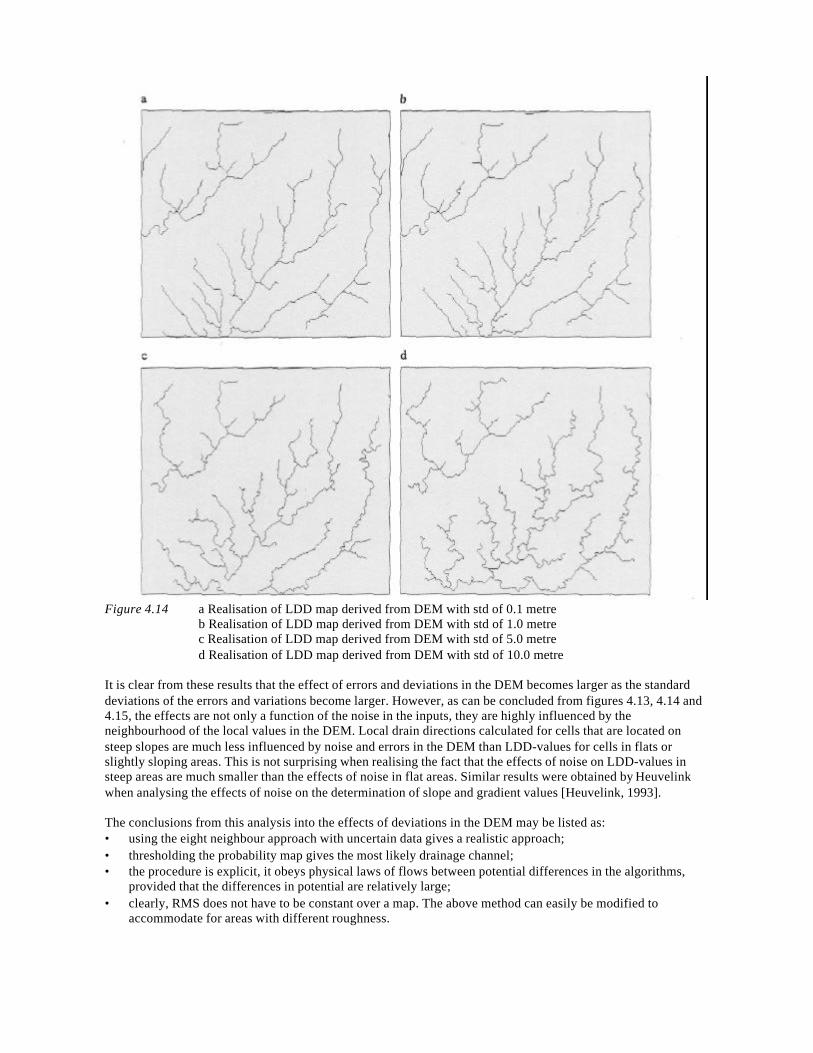
Figure 4.14 a Realisation of LDD map derived from DEM with std of 0.1 metreb Realisation of LDD map derived from DEM with std of 1.0 metrec Realisation of LDD map derived from DEM with std of 5.0 metred Realisation of LDD map derived from DEM with std of 10.0 metre

It is clear from these results that the effect of errors and deviations in the DEM becomes larger as the standarddeviations of the errors and variations become larger. However, as can be concluded from figures 4.13, 4.14 and4.15, the effects are not only a function of the noise in the inputs, they are highly influenced by theneighbourhood of the local values in the DEM. Local drain directions calculated for cells that are located onsteep slopes are much less influenced by noise and errors in the DEM than LDD-values for cells in flats orslightly sloping areas. This is not surprising when realising the fact that the effects of noise on LDD-values insteep areas are much smaller than the effects of noise in flat areas. Similar results were obtained by Heuvelinkwhen analysing the effects of noise on the determination of slope and gradient values [Heuvelink, 1993].

The conclusions from this analysis into the effects of deviations in the DEM may be listed as:• using the eight neighbour approach with uncertain data gives a realistic approach;• thresholding the probability map gives the most likely drainage channel;• the procedure is explicit, it obeys physical laws of flows between potential differences in the algorithms,

provided that the differences in potential are relatively large;• clearly, RMS does not have to be constant over a map. The above method can easily be modified to

accommodate for areas with different roughness.

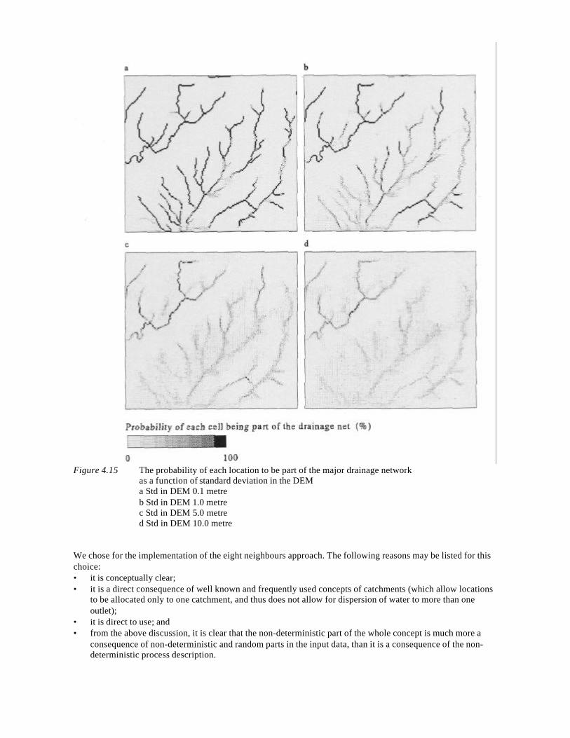
Figure 4.15 The probability of each location to be part of the major drainage networkas a function of standard deviation in the DEMa Std in DEM 0.1 metreb Std in DEM 1.0 metrec Std in DEM 5.0 metred Std in DEM 10.0 metre

We chose for the implementation of the eight neighbours approach. The following reasons may be listed for thischoice:• it is conceptually clear;• it is a direct consequence of well known and frequently used concepts of catchments (which allow locations

to be allocated only to one catchment, and thus does not allow for dispersion of water to more than oneoutlet);

• it is direct to use; and• from the above discussion, it is clear that the non-deterministic part of the whole concept is much more a

consequence of non-deterministic and random parts in the input data, than it is a consequence of the non-deterministic process description.

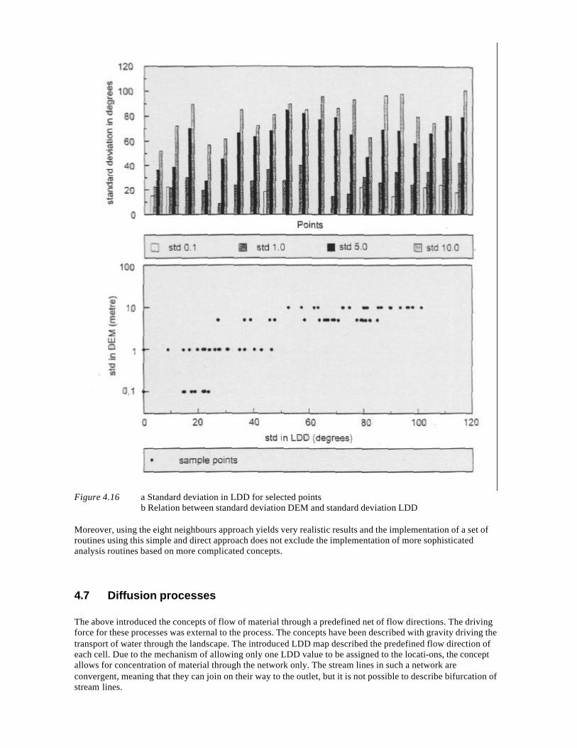
Figure 4.16 a Standard deviation in LDD for selected pointsb Relation between standard deviation DEM and standard deviation LDD

Moreover, using the eight neighbours approach yields very realistic results and the implementation of a set ofroutines using this simple and direct approach does not exclude the implementation of more sophisticatedanalysis routines based on more complicated concepts.

4.7 Diffusion processes

The above introduced the concepts of flow of material through a predefined net of flow directions. The drivingforce for these processes was external to the process. The concepts have been described with gravity driving thetransport of water through the landscape. The introduced LDD map described the predefined flow direction ofeach cell. Due to the mechanism of allowing only one LDD value to be assigned to the locati-ons, the conceptallows for concentration of material through the network only. The stream lines in such a network areconvergent, meaning that they can join on their way to the outlet, but it is not possible to describe bifurcation ofstream lines.

These concepts are sufficient to describe surface flow of water in rugged areas, but they fall short in situationswhere the driving force is not external to the process. Examples are groundwater and surface water in flat areas,for which the spatial distribution of the water itself is responsible for the distribution of the driving forces. Thebehaviour of the system aims at minimising the gradient in hydraulic head. These situations can be describedwith the diffusion process. In this process, it is the spatial distribution of the potential energy of the materialitself that provides the driving force for movement and transport.

A general formula for the diffusion process reads

Qx,y = -Dx,y grad(P) (4.12)

in whichQx,y = internal redistribution fluxDx,y = diffusion factorgrad(P) = components of the potential gradient

Jx = dP/dxJy = dP/dy

For the application of diffusion mechanisms in the mass balance concept, it is important to realise that thedriving force is not a function of the spatial distribution of the material, but of the spatial distribution of thepotential energy of this material. Therefore, the description of the diffusion process should include the relationbetween amount of mass and potential. This relation is described using some reference plane for which potentialis known and the storage capacity, which is defined as the increase in potential due to one unit increase in theamount of material. Simple cases may be described with linear (or linear approximations for) capacityparameters, but in complex cases this does not have to be satisfactory.

Diffusion processes are a function of a scalar field of potentials. This scalar field of potentials is described as afunction of amount in the storage compartment (the state variable) and the capacity of the storage compartment.Applying the diffuser operator yields two results: the new spatial distribution of mass in the storage compartmentand the internal redistribution fluxes due to this diffusion process. The internal fluxes are by definition lateralfluxes, which are stored in vectorfield variables.

Techniques to solve the diffusion process are known from groundwater hydrology and numerical algebra. Themost important techniques are based on finite difference and finite element algorithms [Bear and Verruyt, 1990]

The current version of the prototype PCRaster does not include the diffusor operators. The framework of thesystem, however, fully supports the mechanisms necessary for implementing these functions. Although not yetimplemented, the syntax of these diffusor operators with linear capacity coefficient would be something like:

<NewState>= diffusionstate(<StateMap>,<DiffusionFactor>,<StorageCapacityMap>)and

<InternalFlux> = diffusionflux(<StateMap>,<DiffusionFactor>,<StorageCapacityMap>).

Extended functionality has to be defined allowing for nonlinear storage capacity or situations with continuoussupply or withdrawal.

5 GENERIC MODELLING OF SURFACE HYDROLOGY ANDENVIRONMENTAL PROCESSES

"All these prepositions are empirical. It is not possible to prove them mathematically. In fact, it is a rathersimple matter to demonstrate by rational hydraulic analysis that not a single one of them is mathematically

accurate. Fortunately, nature is not aware of this."(Johnstone and Cross, 1949)

5.1 Introduction

Chapter 4 presented the concepts of mathematical modelling using discretised cells and explained the functionsand syntax of a wide range of generic tools for static and dynamic computations. That chapter extended well-known ideas of Map Algebra to cover aspects such as dynamic routing and flow, temporal change and iterationand presented them in the form of a mathematical spatial modelling language.

The aim of this chapter is to explain, with examples, how several prototypes of commonly used forms ofhydrological, hydraulic and environmental mathematical models can be programmed using the generic toolspresented in chapter 4. The object of the exercise is to demonstrate how steady state, lumped and dynamicmodels can be written in terms of the functionality that has been developed. Chapter 6 explains the application ofsome models to practical case studies, results are presented and critically evaluated.

In this chapter I have chosen to illustrate the use of the generic spatial modelling tools with models taken fromsurface water hydrology - soil water balance modelling, accumulation and concentration of water in catchments,point source and diffuse source pollutant dilution in streams, the determination of the Unit Hydrograph, dynamicsurface water routing and mass balance modelling of vegetation growth and competition. These provide a widerange of modelling approaches from empirical to physically-based models and from steady state conditions todynamic change.

There are many computer models which describe, with a varying degree of complexity, one or more componentsof the hydrologic cycle. The reader should note that this thesis does not attempt to derive new 'models' in thesense that the 'model' is a different mathematical formulation of a physical process. The models presented hereare 'new' because• they can use spatially distributed data, as included in the GIS; and• they can be programmed individually.

Therefor the user has full control over both the structure, the parameters and the spatial data. If the mathematicalformulation of the process is sensible, then the use of spatial generic tools should provide better results than byusing hardwired, lumped models.

Hydrologic modelling is concerned with the description of the water cycle, the flow of water and its constituentsover the land surface and in the subsurface. In general the total field of hydrology is divided into a set of morespecific elements, each describing a separate part of the hydrologic cycle. Also the processes of weather andclimate are intrinsic to the hydrologic cycle, but these processes tend to be covered by the fields of meteorologyand climatology, rather than by the discipline of hydrology. A more common view is that hydrology covers thepart of the hydrologic cycle where there is a close link between water, land and the biosphere.

Although hydrology is concerned with both surface water and ground water, the examples described here dealpredominantly with surface water. Surface water hydrology deals with the flow and distribution of water over thesurface of the earth. In large parts of the world, the most important control which affects surface flow istopography. There is a strong relation between channel distribution and topography, although in general onecannot treat topography as the only determining factor of surface runoff. Topography in its turn may be largelydetermined by surface flow through the processes of erosion and sedimentation.

Water balance studies describe the budget of water in a certain area (watershed or management unit). The sourceof water is precipitation, while losses occur as evapotranspiration, runoff at the outlet and subsurface flow toareas external to the study area. Major processes in this type of study are infiltration, evapotranspiration and

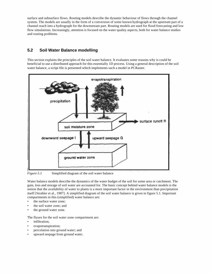
surface and subsurface flows. Routing models describe the dynamic behaviour of flows through the channelsystem. The models are usually in the form of a conversion of some known hydrograph at the upstream part of achannel reach into a hydrograph for the downstream part. Routing models are used for flood forecasting and lowflow simulations. Increasingly, attention is focused on the water quality aspects, both for water balance studiesand routing problems.

5.2 Soil Water Balance modelling

This section explains the principles of the soil water balance. It evaluates some reasons why is could bebeneficial to use a distributed approach for this essentially 1D process. Using a general description of the soilwater balance, a script file is presented which implements such a model in PCRaster.

Figure 5.1 Simplified diagram of the soil water balance

Water balance models describe the dynamics of the water budget of the soil for some area or catchment. Thegain, loss and storage of soil water are accounted for. The basic concept behind water balance models is thenotion that the availability of water to plants is a more important factor in the environment than precipitationitself [Strahler et al., 1987]. A simplified diagram of the soil water balance is given in figure 5.1. Importantcompartments in this (simplified) water balance are:• the surface water zone;• the soil water zone; and• the ground water zone.

The fluxes for the soil water zone compartment are:• infiltration;• evapotranspiration;• percolation into ground water; and• upward seepage from ground water.

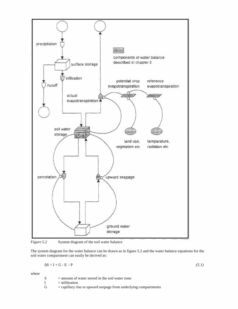
Figure 5.2 System diagram of the soil water balance

The system diagram for the water balance can be drawn as in figure 5.2 and the water balance equations for thesoil water compartment can easily be derived as:

∆S = I + G - E – P (5.1)

whereS = amount of water stored in the soil water zoneI = infiltrationG = capillary rise or upward seepage from underlying compartments

E = evapotranspirationP = percolation or downward seepage to underlying compartments

A common approach for the determination of the evapotranspiration rate is the distinction between potentialevapotranspiration, the water need for plants for a given meteorological regime, and the actualevapotranspiration, which is the water use of the plants in the given meteorological and soil moisture regime.Plants will suffer from water deficiency if soil moisture and precipitation are not sufficient to meet the need forwater expressed in the potential evapotranspiration [Strahler et al., 1987]. It is obvious that the actual flux fromthe soil water is not represented by the potential evapotranspiration but by the actual evapotranspiration.

Table 5.1 Meteorological input data for various methods of calculating ETrefMethod Rainfall Air

temperatureSolarradiation

Realtivehumidity

Wind speed Time step

Blaney andCriddle (1950)

+ month

Turc (1954) + + monthPenman(1948,1965)

+ + + + day

Thorntwaite-Mather (1957)

+ month

(Source: Feddes and Lenselink, 1994)

In general, the actual evapotranspiration rate of the soil is determined using a three step approach. In the firststep, the effects of climate and atmospheric conditions on evapotranspiration are determined, leading to anatmospheric evapotranspiration demand called the reference potential evapotranspiration ETref. This ETref isdefined as 'the rate of evapotranspiration from an extensive surface of 8 to 15 cm tall, green grass cover ofuniform height, actively growing, completely shading the ground and not short of water' [FAO, 1992]. Severalmethods are available for estimating this reference evapotranspiration. The characteristics of the major methodsare listed in table 5.1. The reference potential evapotranspiration rate could, in principle, be determined usingany of these evapotranspiration methods [Feddes and Lenselink, 1994]. In general, it can be stated that

ETref = f(climate, radiation, temperature, ...) (5.2)

The second step in the determination of the evapotranspiration rate is an adjustment of ETref for the effects ofcrop characteristics. One can relate an estimated reference potential evapotranspiration ETref to potential cropevapotranspiration ETpot for the crop under consideration by means of a crop coefficient

ETpot = kc * ETref (5.3)

whereETpot = potential crop evapotranspiration rate (mm/month)kc = crop coefficient (-)ETre f = reference potential evapotranspiration rate (mm/month)

The crop coefficient kc depends on characteristics of the vegetation, its development stage, growing season andthe prevailing weather conditions.

The third step in determining the evapotranspiration rate is the adjustment of the ETpot for soil water availability.Under limited soil water availability, actual evapotranspiration will be reduced. Such a limitation in availablesoil water occurs naturally if soil water, extracted from the root zone by evapotranspiration, is not replenished intime by rainfall or irrigation. Actual evapotranspiration ETact can be determined from the estimated potentialcrop evapotranspiration ETpot and the soil water balance. A general formulation of ETact is:

ETact = f (Sshortage, ETpot, ...) (5.4)

in whichSshortage = shortage in soil moisture

The maximum water storage capacity of the soil Smax is defined as the amount of water available in the soil forwater suppletion of crops. This is approximately the amount of water stored in the soil between the soil waterpressure at field capacity and the soil water pressure at wilting point [Groenendijk, 1989]. Smax is assumed to be

related to soil texture, and values for Smax can be derived from digitized soil texture maps using table 5.2 [Vander Leeden, 1990]. The shortage in soil moisture can now be defined as

Sshortage = Smax - Sact (5.5)

in whichSshortage = shortage in soil moistureSmax = maximum water storage capacitySact = actual water storage

Table 5.2 Soil types and maximum water storage capacity SmaxField capacity

[mm/m]Wilting point

[mm/m]Smax

[mm/m]Sand 100 25 75Loam 267 100 167Clay loam 317 150 167Clay 325 200 125(Source: Van der Leeden 1990 and U.S. Dept. of Agriculture)

To describe the model completely I introduce general terms for infiltration, percolation and upward seepage,formulated as

percolation = f(Sact, ...) (5.6)

upward seepage = f(Sact, ground water table, ...) (5.7)

infiltration = f(Sact, precipitation, ....) (5.8)

The important fluxes for the soil water balance are essentially vertical fluxes, and therefore soil water balancemodels are predominantly 1D models. However, several reasons may be listed for using a distributed approachfor this type of modelling:• spatial distributed water balance modelling allows for accounting the spatial variation in precipitation;• spatial distributed modelling allows for accounting the spatial distribution of radiation, temperature and

microclimate;• spatial distributed modelling can be advantageous for describing spatial variation in soil type and

characteristics;• spatial distributed modelling can be used for modelling the effects of slope and aspect on the soil water

balance; and• spatial distributed modelling allows for the evaluation of the effects of the crop characteristics of different

crops in the area.

The significance of the above reasons may vary with the spatial scale of the model. When applying soil waterbalances to small plots and fields, using time steps of hours or days, attention should be paid to spatial variationin temperature, radiation and precipitation due to slope, aspect and shading. In uneven terrain, there might be asignificant spatial variation in radiation and hours of sunshine. These effects can be accounted for using spatialdistributed maps of input data and model parameters. Maps with spatial distributed input data may beconstructed from Digital Elevation Models using algorithms for geomorphologic analysis [Evans, 1980; Horn,1981; Burrough, 1986]. Applying soil water balance models for large catchments or continental scale, using timesteps of months or even years, could mean that the spatial variation in crop characteristics, soil characteristics,temperature and precipitation may be considerable and should be accounted for [Kwadijk, 1993; Prentice et al.,1993].

The model can now be written as a script file:

# Soil Water Balance Modelling# Author: WPA van Deursen# Date: december 13, 1994binding

ModelArea = Area.map;CropType = Crops.map;

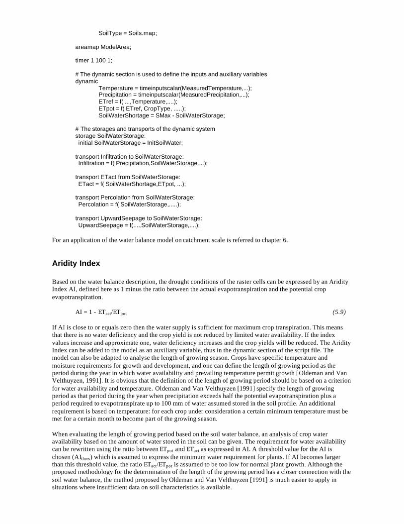
SoilType = Soils.map;

areamap ModelArea;

timer 1 100 1;

# The dynamic section is used to define the inputs and auxiliary variablesdynamic

Temperature = timeinputscalar(MeasuredTemperature,...);Precipitation = timeinputscalar(MeasuredPrecipitation,...);ETref = f( ...,Temperature,....);ETpot = f( ETref, CropType, .....);SoilWaterShortage = SMax - SoilWaterStorage;

# The storages and transports of the dynamic systemstorage SoilWaterStorage: initial SoilWaterStorage = InitSoilWater;

transport Infiltration to SoilWaterStorage: Infiltration = f( Precipitation,SoilWaterStorage....);

transport ETact from SoilWaterStorage: ETact = f( SoilWaterShortage,ETpot, ...);

transport Percolation from SoilWaterStorage: Percolation = f( SoilWaterStorage,.....);

transport UpwardSeepage to SoilWaterStorage: UpwardSeepage = f(....,SoilWaterStorage,....);

For an application of the water balance model on catchment scale is referred to chapter 6.

Aridity Index

Based on the water balance description, the drought conditions of the raster cells can be expressed by an AridityIndex AI, defined here as 1 minus the ratio between the actual evapotranspiration and the potential cropevapotranspiration.

AI = 1 - ETact/ETpot (5.9)

If AI is close to or equals zero then the water supply is sufficient for maximum crop transpiration. This meansthat there is no water deficiency and the crop yield is not reduced by limited water availability. If the indexvalues increase and approximate one, water deficiency increases and the crop yields will be reduced. The AridityIndex can be added to the model as an auxiliary variable, thus in the dynamic section of the script file. Themodel can also be adapted to analyse the length of growing season. Crops have specific temperature andmoisture requirements for growth and development, and one can define the length of growing period as theperiod during the year in which water availability and prevailing temperature permit growth [Oldeman and VanVelthuyzen, 1991]. It is obvious that the definition of the length of growing period should be based on a criterionfor water availability and temperature. Oldeman and Van Velthuyzen [1991] specify the length of growingperiod as that period during the year when precipitation exceeds half the potential evapotranspiration plus aperiod required to evapotranspirate up to 100 mm of water assumed stored in the soil profile. An additionalrequirement is based on temperature: for each crop under consideration a certain minimum temperature must bemet for a certain month to become part of the growing season.

When evaluating the length of growing period based on the soil water balance, an analysis of crop wateravailability based on the amount of water stored in the soil can be given. The requirement for water availabilitycan be rewritten using the ratio between ETpot and ETact as expressed in AI. A threshold value for the AI ischosen (AIthres) which is assumed to express the minimum water requirement for plants. If AI becomes largerthan this threshold value, the ratio ETact/ETpot is assumed to be too low for normal plant growth. Although theproposed methodology for the determination of the length of the growing period has a closer connection with thesoil water balance, the method proposed by Oldeman and Van Velthuyzen [1991] is much easier to apply insituations where insufficient data on soil characteristics is available.

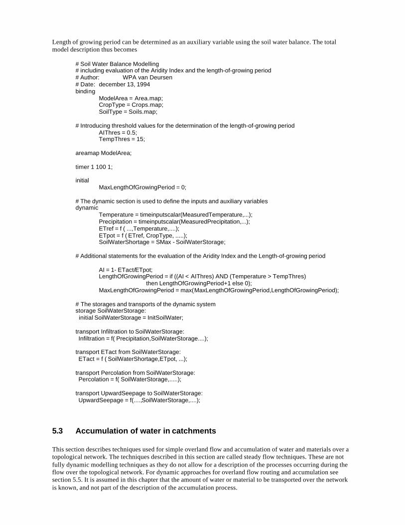
Length of growing period can be determined as an auxiliary variable using the soil water balance. The totalmodel description thus becomes

# Soil Water Balance Modelling# including evaluation of the Aridity Index and the length-of-growing period# Author: WPA van Deursen# Date: december 13, 1994binding

ModelArea = Area.map;CropType = Crops.map;SoilType = Soils.map;

# Introducing threshold values for the determination of the length-of-growing periodAIThres = 0.5;TempThres = 15;

areamap ModelArea;

timer 1 100 1;

initialMaxLengthOfGrowingPeriod = 0;

# The dynamic section is used to define the inputs and auxiliary variablesdynamic

Temperature = timeinputscalar(MeasuredTemperature,...);Precipitation = timeinputscalar(MeasuredPrecipitation,...);ETref = f ( ...,Temperature,....);ETpot = f ( ETref, CropType, .....);SoilWaterShortage = SMax - SoilWaterStorage;

# Additional statements for the evaluation of the Aridity Index and the Length-of-growing period

AI = 1- ETact/ETpot;LengthOfGrowingPeriod = if ((AI < AIThres) AND (Temperature > TempThres)

then LengthOfGrowingPeriod+1 else 0);MaxLengthOfGrowingPeriod = max(MaxLengthOfGrowingPeriod,LengthOfGrowingPeriod);

# The storages and transports of the dynamic systemstorage SoilWaterStorage: initial SoilWaterStorage = InitSoilWater;

transport Infiltration to SoilWaterStorage: Infiltration = f( Precipitation,SoilWaterStorage....);

transport ETact from SoilWaterStorage: ETact = f ( SoilWaterShortage,ETpot, ...);

transport Percolation from SoilWaterStorage: Percolation = f( SoilWaterStorage,.....);

transport UpwardSeepage to SoilWaterStorage: UpwardSeepage = f(....,SoilWaterStorage,....);

5.3 Accumulation of water in catchments

This section describes techniques used for simple overland flow and accumulation of water and materials over atopological network. The techniques described in this section are called steady flow techniques. These are notfully dynamic modelling techniques as they do not allow for a description of the processes occurring during theflow over the topological network. For dynamic approaches for overland flow routing and accumulation seesection 5.5. It is assumed in this chapter that the amount of water or material to be transported over the networkis known, and not part of the description of the accumulation process.

Simple accumulation of excess precipitation, surface water or other material over the LDD map introduced inchapter 4 is done with the function accu and associated functions. The use of the accu-functions in iterativemodelling assumes that all available water will discharge through the outlet within the same time step it becomesavailable. This steady flow approach is reasonable if the time step is long compared to the time of travel of waterthrough the channel network, and no information is needed on the timing of runoff events within the time step. Ifthe time step becomes smaller and approaches the order of magnitude of the travel time through the network, theuse of the accu-functions becomes less recommended. It is clear that now the assumption that all waterdischarges within the same time step becomes questionable, and the more advanced routing routines of section5.5 should be used.

The function accuflux operates on the LDD map to yield a map with on each grid cell the amount of water ormaterial that traversed this cell on its way to the outlet. The accompanying function accustate yields a mapcontaining the state of the system after accumulation of water. For each cell this map contains the amount ofwater that is not transported but left behind in the cell. As a consequence of the functionality of accu, accustateyields a map in which all water is accumulated in the pits of the catchment, since accu does not allow for anywater to stay behind during the lateral transport process. All cells not denoted as a pit or outlet thus contain avalue of zero. The function accustate has been added for consistency with the other accu related functions.

The accustate and accuflux functions do allow for additional water to be added to the transport network (lateralinflow into the channel), but they do not allow for any subtraction of water from the channel during the transportprocess. This implies that processes such as infiltration of upstream water in the river bed or evaporation fromthe river surface cannot be accounted for. If these processes become more important, the functions accuLTC,accuTT and accufraction are more appropriate. The application of these functions is discussed later in thissection.

Accuflux can be used for accumulation of all kinds of materials, as long as the above mentioned assumptions areaccepted as valid. Given the input of surface water (in the map SurfaceWater) to be accumulated through thetopological network (in the map LddMap) the function call is

StreamFlux = accuflux(LddMap,SurfaceWater);

I now introduce an example catchment with a topological network as given in figure 5.3a. Assuming a constantof 1 mm for SurfaceWater, the result of the accuflux function is given in figure 5.3b. Given a constant input of ahighly soluble pollutant that will not react or deposit on the bottom of the stream, the concentration of thepollutant in the stream can be determined by dividing the amount of pollutant transported through the system bythe amount of water flowing through the stream network. This yields the following script file fragment

StreamFlux = accuflux(LddMap, SurfaceWater);PollutantFlux = accuflux(LddMap,Pollutant);Concentration = PollutantFlux / StreamFlux;

Applying this script file to the results of the example catchment, and introducing a point source of this pollutant(figure 5.3c) yields a concentration map as given in figure 5.3d. Applying the script file to the situation in whichnon-point sources of the pollutant are distributed through the area as in figure 5.3e yields a stream concentrationas given in figure 5.3f.

Although useful as a first indication, attention should be paid to the fact that the assumptions underlying the accufunctions are very restrictive and real world situations will not meet these assumptions most of the time.

An improvement of the above is the introduction of losses during the transport process. As explained in chapter4, the process of transport and losses may be described as the result of four different mechanisms:• transport of the surplus occurs after a certain threshold of losses has been reached (function accuTT);• losses occur because transport capacity is limited (function accuLTC);• losses occur as a fraction of the material from upstream (function accufraction); and• massive transport of all the supplied material occurs once a certain threshold value has been exceeded

(function accutrigger).

Although these mechanisms are orthogonal, which means non of the mechanisms can be written as a function ofthe others, their use and results are similar. In this section, several applications of the use of these functions aregiven.

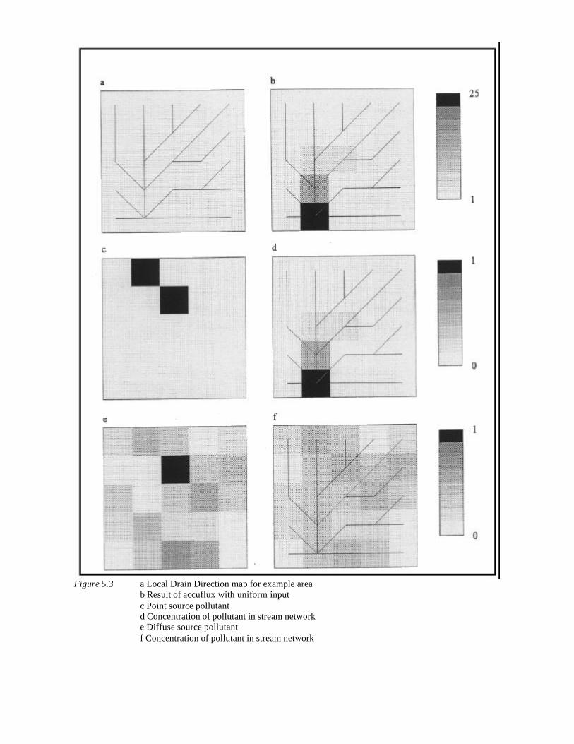
Figure 5.3 a Local Drain Direction map for example areab Result of accuflux with uniform inputc Point source pollutantd Concentration of pollutant in stream networke Diffuse source pollutantf Concentration of pollutant in stream network

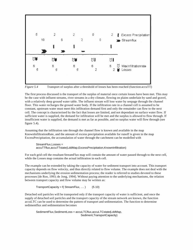
Figure 5.4 Transport of surplus after a threshold of losses has been reached (function accuTT)

The first process discussed is the transport of the surplus of material once certain losses have been met. This maybe the case with influent streams, river streams in a dry climate, flowing on plains underlain by sand and gravel,with a relatively deep ground water table. The influent stream will lose water by seepage through the channelfloor. This water recharges the ground water body. If the infiltration rate in a channel cell is assumed to beconstant, upstream water must meet this infiltration demand first and only the remainder can flow to the nextcell. The concept is characterised by the fact that losses are limited, and not dependant on surface water flow. Ifsufficient water is supplied, the demand for infiltration will be met and the surplus is allowed to flow through. Ifinsufficient water is supplied, the demand is met as far as possible, and no surplus water will flow through (seefigure 5.4).

Assuming that the infiltration rate through the channel flow is known and available in the mapKnownInfiltrationRate, and the amount of excess precipitation available for runoff is given in the mapExcessPrecipitation, the accumulation of water through the catchment can be modelled with

StreamFlux,Losses = accuTTflux,accuTTstate(LddMap,ExcessPrecipitation,KnownInfiltration)

For each grid cell the resultant StreamFlux map will contain the amount of water passed through to the next cell,while the Losses map contains the actual infiltration in each cell.

The example can be extended by taking the capacity of water for sediment transport into account. This transportcapacity depends on flow velocity, and thus directly related to flow volume. The example does not deal with themechanisms underlying the erosion sedimentation process; the reader is referred to studies devoted to theseprocesses [de Roo, 1993; de Jong, 1994]. Without paying attention to the underlying mechanisms, the relationbetween transport capacity and flow volume may be written as:

TransportCapacity = f( StreamFlux, .... ) (5.10)

Detached soil particles will be transported only if the transport capacity of water is sufficient, and once thesupply of detached soil particles and the transport capacity of the stream network are known, the functionaccuLTC can be used to determine the pattern of transport and sedimentation. The function to determinesedimentflux and sedimentation becomes

SedimentFlux,SedimentLoss = accuLTCflux,accuLTCstate(LddMap,Sediment,TransportCapacity)

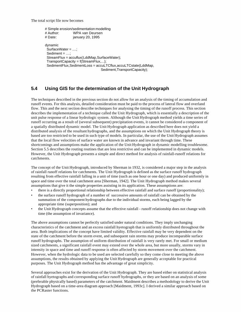
The total script file now becomes

# Simple erosion/sedimentation modelling# Author: WPA van Deursen# Date: january 20, 1995

dynamic SurfaceWater = ....; Sediment = ....; StreamFlux = accuflux(LddMap,SurfaceWater); TransportCapacity = f(StreamFlux,...); SedimentFlux,SedimentLoss = accuLTCflux,accuLTCstate(LddMap,

Sediment,TransportCapacity);

5.4 Using GIS for the determination of the Unit Hydrograph

The techniques described in the previous section do not allow for an analysis of the timing of accumulation andrunoff events. For this analysis, detailed consideration must be paid to the process of lateral flow and overlandflow. This and the next section describe techniques for analysing the timing of the runoff process. This sectiondescribes the implementation of a technique called the Unit Hydrograph, which is essentially a description of theunit pulse response of a linear hydrologic system. Although the Unit Hydrograph method yields a time series ofrunoff occurring as a result of (several subsequent) precipitation events, it cannot be considered a component ofa spatially distributed dynamic model. The Unit Hydrograph application as described here does not yield adistributed analysis of the resultant hydrographs, and the assumptions on which the Unit Hydrograph theory isbased are too restricted to be used in such type of models. In particular, the use of the Unit Hydrograph assumesthat the local flow velocities of surface water are known in advance and invariant through time. Theseshortcomings and assumptions make the application of the Unit Hydrograph in dynamic modelling troublesome.Section 5.5 describes the routing routines that are less restrictive and can be implemented in dynamic models.However, the Unit Hydrograph presents a simple and direct method for analysis of rainfall-runoff relations forcatchments.

The concept of the Unit Hydrograph, introduced by Sherman in 1932, is considered a major step in the analysisof rainfall runoff relations for catchments. The Unit Hydrograph is defined as the surface runoff hydrographresulting from effective rainfall falling in a unit of time (such as one hour or one day) and produced uniformly inspace and time over the total catchment area [Sherman, 1942]. The Unit Hydrograph method makes severalassumptions that give it the simple properties assisting in its application. These assumptions are:• there is a directly proportional relationship between effective rainfall and surface runoff (proportionality);• the surface runoff hydrograph of a number of successive amounts of rainfall can be obtained by the

summation of the component hydrographs due to the individual storms, each being lagged by theappropriate time (superposition); and

• the Unit Hydrograph concepts assume that the effective rainfall - runoff relationship does not change withtime (the assumption of invariance).

The above assumptions cannot be perfectly satisfied under natural conditions. They imply unchangingcharacteristics of the catchment and an excess rainfall hyetograph that is uniformly distributed throughout thearea. Both implications of the concept have limited validity. Effective rainfall may be very dependent on thestate of the catchment before the storm event, and subsequent rain storms may produce incomparable surfacerunoff hydrographs. The assumption of uniform distribution of rainfall is very rarely met. For small or mediumsized catchments, a significant rainfall event may extend over the whole area, but more usually, storms vary inintensity in space and time and runoff response is often affected by storm movement over the catchment.However, when the hydrologic data to be used are selected carefully so they come close to meeting the aboveassumptions, the results obtained by applying the Unit Hydrograph are generally acceptable for practicalpurposes. The Unit Hydrograph method has the advantage of great simplicity.

Several approaches exist for the derivation of the Unit Hydrograph. They are based either on statistical analysisof rainfall hyetographs and corresponding surface runoff hydrographs, or they are based on an analysis of some(preferable physically based) parameters of the catchment. Maidment describes a methodology to derive the UnitHydrograph based on a time-area diagram approach [Maidment, 1993c]. I derived a similar approach based onthe PCRaster functions.

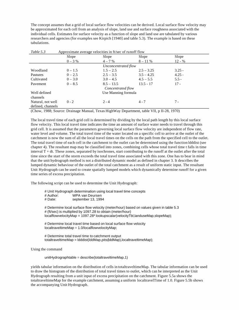
The concept assumes that a grid of local surface flow velocities can be derived. Local surface flow velocity maybe approximated for each cell from an analysis of slope, land use and surface roughness associated with theindividual cells. Estimates for surface velocity as a function of slope and land use are tabulated by variousresearchers and agencies (for examples see Kirpich [1940] and table 5.3). The example is based on thesetabulations.

Table 5.3 Approximate average velocities in ft/sec of runoff flowSlope0 – 3 %

Slope4 – 7 %

Slope8 – 11 %

Slope12 - %

Unconcentrated flowWoodland 0 – 1.5 1.5 – 2.5 2.5 – 3.25 3.25 -Pastures 0 – 2.5 2.5 – 3.5 3.5 – 4.25 4.25 -Cultivated 0 – 3.0 3.0 – 4.5 4.5 – 5.5 5.5 -Pavement 0 – 8.5 8.5 – 13.5 13.5 - 17 17 -

Concentrated flowWell definedchannels

Use Manning formula

Natural, not welldefined, channels

0 - 2 2 - 4 4 - 7 7 -

(Chow, 1988; Source: Drainage Manual, Texas HighWay Department, table VII, p II-28, 1970)

The local travel time of each grid cell is determined by dividing by the local path length by this local surfaceflow velocity. This local travel time indicates the time an amount of surface water needs to travel through thisgrid cell. It is assumed that the parameters governing local surface flow velocity are independent of flow rate,water level and volume. The total travel time of the water located on a specific cell to arrive at the outlet of thecatchment is now the sum of all the local travel times on the cells on the path from the specified cell to the outlet.The total travel time of each cell in the catchment to the outlet can be determined using the function ldddist (seechapter 4). The resultant map may be classified into zones, combining cells whose total travel time t falls in timeinterval T + dt. These zones, separated by isochrones, start contributing to the runoff at the outlet after the totaltime since the start of the storm exceeds the total travel time associated with this zone. One has to bear in mindthat the unit hydrograph method is not a distributed dynamic model as defined in chapter 3. It describes thelumped dynamic behaviour of the outlet of the total catchment as a result of uniform static input. The resultantUnit Hydrograph can be used to create spatially lumped models which dynamically determine runoff for a giventime series of excess precipitation.

The following script can be used to determine the Unit Hydrograph:

# Unit Hydrograph determination using local travel time concepts# Author: WPA van Deursen# Date: september 13, 1994

# Determine local surface flow velocity (meter/hour) based on values given in table 5.3# (ft/sec) is multiplied by 1097.28 to obtain (meter/hour)localflowvelocityMap = 1097.28* lookupscalar(velocityTbl,landuseMap,slopeMap);

# Determine local travel time based on local surface flow velocitylocaltraveltimeMap = 1.0/localflowvelocityMap;

# Determine total travel time to catchment outputtotaltraveltimeMap = ldddist(lddMap,pits(lddMap),localtraveltimeMap);

Using the command

unitHydrographtable = describe(totaltraveltimeMap,1)

yields tabular information on the distribution of cells in totaltraveltimeMap. The tabular information can be usedto draw the histogram of the distribution of total travel times to outlet, which can be interpreted as the UnitHydrograph resulting from a unit input of excess precipitation on the catchment. Figure 5.5a shows thetotaltraveltimeMap for the example catchment, assuming a uniform localtravelTime of 1.0. Figure 5.5b showsthe accompanying Unit Hydrograph.

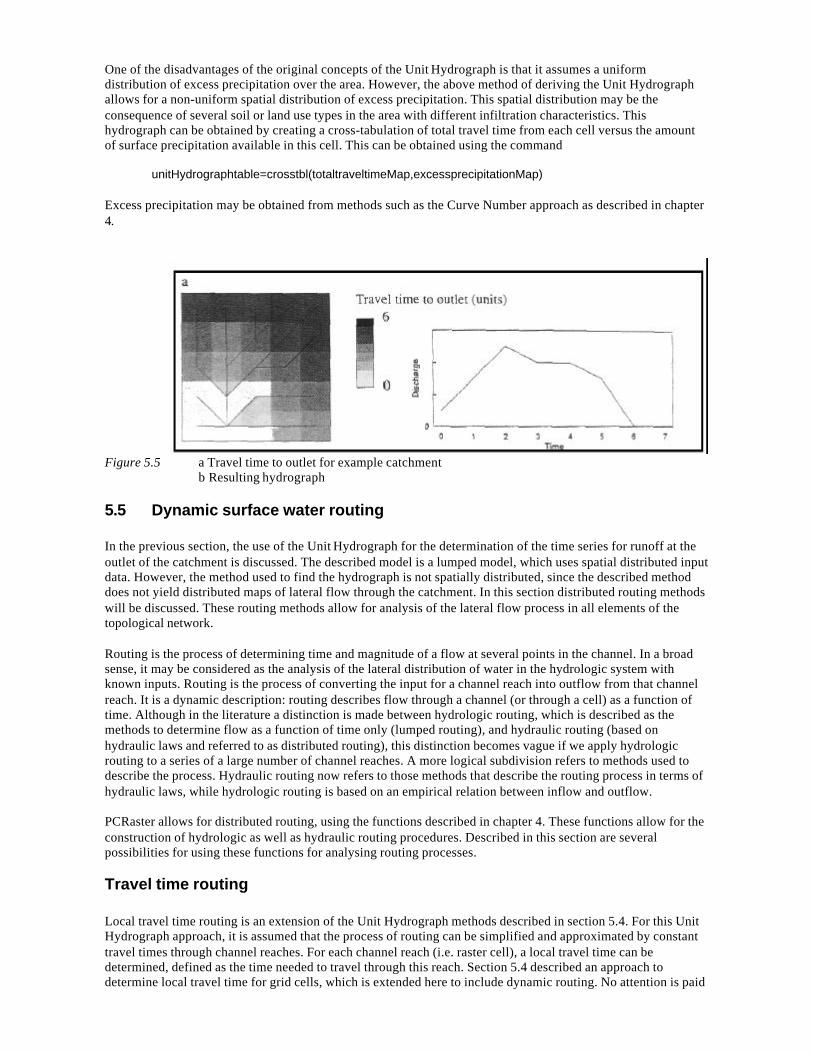
One of the disadvantages of the original concepts of the Unit Hydrograph is that it assumes a uniformdistribution of excess precipitation over the area. However, the above method of deriving the Unit Hydrographallows for a non-uniform spatial distribution of excess precipitation. This spatial distribution may be theconsequence of several soil or land use types in the area with different infiltration characteristics. Thishydrograph can be obtained by creating a cross-tabulation of total travel time from each cell versus the amountof surface precipitation available in this cell. This can be obtained using the command

unitHydrographtable=crosstbl(totaltraveltimeMap,excessprecipitationMap)

Excess precipitation may be obtained from methods such as the Curve Number approach as described in chapter4.

Figure 5.5 a Travel time to outlet for example catchmentb Resulting hydrograph

5.5 Dynamic surface water routing

In the previous section, the use of the Unit Hydrograph for the determination of the time series for runoff at theoutlet of the catchment is discussed. The described model is a lumped model, which uses spatial distributed inputdata. However, the method used to find the hydrograph is not spatially distributed, since the described methoddoes not yield distributed maps of lateral flow through the catchment. In this section distributed routing methodswill be discussed. These routing methods allow for analysis of the lateral flow process in all elements of thetopological network.

Routing is the process of determining time and magnitude of a flow at several points in the channel. In a broadsense, it may be considered as the analysis of the lateral distribution of water in the hydrologic system withknown inputs. Routing is the process of converting the input for a channel reach into outflow from that channelreach. It is a dynamic description: routing describes flow through a channel (or through a cell) as a function oftime. Although in the literature a distinction is made between hydrologic routing, which is described as themethods to determine flow as a function of time only (lumped routing), and hydraulic routing (based onhydraulic laws and referred to as distributed routing), this distinction becomes vague if we apply hydrologicrouting to a series of a large number of channel reaches. A more logical subdivision refers to methods used todescribe the process. Hydraulic routing now refers to those methods that describe the routing process in terms ofhydraulic laws, while hydrologic routing is based on an empirical relation between inflow and outflow.

PCRaster allows for distributed routing, using the functions described in chapter 4. These functions allow for theconstruction of hydrologic as well as hydraulic routing procedures. Described in this section are severalpossibilities for using these functions for analysing routing processes.

Travel time routing

Local travel time routing is an extension of the Unit Hydrograph methods described in section 5.4. For this UnitHydrograph approach, it is assumed that the process of routing can be simplified and approximated by constanttravel times through channel reaches. For each channel reach (i.e. raster cell), a local travel time can bedetermined, defined as the time needed to travel through this reach. Section 5.4 described an approach todetermine local travel time for grid cells, which is extended here to include dynamic routing. No attention is paid

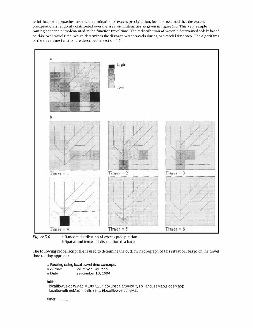
to infiltration approaches and the determination of excess precipitation, but it is assumed that the excessprecipitation is randomly distributed over the area with intensities as given in figure 5.6. This very simplerouting concept is implemented in the function traveltime. The redistribution of water is determined solely basedon this local travel time, which determines the distance water travels during one model time step. The algorithmsof the traveltime function are described in section 4.5.

Figure 5.6 a Random distribution of excess precipitationb Spatial and temporal distribution discharge

The following model script file is used to determine the outflow hydrograph of this situation, based on the traveltime routing approach.

# Routing using local travel time concepts# Author: WPA van Deursen# Date: september 13, 1994

initial localflowvelocityMap = 1097.28* lookupscalar(velocityTbl,landuseMap,slopeMap); localtraveltimeMap = cellsize(....)/localflowvelocityMap;

timer ...........

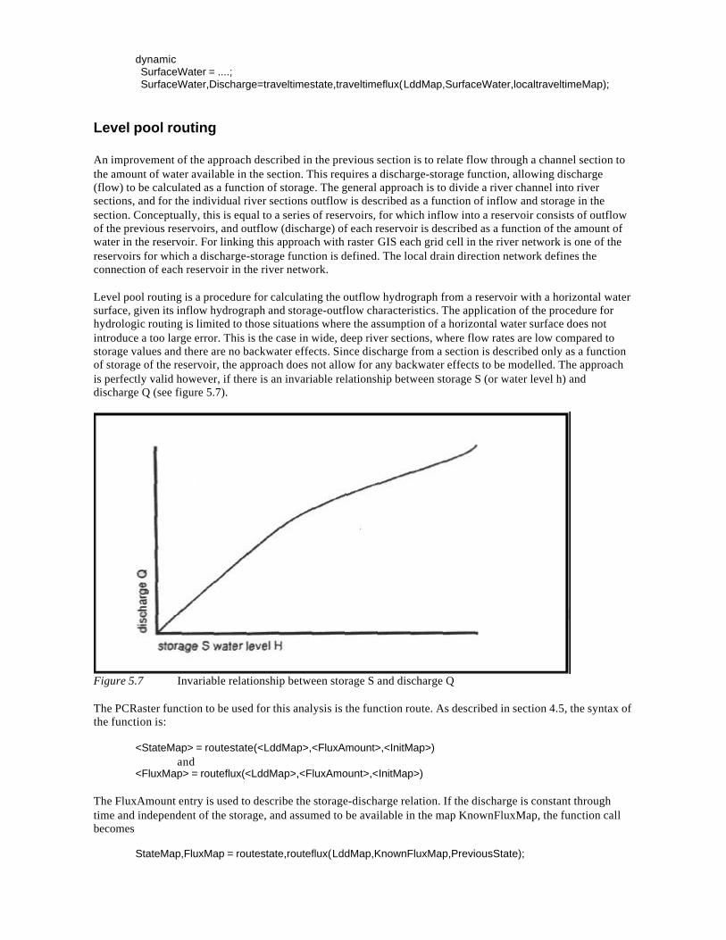
dynamic SurfaceWater = ....; SurfaceWater,Discharge=traveltimestate,traveltimeflux(LddMap,SurfaceWater,localtraveltimeMap);

Level pool routing

An improvement of the approach described in the previous section is to relate flow through a channel section tothe amount of water available in the section. This requires a discharge-storage function, allowing discharge(flow) to be calculated as a function of storage. The general approach is to divide a river channel into riversections, and for the individual river sections outflow is described as a function of inflow and storage in thesection. Conceptually, this is equal to a series of reservoirs, for which inflow into a reservoir consists of outflowof the previous reservoirs, and outflow (discharge) of each reservoir is described as a function of the amount ofwater in the reservoir. For linking this approach with raster GIS each grid cell in the river network is one of thereservoirs for which a discharge-storage function is defined. The local drain direction network defines theconnection of each reservoir in the river network.

Level pool routing is a procedure for calculating the outflow hydrograph from a reservoir with a horizontal watersurface, given its inflow hydrograph and storage-outflow characteristics. The application of the procedure forhydrologic routing is limited to those situations where the assumption of a horizontal water surface does notintroduce a too large error. This is the case in wide, deep river sections, where flow rates are low compared tostorage values and there are no backwater effects. Since discharge from a section is described only as a functionof storage of the reservoir, the approach does not allow for any backwater effects to be modelled. The approachis perfectly valid however, if there is an invariable relationship between storage S (or water level h) anddischarge Q (see figure 5.7).

Figure 5.7 Invariable relationship between storage S and discharge Q

The PCRaster function to be used for this analysis is the function route. As described in section 4.5, the syntax ofthe function is:

<StateMap> = routestate(<LddMap>,<FluxAmount>,<InitMap>)and

<FluxMap> = routeflux(<LddMap>,<FluxAmount>,<InitMap>)

The FluxAmount entry is used to describe the storage-discharge relation. If the discharge is constant throughtime and independent of the storage, and assumed to be available in the map KnownFluxMap, the function callbecomes

StateMap,FluxMap = routestate,routeflux(LddMap,KnownFluxMap,PreviousState);

withStateMap = resulting map with the state (amount stored in each grid cell)FluxMap = resulting map with the calculated fluxLddMap = input local drain direction map containing the river networkKnownFluxMap = input flux map with known (constant) fluxPreviousState = input state map.

As explained in section 4.5.4, the function route evaluates the KnownFlux entry, and calculates the flux based onthis entry. In the case of constant discharge, where the amount of water stored in the grid cell is sufficient tosatisfy this flux, the resultant FluxMap will contain the same values as the KnownFluxMap. If the amount storedin the system is insufficient to satisfy this flux, the resultant FluxMap will contain the amount of discharge thestorage was capable to supply. Dynamic behaviour of this routing procedure can be evaluated by assigning theresultant map to be input for the next time step, thus yielding a script file similar to

# Routing example 1# Dynamic routing using constant (predetermined) fluxes# Author: WPA van Deursen# Date: september 28, 1994

bindingModelArea = area.map;KnownFluxMap = constantflux.map;InitStateMap = initstate.map;LddMap = ldd.map;Stations = stations.map;Discharge = discharge.dat;

areamap ModelArea;

timer 1 10 1;

initialState = InitStateMap;

dynamic# allowing for additional water to be added to the routing processState = State + ......# routing of waterState,Flux=routestate,routeflux(LddMap,KnownFluxMap,State)# writing results for selected pointsreport Discharge = timeoutput(Stations,Flux);

A storage-discharge behaviour (where discharge is a function of storage) may be constructed by replacing theconstant KnownFlux with a relation describing flux as a function of storage. Assuming a known relation betweenstorage and discharge given by the relation

Q = aSb (5.11)

with known values for a and b, the function call becomes

StateMap,FluxMap = routestate,routeflux(LddMap, a*StateMap^b, StateMap);

withStateMap = map with the state of the systemFluxMap = resulting map with the calculated fluxLddMap = input local drain direction map containing the river networka,b = (spatial distributed) constants

and the script file for dynamic modelling becomes

# Routing example 2# Dynamic routing using invariable storage-discharge relation# Author: WPA van Deursen# Date: september 28, 1994

bindingModelArea = area.map;InitStateMap = initstate.map;LddMap = ldd.map;Stations = stations.map;Discharge = discharge.dat;a = ....b = ....

areamap ModelArea;

timer 1 10 1;

initialState = InitStateMap;

dynamic# allowing for additional water to be added to the routing processState = State + ......# routing of waterState,Flux=routestate,routeflux(LddMap,a*State^b,State);# writing results for selected pointsreport Discharge = timeoutput(Stations,Flux);

The storage-discharge relation can also be used to construct water level-discharge relations, which mightrepresent Q-h rating curves for river sections. Assuming a rectangular cross section through the channel, waterlevel is a linear function of storage

h = c * S (5.12)

A linear reservoir with discharge as a linear function of water level (Q = k * h) can thus be constructed bycombining the two relations, yielding

Q = k * h = k * c * S. (5.13)

This function can be used for level pool routing through a rectangular channel, assuming a linear relationbetween water level and discharge, using the route-function

State,Flux = routestate,routeflux(LddMap,k * c * State,State)

If the relation between channel reach storage and water level cannot be written as a formula, or the formulabecomes too complex, the lookuptable function can be used. The function call becomes

State,Flux= routestate,routeflux(LddMap,k * lookupscalar(leveltable,State),State)

This approach may be very useful when dealing with situations where runoff has to be routed through a channelwith floodplains. The relation between water level and channel reach storage cannot be written as a simplecontinuous function, and a superior approach may be to construct a table relating water level to channel storage.

# Routing example 3# Dynamic routing using a level pool approach for channel reaches with floodplains# Author: WPA van Deursen# Date: september 28, 1994

bindingModelArea = area.map;InitStateMap = initstate.map;LddMap = ldd.map;Waterlevel = waterlevel.tbl;Stations = stations.map;Discharge = discharge.dat;k = ....

areamap ModelArea;

timer 1 10 1;

initialState = InitStateMap;

dynamic# allowing for additional water to be added to the routing processState = State + ......# routing of waterState,Flux = routestate,routeflux(LddMap,k*lookupscalar(Waterlevel,State),State);# writing results for selected pointsreport Discharge = timeoutput(Stations,Flux);

5.6 Advective transport, erosion and sedimentation

The route operators can be used to model processes of trans-port. Using these operators, the equations describingthe transport mechanisms are defined by the user. If the trans-port equations are written as a function of anotherrouting process, these operators can be used to implement advective transport.

Advective transport can be defined as transport of material where a carrier flux is responsible for the transportingmechanism. Examples from physical geography are the transport of pollutants driven by water movement, butalso the transport of sediment by water flow. As described in the previous sections, this movement of water canbe described with the route-functions as

CarrierState,CarrierFlux = routestate,route-flux(LddMap,.....,CarrierState)

in which the transport equations for water can be included.

The transport of a pollutant (or sediment) as an effect of this water movement can be written as

Transport of pollutant = f(CarrierFlux,...) (5.14)

The combined definition of transport of water and pollutant is implemented with

CarrierState,CarrierFlux = routestate,route-flux(LddMap,.......,CarrierState);PollutantState,PollutantFlux = routestate,routeflux(LddMap,f(CarrierFlux,...),PollutantState);

A simple example of the transport of salt dissolved in water can be simulated based on the concentration of saltin the carrier. The transport of salt can be simulated as moving the amount of water with the dissolved salt (ofknown concentra-tion) from one cell to the next. The following script file implements this mechanism.

CarrierState = .....;PollutantState = .....;Concentration = PollutantState/CarrierState;CarrierState,CarrierFlux = routestate,route-flux(Lddmap,....,CarrierState);PollutantState,PollutantFlux =routestate,routeflux(LddMap,

CarrierFlux*Concentrati-on,PollutantState);

The amount of salt transported is described as the concentra-tion of salt multiplied by the amount of watertransported. The state of the salt component is determined as the result of moving this amount of salt through theLDD map.

5.7 Environmental modelling

The techniques described in the previous section can also be used for modelling other environmental processes.This section is devoted to ecological and environmental models. Here I focus only on processes of vegetationgrowth, competition and dispersal. Although it is clear that there are many more interesting processes in

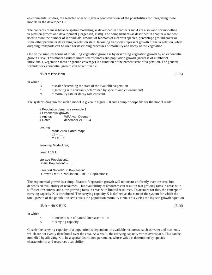
environmental studies, the selected ones will give a good overview of the possibilities for integrating thesemodels in the developed GIS.

The concepts of mass balance spatial modelling as developed in chapter 3 and 4 are also valid for modellingvegetation growth and development [Jørgensen, 1988]. The compartments as described in chapter 4 are nowused to store the number of individuals, amount of biomass of a certain species, percentage ground cover orsome other parameter describing vegetation state. Incoming transports represent growth of the vegetation, whileoutgoing transports can be used for describing processes of mortality and decay of the vegetation.

One of the simplest forms of modelling vegetation growth is by describing vegetation growth by an exponentialgrowth curve. This model assumes unlimited resources and population growth (increase of number ofindividuals, vegetation mass or ground coverage) is a function of the present state of vegetation. The generalformula for exponential growth can be written as:

dB/dt = B*c-B*m (5.15)

in whichB = scalar describing the state of the available vegetationc = growing rate constant (determined by species and environment)m = mortality rate or decay rate constant.

The systems diagram for such a model is given in figure 5.8 and a simple script file for the model reads:

# Population dynamics example 1# Exponential growth# Author: WPA van Deursen# Date: december 21, 1994

bindingModelArea = area.map;c1 = ....;m1 = ....;

areamap ModelArea;

timer 1 10 1;

storage Population1; initial Population1 = ....;

transport Growth1 to Population1: Growth1 = c1 * Population1 - m1 * Population1;

The exponential growth is a simplification. Vegetation growth will not occur uniformly over the area, butdepends on availability of resources. This availability of resources can result in fast growing rates in areas withsufficient resources, and slow growing rates in areas with limited resources. To account for this, the concept ofcarrying capacity K is introduced. The carrying capacity K is defined as the state of the system for which thetotal growth of the population B*c equals the population mortality B*m. This yields the logistic growth equation

dB/dt = rB(K-B)/K (5.16)

in whichr = intrinsic rate of natural increase = c - mK = carrying capacity.

Clearly the carrying capacity of a population is dependent on available resources, such as water and nutrients,which are not evenly distributed over the area. As a result, the carrying capacity varies over space. This can bemodelled by allowing K to be a spatial distributed parameter, whose value is determined by speciescharacteristics and resources availability.

Figure 5.8 System diagram of simple ecologic model

Logistic growth can be the consequence of external factors, but typically growth is restricted because thevegetation is competing for a limited amount of resources. Both individuals of the same species and individualsof different species have to compete for the same limited amount of resources. The limited resources mayinclude water and nutrients, but one of the major competition processes is competition for light. As vegetationgrows, it develops a larger surface of leaves for intercepting light, thus creating a larger capability for growthand maintenance. However, this larger surface of leaves will shadow underlying leaves, and these leaves will nolonger take part in the production of biomass. Other species developing in the neighbourhood of the plant willalso attempt to grow large surfaces for intercepting light, and as these neighbours all develop, combined theywill intercept almost all available light. The development of a certain individual will yield a relative advantagefor this individual over other species in the capability of intercepting light, but at the same time it leads to asituation in which less of the same resource is available to be intercepted. The growth process for twopopulations in which a simple description of competition for limited resources is implemented reads:

dB1/dt = r1 * B1 * (K1 - B1 - α12B2)/K1 (5.17)and

dB2/dt = r2 * B2 * (K2 - B2 - α21B1)/K2

whereα12 and α21 are competition coefficients

This yields the following script file

# Population dynamics example 2# Population competition# Author: WPA van Deursen# Date: december 21, 1994

bindingModelArea = area.map;K1Map = K1.map;K2Map = K2.map;r1 = ....;r2 = ....;alpha12 = ....;alpha21 = ....;

areamap ModelArea;

timer 1 100 1;

storage Population1;

initial Population1 = 0.1;

storage Population2; initial Population2 = 0.1;

transport Growth1 to Population1: Growth1 = r1 * Population1 * (K1Map - Population1 - alpha12 * Population2)/K1Map;

transport Growth2 to Population2: Growth2 = r2 * Population2 * (K2Map - Population2 - alpha21 * Population1)/K2Map;

In the above examples, a certain initial amount of biomass is available, and it is assumed that the process ofvegetation growth is initiated with this amount. If the initial amount of a certain vegetation at a certain location is0, or if all of the vegetation at a certain location has died off, the above model descriptions do not allow forspontaneous rise of new individuals to initiate the growth process. Some process of dispersion of the populationthrough the area has to be incorporated to allow for colonization of locations previously not occupied.Applicable dispersion processes are seed distribution, clonal growth or vegetative reproduction. The followingscript introduces seed distribution as a random process to occupy empty regions. The amount of seed found at alocation may be modelled as a function of (the inverse of) the distance to other locations occupied by the samespecies. For each location, the distance to the nearest location occupied by the species may be found using thespread function, and a general formulation of seed distribution may be

Seed = f (...., spread(Population1, ..., ...), ...) (5.18)

Some threshold of population state may be introduced, indicating that populations are only productive after acertain maturation.

Seed = f (..., spread(Population1 gt 0.5, ...., ....), ....) (5.19)

The growth of each population is now a combination of germination of seed and the growth as described in theprevious example. The script file to implement this process is

# Population dynamics example 3# Population competition and seed distribution# Author: WPA van Deursen# Date: december 21, 1994

bindingModelArea = area.map;K1Map = K1.map;K2Map = K2.map;r1 = ....;r2 = ....;alpha12 = ....;alpha21 = ....;Thres1 = ....;Thres2 = ....;

areamap ModelArea;

timer 1 100 1;

dynamicseed1 = ...... spread(Population1 gt Thres1, ....., .....).....;seed2 = ...... spread(Population2 gt Thres2, ....., .....).....;

storage Population1; initial Population1 = 0.1;

storage Population2; initial Population2 = 0.1;

transport Growth1 to Population1: Growth1 = r1 * Population1 * (K1Map - Population1 - alpha12 * Population2)/

K1Map + ..... seed1....;

transport Growth2 to Population2: Growth2 = r2 * Population2 * (K2Map - Population2 - alpha21 * Population1)/

K2Map + .... seed2....;

The dispersion of seed can be modelled with other tools as well. If a predominant wind direction is responsiblefor dispersion into one direction, a LDD-map may be constructed as a preferred direction of seed dispersal. Theaccu and route functions are now available to describe the seed dispersal as a consequence of wind from a majordirection. The same approach may be used for modelling catastrophic events such as forest fire, which is spreadinto the direction of the wind only.

6 CASE STUDIES

6.1 Introduction

This chapter presents several applications based on the PCRaster-software that have been developed over the lastfive years. My major objective in this research was not to build and test hydrological and ecological models, butas the development of the software progressed, the need for testing using more extended applications emerged.In this chapter, I want to illustrate the use and robustness of the PCRaster tools. The descriptions in this chapterare not meant to verify the validity of the results, and reference is made to the other publications on the models.It is through the processes of cooperation and mutual influence that both the PCRaster software and theseapplication-projects got their final shape.

In this chapter the prototypes and techniques described in the previous chapters have been incorporated intosimulation models for hydrological and ecological purposes. Section 6.2 deals with the development andapplication of catchment scale water balance models used to analyse the sensitivity of the hydrologic regime oflarge river basins to climate change. These models, the RHINEFLOW class of PCRaster models, incorporate thesoil water balance model and the steady flow accumulation of surface runoff as described in chapter 5. TheRHINEFLOW model was used to investigate the effects of possible climate changes in the Rhine basin on thedischarge of the river Rhine. A modified version of these models, the GBP model, incorporates the analysis ofdrought conditions by the aridity index described in section 5.2. This model was used for climate changeresearch on the Ganges-Brahmaputra basin.

Section 6.3 describes the development of an ecological simulation model. This PCRaster model, named CalGIS,simulates the competition between heather (Calluna) and grass (Deschampsia). The CalGIS model uses the massbalance approach for vegetation development. This model incorporates the inter-species competition modeldescribed in section 5.7. A disease in the heather population is introduced, which infects individuals randomlyand contaminates the area in the neighbourhood of the infected locations, using the prototypes introduced insection 5.7.

The study concerning the Rhine catchment is published in Kwadijk [1993] and as CHR/KHR report [CHR/KHR,1995]. The Ganges-Brahmaputra study has been published as a Resource Analysis project report [ResourceAnalysis, 1994]. The research for the water balances was carried out in cooperation with Jaap Kwadijk of theFaculty of Physical Geography, University of Utrecht.

The presentation of the research for the Calluna model has been modified from the publication 'Analysis ofheathland dynamics using a spatial distributed GIS model' [Van Deursen and Heil, 1993]. This part of the studywas carried out in cooperation with Gerrit Heil, currently working at Resource Analysis, Delft and the Universityof Utrecht.

6.2 Water balance studies of large river basins with respect to theirsensitivity to climate changes

6.2.1 Introduction

The world climate is expected to react to the enhanced green-house effect with changed patterns of precipitationand temperature distribution in time and space. Consequently, streamflow is also expected to change in volumeand distribution over the year, giving major concerns to policy makers who are concerned with drought andflooding. Long-term strategies for future river manage-ment require quantitative information on these changes,for which hydrological models can often be important tools.

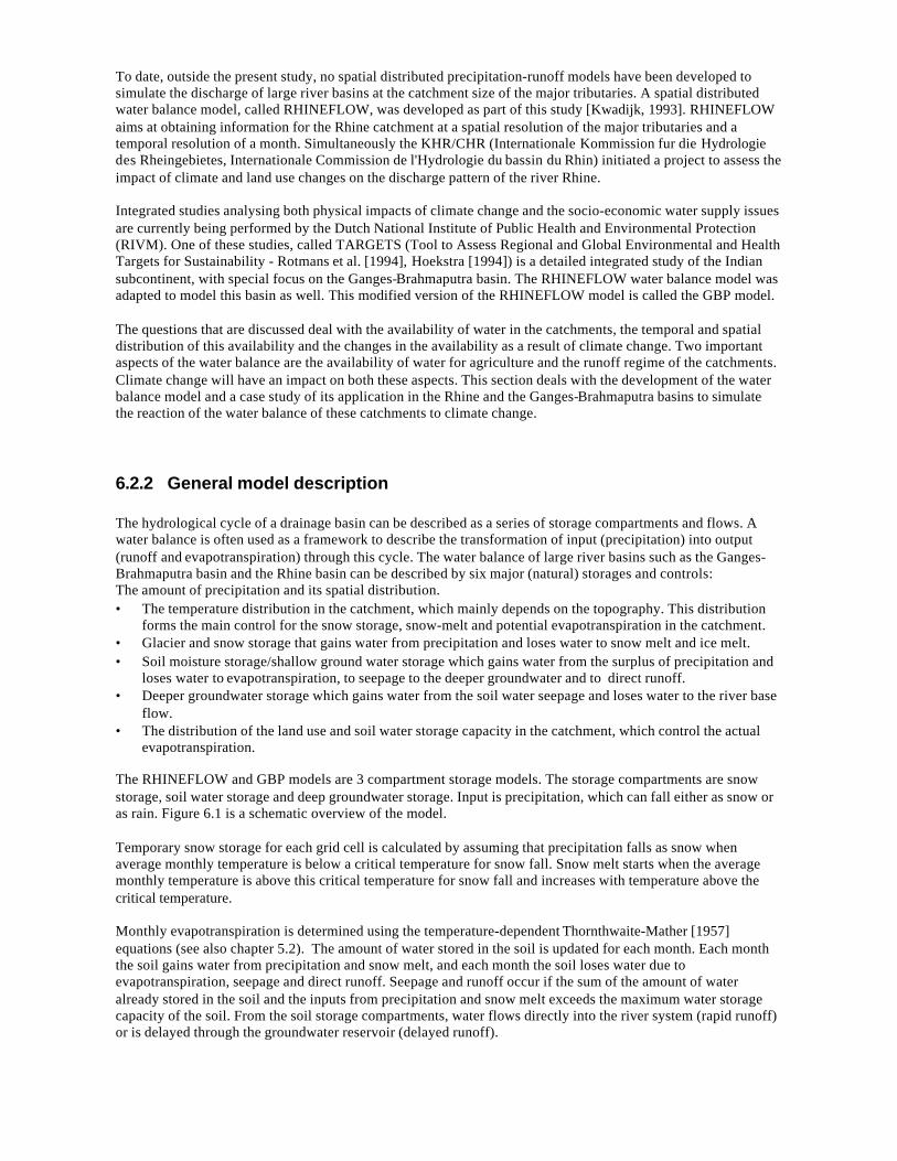
To date, outside the present study, no spatial distributed precipitation-runoff models have been developed tosimulate the discharge of large river basins at the catchment size of the major tributaries. A spatial distributedwater balance model, called RHINEFLOW, was developed as part of this study [Kwadijk, 1993]. RHINEFLOWaims at obtaining information for the Rhine catchment at a spatial resolution of the major tributaries and atemporal resolution of a month. Simultaneously the KHR/CHR (Internationale Kommission fur die Hydrologiedes Rheingebietes, Internationale Commission de l'Hydrologie du bassin du Rhin) initiated a project to assess theimpact of climate and land use changes on the discharge pattern of the river Rhine.

Integrated studies analysing both physical impacts of climate change and the socio-economic water supply issuesare currently being performed by the Dutch National Institute of Public Health and Environmental Protection(RIVM). One of these studies, called TARGETS (Tool to Assess Regional and Global Environmental and HealthTargets for Sustainability - Rotmans et al. [1994], Hoekstra [1994]) is a detailed integrated study of the Indiansubcontinent, with special focus on the Ganges-Brahmaputra basin. The RHINEFLOW water balance model wasadapted to model this basin as well. This modified version of the RHINEFLOW model is called the GBP model.

The questions that are discussed deal with the availability of water in the catchments, the temporal and spatialdistribution of this availability and the changes in the availability as a result of climate change. Two importantaspects of the water balance are the availability of water for agriculture and the runoff regime of the catchments.Climate change will have an impact on both these aspects. This section deals with the development of the waterbalance model and a case study of its application in the Rhine and the Ganges-Brahmaputra basins to simulatethe reaction of the water balance of these catchments to climate change.

6.2.2 General model description

The hydrological cycle of a drainage basin can be described as a series of storage compartments and flows. Awater balance is often used as a framework to describe the transformation of input (precipitation) into output(runoff and evapotranspiration) through this cycle. The water balance of large river basins such as the Ganges-Brahmaputra basin and the Rhine basin can be described by six major (natural) storages and controls:The amount of precipitation and its spatial distribution.• The temperature distribution in the catchment, which mainly depends on the topography. This distribution

forms the main control for the snow storage, snow-melt and potential evapotranspiration in the catchment.• Glacier and snow storage that gains water from precipitation and loses water to snow melt and ice melt.• Soil moisture storage/shallow ground water storage which gains water from the surplus of precipitation and

loses water to evapotranspiration, to seepage to the deeper groundwater and to direct runoff.• Deeper groundwater storage which gains water from the soil water seepage and loses water to the river base

flow.• The distribution of the land use and soil water storage capacity in the catchment, which control the actual

evapotranspiration.

The RHINEFLOW and GBP models are 3 compartment storage models. The storage compartments are snowstorage, soil water storage and deep groundwater storage. Input is precipitation, which can fall either as snow oras rain. Figure 6.1 is a schematic overview of the model.

Temporary snow storage for each grid cell is calculated by assuming that precipitation falls as snow whenaverage monthly temperature is below a critical temperature for snow fall. Snow melt starts when the averagemonthly temperature is above this critical temperature for snow fall and increases with temperature above thecritical temperature.

Monthly evapotranspiration is determined using the temperature-dependent Thornthwaite-Mather [1957]equations (see also chapter 5.2). The amount of water stored in the soil is updated for each month. Each monththe soil gains water from precipitation and snow melt, and each month the soil loses water due toevapotranspiration, seepage and direct runoff. Seepage and runoff occur if the sum of the amount of wateralready stored in the soil and the inputs from precipitation and snow melt exceeds the maximum water storagecapacity of the soil. From the soil storage compartments, water flows directly into the river system (rapid runoff)or is delayed through the groundwater reservoir (delayed runoff).

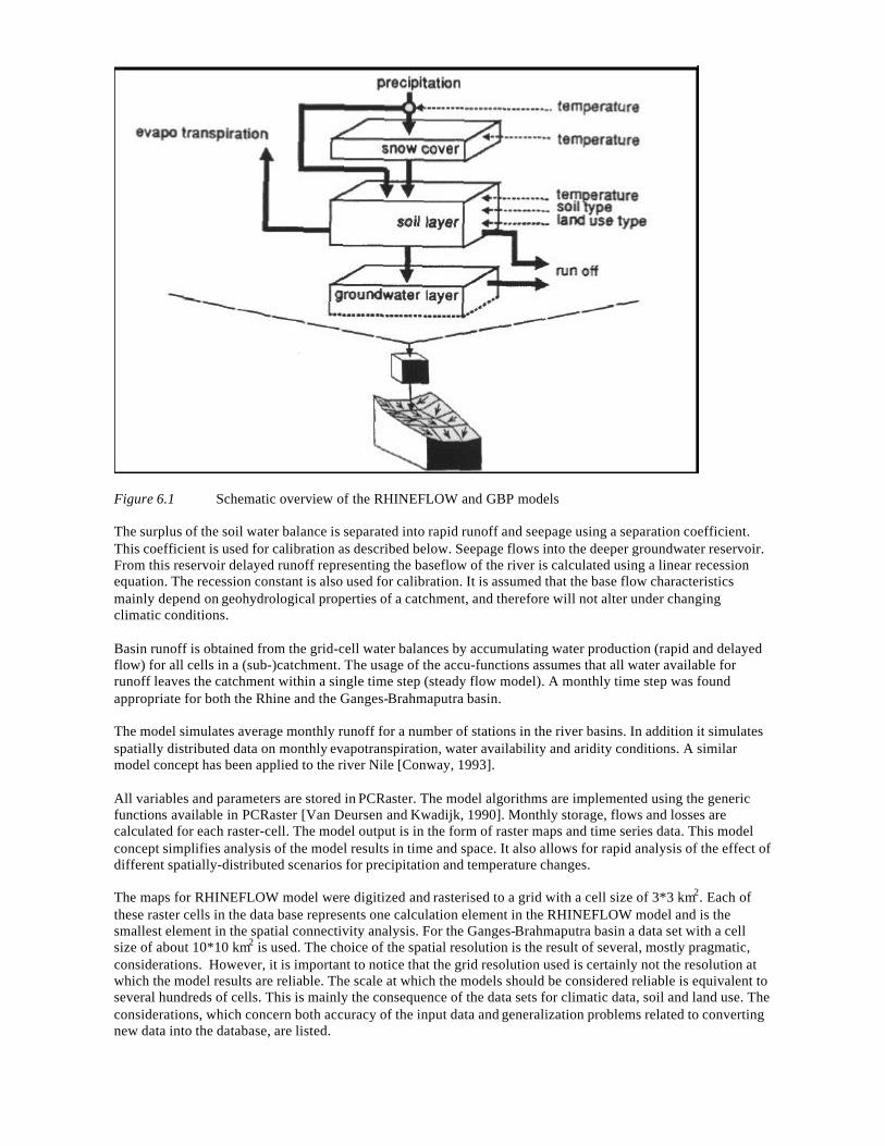
Figure 6.1 Schematic overview of the RHINEFLOW and GBP models

The surplus of the soil water balance is separated into rapid runoff and seepage using a separation coefficient.This coefficient is used for calibration as described below. Seepage flows into the deeper groundwater reservoir.From this reservoir delayed runoff representing the baseflow of the river is calculated using a linear recessionequation. The recession constant is also used for calibration. It is assumed that the base flow characteristicsmainly depend on geohydrological properties of a catchment, and therefore will not alter under changingclimatic conditions.

Basin runoff is obtained from the grid-cell water balances by accumulating water production (rapid and delayedflow) for all cells in a (sub-)catchment. The usage of the accu-functions assumes that all water available forrunoff leaves the catchment within a single time step (steady flow model). A monthly time step was foundappropriate for both the Rhine and the Ganges-Brahmaputra basin.

The model simulates average monthly runoff for a number of stations in the river basins. In addition it simulatesspatially distributed data on monthly evapotranspiration, water availability and aridity conditions. A similarmodel concept has been applied to the river Nile [Conway, 1993].

All variables and parameters are stored in PCRaster. The model algorithms are implemented using the genericfunctions available in PCRaster [Van Deursen and Kwadijk, 1990]. Monthly storage, flows and losses arecalculated for each raster-cell. The model output is in the form of raster maps and time series data. This modelconcept simplifies analysis of the model results in time and space. It also allows for rapid analysis of the effect ofdifferent spatially-distributed scenarios for precipitation and temperature changes.

The maps for RHINEFLOW model were digitized and rasterised to a grid with a cell size of 3*3 km2. Each ofthese raster cells in the data base represents one calculation element in the RHINEFLOW model and is thesmallest element in the spatial connectivity analysis. For the Ganges-Brahmaputra basin a data set with a cellsize of about 10*10 km2 is used. The choice of the spatial resolution is the result of several, mostly pragmatic,considerations. However, it is important to notice that the grid resolution used is certainly not the resolution atwhich the model results are reliable. The scale at which the models should be considered reliable is equivalent toseveral hundreds of cells. This is mainly the consequence of the data sets for climatic data, soil and land use. Theconsiderations, which concern both accuracy of the input data and generalization problems related to convertingnew data into the database, are listed.

• Topographical data was derived from maps with scales of 1:1,500,000 (Rhine catchment), 1:2,000,000 and1:6,000,000 (Ganges-Brahmaputra catchment). On the maps of 1:1,500,000 a length of 2 mm represents adistance of 3 km and this length is assumed to be the maximum resolution of the spatial information of thesemaps.

• This resolution permits the accurate location of gauging stations along the rivers and the main tributaries.• The model is designed for use on a personal computer. At time of the development of the model (1990),

using this resolution a model run for 25 years took six hours on a PC (PC with 80386 processor and 8MbRAM).

• The model is designed for the assessment of the impact of climate change. The changes in temperature andprecipitation resulting from GCM's (Global Circulation Models) have been interpolated onto a grid of 0.5degree latitude and 1.0 degree longitude using present day climate information (Climate Research GroupUniversity of East Anglia and Environmental Resources Limited, unpublished data). The used 3*3 km2 and10*10 km2 grid are of higher resolution, and allow conversion of the scenario changes into the databasewithout generalization problems.

The use of this grid size has some important limitations, namely:• Calculations of slope gradient, exposition and local drain direction from a DEM having a 3*3 km2 (or 10*10

km2) resolution do have a physical meaning, but it is not the usual one expected. These slopes show thedirections of the change of the underlying elevation surface, and can be used to create the topological linksin the local drain direction maps. The slopes cannot be expected to represent local slopes that can bemeasured in the field. Therefore, an accurate estimate for the process of overland flow is not possible withthis modelling concept. Hence, flows like Hortonian overland flow, interflow and saturated overland floware not incorporated into the model. The model has been developed to analyse the discharge of major riversand their tributaries on a monthly time basis. Using this time basis and catchment scale, estimates of theindividual contributions of different flows (saturated and Hortonian overland flow, interflow andgroundwater flow) to the streamflow are difficult to make.

• Detailed physically based models to determine snow melt and snow accumulation cannot be used sincethese models strongly depend on local slope exposition.

• Since the river channels in the river basins are in general narrower than the grid size used, the drainageanalysis does not make any statements about the nature of the channels (braided, meandering oranastomosing).

• The model concepts used here do not allow for any divergent stream patterns in the river network. However,in the concept of a hydrological catchment, which is used here, it is assumed that all excess water availablein the catchment will eventually flow to the outlet. This widely used concept does not allow for divergentstreams either.

Calibration of the model

Two criteria are used to calibrate the model. The first criterion is that the simulated annual runoff shouldcorrespond with the measured annual runoff, assuming a stable model. This assumption requires a zero change inaverage annual storage in glaciers, soil water and ground water. The second criterion is that the timing andmagnitude of peak and low flows (on a monthly time basis) should be well represented.

A measure to reflect the goodness of fit of the calculated hydrograph against the observed one is the coefficientof efficiency [Nash and Sutcliff, 1970]. A value of 1.0 for the coefficient of efficiency represents a perfect fit,values less than 0.0 mean that the average is a better representation than the model result. The coefficient ofefficiency seems to reflect the general conclusions of model performance according to visual inspection fairlywell [Bergström, 1976].

An optimal calibration and validation scheme includes a separation between dry and wet periods for calibrationand validation purposes [Klemes, 1986b], which requires a long record of observations. One of the periods(either the dry period or the wet period) is used for calibrating the model, the other is used for validationpurposes.

To meet the first criterion, the model is run until the groundwater storage change and snow storage change overthe year is zero. The snow module was calibrated so that snow cover duration was 12 months per year in cellsidentified as glaciers on land use maps. The accumulation and decay of the snow cover in these cells was kept inbalance over the years. In all other cells the snow cover disappeared completely for at least one month per year.

The critical temperature for snow fall was kept at 0o Celsius.

The procedure followed to meet the second criterion is to run the model, using the above snow moduleparameters, for 12 months to represent an average year. The separation coefficient and the recession coefficientare calibrated in simultaneously so that the model efficiency is maximised for this average year.

6.2.3 Modelling the effects of climate change on river discharge in the Rhinebasin

Hydrological setting of the Rhine basin

In Western Europe the river Rhine is the most important river. Its basin of approximately 250,000 km2 stretchesfrom the Alps to the North Sea. Two thirds of the basin is situated in Germany. The Alpine countries, of whichSwitzer-land is the most important, form 20% of the area. The river has the world's highest traffic density forinland waterways. Besides this navigation its economic importance is great because it is the major water supplyfor industrial, domestic and agricultural purposes. In addition, in the downstream region (The Netherlands) largeamounts of Rhine water are used to prevent salt intrusion from the groundwater in the polders [CHR/KHR,1976]. Possible future changes in discharge and river behaviour as a result of a climatic change may have largeimpact on the above mentioned water use.

Figure 6.2 a Hydrograph Rheinfeldenb Hydrograph Rees

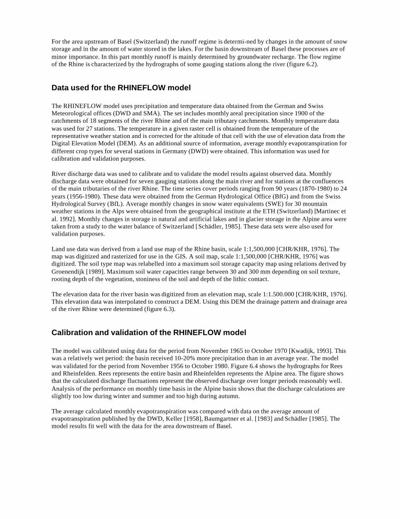
For the area upstream of Basel (Switzerland) the runoff regime is determi-ned by changes in the amount of snowstorage and in the amount of water stored in the lakes. For the basin downstream of Basel these processes are ofminor importance. In this part monthly runoff is mainly determined by groundwater recharge. The flow regimeof the Rhine is characterized by the hydrographs of some gauging stations along the river (figure 6.2).

Data used for the RHINEFLOW model

The RHINEFLOW model uses precipitation and temperature data obtained from the German and SwissMeteorological offices (DWD and SMA). The set includes monthly areal precipitation since 1900 of thecatchments of 18 segments of the river Rhine and of the main tributary catchments. Monthly temperature datawas used for 27 stations. The temperature in a given raster cell is obtained from the temperature of therepresentative weather station and is corrected for the altitude of that cell with the use of elevation data from theDigital Elevation Model (DEM). As an additional source of information, average monthly evapotranspiration fordifferent crop types for several stations in Germany (DWD) were obtained. This information was used forcalibration and validation purposes.

River discharge data was used to calibrate and to validate the model results against observed data. Monthlydischarge data were obtained for seven gauging stations along the main river and for stations at the confluencesof the main tributaries of the river Rhine. The time series cover periods ranging from 90 years (1870-1980) to 24years (1956-1980). These data were obtained from the German Hydrological Office (BfG) and from the SwissHydrological Survey (BfL). Average monthly changes in snow water equivalents (SWE) for 30 mountainweather stations in the Alps were obtained from the geographical institute at the ETH (Switzerland) [Martinec etal. 1992]. Monthly changes in storage in natural and artificial lakes and in glacier storage in the Alpine area weretaken from a study to the water balance of Switzerland [Schädler, 1985]. These data sets were also used forvalidation purposes.

Land use data was derived from a land use map of the Rhine basin, scale 1:1,500,000 [CHR/KHR, 1976]. Themap was digitized and rasterized for use in the GIS. A soil map, scale 1:1,500,000 [CHR/KHR, 1976] wasdigitized. The soil type map was relabelled into a maximum soil storage capacity map using relations derived byGroenendijk [1989]. Maximum soil water capacities range between 30 and 300 mm depending on soil texture,rooting depth of the vegetation, stoniness of the soil and depth of the lithic contact.

The elevation data for the river basin was digitized from an elevation map, scale 1:1.500.000 [CHR/KHR, 1976].This elevation data was interpolated to construct a DEM. Using this DEM the drainage pattern and drainage areaof the river Rhine were determined (figure 6.3).

Calibration and validation of the RHINEFLOW model

The model was calibrated using data for the period from November 1965 to October 1970 [Kwadijk, 1993]. Thiswas a relatively wet period: the basin received 10-20% more precipitation than in an average year. The modelwas validated for the period from November 1956 to October 1980. Figure 6.4 shows the hydrographs for Reesand Rheinfelden. Rees represents the entire basin and Rheinfelden represents the Alpine area. The figure showsthat the calculated discharge fluctuations represent the observed discharge over longer periods reasonably well.Analysis of the performance on monthly time basis in the Alpine basin shows that the discharge calculations areslightly too low during winter and summer and too high during autumn.

The average calculated monthly evapotranspiration was compared with data on the average amount ofevapotranspiration published by the DWD, Keller [1958], Baumgartner et al. [1983] and Schädler [1985]. Themodel results fit well with the data for the area downstream of Basel.

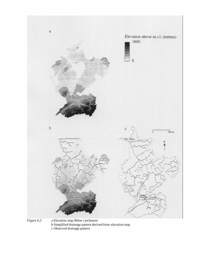
Figure 6.3 a Elavation map Rhine catchmentb Simplified drainage pattern derived from elavation mapc Observed drainage pattern

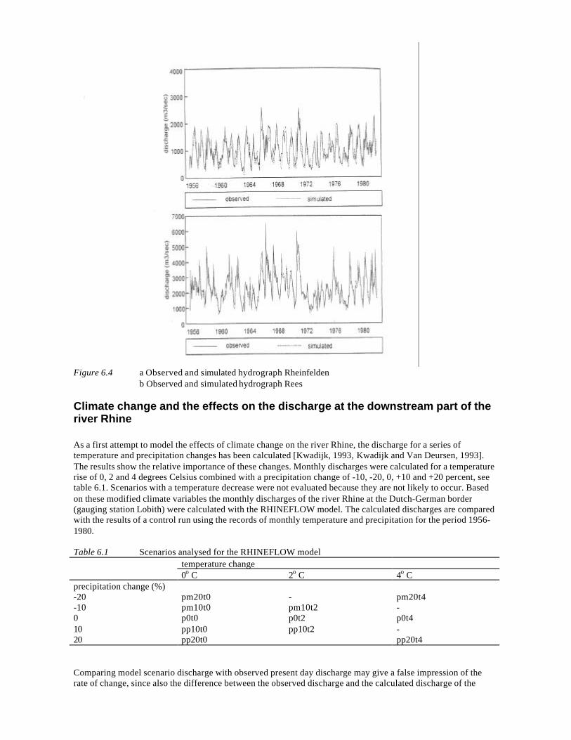
Figure 6.4 a Observed and simulated hydrograph Rheinfeldenb Observed and simulated hydrograph Rees

Climate change and the effects on the discharge at the downstream part of theriver Rhine

As a first attempt to model the effects of climate change on the river Rhine, the discharge for a series oftemperature and precipitation changes has been calculated [Kwadijk, 1993, Kwadijk and Van Deursen, 1993].The results show the relative importance of these changes. Monthly discharges were calculated for a temperaturerise of 0, 2 and 4 degrees Celsius combined with a precipitation change of -10, -20, 0, +10 and +20 percent, seetable 6.1. Scenarios with a temperature decrease were not evaluated because they are not likely to occur. Basedon these modified climate variables the monthly discharges of the river Rhine at the Dutch-German border(gauging station Lobith) were calculated with the RHINEFLOW model. The calculated discharges are comparedwith the results of a control run using the records of monthly temperature and precipitation for the period 1956-1980.

Table 6.1 Scenarios analysed for the RHINEFLOW modeltemperature change0o C 2o C 4o C

precipitation change (%)-20 pm20t0 - pm20t4-10 pm10t0 pm10t2 -0 p0t0 p0t2 p0t410 pp10t0 pp10t2 -20 pp20t0 pp20t4

Comparing model scenario discharge with observed present day discharge may give a false impression of therate of change, since also the difference between the observed discharge and the calculated discharge of the

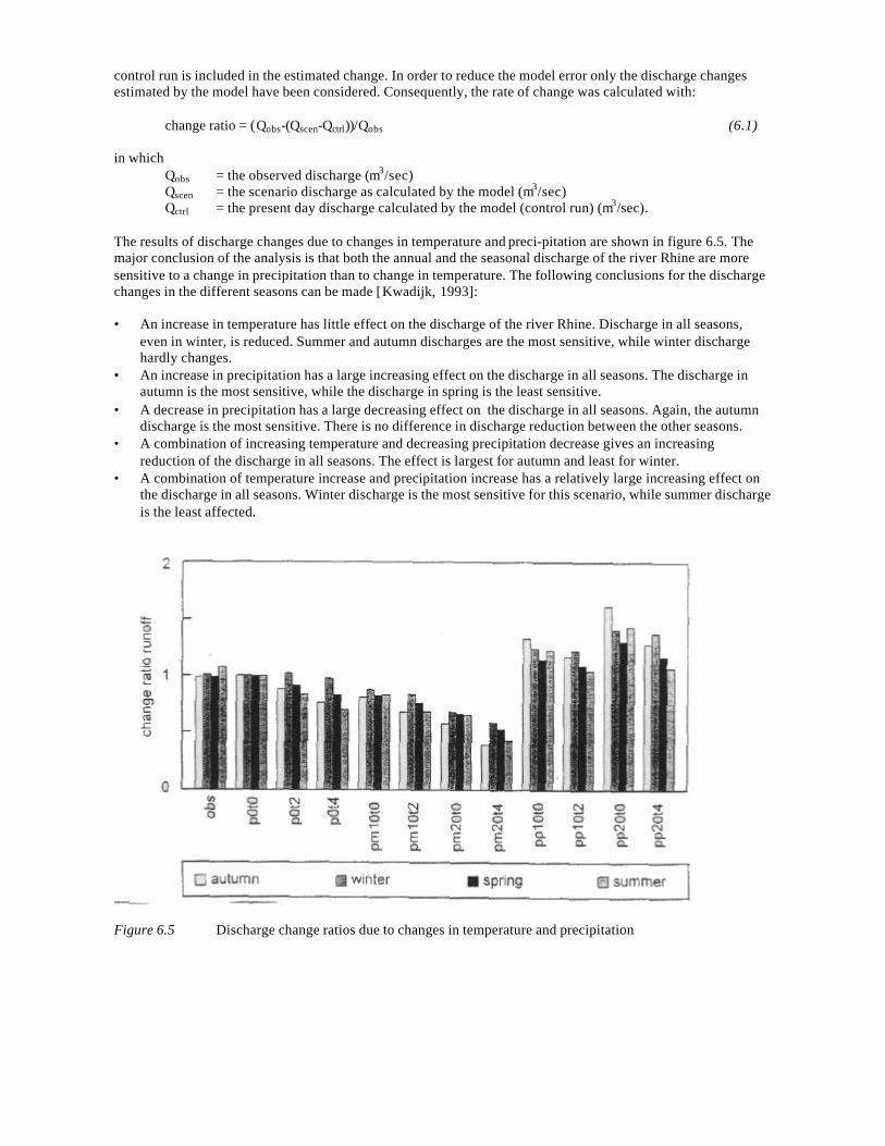
control run is included in the estimated change. In order to reduce the model error only the discharge changesestimated by the model have been considered. Consequently, the rate of change was calculated with:

change ratio = (Qobs-(Qscen-Qctrl))/Qobs (6.1)

in whichQobs = the observed discharge (m3/sec)Qscen = the scenario discharge as calculated by the model (m3/sec)Qctrl = the present day discharge calculated by the model (control run) (m3/sec).

The results of discharge changes due to changes in temperature and preci-pitation are shown in figure 6.5. Themajor conclusion of the analysis is that both the annual and the seasonal discharge of the river Rhine are moresensitive to a change in precipitation than to change in temperature. The following conclusions for the dischargechanges in the different seasons can be made [Kwadijk, 1993]:

• An increase in temperature has little effect on the discharge of the river Rhine. Discharge in all seasons,even in winter, is reduced. Summer and autumn discharges are the most sensitive, while winter dischargehardly changes.

• An increase in precipitation has a large increasing effect on the discharge in all seasons. The discharge inautumn is the most sensitive, while the discharge in spring is the least sensitive.

• A decrease in precipitation has a large decreasing effect on the discharge in all seasons. Again, the autumndischarge is the most sensitive. There is no difference in discharge reduction between the other seasons.

• A combination of increasing temperature and decreasing precipitation decrease gives an increasingreduction of the discharge in all seasons. The effect is largest for autumn and least for winter.

• A combination of temperature increase and precipitation increase has a relatively large increasing effect onthe discharge in all seasons. Winter discharge is the most sensitive for this scenario, while summer dischargeis the least affected.

Figure 6.5 Discharge change ratios due to changes in temperature and precipitation

6.2.4 Modelling the effects of climate change on river discharge in the Ganges-Brahmaputra basin

Hydrological setting of the Ganges-Brahmaputra basin

The Ganges flows from the Nepalese Himalayas through its Ganges plain in India and confluences with theBrahmaputra in Bangladesh. The catchment of the Ganges covers an area estimated as between 975 and 1,073thousand square kilometres. The basin size of the Brahmaputra is estimated as between 530 and 938 thousandsquare kilometres [Gleick, 1993]. Average annual runoff of the Ganges is in the range of 15,000 m3/sec and forthe Brahmaputra this amounts 20,000 m3/sec. Both river regimes are almost completely determined by thesummer monsoon. During the monsoon the runoff in the downstream part of the Brahmaputra increases to45,000 m3/sec. During the dry period the discharge is reduced to 3,700 m3/sec. The River Ganges produces37,000 m3/sec during the monsoon and 1,700 m3/sec during the dry period.

The river Ganges flows through the low land of India where much of its water is used for irrigation. TheBrahmaputra flows from the dry high altitude plain in Tibet to Bangladesh. Upstream of Bangladesh only littleof its water is used for agricultural purposes.

The RHINEFLOW model described above was slightly modified for use in the Ganges-Brahmaputra basin. Thenew model is called the GBP model, and the modifications from the RHINEFLOW model are:• creating a new spatial database with input maps for the model;• creating a new climate database and allow for a modified definition of climate change scenarios;• determine new values for calibrated parameters and variables; and• include analysis of aridity and length of growing season.

The GBP model incorporates the aridity index AI as described in chapter 5. To include these modificationsrequired the change of approximately 10 lines of PCRaster code.

Climate data for the Ganges-Brahmaputra model

The model for the Ganges-Brahmaputra uses precipitation and temperature data from the IIASA climatedatabase. This database contains long-term monthly average climate data on a grid of 0.5*0.5 degree longitude-latitude from the reference period 1960-1980. In addition to this data the model uses time series of climate datafrom weather stations in the basin from the World Climate Disk (WCD-database) [CRU, 1992]. We used theIIASA grid data to calibrate the model. The model was validated using long-term time series for temperature andprecipitation. The time series were derived by combining the average monthly data of the IIASA database withthe month to month deviation for the period considered, using:

Tx,y,t = Tx,y,t avg + dTx,y,t (oC)

and

Px,y,t = Px,y,t avg + Px,y,t avg*dPx,y,t /100 (mm)

in whichTt avg = long-term average monthly temperature (oC) (IIASA database);dTt = temperature deviation from reference period temperature in month t at the representative

station (oC) (CRU-WCD database);Pt avg = long-term average monthly precipitation (mm) (IIASA database);dPt = precipitation deviation (percentage) from the reference period precipitation in month t at the

representative station (CRU-WCD database).

Although this is a different method of deriving input data than used in the RHINEFLOW model, implementationrequired changing two lines of PCRaster code only.

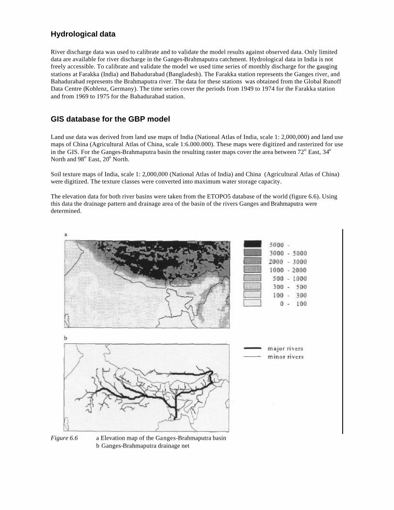
Hydrological data

River discharge data was used to calibrate and to validate the model results against observed data. Only limiteddata are available for river discharge in the Ganges-Brahmaputra catchment. Hydrological data in India is notfreely accessible. To calibrate and validate the model we used time series of monthly discharge for the gaugingstations at Farakka (India) and Bahadurabad (Bangladesh). The Farakka station represents the Ganges river, andBahadurabad represents the Brahmaputra river. The data for these stations was obtained from the Global RunoffData Centre (Koblenz, Germany). The time series cover the periods from 1949 to 1974 for the Farakka stationand from 1969 to 1975 for the Bahadurabad station.

GIS database for the GBP model

Land use data was derived from land use maps of India (National Atlas of India, scale 1: 2,000,000) and land usemaps of China (Agricultural Atlas of China, scale 1:6.000.000). These maps were digitized and rasterized for usein the GIS. For the Ganges-Brahmaputra basin the resulting raster maps cover the area between 72o East, 34o

North and 98o East, 20o North.

Soil texture maps of India, scale 1: 2,000,000 (National Atlas of India) and China (Agricultural Atlas of China)were digitized. The texture classes were converted into maximum water storage capacity.

The elevation data for both river basins were taken from the ETOPO5 database of the world (figure 6.6). Usingthis data the drainage pattern and drainage area of the basin of the rivers Ganges and Brahmaputra weredetermined.

Figure 6.6 a Elevation map of the Ganges-Brahmaputra basinb Ganges-Brahmaputra drainage net

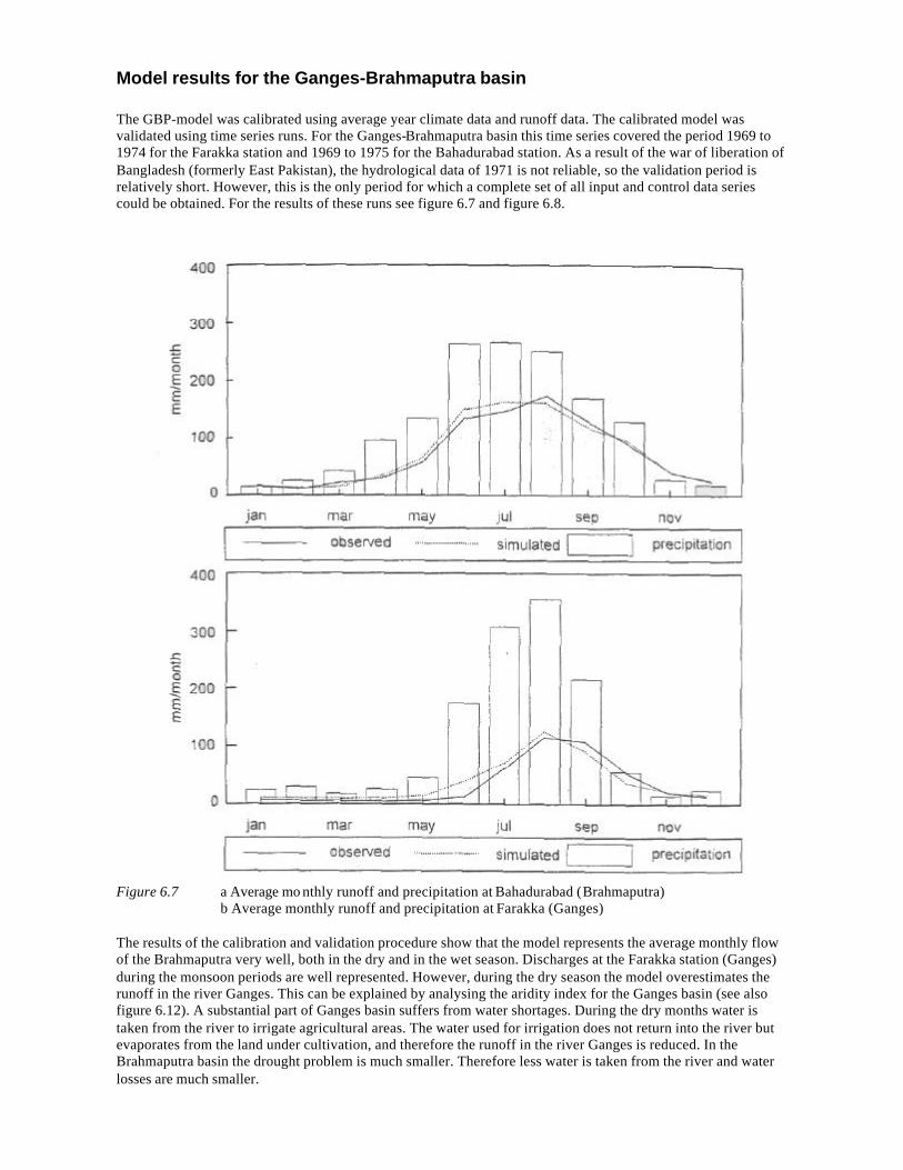
Model results for the Ganges-Brahmaputra basin

The GBP-model was calibrated using average year climate data and runoff data. The calibrated model wasvalidated using time series runs. For the Ganges-Brahmaputra basin this time series covered the period 1969 to1974 for the Farakka station and 1969 to 1975 for the Bahadurabad station. As a result of the war of liberation ofBangladesh (formerly East Pakistan), the hydrological data of 1971 is not reliable, so the validation period isrelatively short. However, this is the only period for which a complete set of all input and control data seriescould be obtained. For the results of these runs see figure 6.7 and figure 6.8.

Figure 6.7 a Average mo nthly runoff and precipitation at Bahadurabad (Brahmaputra)b Average monthly runoff and precipitation at Farakka (Ganges)

The results of the calibration and validation procedure show that the model represents the average monthly flowof the Brahmaputra very well, both in the dry and in the wet season. Discharges at the Farakka station (Ganges)during the monsoon periods are well represented. However, during the dry season the model overestimates therunoff in the river Ganges. This can be explained by analysing the aridity index for the Ganges basin (see alsofigure 6.12). A substantial part of Ganges basin suffers from water shortages. During the dry months water istaken from the river to irrigate agricultural areas. The water used for irrigation does not return into the river butevaporates from the land under cultivation, and therefore the runoff in the river Ganges is reduced. In theBrahmaputra basin the drought problem is much smaller. Therefore less water is taken from the river and waterlosses are much smaller.

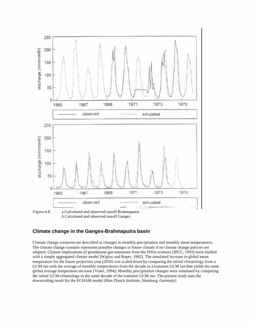
Figure 6.8 a Calculated and observed runoff Brahmaputrab Calculated and observed runoff Ganges

Climate change in the Ganges-Brahmaputra basin

Climate change scenarios are described as changes in monthly precipitation and monthly mean temperatures.The climate change scenario represents possible changes in future climate if no climate change policies areadapted. Climate implications of greenhouse gas emissions from the IS92a scenario [IPCC, 1992] were studiedwith a simple aggregated climate model [Wigley and Raper, 1992]. The simulated increase in global meantemperature for the future projection year (2050) was scaled down by comparing the initial climatology from aGCM run with the average of monthly temperatures from the decade in a transient GCM run that yields the sameglobal average temperature increase [Viner, 1994]. Monthly precipitation changes were simulated by comparingthe initial GCM climatology to the same decade of the transient GCM run. The present study uses thedownscaling result for the ECHAM model (Max Planck Institute, Hamburg, Germany).

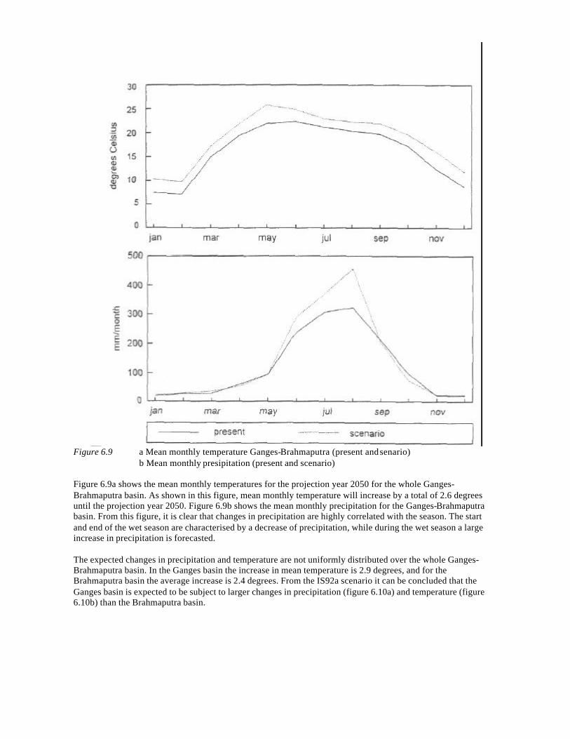
Figure 6.9 a Mean monthly temperature Ganges-Brahmaputra (present and senario)b Mean monthly presipitation (present and scenario)

Figure 6.9a shows the mean monthly temperatures for the projection year 2050 for the whole Ganges-Brahmaputra basin. As shown in this figure, mean monthly temperature will increase by a total of 2.6 degreesuntil the projection year 2050. Figure 6.9b shows the mean monthly precipitation for the Ganges-Brahmaputrabasin. From this figure, it is clear that changes in precipitation are highly correlated with the season. The startand end of the wet season are characterised by a decrease of precipitation, while during the wet season a largeincrease in precipitation is forecasted.

The expected changes in precipitation and temperature are not uniformly distributed over the whole Ganges-Brahmaputra basin. In the Ganges basin the increase in mean temperature is 2.9 degrees, and for theBrahmaputra basin the average increase is 2.4 degrees. From the IS92a scenario it can be concluded that theGanges basin is expected to be subject to larger changes in precipitation (figure 6.10a) and temperature (figure6.10b) than the Brahmaputra basin.

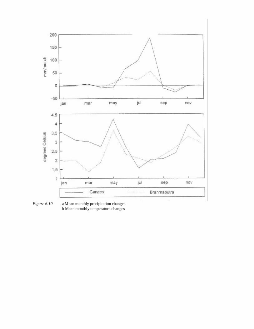
Figure 6.10 a Mean monthly precipitation changesb Mean monthly temperature changes

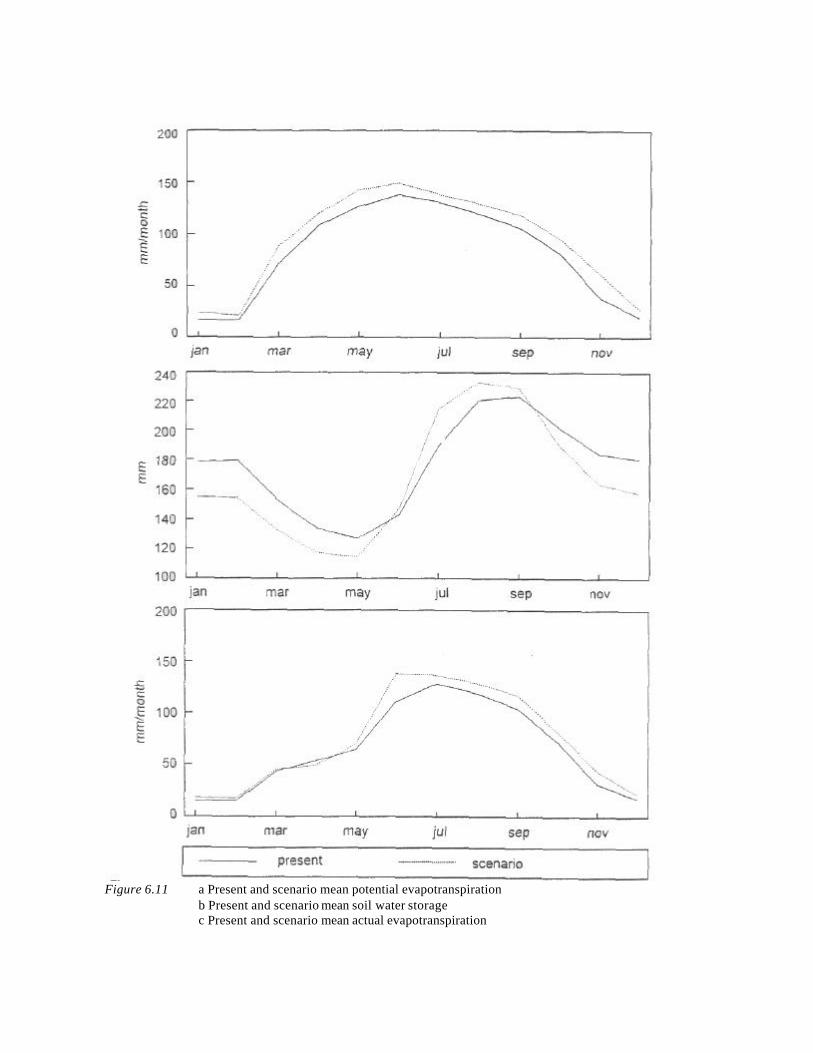
Figure 6.11 a Present and scenario mean potential evapotranspirationb Present and scenario mean soil water storagec Present and scenario mean actual evapotranspiration

Changes in soil water storage, aridity index and evapotranspiration due toclimate change

As monthly evapotranspiration is closely correlated with the monthly mean temperatures, the changes intemperature will immediately affect the potential evapotranspiration. The results of the model for simulating themean monthly evapotranspiration for the projection year 2050 are represented in figure 6.11. An averageincrease of potential evapotranspiration of 11.8 mm/month can be expected for the projection year 2050 fromanalysing the results of the scenario runs.

The surplus of precipitation will ensure that the soils will be at maximum water holding capacity at the end ofthe wet season. Due to increased evapotranspiration, the amount of water stored in the soil at the end of the dryseason will be decreased (figure 6.11b). As a result, a larger soil water deficiency at the end of the dry seasonwill occur compared to the present situation. This deficiency in soil water means that the soil will not containenough water to fulfil the demands of potential evapotranspiration completely. As a result of this waterdeficiency, the increase in monthly actual evapotranspiration is limited to about 7.6 mm/month as compared toan increase of potential evapotranspiration of 11.8 mm/month.

As explained in chapter 5, the aridity index AI is an important indicator for water shortage and water demand.For the projection year 2050 the aridity index is given in figure 6.12 and table 6.1. From this figure, it can beconcluded that the aridity situation will deteriorate as a result of climate change.

Table 6.2 Average aridity index for the total catchment and the subcatchments of Ganges andBrahmaputra

Total basin Ganges1) Brahmaputra1)

present situation 0.12 0.20 0.01projection year 2050 0.15 0.24 0.021) Ganges Basin is the area upstream of gauging station at Farakka

Brahmaputra basin is the area upstream of gauging station at Bahadurabad

The aridity conditions in the Ganges basin are very different from the aridity conditions in the Brahmaputrabasin. Analysing the maps of distribution of the aridity index yields the conclusion that the problem of aridity ismuch more pronounced in the Ganges basin than in the Brahmaputra basin. This may be explained by the factthat a large part of the Brahmaputra basin is in areas with high precipitation or at high elevation in theHimalayas, where temperatures are too low to cause a large potential evapotranspiration. The aridity indices forthe different parts of the catchment are given in table 6.2.

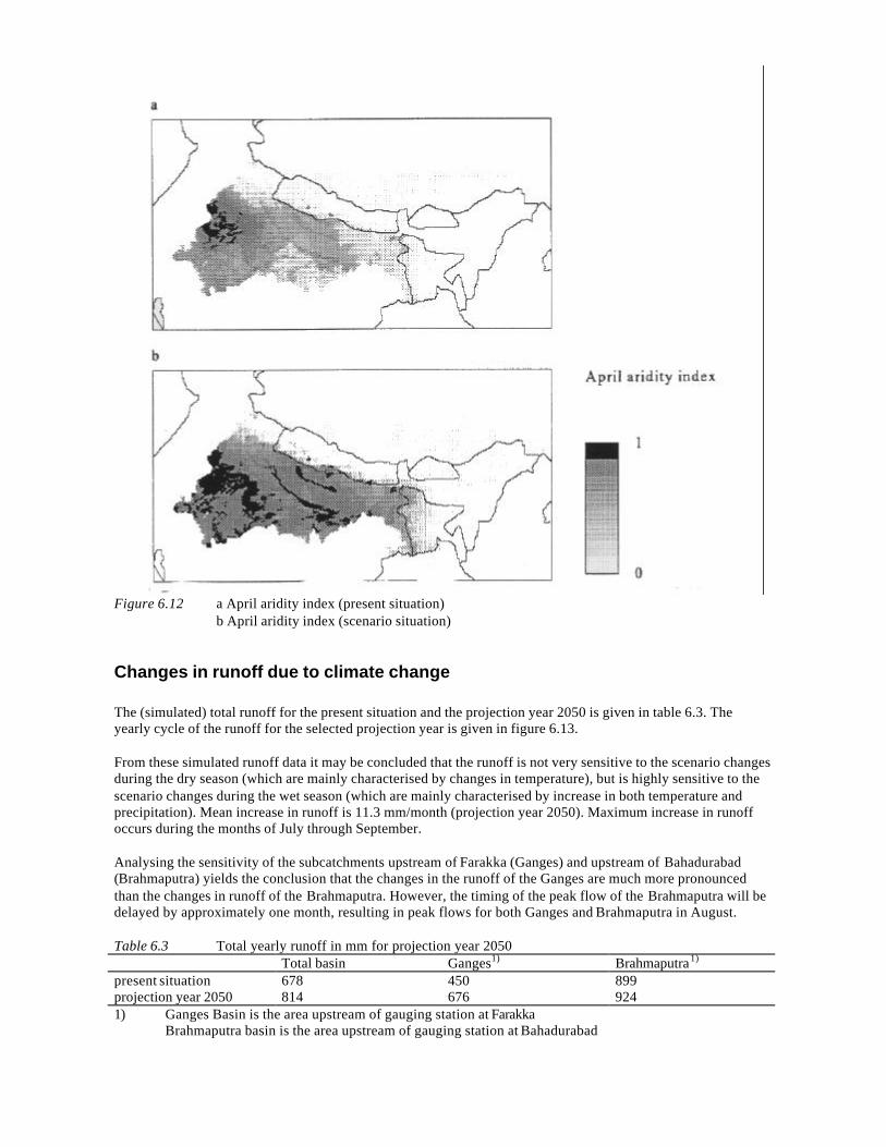
Figure 6.12 a April aridity index (present situation)b April aridity index (scenario situation)

Changes in runoff due to climate change

The (simulated) total runoff for the present situation and the projection year 2050 is given in table 6.3. Theyearly cycle of the runoff for the selected projection year is given in figure 6.13.

From these simulated runoff data it may be concluded that the runoff is not very sensitive to the scenario changesduring the dry season (which are mainly characterised by changes in temperature), but is highly sensitive to thescenario changes during the wet season (which are mainly characterised by increase in both temperature andprecipitation). Mean increase in runoff is 11.3 mm/month (projection year 2050). Maximum increase in runoffoccurs during the months of July through September.

Analysing the sensitivity of the subcatchments upstream of Farakka (Ganges) and upstream of Bahadurabad(Brahmaputra) yields the conclusion that the changes in the runoff of the Ganges are much more pronouncedthan the changes in runoff of the Brahmaputra. However, the timing of the peak flow of the Brahmaputra will bedelayed by approximately one month, resulting in peak flows for both Ganges and Brahmaputra in August.

Table 6.3 Total yearly runoff in mm for projection year 2050Total basin Ganges1) Brahmaputra1)

present situation 678 450 899projection year 2050 814 676 9241) Ganges Basin is the area upstream of gauging station at Farakka

Brahmaputra basin is the area upstream of gauging station at Bahadurabad

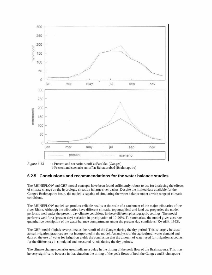
Figure 6.13 a Present and scenario runoff at Farakka (Ganges)b Present and scenario runoff at Bahadurabad (Brahmaputra)

6.2.5 Conclusions and recommendations for the water balance studies

The RHINEFLOW and GBP-model concepts have been found sufficiently robust to use for analysing the effectsof climate change on the hydrologic situation in large river basins. Despite the limited data available for theGanges-Brahmaputra basin, the model is capable of simulating the water balance under a wide range of climaticconditions.

The RHINEFLOW-model can produce reliable results at the scale of a catchment of the major tributaries of theriver Rhine. Although the tributaries have different climatic, topographical and land use properties the modelperforms well under the present-day climate conditions in these different physiographic settings. The modelperforms well for a (present day) variation in precipitation of 10-20%. To summarize, the model gives accuratequantitative description of the water balance compartments under the present-day conditions [Kwadijk, 1993].

The GBP-model slightly overestimates the runoff of the Ganges during the dry period. This is largely becauseactual irrigation practices are not incorporated in the model. An analysis of the agricultural water demand anddata on the use of water for irrigation yields the conclusion that the amount of water used for irrigation accountsfor the differences in simulated and measured runoff during the dry periods.

The climate change scenarios used indicate a delay in the timing of the peak flow of the Brahmaputra. This maybe very significant, because in that situation the timing of the peak flows of both the Ganges and Brahmaputra

will overlap. It can be concluded that both drought problems and flooding will increase. The increase in theseproblems is not uniformly distributed over the catchments. The model enables a detailed analysis of the positionand timing of periods of drought and flooding.

The RHINEFLOW model developed for the Rhine catchment proved to be robust enough to be used in theGanges-Brahmaputra basin. The modifications necessary for the different inputs and controls (physiographic,climate etcetera) were easily incorporated into the model. After calibrating the modified model, the results forthe Ganges-Brahmaputra basin proved to be reliable and useful. The model concept and the use of PCRaster forimplementing the model proved to be flexible and robust.

Another advantage of the models implemented in PCRaster is the capability to produce both maps of the spatialdistribution and timeseries of the temporal distribution of the results. Theoretically, this allows for the analysis ofthe soil water balance and drought conditions in different sub regions and for the analysis of runoff at a largenumber of points along the river network. Such an analysis is important for the analysis of the aridity situation ofsmaller regions, which is very much controlled by the position of the regions within the catchment. However,since only few discharge data sets were available, the reliability of the model results within these subcatchmentscannot be analysed. Therefore, the results produced by the model for these small catchments should be used withextreme care. Also, climate input is on a very coarse grid. Obviously, regional differences of climate and therelated water availability within these grids are obscured.

The water balance and runoff simulations of the Ganges-Brahmaputra basin with the climate change scenariosyield the conclusion that the two sub-basins (Ganges and Brahmaputra) have a very dissimilar reaction to climatechange. There are two major reasons for this. First the inputs taken from the IS92a scenario are substantiallydifferent for each of the sub catchments. Secondly the reaction of the catchments is different. During the wetperiod the Ganges basin is characterised by a substantial increase in runoff, while the reaction of theBrahmaputra is less pronounced. During the dry period the Ganges basin is much more subject to droughtconditions as is clear from the maps of the aridity index, a situation that will worsen as a result of climatechange. The Brahmaputra basin is much less influenced by drought situations, both in present day and scenariosituations. The increase of the aridity index for large parts of the Ganges basin will lead to a larger demand forwater for agricultural uses. The model approach allows for an extension to incorporate agricultural yieldresponse to changes in the water balance.

Acknowledgments

We thank Dr. Schädler of the Bundesamt für Landeshydrologie und Geologie in Switzerland, Dr. Braun, Prof.Lang and Dr. Rohrer from the ETH in Zürich, Switzerland and Dr.Wildenhahn of the Bundesamt fürGewasserkunde in Germany and the German Meteorological Survey for supplying the hydrological andmeteorolo-gical data for the RHINEFLOW model.

Large parts of the research on the changes in runoff regime for the Ganges-Brahmaputra basin were carried outfor the TARGETS project of the Dutch National Institute of Public Health and Environmental Protection(RIVM). Dr. Jan Rotmans, Arjen Hoekstra and Maarten Krol of the RIVM cooperated in the presented analysisof the changes in the runoff regime of the Ganges-Brahmaputra.

6.3 Analysis of heathland dynamics

6.3.1 Introduction

In the Netherlands, many heathlands formerly dominated by Calluna vulgaris (L.) Hull - so called dry inlandheathlands (Genisto-Callunetum) - have become dominated by grasses, especially by wavy hair grass(Deschampsia flexuosa (L.) Trin.). An evaluation of the extent of these changes in Dutch heathland using aerialphotographs shows that more than 30% of former heathland has been replaced by grassland [Van Kootwijk andVan der Voet, 1990].

It has been suggested that eutrophication of heathlands may be a significant factor in the replacement of heatherby grasses [De Smidt, 1979]. Field and laboratory experiments affirmed the importance of nutrients inheathlands [Aerts, 1989; Heil and Diemont, 1983]. However, during a heather beetle outbreak it was alsoobserved that Calluna vulgaris is more severely affected by heather beetles in the more heavily nitrogenfertilized vegetation [Heil and Diemont, 1983]. This observation suggests that the replacement of Callunavulgaris by grasses might not simply be due to the higher potential growth rate of the grasses under a higherlevel of nitrogen availability.

Until recently, it was assumed that sulphur dioxide is the environmentally most damaging air pollutant inWestern Europe. It has been suggested that the decline of many plant species in the Netherlands is caused byacidification of the environment [Van Dam et al., 1986]. Nowadays, however, the eutrophicating effects ofatmospheric nitrogen have become more evident. Eutrophication largely results from ammonia/ammoniumdeposition, originating from the liquid manure used in great quantities in the intensive farming system in theNetherlands [Van Breemen et al., 1982; Buijsman et al., 1987]. Heathland has a strong filtering effect onammonia/ammonium in which the canopy structure of the vegetation is an important factor [Heil et al., 1987;Bobbink et al., 1990].

It has been shown that increased nutrient availability results in a change in competition between Calluna andDeschampsia. Moreover, increased nutrient availability results in a higher nutrient content of the Calluna leaves[Aerts, 1989; Bobbink et al., 1990], and the results of rearing experiments show that increased nutrient content ofthe Calluna leaves results in better growth of the larvae of the heather beetle [Brunsting and Heil, 1985]. Fromthese results it is hypothesized that outbreaks of this beetle are stimulated by nitrogen enrichment, and becomemore severe and occurring more frequently. Outbreaks of the heather beetle occur under certain conditions offood availability and of microclimatic conditions [De Smidt, 1977]. There are no outbreaks in young Callunastands (< 5 years), because the percentage cover of the canopy of Calling must be more than approximately 50%.During an outbreak of this beetle plague Calluna plants die off almost completely over large areas [Berdowskiand Zeilinga, 1987]. The opening up of the dwarf shrub canopy enhances the growth of grasses due to anelimination of the competition from Calluna.

The deposition of atmospheric ammonia is not equally distributed but strongly depends on the number and sizeof local sources. Heil and Bobbink [1993] have developed a 1-dimensional simulation model, called 'Calluna', inwhich processes such as nitrogen cycling, heather beetle outbreaks and competition between plant species havebeen incorporated to describe the impact of atmospheric nitrogen deposition on the competition between Callunaand Deschampsia. The algorithms of this 1-dimensional model have been modified and used to build the spatialdistributed CalGIS model.

6.3.2 Calluna model

The model involves the growth of Calluna and Deschampsia. Growth is represented as the change in percentagecover of the plant species. Similar to the relation between biomass and diameter at breast height of trees a closerelation between biomass and percentage cover of plant species exists, and is often used to determine thestanding crop of the vegetation [Heil, 1984]. This relation is assumed linear for Calluna and Deschampsia andexpressed as:

B = C *β (6.2)

whereB = dry weight standing crop per square metre;C = percentage canopy cover of the species in a stand of vegetation per unit ground area; and β = conversion factor for the individual species.

The conversion factors of Calluna and Deschampsia are different because of differences in the structure of thecanopy. The Calluna canopy consists of woody parts, and brown and green leaves while the Deschampsiacanopy consists of green and yellow leaves.

The formulas for calculating the percentage cover for the two species are given by (see also section 5.7):

SCt+1 = SCt + rC * SCt * (K - SCt - αcd * SDt) /K (6.3)

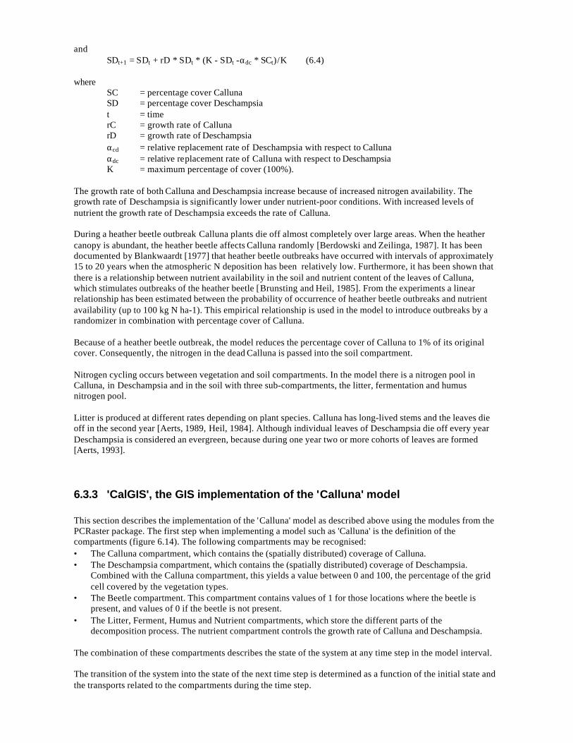
andSDt+1 = SDt + rD * SDt * (K - SDt -αdc * SCt)/K (6.4)

whereSC = percentage cover CallunaSD = percentage cover Deschampsiat = timerC = growth rate of CallunarD = growth rate of Deschampsiaαcd = relative replacement rate of Deschampsia with respect to Callunaαdc = relative replacement rate of Calluna with respect to DeschampsiaK = maximum percentage of cover (100%).

The growth rate of both Calluna and Deschampsia increase because of increased nitrogen availability. Thegrowth rate of Deschampsia is significantly lower under nutrient-poor conditions. With increased levels ofnutrient the growth rate of Deschampsia exceeds the rate of Calluna.

During a heather beetle outbreak Calluna plants die off almost completely over large areas. When the heathercanopy is abundant, the heather beetle affects Calluna randomly [Berdowski and Zeilinga, 1987]. It has beendocumented by Blankwaardt [1977] that heather beetle outbreaks have occurred with intervals of approximately15 to 20 years when the atmospheric N deposition has been relatively low. Furthermore, it has been shown thatthere is a relationship between nutrient availability in the soil and nutrient content of the leaves of Calluna,which stimulates outbreaks of the heather beetle [Brunsting and Heil, 1985]. From the experiments a linearrelationship has been estimated between the probability of occurrence of heather beetle outbreaks and nutrientavailability (up to 100 kg N ha-1). This empirical relationship is used in the model to introduce outbreaks by arandomizer in combination with percentage cover of Calluna.

Because of a heather beetle outbreak, the model reduces the percentage cover of Calluna to 1% of its originalcover. Consequently, the nitrogen in the dead Calluna is passed into the soil compartment.

Nitrogen cycling occurs between vegetation and soil compartments. In the model there is a nitrogen pool inCalluna, in Deschampsia and in the soil with three sub-compartments, the litter, fermentation and humusnitrogen pool.

Litter is produced at different rates depending on plant species. Calluna has long-lived stems and the leaves dieoff in the second year [Aerts, 1989, Heil, 1984]. Although individual leaves of Deschampsia die off every yearDeschampsia is considered an evergreen, because during one year two or more cohorts of leaves are formed[Aerts, 1993].

6.3.3 'CalGIS', the GIS implementation of the 'Calluna' model

This section describes the implementation of the 'Calluna' model as described above using the modules from thePCRaster package. The first step when implementing a model such as 'Calluna' is the definition of thecompartments (figure 6.14). The following compartments may be recognised:• The Calluna compartment, which contains the (spatially distributed) coverage of Calluna.• The Deschampsia compartment, which contains the (spatially distributed) coverage of Deschampsia.

Combined with the Calluna compartment, this yields a value between 0 and 100, the percentage of the gridcell covered by the vegetation types.

• The Beetle compartment. This compartment contains values of 1 for those locations where the beetle ispresent, and values of 0 if the beetle is not present.

• The Litter, Ferment, Humus and Nutrient compartments, which store the different parts of thedecomposition process. The nutrient compartment controls the growth rate of Calluna and Deschampsia.

The combination of these compartments describes the state of the system at any time step in the model interval.

The transition of the system into the state of the next time step is determined as a function of the initial state andthe transports related to the compartments during the time step.

From figure 6.14, the following transports may be recognised:• C_growth, the growth of the Calluna compartment during the time step. This transport is controlled by the

state of the compartments Calluna, Deschampsia and Nutrient.• D_growth, the growth of the Deschampsia compartment. This transport is determined by the amounts stored

in the Calluna, Deschampsia and Nutrient compartments. The relation between the transports C_growth andD_growth describes the competition between the vegetation types.

• C_death, the transformation of death Calluna into litter, which is controlled by the compartments Callunaand Beetle.

• D_death, the transformation of dead Deschampsia into litter, controlled by the amount stored in thecompartment Deschampsia.

• B_growth, the flux that determines the growth of the beetle population. This growth is a stochastic functionof existing beetle colonies and the amount of Calluna available for feeding.

• B_death, the losses within the beetle colonies. Beetles are assumed to die if less than 50% of the grid cell iscovered by Calluna.

• Litter_to_Ferment, describing the flux (decay) of the litter compartment to fermentation compartment.• Ferment_to_Humus, describing the flux (decay) of ferment to the humus compartment.• Humus_to_Nutrient, describing the transformation of humus to the nutrient compartment• Atmospheric_Deposition, describing the deposition of nutrients from the atmosphere. This parameter is

determined by the amount of nutrients in the atmosphere and is a direct result of emission and measurestaken to reduce the amount of acidification.

Implementing these transports in PCRaster yields the following script:

storage Calluna; initial Calluna = 0.05; report Calluna.tim=summary(Calluna);

storage Deschampsia; initial Deschampsia = 0.05; report Deschampsia.tim=summary(Deschampsia);

storage Beetle; initial Beetle = 0; report Beetle.tim=summary(Beetle);

storage Litter; initial Litter = 0;

storage Ferment; initial Ferment = 0;

storage Humus; initial Humus = 0;

storage Nutrient; initial Nutrient = 0.5; report Nutrient.tim = summary(Nutrient);

transport C_growth to Calluna; C_growth = (a*Nutrient + b)*Calluna*(100-Calluna-Deschampsia);

transport D_growth to Deschampsia; D_growth = (c*Nutrient + d)*Deschampsia*(100-Calluna-Deschampsia);

transport C_death from Calluna; C_death = if(Beetle=1 then 0.95*Calluna else f*Calluna);

transport D_death from Deschampsia; D_death = g*Deschampsia;

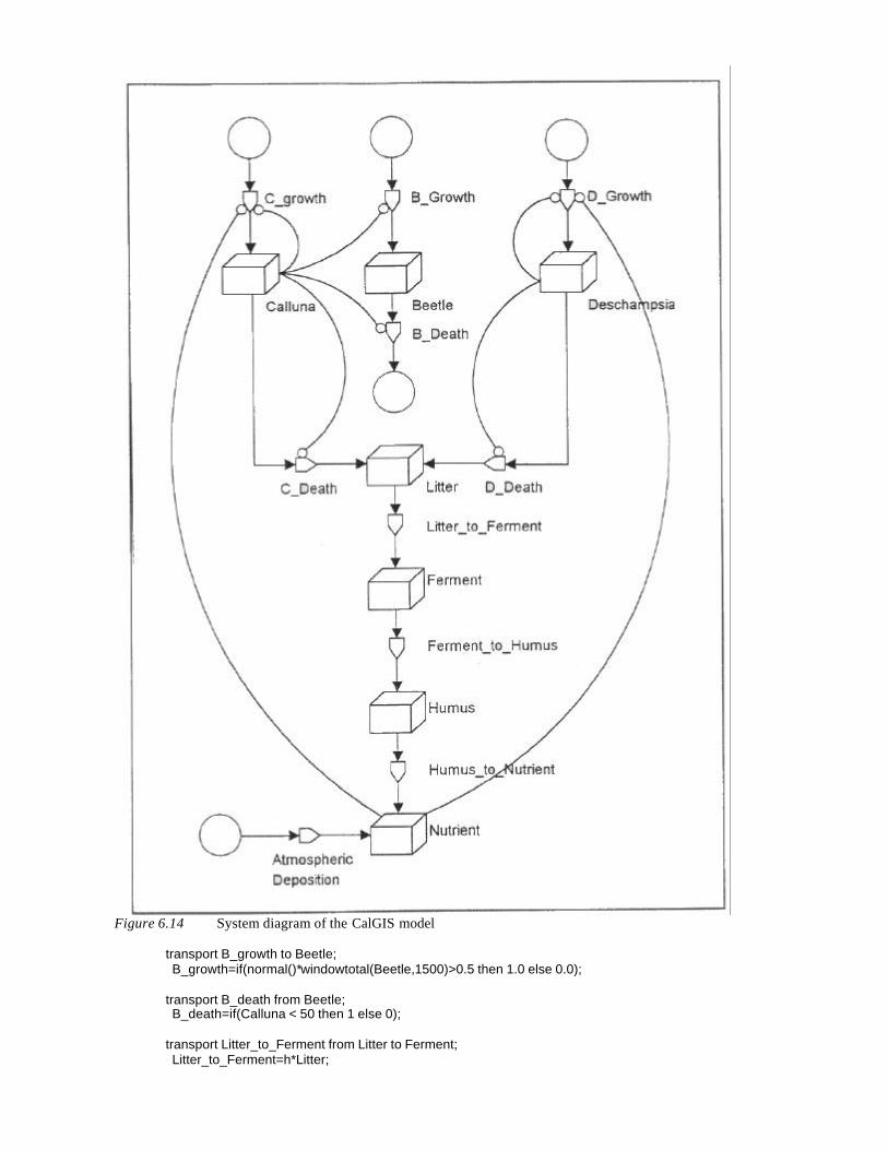
Figure 6.14 System diagram of the CalGIS model

transport B_growth to Beetle; B_growth=if(normal()*windowtotal(Beetle,1500)>0.5 then 1.0 else 0.0);

transport B_death from Beetle; B_death=if(Calluna < 50 then 1 else 0);

transport Litter_to_Ferment from Litter to Ferment; Litter_to_Ferment=h*Litter;

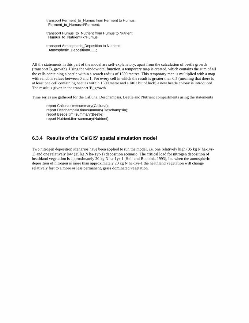
transport Ferment_to_Humus from Ferment to Humus; Ferment_to_Humus=i*Ferment;

transport Humus_to_Nutrient from Humus to Nutrient; Humus_to_Nutrient=k*Humus;

transport Atmospheric_Deposition to Nutrient; Atmospheric_Deposition=......;

All the statements in this part of the model are self-explanatory, apart from the calculation of beetle growth(transport B_growth). Using the windowtotal function, a temporary map is created, which contains the sum of allthe cells containing a beetle within a search radius of 1500 metres. This temporary map is multiplied with a mapwith random values between 0 and 1. For every cell in which the result is greater then 0.5 (meaning that there isat least one cell containing beetles within 1500 metre and a little bit of luck) a new beetle colony is introduced.The result is given in the transport 'B_growth'.

Time series are gathered for the Calluna, Deschampsia, Beetle and Nutrient compartments using the statements

report Calluna.tim=summary(Calluna);report Deschampsia.tim=summary(Deschampsia);report Beetle.tim=summary(Beetle);report Nutrient.tim=summary(Nutrient);

6.3.4 Results of the 'CalGIS' spatial simulation model

Two nitrogen deposition scenarios have been applied to run the model, i.e. one relatively high (35 kg N ha-1yr-1) and one relatively low (15 kg N ha-1yr-1) deposition scenario. The critical load for nitrogen deposition ofheathland vegetation is approximately 20 kg N ha-1yr-1 [Heil and Bobbink, 1993], i.e. when the atmosphericdeposition of nitrogen is more than approximately 20 kg N ha-1yr-1 the heathland vegetation will changerelatively fast to a more or less permanent, grass dominated vegetation.

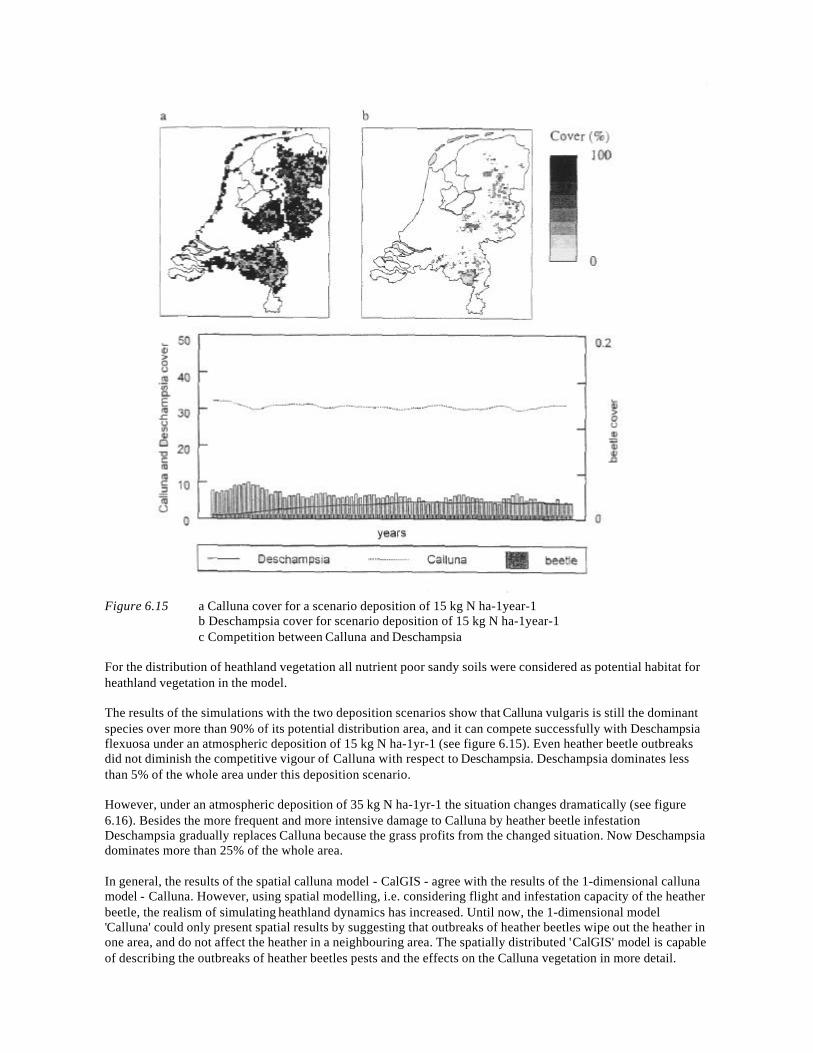
Figure 6.15 a Calluna cover for a scenario deposition of 15 kg N ha-1year-1b Deschampsia cover for scenario deposition of 15 kg N ha-1year-1c Competition between Calluna and Deschampsia

For the distribution of heathland vegetation all nutrient poor sandy soils were considered as potential habitat forheathland vegetation in the model.

The results of the simulations with the two deposition scenarios show that Calluna vulgaris is still the dominantspecies over more than 90% of its potential distribution area, and it can compete successfully with Deschampsiaflexuosa under an atmospheric deposition of 15 kg N ha-1yr-1 (see figure 6.15). Even heather beetle outbreaksdid not diminish the competitive vigour of Calluna with respect to Deschampsia. Deschampsia dominates lessthan 5% of the whole area under this deposition scenario.

However, under an atmospheric deposition of 35 kg N ha-1yr-1 the situation changes dramatically (see figure6.16). Besides the more frequent and more intensive damage to Calluna by heather beetle infestationDeschampsia gradually replaces Calluna because the grass profits from the changed situation. Now Deschampsiadominates more than 25% of the whole area.

In general, the results of the spatial calluna model - CalGIS - agree with the results of the 1-dimensional callunamodel - Calluna. However, using spatial modelling, i.e. considering flight and infestation capacity of the heatherbeetle, the realism of simulating heathland dynamics has increased. Until now, the 1-dimensional model'Calluna' could only present spatial results by suggesting that outbreaks of heather beetles wipe out the heather inone area, and do not affect the heather in a neighbouring area. The spatially distributed 'CalGIS' model is capableof describing the outbreaks of heather beetles pests and the effects on the Calluna vegetation in more detail.

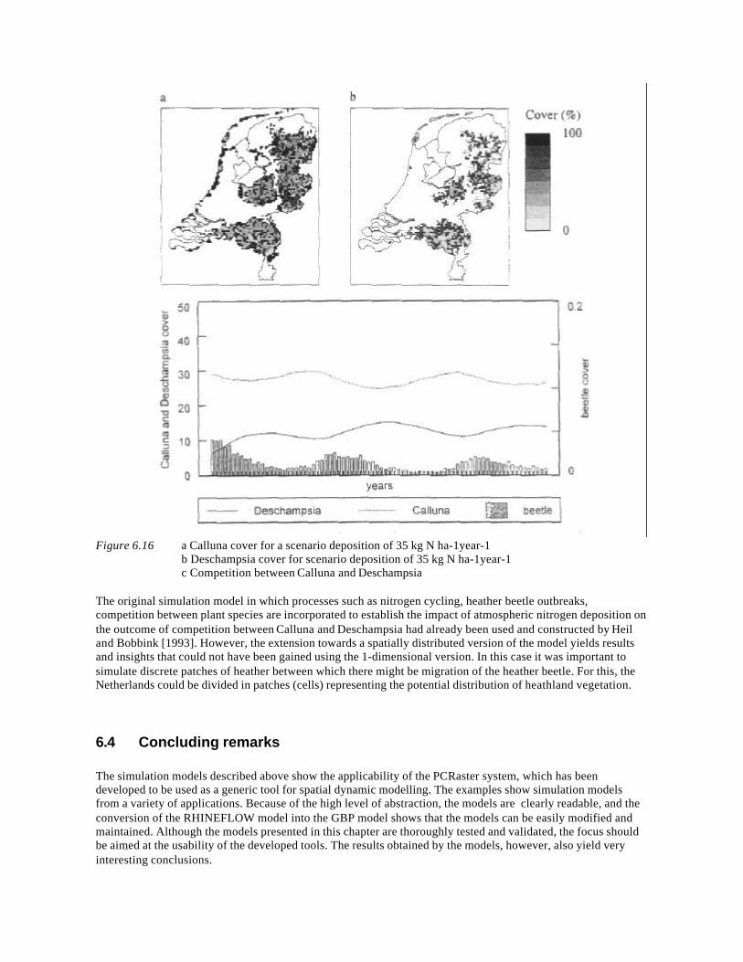
Figure 6.16 a Calluna cover for a scenario deposition of 35 kg N ha-1year-1b Deschampsia cover for scenario deposition of 35 kg N ha-1year-1c Competition between Calluna and Deschampsia

The original simulation model in which processes such as nitrogen cycling, heather beetle outbreaks,competition between plant species are incorporated to establish the impact of atmospheric nitrogen deposition onthe outcome of competition between Calluna and Deschampsia had already been used and constructed by Heiland Bobbink [1993]. However, the extension towards a spatially distributed version of the model yields resultsand insights that could not have been gained using the 1-dimensional version. In this case it was important tosimulate discrete patches of heather between which there might be migration of the heather beetle. For this, theNetherlands could be divided in patches (cells) representing the potential distribution of heathland vegetation.

6.4 Concluding remarks

The simulation models described above show the applicability of the PCRaster system, which has beendeveloped to be used as a generic tool for spatial dynamic modelling. The examples show simulation modelsfrom a variety of applications. Because of the high level of abstraction, the models are clearly readable, and theconversion of the RHINEFLOW model into the GBP model shows that the models can be easily modified andmaintained. Although the models presented in this chapter are thoroughly tested and validated, the focus shouldbe aimed at the usability of the developed tools. The results obtained by the models, however, also yield veryinteresting conclusions.

7 DISCUSSION AND RECOMMANDATIONS

7.1 Summary of research results

In the light of the results presented in chapters 4 through 6 this chapter gives answers to the research questionsthat were posed in chapter 1. The question to be answered was:

• Can we build a general purpose GIS with intrinsic dynamic modelling functionality, which can be used todevelop, apply and evaluate models for a large number of environmental processes?

Related research questions were:

• What are the advantages and disadvantages of the different techniques available for linking GIS anddynamic models?

• Can we classify the dynamic models currently used for physical geography, ecology and environmentalissues into useful sets of approaches and processes?

• Can we build general purpose tools to match these approaches and processes and are they capable of givingreasonable results for a variety of problems over a wide range of spatial scales?

• Are these tools sufficiently robust to be given to GIS users who a) are not expert modellers, and/or b) haveaccess to large amounts of pretty general data of mixed quality?

• For what kinds of dynamic modelling do they present a reasonable solution - where do they provide auseful supplement to existing methods?

• What should be the level of abstraction of these modules?

• Can we successfully model real-world problems in this GIS environment?

As discussed in chapter 2, a number of levels can be distinguished for linking GIS with dynamic models. Ofthese, the primitive linkages are currently the most widely used. Information exchange between model and GISis through a process of ad-hoc data conversion (low level integration) or is obtained by the establishment of acommon database structure supporting both GIS operations and model runs (medium level integration). Theseapproaches have in common that they separate the task of database management (GIS) from process description(creation of dynamic model executable) and application of the system (running the model, forecasting, scenarioanalysis and decision making using the model).

Current research and publications on the integration between GIS and dynamic models mainly focus on this lowand medium level integration (eg. Steyaert and Goodchild [1994] and Goodchild et al. [1993]). The dynamicmodel itself remains external to the GIS and, as Maidment [1993a, 1993b] states:

it does not seem productive to try to accomplish such simulations by intrinsic GIS functions, rather thesimulation should be kept separate from the GIS and just use GIS as a spatial data source

and

in this sense, the coupling of GIS and hydrologic models seems to be a logical direction, rather thanassuming that one can program hydrologic equations within GIS, a utility that will always be limited by the datamodel and operators available...

However, the separation between the model and GIS is troublesome, and listed as disadvantages are:• the ad-hoc development of low level linkages is time consuming and has to be repeated for new versions of

either the GIS or the model;• the low level linkage is hindered by redundancy and consistency problems due to the use of several

instances of the same database;

• the medium level integration requires a relative open GIS structure, which is not available in most currentGIS; and

• the model formulation remains at a relative low level.

The advantages of higher level integration become clear in this light. Although in theory these higher levelintegrations are handicapped by characteristics such as forcing the user into a straightjacket of model formulationand available numerical methods, the major advantage is the capability to build models relatively quickly and tobe able to change and manipulate process descriptions, control parameters and sub-models at a high level.Several authors recognise these advantages of a higher level linkage [Kemp, 1993a, Fedra, 1993a]. Kemp[1993a] argues for the development of a next generation spatial modelling languages. She lists the strategy forthe development of such a language as:• provide structures representing physical fields;• allow expression and manipulation of variables and data about continuous phenomena;• provide a syntax for incorporating primitive operations appropriate for environmental modelling with fields;• eliminate the necessity to consider the form of the spatial discretization whenever possible; and• the strategy should be capable of being incorporated into computer language implementations of

environmental models.

In general, the advantages of high level integration and the use of a spatial dynamic modelling language arelisted as: • there is a full integration of GIS functionality for manipulation of input, results and formulation of the

models;• no overhead for conversion between GIS and models and between individual models;• high level integration allows for rapid development of new models; and• high level integration allows for easy maintenance of models.

The major disadvantages of a high level approach are:• the current generation of commercial GIS does not fully support dynamic spatial modelling;• investment in development of tools and functionality is high;• the user is forced into a straightjacket of model formulation and numerical methods; and• lack of specialist insight may yield invalid model concepts and formulations: the user is fully responsible for

the model formulation.

This thesis has dealt with the development of a prototype of such a spatial dynamic modelling language for ahigh level integration of environmental models in GIS and evaluates the use of the new language.

High level languages provide a mechanism to express the problem in terms that conform with the concepts andideas related to the subject. They allow for a compact expression of the problem by obscuring implementationdetails. By hiding details, they allow the user to maintain an overview of the problem, which helps prevent errorsin developing solutions.

The development of a high level language for modelling spatially distributed dynamic processes begins with aclassification of approaches for this type of modelling into a limited number of categories, and subdivides eachapproach into separate generic tasks. Although the world of dynamic models for environmental processes iscurrently very dynamic, the methods can be standardised as using 1-dimensional, 2-dimensional and 3-dimensional approaches. A very useful description for processes in these domains is by using Systems Analysistechniques for describing mass balances (chapter 4). This yields a framework of compartments for mass storage,interconnected with a network of fluxes, transporting mass from one compartment to another. This frameworkhas been extended in this study to include spatial distributed compartments and transports, and to enable for theformulation of spatial distributed processes and internal redistribution of mass within the compartment. Thisframework yields a useful approach for describing a large number of processes encountered physical geography,hydrology and other environmental issues.

The next step in the development of a high level language for spatial integration is the implementation of thegeneric concepts derived from the analysis of specific individual models into functions: modules that are capableof performing the generic tasks from which the total model can be constructed. The developed languageimplements all the functionality necessary for constructing compartments and creating the network of transportsof mass between them.

The new language provides the functionality to create mass balance process models for physical geography. Thismeans that they can be used to model processes related to water movement through the landscape, soil andpollutant movement, processes such as erosion and deposition and growth and distribution processes inecosystems. The tools are very useful for implementing models of processes based on mass balanceconsiderations, but as other terms become more important, the functionality may be insufficient. The detaileddescription of the process of infiltration and vertical water movement through the soil is based on a detailedsimulation of the suction and changing permeability as a function of changing suction: generic tools may beinadequate for these processes. For these cases the system provides a mechanism for bypassing the SystemAnalysis mass balance approach and implementing models based on mathematical formulation of the model. Inaddition, the database can be accessed using a library written in the C-language, and this mechanism enables thedevelopment of special purpose models. An example of this latter approach is the development of LISEM, a soilerosion model integrated in GIS [De Roo et al., 1994].

The developed language provides a powerful mechanism for implementing many different kinds of dynamicmodels in GIS. This raises questions about the robustness of the language in hands of non-experiencedmodellers. This problem of robustness has been addressed in several sections in the thesis. On the one hand, thetools are helpful in designing and structuring the model, and shield the user from the details of theimplementation of the model. This enables the user to keep an overview of the model, instead of gaining insightin the number crunching of numerical solutions or the byte-level implications of changing model resolution. Onthe other hand, the user is still free to design whatever model he or she thinks is feasible and valid, and there isno mechanism or model expert knowledge in the system to point out weak or incorrect assumptions andmethods. The language helps to design, to structure and to implement models, but it does not prevent theimplementation of invalid model descriptions yielding incorrect results.

Since the model is integrated in GIS, all common GIS-tools for deriving new digital maps from a combination ofexisting maps and interpolation of coarse point-data to a fine resolution data-set are available. The tools areintegrated in a seamless way; extraction of necessary information can be done as part of the model description.Again a word of caution: the system cannot check whether relations assumed by the user have actual validity,and the responsibility for correctness is completely with the user.

The question whether we can actually analyse real world problems over a wide range of spatial scales withmodels built in this new GIS environment has been emphatically and positively answered in chapters 5 and 6.Important considerations relating to this question are which real world problems can be solved, and if there areproblems that cannot. Obviously, there are many problems that are not suitable to be solved with this type oftools. First, the use of these tools assumes that the considered problem can be modelled mathematically. Manyproblems are too vague or do not contain deterministic parts that lend themselves for mathematical modelling.Second, the approach assumes that the mass balance approach is a valid approach to solve the problem. Manyreal world problems cannot be described as mass balance problems, because they involve the solution ofchoosing between multiple alternatives to establish multiple objectives. However, as can be illustrated with theexamples in chapter 6, for a few of these problems the system provides a useful approach for simulating theprocesses that are important. The application of the tools is not only restricted to the processes of physicalgeography. As discussed in chapter 5 and 6, they also can be used for many different kinds of spatial problems,and the mass balance framework provides an approach that can be used for matters that are only slightly relatedto mass in a strict sense.

7.2 Recommendations for future research

This research provided for a set of tools to make the integration of computational models in a spatial databasesystem easier and more flexible. The spatial modelling language allows for the formulation of models for manyenvironmental processes. It allows for structuring the problem and developing computer programs that canactually simulate the processes. Chapter 2 provided a list of principles that should guide model development.These principles are related to model building and structuring, as well as to data availability, accuracy andtesting. Although the list is very clear in stating what a good model should be and should not be (it should not bemore complex than it needs to be, it should be testable, it should be accurate), it does not give any guidelines forhow to construct such a model. A model is never perfect, so there will be always the temptation to describe sub-processes in more detail, and increasing the complexibility of the model. Numerous examples can be given formodels that try to model too much, try to describe too much detail of processes and need more data than is

feasible to collect. The common approach is starting to interpolate a few point data so that they cover a completestudy area, or relate proxy estimates for important parameters to easy to measure data. This may easily lead to amodel in which there is no balance between the complexity of the process description, the accuracy of the inputdata and the required accuracy of the final results of the model. Clearly this approach leads to a waste of(limited) resources, and yields a situation in which the application of models is not as beneficial as it could be.More research should be done regarding structuring the problem and balancing the complexity of the steps andcomponents of the model building process.

The PCRaster system provides interfaces for tools for advanced interpolation and error propagation. These toolsallow for the evaluation of not only estimates of the expected results of spatial operations, but also for theanalysis of the variance in the results. An interpolation of some physical field from point data can beaccompanied by an estimate of the accuracy of the interpolation at each location in the physical field. However,the problem of propagation of errors or inaccuracies in the database through the process of dynamic modellinghas barely been touched. Questions regarding the relation between support size of measurements and effectiveparameter values for models need more attention. A sound theoretical framework for calibrating and validatinghigh resolution distributed models has not been set up yet. These are all question that should be addressed in thenear future, to give spatial modelling a more sound scientific foundation.

REFERENCES

ABBOTT, M.B., J.C. BATHURST, J.A. CUNGE, P.E. O'CONNEL & J. RASMUSSEN, (1986), Anintroduction to the European Hydrological System - Systeme Hydrologique Européen: SHE, 2. Structure of aphysically-based, distributed modeling system. Journal of Hydrology 87, pp. 61-77.

AERTS, R. (1989), Plant strategies and nutrient cycling in heathland ecosystems. PhD thesis, University ofUtrecht, The Netherlands.

AERTS, R. (1993), Biomass and nutrient dynamics of dominant plant species from heathlands. In: R. Aerts andG.W. Heil, eds., Heathlands: Patterns and processes in a changing environment. Geobotanie Series 20. Kluwer,Dordrecht.

ANDERSON, M.G. & C.C.M. ROGERS (1987), Catchment scale distributed models: a discussion of researchdirections. Progress in Physical Geography, 11, pp. 28-51.

ASHTON, C.H. & D. SIMMONS (1993), Multi-media: an integrated approach combining GIS within theframework of the Water Act 1989. In: K. Kovar & H.P. Nachtnebel, eds., Application of Geographic InformationSystems in Hydrology and Water Resources Management HydroGIS 1993. IAHS Publication No 211.

BAND, L.E. (1986), Topographic partition of watersheds with digital elevation models. Water ResourcesResearch 22, pp. 15-24.

BAUMGARTNER, A., E. REICHEL & G. WEBER (1983), Der Wasserhaushalt der Alpen. R. OldenbourgMünchen.

BEAR, J. & A. VERRUYT (1990), Modelling Groundwater Flow and Pollution. Kluwer Academic PublishersGroup.

BEASLEY, D.B. (1977), ANSWERS: A mathematical model for simulating the effects of land use andmanagement on water quality. PhD thesis, Purdue University, West-Lafayette, IN.

BERDOWKSI, J.J.M. (1987), The catastrophic death of Calluna vulgaris in Dutch heathlands. PhD thesis,University of Utrecht, The Netherlands.

BERDOWSKI, J.J.M. & R. ZEILINGA (1987), Transition from heathland to grassland, damaging effects of theheather beetle. Journal of Ecolology 75, pp. 159-175.

BERENDSE, F. & R. AERTS (1984), Competition between Erica tetralix L. and Molinia caerulea (L.) Moench.as affected by the availability of nutrients. Acta Oecologica/Oecologica Plantarum 5, pp. 3-14.

BERGSTRÖM, S. (1976), Development and application of a conceptual runoff model for Scandinaviancatchments. Dep. of Water resources engineering, Lund Institute of technology/ University of Lund Bulletinseries A No. 52.

BERNARD, M. (1939), Giving areal significance to hydrologic research on small areas. Headwaters Control andUse, Report of the Upstream Engineering Conference at Washington DC. US Department of Agriculture, SoilConservation Service, Washington DC, pp. 50-75.

BERRY, J.K. (1987), Fundamental operations in computer-assisted map analysis. International Journal ofGeographic Information Systems 2, pp. 119-136.

BEVEN, K.J. (1985), Distributed models. In: M.G. Anderson & T.P. Burt, eds., Hydrological forecasting. JohnWiley and Sons Ltd.

BEVEN, K.J. (1989), Changing ideas in hydrology - the case of physically based models. Journal of Hydrology105, pp. 157-172.

BEVEN, K.J. & A.B. BINLEY (1992), The future of distributed models: model calibration and uncertaintyprediction. Hydrological Processes 6, pp. 279-298.

BIERKENS, M.F.P. (1994), Complex confining layers: a stochastic analysis of hydraulic properties at variousscales. PhD thesis Department of Physical Geography, University of Utrecht, The Netherlands.

BIESHEUVEL, A. & C.J. HEMKER (1993), Groundwater modelling and GIS: integrating MICRO-FEM andILWIS. In: K. Kovar & H.P. Nachtnebel, eds., Application of Geographic Information Systems in Hydrologyand Water Resources Management HydroGIS 1993. IAHS Publication No 211.

BLANKWAARDT, H.F.H. (1977), The occurrence of the heather beetle (Lochmaea suturalis Thomson) in theNetherlands since 1915 (in Dutch). Entomologische berichten 37, pp. 34-40.

BOBBINK, R., G.W. HEIL & M. RAESSEN (1990), Atmospheric deposition and canopy exchange in heathlandecosystems. Dutch Priority Programme on Acidification, report project nr. 119; Department of Plant Ecologyand Evolutionary Biology, University of Utrecht, the Netherlands.

BRUNSTING, A.M.H. & G.W. HEIL (1985), The role of nutrients in the interactions between a herbivorousbeetle and some competing plant species in heathlands. Oikos 44, pp. 23-26.

BUIJSMAN, E., J.M. MAAS & W.A.H. ASMAN (1987), Anthropogenic NH3 emissions in Europe.Atmospheric Environment 21, pp. 1009-1022.

BURROUGH, P.A. (1986), Principles of Geographic Information Systems for Land Resources Assessment.Clarendon Press, Oxford.

BURROUGH, P.A. (1989), Matching spatial databases and quantitative models in land resource assessment. SoilUse and Management 5, pp. 3-8.

BURROUGH, P.A. (1992), Are GIS structures too simple minded? Computers and Geosciences 18, pp. 395-400.

BURROUGH, P.A. & A.U. FRANK (1995), Concepts and paradigms in spatial information: Are currentgeographic information systems truly generic? International Journal of Geographical Information Systems 9.

CHAIRAT, S. & J.W. DELLEUR (1993), Integrating a physically based hydrological model with GRASS. In:K. Kovar & H.P. Nachtnebel, eds., Application of Geographic Information Systems in Hydrology and WaterResources Management HydroGIS 1993. IAHS Publication No 211.

CHOW, V.T. (1988), Applied hydrology. McGraw-Hill series in water resources and environmental engineering.New York USA.

CHOW, V.T., D.R. MAIDMENT & L.W. MAYS (1988), Applied hydrology. McGraw-Hill series in waterresources and environmental engineering. McGraw-Hill Book Company, Singapore.

CHR/KHR (1976), Le Basin du Rhin / Das Rheingebiet. Monographie hydrologique / HydrologischerMonographie. Part A: texts, part B: tables, part C: maps and diagrams, CHR/KHR.

CHR/KHR (1995), Development and testing of a GIS based water balance model for the river Rhine drainagebasin. (Report in preparation)

CONWAY, D. (1993), Estimates of future runoff from the Blue Nile using a grid based hydrologic model. Paperpresented at the Third Technical Conference on Meteorology in Eastern and Southern Africa, Arusha, February22-26 1993.

COUCLELIS, H. (1992), People manipulate object (but cultivate fields). Beyond the raster-vector debate in GIS.In: Proceedings of the international conference on Theories and Methods of Spatio-Temporal Reasoning inGeographic Space. Pisa, Italy.

CRU (1992), World Climate Data disk. Climatic Research Unit, University of East Anglia, Norwich UK and theHadley Centre for Climatic Prediction and Research, Meteorological Office, Bracknell UK.

DE BOER, W. (1989), Nitrification in Dutch heathland soils. PhD thesis, Agricultural University ofWageningen. The Netherlands.

DECOURSEY, D.G. (1991), Mathematical models: research tools for experimental watersheds. In: D.S. Bowles& P.E. O'Connell, eds., Recent advances in the modelling of hydrologic systems. Kluwer Academic Publishers.

DE JONG, S.M. (1994), Applications of reflective remote sensing for land degradation studies in amediterranean environment. PhD thesis Department of Physical Geography, University of Utrecht, TheNetherlands.

DENNING, P.J. (1990), Modeling reality. American Scientist 76, pp. 495-498.

DOE (1987), Department of the Environment. Handling Geographic Information. HMSO, London.

DE ROO, A.P.J. (1993), Modelling surface runoff and soil erosion in catchments using GeographicalInformation Systems; Validity and applicability of the 'ANSWERS' model in two catchments in the loess area ofSouth-Limburg (The Netherlands) and one in Devon (UK). PhD thesis Department of Physical Geography,University of Utrecht, The Netherlands.

DE ROO, A.P.J., C.G. WESSELING, N.H.D.T. CREEMERS, R.J.E. OFFERMANS, C.J. RITSEMA & K. VANOOSTINDIE (1994), Lisem: a physically based hydrological and soil erosion model incorporated in a GIS. In:Proceedings of EGIS 1994.

DE SMIDT, J.T. (1977), Interaction of Calluna vulgaris and the heather beetle (Lochmaea suturalis). In: Tuxen,R., ed., Vegetation and Fauna.. J. Cramer, Vaduz, pp. 179-186.

DE SMIDT, J.T. (1979), Origin and destruction of Northwest European heath vegetation. In: O. Wilmans & R.Tuxen, eds., Werden und Vergehen von Pflanzengesellschaften. J. Cramer, Vaduz, pp. 411-435.

DUEKER, K.J. (1979), Land resource information systems: a review of fifteen years experience. Geo-Processing1, pp. 105-128.

EVANS, I.S. (1980), An integrated system of terrain analysis and slope mapping. Zeitschrift furGeomorphologie. Supplement 36, pp. 274-95.

FEDRA, K. (1993a), Distributed Models and Embedded GIS: Strategies and case studies of integration. SecondInternational Conference/Workshop on integrating geographic Information systems and EnvironmentalModelling. Breckenridge, September 1993.

FEDRA, K. (1993b), Models, GIS and expert systems, integrated water resources models. In: K. Kovar & H.P.Nachtnebel, eds., Application of Geographic Information Systems in Hydrology and Water ResourcesManagement HydroGIS 1993. IAHS Publication No 211.

FEDRA, K. (1993c), GIS and Environmental modeling. In: M.F. Goodchild, B.O. Parks & L.T. Steyaert, eds.,Environmental modelling with GIS. Oxford University Press.

FISHER, T.R. (1993), Integrated three dimensional geoscientific information system (GSIS) technologies forgroundwater and contaminant modelling. In: K. Kovar & H.P. Nachtnebel, eds., Application of GeographicInformation Systems in Hydrology and Water Resources Management HydroGIS 1993. IAHS Publication No211.

FORRESTER, J.W. (1968), Principles of systems. Text and workbook chapters 1 through 10. Wright-AllenPress, Inc. Cambridge, Massachusetts USA.

GAO, PENG, CIXIANG ZHAN & SUDHAKAR MENON (1993), An overview of Cell Based Modelling withGIS. Second International Conference/Workshop on integrating geographic Information systems andEnvironmental Modelling. Breckenridge, September 1993.

GHEZZI, C. & M. JAZAYERI, (1982), Programming language concepts, John Wiley and sons, New York.

GLEICK P.H. (1993), Water in Crisis, a guide to the world's fresh water resources. Oxford University Press,New York, USA.

GOODCHILD, M.F. (1992), Geographical data modeling. Computers and Geosciences 18, pp. 401-408.

GOODCHILD, M.F. (1993), Data Models and Data Quality: Problems and Prospects. In: M.F. Goodchild, B.O.Parks & L.T. Steyaert, eds., Environmental modelling with GIS. Oxford University Press.

GOODCHILD M.F., B.O. PARKS & L.T. STEYAERT Eds. (1993), Environmental modelling with GIS. OxfordUniversity Press.

GRAYSON, R.B., I.D. MOORE & T.A. MCMAHON (1992), Physically based hydrologic modeling - II. Is theconcept realistic? Water Resources Research 26, pp. 2659 - 2666.

GRAYSON, R.B., G. BLOSCHL, R.D. BARLING & I.D. MOORE (1993), Progress, scale and constraints tohydrological modelling in GIS. In: K. Kovar & H.P. Nachtnebel, eds., Application of Geographic InformationSystems in Hydrology and Water Resources Management HydroGIS 1993. IAHS Publication No 211.

GROENENDIJK, H. (1989), Estimation of waterholding-capacity of soils in Europe. The compilation of a soildataset. Simulation report CABO-TT 19, Centre of agrobiological research, Department of theoretical productionecology, Agricultural University, Wageningen, The Netherlands.

HEIL, G.W. & W.H. DIEMONT (1983), Raised nutrient levels change heathland into grassland. Vegetatio 53,pp. 113-120.

HEIL, G.W. (1984), Nutrients and the species composition of heathland. PhD thesis, University of Utrecht, TheNetherlands.

HEIL, G.W., D. VAN DAM & B. HEIJNE (1987), Catch of atmospheric deposition in relation to vegetationstructures of heathland. In: W.A.H. Asman & H.S.M.A. Diederen, eds., Ammonia and acidification. ProceedingsEURASAP symposium, 13 - 15 April 1987, RIVM, Bilthoven. The Netherlands, pp. 107-123.

HEIL, G.W. & M. BRUGGINK (1987), Competition between Calluna vulgaris (L.) Hull and Molinia caerulea(L.) Moench. Oecologia 73, pp. 105-108.

HEIL, G.W., M.J.A. WERGER, W. DE MOL, D. VAN DAM & B. HEIJNE (1988), Capture of atmosphericammonium by grassland canopies. Science 239, pp. 764-765.

HEIL, G.W. & R. BOBBINK (1993), "Calluna", a simulation model for evaluation of impacts of atmosphericnitrogen deposition on dry heathlands. Ecological Modelling 68 (1993), pp. 161-182.

HEUVELINK, G.B.M. (1993), Error propagation in quantitative spatial modelling applications in GeographicalInformation Systems. PhD-thesis Department of Physical Geography, University of Utrecht, The Netherlands.

HIGHMAN, B. (1967), A comparative study of programming languages. Computer monographs 2. MacDonaldLondon and Elsevier New York.

HILLEL, D. (1986), Modeling in soil physics: a critical review. Future Developments in Soil Science Research(A Collection of Soil Science Society of America Golden Anniversary Contributions). Presented at the AnnualMeeting, Soil Science Society of America, New Orleans, Louisiana.

HJEMFELT & AMERMAN (1980), The mathematical basin model of Merill Bernard. Procs of the HelsinkiSymposium. June 1980. IAHS publication 130.

HOEKSTRA, A. (1994), AQUA. An integrated tool for Water Policy Making. Contribution to UNEP WaterStudy. Draft report, RIVM, TUD.

HORN, B.K.P. (1981), Hill shading and reflectance map. Proceedings of the IEEE 69, pp. 1407-1417.

HORTON, R.E. (1945), Erosional development of streams and their drainage basins, hydrophysical approach toquantitative morphology. Bulletin of the Geolological Society of America 56, pp. 275-370.

HOOGENDOORN, J.H. (1993), Case study: optimalisatie waterbeheer in de regio Wierden/ Hoge Hexel. In:Gebruik van GIS bij grondwatermodellering, Rapporten en Nota's No. 32 van de CHO-TNO, 1993.

IPCC (1992), J.T. HOUGHTON, B.A. CALLENDER & S.K. VARNEY Eds., Climate Change 1992. TheSupplementary Report to the IPCC Scientific Assessment, Cambridge University Press.

JENSON, S.K. & J.O. DOMINGUE (1988), Extracting topographic structure from digital elevation data forgeographic information system analysis. Photogrammic Engineering and Remote Sensing 11, pp. 1593-1600.

JOHNSTONE, D. & W.P. CROSS (1949), Elements of applied hydrology. Ronald Press Co. New York.

JØRGENSEN, S.E. (1988), Fundamentals of Ecological Modelling. Developments in Environmental Modelling,9. Elsevier, Amsterdam, 1988.

KAMPS, P.T.W.J., T.N. OLSTHOORN & W.J. DROESEN (1993), Oecohydrologisch onderzoekLuchterduinen. In: Gebruik van GIS bij grondwatermodellering, Rapporten en Nota's 32 van de CHO-TNO,1993.

KELLER, R. (1958), Das Wasserangebot in der Bundesrepublik Deutschland. Forschungen zur DeutscheLandeskunde, pp. 103-105.

KEMP, K.K. (1993a), Environmental modelling and GIS; dealing with the spatial continuity. In: K. Kovar &H.P. Nachtnebel, eds., Application of Geographic Information Systems in Hydrology and Water ResourcesManagement HydroGIS 1993. IAHS Publication No 211.

KEMP, K.K. (1993b), Managing spatial continuity for integrating environmental models with GIS. SecondInternational Conference/Workshop on integrating geographic Information systems and EnvironmentalModelling. Breckenridge, September 1993.

KIRPICH, Z.P. (1940), Time of concentration of small agricultural watersheds. Civil Engineering 10, 362.

KLEMES, V. (1986a), Dilettantism in hydrology: transition or destiny? Water Resources Research 22, pp. 177-188.

KLEMES, V. (1986b), Operational testing of hydrological simulation models. Hydrological sciences journal -Des sciences Hydrologiques 31, pp. 13-24.

KWADIJK, J.C.J. (1993), The impact of climate change on the discharge of the River Rhine. PhD thesisDepartment of Physical Geography, University of Utrecht, The Netherlands.

LEAVESLY, G.H., P.J. RESTREPO, L.G. STANNARD, L.A. FRANKOSKI & A.M. SANTINS (1993), TheModular Modelling System MMS. Second International Conference/Workshop on integrating geographicInformation systems and Environmental Modelling. Breckenridge, September 1993.

MACMILLAN, R.A., P.A. FURLEY & R.G. HEALEY (1993), Using hydrological models and geographicinformation systems to assist with the management of surface water in agricultural landscapes. In: R. Haines-Young, D.R. Green & S.H. Cousins, eds., Landscape ecology and GIS. Taylor and Francis. London, 1993.

MAGUIRE, D.J. (1991), An overview and definition of GIS. In: Maguire, D.J., M.F. Goodchild & D.W. Rhind,eds., Geographical Information Systems: principles and applications. Longman, London.

MAIDMENT, D.R. (1993a), GIS and hydrologic modelling. In: M.F. Goodchild, B.O. Parks & L.T. Steyaert,eds., Environmental modelling with GIS. Oxford University Press.

MAIDMENT, D.R. (1993b), Environmental modeling with GIS. Second International Conference/Workshop onintegrating geographic Information systems and Environmental Modelling. Breckenridge, September 1993.

MAIDMENT, D.R. (1993c), Developing a spatially distributed unit hydrograph by using GIS. In: K. Kovar &H.P. Nachtnebel, eds., Application of Geographic Information Systems in hydrology and Water ResourcesManagement. Proceedings of the HydroGIS conference 1993. Vienna 1993. IAHS Publication No 211, pp. 181-192.

MARDIA, K.V. (1972), Statistics of directional data. Academic Press. London and New York.

MARK, D.M. (1984), Automated detection of drainage networks from digital elevation models. Cartographia 21,pp. 168-178.

MARK, D.M. (1988), Network models in geomorphology. In: M.G. Anderson, ed., Modelling ingeomorphological systems. John Wiley, Chichester, UK, pp. 73-97.

MARKS, D., J. DOZIER & J. FREW (1984), Automated basin delineation from digital elevation data. Geo-Processing 2, pp. 299-311.

MARTINEC, J., M. ROHRER & H. LANG (1992), Schneehöhn und Schneedecke, Hydrologische Atlas derSchweiz.

MCDONNELL, R.A. & W.D. MACMILLAN (1993), A GIS-based hierarchical simulation model for assessingthe impacts of large dam projects. In: K. Kovar & H.P. Nachtnebel, eds., Application of Geographic InformationSystems in Hydrology and Water Resources Management. Proceedings of the HydroGIS conference 1993,Vienna 1993. IAHS publication no 211, pp. 507-518.

MCDONALD, M.G. & A.W. HARBAUGH (1988), A modular three-dimensional finite difference ground-waterflow model. Techniques of water resources investigations of the USGS, Washington DC.

MOORE I.D. & M.F. HUTCHINSON (1991), Spatial extension of hydrologic process modeling. Proceedings ofthe International Hydrology and Water Resources Symposium. Perth, 2-4 October, Institute of Engineers ofAustralia, pp. 803-808.

MOORE, I.D., A. K. TURNER, J. P. WILSON, S. K. JENSON & L. E. BAND (1993), GIS and the land surface- subsurface process modeling. In: M.F. Goodchild, B.O. Parks & L.T. Steyaert, eds., Environmental modellingwith GIS. Oxford University Press.

MOORE, I.D. (1993), Hydrologic modelling and GIS. Second International Conference/Workshop onintegrating geographic Information systems and Environmental Modelling. Breckenridge, September 1993.

MORRIS, D. & R. HEERDEGEN (1988), Automatically derived catchment boundaries and channel networksand their hydrological applications. Geomorphology 1, pp. 131-141.

NASH, J.E. & J.V. SUTCLIFF (1970), River flow forecasting through conceptual models. Part 1-a discussion ofprinciples. Journal of Hydrology 10, pp. 282-290.

NYERGES, T.L. (1993), Understanding the scope of GIS: Its relation to environmental modeling. In: M.F.Goodchild, B.O. Parks & L.T. Steyaert, eds., Environmental modelling with GIS. Oxford University Press.

OLDEMAN, L.R. & H.T. VAN VELTHUYZEN (1991), Aspects and criteria of the agro-ecological zoningapproach of FAO. Working paper and preprint 91/07. International Soil Reference and Information CentreISRIC, Wageningen, the Netherlands.

OZEMY V.M., D.R. SMITH & A. SICHERMAN (1981), Evaluating computerized geographic informationsystems using decision analysis. Interfaces 11, pp. 92-98.

PARKER, H.D. (1988), The unique qualities of a geographic information system: a commentary. PhotogrammicEngineering and Remote Sensing 11, pp. 1547-1549.

PARKS, B.O. (1993), The need for integration. In: M.F. Goodchild, B.O. Parks & L.T. Steyaert, eds.,Environmental modelling with GIS. Oxford University Press.

PEBESMA, Edzer J. (1994), GSTAT User manual. Internal publication RIVM.

PEBESMA, E.J. & J.W. DE KWAADSTENIET (1994), Een landsdekkend beeld van de nederlandsegrondwaterkwaliteit op 5 tot 17 meter diepte in 1991. RIVM rapport no 714810014.

PRENTICE, I.C., M.T. SYKES & W. CRAMER (1993), A simulation model for the transient effects of climatechange on forest landscapes. Ecological Modeling 65, pp. 51-70.

RAPER, J. & D. LIVINGSTONE (1993), High level coupling of GIS and environmental process modelling.Second International Conference/Workshop on integrating geographic Information systems and EnvironmentalModelling. Breckenridge, September 1993.

RESOURCE ANALYSIS (1994), The impacts of climate change on the water balance of the Ganges-Brahmaputra and Yangtze basin. Report RA/94-160 prepared for TARGETS, RIVM.

REWERTS, C.C. & B.A. ENGEL (1991), ANSWERS on GRASS: Integrating a watershed simulation with aGIS. ASAE Paper 91 - 2621.

ROMANOWICZ, R., K. BEVEN, J. FREER & R. MOORE (1993), TOPMODEL as an application modulewithin GIS. In: K. Kovar & H.P. Nachtnebel, eds., Application of Geographic Information Systems inHydrology and Water Resources Management HydroGIS 1993. IAHS Publication No 211.

ROTMANS, J., M.B.A. VAN ASSELT, A.J. DE BRUIN, M.G.J. VAN ELZEN, J. DE GREEF, H.HILDERINK, A.Y. HOEKSTRA, M.A. JANSSEN, H.W. KÖSTER, W.J.M. MARTENS, L.W. NIESSEN &H.J.M. DE VRIES (1994), Global change and sustainable development. A modelling perspective for the nextdecade. Global Dynamics & Sustainable Development Programme GLOBO Report Series no. 4. RIVM Reportno. 461502004.

SCHÄDLER, B. (1985), Der Wasserhaushalt der Schweiz. Mitteilungen no.6. Bundesamt für Umwelschutz.Abteilung: Landeshydrologie, Bern/ Berne, Schweiz.

SMITH, T.R., S. MENON, J.L. STARR & J.E. ESTES (1987), Requirements and principles for theimplementation and construction of large-scale geographic information systems. International Journal ofGeographical Information Systems 1, pp. 13-31.

SOIL CONSERVATION SERVICE (1972), National Engineering Handbook, section 4, Hydrology, U.S. Deptof Agriculture, available from U.S. Government Printing Office, Washington DC, USA.

STEYAERT, L.T. & M.F. GOODCHILD (1994), Integrating geographic information systems and environmentalsimulation models: A status review. In: W.K. Michener, J.W. Brunt & S.G. Stafford, eds., EnvironmentalInformation Management and Analysis: Ecosystems to Global Scales. Taylor and Francis, 1994.

STRAHLER, A.N. (1960), Quantitative geomorphology of drainage basins and channel networks, section 4-II.In: V.T. Chow, ed., Handbook of Applied Hydrology, McGraw-Hill, New York USA, pp. 4-39 - 4-76.

STRAHLER, A.N. & A.H. STRAHLER (1987), Modern physical geography (3rd edition). John Wiley & sons,New York.

THORNTHWAITE, C.W. & J.R. MATHER (1957), Instructions and tables for computing potentialevapotranspiration and the water balance, Publications in climatology 10, pp. 183-243.

TOMLIN, C.D. (1980), The Map Analysis Package (draft manual). Yale School of Forestry and EnvironmentalStudies, New Haven, Connecticut.

TOMLIN C.D. (1983), Digital cartographic modelling techniques in environmental management. Doctoraldissertation, Yale University, School of Forestry and Environmental Studies, New Haven, Connecticut.

TOMLIN, C.D. (1990), Geographic information systems and cartographic modelling. Prentice Hall, N.J.

TOMLIN, C.D. & J.K. BERRY (1979), A mathematical structure for cartographic modelling in environmentalanalysis. Proceedings of the 39th Symposium. American Congress on Surveying and Mapping, Falls Church,Virginia, pp. 269-283.

VAN BREEMEN, N., P.A. BURROUGH, E.J. VELTHORTS, H.F. DOBBEN, T. DE WIT, T.B. DE RIDDER& H.F.R. REYNDERS (1982), Soil acidification from atmospheric ammonium sulphate in forest canopythroughfall. Nature 299, pp. 548-550.

VAN DAM, D., H.F. VAN DOBBEN, C.J.F. TER BRAAK & T. DE WIT (1986), Air pollution as possiblecause for the decline of some phanerogamic species in The Netherlands. Vegetatio 65, pp. 47-52.

VAN DER LEEDEN, F. (1990), The water encyclopedia. Lewis Publishers Inc. Chelsea, Michigan.

VAN DEURSEN, W.P.A. & J.C.J KWADIJK (1990), Using the Watershed tools for modelling the Rhinecatchment. In: Proceedings on the first European conference on G.I.S, pp. 254-263.

VAN DEURSEN, W.P.A. & J.C.J. KWADIJK (1993), RHINEFLOW: an integrated GIS water balance modelfor the river Rhine. In: K. Kovar & H.P. Nachtnebel, eds., Application of Geographic Information Systems inHydrology and Water Resources Management HydroGIS 1993. IAHS Publication No 211.

VAN DEURSEN, W.P.A. & G.W. HEIL (1993), Analysis of heathland dynamics using a spatial distributed GISmodel. Scripta Geobotanica 21 , pp. 17-28.

VAN DEURSEN, W.P.A. & C.G. WESSELING (1992), The PCRaster package. Technical report of theDepartment of Physical Geography, University of Utrecht, The Netherlands.

VAN DEURSEN, W.P.A. et al. (1992). Practicumhandleiding IGIS. Department of Physical Geography,University of Utrecht, The Netherlands.

VAN DEURSEN, W.P.A & R.A. MACMILLAN (1991), Internal report.

WIGLEY, T.M.L. & S.C.B. RAPER (1992), Implications for climate and sea level of revised IPCC emissionsscenarios, Nature 357, pp. 293-300.

ACKNOWLEDGEMENTS

This thesis would not have been finished without the continuing support and enthusiasm of my professor PeterBurrough. He not only guided me through the jungle of GIS, science and scientific writing, but he also managed toextent the STW project long enough so that, although I already quit my job at the University, I could finish thisthesis.

Many others were involved in the completion of this thesis. First, I want to thank Cees Wesseling. He provided mewith deep insights in things such diverse as structured programming, zaalvoetbal, movies, bars and beers and lots ofother items. Cees took the enormous task of explaining me why certain approaches I was very much in favour ofcould better be abandoned for simpler, more structured and definitely easier programmable approaches.

Jaap Kwadijk learned me everything I know about mountain climbing and the geomorphology of the Rhine basin.His project on climate change in the Rhine basin has been the first project ever carried out in PCRaster. Without hisideas, problems and friendship, PCRaster would have been a different program. Where we, normal people, can seeonly mountains of problems, he keeps on telling us that these mountains are full of bushaltes large enough to put thetip of your toe on. He has the strange habit of asking me the most difficult questions while I am hanging in the ropes,200 metres above the solid earth. Somehow, I learned to appreciate this behaviour.

Matthuscka Persijn is thanked for all the programming work she had to do for this project. Whenever I had a, what Ithought was a tremendous idea, Cees had to decide that it could be implemented, but Matthuscka was the one whohad to program it. Of course, my ideas were not always that bright, and Cees was not always right in his judgements.For Matthuscka, there was nobody left to take care of the problems.

Gerard Heuvelink, my roommate at the University explained me what random fields are, and he solved the statisticaland mathematical problems of the complete department. The discussions we had on the deterministic nature ofstochastic processes (or was it the other way around?) were very long and noisy, and still not finished.

Bob MacMillan from Edmonton, Canada has been a great support in the early stages of the project. It is thanks toBob that we have the largest number of pit removing options of any GIS available.

The vakgroep Fysische Geografie has offered me a nice place to work, and there is a list of persons always willing toaccompany me to pizza-dinners. These (former) colleagues and friends are Steven de Jong, Victor Jetten, Ad de Roo,Jos van Hees, Marc Bierkens, Ernst Jan Henkes, Edzer Pebesma, Hans Riezebos, Lodewijk Hazelhoff and many,many more.

My current employer Resource Analysis is thanked for the time made available to finish this project. The colleaguesof Resource Analysis supported me through this last year. Special thanks I owe to Jurgen Huizingh and Angelien vanBoxtel, for not only sharing blessings and successes, but also sharing the problems and difficulties. Gerrit Heil isthanked for introducing me into ecological modelling, discussing science and careers and commenting on the draftversions of the thesis.

Hoewel de steun van alle genoemde (en een heleboel niet genoemde) mensen onmisbaar is geweest voor hetoverleven van de jaren waarin ik dit proefschrift heb geschreven, is er een groep die ook onmisbaar is geweest in allejaren daarvoor. Riet, Miek, Pau, kinderen, Lied, Ciel, Bert, kinderen, Miech, Ditte, Tijs, Hans, Jack, Jaap, Maart,Eliz, kind, Koen, Suzan, kinderen, Koos bedankt voor alle steun, interresse en gezelligheid.

Tenslotte wil ik Marice bedanken. Zowel inhoudelijk als voor de uiteindelijke uitvoering (als bij het wandelen) heeftzij mij meer dan eens op het juiste pad teruggezet. Het is fijn iemand in de buurt te hebben die de stress van hetpromoveren van heel dichtbij kent. Overigens, gefeliciteerd met je overwinning...

CURRICULUM VITAE

Ik ben geboren op 10 februari 1960 in Zeist. In juni 1978 behaalde ik het diploma Atheneum-B aan descholengemeenschap 'De Breul' te Zeist. In 1979 begon ik met de studie Cultuurtechniek in Wageningen.Hiervoor behaalde ik in 1987 mijn doctoraal diploma. De belangrijkste vakken van de doctoraalstudie warenCultuurtechniek, Afvoerhydrologie en Informatica. In het kader van deze studie heb ik een zes maands stagegedaan bij de Klamath Indian tribe in de Verenigde Staten. Vanaf 1 maart 1988 ben ik als toegevoegdonderzoeker aangesteld aan de vakgroep Fysische Geografie van de Universiteit van Utrecht. De weerslag vanhet grootste deel van dit werk is te vinden in dit proefschrift. Naast het schrijven van dit proefschrift heb ik mijbezig gehouden met het GIS-onderwijs, en ben ik 3 maanden naar Canada geweest voor het bouwen van eenbodem informatie systeem. Vanaf mei 1991 ben ik werkzaam bij Resource Analysis in Delft.