Gridded Population of the World (GPW, v3) - Lessons Learned?

W. Christopher LenhardtCIESIN – Columbia University

27 May 2005

© 2005. The Trustees of Columbia University in the City of New York

Overview

• Background– A few words about CIESIN and SEDAC– What is GPW– How is it created– History of GPW

• A Few Applications

• What Have We Learned– Challenges Responses– Implications

And now few words from our sponsor…

• What is the Center for International Earth Science Information Network?– Part of the Earth Institute at Columbia University– Interdisciplinary mission to support research on human

interactions in the environment

• CIESIN’s Socieconomic Data and Applications Center (SEDAC) one of NASA’s Distributed Active Archive Centers (DAACs), part of NASA’s Earth Observing Data and Information System.

We have a pretty good idea how many people there are…

“USA Today has come out with a new survey:apparently, three out of every

four people make up 75% of the population.”

-- David Letterman

However: We’d like to know where are the people

• The “Where’s Waldo?” problem– (And Waldo 在哪里是 ? and Wo ist Walter? and Où

est Waldo ? and Где Waldo? and so on…

GPW: Inputs

• Inputs are relative simple– Population of administrative areas, usually in census years– Spatial boundaries of administrative areas

• Population and boundary data must match – Best available & ‘match-able’ data are used

• Matching the inputs to one another is not as easy as it might seem– Boundaries change often and come in different scales– Population data may not match boundaries

• We may have population values for different years at different levels (e.g., district-level one year, state-level another)

– Population and boundary data may not match themselves

Source Data Characteristics

• Commercial, government and other institutional sources– over 150 sources– roughly 100 data suppliers

• Information is often missing– Projection of spatial data– Relationship between new and old administrative units– Basic metadata

• Implications: – Educated guesswork is sometimes the best we can do!– Limits on redistribution of input data

• We haven’t made redistribution of the inputs a priority• In some instances, the data we have are propriety so that we cannot re-disseminate

them• Even where we could, our notes on assumptions used to clean the input shape files are

often less clean than we would like for a public release project

What do the input data look like?

• Population data:– Paper tables – Numbers in digital reports (e.g., pdf)– Digital tables (e.g., xls)– In digital file attached to spatial data (e.g., shp file)

• Spatial data– Paper maps– Digital images– Digital maps

Data acquisition

• From known sources– Established data providers (without personal connection)

• Census Bureaus

– Rely on a network on like-minded associates• UN agencies, The World Bank, Regional institutions, In-country

collaborators

• Alternative sources– Email requests and occasional phone calls to census offices and

geographic units of governments in far away places– Tourist and assorted other maps occasionally valuable for island

nations– Opportunistic

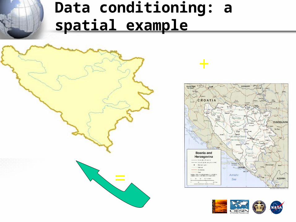
Data conditioning: a spatial example

+

=

Spatial data preparation

• Clean boundaries– E.g., remove slivers

• Make them consistent across borders and coasts– Use international standard—the Digital Chart of the World

(DCW) — with exceptions• Europe—most spatially data supplied by one agency (SABE –

Seamless Administrative Boundary for Europe) and all international boundaries are internally consistent

– Coastlines matched to DCW, except where much higher quality data are supplied

• E.g., Indonesia• Data table needs to include the same variables, with the same variable

names, formats, etc.

Data conditioning: A population example

Places highlighted in yellow are new municipiosNeed to find where they came from & their pop size

Use on-line atlases or newer maps, when availableAdd new pop to unit of origin or allocate old population to new unit proportionally.

After the data are conditioned

• That is, there is a clean, consistent, spatial data file with a table of data with the expected content in the expected form—that is, iso.shp

–— it’s time to grid!

Gridding Algorithm

• Proportional allocation used to spread the population over grid cells

• Virtually all data work completed on vector data– Gridding is the last step

• National grids created, global grids assembled by adding national grids together– Country grids are created with collars so that they start

and end on even degrees; therefore the assembly of the grids without interpolation is possible

– Replacement of country-specific grids feasible

Area 16.1 km2

Pop = 628.5 * 16.110,118.9 persons

Area 2.6 km2

Pop = 628.5 * 2.61,634.1persons

Area 0.05 km2

Pop = 628.5 * 0.0531.4 persons

Cell by cell…

Version (pub) GPW v1 (1995) GPW v2 (2000) GPW v3 (2003)

Estimates for 1994 1990, 1995 1990, 1995, 2000

Input units 19,000 127,000 ~ 350,000 globally

102,000 units in Africa

GPW History: Ten Years of Progress

Lots of hard work, was it worth it?

) /() ( unitsofnumberareacountryMean resolution in km =

Table 2.

Level Used

Frequency Average

Resolution

Frequency Average

Resolution

0 20 29 461 68 71 792 88 56 593 36 25 314 4 5 765 1 13 --? 2 ? ?

Overall 47 60

GPW 3

8119102

GPW 2

4163

GPW limitations

• Population estimation is not time-varying– Census measure, e.g., usual residence– One point in time, not

• where do work

• how do you commute

• where might you spend significant time

• Resolution may be too coarse for some applications– E.g., estimates of coastal population within a 50 km buffer

• No formal delineation of urban areas or other features– except those that may be deduced from population density– No other demographic variables (age, gender, etc)

Applications of GPW

• How many people live near the coast

• How many people live next to volcanoes

• Relationships between population and ecosystems

• Incorporated into a model to estimate potential risks for space vehicle re-entry

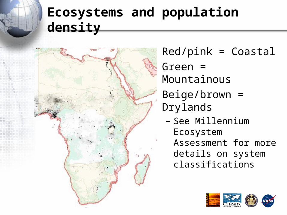
Ecosystems and population density

• Red/pink = Coastal

• Green = Mountainous

• Beige/brown = Drylands– See Millennium

Ecosystem Assessment for more details on system classifications

What have we learned and what does it mean for users

• Challenges

• Responses

• Implications for Users

Challenges/Responses

• Lots and lots of files both inputs and outputs -> How to manage? How to document?

• Granularity– At what level should be provide metadata: global,

continental, national, sub-national?

• Continued need for access to the best available data– Humanitarian and other types of disasters highlight

the need to provide better access to existing data sources and may serve to ‘shake loose’ previously unavailable data at least on a temporary basis

Challenges/Responses (cont.)

• Capture – Data analysis gap (!)– User Workshop results

• Provide an integrated information system for users to access– Data– Metadata and documentation– Graphics– Citations

• Need for ‘continuous process improvement’ in terms of data management and documentation– Work as a team, involve data managers, documentation specialists,

archival specialists all along the way

Implications for Users

• Better get it right given the potential uses for things like hazard risk estimation and other policy questions

• Data quality review – Review process (alpha -> beta -> production)– Rely on our users to discover errors

• More and better data– Development of derivative products– Continued need to work on cross-national research to harmonize

social science data (methods, variable operationalization, and so on)

• Need to think more how ‘cyberinfrastructure’ can further the social science and interdisciplinary research agendas (integrating IT and science for a new paradigm for scientific research)– Address issues of ontologies, epistemological differences, scale and

resolution

Thank you!

http://sedac.ciesin.columbia.edu/gpw