Grzegorz Łukaszewicz Piotr Kalita Navier– Stokes Equations

Advances in Mechanics and Mathematics 34

Grzegorz ŁukaszewiczPiotr Kalita

Navier–Stokes EquationsAn Introduction with Applications

Advances in Mechanics and Mathematics

Volume 34

Series Editors:David Y. Gao, Virginia Polytechnic Institute and State UniversityTudor Ratiu, École Polytechnique Fédérale

Advisory Board:Ivar Ekeland, University of British ColumbiaTim Healey, Cornell UniversityKumbakonam Rajagopal, Texas A&M UniversityDavid J. Steigmann, University of California, Berkeley

More information about this series at http://www.springer.com/series/5613

http://www.springer.com/series/5613

Grzegorz Łukaszewicz • Piotr Kalita

Navier–Stokes EquationsAn Introduction with Applications

123

Grzegorz ŁukaszewiczFaculty of Mathematics,

Informatics, and MechanicsUniversity of WarsawWarszawa, Poland

Piotr KalitaFaculty of Mathematics and Computer

ScienceJagiellonian University in KrakowKrakow, Poland

ISSN 1571-8689 ISSN 1876-9896 (electronic)Advances in Mechanics and MathematicsISBN 978-3-319-27758-5 ISBN 978-3-319-27760-8 (eBook)DOI 10.1007/978-3-319-27760-8

Library of Congress Control Number: 2015960205

© Springer International Publishing Switzerland 2016This work is subject to copyright. All rights are reserved by the Publisher, whether the whole or part ofthe material is concerned, specifically the rights of translation, reprinting, reuse of illustrations, recitation,broadcasting, reproduction on microfilms or in any other physical way, and transmission or informationstorage and retrieval, electronic adaptation, computer software, or by similar or dissimilar methodologynow known or hereafter developed.The use of general descriptive names, registered names, trademarks, service marks, etc. in this publicationdoes not imply, even in the absence of a specific statement, that such names are exempt from the relevantprotective laws and regulations and therefore free for general use.The publisher, the authors and the editors are safe to assume that the advice and information in this bookare believed to be true and accurate at the date of publication. Neither the publisher nor the authors orthe editors give a warranty, express or implied, with respect to the material contained herein or for anyerrors or omissions that may have been made.

Printed on acid-free paper

This Springer imprint is published by Springer NatureThe registered company is Springer International Publishing AG Switzerland

To Renata, Agata, and Jacek, with love(Grzegorz)

To my beloved wife Kasia(Piotr)

Preface

Admittedly, as useful a matter as the motion of fluid and relatedsciences has always been an object of thought. Yet until this dayneither our knowledge of pure mathematics nor our command ofthe mathematical principles of nature have a successfultreatment.

–Daniel Bernoulli

Incompressible Navier–Stokes equations describe the dynamic motion (flow) ofincompressible fluid, the unknowns being the velocity and pressure as functions oflocation (space) and time variables. To solve those equations would mean to predictthe behavior of the fluid under knowledge of its initial and boundary states. Theseequations are one of the most important models of mathematical physics. Althoughthey have been a subject of vivid research for more than 150 years, there are stillmany open problems due to the nature of nonlinearity present in the equations.The nonlinear convective term present in the equations leads to phenomena suchas eddy flows and turbulence. In particular the question of solution regularity forthree-dimensional problem was appointed by Clay Mathematics Institute as one ofthe Millennium Problems, that is, the key problems in modern mathematics. This is,on one hand, due to the fact that the problem remains challenging and fascinatingfor mathematicians and, on the other hand, that the applications of the Navier–Stokes equations range from aerodynamics (drag and lift forces), through designof watercrafts and hydroelectric power plants, to the medical applications of themodels of flow of blood in vessels.

This book is aimed at a broad audience of people interested in the Navier–Stokesequations, from students to engineers and mathematicians involved in the researchon the subject of these equations.

It originated in part from a series of lectures of the first author given over the past15 years at the Faculty of Mathematics, Informatics and Mechanics of the Universityof Warsaw; at summer schools at UNICAMP, Campinas, Brasil; and at UniversitéJean Monnet, Saint-Etienne, France. The lectures were based on the leading bookson the then young theory of infinite dimensional dynamical systems, focused onmathematical physics, in particular, on Temam [220]; Chepyzhov and Vishik [61];Doering and Gibbon [88]; Foias, Manley, Rosa, and Temam [99]; and Robinson[197].

vii

viii Preface

The lectures at the Mathematics Faculty of the University of Warsaw were alsoattended by students and PhD students from the Faculty of Physics and Facultyof Geophysics, and it became clear that a routine mathematical lecture had to beextended to include additional aspects of hydrodynamics. Some students asked for“more physics and motivation” and “more real applications”; others were mainlyinterested in the mathematics of the Navier–Stokes equations, and yet others wouldlike to see the Navier–Stokes equations in a more general context of evolutionequations and to learn the theory of infinite dimensional dynamical systems on theresearch level. These several aspects of hydrodynamics well suited the tastes andinterests of the lecturer, and also the second author was welcomed to join the projectof the book at a later stage.

In consequence, the audience of the book is threesome:

Group I: Mathematicians, physicists, and engineers who want to learn about theNavier–Stokes equations and mathematical modeling of fluidsGroup II: University teachers who may teach a graduate or PhD course on fluidmechanics basing on this book or higher-level students who start research on theNavier–Stokes equationsGroup III: Researchers interested in the exchange of current knowledge ondynamical systems approach to the Navier–Stokes equations

Although, in principle, all these three groups can find interest in all chapters ofthe book, Chaps. 2–7 are primarily targeted at Group I, Chaps. 3, 4, 7, 8, 11, and 12aimed mainly at Group II, and Chaps. 7–16 for Group III.

For a reader with reasonable background on calculus, functional analysis, andtheory of weak solutions for PDEs, the whole book should be understandable.

The book was planned to be a monograph which could also be used as a textbookto teach a course on fluid mechanics or the Navier–Stokes equations. Typicalcourses could be “Navier–Stokes equations”, “partial differential equations”, “fluidmechanics”, “infinite dimensional dynamics systems.” To this end many chaptersof this book include exercises. Moreover, we did not restrain ourselves to includea number of figures to liven the text and make it more intuitive and less formal.We believe that the figures will be helpful. Special care was undertaken to keep theindividual chapters self-contained as far as possible to allow the reader to read thebook linearly (in linear portions). That demanded several small repetitions here andthere.

To understand the first chapters of this book, just the basic knowledge oncalculus, that can be learned from any calculus textbook, should be enough.

The book is planned to be self-contained, but, to understand its last chapters,some knowledge from a textbook like “Partial Differential Equations” by L.C. Evans(which contains all necessary knowledge on functional analysis and PDEs) wouldbe helpful. Each chapter contains an introduction that explains in simple words thenature of presented results and a section on bibliographical notes that will place itin the context of past and current research.

Preface ix

Several people greatly contributed, knowingly or not knowingly, to the creationof the book. Our thanks go to our colleagues and collaborators: Guy Bayada, MahdiBoukrouche, Thomas Caraballo, José Langa, Pepe Real, James Robinson etc.

The first author is grateful to Guy Bayada who introduced him to the problemsof lubrication theory and flows in narrow films during his visits at INSA, Lyon,and to Mahdi Boukrouche with whom he collaborated for several years on thissubject. Thomas Caraballo, José Langa, and Pepe Real introduced him to the subjectof pullback attractors during his visit at the University of Seville. Thanks for theopportunity to give the summer courses in Campinas and Saint-Etienne go to MarcoRojas-Medar and Mahdi Boukrouche, respectively. Many thanks go also to ChunyouSun, Meihua Yang, and Yongqin Xie for their kind invitation of the first author togive several lectures at the University of Lanzhou, then at Huazhong Universityof Science and Technology in Wuhan and at The University in Changsha, China,in June 2013. Inspirational discussions and exchange of ideas with these Chinesefriends, including also Qingfeng Ma and Yuejuan Wang, contributed to the form ofthe last chapters of the book.

The research group at Jagiellonian University with their leader, StanisławMigórski, greatly motivated the authors as regards contact problems. The secondauthor owes a lot to his colleagues and teachers from Jagiellonian University; hewould like to express his thanks especially to Zdzisław Denkowski and StanisławMigórski. He would also like to thank Robert Schaefer who first introduced to himthe topics of fluid mechanics. He is also grateful for inspiring discussions in the fieldof contact mechanics to his collaborators from the University of Perpignan, MirceaSofonea and Mikaël Barboteu.

We would like to thank Wojciech Pociecha for his help with the preparation ofthe figures.

The work was in part supported by the National Science Center of Poland underthe Maestro Advanced Project no. DEC-2012/06/A/ST1/00262.

Finally, we express our gratitude to the AMMA Series editor, David Y. Gao, andto Marc Strauss and the editors of Springer Publishing House for their care andencouragement during the preparation of the book.

Warszawa, Poland Grzegorz ŁukaszewiczKraków, Poland Piotr KalitaOctober 2015

Contents

1 Introduction and Summary . . . . . . . . . . . . . . . . . . . . . . . . . . . . . . . . . . . . . . . . . . . . . . . 1

2 Equations of Classical Hydrodynamics . . . . . . . . . . . . . . . . . . . . . . . . . . . . . . . . . . 112.1 Derivation of the Equations of Motion . . . . . . . . . . . . . . . . . . . . . . . . . . . . . . 112.2 The Stress Tensor. . . . . . . . . . . . . . . . . . . . . . . . . . . . . . . . . . . . . . . . . . . . . . . . . . . . . 202.3 Field Equations . . . . . . . . . . . . . . . . . . . . . . . . . . . . . . . . . . . . . . . . . . . . . . . . . . . . . . . 222.4 Navier–Stokes Equations . . . . . . . . . . . . . . . . . . . . . . . . . . . . . . . . . . . . . . . . . . . . 232.5 Vorticity Dynamics . . . . . . . . . . . . . . . . . . . . . . . . . . . . . . . . . . . . . . . . . . . . . . . . . . . 242.6 Thermodynamics . . . . . . . . . . . . . . . . . . . . . . . . . . . . . . . . . . . . . . . . . . . . . . . . . . . . . 262.7 Similarity of Flows and Nondimensional Variables . . . . . . . . . . . . . . . . 282.8 Examples of Simple Exact Solutions . . . . . . . . . . . . . . . . . . . . . . . . . . . . . . . . 312.9 Comments and Bibliographical Notes. . . . . . . . . . . . . . . . . . . . . . . . . . . . . . . 36

3 Mathematical Preliminaries . . . . . . . . . . . . . . . . . . . . . . . . . . . . . . . . . . . . . . . . . . . . . . . 393.1 Theorems from Functional Analysis . . . . . . . . . . . . . . . . . . . . . . . . . . . . . . . . 393.2 Sobolev Spaces and Distributions . . . . . . . . . . . . . . . . . . . . . . . . . . . . . . . . . . . 443.3 Some Embedding Theorems and Inequalities. . . . . . . . . . . . . . . . . . . . . . . 483.4 Sobolev Spaces of Periodic Functions . . . . . . . . . . . . . . . . . . . . . . . . . . . . . . 543.5 Evolution Spaces and Their Useful Properties . . . . . . . . . . . . . . . . . . . . . . 613.6 Gronwall Type Inequalities . . . . . . . . . . . . . . . . . . . . . . . . . . . . . . . . . . . . . . . . . . 673.7 Clarke Subdifferential and Its Properties . . . . . . . . . . . . . . . . . . . . . . . . . . . . 703.8 Nemytskii Operator for Multifunctions . . . . . . . . . . . . . . . . . . . . . . . . . . . . . 743.9 Clarke Subdifferential: Examples . . . . . . . . . . . . . . . . . . . . . . . . . . . . . . . . . . . 773.10 Comments and Bibliographical Notes. . . . . . . . . . . . . . . . . . . . . . . . . . . . . . . 81

4 Stationary Solutions of the Navier–Stokes Equations . . . . . . . . . . . . . . . . . . 834.1 Basic Stationary Problem . . . . . . . . . . . . . . . . . . . . . . . . . . . . . . . . . . . . . . . . . . . . 83

4.1.1 The Stokes Operator . . . . . . . . . . . . . . . . . . . . . . . . . . . . . . . . . . . . . . . . 844.1.2 The Nonlinear Problem. . . . . . . . . . . . . . . . . . . . . . . . . . . . . . . . . . . . . 864.1.3 Other Topological Methods to Deal with the

Nonlinearity . . . . . . . . . . . . . . . . . . . . . . . . . . . . . . . . . . . . . . . . . . . . . . . . . 904.2 Comments and Bibliographical Notes. . . . . . . . . . . . . . . . . . . . . . . . . . . . . . . 93

xi

xii Contents

5 Stationary Solutions of the Navier–Stokes Equations with Friction . . 955.1 Problem Formulation. . . . . . . . . . . . . . . . . . . . . . . . . . . . . . . . . . . . . . . . . . . . . . . . . 955.2 Friction Operator and Its Properties . . . . . . . . . . . . . . . . . . . . . . . . . . . . . . . . . 965.3 Weak Formulation . . . . . . . . . . . . . . . . . . . . . . . . . . . . . . . . . . . . . . . . . . . . . . . . . . . . 985.4 Existence of Weak Solutions for the Case of Linear

Growth Condition . . . . . . . . . . . . . . . . . . . . . . . . . . . . . . . . . . . . . . . . . . . . . . . . . . . . 1035.5 Existence of Weak Solutions for the Case of Power

Growth Condition . . . . . . . . . . . . . . . . . . . . . . . . . . . . . . . . . . . . . . . . . . . . . . . . . . . . 1075.6 Comments and Bibliographical Notes. . . . . . . . . . . . . . . . . . . . . . . . . . . . . . . 109

6 Stationary Flows in Narrow Films and the Reynolds Equation . . . . . . . 1116.1 Classical Formulation of the Problem . . . . . . . . . . . . . . . . . . . . . . . . . . . . . . . 1116.2 Weak Formulation and Main Estimates . . . . . . . . . . . . . . . . . . . . . . . . . . . . . 1146.3 Scaling and Uniform Estimates . . . . . . . . . . . . . . . . . . . . . . . . . . . . . . . . . . . . . . 1216.4 Limit Variational Inequality, Strong Convergence,

and the Limit Equation . . . . . . . . . . . . . . . . . . . . . . . . . . . . . . . . . . . . . . . . . . . . . . . 1256.5 Remarks on Function Spaces . . . . . . . . . . . . . . . . . . . . . . . . . . . . . . . . . . . . . . . . 1286.6 Strong Convergence of Velocities and the Limit Equation . . . . . . . . . 1346.7 Reynolds Equation and the Limit Boundary Conditions . . . . . . . . . . . 1376.8 Uniqueness . . . . . . . . . . . . . . . . . . . . . . . . . . . . . . . . . . . . . . . . . . . . . . . . . . . . . . . . . . . 1416.9 Comments and Bibliographical Notes. . . . . . . . . . . . . . . . . . . . . . . . . . . . . . . 142

7 Autonomous Two-Dimensional Navier–Stokes Equations . . . . . . . . . . . . . 1437.1 Navier–Stokes Equations with Periodic Boundary Conditions . . . . 1437.2 Existence of the Global Attractor: Case of Periodic

Boundary Conditions. . . . . . . . . . . . . . . . . . . . . . . . . . . . . . . . . . . . . . . . . . . . . . . . . 1517.3 Convergence to the Stationary Solution: The Simplest Case. . . . . . . 1577.4 Convergence to the Stationary Solution for Large Forces . . . . . . . . . . 1597.5 Average Transfer of Energy. . . . . . . . . . . . . . . . . . . . . . . . . . . . . . . . . . . . . . . . . . 1637.6 Comments and Bibliographical Notes. . . . . . . . . . . . . . . . . . . . . . . . . . . . . . . 166

8 Invariant Measures and Statistical Solutions . . . . . . . . . . . . . . . . . . . . . . . . . . . . 1698.1 Existence of Invariant Measures . . . . . . . . . . . . . . . . . . . . . . . . . . . . . . . . . . . . . 1698.2 Stationary Statistical Solutions . . . . . . . . . . . . . . . . . . . . . . . . . . . . . . . . . . . . . . 1768.3 Comments and Bibliographical Notes. . . . . . . . . . . . . . . . . . . . . . . . . . . . . . . 181

9 Global Attractors and a Lubrication Problem . . . . . . . . . . . . . . . . . . . . . . . . . . 1839.1 Fractal Dimension . . . . . . . . . . . . . . . . . . . . . . . . . . . . . . . . . . . . . . . . . . . . . . . . . . . . 1839.2 Abstract Theorem on Finite Dimensionality and an Algorithm. . . . 1859.3 An Application to a Shear Flow in Lubrication Theory . . . . . . . . . . . . 193

9.3.1 Formulation of the Problem . . . . . . . . . . . . . . . . . . . . . . . . . . . . . . . . 1939.3.2 Energy Dissipation Rate Estimate . . . . . . . . . . . . . . . . . . . . . . . . . 1969.3.3 A Version of the Lieb–Thirring Inequality . . . . . . . . . . . . . . . . 2009.3.4 Dimension Estimate of the Global Attractor . . . . . . . . . . . . . . 201

9.4 Comments and Bibliographical Notes. . . . . . . . . . . . . . . . . . . . . . . . . . . . . . . 204

Contents xiii

10 Exponential Attractors in Contact Problems . . . . . . . . . . . . . . . . . . . . . . . . . . . . 20710.1 Exponential Attractors and Fractal Dimension . . . . . . . . . . . . . . . . . . . . . 20710.2 Planar Shear Flows with the Tresca Friction Condition . . . . . . . . . . . . 211

10.2.1 Problem Formulation . . . . . . . . . . . . . . . . . . . . . . . . . . . . . . . . . . . . . . . 21110.2.2 Existence and Uniqueness of a Global in Time Solution . 21810.2.3 Existence of Finite Dimensional Global Attractor . . . . . . . . 22210.2.4 Existence of an Exponential Attractor . . . . . . . . . . . . . . . . . . . . . 229

10.3 Planar Shear Flows with Generalized TrescaType Friction Law . . . . . . . . . . . . . . . . . . . . . . . . . . . . . . . . . . . . . . . . . . . . . . . . . . . . 23110.3.1 Classical Formulation of the Problem . . . . . . . . . . . . . . . . . . . . . 23110.3.2 Weak Formulation of the Problem . . . . . . . . . . . . . . . . . . . . . . . . . 23310.3.3 Existence and Properties of Solutions . . . . . . . . . . . . . . . . . . . . . 23610.3.4 Existence of Finite Dimensional Global Attractor . . . . . . . . 24110.3.5 Existence of an Exponential Attractor . . . . . . . . . . . . . . . . . . . . . 246

10.4 Comments and Bibliographical Notes. . . . . . . . . . . . . . . . . . . . . . . . . . . . . . . 248

11 Non-autonomous Navier–Stokes Equations and PullbackAttractors . . . . . . . . . . . . . . . . . . . . . . . . . . . . . . . . . . . . . . . . . . . . . . . . . . . . . . . . . . . . . . . . . . . . 25111.1 Determining Modes . . . . . . . . . . . . . . . . . . . . . . . . . . . . . . . . . . . . . . . . . . . . . . . . . . 25111.2 Determining Nodes. . . . . . . . . . . . . . . . . . . . . . . . . . . . . . . . . . . . . . . . . . . . . . . . . . . 25611.3 Pullback Attractors for Asymptotically Compact

Non-autonomous Dynamical Systems . . . . . . . . . . . . . . . . . . . . . . . . . . . . . . 26011.4 Application to Two-Dimensional Navier–Stokes

Equations in Unbounded Domains . . . . . . . . . . . . . . . . . . . . . . . . . . . . . . . . . . 26811.5 Comments and Bibliographical Notes. . . . . . . . . . . . . . . . . . . . . . . . . . . . . . . 274

12 Pullback Attractors and Statistical Solutions . . . . . . . . . . . . . . . . . . . . . . . . . . . 27712.1 Pullback Attractors and Two-Dimensional

Navier–Stokes Equations . . . . . . . . . . . . . . . . . . . . . . . . . . . . . . . . . . . . . . . . . . . . 27712.2 Construction of the Family of Probability Measures . . . . . . . . . . . . . . . 28112.3 Liouville and Energy Equations . . . . . . . . . . . . . . . . . . . . . . . . . . . . . . . . . . . . . 28512.4 Time-Dependent and Stationary Statistical Solutions . . . . . . . . . . . . . . 28812.5 The Case of an Unbounded Domain . . . . . . . . . . . . . . . . . . . . . . . . . . . . . . . . 29112.6 Comments and Bibliographical Notes. . . . . . . . . . . . . . . . . . . . . . . . . . . . . . . 295

13 Pullback Attractors and Shear Flows . . . . . . . . . . . . . . . . . . . . . . . . . . . . . . . . . . . . 29713.1 Preliminaries. . . . . . . . . . . . . . . . . . . . . . . . . . . . . . . . . . . . . . . . . . . . . . . . . . . . . . . . . . 29713.2 Formulation of the Problem . . . . . . . . . . . . . . . . . . . . . . . . . . . . . . . . . . . . . . . . . 29813.3 Existence and Uniqueness of Global in Time Solutions. . . . . . . . . . . . 30113.4 Existence of the Pullback Attractor . . . . . . . . . . . . . . . . . . . . . . . . . . . . . . . . . 30513.5 Fractal Dimension of the Pullback Attractor . . . . . . . . . . . . . . . . . . . . . . . . 31013.6 Comments and Bibliographical Notes. . . . . . . . . . . . . . . . . . . . . . . . . . . . . . . 316

14 Trajectory Attractors and Feedback Boundary Control inContact Problems . . . . . . . . . . . . . . . . . . . . . . . . . . . . . . . . . . . . . . . . . . . . . . . . . . . . . . . . . . . 31714.1 Setting of the Problem . . . . . . . . . . . . . . . . . . . . . . . . . . . . . . . . . . . . . . . . . . . . . . . 31714.2 Weak Formulation of the Problem. . . . . . . . . . . . . . . . . . . . . . . . . . . . . . . . . . . 319

xiv Contents

14.3 Existence of Global in Time Solutions . . . . . . . . . . . . . . . . . . . . . . . . . . . . . . 32214.4 Existence of Attractors . . . . . . . . . . . . . . . . . . . . . . . . . . . . . . . . . . . . . . . . . . . . . . . 32914.5 Comments and Bibliographical Notes. . . . . . . . . . . . . . . . . . . . . . . . . . . . . . . 335

15 Evolutionary Systems and the Navier–Stokes Equations . . . . . . . . . . . . . . 33715.1 Evolutionary Systems and Their Attractors . . . . . . . . . . . . . . . . . . . . . . . . . 33715.2 Three-Dimensional Navier–Stokes Problem

with Multivalued Friction . . . . . . . . . . . . . . . . . . . . . . . . . . . . . . . . . . . . . . . . . . . . 34015.3 Existence of Leray–Hopf Weak Solution . . . . . . . . . . . . . . . . . . . . . . . . . . . 34215.4 Existence and Invariance of Weak Global Attractor,

and Weak Tracking Property. . . . . . . . . . . . . . . . . . . . . . . . . . . . . . . . . . . . . . . . . 35115.5 Comments and Bibliographical Notes. . . . . . . . . . . . . . . . . . . . . . . . . . . . . . . 356

16 Attractors for Multivalued Processes in Contact Problems . . . . . . . . . . . . 35916.1 Abstract Theory of Pullback D-Attractors

for Multivalued Processes. . . . . . . . . . . . . . . . . . . . . . . . . . . . . . . . . . . . . . . . . . . . 35916.2 Application to a Contact Problem . . . . . . . . . . . . . . . . . . . . . . . . . . . . . . . . . . . 36616.3 Comments and Bibliographical Notes. . . . . . . . . . . . . . . . . . . . . . . . . . . . . . . 376

References . . . . . . . . . . . . . . . . . . . . . . . . . . . . . . . . . . . . . . . . . . . . . . . . . . . . . . . . . . . . . . . . . . . . . . . . . 377

Index . . . . . . . . . . . . . . . . . . . . . . . . . . . . . . . . . . . . . . . . . . . . . . . . . . . . . . . . . . . . . . . . . . . . . . . . . . . . . . . 387

1Introduction and Summary

When you put together the science of movements of water,remember to put beneath each proposition its applications, sothat such science may not be without uses.

– Leonardo da Vinci

This chapter provides, for the convenience of the reader, an overview of the wholebook, first of its structure and then of the content of the individual chapters.

The outline of the book structure is as follows.Chapter 2 shows the derivation of the Navier–Stokes equations from the prin-

ciples of physics and discusses their physical and mathematical properties andexamples of the solutions for some particular cases, without going into complicatedmathematics. This part is aimed to fill in a gap between an engineer and mathe-matician and should be understood by anybody with basic knowledge of calculusno more complicated than the Stokes theorem.

In Chap. 3, a necessary mathematical background including these parts of func-tional analysis and theory of Sobolev spaces which are needed to understand modernresearch on the Navier–Stokes equations is presented. Chapters 4–6 comprise threeexamples of stationary problems.

Then we smoothly move to the research level part of the book (Chaps. 7–16)which presents the analysis from the point of view of global attractors of theasymptotic (in time) behavior of the velocities being the solutions of the Navier–Stokes system. Roughly speaking we endeavor to show how the modern theory ofglobal attractors can be used to construct the mathematical objects that enclose theseemingly chaotic and unordered eddy and turbulent flows. We tame these flowsby showing their fine properties like the finite dimensionality of global attractors,which means that the description of unrestful and turbulent states can be done byfinite number of parameters or existence of invariant measures which means that theflow becomes, in statistical sense, stationary.

We deal with non-autonomous problems using the recent and elegant theory ofso-called pullback attractors that allows to cope with flows with changing in timesources, sinks, or boundary data. We also solve problems with multivalued boundaryconditions that allow to model various contact conditions between the fluid andenclosing object, such as the stick/slip frictional boundary behavior.

© Springer International Publishing Switzerland 2016G. Łukaszewicz, P. Kalita, Navier–Stokes Equations, Advancesin Mechanics and Mathematics 34, DOI 10.1007/978-3-319-27760-8_1

1

2 1 Introduction and Summary

The analysis is primarily done for the two-dimensional Navier–Stokes equations,where, as a model, the problem from lubrication theory, that can be reduced to twodimensions is used. The study with various types of boundary conditions, includingmultivalued ones, is presented.

Some of the results presented in this part are based on the previous and alreadypublished work of the authors, but some results, that are the subjects of currentresearch, are yet unpublished elsewhere.

Below we present the content of the book in some more detail.In Chap. 2 we give an overview of the equations of classical hydrodynamics.

We provide their derivation, discuss the associated physical quantities, comment onthe constitutive laws, stress tensor, and thermodynamics, finally we present someelementary properties of the derived system and also some cases where it is possibleto calculate the exact solutions of the following system of the incompressibleNavier–Stokes equations,

@u

@t� ��u C .u � r/u C 1

�rp D f ;

div u D 0;

which are the main subject of the book.In Chap. 3 we introduce the basic preliminary mathematical tools to study the

Navier–Stokes equations, including results from linear and nonlinear functionalanalysis (e.g., the Lax–Milgram lemma, fixed point theorems) as well as the theoryof function spaces (e.g., compactness theorems). We present, in particular, someof the most frequently used in the sequel embedding theorems and inequalities.We discuss the versions of the Gronwall lemma used in the sequel, and providesome necessary background in the theory of Clarke subdifferential and differentialinclusions.

In Chaps. 4–6 we consider stationary problems. Chapter 4 is devoted to thestationary Navier–Stokes equations in a bounded three-dimensional domain Q,

��u C .u � r/u C rp D f in Q;

divu D 0 in Q;

with one of the boundary conditions:

1. Q D Œ0;L�3 in R3 and we assume periodic boundary conditions, or

2. Q is a bounded domain in R3, with smooth boundary, and we assume the

homogeneous boundary condition u D 0 on @Q.

This basic problem serves as an introduction to the mathematical theory ofthe Navier–Stokes equations. We introduce the suitable function spaces in whichwe (usually) seek solutions of the stationary problem, then we present the weakformulation. It allows us to use the theories of linear and nonlinear functionalanalysis (Lax–Milgram lemma and fixed point theorems, respectively) to prove theexistence of solutions.

1 Introduction and Summary 3

To show typical methods used when dealing with nonlinear problems, we presenta number of proofs based on various linearizations and fixed point theorems instandard function spaces. The solutions, due to the nonlinearity of the Navier–Stokesequations are not in general unique, however, under some restriction on the massforce and viscosity coefficient (quite intuitive from the physical point of view), onecan prove their uniqueness.

In Chap. 5 we consider the stationary Navier–Stokes equations with friction inthe three-dimensional bounded domain ˝. The domain boundary @˝ is dividedinto two parts, namely the boundary �D on which we assume the homogeneousDirichlet boundary condition and the contact boundary �C on which we decomposethe velocity into the normal and tangent directions. In the normal direction weassume u � n D 0, i.e., there is no leak through the boundary, while in the tangentdirection we set �T� 2 h.x; u� /, the multivalued relation between the tangentstress and tangent velocity. This relation is the general form of the friction law onthe contact boundary. The existence of solution is shown by the Kakutani–Fan–Glicksberg fixed point theorem and some cut-off techniques.

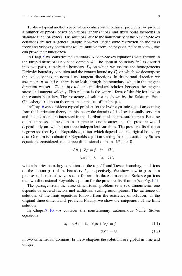
In Chap. 6 we consider a typical problem for the hydrodynamic equations comingfrom the lubrication theory. In this theory the domain of the flow is usually very thinand the engineers are interested in the distribution of the pressure therein. Becauseof the thinness of the domain, in practice one assumes that the pressure woulddepend only on two and not three independent variables. The pressure distributionis governed then by the Reynolds equation, which depends on the original boundarydata. Our aim is to obtain the Reynolds equation starting from the stationary Stokesequations, considered in the three-dimensional domains ˝", " > 0,

��u C rp D f in ˝";

div u D 0 in ˝";

with a Fourier boundary condition on the top � "F and Tresca boundary conditions

on the bottom part of the boundary �C, respectively. We show how to pass, in aprecise mathematical way, as " ! 0, from the three-dimensional Stokes equationsto a two-dimensional Reynolds equation for the pressure distribution (see Fig. 1.1).

The passage from the three-dimensional problem to a two-dimensional onedepends on several factors and additional scaling assumptions. The existence ofsolutions of the limit equations follows from the existence of solutions of theoriginal three-dimensional problem. Finally, we show the uniqueness of the limitsolution.

In Chaps. 7–10 we consider the nonstationary autonomous Navier–Stokesequations

ut � ��u C .u � r/u C rp D f ; (1.1)

div u D 0; (1.2)

in two-dimensional domains. In these chapters the solutions are global in time andunique.


Fig. 1.1 Schematic view of the problem considered in Chap. 6. Incompressible static Stokesequation is solved on the three-dimensional domain ˝". The domain thickness is given by "h,where h is a function of the point in the two-dimensional domain !. As " ! 0, Reynolds equationon ! is recovered

Chapter 7 is a general introduction to evolutionary two-dimensional Navier–Stokes equations. We prove some basic properties of solutions assuming that theexternal forces do not depend on time and that the domain of the flow is bounded.The boundary conditions are either periodic or homogeneous Dirichlet ones. In thischapter we introduce the notion of the global attractor, one of the main objects tostudy also in Chaps. 8–10.

In Chap. 8 we prove the existence of invariant measures associated with two-dimensional autonomous Navier–Stokes equations. The invariant measures aresupported on the global attractor. Then we introduce the notion of a stationarystatistical solution and prove that every invariant measure is also such a solution.Existence of the invariant measures (stationary statistical solutions) supported onthe global attractor reveals the statistical properties of the potentially chaotic fluidflow after a long time of evolution when the external forces do not depend on time.The non-autonomous case is considered in Chap. 12.

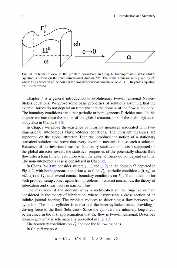
In Chaps. 9–10 we consider system (1.1) and (1.2) in the domain ˝ depicted inFig. 1.2, with homogeneous condition u D 0 on �D, periodic condition u.0; x2/ Du.L; x2/ on �L, and several contact boundary conditions on �C. The motivation forsuch problem setup comes again from problems in contact mechanics, the theory oflubrication and shear flows in narrow films.

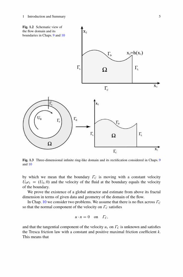
One may look at the domain ˝ as a rectification of the ring-like domainconsidered in the theory of lubrication, where it represents a cross section of aninfinite journal bearing. The problem reduces to describing a flow between twocylinders. The outer cylinder is at rest and the inner cylinder rotates providing adriving force to the fluid (lubricant). Since the cylinders are infinitely long it canbe assumed in the first approximation that the flow is two-dimensional. Describeddomain geometry is schematically presented in Fig. 1.3.

The boundary conditions on �C include the following ones.In Chap. 9 we pose

u D Ue1; U 2 R; U > 0 on �C;


Fig. 1.2 Schematic view ofthe flow domain and itsboundaries in Chaps. 9 and 10

Fig. 1.3 Three-dimensional infinite ring-like domain and its rectification considered in Chaps. 9and 10

by which we mean that the boundary �C is moving with a constant velocityU0e1 D .U0; 0/ and the velocity of the fluid at the boundary equals the velocityof the boundary.

We prove the existence of a global attractor and estimate from above its fractaldimension in terms of given data and geometry of the domain of the flow.

In Chap. 10 we consider two problems. We assume that there is no flux across �C

so that the normal component of the velocity on �C satisfies

u � n D 0 on �C;

and that the tangential component of the velocity u� on �C is unknown and satisfiesthe Tresca friction law with a constant and positive maximal friction coefficient k.This means that


jT� .u; p/j � k

jT� .u; p/j < k ) u� D U0e1

jT� .u; p/j D k ) 9� � 0 such that u� D U0e1 � �T� .u; p/

9>>>>>=

>>>>>;

on �C;

(1.3)

where T� is the tangential component of the stress tensor on �C and U0e1 D .U0; 0/,U0 2 R, is the velocity of the lower surface producing the driving force of the flow.

In the second problem the boundary �C is also assumed to be moving withthe constant velocity U0e1 D .U0; 0/ which, together with the mass force, producesthe driving force of the flow. The friction coefficient k is assumed to be related tothe slip rate through the relation k D k.ju� � U0j/, where k W RC ! R

C. If thereis no slip between the fluid and the boundary then the friction is bounded by thethreshold k.0/

u� D U0 ) jT� j � k.0/ on �C; (1.4)

while if there is a slip, then the friction force density (equal to tangential stress) isgiven by the expression

u� ¤ U0 ) �T� D k.ju� � U0j/ u� � U0

ju� � U0j on �C: (1.5)

Note that (1.4) and (1.5) generalize the Tresca law (1.3) where k was assumed tobe a constant. Here k depends of the slip rate, this dependence represents the factthat the kinetic friction is less than the static one, which holds if k is a decreasingfunction.

We prove that for both problems above there exist exponential attractors, inparticular the global attractors of finite fractal dimension.

In Chaps. 11–13 we consider the time asymptotics of solutions of the two-dimen-sional Navier–Stokes equations. First, in Chap. 11 we prove two properties of theequations in a bounded domain, concerning the existence of determining modes andnodes. Then we study the equations in an unbounded domain, in the framework ofthe theory of infinite dimensional non-autonomous dynamical systems, introducingthe notion of the pullback attractor.

Chapter 12 presents a construction of invariant measures and statistical solutionsfor the non-autonomous Navier–Stokes equations in bounded and some unboundeddomains in R

2. More precisely, we construct the family of probability measuresftgt2R and prove the relations t.E/ D �.U.t; �/�1E/ for t; � 2 R, t � � andBorel sets E in H. The support of each measure t is included in the section A.t/of the pullback attractor. We prove also the Liouville and energy equations. Finally,we consider statistical solutions of the Navier–Stokes equations supported on thepullback attractor.


In Chap. 13 we consider the problem of existence and finite dimensionality of thepullback attractor for a class of two-dimensional turbulent boundary driven flows.We generalize here the results from Chap. 9 to the non-autonomous problem. Thenew element in our study with respect to that in Chap. 9 is the allowance of thevelocity of �C to depend on time, i.e.,

u D U.t/e1; U.t/ 2 R on �C:

Our aim is to study the time asymptotics of solutions in the frame of the dynamicalsystems theory. We prove the existence of the pullback attractor and estimate itsfractal dimension. We shall apply the results from Chap. 11, reformulated here inthe language of evolutionary processes.

Chapters 14–16 are devoted to global in time solutions of the Navier–Stokesequations which are not necessary unique. We introduce theories of global attractorsfor multivalued semiflows and multivalued processes to include this situation.We study further examples of contact problems in both autonomous and non-autonomous cases.

In Chap. 14 we consider two-dimensional nonstationary Navier–Stokes shearflows in the domain ˝ as in Fig. 1.2, with nonmonotone and multivalued boundaryconditions on �C. Namely, we assume the following subdifferential boundarycondition

Qp.x; t/ 2 @j.un.x; t// on �C;

where Qp D p C 12juj2 is the Bernoulli (total) pressure, un D u � n, j W R ! R is a

given locally Lipschitz superpotential, and @j is a Clarke subdifferential of j.Our considerations are motivated here by feedback control problems for fluid

flows in domains with semipermeable walls and membranes and by the theory oflubrication. We prove the existence of global in time solutions of the consideredproblem which is governed by a partial differential inclusion, and then we provethe existence of a trajectory attractor and a weak global attractor for the associatedmultivalued semiflow.

In Chap. 15 we study the three-dimensional problem in a bounded domain ˝.The problem domain is the three-dimensional counterpart of the one presented inFig. 1.2. The boundary of ˝ is divided into three parts: the lateral one �L on whichwe assume the periodic boundary conditions, the homogeneous Dirichlet one and,finally, the contact one �C on which we consider a general form of multivaluedfrictional type boundary conditions �T� 2 g.u� /. We prove the existence of theLeray–Hopf weak solutions and, using the framework of evolutionary systems,existence of the weak global attractor.

Finally, in Chap. 16 we consider further non-autonomous and multivalued evo-lution problems, this time in the frame of the theory of pullback attractors formultivalued processes. First we prove an abstract theorem on the existence ofpullback D-attractor and then apply it to study a two-dimensional incompressible


Navier–Stokes flow with a general form of multivalued frictional contact conditionson �C. We assume that there is no flux across �C and hence we have

un.t/ D 0 on �C;

and that the tangential component of the velocity u� on �C is in the followingrelation with the tangential stresses T� ,

�T� .t/ 2 @j.x; t; u� .t// on �C:

In above formula j W �C � R � R ! R is a potential which is locally Lipschitz andnot necessarily convex with respect to the last variable, and @ is the subdifferentialin the sense of Clarke taken with respect to the last variable u� .

The tangent conditions on �C in Chaps. 15 and 16 represent the frictional contactbetween the fluid and the wall, where the friction force depends in a nonmonotoneand even discontinuous way on the slip rate, and are a generalization of theconditions considered in Chap. 10. For this case we prove the existence of theattractor.

Most chapters are devoted to two-dimensional problems. Three-dimensionalproblems are considered only in Chaps. 2, 4, 5, 6, and 15. One reason for that isassociated with the character of the Navier–Stokes equations, namely the fact thatin the two-dimensional problems it is relatively easy to prove the uniqueness of thesolutions which allows us to use the well-developed theory of infinite dimensionaldynamical systems for semigroup and processes, while the uniqueness of the three-dimensional Navier–Stokes equations is in general an open question. We alsoconsider the two- and three-dimensional problems without assuming the solutionuniqueness in the framework of (more recent) theories of trajectory attractors,multivalued semiflows, evolutionary systems, and multivalued processes.

The other reason to focus on the two-dimensional flows concern the simplicity.Our aim was to test first the more elementary two-dimensional models of somereal engineering problems. The word “test” here means not only checking the wellposedness of a particular problem. In Chap. 9 we estimate the attractor dimensionand show how it depends on the shape of the domain (cf. [24, 26], where the upperbounds of the attractor dimension depend also on the geometry of �D). Assumethat the answer to the question on the dependence of the attractor dimension on thegeometry of the boundary is such that in the two-dimensional case the estimate fromabove of the attractor dimension is independent of geometry (for example, on theroughness of the boundary represented by the oscillations of the function h D h.x1/describing �D). Such a result would be contradictory to our intuition, provided theintuitive hypotheses

attractor dimension � level of chaos in the flow � geometry of the flow domain

where “�” means “is related to,” are justified.Such a contradiction with our intuition could be resolved in the following

ways:


1. there is no such contradiction in the “real” three-dimensional case, it appearsonly in the two-dimensional case (but where lies the difference?),

2. the attractor dimension does not represent the level of chaos in the fluid flowdescribed by the (good) model of the Navier–Stokes equations,

3. the Navier–Stokes equations model is not good enough to give the right answerto the problems of chaotic movement of the classical fluids.

The close correspondence between the level of chaos in the fluid flow and thegeometry of the domain is evident as a physical phenomenon (recall observing aflow of water in the river).

To confirm the agreement of the results provided by the modeling with ourphysical intuition or else to confront the above potential possibilities motivated usto study the problems of the existence and properties of the attractor. There are stillmany interesting and important problems close to these considered in the book andwe were able to touch only a few ones. One example is to further study the relationsbetween the (type of) boundary conditions and the attractor dimension.

Finally, we remark that this book is devoted to incompressible flows, for themathematical treatise of compressible ones see, e.g., [157, 187].

2Equations of Classical Hydrodynamics

The neglected borderline between two branches of knowledge isoften that which best repays cultivation, or, to use a metaphor ofMaxwell’s, the greatest benefits may be derived from across-fertilization of the sciences.

– John William Strutt, 3rd Baron Rayleigh

In this chapter we give an overview of the equations of classical hydrodynamics.We provide their derivation, comment on the stress tensor, and thermodynamics,finally we present some elementary properties and also some exact solutions of theNavier–Stokes equations.

2.1 Derivation of the Equations of Motion

Fluid flow may be represented mathematically as a continuous transformation ofthree-dimensional Euclidean space into itself. The transformation is parametrizedby a real parameter t representing time.

Let us introduce a fixed rectangular coordinate system .x1; x2; x3/. We refer tothe coordinate triple .x1; x2; x3/ as the position and denote it by x. Now considera particle P moving with the fluid, and suppose that at time t D 0 it occupies aposition X D .X1;X2;X3/ and that at some other time t, �1 < t < C1, it hasmoved to a position x D .x1; x2; x3/. Then x is determined as a function of X and t

x D x.X; t/ or xi D xi.X; t/ : (2.1)

If X is fixed and t varies, Eq. (2.1) specifies the path of the particle initially at X.On the other hand, for fixed t, (2.1) determines a transformation of a region initiallyoccupied by the fluid into its position at time t.

© Springer International Publishing Switzerland 2016G. Łukaszewicz, P. Kalita, Navier–Stokes Equations, Advancesin Mechanics and Mathematics 34, DOI 10.1007/978-3-319-27760-8_2

11

12 2 Equations of Classical Hydrodynamics

We assume that the transformation (2.1) is continuous and invertible, that is, thereexists its inverse

X D X.x; t/; .or Xi D Xi.x; t// :

Also, to be able to differentiate, we assume that the functions xi and Xi aresufficiently smooth.

From the condition that the transformation (2.1) possess a differentiable inverseit follows that its Jacobian

J D J.X; t/ D det

�@xi

@Xj

�

satisfies

0 < J < 1 : (2.2)

The initial coordinates X of the particle will be referred to as the materialcoordinates of the particle. The spatial coordinates x may be referred to as itsposition, or place. The representation of fluid motion as a point transformationviolates the concept of the kinetic theory of fluids, as in this theory the particles aremolecules, and they are in random motion. In the theory of continuum mechanicsthe state of motion at a given point x and at a given time t is described by a numberof functions such as � D �.x; t/, u D u.x; t/, D .x; t/ representing density,velocity, temperature, and other hydrodynamical variables.

Due to the transformation (2.1), each such variable f can also be expressed interms of material coordinates

f .x; t/ D f .x.X; t/; t/ D F.X; t/ : (2.3)

The velocity u at time t of a particle initially at X is given, by definition, as

u.x; t/ D U.X; t/ D d

dtx.X; t/ ; .x D x.X; t// : (2.4)

Above, X is treated as a parameter representing a given fixed particle, and this is thereason that we use the ordinary derivative in (2.4).

Having the velocity field u.x; t/, we can (in principle) determine the transforma-tion (2.1), solving the ordinary differential equation

d

dtx.X; t/ D u.x.X; t/; t/;

with x.X; 0/ D X, where X is a parameter.We shall always write

d

dtF.X; t/ and

@

@tf .x; t/ ;

2.1 Derivation of the Equations of Motion 13

where F and f are related by (2.3). We have thus

d

dtF.X; t/ D d

dtf .x.X; t/; t/ D @f

@xi.x.X; t/; t/

dxi

dtC @f

@t.x.X; t/; t/ ;

so that by (2.4) we obtain a general formula

d

dtF.X; t/ D D

Dtf .x; t/ ; (2.5)

where DDt f .x; t/ � @f

@t .x; t/C u.x; t/ � rf .x; t/ is called the material derivative of f .

Transport Theorem Let ˝.t/ denote an arbitrary volume that is moving with thefluid and let f .x; t/ be a scalar or vector function of position and time. The transporttheorem states that

d

dt

Z

˝.t/f .x; t/ dx (2.6)

DZ

˝.t/

�@f

@t.x; t/C u.x; t/ � rf .x; t/C f .x; t/ div u.x; t/

�

dx :

For the proof consider the transformation

x W ˝.0/ ! ˝.t/; x D x.X; t/ ;

as in (2.1). Then

Z

˝.t/f .x; t/ dx

DZ

˝.0/

f .x.X; t/; t/J.X; t/ dX DZ

˝.0/

F.X; t/J.X; t/ dX ;

so that

d

dt

Z

˝.t/f .x; t/dx D d

dt

Z

˝.0/

F.X; t/J.X; t/ dX (2.7)

DZ

˝.0/

�d

dtF.X; t/J.X; t/C F.X; t/

d

dtJ.X; t/

�

dX :


By (2.5) we have

Z

˝.0/

d

dtF.X; t/J.X; t/ dX

DZ

˝.0/

�@f

@t.x.X; t/; t/C u.x.X; t/; t/ � rf .x.X; t/; t/

�

J.X; t/ dX

DZ

˝.t/

�@f

@t.x; t/C u.x; t/ � rf .x; t/

�

dx :

To prove (2.6) it remains to prove the Euler formula

d

dtJ.X; t/ D div u.x.X; t/; t/J.X; t/ ; (2.8)

the proof of which we leave to the reader as an exercise.The fluid is called incompressible if for any domain ˝.0/ and any t,

volume .˝.t// D volume .˝.0// :

From (2.7) with f .x; t/ � 1 we have

d

dtvolume .˝.t// D d

dt

Z

˝.t/dx D

Z

˝.0/

d

dtJ.X; t/dX ;

hence by (2.8), (2.2), and the arbitrariness of choice of the domain ˝.t/ via ˝.0/ anecessary and sufficient condition for the fluid to be incompressible is

div u.x; t/ D 0 :

Exercise 2.1. Prove that the transport theorem can be written in the form

d

dt

Z

˝.t/f .x; t/ dx D

Z

˝.t/

@f

@t.x; t/ dx C

Z

@˝.t/f .x; t/u.x; t/ � n.x; t/ dS ;

where n.x; t/ is the outward unit normal to @˝.t/ at x 2 @˝.t/.Equation of Continuity Let � D �.x; t/ be the mass per unit volume of a fluid atpoint x and time t. Then the mass of any finite volume ˝ is

m DZ

˝

�.x; t/ dx :


The principle of conservation of mass says that the mass of a fluid in a materialvolume ˝ does not change as ˝ moves with the fluid; that is,

d

dt

Z

˝.t/�.x; t/ dx D 0 :

From the transport theorem (2.6) it follows that

Z

˝.t/

�@�

@tC div .�u/

�

dx D 0 ;

whence

@�

@tC div .�u/ D 0 : (2.9)

Sometimes the principle of conservation of mass is expressed as follows. Let ˝ bea fixed volume. Then

d

dt

Z

˝

�.x; t/ dx D �Z

@˝

�u � n dS ; (2.10)

that is, the rate of change of mass in a fixed volume ˝ is equal to the mass fluxthrough its surface.

We notice also the general formula

d

dt

Z

˝.t/�f dx D

Z

˝.t/�

D

Dtf dx : (2.11)

Exercise 2.2. Derive (2.9) from (2.10).

Exercise 2.3 (Cf. [212]). Show that in material coordinates the equation of conti-nuity is

d

dtf�.X; t/J.X; t/g D 0 ;

or

�.X; t/J.X; t/ D �.X; 0/ :

Exercise 2.4 (Cf. [5]). Show that if �0.X/ is the distribution of density of the fluidat time t D 0 and r.div u/ D 0, then

�.x; t/ D �0.X.x; t// exp

�

�Z t

0

div u.x; t/ dt

�

:


Exercise 2.5. Find �.x; t/ for the motion

ui D xi

1C ait.a1 D 2 ; a2 D 1 ; a3 D 0/;

if �0.X/ is the distribution of density of the fluid at time t D 0.

Exercise 2.6. Prove (2.11).

Principle of Conservation of Linear Momentum We assume that the forcesacting on an element of a continuous medium are of two kinds. External, or body,forces, such as gravitation or electromagnetic forces, can be regarded as reachinginto the medium and acting throughout the volume. If f represents such a force perunit mass, then it acts on an element ˝ as

Z

˝

�f dx :

The internal, or contact, forces are to be regarded as acting on an element of volume˝ through its bounding surface. Let n be the unit outward normal at a point ofthe surface @˝, and tn the force per unit area exerted there by the material volumeoutside @˝. Then the surface force exerted on the volume ˝ can be expressed bythe integral

Z

@˝

tn dS :

The Cauchy principle says that tn depends at any given time only on the positionand the orientation of the surface element dS; in other words,

tn D tn.x; t; n/ :

The principle of conservation of linear momentum says that the rate of change oflinear momentum of a material volume equals the resultant force on the volume

d

dt

Z

˝.t/�udx D

Z

˝.t/�f dx C

Z

@˝.t/tn dS ; (2.12)

where f is assumed to be known.By (2.11), (2.12) yields

Z

˝.t/�

Du

Dtdx D

Z

˝.t/�f dx C

Z

@˝.t/tn dS : (2.13)

From this equation we derive a very important fact, namely, that the vector tn (callednormal stress) can be expressed as a linear function of n, in the form

tn.x; t; n/ D n.x; t/T.x; t/ ; (2.14)


where T D fTijg is a matrix called the stress tensor. This will allow us to pass fromthe integral form (2.13) of the equation of conservation of linear momentum to adifferential one.

Let l3 be the volume of˝ D ˝.t/. Dividing both sides of (2.13) by l2 and lettingthe volume tend to zero we obtain

limj˝j!0

l�2Z

@˝

tn dS D 0 ; (2.15)

that is, the stress forces are in local equilibrium.Let ˝ be a domain containing a fluid, and consider a regular tetrahedron with

vertex at an arbitrary point x 2 @˝, and with three of its faces parallel to thecoordinate planes. Let the slanted face have normal n D .n1; n2; n3/ and area ˙ .The normals to the other faces are �e1, �e2, and �e3, and their areas are n1˙ , n2˙ ,and n3˙ . Applying (2.15) to the family of tetrahedrons obtained by letting ˙ ! 0,we obtain

t.n/C n1t.�e1/C n2t.�e2/C n3t.�e3/ D 0 ; (2.16)

where t.n/ D tn D tn.x; t; n/, t.�h/ D t�h for h 2 fe1; e2; e3g, and ni > 0. Bya continuity argument, (2.16) holds for all ni � 0, and then we prove easily thatt.ei/ D �t.�ei/, i D 1; 2; 3, and that it holds for all n. This means that t.n/ may beexpressed as a linear function of n; that is, we can write it in the form (2.14). Thus,by (2.13) and by the Green theorem we obtain

Z

˝.t/�

Du

Dtdx D

Z

˝.t/.�f C div T/ dx ;

whence, by the arbitrariness of the domain of integration,

�Du

DtD �f C div T ; (2.17)

or

�

0

@@

@tui C

3X

jD1uj@

@xjui

1

A D �fi C Tji;j; i D 1; 2; 3 :

This is the general Cauchy equation of motion in differential form.

Exercise 2.7. Give a physical interpretation of the components of the stress tensor.

Notice that we have not specified T yet, that is, we have not made anyassumptions concerning the nature of forces acting on surface elements. Theseforces depend on the kind of fluid, or, more generally, on the kind of medium underconsideration.


In the simplest model the contact forces act perpendicularly to the surfaceelements. We have then

t.n/ D �p.x/n ;

and call p the pressure. The minus sign is chosen so that when p > 0, the contactforces on a closed surface tend to compress the fluid inside; p represents the pressureexerted from outside on a surface of the element of the fluid.

In particular, all fluids at rest exhibit this stress behavior, namely that an elementof area always experiences a stress normal to itself, and this stress is independent ofthe orientation. Such stress is called hydrostatic.

We call this idealized model a perfect fluid. The equation of motion for perfectfluids is

�

�@u

@tC .u � r/u

�

D �f � rp ;

where

.u � r/ui D3X

jD1uj@

@xjui ; i D 1; 2; 3 :

All real fluids when in motion can exert tangential stresses across surface elements,in which case the tensor T is not diagonal.

The stress tensor may always be written in the form

Tij D �pıij C Pij :

In this case Pij is called the viscous stress tensor.In classical fluid dynamics it is assumed that the stress tensor is symmetric, that is,

Tij D Tji :

This assumption has very important consequences. It may be also considered as atheorem if we assume a specific form of the equation of conservation of angularmomentum. We shall discuss this in Sect. 2.2.

Exercise 2.8 (Cf. [5]). Show that the Cauchy equation of motion can be written as

@

@t.�ui/ D �fi C .Tji � �ujui/;j ;

and interpret it physically.


Exercise 2.9 (Cf. [5]). Show that if F is any function of position and time, thenZ

@˝

FTjinj dS DZ

˝

�

TjiF ;j C�F

�Dui

Dt� fi

��

dx

(theorem of stress means).

Equation of Energy The first law of thermodynamics in classical hydrodynamicsstates that the increase of total energy (we shall consider here only kinetic andinternal energies) in a material volume is the sum of the heat transferred and thework done on the volume. We denote by q the heat flux (then �q � n is the heat fluxinto the volume) and by E the specific internal energy. Then the balance expressedby the first law of thermodynamics is, cf. [5],

d

dt

Z

˝.t/�

�1

2juj2 C E

�

dx (2.18)

DZ

˝.t/�f � u dx C

Z

@˝.t/tn � u dS �

Z

@˝.t/q � n dS :

The first integral on the right-hand side is the rate at which the body force does work,the second integral represents the work done by the stress, and the third integralis the total heat flux into the volume.

We shall write this equation in another form. From the theorem of stress means(Exercise 2.9) we have, with F D ui,

Z

@˝.t/uiTjinj dS D

Z

˝.t/

�

Tjiui;j C �uiDui

Dt� �fiui

�

dx :

Rearranging the terms and using the transport theorem, we obtain

d

dt

Z

˝.t/�1

2juj2 dx D

Z

˝.t/�1

2

D

Dtjuj2 dx (2.19)

DZ

˝.t/�fiui dx �

Z

˝.t/Tjiui;j dx C

Z

@˝.t/ui.tn/i dS :

Thus the rate of change of kinetic energy of a material volume is the sum of threeparts: the rate at which the body forces do work, the rate at which the internalstresses do work, and the rate at which the surface stresses do work.

From (2.18), (2.19), the transport theorem, and the Green theorem we obtain

Z

˝.t/

�

�DE

DtC r � q � T W .ru/

�

dx D 0 ;

where T W .ru/ is the dyadic notation for Tjiui;j, the scalar product of T and ru.


Thus

�DE

DtD �r � q C T W .ru/ :

Conservation Laws of Classical Hydrodynamics Above we obtained the follow-ing system of conservation laws of classical hydrodynamics

D�

DtD ��r � u ; (2.20)

�Du

DtD r � T C �f ; (2.21)

�DE

DtD �r � q C T W .ru/ : (2.22)

They are laws of conservation of mass, momentum, and energy, respectively.If we assume the Fourier law for the conduction of heat,

q D �kr .k � 0/ ; (2.23)

where k is the thermal conductivity of the fluid then the energy equation takes theform

�DE

DtD r � .kr/C T W .ru/ :

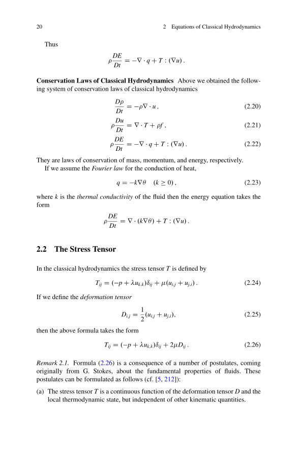
2.2 The Stress Tensor

In the classical hydrodynamics the stress tensor T is defined by

Tij D .�p C �uk;k/ıij C .ui;j C uj;i/ : (2.24)

If we define the deformation tensor

Di;j D 1

2.ui;j C uj;i/; (2.25)

then the above formula takes the form

Tij D .�p C �uk;k/ıij C 2Dij : (2.26)

Remark 2.1. Formula (2.26) is a consequence of a number of postulates, comingoriginally from G. Stokes, about the fundamental properties of fluids. Thesepostulates can be formulated as follows (cf. [5, 212]):

(a) The stress tensor T is a continuous function of the deformation tensor D and thelocal thermodynamic state, but independent of other kinematic quantities.

2.2 The Stress Tensor 21

(b) The fluid is homogeneous; that is, T does not depend explicitly on x.(c) The fluid is isotropic; that is, there is no preferred direction.(d) When there is no deformation (D D 0), and the fluid is incompressible

(uk;k D 0), the stress is hydrostatic (T D �pI, I is the unit matrix).

Fluids that satisfy these postulates are called Stokesian. It can be proved (cf. [5, 212])that the most general form of the stress tensor in this case is

T D .�p C ˛/I C ˇD C �D2 ;

where p; ˛; ˇ; � are some functions that depend on the thermodynamic state, ˛; ˇ; �being dependent as well on the invariants of the tensor D.

Moreover, when the dependence of the components of T on the components ofD is postulated to be linear, the stress tensor can be written as

T D .�p C � div u/I C 2D ;

which coincides with (2.24). Such linear Stokesian fluids are called Newtonian.Fluids that are not Newtonian are called non-Newtonian. One important exampleof the latter are the micropolar fluids [92, 159].

The Stress Tensor and the Law of Conservation of Angular MomentumLooking at the form of the equation of conservation of linear momentum

d

dt

Z

˝.t/�u dx D

Z

˝.t/�f dx C

Z

@˝.t/tn dS ;

and recalling the definition of angular momentum in mechanics of mass pointsor rigid particles, it seems natural to assume the following form of the law ofconservation of angular momentum:

d

dt

Z

˝.t/�.x � u/ dx D

Z

˝.t/�.x � f / dx C

Z

@˝.t/x � tn dS : (2.27)

In fact, this form of the law of conservation of angular momentum holds if weassume that all torques arise from macroscopic forces. This is the case in mostcommon fluids, but a fluid with a strongly polar character, e.g., a polyatomic fluid,is capable of transmitting stress torques and being subjected to body torques. Wecall such fluids polar.

Theorem 2.1. For an arbitrary continuous medium satisfying the continuityequation (2.9) and the dynamical equation (2.17) the following statements areequivalent:

(i) the stress tensor is symmetric,(ii) equation (2.27) holds.


Remark 2.2. In classical hydrodynamics the stress tensor is symmetric, and the lawof conservation of angular momentum is defined by Eq. (2.27). In consequence,in classical hydrodynamics the law of conservation of angular momentum can bederived from the law of conservation of mass and the law of conservation of linearmomentum, and as such adds nothing to the description of the fluid.

Proof. Let us assume (ii), and we shall deduce (i). Applying formula (2.11), wehave from (2.27)

d

dt

Z

˝.t/�.x � u/ dx (2.28)

DZ

˝.t/�

D

Dt.x � u/ dx D

Z

˝.t/�

�

x � Du

Dt

�

dx

DZ

˝.t/�.x � f / dx C

Z

@˝.t/x � tn dS :

By the Green theorem,Z

@˝.t/x � tn dS D

Z

˝.t/.x � .r � T/C Tx/ dx ; (2.29)

where r � T is another notation for div T , and Tx is the vector �ijkTjk (�ijk is thealternating tensor of Levi-Civita), so that by (2.28)

Z

˝.t/x �

�

�Du

Dt� �f � r � T

�

dx DZ

˝.t/Tx dx :

The left-hand side vanishes identically by the Cauchy equation; hence the right-handside vanishes for an arbitrary volume, and so Tx D 0. However, the components ofTx are T23 � T32, T31 � T13, T12 � T21, and the vanishing of these implies Tij D Tji,so that T is symmetric.

We leave to the reader the proof that (i) implies (ii). ut

2.3 Field Equations

Substituting the stress tensor (2.24) into the system (2.20)–(2.22) we obtain thesystem of field equations of classical hydrodynamics

D�

DtD ��r � u ; (2.30)

�Du

DtD �rp C .�C /r div u C �u C �f ; (2.31)

2.4 Navier–Stokes Equations 23

�DE

DtD �p div u C �˚ � r � q ; (2.32)

where

�˚ D �.div u/2 C 2D W D (2.33)

is the dissipation function of mechanical energy per mass unit.Let us assume that the fluid is viscous and incompressible, namely, that > 0

and

div u D 0 ; (2.34)

that the specific internal energy of the fluid is proportional to its temperature,

E D cr ; where cr D const > 0 ; (2.35)

and that Fourier’s law (2.23) (with k D const � 0) holds. With (2.34), (2.35), (2.23),and (2.33), system (2.30)–(2.32) becomes

@�

@tC u � r� D 0 ; div u D 0 ; (2.36)

�

�@u

@tC .u � r/u

�

D �rp C �u C �f ; (2.37)

�cr

�@

@tC u � r

�

D 2D W D C k�: (2.38)

2.4 Navier–Stokes Equations

Assuming that the density � of the fluid is uniform and denoting � D

�, D k

�(�

is called the kinematic viscosity coefficient), Eqs. (2.36)–(2.38) reduce to

@u

@tC .u � r/u D �1

�rp C ��u C f ; (2.39)

div u D 0 ; (2.40)

cr

�@

@tC u � r

�

D 2�D W D C �: (2.41)


When the body forces f do not depend on temperature, the first two equations of theabove system,

@u

@tC .u � r/u D �1

�rp C ��u C f ; (2.42)

div u D 0 (2.43)

constitute a closed system of equations with respect to variables u; p, and are calledNavier–Stokes equations of viscous incompressible fluids with uniform density (weshall call them just the Navier–Stokes equations). The mechanical energy of the flowgoverned by (2.42) and (2.43) due to viscous dissipation is lost and appears as heat.This can be seen from Eq. (2.41) in which the term 2�D W D is positive, providedthe flow is not uniform. In real fluids, however, density depends on temperature,so that our system (2.39)–(2.41) may be physically impossible. In fact, due toviscosity and high velocity gradients the temperature rises in view of (2.41), and thisproduces density fluctuations, contrary to our assumption that density is uniform inthe flow domain. Thus, reduced problems often play the role of more or less justifiedapproximations. For more considerations of this kind cf. [109, Chap. 1].

When the body forces depend on temperature, f D f ./, we have to take intoaccount the whole system (2.39)–(2.41). One of the considered in the literaturesystem of equations of heat conducting viscous and incompressible fluid are theso-called Boussinesq equations,

@u

@tC .u � r/u D � 1

�0rp C ��u C 1

�0g˛. � 0/ ; (2.44)

div u D 0 ; (2.45)

@

@tC u � r D

cr� ; (2.46)

where g represents the vertical gravity acceleration, ˛ is the thermal expansioncoefficient, and

cris the thermal diffusion coefficient. Moreover, �0 and 0 are

some reference density and temperature, respectively. In the velocity equation thevertical buoyancy force 1

�0g˛. � 0/ results from changes of density associated

with temperature variations � � �0 D �˛. � 0/. This is the only term in thesystem where changes of density were taken into account. We have also abandonedthe viscous dissipation term in the temperature equation.

2.5 Vorticity Dynamics

Taking the curl of the equation of motion

@u

@tC .u � r/u D �1

�rp C ��u;

2.5 Vorticity Dynamics 25

we obtain

@!

@tC .u � r/! D .! � r/u C ��!; (2.47)

where the vector field ! D r � u is called vorticity of the fluid. It has a simplephysical interpretation. In the case of two-dimensional motion with

u D .u1.x; y/; u2.x; y/; 0/;

the vorticity reduces to

! D .0; 0; !3.x1; x2// D�

0; 0;@u2.x1; x2/

@x1� @u1.x1; x2/

@x2

�

;

where the third component represents twice the angular velocity of a small(infinitesimal) fluid element at point .x1; x2/. The vorticity field is, by definition,divergence free,

div! D 0:

In the case of two-dimensional motions the Eq. (2.47) reduces to

@!

@tC .u � r/! D ��!;

and we can see that the vorticity in the fluid is transported by two agents: convectionand diffusion, just as the temperature in the system (2.44)–(2.46).

For inviscid fluids (� D 0) the vorticity field has very important properties thatallow us to imagine behavior of complicated turbulent flows [83]. In this case,vorticity is a local variable which means that we can isolate a patch of vorticity andobserve how it is transported along the velocity field trajectories with a finite speed.For two-dimensional flows this is evident as then the vorticity equation reduces to

@!

@tC .u � r/! D 0:

For more information, cf. [166].

Exercise 2.10. Vorticity has nothing in common with rotation of the fluid as awhole. Calculate the vorticity of the flows: (a) u.x1; x2; x3/ D .u1.x2/; 0; 0/ and(b) u.r; �; z/ D .0; k=r; 0/ for r > 0.


2.6 Thermodynamics

Equations of State From the point of view of thermodynamics the state of ahomogeneous fluid can be described by some definite relations among a numberof certain state variables, the most important being the volume V .V D 1=�/, theentropy S, the internal energy E, the pressure p, and the absolute temperature ,cf. [212].

In such a description one may start with a relation of the form (cf. [212])

E D E.S;V/ (Gibbs relation) (2.48)

and define p and by

p D �@E

@V; D @E

@S; (2.49)

with p; > 0 by assumption. In this case, taking the total differential in (2.48) andusing (2.49), we obtain

dE D dS � p dV or dE D dS � p1

�2d� : (2.50)

A simple phase system is said to undergo a differentiable process if its state variablesare differentiable functions of time: V D V.t/, S D S.t/, etc. Assuming such adependence one usually assumes, together with (2.50), that

DE

DtD

DS

Dt� p

DV

Dt

or

DE

DtD

DS

Dt� p

1

�2D�

Dt: (2.51)

Relation (2.51) makes it possible to write a definite form of the balance of entropywhen we know the laws of conservation of mass and internal energy. We shall usethis relation in the sequel.

Second Law of Thermodynamics and Constraints on Viscosity CoefficientsConsider the law of conservation of energy (2.32)

�DE

DtD r � .kr/ � p div u C �˚ ; (2.52)

where Fourier’s law is assumed, and �˚ is given by (2.33). We see that the internalenergy increases with the influx of heat transfer, compression, and the viscousdissipation.

Documents

Grzegorz Łukaszewicz Piotr Kalita Navier– Stokes Equations