Embed Size (px)
Citation preview

Handling Count Data in Clinical Trials
Mani Lakshminarayanan, Ph.D.Pfizer, Inc
Biostatistics Day, Rutgers University
February 16, 2007Based on joint research with Madhuja Mallick (Merck), Aparna Raychaudhuri (Centocor) and Simon Davies (Pfizer)

What happens if you have too many zeros?

OUTLINE
• Issues in Early Phase Trials• Count data as an Endpoint• Poisson Distribution• Dose Response• Introduction to GLM• Over-dispersion in Counts
– Negative Binomial– Zero-inflated Poisson
• Examples• Simulation Results• Sample Size• Conclusion

Issues in Early Phase Clinical Trials
• Define and explore endpoints• Dose selection• Early indication of efficacy and safety• PK/PD
The first two topics, definition of endpoints and dose selection, are discussed here.
Count Data as an Endpoint
• Examples– Number of new enhancing lesions seen
on monthly MRI of the brain– Number of hospitalizations over a period
of time– Blood cells in a blood sample
(space=volume)– Number of patients “at risk” with a differing
years of exposure

2003, Vol 348, p 15-23


Count data can be modeled using Poisson distribution
Poisson Properties
• Poisson distribution for the Count Data can be used if– The expected number of events occurring
in an interval of time is proportional to the size of the interval
– The probability that two events occurring in an infinitesimally small interval of space-time is 0
– The number of events occurring in separate intervals of space-time are independent
Properties (contd)
• For a Poisson random variable with parameter λ, E(Y)=Var(Y) = λ
• Since mean equals the variance, any factor that affects one will also affect the other– Usual assumption of homoscedasticity is not
appropriate for Poisson data• Poisson distribution provides an
approximation to the binomial for rare events, where p is small and n is large
• Sum of independent Poisson is also a Poisson
Properties (contd)
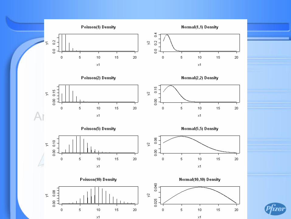
• Normal approximation is satisfactory for λ>5 and the proportion λ/n is not too close to zero or one– Transformations (logarithmic or arcsine square
root) may also be used• Excessive zero counts may make the
variance > mean, overdispersion– Failure to observe an event during the period– Inability ever to experience an event

Model Details

Generalized Linear Model (GLM)
• Definition– A vector of observations y of length N is assumed
to be a realization of a vector of iid random variables Y with mean µ. A set of covariates x1, x2,……,xp defines a linear predictor:
η = Σ βj xj
• The classical linear model can be written in a tripartite form:
Classical Linear Model
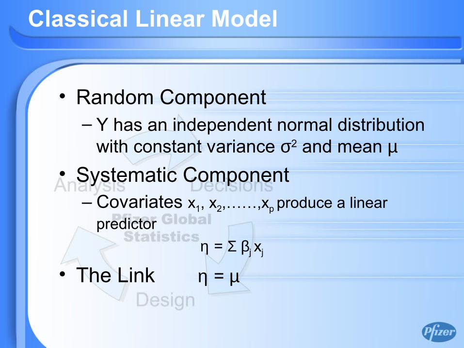
• Random Component– Y has an independent normal distribution
with constant variance σ2 and mean µ• Systematic Component
– Covariates x1, x2,……,xp produce a linear predictor
η = Σ βj xj
• The Link η = µ
Generalized Linear Model
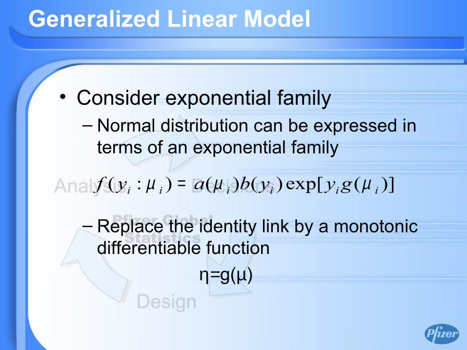
• Consider exponential family– Normal distribution can be expressed in
terms of an exponential family
– Replace the identity link by a monotonic differentiable function
η=g(µ)
)](exp[)()():( iiiiii gyybayf µµµ =
Exponential family
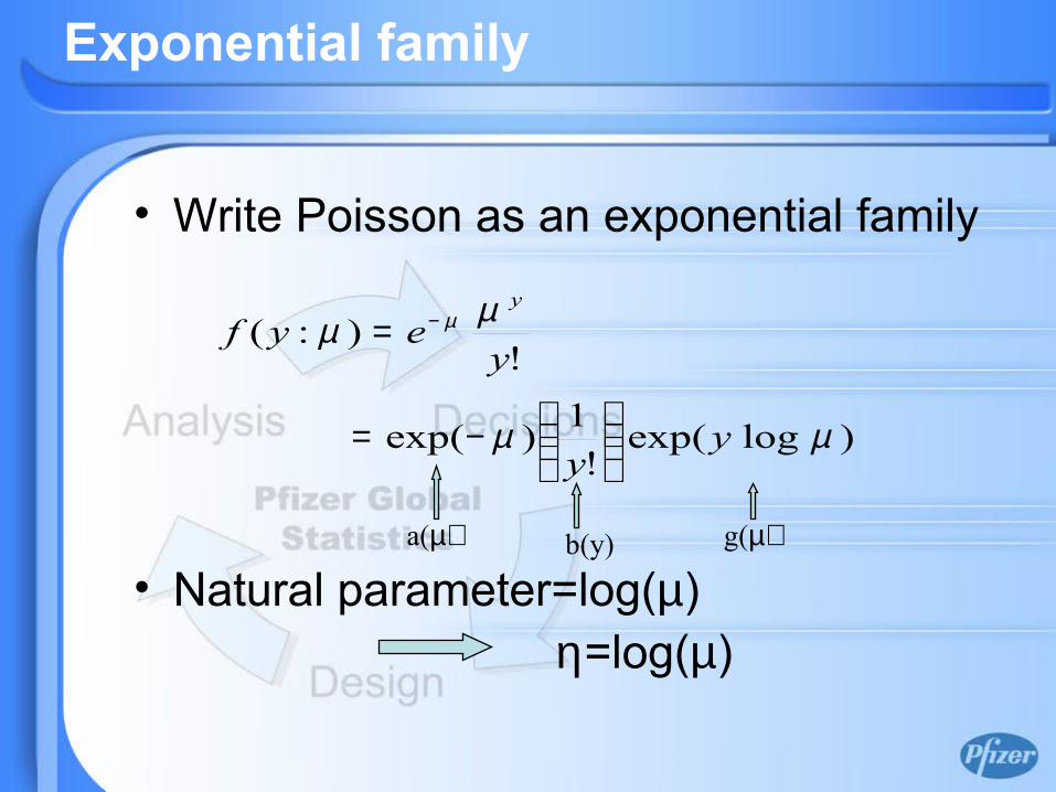
• Write Poisson as an exponential family
• Natural parameter=log(µ)η=log(µ)
)logexp(!
1)exp(
!):(
µµ
µµ µ
yy
yeyf
y
−=
= −
a(µ) b(y) g(µ)

Poisson Models
• Link Functionln µi = η = xi
Tβ
– Log link ensures– Poisson model with log link is sometimes
called log-linear model– Also, this is the canonical link
),0[~ ∞∈µ
Fitting the Model
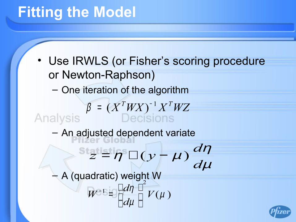
• Use IRWLS (or Fisher’s scoring procedure or Newton-Raphson)– One iteration of the algorithm
– An adjusted dependent variate
– A (quadratic) weight W
WZXWXX TT 1)( −=β
µηµη
ddyz )( −+=
)(2
1 µµη V
ddW
=−
Fitting the Model
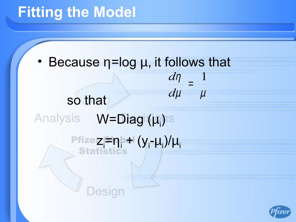
• Because η=log µ, it follows that
so thatW=Diag (µi)zi=ηi + (yi-µi)/µi
µµη 1=
dd
Fitting the Model
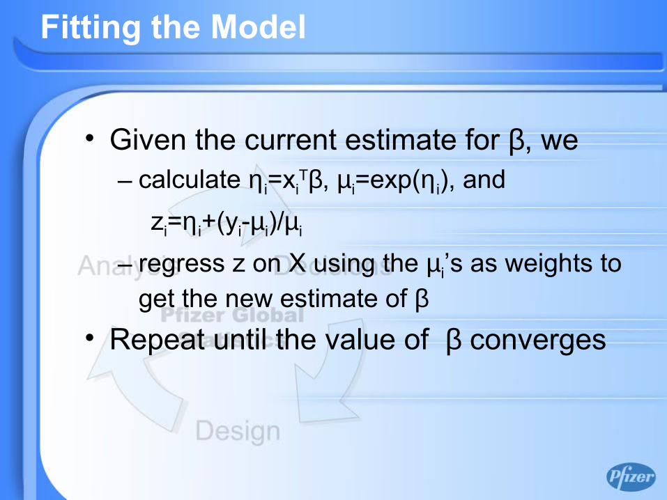
• Given the current estimate for β, we– calculate ηi=xi
Tβ, µi=exp(ηi), and zi=ηi+(yi-µi)/µi
– regress z on X using the µi’s as weights to get the new estimate of β
• Repeat until the value of β converges

Over-dispersion
A Simple Test for Over-dispersion
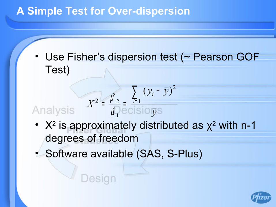
• Use Fisher’s dispersion test (~ Pearson GOF Test)
• X2 is approximately distributed as χ2 with n-1 degrees of freedom
• Software available (SAS, S-Plus)
y
yyX i
i∑=
−== 1
2
1
22)(
ˆˆ
µµ
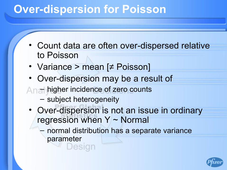
Over-dispersion for Poisson
• Count data are often over-dispersed relative to Poisson
• Variance > mean [≠ Poisson]• Over-dispersion may be a result of
– higher incidence of zero counts– subject heterogeneity
• Over-dispersion is not an issue in ordinary regression when Y ~ Normal– normal distribution has a separate variance
parameter
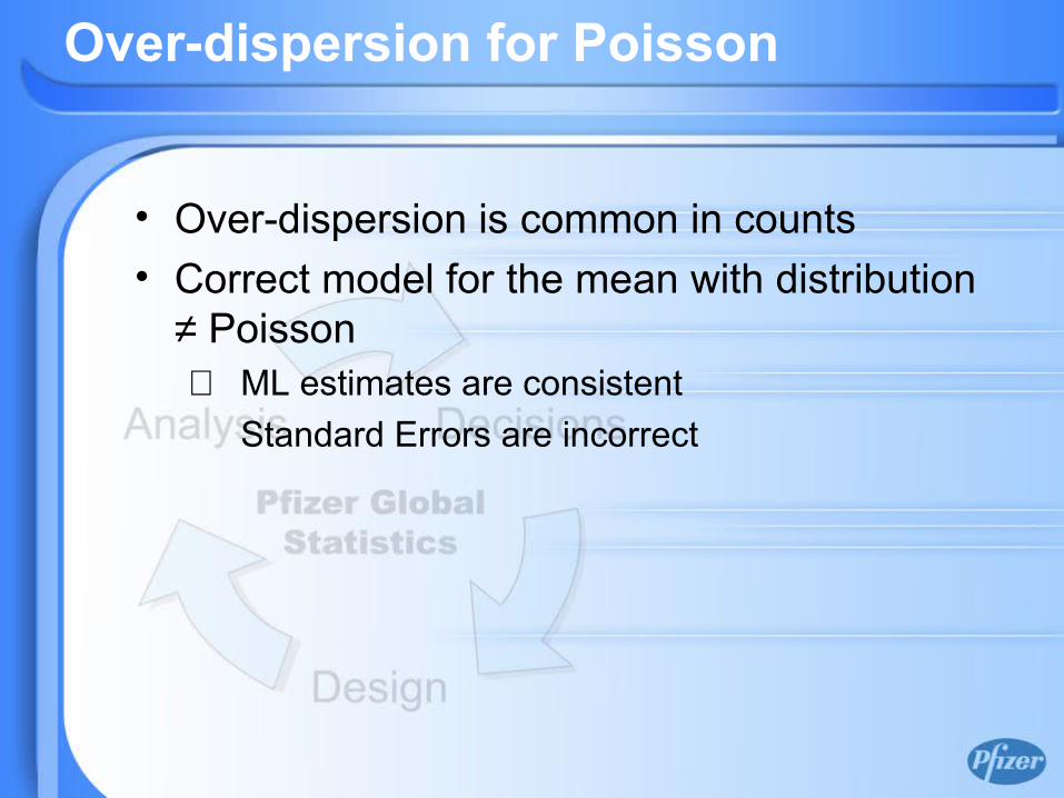
Over-dispersion for Poisson
• Over-dispersion is common in counts• Correct model for the mean with distribution
≠ Poisson⇒ ML estimates are consistent
Standard Errors are incorrect
Models for Over-dispersion
• Negative Binomial• Zero-inflated Poisson• Others..
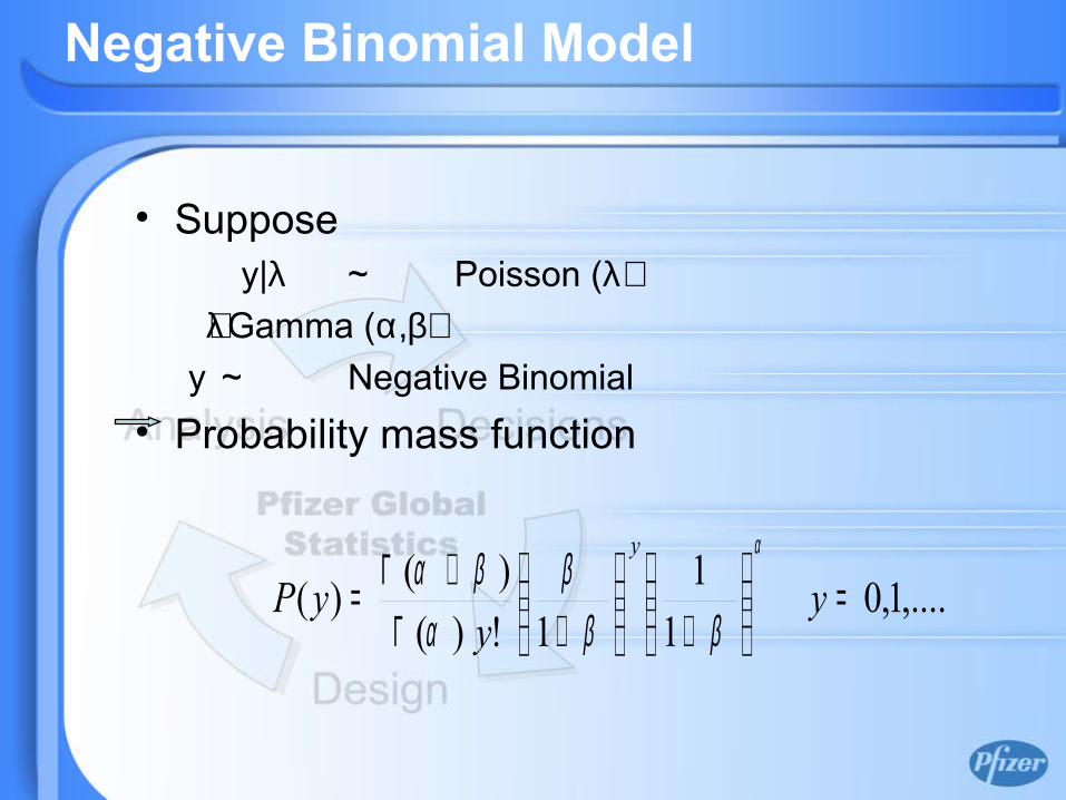
Negative Binomial Model
• Supposey|λ ~ Poisson (λ)
λ∼Gamma (α,β)y ~ Negative Binomial
• Probability mass function
,....1,01
11!)(
)()( =
+
+Γ
+Γ= yy
yPy α
βββ
αβα
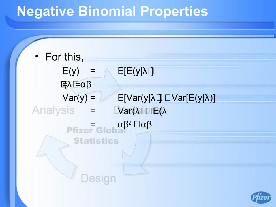
Negative Binomial Properties
• For this,E(y) = E[E(y|λ)]
= Ε(λ)=αβVar(y) = E[Var(y|λ)] + Var[E(y|λ)]
= Var(λ) + E(λ)= αβ2 + αβ
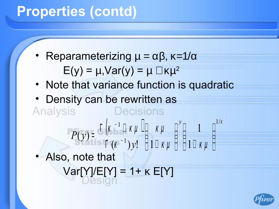
Properties (contd)
• Reparameterizing µ = αβ, κ=1/αE(y) = µ,Var(y) = µ + κµ2
• Note that variance function is quadratic• Density can be rewritten as
• Also, note thatVar[Y]/E[Y] = 1+ κ E[Y]
( ) κ
κ µκ µκ µ
κκ µκ
/1
1
1
11
1!)()(
+
+Γ
+Γ= −
− y
yyP
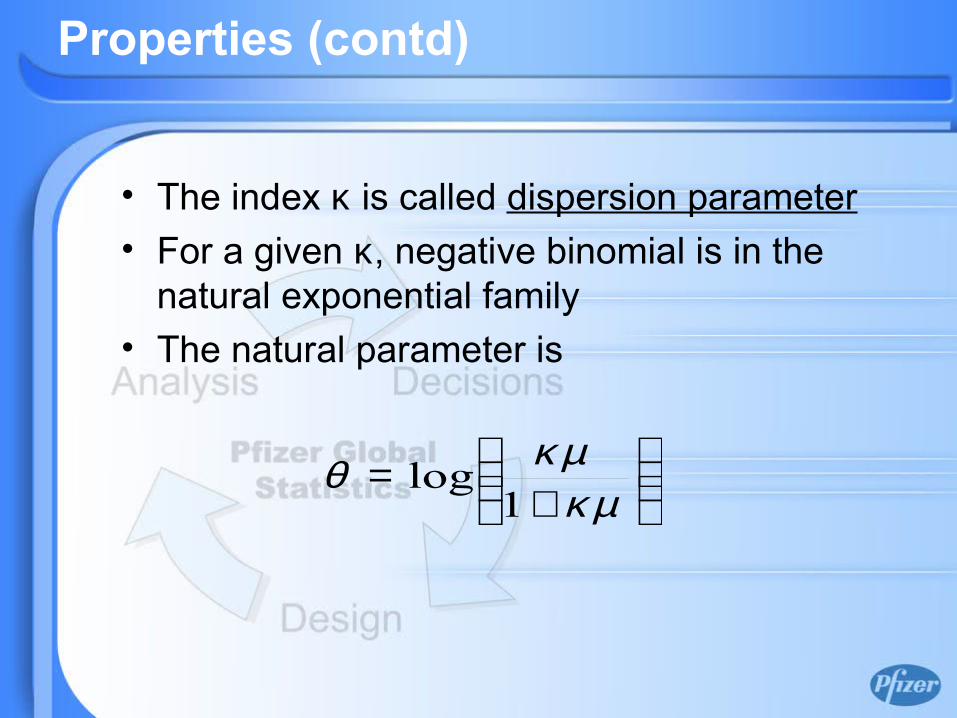
Properties (contd)
• The index κ is called dispersion parameter• For a given κ, negative binomial is in the
natural exponential family• The natural parameter is
+
=κµ
κµθ1
log

Remarks
• The greater κ, the greater the over-dispersion compared to the ordinary Poisson GLM
• If κ were known, we could fit the model by IRWLS to obtain the MLE of β
• Estimating κ is problematic, need to jointly estimate κ and β

When there are excessive zeros?
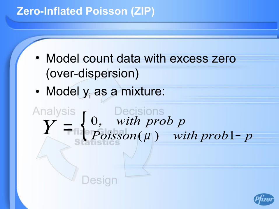
Zero-Inflated Poisson (ZIP)
• Model count data with excess zero (over-dispersion)
• Model yi as a mixture:
{ pprobwithpprobwithPoissonY ,0
1)( −= µ
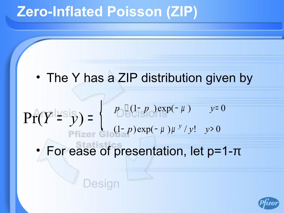
Zero-Inflated Poisson (ZIP)
• The Y has a ZIP distribution given by
• For ease of presentation, let p=1-π
{ 0)exp()1(
0!/)exp()1()Pr(
=−−+
>−−==
ypp
yyp yyY
µ
µµ
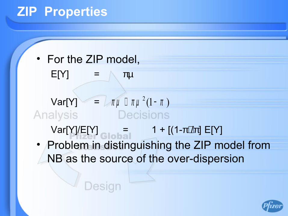
ZIP Properties
• For the ZIP model,E[Y] = πµ
Var[Y] =
Var[Y]/E[Y] = 1 + [(1-π)/π] E[Y]• Problem in distinguishing the ZIP model from
NB as the source of the over-dispersion
)1(2 ππ µπ µ −+
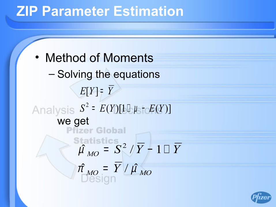
ZIP Parameter Estimation
• Method of Moments– Solving the equations
we get)](1)[(
][2 YEYES
YYE−+=
=
µ
MOMO
MO
YYYS
µπµ
ˆ/ˆ1/ˆ 2
=+−=
ZIP Parameter Estimation
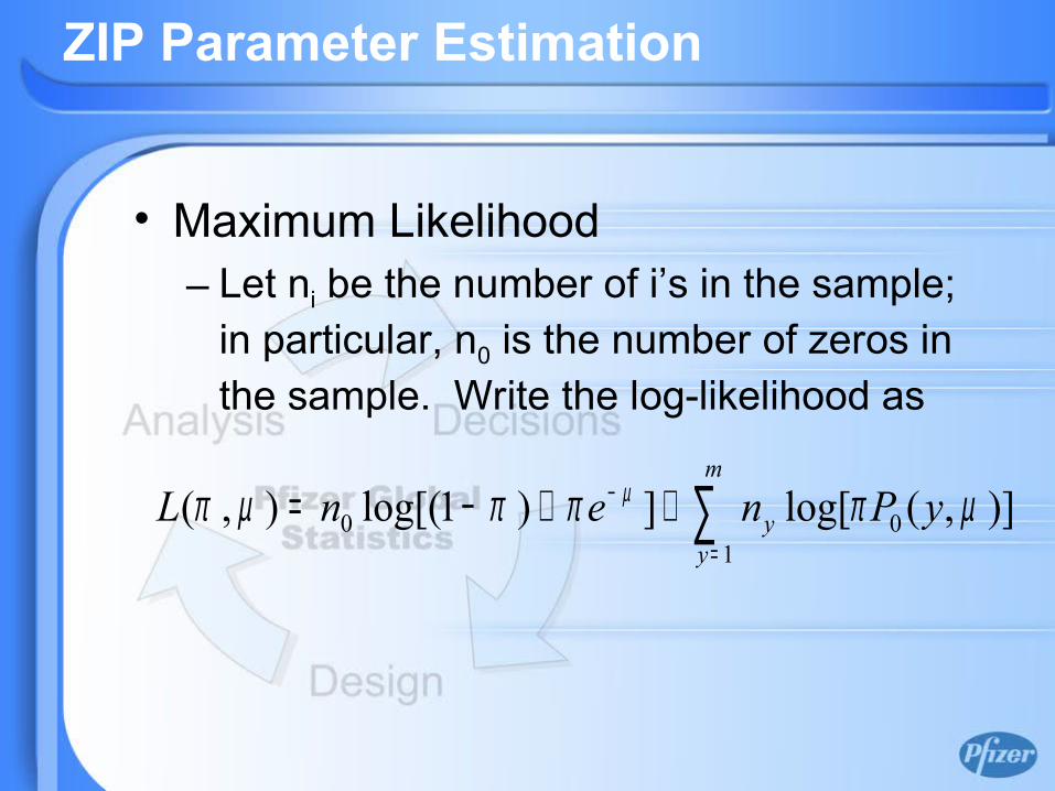
• Maximum Likelihood– Let ni be the number of i’s in the sample;
in particular, n0 is the number of zeros in the sample. Write the log-likelihood as
)],(log[])1log[(),(1
00 µπππµπ µ yPnenLm
yy∑
=
− ++−=
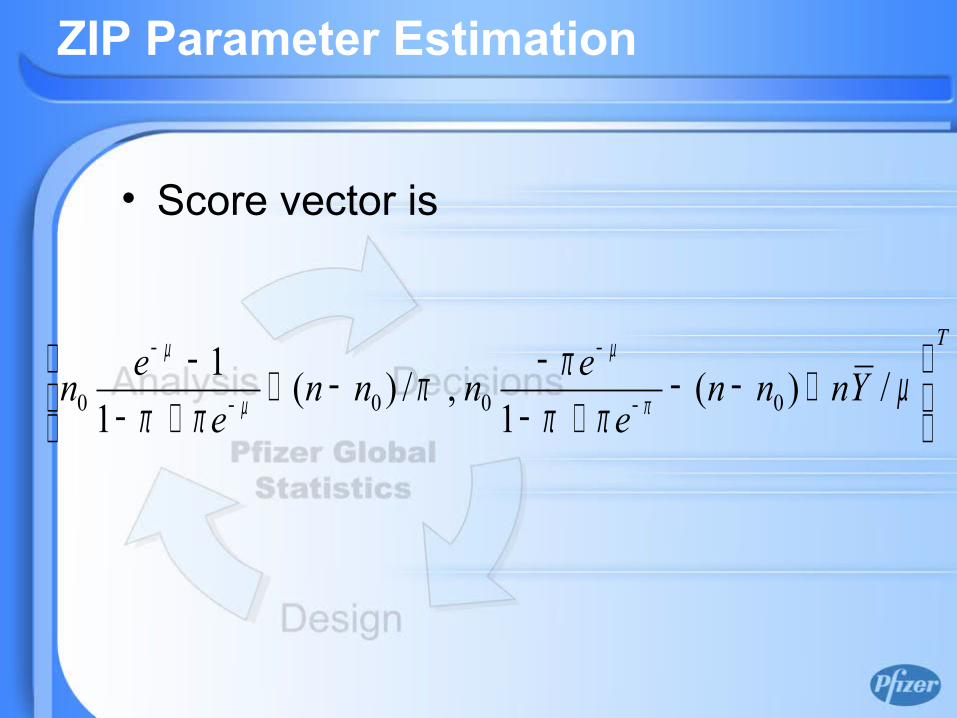
ZIP Parameter Estimation
• Score vector is
T
Ynnne
ennne
en
+−−
+−−−+
+−−
−
−
−
−
µππ
ππππ π
µ
µ
µ
/)(1
,/)(1
10000
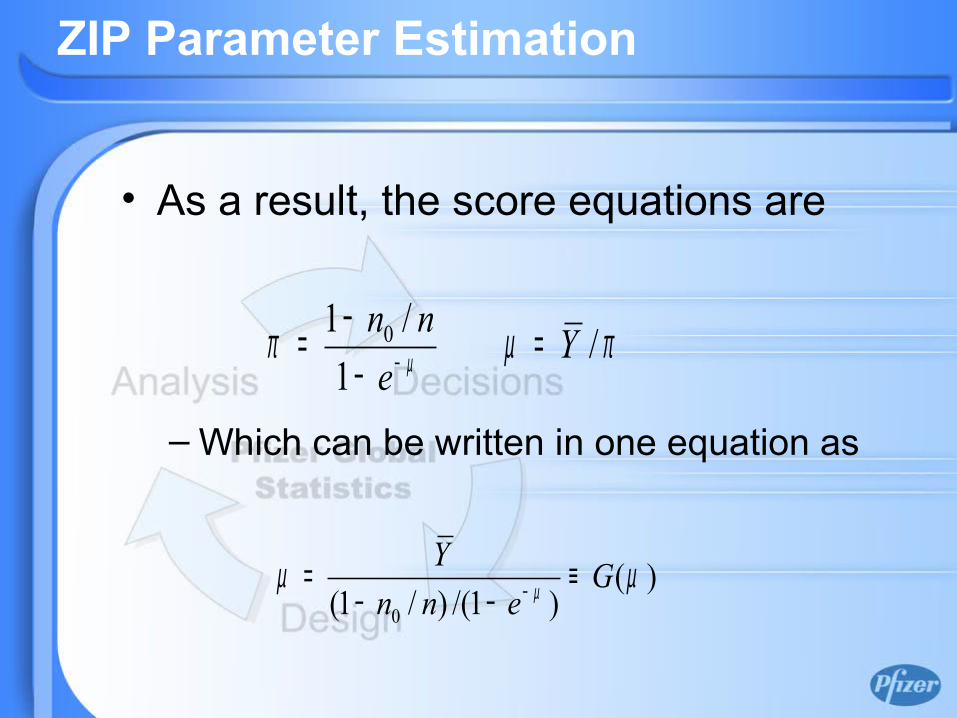
ZIP Parameter Estimation
• As a result, the score equations are
– Which can be written in one equation as
πµπ µ /1
/1 0 Ye
nn =−
−= −
)()1/()/1( 0
µµ µ Genn
Y ≡−−
= −
Estimation
• Need iteration to solve this equation• Since G'(µ) > 0, µj+1 = G(µj) converges
for any initial value µ0 to the MLE satisfying the equation µ=G(µ).
• Choose the moment estimate as the initial value
• Can use EM Algorithm

Example

Seizure Counts in Epileptics
Seizure counts in Epileptics
• Thall, P. F. and Vail, S. C. (1990) Some covariance models for longitudinal count data with over-dispersion. Biometrics 46, 657–671
• Data set on two-week seizure counts for 59 epileptics. The number of seizures was recorded for a baseline period of 8 weeks, and then patients were randomly assigned to a treatment group or a control group. Counts were then recorded for four successive two-week periods (response: count for the 2 week period, 236 observed counts). The subject's age is the only covariate.
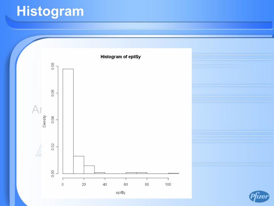
Histogram
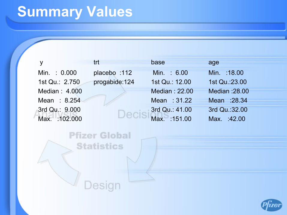
Summary Values
y trt base age Min. : 0.000 placebo :112 Min. : 6.00 Min. :18.00 1st Qu.: 2.750 progabide:124 1st Qu.: 12.00 1st Qu.:23.00 Median : 4.000 Median : 22.00 Median :28.00 Mean : 8.254 Mean : 31.22 Mean :28.34 3rd Qu.: 9.000 3rd Qu.: 41.00 3rd Qu.:32.00 Max. :102.000 Max. :151.00 Max. :42.00

Number of Tumors

Example
• Development of mammary cancer in rats• Ref: M.H. Gail et al, Biometrics, June 1980• Animals injected with carcinogen and given
retinyl acetate to prevent cancer for 2 months
• Those that remain cancer-free were randomized to retinoid prophylaxis (treatment, 23 rats) or control (25 rats)
• Number of tumors developed over 4 months were reported

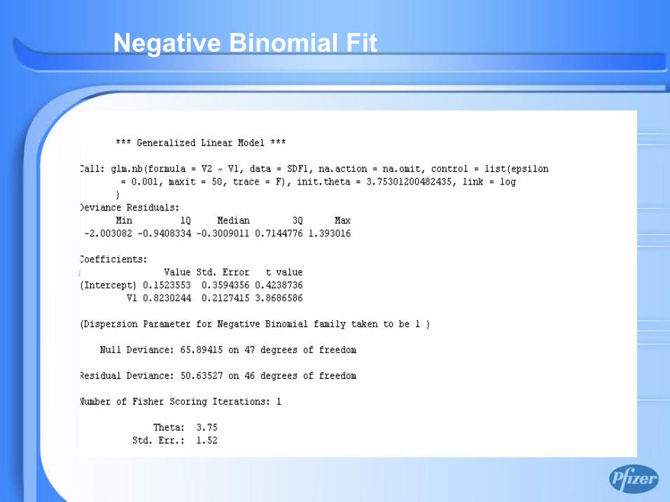
Negative Binomial Fit
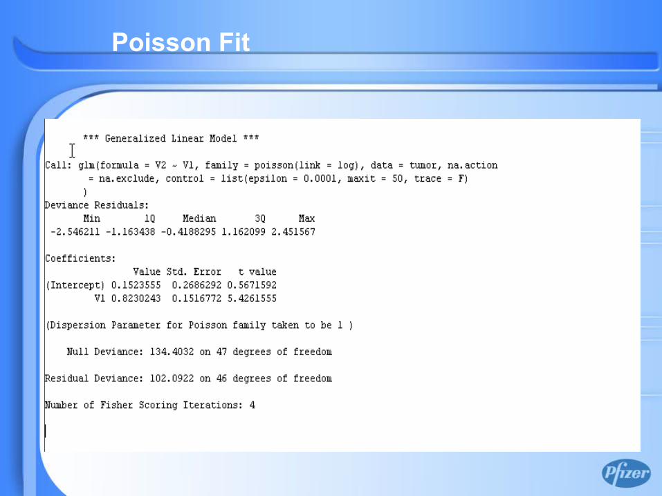
Poisson Fit

R Package
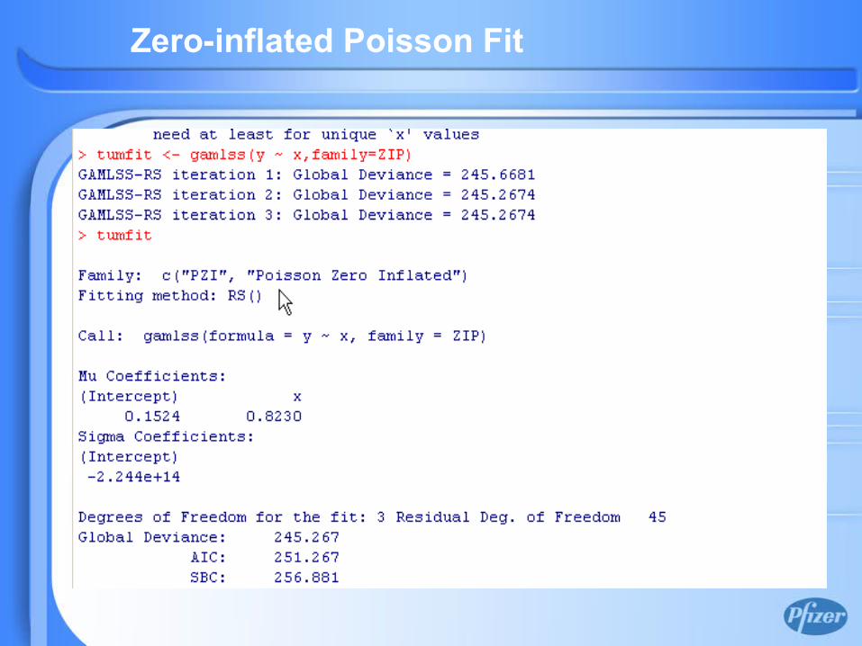
Zero-inflated Poisson Fit
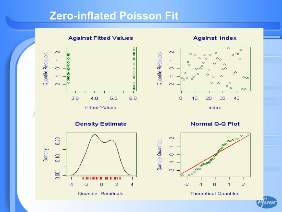
Zero-inflated Poisson Fit

Simulation Results
Simulation with Count Data
• Two independent samples from Poisson distributions are generated– Sample sizes 20, 30 per treatment group – Various Poisson parameters are
considered
• Number of simulations is 500.
Simulation (cont)
• Following tests and model are considered to compare the population means:– Two sample T test– Nonparametric Wilcoxon Rank Sum– Poisson regression model– Negative Binomial model– ZIP model
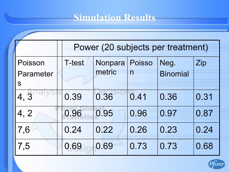
0.680.730.730.690.697,5
0.240.230.260.220.247,6
0.310.360.410.360.394, 3
0.870.970.960.950.964, 2
Zip Neg.Binomial
Poisson
Nonparametric
T-test PoissonParameters
Power (20 subjects per treatment)
Simulation Results
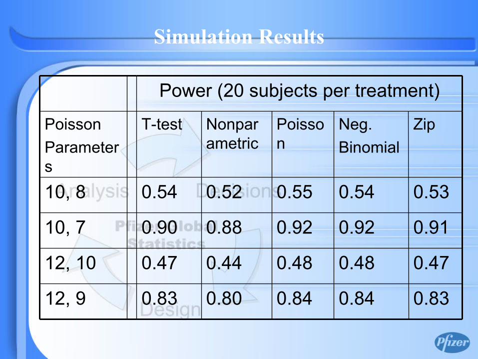
0.830.840.840.800.8312, 9
0.470.480.480.440.4712, 10
0.530.540.550.520.5410, 8
0.910.920.920.880.9010, 7
Zip Neg.Binomial
Poisson
Nonparametric
T-test PoissonParameters
Power (20 subjects per treatment)
Simulation Results
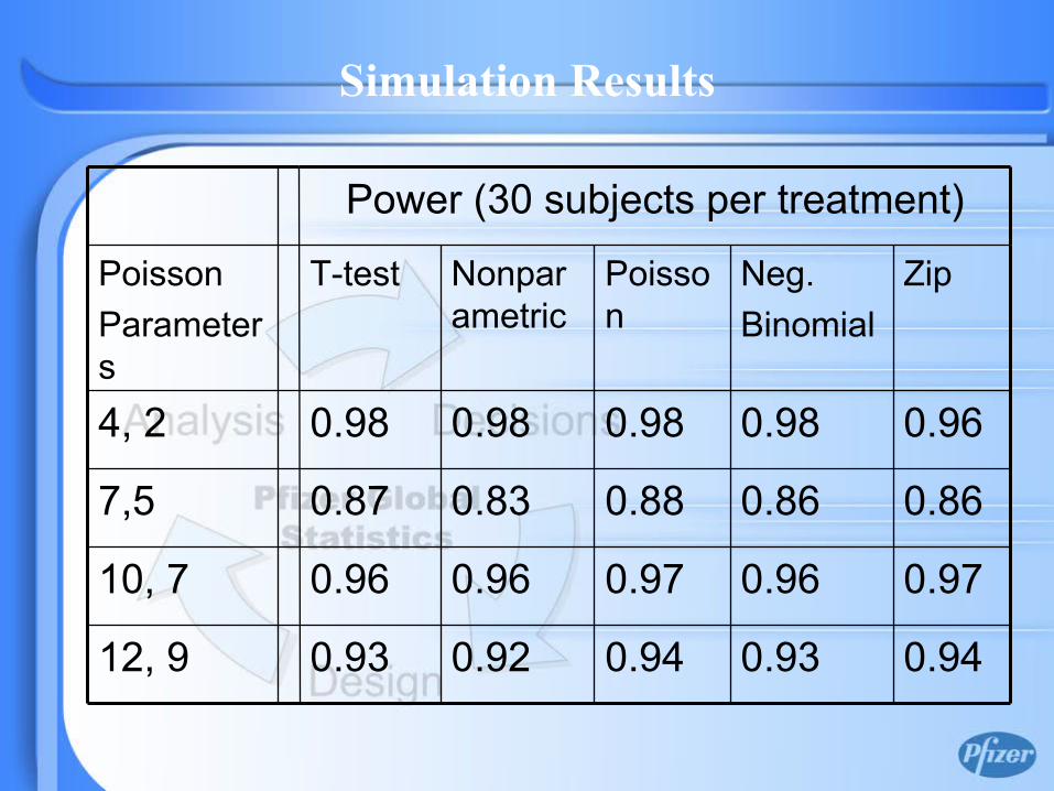
0.940.930.940.920.9312, 9
0.970.960.970.960.9610, 7
0.860.860.880.830.877,5
0.960.980.980.980.984, 2
Zip Neg.Binomial
Poisson
Nonparametric
T-test PoissonParameters
Power (30 subjects per treatment)
Simulation Results
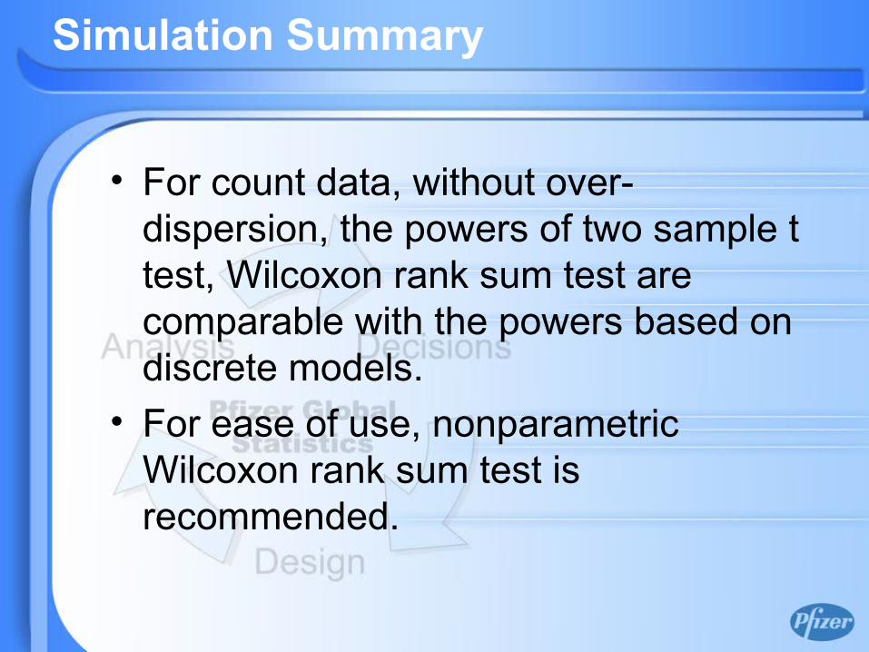
Simulation Summary
• For count data, without over-dispersion, the powers of two sample t test, Wilcoxon rank sum test are comparable with the powers based on discrete models.
• For ease of use, nonparametric Wilcoxon rank sum test is recommended.
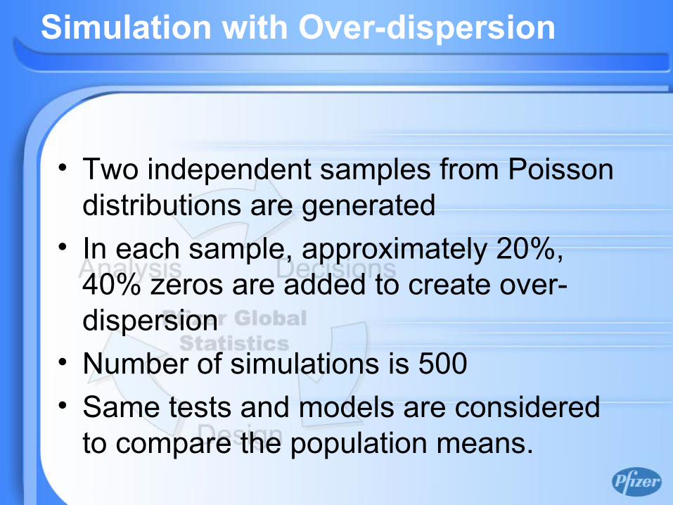
Simulation with Over-dispersion
• Two independent samples from Poisson distributions are generated
• In each sample, approximately 20%, 40% zeros are added to create over-dispersion
• Number of simulations is 500• Same tests and models are considered
to compare the population means.
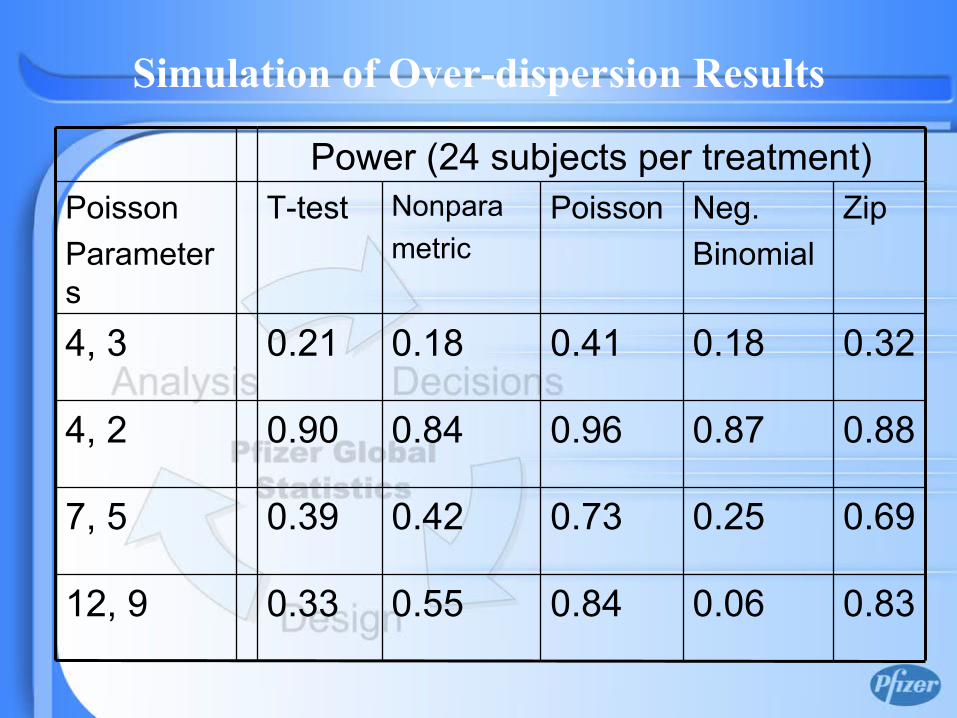
0.830.060.840.550.3312, 9
0.690.250.730.420.397, 5
0.880.870.960.840.904, 2
0.320.180.410.180.214, 3
Zip Neg.Binomial
PoissonNonparametric
T-test PoissonParameters
Power (24 subjects per treatment)
Simulation of Over-dispersion Results
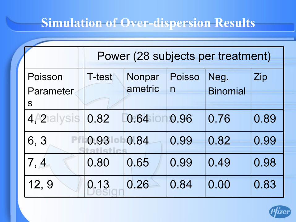
0.980.490.990.650.807, 4
0.830.000.840.260.1312, 9
0.990.820.990.840.936, 3
0.890.760.960.640.824, 2
Zip Neg.Binomial
Poisson
Nonparametric
T-test PoissonParameters
Power (28 subjects per treatment)
Simulation of Over-dispersion Results

0.860.150.890.390.447, 5
0.940.000.940.530.3412, 9
0.990.970.990.970.986, 3
0.970.930.980.880.954, 2
Zip Neg.Binomial
Poisson
Nonparametric
T-test PoissonParameters
Power (42 subjects per treatment)
Simulation of Over-dispersion Results
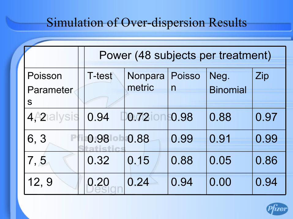
0.860.050.880.150.327, 5
0.940.000.940.240.2012, 9
0.990.910.990.880.986, 3
0.970.880.980.720.944, 2
Zip Neg.Binomial
Poisson
Nonparametric
T-test PoissonParameters
Power (48 subjects per treatment)
Simulation of Over-dispersion Results
Simulation Summary (over-dispersion)
• In cases of over-dispersion, Poisson regression model produces highest power consistently followed by ZIP model.
• When the means are lower (closer to zero), power based on t-test and nonparametric tests are not too low compared to the power from the Poisson regression model.
Simulation Summary (over-dispersion)
• When the means are higher, Poisson regression and ZIP model are clearly the winners.
• Unless over-dispersion is rather high (50% or more) and the means are high (i. e., the variability in the sample is very high) ZIP model is not necessary!

• What is the best model?• A natural way to measure the performance of a fitted
candidate model is by using a model selection criterion that scores every fitted model in a candidate class.
• Examine the effectiveness of Poisson and ZIP models to accommodate overdispersion using Poisson plots, score statistics, and model selection criteria.
Model Comparison for Zero-Inflated Data
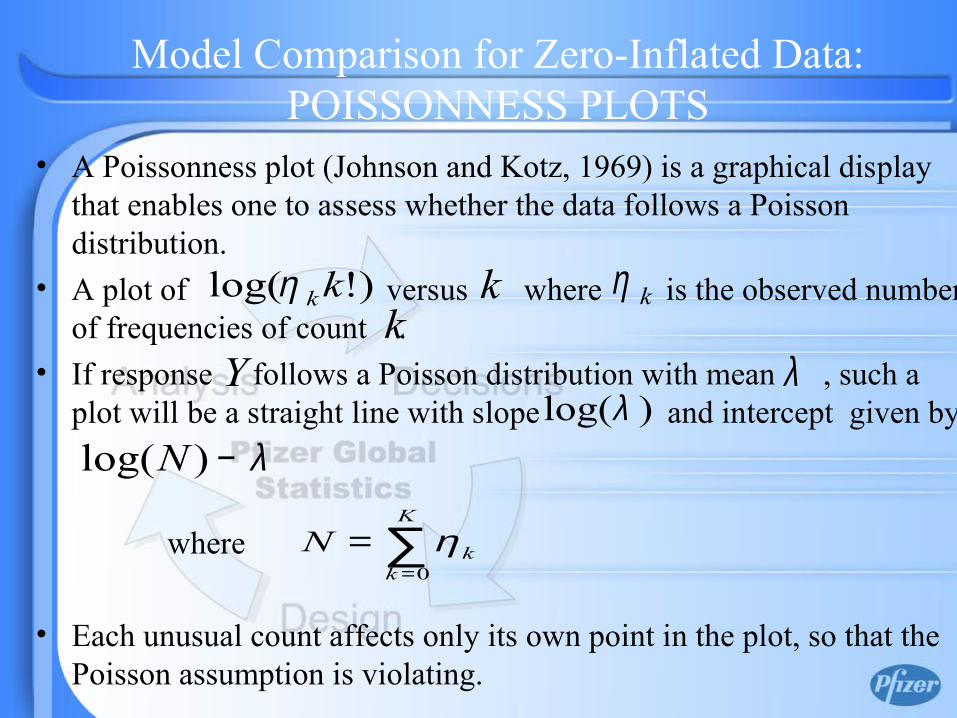
• A Poissonness plot (Johnson and Kotz, 1969) is a graphical display that enables one to assess whether the data follows a Poisson distribution.
• A plot of versus where is the observed number of frequencies of count .
• If response follows a Poisson distribution with mean , such a plot will be a straight line with slope and intercept given by
where
• Each unusual count affects only its own point in the plot, so that the Poisson assumption is violating.
)!log( kkη k kηk
Y λ)log(λ
λ−)log(N
∑=
=K
kkN
0
η
Model Comparison for Zero-Inflated Data:POISSONNESS PLOTS
Model Comparison for Zero-Inflated Data:Score Statistic (Broek, 1995)
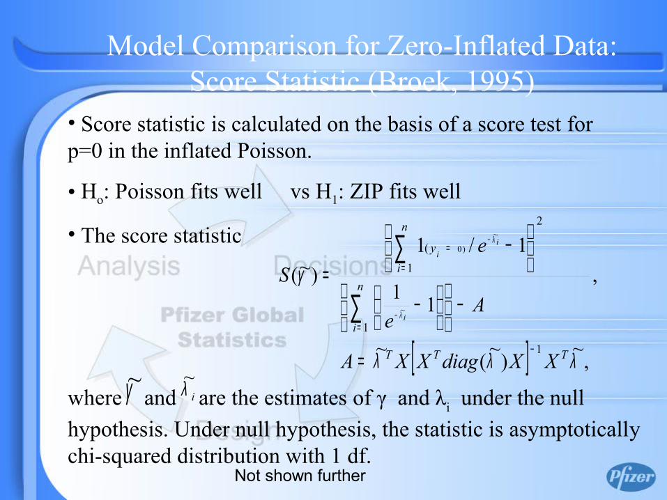
• Score statistic is calculated on the basis of a score test for p=0 in the inflated Poisson.
• Ho: Poisson fits well vs H1: ZIP fits well
• The score statistic
where and are the estimates of γ and λi under the null hypothesis. Under null hypothesis, the statistic is asymptotically chi-squared distribution with 1 df.
[ ]
,
,~)~(~
11
1/1)~(
1
1
2
1(
~
~
)0
λλλ
γ
λ
λ
TTT
n
i
n
iy
XXdiagXXA
Ae
eS
i
ii
−
=
=
=
=
−
−
−
=
∑
∑
−
−
γ~ iλ~
Not shown further
Model Comparison for Zero-Inflated Data
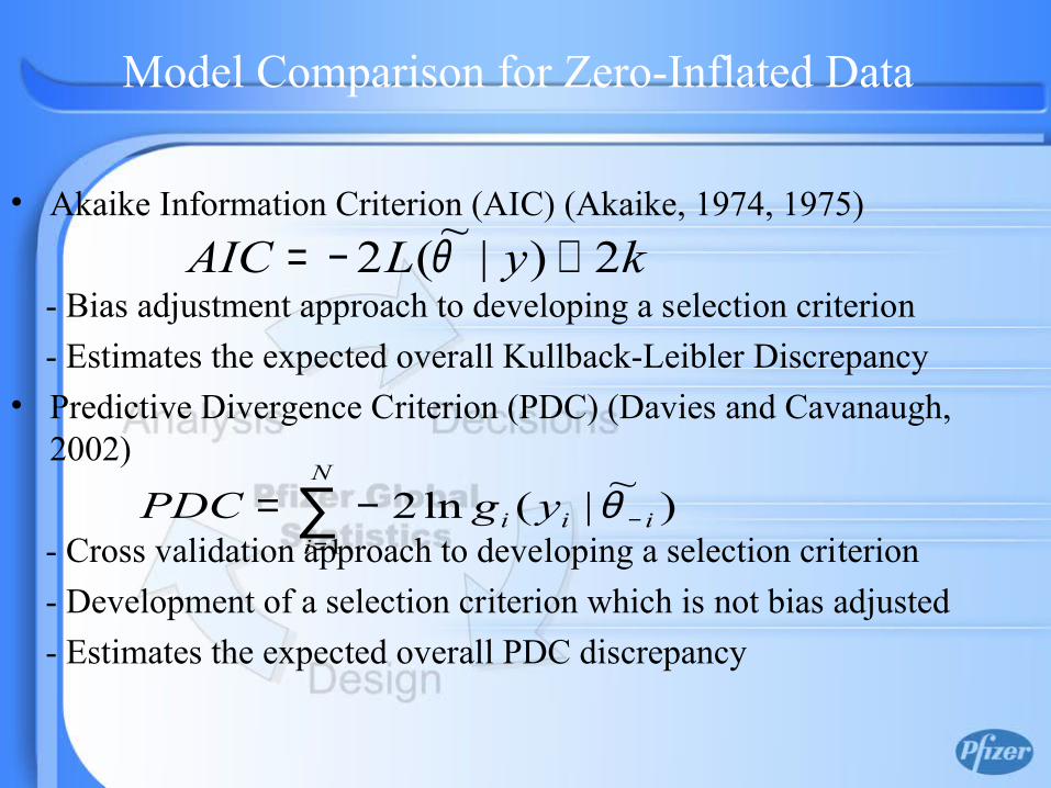
• Akaike Information Criterion (AIC) (Akaike, 1974, 1975)
- Bias adjustment approach to developing a selection criterion - Estimates the expected overall Kullback-Leibler Discrepancy• Predictive Divergence Criterion (PDC) (Davies and Cavanaugh,
2002)
- Cross validation approach to developing a selection criterion - Development of a selection criterion which is not bias adjusted - Estimates the expected overall PDC discrepancy
kyLAIC 2)|~(2 +−= θ
∑=
−−=N
iiii ygPDC
1)~|(ln2 θ
Simulation Schemes
• Scheme I– No covariate
• Scheme II– Single covariate
• Scheme III– Multiple covariates
• Simulation details are not provided here
• Model comparisons were made

POISSONAIC ZIPAIC
0 10 20 30 40 50 60 70 80 90 100
0
100
200
300
400
ZERO
AIC
(Lambda=2)
POISSON_AIC ZIP_AIC
0 10 20 30 40 50 60 70 80 90 100
0
500
1000
ZERO
AIC
(Lambda=10)
Poisson ZIP
0 10 20 30 40 50 60 70 80 90
0
100
200
300
400
500
600
ZERO
AIC
(Lambda=5)
Plots of AIC vs ZERO (Without Covariate Case) SIMULATION SCHEME I
POISSON ZIP
1009080706050403020100
400
300
200
100
0
ZERO
PD
C
POISSON ZIP
0 10 20 30 40 50 60 70 80 90 100
0
500
1000
ZERO
PD
C
Poisson ZIP
0 10 20 30 40 50 60 70 80 90
0
100
200
300
400
500
600
ZERO
PD
C
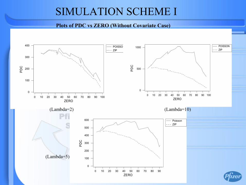
(Lambda=2) (Lambda=10)
(Lambda=5)
Plots of PDC vs ZERO (Without Covariate Case)
SIMULATION SCHEME I
Poisson ZIP
40 50 60 70 80 90 100
0
100
200
300
ZERO
AIC
Poisson ZIP
20 30 40 50 60 70 80 90 100
0
50
100
150
200
250
300
350
ZERO
AIC
Poisson ZIP
40 50 60 70 80 90 100
0
100
200
300
ZERO
PD
C
Poisson ZIP
1009080706050403020
350
300
250
200
150
100
50
0
ZERO
PD
C
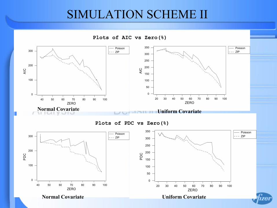
Plots of PDC vs Zero(%)
Plots of AIC vs Zero(%)
Normal Covariate
Normal Covariate
Uniform Covariate
Uniform Covariate
SIMULATION SCHEME II
SUMMARIZATION OF MODEL COMPARISONS IN DIFFERENT CASES
• In case of without covariate model (simulation scheme I), more large the λ is, more certainty is to get “zero” from Bernoulli distribution only. ZIP is more preferable than Poisson model.
• In simulation scheme II, ZIP is better than Poisson. But it seems to the fact that incorporation of covariates increase the tendency of overdispersion irrespective of zero.
• When data simulated directly from Poisson, even for very large amount of zero, Poisson and ZIP are indistinguishable.
Summary of Model Comparisons
• In simulation III scheme (not shown here), we looked at single and two covariates in ZIP model (making it closer to Poisson Regression
• In simulation scheme, though from the score statistics, Poisson is preferable compared to ZIP, AIC and PDC values for both models are not so much different.

Poisson counts are not out of the ordinary?
• , 70: 494-499 .