High Technology High School –

Team # 8878 Lincroft, NJ

Coach: Ellen LeBlanc

Students: Eric Jiang, Anjali Nambrath, Arvind Yalavarti, Kevin

Yan, Lori Zhang

Moody’s Mega Math Challenge Finalist, $5,000 Team Prize

***Note: This cover sheet has been added by SIAM to identify the winning team after

judging was completed. Any identifying information other than team # on a Moody’s

Mega Math Challenge submission is a rules violation.

***Note: This paper underwent a light edit by SIAM staff prior to posting.

Team #8878, Page 1 of 20

From Sea to Shining Sea: Looking ahead with the National Park Service

Executive Summary

One of America’s greatest blessings is often among its most overlooked: its national parks.America’s national parks stand as a hallmark of natural beauty, with unparalleled geo-graphic and biological diversity. However, in light of worrying global warming trends, thewell-being and longevity of the parks must be considered. In particular, our coastal parksare directly at risk due to rising sea levels and climate change. Our model seeks to predictcoastal parks’ vulnerability to these factors.

First, we developed a model to predict future sea level changes for five coastal parks. Globalaverage sea level is affected by two main factors: thermal expansion of water and glaciermeltwater. However, local sea levels vary due to location-specific land uplift resulting fromisostatic rebound and tectonic plate activity. Taking into account these factors, a functionwas created to predict the yearly change in local sea level.

We used our model to generate a corresponding sea level change risk rating of high, medium,or low for each of the five coastal parks. Over a time frame ranging from 10 to 50 years,our model predicts a medium sea level change risk rating for Acadia, Cape Hatteras, andPadre Island. This signifies that these parks may endure moderately damaging conse-quences (infrastructure damage and wildlife loss). On the other hand, Olympic NationalPark and Kenai Fjords are predicted to be at low risk for sea level change.

In addition to sea level rise, parks are susceptible to a variety of other climate-based fac-tors. Thus, we developed a model that yields a vulnerability score which offers a broaderperspective on a park’s susceptibility to climate change. This model incorporates individ-ually calculated vulnerability scores of each park to factors such as natural disasters, bio-diversity shifts, and temperature change. These values are then weighted and summed togenerate the final vulnerability score, which ranges from 0 (least vulnerable) to 10 (mostvulnerable). Hatteras has the highest vulnerability score of 4.47, while Padre has the low-est score of 3.12. Holistically, each park has a relatively low score, signifying that none areextremely vulnerable to climate change.

Given all the threats America’s national parks face, it is important that the Parks Serviceapportion its funds to best address its various concerns. However, these are not limitedto climate concerns. The Parks Service also works on increasing environmental awareness,promoting a love of nature in younger generations, and is also responsible for simple main-tenance and cannot solely address climate change risk. In order to determine how best theParks Service should use its funds, we created a projection of yearly visitors to each parkin order to determine whether more money should be directed to promotion and increas-ing public interest, or to park maintenance and mitigation of the consequences of climatechange. We found that attendance is projected to increase fairly steadily, so funds setaside for upkeep and preservation of parks should not be decreased.

The future of America’s national parks is of the utmost importance. Our models attemptto provide answers to pressing questions regarding sea levels, climate change vulnerability,and attendance. These models seek to shed light on how the park system may change inthe upcoming years and provide guidance to the NPS, ensuring that future generationswill also have to opportunity experience the beauty of America’s national parks.

CONTENTS Team #8878, Page 2 of 20

Contents

1 Problem Restatement 3

2 Tides of Change 3

2.1 Assumptions and Justifications . . . . . . . . . . . . . . . . . . . . . . . . . . . . 3

2.2 Model Overview . . . . . . . . . . . . . . . . . . . . . . . . . . . . . . . . . . . . . 4

2.3 Global Factors Affecting SLR . . . . . . . . . . . . . . . . . . . . . . . . . . . . . 4

2.4 Local Factors Affecting SLR . . . . . . . . . . . . . . . . . . . . . . . . . . . . . . 6

2.5 SLR Model . . . . . . . . . . . . . . . . . . . . . . . . . . . . . . . . . . . . . . . . 7

2.5.1 Sensitivity Analysis . . . . . . . . . . . . . . . . . . . . . . . . . . . . . . . 8

2.6 Assessing Sea Level Change Risk . . . . . . . . . . . . . . . . . . . . . . . . . . . 8

2.7 Forecasting over 100 Years . . . . . . . . . . . . . . . . . . . . . . . . . . . . . . . 9

2.8 Model Revisions . . . . . . . . . . . . . . . . . . . . . . . . . . . . . . . . . . . . . 9

3 The Coast Is Clear? 10

3.1 Model Overview . . . . . . . . . . . . . . . . . . . . . . . . . . . . . . . . . . . . . 10

3.2 Assumptions and Justifications . . . . . . . . . . . . . . . . . . . . . . . . . . . . 10

3.3 Contributing Factors to CVS . . . . . . . . . . . . . . . . . . . . . . . . . . . . . . 11

3.4 Model Revisions . . . . . . . . . . . . . . . . . . . . . . . . . . . . . . . . . . . . . 14

4 Let Nature Take Its Course? 14

4.1 Assumptions and Justifications . . . . . . . . . . . . . . . . . . . . . . . . . . . . 14

4.2 Visitor Model Overview . . . . . . . . . . . . . . . . . . . . . . . . . . . . . . . . . 15

4.3 Socioeconomic Model . . . . . . . . . . . . . . . . . . . . . . . . . . . . . . . . . . 15

4.3.1 Probability of Visiting a Park . . . . . . . . . . . . . . . . . . . . . . . . . 15

4.3.2 Population Model . . . . . . . . . . . . . . . . . . . . . . . . . . . . . . . . 16

4.3.3 Scaling the Socioeconomic Model . . . . . . . . . . . . . . . . . . . . . . . 17

4.4 National Park Service Recommendations . . . . . . . . . . . . . . . . . . . . . . 18

4.5 Model Revisions . . . . . . . . . . . . . . . . . . . . . . . . . . . . . . . . . . . . . 18

5 Conclusion 18

Team #8878, Page 3 of 20

1 Problem Restatement

The problem we are tasked with addressing is as follows:

1. Predict sea level changes over the next 10, 20, and 50 years. Assign a sea level changerisk rating of high, medium, or low to each of the five parks.

2. Taking into account the likelihood and severity of climate-related events in eachpark, develop a model that can yield a climate-vulnerability score for any NPS coastalunit.

3. Predict long-term changes in visitors for each of the five parks. Using this prediction,advise NPS on the allocation of future financial resources.

2 Tides of Change

Global sea levels have been rising faster in recent decades than ever before. The accelera-tion of sea level change is one of many manifestations of increasingly problematic climatechange, which threatens the ecological stability of our planet. The rising sea level posesan especially dire concern to coastal environments and threatens several United States na-tional parks located near seashores. In order to assess the level of risk that these parksface as a result of rising oceans, it is first necessary to develop a model for local sea levelincreases over time.

2.1 Assumptions and Justifications

In order to generalize our model for local sea level increases, we made the following as-sumptions:

1. The surface area of the ocean will not change significantly when the vol-ume increases. While the surface area does increase slightly, this was found to beinsignificant when taking into consideration the volume of the entire ocean.

2. The total volume of the Earth’s glaciers can be represented by rectangu-lar prism with a square base. This facilitates volume calculations and roughlyapproximates the physical form of individual glaciers.

3. The height of the rectangular prism is 2.1 km. This is the average height ofthe major ice caps located at the poles [11].

4. The density of the Earth’s crust increases proportionally with depth. Thisassumption was necessary in order to simplify calculations for the isostatic equilib-rium of land masses, used in Part 2.4.

5. The rate of tectonic activity is constant over time. Because tectonic platesmove so slowly, the difference in movement from year to year is unlikely to differ sig-nificantly. This simplifies calculations for land uplift, also used in Part 2.4.

2.2 Model Overview Team #8878, Page 4 of 20

2.2 Model Overview

There are a multitude of factors that lead to changing sea levels, but we chose to focus ona few major ones. While wind patterns, ocean current trends, and groundwater do affectsea level changes, they do not contribute as much as other, more dominating phenomena.We chose to break up regional changes in mean sea level (SLR) into changes caused byglobal factors, changes, and local factors. The main global factors were thermal expansionof water and the melting of glaciers and ice caps due to increasing global temperatures.The predominant local factor was land uplift due to tectonic and glacial activity. Combin-ing these three factors into one equation gives us

SLR = TE +MI −U, (1)

where TE is the change due to thermal expansion, MI is the change due to melting ice,and U is the land uplift factor.

2.3 Global Factors Affecting SLR

Thermal ExpansionAs water heats up, it expands. Since the global temperature is increasing, a major factorthat plays into SLR is the simple increase in volume of the warmer oceans [6].

The change in the volume of the mean global sea level due to thermal expansion can becalculated using two distinct equations which, when set equal to each other, can outputthe change in depth, ∆D, of the global sea level due to thermal expansion.

In physics, volumetric thermal expansion can be calculated by

∆V = βVO∆T, (2)

where ∆V is the change in the ocean’s volume, β is the coefficient coefficient of volumethermal expansion, VO is the initial volume, and ∆T is the change in global temperature.

For our model, we substituted VO with Di ∗ SA, where Di is the initial depth of the oceanand SA is the surface area of the ocean. This is a valid substitution as Volume = Depth ∗Surface Area. Di is the max depth at which temperature changes occur under the oceansurface. This was determined to be 1000m, the lower limit of the thermocline, which is thetransition layer between warmer mixed water at the ocean’s surface and the colder, deeperwater down below [22]. From research, β was determined to be 1.5 ∗ 10−4°C−1, which isbased on a mean salinity of 35 parts per thousand and a mean upper ocean temperature of10°C [23].

Finally, ∆T was calculated by performing an exponential regression on historical temper-ature data. While this regression does not account for the sawtooth shape of the data, itdoes demonstrate the accelerating increase in temperature that the data show. The regres-sion equation was found to be

∆T = 0.00106 ∗ e0.0014t, (3)

where t is the current year.

2.3 Global Factors Affecting SLR Team #8878, Page 5 of 20

The change in the ocean’s volume can also be calculated by

∆V = SA ∗∆D, (4)

where ∆D is the change in depth of the ocean.

By setting the two equations equal to each other and substituting the calculated values forSA and ∆T , we get

SA ∗∆D = β ∗ (Di ∗ SA)(0.00106 ∗ e0.0014t). (5)

Cancelling out SA, substituting the known values for β and Di, and solving for ∆D, weget

∆D = 0.000159 ∗ e0.0014t ∗ 1000, (6)

an equation for the yearly change in sea level (∆D) in mm due to thermal expansion as afunction of time t, the current year.

Glacier Melting

Glacier melt is another major factor that contributes to SLR. When glaciers (includingice caps and sheets at the poles) melt, a large volume of water is added to the ocean waterbody.

To find the change in volume per year Vn − Vn+1, a 3rd order polynomial regression wasrun on the change in average thickness (m) of the glaciers with respect to years since 1945.In order to validate the results of the regression, we examined the residuals and found arandom scatter. This suggests that the regression model was efficient.

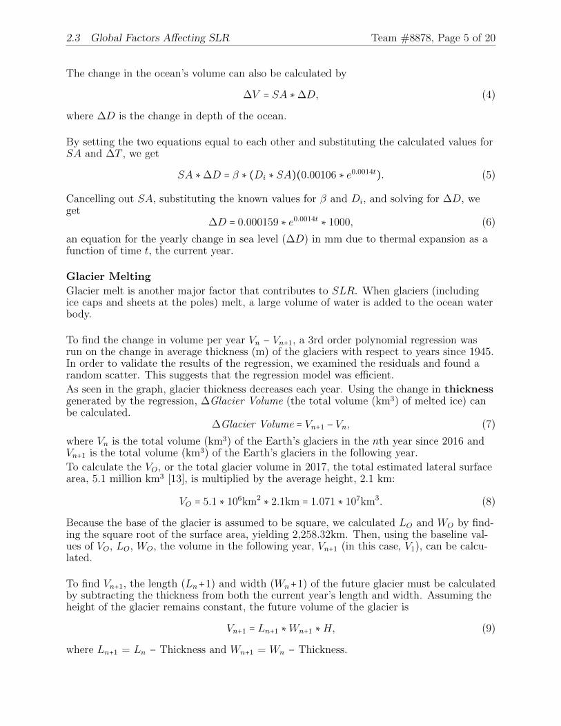
As seen in the graph, glacier thickness decreases each year. Using the change in thicknessgenerated by the regression, ∆Glacier Volume (the total volume (km3) of melted ice) canbe calculated.

∆Glacier Volume = Vn+1 − Vn, (7)

where Vn is the total volume (km3) of the Earth’s glaciers in the nth year since 2016 andVn+1 is the total volume (km3) of the Earth’s glaciers in the following year.

To calculate the VO, or the total glacier volume in 2017, the total estimated lateral surfacearea, 5.1 million km3 [13], is multiplied by the average height, 2.1 km:

VO = 5.1 ∗ 106km2 ∗ 2.1km = 1.071 ∗ 107km3. (8)

Because the base of the glacier is assumed to be square, we calculated LO and WO by find-ing the square root of the surface area, yielding 2,258.32km. Then, using the baseline val-ues of VO, LO, WO, the volume in the following year, Vn+1 (in this case, V1), can be calcu-lated.

To find Vn+1, the length (Ln+1) and width (Wn+1) of the future glacier must be calculatedby subtracting the thickness from both the current year’s length and width. Assuming theheight of the glacier remains constant, the future volume of the glacier is

Vn+1 = Ln+1 ∗Wn+1 ∗H, (9)

where Ln+1 = Ln − Thickness and Wn+1 = Wn − Thickness.

2.4 Local Factors Affecting SLR Team #8878, Page 6 of 20

Figure 1: Graphical Depiction of Change in Glacier Volume in 1 Year

Finally, once Vn and Vn+1 are calculated, the recursive function calculates MI, the SLRcontributed by glacier melt per year.

MI = (∆Glacier Volume)Kglacier

(10)

where ∆Glacier Volume is the total volume (km3) of melted ice and Kglacier = 392.277.Kglacier signifies that for every 392.277km3 of glacier melt, there will be 1 mm of SLR.

2.4 Local Factors Affecting SLR

Isostatic Rebound and Tectonic Plate Activity

Land uplift is an increase in absolute land levels due to various geological phenomena. Thetwo major causes of land uplift we considered were isostatic rebound and tectonic plateactivity. Isostatic rebound is an increase in the level of land masses that were weigheddown by ice sheets and glaciers. As the ice melts, the weight is lifted, and the level of theland increases. Tectonic plate activity can lead to an increase in land levels at subduc-tion zones, which occur predominantly at coastal areas. At subduction zones, a continen-tal tectonic plate is pushed upwards by an oceanic plate sinking into the Earth’s mantle.

These two types of land uplift affect the five parks under consideration differently. AcadiaNational Park is not located at a subduction zone, so isostatic rebound is the main causeof land uplift. Isostatic rebound essentially entails the return of land masses to equilibriumafter a deformation. We modeled isostatic rebound linearly using historical data, estimat-ing that the rebound can be approximated by Hooke’s Law. The yearly rebound value wasestimated to be 0.15 mm a year.

Cape Hatteras National Seashore and Padre Island National Seashore are both affectedsimilarly because they are both located on barrier islands. Neither is located near a tec-tonic plate boundary or near glacial activity, so we determined that both experience negli-gible land uplift.

Kenai Fjords National Park is located in southern Alaska, which has been experiencingsignificant uplift as a result of glacial melting and tectonic activity. However, copious data

2.5 SLR Model Team #8878, Page 7 of 20

exist documenting the effects of these changes. A study conducted at the University ofAlaska at Fairbanks found that the rate of vertical uplift in Homer, a town located onthe same peninsula as Kenai Fjords National Park, was 9.4 mm upwards per year. Thisis much more uplift than has been observed in other locations around the world, and hasactually led to a decline in the relative sea level in southern Alaska. The rate of uplift hasbeen fairly constant over the past twenty years, and so we expect it to remain the samegoing forwards.

Olympic National Park is located on Washington’s Olympic Peninsula, which is on anaccretionary wedge, a special kind of subduction zone. Therefore the sort of land upliftit experiences is nearly entirely tectonic. The rate of uplift was measured in 2001 by theYale Geology Department to be 0.5 mm per year. Using the same assumption as for KenaiFjords, we expect this number to be the same in the future.

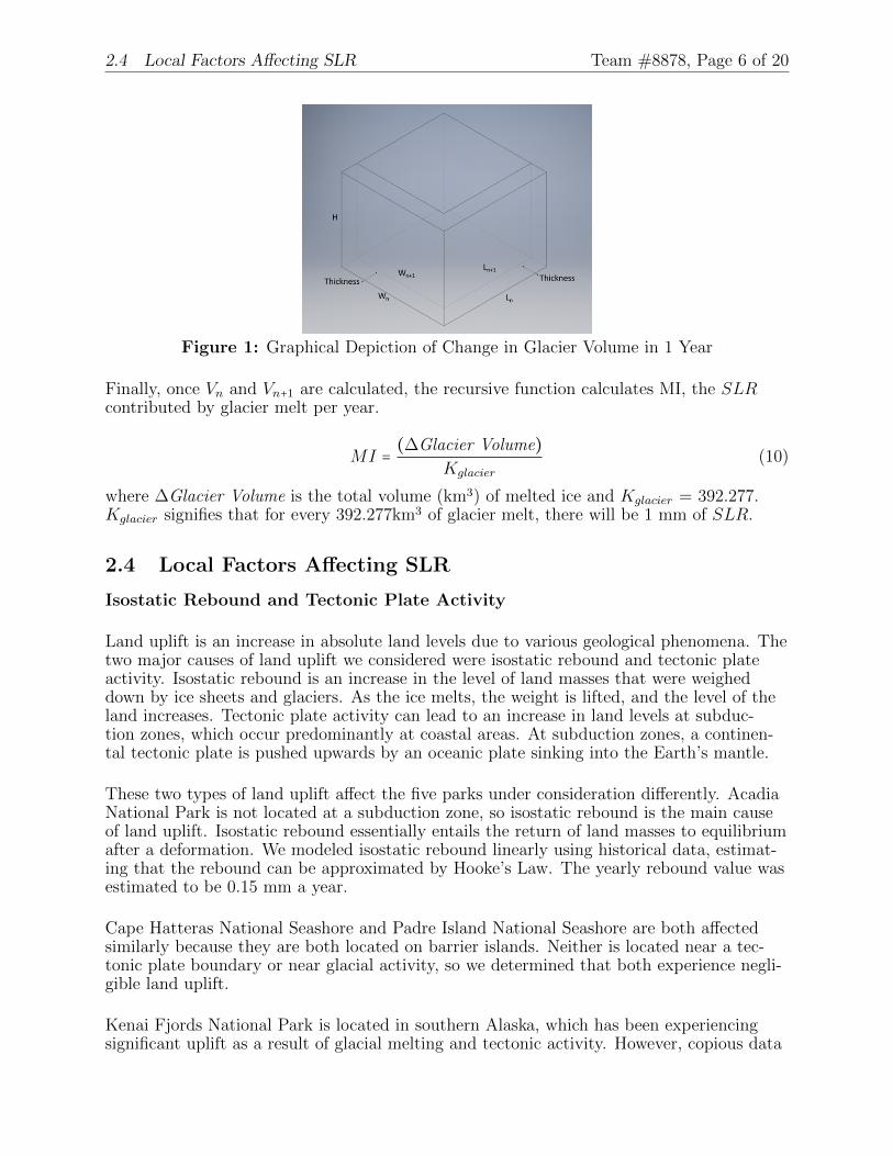
Table 1: Yearly Land Uplift Rate (U) for National Parks

National ParkYearly Land UpliftRate (mm/year)

Acadia 0.15Cape Hatteras 0.0Kenai Fjords 9.4

Olympic 0.5Padre Island 0.0

2.5 SLR Model

By combining the equations from the aforementioned factors, we get the final SLR modelfor yearly sea level increases in years:

SLR = (0.000159 ∗ e0.0014t) + (∆Glacier Volume

392.277) −U. (11)

Projections

The net change in sea level over n years can be determined using a sum of the yearly changein each of those years:

Final Year

∑i=2016

TEi +MIi −U, (12)

where Final Year is the current year. We summed TE and U using two separate summa-tions and programmatically summed MI by writing a recursive Java program. Runningthe model on the 5 given National Parks using Table 1 for the U values gives us the netchange in sea level over the 10, 20, and 50 year periods. These outputs are shown below.

Table 2: Net Change in Sea Level (mm) for National Parks

National Park 10 Years 20 Years 50 Years

Acadia 38.0611 78.679 250.40Cape Hatteras 39.711 81.829 258.054Kenai Fjords −63.689 −115.571 −221.346

Olympic 34.211 71.329 232.554Padre Island 39.711 81.829 258.054

2.6 Assessing Sea Level Change Risk Team #8878, Page 8 of 20

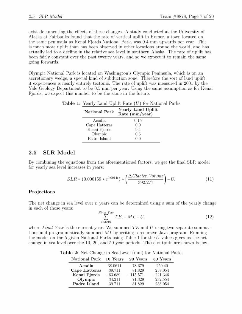
2.5.1 Sensitivity Analysis

In order to determine which variables have the greatest impact on the net change in sealevel, we took one factor and shifted its value by 5% to see the resulting net change in sealevel.

Table 3: Sensitivity Analysis Values

Factor Shift % 10 Years 20 Years 50 Years

β ±5.00 ±0.00806 ±0.00818 ±0.008526kGlacier ±5.00 ±0.02499 ±0.027078 ±0.06041

As the shifts in net change in sea level are so small, this supports our model since smallchanges in factors do not have a profound impact on the overall output of the model.

2.6 Assessing Sea Level Change Risk

Defining Risk Thresholds

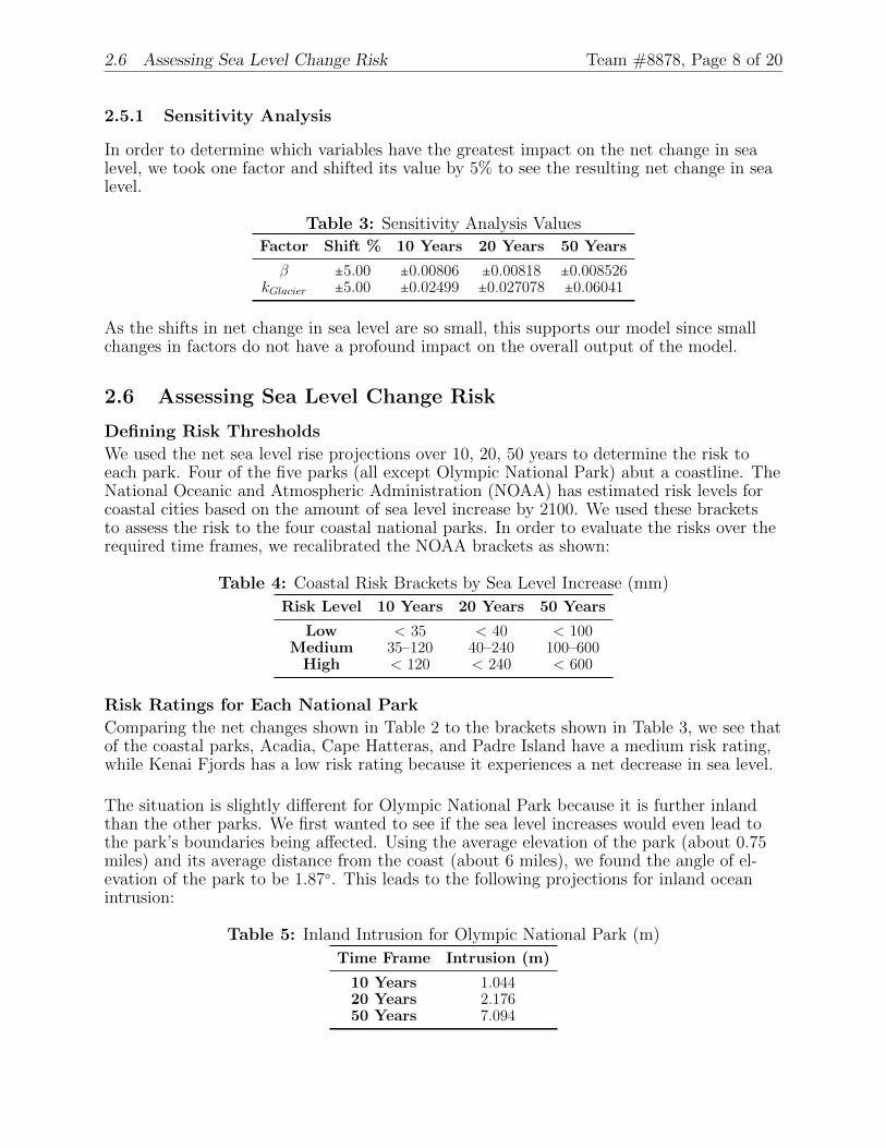
We used the net sea level rise projections over 10, 20, 50 years to determine the risk toeach park. Four of the five parks (all except Olympic National Park) abut a coastline. TheNational Oceanic and Atmospheric Administration (NOAA) has estimated risk levels forcoastal cities based on the amount of sea level increase by 2100. We used these bracketsto assess the risk to the four coastal national parks. In order to evaluate the risks over therequired time frames, we recalibrated the NOAA brackets as shown:

Table 4: Coastal Risk Brackets by Sea Level Increase (mm)

Risk Level 10 Years 20 Years 50 Years

Low < 35 < 40 < 100Medium 35–120 40–240 100–600

High < 120 < 240 < 600

Risk Ratings for Each National Park

Comparing the net changes shown in Table 2 to the brackets shown in Table 3, we see thatof the coastal parks, Acadia, Cape Hatteras, and Padre Island have a medium risk rating,while Kenai Fjords has a low risk rating because it experiences a net decrease in sea level.

The situation is slightly different for Olympic National Park because it is further inlandthan the other parks. We first wanted to see if the sea level increases would even lead tothe park’s boundaries being affected. Using the average elevation of the park (about 0.75miles) and its average distance from the coast (about 6 miles), we found the angle of el-evation of the park to be 1.87○. This leads to the following projections for inland oceanintrusion:

Table 5: Inland Intrusion for Olympic National Park (m)

Time Frame Intrusion (m)

10 Years 1.04420 Years 2.17650 Years 7.094

2.7 Forecasting over 100 Years Team #8878, Page 9 of 20

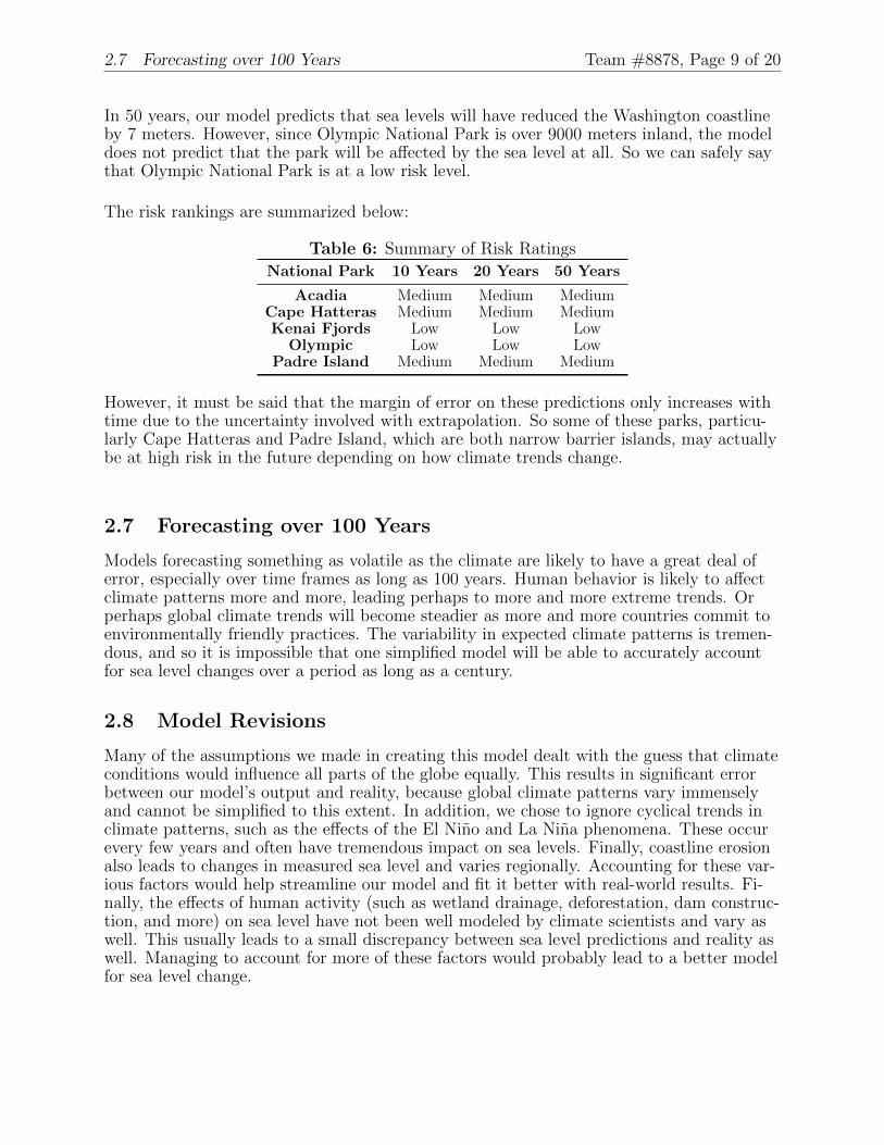
In 50 years, our model predicts that sea levels will have reduced the Washington coastlineby 7 meters. However, since Olympic National Park is over 9000 meters inland, the modeldoes not predict that the park will be affected by the sea level at all. So we can safely saythat Olympic National Park is at a low risk level.

The risk rankings are summarized below:

Table 6: Summary of Risk Ratings

National Park 10 Years 20 Years 50 Years

Acadia Medium Medium MediumCape Hatteras Medium Medium MediumKenai Fjords Low Low Low

Olympic Low Low LowPadre Island Medium Medium Medium

However, it must be said that the margin of error on these predictions only increases withtime due to the uncertainty involved with extrapolation. So some of these parks, particu-larly Cape Hatteras and Padre Island, which are both narrow barrier islands, may actuallybe at high risk in the future depending on how climate trends change.

2.7 Forecasting over 100 Years

Models forecasting something as volatile as the climate are likely to have a great deal oferror, especially over time frames as long as 100 years. Human behavior is likely to affectclimate patterns more and more, leading perhaps to more and more extreme trends. Orperhaps global climate trends will become steadier as more and more countries commit toenvironmentally friendly practices. The variability in expected climate patterns is tremen-dous, and so it is impossible that one simplified model will be able to accurately accountfor sea level changes over a period as long as a century.

2.8 Model Revisions

Many of the assumptions we made in creating this model dealt with the guess that climateconditions would influence all parts of the globe equally. This results in significant errorbetween our model’s output and reality, because global climate patterns vary immenselyand cannot be simplified to this extent. In addition, we chose to ignore cyclical trends inclimate patterns, such as the effects of the El Nino and La Nina phenomena. These occurevery few years and often have tremendous impact on sea levels. Finally, coastline erosionalso leads to changes in measured sea level and varies regionally. Accounting for these var-ious factors would help streamline our model and fit it better with real-world results. Fi-nally, the effects of human activity (such as wetland drainage, deforestation, dam construc-tion, and more) on sea level have not been well modeled by climate scientists and vary aswell. This usually leads to a small discrepancy between sea level predictions and reality aswell. Managing to account for more of these factors would probably lead to a better modelfor sea level change.

Team #8878, Page 10 of 20

3 The Coast Is Clear?

3.1 Model Overview

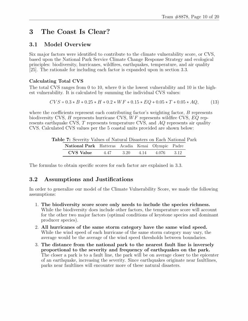
Six major factors were identified to contribute to the climate vulnerability score, or CVS,based upon the National Park Service Climate Change Response Strategy and ecologicalprinciples: biodiversity, hurricanes, wildfires, earthquakes, temperature, and air quality[25]. The rationale for including each factor is expanded upon in section 3.3.

Calculating Total CVS

The total CVS ranges from 0 to 10, where 0 is the lowest vulnerability and 10 is the high-est vulnerability. It is calculated by summing the individual CVS values:

CV S = 0.3 ∗B + 0.25 ∗H + 0.2 ∗WF + 0.15 ∗EQ + 0.05 ∗ T + 0.05 ∗AQ, (13)

where the coefficients represent each contributing factor’s weighting factor, B representsbiodiversity CVS, H represents hurricane CVS, WF represents wildfire CVS, EQ rep-resents earthquake CVS, T represents temperature CVS, and AQ represents air qualityCVS. Calculated CVS values per the 5 coastal units provided are shown below:

Table 7: Severity Values of Natural Disasters on Each National Park

National Park Hatteras Acadia Kenai Olympic Padre

CVS Value 4.47 3.20 4.14 4.076 3.12

The formulas to obtain specific scores for each factor are explained in 3.3.

3.2 Assumptions and Justifications

In order to generalize our model of the Climate Vulnerability Score, we made the followingassumptions:

1. The biodiversity score score only needs to include the species richness.While the biodiversity does include other factors, the temperature score will accountfor the other two major factors (optimal conditions of keystone species and dominantproducer species).

2. All hurricanes of the same storm category have the same wind speed.While the wind speed of each hurricane of the same storm category may vary, theaverage would be the average of the wind speed thresholds between boundaries.

3. The distance from the national park to the nearest fault line is inverselyproportional to the severity and frequency of earthquakes on the park.The closer a park is to a fault line, the park will be on average closer to the epicenterof an earthquake, increasing the severity. Since earthquakes originate near faultlines,parks near faultlines will encounter more of these natural disasters.

3.3 Contributing Factors to CVS Team #8878, Page 11 of 20

3.3 Contributing Factors to CVS

Biodiversity Score (BS)A leading principle in the theory of genetics and ecological stability is that the greaterdiversity of a system, the more resilient it proves to be. A greater variation in genetic di-versity, and therefore species diversity, leads to an increased ability of the ecosystem asa whole to weather climate disturbances. Therefore, biodiversity is the most weightedfactor at 30%, as it is the greatest contributor to ecological stability and recovery time.

The pure concept of biodiversity is mostly dependent on species richness and may alsobe affected by the optimal conditions of keystone species and dominant producer species.However, for the purposes of determining the CVS score for NPS coastal units, the biodi-versity score will only include the species richness, and the temperature score will accountfor the other two factors.

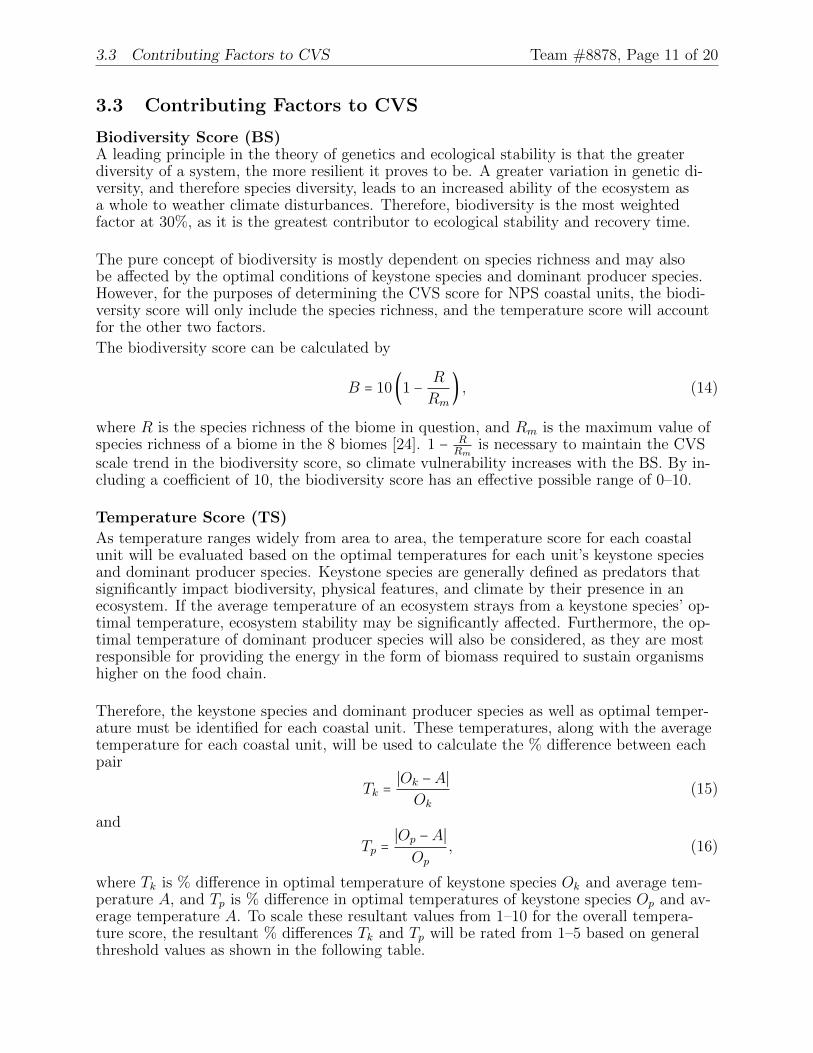
The biodiversity score can be calculated by

B = 10(1 − R

Rm

) , (14)

where R is the species richness of the biome in question, and Rm is the maximum value ofspecies richness of a biome in the 8 biomes [24]. 1 − R

Rmis necessary to maintain the CVS

scale trend in the biodiversity score, so climate vulnerability increases with the BS. By in-cluding a coefficient of 10, the biodiversity score has an effective possible range of 0–10.

Temperature Score (TS)

As temperature ranges widely from area to area, the temperature score for each coastalunit will be evaluated based on the optimal temperatures for each unit’s keystone speciesand dominant producer species. Keystone species are generally defined as predators thatsignificantly impact biodiversity, physical features, and climate by their presence in anecosystem. If the average temperature of an ecosystem strays from a keystone species’ op-timal temperature, ecosystem stability may be significantly affected. Furthermore, the op-timal temperature of dominant producer species will also be considered, as they are mostresponsible for providing the energy in the form of biomass required to sustain organismshigher on the food chain.

Therefore, the keystone species and dominant producer species as well as optimal temper-ature must be identified for each coastal unit. These temperatures, along with the averagetemperature for each coastal unit, will be used to calculate the % difference between eachpair

Tk =∣Ok −A∣Ok

(15)

and

Tp =∣Op −A∣Op

, (16)

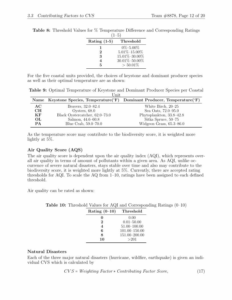
where Tk is % difference in optimal temperature of keystone species Ok and average tem-perature A, and Tp is % difference in optimal temperatures of keystone species Op and av-erage temperature A. To scale these resultant values from 1–10 for the overall tempera-ture score, the resultant % differences Tk and Tp will be rated from 1–5 based on generalthreshold values as shown in the following table.

3.3 Contributing Factors to CVS Team #8878, Page 12 of 20

Table 8: Threshold Values for % Temperature Difference and Corresponding Ratings(1–5)

Rating (1-5) Threshold

1 0%–5.00%2 5.01%–15.00%3 15.01%–30.00%4 30.01%–50.00%5 > 50.01%

For the five coastal units provided, the choices of keystone and dominant producer speciesas well as their optimal temperature are as shown:

Table 9: Optimal Temperature of Keystone and Dominant Producer Species per CoastalUnit

Name Keystone Species, Temperature(°F) Dominant Producer, Temperature(°F)

AC Beavers, 32.0–82.4 White Birch, 20–25CH Oysters, 68.0 Sea Oats, 72.0–95.0KF Black Oystercatcher, 62.0–73.0 Phytoplankton, 33.8–42.8OL Salmon, 44.6–60.8 Sitka Spruce, 50–75PA Blue Crab, 59.0–70.0 Widgeon Grass, 65.3–86.0

As the temperature score may contribute to the biodiversity score, it is weighted morelightly at 5%.

Air Quality Score (AQS)

The air quality score is dependent upon the air quality index (AQI), which represents over-all air quality in terms of amount of pollutants within a given area. As AQI, unlike oc-currence of severe natural disasters, stays stable over time and also may contribute to thebiodiversity score, it is weighted more lightly at 5%. Currently, there are accepted ratingthresholds for AQI. To scale the AQ from 1–10, ratings have been assigned to each definedthreshold.

Air quality can be rated as shown:

Table 10: Threshold Values for AQI and Corresponding Ratings (0–10)

Rating (0–10) Threshold

0 0.002 0.01–50.004 51.00–100.006 101.00–150.008 151.00–200.0010 >201

Natural Disasters

Each of the three major natural disasters (hurricane, wildfire, earthquake) is given an indi-vidual CVS which is calculated by

CV S =Weighting Factor ∗Contributing Factor Score, (17)

3.3 Contributing Factors to CVS Team #8878, Page 13 of 20

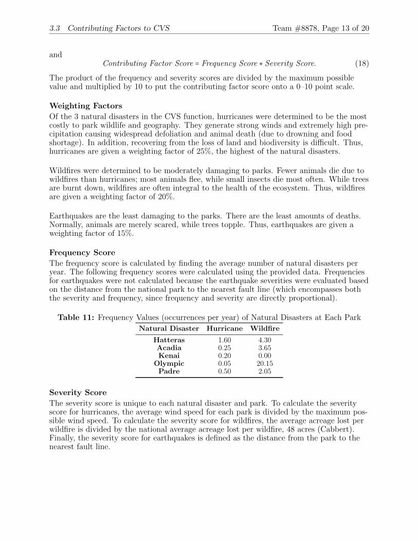
andContributing Factor Score = Frequency Score ∗ Severity Score. (18)

The product of the frequency and severity scores are divided by the maximum possiblevalue and multiplied by 10 to put the contributing factor score onto a 0–10 point scale.

Weighting Factors

Of the 3 natural disasters in the CVS function, hurricanes were determined to be the mostcostly to park wildlife and geography. They generate strong winds and extremely high pre-cipitation causing widespread defoliation and animal death (due to drowning and foodshortage). In addition, recovering from the loss of land and biodiversity is difficult. Thus,hurricanes are given a weighting factor of 25%, the highest of the natural disasters.

Wildfires were determined to be moderately damaging to parks. Fewer animals die due towildfires than hurricanes; most animals flee, while small insects die most often. While treesare burnt down, wildfires are often integral to the health of the ecosystem. Thus, wildfiresare given a weighting factor of 20%.

Earthquakes are the least damaging to the parks. There are the least amounts of deaths.Normally, animals are merely scared, while trees topple. Thus, earthquakes are given aweighting factor of 15%.

Frequency Score

The frequency score is calculated by finding the average number of natural disasters peryear. The following frequency scores were calculated using the provided data. Frequenciesfor earthquakes were not calculated because the earthquake severities were evaluated basedon the distance from the national park to the nearest fault line (which encompasses boththe severity and frequency, since frequency and severity are directly proportional).

Table 11: Frequency Values (occurrences per year) of Natural Disasters at Each Park

Natural Disaster Hurricane Wildfire

Hatteras 1.60 4.30Acadia 0.25 3.65Kenai 0.20 0.00

Olympic 0.05 20.15Padre 0.50 2.05

Severity Score

The severity score is unique to each natural disaster and park. To calculate the severityscore for hurricanes, the average wind speed for each park is divided by the maximum pos-sible wind speed. To calculate the severity score for wildfires, the average acreage lost perwildfire is divided by the national average acreage lost per wildfire, 48 acres (Cabbert).Finally, the severity score for earthquakes is defined as the distance from the park to thenearest fault line.

3.4 Model Revisions Team #8878, Page 14 of 20

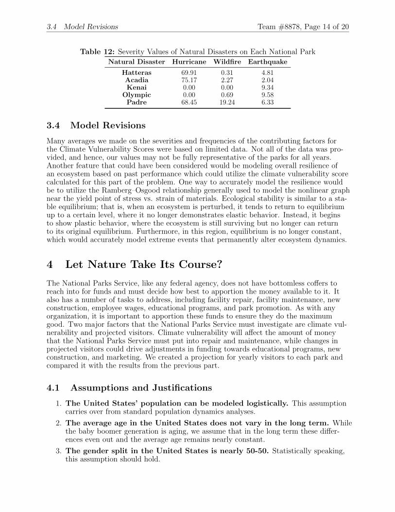
Table 12: Severity Values of Natural Disasters on Each National Park

Natural Disaster Hurricane Wildfire Earthquake

Hatteras 69.91 0.31 4.81Acadia 75.17 2.27 2.04Kenai 0.00 0.00 9.34

Olympic 0.00 0.69 9.58Padre 68.45 19.24 6.33

3.4 Model Revisions

Many averages we made on the severities and frequencies of the contributing factors forthe Climate Vulnerability Scores were based on limited data. Not all of the data was pro-vided, and hence, our values may not be fully representative of the parks for all years.Another feature that could have been considered would be modeling overall resilience ofan ecosystem based on past performance which could utilize the climate vulnerability scorecalculated for this part of the problem. One way to accurately model the resilience wouldbe to utilize the Ramberg–Osgood relationship generally used to model the nonlinear graphnear the yield point of stress vs. strain of materials. Ecological stability is similar to a sta-ble equilibrium; that is, when an ecosystem is perturbed, it tends to return to equilibriumup to a certain level, where it no longer demonstrates elastic behavior. Instead, it beginsto show plastic behavior, where the ecosystem is still surviving but no longer can returnto its original equilibrium. Furthermore, in this region, equilibrium is no longer constant,which would accurately model extreme events that permanently alter ecosystem dynamics.

4 Let Nature Take Its Course?

The National Parks Service, like any federal agency, does not have bottomless coffers toreach into for funds and must decide how best to apportion the money available to it. Italso has a number of tasks to address, including facility repair, facility maintenance, newconstruction, employee wages, educational programs, and park promotion. As with anyorganization, it is important to apportion these funds to ensure they do the maximumgood. Two major factors that the National Parks Service must investigate are climate vul-nerability and projected visitors. Climate vulnerability will affect the amount of moneythat the National Parks Service must put into repair and maintenance, while changes inprojected visitors could drive adjustments in funding towards educational programs, newconstruction, and marketing. We created a projection for yearly visitors to each park andcompared it with the results from the previous part.

4.1 Assumptions and Justifications

1. The United States’ population can be modeled logistically. This assumptioncarries over from standard population dynamics analyses.

2. The average age in the United States does not vary in the long term. Whilethe baby boomer generation is aging, we assume that in the long term these differ-ences even out and the average age remains nearly constant.

3. The gender split in the United States is nearly 50-50. Statistically speaking,this assumption should hold.

4.2 Visitor Model Overview Team #8878, Page 15 of 20

4. Nominal incomes increase steadily with inflation, and yearly inflation oc-curs at 2.0%. In the long term, we expect that economic conditions will remainfairly stable, and that wage increases will not outpace inflation. We assume that U.S.inflation will, in the long term, match expectations and remain at the historic aver-age of about 2.0% [20].

5. The urban population of the United States is growing at a rate of about0.1% yearly. Demographic data show that the urban population of the UnitedStates is on an upwards trend and is increasing on average at this rate. We expectthis trend to continue in the future [21].

6. The area of preserved national parkland will stay the same. Accounting forincreases in preserved parkland would overcomplicate the model because the govern-ment’s attitude towards conservation often varies from administration to administra-tion, making it too hard to accurately predict.

4.2 Visitor Model Overview

A 2007 report published by the United States Department of Agriculture (USDA) pro-vided a model of total yearly national park visitors based on socioeconomic factors [19].We simplified the model to make it more applicable for the long term and added time evo-lution to some of the variables. We took this socioeconomic model for total visitors andscaled it down so that the numbers were consistent with the provided historical data foreach park. This gave us our final projections for each park, up to the year 2050.

4.3 Socioeconomic Model

4.3.1 Probability of Visiting a Park

The USDA report used the following equation, which describes the “wilderness recreationparticipation probability,” or the probability that an American person visits a nationalpark site:

P (visit) = 1

1 + e−XB, (19)

where X is a row matrix containing the means of explanatory variables, and B is a vec-tor containing parameters for each variable. We multiplied the probabilities output by thisfunction by the total U.S. population to get total projected yearly park visitors.

Variables and Their Parameters

The USDA report included a number of variables which affected annual park visitors, butsome of these were far less important than others and less likely to matter in the longterm. We isolated age, gender, U.S. citizenship, membership of an environmental society,average income, distance from nearest national park, and education level as demographicvariables affecting the likelihood of a park visit. The row matrix X contains mean valuesfor these explanatory variables. For example, the average age in the U.S., the proportionof males, the proportion of U.S. citizens, etc. We used census data and values calculatedby the USDA report authors to populate matrix X. Some of the variables, such as incomeand urban population, are more variable over time than others, so we used historical data

4.3 Socioeconomic Model Team #8878, Page 16 of 20

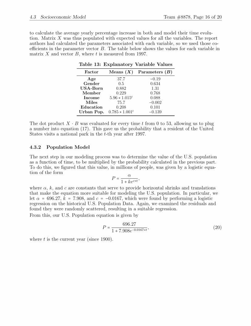
to calculate the average yearly percentage increase in both and model their time evolu-tion. Matrix X was thus populated with expected values for all the variables. The reportauthors had calculated the parameters associated with each variable, so we used those co-efficients in the parameter vector B. The table below shows the values for each variable inmatrix X and vector B, where t is measured from 1997.

Table 13: Explanatory Variable Values

Factor Means (X) Parameters (B)

Age 37.7 −0.19Gender 0.5 0.634

USA-Born 0.882 1.31Member 0.229 0.768Income 5.96 ∗ 1.015t 0.088Miles 75.7 −0.002

Education 0.208 0.101Urban Pop. 0.785 ∗ 1.001t −0.139

The dot product X ⋅ B was evaluated for every time t from 0 to 53, allowing us to pluga number into equation (17). This gave us the probability that a resident of the UnitedStates visits a national park in the t-th year after 1997.

4.3.2 Population Model

The next step in our modeling process was to determine the value of the U.S. populationas a function of time, to be multiplied by the probability calculated in the previous part.To do this, we figured that this value, in millions of people, was given by a logistic equa-tion of the form

P = α

1 + kec∗t ,

where α, k, and c are constants that serve to provide horizontal shrinks and translationsthat make the equation more suitable for modeling the U.S. population. In particular, welet α = 696.27, k = 7.908, and c = −0.0167, which were found by performing a logisticregression on the historical U.S. Population Data. Again, we examined the residuals andfound they were randomly scattered, resulting in a suitable regression.

From this, our U.S. Population equation is given by

P = 696.27

1 + 7.908e−0.0167∗t, (20)

where t is the current year (since 1900).

4.3 Socioeconomic Model Team #8878, Page 17 of 20

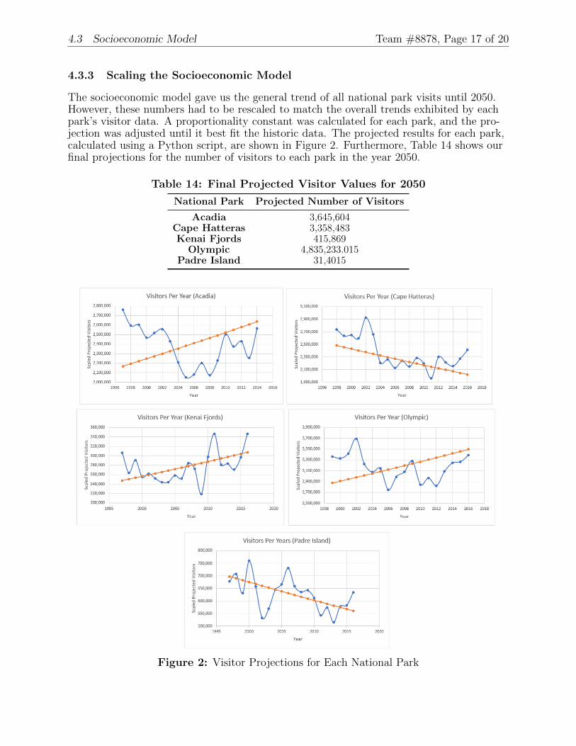
4.3.3 Scaling the Socioeconomic Model

The socioeconomic model gave us the general trend of all national park visits until 2050.However, these numbers had to be rescaled to match the overall trends exhibited by eachpark’s visitor data. A proportionality constant was calculated for each park, and the pro-jection was adjusted until it best fit the historic data. The projected results for each park,calculated using a Python script, are shown in Figure 2. Furthermore, Table 14 shows ourfinal projections for the number of visitors to each park in the year 2050.

Table 14: Final Projected Visitor Values for 2050

National Park Projected Number of Visitors

Acadia 3,645,604Cape Hatteras 3,358,483Kenai Fjords 415,869

Olympic 4,835,233.015Padre Island 31,4015

Figure 2: Visitor Projections for Each National Park

4.4 National Park Service Recommendations Team #8878, Page 18 of 20

4.4 National Park Service Recommendations

Based on our output from the Visitor Projection model, we witness a general upward trendin visitors for each of the national parks. This is substantiated because the National ParkService has been making efforts to increase the attraction of visitors to National Parks[4]. Additionally, in the Budget Justification report released by the National Park Ser-vice for Fiscal Year 2017, we see about 50% of this year’s funds being devoted to promo-tional work, including the Every Kid in a Park program, new construction, and the re-cently adopted Centennial Challenge, which allows parks to fund and complete projectsleft on the back burner. Given the fairly steady increase in projected yearly visitors, ascompared to the dire situation some parks are in, we believe this 50-50 split between fund-ing to new projects and funding for upkeep and maintenance is sufficient, if not too heavilyskewed towards new work. The National Parks Service, we believe, should ensure that thenatural beauty of the United States is preserved for future generations to enjoy and appre-ciate.

4.5 Model Revisions

The visitor projection model is based entirely on demographic and socioeconomic fac-tors, which does not incorporate all of the major relevant factors. Visitor numbers are alsodriven in part by climate change—it has been shown that they vary fairly drastically dur-ing the year with seasonal variations in temperature. These trends are likely to hold up asglobal temperatures increase. Incorporating temperature as a factor would deepen the pro-jection model. In addition, overall climate change and the resultant ecological shifts mightchange people’s motivation to visit a park. If the likelihood of seeing characteristic flora orfauna at a park has been diminished due to climate change, the total number of visitors islikely to be driven down. Incorporating these climate variables into the visitor projectionsis likely to give a more accurate picture of the future of the park system.

5 Conclusion

Our models attempt to provide insight into the future of national parks. First, we soughtto find sea level change risks (high, medium, low) for five coastal parks in the following10, 20, and 50 years. To do so, we developed a model that incorporated factors that con-tribute to global sea level rise (thermal expansion and glacier melt) and local sea levelrise (isostatic rebound and tectonic activity). Ultimately, we determined that Acadia,Cape Hatteras, and Padre Island were at medium risk for sea level change in the giventime frame, while Kenai Fjords and Olympic National Park were at low risk. This modelresponds well to sensitivity analysis, and the sea level change risk predictions hold truewithin the 50-year time frame. Beyond 50 years, it is nearly impossible to accurately pre-dict the temperature and ensuing sea level.

Next, a model that yields any NPS coastal park’s vulnerability score to climate change(on a scale of 0 to 10) was developed. Multiple climate-related factors were weighted andsummed to yield a final climate vulnerability score (CVS). Hatteras has the highest score,4.7, while Padre has the lowest score of 3.12. None of the five coastal parks were deter-mined to be especially vulnerable to climate-related changes, indicating that these parkswill not be terribly affected in the event of climate change. The general model can be used

Team #8878, Page 19 of 20

by the NPS to calculate the CVS of any coastal park.

Finally, a model of projected annual visitors to each park was developed based on socio-economic factors and rescaled to match historic trends for each park. We used the projec-tions to determine that funds should be directed towards preservation and counteractingthe effects of climate change, more so than towards promotion and increasing interest inthe parks. We hope that the National Parks Service can use our findings to plan for thefutures of all national parks, ensuring that America’s unparalleled natural beauty is pre-served for posterity.

REFERENCES Team #8878, Page 20 of 20

References

[1] https://www.fhwa.dot.gov/ohim/onh00/bar8.htm

[2] https://toolkit.climate.gov/topics/coastal/sea-level-rise

[3] https://seer.cancer.gov/popdata/download.html

[4] https://www.nps.gov/aboutus/upload/FY17-NPS-Greenbook-for-website.pdf

[5] http://physics.info/expansion/

[6] http://www.nationalgeographic.com/travel/top-10/national-parks-issues/

[7] http://web.mit.edu/12.000/www/m2010/teams/neworleans1/predicting%20hurricanes.htm/

[8] https://www.ncdc.noaa.gov/sotc/global/201613#gtemp

[9] http://www.climatecentral.org/news/el-nino-sea-level-rise-19046

[10] http://earth.geology.yale.edu/˜ajs/2001/Apr May/qn10t100385.pdf

[11] https://science.nature.nps.gov/im/units/swan/assets/docs/reports/presentations/Symposium2011/physical presentations/JFreymueller S AK Sea Level Change SWAKSciSymp 20111104.pdf

[12] https://www.nature.nps.gov/geology/inventory/publications/ssummaries/ACADscopingsummary2006-0922.pdf

[13] https://water.usgs.gov/edu/watercycleice.html

[14] http://hypertextbook.com/facts/2000/MaySy.shtml

[15] https://www.epa.gov/climate-indicators/climate-change-indicators-glaciers

[16] http://www.antarcticglaciers.org/glaciers-and-climate/estimating-glacier-contribution-to-sea-level-rise/

[17] http://wildfiretoday.com/2011/04/26/average-size-of-wildfires-1960-2010/

[18] http://www.nhc.noaa.gov/data/tcr/index.php?season=2004&basin=atl

[19] https://www.srs.fs.usda.gov/trends/pdf/WildProj07.pdf

[20] http://www.tradingeconomics.com/united-states/inflation-cpi

[21] https://www.census.gov/newsroom/releases/archives/2010 census/cb12-50.html

[22] http://oceanservice.noaa.gov/facts/thermocline.html

[23] http://journals.ametsoc.org/doi/pdf/10.1175/1520-0426(1989)006%3C0059:CTSECD%3E2.0.CO%3B2

[24] http://www.unep.org/m a web/documents/document.273.aspx.pdf

[25] https://www.nature.nps.gov/climatechange/