Embed Size (px)
Citation preview
Interference-Aware Interference-Aware Fair Control in Fair Control in
Wireless Sensor Wireless Sensor NetworksNetworks
Present by Zhe ZhouPresent by Zhe Zhou
2
OutlineOutline
Introduction Related Work Motivation and Definitions IFRC Design Parameter Selection In IFRC Evaluation Conclusions

3
OutlineOutline
Introduction Related Work Motivation and Definitions IFRC Design Parameter Selection In IFRC Evaluation Conclusions
4
IntroductionIntroduction
We need congestion control in wireless sensor network– Structural Health Monitoring– Flat sensor network for low-rate periodic
sensing– Tiered sensor network for high data-rate
applications : complicated topology makes congestion control more tricky
5
IntroductionIntroduction
How to ensure fair and efficient transmission rates for each nodes in a sensor network?
Interference-Aware Fair Rate Control (IFRC)– Transport layer, based on CSMA and routing layer
(link quality based path selection)– Distributed– Use average queue length to detect congestion– Low-overhead congestion sharing– Signals all related nodes– Use AIMD to converge to fairness
6
IntroductionIntroduction
The challenge– Hard to determine the related nodes– Hard to rapidly signal them

7
OutlineOutline
Introduction
Related Work Motivation and Definitions IFRC Design Parameter Selection In IFRC Evaluation Conclusions
8
Related WorkRelated Work
TCP Congestion Control AQM (Active Queue Management) TCP for ad-hoc wireless networks Extension of RED on wireless networks Congestion mitigation and congestion
control ……
9
OutlineOutline
Introduction Related Work
Motivation and Definitions IFRC Design Parameter Selection In IFRC Evaluation Conclusions
10
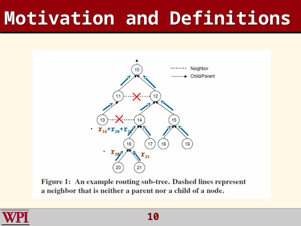
Motivation and DefinitionsMotivation and Definitions
r20 r21
r16+r20+r21
11
Motivation and DefinitionsMotivation and Definitions
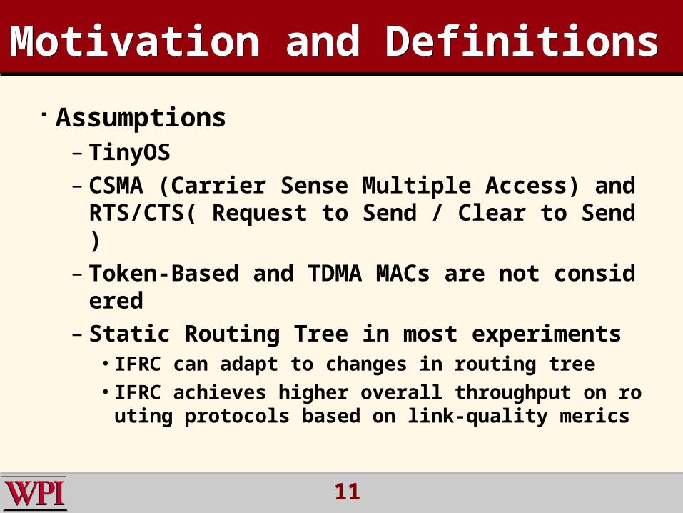
Assumptions– TinyOS– CSMA (Carrier Sense Multiple Access) and
RTS/CTS( Request to Send / Clear to Send)– Token-Based and TDMA MACs are not con
sidered– Static Routing Tree in most experiments• IFRC can adapt to changes in routing tree• IFRC achieves higher overall throughput on ro
uting protocols based on link-quality merics
12
Motivation and DefinitionsMotivation and Definitions
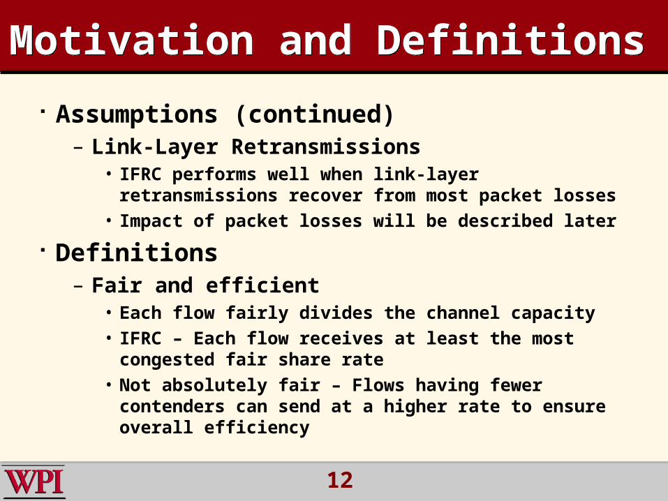
Assumptions (continued)– Link-Layer Retransmissions
• IFRC performs well when link-layer retransmissions recover from most packet losses
• Impact of packet losses will be described later
Definitions– Fair and efficient
• Each flow fairly divides the channel capacity• IFRC – Each flow receives at least the most congested
fair share rate• Not absolutely fair – Flows having fewer contenders can
send at a higher rate to ensure overall efficiency
13
Motivation and DefinitionsMotivation and Definitions
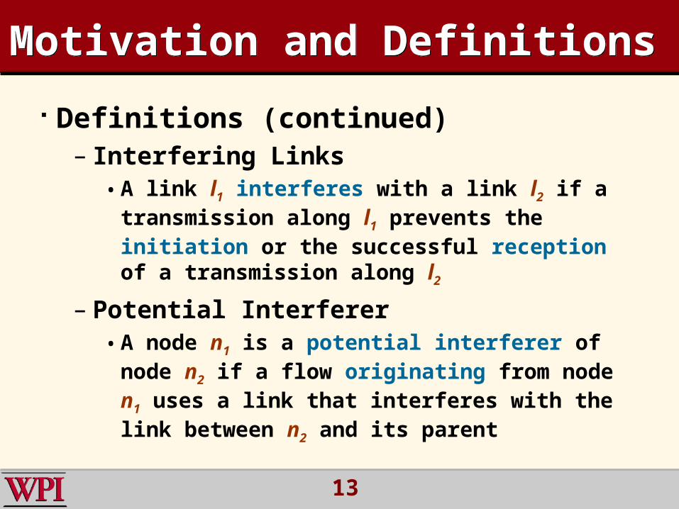
Definitions (continued)– Interfering Links• A link l1 interferes with a link l2 if a transmission
along l1 prevents the initiation or the successful reception of a transmission along l2
– Potential Interferer• A node n1 is a potential interferer of node n2 if a
flow originating from node n1 uses a link that interferes with the link between n2 and its parent
14
Motivation and DefinitionsMotivation and Definitions
15
Motivation and DefinitionsMotivation and Definitions
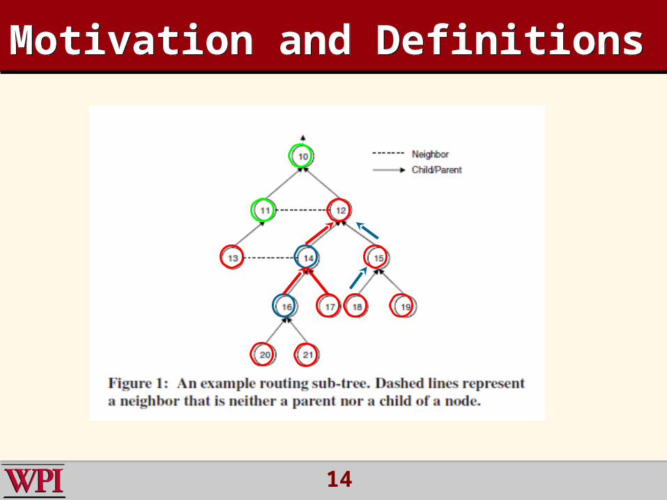
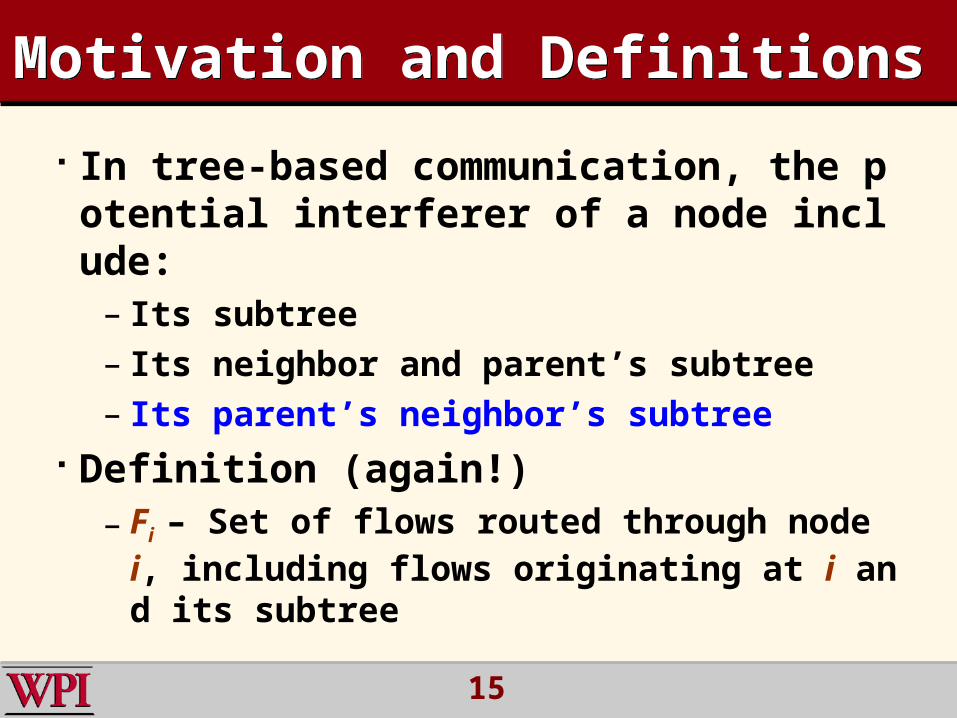
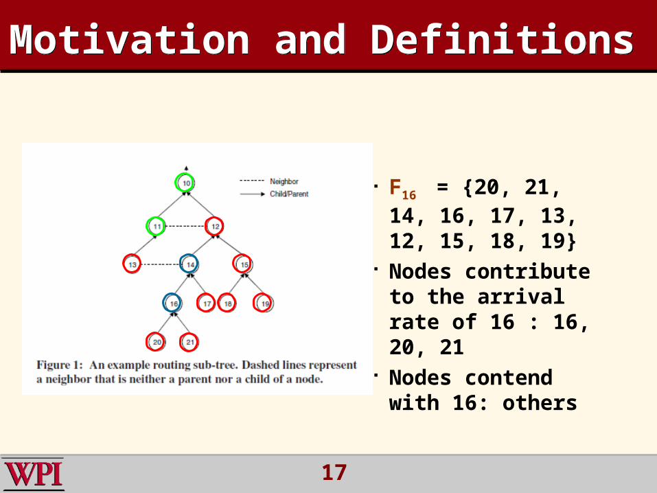
In tree-based communication, the potential interferer of a node include:– Its subtree– Its neighbor and parent’s subtree– Its parent’s neighbor’s subtree
Definition (again!)– Fi – Set of flows routed through node i, incl
uding flows originating at i and its subtree

16
Motivation and DefinitionsMotivation and Definitions
Definition (continued)– B : Nominal total bandwidth
– Fi = Fi + Fj , j is either a neighbor of i, or a neighbor of i’s parent ( set of all potential interferers)
– fl,i : the assigned rate of each flow in Fi
– fl : minimum of all fl,i
17
Motivation and DefinitionsMotivation and Definitions
F16 = {20, 21, 14, 16, 17, 13, 12, 15, 18, 19}
Nodes contribute to the arrival rate of 16 : 16, 20, 21
Nodes contend with 16: others
18
OutlineOutline
Introduction Related Work Motivation and Definitions
IFRC Design Parameter Selection In IFRC Evaluation Conclusions
19
IFRC DesignIFRC Design
Main Task– Congestion Detection– Signaling– Rate Adaptation
Congestion Detection– Channel Utilization– Queue size– With a MAC with carrier-sense, backoffs and retra
nsmission, overloaded traffic will increase the queue size. Therefore, we simply use queue size to indicate congestion.
20
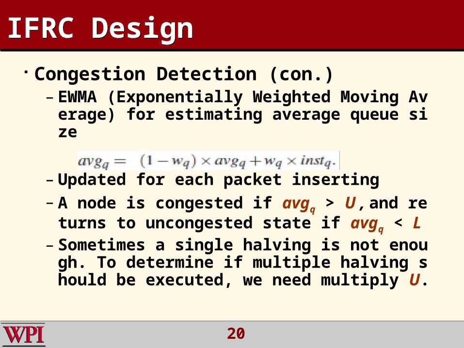
Congestion Detection (con.)– EWMA (Exponentially Weighted Moving Av
erage) for estimating average queue size
– Updated for each packet inserting– A node is congested if avgq > U , and return
s to uncongested state if avgq < L– Sometimes a single halving is not enough.
To determine if multiple halving should be executed, we need multiply U.
IFRC DesignIFRC Design
21
IFRC DesignIFRC Design
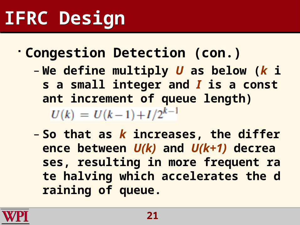
Congestion Detection (con.)–We define multiply U as below (k is a small
integer and I is a constant increment of queue length)
– So that as k increases, the difference between U(k) and U(k+1) decreases, resulting in more frequent rate halving which accelerates the draining of queue.
22
IFRC DesignIFRC Design
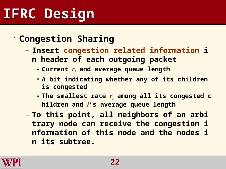
Congestion Sharing– Insert congestion related information in header of
each outgoing packet• Current ri and average queue length
• A bit indicating whether any of its children is congested
• The smallest rate rl among all its congested children and l’s average queue length
– To this point, all neighbors of an arbitrary node can receive the congestion information of this node and the nodes in its subtree.
23
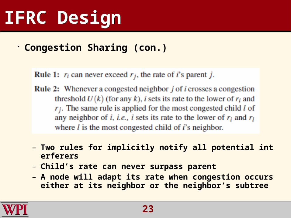
IFRC DesignIFRC Design Congestion Sharing (con.)
– Two rules for implicitly notify all potential interferers– Child’s rate can never surpass parent– A node will adapt its rate when congestion occurs either at i
ts neighbor or the neighbor’s subtree

24
IFRC DesignIFRC Design
Rate Adaptation– Average value of ri is not the max rate by which i g
enerate traffic– At the beginning, a node starts its sending rate at
rinit and add Φ to its rates every 1/ ri seconds.
– The node continues to increase the rate until itself congested or the two rules satisfied; Then it adapts the rate accordingly.
– After the adaptation, the node increases its ri by δ/ri every 1/ri seconds.
25
IFRC DesignIFRC Design
Base Station Behavior– Sets the initial rate rb to the nominal rate of
the channel and do not increases it– If any of its children is congested, decreas
es its rate, and broadcasts it twice
– After each adaptation, increments rb by δ/rb every 1/ rb seconds. As the station itself has no data to send, it broadcasts its rate after at least m packet have been received from the fastest child.
26
IFRC DesignIFRC Design
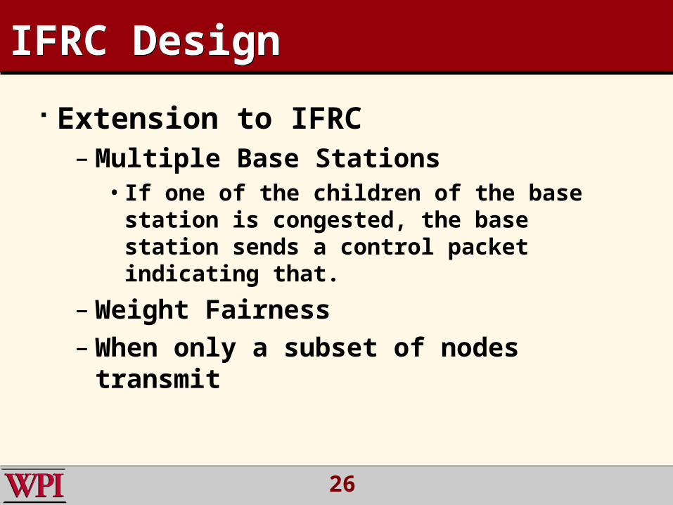
Extension to IFRC–Multiple Base Stations• If one of the children of the base station is
congested, the base station sends a control packet indicating that.
–Weight Fairness–When only a subset of nodes transmit
27
IFRC DesignIFRC Design
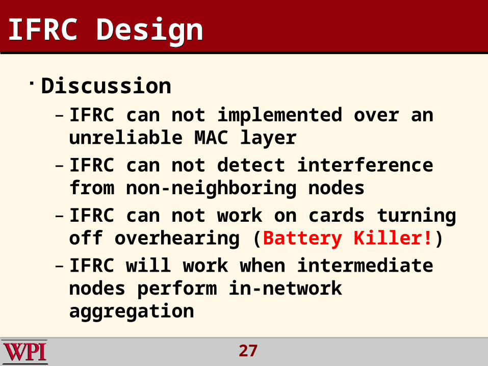
Discussion– IFRC can not implemented over an
unreliable MAC layer– IFRC can not detect interference from non-
neighboring nodes– IFRC can not work on cards turning off
overhearing (Battery Killer!)– IFRC will work when intermediate nodes
perform in-network aggregation
28
OutlineOutline
Introduction Related Work Motivation and Definitions IFRC Design
Parameter Selection In IFRC Evaluation Conclusions

29
Parameter Selection In IFRCParameter Selection In IFRC
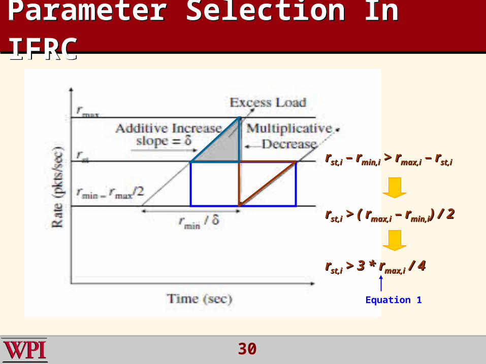
Intensity in AIMD– Each node i increases its rate ri by δ/ri every 1/ri s
econds.
– Namely, it follows a linear curve with slope δ. – For efficiency, δ should be as large as possible. H
owever, for stability δ should be kept not too large. So, our task is to find its upper bound in terms of maintaining the stability
30
Parameter Selection In IFRCParameter Selection In IFRC
rrst,ist,i – r – rmin,imin,i > r > rmax,imax,i – r – rst,ist,i
rrst,ist,i > ( r > ( rmax,imax,i – r – rmin,imin,i) / 2) / 2
rrst,ist,i > 3 * r > 3 * rmax,imax,i / 4 / 4
Equation 1
31
Parameter Selection In IFRCParameter Selection In IFRC
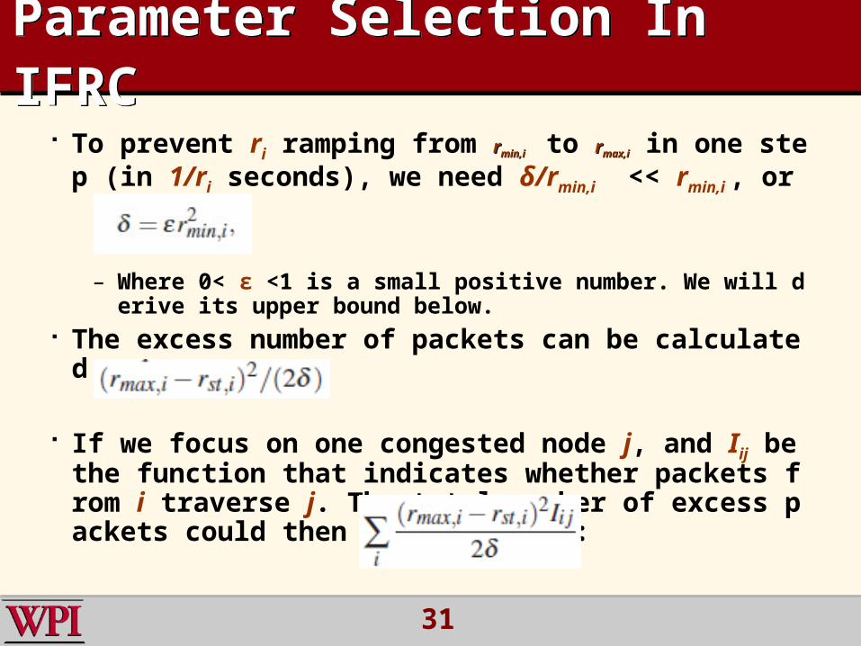
To prevent ri ramping from rrmin,imin,i to rrmax,imax,i in one step (in 1/r
i seconds), we need δ/rmin,i << rmin,i , or
– Where 0< ε <1 is a small positive number. We will derive its upper bound below.
The excess number of packets can be calculated as
If we focus on one congested node j, and Iij be the function that indicates whether packets from i traverse j. The total number of excess packets could then be denoted as:

32
Parameter Selection In IFRCParameter Selection In IFRC
Taking the effect of contention into account, we substitute Iij with fij.
We need to tune the value of to validate the following two equations:
Equation 1, 2, 3 guarantee system stability and only one signal is sent for one node when congestion occurs, which mitigates the reduce of efficiency.
Equation 2 Equation 3

33
Parameter Selection In IFRCParameter Selection In IFRC
By substituting rst in Equation 2 using Equation 1 and let Fj = Σi fij, we get
rrstst =1.5 * r =1.5 * rminmin
(See the figure) As rst rises, the difference between the area of two triangles increase, thus the efficiency decreases.
As rst drops, the upper bound of εdrops, so we will get a smallerε.
34
Parameter Selection In IFRCParameter Selection In IFRC
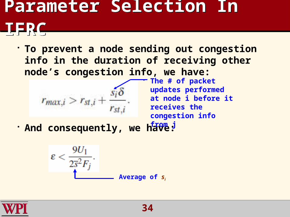
To prevent a node sending out congestion info in the duration of receiving other node’s congestion info, we have:
And consequently, we have:
The # of packet updates performed at node i before it receives the congestion info from j
Average of si
35
Parameter Selection In IFRCParameter Selection In IFRC
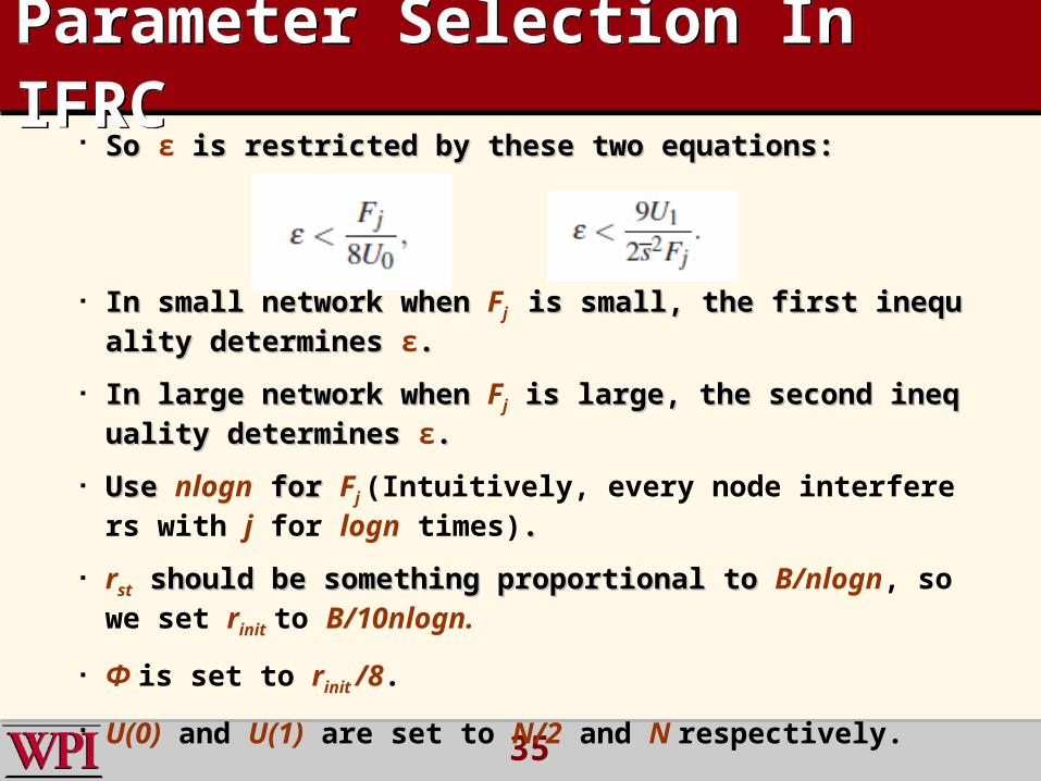
In small network when In small network when Fj is small, the first inequality determinis small, the first inequality determin
es es ε..
In large network when In large network when Fj is large, the second inequality deter is large, the second inequality deter
mines mines ε..
Use Use nlogn for for Fj (Intuitively, every node interferers with j for logn times). .
rst should be something proportional to should be something proportional to B/nlogn, so we set rinit to B/10nlogn.
Φ is set to rinit /8.
U(0) and U(1) are set to N/2 and N respectively.
So So ε is restricted by these two equations: is restricted by these two equations:
36
OutlineOutline
Introduction Related Work Motivation and Definitions IFRC Design Parameter Selection In IFRC
Evaluation Conclusions
37
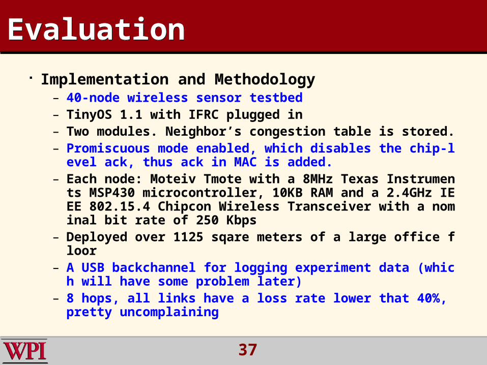
EvaluationEvaluation Implementation and Methodology
– 40-node wireless sensor testbed– TinyOS 1.1 with IFRC plugged in– Two modules. Neighbor’s congestion table is stored.– Promiscuous mode enabled, which disables the chip-level a
ck, thus ack in MAC is added.– Each node: Moteiv Tmote with a 8MHz Texas Instruments M
SP430 microcontroller, 10KB RAM and a 2.4GHz IEEE 802.15.4 Chipcon Wireless Transceiver with a nominal bit rate of 250 Kbps
– Deployed over 1125 sqare meters of a large office floor– A USB backchannel for logging experiment data (which will
have some problem later)– 8 hops, all links have a loss rate lower that 40%, pretty unco
mplaining
38
EvaluationEvaluation
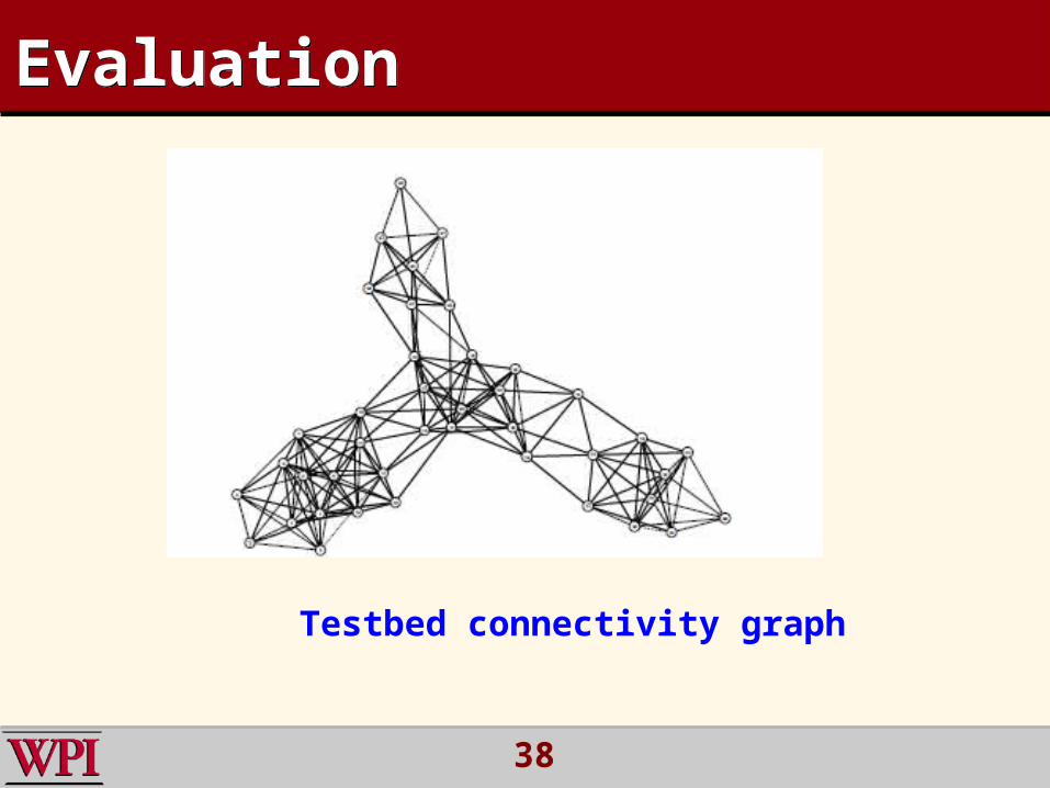
Testbed connectivity graph
39
EvaluationEvaluation
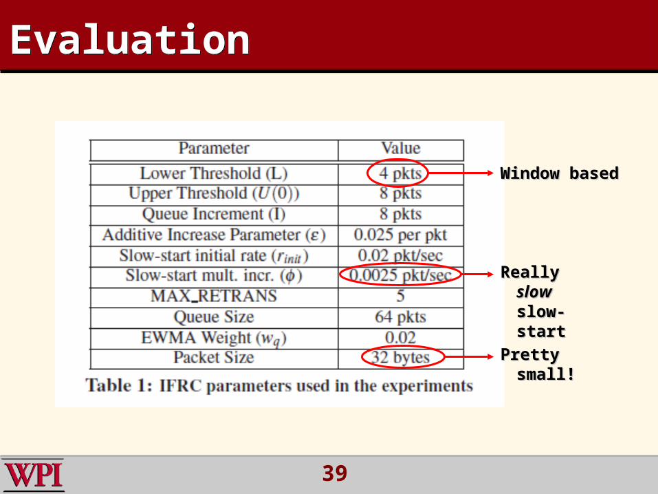
Window basedWindow based
Pretty small!Pretty small!
Really Really slow slow slow-startslow-start
40
EvaluationEvaluation
A fixed tree to maintain a same environment for all experiments (modifies MultiHopLQI)
A hour at least for each experiment Long experiments, run at usually late at
night or in early morning Every packet transmission, reception, a
nd every change in rate at each node (including base station, although no transmission) is recorded.
41
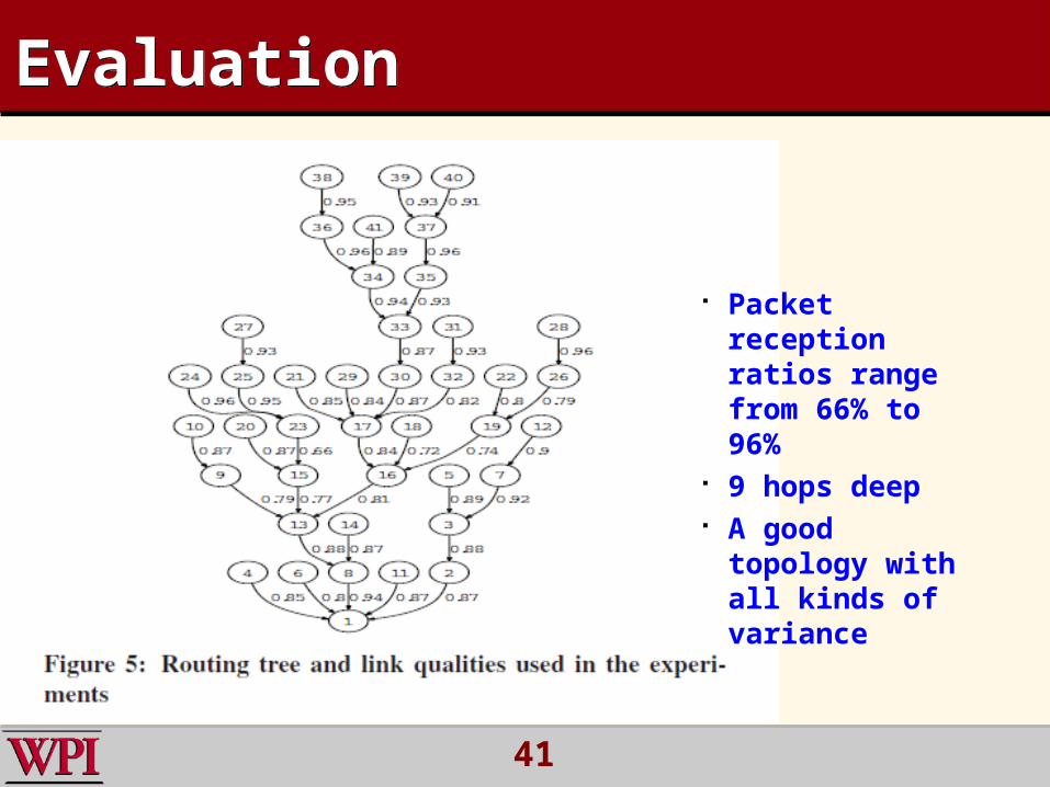
EvaluationEvaluation
Packet reception ratios range from 66% to 96%
9 hops deep A good topology
with all kinds of variance
42
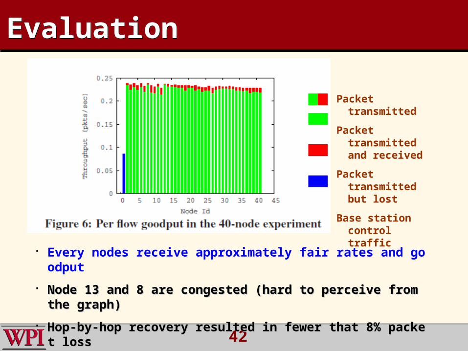
EvaluationEvaluation
Packet transmitted
Packet transmitted and received
Packet transmitted but lost
Base station control traffic
Every nodes receive approximately fair rates and goodput
Node 13 and 8 are congested (hard to perceive from the graph)Node 13 and 8 are congested (hard to perceive from the graph)
Hop-by-hop recovery resulted in fewer that 8% packet lossHop-by-hop recovery resulted in fewer that 8% packet loss
43
EvaluationEvaluation
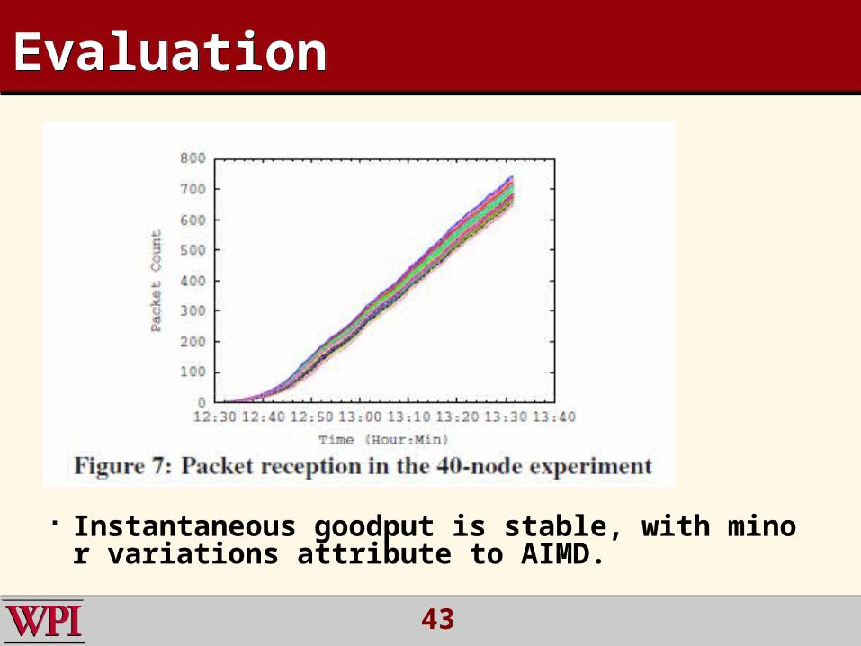
Instantaneous goodput is stable, with minor variations attribute to AIMD.
44
EvaluationEvaluation
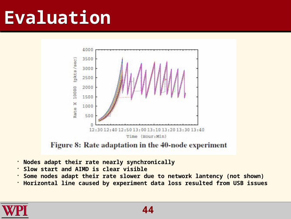
Nodes adapt their rate nearly synchronically Slow start and AIMD is clear visible Some nodes adapt their rate slower due to network lantency (not shown) Horizontal line caused by experiment data loss resulted from USB issues
45
EvaluationEvaluation
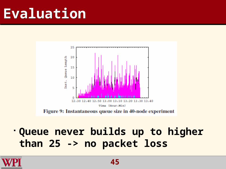
Queue never builds up to higher than 25 -> no packet loss
46
EvaluationEvaluation
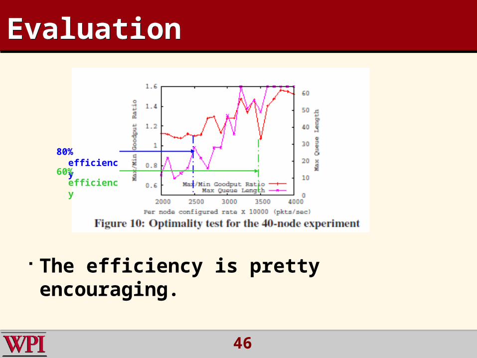
The efficiency is pretty encouraging.
80% efficiency
60% efficiency
47
EvaluationEvaluation
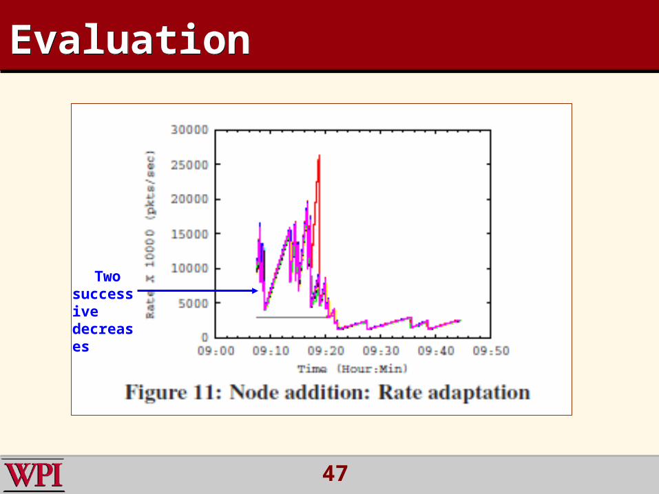
Two successive decreases
48
EvaluationEvaluation
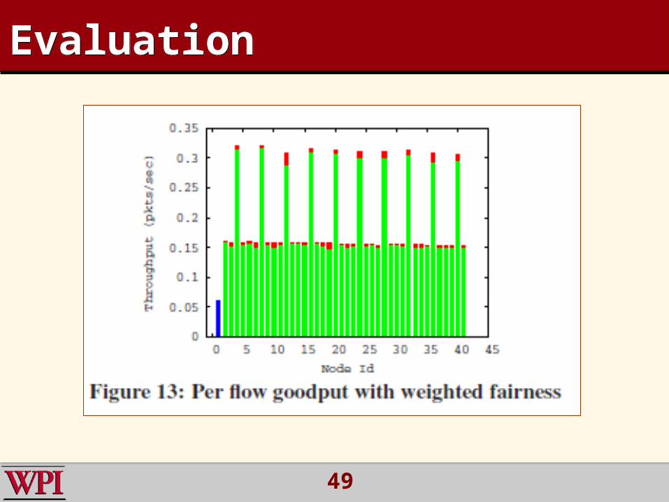
49
EvaluationEvaluation
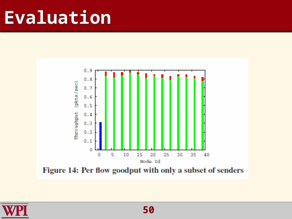
50
EvaluationEvaluation
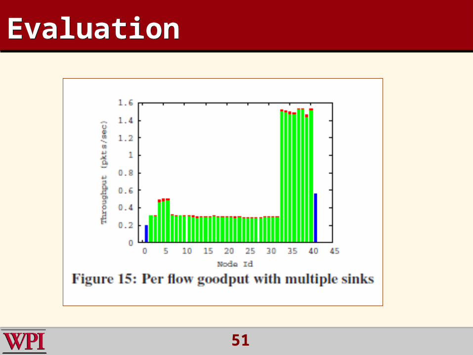
51
EvaluationEvaluation

52
EvaluationEvaluation
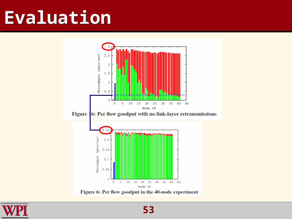
53
EvaluationEvaluation
54
OutlineOutline
Introduction Related Work Motivation and Definitions IFRC Design Parameter Selection In IFRC Evaluation
Conclusions
55
ConclusionsConclusions
Conclusion– IFRC is the first practical interference-aware rate
control mechanism for WSN– IFRC is fair– In terms of efficiency, IFRC is questionable
Future work– Implement reliability in IFRC– A more rigorous proof of the choice of IFRC
parameters– A complete analysis of the effects of other factors
on IFRC

56
Thank you!Thank you!