Embed Size (px)
Citation preview
1
Chapter 1
Introduction
Control Systems and Networks
Networked control systems (NCSs) are the collaboration of two engineering fields,
communication engineering (either wired or wireless) and control engineering.
Because most NCSs are done in a wired environment, understanding network protocols
such as Ethernet, token bus, token ring and CAN, is required to model the system’s
behavior.
The ISO (International Standard Organization) has set up a guideline for
computer networking called the open system interconnection (OSI). The OSI is divided
into seven layers: the physical layer, the data link layer, the network layer, the transport
layer, the session layer, the presentation layer and the application layer from the lowest to
the highest respectively. The IEEE 802 committee has issued standards for local area
networks (LANs): IEEE 802.3 (Ethernet), IEEE 802.4 (token bus) and IEEE 802.5 (token
ring). In LANs, the sublayer responsible for time critical/real time information is the
medium access control (MAC). Technically, the MAC sublayer is the bottom part of the
data link layer. It is responsible the assurance of the connection between nodes over the
network.
Ethernet (IEEE 802.3) uses the carrier sense multiple access with collision
detection (CSMA/CD) protocol to control its communication. The transmitting nodes
terminate their transmission after detected collisions. They wait for a random period and
try to send the frames again. The protocol is bandwidth efficient as justified in [8].
2
The token bus (IEEE 802.4) is physically connected in a linear or tree-shaped
manner. Logically, the connection between stations is considered as a ring, where each
station knows its two logical neighbors. However, in order to use the protocol, the worst-
case time delay must be known. Even though the physical connection is linear, it does not
mean that physically successive station will receive the token after the previous station is
done. The token is passed to the station’s logical neighbors.
When initialized, the hierarchy of stations is considered by the MAC sublayer by
their addresses, the station with the highest number is the beginner. The station with a
token may send frames during some amount of time and it has to pass the token on. The
token bus divides the data into four priority classes, 0, 2, 4 and 6. When a station gets a
token, data with priority 6 is sent first and priority 0 is the last with some measure to
guarantee the data with priority 0 gets some allocation.
The IEEE 802.5 (token ring) network has a special bit pattern, called the token,
available for a station to acquire when the network is idle. The token is removed from the
network when a station decides to make a transmission. The token is regenerated after
the transmitting station finishes its transmission. An implication of the token ring design
is that the ring itself must have a sufficient time delay to allow a complete token to allow
a token to circulate completely when all stations are idle.
Another common protocol in today’s business is the controller area network
(CAN). CAN is a serial communication protocol that was developed to support
applications in the automotive industry. The MAC sublayer in the protocol is carrier
sense multiple access with arbitration on message priority (CSMA/AMP). The protocol
uses a multicast technique, i.e. a station transmits a message and other stations decide to
3
accept or ignore the message depending on the configuration of a masking filter. For
collision protection, each message has a specific priority that is used to arbitrate access to
the bus where logic zero is dominant over logic one. This conflict is resolved during
transmission at the bit level of the arbitration field. A common-use CAN-based system in
device-level manufacturing is the DeviceNet. It uses standard CAN with an additional
application and physical layer specification. [4]
Categorized by the MAC algorithms, the protocols fall into two categories, ones
that produce constant transmission periods and those that create time-varying
transmission periods. The algorithms used in the IEEE 802.4 standard and the IEEE
802.5 standard yield constant transmission periods, whereas the IEEE 802.3 standard and
CAN produce time-varying transmission periods. Bounds for the transmission period will
be needed to guarantee stability of NCSs. This topic was studied in [7], [9], &[10].
Also, based on the MAC algorithms, the delay between transmissions (networked-
induced delay) is divided into two groups, deterministic and non-deterministic. If the
MAC sublayer of a protocol accesses channel using the random back-off CSMA/CD in
the Ethernet, for example, the delay from the protocol will be random. On the other hand,
the scheduling protocols (the IEEE 802.4 standard and the IEEE 802.5 standard) will give
deterministic delay.
Other concerns for stability of NCSs are length of transmitted packets and packet
dropping. The underlying protocol of the MAC sublayer in the network is the key to
controlling the length of packets to be transmitted. In Ethernet, for example, the data field
of the protocol is 1,500 bytes, so the size of transmitted packets is unlikely to affect real-
time feedback signals which are only a few bytes each. The information can even be
4
lumped and transmitted in one packet. On the other hand, the data field in the DeviceNet
is only 8 bytes. The sensor data must be divided and transmitted in several packets.
Packet dropping is often an inevitable event in network data transmission despite
the provisions network protocols. In real-time feedback control, it might be advantageous
to drop an old control signal and implement a new one. These issues were studied in [11].
Throughout the simulations within, we assume single packet transmission with a
fixed transmission period from a digital controller equipped with an estimator. The study
of delay estimation in feedback control systems in network environments is the focus. For
networks using scheduling protocols, we propose static delay estimation to compensate
the system. For random access protocols, the network-induced delay is non-deterministic.
The static delay compensation is not effective in these environments. Another approach,
called dynamic delay compensation, is proposed for this scenario. The study is elaborated
in Chapter 3.
Thesis Organization
This thesis is organized as follows. Some background material and related
mathematical analysis of NCSs are reviewed in Chapter 2. This chapter also includes
network delay modeling of some NCSs (CAN and Ethernet). However, the main
contributions to the NCSs are in Chapter 3. This chapter explains about the importance
of the compensation of immeasurable delay, e.g. τca, and how it affects systems if it is not
compensated for. We summarize and conclude our study in Chapter 4.
5
Chapter2
Background
State-Space Model for Systems with Delay
Delay Less Than One Sampling Period†
Consider the linear state equations with input delayed by λ :
),()()( λ−+= tutt BAxx& (2.1)
.Hx=y (2.2)
The general solution to the equation is
τλττ duetett
t
ttt )()()(0
0 )(0
)( −+= ∫ −− Bxx AA& . (2.3)
By sampling the system with sampling period h the solution for the state is
τλττ duekhehkhhkh
kh
hkhh )()()( )()( −+=+ ∫+
−+ Bxx AA . (2.4)
where we assume 0 < λ < T.
While the signal u(t) is assumed piecewise constant over the sampling period
interval, u(t-λ) is not piecewise constant over the sampling period interval. The delayed
signal will change once during sampling period. The modified solution to the equation is
)()()()( )()()( khudehkhudekhehkhhkh
kh
hkhkh
kh
hkhh ττλ
τλ
τ BBxx AAA ∫∫+
+
−++
−+ +−+=+ . (2.5)
A discrete-time state-space model of the system is given by
),()(
)(
)(
)( 01 khuhkhu
khkhu
hkh
Γ+
−
ΓΦ=
+I
x
00
x (2.6)
_________________________ † See [1] for details
6
where
).(
),(
,
)(1
)(0
hkhude
khude
e
kh
kh
hkh
hkh
kh
hkh
h
−=Γ
=Γ
=Φ
∫
∫+
−+
+
+
−+
τ
τ
λτ
λ
τ
B
B
A
A
A
Longer Time Delay‡
If the time delay, λ, is longer than the sampling period, h. The analysis in 2.2.1
needs a little adaptation. Decompose λ into multiples of T:
λλ ′+−= hd )1( 0 < λ’ ≤ h, (2.7)
where d is an integer. The analysis is modified to
)())1(()()( 10 dhkhuhdkhukhhkh −Γ+−−Γ+Φ=+ xx , (2.8)
with the same Φ, Γ0 and Γ1 as in section 2.1.1.
The corresponding state-space description is
)(
0
0
0
)(
)2(
)(
)(
0000
000
000
00
)()(
))1((
)( 01
khu
hkhuhkhu
dhkhukh
khuhkhu
hdkhuhkh
+
−−
−
ΓΓΦ
=
−
−−+
I
x
I
Ix
MM
L
L
MOMMM
L
M . (2.9)
_________________________ ‡ See [3] for details
7
Compensation for Network-Induced Delay
In this section we review the compensation discussed in [10], [11]. The
compensation of NCSs is considered for sensor-to-controller delay, τsc, only. Feedback
systems are categorized to full-state feedback or output feedback systems. With full-state
feedback, the estimator compensates τsc. In the output feedback system, the estimator has
to do both compensation and the estimate state of the system. These methods are
compromising as far as delays are measurable. We use these approaches as our basic idea
for developing the compensation for both of measurable and immeasurable delays.
Full-State Feedback
Let a system be described as in (2.1) and (2.2), λ < h. For every plant output, the
data is time-stamped by the sensor in order to acquire the information about current time
delay, τsc,k. Sensor information reaches the estimator at time ksckh ,τ+ . By assuming there
is no measurement noise and all states are measured, the plant information at that time is
dssuekhekhkhksc
kscksc
khkh
kscksc )()()()(,
,,
0
)()(,, Bxxx
AA ∫+
−+=+=+τ
ττττ , (2.10)
where )( .ksckh τ+x is the estimated state at time ksckh ,τ+ .
Applying the state feedback control law to the system
)()( ,, kscksc khkhu ττ +⋅−=+ xK , (2.11)
)()(~
))1(( ,1, ksckksc khhk τδτ +⋅⋅Φ=++ + xx . (2.12)
where
kscksck h ,1, ττδ −−= + ,
K⋅Γ+Φ=Φ )()()(~
kkk δδδ ,
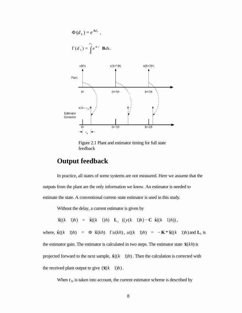
8
kekδδ A=Φ )( ,
.)(0
dsek
sk ∫ ⋅=Γ
δ
δ BA
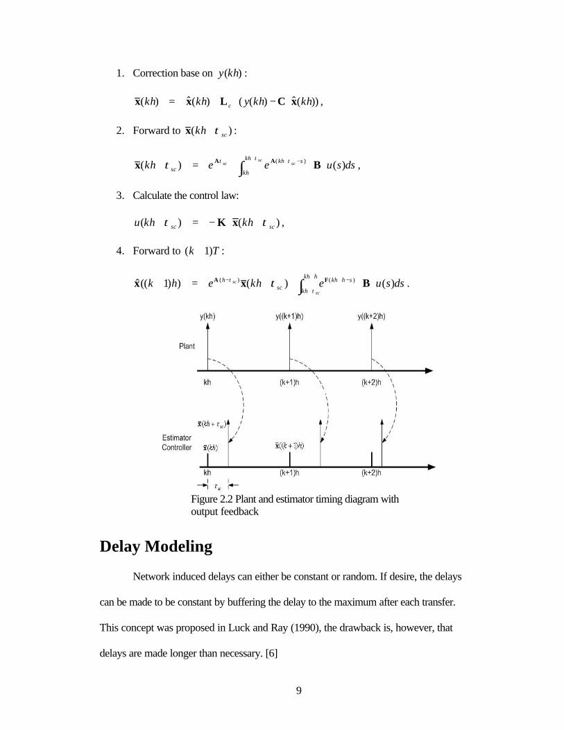
Figure 2.1 Plant and estimator timing for full state feedback
Output feedback
In practice, all states of some systems are not measured. Here we assume that the
outputs from the plant are the only information we know. An estimator is needed to
estimate the state. A conventional current-state estimator is used in this study.
Without the delay, a current estimator is given by
)))1((ˆ))1((())1((ˆ))1(( hkhkyhkhk c +⋅−+⋅++=+ xCLxx ,
where, )()())1((ˆ khukhhk Γ+⋅Φ=+ xx , ))1((*))1(( hkhku +−=+ xK and Lc is
the estimator gain. The estimator is calculated in two steps. The estimator state )(khx is
projected forward to the next sample, ))1((ˆ hk +x . Then the calculation is corrected with
the received plant output to give ))1(( hk +x .
When τsc is taken into account, the current estimator scheme is described by
9
1. Correction base on )(khy :
))(ˆ)(()(ˆ)( khkhykhkh c xCLxx ⋅−⋅+= ,
2. Forward to )( sckh τ+x :
dssueekh scscsc
kh
kh
skhsc )()( )( ⋅⋅+=+ ∫
+ −+τ τττ Bx AA ,
3. Calculate the control law:
)()( scsc khkhu ττ +⋅−=+ xK ,
4. Forward to Tk )1( + :
dssuekhehkhkh
kh
shkhsc
h
sc
sc )()())1((ˆ )()( ⋅⋅++=+ ∫+
+
−+−
τ
τ τ Bxx FA .
Figure 2.2 Plant and estimator timing diagram with output feedback
Delay Modeling
Network induced delays can either be constant or random. If desire, the delays
can be made to be constant by buffering the delay to the maximum after each transfer.
This concept was proposed in Luck and Ray (1990), the drawback is, however, that
delays are made longer than necessary. [6]
10
Constant Delay
In CAN-base networks, data (packet) contention for network channel usage is low
or non-existent since its topology is similar to a token bus network [4]. It is safe to say,
therefore, that there is only one packet in the network channel from one channel. This
includes periodically sent packets with idle network channels at the time of transmission.
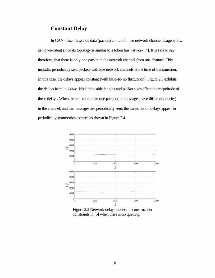
In this case, the delays appear constant (with little-to-no fluctuation). Figure 2.3 exhibits
the delays from this case. Note that cable lengths and packet sizes affect the magnitude of
these delays. When there is more than one packet (the messages have different priority)
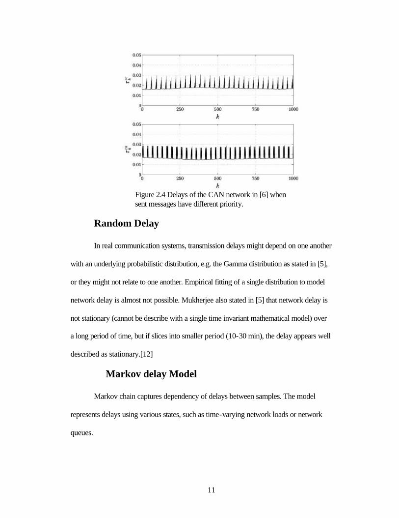
in the channel, and the messages are periodically sent, the transmission delays appear in
periodically symmetrical pattern as shown in Figure 2.4.
Figure 2.3 Network delays under the construction constraints in [6] when there is no queuing.
11
Figure 2.4 Delays of the CAN network in [6] when sent messages have different priority.
Random Delay
In real communication systems, transmission delays might depend on one another
with an underlying probabilistic distribution, e.g. the Gamma distribution as stated in [5],
or they might not relate to one another. Empirical fitting of a single distribution to model
network delay is almost not possible. Mukherjee also stated in [5] that network delay is
not stationary (cannot be describe with a single time invariant mathematical model) over
a long period of time, but if slices into smaller period (10-30 min), the delay appears well
described as stationary.[12]
Markov delay Model
Markov chain captures dependency of delays between samples. The model
represents delays using various states, such as time-varying network loads or network
queues.
12
Markov Chain
A finite Markov chain is a Markov process that takes values {rk} in a finite set S =
{1,2 ,3…,s}, with transition probabilities
ijkk qirjrP ===+ )|( 1 , (2.13)
The transition probabilities, qij, fulfill qij ≥ 0 for all Sji ∈, , and
11
=∑=
s
jijq . (2.14)
The Markov State probability distribution is
)]()()([)( 21 kkkk sππππ K= , (2.15)
where πi(k) is the probability that the Markov chain state at time k is i. The probability
distribution for rk is given by
Q)()1( kk ππ =+ , (2.16)
where the initial state probability
0)0( ππ = . (2.17)
A Markov chain is said to be regular if the transition matrix Q is a primitive
matrix, i.e. all its elements are strictly positive. That a Markov chain is regular means that
all states will be possible to reach in the future, there are no “dead ends” in the Markov
chain.
If a Markov chain is primitive the stationary probability distribution
)(lim kk ππ ∞→∞ = is given uniquely satisfies
Q∞∞ = ππ , (2.19)
where ∞π is a probability distribution.
13
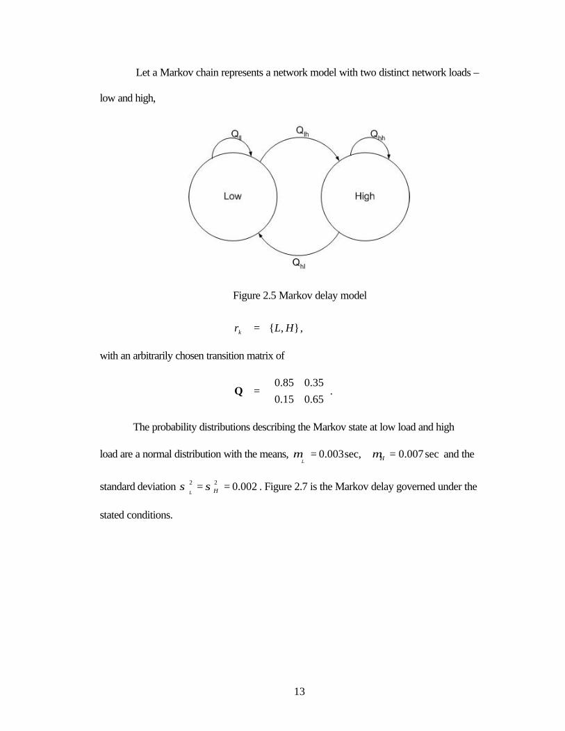
Let a Markov chain represents a network model with two distinct network loads –
low and high,
Figure 2.5 Markov delay model
},{ HLrk = ,
with an arbitrarily chosen transition matrix of
=
65.015.0
35.085.0Q .
The probability distributions describing the Markov state at low load and high
load are a normal distribution with the means, sec007.0sec,003.0 == HLµµ and the
standard deviation 002.022 == HLσσ . Figure 2.7 is the Markov delay governed under the
stated conditions.
14
0 0.001 0.002 0.003 0.004 0.005 0.006 0.007 0.008 0.009 0.010
2
4
6
8
10
Delay (sec)
Freq
uenc
y
0 0.001 0.002 0.003 0.004 0.005 0.006 0.007 0.008 0.009 0.010
2
4
6
8
10
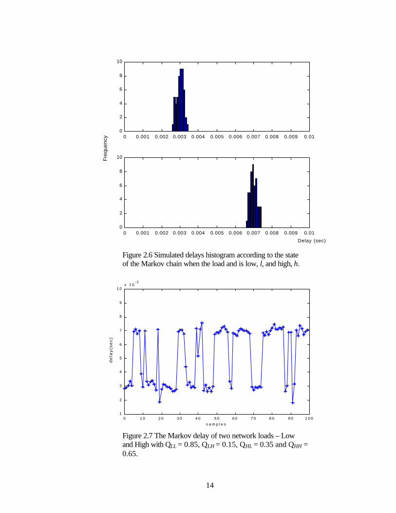
Figure 2.6 Simulated delays histogram according to the state of the Markov chain when the load and is low, l, and high, h.
0 1 0 2 0 3 0 4 0 5 0 6 0 7 0 8 0 9 0 1 0 01
2
3
4
5
6
7
8
9
1 0x 1 0
-3
s a m p l e s
de
lay(
sec)
Figure 2.7 The Markov delay of two network loads – Low and High with QLL = 0.85, QLH = 0.15, QHL = 0.35 and QHH = 0.65.
15
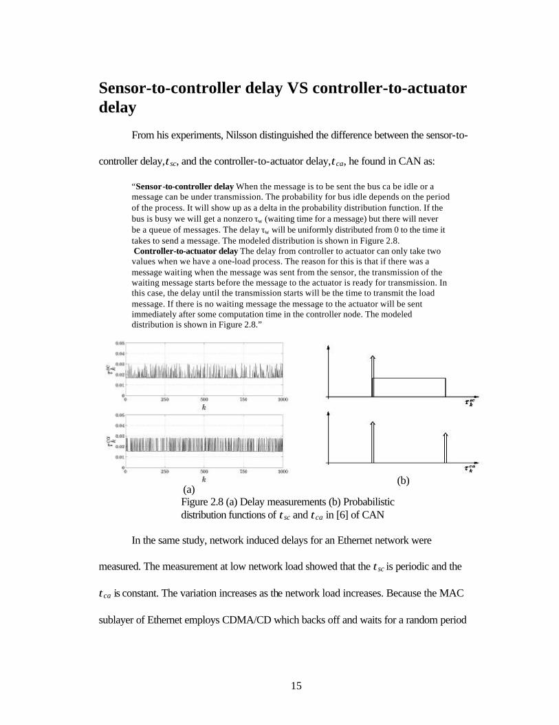
Sensor-to-controller delay VS controller-to-actuator delay From his experiments, Nilsson distinguished the difference between the sensor-to-
controller delay,τsc, and the controller-to-actuator delay,τca, he found in CAN as:
“Sensor-to-controller delay When the message is to be sent the bus ca be idle or a message can be under transmission. The probability for bus idle depends on the period of the process. It will show up as a delta in the probability distribution function. If the bus is busy we will get a nonzero τw (waiting time for a message) but there will never be a queue of messages. The delay τw will be uniformly distributed from 0 to the time it takes to send a message. The modeled distribution is shown in Figure 2.8. Controller-to-actuator delay The delay from controller to actuator can only take two values when we have a one-load process. The reason for this is that if there was a message waiting when the message was sent from the sensor, the transmission of the waiting message starts before the message to the actuator is ready for transmission. In this case, the delay until the transmission starts will be the time to transmit the load message. If there is no waiting message the message to the actuator will be sent immediately after some computation time in the controller node. The modeled distribution is shown in Figure 2.8.”
(a)
(b)
Figure 2.8 (a) Delay measurements (b) Probabilistic distribution functions of τsc and τca in [6] of CAN
In the same study, network induced delays for an Ethernet network were
measured. The measurement at low network load showed that the τsc is periodic and the
τca is constant. The variation increases as the network load increases. Because the MAC
sublayer of Ethernet employs CDMA/CD which backs off and waits for a random period
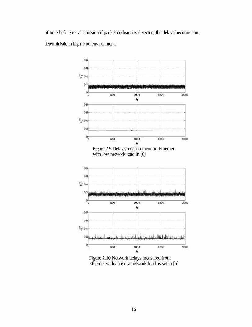
16
of time before retransmission if packet collision is detected, the delays become non-
deterministic in high-load environment.
Figure 2.9 Delays measurement on Ethernet with low network load in [6]
Figure 2.10 Network delays measured from Ethernet with an extra network load as set in [6]
17
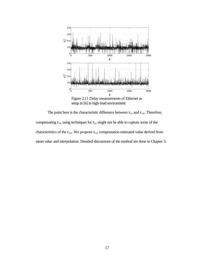
Figure 2.11 Delay measurements of Ethernet as setup in [6] in high-load environment
The point here is the characteristic difference between τsc and τca. Therefore,
compensating τca using techniques for τsc might not be able to capture some of the
characteristics of the τca. We propose τca compensation estimated value derived from
mean value and interpolation. Detailed discussions of the method are done in Chapter 3.
18
Chapter3
Network Induced Delays and Compensation
Introduction
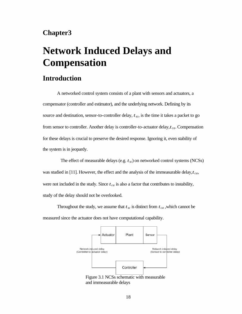
A networked control system consists of a plant with sensors and actuators, a
compensator (controller and estimator), and the underlying network. Defining by its
source and destination, sensor-to-controller delay, τsc, is the time it takes a packet to go
from sensor to controller. Another delay is controller-to-actuator delay,τca. Compensation
for these delays is crucial to preserve the desired response. Ignoring it, even stability of
the system is in jeopardy.
The effect of measurable delays (e.g. τsc) on networked control systems (NCSs)
was studied in [11]. However, the effect and the analysis of the immeasurable delay,τca,
were not included in the study. Since τca is also a factor that contributes to instability,
study of the delay should not be overlooked.
Throughout the study, we assume that τsc is distinct from τca ,which cannot be
measured since the actuator does not have computational capability.
Figure 3.1 NCSs schematic with measurable and immeasurable delays
19
Compensation of ττca
Let a system be described by
)()()( casctutt ττ −−⋅+= BxAx && . (3.1)
The system is sampled and integrated over one sampling period,
∫+ −+ −−⋅+=+
hkh
kh cascshkhh dssuekhehkh )()()( )( ττBxx AA . (3.2)
Because the control signal, u(kh), is piecewise constant over sampling periods, the
delayed version of it will be piecewise constant over a similarly delayed period.
.)(
)(
)()()(
)(
)(
)(
∫
∫∫
+
++
−+
++
+
−+
+ −+
⋅+
−⋅+
−⋅+=+
hkh
kh
shkh
kh
kh
shkh
kh
kh
shkhh
casc
casc
sc
sc
khudse
hkhudse
hkhudsekhehkh
ττ
ττ
τ
τ
B
B
Bxx
A
A
AA
(3.3)
Interpretation of these equations is not as complicated as the equations themselves
may look. After a sampling instant, sampled data travel through network to the
compensator (Figure 3.2). The compensator calculates appropriate control signal, u(kh),
with the factor of the τsc in consideration. The control signal, however, cannot be put to
use immediately because of the τca. The previous control signal, u(kh-h), therefore, is
used during the sampling period before the control signal, u(kh), reaches the actuators.
Note that computational delays were absorbed into τsc (if measurable) or τca (if
immeasurable).
20
Figure 3.2 Timing diagram of a delayed system
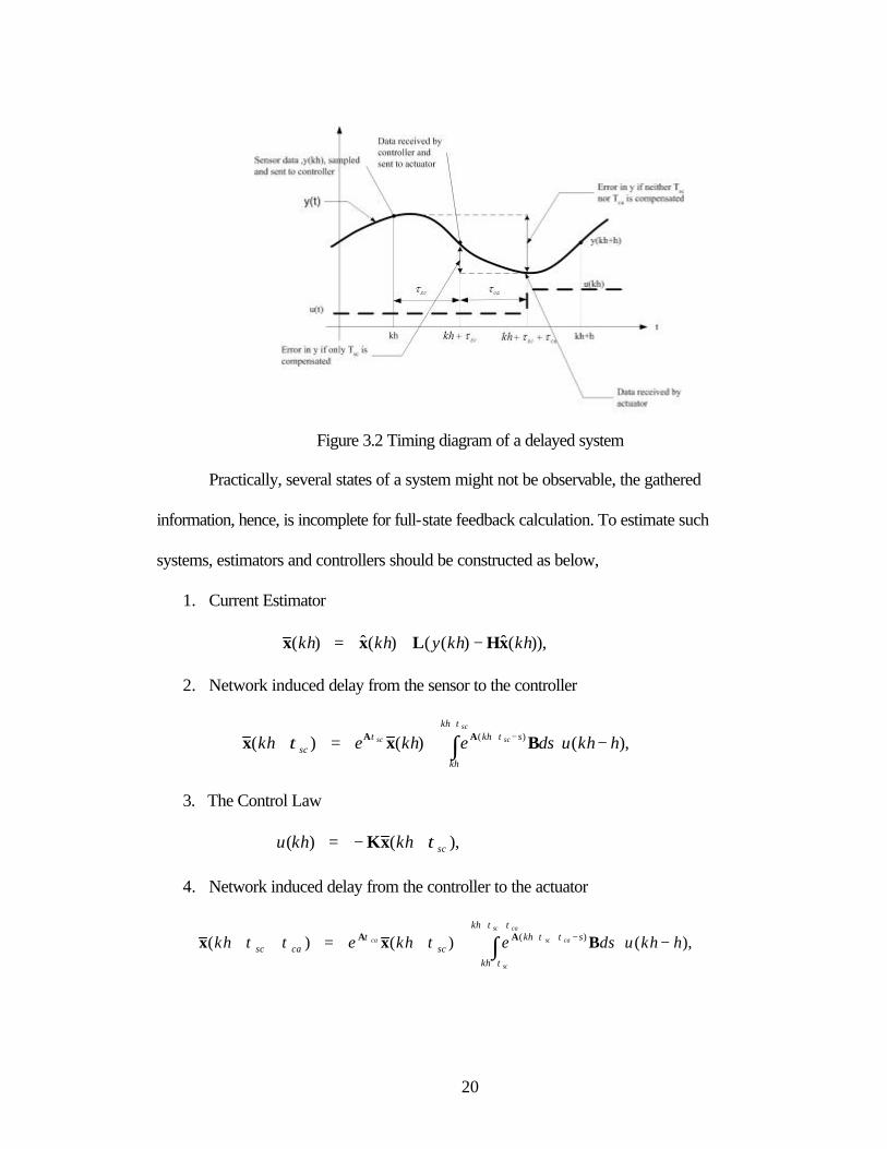
Practically, several states of a system might not be observable, the gathered
information, hence, is incomplete for full-state feedback calculation. To estimate such
systems, estimators and controllers should be constructed as below,
1. Current Estimator
)),(ˆ)(()(ˆ)( khkhykhkh xHLxx −+=
2. Network induced delay from the sensor to the controller
∫+
−+ −⋅+=+sc
scsc
kh
kh
skhsc hkhudsekhekh
ττττ ),()()( )( Bxx AA
3. The Control Law
),()( sckhkhu τ+−= xK
4. Network induced delay from the controller to the actuator
∫++
+
−++ −⋅++=++casc
sc
cascca
kh
kh
skhsccasc hkhudsekhekh
ττ
τ
τττ τττ ),()()( )( Bxx AA
21
5. Forward to )(ˆ hkh+x
∫+
++
−+−− ⋅+++=+hkh
kh
shkhcasc
h
casc
casc khudsekhehkhττ
ττ ττ ).()()(ˆ )()( Bxx AA
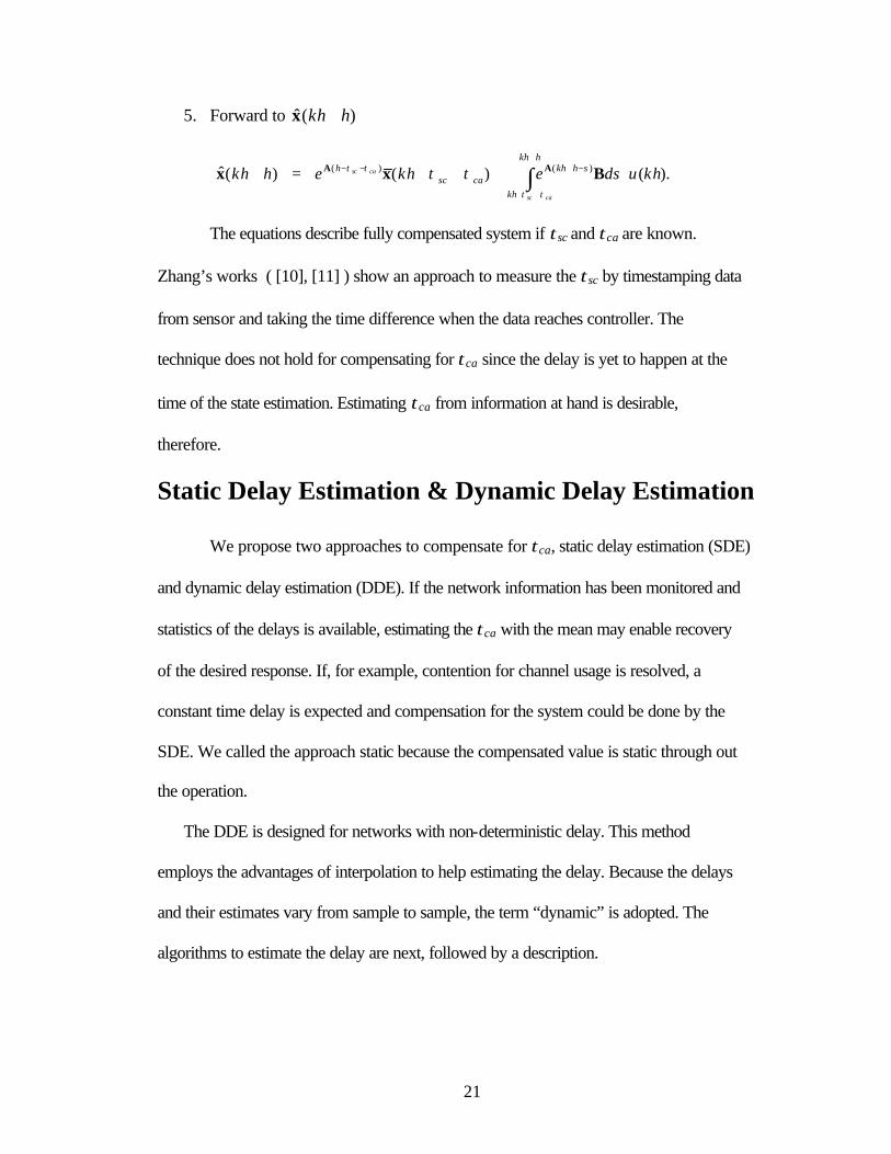
The equations describe fully compensated system if τsc and τca are known.
Zhang’s works ( [10], [11] ) show an approach to measure the τsc by timestamping data
from sensor and taking the time difference when the data reaches controller. The
technique does not hold for compensating for τca since the delay is yet to happen at the
time of the state estimation. Estimating τca from information at hand is desirable,
therefore.
Static Delay Estimation & Dynamic Delay Estimation
We propose two approaches to compensate for τca, static delay estimation (SDE)
and dynamic delay estimation (DDE). If the network information has been monitored and
statistics of the delays is available, estimating the τca with the mean may enable recovery
of the desired response. If, for example, contention for channel usage is resolved, a
constant time delay is expected and compensation for the system could be done by the
SDE. We called the approach static because the compensated value is static through out
the operation.
The DDE is designed for networks with non-deterministic delay. This method
employs the advantages of interpolation to help estimating the delay. Because the delays
and their estimates vary from sample to sample, the term “dynamic” is adopted. The
algorithms to estimate the delay are next, followed by a description.
22
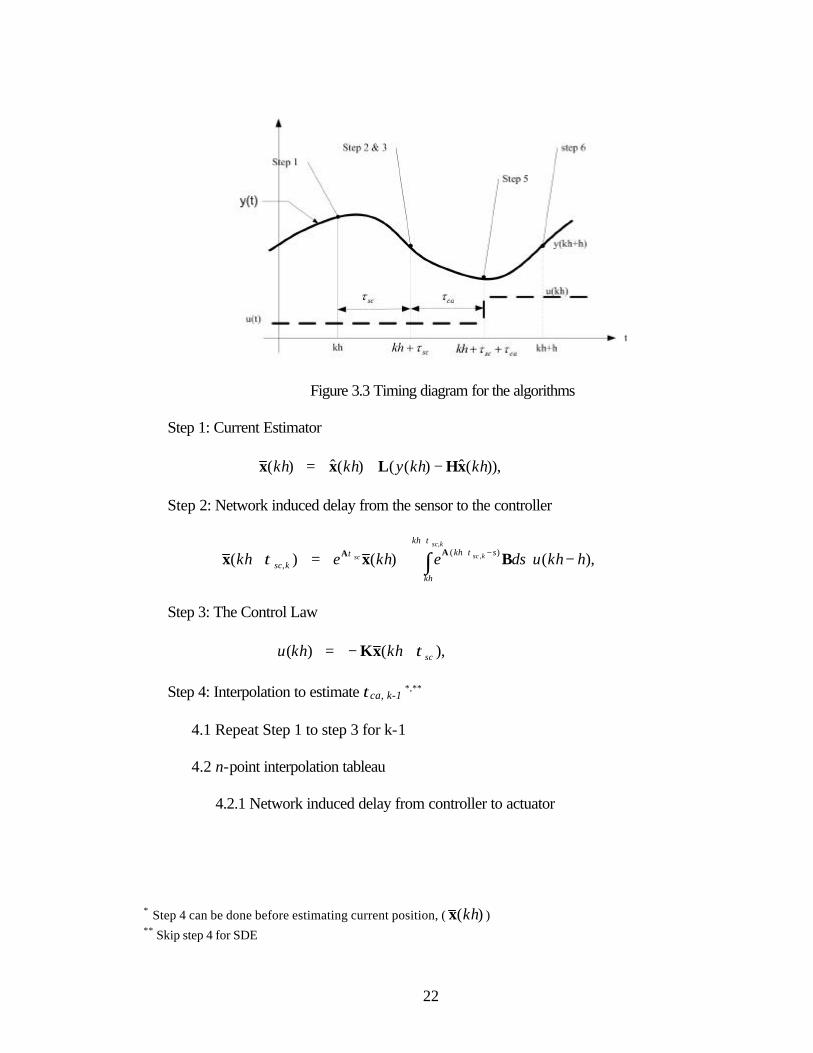
Figure 3.3 Timing diagram for the algorithms
Step 1: Current Estimator
)),(ˆ)(()(ˆ)( khkhykhkh xHLxx −+=
Step 2: Network induced delay from the sensor to the controller
∫+
−+ −⋅+=+ksc
kscsc
kh
kh
skhksc hkhudsekhekh
,
, ),()()( )(,
ττττ Bxx
AA
Step 3: The Control Law
),()( sckhkhu τ+−= xK
Step 4: Interpolation to estimate τca, k-1 *,**
4.1 Repeat Step 1 to step 3 for k-1
4.2 n-point interpolation tableau
4.2.1 Network induced delay from controller to actuator
∗ Step 4 can be done before estimating current position, ( )(khx ) ** Skip step 4 for SDE
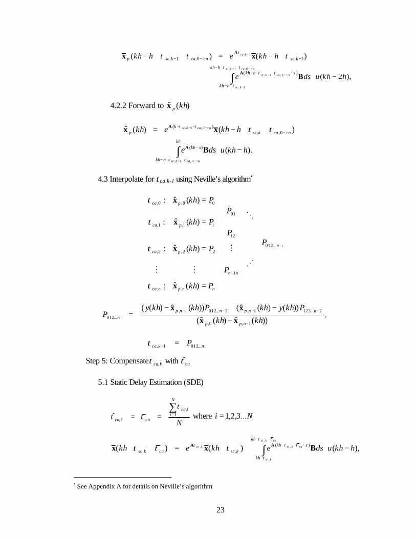
23
∫
>−−
−
>−−
−
++−
+−
−++−
−>−−
−⋅
++−=++−ncaksc
ksc
ncaksc
kca
hkh
hkh
shkh
kscncakscp
hkhudse
hkhehkh0,1,
1,
0,1,
1,
),2(
)()(
)(
1,0,1,
ττ
τ
ττ
τ τττ
B
xx
A
A
4.2.2 Forward to )(ˆ khpx
∫
>−−
>−−
++−
−
>−−−
−⋅
+++−=kh
hkh
skh
ncaksch
p
ncaksc
ncaksc
hkhudse
hkhekh
0,1,
0,1,
).(
)()(ˆ
)(
0,,)(
ττ
ττ ττ
B
xx
A
A
4.3 Interpolate for τca,k-1 using Neville’s algorithm•
nnpnca
nn
npca
pca
pca
Pkh
P
PPkh
P
PPkh
Pkh
=
=
=
=
−
)(ˆ:
)(ˆ:
)(ˆ:
)(ˆ:
,,
1
...01222,2,
12
01
11,1,
00,0,
x
x
x
x
τ
τ
τ
τ
NMM
M
O
,
))(ˆ)(ˆ(
))()(ˆ())(ˆ)((
1,0,
2...1231,2...0121,...012 khkh
PkhykhPkhkhyP
npp
nnpnnpn
−
−−−−
−
−+−=
xx
xx,
....0121, nkca P=−τ
Step 5: Compensate kca,τ with caτ̂
5.1 Static Delay Estimation (SDE)
N
N
iica
cakca
∑=== 1
,
,ˆτ
ττ where Ni ...3,2,1=
∫++
+
−++ −⋅++=++caksc
ksc
caksckca
kh
kh
skhksccaksc hkhudsekhekh
ττ
τ
τττ τττ,
,
,, ),()()( )(,, Bxx AA
• See Appendix A for details on Neville’s algorithm
24
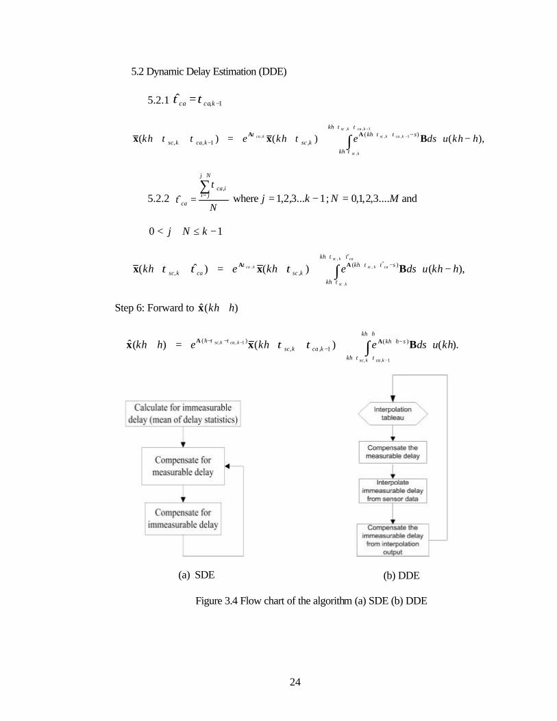
5.2 Dynamic Delay Estimation (DDE)
5.2.1 1,ˆ −= kcaca ττ
∫−
−
++
+
−++− −⋅++=++
1,,
,
1,,, ),()()( )(,1,,
kcaksc
ksc
kcaksckca
kh
kh
skhksckcaksc hkhudsekhekh
ττ
τ
τττ τττ Bxx AA
5.2.2 N
Nj
jiica
ca
∑+
==,
ˆτ
τ where 1...3,2,1 −= kj ; MN ....3,2,1,0= and
10 −≤+< kNj
∫++
+
−++ −⋅++=++caksc
ksc
caksckca
kh
kh
skhksccaksc hkhudsekhekh
ττ
τ
τττ τττˆ
)ˆ(,,
,
,
,, ),()()ˆ( Bxx AA
Step 6: Forward to )(ˆ hkh+x
∫+
++
−+−
−−
−
− ⋅+++=+hkh
kh
shkhkcaksc
h
kcaksc
kcaksc khudsekhehkh1,,
1,, ).()()(ˆ )(1,,
)(
ττ
ττ ττ Bxx AA
(a) SDE
(b) DDE
Figure 3.4 Flow chart of the algorithm (a) SDE (b) DDE
25
Explanation of these equations is as follow. At Step 1, the estimator corrects and
updates its states, and passing the result (via network) to controller. The time it takes for
the information transmission from Step 1 to Step 2 is induced by network traffic (τsc).
After compensated for τsc in Step 2, controller calculates updated control signal (Step 3).
At Step 4, the interpolation tableau is calculated (reminder: sensor and actuator do not
possess computational ability).
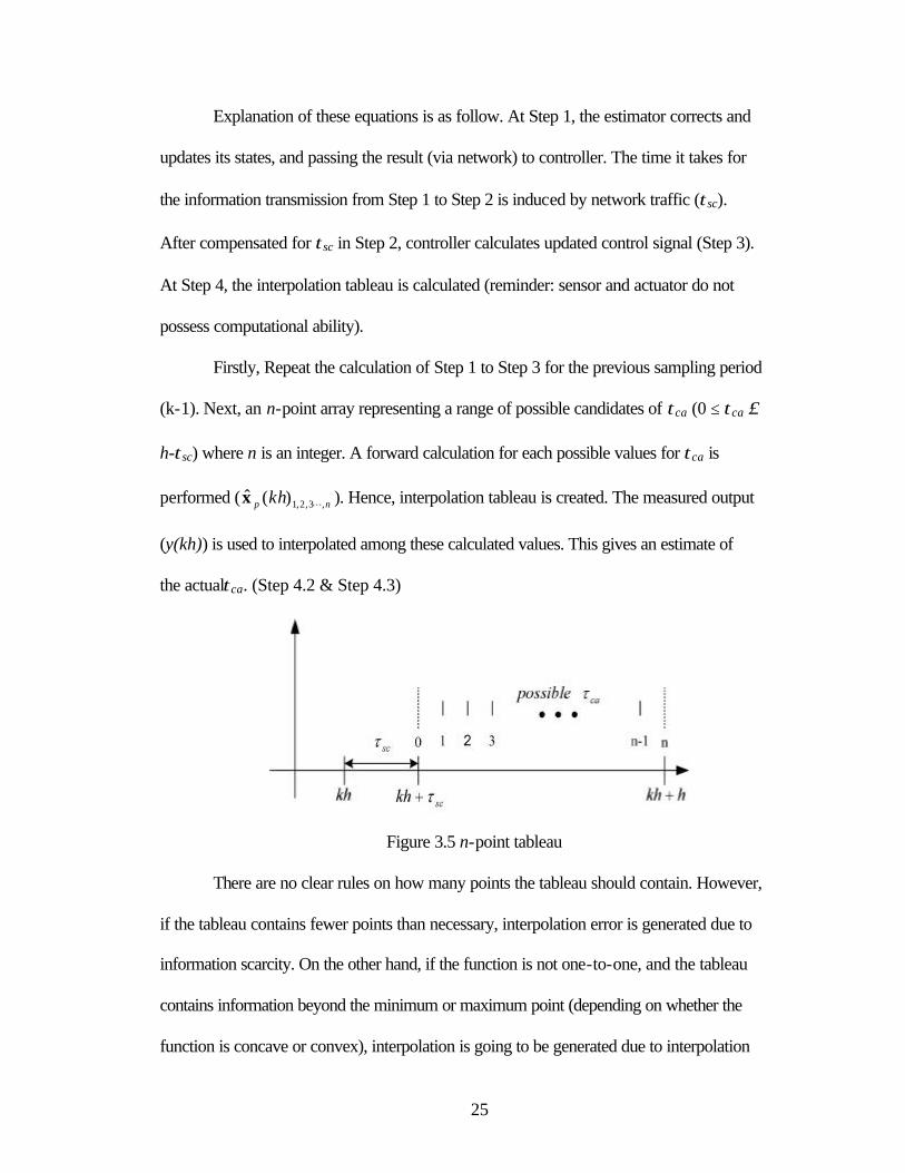
Firstly, Repeat the calculation of Step 1 to Step 3 for the previous sampling period
(k-1). Next, an n-point array representing a range of possible candidates of τca (0 ≤ τca ≤
h-τsc) where n is an integer. A forward calculation for each possible values for τca is
performed ( np kh ,3,2,1)(ˆLx ). Hence, interpolation tableau is created. The measured output
(y(kh)) is used to interpolated among these calculated values. This gives an estimate of
the actualτca. (Step 4.2 & Step 4.3)
Figure 3.5 n-point tableau
There are no clear rules on how many points the tableau should contain. However,
if the tableau contains fewer points than necessary, interpolation error is generated due to
information scarcity. On the other hand, if the function is not one-to-one, and the tableau
contains information beyond the minimum or maximum point (depending on whether the
function is concave or convex), interpolation is going to be generated due to interpolation
26
nature. (Consult results and discussions section in Real-time experiments for graphic
details.)
Compensate the system with the result from Step 4.3 (for DDE) or Step 5.1 (for
SDE). Lastly, predict result of Step 5 using the caτ̂ (Step 6).
Offline Experiments
Reviewed in Chapter 1 and Chapter 2, each network protocols give different delay
characteristics depending on their MAC-sublayer algorithms. In [6], the study conducted
various CAN and Ethernet network environments and measured the network-induced
delays from each setup. Inspired by that study, we created arrays of delays emulated from
those various scenarios and used our algorithms (either SDE or DDE) to compensate for
the τca.
We implemented our algorithms on a double integrator system. Its step-responses
were designed to exhibit characteristics of ς = 0.5 and ωn = 1.5784 rad/sec. The state
space of this double integrator is
).(1
0)(
00
10)( tutt
+
= xx&
Let the system be sampled with zero-order hold at the rate of T second/sampling
).(2
)(10
1)(
2
kTuT
TkT
TTkT
+
=+ xx
Constructing the estimator for the double integrator with compensation for τsc and
τca from the algorithms is as follows:
1. Estimator Correction
27
[ ][ ])(ˆ10)()(ˆ)(2
1 kTkTyLL
kTkT xxx ⋅−⋅
+= ,
2. Network induced delay from the sensor to the controller
)(2)(10
1)(
,
2,
,, TkTukTkT
ksc
kscksc
ksc −⋅
+⋅
=+
τ
τττ xx ,
3. The control law
[ ] )()( ,21 ksckTKKkTu τ+⋅−= x ,
4. Network induced delay from the controller to the actuator†
)(2)(10
1)(
*
2*
,
**
, TkTukTkT
ca
ca
kscca
caksc −⋅
++⋅
=++
τ
ττ
τττ xx ,
5. Forward to next sample‡
)(2
)(
2)(10
1)(ˆ
*,
*,
2*,
2
*,
*, kTu
T
TTT
kThTkT
caksc
caksccaksc
caksccaksc ⋅
−−
−−+
++++⋅
−−=+ττ
ττττ
ττττxx .
Using Matlab, the controller gain, K, and estimator gain, L, were calculated. Our
controller gain, K, was [ ]5208.17728.1 . In [3], it is suggested that responses from
estimators are conventionally two to four times faster than the response from the
controller. Here, we chose it to be two times faster. Correspondingly, the estimator gain,
L, was
−5857.1
4997.0. Also, the interpolations for τca in this section were aided by a
† *
caτ is caτ for SDE, and 1, −kcaτ for DDE
‡ *
caτ is caτ for SDE, and 1, −kcaτ for DDE
28
function in MATLAB called “interp1.m”. The results from DDE in this section were
interpolated from twenty-point tableau.
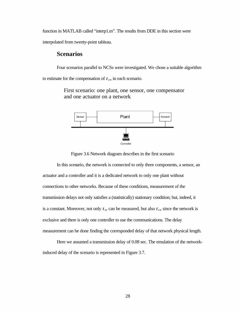
Scenarios
Four scenarios parallel to NCSs were investigated. We chose a suitable algorithm
to estimate for the compensation of τca in each scenario.
First scenario: one plant, one sensor, one compensator and one actuator on a network
Figure 3.6 Network diagram describes in the first scenario
In this scenario, the network is connected to only three components, a sensor, an
actuator and a controller and it is a dedicated network to only one plant without
connections to other networks. Because of these conditions, measurement of the
transmission delays not only satisfies a (statistically) stationary condition; but, indeed, it
is a constant. Moreover, not only τsc can be measured, but also τca since the network is
exclusive and there is only one controller to use the communications. The delay
measurement can be done finding the corresponded delay of that network physical length.
Here we assumed a transmission delay of 0.08 sec. The emulation of the network-
induced delay of the scenario is represented in Figure 3.7.
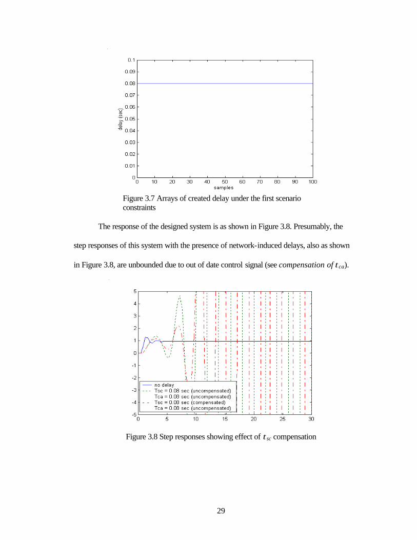
29
Figure 3.7 Arrays of created delay under the first scenario constraints
The response of the designed system is as shown in Figure 3.8. Presumably, the
step responses of this system with the presence of network-induced delays, also as shown
in Figure 3.8, are unbounded due to out of date control signal (see compensation of τca).
Figure 3.8 Step responses showing effect of τsc compensation
30
Even though the responses in Figure 3.8 for both of the τsc–uncompensated
system and the τsc–compensated system diverged, the τsc–compensated system diverged
at slower rate than the uncompensated system.
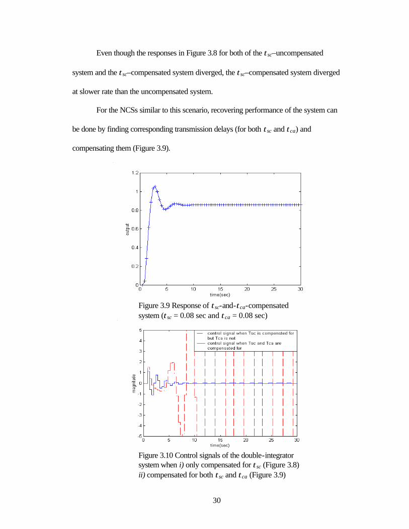
For the NCSs similar to this scenario, recovering performance of the system can
be done by finding corresponding transmission delays (for both τsc and τca) and
compensating them (Figure 3.9).
Figure 3.9 Response of τsc-and-τca-compensated system (τsc = 0.08 sec and τca = 0.08 sec)
Figure 3.10 Control signals of the double-integrator system when i) only compensated for τsc (Figure 3.8)
ii) compensated for both τsc and τca (Figure 3.9)
31
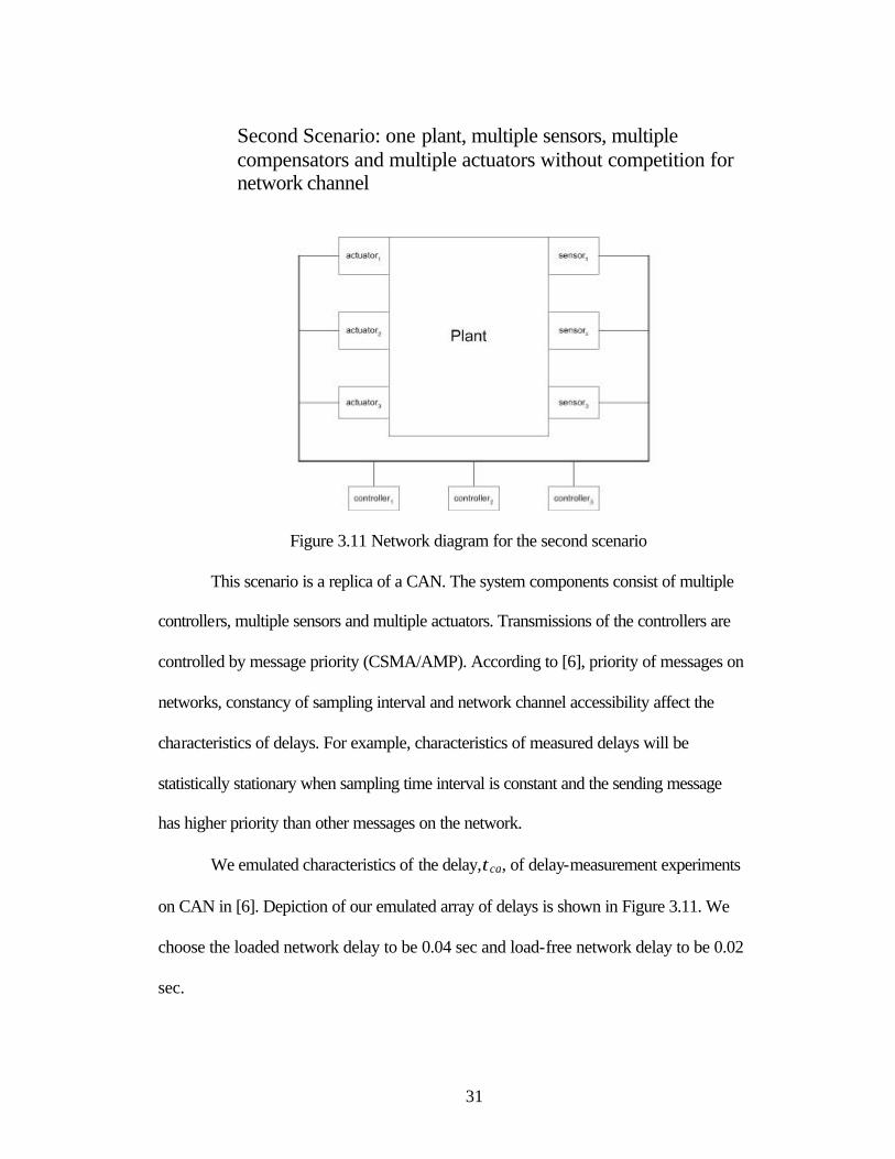
Second Scenario: one plant, multiple sensors, multiple compensators and multiple actuators without competition for network channel
Figure 3.11 Network diagram for the second scenario
This scenario is a replica of a CAN. The system components consist of multiple
controllers, multiple sensors and multiple actuators. Transmissions of the controllers are
controlled by message priority (CSMA/AMP). According to [6], priority of messages on
networks, constancy of sampling interval and network channel accessibility affect the
characteristics of delays. For example, characteristics of measured delays will be
statistically stationary when sampling time interval is constant and the sending message
has higher priority than other messages on the network.
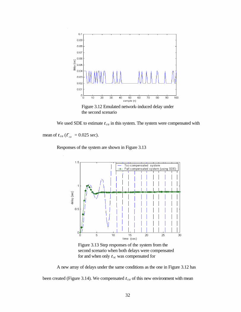
We emulated characteristics of the delay,τca, of delay-measurement experiments
on CAN in [6]. Depiction of our emulated array of delays is shown in Figure 3.11. We
choose the loaded network delay to be 0.04 sec and load-free network delay to be 0.02
sec.
32
Figure 3.12 Emulated network-induced delay under the second scenario
We used SDE to estimate τca in this system. The system were compensated with
mean of τca ( caτ = 0.025 sec).
Responses of the system are shown in Figure 3.13
Figure 3.13 Step responses of the system from the second scenario when both delays were compensated for and when only τsc was compensated for
A new array of delays under the same conditions as the one in Figure 3.12 has
been created (Figure 3.14). We compensated τca of this new environment with mean
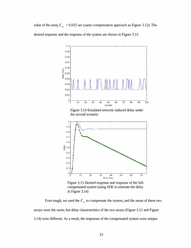
33
value of the array, caτ = 0.025 sec (same compensation approach as Figure 3.12). The
desired response and the response of the system are shown in Figure 3.15.
Figure 3.14 Emulated network-induced delay under the second scenario
Figure 3.15 Desired response and response of the full-compensated system (using SDE to estimate the delay in Figure 3.14)
Even tough, we used the caτ to compensate the system, and the mean of these two
arrays were the same, but delay characteristics of the two arrays (Figure 3.12 and Figure
3.14) were different. As a result, the responses of the compensated system were unique.
34
Surprisingly, the response of the system with the new array of delay could not be
recovered. This is because we compensated τca with “static” values. As shown in Figure
3.14, τca was a time-varying function, therefore; using single number to represent the
array of variety might not be an effective approach for that the precision of control
signals depending on this calculation.
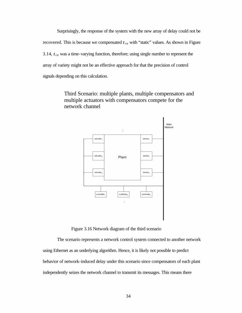
Third Scenario: multiple plants, multiple compensators and multiple actuators with compensators compete for the network channel
Figure 3.16 Network diagram of the third scenario
The scenario represents a network control system connected to another network
using Ethernet as an underlying algorithm. Hence, it is likely not possible to predict
behavior of network-induced delay under this scenario since compensators of each plant
independently seizes the network channel to transmit its messages. This means there
35
might be times that multiple compensators try to transmit data simultaneously; it might
also mean there is no channel usage at all. The uncertainty surely affects the estimate for
τca.
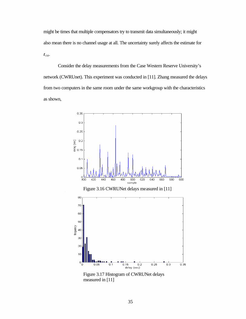
Consider the delay measurements from the Case Western Reserve University’s
network (CWRUnet). This experiment was conducted in [11]. Zhang measured the delays
from two computers in the same room under the same workgroup with the characteristics
as shown,
Figure 3.16 CWRUNet delays measured in [11]
Figure 3.17 Histogram of CWRUNet delays measured in [11]
36
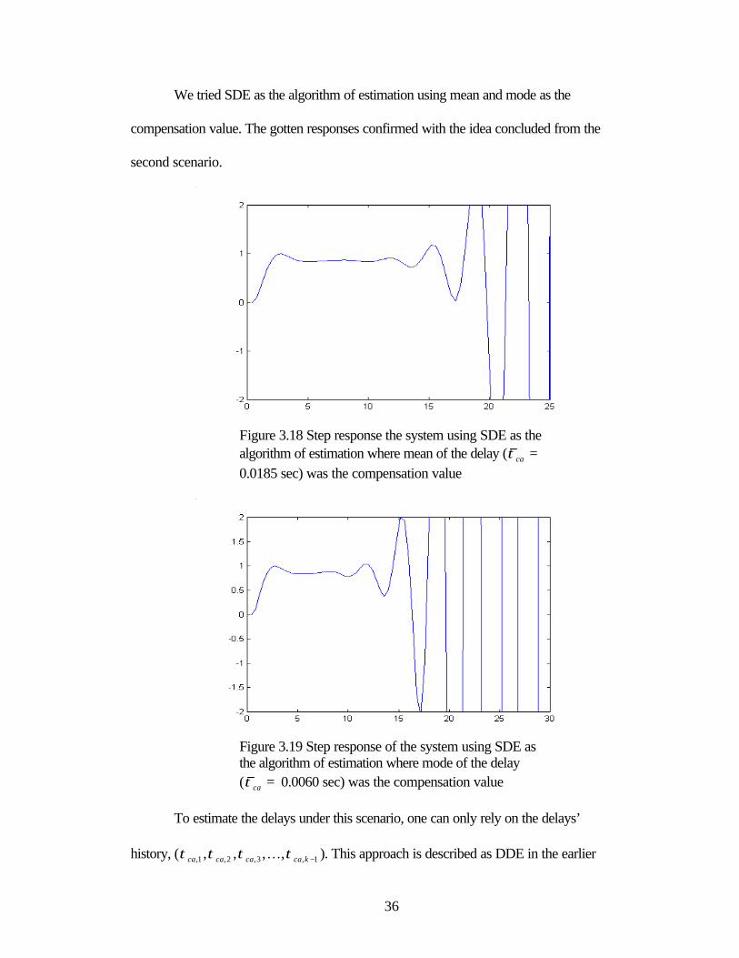
We tried SDE as the algorithm of estimation using mean and mode as the
compensation value. The gotten responses confirmed with the idea concluded from the
second scenario.
Figure 3.18 Step response the system using SDE as the algorithm of estimation where mean of the delay ( =caτ 0.0185 sec) was the compensation value
Figure 3.19 Step response of the system using SDE as the algorithm of estimation where mode of the delay ( =caτ 0.0060 sec) was the compensation value
To estimate the delays under this scenario, one can only rely on the delays’
history, ( 1,3,2,1, ,,,, −kcacacaca ττττ K ). This approach is described as DDE in the earlier
37
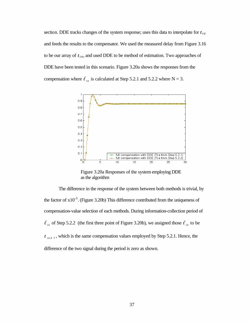
section. DDE tracks changes of the system response; uses this data to interpolate for τca
and feeds the results to the compensator. We used the measured delay from Figure 3.16
to be our array of τca, and used DDE to be method of estimation. Two approaches of
DDE have been tested in this scenario. Figure 3.20a shows the responses from the
compensation where caτ̂ is calculated at Step 5.2.1 and 5.2.2 where N = 3.
Figure 3.20a Responses of the system employing DDE as the algorithm
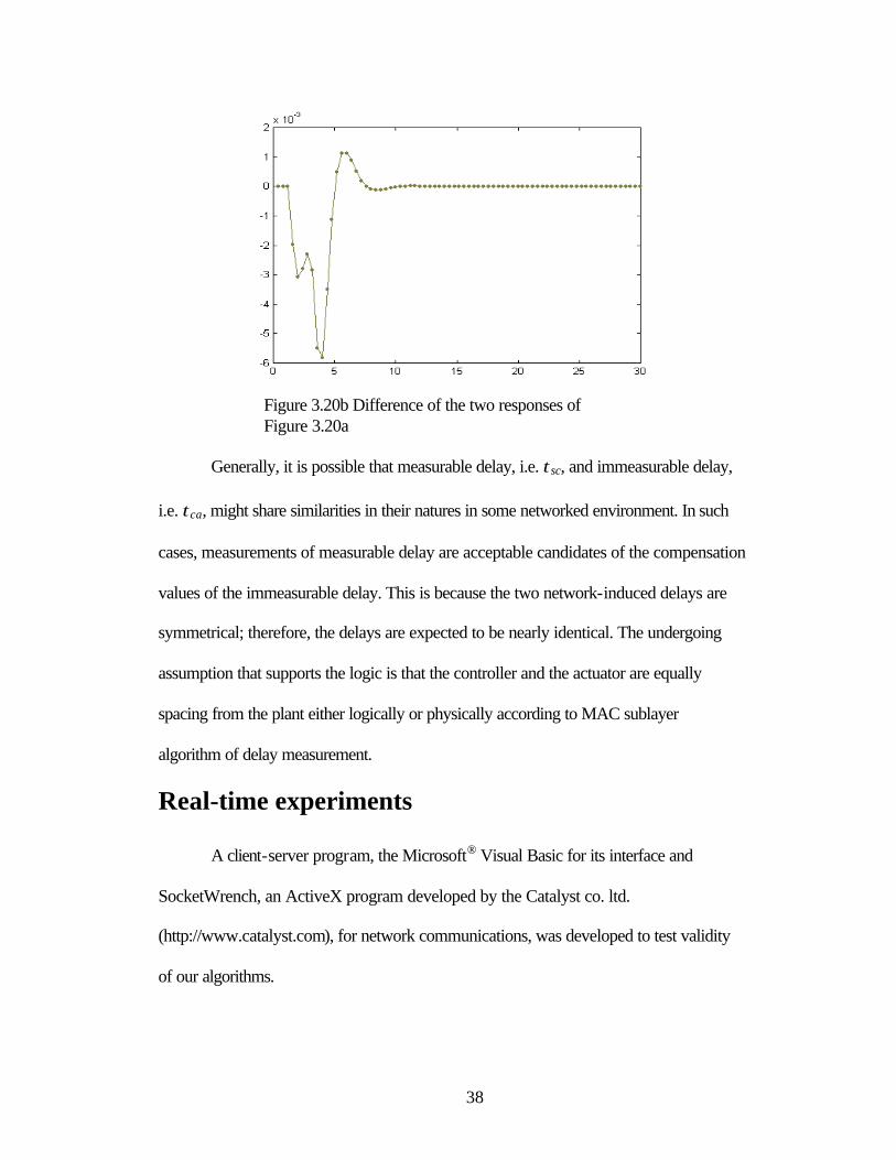
The difference in the response of the system between both methods is trivial, by
the factor of x10-3. (Figure 3.20b) This difference contributed from the uniqueness of
compensation-value selection of each methods. During information-collection period of
caτ̂ of Step 5.2.2 (the first three point of Figure 3.20b), we assigned those caτ̂ to be
1, −kcaτ , which is the same compensation values employed by Step 5.2.1. Hence, the
difference of the two signal during the period is zero as shown.
38
Figure 3.20b Difference of the two responses of Figure 3.20a
Generally, it is possible that measurable delay, i.e. τsc, and immeasurable delay,
i.e. τca, might share similarities in their natures in some networked environment. In such
cases, measurements of measurable delay are acceptable candidates of the compensation
values of the immeasurable delay. This is because the two network-induced delays are
symmetrical; therefore, the delays are expected to be nearly identical. The undergoing
assumption that supports the logic is that the controller and the actuator are equally
spacing from the plant either logically or physically according to MAC sublayer
algorithm of delay measurement.
Real-time experiments
A client-server program, the Microsoft® Visual Basic for its interface and
SocketWrench, an ActiveX program developed by the Catalyst co. ltd.
(http://www.catalyst.com), for network communications, was developed to test validity
of our algorithms.
39
The difference between this program and the program in [11] are this is a
standalone program and the algorithm behinds the two are different. In this program, the
computation is done by calling dynamic library link files (DLLs) while in [11] the
program relies on MATLAB for its computational ability. Moreover, the program in [11]
is conducted under the assumption of the delays (τsc and τca) were bundled together and
then compensated as measurable delays whereas in this program the delays were
differentiated to be measurable (e.g. τsc) and immeasurable delay (e.g. τca).
Clock Synchronization
There are several ways to synchronize the clocks, e.g. hardware synchronization,
software synchronization or combination of the both. This program used the scheme
reviewed in [2] & [11]; compensators send special signals to plants asking for clock
readings; the plants send the readings back to the compensators. The compensators
update their clocks with correction of the offset and round trip time.
Every message in this experiment sent out by the plant and the compensator is
time stamped for precise calculation for τsc; therefore, the plant and the compensator
clocks have to be synchronized.
Set-up
The program was set up on two computers, one as a plant (computer 1) and the
other as a compensator (computer 2). On the compensator side, we developed two
dynamic library links (DLLs), ctrl.dll1 and dbinte.dll2, to compute the control law and to
simulate the plant. In order to compensate immeasurable delay, we developed another
DLL called interp.dll3 to take care of the interpolation. 1 , 2, 3 Source codes are shown in Appendix B
40
Figure 3.21 Network diagram of the experiment
Figure 3.22 Logical diagram of the experiment
Results and Discussions
Step Input
We used the same double integrator to be the plant of this experiment. We ran the
experiment over the CWRUNet and used DDE for delay compensation with the desired
response as shown in Figure 3.8. The results from real-time experiments agreed with the
MATLAB experiment (offline experiment). This confirmed the validity of our algorithm
validity. The step response from our real-time experiments is as show in Figure 3.23.
41
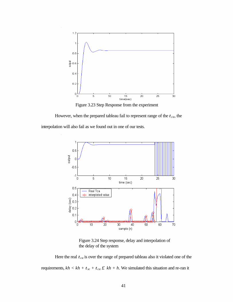
Figure 3.23 Step Response from the experiment
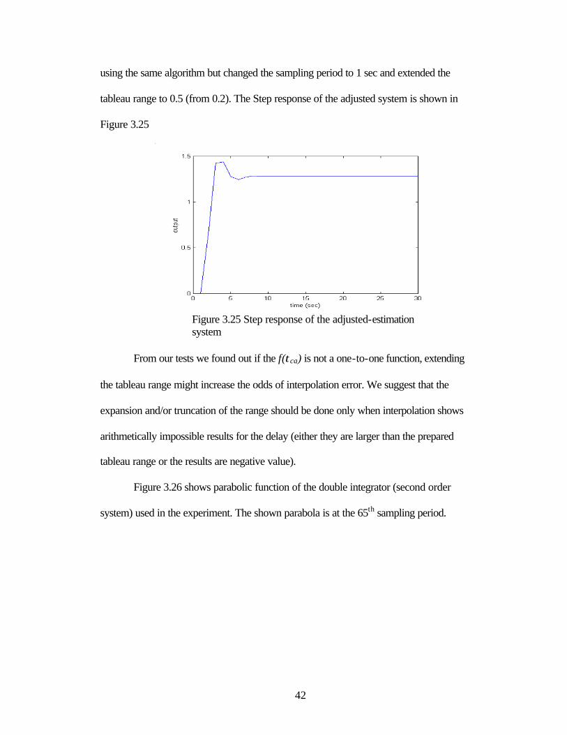
However, when the prepared tableau fail to represent range of the τca, the
interpolation will also fail as we found out in one of our tests.
Figure 3.24 Step response, delay and interpolation of the delay of the system
Here the real τca is over the range of prepared tableau also it violated one of the
requirements, kh < kh + τsc + τca ≤ kh + h. We simulated this situation and re-ran it
42
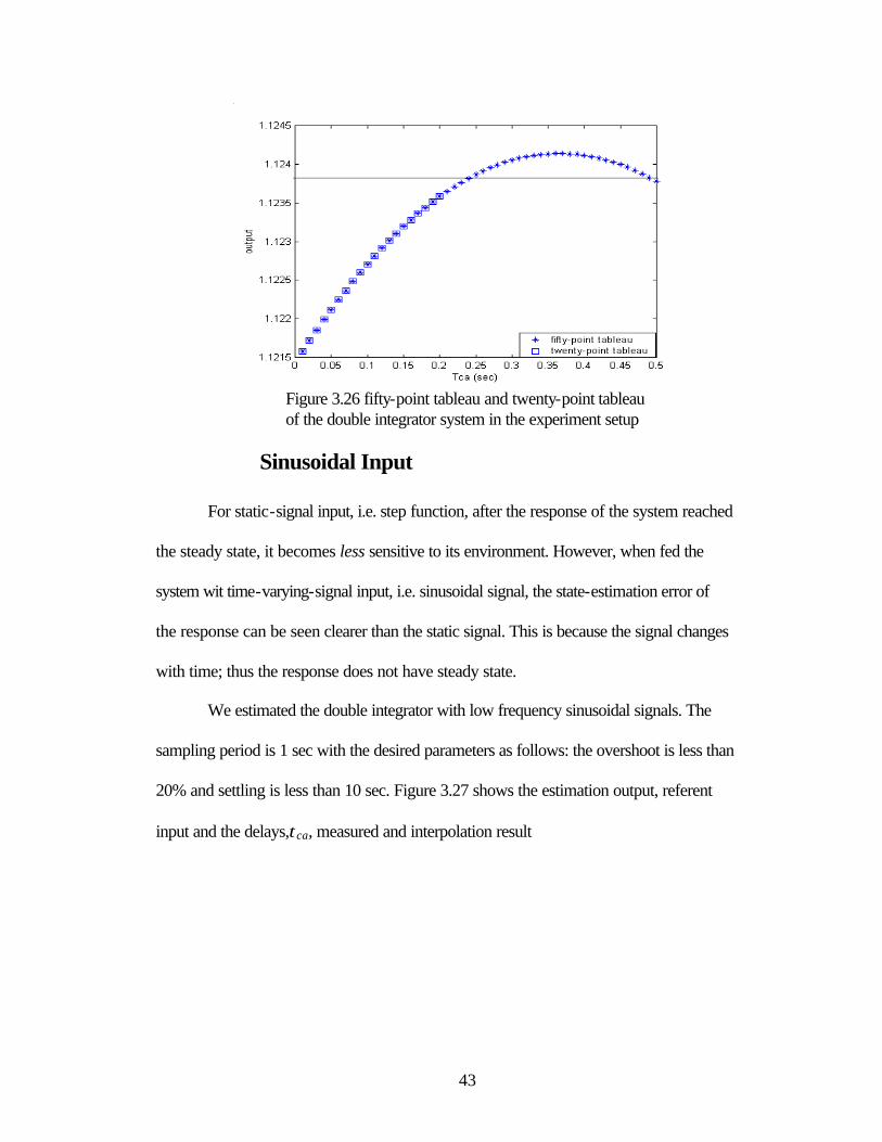
using the same algorithm but changed the sampling period to 1 sec and extended the
tableau range to 0.5 (from 0.2). The Step response of the adjusted system is shown in
Figure 3.25
Figure 3.25 Step response of the adjusted-estimation system
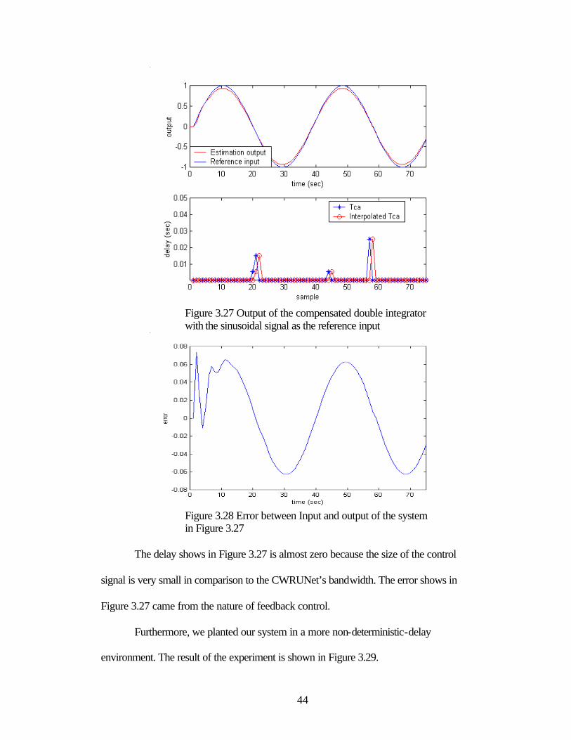
From our tests we found out if the f(τca) is not a one-to-one function, extending
the tableau range might increase the odds of interpolation error. We suggest that the
expansion and/or truncation of the range should be done only when interpolation shows
arithmetically impossible results for the delay (either they are larger than the prepared
tableau range or the results are negative value).
Figure 3.26 shows parabolic function of the double integrator (second order
system) used in the experiment. The shown parabola is at the 65th sampling period.
43
Figure 3.26 fifty-point tableau and twenty-point tableau of the double integrator system in the experiment setup
Sinusoidal Input
For static-signal input, i.e. step function, after the response of the system reached
the steady state, it becomes less sensitive to its environment. However, when fed the
system wit time-varying-signal input, i.e. sinusoidal signal, the state-estimation error of
the response can be seen clearer than the static signal. This is because the signal changes
with time; thus the response does not have steady state.
We estimated the double integrator with low frequency sinusoidal signals. The
sampling period is 1 sec with the desired parameters as follows: the overshoot is less than
20% and settling is less than 10 sec. Figure 3.27 shows the estimation output, referent
input and the delays,τca, measured and interpolation result
44
Figure 3.27 Output of the compensated double integrator with the sinusoidal signal as the reference input
Figure 3.28 Error between Input and output of the system in Figure 3.27
The delay shows in Figure 3.27 is almost zero because the size of the control
signal is very small in comparison to the CWRUNet’s bandwidth. The error shows in
Figure 3.27 came from the nature of feedback control.
Furthermore, we planted our system in a more non-deterministic-delay
environment. The result of the experiment is shown in Figure 3.29.
45
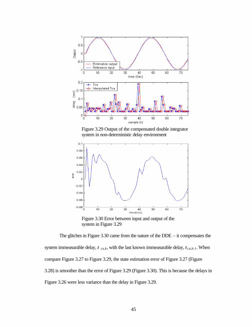
Figure 3.29 Output of the compensated double integrator system in non-deterministic delay environment
Figure 3.30 Error between input and output of the system in Figure 3.29
The glitches in Figure 3.30 came from the nature of the DDE – it compensates the
system immeasurable delay, τ ca,k, with the last known immeasurable delay, τca,k-1. When
compare Figure 3.27 to Figure 3.29, the state estimation error of Figure 3.27 (Figure
3.28) is smoother than the error of Figure 3.29 (Figure 3.30). This is because the delays in
Figure 3.26 were less variance than the delay in Figure 3.29.
46
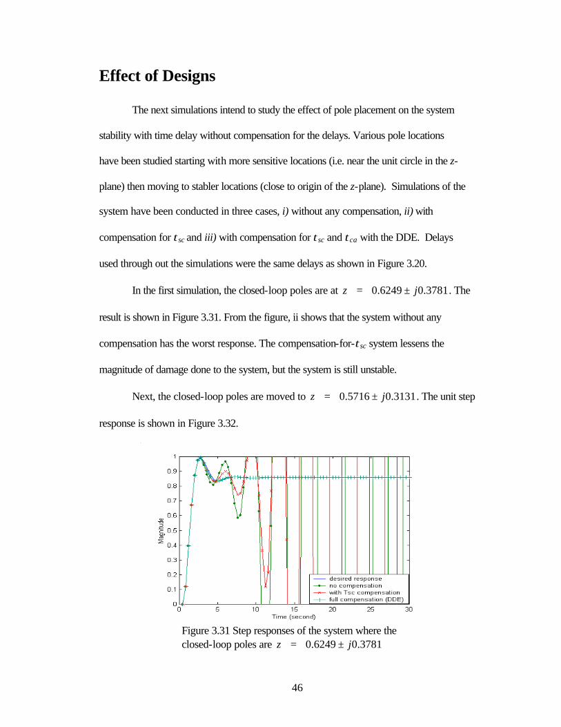
Effect of Designs
The next simulations intend to study the effect of pole placement on the system
stability with time delay without compensation for the delays. Various pole locations
have been studied starting with more sensitive locations (i.e. near the unit circle in the z-
plane) then moving to stabler locations (close to origin of the z-plane). Simulations of the
system have been conducted in three cases, i) without any compensation, ii) with
compensation for τsc and iii) with compensation for τsc and τca with the DDE. Delays
used through out the simulations were the same delays as shown in Figure 3.20.
In the first simulation, the closed-loop poles are at 3781.06249.0 jz ±= . The
result is shown in Figure 3.31. From the figure, ii shows that the system without any
compensation has the worst response. The compensation-for-τsc system lessens the
magnitude of damage done to the system, but the system is still unstable.
Next, the closed-loop poles are moved to 3131.05716.0 jz ±= . The unit step
response is shown in Figure 3.32.
Figure 3.31 Step responses of the system where the closed-loop poles are 3781.06249.0 jz ±=
47
Figure 3.32 Step responses of the system where the closed-loop poles located at 3131.05716.0 jz ±=
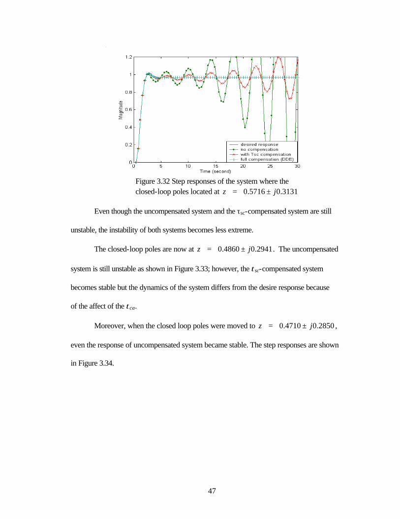
Even though the uncompensated system and the τsc-compensated system are still
unstable, the instability of both systems becomes less extreme.
The closed-loop poles are now at 2941.04860.0 jz ±= . The uncompensated
system is still unstable as shown in Figure 3.33; however, the τsc-compensated system
becomes stable but the dynamics of the system differs from the desire response because
of the affect of the τca.
Moreover, when the closed loop poles were moved to 2850.04710.0 jz ±= ,
even the response of uncompensated system became stable. The step responses are shown
in Figure 3.34.
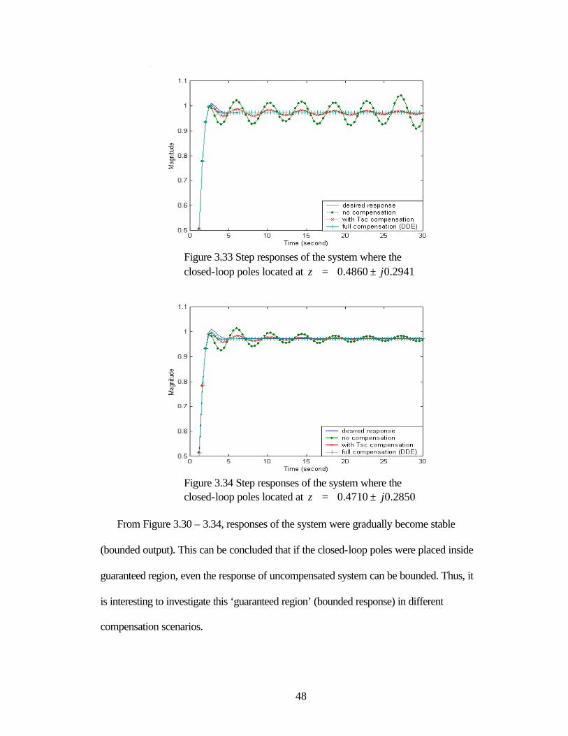
48
Figure 3.33 Step responses of the system where the closed-loop poles located at 2941.04860.0 jz ±=
Figure 3.34 Step responses of the system where the closed-loop poles located at 2850.04710.0 jz ±=
From Figure 3.30 – 3.34, responses of the system were gradually become stable
(bounded output). This can be concluded that if the closed-loop poles were placed inside
guaranteed region, even the response of uncompensated system can be bounded. Thus, it
is interesting to investigate this ‘guaranteed region’ (bounded response) in different
compensation scenarios.
49
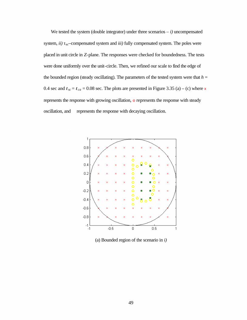
We tested the system (double integrator) under three scenarios – i) uncompensated
system, ii) τsc–compensated system and iii) fully compensated system. The poles were
placed in unit circle in Z-plane. The responses were checked for boundedness. The tests
were done uniformly over the unit-circle. Then, we refined our scale to find the edge of
the bounded region (steady oscillating). The parameters of the tested system were that h =
0.4 sec and τsc = τca = 0.08 sec. The plots are presented in Figure 3.35 (a) – (c) where x
represents the response with growing oscillation, o represents the response with steady
oscillation, and � represents the response with decaying oscillation.
(a) Bounded region of the scenario in i)
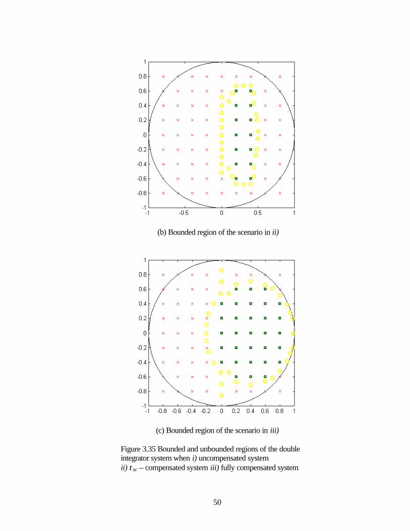
50
(b) Bounded region of the scenario in ii)
(c) Bounded region of the scenario in iii)
Figure 3.35 Bounded and unbounded regions of the double integrator system when i) uncompensated system ii) τsc – compensated system iii) fully compensated system
51
Chapter 4
Summary
For deterministic-delay networks, compensating the system by using mean values
of the delays are sufficient to stabilize systems (SDE). It is, however, more complicate in
non-deterministic-delay networks. DDE is proposed to use in the situation. The approach
is to estimate the delays from current sampled data to determine the τca. Resulting in
estimating the delay from previous sampling period; nevertheless, the estimated delay
should not be much different from the real delay since it is the same network and the
estimation is contiguous from one sample to another. However, sporadic bursts in
network traffic are inevitable occurrence. The effect can be seen in form of glitches in the
response at the time burstiness occurred.
Position of pole placement may relieve severity of instability of the system in the
manner that when closed-loop poles are placed to stabler area, the systems are able
tolerate more disturbance (in the simulations the system becomes more tolerable to the
error accounted for the lack of compensation for τsc and/or τca). This leads to a topic of
greedy control. The realization is that when employ a greedy control, an accurate
estimator is crucial. Yet, there exist noises that may deteriorate proficiency of estimators.
Hence, we do not recommend the method of pole shifting to be solely solution for the
delay problem. However, deftly placing the poles would alleviate the problem. Yet,
choosing location for the poles is a form of art and there is no right or wrong as long as
the constraints were met. The way to master the skill is by observation and practices.
Moreover, stability region of the model NCS when compensations for ôsc and ôca are
absent is smallest but it grows as delays have been compensated. This confirms our

52
assumption that if immeasurable delay is left uncompensated, system response will
degrade.
53
Appendices
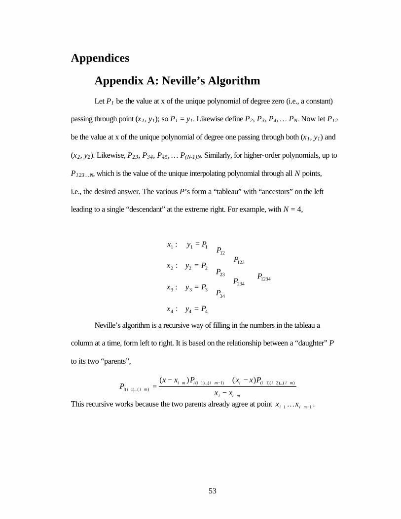
Appendix A: Neville’s Algorithm
Let P1 be the value at x of the unique polynomial of degree zero (i.e., a constant)
passing through point (x1, y1); so P1 = y1. Likewise define P2, P3, P4, … PN. Now let P12
be the value at x of the unique polynomial of degree one passing through both (x1, y1) and
(x2, y2). Likewise, P23, P34, P45, … P(N-1)N. Similarly, for higher-order polynomials, up to
P123…N, which is the value of the unique interpolating polynomial through all N points,
i.e., the desired answer. The various P’s form a “tableau” with “ancestors” on the left
leading to a single “descendant” at the extreme right. For example, with N = 4,
1234
444
234
34333
123
23222
12111
:
:
:
:
P
Pyx
PP
Pyx
PP
Pyx
PPyx
=
=
=
=
Neville’s algorithm is a recursive way of filling in the numbers in the tableau a
column at a time, form left to right. It is based on the relationship between a “daughter” P
to its two “parents”,
mii
miiiimiiimimiii xx
PxxPxxP
+
+++−+++++ −
−+−= ))...(2)(1()1)...(1(
))...(1(
)()(
This recursive works because the two parents already agree at point 11 −++ mii xx K .
54
Appendix B
Appendix B1: Source code for Plant
Option Explicit Private Type SysTime sysYear As Integer sysMonth As Integer sysDay As Integer sysDayofWeek As Integer sysHour As Integer sysMin As Integer sysSec As Integer sysMilliSec As Integer End Type Dim TestTime As SysTime, Delaycheck As SysTime Dim samples As Integer Dim Tsc(51) As Double, ctrl(51) As Double, Tca(51) As Double Dim x1 As Double, x2 As Double Dim Y2(51) As Double Private Declare Sub GetSystemTime Lib "kernel32" _ (lpSystemTime As SysTime) 'Plant caluculation function Private Declare Function dbintgX1Kh2Tsc Lib "dbinte" _ (ByVal x1 As Double, ByVal x2 As Double, ByVal sdelay As Double, ByVal ctls As Double) As Double Private Declare Function dbintgX2Kh2Tsc Lib "dbinte" _ (ByVal x2 As Double, ByVal sdelay As Double, ByVal ctls As Double) As Double Private Declare Function dbintgX1Tsc2Tca Lib "dbinte" _ (ByVal x1 As Double, ByVal x2 As Double, ByVal adelay As Double, ByVal ctls As Double) As Double Private Declare Function dbintgX2Tsc2Tca Lib "dbinte" _ (ByVal x2 As Double, ByVal adelay As Double, ByVal ctls As Double) As Double Private Declare Function dbintgX1Tca2H Lib "dbinte" _ (ByVal x1 As Double, ByVal x2 As Double, ByVal h As Double, ByVal sdelay As Double, ByVal adelay As Double, ByVal ctls As Double) As Double Private Declare Function dbintgX2Tca2H Lib "dbinte" _ (ByVal x2 As Double, ByVal h As Double, ByVal sdelay As Double, ByVal adelay As Double, ByVal ctls As Double) As Double Private Sub CnntButt_Click() ServerSock.AutoResolve = False If ServerSock.BindAddress = "" Then ServerSock.BindAddress = Trim(Plant_IP.Text) End If ServerSock.Blocking = False ServerSock.Binary = False ServerSock.SocketType = SOCK_STREAM ServerSock.BufferSize = 1024 ServerSock.LocalPort = CInt(Val(CtrlPort.Text)) Plant_IP.Enabled = False CtrlPort.Enabled = False If CnntButt.Caption = "Listen" Then CnntButt.Enabled = False ServerSock.Listen Else ServerSock.Action = SOCKET_CLOSE End If UpdateForm End Sub Private Sub DisconBtt_Click() If MsgBox("Are you sure you want to disconnect the controller?", vbQuestion + vbYesNo, App.Title) = vbNo Then Exit Sub
55
End If If ServerSock.Connected Then If MsgBox("Connection to be disconnect", vbYesNo) = vbNo Then Exit Sub Else ServerSock.Disconnect SamplingPeriod.Enabled = False End If Else MsgBox "Your connection hasn't been estrablished" End If ServerSock.Action = SOCKET_CLOSE Call Form_Load End Sub Private Sub Form_Load() Plant_IP.Text = "0.0.0.0" Controller_IP.Enabled = False Controller_IP.Text = "0.0.0.0" CtrlPort.Text = CLng(Val(IPPORT_ECHO)) Start.Enabled = True SamplingPeriod.Enabled = False samples = 1 Y1(0) = 0 Y1(1) = 0 Tsc(0) = 0 Tca(0) = 0 ctrl(0) = 0 End Sub Private Sub Gplot_Click() graph.Show End Sub Private Sub Plant_IP_Change() UpdateForm End Sub Private Sub Plant_IP_GotFocus() Plant_IP.SelStart = 0 Plant_IP.SelLength = Len(Plant_IP.Text) End Sub Private Sub Plant_IP_KeyPress(KeyAscii As Integer) If KeyAscii > 31 And KeyAscii <> 46 And (KeyAscii < 48 Or KeyAscii > 57) Then KeyAscii = 0: Beep End If End Sub Private Sub CtrlPort_Change() UpdateForm End Sub Private Sub CtrlPort_GotFocus() CtrlPort.SelStart = 0 CtrlPort.SelLength = Len(CtrlPort.Text) End Sub Private Sub CtrlPort_KeyPress(KeyAscii As Integer) If KeyAscii > 31 And KeyAscii <> 46 And (KeyAscii < 48 Or KeyAscii > 57) Then KeyAscii = 0: Beep End If End Sub Private Sub SamplingPeriod_Timer() x1 = dbintgX1Kh2Tsc(Y1(samples), Y2(samples), Tsc(samples), ctrl(samples)) x2 = dbintgX2Kh2Tsc(Y2(samples), Tsc(samples), ctrl(samples)) x1 = dbintgX1Tsc2Tca(x1, x2, Tca(samples), ctrl(samples)) x2 = dbintgX2Tsc2Tca(x2, Tca(samples), ctrl(samples))
56
Y1(samples + 1) = dbintgX1Tca2H(x1, x2, 0.4, Tsc(samples), Tca(samples), ctrl(samples + 1)) Y2(samples + 1) = dbintgX2Tca2H(x2, 0.4, Tsc(samples), Tsc(samples), ctrl(samples + 1)) samples = samples + 1 If samples > 50 Then SamplingPeriod.Enabled = False MsgBox "END", vbExclamation Call DisconBtt_Click Exit Sub End If Call SensorDelay End Sub Private Sub ServerSock_Accept(SocketId As Integer) If ServerSock.Listening Then ServerSock.Action = SOCKET_ACCEPT End If End Sub Private Sub ServerSock_Connect() MsgBox "Accepted connection from client at" & ServerSock.PeerAddress, vbOKOnly Controller_IP.Text = ServerSock.PeerAddress Controller_IP.Enabled = False UpdateForm End Sub Private Sub ServerSock_Disconnect() ServerSock.Disconnect MsgBox "Client disconnected" UpdateForm Call Form_Load End Sub Private Sub ServerSock_Read(DataLength As Integer, IsUrgent As Integer) Dim StrBuffer As String 'Change it to Float Dim uPosition As Integer ServerSock.Read StrBuffer, DataLength If InStr(1, Trim(StrBuffer), "y", 1) = 2 And InStr(1, Trim(StrBuffer), "k", 1) = 9 Then Call SyncClock Exit Sub Else uPosition = CInt(InStr(1, StrBuffer, "u", 1)) Tsc(samples) = CDbl(Mid(Trim(StrBuffer), 2, uPosition - 2)) ctrl(samples + 1) = CDbl(Mid(StrBuffer, uPosition + 1, DataLength - uPosition)) If SamplingPeriod.Enabled = False Then SamplingPeriod.Enabled = True End If FrmCtrller.Text = StrBuffer FrmCtrller.Refresh End If End Sub Private Sub UpdateForm() Dim strTitle As String, bEnable As Integer strTitle = App.Title bEnable = True If Len(Trim(Plant_IP.Text)) = 0 Then bEnable = False If Len(Trim(CtrlPort.Text)) = 0 Then bEnable = False If ServerSock.Listening Then CnntButt.Caption = "Pause" CnntButt.Enabled = False strTitle = strTitle & "Paused"
57
ElseIf ServerSock.Connected Then CnntButt.Caption = "Pause" CnntButt.Enabled = False Plant_IP.Enabled = False CtrlPort.Enabled = False Else CnntButt.Caption = "Listen" CnntButt.Enabled = bEnable Plant_IP.Enabled = True CtrlPort.Enabled = True End If FrmCtrller.Text = "" ToCtrller.Text = "" End Sub Private Sub SyncClock() Dim Wtime As Long Dim SentWtime As String GetSystemTime TestTime Wtime = (TestTime.sysHour * 3.6 + TestTime.sysMin * 0.06 _ + TestTime.sysSec * 0.001 + TestTime.sysMilliSec * 0.000001) * 1000000 SentWtime = ":" & CStr(Wtime) & ":" ServerSock.Write SentWtime, Len(SentWtime) End Sub Private Sub SensorDelay() Dim sendchk As Double Dim ToCtrller As String GetSystemTime Delaycheck sendchk = (Delaycheck.sysHour * CDbl(3600) + Delaycheck.sysMin * CDbl(60) + Delaycheck.sysSec _ + Delaycheck.sysMilliSec / 1000) 'clock in seconds ToCtrller = "@" & CStr(Y1(samples)) & "," & CStr(sendchk) ServerSock.Write ToCtrller, Len(ToCtrller) End Sub Private Sub Start_Click() Start.Enabled = False Call SensorDelay End Sub
Appendix B2: Source code for Controller Option Explicit Private Type SysTime sysYear As Integer sysMonth As Integer sysDayofWeek As Integer sysDay As Integer sysHour As Integer sysMin As Integer sysSec As Integer sysMilliSec As Integer End Type Dim TestSysTime As SysTime Dim xmitDelay As Single Dim Delay As SysTime Private Declare Sub GetSystemTime Lib "kernel32" _ (lpSystemTime As SysTime) Private Declare Sub SetSystemTime Lib "kernel32" _
58
(lpSystemTime As SysTime) 'Controller Private Declare Function contrl Lib "contrl.dll" _ (ByVal k1 As Double, ByVal k2 As Double, ByVal x1 As Double, ByVal x2 As Double, ByVal Input1 As Double, ByVal Input2 As Double) As Double 'Inerpolation Private Declare Sub interp Lib "interp.dll" _ (First() As Double, Second() As Double, ByVal pointX As Double, ByVal N As Integer, outcome As Double) 'Estimator Calculation Private Declare Function dbintgX1Kh2Tsc Lib "dbinte.dll" _ (ByVal x1 As Double, ByVal x2 As Double, ByVal sdelay As Double, ByVal ctls As Double) As Double Private Declare Function dbintgX2Kh2Tsc Lib "dbinte.dll" _ (ByVal x2 As Double, ByVal sdelay As Double, ByVal ctls As Double) As Double Private Declare Function dbintgX1Tsc2Tca Lib "dbinte.dll" _ (ByVal x1 As Double, ByVal x2 As Double, ByVal adelay As Double, ByVal ctls As Double) As Double Private Declare Function dbintgX2Tsc2Tca Lib "dbinte.dll" _ (ByVal x2 As Double, ByVal adelay As Double, ByVal ctls As Double) As Double Private Declare Function dbintgX1Tca2H Lib "dbinte.dll" _ (ByVal x1 As Double, ByVal x2 As Double, ByVal h As Double, ByVal sdelay As Double, ByVal adelay As Double, ByVal ctls As Double) As Double Private Declare Function dbintgX2Tca2H Lib "dbinte.dll" _ (ByVal x2 As Double, ByVal h As Double, ByVal sdelay As Double, ByVal adelay As Double, ByVal ctls As Double) As Double Dim Gtca(51) As Double, XE1(51) As Double, XE2(51) As Double Dim Tsc(51) As Double, Ctrl(51) As Double, Y(51) As Double Dim N As Integer Private Sub ClientSock_Connect() UpdateForm RcvSignal.Text = "" SndSignal.Text = "" SndSignal.SetFocus PortNo.Enabled = False PlantIP.Enabled = False End Sub Private Sub DisconBtt_Click() If ClientSock.Connected Then ClientSock.Disconnect MsgBox "Connection as been disconnected", vbOKOnly CnntBtt.Enabled = True Else MsgBox "No connection yet", vbOKOnly + vbExclamation If CnntBtt.Enabled = False Then CnntBtt.Enabled = True End If End If Call Form_Load End Sub Private Sub Form_Load() PortNo.Text = CInt(Val(IPPORT_ECHO)) PlantIP.Text = "0.0.0.0" RcvSignal.Text = "" SndSignal.Text = "" PortNo.Enabled = True PlantIP.Enabled = True N = 1 End Sub Private Sub CnntBtt_Click() CnntBtt.Enabled = False ClientSock.AddressFamily = AF_INET ClientSock.Protocol = IPPROTO_TCP
59
ClientSock.SocketType = SOCK_STREAM ClientSock.BufferSize = 1024 ClientSock.Binary = False ClientSock.RemotePort = Val(PortNo.Text) ClientSock.Blocking = False ClientSock.AutoResolve = False ClientSock.HostAddress = Trim(PlantIP.Text) ClientSock.Connect PortNo.Enabled = False PlantIP.Enabled = False End Sub Private Sub PlantIP_Change() UpdateForm End Sub Private Sub PlantIP_GotFocus() PlantIP.SelStart = 0 PlantIP.SelLength = Len(PlantIP.Text) End Sub Private Sub PlantIP_KeyPress(KeyAscii As Integer) If KeyAscii > 31 And KeyAscii <> 46 And (KeyAscii < 48 Or KeyAscii > 57) Then KeyAscii = 0: Beep End If End Sub Private Sub PortNo_Change() UpdateForm End Sub Private Sub PortNo_GotFocus() PortNo.SelStart = 0 PortNo.SelLength = Len(PortNo.Text) End Sub Private Sub PortNo_KeyPress(KeyAscii As Integer) If KeyAscii > 31 And KeyAscii <> 46 And (KeyAscii < 48 Or KeyAscii > 57) Then KeyAscii = 0: Beep End If End Sub Private Sub ClientSock_Read(DataLength As Integer, IsUrgent As Integer) Dim RStrBuffer As String Dim DelayBuffer As Double Dim dPosition As Integer Dim ctrlTime As Double ClientSock.Read RStrBuffer, DataLength If Left(RStrBuffer, 1) = ":" And Right(RStrBuffer, 1) = ":" Then Call SyncClock(RStrBuffer) Exit Sub Else dPosition = InStr(RStrBuffer, ",") Y(N) = CDbl(Mid(RStrBuffer, 2, dPosition - 2)) DelayBuffer = CDbl(Mid(RStrBuffer, dPosition + 1, Len(RStrBuffer) - dPosition)) GetSystemTime Delay ctrlTime = (Delay.sysHour * CDbl(3600) + Delay.sysMin * CDbl(60) + Delay.sysSec _ + Delay.sysMilliSec / CDbl(1000)) Tsc(N) = ctrlTime - DelayBuffer RcvSignal.SelLength = 0 RcvSignal.SelText = RStrBuffer RcvSignal.Refresh
60
Call ComputCtrller Exit Sub End If End Sub Private Sub UpdateForm() If ClientSock.Connected Then If Len(ClientSock.HostName) > 0 Then ThesisCtrl.Caption = ClientSock.HostName & " - " & App.Title Else ThesisCtrl.Caption = ClientSock.HostAddress & " - " & App.Title End If RcvSignal.Enabled = True End If End Sub Private Sub SyncButt_Click() Dim clkBuffer As String SyncButt.Enabled = True clkBuffer = "Syn Clock" ClientSock.Write clkBuffer, Len(clkBuffer) xmitDelay = Timer End Sub Private Sub SyncClock(WTime As String) Dim Rtime As String Dim TimeBuffer As Long Dim setHour As Integer Dim setMin As Integer Dim setSec As Integer Dim setMilliSec As Integer Rtime = (Mid(WTime, 2, Len(WTime) - 2)) xmitDelay = ((Timer - xmitDelay) * 1000) / 2 TimeBuffer = CLng(CLng(Rtime) + Int(xmitDelay)) setHour = TimeBuffer / 3600000 - (TimeBuffer Mod 3600000) / 3600000 setMin = (TimeBuffer - setHour * 3600000) / 60000 - _ ((TimeBuffer - setHour * 3600000) Mod 60000) / 60000 setSec = (TimeBuffer - setHour * 3600000 - setMin * 60000) / 1000 - _ ((TimeBuffer - setHour * 3600000 - setMin * 60000) Mod 1000) / 1000 setMilliSec = (TimeBuffer - setHour * 3600000 - setMin * 60000) Mod 1000 SetSystemTime TestSysTime TestSysTime.sysHour = setHour TestSysTime.sysMin = setMin TestSysTime.sysSec = setSec TestSysTime.sysMilliSec = setMilliSec MsgBox "Sync Done" End Sub Private Sub ComputCtrller() 'output is Yread right now we doing open loop est 'Varaibles have not been declare yet. Dim x1 As Double, x2 As Double Dim X1loop As Double, X2loop As Double Dim Guesstca As Double, Loopout() As Double, Tca() As Double Dim ToPlant As String, tcacount As Integer Tsc(0) = 0 XE1(0) = 0
61
XE2(0) = 0 Ctrl(0) = 0 Ctrl(1) = 0 x1 = dbintgX1Kh2Tsc(XE1(N), XE2(N), Tsc(N), Ctrl(N)) x2 = dbintgX2Kh2Tsc(XE2(N), Tsc(N), Ctrl(N)) 'compute Ctrl Signal Ctrl(N + 1) = contrl(2.1915, 2.1315, x1, x2, 0, 1) ToPlant = CStr("D" & Tsc(N) & "u" & Ctrl(N + 1)) ClientSock.Write ToPlant, Len(ToPlant) ReDim Tca(21) ReDim Loopout(20) Tca(1) = 0 If N > 1 Then For tcacount = 1 To 20 X1loop = dbintgX1Kh2Tsc(XE1(N - 1), XE2(N - 1), Tsc(N - 1), Ctrl(N - 1)) X2loop = dbintgX2Kh2Tsc(XE2(N - 1), Tsc(N - 1), Ctrl(N - 1)) X1loop = dbintgX1Tsc2Tca(X1loop, X2loop, Tca(tcacount), Ctrl(N - 1)) X2loop = dbintgX2Tsc2Tca(X2loop, Tca(tcacount), Ctrl(N - 1)) X1loop = dbintgX1Tca2H(X1loop, X2loop, 0.4, Tsc(N - 1), Tca(tcacount), Ctrl(N)) X2loop = dbintgX2Tca2H(X2loop, 0.4, Tsc(N - 1), Tca(tcacount), Ctrl(N)) Loopout(tcacount) = X1loop Tca(tcacount + 1) = Tca(tcacount) + (1 / 19#) Next tcacount ReDim Tca(20) Tca(1) = 0 For tcacount = 1 To 19 Tca(tcacount + 1) = Tca(tcacount) + (1 / 19#) Next tcacount interp(Loopout(), Tca(), Y(N), 20, Guesstca) = Gtca(N) Else Gtca(N) = 0 End If x1 = dbintgX1Tsc2Tca(x1, x2, Gtca(N), Ctrl(N)) x2 = dbintgX2Tsc2Tca(x2, Gtca(N), Ctrl(N)) x1 = dbintgX1Tca2H(x1, x2, 0.4, Tsc(N), Gtca(N), Ctrl(N + 1)) x2 = dbintgX2Tca2H(x2, 0.4, Tsc(N), Gtca(N), Ctrl(N + 1)) XE1(N + 1) = x1 + CDbl(0.0188) * (x1 - Y(N)) XE2(N + 1) = x2 + CDbl(0.8983) * (x2 - Y(N)) N = N + 1 End Sub
Appendix B3: Source code for DLLs contrl.dll controller.h # include <windows.h> # include <math.h> # include <stdlib.h> double __declspec(dllexport) __stdcall contrl(double k1, double k2, double x1, double x2, double inp1, double inp2); controller.c #include "controller.h"
62
double __declspec(dllexport) __stdcall contrl(double k1, double k2, double x1, double x2, double inp1, double inp2) { double ctls; ctls = k1*(-x1+inp1)+k2*(-x2+inp2); return(ctls); } controller.def LIBRARY contrl EXPORTS contrl dbinte.dll dbinte.h # include <windows.h> # include <math.h> #include <stdlib.h> double __declspec (dllexport) __stdcall dbintgX1Kh2Tsc(double X1, double X2, double Tsc, double ctrl); double __declspec (dllexport) __stdcall dbintgX2Kh2Tsc(double X2,double Tsc, double ctls); double __declspec (dllexport) __stdcall dbintgX1Tsc2Tca(double X1, double X2,double Tca, double ctls); double __declspec (dllexport) __stdcall dbintgX2Tsc2Tca(double X2,double Tca, double ctls); double __declspec (dllexport) __stdcall dbintgX1Tca2H(double X1, double X2,double h,double Tsc, double Tca, double ctls); double __declspec (dllexport) __stdcall dbintgX2Tca2H(double X2,double h,double Tsc, double Tca, double ctls); dbinte.c # include "dbinte.h" double __declspec (dllexport) __stdcall dbintgX1Kh2Tsc(double X1, double X2, double Tsc, double ctls) { X1 = X1+Tsc*X2+Tsc*Tsc*ctls/2; return(X1); } double __declspec (dllexport) __stdcall dbintgX2Kh2Tsc(double X2,double Tsc, double ctls) { X2 = X2+Tsc*ctls; return(X2); } double __declspec (dllexport) __stdcall dbintgX1Tsc2Tca(double X1, double X2,double Tca, double ctls) { X1 = X1+Tca*X2+Tca*Tca*ctls/2; return(X1); } double __declspec (dllexport) __stdcall dbintgX2Tsc2Tca(double X2,double Tca, double ctls) { X2 = X2+Tca*ctls; return(X2); } double __declspec (dllexport) __stdcall dbintgX1Tca2H(double X1, double X2,double h,double Tsc, double Tca, double ctls) { X1 = X1+(h-Tsc-Tca)*X2 + (h*h/2 +Tsc*Tsc/2 +Tsc*Tca +Tca*Tca/2 - h*Tsc-h*Tca)*ctls; return(X1); } double __declspec (dllexport) __stdcall dbintgX2Tca2H(double X2,double h,double Tsc, double Tca, double ctls) { X2 = X2+(h-Tsc-Tca)*ctls; return(X2); } dbinte.def LIBRARY dbinte EXPORTS dbintgX1Kh2Tsc @1 dbintgX2Kh2Tsc @2 dbintgX1Tsc2Tca @3 dbintgX2Tsc2Tca @4
63
dbintgX1Tca2H @5 dbintgX2Tca2H @6 interp.dll header.h #include <windows.h> #include <math.h> #include <oleauto.h> #include <stdlib.h> void __declspec (dllexport) __stdcall interp(SAFEARRAY **psaArrayX,SAFEARRAY **psaArrayY,double x,int n, double *y); interp.cpp #include "header.h" void __declspec (dllexport) __stdcall interp(SAFEARRAY **psaArrayX, SAFEARRAY **psaArrayY, double x, int n, double *y) { long i,m,ns=0; double den,dif,dift,ho,hp,w; double *c,*d; double *elementXa, *elementYa; long lElementXa; HRESULT resultXa; HRESULT resultYa; c = (double*) malloc(n*sizeof(double)); d = (double*) malloc(n*sizeof(double)); resultYa = SafeArrayLock(*psaArrayY); elementYa = (double*) (*psaArrayY)->pvData; //locking array befoer using its element resultXa = SafeArrayLock(*psaArrayX); lElementXa =(*psaArrayX)->rgsabound[0].cElements; //using the element elementXa = (double*) (*psaArrayX)->pvData; dif= fabs((x - elementXa[0])); for (i=0;i<=n;i++){ if ( (dift=fabs(x-elementXa[i]))<dif){ ns=i; dif=dift; } c[i]=elementYa[i]; d[i]=elementYa[i]; } *y = elementYa[ns--]; for (m=1;m<n;m++) { for (i=0;i<=n-m;i++) { ho =elementXa[i]-x; hp =elementXa[i+m]-x; w =c[i+1]-d[i]; den =ho-hp; /*if ((den =ho-hp) ==0) { fprintf(stderr, "divided by zero .. ") ; exit(1); } */ den =w/den; d[i]=hp*den; c[i]=ho*den; } *y +=((2*ns<(n-m) ? c[ns+1] : d[ns--]));
64
} // releasing the array resultXa = SafeArrayUnlock(*psaArrayX); resultYa = SafeArrayUnlock(*psaArrayY); } interp.def LIBRARY interp EXPORTS interp
65
References
[1] Åström, K. J.,& Wittenmark, B. (1997). Computer-Controlled System: Theory and Design (3rd ed.). NJ: Prentice Hall. [2] Chan, H., & Özgüner, Ü. (1995). “Closed-loop Control of Systems over Communication Networks with Queues”. International Journal of Control, 62, pp. 493-510 [3] Franklin, G. F., Workman, M. L.,& Powell D. (1997). Digital Control of Dynamic Systems (3rd ed.). MA: Addison Wesley Longman. [4] Lian, F., Moyne, J. R., & Tilbury, D. M. (2001, February). “Performance Evaluation of Control Networks: Ethernet, ControlNet, and DeviceNet”. IEEE Control Systems Magazine, 21(1), pp. 66-83. [5] Mukherjee, A. (1994, December). “On the Dynamics and Significance of Low Frequency Components of Internet Load”. Internetworking: Research and Experience, 5, pp.163-205. [6] Nilsson, J. (1998). Real-Time Control Systems with Delays. Doctoral dissertation, Lund Institute of Technology, Lund, Sweden. [7] Tachakittiroj, K. (1998). Stability of Sampled-Data System Including Quantization. Unpublished doctoral dissertation, Case Western Reserve University, Cleveland, OH. [8] Tanenbaum, A. S. S. (1996). Computer Networks (3rd ed.). NJ: Prentice Hall. [9] Walsh, C.G., Ye, G., & Bushnell, L. (1999, June). “Stability Analysis of Networked Control Systems”. Proceedings of the American Control Conference, pp. 2876-2880. [10] Zhang, W., Branicky, M. S., & Phillips S. M. (2001, February). “Stability of Networked Control Systems”. IEEE Control Systems Magazine, 21(1), pp. 84-99. [11] Zhang, W. (2001). Stability Analysis of Networked Control Systems. Unpublished doctoral dissertation, Case Western Reserve University, Cleveland, OH. [12] Zhang, Y., Duffield, N., Paxson, V., & Shenker, S. (2001). On the Constancy of Internet Path Properties. Retrieved March 20, 2002 from World Wide Web: http://www.icir.org/vern/imw-2001/imw2001-papers/38.pdf. [13] Flannery, Brian P., Press William H., Teukolsky, Saul H., Vetterling William T. Numerical Recipes in C: The Art of Scientific Computing. Cambridge: Cambridge University Press
66
[14] Flannery, Brian P., Press William H., Teukolsky, Saul H., Vetterling William T. Numerical Recipes Example Book (C). Cambridge: Cambridge University Press