Embed Size (px)
Citation preview
ITERATIVE f^EÎHODS
BASED ПП SPUTTfNSSFOR S I0 :;H ASTI€
i Γ '·«Ό#3'S-yShciTTSD TO THS &£PAhTM£í4T OF COr^PUTER
ENGiNEERîNG AND îNFORwiATJOfî SO & CE
ATO THS ;HST:Tj TS '?T‘ ,.'T: . ;Sc.'.’. !T .•.. ■:C· SC;ST:.T£; Dir BÎLAb^îT УІЬЛѴЕЙЗПТ
.S'·., ; ' 'î ·Γ - Й-4.liv ^iïÎ^Sï·; ' Μ,'ώΜϊ
ІШЙ
ITERATIVE METHODS
BASED ON SPLITTINGS
FOR STOCHASTIC AUTOMATA NETWORKS
A THESIS
SUBMITTED TO THE DEPARTMENT OF COMPUTER
ENGINEERING AND INFORMATION SCIENCE
AND THE INSTITUTE OF ENGINEERING AND SCIENCE
OF BILKENT UNIVERSITY
IN PARTIAL FULFILLMENT OF THE REQUIREMENTS
FOR THE DEGREE OF MASTER OF SCIENCE
Bv
Ertugrul Uysal June, 1997
'
СУН^ 0 2 /'Я
^ G 3 ? 9 ? 8

I certify that I have read this thesis and that in my opinion it is fully adeciuate, in scope and in quality, as a thesis for the degree of Master of Science.
Asst. Prof. Dr. Tuğrul Dayar(Principal Advisor)
I certify that I have read this thesis and that in rny opinion it is fully adequate, in scope and in quality, as a thesis for the degree of Master of Science.
Assoc. Pi'of. /Dr. Cevdet .Avkanat
I certify that I have read this thesis and that in my opinion it is fully adeciuate. in scope and in c[uality, as a thesis tor the degree of Master of Science.
Approved for the Institute of Engineering and Science:
Prof. Dr. Mehmet Baray, Director of Institut^f Engineering and Science
Ill
ABSTRACT
ITERATIVE METHODS BASED ON SPLITTINGS
FOR STOCHASTIC AUTOMATA NETWORKS
M.S. in Computer Engineering and Information Science Supervisor: Asst. Prof. Dr. Tuğrul Dayar
June. 1997
This thesis presents iterative methods based on splittings (Jacobi, Gauss- Seidel. Successive Over Rela.xation) and their block versions for Stochastic Au
tomata Networks (SANs). These methods prove to be better than the power method that has been used to solve SANs until recently. Through the help of three e.xamples we show that the time it takes to solve a system modeled as a S.AN is still substantial and it does not seem to be possible to solve systems with tens of millions of states on standard desktop workstations with the current state of technology. However, the SAN methodology enables one to solve much larger models than those could be solved by explicitly storing the global generator in the core of a target architecture especially if the generator is reasonablv dense.
Keywords: Markov processes; Stochastic automata networks; Tensor algebra; Splittings; Block methods
IV
ÖZET
Ertuğrul UysalBilgisayar ve Enformatik Mühendisliği, Yüksek Lisans
Tez Yöneticisi: Yrd. Doç. Dr. Tuğrul Dayar Haziran, 1997
RASSAL ÖZDEVİNİMLİ AĞLAR İÇİN BÖLÜNME TAB.ANLI
İTER.ATİF YÖNTEMLER
Bu tezde Rassal Özdevinimli .Ağlar için bölünme tabanlı dolaylı yöntemler (.Jacobi, Gauss-Seidel, Succesive Over Relaxation) ve bunların blok çeşitleri geliştirilmiştir. Bu yöntemlerin, yakın zamana kadar Rassal Özdevinimli Ağları çözmekte kullanılan power yönteminden daha iyi oldukları gösterilmiştir. Uç örnek yardımıyla, Rassal Özdevinimli Ağlar kullanılarak geliştirilmiş bir modelin çözülmesi için gerekli sürenin hala oldukça yüksek olduğunu, ve şu anki teknolojik imkanlarla, on milyonlar mertebesinde duruma (state) sahip bir modelin standart masaüstü bilgisayarlarla çözülmesinin pek mümkün gözükmediğini buluyoruz. Diğer taraftan Rassal Özdevinimli Ağlar yöntemi ile, tüm sistemi ifade eden matrisi bilgisayarın ana hafızasında seyrek şekilde saklayarak çözülebilecek modellerden çok daha büyük modellerin çözülebileceği görülmüştür. Bu durum, özellikle tüm sistemi ifade eden matrisin yoğun olduğu durumda geçerlidir.
Anahtar kelimeler. Markov süreçleri, Rassal özdevinimli ağlar, Tensör cebri. Bölünmeler, Blok yöntemler.

To my parents and my sister
VI
ACKNOW LEDGM ENTS
The most I owe to my supervisor. Asst. Prof. Dr. Tuğrul Dayar for his guidance and support during this study. I would also like to thank my family for giving more than one can imagine, and all my friends including but not limited to Ertugrul Mescioğlu , Halit Yddirim, Kemal Civelek and Yusuf Vefalı, meeting whom has been and is going to be a source of happiness.
Finally. I would like to thank my committee members .Assoc. Prof. Dr. Cevdet Aykanat and Asst. Prof. Dr. Mustafa Pınar for their valuable comments on mv thesis.
Contents
1 Introduction 1
2 Markov Chains 4
2.1 Preliminaries 4
2.2 Formal Definition of Markov Chains.................................................. 5
2.3 Discrete Time Markov C h a in s .......................................................... 8
2.4 Continuous Time Markov Chains 9
2.5 The Steady State Vector for a Markov C hain .................................. 11
2.6 Methods for Numerically Solving Markov Chain Problems 14
2.6.1 An Overview 14
2.6.2 Power M ethod.......................................................................... 16
2.6.3 Methods Based on Splittings.................................................. 17
3 Stochastic Automata Networks 22
3.1 Preliminaries 22
3.2 Tensor A lg e b r a ..................................................................................... 23
3.2.1 Ordinary Tensor .Algebra........................................................ 23
vii
3.2.2 Generalized Tensor A lg e b r a .................................................. 25
3.3 Stochastic Automata Networks 27
3.4 Capturing the Interactions................................................................. 29
3.4.1 Functional Transitions.......................................................... 29
3.4.2 Synchronizing Events...................................... 30
3.5 Descriptor of a SAN 30
3.6 Efficient Tensor Product Vector M ultiplication................................. 34
4 Stationary Iterative Methods for a SAN 37
4.1 The splitting of a S.VN descrip tor.................................................... 37
4.1.1 An Example Splitting 42
4.2 Iterative Methods Ba.sed on Splittings............................................. 46
4.2.1 J a c o b i ....................................................................................... 46
4.2.2 Gauss-Seidel 47
4.2.3 Successive Overrelaxation 53
4.3 Block Methods 53
4.4 .An Upper Bound on SolveD -L.......................................................... -54
5 Numerical Results 57
5.1 The Problems and the E.xperiments................................................. 57
5.2 The Resource Sharing P r o b le m ....................................................... 60
5.3 The Three Queues P ro b le m .............................................................. 62
5.4 The Vlass Storage Problem................................................................. 63
CONTENTS viii
CONTENTS IX
6 Conclusion 68
A Incorporating a New Model To Peps 70
A .l Preliminaries 70
A.2 Generating the Text F i le ................................................................... 71
A.2.1 Format of a Single M a t r ix .................................................... 71
.A.2.2 Example Matrices.................................................................... 73
.A.2.3 The Text File and Its Parts 74
.A.3 Evaluating Functional Entries in Peps............................................ 76
.A.4 .An Example Text File 78
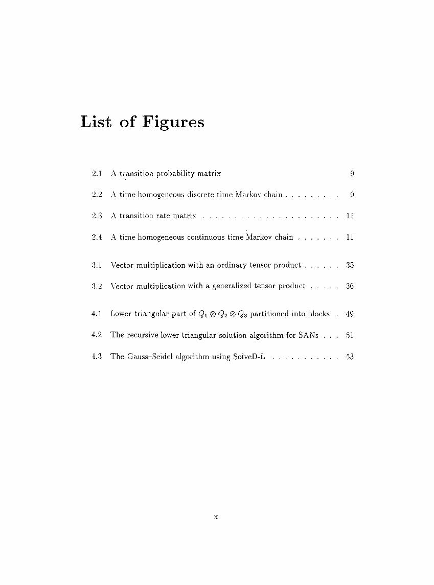
List of Figures
2.1 .A transition probability matrix 9
2.2 .A time homogeneous discrete time Markov chain..................... 9
2.3 .A transition rate m a tr ix ............................................................... 11
2.4 A time homogeneous continuous time Markov c h a in ............... 11
3.1 Vector multiplication with an ordinary tensor product............ 35
3.2 Vector multiplication with a generalized tensor p ro d u ct........ 36
4.1 Lower triangular part of Q\® Qz partitioned into blocks. . 49
4.2 The recursive lower triangular solution algorithm for SANs . . . 51
4.3 The Gaus,s-Seidel algorithm using S o lv e D -L ............................ 53
X
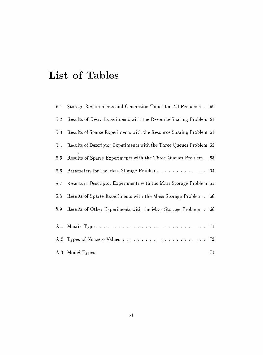
List of Tables
0.1 Storage Requirements and Generation Times for All Problems . .59
•0.2 Results of Desc. Experiments with the Resource Sharing Problem 61
■0.3 Results of Sparse Experiments with the Resource Sharing Problem 61
•0.4 Results of Descriptor Experiments with the Three Queues Problem 62
■0..0 Results of Sparse Experiments with the Three Queues Problem . 63
•0.6 Parameters for the Mass Storage Problem........................................64
•0.7 Results of Descriptor E.xperiments with the Mass Storage Problem 6-5
•5.8 Results of Sparse E.xperiments with the Mass Storage Problem . 66
•0.9 Results of Other Experiments with the Mass Storage Problem . 66
A .l Matrix Types
.A.2 Types of Nonzero V alues.................................................................... 72
•A.3 Model Types 74
XI
Chapter 1
Introduction
Markov chains [16] are one of tlie most widely' used modeling technic[ues in the scientific community. The range of application domains is wide, including natural sciences and engineering disciplines. The simple requirement for a system to be modeled as a Markov chain is that the system’s next action (transition) depend only on the current state of the system, named as the mtmoryless or the Markov property [16, p. 4]. Several natural phenomena that arise in biology, physics and chemistry can be modeled as Markov chains. In engineering sciences Markov chains have a wide use in several branches
of industrial engineering, electronics and computer engineering. Performance evaluation and reliability modeling is the field that Markov chains find the most use in computer engineering.
The random behavior of a system should posses a geometric or exponential probability distribution in order to be modeled as a Markov chain, since these are the only probability distributions that carry the memoryless property [16, p. 4]. Fortunately, the number of systems that show this structure is large and we have methods for fitting the random characteristics of most systems into e.xponential or geometric distributions.
After modeling a system as a Markov chain, one seeks quantitative information from the built model. One attractive feature of Markov chain models is that most interesting properties of a Markov model can be obtained by solving
CHAPTER 1. INTRODUCTION
a linear system of equations. Much research result is available concerning the numerical solution of Markov chain models. In addition to this, interest in this field of research is still alive. Most methods for solving systems of linear equations may be used for Markov chain models effectively. Direct methodsdo not seem to be suitable for solving large and sparse systems which arise in/Markov chain models. Several types of iterative methods are applied to Markov chains and their properties in the context of Markov chain models are studied. However, much research needs to be done, for understanding the behavior of iterative methods, especially non-stationary iterative methods like GMRES and .Arnoldi[8].
In Markov chain applications, the problem size increases very quickly as the applications get more interesting. This problem is referred to as the state space explosion[lQ, 14, 4] problem and has initiated different approaches to the Markov chain problem. .Approximate solutions and bounds for the solution vector[14] are studied for reducing the complexity of the problem. In plain words the coefficient matrix, constructed for solving the linear system of equations, becomes very large and prohibits one to solve interesting problems beyond a certain limit. Stochastic Automata Networks (SANs) [16. 10. 11] are developed to overcome the difficulties that accompany the state space explosion problem. Although it is possible to apply SAN methodology to different domains, performance modeling of parallel and distributed computer systems are especially suited to this type of approach[5j. In SAN methodology, a system is modeled as a set of components interacting with each other. Characteristics of each component is captured separately from the interactions among the components, and formulated in compact form, which leads to considerable reduction in the amount of storage needed for the model. Methods available for solving Markov chain problems obtained from a SAN formalism, appear in two forms. One might prefer to store the coefficient matrix of the linear system of equations in sparse format. However, this approach does not make use of the storage reduction provided by the SAN methodology. On the other hand, it is possible to solve the system by only referring to the compact storage of the model. Currently, the power method and non-stationary methods of GMRES and Arnoldi are implemented for SANs in compact form, but there are no results available concerning the solution of a real life problem obtained from
CHAPTER 1. INTRODUCTION
these methods[17, 6].
In this thesis, we introduce the concept of a splitting for a SAN in compact form and develop the stationary methods of Jacobi, Gauss-Seidel and SOR based on this splitting[16, 7]. We also implement these iterative methods based on splittings and their block versions. In addition to this, we e.xperiment with these methods on real life problems. We investigate the performance of these methods and their sparse counterparts compared to the power method.
In the following chapter, we introduce several concepts related to Markov chains and give the formulation of the problem of solving a Markov chain model as a linear system of equations. Stationary methods for Markov chain problems are also introduced in this chapter.
The third chapter discusses SANs. The concept of a SAN model in compact form is e.xplained with an example and the necessary algebraic framework for building SAN models is also provided. This chapter ends with an algorithm and a theorem regarding the complexity of the algorithm, that proves to be useful for SAN models in compact form.
The stationary iterative methods based on splittings for solving S.ANs in compact form are introduced in the following chapter. The algorithms provided for the methods are explained and a section on numerical results present the performance of the methods on three problems. Some interesting properties of block methods that have gone unnoticed so far are included in this chapter. An upper bound on the number of multiplications for the Gauss-Seidel and SOR methods are derived at the end of the chapter.
The last chapter contains conclusive remarks about the methods investigated. Observations and comments about methods, the SAN methodology and Markov chains based on our work are provided in the chapter.
We included an appendix that describes how to incorporate new models into the Peps package[12], which is the software tool developed in France for
solving S.AN models in compact form, since we implemented our methods as an extension to Peps.
Chapter 2
Markov Chains
2.1 Preliminaries
In our attempt to understand the characteristics of natural and artificial phenomena. mathematical models of systems are developed. It is possible to build models using the concept of the system being in a number of states. Generally, the system is thought to be in an initial state, and its behavior is modeled as transitions from one state to another. It is also possible to classify systems according to certain properties they might hold. One such property that the system modeled as a process changing states might have is the memoryless property, i.e., it only remembers its current state [16, p. 4]. In other words, the system’s transition from one state to the other is independent from the previous states that the system has visited.
In many of the models arising from diverse fields including natural sciences such as physics and biology, and engineering sciences such as industrial, electrical and computer engineering, the system either has or can be modeled as having memoryless property [16, p. 3]. The systems that posses the memoryless property may be modeled as a Markov process [16, p. 4].
A system modeled as a Markov process has a number of possible states. The actual number of possible states can be infinite, however the system can be at only one of the possible states at any time instant [16, p. 4]. In addition
to this, it is assumed that the transition time, the time it takes the system to go from one state to the other is negligible. That is, the transitions are said to take place instantaneously. [16, p. 3]
It is possible to have a continuous state space for a Markov process. For instance, if the output voltage of an electric circuitry can take all values within a range, and if the system can be modeled as a Markov process, it can be modeled as a Markov process with a continuous state space, having the output voltage as states of the system. If, for instance, the circuitry’s output voltage raises from 0.6 volts to 3.7 volts, one would view the model as making a transition from state 0.6 to state 3.7. On the other hand, if the output voltage can take only certain potential values, and if the system can be modeled as a Markov process, the system can be modeled as a discrete state space Markov process. Note that the actual values of the voltages do not effect the discrete or continuous character of the system.
Markov processes with discrete state spaces are called Markov chains [16, p. 5], and they are what our work is based on.
In the ne.xt section, we give the definition of a Markov chain in a formal con- te.xt. The following two sections introduce two different types of Markov chains that arise in Markov chain modeling. Stationary distribution of a Markov chain[16. p. 15] is an important quantity for determining certain characteristics of the model under consideration, and is introduced in the ne.xt section. Finally, methods developed for solving Markov chain models are discussed in the last section.
CHAPTER 2. MARKOV CHAINS 5
2.2 Formal Definition of Markov Chains
.A. Markov chain is a special case of a Markov process and, a Markov process is a stochastic process satisfying certain requirements. Hence, we give the definitions of stochastic processes in general, then Markov processes and Markov
chains based on this.
Definition 2.2.1 [16, p. 4] A stochastic process is defined as a family of random variables { X { t ) , t G T } defined on a given probability space indexed by the index parameter t, where t varies over some index set (parameter space) T.
In general, t takes values from the range (—oo ,+ co ). In applications, the index set T is thought of as the set of time points at which observation about the system is made. In other words, the index t of the random variable is defined as the time point that X{t) takes the observed value. In such cases, t takes values from the range [0,+oo). Depending on the characteristics of the values t takes, the process is either a continuous parameter (time) stochastic process or a discrete parameter (time) stochastic process. If i can take discrete values only, or similarly, if obser^■ation about the system is made only certain equidistant time points, the process is called a discrete-time parameter process. If the range of values of t is [0, +cxo) without any restrictions, or the system is observed at time points that are not equidistant, the process is referred to as a continuous-time stochastic process.
D efinition 2.2.2 Markov property: [16. p. 4] Let {X{ t ) , t G T } be a stochastic process defined on a given probability space indexed by the time index parameter t. where t varies over time index set T. Let the system be observed at time points to, t i . , . . . ,tn and let to < ti < . . . < The stochastic process {A’ (f), i G T } is said to have the Markov property if and only if
Prob{X{t) < x\X{to) = Xo,A'(ii) = X i,. .., .Y (i„ ) = ;i-„}
= Prob{X{t) < a;|A (i„) = x „}.
CHAPTER 2. MARKOV CHAINS 6
In plain words, Markov property states that the next transition of the system from the current state X{tn) = Xn to the next state X{t) = x, depends only on the current state X{tn) = Xn and is independent of its previous state history, i.e., it is independent of the states A’(io) = 2:0, A ’(ti) = x \ ,... ,X (t „_ i) = .r„_i. In other words, the current state of the process provides sufficient information to make the next transition.
D efinition 2.2.3 A Markov process is a stochastic process which satisfies the Alarkov property.
For any stochastic process, and hence for any Markov process, the values that the random variables X{t) take, define the state space of the process. As with the index set parameter t, the state space of a process can be continuous or discrete, finite or infinite.
D efinition 2.2.4 .4 Markov chain is a Markov process whose state space is discrete.
CHAPTER 2. MARKOV CHAINS 7
In Markov chain terminology, the state space of a chain is generally associated with the set of natural numbers. In other words the states are referred as state 0. state 1. etc.
When a stochastic process possesses a certain condition on the random variables and the index parameter (namely the Markov property), the process is said to be a Markov process. Similarly, the time index set and the state space characteristics of a Markov chain give rise to several types of Markov chains.
In a homogeneous Markov chain, the transitions of the system are independent of the time parameter t. The Markov property requires that the next transition be independent of the previous state history of the process. However, it is possible that the proce.ss makes a transition which is dependent both on the current state of the system and the value of the time parameter t. Such a Markov chain, in which the transitions out of a state are dependent on the time parameter i, is called a non-homogeneous Markov Chain.
Similar to the state space of the process, the index set (the time parameter) can be continuous or discrete. If the time parameter of a chain takes its values from a discrete set, the Markov chain is called a Discrete Time Markov Chain (DTMC). If the values of t are are continuous, the Markov chain is called a
Continuous Time Markov Chain (CTMC).
In summary, there are four parameters that describe a stochastic process. First, the continuous or discrete character of the state space, is a determining property of the process. Second, the continuous or discrete character of the time parameter introduce another classification dimension for the processes. Third,
the time homogeneity of the process, is also an important quantity, in capturing the properties of a process. Finally, the characteristics of the relations between the index set and and the random variables, i.e., the dependencies among them, define classes of stochastic processes. The classification that is determined by the character of the state space is important and is discussed in more detail in the following chapters.
2.3 Discrete Time Markov Chains
CHAPTER 2. MARKOV CHAINS 8
If the index set of the Markov chain is countable, i.e., it is in one to one correspondence with the set of natural numbers, the Markov chain is called a Discrete Time Markov Chain. In this case, the index set is in general taken to be the set of natural numbers and the random variables are numbered accordingly, i.e., as -Yo, A 'l,. . . , A „.
For a non-homogeneous Discrete Time Markov chain, the Markov property is described as [16, p. 5]
Prob{ An+i ^ ^n+i IAq .I’oi A j — X i , A . j i — Xn}
Prob{ A ti.)-! ^ Xn-j-ilAji — ·
The conditional probability that the process makes a transition to a new state j , given that it is in current state i, is called the single step transition probability. It is expressed as [16, p. 5]
Pij{n) = Prob{A',t+i =j\Xn = i}.
Note that since the Markov chain is a Discrete Time Markov chain, the state indices i and j are natural numbers.
For a homogeneous Markov chain, the next transition of the process is independent of the index parameter n. The single step transition probabilities are written as
Pij ~ Prob{A,i-t-l ~ ~ }·
The random variables A’„ should be geometrically distributed in order to satisfy the Markov property. In other words there is no other discrete probability
CHAPTER 2. MARKOV CHAINS
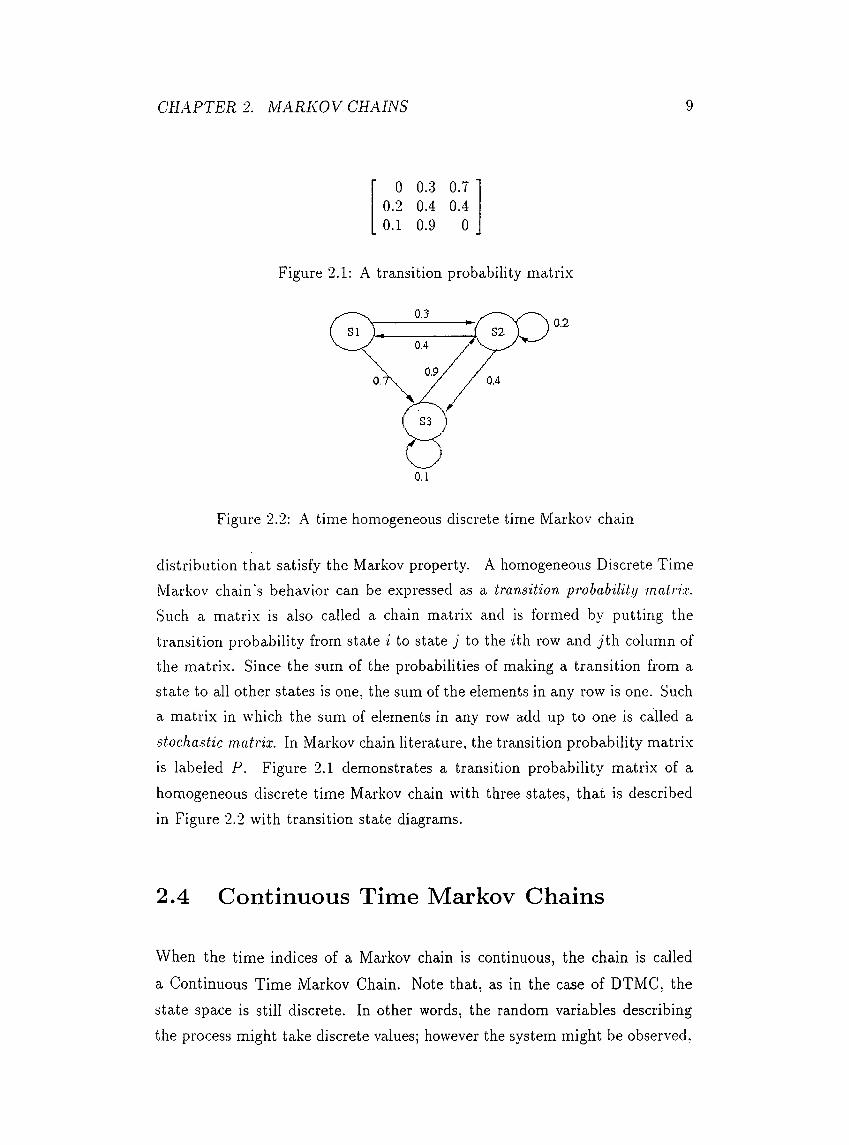
0 0.3 0.70.2 0.4 0.40.1 0.9 0
Figure 2.1: A transition probability matrix
0.2
Figure 2.2: A time homogeneous discrete time Markov chain
distribution that satisfy the Markov property. A homogeneous Discrete Time Markov chain's behavior can be e.xpressed as a transition probability matrix. Such a matrix is also called a chain matrix and is formed by putting the transition probability from state i to state j to the ith row and jth column of the matrix. Since the sum of the probabilities of making a transition from a state to all other states is one, the sum of the elements in any row is one. Such a matrix in which the sum of elements in any row add up to one is called a stochastic matrix. In Markov chain literature, the transition probability matrix is labeled P. Figure 2.1 demonstrates a transition probability matri.x of a homogeneous discrete time Markov chain with three states, that is described in Figure 2.2 with transition state diagrams.
2.4 Continuous Time Markov Chains
When the time indices of a Markov chain is continuous, the chain is called
a Continuous Time Markov Chain. Note that, as in the case of DTMC, the state space is still discrete. In other words, the random variables describing the process might take discrete values; however the system might be observed,
CHAPTER 2. MARKOV CHAINS 10
i.e., make transitions, at any instant in time.
The Markov property for a non-homogeneous Continuous Time Markov Chain is expressed as [16, p. 17]
Prob{A '(i„+i) < Xn+i \ X{to) = xo,X{t i ) = X u · . . ,X ( i „ ) = Xn}
= Prob{A'(i) < x\X{tn) =
for any sequence of time points to < t\ < . . . < tn < tn+i-
The transition probability of a non-homogeneous CTMC is given by
= Prob{A '(0 = j\X{s) = ?}, for t > s.
Ill the homogeneous case, since the probabilities are independent of the actual values of s and t, the transition probability is expressed in terms of the difference t = {t — s), i.e.,
p,j(r) = Prob{X(s + r) = i|A'(s) = i}.
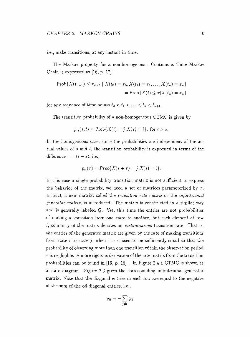
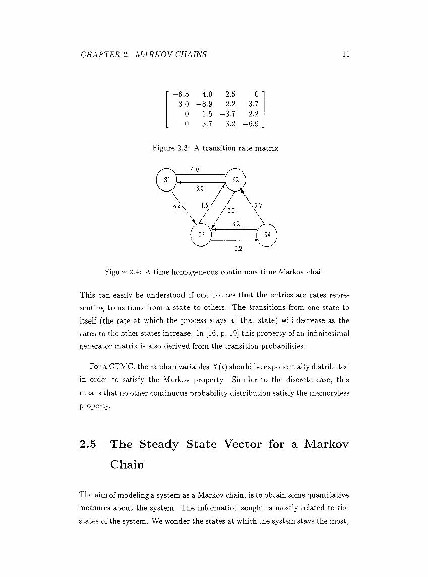
Ill this case a single probability transition matrix is not sufficient to express the behavior of the matrix, we need a set of matrices parameterized by r. Instead, a new matrix, called the transition rate matrix or the infinitesimal generator matrix, is introduced. The matrix is constructed in a similar way and is generally labeled Q. Yet, this time the enfries are not probabilities of making a transition from one state to another, but each element at row i, column j of the matrix denotes an instantaneous transition rate. That is, the entries of the generator matri.x are given by the rate of making transitions from state i to state j , when r is chosen to be sufficiently small so that the probability of observing more than one transition within the observation period T is negligible. .A. more rigorous derivation of the rate matrix from the transition probabilities can be found in [16. p. 18]. In Figure 2.4 a CTMC is shown as
a state diagram. Figure 2.3 gives the corresponding infinitesimal generator matrix. Note that the diagonal entries in each row are equal to the negative of the sum of the off-diagonal entries, i.e.,
<?í¡ = ~ Qij-
CHAPTER 2. MARKOV CHAINS 11
—6.5 4.0 2.5 03.0 -8 .9 2.2 3.7
0 1.5 -3 .7 2.20 3.7 3.2 -6 .9
Figure 2.3; A transition rate matrix
Figure 2.4: A time homogeneous continuous time Markov chain
This can easily be understood if one notices that the entries are rates representing transitions from a state to others. The transitions from one state to itself (the rate at which the process stays at that state) will decrease as the rates to the other states increase. In [16. p. 19] this property of an infinitesimal generator matrix is also derived from the transition probabilities.
For a CTMC. the random variables X{t) should be exponentially distributed in order to satisfy the Markov property. Similar to the discrete case, this means that no other continuous probability distribution satisfy the memoryless property.
2.5 The Steady State Vector for a Markov
Chain
The aim of modeling a system as a Markov chain, is to obtain some quantitative measures about the system. The information sought is mostly related to the states of the system. We wonder the states at which the system stays the most.
CHAPTER 2. MARKOV CHAINS 12
how long the system occupies certain states in the long run, etc. Depending on the system being modeled, one might be interested in some states of the system more than the others. Also, in general, the states of a Markov chain are classified into several groups and determining to which group a state belongs might be of interest, see [16, p. 8]. Specifically, a transient state is one which the system might not return back, in the long run. A recurrent state is one which the system is guaranteed to return after a number of transitions. In a Markov chain, it is possible that the process makes a transition to one state, and can not leave that state, i.e., there are transitions to that state but there are not any transitions out of the state. Such states are referred to as absorbing states. In practice, one is more interested in states that have some desirable or undesirable properties. Thus, one might wonder the probabilities of being ¿it those states or the average time the system spends at those states, in the long run.
It is suitable to express the state of a Markov model as a probability vector. A row vector tt is used with each entry i denoting the probability of being at state i. When the system’s behavior is captured as a transition rate matrix Q or a transition probability matrix P, the properties of the Markov chain can be expressed as a simple set of linear ecpiations.
Now we introduce two important quantities that have desirable properties in the sense that they answer or provide the necessary information to answer several questions sought from a Markov chain model.
D efinition 2.5.1 Limiting Distribution of a DTAIC :[16, p. 15] Given an ini
tial probability distribution 7t(0), if the limit
lim 7r(n)n—*co
exists, then this limit is called the limiting distribution, and we write
7T = lim 7r(n)
D efinition 2.5.2 Limiting Distribution of a CTMC iGiven an initial proba
bility distribution 7t(0), if the limit
lim irit)t—x>
CHAPTER 2. MARKOV CHAINS 13
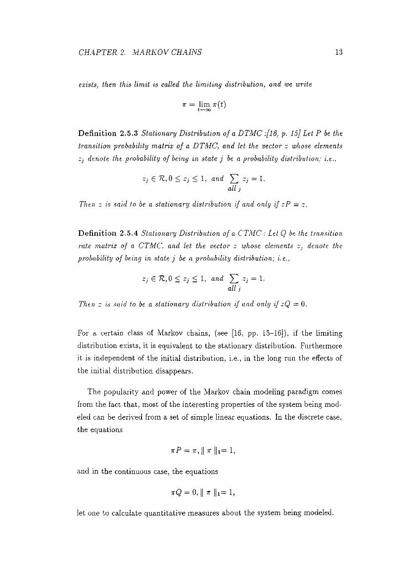
exists, then this limit is called the limiting distribution, and -we write
7T = lim 7r(i)f—CO '
D efinition 2.5.3 Stationary Distribution of a DTMC :[16, p. 15] Let P be the transition probability matrix of a DTAIC, and let the vector z whose elements Zj denote the probability of being in state j be a probability distribution; i.e.,
G ^ Zj ^ 1, and 'y ' Zj = 1.all j
Then z is said to be a stationary distribution if and only if zP — z.
Definition 2.5.4 Stationary Distribution of a CTMC : Let Q be the transition rate matrix of a CTMC. and let the vector z whose elements Zj denote the probability of being in state j be a probability distribution; i.e.,
Zj G 7 , 0 < < 1, and ^ = 1.all j
Then z is said to be a stationary distribution if and only if zQ = 0.
For a certain class of Markov chains, (see [16, pp. 15-16]), if the limiting distribution exists, it is equivalent to the stationary distribution. Furthermore it is independent of the initial distribution, i.e., in the long run the effects of the initial distribution disappears.
The popularity and power of the Markov chain modeling paradigm comes from the fact that, most of the interesting properties of the system being modeled can be derived from a set of simple linear equations. In the discrete case, the equations
wP = 7T, II 7T ||i= 1,
and in the continuous case, the equations
t Q = 0, II 7t ||i= 1,
let one to calculate quantitative measures about the system being modeled.
CHAPTER 2. MARKOV CHAINS 14
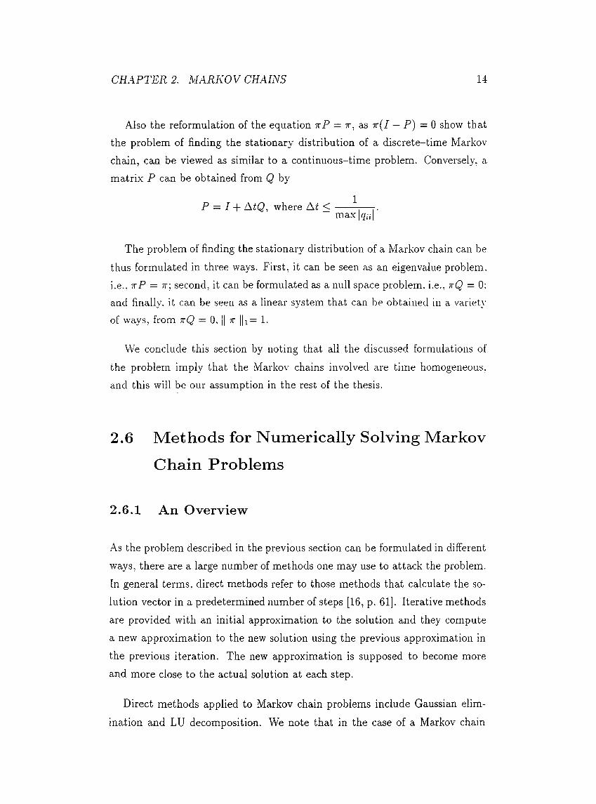
Also the reformulation of the equation ttP = tt, as 7t( J — P) = 0 show that the problem of finding the stationary distribution of a discrete-time Markov chain, can be viewed as similar to a continuous-time problem. Conversely, a matrix P can be obtained from Q by
1P = / + AtQ, where At <max I g,·,· I
The problem of finding the stationary distribution of a Markov chain can be thus formulated in three ways. First, it can be seen as an eigenvalue problem, i.e., 7tP = 7t; second, it can be formulated as a null space problem, i.e., kQ = 0: and finally, it can be seen as a linear system that can be obtained in a variet\· of ways, from ~Q = 0, || tt ||i = 1.
VVe conclude this section by noting that all the discussed formulations of the problem imply that the Markov chains involved are time homogeneous, and this will be our assumption in the rest of the thesis.
2.6 Methods for Numerically Solving Markov Chain Problems
2.6.1 An Overview
-As the problem described in the previous section can be formulated in different ways, there are a large number of methods one may use to attack the problem. In general terms, direct methods refer to those methods that calculate the solution vector in a predetermined number of steps [16, p. 61]. Iterative methods are provided with an initial approximation to the solution and they compute a new approximation to the new solution using the previous approximation in the previous iteration. The new approximation is supposed to become more and more close to the actual solution at each step.
Direct methods applied to Markov chain problems include Gaussian elimination and LU decomposition. We note that in the case of a Markov chain
CHAPTER 2. MARKOV CHAINS 15
problem, a nontrivial solution other than the zero vector, to the system wQ = 0 is always available since it can be verified that Q is singular [16, p. 71].
Iterative methods can be grouped into two. First group of methods referred to as stationary methods include the power method, the method of Jacobi, the method of Gauss-Seidel and Successive Overrelaxation (SOR). The second group of methods are non-stationary methods, also referred to as Krylov subspace methods, include the method of Arnold!, Generalized Minimum Residual Method (GMRES) and the full orthogonalization method [16, pp. 117-230], [13]. In this work we concentrate on stationary iterative methods. Here we first give a comparison of direct and iterative methods in the conte.xt of Markov chains [16, pp. 61-62].
The value of a Markov chain model increases as the system being modeled becomes more and more complex. The increase in the complexity of the model is generally reflected as an increase in the number of the states of the Markov- model. This phenomenon is referred to as the state-space explosion problem. The increase in the number of states results in an increase in the size of the generator matrix. Beyond a certain limit, it becomes necessary to use a sparse storage scheme for storing the infinitesimal generator matrix. In addition to this, the matrices arising in Markov chain models are sparse, i.e., they contain only a few entries in each row. It is basically because of this reason that direct methods are considered disadvantageous, when compared to iterative solution techniques. Direct methods usually involve introducing new nonzero elements (fill-ins) into the matrix during factorization, which makes them inefficient and diflficult to deal with. Also, beyond a certain limit, especially for large problems, it might not be possible to store the newly altered matrix in core memory. In contrast, iterative methods involve only matrix-vector multiplications or equivalent operations, which do not alter the nonzero structure of the matrix. In addition to this, by not altering the matrix, we avoid the round-off errors which are observed in direct methods.
In certain cases, it might not be necessary to compute the stationary vector of a Markov chain, to high accuracy. In such uses, iterative methods allow one to stop the computation at a predefined error term.
CHAPTER 2. MARKOV CHAINS 16
On the other hand, iterative methods are usually accompanied with a slow convergence rate to the solution. It is this reason that one may use a direct method for Markov chain problems whenever the method is not limited im- practically by memory constraints. However, iterative methods ai'e still the dominant choice, unless a practically implementable direct method gives the solution in less time.
Stationary methods have been the subject of much research. Although the non-stationary methods seem promising, much research needs to be done on their convergence properties and to predict the number of iterations recjuired to find the solution of a problem. In the following sections we introduce the power method, method of .Jacobi, Gauss-Seidel and SOR.
2.6.2 Power Method
The power method is used to find the right-hand eigenvector of an ordinary matri.x corresponding to a dominant eigenvalue of the matrix. Thus, when the Markov chain problem is formulated as one of an eigenvalue problem, i.e., irP = 7T, power method might be used to solve the problem. Let the initial probability distribution among the states of a Markov chain be 7t(0), and let the probability transition matrix of the same chain be P. Then after the process makes a transition, (at the next step), the probability distribution becomes At the second step the probability distribution becomes7t(2) _ 7r(i)/3 = Tr °'>P' . At the step, the probability distribution is found by TrP’l = Note that, is the new approximation to the solutionat step k. For certain classes of Markov chains [16, p. 16], the vector tt**·'! approaches to the stationary distribution, i.e.,
lim = 7T, where tt --- ttP.k—roo
Power method is multiplying the approximation at each iteration by the probability transition matrix P, to obtain a new approximation. The convergence
of power method is in general slow. Further properties of the method in the
context of Markov chains can be found in [16, pp. 121-125].
CHAPTER 2. MARKOV CHAINS 17
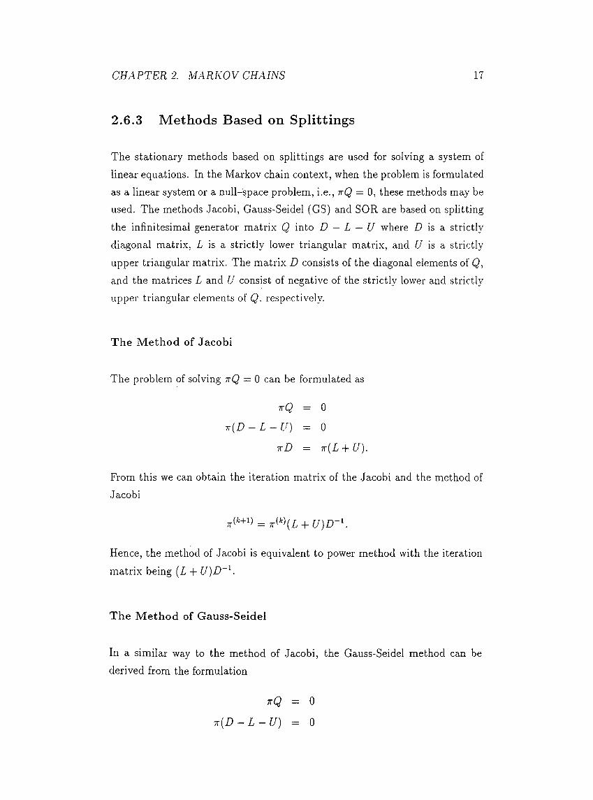
2.6.3 Methods Based on Splittings
The stationary methods based on splittings are used for solving a system of linear equations. In the Markov chain context, when the problem is formulated as a linear system or a null-space problem, i.e., ttQ = 0, these methods may be used. The methods .Jacobi, Gauss-Seidel (GS) and SOR are based on splitting the infinitesimal generator matrix Q into D — L — U where D is a, strictly diagonal matrix, T is a strictly lower triangular matrix, and U is a strictly upper triangular matrix. The matrix D consists of the diagonal elements of Q, and the matrices L and U consist of negative of the strictly lower and strictly upper triangular elements of Q. respectively.
The Method of Jacobi
The problem of .solving nQ = 0 can be formulated as
t Q = 0
k{ D - L - U ) = 0
ttD = Tr{L + U).
From this we can obtain the iteration matri.x of the Jacobi and the method of Jacobi
Hence, the method of Jacobi is equivalent to power method with the iteration matrix being (L + U)D~^.
The Method of Gauss-Seidel
In a similar way to the method of Jacobi, the Gauss-Seidel method can be derived from the formulation
ttQ = 0
: { D - L - U ) = 0
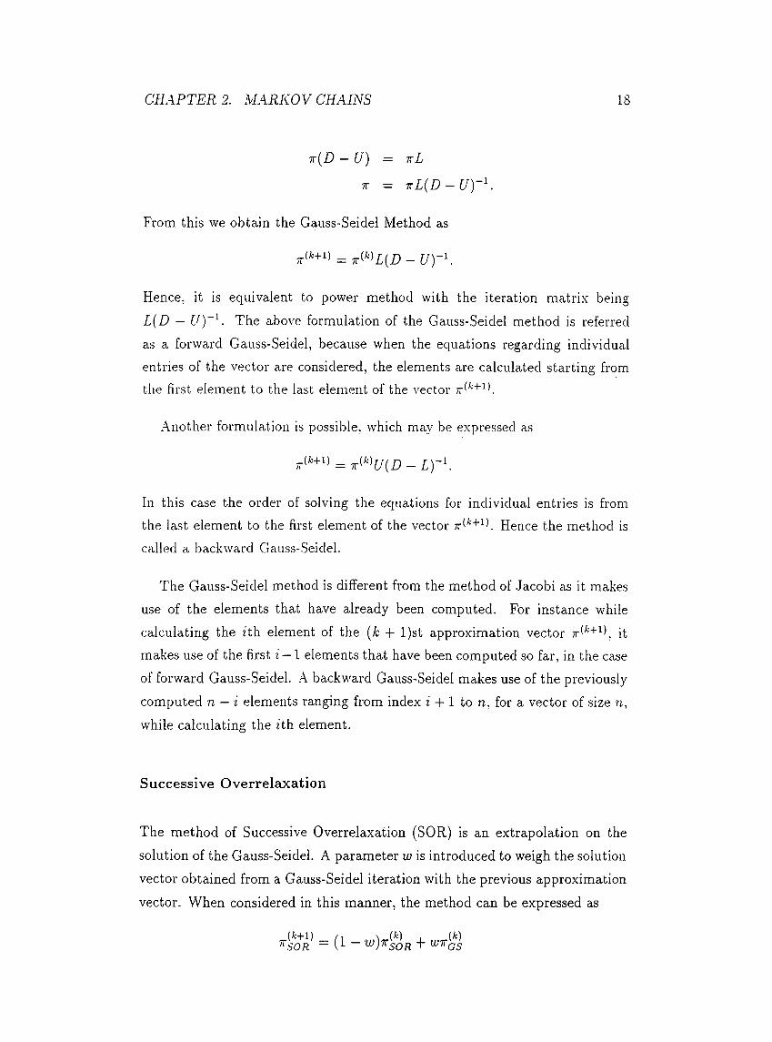
CHAPTER 2. MARKOV CHAINS 18
t { D - U ) = ttL
7T = ttL { D - U ) - K
From this we obtain the Gauss-Seidel Method as
Hence, it is eciuivalent to power method with the iteration matrix being L(D — U)~^. The above formulation of the Gauss-Seidel method is referred as a forward Gauss-Seidel, because when the equations regarding individual entries of the vector are considered, the elements are calculated starting from the first element to the last element of the vector
Another formulation is possible, which may be expressed as
In this case the order ol solving the equations for individual entries is from the last element to the first element of the vector ttG'+i ). Hence the method is called a backward Gauss-Seidel.
The Gauss-Seidel method is different from the method of Jacobi as it makes use of the elements that have already been computed. For instance while calculating the ith element of the [k + l)st approximation vector itmakes use of the first ¿ — 1 elements that have been computed so far, in the case of forward Gauss-Seidel. .A backward Gauss-Seidel makes use of the previously computed n — i elements ranging from index f -|- 1 to n, for a vector of size n, while calculating the ¿th element.
Successive Overrelaxation
The method of Successive Overrelaxation (SOR) is an extrapolation on the solution of the Gauss-Seidel. A parameter w is introduced to weigh the solution vector obtained from a Gauss-Seidel iteration with the previous approximation vector. When considered in this manner, the method can be expressed as
^SOR “ (1 ~ '^VSOR +
CHAPTER 2. MARKOV CHAINS 19
where is the resulting vector after applying the Gauss-Seidel algorithm to the ¿th approximation vector of SOR. Note that SOR is also called a forward SOR when the Gauss-Seidel iteration involved is a forward Gauss-Seidel, and a backward SOR when the Gauss-Seidel iteration involved is a backward Gauss- Seidel.
Hence forward SOR in matrix notation is
(A:+l) ^ (1 - -t-U;(7r'^U (r> - L)~^),
and backward SOR in matrix notation IS
Note that an SOR iteration with lu = 1 is equivalent to a Gauss-Seidel iteration. Sometimes SOR. is referred as Successive Under Relaxation method when0 < IÜ < 1.
In addition to forward and backward versions of SOR, a Symmetric SOR (SSOR) hcis been introduced, which is simply a forward SOR followed by a backward SOR. In the case of Markov chain problems, there is little benefit in using a SSOR instead of SOR and this can be observed only in rare examples [16, p. 132].
Convergence characteristics of stationary methods in a general context can be found in [7] and references therein. In the Markov chain context, [16, pp. 133-176], [4, pp. 125-132] and [1, pp. 26-28] [16, pp. 138-142] provide discussions of these and other methods.
Block Versions of Iterative Methods Based on Splittings
Stationary block iterative methods are based on block partitioning of the generator matrix Q. Following [16, p. 139] we can demonstrate a block partitioning
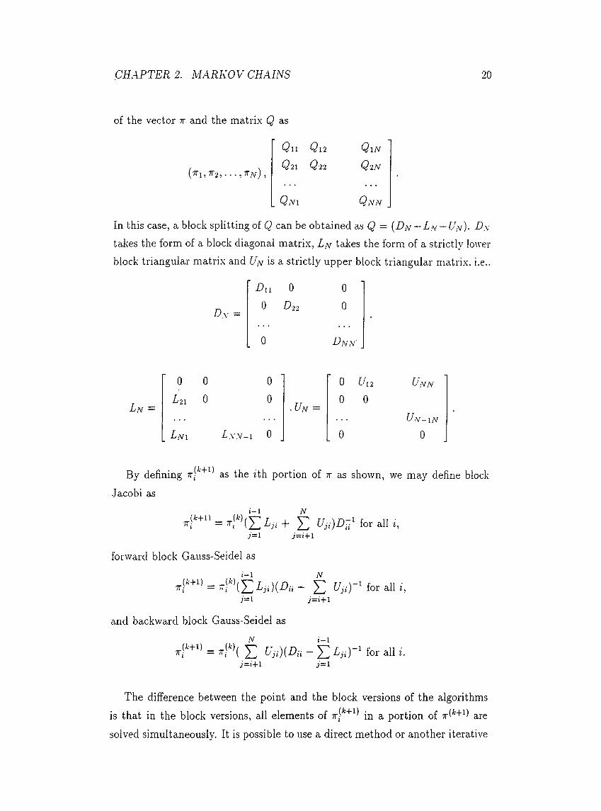
CHAPTER 2. MARKOV CHAINS 20
of the vector tt and the matrix Q as
(tTi , 7T2, · · · ? yv) )
Qll Qi2 Qin
Q21 Q22 Q2N
Qni Qnn
In this case, a block splitting of Q can be obtained as Q = (D¡^ — — D\
takes the form of a block diagonal matrix, L¡\r takes the form of a strictly lower block triangular matrix and I7/v is a strictly upper block triangular matrix, i.e..
D x =
Dn 0 00 D22 0
0
0 0 0 0 Uv2 Lxx
Lx = Lzi 0 0• Lx =
0 0Hx-ix
Lxi L.xv-i 0 0 0
By defining as the ith portion of tt as shown, we may define blockJacobi as
„p + ll ^ ^j= l j = ! + l
forward block Gauss-Seidel as
.G+l) _N
x r “ = -, E for alH.i = l j=i+l
and backward block Gauss-Seidel asN i-1
7Tp+‘ l = E í-'iúiDu - E i r i ) · ' for- all i.j=i+l i = l
The difference between the point and the block versions of the algorithms is that in the block versions, all elements of in a portion of aresolved simultaneously. It is possible to use a direct method or another iterative

CHAPTER 2. MARKOV CHAINS 21
method to solve the individual blocks. In this way, one can obtain a more accurate approximation at each iteration, obviously with an extra cost being introduced at each iteration. In [1 , pp. 26-28] block iterative methods are discussed within the context of Markov chains.
Chapter 3
Stochastic Automata Networks
3.1 Preliminaries
In the previous chapter we have seen that if a Markov chain model of a system is available, qiuintitative measures about the system can be obtained from the system of equations
ttQ = 0, II ;r ||i= 1.
There are a number of methodologies for developing a Markov chain model of a system. Petri nets [8] are such a formalism for generating Markov chain models of systems. Alternatively, there are special software tools for generating Markov chain models [15]. Independent of the paradigm used, the problem of state-space e.xplosion is observed in almost all applications. In some cases, as the applications become more interesting, the size of the Markov chain gets so large that it is impractical to find a solution.
A Stochastic Automata Network (SAN) is another formalism for generating
a Markov model. They are most suitable for performance modeling of parallel and distributed systems. The model is generated by considering an individual automaton for each component of the system. Each individual component is modeled by a single stochastic automaton and the interactions between the components are incorporated into the model. The main advantage of the SAN
99
CHAPTER 3. STOCHASTIC AUTOMATA NETWORKS 23
methodology is that the model is stored very efficiently, i.e., the memory occupied by the model is very small compared to the size of the model generated.
Before getting into the formal definitions of SANs and their properties, we give a basic overview of tensor algebra which is a building block for SAN methodology.
3.2 Tensor Algebra
3.2.1 Ordinary Tensor Algebra
We now list several definitions regarding tensor algebra. These and morere properties of tensor algebra concepts can be found in [2].
In the following, we use Amxn for a matrix of dimension m x n, B t for a matrix of dimension k x 1. Cmkxni and Dmkxni for matrices of size mk x nl.
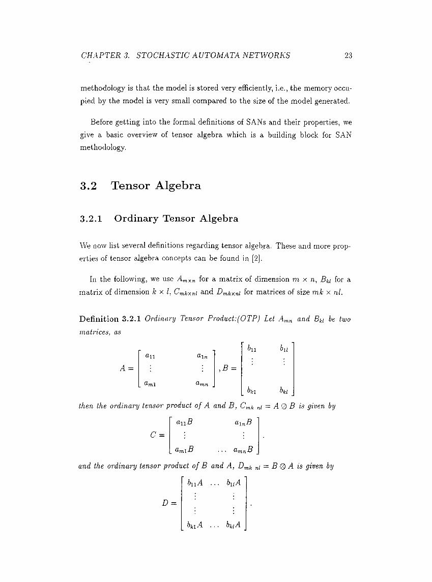
D efinition 3.2.1 Ordinary Tensor Product:(OTP) Let A„i„ and Bki he two matrices, as
h\\ b\i
A =
an Ir,B =
hki hki
then the ordinary tensor product of A and B , Cmk ni = A Q B is given by
aiiB o-inB
c = \ ;
^ml-B . . . a mnB
and the ordinary tensor product of B and A, Dmk ni = B 0 A is given by
h\\A . . . hiiA
D = '
hki A ·■■ bkiA
CHAPTER 3. STOCHASTIC AUTOMATA NETWORKS 24
Notice that C ^ D.
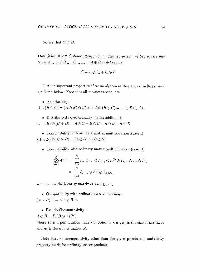
D efin ition 3.2.2 Ordinanj Tensor Sum: The tensor sum of two square ma- trzcei> A.JIJ2. nncl EjTiTTij Ctjiyji, titti — A. B zs defined us
C = A ® I m + I n
Further important properties of tensor algebra as they appear in [5, pp. 4-5] are listed below. Note that all matrices are square.
• Associativity ;
.4 0 {B 0 C) = {A 0 B) 0 C) and .4 0 (B 0 C) = (.4 0 .B) 0 C).
• Distributivity over ordinary matri.x addition :
(.4 + B ) 0 {C + D) = A 0 C + B 0 C + A 0 D + B e D.
• Compatibility with ordinary matrix multiplication :(case I)(.4 X B ) 0 {C X D) = { A 0 C) X {B 0 D).
• Compatibility with ordinary matrix multiplication :(case II)
N
(g) = n «1 ® ® n._. 0 0 0 . . . 0 /,¿=1 ¿=1
N
= n 0 AS' 0 /¿ + 1;/V,¿=1
where Ii-j is the identity matrix of size Y[i=ink·
• Compatibility with ordinary matrix inversion :(A X = 4 - 1 0 B ~ \
• Pseudo Commutativity :
A 0 B = Pr{B 0 A)P^,
where Pr is a permutation matrix of order Ui x U2, nj is the size of matrix A and rin is the size of matrix B.
Note that no commutativity other than the given pseudo commutativity property holds for ordinary tensor products.
CHAPTER 3. STOCHASTIC AUTOMATA NETWORKS 25
It is straightforward to extend these properties to N term tensor products and sums. For our purpose of illustrating several algorithms, noting that
N N(g) ^ 0 . . . 0 0 A ^ 0 0 . . . 0k = l k = l
where /„^ is defined to be the identity matrix of size Uk which is the size of theterm of the ten.sor product , A K is sufficient.
3.2.2 Generalized Tensor Algebra
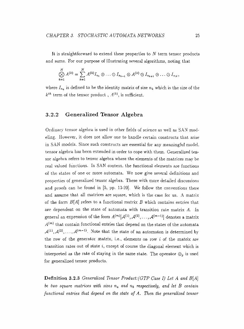
Ordinary tensor algebra is used in other Helds of science as well as SAN modeling. However, it does not allow one to handle certain constructs that arise in S.AN models. Since such constructs are essential for any meaningful model, tensor algebra has been extended in order to cope with them. Generalized tensor algebra refers to tensor algebra where the elements of the matrices may be real valued functions. In SAN context, the functional elements are functions of the states of one or more automata. We now give several definitions and properties of generalized tensor algebra. These with more detailed discussions and proofs can be found in [5, pp. 13-20]. VVe follow the conventions there and assume that all matrices are square, which is the case for us. A matrix of the form B[A] refers to a functional matrix B which contains entries that are dependent on the state of automata with transition rate matrix A. In general an expression of the form denotes a matrix
that contain functional entries that depend on the states of the automata . . . , Note that the state of an automaton is determined by
the row of the generator matrix, i.e.. elements on row i of the matrix are transition rates out of state i, except of course the diagonal element which is interpreted as the rate of staying in the same state. The operator 0 is used for generalized tensor products.
D efin ition 3.2.3 Generalized Tensor Product:(GTP Gase I) Let A and B[A\
he two square matrices with sizes and respectively, and let B contain functional entries that depend on the state of A. Then the generalized tensor
CHAPTER 3. STOCHASTIC AUTOMATA NETWORKS 26
product of A and B , C — A®g B[A] is given by
ацВ{аі) ai2B{ai)
a2lB(^a2 ) *22-^(^2)
Па1-®(^Па) Па2- ( По)
α ι„„β(αι)
α2πα^(«2)
^ПаПа і^Па )
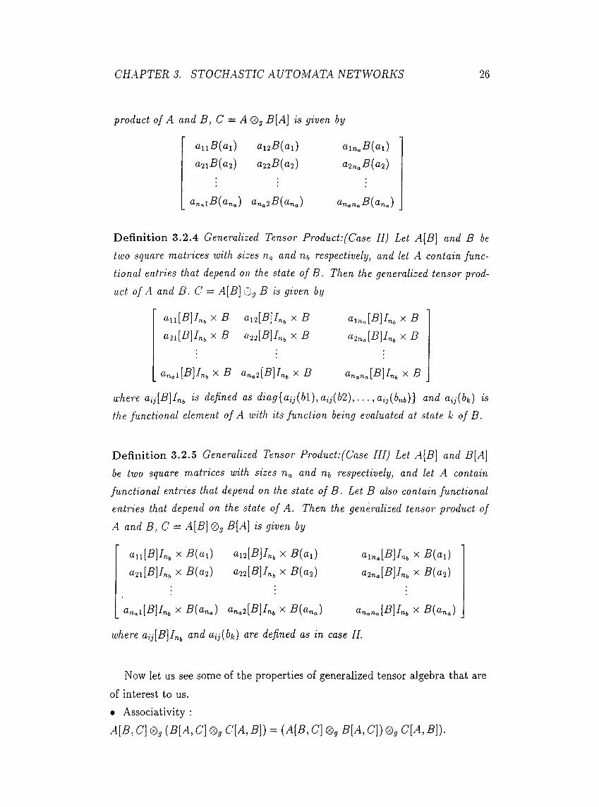
Definition 3.2.4 Generalized Tensor Product:(Case II) Let A[B] and B be two square matrices with sizes n, and ni, respectively, and let A contain func
tional entries that depend on the state of B . Then the generalized tensor prod
uct of A and B . C = A[B] Ag B is given by
ап[В]Іпь X B ar¿[B]Inb x B U2i[B]Inb X B а22[В]Іпь X B
аіпа[В]Іпь X B - 'ína\B\In|, X B
^ ncil\B\Ini, X B ana2[- ]- il(, X B nanc\B\In,, X B
where aij[B\In is defined as diag{aij{bl),aij{b2 ) , . . . ,aij(bnb)} and aij{bk) is the functional element of A with its function being evaluated at state k of B.
Definition 3.2.5 Generalized Tensor Product:(Case III) Let A[B] and B[A] be two square matrices with sizes Па and щ respectively, and let A contain functional entries that depend on the state of B. Let B also contain functional entries that depend on the state of A. Then the generalized tensor product of A and B, C = A[B\ 0 g B[A] is given by
ап[В]Іщ X B(ai) au[B]Kt, x B{ai) й2і[В]Іщ X B{a2) а22[В]Іщ x B{a2)
^^lna[B]In^, X В{^йі)
а2па[В]Іпь X В{а2)
0'Паі\.В\Ігц, X В{апа) ^Па2[В]Іп(, X В{^СІп ) ^^nana\B\In , X Bi^ünf)
where aij[B]I^ and aij{bk) are defined as in case II.
Now let us see some of the properties of generalized tensor algebra that are
of interest to us.• Associativity :A[B, C] 0g (B[A, C] ®g C[A, B]) = {A[B, C] 0g B[A, C]) 0g C[A, B]).
CHAPTER 3. STOCHASTIC AUTOMATA NETWORKS 27
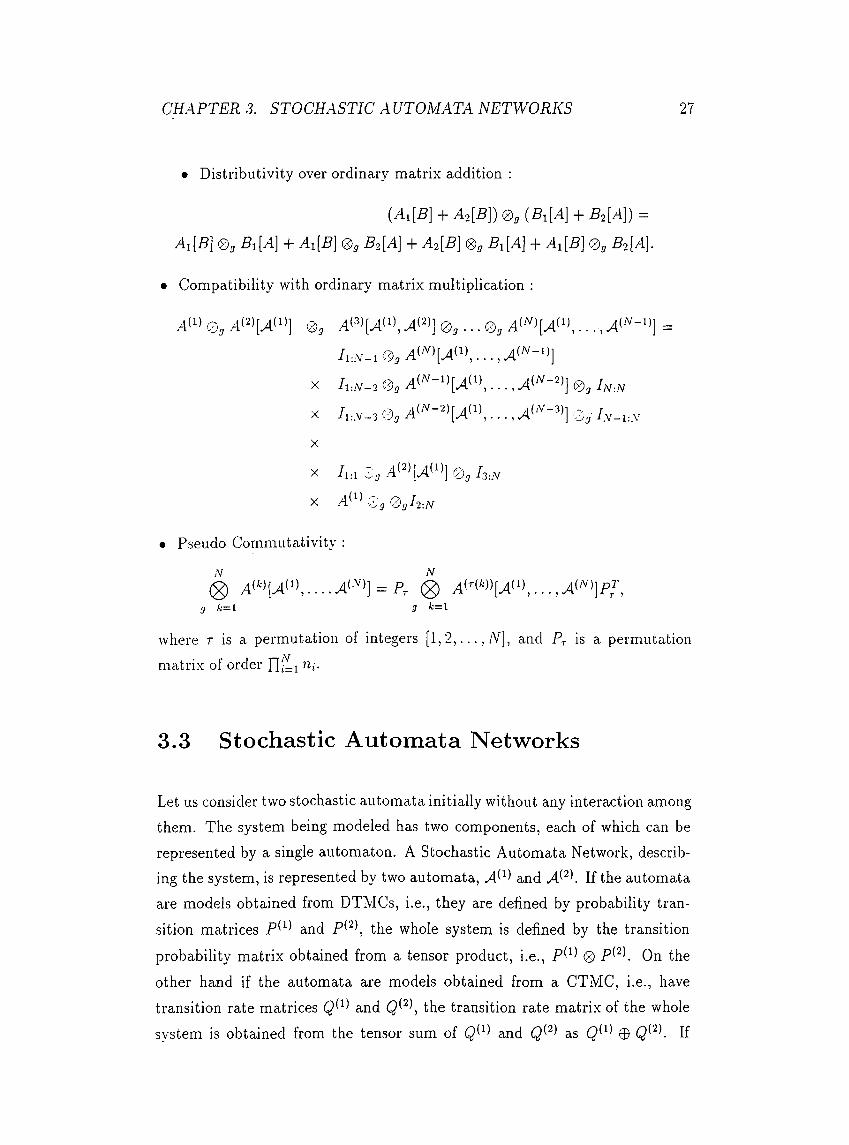
• Distributivity over ordinary matrix addition :
(Ai[5] + Ao[B]) 0 , {B,[A\ + B2[A]) =
A\[B\ ®g -6l[A] + A\[B] ®g + ^2[-5] ®g B\[A\ + A\[B] 0g B2\A\.
Compatibility with ordinary matrix multiplication :
0 , 0 , ^(2)] 0 , . . . 0 , . . . , >lbv-i)]
h : N - i ® g
I\:N--2 ®g A^ . . . , 0 j In:N
X /i:.V-3 0 , . . . , 0 ,
X
X h : l Zg A^^^[A^^^]0g K y
X .4^^* Zg Zgh- .N
• Pseudo Commutativity :
N N
j /l=1 9 ’=1
where r is a permutation of integers [1, 2, . . . , jV], and Pr is a permutation
matrix of order [li^i i·
3.3 Stochastic Automata Networks
Let us consider two stochastic automata initially without any interaction among them. The system being modeled has two components, each of which can be represented by a single automaton. A Stochastic Automata Network, describing the system, is represented by two automata, If the automataare models obtained from DTMCs, i.e., they are defined by probability tran
sition matrices P ^ and the whole system is defined by the transition
probability matrix obtained from a tensor product, i.e., © P ^ On theother hand if the automata are models obtained from a CTMC, i.e., have transition rate matrices and Q ' \ the transition rate matrix of the whole system is obtained from the tensor sum of and as If
CHAPTER 3. STOCHASTIC AUTOMATA NETWORKS 28
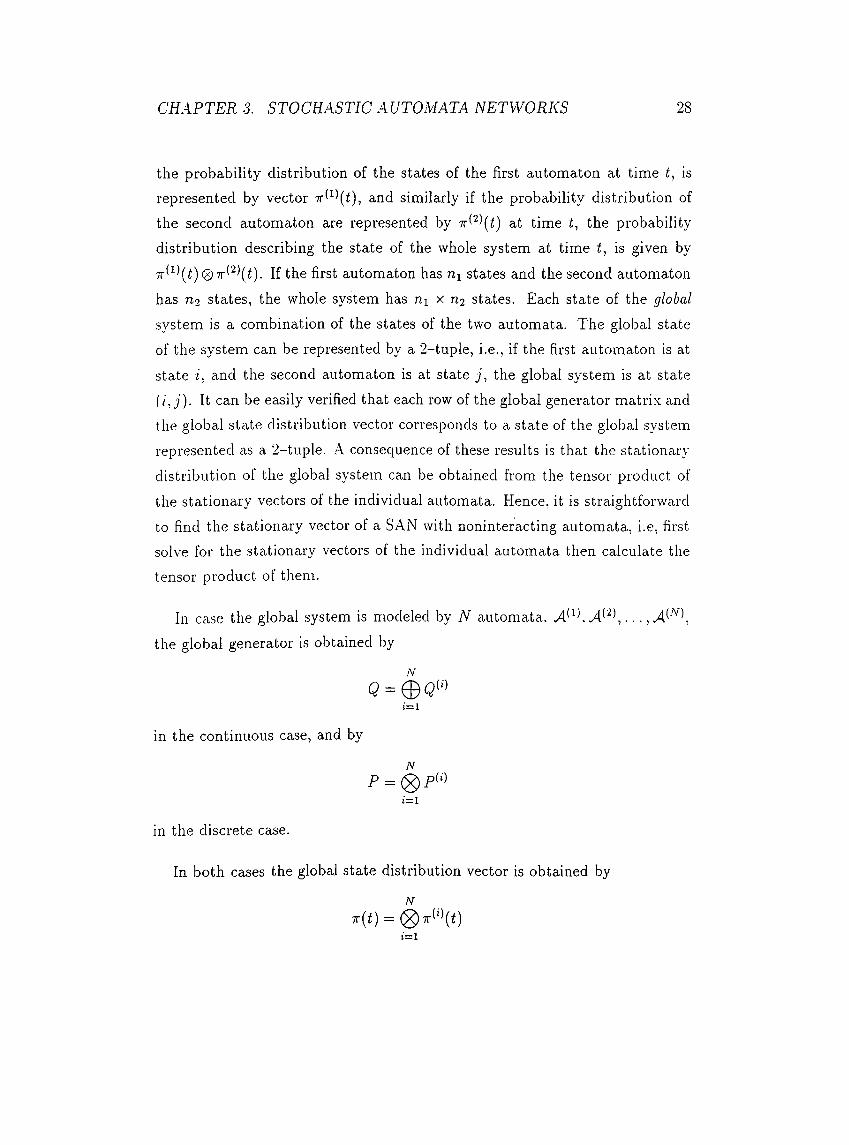
the probability distribution of the states of the first automaton at time i, is represented by vector 7r(^^(i), and similarly if the probability distribution of the second automaton are represented by 7г(^)(í) at time i, the probability distribution describing the state of the whole system at time t, is given by
0 7гf^^(í). If the first automaton has rii states and the second automaton has U2 states, the whole system has rii x ri2 states. Each state of the global system is a combination of the states of the two automata. The global state of the system can be represented by a 2-tuple, i.e., if the first automtiton is at state i. and the second automaton is at state j , the global system is at state (i. j)· It easily verified that each row of the global generator matri.x andthe global state distribution vector corresponds to a state of the global system represented as a 2-tuple. A consequence of these results is that the stationary distribution of the global system can be obtained from the tensor product of the stationary vectors of the individual automata. Hence, it is straightforward to find the stationary vector of a SAN with noninteracting automata, i.e, first solve for the stationary vectors of the individual automata then calculate the tensor product ol them.
In case the global system is modeled by N automata. the global generator is obtained by
N
0 = ©«''■>¿=1
in the continuous case, and by
P =t=l
in the discrete case.
In both cases the global state distribution vector is obtained by
7r(t) =¿=1
CHAPTER 3. STOCHASTIC AUTOMATA NETWORKS 29
3.4 Capturing the Interactions
3.4.1 Functional Transitions
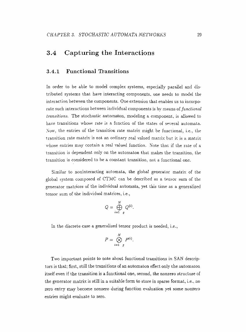
In order to be able to model complex systems, especially parallel and distributed systems that have interacting components, one needs to model the intei'ciction between the components. One extension that enables us to incorporate such interactions between individual components is by means of functional transitions. The stochastic automaton, modeling a component, is allowed to have transitions whose rate is a function of the states of several automata. Now, the entries of the transition rate matrix might be functional, i.e., the transition rate matrix is not an ordinary real valued matrix but it is a matrix whose entries may contain a real valued function. Note that if the rate of a transition is dependent only on the automaton that makes the transition, the transition is considered to be a constant transition, not a functional one.
Similar to noninteracting automata, the global generator matrix of the global system composed of CTiVtC can be described as a tensor sum of the generator matrices of the individual automata, yet this time as a generalized tensor sum of the individual matrices, i.e.,
<?= Фi'=l g
In the discrete case a generalized tensor product is needed, i.e.,
NP = p(i)
!=1 g
Two important points to note about functional transitions in SAN descriptors is that; first, still the transitions of an automaton effect only the automaton itself even if the transition is a functional one, second, the nonzero structure of the generator matrix is still in a suitable form to store in sparse format, i.e., no zero entry may become nonzero during function evaluation yet some nonzero
entries might evaluate to zero.
CHAPTER 3. STOCHASTIC AUTOMATA NETWORKS 30
3.4.2 Synchronizing Events
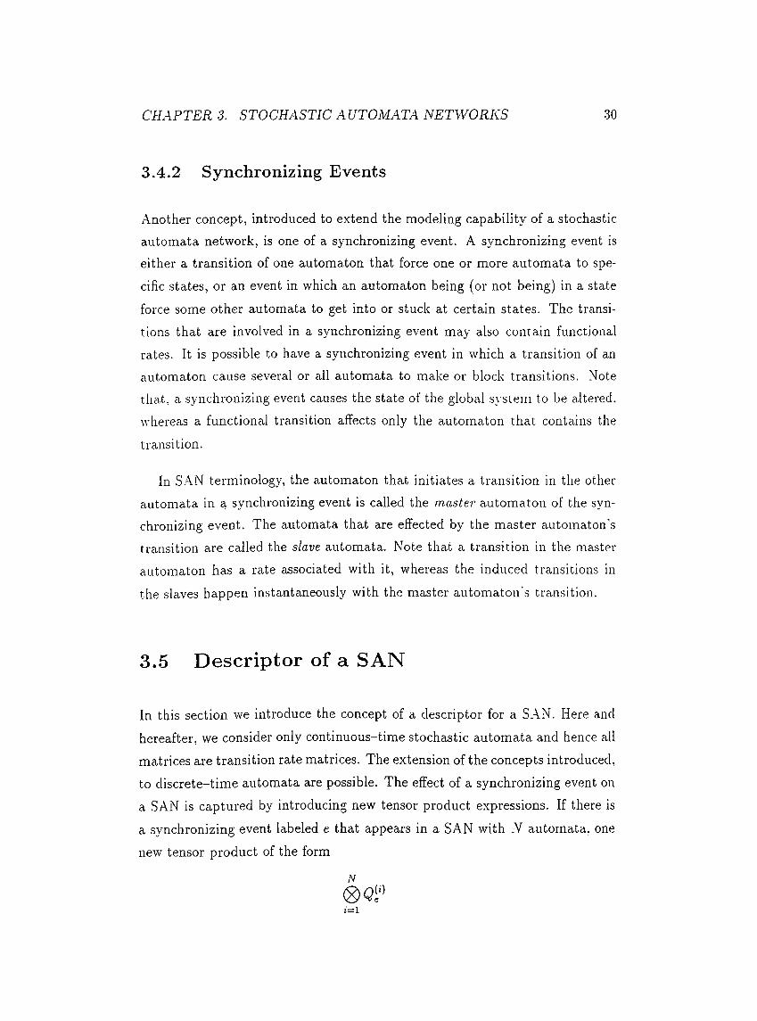
Another concept, introduced to extend the modeling capability of a stochastic automata network, is one of a synchronizing event. A synchronizing event is either a transition of one automaton that force one or more automata to specific states, or an event in which an automaton being (or not being) in a state force some other automata to get into or stuck at certain states. The transitions that are involved in a synchronizing event may also contain functional rates. It is possible to have a synchronizing event in which a transition of an automaton cause several or all automata to make or block transitions. Note that, a synchronizing event causes the state of the global system to be altered, whereas a functional transition affects only the automaton that contains the transition.
In .SAN terminology, the automaton that initiates a transition in the other automata in a synchronizing event is called the master automaton of the synchronizing event. The automata that are effected by the master automaton’s transition are called the slave automata. Note that a transition in the master automaton has a rate associated with it, whereas the induced transitions in the slaves happen instantaneously with the master automaton's trcinsition.
3.5 Descriptor of a SAN
In this section we introduce the concept of a descriptor for a SAN. Plere and hereafter, we consider only continuous-time stochastic automata and hence all matrices are transition rate matrices. The extension of the concepts introduced, to discrete-time automata are possible. The effect of a synchronizing event on a SAN is captured by introducing new tensor product expressions. If there is
a synchronizing event labeled e that appears in a SAN with N automata, one new tensor product of the form
N
1=10
CHAPTER 3. STOCHASTIC AUTOMATA NETWORKS 31
and another one in the form
0 Q i ‘ >2 = 1
are introduced. The last term is referred to as the diagonal corrector of the synchronizing event and is introduced to maintain the global generator as a transition rate matri.x:. In the most general case, where the transitions involved in the synchronizing event, say e,·, are functional, the tensor products are generalized tensor products and the expressions introduced are in the forms
¿=1
andN
■7 1=1
For a SAN model with N automata, there are N matrices in the tensor products, each of which correspond to one automaton in the SAN. For each synchronizing event, the order of the terms in each tensor product are explicit as described bv
and
Q i" 0 , 0 , . . . 0 , e r >
0 , Ql"’ 0 j . . . 0 j O f* .
This is important since neither ordinary nor generalized tensor products are commutative.
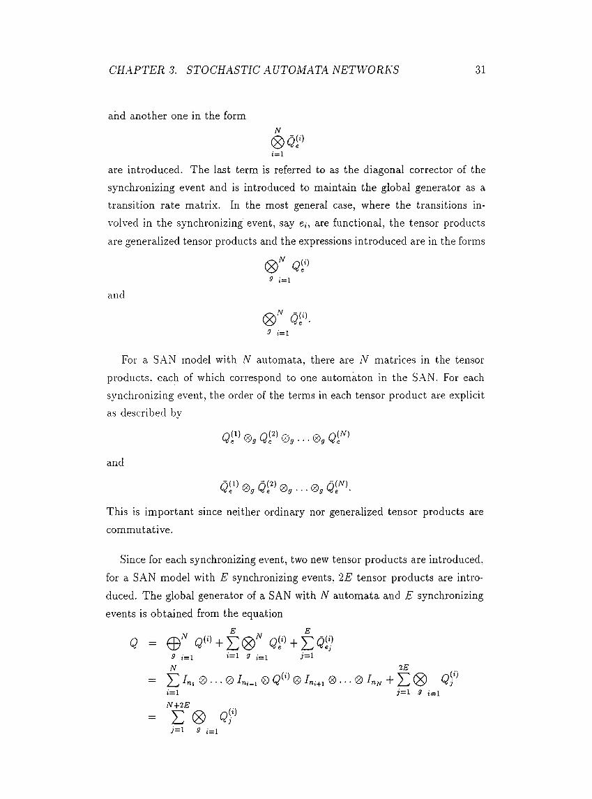
Since for each synchronizing event, two new tensor products are introduced, for a SAN model with E synchronizing events, 2E tensor products are introduced. The global generator of a SAN with iV automata and E synchronizing events is obtained from the equation
N ^ ^Q = © « « + E © Of+ E<J?
9 i=i 1=1 9 i=l j = lN 2E
= E -1 ® ® ^«.-1 ® ® ^".+11=1 N+2E
• · 0 iriN + ^ (g) Qj(¿)
= E ® <55J=1 9 i=i
CHAPTER 3. STOCHASTIC AUTOMATA NETWORKS 32
and the form of it as in the last line is referred to as the descriptor of the SAN. The first set of N tensor products are referred to as the local generator matrices, the E tensor products of the form are referred as the synchro-nizing event matrices, the final tensor products of the form J2 f - i g
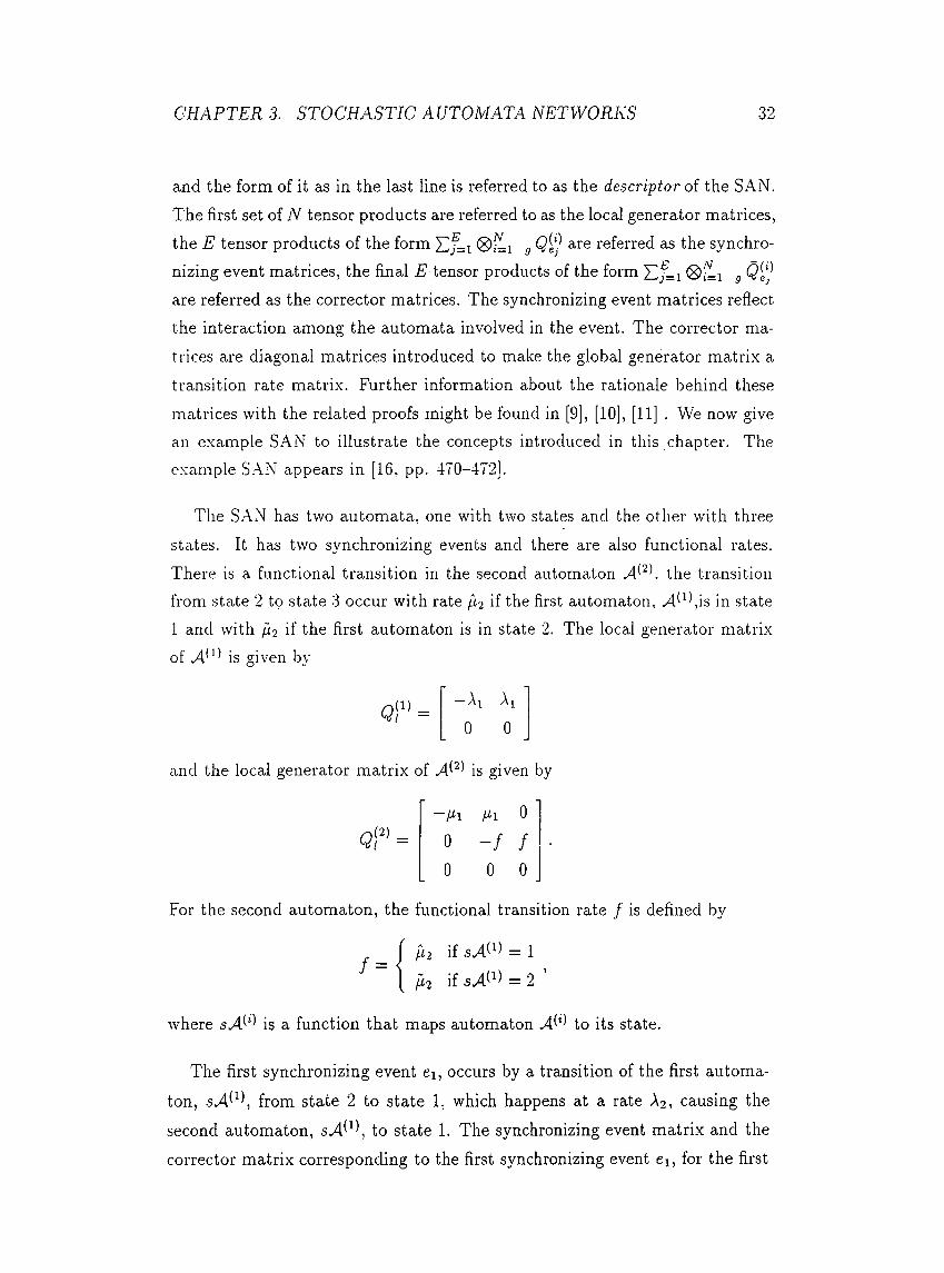
are referred as the corrector matrices. The synchronizing event matrices reflect the interaction among the automata involved in the event. The corrector matrices are diagonal matrices introduced to make the global generator matrix a transition rate matrix. Further information about the rationale behind these matrices with the related proofs might be found in [9], [10], [11] . We now give an example SAN to illustrate the concepts introduced in this chapter. The example SAN appears in [16, pp. 470-472].
The SAN has two automata, one with two states and the other with three states. It has two synchronizing events and there are also functional rates. There is a functional transition in the second automaton the transitionfrom state 2 to state 3 occur with rate /¿2 if the first automaton, ^^^l,is in state 1 and with ¡j.2 if the first automaton is in state 2. The local generator matrix of .4* * is given by
—Ai Ai0 0
- /A Ml 0
0 - / /0 0 0
and the local generator matrix of is given by
For the second automaton, the functional transition rate / is defined by
i ¡x-2 if = 1
I ¡i-2 if = 2
where is a function that maps automaton 4. ' to its state.
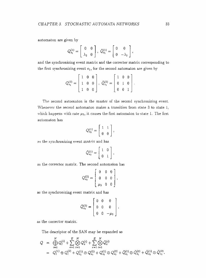
The first synchronizing event ei, occurs by a transition of the first automa
ton, from state 2 to state 1, which happens at a rate A2, causing thesecond automaton, to state 1. The synchronizing event matrix and thecorrector matrix corresponding to the first synchronizing event ei, for the first
CHAPTER 3. STOCHASTIC AUTOMATA NETWORKS 33
automaton are given by
oi:’ = 0 0
A2 0. 0 1 :’ =
0 0
0 — A 2
and the synchronizing event matrix and the corrector matrix corresponding to the first synchronizing event ei, for the second automaton are given by
Q ?N
’ 1 0 0 ' 1 0 0 , O' f =
' 1 0 0 ‘0 1 0
1 0 0 0 0 1
The second automaton is the master of the second synchronizing event. Whenever the second automaton makes a transition from state 3 to state 1. which happens with rate /H3 , it causes the first automaton to state 1. The firstautomaton has
1 1
0 0
as the synchronizing event matrix and has
1 0
0 1
as the corrector matrix. The second automaton has
' 0 0 0 ‘
= 0 0 0
_ /«3 0 0 _
as the synchronizing event matrix and has
' 0 0 0
Q^e^= 0 0 0
0 0 -pLz
as the corrector matrix.
The descriptor of the SAN may be expanded as
N E N E N
= ei" ® ei"+eii’ 0 eii’ + eii’ ® ei?+eii’ ® eif + eii’ 0 Q'S~
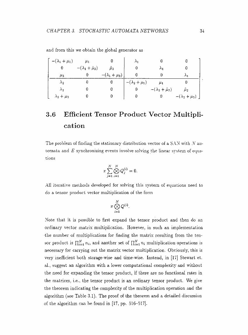
CHAPTER 3. STOCHASTIC AUTOMATA NETWORKS 34
and from this we obtain the global generator as
+ / J ' l ) Ml 0 Ai 0 00 - ( Ai + M2) M2 0 Ai 0
0 —(Ai + ^3) 0 0 Ai^ 2 0 0 -(A2 + Ml) Ml 0A 2 0 0 0 ~(A2 + M2) M2
A2 + A.3 0 0 0 0 - ( A2 + M3 )
3.6 Efficient Tensor Product Vector Multipli
cation
The problem of finding the stationary distribution vector of a SAN with N automata and E synchronizing events involve solving the linear system of equations
N N
i= l ¿=1
All iterative methods developed for solving this system of equations need to do a tensor product vector multiplication of the form
1=1
Note that it is possible to first expand the tensor product and then do an ordinary vector matrix multiplication. However, in such an implementation
■the number of multiplications for finding the matrix resulting from the tensor product is rii=i another set of [f ill multiplication operations isnecessary for carrying out the matrix vector multiplication. Obviously, this is very inefficient both storage-wise and time-wise. Instead, in [17] Stewart et. ah, suggest an algorithm with a lower computational complexity and without the need for expanding the tensor product, if there are no functional rates in
the matrices, i.e., the tensor product is an ordinary tensor product. We give the theorem indicating the complexity of the multiplication operation and the algorithm (see Table 3.1). The proof of the theorem and a detailed discussion of the algorithm can be found in [17, pp. 516-517].
CHAPTER 3. STOCHASTIC AUTOMATA NETWORKS 35
1. Initialize: nlef t = nin2 . . . n^v-i; nright = 1.2. For i = iV,. . . , 2,1 do
• base = T,jump = Ui x nright• For ¿ = 1, 2, . . . , n left do
o For j = 1 ,2 , . . . , nright do* index = base + j* For/ = 1 ,2 . . . . , Tii do
• •s/ = T index\ index - index + nright* Multiply: z — z X ■k index = base + j* For / = 1 ,2 , . . . , n,· do
■ i n d e x — index = index + nright o base = base + jump
• nleft = nleft frii^i• nright = nright x n,·• K = it'
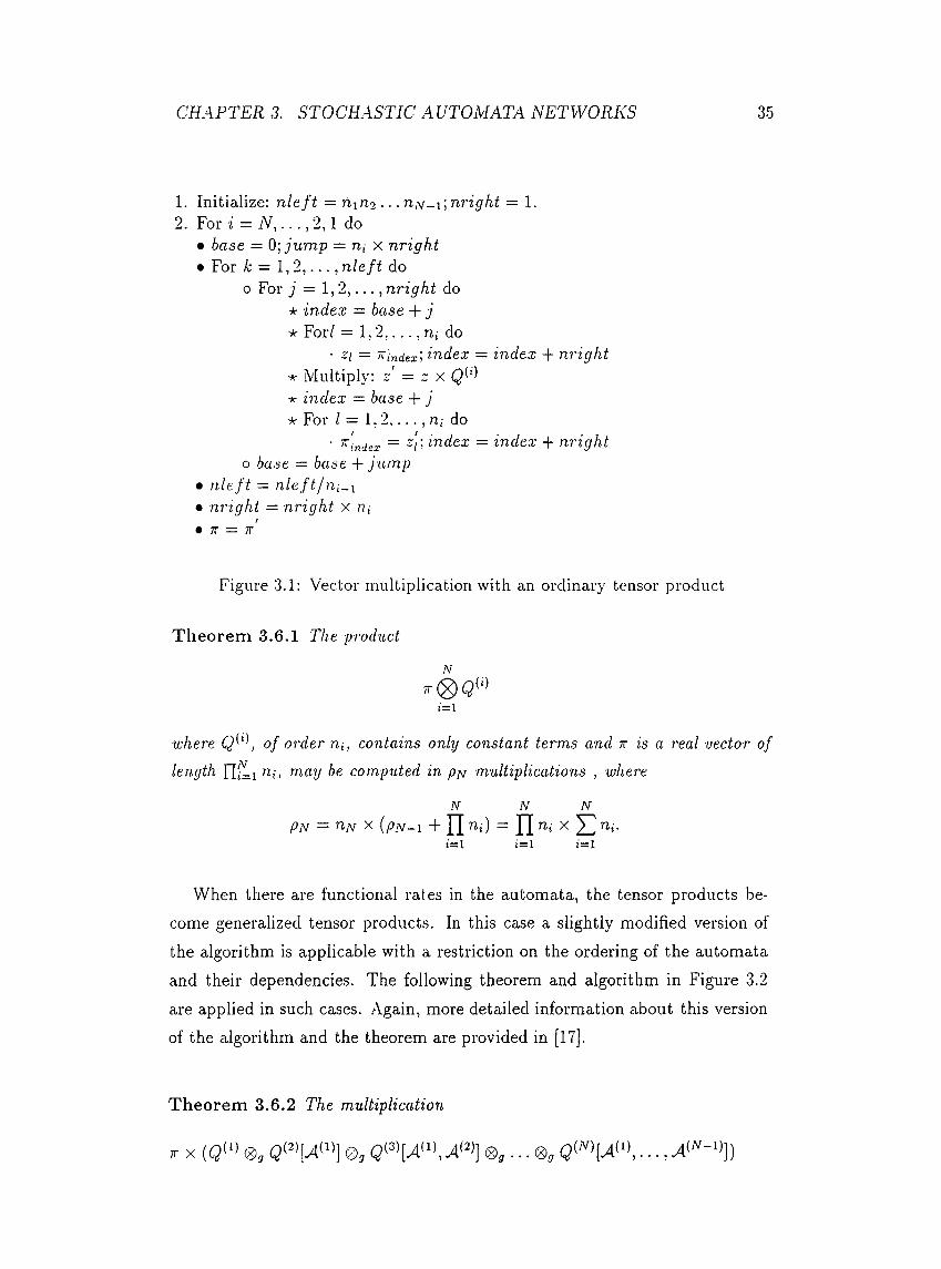
Figure 3.1: Vector multiplication with an ordinary tensor product
T h eorem 3.6.1 The product
1=1
where Q ‘\ of order ni, contains only constant terms and w is a real vector of length niay be computed in p/v multiplications , where
N N N
Pn = n.M X ( p i v - i + n = n ^ X !1=1 ¿=1 1=1
When there are functional rates in the automata, the tensor products become generalized tensor products. In this case a slightly modified version of the algorithm is applicable with a restriction on the ordering of the automata and their dependencies. The following theorem and algorithm in Figure 3.2
are applied in such cases. Again, more detailed information about this version of the algorithm and the theorem are provided in [17].
T h eorem 3 .6.2 The multiplication
X ((?<“' 0 , 0 , 0 , . . . 0 » . . . .
CHAPTER 3. STOCHASTIC AUTOMATA NETWORKS 36
1. Initialize: nlef t = nin? . . . n,v_i; nriqht = 1.2. For z = 7V,. . . , 2,1 do
• base = 0 ] jump = rii x nright• For ¿ = 1 ,2 , . . . , n le ft do
0 For _?’ = 1, 2 , . . . , i — 1 do* ¿j = ([(¿' - l ) / n 3 +i ni] mod (n|=i+i ni)) + 1
o For j = 1, 2, . . . , nright do★ index = base + j
Fold = 1 ,2 , . . . , n,· do• zi = ~index\ index = index + nright
-k Multiply: r' = ·: X . . . ,k index = base + j k For / = 1, 2 . . . . , n,· do
■ index ~ ~l'·· Mdtx — index + nright o base = base + jump
• nleft — nleft ftii-i• nright = nright x n,·
/• 7T = 7T
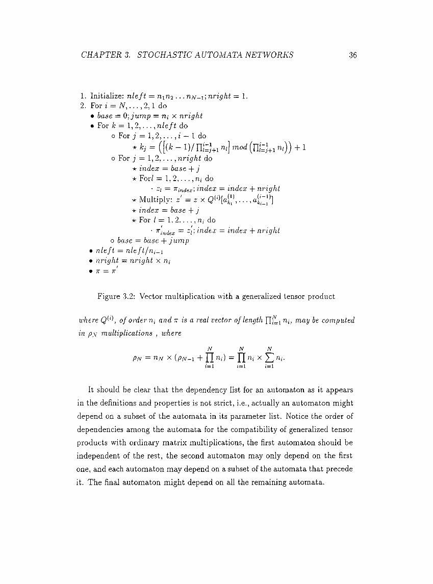
Figure 3.2: Vector multiplication with a generalized tensor product
where Q ‘\ of order ni and ~ is a real vector of length computed
in p s multiplications , where
N N N
PN - riM X [ p N - l + n " i) = n ^!=1 t= l (=1
It should be clear that the dependency list for an automaton as it appears in the definitions and properties is not strict, i.e., actually an automaton might depend on a subset of the automata in its parameter list. Notice the order of dependencies among the automata for the compatibility of generalized tensor products with ordinary matrix multiplications, the first automaton should be independent of the rest, the second automaton may only depend on the first one, and each automaton may depend on a subset of the automata that precede
it. The final automaton might depend on all the remaining automata.
Chapter 4
Stationary Iterative Methods for a SAN
4.1 The splitting of a SAN descriptor
111 order to use stationary iterative methods such as Jacobi, GS. and SOR for solving a SAN, the corresponding descriptor needs to be split. Here we give a suitable splitting for a SAN descriptor in the form D — L — U [16, p. 126]. By a suitable splitting we mean one in which L, D, and U each consists of a sum of tensor products so that iterative methods of interest may be implemented in terms of the efficient vector-tensor product multiplication algorithm.
The derivations of the splittings are based on the associativity of tensor products and distributivity of tensor product over matrix addition [2]. These two properties are valid for both OTP and GTP [5]. In other words, the splittings exist in both the nonfunctional (i.e., OTP) case and the functional (i.e., GTP) case. Obviously, limitations on the applicability of the efficient vector-descriptor multiplication algorithm still remain [5, pp. 13-24].
The descriptor of a SAN with N automata and E synchronizing events is
given by2E+N N
(1)2 E + A N
j=l i=l
37
CHAPTER 4. STATIONARY ITERATIVE METHODS FOR A SAN 38
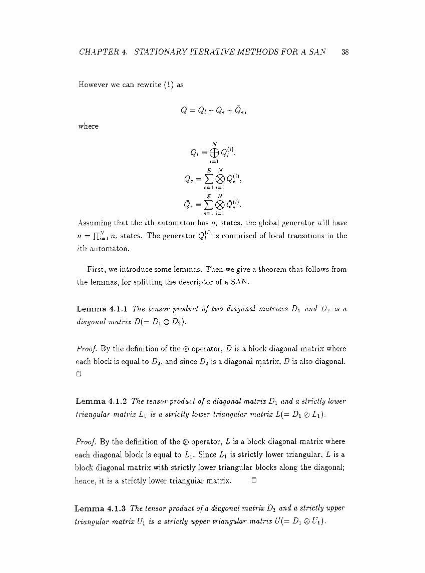
However we can rewrite ( 1) as
Q — Ql A Qe A Qei
where
N
0 / = © < ?,“ ’ .1=1
e= l ¿=1 E N _
0. =e= l i= l
Assuming that the ¿th automaton has ni states, the global generator will have
n = rii^i states. The generator <5/' is comprised of local transitions in the ¿th automaton.
First, we introduce some lemmas. Then we give a theorem that follows from the lemmas, for splitting the descriptor of a SAN.
L em m a 4.1.1 The tensor product of two diagonal matrices Di and Do is a diagonal matrix D {— D\ ® D 2 ).
Proof. By the definition of the 0 operator, D is a block diagonal matrix where each block is equal to D 2 , and since D2 is a diagonal matrix, D is also diagonal. □
L em m a 4.1.2 The tensor product of a diagonal matrix D\ and a strictly lower triangular matrix Li is a strictly lower triangular matrix L {— D\ © Li).
Proof. By the definition of the 0 operator, T is a block diagonal matrix where each diagonal block is equal to Ly. Since Li is strictly lower triangular, T is a block diagonal matrix with strictly lower triangular blocks along the diagonal;
hence, it is a strictly lower triangular matrix. □
L em m a 4 .1 . 3 The tensor product of a diagonal matrix D\ and a strictly upper triangular matrix Ui is a strictly upper triangular matrix U{= D i 0 Li).
CHAPTER 4. STATIONARY ITERATIVE METHODS EOR A SAN 39
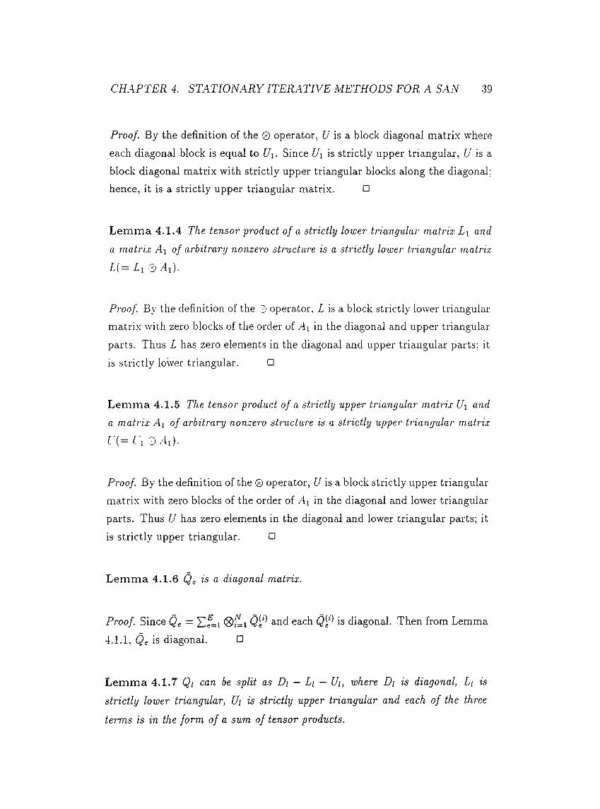
Proof. By the definition of the 0 operator, U is a block diagonal matrix where each diagonal block is equal to U\. Since U\ is strictly upper triangular, /7 is a block diagonal matrix with strictly upper triangular blocks along the diagonal; hence, it is a strictly upper triangular matrix. □
Lemma 4.1.4 The tensor product of a strictly lower triangular matrix L\ and a matrix A\ of arbitrary nonzero structure is a strictly lo wer triangular matrix
L { = L , 0 AC-
Proof. By the definition of the 0 operator, ¿ is a block strictly lower triangular matri.x with zero blocks of the order of _4i in the diagonal and upper triangular parts. Thus L has zero elements in the diagonal and upper triangular parts; it is strictly lower triangular. □
Lemma 4.1.5 The tensor product of a strictly upper triangular matrix U\ and a matrix Ai of arbitrary nonzero structure is a strictly upper triangular matrix
L (= f 1 0 .41).
Proof. By the definition of the 0 operator, 17 is a block strictly upper triangular matri.x with zero blocks of the order of A\ in the diagonal and lower triangular parts. Thus U has zero elements in the diagonal and lower triangular parts; it is strictly upper triangular. □
Lemma 4.1.6 Qg is a diagonal matrix.
Proof. Since Qe = Qi‘ ^ach is diagonal. Then from Lemma4.1.1, Qe is diagonal. □
Lemma 4.1.7 Q¡ can be split as Di — L¡ — Ui, where D¡ is diagonal, L¡ is strictly lower triangular, Ui is strictly upper triangular and each of the three
terms is in the form of a sum of tensor products.
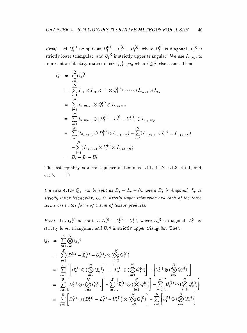
Proof. Let Q\‘'* be split as — U¡‘\ where is diagonal, isstrictly lower triangular, and is strictly upper triangular. We use Im-.nj, to represent an identity matrix of size n i—¿ i.· when i < j , else a one. Then
Qi = 0 ^/'^i=lN
CHAPTER 4. STATIONARY ITERATIVE METHODS FOR A SAN 40
= 0 I n ,0 - - - 0 Q r 0 · · · 0 0 Iny¿ = 1N
— Ini'.TLi-i 0 Ql 0 n¿ + i:n.v¿= 1
= E / . . .....¿ = 1
= o D\· 0 - [}p z :¿=1 ¿=1
N
¿■=1= Di — Li — Vi
The last equality is a consequence of Lemmas 4.1.1, 4.1.2. 4.1.3, 4.1.4, and 4.1.5. □
Lem m a 4.1.8 Qg can be split as Dg — Lg — Ug where Dg is diagonal. Lg is strictly lower triangular, Ug is strictly upper triangular and each of the three terms are in the form o f a sum of tensor products.
Proof. Let Q[‘'> be split as where is diagonal. L[‘ isstrictly lower triangular, and f/ 0 jg strictly upper triangular. Then
0 . = E ® « ?e=l ¿=1
e=l ¿=2E
= Ee=l L . E
= Ee=l L E
= Ee=l .
¿=2
Z )W ® (0 Q<·')i = 2
i = 2
-Ee=l
N
i < " 0 (0 C ? )i = 2
N
U¡'>0 (0 Qi‘ l)i = 2
r>i'> 0 0 ((® <?P )i = 3
E
-Ee=l L
E
-Ee=l L
1=2N
i = 2
CHAPTER 4. STATIONARY ITERATIVE METHODS FOR A SAN 41
- Ee = l L
E r
= Ee= l -
E
- Ee= l LE
- Ee = l .
1=3N
Di'>0 Di^>0 ( i ^ Q i ‘>){ = 3
N
i = 3
E r
- Ee= l
E
- Ee= l L
t=3
4 ‘’ 0(i|h3í‘’)1=2
N
i = 3
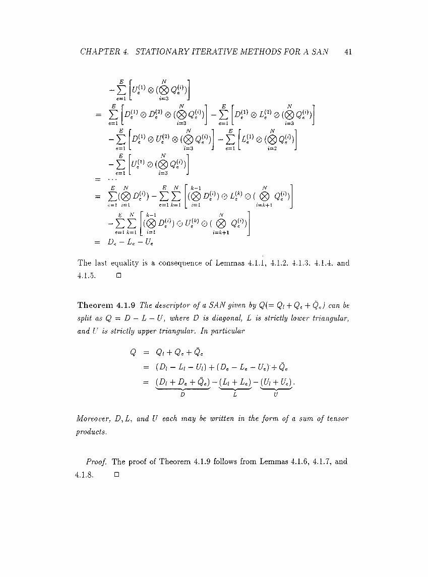
E N E N
= E « S ) " i ' ’ ) - E Ee=l^=1; = 1 i = l
£· yV- E E
e= l k=i
k-l N
(g) g ( ‘>)¿=i ¿ — /j 1
(S) OS'’ )1 = 1 z = A; +1
— y e — y e — Ue
The last equality is a consequence of Lemmas 4.1.1, 4.1.2. 4.1.S3. 4.1.4. and 4.1.5. □
T heorem 4.1.9 The descriptor o f a SAN given by Q (= Qi + + QN can he
split as Q = D — L — U, where D is diagonal, L is strictly lower triangular, and U is strictly upper triangular. In particular
Q — Qt A- Qe + Qe
= [Di - L i - Ui) + [D, - Le - U,y+
= [Di A De A Qe) — {Li A Lg) — {U¡ A Og) ■D U
Moreover, D,L, and U each may be written in the form of a sum of tensor products.
Proof. The proof of Theorem 4.1.9 follows from Lemmas 4.1.6, 4.1.7, and
4.1.8. □
CHAPTER 4. STATIONARY ITERATIVE METHODS FOR A SAN 42
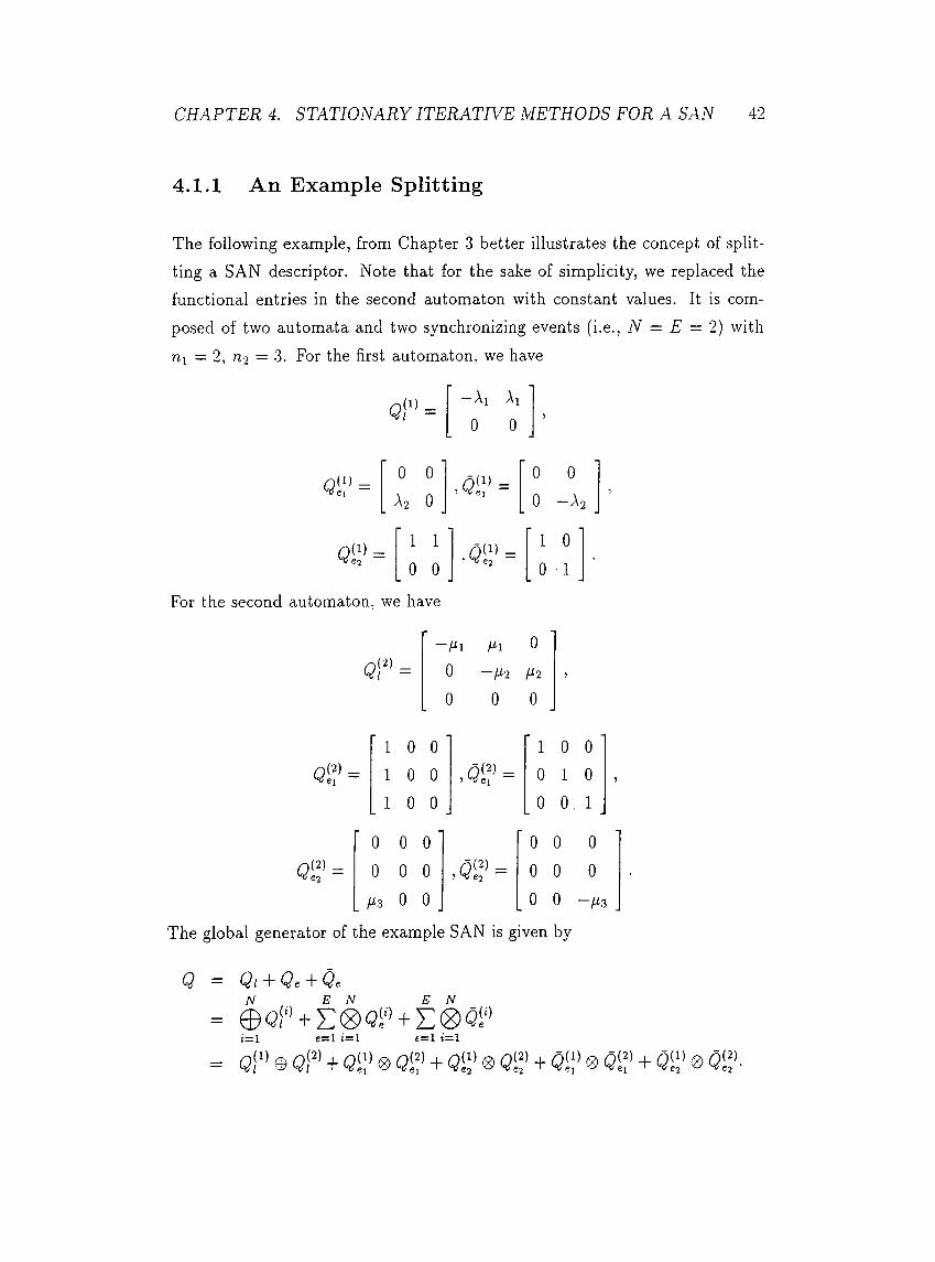
4.1.1 An Example Splitting
The following example, from Chapter 3 better illustrates the concept of splitting a SAN descriptor. Note that for the sake of simplicity, we replaced the functional entries in the second automaton with constant values. It is composed of two automata and two synchronizing events (i.e., N = E = 2) with ni = 2, n-2 = 3. For the first automaton, we have
q ! " =—Ai Ai
0 0
’ 0 o ' ’ 0 o 'A2 0 . 0 ' : ’ = 0 — A2
1 1
0 0
1 0
0 · 1
For the second automaton, we have
Q f =
-Hi Hi 0
0 —H2 fj'20 0 0
a i? =
' 1 0 0 ' ' 1 0 0 '
1 0 0 0 1 01 0 0 0 0 . 1
' 0 0 0 ' ' 0 0 o 'Q ?:= 0 0 0
Hs 0 00 0 0 0 0 —Hz
The global generator of the example SAN is given by
Q ■■= Ql Qe P Qe
= © o i ” + E 0 «''> + E ® o P
= q!" ® Q ?'' + c?i;’ ® Q 'S + ® '5« + N ' ® + Oil’ ® Oil’·
E N
CHAPTER 4. STATIONARY ITERATIVE METHODS EOR A SAN 43
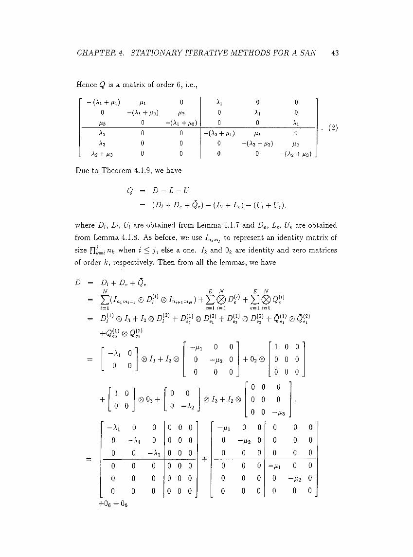
Hence Q is a. matrix of order 6, i.e.,
— (Ai + 0 - 1 0 00 —(Ai + 2) 0 0
Ai3 0 —(Ai + /is) 0 0 AiA2 0 0 " * ( - ^ 2 + Pi) /^1 0Ao 0 0 0 “"(A2 + A2 ) A2
Ao + /^ 3 0 0 0 0 —(A2 + / 3) .
• ( 2 )
Due to Theorem 4.1.9, we have
Q = D - L - U
— {Dt + De, + Qe) ~ (Ll + Z'e) ~ {I'l + f'e),
where Di, Li, Ui are obtained from Lemma 4.1.7 and Dg, Lg, Ug are obtained from Lemma 4.1.8. As before, we use to represent an identity matrix of size nl—i when i < j , else a one. R and Ot are identity and zero matricesof order A:, respectively. Then from all the lemmas, we have
(<)
D — Di Dg + Qe
= 0 a “ ’ 0 A , + E ® A '· + E ®¿=1 e=l ¿=1 e=l ¿ = 1
= 0 h + h & o f ' + £><;' 0 A f + A ! ’ 0 A ? + OS!' 0 OS!'
+0S !' 0 OS!’
—Ai 0
00
® /3 + /2 0 00
0 0
~H2 0
0 0
’ 1 0 0 ‘+ 0.2 0 0 0 0
_ 0 0 0 _
+’ 1 o' ' 0 o '
' 0 0 00 0.3 + 0 /3 + /2 0 0 0 0
0 0 _ 0 -A 2 __ 0 0 -/¿3 .
—Ai 0 0 0 0 0 ' -Ml 0 0 0 0 00 —Ai 0 0 0 0 0 -M2 0 0 0 00 0 -A i 0 0 0
+0 0 0 0 0 0
0 0 0 0 0 0 0 0 0 -Ml 0 00 0 0 0 0 0 0 0 0 0 -M2 0
0 0 0 0 0 0 0 0 0 0 0 0+ 0e + Og
CHAPTER 4. STATIONARY ITERATIVE METHODS FOR A SAN 44
+
0 0 0 0 0 0 0 0 0 0 0 00 0 0 0 0 0 0 0 0 0 0 00 0 0 0 0 0
+0 0 -^3 0 0 0
0 0 0 -Ao 0 0 0 0 0 0 0 00 0 0 0 —A2 0 0 0 0 0 0 00 0 0 0 0 — A2 0 0 0 0 0 -fi-i
-(A1 + Ai) 0 0 0 0 00 —(Ai + H2) 0 0 0 00 0 —(Ai -l· fi's) 0 0 00 0 0 -(A2 + Al) 0 00 0 0 0 -(A;2 + Ps) 00 0 0 0 0 — (A2+/i:3)
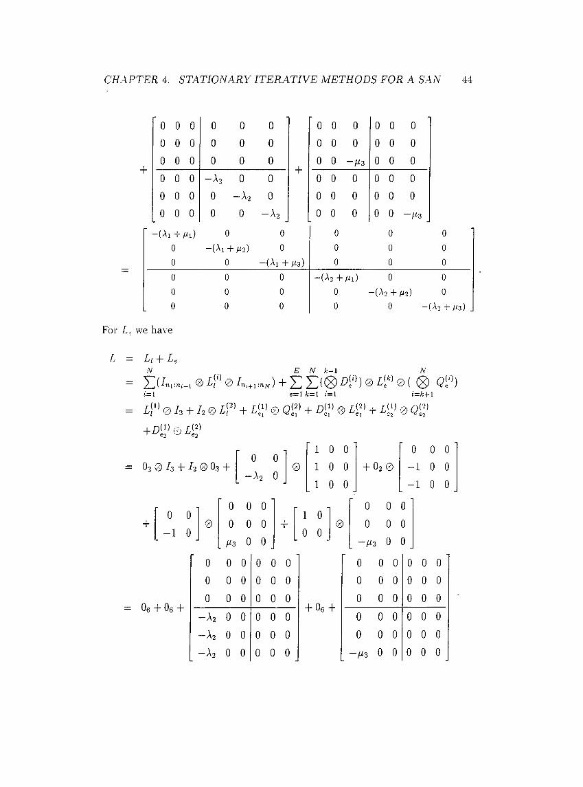
For L, we have
Zi = Li 4“ jZfN
‘ rii+i '-nN) + E E ( ® ^ f ’ ) 0 Z ‘ ’ 0( ® Q f )e = \ k = \ ¿=1 i= k -\ - ii=i
= £ i ‘ > 0 / , + / 2 0 ip> + £<;> 0 + £)<;' 0 £i;> + l h > 0 e g '
— 0 - 2 0 / 3 + - ^ 2 0 O3 +
’ 1 0 0 ‘ ' 0 0 0 '0 0
0 1 0 0 + O2 0 - 1 0 0-A2 0
_ 1 0 0 _ -1 0 0 _
+0 0
- 1 00
0 0 00 0 0
/2 3 0 0
+1 0
0 00
0 0 00 0 0
- ^ 3 0 0
— Oe + Oe +
0 0 0 0 0 0 ' 0 0 0 0 0 0
0 0 0 0 0 0 0 0 0 0 0 0
0 0 0 0 0 0+ Oe +
0 0 0 0 0 0
—A2 0 0 0 0 0 0 0 0 0 0 0
—A2 0 0 0 0 0 0 0 0 0 0 0
— A2 0 0 0 0 0 _ - / ¿ 3 0 0 0 0 0
CHAPTER 4. STATIONARY ITERATIVE METHODS FOR A SAN 45
+
0 0 0 0 0 0 0 0 0 0 0 0
0 0 0 0 0 0 0 0 0 0 0 0
-Ai.3 0 0 0 0 0 - M 3 0 0 0 0 0
0 0 0 0 0 0 — A2 0 0 0 0 0
0 0 0 0 0 0 — A2 0 0 0 0 0
0 0 0 0 0 0 — ( A 2 + Ms) 0 0 0 0 0
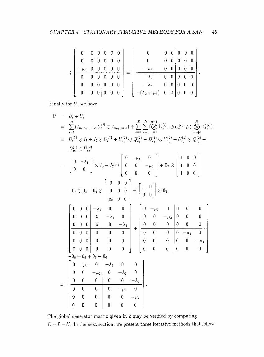
Finally for 1/, we have
U = Ui + U,N
= E ( i Ml :m,_i 7, f f V TJ UI vj 1 ,¿=i
(g) (?<■>)e= l ¿=1 ¿ = A:+1
= e /3 + /2 0 0 + D[\ 0 + u!;lj 0 +Dll 0 Fl')
00
-A i0
0 -Ml 0 1 0 03 + I 2 0 0 0 -M2 + O2 0 1 0 0
0 0 0 1 0 0
0 0 0-02 '<JO3 + O2 0 0 0 0
. / 3 0 0 _
0 0 0 -Ai 0 00 0 0 0 —Ai 00 0 0 0 0 -Ai0 0 0 0 0 00 0 0 0 0 00 0 0 0 0 0
+1 0
0 00 O3
+
0 -Ml 0 0 0 00 0 -M2 0 0 00 0 0 0 0 00 0 0 0 -Ml 00 0 0 0 0 -M20 0 0 0 0 0
+ 0e + Oe + Oe + 0$0 -Ml 0 —Ax 0 00 0 -M2 0 -Ax 00 0 0 0 0 —Ax0 0 0 0 -Ml 00 0 0 0 0 -M20 0 0 0 0 0
The global generator matrix given in 2 may be verified by computing D — L — U. In the next section, we present three iterative methods that follow
CHAPTER 4. STATIONARY ITERATIVE METHODS EOR A SAN 46
from the splitting in Theorem 4.1.9.
4.2 Iterative Methods Based on Splittings
Remember that the problem of finding the stationary vector of a Markov chain may be formulated as one of computing a nontrivial solution to a homogeneous system of linear algebraic ecfuations with a singular coefficient matrix under a normalization constraint. That is, the (1 x n) unknown vector tt in
■Q = 0. ||7r||i = 1 (3)
is sought. The methods based on splittings amount to using the power method with an iteration matrix that corresponds to the particular splitting until a predetermined stopping criterion is met. VVe should also remark thiit the efficient vector-(generalized) tensor product multiplication algorithm used by the methods of interest has a time complexity of order 0 (ni=i complexity result assumes that all matrices in a tensor product are dense. In reality, some of these matrices are identity and zero, some are diagonal, and the remaining sparse. .See, for instance, the matrices forming the descriptor in the example in Subsection 4.1.1.
In the following subsections, we introduce the stationary iterative methods of .Jacobi, Gauss-Seidel and SOR that we described in Chapter 2. In Section 4.3. we describe the block versions of the same methods.
4.2.1 Jacobi
In matrix notation, applying the .Jacobi method to a homogeneous linear sys
tem as in (3 ) is equivalent to applying the power method to the iteration matrix
(L 4- U)D~^] that is,
(A.-+i) ^ + U)D~\ À: = 0 ,1 , . . . ,
where Q is split as D — U). As it can be seen from the given formulation,each iteration may be implemented in two steps. First, postmultiply the most
CHAPTER 4. STATIONARY ITERATIVE METHODS EOR A SAN 47
recent approximation with (L + f/), which is a sum of tensor products, and obtain Then postmultiply with D~^. This last step can beimplemented by multiplying the reciprocal of each diagonal element in D with the corresponding element of to give
4.2.2 Gauss-Seidel
In matrix notation, applying GS to a homogeneous system as in (3) is equivalent to applying the power method to the iteration matrix U{D — L)~^. However, in order to employ the efficient vector-tensor product multiplication algorithm, we propose a slightly different implementation of the method. ,A. backward GS iteration corresponds to the splitting Q — [D — L) — U and may be written as
The right hand side of the iteration requires the use of vector-tensor product multiplication. Once the right hand side is computed as bC\ the next step involves solving the lower triangular system of equations Similarly one can define forward GS using the splitting Q = {D — U) — L. In order to employ the efficient vector-tensor product multiplication algorithm, we should examine the nonzero structure of the matrix [D — L).
is a diagonal matrix of order n = flili from which all the diagonal elements of [D — L) come. That is, none of the nonzero elements of L, a strictly lower -triangular matrix, appear along the diagonal of [D — L).
By considering Lemmas 4.1.7, 4.1.8 and relabeling Li as Te=o, we can rewrite L as
L· = + E E ( ® o f ’ ) 0 d ‘ ’ ® ( <8 ) c f ’ )i=lE
= Ee=0
N k-1
e= l k=l 1 = 1
N
i=k+l
E « 8 ) i> f ' ) 0 4 ‘ ’ 0 { ® < ?f)k=l 1=1 ¿=¿+1
= Ed''((g)<3<'>) + Ei>S''e=0 i= 2 e=0
E ( ® £ ' « ) 0 i<‘ >0 ( (g) O P )k= 2 i= 2 i=k+l
e=0
where all are strictly lower triangular matrices formed by summing similar tensor products. For Qq (i.e., Li), all matrices except Lq in the tensor products are identity matrices.
Similarly, using Lemmas 4.1.6, 4.1.7, 4.1.8 and relabeling QC as D[‘I e for e = 1, 2, . . . , FI, we get
D = f ; + + ¿ ( 8 ( 3 ; ' '¿=1 e= l ¿ = 1 e= l ¿=1N 2E N
= E i . . » - , 0 A “ ’ 0 + E <8 ) D[·’ ·i=l e= l1=1
Next we expose the block structure of {D — L) and build the lower triangular solution on this structure.
Each matrix is the sum of N tensor products. All tensor products in this summation introduce nonzero entries to that are in mutually exclusive locations. In other words, each nonzero element in comes from a different tensor product. To see this, partition into rii blocks each of order n|I:2 ' t· Its lower triangular blocks come from the term pH q 0 . . . t andits diagonal blocks come from the remaining terms (i.e., terms that have as the first factor). Observe that block { i , j ) * > j of can be expressed as e(,· Qe )·’ where is the (i, j ) th element of Similarly, block( j . j ) of can be expressed as [E [~ 2(® f=2 '2> © (<8 >;=r-+i >where is the jth. diagonal element of
Given the above (first level) partitioning of F, our algorithm for solving tt in the system Tr{D — P) = b stems from the following observation. The linear equations for the subvector of ~ corresponding to the jth diagonal block of [D — P), denoted Itj, can be expressed as
E N
CHAPTER 4. STATIONARY ITERATIVE METHODS FOR A SAN 48
7T, ~ S' 7T,:¿ = j+ l Le=0 k=2
('i)
or as
j j,j G 5 7 77-1, . . . , 2, 1.
Here Dj j is the jth diagonal block of (F> - F), bj and Cj are respectively the
yth subvectors of b and c, the new right hand side.
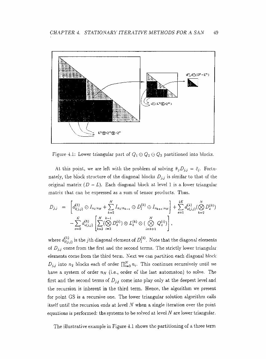
CHAPTER 4. STATIONARY ITERATIVE METHODS FOR A SAN 49
Q"
Figure 4.1; Lower triangular part of Q\ © Q 2 0 Q3 partitioned into blocks.
.A.t this point, we are left with the problem of solving I^jDjj — Cj. Fortunately, the block structure of the diagonal blocks Djj is similar to that of the original matrix (D — L). Each diagonal block at level 1 is a lower triangular matrix that can be expressed as a sum of tensor products. Thus.
411,> ®N
no'.71 TIN
-E 4Üe=0
j)
where is the j/'th diagonal element of D\ '. Note that the diagonal elements of Djj come from the first and the second terms. The strictly lower triangular- elements come from the third term. Next we can partition each diagonal block Djj into ri2 blocks each of order This continues recursively until wehave a system of order n v (i.e., order of the last automaton) to solve. The
first and the second terms of Djj come into play only at the deepest level and the recursion is inherent in the third term. Hence, the algorithm we present
for point GS is a recursive one. The lower triangular solution algorithm calls itself until the recursion ends at level N when a single iteration over the point equations is performed: the systems to be solved at level N are lower triangular.
k=2
(gi 0 S'<)k—2 1—2
2E N
e=l k = 2
The illustrative example in Figure 4.1 shows the partitioning of a three term
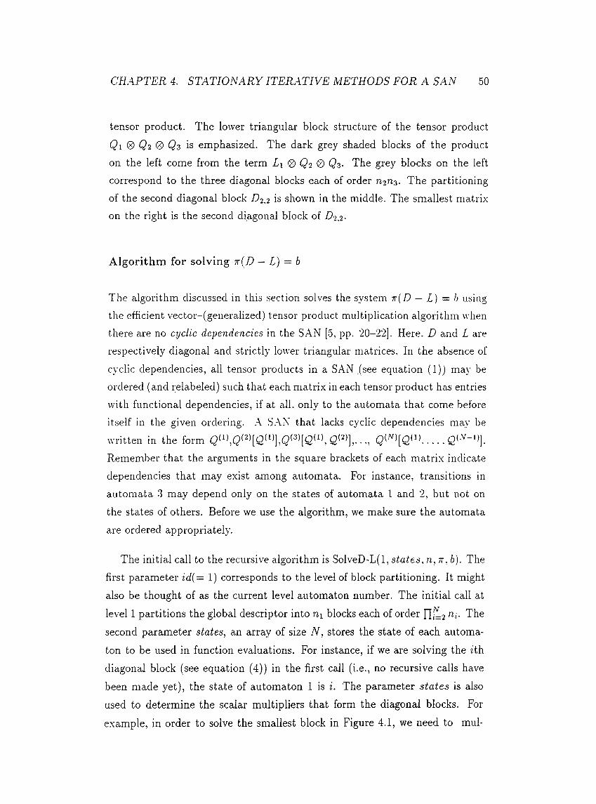
CHAPTER 4. STATIONARY ITERATIVE METHODS EOR A SAN 50
tensor product. The lower triangular block structure of the tensor product Qi ® Q 2 Qz is emphasized. The dark grey shaded blocks of the product on the left come from the term L\ @ Q 2 ® Qz- The grey blocks on the left correspond to the three diagonal blocks each of order n2nz· The partitioning of the second diagonal block D 2.2 is shown in the middle. The smallest matrix on the right is the second diagonal block of 1)2,2·
A lgorith m for solving - { D — L) = b
The algorithm discussed in this section solves the system 7r(Z) — L) = h using the efficient vector-(generalized) tensor product multiplication algorithm when there are no cyclic dependencies in the S.A.N [5, pp. 20- 22]. Here. D and L are respectively diagonal and strictly lower triangular matrices. In the absence of cyclic dependencies, all tensor products in a SAN (see ecjuation (1 )) may be ordered (and relabeled) such that each matrix in each tensor product has entries with functional dependencies, if at all. only to the automata that come before itself in the given ordering. .A. SAN that lacks cyclic dependencies may be
written in the form · ·; ........Remember that the arguments in the square brackets of each matrix indicate dependencies that may exist among automata. For instance, transitions in automata 3 may depend only on the states of automata 1 and 2, but not on the states of others. Before we use the algorithm, we make sure the automata are ordered appropriately.
The initial call to the recursive algorithm is SolveD-L(l, states, n, it, b). The first parameter id[= 1) corresponds to the level of block partitioning. It might also be thought of as the current level automaton number. The initial call at
level 1 partitions the global descriptor into rii blocks each of order n|I:2 ^1'· The second parameter states, an array of size N, stores the state of each automaton to be used in function evaluations. For instance, if we are solving the ¿th diagonal block (see equation (4)) in the first call (i.e., no recursive calls have been made yet), the state of automaton 1 is i. The parameter states is also used to determine the scalar multipliers that form the diagonal blocks. For
example, in order to solve the smallest block in Figure 4.1, we need to mul-
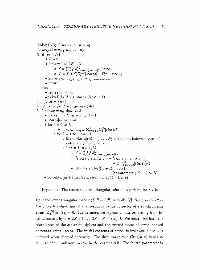
CHAPTER 4. STATIONARY ITERATIVE METHODS FOR A SAN 51
SolveD-L(z(/, states, f irs t , tt, b)1. nright = nid+iTiid+ 2 ■ --riM2. if {id = N)
• T = 0
• for e = 1 to 2E + iV
o T = T + diD^^^^^states] — [states])• Solve TTfirst —n,\/ + l:n rT = bf¡rst—ny+l:nM• return
else• states[id\ = Uid• SolveD-L(ic/ + 1, states, first, r, b)
3. - f i r s t = fir s t4. hfirst = f ir s t — [nidiiright) + 15. for trow = Uid dovvnto 2
• 7T f ir s t = TT firs t — nright + 1• states[id\ — irotu• for e = 0 to £■
O b = T^Trfirst:nrighti i=id+lQe‘ ['' ^ ^ ^ ]0 for A; = 1 to irow — 1
o Reset states[{id + 1 iV] to the first indexed states of automata {id + 1 ) to N
o for i = 1 to nright. j — Jl¥-^ rl T
i l j= l e[states[j]^states[j\)
^hfiTst-\-(k — \)nright-\-i—\ ^hJirst-{-[k — l)nTight-\-i—\
* Update siaies[('ic/+ 1) , iV]for automata {id + 1) to iV
• SolveD-L(fd + I, states, kf irst — nright + 1, tt, b)
Figure 4.2: The recursive lower triangular solution algorithm for SANs
tiply the lower triangular matrix with d2,2^ ,l· See also step 2 inthe SolveD-L algorithm; if e corresponds to the corrector of a synchronizing
event, [states] = 0. Furthermore, we represent matrices arising from local automata by e = 2E + 1 , . . . ,2E + N m step 2. We determine both the coordinates of the scalar multipliers and the current states of lower indexed automata using states. The initial contents of .states is irrelevant since it is updated when deemed necessary. The third parameter f ir s t {= n) is set to the size of the unknown vector in the current call. The fourth parameter is
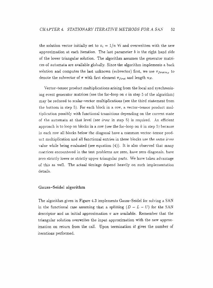
CHAPTER 4. STATIONARY ITERATIVE METHODS FOR A SAN 52
the solution vector initially set to tt,· = 1/n Vi and overwritten with the new approximation at each iteration. The last parameter b is the right hand side of the lower triangular solution. The algorithm assumes the generator matrices of automata are available globally. Since the algorithm implements a back solution and computes the last unknown (subvector) first, we use T’/irst-.n to denote the subvector of x with first element xfirst and length n¡\f.
Vector-tensor product multiplications arising from the local and synchronizing event generator matrices (see the for-loop on e in step 5 of the algorithm) may be reduced to scalar-vector multiplications (see the third statement from the bottom in step 5). For each block in a row, a vector-tensor product multiplication possibly with functional transitions depending on the current state of the automata at that level (see iroic in step 5) is recpiired. .An efficient approach is to loop on blocks in a row (see the for-loop on k in step 5) because in each row all blocks below the diagonal have a common vector-tensor product multiplication and all functional entries in these blocks use the same irotu value while being evaluated (see ecpiation (4)). It is also observed that many matrices encountered in the test problems are zero, have zero diagonals, have zero strictly lower or strictly upper triangular parts. We have taken advantage of this as well. The actual timings depend heavily on such implementation details.
Gauss—Seidel algorithm
The algorithm given in Figure 4.3 implements Gauss-Seidel for solving a SAN in the functional case assuming that a splitting {D — L — U) for the S.AN descriptor and an initial approximation x are available. Remember that the triangular solution overwrites the input approximation with the new approx
imation on return from the call. Upon termination it gives the number of
iterations performed.
CHAPTER 4. STATIONARY ITERATIVE METHODS FOR A SAN 53
• it = 0• Repeat until convergence
o it = it A 1o Compute b = irU o SolveD-L(l, n, 7T, 6)
Figure 4.3: The Gauss-Seidel algorithm using SolveD-L
4.2.3 Successive Overrelaxation
We now express the SOR method as := + (1 — w)AO
A O ■ . where>''SOR·is the (k + l)st approximation of GS, t sor approximation
of SOR. and lu is the relaxation parameter (i.e., a weighing factor) satisfying0 < w < 2.
4.3 Block Methods
We argued that one can perform a lower triangular back solution on the blocks of order at the final depth of recursion: see the third bullet in step 2 of the SolveD-L algorithm. Instead of doing this, one may choose to solve these blocks directly, i.e., by Gaussian elimination (GE). This approach, we call block GS, is likely to decrease the number of iterations since blocks at each iteration are solved exactly. When doing this, the right hand side b that goes into SolveD-L is computed in a slightly different manner. Now one must exclude the strictly upper triangular parts of the matrices corresponding to the last automaton from the multiplication. That is,
V /‘> 06 « =- ¿=1
Q A )e=l k = l i = l i = k + l
What has been excluded from the new right hand side must be included at level N in step 2 of the recursive back solution algorithm. The matrix that corresponds to automaton N at step 2 must include the whole matrices that
correspond to synchronizing events, their diagonal correctors and to local automata, not just the lower triangular parts. The matrices of order n.A/· formed in this way at the deepest level of recursion for each one of the diagonalblocks will be solved using GE. Even though the space requirement is larger, if the decrease in the iteration count is substantial the cost of solving the blocks directly is offset by a smaller overall solution time. Another possibility is to terminate recursion earlier and solve larger blocks. Also one can choose to generate and store larger blocks at the outset, then use these at each iteration (see the concept of grouping in [6, pp. 13-14]).
In the e.xperiments, we noticed an interesting feature of block methods.
R em ark 4.3.1 For a block coefficient matrix with lower (upper) triangular diagonal blocks in equation (S), backward (forward) block GS/SOR is equivalent to point GS/SOR.
The remark follows from inspecting the linear equations in systems with the described nonzero structure.
CHAPTER 4. STATIONARY ITERATIVE METHODS FOR A SAN 54
4.4 An Upper Bound on SolveD-L
In this section, we provide an upper bound on the number of multiplications performed in the SolveD-L algorithm for point GS (see subsection 4.2.2). Remember that multiplying the approximate subvector f j with block (j, i) j > i of the descriptor at the first level partitioning can be e.xpressed as e(] Qe^ )· index j in this expression changes, the product
Qe^ ) should be reevaluated for each value of j in case there are functional dependencies among automata. At worst, the value of the functional
rate remains constant for all blocks in the same row. We use the efficient vector-(generalized) tensor product multiplication algorithm that has a time
comple.xity of 0(111=1 tensor product with N matrices each oforder n,·. This complexity result assumes that all matrices that participate in the multiplication are dense.
CHAPTER 4. STATIONARY ITERATIVE METHODS FOR A SAN 55
In the following, T,· represents the number of multiplications performed in SolveD-L when the matrix to be solved is partitioned into n,· blocks each of
order riiLi+i nj.
T i = E (n¿ - 1 ) n . nj n j + i —j=¿+l i=¿+l
9 NI TT I 'TH------------- I I rij +
2 Nnr - Uin n,
j=i+l
Ty = E N
j-i+ln y {n y — 1)
for i <
, n ;v (n .v - l ) , ^H-------------------l· ENni ; + TlA¡.
The initial call to SolveD-L views the globed matrix as partitioned into ni blocks each of order ni=2 «· bounding Ti given by
Ti = EN N
(«1 - 1) n S ” < + o n ««· +9 A'n\ — ri\
JJ u, -1- UiTi.i—'2 i—2 i—2
The last term niT2 of T\ means in the next call we solve n\ diagonal blocks of order rii^2 recursively. The term that is inside the E parentheses arises from the multiplication of the current approximate subvector with tensor products corresponding to E synchronizing events. The first term (?2i — 1) 01^2 ^^^2
inside the parentheses is for the multiplication of the current approximate subvector with all blocks below the diagonal due to a synchronizing event. Remember that for each row of blocks all such multiplications are the same (hence we have ni — 1 of them), however each of the blocks below the diagonal gets
multiplied with a different scalar giving the second term {n\ — n i ) /2 n !^2
side the parentheses. In the first level of partitioning, (nl — n i)/2 is simply the number of blocks below the diagonal and n ¡^2 length of the subvector.The second term of Ti is for the number of scalar multiplications performed in computing the current approximate subvector-tensor product multiplication due to local automata. Note that the actual vector-tensor product multiplica
tions are accounted for as the first term inside the E parentheses.
In T(v, we have the number of scalar multiplications due to synchronizing events and due to local automata as the first and the second terms, respectively. The third term is for the number of multiplications performed in computing the diagonal corrector elements (i.e., each of the n/v diagonal elements in a
block gets multiplied with the diagonal elements of the previous N — I levels
CHAPTER 4. STATIONARY ITERATIVE METHODS FOR A SAN 56
and this happens for all E synchronizing events), and the last term is for the number of divisions made at level N to obtain the solution.
In order to find a closed form, vve write
Ti = E (ni - 1) +
+ ni E
i=2 i=2N N
n j — Til 9 n
1=2
2 N. '^1 “ TT ^
+ ;; 11
N
(n 2 - 1 ) H X ] H Hi
r -V N< E
¿■=3 ¿=3N
t=3+
¿=22 Nnf, — Tl2 ‘
1 3 rii + n-iTz¿=3
n - ' . - E ’-. + T H ·n;.¿=1 ¿=2
.V1 = 1
N
i= l
■ N N N
n XI + 2 n.¿ = 1 1=3 ¿=1
T—r+ — n « + «1^ 2 7:2 3
1 = 1N
<i=i
< E
< · ·
< E
■ NI
¿=2 .V N
Y^rii + Y^ mLz = 2 ¿=3
+ E■ N
Y ^ i,z=3
noUi U2
+ — + — ^ 9 9 Hi/2973
N
i=l
En "^('^^1 ”1" 2^ 2) +
ni TI2
9
-IJJ n, + ni'/iorsz = l
r :V NY r i i + ■■■ + Y r i i1 = 2 ¿=N
N-l+ JJ n,iTj\[.
i = l
N
J][ iz = l
N - l
t E >г7г;z=l
N N - l N
n + o XI nz=l z=i ¿=1
Noting thatN - l N
3 3 UiTy = - E N um 13 + :^EN 33 '2.· + 13 ”'' + 9 IIi= l ¿=1 i= l ¿=1 z = l
vve get the (loose) boundo N N 1 iV .V
Ti < + 9¿=1 ¿=1 i= l 1=1
Similarly one can find an upper bound on the number of multiplications
performed in computing the right hand side b as ( EN+1 ) HjXi n,· n l l i ^1· Here, E N is due to synchronizing events and 1 is due to local automata. Each tensor product arising from local automata has one upper triangular matrix; all others are identity. It is not surprising to find the total number of multiplications
performed in one iteration of the GS method on a SAN descriptor for the
algorithm given in this paper to be 0 { E N ni ni)·
Chapter 5
Numerical Results
5.1 The Problems and the Experiments
In order to make illuminating comparisons, we implemented power, Jacobi, GS. and SOR methods. We carried out experiments using both backward and forward versions of GS (and hence SOR) together with block versions of Jacobi. GS, and SOR methods. In block implementations, we terminate recursion at the deepest level and solve the blocks of order n/v using Gaussian elimination as discussed in Section 4.3. During the experiments we used a stopping criterion of between consecutive approximations. That is, we computed a residualvector as the difference between consecutive approximations, and used the 2- norm of this vector as the stopping criterion. We used a uniformly distributed probability vector as the initial approximation for all experiments. We ran all the experiments on SUN Sparcstation 4’s each with 32 megabytes (MB) of RAM. All the algorithms are implemented in C + + language and the new methods are incorporated into the software package PEPS [12]. Regardless of its size, each problem produced a smaller number of iterations in either the backward or the forward approach; we present results of the better approach.
We experimented with three problems. The first two, resource sharing and three queues, are explained in [5]. The third one, the model of a mass storage system, appears in [3]. For the mass storage example, we experimented with
ot
CHAPTER -5. NUMERICAL RESULTS 58
different orderings of the automata. Obviously, ordering of automata is likely to have an effect on the iteration count. The efficient vector-tensor product multiplication algorithm itself imposes an ordering on the automata. In order to use other orderings, a permutation vector may need to be introduced to the multiplication algorithm. We experimented with orderings that do not require permutation. We also tried orderings different from the original ordering by taking advantage of the position of identity matrices in tensor products. Such orderings follow from Lemma 5.5 and its companion remark in [5, p. 16].
Modeling with SANs is still in its infancy, and only recently have researchers started considering large and comple.x problems. Issues related to cyclic dependencies are currently under investigation. Lemma 5.8 and Theorem 5.2 in [5] show how one can handle cyclic dependencies in generalized tensor products. If the functional dependency graph is fully connected there is not much that can be done to improve the complexity of vector-generalized tensor product multiplication. On the other hand, if the cutset of the cycles in the dependency graph has a small number of automata, then a more efficient vector-generalized tensor product multiplication algorithm can be used. However, this multiplication will still take much longer than that of a vector-generalized tensor product lacking cycles. The smaller the cutset, the better the improvement. Moreover, at the end of Section 6 in [5], it is indicated that Theorem 5.2 needs to be used only when routing probabilities associated with synchronizing events (i.e., descriptors of slave automata due to synchronizing events) are functional and result in cycles within the functional dependency graph. The occurrence of this situation is suspected to be rare by the authors of [5]. We have not seen such a case. However, it is still not impossible to have generalized tensor products with dependency cycles. We should emphasize that no attempt has been made to avoid cyclic dependencies in the modeling phase of the mass storage problem. In [6], the last paragraph of subsection 4.3 discusses the results of some e.xperiments with artificially created cyclic dependencies. There it is
mentioned that cycles have a detrimental effect on solution time, as expected.
As for ordering the automata in the case of non-cyclic dependencies, we think it should not be very difficult. It is an implementation issue. However, we have purposefully concentrated on orderings that do not require the introduction of
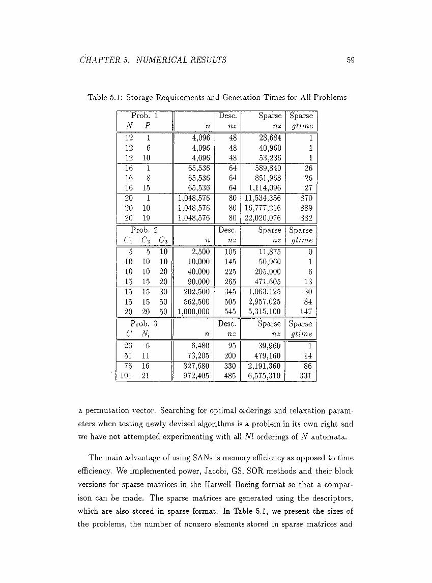
CHAPTER 0. NUMERICAL RESULTS 59
Table 5.1: Storage Requirements and Generation Times for All Problems
Prob. 1 Desc. Sparse SparseN P n nz nz gtime12 1 4,096 48 28,684 112 6 4,096 48 40,960 112 10 4,096 48 53,236 116 1 65,536 64 589,840 2616 8 65,536 64 851,968 2616 15 65,536 64 1,114,096 2720 1 1,048,576 80 11,534,.356 87020 10 1,048,576 80 16,777,216 88920 19 1,048,576 80 22,020,076 882
Prob. 2 Desc. Sparse Sparsec\ C‘2 C3 n nz nz gtime
5 5 10 2,500 105 11,875 010 10 10 10,000 145 50,960 110 10 20 40,000 225 205,000 615 15 20 90,000 265 471,605 1315 15 .30 202,500 345 1,063,125 3015 15 50 562,500 505 2,957,025 8420 20 50 1,000,000 545 5,315,100 147
Prob. 3 Desc. Sparse SparseC iV, n nz nz gtime26 6 6,480 95 39,960 151 11 73,205 200 479,160 1476 16 327,680 330 2,191,360 86
101 21 972,405 485 6,575,310 331
a permutation vector. Searching for optimal orderings and relaxation parameters when testing newly devised algorithms is a problem in its own right and we have not attempted experimenting with all N1 orderings of automata.
The main advantage of using SANs is memory efficiency as opposed to time efficiency. We implemented power, Jacobi, GS, SOR methods and their block
versions for sparse matrices in the Harwell-Boeing format so that a compar
ison can be made. The sparse matrices are generated using the descriptors, which are also stored in sparse format. In Table 5.1, we present the sizes of the problems, the number of nonzero elements stored in sparse matrices and
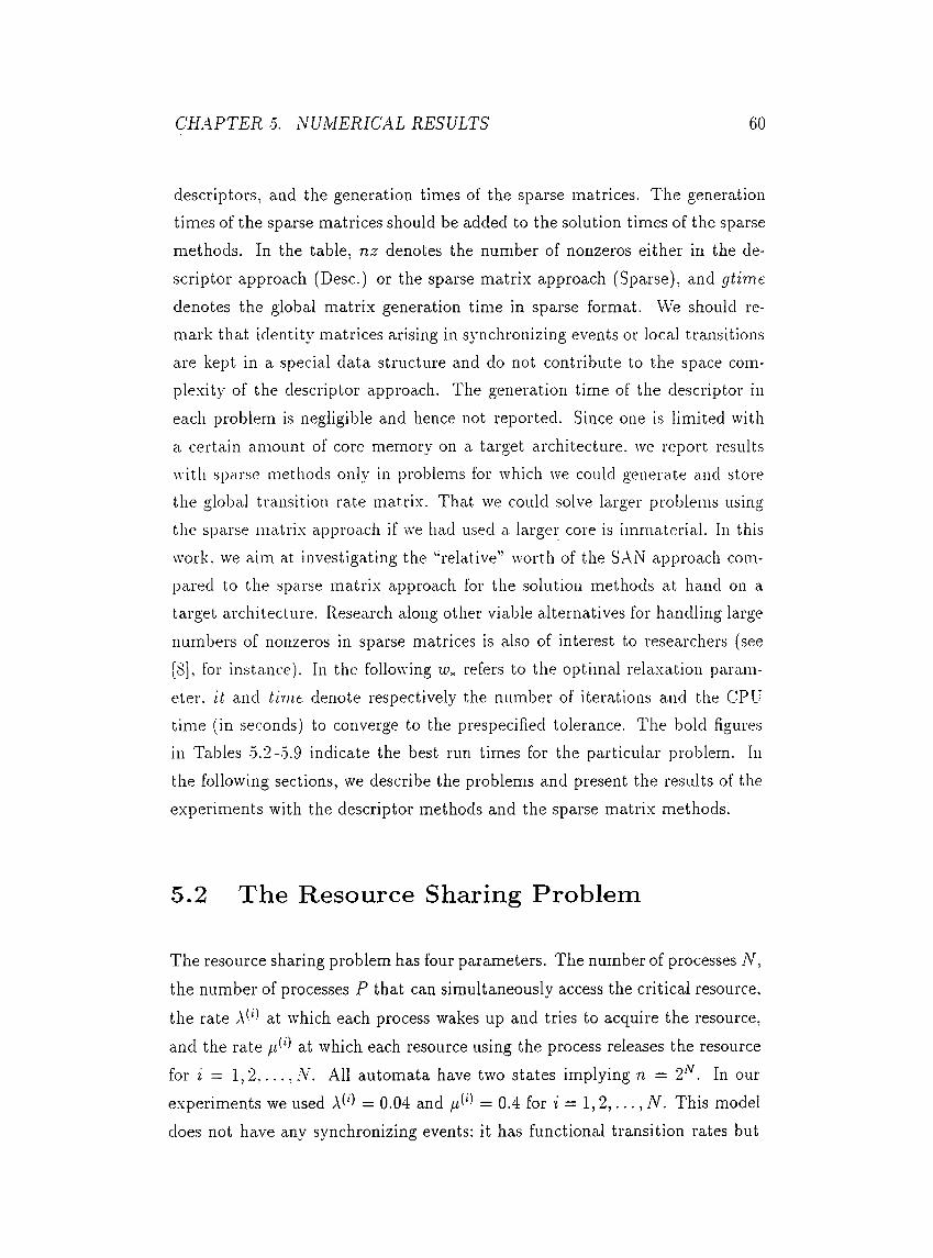
CHAPTER 0. NUMERICAL RESULTS 60
descriptors, and the generation times of the sparse matrices. The generation times of the sparse matrices should be added to the solution times of the sparse methods. In the table, nz denotes the number of nonzeros either in the descriptor approach (Desc.) or the sparse matrix approach (Sparse), and gtime denotes the global matrix generation time in sparse format. We should remark that identity matrices arising in synchronizing events or local transitions are kept in a special data structure and do not contribute to the space complexity of the descriptor approach. The generation time of the descriptor in each problem is negligible and hence not reported. Since one is limited with a certain amount of core memory on a target architecture, we report results with sparse methods only in problems for which we could generate and store the global transition rate matrix. That we could solve larger problems using the sparse matrix approach if we had used a larger core is immaterial. In this work, we aim at investigating the 'h'elative” worth of the SAN approach compared to the sparse matrix approach for the solution methods at hand on a target architecture. Research along other viable alternatives for handling large numbers of nonzeros in sparse matrices is also of interest to researchers (see [S], for instimce). In the following re« refers to the optimal reUixation parameter, it and time denote respectively the number of iterations and the CPU time (in seconds) to converge to the prespecihed tolerance. The bold figures in Tables 5.2-5.9 indicate the best run times for the particular problem. In the following sections, we describe the problems and present the results of the experiments with the descriptor methods and the sparse matrix methods.
5.2 The Resource Sharing Problem
The resource sharing problem has four parameters. The number of processes N, the number of processes P that can simultaneously access the critical resource,
the rate NP at which each process wakes up and tries to acquire the resource, and the rate at which each resource using the process releases the resource for i - 1 , 2 , . . . . N . All automata have two states implying n = 2‘^. In our experiments we used = 0.04 and = 0.4 for f = 1 ,2 , . . . , N. This model does not have any synchronizing events: it has functional transition rates but
CHAPTER 5. NUMERICAL RESULTS 61
Table 0.2: Results of Desc. Experiments with the Resource Sharing Problem
Prob. 1 Power GS SOR Block GS Block SORN P it tim e it t irrte it tim e it tim e it tim.e
12 1 142 83 2 2 1.0 2 2 2 2 1.0 2 212 6 222 131 26 23 1.3 18 16 26 22 1.3 18 1512 11 222 123 28 25 1.3 18 16 26 22 1.3 18 1516 1 188 2.299 2 39 1.0 2 40 2 38 1.0 2 3816 8 294 3.793 32 613 1.3 22 420 32 -592 1.3 22 40216 1-5 294 3.-562 34 650 1.4 22 420 32 589 1.3 22 40220 1 236 63.265 2 825 1.0 2 826 2 740 1.0 2 74020 10 362 94.157 38 15.0-39 1.5 26 9,777 38 13,764 1.4 24 8,73420 19 364 89.126 40 15.554 1.5 24 8,891 40 14,311 1.5 24 8.673
Table 0.·): Results of Sparse eriments with the Resource Sharing ProblemO
Prol) . 1 Power GS SOR B lock GS Block SOR.V P it t im e it t im e it t im e it t im e it t im e
12 1 142 4 2 0 1.0 2 0 . 2 0 1.0 2 012 6 222 9 26 1 1.3 18 1 26 2 1.3 18 112 11 222 12 28 2 1.3 18 1 26 2 1.3 18 216 1 188 118 2 2 1.0 2 2 2 3 1.0 2 316 8 294 255 32 30 1.3 22 22 32 52 1.3 22 3716 15 294 326 34 39 1.4 22 29 32 63 1.3 22 44
no cyclic dependencies. Since all matrices are identical for the given and fCK reordering the automata is futile. The resource sharing problem does not converge for .Jacobi and block .Jacobi methods. .As for backward block GS and
SOR methods, they are expected to give (slightly) smaller iteration counts than their point versions when P is closer to /V than to 0. This follows from Remark 4.1 and is particularly substantiated for the GS iteration. When P is small compared to .V. many of the upper diagonal elements of the 2 x 2 matrices evaluate to zero and there is no advantage of using block methods. On the other hand, when P is larger, many functional rates evaluate to nonzero values and the block methods start to make a diiference, however very little due to the extremely small block size. The results of the experiments are summarized in Table 5.2 and in Table 5.3. Observe that block SOR takes approximately 1/lOth of the time power method takes for the case N = 20, P = 19, in the descriptor approach. We were not able to solve the largest three instances of the this problem with a sparse solver.
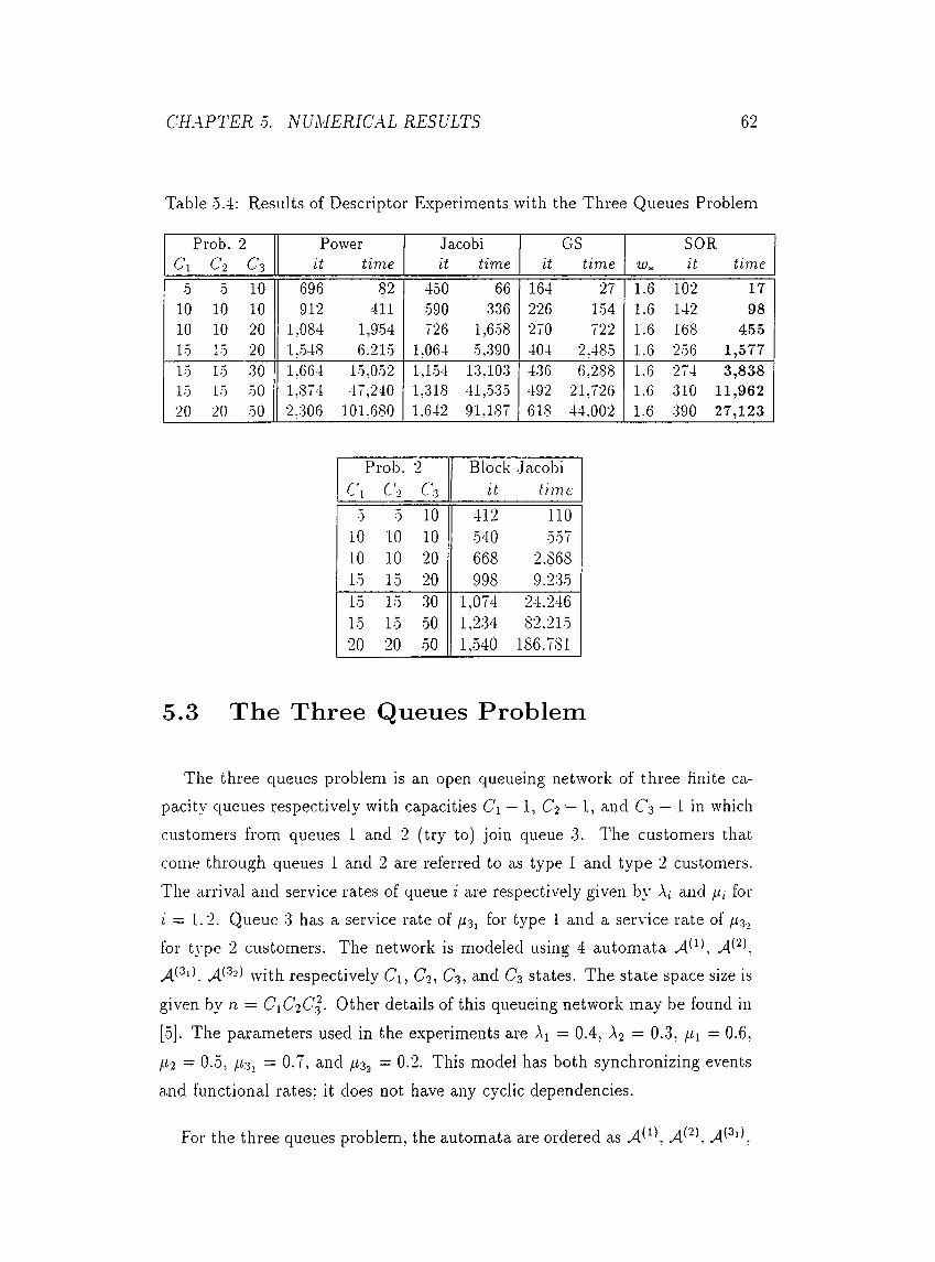
CHAPTER 0. NUMERICAL RESULTS 62
Table 5.4: Results of Descriptor Experiments with the Three Queues Problem
Prob. 2 Power Jacobi GS SORCl C2 C3 i t t im e it t im e it t i m e it t im e
5 5 10 696 82 450 66 164 ■21 1.6 102 1710 10 10 912 411 590 .336 226 1.54 1.6 142 9810 10 20 1,084 1,954 726 1,658 270 722 1.6 168 45515 15 20 1,548 6.215 1,064 5,.390 404 2,485 1.6 256 1,57715 15 30 1,664 15.052 1.154 13,103 436 6,288 1.6 274 3,83815 15 50 l ’874 47,240 1,318 41,.535 492 21,726 1.6 310 11,96220 20 50 2,306 101.680 1.642 91,187 618 44,002 1.6 390 27,123
Prob. 2 Block .JacobiCl C2 C3 it time
5 5 10 412 11010 10 10 540 55710 10 20 668 2.86815 15 20 998 9.23515 15 30 1,074 24.24615 15 50 1,234 82.21520 20 50 1,540 186.781
5.3 The Three Queues Problem
The three cpieues problem is an open cjueueing network of three finite Cci-
pacity queues respectively with capacities C\ — 1, CL — 1, and C3 — 1 in which customers from queues 1 and 2 (try to) join cpieue 3. The customers that come through queues 1 and 2 are referred to as type 1 and type 2 customers. The arrival and service rates of queue i are respectively given by A,· and /q for i = 1.2. Queue 3 has a service rate of for type 1 cind a service rate of /¿3. for type 2 customers. The network is modeled using 4 automata A 'K^(3i) ^ (32) with respectively Ci, C2, C3, and C3 states. The state space size is
given by n = CiC-iCl- Other details of this queueing network may be found in [5]. The parameters used in the experiments are Ai = 0.4, A2 — 0.3, ¡jL]_ - 0.6, l-i2 = 0.5, /[¿3, = 0.7, and /¿3, = 0.2. This model has both synchronizing events and functional rates; it does not have any cyclic dependencies.
For the three queues problem, the automata are ordered as
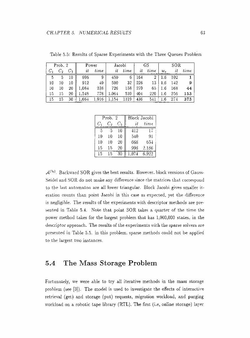
CHAPTER 5. NUMERICAL RESULTS 63
Table 0.5 : Results of Sparse Experiments with the Three Queues Problem
CxProb.
C-22С.з
Power it time
Jacobi it time it
GStime
SORit time
5 5 10 696 9 450 6 164 2 1.6 102 110 10 10 912 49 590 32 226 13 1.6 142 910 10 20 1,084 238 726 1-58 270 6-5 1.6 168 4415 15 20 1,-548 778 1.064 -539 404 220 1.6 256 15315 15 30 1,664 1,916 1,1-54 1319 436 -541 1.6 274 373
Prob.c \ C l
2
СзBlock
it.Jacobi
time5 5 10 412 17
10 10 10 540 9110 10 20 668 65415 15 20 998 2.18615 15 30 1,074 6.922
. Backward SOR gives the best results. However, block versions of Gauss- Seidel and SOR do not make any difference since the matrices that correspond to the last automaton are all lower triangular. Block .Jacobi gives smaller iteration counts than point .Jacobi in this case as expected, yet the difference is negligible. The results of the experiments with descriptor methods are presented in Table 5.4. Note that point SOR takes a ciuarter of the time the power method takes for the largest problem that has 1,000,000 states, in the descriptor approach. The results of the experiments with the sparse solvers are presented in Table 5.5. in this problem, sparse methods could not be applied to the largest two instances.
5.4 The Mass Storage Problem
Fortunately, we were able to try all iterative methods in the mass storage problem (see [3]). The model is used to investigate the effects of interactive retrieval (get) and storage (put) requests, migration workload, and purging workload on a robotic tape library (RTL). The first (i.e, online storage) layer
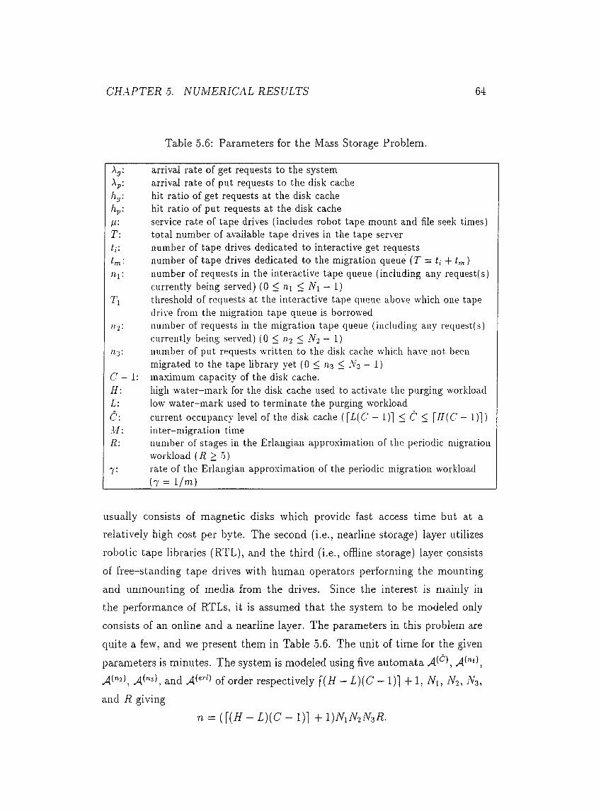
CHAPTER 5. NUMERICAL RESULTS 64
Table 5.6: Parameters for the Mass Storage Problem.
hp. ¡.t:T:t't’ Cl ·iii:
n·)·
n'y.
C - 1: // :L:C:M:R:
7·
arrival rate of get requests to the system arrival rate of put requests to the disk cache hit ratio of get requests at the disk cache hit ratio of put requests at the disk cacheservice rate of tape drives (includes robot tape mount and file seek times)total number of available tape drives in the tape servernumber of tape drives dedicated to interactive get requestsnumber of tape drives dedicated to the migration queue (T = ti + tm)number of requests in the interactive tape queue (including any request(s)currently being served) (0 < rii < jVi - 1)threshold of requests at the interactive tape queue above which one tape drive from the migration tape queue is borrowednumber of requests in the migration tape queue (including any request(s) currently being served) (0 < n-2 < N2 - 1 )number of put requests written to the disk cache which have not been migrated to the tape library yet (0 < ^3 < .V3 — 1) maximum capacity of the disk cache.high water-mark for the disk cache used to activate the purging workload low water-mark used to terminate the purging workload current occupancy level of the disk cache (\L{C - 1)] < C < \H(C - 1)]) inter-migration timenumber of stages in the Erlangian approximation of the periodic migration workload (i2 > 0 )rate of the Erlangian approximation of the periodic migration workload(7 = l/m)
usually consists of magnetic disks which provide fast access time but at a relatively high cost per byte. The second (i.e., nearline storage) layer utilizes robotic tape libraries (RTL), and the third (i.e., offline storage) layer consists of free-standing tape drives with human operators performing the mounting and unmounting of media from the drives. Since the interest is mainly in the performance of RTLs, it is assumed that the system to be modeled only consists of an online and a nearline layer. The parameters in this problem are
ciuite a few, and we present them in Table 5.6. The unit of time for the given parameters is minutes. The system is modeled using five automata
^ ("3) and of order respectively — L)(C — 1)] + 1, Ni, No·, A3,and R giving
n = L)(C - 1)1 + l)/ViyV2iVsR.
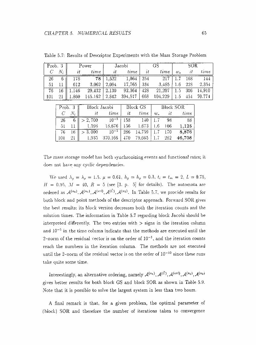
CHAPTER 5. NUMERICAL RESULTS 65
Table 5.7: Re.sults of Descriptor Experiments with the Mass Storage Problem
Prob.. 3 Power Jacobi GS SORC Ah it time it time it time it time
26 6 178 78 1,522 1,064 254 217 1.7 168 14451 11 612 3,062 2,084 17,765 334 3,485 1.6 228 2.35476 16 1.146 29,432 2,130 92,364 428 21,207 1.5 306 14,910
101 21 1.860 145,162 2,842 394,517 668 104.229 1.0 454 70.774
Prob. 3 Block Jacobi Block GS Block SORC N\ it time it time гСх it time26 6 > 2,700 10“ ’ 158 140 1.7 98 8851 11 1.-598 18.676 156 1.673 1.6 106 1,12576 16 > 3.000 10“ ’ 286 14.759 1.7 170 8,876
101 21 1,935 370.166 470 79,665 1.7 282 46,708
The mass storage model has both synchronizing events and functional rates; it does not have any cyclic dependencies.
We used = \p = 1.5. f.i = 0.61. = hp = 0.3, ti — t,n = 2. L = 0.75,/■/ = 0.05. M = 40, R = 0 (see [3. p. 5] for details). The automata are ordered as In Table 5.7, we provide results forboth block and point methods of the descriptor approach. Forward SOR gives the best results: its block version decreases both the iteration counts and the solution times. The information in Table 5.7 regarding block .Jacobi should be interpreted differently. The two entries with > signs in the iteration column and 10“ ’ in the time column indicate that the methods are executed until the 2-norm of the residual vector is on the order of 10“ ’ , and the iteration counts reach the numbers in the iteration column. The methods are not executed until the 2-norm of the residual vector is on the order of 10“ ° since these runs take cpiite some time.
Interestingly, an alternative ordering, namely \ gives better results for both block GS and block SOR as shown in Table 5.9. Note that it is possible to solve the largest system in less than two hours.
A final remark is that, for a given problem, the optimal parameter of
(block) SOR and therefore the number of iterations taken to convergence
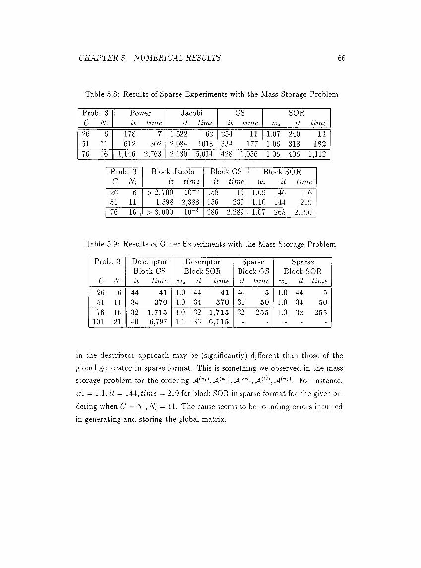
CHAPTER 5. NUMERICAL RESULTS 66
Table 5.8: Results of Sparse Experiments with the Mass Storage Problem
Prob. 3 Power .Jacobi GS SORC Ni it time it time it time lU it time26 6 178 7 1.Ô22 62 254 11 1.07 240 1151 11 612 302 2,084 1018 334 177 1.06 318 18276 16 1,146 2,763 2.130 5.014 428 1,056 1.06 406 1,112
Prob. 3 Block Jacobi Block GS Block SORC Ni it time it time it time
26 6 > 2,700 10-’ 158 16 1.09 146 1651 11 1,598 2.388 156 230 1.10 144 21976 16 > 3.000 10-’ 286 2.289 1.07 268 2.196
Table 5.9: Results of Other Experiments with the Mass Storage Problem
Prob.
C
. 3
■
Descriptor Block GSit time
Descriptor Block SOR
u;« it time
Sparse Block GS it time
Sparse Block SOR
7.0, it time26 6 44 41 1.0 44 41 44 5 1.0 44 551 11 34 370 1.0 34 370 34 50 1.0 34 5076 16 32 1,715 1.0 32 1,715 32 255 1.0 32 255
101 21 40 6,797 1.1 36 6,115 - - - -
in the descriptor approach may be (significantly) different than those of the global generator in sparse format. This is something we observed in the mass storage problem for the ordering For instance,uv - i .l , it - 144, time = 219 for block SOR in sparse format for the given or
dering when C = 51, iVi = 11. The cause seems to be rounding errors incurred in generating and storing the global matrix.
Chapter 6
Conclusion
In this work, we presented iterative methods based on splitting a SAN descriptor. Block versions of the same methods follow directly from considering blocks of order n,v, the order of the last automaton, in the given ordering. Larger blocks may be considered by grouping several automata at the end of the given ordering and terminating recursive calls of the lower triangular back solve algorithm when the first automata in the group is encountered.
By deriving cin upper bound on the Gauss-Seidel and SOR algorithms for the number of multiplications that is in the same order with the vector-descriptor multiplication, we show that the stationary methods are as efficient as non- stationary methods that do only vector-descriptor multiplications. Hence, we show that the solution times of a specific problem with different approaches depend only on the behavior of the algorithm for the given problem.
An important and frec[uently overlooked drawback of Markov chain solvers (including SAN solvers) that attempt at computing each and every stationary
probability is the memory consumed by double precision temporary storage allocated to the current approximation, possibly the preceding one, and other work arrays. A vector of one million elements requires 8 MB of memory. .Although not as large as the memory taken up by double precision nonzeros in the sparse matrix approach, these vectors may end up taking substantial space
in iterative methods.
CHAPTER 6. CONCLUSION 68
On a desktop workstation with 32 MB of RAM, one can compute the stationary distribution of a SAN descriptor with one million states in core on the order of hours using block SOR. On the other hand, the largest system that can be solved by the sparse matrix approach may be limited to less than one tenth of that could be solved using SANs if the generator is reasonably dense (as in the resource sharing problem; it takes roughly 176 MB to store the generator matrix in sparse format for the most difficult case). We believe the S.AN modeling methodology has its merits and drawbacks. One may easily observe that sparse methods must be used whenever possible. The .S.A.N formalism is likely to gain popularity as a viable modeling and analysis tool as faster solvers become available.
Appendix A
Incorporating a New Model To Peps
A .l Preliminaries
This section expiains how to incorporate a performance mociei. cieveioped as a SAN to the software package Peps [12]. It is assumeci that the mociei to incorporate must be avaiiabie; that is, iocai matrices anci synchronizing event matrices with their diagonai correctors must be avaiiabie. A mathematicai formuiation of functional rates should also be available, i.e.. one must know
how to evaluate the function given the state of the automata. In the remaining, we use ’Peps', to mean the latest revision of the package as it is implemented at Bilkent University. We use ‘original Peps’ to mean the version that is supplied to Bilkent University as in [12]. There are two steps to complete the task of adding a new model. First, one should generate a text file describing the model; second, the necessary code for evaluating the functional rates should be incorporated to the package. The two sections that follow explain these two
steps. The final section presents the text file for an example model.
69
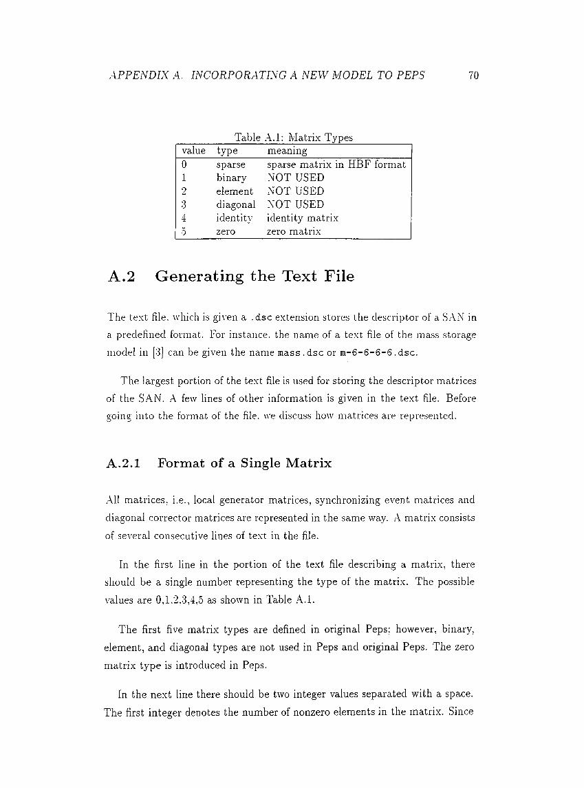
APPENDIX A. INCORPORATING A NEW MODEL TO PEPS 70
Table A .l: Matrix Typesvalue type meaning0 sparse sparse matrix in HBF format1 binary NOT USED2 element NOT USED3 diagonal NOT USED4 identity identity matrix0 zero zero matrix
A .2 Generating the Text File
The text file, which is given a .dsc extension stores the descriptor of a .SAN in a predefined format. For instance, the name of a text file of the mass storage model in [3] can be given the name mass .dsc or m -6 -6 -6 -6 .dsc.
The largest portion of the text file is used for storing the descriptor matrices of the S.AN. A few lines of other information is given in the text file. Before going into the format of the file, we discuss how matrices are represented.
A .2.1 Format of a Single Matrix
All matrices, i.e., local generator matrices, synchronizing event matrices and diagonal corrector matrices are represented in the same way. .A matrix consists of several consecutive lines of text in the file.
In the first line in the portion of the text file describing a matrix, there should be a single number representing the type of the matrix. The possible
values are 0,1.2,3,4.5 as shown in Table .A.l.
The first five matrix types are defined in original Peps; however, binary, element, and diagonal types are not used in Peps and original Peps. The zero
matrix type is introduced in Peps.
In the next line there should be two integer values separated with a space. The first integer denotes the number of nonzero elements in the matrix. Since
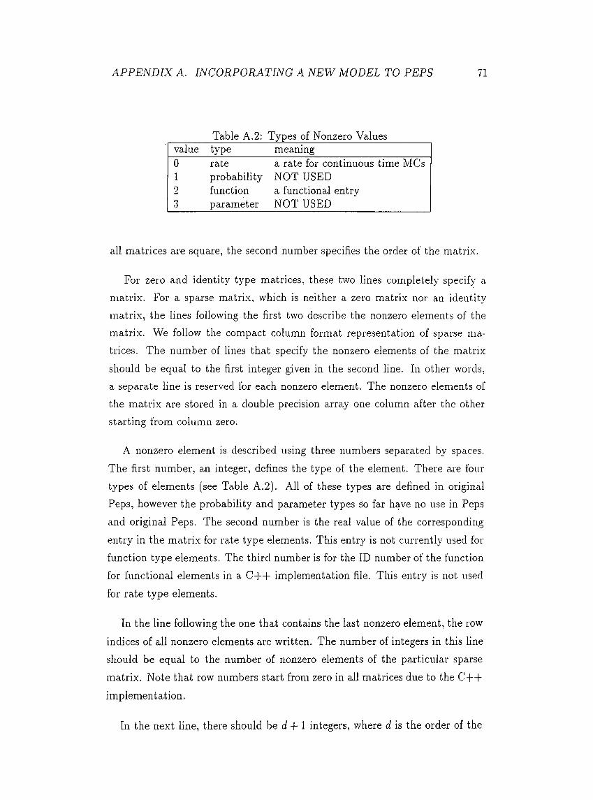
APPENDIX A. INCORPORATING A NEW MODEL TO PEPS 71
Table A.2: Types of Nonzero Valuesvalue type meaning0 rate a rate for continuous time MCs1 probability NOT USED2 function a functional entry.3 parameter NOT USED
all matrices are square, the second number specifies the order of the matrix.
For zero and identity type matrices, these two lines completely specify a matrix. For a sparse matrix, which is neither a zero matrix nor an identity matrix, the lines following the first two describe the nonzero elements of the matrix. We follow the compact column format representation of sparse matrices. The number of lines that specify the nonzero elements of the matrix should be equal to the first integer given in the second line. In other words, a separate line is reserved for each nonzero element. The nonzero elements of the matrix are stored in a double precision array one column after the other starting from column zero.
A nonzero element is described using three numbers separated by spaces. The first number, an integer, defines the type of the element. There are four types of elements (see Table A.2). All of these types are defined in original Peps, however the probability and parameter types so far have no use in Peps and original Peps. The second number is the real value of the corresponding entry in the matrix for rate type elements. This entry is not currently used for function type elements. The third number is for the ID number of the function for functional elements in a C + + implementation file. This entry is not used for rate type elements.
In the line following the one that contains the last nonzero element, the row indices of all nonzero elements are written. The number of integers in this line should be equal to the number of nonzero elements of the particular sparse matrix. Note that row numbers start from zero in all matrices due to the C + + implementation.
In the next line, there should be d + 1 integers, where d is the order of the
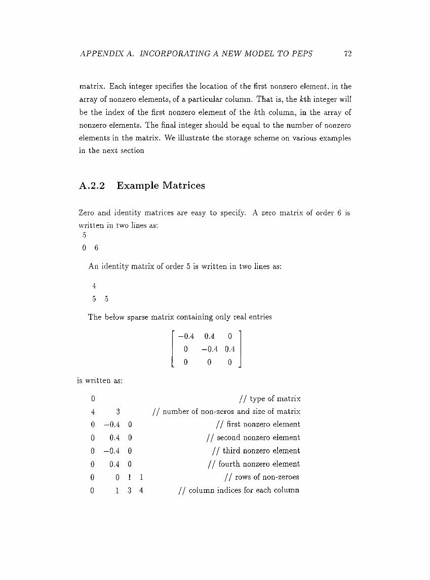
APPENDIX A. INCORPORATING A NEW MODEL TO PEPS 72
matrix. Each integer specifies the location of the first nonzero element, in the array of nonzero elements, of a particular column. That is, the kth integer will be the index of the first nonzero element of the A:th column, in the array of nonzero elements. The final integer should be equal to the number of nonzero elements in the matrix. We illustrate the storage scheme on various e.xamples in the next section
A .2.2 Example Matrices
Zero and identity matrices are easy to specify. A zero matrix of order 6 iswritten in two lines as:
0
0 6
An identity matrix of order 5 is written in two lines as:
45 5
The below sparse matrix containing only real entries
-0 .4 0.4 00 -0 .4 0.40 0 0
is written as:
0 / / type of matrix4 3 / / number of non-zeros and size of matrix
0 -0 .4 0 / / first nonzero element
0 0.4 0 / / second nonzero element
0 -0 .4 0 / / third nonzero element
0 0.4 0 / / fourth nonzero element
0 0 1 1 / / rows of non-zeroes
0 1 3 4 / / column indices for each column
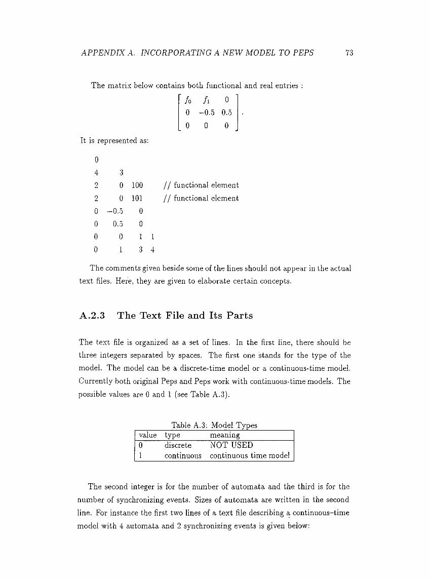
APPENDIX A. INCORPORATING A NEW MODEL TO PEPS 73
The matrix below contains both functional and real entries
fo / l 00 -0 .5 0.50 0 0
It is represented as:
04 32 0 100 / / functional element2 0 101 / / functional element0 -0 .5 00 0.5 00 0 1 10 1 3 4
The comments given beside some of the lines should not appear in the actual text files. Here, they are given to elaborate certain concepts.
A .2.3 The Text File and Its Parts
The text file is organized as a set of lines. In the first line, there should be three integers separated by spaces. The first one stands for the type of the model. The model can be a discrete-time model or a continuous-time model. Currently both original Peps and Peps work with continuous-time models. The possible values are 0 and 1 (see Table A.3).
Table A.3: Model Typesvalue type meaning0 discrete NOT USED1 continuous continuous time model
The second integer is for the number of automata and the third is for the number of synchronizing events. Sizes of automata are written in the second line. For instance the first two lines of a text file describing a continuous-time model with 4 automata and 2 synchronizing events is given below:
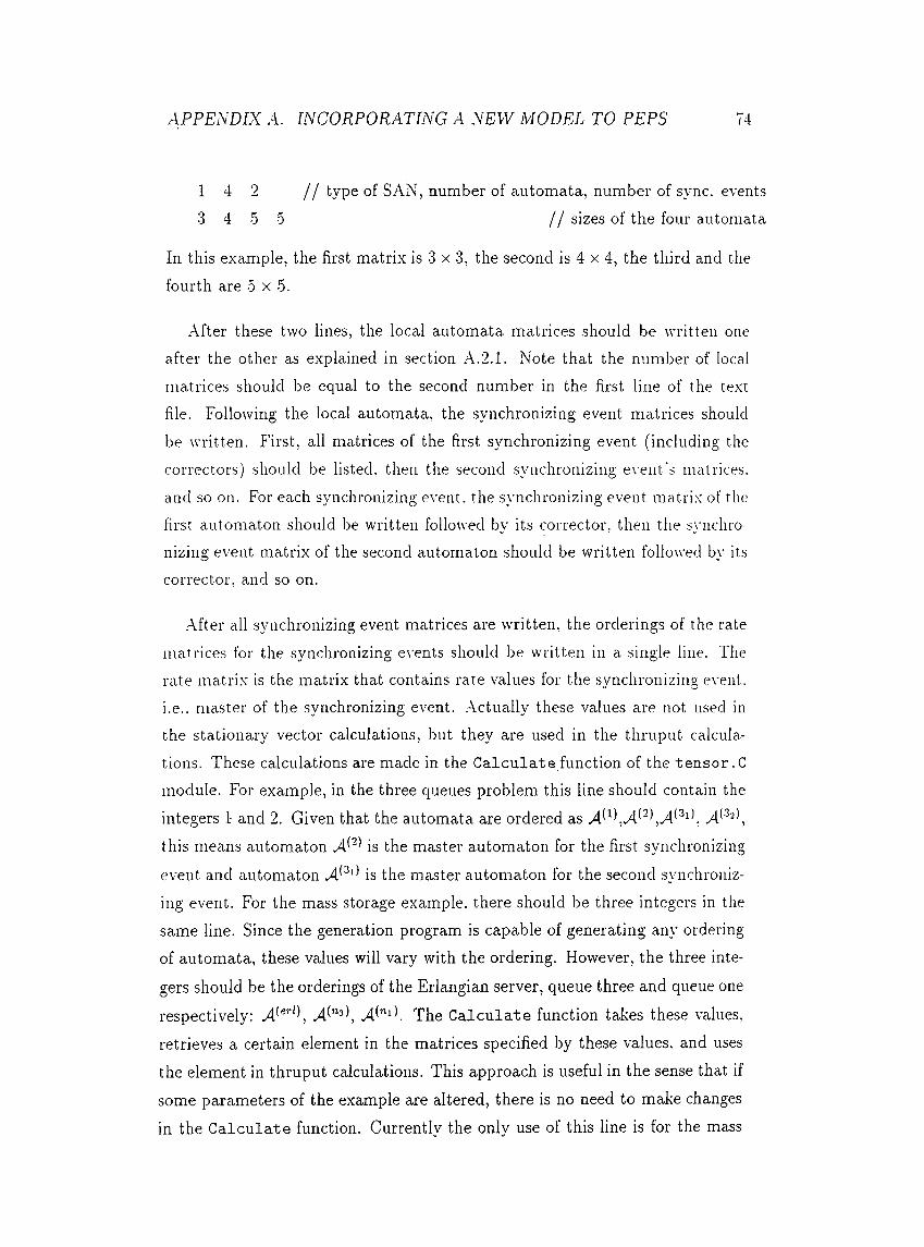
APPENDIX A. INCORPORATING A NEW MODEL TO PEPS 74
1 4 2 / / type of SAN, number of automata, number of sync, events3 4 5 5 / / sizes of the four automata
In this example, the first matrix is 3 x 3, the second is 4 x 4, the third and the fourth are 5 x 5.
After these two lines, the local automata matrices should be written one after the other as explained in section A.2.1. Note that the number of local matrices should be ecpial to the second number in the first line of the text file. Following the local automata, the synchronizing event matrices should be written. First, all matrices of the first synchronizing event (including the correctors) should be listed, then the second synchronizing event's matrices, and so on. For each synchronizing event, the synchronizing event matrix of the first automaton should be written followed by its corrector, then the synchronizing event matrix of the second automaton should be written followed by its corrector, and so on.
After all synchronizing event matrices are written, the orderings of the rate matrices for the synchronizing e\'ents should be written in a single line. The rate matrix is the matrix that contains rate values for the synchronizing event, i.e.. master of the synchronizing event. Actually these values are not used in the stationary vector calculations, but they are used in the thruput calculations. These calculations are made in the C alcu late function of the tensor. C module. For example, in the three C[ueues problem this line should contain the integers 1· and 2. Given that the automata are ordered asthis means automaton is the master automaton for the first synchronizingevent and automaton is the master automaton for the second synchronizing event. For the mass storage example, there should be three integers in the same line. Since the generation program is capable of generating any ordering of automata, these values will vary with the ordering. However, the three inte
gers should be the orderings of the Erlangian server, queue three and queue one respectively: The C alcu late function takes these values,retrieves a certain element in the matrices specified by these values, and uses the element in thruput calculations. This approach is useful in the sense that il some parameters of the example are altered, there is no need to make changes in the C alcu late function. Currentlv the onlv use of this line is lor the mass
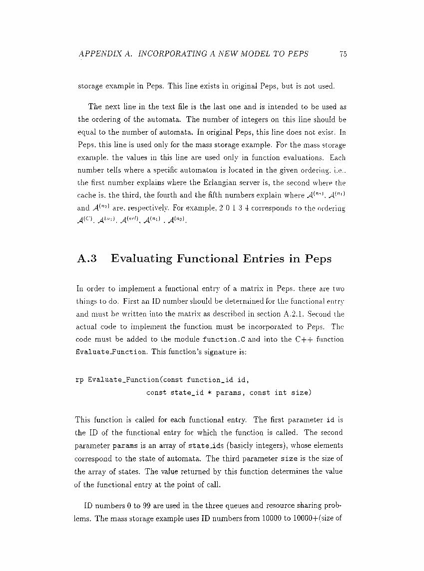
APPENDIX A. INCORPORATING A NEW MODEL TO PEPS /0
storage example in Peps. This line exists in original Peps, but is not used.
The next line in the text file is the last one and is intended to be used as the ordering of the automata. The number of integers on this line should be equal to the number of automata. In original Peps, this line does not e.xist. In Peps, this line is used only for the mass storage example. For the mass storage example, the values in this line are used only in function evaluations. Each number tells where a specific automaton is located in the given ordering, i.e.. the first number explains where the Erlangian server is, the second where the cache is. the third, the fourth and the fifth numbers explain where >1*"**. and >lb‘2) respectively. For example, 2 0 1 3 4 corresponds to the ordering
,4 0 m) _
A.3 Evaluating Functional Entries in Peps
In order to implement a functional entry of a matrix in Peps, there are two things to do. First an ID number should be determined for the functional entry and must be written into the matrix as described in section .A..2.1. Second the actual code to implement the function must be incorporated to Peps. The code must be added to the module fu n ction .C and into the C + + function Evaluate_Function. This function’s signature is:
rp Evaluât e_Funct ion (const fu n ction _ id id ,const sta te_ id * params, const in t s iz e )
This function is called for each functional entry. The first parameter id is the ID of the functional entry for which the function is called. The second parameter paraias is an array of state_ids (basicly integers), whose elements
correspond to the state of automata. The third parameter s iz e is the size of the array of states. The value returned by this function determines the value of the functional entry at the point of call.
ID numbers 0 to 99 are used in the three queues and resource sharing problems. The mass storage example uses ID numbers from 10000 to 10000+(size of
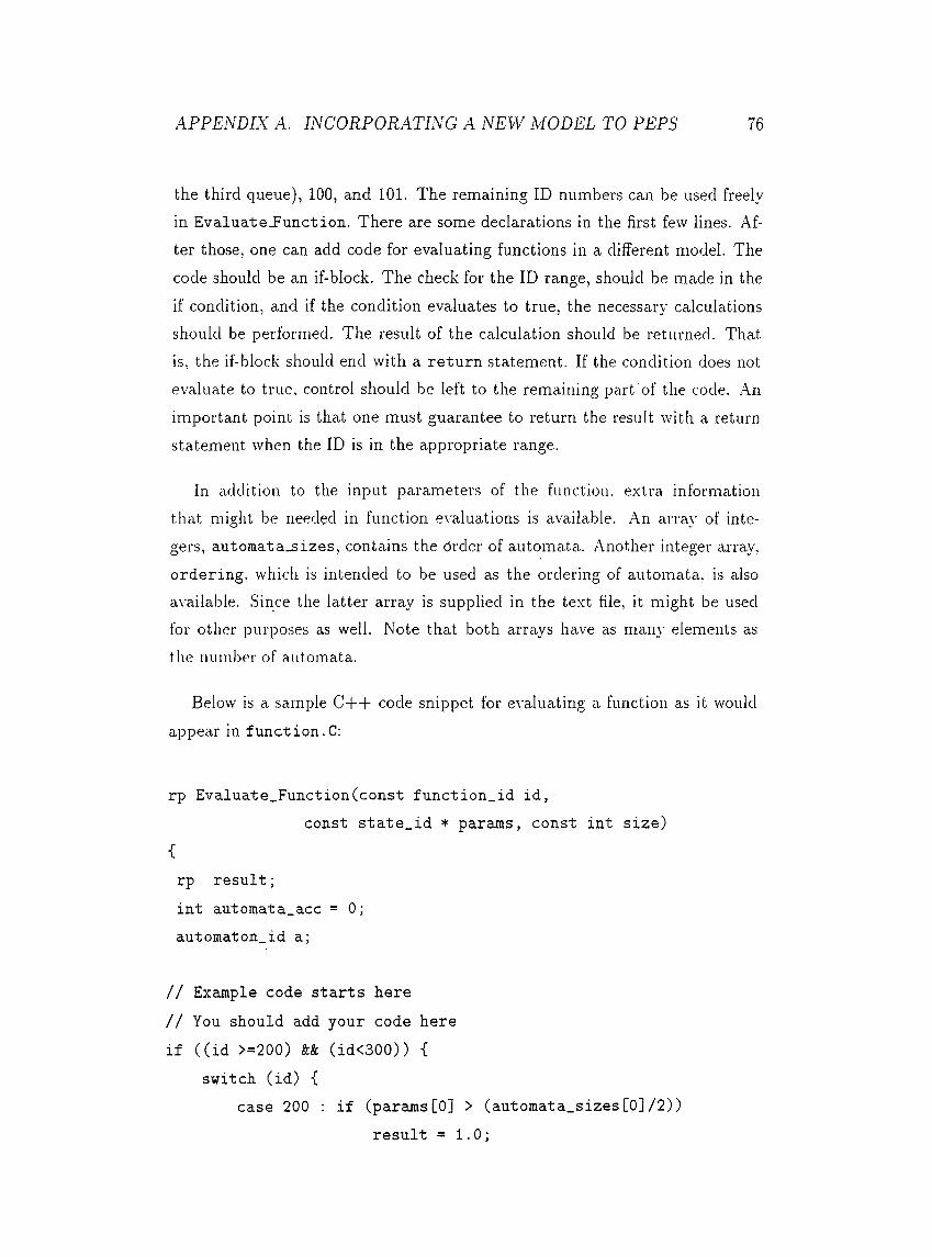
APPENDIX A. INCORPORATING A NEW MODEL TO PEPS 76
the third queue), 100, and 101. The remaining ID numbers can be used freely in Evaluâte_Function. There are some declarations in the first few lines. After those, one can add code for evaluating functions in a different model. The code should be an if-block. The check for the ID range, should be made in the if condition, and if the condition evaluates to true, the necessary calculations should be performed. The result of the calculation should be returned. That is, the if-block should end with a return statement. If the condition does not evaluate to true, control should be left to the remaining part of the code. An important point is that one must guarantee to return the result with a return statement when the ID is in the appropriate range.
In addition to the input parameters of the function, e.xtra information that might be needed in function evaluations is available. An array of integers, automata_sizes, contains the Order of automata. Another integer array, ordering, which is intended to be used as the ordering of automata, is also available. Since the latter array is supplied in the te.xt file, it might be used for other purposes as well. Note that both arrays have as many elements as the number of automata.
Below is a sample C-b+ code snippet for evaluating a function as it would appear in function .C ;
rp Evaluate_Function(const function_id id,const state_id * params, const int size)
{rp result ;int automata_acc = 0;automaton_id a;
// Example code starts here // You should add your code here if ((id >=200) && (idOOO)) {
switch (id) {case 200 : if (params[0] > (automata_sizes[0]/2))
result = 1.0;
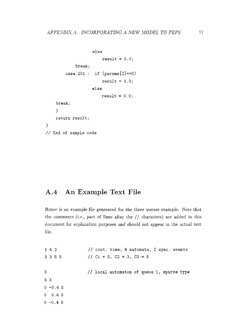
APPENDIX A. INCORPORATING A NEW MODEL TO PEPS I I
elseresult = 0.0;
break;case 201 : if (params[2]==0)
result = 1.0;else
result = 0.0;break;}return result;
>// End of sample code
A .4 An Example Text File
Below is an example file generated for the three queues example. Note that the comments (i.e., part of lines after the / / characters) are added to this document for explanation purposes and should not appear in the actual text file.
1 4 2 3 3 5 5
// cont. time, 4 automata, 2 sync, events // Cl = 3, C2 = 3, C3 = 5
0
4 30 -0.4 0 0 0.4 00 -0.4 0
// local automaton of queue 1, sparse type
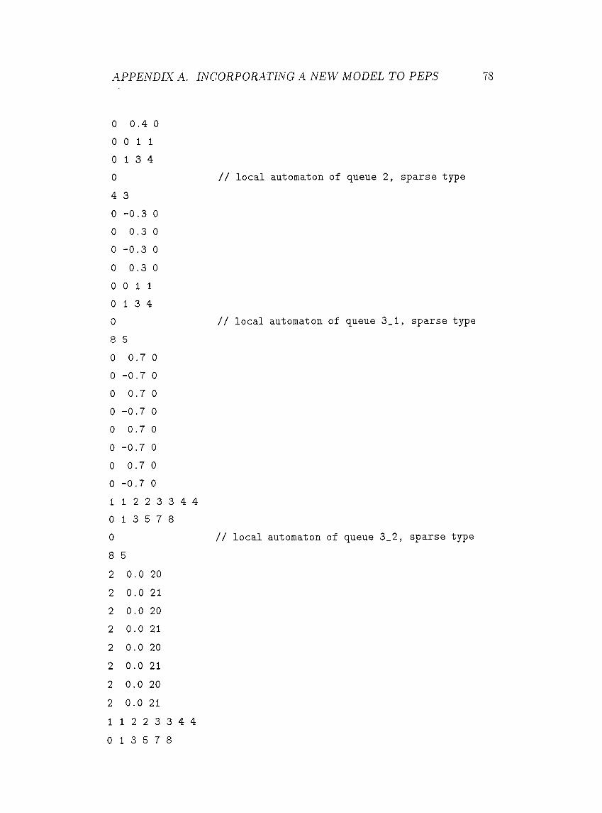
APPENDIX A. INCORPORATING A NEW MODEL TO PEPS 78
0 0.4 00 0 1 1
0 1 3 4 04 30 -0.3 0 0 0.3 00 -0.3 0 0 0.3 00 0 1 1
0 1 3 4 08 50 0.7 00 -0.7 0 0 0.7 00 -0.7 0 0 0.7 00 -0.7 0 0 0.7 00 -0.7 0 1 1 2 2 3 3 4 40 1 3 5 7 8 08 52 0.0 20 2 0. 0 21
2 0.0 20 2 0. 0 21
2 0.0 20 2 0. 0 21
2 0.0 20 2 0. 0 21
1 1 2 2 3 3 4 4 0 1 3 5 7 8
// local automaton of queue 2, sparse type
// local automaton of queue 3_1, sparse type
// local automaton of queue 3_2, sparse type
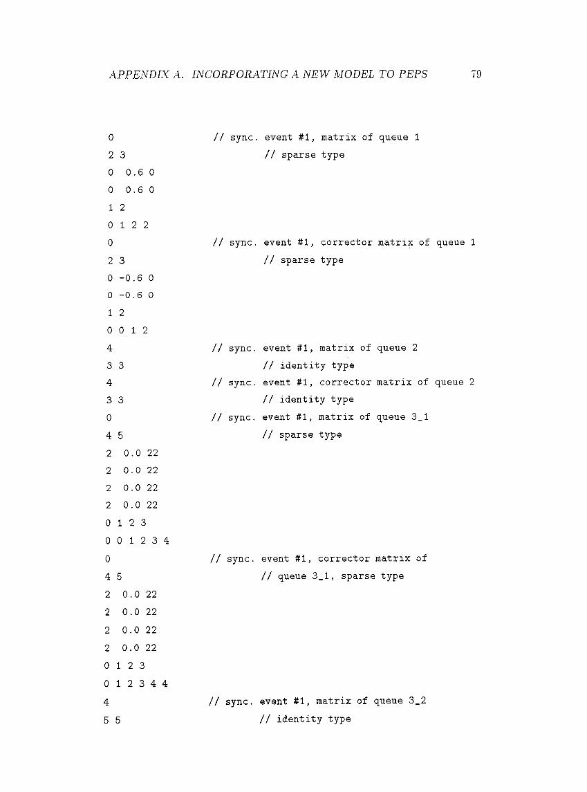
APPENDIX A. INCORPORATING A NEW MODEL TO PEPS 79
0
2 30 0. 6 0
0 0.6 0
1 2
0 1 2 2
0
2 30 -0.6 0 0 -0.6 0 1 2
0 0 1 2
43 343 3 04 52 0.0 222 0.0 222 0.0 222 0.0 220 1 2 3 0 0 1 2 3 40
4 52 0.0 222 0.0 222 0.0 22
2 0.0 220 1 2 3 0 1 2 3 4 445 5
// sync, event #1, matrix of queue 1 // sparse type
// sync, event #1, corrector matrix of queue 1 // sparse type
// sync, event #1, matrix of queue 2 // identity type
// sync, event #1, corrector matrix of queue 2 // identity type
// sync, event #1, matrix of queue 3_1 // sparse type
// sync, event #1, corrector matrix of // queue 3_1, sparse type
// sync, event #1, matrix of queue 3_2 // identity type
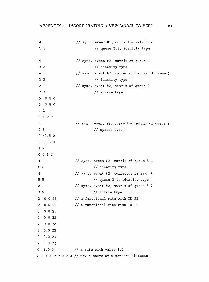
APPENDIX A. INCORPORATING A NEW MODEL TO PEPS 80
4 // sync, event #1, corrector matrix of5 5 // queue 3_2, identity type
4 // sync, event #2, matrix of queue 13 3 // identity type4 // sync, event #2, corrector matrix of3 3 // identity type0 // sync, event #2, matrix of queue 22 3 // sparse type0 0.5 00 0.5 01 20 1 2 20 // sync, event #2, corrector matrix of2 3 // sparse type0 -0.5 00 -0.5 01 20 0 1 24 // sync, event #2, matrix of queue 3_15 5 // identity type4 // sync, event #2, corrector matrix of5 5 // queue 3_1, identity type0 // sync, event #2, matrix of queue 3_29 5 // sparse type2 0.0 23 //a functional rate with ID 232 0.0 22 // a functional rate with ID 222 0.0 232 0.0 222 0.0 232 0.0 222 0.0 232 0.0 220 1.0 0 // a rate with value 1.00 0 1 1 2 2 3 3 4 / / row numbers of 9 nonzero elements
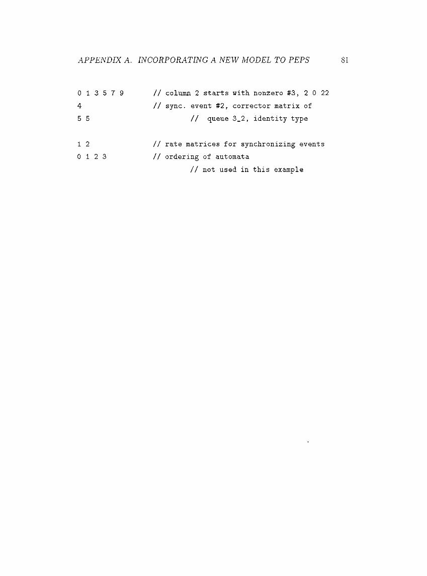
APPENDIX A. INCORPORATING A NEW MODEL TO PEPS 81
0 1 3 5 7 945 5
// column 2 starts with nonzero #3, 2 0 22 // sync, event #2, corrector matrix of
// queue 3_2, identity type
1 2
0 1 2 3// rate matrices for synchronizing events // ordering of automata
// not used in this example
Bibliography
[1] Benzi, M., and Dayar, T., “The arithmetic mean method for finding the stationary vector of Markov chains. ’ Parallel Algorithms and Applications. 6 (1995) 25-37.
[2] Davio, M., “Kronecker products and shuffle algebra." IEEE Transactions on Computers., C-30/2 (1981), 116-125.
[3] Dayar, T., Pentakalos, 0 . I., and Stephens, A. B., “ .Analytical modeling of robotic tape libraries using stochastic automata.” Technical Report TR- .97-1.98, CESDIS, NASA/GSFC (1997).
[4] Dianne, 0 . P., “Iterative methods for finding the stationary vector for Markov chains,” in: Linear Algebra, Markov Chains, and Queueing Mod
els. Springer-Verlag, Meyer, C., D., Plemmons, R.. .J.. eels.. New York, NY, (1993) 125-136.
[5] Fernandes, P., Plateau, B., and Stewart, W. .J., “Efficient descriptor- vector multiplications in stochastic automata networks.” INRIA Report # 2935. -Anonymous ftp ftp.inria.fr/INRI.A/Publication/RR.
[6] Fernandes, P., Plateau, B., and Stewart, W. .J.. “Numerical issues for stochastic automata networks,” in: PAPM 96, Eourth Process Algebras and Performance Modelling Workshop, Torino, Italy, .July 1996.
[7] Hageman, L., and Young, D., Applied Iterative Methods. Academic Press, New York, NY, 1981.
[8] Malhis, L. M., and Sanders, W. H., “An efficient two-stage iterative method for the steady-state analysis of Markov regenerative stochastic
Petri net models,” Performance Evaluation, '2 L·'28 (1996), 583-601.
82
BIBLIOGRAPHY 83
[9] Plateau, B., “On the stochastic structure of parallelism and synchronization models for distributed algorithms,” in: Proceedings of the SIGMET- RICS Conference on Measurement and Modelling o f Computer Systems, Austin, TX, August 1985, 147-154.
[10] Plateau, B., and Atif, K., “Stochastic automata network for modeling parallel systems,” IEEE Transactions on Software Engineering, 17/10 (1991)
1093-1108.
[11] Plateau, B., and Fourneau, .J. M., “A methodology for solving Markov models of parallel systems” , Journal of Parallel and Distributed Comput
ing, 12 (1991) 370-387
[12] Plateau, B., Fourneau, J. M., and K.-H. Lee, “PEPS: A package for solving complex Markov models of parallel systems,” in: Modeling Techniques and Tools for Computer Performance Evaluation, R. Puigjaner and D. Potier. eds., Spain, September 1988, 291-305.
[13] Saad, Y., and Schultz, M., H., “Conjugate gradient like algorithms for solving nonsymmetric linear systems,” Mathematics of Computation, 170 (1985) 417-424
[14] Semal, P., “Refinable Bounds for large Markov chains,” IEEE Transac
tions On Computers, 10 (1995) 1216-1222.
[15] Stewart, VV. J., MARCA: Markov Chain Analyzer, IEEE Computer Repos
itory No. R76 232, 1976.
[16] Stewart, W. introduction to the Numerical Solutions of Markov Chains, Princeton University Press, Princeton, N.J, 1994.
[17] Stewart, W. .J., Atif, K., and Plateau, B., “The numerical solution
of stochastic automata networks,” European Journal of Operational Re
search, 86 (1995) 503-525