IW, Princeton, Paper

8/6/2019 IW, Princeton, Paper

http://slidepdf.com/reader/full/iw-princeton-paper 1/26

Research Project : automatized discovery of

similarities, intertextuality and plagiarism in texts

Clement Canonne†

Adviser: David Mimno

May 14, 2011

Abstract

This paper examines a method to match texts (in a broad acception)according to their stylistic similarity, with standard clustering techniques,and considers for that purpose various means of quantifying the dissimi-larity between texts. A comparison of those criteria - derived from well-known measures such as weighted Euclidean distances or Bray-Curtis dis-similarity - is then undergone, and an analysis of the results the afore-mentioned method yields is attempted.

Acknowledgements

I would like to thank Pr. S.Y.Kung, without whom my notions of machine learning would have been far blurrier; and express my gratitude

to my adviser, David Mimno, without whose help, advice and suggestionsthis paper would have been nothing but “a tale full of sound and fury,

signifying nothing”. Yet much faster to write.

†This work has been conducted in the Princeton University, both as part of a Senior In-

dependent Work (COS498), and within the context of the course Digital Neurocomputing

(ELE571).

1



Contents

1 Introduction 31.1 Overview . . . . . . . . . . . . . . . . . . . . . . . . . . . . . . . 3

2 Applications 3

3 Approach 33.1 Summary: protocol . . . . . . . . . . . . . . . . . . . . . . . . . . 33.2 Clustering algorithm: K-Means . . . . . . . . . . . . . . . . . . . 43.3 Features . . . . . . . . . . . . . . . . . . . . . . . . . . . . . . . . 53.4 Corpus . . . . . . . . . . . . . . . . . . . . . . . . . . . . . . . . . 63.5 Presentation of the metrics . . . . . . . . . . . . . . . . . . . . . 73.6 How to compare clusterings . . . . . . . . . . . . . . . . . . . . . 9

3.6.1 Variation of information . . . . . . . . . . . . . . . . . . . 93.6.2 Similarity matrices . . . . . . . . . . . . . . . . . . . . . . 93.7 Classification of new samples . . . . . . . . . . . . . . . . . . . . 10

4 Results 104.1 Clustering comparison: Variation of information . . . . . . . . . 124.2 Text matchings . . . . . . . . . . . . . . . . . . . . . . . . . . . . 14

5 Future work 19

6 Conclusion 20

7 Appendix 21

7.1 Complete list of features . . . . . . . . . . . . . . . . . . . . . . . 217.2 Metrics summary . . . . . . . . . . . . . . . . . . . . . . . . . . . 227.2.1 Description . . . . . . . . . . . . . . . . . . . . . . . . . . 227.2.2 Converting similarity measures in pseudo-semi-distances . 237.2.3 About the Extended Jaccard index . . . . . . . . . . . . . 25

2



1 Introduction

1.1 Overview

This project aims at finding a way, given a set of texts (that is, novels, shortstories, plays, and articles), to detect intertextuality (or, in a broader sense,similarities) between them, by using machine learning techniques. Before goingfurther, let us state precisely what actual meaning of “similarity” is considered.Two texts can indeed be related in many ways:

- Common (thematic) structure (narrative patterns, such as in tales ormyths...)

- Variations upon a plot: for example, Antigone (by Sophocle, Anouilh,Brecht, Cocteau. . . )

- Concepts (when two articles or books share so many concepts that they

should be related): e.g, philosophy books about ethics- Style: either between books by the same author 1 or in the case of pastiches

(texts written a la maniere de).

- Shared vocabulary/chunks of sentences: for example, in the case of pla-giarism, a lot of words or collocations are common to both texts

Within the framework of this project, we shall focus on the style, that is, thespecificities in grammar, syntax, punctuation, rythm of sentences, use of vo-cabulary, . . . constituting the “signature” of an author, and making its workrecognizable.

2 Applications

We develop here an automated method to find out which books are similar,from a stylistic point of view; it will not (and, for that matter, is not meantto) replace human judgment in such comparisons, but hopefully be an auxiliaryand complementary tool for that purpose, allowing to “prune” the possibilitiesbefore a human eye investigate further, focusing on the most likely matches.

Besides, this technique could also be applied in two other areas: the firstone is plagiarism detection , where a positive match between two texts’ stylewould be related to a possible copying, and be a preliminary test before further,in-depth, inquiries. The second would be authorship controversies, where, givenan unknown work, one tries to find out whom is the likeliest author.

3 Approach

3.1 Summary: protocol

As outlined above, this work focuses on clustering texts (in a broad sense)according to their style. The first task is thus to pick a set of features, fromeach text, which could accurately characterize it in that view.

Before that, let us specify that by text , is meant any written English work,whether in verse or prose, but not scientific formulas nor source code. In other

1Even if it is not explicit, as in the case of authors using pseudonyms, like RomainGary/Emile Ajar.

3



terms, the work must be either literary or, at least, proper written English (so

that any consideration of written style can actually apply).

Protocol: Here is the summary of the different steps involved in this approach,and a brief description of each of them:

(i) Downloading all the Project Gutenberg (PG)2texts, and preprocess themby removing the extra PG header and footer (added by the PG volunteersin every work they digitalize), and discarding books whose length was lessthan 16750 bytes (this threshold, arbitrary chosen, correspond to workswhose length does not exceed approximatively 4-6 pages - indeed, the riskwas that with such short texts, the residual “noise” due to remaining tagsof words added by the PG might have skewed the results)

(ii) Processing them, extracting the features (cf. Section 3.3 below) from eachtext (using, amongst others, parser and named entity recognizer (NER)from the Stanford NLP Tools)3.

(iii) Shuffling the corpus to avoid (when sampling the corpus for a training set)bias due to consecutive, too similar, texts (e.g., if works were grouped byauthor in the original PG directories)

(iv) Running with different metrics (see Section 3.5, page 7, for a description),on a training set of 500 samples4, with the same algorithm (K-Means - cf Section 3.2) and parameters (max. 100 iterations per run, K max = 99,random initialization)

(v) Analyzing the clusterings obtained with K-Means, comparing the rele-

vance of each metric, and finding a way to combine the most relevantcriteria.

3.2 Clustering algorithm: K-Means

K-Means is an unsupervised clustering algorithm (that is, a clustering algorithmworking on an unlabeled training dataset - without “teacher” values specifyingwhat should be the optimal output on the training vectors), whose objectiveis to partition the N training vectors (from the training dataset X ) into K max

different clusters, where K max is a given parameter.K-Means works by maintaining and updating K max different centroid centers

µk ∈ RM , and minimizing the sum-of-squared-distances E of each point to the

center of the cluster Ck it belongs to:

E (X ) =

Kmaxk=1

x∈Ck

x − µk 2

2The Project Gutenberg is a volunteer project whose goal is to make freely available digi-talized works (eBooks,. . . ): http://www.gutenberg.org

3“The Natural Language Processing Group at Stanford University is a team of faculty,research scientists, postdocs, programmers and students who work together on algorithms thatallow computers to process and understand human languages”: http://nlp.stanford.edu

4Mainly because of time constraints, using more samples was discarded as it would havegreatly increased the processing time required.

4

http://www.gutenberg.org/

http://nlp.stanford.edu/

http://nlp.stanford.edu/

http://www.gutenberg.org/



Given a maximum number of iterations I max, K-Means, at each iteration, assign

each vector x to the cluster whose centroid center is the closest; at the end of each iteration, each centroid center µk is updated to be the barycenter of allvector contained in the kth cluster [2].

The original centroid locations are generally picked randomly; K-Means,when it converges within the maximum number of iterations allowed, outputsa clustering whose value E (X ) is a local minimum of E ; note that this localminimum depends on the initialization (two different initial configurations of the centroids may result in different clusterings, both local minima of the costfunction). Furthermore, K-Means, like all clustering algorithms, is heavily de-pendent on the metric used - fact this study is based upon.

3.3 Features

From each text (sample), a set of characteristics was extracted, mapping eachof them to a vector in R

M . In order to capture the most possible stylisticinformation, several aspects were considered (see Appendix 7.1 for an exhaustivelist and description of the features):

words statistics (ws): for each word from a reference dictionary, indicatorsare computed to quantify the density of this word in the text, both relativeto the text and to what was expected relatively to its usual frequency. 5

named entities (ne): the overall frequency of named entities, such as names,cities, institutions (3 values)

sentence splitting (ss): statistics about the length of sentences (minimum,maximum, average and standard deviation) (4 values)

chapter splitting (cs): statistics about the length of chapters (4 values)

punctuation (pn): frequency of each punctuation sign, and overall punctua-tion frequency compared to the text character count. . . (17 values)

lexical categories (lc): frequency of each category (adjectives, nouns, verbs,adverbs. . . ) in the text, compared to the number of words (7 values)

All these values have then been normalized, to prevent any scale effect (due todifferent, non-comparable, range of values for two different features):

vi ←vi − vi

σ(vi)

where σ(vi) and vi are respectively the empirical standard deviation and meanfor the ith feature, over all samples.

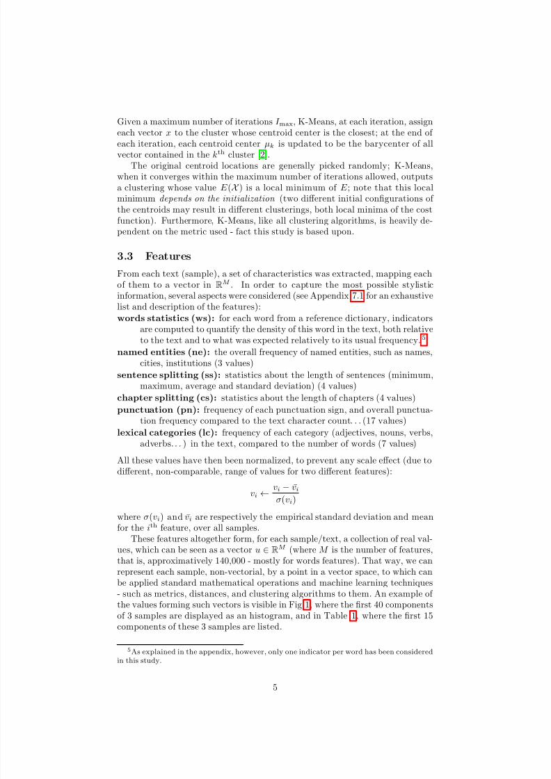
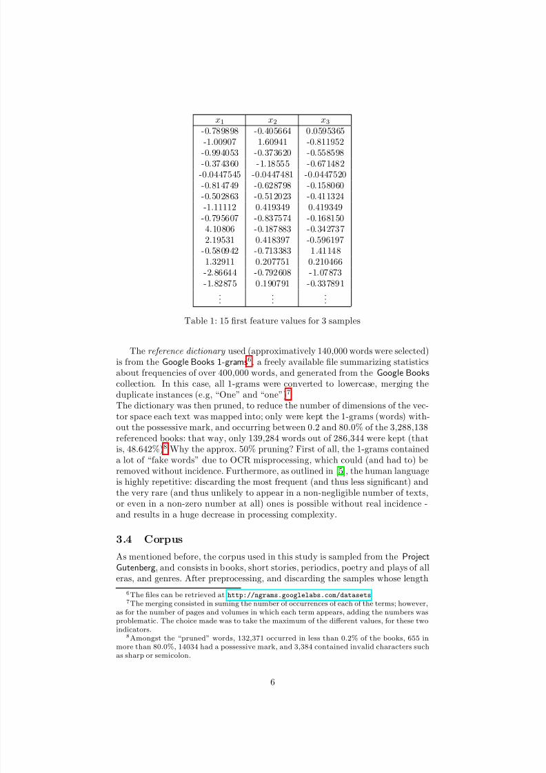
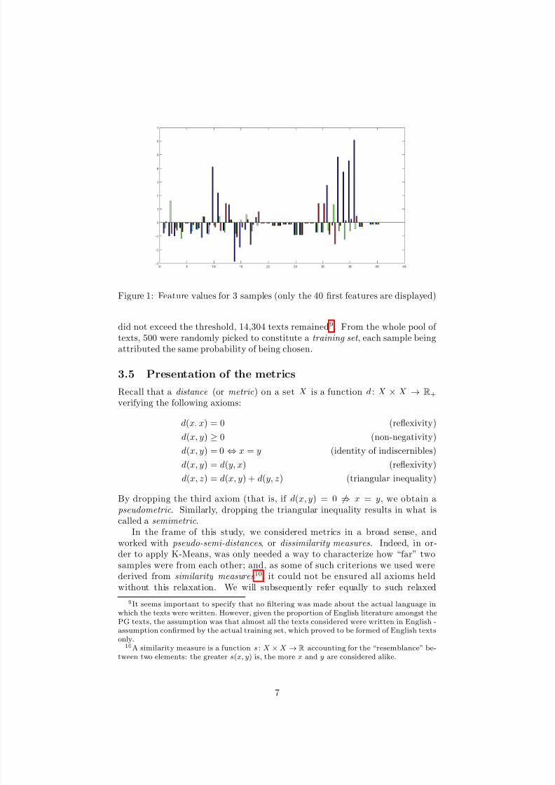
These features altogether form, for each sample/text, a collection of real val-ues, which can be seen as a vector u ∈ RM (where M is the number of features,that is, approximatively 140,000 - mostly for words features). That way, we canrepresent each sample, non-vectorial, by a point in a vector space, to which canbe applied standard mathematical operations and machine learning techniques- such as metrics, distances, and clustering algorithms to them. An example of the values forming such vectors is visible in Fig.1, where the first 40 componentsof 3 samples are displayed as an histogram, and in Table 1, where the first 15components of these 3 samples are listed.

5As explained in the appendix, however, only one indicator per word has been consideredin this study.

5



x1 x2 x3

-0.789898 -0.405664 0.0595365-1.00907 1.60941 -0.811952-0.994053 -0.373620 -0.558598-0.374360 -1.18555 -0.671482

-0.0447545 -0.0447481 -0.0447520-0.814749 -0.628798 -0.158060-0.502863 -0.512023 -0.411324-1.11112 0.419349 0.419349

-0.795607 -0.837574 -0.1681504.10806 -0.187883 -0.3427372.19531 0.418397 -0.596197

-0.580942 -0.713383 1.411481.32911 0.207751 0.210466

-2.86644 -0.792608 -1.07873-1.82875 0.190791 -0.337891

......

...

Table 1: 15 first feature values for 3 samples

The reference dictionary used (approximatively 140,000 words were selected)is from the Google Books 1-grams6, a freely available file summarizing statisticsabout frequencies of over 400,000 words, and generated from the Google Bookscollection. In this case, all 1-grams were converted to lowercase, merging theduplicate instances (e.g, “One” and “one”)7

The dictionary was then pruned, to reduce the number of dimensions of the vec-tor space each text was mapped into; only were kept the 1-grams (words) with-out the possessive mark, and occurring between 0.2 and 80.0% of the 3,288,138referenced books: that way, only 139,284 words out of 286,344 were kept (thatis, 48.642%)8 Why the approx. 50% pruning? First of all, the 1-grams containeda lot of “fake words” due to OCR misprocessing, which could (and had to) beremoved without incidence. Furthermore, as outlined in [5], the human languageis highly repetitive: discarding the most frequent (and thus less significant) andthe very rare (and thus unlikely to appear in a non-negligible number of texts,or even in a non-zero number at all) ones is possible without real incidence -and results in a huge decrease in processing complexity.

3.4 CorpusAs mentioned before, the corpus used in this study is sampled from the ProjectGutenberg, and consists in books, short stories, periodics, poetry and plays of alleras, and genres. After preprocessing, and discarding the samples whose length

6The files can be retrieved at http://ngrams.googlelabs.com/datasets7The merging consisted in suming the number of occurrences of each of the terms; however,

as for the number of pages and volumes in which each term appears, adding the numbers wasproblematic. The choice made was to take the maximum of the different values, for these twoindicators.

8Amongst the “pruned” words, 132,371 occurred in less than 0.2% of the books, 655 inmore than 80.0%, 14034 had a possessive mark, and 3,384 contained invalid characters suchas sharp or semicolon.

6

http://ngrams.googlelabs.com/datasets

http://ngrams.googlelabs.com/datasets



Figure 1: Feature values for 3 samples (only the 40 first features are displayed)

did not exceed the threshold, 14,304 texts remained9. From the whole pool of texts, 500 were randomly picked to constitute a training set , each sample beingattributed the same probability of being chosen.

3.5 Presentation of the metrics

Recall that a distance (or metric) on a set X is a function d : X × X → R+

verifying the following axioms:

d(x, x) = 0 (reflexivity)

d(x, y) ≥ 0 (non-negativity)

d(x, y) = 0 ⇔ x = y (identity of indiscernibles)

d(x, y) = d(y, x) (reflexivity)

d(x, z) = d(x, y) + d(y, z) (triangular inequality)

By dropping the third axiom (that is, if d(x, y) = 0 ⇒ x = y, we obtain apseudometric. Similarly, dropping the triangular inequality results in what iscalled a semimetric.

In the frame of this study, we considered metrics in a broad sense, andworked with pseudo-semi-distances, or dissimilarity measures. Indeed, in or-der to apply K-Means, was only needed a way to characterize how “far” twosamples were from each other; and, as some of such criterions we used werederived from similarity measures10, it could not be ensured all axioms heldwithout this relaxation. We will subsequently refer equally to such relaxed

9It seems important to specify that no filtering was made about the actual language inwhich the texts were written. However, given the proportion of English literature amongst thePG texts, the assumption was that almost all the texts considered were written in English -assumption confirmed by the actual training set, which proved to be formed of English textsonly.10A similarity measure is a function s : X × X → R accounting for the “resemblance” be-

tween two elements: the greater s(x, y) is, the more x and y are considered alike.

7



metrics as pseudo-semi-distances, pseudo-semi-metrics, dissimilarity measures

or even, simply, metrics.Here is a list of the different measures the K-Means algorithm was ran with:

Weighted Euclidean distance This is a generalized version of the Euclideandistance (also called norm 2 ), resulting in a pseudometric.with several setsof different non-negative weights (ωi)1≤i≤M for the features:

(i) First set: ωi = 0.01 on the ws, ωi = 10 on the cs11, ωi = 10 onthe min and max sentence length features (for the same reason asthe cs) and ωi = 1000 on other indicators. Emphasis is thus puton the global stylistic indicators, and the frequencies of the wordsthemselves have less impact on the decision.

(ii) Second set: same weights, but with ωi = 0 on the ws. The word

distribution is completely ignored.(iii) Third set: ωi = 1 on the punctuation (pn) and the sentence length

average and standard deviation, and 0 on the rest of the features:emphasis is put on the splitting and rythm of the language.

(iv) Fourth set: ωi = 1 on the ne and lc indicators, and 0 on the rest:emphasis is put on the use of names and syntax.

(v) Fifth set: ωi = 1 on the pn and lc indicators, and 0 on the rest:emphasis is put on the use of punctuation and syntax.

Weighted Manhattan distance This is a generalized version of the Manhat-tan distance (also called Variational , City block or norm 1 ), producing apseudometric. The weight sets used are the same as before.

χ2 (Chi-square) distance Pearson’s χ2 statistics test can be generalized as ametric between two samples (real-valued vectors), resulting in this distance

Weighted Chi-square with the same weight sets as previously. Note that the“regular” χ2 just correspond to uniform weights ωi = 1 ∀i.

Canberra distance first introduced (and then slightly modified) by Lance & Williams([3], [4]), this is a metric well-suited to values centered on the origin: in-deed, in the form due to Adkins, described in [4], the result “becomesunity when the variables are of opposite sign.”12 It is thus a good indica-tor when interested in dividing data according to a threshold value.

Weighted Canberra , again with the 5 weight sets.

Bray-Curtis dissimilarity (it is a semimetric) this criterion originates frombiology and botany, as a value reflecting the difference of composition (interm of species) between two sites

Weighted Bray-Curtis again with the 5 same weight sets.

11Chapter statistics were considered less reliable than other global indicators - and wereconsequently given a smaller weight - since the chapter splitting tended to be somehow. . . fuzzyin some texts of PG.12Cf. Jan Schulz, http://www.code10.info/index.php?option=com_content&view=

article&id=49:article_canberra-distance&catid=38:cat_coding_algorithms_

data-similarity&Itemid=57

8

http://www.code10.info/index.php?option=com_content&view=article&id=49:article_canberra-distance&catid=38:cat_coding_algorithms_data-similarity&Itemid=57








Cosine dissimilarity adapted from the Cosine similarity measure, which quan-

tifies the “angle” between to vectors inRM

(the smaller the angle is, themore the two vectors are alike).

Extended Jaccard dissimilarity derived from the Extended Jaccard simi-larity measure (something referred to as the Tanimoto coefficient ), a gen-eralized version of an indice quantifying the degree of overlapping betweentwo sets.

For a more in-depth description of those measures, and how similarity mea-sures were converted in pseudo-semi-distances, refer to Appendix 7.2. Note thatother measures could have been used, such as Mahalanobis distances, PearsonCorrelation measure, or Dice similarity coefficient. The first former were dis-carded as too computationally intense, while the latter is equivalent to the

extended Jaccard coefficient

13

.

3.6 How to compare clusterings

3.6.1 Variation of information

The Variation of Information (VI), introduced in [7], is a metric on the spaceof clusterings, characterizing the quantity of information lost or gained whenswitching from a clustering to another (on the same dataset). Its propertiesmake it an useful tool to cluster the clusterings themselves, or, in other terms,to find out which clusterings are the more alike.

For two clusterings C = (C k)1≤k≤K , C = (C k)1≤k≤K on a set of n datapoints, the variation of information is defined as

V I (C, C) = H (C) + H (C) − 2I (C, C)

where the entropy H , the mutual information I and the cluster probabilitiesP, P are given by

H (C) = −Kk=1

P (k)log P (k) ≥ 0, I (C, C) =

Kk=1

K=1

P (k, )logP (k, )

P (k)P ()≥ 0

and

P (k, ) =|C k ∩ C |

n, P (k, ) =

|C k |

n, P () =

|C |

n

In this case, this criterion was applied to the clusterings obtained by runningK-Means on the training data set, with the 29 different metrics (see Section 4.1,p.12, for the results and their analysis).

3.6.2 Similarity matrices

The clustering algorithm’s output consists, for each of the metrics, in a 99 ×500clustering matrix C, whose (i, j) component reflects the appartenance of the jth

13That is, one can convert Jaccard measure into Dice’s one with the strictly increasingmapping h : x → 2x

1+x, x > −1.

9



sample to the ith cluster14.

From this matrix can be derived, for each clustering, a 500 × 500 symmetricsimilarity matrix S = (sij), with

sij =

1, if the ith and jth sample belong to the same cluster

0 otherwise

From these 29 similarity matrices, could then be computed the average sim-ilarity matrix S and the standard deviation of similarity matrix Σ - that is,respectively, the matrix of mean and standard deviation of the pairwise similar-ities. As we will see in Section 4.2, these two matrices constitute a good start tofind out the most likeliest matches between texts; indeed, two samples with veryhigh average similarity and very standard deviation are, with high probability,stylistically related in some way.

3.7 Classification of new samples

More than a clustering of the provided samples, K-Means outputs as well thecentroids of each cluster, as points µk ∈ RM (1 ≤ k ≤ K max). With thesetrained centroids, it becomes possible to proceed to online classification of newsamples: given a sample (not belonging to the training set), mapped to a vectorx ∈ R

M , we can determine the most likely group it belongs by choosing thenon-emptycluster k∗ to which it is the closest; that is,

k∗ = argmink:Ck=∅

d(x, µk)

where d is the pseudo-semi-distance associated to the clustering.

This possibility is mentioned as an important possible development; however,we lacked time to test such online classification on other samples from the poolof texts, and was therefore not able to assert how it actually performs on suchnew samples. To go further, it would be interesting to quantify what woulda “good number” of training samples (500, in the case of this study) be, andhow to combine the different clusterings (derived from the 29 measures, withdifferent numbers of non-empty clusters, different cluster centroids, and differentassociated metrics) to achieve optimal classification.

4 Results

Convergence of the clusterings Interestingly enough, when running K-Means,the required time was hugely dependent on the dissimilarity measures consid-ered. While most of the measures ensured a rather quick convergence of thealgorithm (between 8 and 29 iterations for the weighted Euclidean metrics,between 21 and 32 for the Bray-Curtis ones, between 31 and 40 for the fiveCanberra (one of the slowest to converge), 5 or 6 iterations for the Cosine andextended Jaccard, and 10 for Chi-square - the maximum authorized number

14K-Means being a hard clustering technique, each sample belongs to one and only onecluster, and ci,j ∈ {0, 1}. For other types of clusterings, the values would have been non-negative, fractional, each column suming up to 1 ( soft clusterings).

10



being 100), some other metrics failed to converge in the allowed time. In partic-

ular, the weighted Manhattan metrics either converged very fast (in 4, 4 and 2iterations, respectively for the first, second and fourth set of weights) or failed toconverge at all, resulting in trivial (only one non-empty cluster) or almost-trivialclusterings - that is, a cluster of 499 points, and one of only one sample. Thiswas the case for the third and fifth set of weights, again with the Manhattanmeasure - in other terms, the two set of weights putting a lot of emphasize onthe punctuation.

As for the weighted Chi-square measure, it never converged in less than100 iterations. However, the resulting clusterings were not trivial (or almost)ones, and consisted in more than 50 non-empty clusters (of between 1 and 20samples).

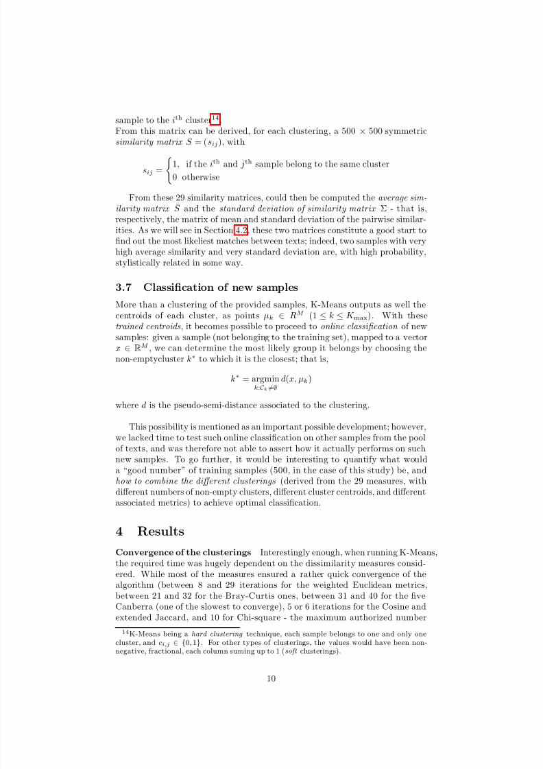
Figure 2: Variation of information between the only non-trivial Bray-Curtisclustering and the 28 others

The analysis of the clusterings furthermore show that the Bray-Curtis dis-similarity measures gave very poor results, with trivial clusterings for either thenon-weighted one and all set of weights - except for the third one (the one focus-ing on punctuation and length of sentences: cf. Fig.2 for a vizualization of itsdistance to other clusterings). This strongly advocates for the droppingof the Bray-Curtis measure in such tasks - as outlined below, the resultsit gives are very similar to other metrics, and, unless punctuation is to be themain criterion, the computational cost involved by adding a metric to the poolis not worth it.

11



(a) W.r.t. clustering 10 (b) W.r.t. clustering 13

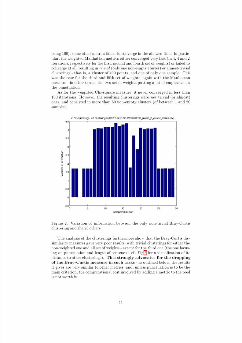
Figure 3: Example of pairwise comparisons (VI) between clusterings.

4.1 Clustering comparison: Variation of information

For our purpose, was computed, for each metrics, the variation of informationbetween the resulting clustering and the 29 others. The result is illustrated inFig.3, by two examples15. This produced a symmetric, 29× 29 matrix V I (i, j).To visualize the result, we used the Matlab function mdscale to approximatethe dissimilarity matrix in 2 and 3 dimensions16

Multidimensional scaling Here is briefly recalled the principle of (non-classical) multidimensional scaling, performed by the previously mentioned Mat-lab function. As developed in [8], it aims at representing a set of points from ahigh-dimensional space into a lower dimensional, “easier-to-grasp”, space (typi-cally, 2 or 3 when the purpose is to visualize data distribution) while preservingas much as possible the distances between those points - that is, in such a fashionthat the resulting distances are monotonically related to the original pointwisedistances. Given a N × N pointwise dissimilarity matrix (d∗ij), mdscale thusproduces a N × d matrix, whose rows are the coordinates of the mapped pointsin the destination d-dimensional space. The most common criterion to evaluatethe goodness of the mapping, introduced by Kruskal in 1964, is called stress(the smaller stress, the better), and is defined as

s =

1≤i,j≤N f (d∗

ij) − d

ij2

1≤i,j≤N

d2ij

where the dij are the (Euclidean) distances between the points in the targetspace, and f (d∗ij) are the best-fitting distances corresponding to the input dis-

15Note that the clusterings 1, 2, 4, 5, 6, 25, 26 and 28 were trivial ones.16For that purpose, we had to remove the identical clusterings in order to get a nonsingular

VI matrix; indeed, 8 metrics resulting in the same, trivial clustering (all data points in thesame cluster) - they were replaced by only one instance of that trivial clustering.

12



similarities (found by monotonic regression, in order to minimize the stress)17.

(a) In two dimensions (b) In three dimensions

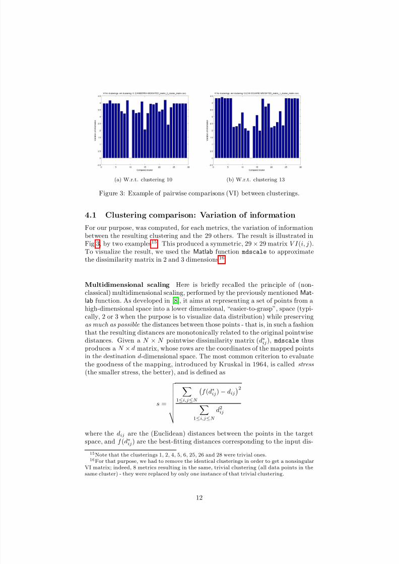
Figure 4: Multidimensional scaling of the VI (visualization)

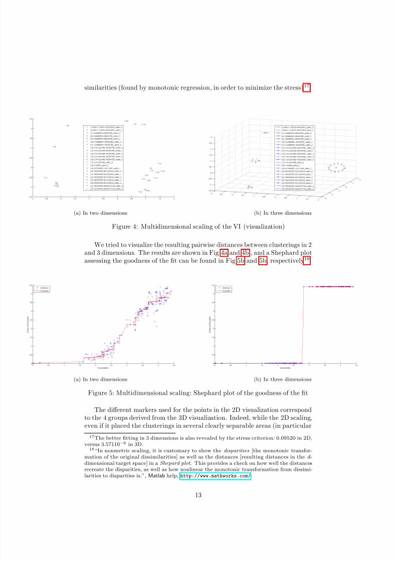
We tried to visualize the resulting pairwise distances between clusterings in 2and 3 dimensions. The results are shown in Fig.4a and 4b , and a Shephard plotassessing the goodness of the fit can be found in Fig.5b and 5b, respectively18

(a) In two dimensions (b) In three dimensions

Figure 5: Multidimensional scaling: Shephard plot of the goodness of the fit

The different markers used for the points in the 2D visualization correspondto the 4 groups derived from the 3D visualization. Indeed, while the 2D scaling,even if it placed the clusterings in several clearly separable areas (in particular

17The better fitting in 3 dimensions is also revealed by the stress criterion: 0.09520 in 2D,versus 3.57110−6 in 3D.18“In nonmetric scaling, it is customary to show the disparities [the monotonic transfor-

mation of the original dissimilarities] as well as the distances [resulting distances in the d-dimensional target space] in a Shepard plot . This provides a check on how well the distancesrecreate the disparities, as well as how nonlinear the monotonic transformation from dissimi-larities to disparities is.”, Matlab help, http://www.mathworks.com/

13

http://www.mathworks.com/

http://www.mathworks.com/



Number Measure Number Measure

1 Bray-Curtis (Weights 1) 7 Canberra (Weights 1)3 Bray-Curtis (Weights 3) 8 Canberra (Weights 2)17 Chi-Square (Unweighted) 9 Canberra (Weights 3)27 Manhattan (Weights 3) 11 Canberra (Weights 5)29 Manhattan (Weights 5) 12 Chi-Square (Weights 1)

13 Chi-Square (Weights 2)10 Canberra (Weights 4) 14 Chi-Square (Weights 3)15 Chi-Square (Weights 4) 16 Chi-Square (Weights 5)23 Euclidean (Weights 4) 20 Euclidean (Weights 1)

21 Euclidean (Weights 2)18 Cosine 22 Euclidean (Weights 3)19 Extended Jaccard 24 Euclidean (Weights 5)

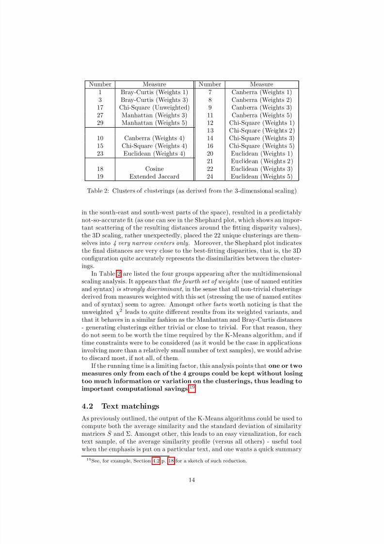
Table 2: Clusters of clusterings (as derived from the 3-dimensional scaling)

in the south-east and south-west parts of the space), resulted in a predictablynot-so-accurate fit (as one can see in the Shephard plot, which shows an impor-tant scattering of the resulting distances around the fitting disparity values),the 3D scaling, rather unexpectedly, placed the 22 unique clusterings are them-selves into 4 very narrow centers only. Moreover, the Shephard plot indicatesthe final distances are very close to the best-fitting disparities, that is, the 3Dconfiguration quite accurately represents the dissimilarities between the cluster-ings.

In Table 2 are listed the four groups appearing after the multidimensionalscaling analysis. It appears that the fourth set of weights (use of named entitiesand syntax) is strongly discriminant , in the sense that all non-trivial clusteringsderived from measures weighted with this set (stressing the use of named entitesand of syntax) seem to agree. Amongst other facts worth noticing is that theunweighted χ2 leads to quite different results from its weighted variants, andthat it behaves in a similar fashion as the Manhattan and Bray-Curtis distances- generating clusterings either trivial or close to trivial. For that reason, theydo not seem to be worth the time required by the K-Means algorithm, and if time constraints were to be considered (as it would be the case in applicationsinvolving more than a relatively small number of text samples), we would adviseto discard most, if not all, of them.

If the running time is a limiting factor, this analysis points that one or twomeasures only from each of the 4 groups could be kept without losing

too much information or variation on the clusterings, thus leading toimportant computational savings.19

4.2 Text matchings

As previously outlined, the output of the K-Means algorithms could be used tocompute both the average similarity and the standard deviation of similaritymatrices S and Σ. Amongst other, this leads to an easy vizualization, for eachtext sample, of the average similarity profile (versus all others) - useful toolwhen the emphasis is put on a particular text, and one wants a quick summary

19See, for example, Section 4.2 p. 18 for a sketch of such reduction.

14



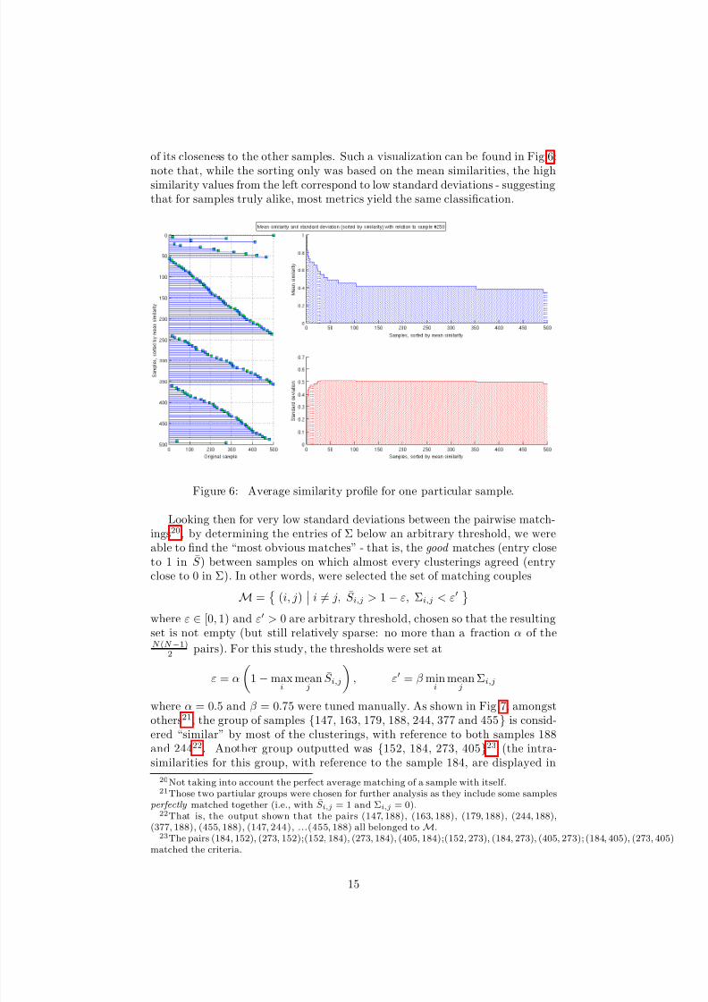
of its closeness to the other samples. Such a visualization can be found in Fig.6:

note that, while the sorting only was based on the mean similarities, the highsimilarity values from the left correspond to low standard deviations - suggestingthat for samples truly alike, most metrics yield the same classification.

Figure 6: Average similarity profile for one particular sample.

Looking then for very low standard deviations between the pairwise match-ings20, by determining the entries of Σ below an arbitrary threshold, we wereable to find the “most obvious matches” - that is, the good matches (entry closeto 1 in S ) between samples on which almost every clusterings agreed (entryclose to 0 in Σ). In other words, were selected the set of matching couples

M =

(i, j) i = j, S i,j > 1 − ε, Σi,j < ε

where ε ∈ [0, 1) and ε > 0 are arbitrary threshold, chosen so that the resultingset is not empty (but still relatively sparse: no more than a fraction α of theN (N −1)

2pairs). For this study, the thresholds were set at

ε = α

1 −max

imean

jS i,j

, ε = β min

imean

jΣi,j

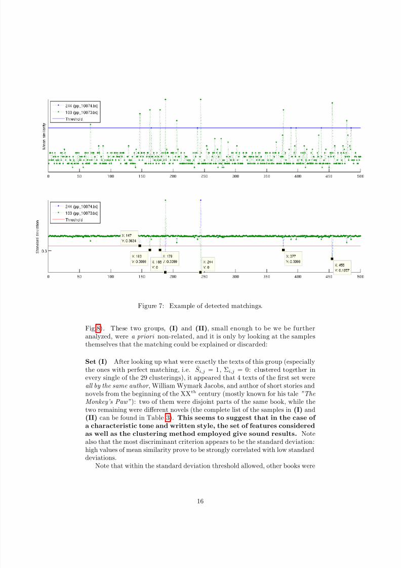
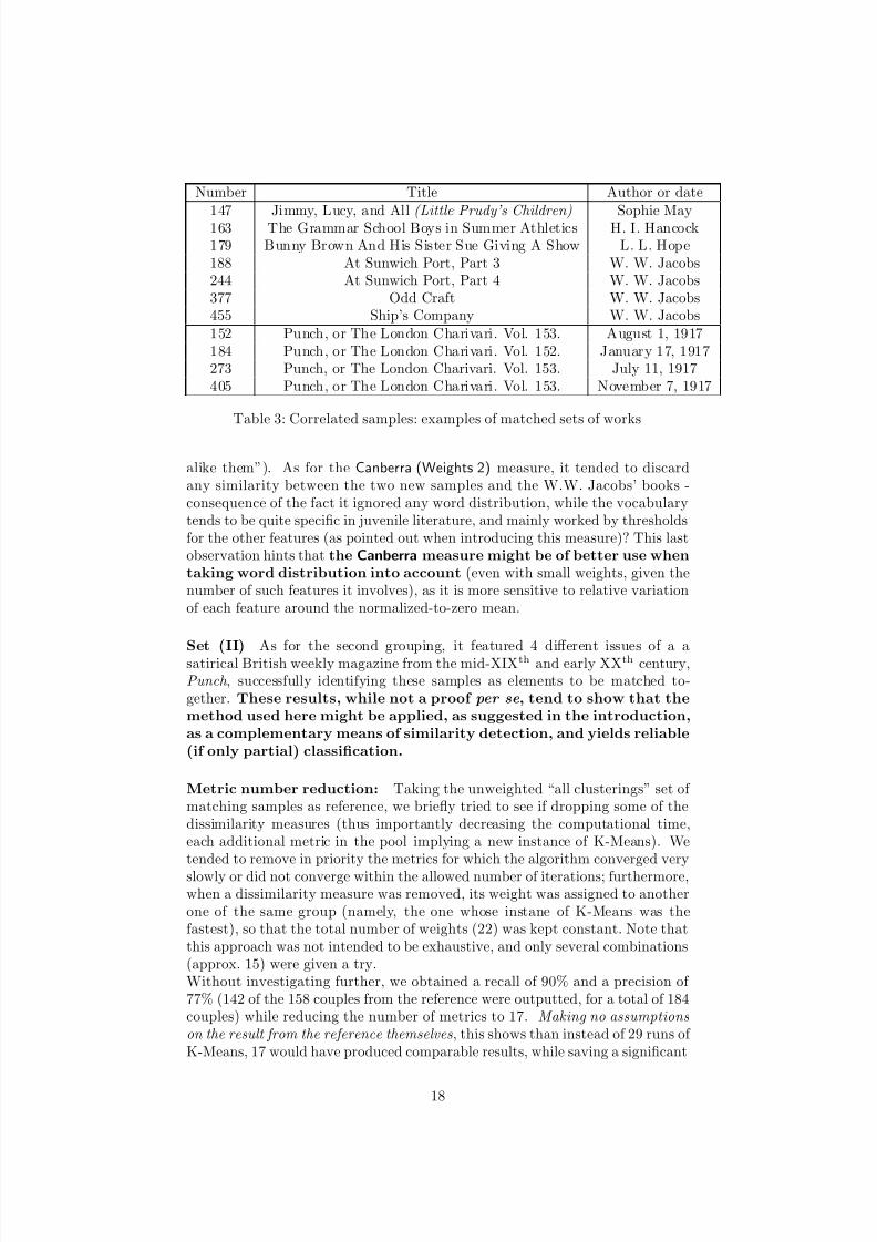
where α = 0.5 and β = 0.75 were tuned manually. As shown in Fig.7, amongstothers21, the group of samples {147, 163, 179, 188, 244, 377 and 455} is consid-ered “similar” by most of the clusterings, with reference to both samples 188and 24422. Another group outputted was {152, 184, 273, 405}23 (the intra-similarities for this group, with reference to the sample 184, are displayed in

20Not taking into account the perfect average matching of a sample with itself.21Those two partiular groups were chosen for further analysis as they include some samples

perfectly matched together (i.e., with S i,j = 1 and Σi,j = 0).22That is, the output shown that the pairs (147, 188), (163, 188), (179, 188), (244, 188),

(377, 188), (455, 188), (147, 244), ...(455, 188) all belonged to M.23The pairs (184, 152), (273, 152);(152, 184), (273, 184), (405, 184);(152, 273), (184, 273), (405, 273); (184, 405), (273, 405)

matched the criteria.

15





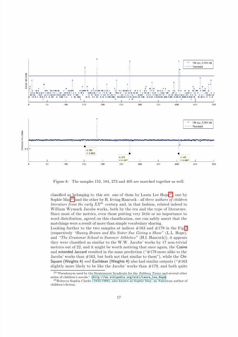
Figure 8: The samples 152, 184, 273 and 405 are matched together as well.

classified as belonging to this set: one of them by Laura Lee Hope24, one bySophie May25 and the other by H. Irving Hancock - all three authors of children literature from the early XX th century and, in that fashion, related indeed toWilliam Wymark Jacobs works, both by the era and the type of literature.Since most of the metrics, even those putting very little or no importance toword distribution, agreed on this classification, one can safely assert that thematchings were a result of more than simple vocabulary sharing.Looking further to the two samples at indices #163 and #179 in the Fig.7(respectively “Bunny Brown and His Sister Sue Giving a Show” (L.L. Hope),

and “The Grammar School in Summer Athletics” (H.I. Hancock)), it appearsthey were classified as similar to the W.W. Jacobs’ works by 17 non-trivialmetrics out of 22, and it might be worth noticing that once again, the Cosineand extended Jaccard resulted in the same prediction (“#179 more alike to theJacobs’ works than #163, but both not that similar to them”), while the Chi-Square (Weights 4) and Euclidean (Weights 4) also had similar outputs (“#163slightly more likely to be like the Jacobs’ works than #179, and both quite

24“Pseudonym used by the Stratemeyer Syndicate for the Bobbsey Twins and several otherseries of children’s novels.” (http://en.wikipedia.org/wiki/Laura_Lee_Hope)25Rebecca Sophia Clarke (1833-1906), also known as Sophie May, an American author of

children’s fiction.

17

http://en.wikipedia.org/wiki/Laura_Lee_Hope





Number Title Author or date

147 Jimmy, Lucy, and All (Little Prudy’s Children) Sophie May163 The Grammar School Boys in Summer Athletics H. I. Hancock179 Bunny Brown And His Sister Sue Giving A Show L. L. Hope188 At Sunwich Port, Part 3 W. W. Jacobs244 At Sunwich Port, Part 4 W. W. Jacobs377 Odd Craft W. W. Jacobs455 Ship’s Company W. W. Jacobs152 Punch, or The London Charivari. Vol. 153. August 1, 1917184 Punch, or The London Charivari. Vol. 152. January 17, 1917273 Punch, or The London Charivari. Vol. 153. July 11, 1917405 Punch, or The London Charivari. Vol. 153. November 7, 1917

Table 3: Correlated samples: examples of matched sets of works

alike them”). As for the Canberra (Weights 2) measure, it tended to discardany similarity between the two new samples and the W.W. Jacobs’ books -consequence of the fact it ignored any word distribution, while the vocabularytends to be quite specific in juvenile literature, and mainly worked by thresholdsfor the other features (as pointed out when introducing this measure)? This lastobservation hints that the Canberra measure might be of better use whentaking word distribution into account (even with small weights, given thenumber of such features it involves), as it is more sensitive to relative variationof each feature around the normalized-to-zero mean.

Set (II) As for the second grouping, it featured 4 different issues of a asatirical British weekly magazine from the mid-XIXth and early XXth century,Punch , successfully identifying these samples as elements to be matched to-gether. These results, while not a proof per se , tend to show that themethod used here might be applied, as suggested in the introduction,as a complementary means of similarity detection, and yields reliable(if only partial) classification.

Metric number reduction: Taking the unweighted “all clusterings” set of matching samples as reference, we briefly tried to see if dropping some of thedissimilarity measures (thus importantly decreasing the computational time,each additional metric in the pool implying a new instance of K-Means). Wetended to remove in priority the metrics for which the algorithm converged veryslowly or did not converge within the allowed number of iterations; furthermore,when a dissimilarity measure was removed, its weight was assigned to anotherone of the same group (namely, the one whose instane of K-Means was thefastest), so that the total number of weights (22) was kept constant. Note thatthis approach was not intended to be exhaustive, and only several combinations(approx. 15) were given a try.Without investigating further, we obtained a recall of 90% and a precision of 77% (142 of the 158 couples from the reference were outputted, for a total of 184couples) while reducing the number of metrics to 17. Making no assumptionson the result from the reference themselves, this shows than instead of 29 runs of K-Means, 17 would have produced comparable results, while saving a significant

18



amount of time (the measures discarded were the numbers 1, 3, 17, 29 and 10,

that is the Bray-Curtis (Weights 1 and 3), Manhattan (Weights 5) and Canberra(Weights 4): that is, some of those resulting in the greatest running time). Toproceed with an even smaller number of metrics, one can try to select the bestsubset of metrics, as we did, by successive trials, favouring the combinations inwhich the most expensive metrics are dropped; or to change the thresholds ε

and ε, to improve the precision and recall of such combinations.

5 Future work

Here are discussed several possible ways of following through this project, andextensions or improvements which could be of some interest.

Metrics and features One might want to consider more dissimilarity mea-sures, and see how they behave and in which clustering they result.Another option would be to increase the set of features (e.g., whether by takinginto account the full set of indices computed for every word, as suggested in Ap-pendix 7.1, or by broadening the reference dictionary; or by defining completelynew indicators to characterize each text).

Clustering algorithm Since the choice of the clustering algorithm (i.e., K-Means)was arbitrary, and made mainly because of its simplicity and speed, it would alsobe interesting to try other clustering methods, such as Expectation-Maximization(EM) clusterings or other type of soft clusterings. Again on K-Means, whichhappens to be dependent on the initialization, it would also be worth studying

the dependency of the result on the said initialization (or try to remove thatdependency with such techniques as simulated annealing). In the few attemptswe had the time to pursue on that matter, it appeared that the behaviour of K-Means, given different initialization patterns for the centroids, was heavilydependent on the pseudo-semi-metric used.

Online classification Another crucial development, as stated in Section 3.7,would be to derive an optimal method of combining the different clusteringsobtained, in order to perform online classification on new samples.

Thematic structure and topic modeling Finally, it might be really inter-esting to consider another definition of text similarity, between thematic struc-

tures: and, working this time on topic modeling, to try to caracterize the saidstructure of the document by extracting a list of its main topics26, resulting ina new set of features:

• overall topicsretrieving the p prevalent topics of each text,ordered by decreasing frequency.

• distribution of topics over the textsegmenting, for different values of k, each text in k segments of same size, each

of these subdivisions leading to a k-tuple (t1, . . . , tk) of prevalent topics.

or, in other terms, each text would be characterized by the following values:26If no marked prevalency of topic is found, then the prevalent topic would be set to a null

topic (meaning all topics are more or less equivalent).

19



• p-tuple of prevalent overall topics

• set of k-tuples, for different values of k, showing the k-succession of preva-lent topics in the text

This would yield another mapping from the text samples to RP , and from that toother clusterings, based on a completely different approach of similarity , takinginto account, this time, the concepts, themes, and structure of the documents.

6 Conclusion

This paper suggested a new method to automatically classify and cluster un-known text samples, based on their style, by defining a set of features to beextracted from each of them and applying machine learning techniques on the

resulting data. It also attempted to analyze the behaviour of different measuresone could consider in that task, and determine their respective suitability. Eventhough many possibilities and future improvements are still to consider, thisstudy led to the following conclusions:

The choice of features is relevant, and leads to sound results.

Suprisingly enough, quite different metrics yield very close cluster-ings.

Comparison of these metrics shows which of them are most helpfulfor our purpose, and which of them are to be discarded.

A priori unknown texts samples were found to be related, basedsolely on the few features extracted.

20



7 Appendix

7.1 Complete list of features

The idea of using logarithms is inspired by the definition of the Inverse Doc-ument Frequency : since the frequencies computed are likely to be very smallfor most of the words (according to Zipf’s law), taking the natural logarithm of the inverse results in indices in an “acceptable range”, easy to compare from ahuman point of view, and without any risk of mistake due to loss of precisionduring calculations (risk which would be more likely to occurr with quantitiesof the order of 10−10).

• named entities 27

– overall frequency : ln( #words#named entities

)

– internal frequency : ln(#named entities

#(different named entities) )– average length : mean(#(characters of named entity))

• sentence splitting:

– average length

– max length in words

– min length in words

– standard deviation of length

• chapter splitting

– ln( #words#chapters

)

– average length in words– max length in words

– min length in words

• punctuation

– foreach sign s in { . , : ! ? . . . ; − ( } 28

∗ ln(#words#s)

∗ ln(#signs#s

)

– ln( #characters#signs

)

• lexical categories

– ln( #(words in text)#(adjectives in text) )

– ln( #(words in text)#(nouns in text)

)

– ln( #(words in text)#(verbs in text)

)

– ln( #(words in text)#(adverbs in text)

)

– ln( #(words in text)#(pronouns in text)

)

– ln( #(words in text)#(conjunctions in text) )

27Overall indicators, not for every named entity.28Assuming each open parenthesis is matched, no need for the closing one

21



– ln( #(words in text)#(interjections in text)

)

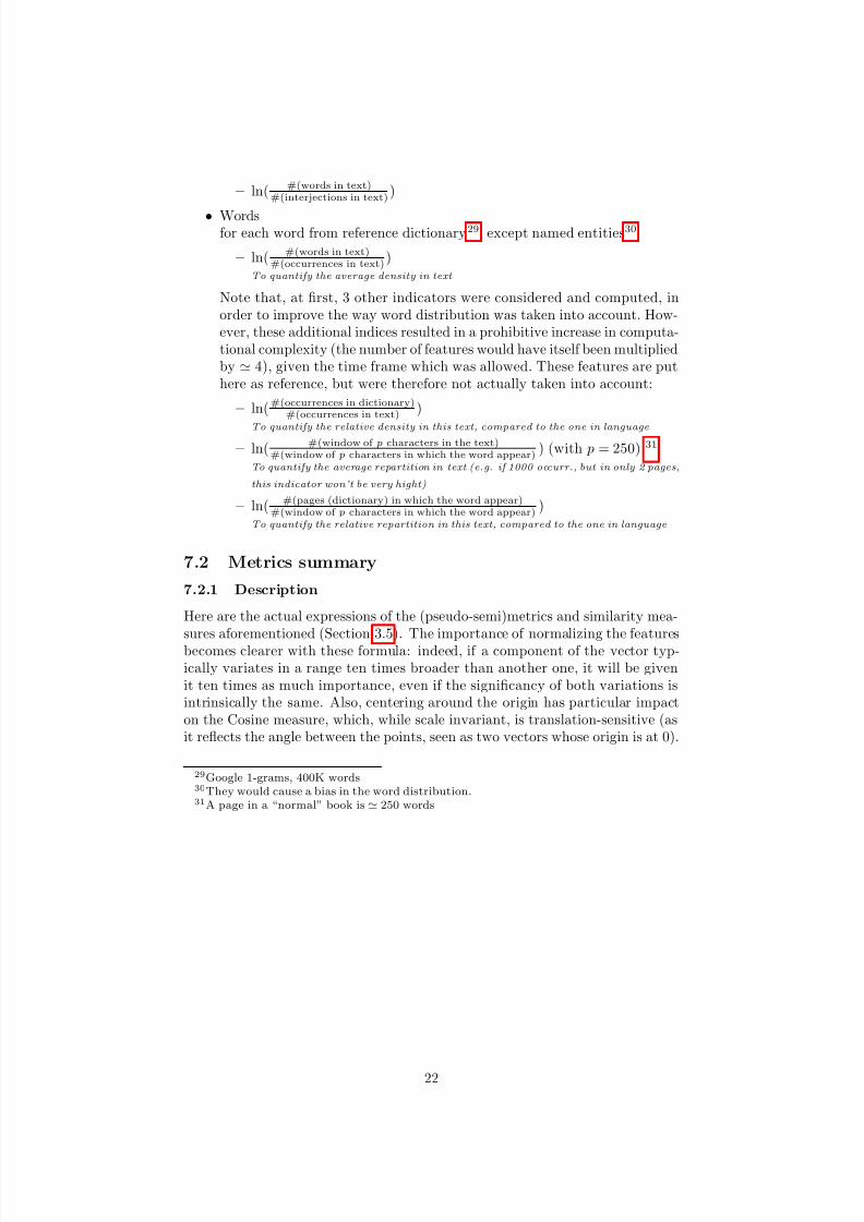
• Wordsfor each word from reference dictionary29, except named entities30

– ln( #(words in text)#(occurrences in text)

)To quantify the average density in text

Note that, at first, 3 other indicators were considered and computed, inorder to improve the way word distribution was taken into account. How-ever, these additional indices resulted in a prohibitive increase in computa-tional complexity (the number of features would have itself been multipliedby 4), given the time frame which was allowed. These features are puthere as reference, but were therefore not actually taken into account:

– ln( #(occurrences in dictionary)#(occurrences in text) )

To quantify the relative density in this text, compared to the one in language

– ln( #(window of p characters in the text)#(window of p characters in which the word appear)

) (with p = 250) 31

To quantify the average repartition in text (e.g. if 1000 occurr., but in only 2 pages,

this indicator won’t be very hight)

– ln( #(pages (dictionary) in which the word appear)#(window of p characters in which the word appear)

)To quantify the relative repartition in this text, compared to the one in language

7.2 Metrics summary

7.2.1 Description

Here are the actual expressions of the (pseudo-semi)metrics and similarity mea-sures aforementioned (Section 3.5). The importance of normalizing the featuresbecomes clearer with these formula: indeed, if a component of the vector typ-ically variates in a range ten times broader than another one, it will be givenit ten times as much importance, even if the significancy of both variations isintrinsically the same. Also, centering around the origin has particular impacton the Cosine measure, which, while scale invariant, is translation-sensitive (asit reflects the angle between the points, seen as two vectors whose origin is at 0).

29Google 1-grams, 400K words30They would cause a bias in the word distribution.31A page in a “normal” book is 250 words

22



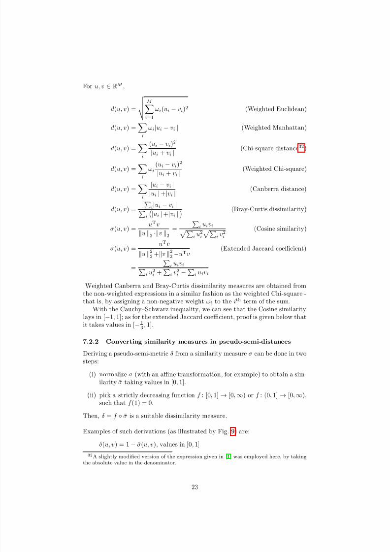
For u, v ∈ RM ,

d(u, v) =

M i=1

ωi(ui − vi)2 (Weighted Euclidean)

d(u, v) =i

ωi|ui − vi | (Weighted Manhattan)

d(u, v) =i

(ui − vi)2

|ui + vi |(Chi-square distance32)

d(u, v) =i

ωi

(ui − vi)2

|ui + vi |(Weighted Chi-square)

d(u, v) = i

|ui − vi |

|ui |+|vi |(Canberra distance)

d(u, v) =

i|ui − vi |

i

|ui |+|vi |

(Bray-Curtis dissimilarity)

σ(u, v) =uTv

u 2 ·v 2

=

i uivi

i u2i

i v2

i

(Cosine similarity)

σ(u, v) =uTv

u 22 +v 2

2 −uTv(Extended Jaccard coefficient)

=

i uivi

i u2i +

i v2

i −

i uivi

Weighted Canberra and Bray-Curtis dissimilarity measures are obtained fromthe non-weighted expressions in a similar fashion as the weighted Chi-square -that is, by assigning a non-negative weight ωi to the ith term of the sum.

With the Cauchy–Schwarz inequality, we can see that the Cosine similaritylays in [−1, 1]; as for the extended Jaccard coefficient, proof is given below thatit takes values in [−1

3, 1].

7.2.2 Converting similarity measures in pseudo-semi-distances

Deriving a pseudo-semi-metric δ from a similarity measure σ can be done in twosteps:

(i) normalize σ (with an affine transformation, for example) to obtain a sim-ilarity σ taking values in [0, 1].

(ii) pick a strictly decreasing function f : [0, 1] → [0,∞) or f : (0, 1] → [0,∞),such that f (1) = 0.

Then, δ = f ◦ σ is a suitable dissimilarity measure.

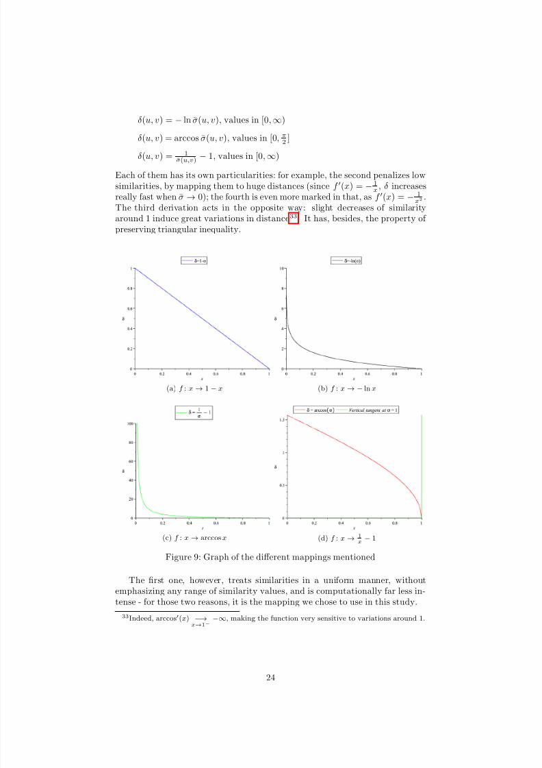
Examples of such derivations (as illustrated by Fig. 9) are:

δ(u, v) = 1− σ(u, v), values in [0, 1]

32A slightly modified version of the expression given in [1] was employed here, by takingthe absolute value in the denominator.

23



δ(u, v) = − ln σ(u, v), values in [0,∞)

δ(u, v) = arccos σ(u, v), values in [0, π2 ]

δ(u, v) = 1σ(u,v) − 1, values in [0,∞)

Each of them has its own particularities: for example, the second penalizes lowsimilarities, by mapping them to huge distances (since f (x) = − 1

x, δ increases

really fast when σ → 0); the fourth is even more marked in that, as f (x) = − 1x2

.The third derivation acts in the opposite way: slight decreases of similarityaround 1 induce great variations in distance33. It has, besides, the property of preserving triangular inequality.

(a) f : x → 1 − x (b) f : x → − ln x

(c) f : x → arccos x (d) f : x →1

x − 1

Figure 9: Graph of the different mappings mentioned

The first one, however, treats similarities in a uniform manner, withoutemphasizing any range of similarity values, and is computationally far less in-tense - for those two reasons, it is the mapping we chose to use in this study.

33Indeed, arccos(x) −→x→1−

−∞, making the function very sensitive to variations around 1.

24



7.2.3 About the Extended Jaccard index

Here can be found the proof that the Extended Jaccard coefficient (Tanimotocoefficient) takes values in [−1

3, 1]. This result was used when renormalizing it,

to derive a dissimilarity measure (cf. Appendix 7.2.2).For x, y ∈ R

n arbitrary, non both zero34, recalling that xTy = 14

x +

y 2 −x − y 2 ,σ(x, y) =

xTy

x 2 +y 2 −xTy=

xTy

x − y 2 +xTy

=1

4

x + y 2 −x − y 2

x − y 2+ 1

4

x + y 2 −x − y 2

=

x + y 2 −x − y 2

x + y 2 +3x − y 2 =

a − b

a + 3b

where a = x + y 2 and b = x− y 2, both non-negative.

(i) Since x = y if, and only if, b = 0, x = y ⇒ σ(x, y) = 1. Reciprocally,σ(x, y) = 1 ⇔ a − b = a + 3b ⇔ b = 0 ⇔ x = y, and finally

x = y ⇔ σ(x, y) = 1

(ii) Suppose x = y. Then,

σ(x, y) =ab− 1

ab

+ 3

The function ϕ : u ∈ R+ → u−1u+3 ∈ R is smooth, and ϕ(u) = 4(u+3)2 > 0,

u ∈ R+. ϕ is thus strictly increasing, meaning:

inf R+

ϕ = ϕ(0) = −1

3

supR+

ϕ = lim+∞

ϕ = 1

that is, σ(x, y) ∈ [−13

, 1), x = y; and the minimum is attained for (andonly for) a

b= 0, i.e. a = 0 or, in other terms, x = −y.

Conclusion:

∀x, y ∈ Rn, σ(x, y) ∈ [−1

3 , 1]

and σ(x, y) = 1 ⇔ x = y, while σ(x, y) = −13 ⇔ x = −y.

Miscellaneous

The programs and scripts used for this projected were developped in Python(preprocessing of the text samples), Java (for the feature extraction part, inte-grating the Stanford NLP Tools), C++ (clustering) and Matlab (result analysis).

34If x = y = 0Rn , by convention, the Extended Jaccard coefficient is equal to 1 (bothnumerator and denominator are zero).

25



References

[1] V. R. Khapli and A.S. Bhalchandra. Comparison of Similarity Metrics forThumbnail Based Image Retrieval. Journal of Computer Science and Engi-neering , 5(1):15–20, 2011. 23

[2] S.Y. Kung. Kernel-Based Machine Learning . 2011 (To be published). 5

[3] G. N. Lance and W. T. Williams. Computer programs for hierarchical poly-thetic classification (‘similarity analyses’). 9(1):60–64, May 1966. 8

[4] G. N. Lance and W. T. Williams. Mixed-Data Classificatory Programs I -Agglomerative Systems. Australian Computer Journal , 1(1):15–20, 1967. 8

[5] Christopher D. Manning, Prabhakar Raghavan, and Hinrich Schtze. Intro-

duction to Information Retrieval . Cambridge University Press, New York,NY, USA, 2008. 6

[6] Christopher D. Manning and Hinrich Schutze. Foundations of statistical natural language processing . MIT Press, 2001.

[7] Marina Meila. Comparing clusterings. 2002. 9

[8] M. Steyvers. Multidimensional Scaling. Encyclopedia of Cognitive Science,pages 1–5, 2002. 12

26

Documents

IW, Princeton, Paper