IZA DP No. 720

Labour Market Regulation, Productivity-Improving R&D and Endogenous Growth

Tapio Palokangas

February 2003

DI

SC

US

SI

ON

PA

PE

R S

ER

IE

S

Forschungsinstitutzur Zukunft der ArbeitInstitute for the Studyof Labor

Labour Market Regulation,

Productivity-Improving R&D and Endogenous Growth

Tapio Palokangas University of Helsinki

and IZA Bonn

Discussion Paper No. 720 February 2003

IZA

P.O. Box 7240 D-53072 Bonn

Germany

Tel.: +49-228-3894-0 Fax: +49-228-3894-210

Email: iza@iza.org

This Discussion Paper is issued within the framework of IZA’s research area Welfare State and Labor Market. Any opinions expressed here are those of the author(s) and not those of the institute. Research disseminated by IZA may include views on policy, but the institute itself takes no institutional policy positions. The Institute for the Study of Labor (IZA) in Bonn is a local and virtual international research center and a place of communication between science, politics and business. IZA is an independent, nonprofit limited liability company (Gesellschaft mit beschränkter Haftung) supported by the Deutsche Post AG. The center is associated with the University of Bonn and offers a stimulating research environment through its research networks, research support, and visitors and doctoral programs. IZA engages in (i) original and internationally competitive research in all fields of labor economics, (ii) development of policy concepts, and (iii) dissemination of research results and concepts to the interested public. The current research program deals with (1) mobility and flexibility of labor, (2) internationalization of labor markets, (3) welfare state and labor market, (4) labor markets in transition countries, (5) the future of labor, (6) evaluation of labor market policies and projects and (7) general labor economics. IZA Discussion Papers often represent preliminary work and are circulated to encourage discussion. Citation of such a paper should account for its provisional character. A revised version may be available on the IZA website (www.iza.org) or directly from the author.

IZA Discussion Paper No. 720 February 2003

ABSTRACT

Labour Market Regulation, Productivity-Improving R&D and Endogenous Growth

We present a growth model in which R&D increases productivity, union-firm bargaining determines the distribution of rents and the government can support unions by labour market regulation. We show that if unions are initially very strong, regulation increases only the workers’ profit share and has no impact on employment and growth. Otherwise, regulation increases wages. Because firms try to escape this cost increase through the improvement of productivity by R&D, the economy grows faster. Regulation (deregulation) is desirable when the growth rate is below (above) some critical level. JEL Classification: O40, J50 Keywords: endogenous growth, labour unions, regulation Tapio Palokangas Department of Economics University of Helsinki P.O. Box 54 00014 Helsinki Finland Tel.: +358 9 1912 4891 Fax: +358 9 1912 4877 Email: Tapio.Palokangas@helsinki.fi

1 Introduction

The problem of high unemployment and low growth, a phenomenon called

’Eurosclerosis’, is one of the most pressing economic problems in the Euro-

pean Union. Recently, the OECD Jobs Study took a stand on this problem

by arguing that strengthening competitive forces in the economy would foster

economic growth and reduce unemployment.1 To examine this, I establish

an endogenous-growth model in which unemployment is caused by efficiency

wages and union-firm bargaining. Following Blanchard and Giavazzi (2001),

we think of labour market regulation (deregulation) as increasing (decreas-

ing) the bargaining power of the labour unions.

The review of the literature shows that the relationship between growth

and labour market regulation can be highly institution-specific. Peretto

(2000) examines the effects of regulation by a product-variety model in which

labour is employed only in production and final goods can be directly used

in R&D. He also assumes that unions completely ignore that the increase

of their wages affects productivity through R&D. Peretto’s main assertion

is that a fall in union power promotes R&D and growth through a higher

profit margin. In contrast, we assume that labour is used both in production

and R&D and unions take into account also the effects through R&D.

Palokangas (1996, 2000) introduces wage bargaining into Romer’s (1990)

product-variety model in which R&D employs labour only but final goods

are produced from skilled labour, unskilled labour and intermediate prod-

ucts. He shows that higher relative union bargaining power leads to a higher

growth rate as follows. Because R&D employs skilled labour and increases

aggregate labour income, the union does not accept any agreement causing

unemployment of skilled labour. With full employment of skilled labour, the

increase in union power speeds up economic growth through a transfer of

skilled labour from the production of final goods to R&D. This conclusion

results however from three specific assumptions. First, bargaining is carried

out at the level of an industry or the economy rather than at the level of

a single firm. Second, there are two separate labour inputs, skilled and un-

1Cf. OECD (1994), pp. 23 and 53: ’Establishing a competitive environment could,therefore, improve job prospects by both eliminating wage premia and encouraging outputexpansion.’

1

skilled labour, which are both organized in the same labour union. Third,

there are no efficiency wages. In contrast, we assume union-firm bargaining,

homogeneous labour and efficiency wages.

This paper is organized as follows. Labour market imperfections, which

play a crucial role in the analysis, are presented in section 2. Sections 3 and 4

specify the behaviour of consumers and high-tech firms. Section 5 considers

union-firm bargaining and section 6 optimal labour market regulation.

2 The labour market

The economy consists of two sectors that produce consumption goods. The

high-tech sector contains a fixed number n of similar price-setting firms (in-

dexed i = 1, ..., n), each of which manufactures one variety of the differen-

tiated products, produces new knowledge and uses labour, knowledge and

some non-traded factor as inputs. The traditional sector comprises competi-

tive firms that produce unit of output from one labour unit. A high-tech firm

and a firm-specific union bargain over the wage and the workers’ profit share

taking macroeconomic variables (e.g. the price level, aggregate consumption,

the expected labour income elsewhere) as given. Labour market regulation

determines relative union bargaining power.

We assume that labour supply N is fixed, for simplicity. Because the

traditional sector is competitive, we obtain the equilibrium condition

L +n∑

i=1

li = N, (1)

where L is the employment of physical labour in the traditional sector and

li is that in the ith high-tech firm (hereafter firm i). Firm i pays a share si

of its profit πi to its workers in proportion to employment. Since the profit

share is non-negative for both parties, we obtain

0 ≤ si ≤ 1. (2)

The total wage is then given by

vi.= wi + siπi/li, (3)

2

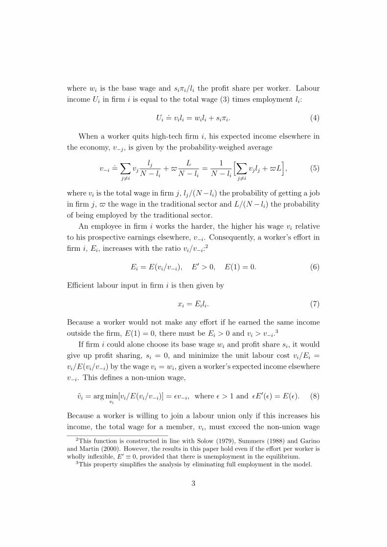
where wi is the base wage and siπi/li the profit share per worker. Labour

income Ui in firm i is equal to the total wage (3) times employment li:

Ui.= vili = wili + siπi. (4)

When a worker quits high-tech firm i, his expected income elsewhere in

the economy, v−j, is given by the probability-weighed average

v−i.=

∑j 6=i

vjlj

N − li+ $

L

N − li=

1

N − li

[∑j 6=i

vjlj + $L], (5)

where vi is the total wage in firm j, lj/(N−li) the probability of getting a job

in firm j, $ the wage in the traditional sector and L/(N − li) the probability

of being employed by the traditional sector.

An employee in firm i works the harder, the higher his wage vi relative

to his prospective earnings elsewhere, v−i. Consequently, a worker’s effort in

firm i, Ei, increases with the ratio vi/v−i:2

Ei = E(vi/v−i), E ′ > 0, E(1) = 0. (6)

Efficient labour input in firm i is then given by

xi = Eili. (7)

Because a worker would not make any effort if he earned the same income

outside the firm, E(1) = 0, there must be Ei > 0 and vi > v−i.3

If firm i could alone choose its base wage wi and profit share si, it would

give up profit sharing, si = 0, and minimize the unit labour cost vi/Ei =

vi/E(vi/v−i) by the wage vi = wi, given a worker’s expected income elsewhere

v−i. This defines a non-union wage,

vi = arg minvi

[vi/E(vi/v−i)] = εv−i, where ε > 1 and εE ′(ε) = E(ε). (8)

Because a worker is willing to join a labour union only if this increases his

income, the total wage for a member, vi, must exceed the non-union wage

2This function is constructed in line with Solow (1979), Summers (1988) and Garinoand Martin (2000). However, the results in this paper hold even if the effort per worker iswholly inflexible, E′ ≡ 0, provided that there is unemployment in the equilibrium.

3This property simplifies the analysis by eliminating full employment in the model.

3

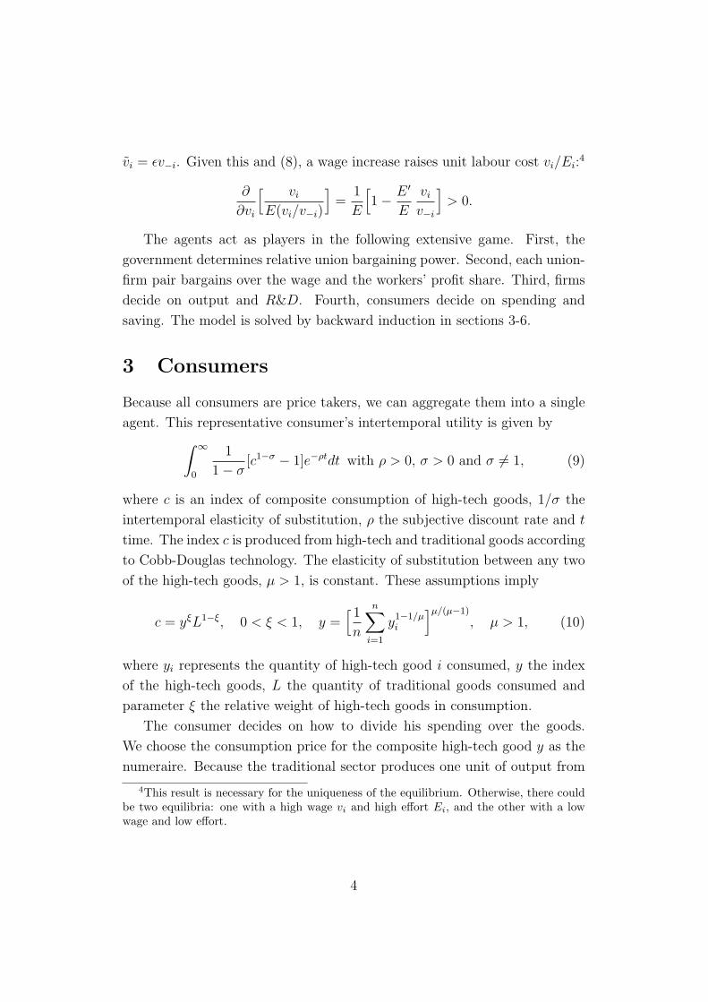
vi = εv−i. Given this and (8), a wage increase raises unit labour cost vi/Ei:4

∂

∂vi

[ vi

E(vi/v−i)

]=

1

E

[1− E ′

E

vi

v−i

]> 0.

The agents act as players in the following extensive game. First, the

government determines relative union bargaining power. Second, each union-

firm pair bargains over the wage and the workers’ profit share. Third, firms

decide on output and R&D. Fourth, consumers decide on spending and

saving. The model is solved by backward induction in sections 3-6.

3 Consumers

Because all consumers are price takers, we can aggregate them into a single

agent. This representative consumer’s intertemporal utility is given by∫ ∞

0

1

1− σ[c1−σ − 1]e−ρtdt with ρ > 0, σ > 0 and σ 6= 1, (9)

where c is an index of composite consumption of high-tech goods, 1/σ the

intertemporal elasticity of substitution, ρ the subjective discount rate and t

time. The index c is produced from high-tech and traditional goods according

to Cobb-Douglas technology. The elasticity of substitution between any two

of the high-tech goods, µ > 1, is constant. These assumptions imply

c = yξL1−ξ, 0 < ξ < 1, y =[ 1

n

n∑i=1

y1−1/µi

]µ/(µ−1)

, µ > 1, (10)

where yi represents the quantity of high-tech good i consumed, y the index

of the high-tech goods, L the quantity of traditional goods consumed and

parameter ξ the relative weight of high-tech goods in consumption.

The consumer decides on how to divide his spending over the goods.

We choose the consumption price for the composite high-tech good y as the

numeraire. Because the traditional sector produces one unit of output from

4This result is necessary for the uniqueness of the equilibrium. Otherwise, there couldbe two equilibria: one with a high wage vi and high effort Ei, and the other with a lowwage and low effort.

4

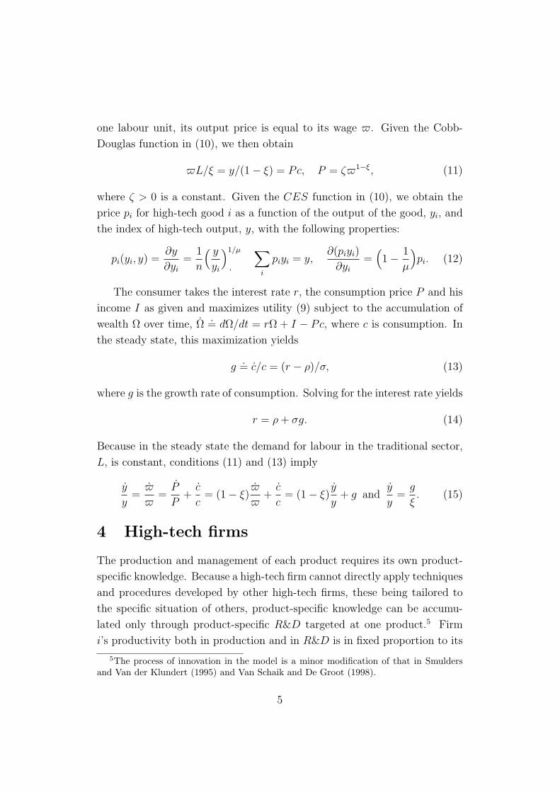
one labour unit, its output price is equal to its wage $. Given the Cobb-

Douglas function in (10), we then obtain

$L/ξ = y/(1− ξ) = Pc, P = ζ$1−ξ, (11)

where ζ > 0 is a constant. Given the CES function in (10), we obtain the

price pi for high-tech good i as a function of the output of the good, yi, and

the index of high-tech output, y, with the following properties:

pi(yi, y) =∂y

∂yi

=1

n

( y

yi

)1/µ

,

∑i

piyi = y,∂(piyi)

∂yi

=(1− 1

µ

)pi. (12)

The consumer takes the interest rate r, the consumption price P and his

income I as given and maximizes utility (9) subject to the accumulation of

wealth Ω over time, Ω.= dΩ/dt = rΩ + I − Pc, where c is consumption. In

the steady state, this maximization yields

g.= c/c = (r − ρ)/σ, (13)

where g is the growth rate of consumption. Solving for the interest rate yields

r = ρ + σg. (14)

Because in the steady state the demand for labour in the traditional sector,

L, is constant, conditions (11) and (13) imply

y

y=

$

$=

P

P+

c

c= (1− ξ)

$

$+

c

c= (1− ξ)

y

y+ g and

y

y=

g

ξ. (15)

4 High-tech firms

The production and management of each product requires its own product-

specific knowledge. Because a high-tech firm cannot directly apply techniques

and procedures developed by other high-tech firms, these being tailored to

the specific situation of others, product-specific knowledge can be accumu-

lated only through product-specific R&D targeted at one product.5 Firm

i’s productivity both in production and in R&D is in fixed proportion to its

5The process of innovation in the model is a minor modification of that in Smuldersand Van der Klundert (1995) and Van Schaik and De Groot (1998).

5

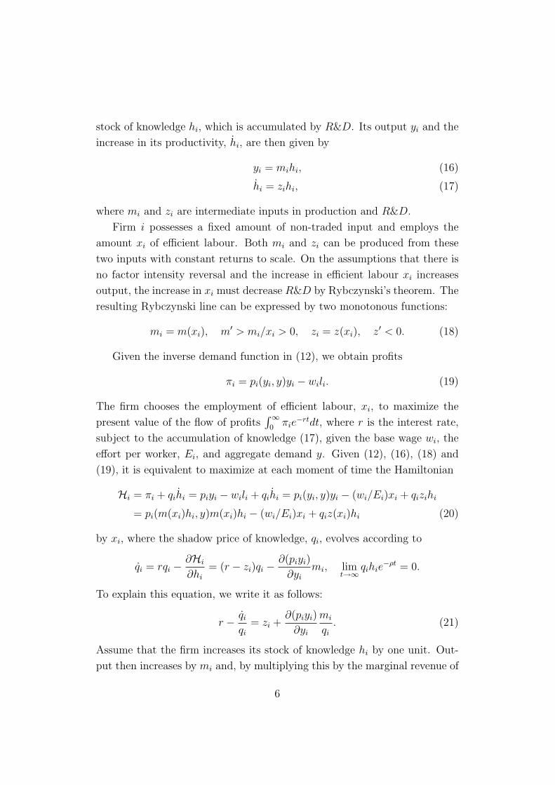
stock of knowledge hi, which is accumulated by R&D. Its output yi and the

increase in its productivity, hi, are then given by

yi = mihi, (16)

hi = zihi, (17)

where mi and zi are intermediate inputs in production and R&D.

Firm i possesses a fixed amount of non-traded input and employs the

amount xi of efficient labour. Both mi and zi can be produced from these

two inputs with constant returns to scale. On the assumptions that there is

no factor intensity reversal and the increase in efficient labour xi increases

output, the increase in xi must decrease R&D by Rybczynski’s theorem. The

resulting Rybczynski line can be expressed by two monotonous functions:

mi = m(xi), m′ > mi/xi > 0, zi = z(xi), z′ < 0. (18)

Given the inverse demand function in (12), we obtain profits

πi = pi(yi, y)yi − wili. (19)

The firm chooses the employment of efficient labour, xi, to maximize the

present value of the flow of profits∫∞

0πie

−rtdt, where r is the interest rate,

subject to the accumulation of knowledge (17), given the base wage wi, the

effort per worker, Ei, and aggregate demand y. Given (12), (16), (18) and

(19), it is equivalent to maximize at each moment of time the Hamiltonian

Hi = πi + qihi = piyi − wili + qihi = pi(yi, y)yi − (wi/Ei)xi + qizihi

= pi(m(xi)hi, y)m(xi)hi − (wi/Ei)xi + qiz(xi)hi (20)

by xi, where the shadow price of knowledge, qi, evolves according to

qi = rqi −∂Hi

∂hi

= (r − zi)qi −∂(piyi)

∂yi

mi, limt→∞

qihie−ρt = 0.

To explain this equation, we write it as follows:

r − qi

qi

= zi +∂(piyi)

∂yi

mi

qi

. (21)

Assume that the firm increases its stock of knowledge hi by one unit. Out-

put then increases by mi and, by multiplying this by the marginal revenue of

6

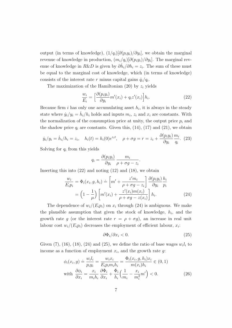
output (in terms of knowledge), (1/qi)[∂(piyi)/∂yi], we obtain the marginal

revenue of knowledge in production, (mi/qi)[∂(piyi)/∂yi]. The marginal rev-

enue of knowledge in R&D is given by ∂hi/∂hi = zi. The sum of these must

be equal to the marginal cost of knowledge, which (in terms of knowledge)

consists of the interest rate r minus capital gains qi/qi.

The maximization of the Hamiltonian (20) by zi yields

wi

Ei

=[∂(piyi)

∂yi

m′(xi) + qiz′(xi)

]hi. (22)

Because firm i has only one accumulating asset hi, it is always in the steady

state where yi/yi = hi/hi holds and inputs mi, zi and xi are constants. With

the normalization of the consumption price at unity, the output price pi and

the shadow price qi are constants. Given this, (14), (17) and (21), we obtain

yi/yi = hi/hi = zi, hi(t) = hi(0)ezit, ρ + σg = r = zi +

∂(piyi)

∂yi

mi

qi

. (23)

Solving for qi from this yields

qi =∂(piyi)

∂yi

mi

ρ + σg − zi

.

Inserting this into (22) and noting (12) and (18), we obtain

wi

Eipi

= Φi(xi, g, hi).=

[m′ +

z′mi

ρ + σg − zi

]∂(piyi)

∂yi

hi

pi

=(1− 1

µ

) [m′(xi) +

z′(xi)m(xi)

ρ + σg − z(xi)

]hi. (24)

The dependence of wi/(Eipi) on xi through (24) is ambiguous. We make

the plausible assumption that given the stock of knowledge, hi, and the

growth rate g (or the interest rate r = ρ + σg), an increase in real unit

labour cost wi/(Eipi) decreases the employment of efficient labour, xi:

∂Φi/∂xi < 0. (25)

Given (7), (16), (18), (24) and (25), we define the ratio of base wages wili to

income as a function of employment xi, and the growth rate g:

φi(xi, g).=

wilipiyi

=wixi

Eipimihi

=Φi(xi, g, hi)xi

m(xi)hi

∈ (0, 1)

with∂φi

∂xi

=xi

mihi

∂Φi

∂xi

+Φi

hi

( 1

mi

− xi

m2i

m′)

< 0. (26)

7

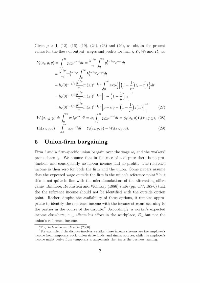
Given µ > 1, (12), (16), (19), (24), (23) and (26), we obtain the present

values for the flows of output, wages and profits for firm i, Yi, Wi and Pi, as:

Yi(xi, g, y).=

∫ ∞

0

piyie−rtdt =

y1/µ

n

∫ ∞

0

y1−1/µi e−rtdt

=y1/µ

nm

1−1/µi

∫ ∞

0

h1−1/µi e−rtdt

= hi(0)1−1/µ y1/µ

nm(xi)

1−1/µ

∫ ∞

0

exp[(

1− 1

µ

)zi − r

]t

dt

= hi(0)1−1/µ y1/µ

nm(xi)

1−1/µ[r −

(1− 1

µ

)zi

]−1

= hi(0)1−1/µ y1/µ

nm(xi)

1−1/µ[ρ + σg −

(1− 1

µ

)z(xi)

]−1

,(27)

Wi(xi, g, y).=

∫ ∞

0

wilie−rtdt = φi

∫ ∞

0

piyie−rtdt = φi(xi, g)Yi(xi, g, y), (28)

Πi(xi, g, y).=

∫ ∞

0

πie−rtdt = Yi(xi, g, y)−Wi(xi, g, y). (29)

5 Union-firm bargaining

Firm i and a firm-specific union bargain over the wage wi and the workers’

profit share si. We assume that in the case of a dispute there is no pro-

duction, and consequently no labour income and no profits. The reference

income is then zero for both the firm and the union. Some papers assume

that the expected wage outside the firm is the union’s reference point,6 but

this is not quite in line with the microfoundations of the alternating offers

game. Binmore, Rubinstein and Wolinsky (1986) state (pp. 177, 185-6) that

the the reference income should not be identified with the outside option

point. Rather, despite the availability of these options, it remains appro-

priate to identify the reference income with the income streams accruing to

the parties in the course of the dispute.7 Accordingly, a worker’s expected

income elsewhere, v−i, affects his effort in the workplace, Ei, but not the

union’s reference income.

6E.g. in Garino and Martin (2000).7For example, if the dispute involves a strike, these income streams are the employee’s

income from temporary work, union strike funds, and similar sources, while the employer’sincome might derive from temporary arrangements that keeps the business running.

8

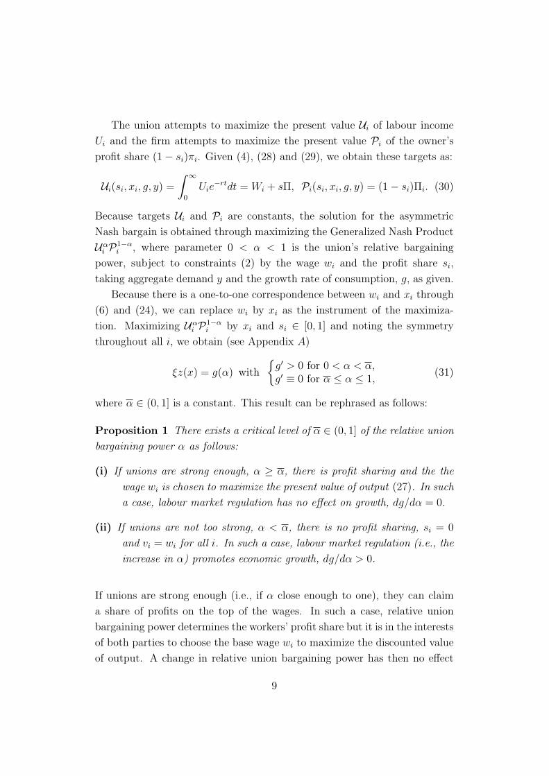
The union attempts to maximize the present value Ui of labour income

Ui and the firm attempts to maximize the present value Pi of the owner’s

profit share (1− si)πi. Given (4), (28) and (29), we obtain these targets as:

Ui(si, xi, g, y) =

∫ ∞

0

Uie−rtdt = Wi + sΠ, Pi(si, xi, g, y) = (1− si)Πi. (30)

Because targets Ui and Pi are constants, the solution for the asymmetric

Nash bargain is obtained through maximizing the Generalized Nash Product

Uαi P1−α

i , where parameter 0 < α < 1 is the union’s relative bargaining

power, subject to constraints (2) by the wage wi and the profit share si,

taking aggregate demand y and the growth rate of consumption, g, as given.

Because there is a one-to-one correspondence between wi and xi through

(6) and (24), we can replace wi by xi as the instrument of the maximiza-

tion. Maximizing Uαi P1−α

i by xi and si ∈ [0, 1] and noting the symmetry

throughout all i, we obtain (see Appendix A)

ξz(x) = g(α) with

g′ > 0 for 0 < α < α,g′ ≡ 0 for α ≤ α ≤ 1,

(31)

where α ∈ (0, 1] is a constant. This result can be rephrased as follows:

Proposition 1 There exists a critical level of α ∈ (0, 1] of the relative union

bargaining power α as follows:

(i) If unions are strong enough, α ≥ α, there is profit sharing and the the

wage wi is chosen to maximize the present value of output (27). In such

a case, labour market regulation has no effect on growth, dg/dα = 0.

(ii) If unions are not too strong, α < α, there is no profit sharing, si = 0

and vi = wi for all i. In such a case, labour market regulation (i.e., the

increase in α) promotes economic growth, dg/dα > 0.

If unions are strong enough (i.e., if α close enough to one), they can claim

a share of profits on the top of the wages. In such a case, relative union

bargaining power determines the workers’ profit share but it is in the interests

of both parties to choose the base wage wi to maximize the discounted value

of output. A change in relative union bargaining power has then no effect

9

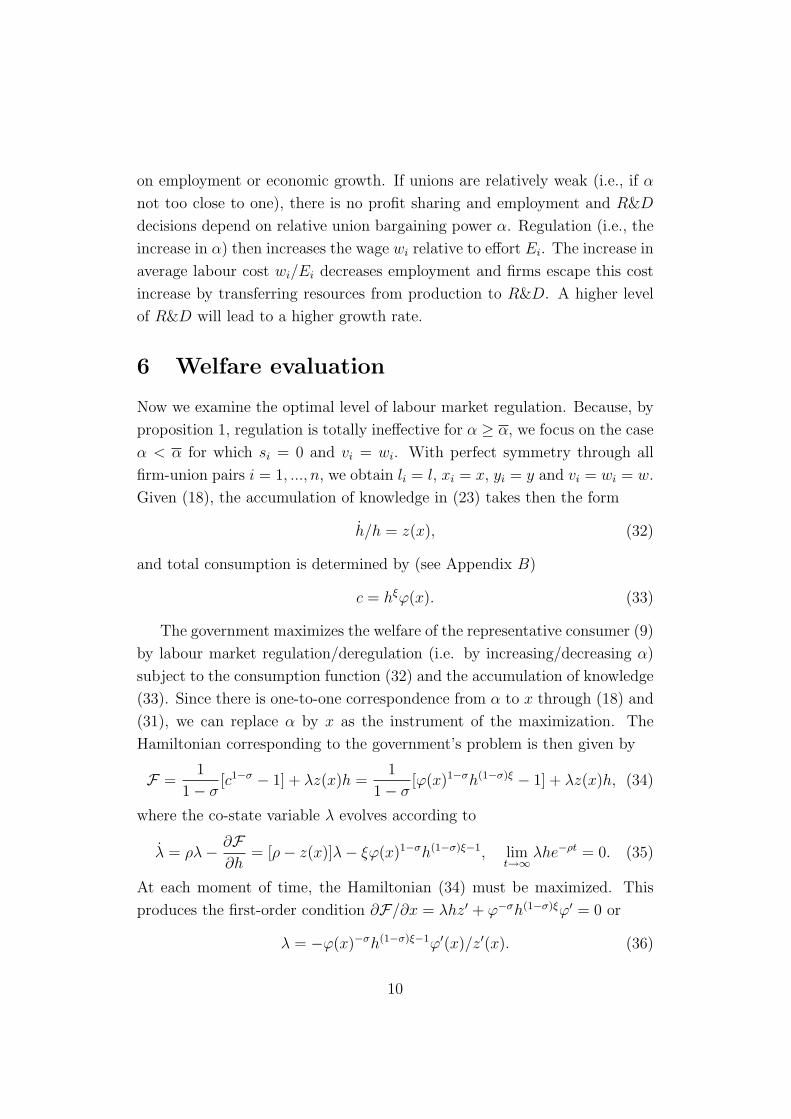
on employment or economic growth. If unions are relatively weak (i.e., if α

not too close to one), there is no profit sharing and employment and R&D

decisions depend on relative union bargaining power α. Regulation (i.e., the

increase in α) then increases the wage wi relative to effort Ei. The increase in

average labour cost wi/Ei decreases employment and firms escape this cost

increase by transferring resources from production to R&D. A higher level

of R&D will lead to a higher growth rate.

6 Welfare evaluation

Now we examine the optimal level of labour market regulation. Because, by

proposition 1, regulation is totally ineffective for α ≥ α, we focus on the case

α < α for which si = 0 and vi = wi. With perfect symmetry through all

firm-union pairs i = 1, ..., n, we obtain li = l, xi = x, yi = y and vi = wi = w.

Given (18), the accumulation of knowledge in (23) takes then the form

h/h = z(x), (32)

and total consumption is determined by (see Appendix B)

c = hξϕ(x). (33)

The government maximizes the welfare of the representative consumer (9)

by labour market regulation/deregulation (i.e. by increasing/decreasing α)

subject to the consumption function (32) and the accumulation of knowledge

(33). Since there is one-to-one correspondence from α to x through (18) and

(31), we can replace α by x as the instrument of the maximization. The

Hamiltonian corresponding to the government’s problem is then given by

F =1

1− σ[c1−σ − 1] + λz(x)h =

1

1− σ[ϕ(x)1−σh(1−σ)ξ − 1] + λz(x)h, (34)

where the co-state variable λ evolves according to

λ = ρλ− ∂F∂h

= [ρ− z(x)]λ− ξϕ(x)1−σh(1−σ)ξ−1, limt→∞

λhe−ρt = 0. (35)

At each moment of time, the Hamiltonian (34) must be maximized. This

produces the first-order condition ∂F/∂x = λhz′ + ϕ−σh(1−σ)ξϕ′ = 0 or

λ = −ϕ(x)−σh(1−σ)ξ−1ϕ′(x)/z′(x). (36)

10

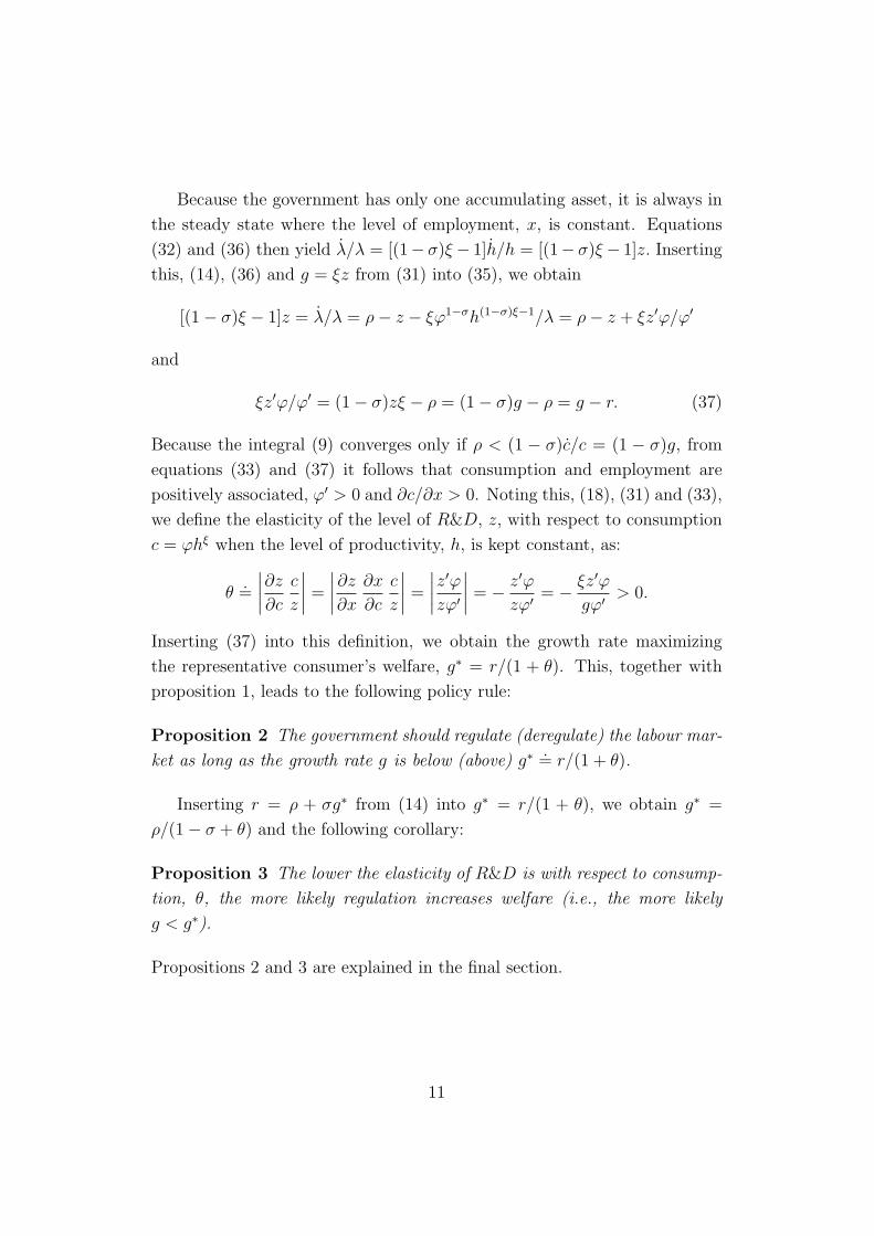
Because the government has only one accumulating asset, it is always in

the steady state where the level of employment, x, is constant. Equations

(32) and (36) then yield λ/λ = [(1− σ)ξ− 1]h/h = [(1− σ)ξ− 1]z. Inserting

this, (14), (36) and g = ξz from (31) into (35), we obtain

[(1− σ)ξ − 1]z = λ/λ = ρ− z − ξϕ1−σh(1−σ)ξ−1/λ = ρ− z + ξz′ϕ/ϕ′

and

ξz′ϕ/ϕ′ = (1− σ)zξ − ρ = (1− σ)g − ρ = g − r. (37)

Because the integral (9) converges only if ρ < (1 − σ)c/c = (1 − σ)g, from

equations (33) and (37) it follows that consumption and employment are

positively associated, ϕ′ > 0 and ∂c/∂x > 0. Noting this, (18), (31) and (33),

we define the elasticity of the level of R&D, z, with respect to consumption

c = ϕhξ when the level of productivity, h, is kept constant, as:

θ.=

∣∣∣∣∂z

∂c

c

z

∣∣∣∣ =

∣∣∣∣∂z

∂x

∂x

∂c

c

z

∣∣∣∣ =

∣∣∣∣z′ϕzϕ′

∣∣∣∣ = − z′ϕ

zϕ′= − ξz′ϕ

gϕ′> 0.

Inserting (37) into this definition, we obtain the growth rate maximizing

the representative consumer’s welfare, g∗ = r/(1 + θ). This, together with

proposition 1, leads to the following policy rule:

Proposition 2 The government should regulate (deregulate) the labour mar-

ket as long as the growth rate g is below (above) g∗.= r/(1 + θ).

Inserting r = ρ + σg∗ from (14) into g∗ = r/(1 + θ), we obtain g∗ =

ρ/(1− σ + θ) and the following corollary:

Proposition 3 The lower the elasticity of R&D is with respect to consump-

tion, θ, the more likely regulation increases welfare (i.e., the more likely

g < g∗).

Propositions 2 and 3 are explained in the final section.

11

7 Conclusions

In this paper, efficiency wages, union-firm bargaining and profit sharing were

incorporated into a unified framework of endogenous growth. We were inter-

ested in how regulation (deregulation), which strengthens (weakens) unions

in bargaining, affects economic growth. An employee works the harder, the

more more the wage in the firm exceeds the expected labour income outside

the firm. A firm accumulates knowledge and increases its productivity by

doing R&D. In this framework, we obtain the following results.

Provided that union power is not initially too high, labour market regu-

lation decreases employment and current consumption but fosters economic

growth. When union bargaining position is improved, wages increase rela-

tive to a worker’s effort and firms try to escape this cost increase through

improved productivity, by increasing its R&D. With larger R&D, the econ-

omy will grow at a faster rate. If unions are strong enough, they can claim

a share of profits on the top of their wages. Unions and firms then share the

profit in fixed proportion to their relative bargaining power and maximize

the discounted value of total income by the wage, so that labour market

regulation will not affect R&D and growth.

The desirability of regulation or deregulation depends on whether eco-

nomic growth is too fast or too slow from the welfare point of view. If this is

too fast, the labour market should be deregulated to slow down technological

change. Overly slow growth can be eliminated by labour market regulation.

The higher the elasticity of R&D with respect to consumption (given the

interest rate), the more likely regulation increases welfare. Consumption and

R&D are produced from the same resources. The more a decrease in current

consumption by one unit increases future consumption through larger R&D

and a higher growth rate, the higher is the welfare-maximizing growth rate

and the more likely actual growth should be promoted by regulation.

While a great deal of caution should be exercised when a highly stylized

mathematical model is used to draw conclusions about the effects of regula-

tion on growth, the following judgement nevertheless seems to be justified.

Since the institutional specification of the labour market is significant for the

outcome of regulation, in contrast to the OECD Jobs Study, strengthening

competitive forces in the labour market may slow down economic growth.

12

Appendix

A. The proof of result (31)

We deduce first two useful subresults. Given (27), we obtain

∂2 log Yi

∂xi∂y= 0. (38)

Because there is symmetry through all i, in the macroeconomic equilibrium

there must be zi = z, xi = x, li = l, yi = y and vi = v. Given this, (10),

(15), (18) and (23), we obtain

g = ξy

y=

ξ

y

n∑k=1

∂y

∂yk

yk =ξ

n

n∑k=1

( y

yk

)1/µ−1

zk, g∣∣yk=y

=ξ

n

n∑k=1

z(xk). (39)

Given equations (4), (12), (16) and (28)-(30), we define a function

Γi(si, xi, g, y, α).= log[Uα

i P1−αi ] = α log Ui + (1− α) log Pi

= α log[Wi(xi, g, y) + siΠi(xi, g, y)] + (1− α)[log Πi(xi, g, y) + log(1− si)]

= α log[(1− si)Wi + siYi] + (1− α) log(Yi −Wi) + (1− α) log(1− si)

= log Y (xi, g, y) + α log[(1− si)φi(xi, g) + si] + (1− α) log[1− φi(xi, g)]

+ (1− α) log(1− si). (40)

The outcome of bargaining is obtained through maximizing the logarithm of

the Nash product (40) s.t. 0 ≤ si ≤ 1 by xi and si, keeping g and y constant.

This is equivalent to the maximization of the Lagrangean

Li = Γi(si, xi, g, y, α) + χ1si + χ2(1− si)

subject to Kuhn-Tucker conditions

χ1si = 0, χ1 ≥ 0, χ2(1− si) = 0, χ2 ≥ 0. (41)

Given (40), we obtain the first-order conditions for si and xi as:

∂Li

∂si

=∂Γi

∂si

+ χ1 − χ2 =α(1− φi)

(1− si)φi + si

− 1− α

1− si

+ χ1 − χ2 = 0,

∂Li/∂xi = ∂Γi/∂xi = 0. (42)

13

Consider first the case where

either α = 1 or1− α

α=

(1− si)(1− φi)

(1− si)φi + si

. (43)

If α = 1, then (40), (41) and (42) produce

χ2 =1− φi

(1− si)φi + si

+ χ1 > χ1 ≥ 0, s = 1, Γi = log Yi.

This means that the maximization of (40) by xi is equivalent to the maxi-

mization of the present value of output, Yi, by xi:

xi = arg maxxi

Yi(xi, g, y). (44)

Next, assume α < 1 and

1− α

α=

(1− si)(1− φi)

(1− si)φi + si

. (45)

This, (29) and (40) yield (1− si)φi + si = α, (1− si)(1− φi) = 1− α and

Γi = log Yi(zi, g, y) + constants.

Again, the maximization of (40) by xi is equivalent to the maximization of Yi

by xi. We conclude that if (43) holds, then xi is determined by (44). Noting

this and the first-order condition for xi, we can define a constant

α = infα| ∂Li/∂xi = 0 and (43) holds

≤ 1. (46)

Because in the model there is symmetry through all i, this yields

xi = x = arg maxx

Yi(x, g, y) for α ≥ α. (47)

From (39) and (47) it follows that inputs xi for all i and the growth rate g

are independent of α for α ≥ α.

If α → 0, then given (41) and (42) we obtain

χ1 = (1− α)/(1− si) + χ2 > χ2 ≥ 0, si = 0.

Hence, for sufficiently small values of α condition (43) cannot hold. Given

this result and (46), there must be α > 0. Because condition (44) holds for

α ≤ α ≤ 1, the equilibrium of the system is independent of α and

dz/dα = 0 for α ≤ α ≤ 1. (48)

14

Finally, consider the case

0 < α < α. (49)

It follows that (43) does not hold and

α < 1,1− α

α6= (1− si)(1− φi)

(1− si)φi + si

. (50)

holds. Because si = 1 is in contradiction with (50), si < 1 obtains. From

si < 1, (41), (42) and (50) it follows

χ2 = 0, χ1 =1− α

1− si

− α(1− φi)

(1− si)φi + si

> 0, si = 0.

Given si = 0, the function (40) takes the form

Γi(0, xi, g, α, y) = log Y (xi, g, y) + α log φi(xi, g) + (1− α) log[1− φi(xi, g)],

and the remaining first-order condition the form

∂Γi

∂xi

=∂ log Yi(xi, g, y)

∂xi

+α/φi(xi, g)− 1

1− φi(xi, g)

∂φi(xi, g)

∂xi

= 0. (51)

This, (26) and (38) yield

∂2Γi

∂xi∂c=

∂2 log Yi

∂xi∂c= 0,

∂2Γi

∂xi∂α=

1

(1− φi)φi

∂φi

∂xi

< 0. (52)

Noting (26), (52) and the second-order condition ∂2Γi/∂x2i < 0, and differ-

entiating the first-order condition (51) totally, we define the function

xi = Ψ(α, g) with∂Ψ

∂α= − ∂2Γi

∂xi∂α

/∂2Γi

∂x2i

< 0 for 0 < α < α. (53)

Noting the symmetry over i and inserting the right-hand equation of (39)

into the functions (53), we obtain a system of n equations

∆i = xi −Ψ(α, g) = xi −Ψ(α,

ξ

n

∑k

z(xk))

= 0 for j = 1, ..., n, (54)

with endogenous variables x1, ..., xn. Differentiating the system (54), we ob-

tain the coefficient matrix (∂∆i/∂xk

)n×n .

(55)

15

The reaction function for each sector i is given by (54). With perfect symme-

try over all sectors i, the sufficient conditions for the stability of the equilib-

rium imply that the coefficient matrix (55) is subject to diagonal dominance.8

Noting the symmetry over xk for k 6= i as well as equations (54), we obtain

the diagonal dominance into the form

0 <∂∆i

∂xi

±∑k 6=i

∂∆i

∂xk

= 1− ξ

n

∂Ψ

∂gz′(xi)±

ξ

n

∑k 6=i

∂Ψ

∂gz′(xk)

= 1−[ 1

n±

(1− 1

n

)]ξ∂Ψ

∂gz′ for k 6= i.

This implies ξ z′ ∂Ψ/∂g < 1. Noting the symmetry throughout all k, we ob-

tain xk = x for all k and z(x) = g/ξ. Functions (53) can then be transformed

into Ψ(α, g) = x = z−1(g/ξ), where z−1 is the inverse function of z(x). Dif-

ferentiating this equation and noting (18) and (53) and ξ z′∂Ψ/∂g < 1, we

obtain ∂Ψ/∂g > 1/(ξ z′) and

ξz = g(α) with g′.=

dg

dα=

∂Ψ

∂α

/( 1

ξz′− ∂Ψ

∂g

)> 0 for 0 < α < α. (56)

Results (48) and (56) can be summarized as (31).

B. The proof of result (33)

Noting symmetry li = l, xi = x, zi = z, yi = y and vi = wi = w and

using equations (11), (12) and (26), we obtain

pi = 1/n, $L = ξy/(1− ξ), v = w = φiy/(nl). (57)

Given these and (18), equations (1), (5), (6), (7) and (31) take then the form

L + nl = N, l = xi/Ei = x/E(v/v−i), g = ξz,

v−i

v=

1

N − l

[(n− 1)l +

$

vL

]=

1

N − l

[(n− 1)l +

ξ

1− ξ

nl

φi(z, g)

]=

1

N/l − 1

[n− 1 +

ξ

1− ξ

n

φi(Z, ξZ)

]. (58)

In the system (58), there are four equations, four endogenous variables L,

l, g and v/v−i and one exogenous variable x. By the comparative statics of

8See, for example, Dixit (1986), p. 117. Here, the diagonal term 1 is positive, so thatthe inequality must be greater than zero.

16

this system, we can define L as a function of x. Equations (10), (16), (17)

and (18) as well as the function L(x) produce

c = yξL1−ξ = hξm(x)ξL(x)1−ξ = hξϕ(x) with ϕ(x).= m(x)ξL(x)1−ξ.

References:

Binmore, K., Rubinstein, A. and Wolinsky, A. (1986). The Nash bargaining

solution in economic modelling. Rand Journal of Economics 17, 176-188.

Blanchard, O. and Giavazzi, F. (2001). Macroeconomic effect of regulation

and deregulation in goods and labor markets. Working paper 01-02, Depart-

ment of Economics, MIT.

Dixit, A. (1986). Comparative statics for oligopoly, International Economic

Review 27. 107-122.

Garino, G. and Martin, C. (2000). Efficiency wages and union-firm bargain-

ing. Economics Letters 69, 181-185.

The OECD Jobs Study; Evidence and Explanations Part II. Paris 1994.

Palokangas, T. (1996). Endogenous growth and collective bargaining. Jour-

nal of Economic Dynamics and Control 20, 925-944.

Palokangas, T. (2000). Labour Unions, Public Policy and Economic Growth.

Cambridge (U.K.): Cambridge University Press.

Peretto, P.F. (1998). Market power, growth and unemployment. Duke Eco-

nomics Working Paper 98-16.

Romer, P.M. (1990). Endogenous technological change. Journal of Political

Economy 98, S71-S102.

Smulders, S. and Van de Klundert, T. (1995). Imperfect competition, con-

centration and growth with firm-specific R&D. European Economic Review

39, 139-160.

Solow, R. (1979). Another possible source of wage stickiness. Journal of

Macroeconomics 1, 79-82.

Summers, L.H. (1988). Relative wages, efficiency wages and keynesian un-

employment. American Economic Review 78, 383-388.

Van Schaik, A.B.M. and De Groot, H.L.F. (1998). Unemployment and en-

dogenous growth. Labour 12, 189-219.

17

IZA Discussion Papers No.

Author(s) Title

Area Date

705 G. Brunello D. Checchi

School Quality and Family Background in Italy 2 01/03

706 S. Girma H. Görg

Blessing or Curse? Domestic Plants' Survival and Employment Prospects after Foreign Acquisitions

1 01/03

707 C. Schnabel J. Wagner

Trade Union Membership in Eastern and Western Germany: Convergence or Divergence?

3 01/03

708 C. Schnabel J. Wagner

Determinants of Trade Union Membership in Western Germany: Evidence from Micro Data, 1980-2000

3 01/03

709 L. Danziger S. Neuman

Delays in Renewal of Labor Contracts: Theory and Evidence

1 02/03

710 Z. Eckstein Y. Weiss

On the Wage Growth of Immigrants: Israel, 1990-2000

2 02/03

711 C. Ruhm Healthy Living in Hard Times

3 02/03

712 E. Fehr J. Henrich

Is Strong Reciprocity a Maladaptation? On the Evolutionary Foundations of Human Altruism

5 02/03

713 I. Gang J. Landon-Lane M. S. Yun

Does the Glass Ceiling Exist? A Cross-National Perspective on Gender Income Mobility

2 02/03

714 M. Fertig Educational Production, Endogenous Peer Group Formation and Class Composition – Evidence From the PISA 2000 Study

6 02/03

715 E. Fehr U. Fischbacher B. von Rosenbladt J. Schupp G. G. Wagner

A Nation-Wide Laboratory Examining Trust and Trustworthiness by Integrating Behavioral Experiments into Representative Surveys

7 02/03

716 M. Rosholm L. Skipper

Is Labour Market Training a Curse for the Unemployed? Evidence from a Social Experiment

6 02/03

717 A. Hijzen H. Görg R. C. Hine

International Fragmentation and Relative Wages in the UK

2 02/03

718 E. Schlicht

Consistency in Organization 1 02/03

719 J. Albrecht P. Gautier S. Vroman

Equilibrium Directed Search with Multiple Applications

3 02/03

720 T. Palokangas Labour Market Regulation, Productivity-Improving R&D and Endogenous Growth

3 02/03

An updated list of IZA Discussion Papers is available on the center‘s homepage www.iza.org.