Luminosity distribution of luminous SNe from HSC transient

Luminosity distribution of luminous SNe from HSC transient survey

Masahiro Matsuda (Tohoku Univ.)

Masaomi Tanaka (Tohoku Univ.), Takashi Moriya (NAOJ), Naoki Yasuda, Naotaka Suzuki, Ichiro Takahashi, Tomoki Morokuma, Jiang Jian (Univ. Tokyo), Nozomu Tominaga (Konan Univ.), and HSC Transient WG

1. Luminosity distribution of CCSNe

2. HSC data & selection of luminous SNe

3. Event rate of luminous SNe

Diversity of Core-Collpse Supernovae

• CCSNe have large diversity of luminosity.

• SNe Ib/c: -16 ~ -19 mag (e.g., Drout et. al. 2011)

• SNe IIn: -18 ~ -19.5 mag (e.g., Keiwe et. al. 2012)

• SLSNe: -21 ~ -23 mag (e.g., Gal-yam et. al. 2012)

• What is the true luminosity distribution of CCSNe ??

(Gal-yam et. al. 2012)

Luminous SupernovaeAvishay Gal-Yam

Supernovae, the luminous explosions of stars, have been observed since antiquity. However,various examples of superluminous supernovae (SLSNe; luminosities >7 × 1043 ergs per second)have only recently been documented. From the accumulated evidence, SLSNe can be classifiedas radioactively powered (SLSN-R), hydrogen-rich (SLSN-II), and hydrogen-poor (SLSN-I, the mostluminous class). The SLSN-II and SLSN-I classes are more common, whereas the SLSN-R class isbetter understood. The physical origins of the extreme luminosity emitted by SLSNe are a focus ofcurrent research.

Supernova explosions playimportant roles in manyaspects of astrophysics.

They are sources of heavy ele-ments, ionizing radiation, andenergetic particles; they drivegas outflows and shock wavesthat shape star and galaxy for-mation; and they leave behindcompact neutron star and blackhole remnants.Thestudyof super-novae has thus been activelypursued for many decades.

The past decade has seen thediscovery of numerous superlu-minous supernovaevents (SLSNe;Fig. 1). Their study is motivatedby their likely association withthe deaths of the most massivestars, their potential contribu-tion to the chemical evolution ofthe universe and (at early times)to its reionization, and the possi-bility that they aremanifestationsof physical explosion mecha-nisms that differ from those oftheir more common and less lu-minous cousins.

With extreme luminosities ex-tending over tens of days (Fig. 1)and, in some cases, copious ultraviolet (UV) flux,SLSN events may become useful cosmic beaconsenabling studies of distant star-forming galaxiesand their gaseous environments. Unlike otherprobes of the distant universe, such as short-livedgamma-ray burst afterglows and luminous high-redshift quasars, SLSNe display long durationscoupled with a lack of long-lasting environmentaleffects; moreover, they eventually disappear andallow their hosts to be studied without interference.

Supernovae traditionally have been classifiedmainly according to their spectroscopic properties[see (1) for a review]; their luminosity does notplay a role in the currently used scheme. In prin-

ciple, almost all SLSNe belong to one of twospectroscopic classes: type IIn (hydrogen-richevents with narrow emission lines, which areusually interpreted as signs of interaction withmaterial lost by the star before the explosion) ortype Ic (events lacking hydrogen, helium, andstrong silicon and sulfur lines around maximum,presumably associated with massive stellar ex-plosions). However, the physical properties im-plied by the huge luminosities of SLSNe suggestthat they arise, in many cases, from progenitorstars that are very different from those of theirmuch more common and less luminous analogs.In this review, I propose an extension of the clas-sification scheme that can be applied to super-luminous events.

I consider SNe with reported peak magnitudesless than −21 mag in any band as being superlu-

minous (Fig. 1) (see text S1 for considerationsrelated to determining this threshold) (2).

Recent Surveys and the Discovery of SLSNeModern studies based on large SN samples andhomogeneous, charge-coupled device–based lu-minosity measurements show that SLSNe arevery rare in nearby luminous and metal-rich hostgalaxies (3, 4). Their detection therefore requiressurveys that monitor numerous galaxies of allsizes in a large cosmic volume. The first genera-tion of surveys covering large volumes was de-signed to find numerous distant type Ia SNe forcosmological use. These observed relatively smallfields of view to a great depth, placing most of the

effective survey volume at highredshift (5).

An alternative method for sur-veying a large volume of sky isto use wide-field instruments tocover a large sky area with rel-atively shallow imaging. Withmost of the survey volume atlow redshift, one can conduct anefficient untargeted survey fornearby SNe. Such surveys pro-vided the first well-observed ex-amples of SLSNe, such as SN1999as (6), which turned out tobe the first example of the ex-tremely 56Ni-rich SLSN-R class(7), and SN 1999bd (8) (Fig. 2),which is probably the first well-documented example of the SLSN-II class (9).

Further important detectionsresulted from the Texas Super-nova Survey (TSS) (10) (text S2).On 3 March 2005, TSS detectedSN 2005ap, a hostless transientat 18.13 mag. Its redshift was z =0.2832, which indicated an ab-solute magnitude at peak around−22.7 mag, marking it as the mostluminous SN detected until then(11). SN 2005ap is the first ex-

ample of the class defined below as SLSN-I. On18 November 2006, TSS detected a bright tran-sient located at the nuclear region of the nearbygalaxy NGC 1260 [SN 2006gy (12)]. Its mea-sured peak magnitude was ~ −22 mag (12, 13).Spectroscopy of SN 2006gy clearly showed hy-drogen emission lines with both narrow andintermediate-width components, leading to a spec-troscopic classification of SN IIn; this is the proto-type and best-studied example of the SLSN-IIclass.

During the past few years, several untargetedsurveys have been operating in parallel (14). Thelarge volume probed by these surveys and theircoverage of a multitude of low-luminosity dwarfgalaxies have led, as expected (15), to the detec-tion of numerous unusual SNe not seen beforein targeted surveys of luminous hosts; indeed,

REVIEWS

Department of Particle Physics and Astrophysics, Facultyof Physics, Weizmann Institute of Science, Rehovot 76100,Israel. E-mail: [email protected]

-100 0 100 200 300 400 500 600

-23

-22

-21

-20

-19

-18

-17

-16

-15

-14

-13

Days from peak

Abs

olut

e m

agni

tude

(mag

)

SLSN−I

SLSN−II

SLSN−R

SN IIn

SN Ia

SN Ib/c

SN IIb

SN II−P

SLSN threshold

Fig. 1. The luminosity evolution (light curve) of supernovae. Common SN explosionsreach peak luminosities of ~1043 ergs s−1 (absolute magnitude > −19.5). Super-luminous SNe (SLSNe) reach luminosities that are greater by a factor of ~10. Theprototypical events of the three SLSN classes—SLSN-I [PTF09cnd (4)], SLSN-II [SN2006gy (12, 13, 77)], and SLSN-R [SN 2007bi (7)]—are compared with a normaltype Ia SN (Nugent template), the type IIn SN 2005cl (56), the average type Ib/clight curve from (65), the type IIb SN 2011dh (78), and the prototypical type II-P SN1999em (79). All data are in the observed R band (80).

www.sciencemag.org SCIENCE VOL 337 24 AUGUST 2012 927

on June 5, 2019

http://science.sciencemag.org/

Dow

nloaded from

Gap?

◎Bimodal distribution or Continuous distribution ?

Luminosity distribution (From Arcavi et. al. 2016)

Gap Between normal SNe & SLSNe

Luminosity distribution of CCSN

• Bias that focus on SLSN

◎Some report of SNe in the luminosity gap (Arcavi et. al. 2016 , De Cia et. al. 2018)

Need to search SNe without bias

HSC-SSP Transient Survey

• Event number (not event rate)

Luminosity distribution of CCSN

(De Cia et. al. 2018)

Volume

correc

ted




HSC transient survey• Hyper Suprime- Cam (HSC) of the

Subaru telescope.

• Ultra- Deep layer (1.77 deg2) • Deep layer (5.78 deg2)

• About 24~26 mag depth.

• Over 6 and 4 months from 2016 to 2017.

• 1824 surpernova (SN) candidates in total. (Yasuda et. al. 2019)

※See T. Moriya’s talk

Selection of Luminous CCSNe1824

27

• Remove luminous type of SNe Ia by rise/decline time

40

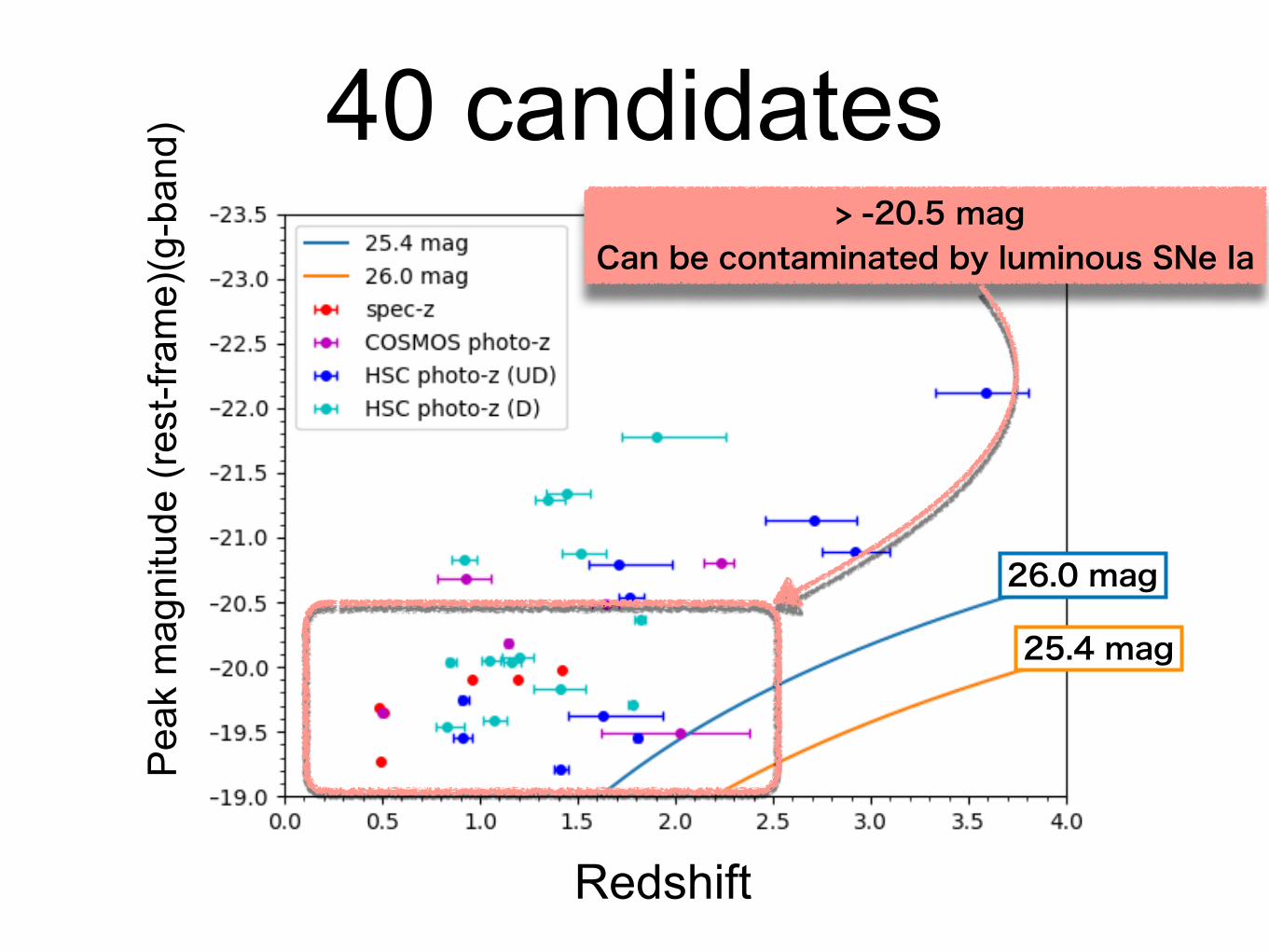
• spec-z or good photo-z with < 30% accuracy • Luminous (< -19.5 mag) • Enough number of detection (≧ 5) • Not SN Ia (by SN Ia fitting)


27


40


40 candidates

Redshift

Pea

k m

agni

tude

(res

t-fra

me)

(g-b

and)

26.0 mag

25.4 mag

40 candidates

Redshift

> -20.5 mag Can be contaminated by luminous SNe Ia

Pea

k m

agni

tude

(res

t-fra

me)

(g-b

and)

26.0 mag

25.4 mag


27


40

• 19 SNe (< -20.5 mag)→ OK • 21 SNe (> -20.5 mag)→ 2nd step


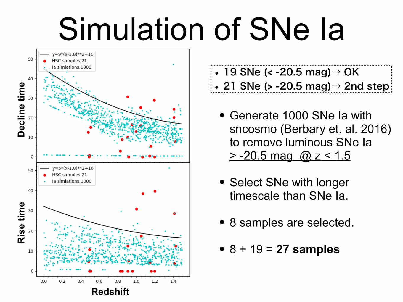
Simulation of SNe Ia

• Generate 1000 SNe Ia with sncosmo (Berbary et. al. 2016) to remove luminous SNe Ia > -20.5 mag @ z < 1.5

• Select SNe with longer timescale than SNe Ia.

• 8 samples are selected.

• 8 + 19 = 27 samples

Dec

line

time

Ris

e tim

e

Redshift


• Generate 1000 SNe Ia with sncosmo (Berbary et. al. 2016) to remove luminous SNe Ia > -20.5 mag @ z < 1.5

• Select SNe with longer timescale than SNe Ia.

• 8 samples are selected.

• 8 + 19 = 27 samples in total


Dec

line

time

Ris

e tim

e

Redshift

Simulation of SNe Ia




Pea

k m

agni

tude

(res

t-fra

me)

(g-b

and)

Redshift

Final samples of luminous CCSNe27 samples

Examples of Light Curve from HSC

※x-axis : Rest frame ※with simulated Ia SNe for compare

Days after maximum Days after maximum

Z = 0.929 Z =1.05

Abs

olut

e M

agni

tude

Event Rate =N

ϵ * V * t

V =43

πD3co

ΩΩall

t =tobs

1 + z

(Rate of CCSN: Dahlen et. al. 2018, Gal-yam et. al. 2012 SLSN: Cooke et. al. 2012, Quimby et. al. 2013, Moriya et. al. 2019)

Even

t rat

e ![G

pc−

3 yr−

1 ]

z = 0.5 ~ 1.5

-19 -20 -21 -22Peak Magnitude

-22 -23-18-17

Normal SNe

Event rate at 0.5<z<1.5

My work

SLSNe

Z ~ 0

Z ~ 1

~ 2000 [Gpc-3yr-1]

Event Rate =N

ϵ * V * t

V =43

πD3co

ΩΩall

t =tobs

1 + z

(Rate of CCSN: Dahlen et. al. 2018, Gal-yam et. al. 2012 SLSN: Cooke et. al. 2012, Quimby et. al. 2013, Moriya et. al. 2019)

Even

t rat

e ![G

pc−

3 yr−

1 ]

z = 0.5 ~ 1.5

-19 -20 -21 -22Peak Magnitude

-22 -23-18-17

Normal SNe

Event rate at 0.5<z<1.5

My work

SLSNe

Continuous distribution

~ 2000 [Gpc-3yr-1]

Z ~ 1

Z ~ 0

Summary• Found 27 Luminous SNe

• -19.5 ~ -20.5 mag : 9 SNe

• -20.5 ~ -21.5 mag : 10 SNe

• event rate @0.5<z<1.5

• -19.5 ~ -20.5 mag : > 2000 [/Gpc3/yr]

• -20.5 ~ -21.5 mag : ~ 2000 [/Gpc3/yr]

• Continuous luminosity distribution

Normal SNe

My workSLSNe

Documents

Luminosity distribution of luminous SNe from HSC transient