Endpoint Strichartz estimates

Markus Keel and Terence Tao

(Amer. J. Math. 120 (1998) 955–980)

Presenter : Nobu Kishimoto (Kyoto University)

2013 Participating School in Analysis of PDE 2013/8/26–30, Jeju

1

Abstract of the paper

We prove an abstract Strichartz estimate, which implies previously unknown

endpoint Strichartz estimates for the wave equation (in dimension n ≥ 4) and

the Schrodinger equation (in dimension n ≥ 3).

Three other applications are discussed: local existence for a nonlinear wave

equation; and Strichartz-type estimates for more general dispersive equations

and for the kinetic transport equation.

2

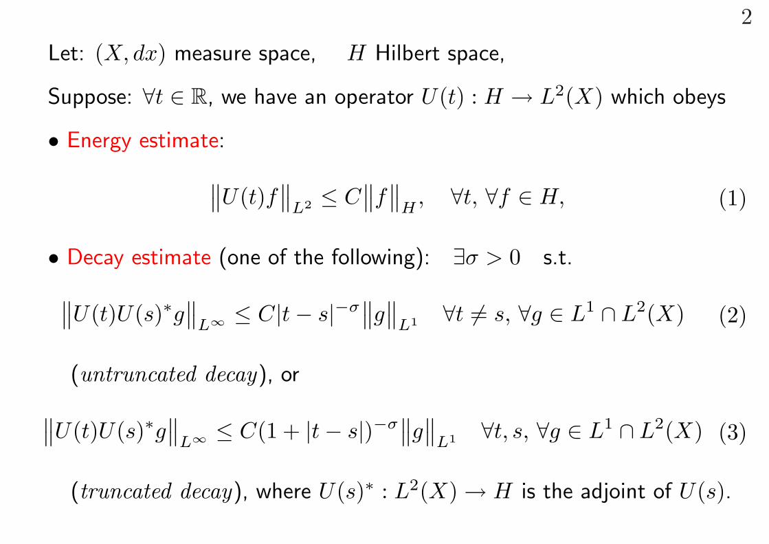
Let: (X, dx) measure space, H Hilbert space,

Suppose: ∀t ∈ R, we have an operator U(t) : H → L2(X) which obeys

• Energy estimate:∥∥U(t)f∥∥

L2 ≤ C∥∥f

∥∥H

, ∀t, ∀f ∈ H, (1)

• Decay estimate (one of the following): ∃σ > 0 s.t.∥∥U(t)U(s)∗g∥∥

L∞ ≤ C|t − s|−σ∥∥g

∥∥L1 ∀t 6= s, ∀g ∈ L1 ∩ L2(X) (2)

(untruncated decay), or∥∥U(t)U(s)∗g∥∥

L∞ ≤ C(1 + |t − s|)−σ∥∥g

∥∥L1 ∀t, s, ∀g ∈ L1 ∩ L2(X) (3)

(truncated decay), where U(s)∗ : L2(X) → H is the adjoint of U(s).

3

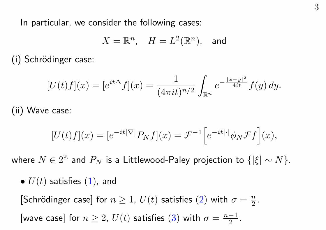
In particular, we consider the following cases:

X = Rn, H = L2(Rn), and

(i) Schrodinger case:

[U(t)f ](x) = [eit∆f ](x) =1

(4πit)n/2

∫Rn

e−|x−y|2

4it f(y) dy.

(ii) Wave case:

[U(t)f ](x) = [e−it|∇|PNf ](x) = F−1[e−it|·|φNFf

](x),

where N ∈ 2Z and PN is a Littlewood-Paley projection to {|ξ| ∼ N}.

• U(t) satisfies (1), and

[Schrodinger case] for n ≥ 1, U(t) satisfies (2) with σ = n2 .

[wave case] for n ≥ 2, U(t) satisfies (3) with σ = n−12 .

4

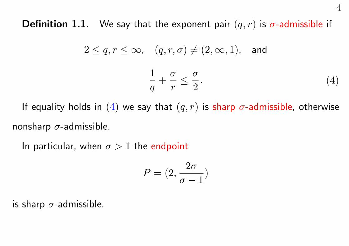
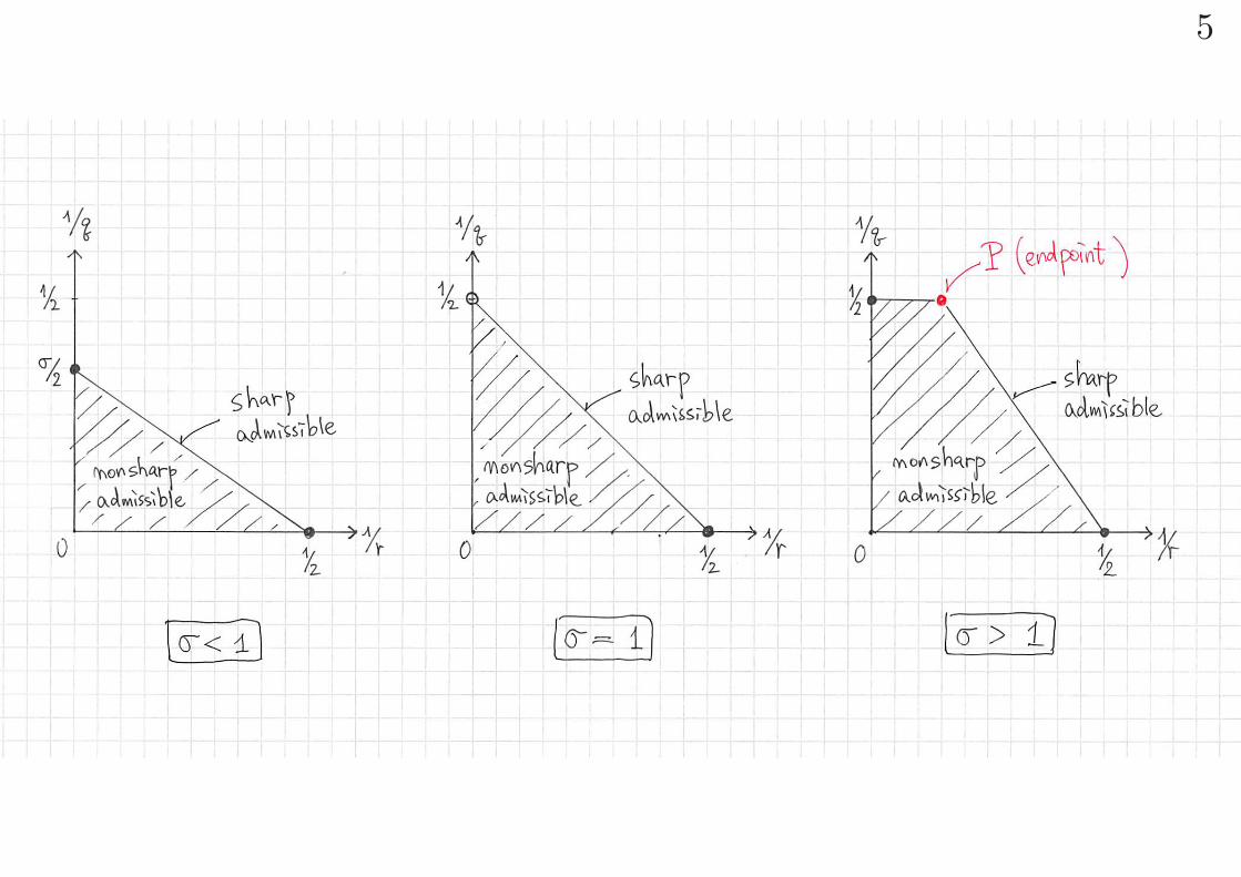
Definition 1.1. We say that the exponent pair (q, r) is σ-admissible if

2 ≤ q, r ≤ ∞, (q, r, σ) 6= (2,∞, 1), and

1q

+σ

r≤ σ

2. (4)

If equality holds in (4) we say that (q, r) is sharp σ-admissible, otherwise

nonsharp σ-admissible.

In particular, when σ > 1 the endpoint

P = (2,2σ

σ − 1)

is sharp σ-admissible.

5

6

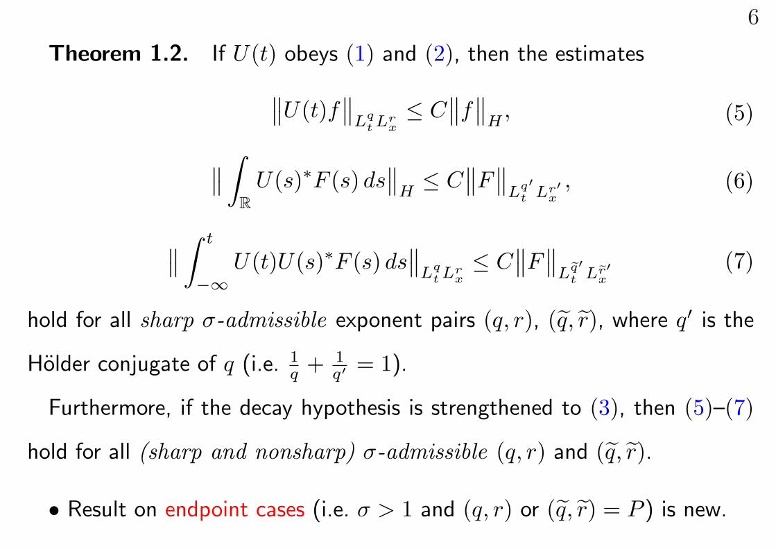
Theorem 1.2. If U(t) obeys (1) and (2), then the estimates∥∥U(t)f∥∥

Lqt Lr

x≤ C

∥∥f∥∥

H, (5)

∥∥ ∫R

U(s)∗F (s) ds∥∥

H≤ C

∥∥F∥∥

Lq′t Lr′

x, (6)

∥∥∫ t

−∞U(t)U(s)∗F (s) ds

∥∥Lq

t Lrx≤ C

∥∥F∥∥

Leq′t Ler′

x

(7)

hold for all sharp σ-admissible exponent pairs (q, r), (q, r), where q′ is the

Holder conjugate of q (i.e. 1q + 1

q′ = 1).

Furthermore, if the decay hypothesis is strengthened to (3), then (5)–(7)

hold for all (sharp and nonsharp) σ-admissible (q, r) and (q, r).

• Result on endpoint cases (i.e. σ > 1 and (q, r) or (q, r) = P ) is new.

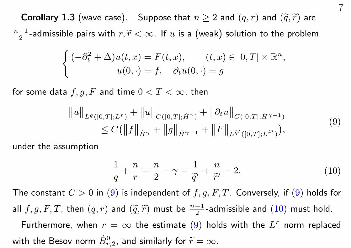
7Corollary 1.3 (wave case). Suppose that n ≥ 2 and (q, r) and (eq, er) are

n−12

-admissible pairs with r, er < ∞. If u is a (weak) solution to the problem

(

(−∂2t + ∆)u(t, x) = F (t, x), (t, x) ∈ [0, T ] × Rn,

u(0, ·) = f, ∂tu(0, ·) = g

for some data f, g, F and time 0 < T < ∞, then

‚

‚u‚

‚

Lq([0,T ];Lr)+

‚

‚u‚

‚

C([0,T ];Hγ)+

‚

‚∂tu‚

‚

C([0,T ];Hγ−1)

≤ C`

‚

‚f‚

‚

Hγ +‚

‚g‚

‚

Hγ−1 +‚

‚F‚

‚

Leq′ ([0,T ];Ler′ )

´

,(9)

under the assumption

1

q+

n

r=

n

2− γ =

1

eq′+

n

er′− 2. (10)

The constant C > 0 in (9) is independent of f, g, F, T . Conversely, if (9) holds for

all f, g, F, T , then (q, r) and (eq, er) must be n−12

-admissible and (10) must hold.

Furthermore, when r = ∞ the estimate (9) holds with the Lr norm replaced

with the Besov norm B0r,2, and similarly for er = ∞.

8

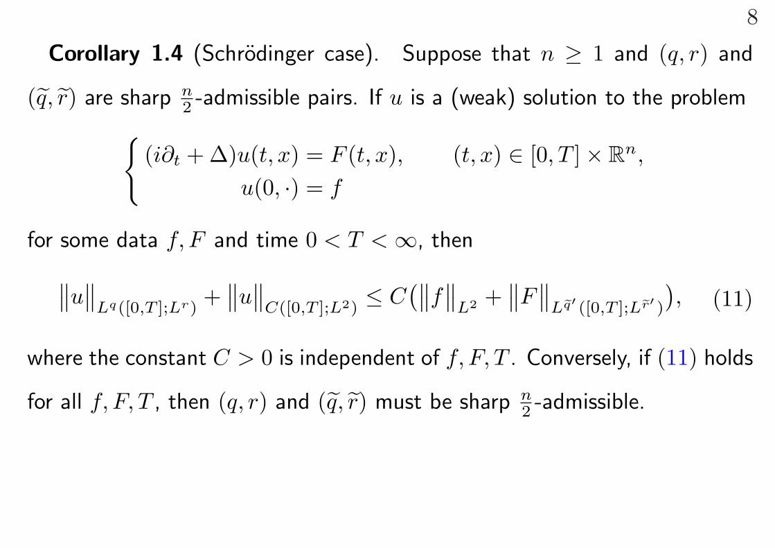
Corollary 1.4 (Schrodinger case). Suppose that n ≥ 1 and (q, r) and

(q, r) are sharp n2 -admissible pairs. If u is a (weak) solution to the problem{

(i∂t + ∆)u(t, x) = F (t, x), (t, x) ∈ [0, T ] × Rn,

u(0, ·) = f

for some data f, F and time 0 < T < ∞, then∥∥u∥∥

Lq([0,T ];Lr)+

∥∥u∥∥

C([0,T ];L2)≤ C

(∥∥f∥∥

L2 +∥∥F

∥∥Leq′ ([0,T ];Ler′ )

), (11)

where the constant C > 0 is independent of f, F, T . Conversely, if (11) holds

for all f, F, T , then (q, r) and (q, r) must be sharp n2 -admissible.

9

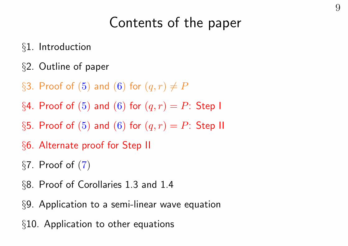
Contents of the paper

§1. Introduction

§2. Outline of paper

§3. Proof of (5) and (6) for (q, r) 6= P

§4. Proof of (5) and (6) for (q, r) = P : Step I

§5. Proof of (5) and (6) for (q, r) = P : Step II

§6. Alternate proof for Step II

§7. Proof of (7)

§8. Proof of Corollaries 1.3 and 1.4

§9. Application to a semi-linear wave equation

§10. Application to other equations

10

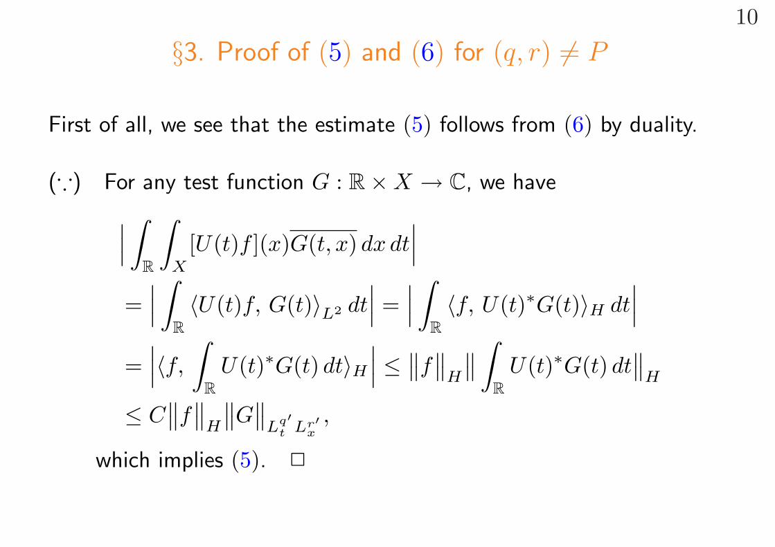
§3. Proof of (5) and (6) for (q, r) 6= P

First of all, we see that the estimate (5) follows from (6) by duality.

(∵) For any test function G : R × X → C, we have∣∣∣ ∫R

∫X

[U(t)f ](x)G(t, x) dx dt∣∣∣

=∣∣∣ ∫

R〈U(t)f, G(t)〉L2 dt

∣∣∣ =∣∣∣ ∫

R〈f, U(t)∗G(t)〉H dt

∣∣∣=

∣∣∣〈f,

∫R

U(t)∗G(t) dt〉H∣∣∣ ≤ ∥∥f

∥∥H

∥∥ ∫R

U(t)∗G(t) dt∥∥

H

≤ C∥∥f

∥∥H

∥∥G∥∥

Lq′t Lr′

x,

which implies (5). 2

11

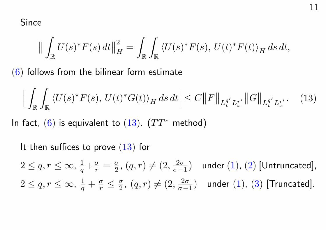
Since∥∥ ∫R

U(s)∗F (s) dt∥∥2

H=

∫R

∫R〈U(s)∗F (s), U(t)∗F (t)〉H ds dt,

(6) follows from the bilinear form estimate∣∣∣ ∫R

∫R〈U(s)∗F (s), U(t)∗G(t)〉H ds dt

∣∣∣ ≤ C∥∥F

∥∥Lq′

t Lr′x

∥∥G∥∥

Lq′t Lr′

x. (13)

In fact, (6) is equivalent to (13). (TT ∗ method)

It then suffices to prove (13) for

2 ≤ q, r ≤ ∞, 1q + σ

r = σ2 , (q, r) 6= (2, 2σ

σ−1 ) under (1), (2) [Untruncated],

2 ≤ q, r ≤ ∞, 1q + σ

r ≤ σ2 , (q, r) 6= (2, 2σ

σ−1 ) under (1), (3) [Truncated].

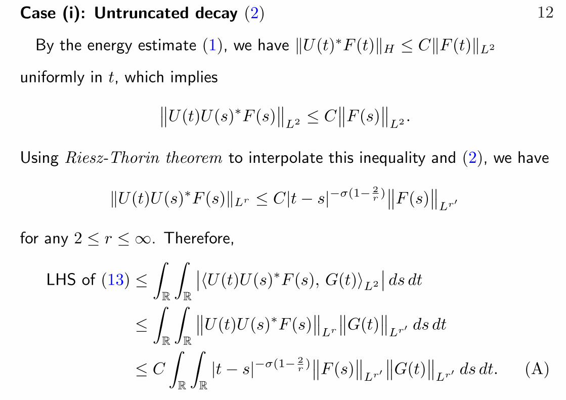
12Case (i): Untruncated decay (2)

By the energy estimate (1), we have ‖U(t)∗F (t)‖H ≤ C‖F (t)‖L2

uniformly in t, which implies∥∥U(t)U(s)∗F (s)∥∥

L2 ≤ C∥∥F (s)

∥∥L2 .

Using Riesz-Thorin theorem to interpolate this inequality and (2), we have

‖U(t)U(s)∗F (s)‖Lr ≤ C|t − s|−σ(1− 2r )

∥∥F (s)∥∥

Lr′

for any 2 ≤ r ≤ ∞. Therefore,

LHS of (13) ≤∫

R

∫R

∣∣〈U(t)U(s)∗F (s), G(t)〉L2

∣∣ ds dt

≤∫

R

∫R

∥∥U(t)U(s)∗F (s)∥∥

Lr

∥∥G(t)∥∥

Lr′ ds dt

≤ C

∫R

∫R|t − s|−σ(1− 2

r )∥∥F (s)

∥∥Lr′

∥∥G(t)∥∥

Lr′ ds dt. (A)

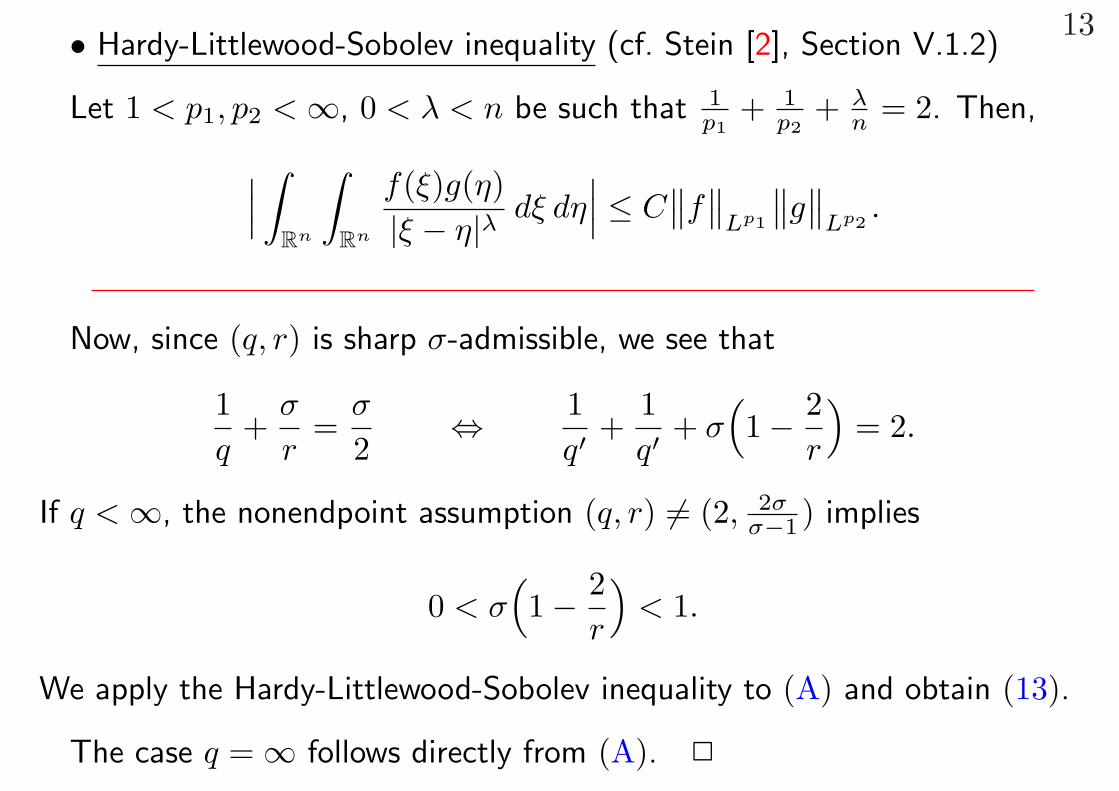
13• Hardy-Littlewood-Sobolev inequality (cf. Stein [2], Section V.1.2)

Let 1 < p1, p2 < ∞, 0 < λ < n be such that 1p1

+ 1p2

+ λn = 2. Then,∣∣∣ ∫

Rn

∫Rn

f(ξ)g(η)|ξ − η|λ

dξ dη∣∣∣ ≤ C

∥∥f∥∥

Lp1

∥∥g∥∥

Lp2.

Now, since (q, r) is sharp σ-admissible, we see that

1q

+σ

r=

σ

2⇔ 1

q′+

1q′

+ σ(1 − 2

r

)= 2.

If q < ∞, the nonendpoint assumption (q, r) 6= (2, 2σσ−1 ) implies

0 < σ(1 − 2

r

)< 1.

We apply the Hardy-Littlewood-Sobolev inequality to (A) and obtain (13).

The case q = ∞ follows directly from (A). 2

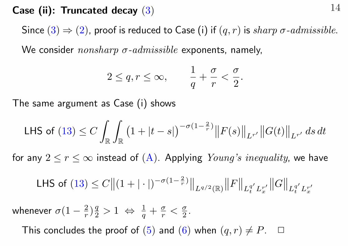
14Case (ii): Truncated decay (3)

Since (3) ⇒ (2), proof is reduced to Case (i) if (q, r) is sharp σ-admissible.

We consider nonsharp σ-admissible exponents, namely,

2 ≤ q, r ≤ ∞,1q

+σ

r<

σ

2.

The same argument as Case (i) shows

LHS of (13) ≤ C

∫R

∫R

(1 + |t − s|

)−σ(1− 2r )∥∥F (s)

∥∥Lr′

∥∥G(t)∥∥

Lr′ ds dt

for any 2 ≤ r ≤ ∞ instead of (A). Applying Young’s inequality, we have

LHS of (13) ≤ C∥∥(1 + | · |)−σ(1− 2

r )∥∥

Lq/2(R)

∥∥F∥∥

Lq′t Lr′

x

∥∥G∥∥

Lq′t Lr′

x

whenever σ(1 − 2r ) q

2 > 1 ⇔ 1q + σ

r < σ2 .

This concludes the proof of (5) and (6) when (q, r) 6= P . 2

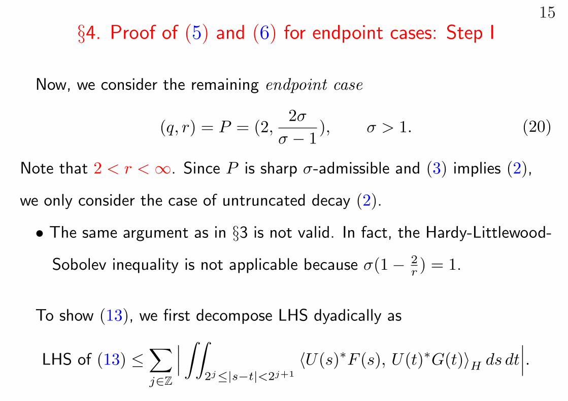
15§4. Proof of (5) and (6) for endpoint cases: Step I

Now, we consider the remaining endpoint case

(q, r) = P = (2,2σ

σ − 1), σ > 1. (20)

Note that 2 < r < ∞. Since P is sharp σ-admissible and (3) implies (2),

we only consider the case of untruncated decay (2).

• The same argument as in §3 is not valid. In fact, the Hardy-Littlewood-

Sobolev inequality is not applicable because σ(1 − 2r ) = 1.

To show (13), we first decompose LHS dyadically as

LHS of (13) ≤∑j∈Z

∣∣∣ ∫∫2j≤|s−t|<2j+1

〈U(s)∗F (s), U(t)∗G(t)〉H ds dt∣∣∣.

16By symmetry it suffices to show∑

j∈Z|Tj(F,G)| ≤ C

∥∥F∥∥

Lq′t Lr′

x

∥∥G∥∥

Lq′t Lr′

x, (22)

where

Tj(F,G) =∫∫

t−2j+1<s≤t−2j

〈U(s)∗F (s), U(t)∗G(t)〉H ds dt. (21)

The goal of Step I is the following two-parameter family of estimates:

Lemma 4.1. Assume (20). The estimate

|Tj(F,G)| ≤ C2−j{σ−1−σ( 1a + 1

b )}∥∥F∥∥

L2t La′

x

∥∥G∥∥

L2t Lb′

x(23)

holds (uniformly) for all j ∈ Z and all ( 1a , 1

b ) in a neighborhood of ( 1r , 1

r ).

• Since σ − 1 − σ( 1r + 1

r ) = 0, we have (22) with∑

j replaced by supj .

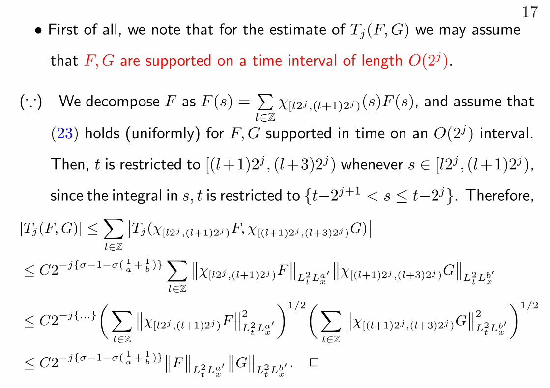
17• First of all, we note that for the estimate of Tj(F,G) we may assume

that F,G are supported on a time interval of length O(2j).

(∵) We decompose F as F (s) =∑l∈Z

χ[l2j ,(l+1)2j)(s)F (s), and assume that

(23) holds (uniformly) for F,G supported in time on an O(2j) interval.

Then, t is restricted to [(l+1)2j , (l+3)2j) whenever s ∈ [l2j , (l+1)2j),

since the integral in s, t is restricted to {t−2j+1 < s ≤ t−2j}. Therefore,

|Tj(F, G)| ≤X

l∈Z

˛

˛Tj(χ[l2j ,(l+1)2j)F, χ[(l+1)2j ,(l+3)2j)G)˛

˛

≤ C2−j{σ−1−σ( 1a

+ 1b)}

X

l∈Z

‚

‚χ[l2j ,(l+1)2j)F‚

‚

L2t La′

x

‚

‚χ[(l+1)2j ,(l+3)2j)G‚

‚

L2t Lb′

x

≤ C2−j{...}„

X

l∈Z

‚

‚χ[l2j ,(l+1)2j)F‚

‚

2

L2t La′

x

«1/2„

X

l∈Z

‚

‚χ[(l+1)2j ,(l+3)2j)G‚

‚

2

L2t Lb′

x

«1/2

≤ C2−j{σ−1−σ( 1a

+ 1b)}‚

‚F‚

‚

L2t La′

x

‚

‚G‚

‚

L2t Lb′

x. 2

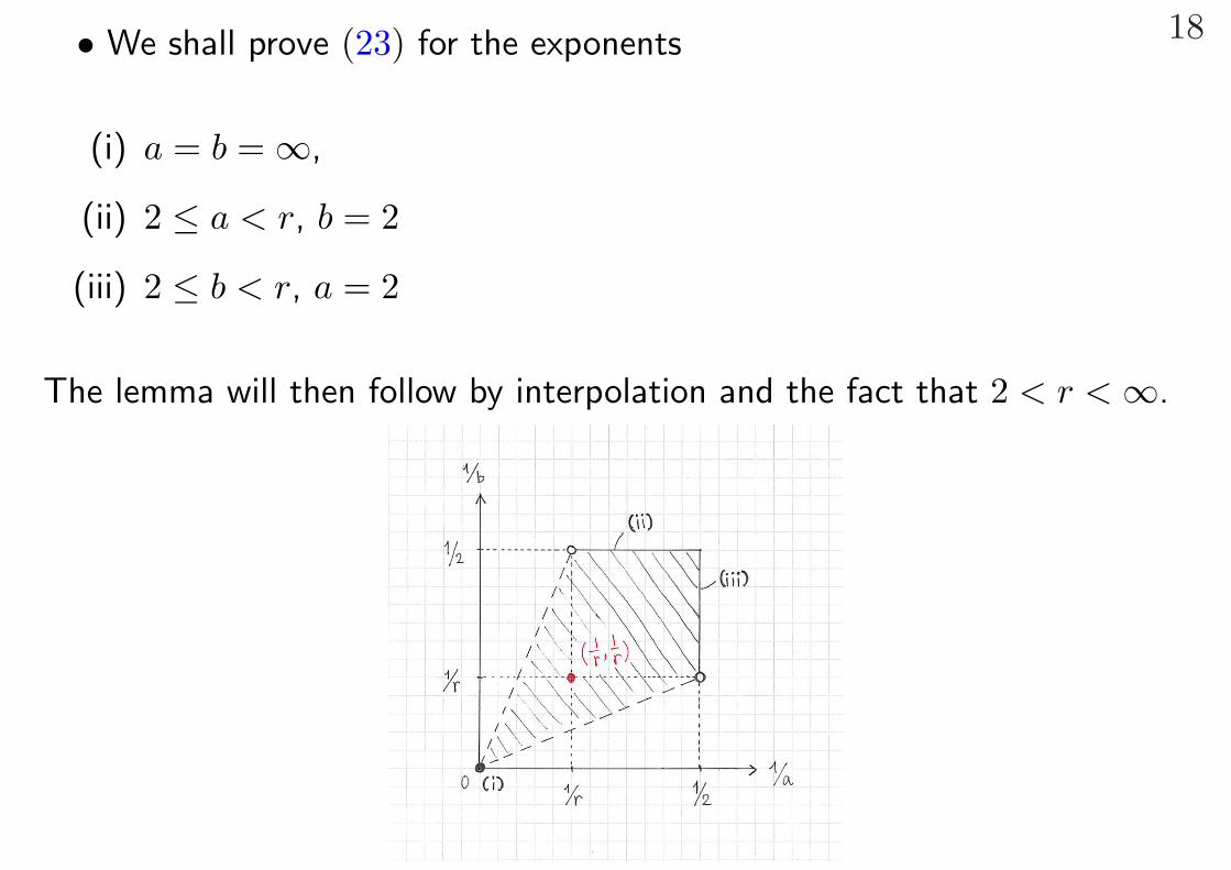
18• We shall prove (23) for the exponents

(i) a = b = ∞,

(ii) 2 ≤ a < r, b = 2

(iii) 2 ≤ b < r, a = 2

The lemma will then follow by interpolation and the fact that 2 < r < ∞.

19

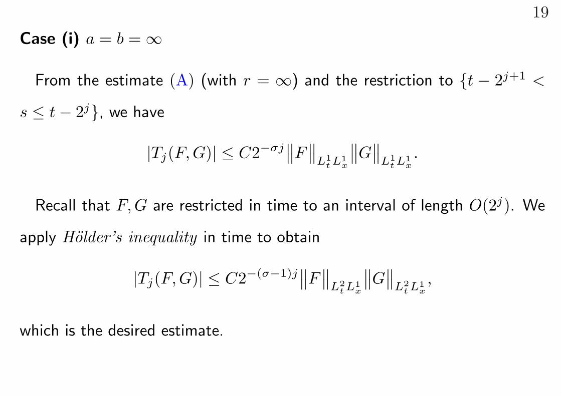
Case (i) a = b = ∞

From the estimate (A) (with r = ∞) and the restriction to {t − 2j+1 <

s ≤ t − 2j}, we have

|Tj(F,G)| ≤ C2−σj∥∥F

∥∥L1

t L1x

∥∥G∥∥

L1t L1

x.

Recall that F,G are restricted in time to an interval of length O(2j). We

apply Holder’s inequality in time to obtain

|Tj(F,G)| ≤ C2−(σ−1)j∥∥F

∥∥L2

t L1x

∥∥G∥∥

L2t L1

x,

which is the desired estimate.

20

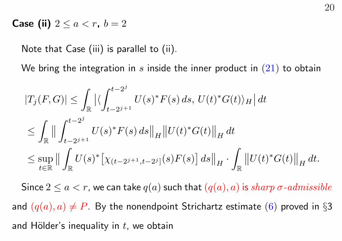
Case (ii) 2 ≤ a < r, b = 2

Note that Case (iii) is parallel to (ii).

We bring the integration in s inside the inner product in (21) to obtain

|Tj(F,G)| ≤∫

R

∣∣〈∫ t−2j

t−2j+1U(s)∗F (s) ds, U(t)∗G(t)〉H

∣∣ dt

≤∫

R

∥∥∫ t−2j

t−2j+1U(s)∗F (s) ds

∥∥H

∥∥U(t)∗G(t)∥∥

Hdt

≤ supt∈R

∥∥∫R

U(s)∗[χ(t−2j+1,t−2j ](s)F (s)

]ds

∥∥H·∫

R

∥∥U(t)∗G(t)∥∥

Hdt.

Since 2 ≤ a < r, we can take q(a) such that (q(a), a) is sharp σ-admissible

and (q(a), a) 6= P . By the nonendpoint Strichartz estimate (6) proved in §3

and Holder’s inequality in t, we obtain

21∥∥ ∫R

U(s)∗[χ(t−2j+1,t−2j ](s)F (s)

]ds

∥∥H

≤ C∥∥χ(t−2j+1,t−2j ]F

∥∥L

q(a)′t La′

x

≤ C2j( 1q(a)′ −

12 )∥∥F

∥∥L2

t La′x

,

uniformly in t.

By the energy estimate (1) and Holder’s inequality in t, we have∫R

∥∥U(t)∗G(t)∥∥

Hdt ≤ C

∥∥G∥∥

L1t L2

x≤ C2j/2

∥∥G∥∥

L2t L2

x.

Combining these estimates, we have

|Tj(F,G)| ≤ C2j/q(a)′∥∥F

∥∥L2

t La′x

∥∥G∥∥

L2t L2

x.

This is nothing but (23), since

1q(a)′

= 1 − 1q(a)

= 1 − σ(12− 1

a

)= −

(σ − 1 − σ

(1a

+12))

. 2

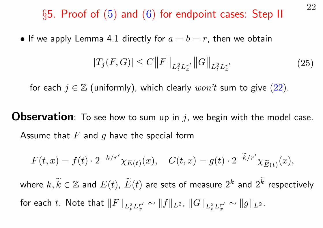
22§5. Proof of (5) and (6) for endpoint cases: Step II

• If we apply Lemma 4.1 directly for a = b = r, then we obtain

|Tj(F,G)| ≤ C∥∥F

∥∥L2

t Lr′x

∥∥G∥∥

L2t Lr′

x(25)

for each j ∈ Z (uniformly), which clearly won’t sum to give (22).

Observation: To see how to sum up in j, we begin with the model case.

Assume that F and g have the special form

F (t, x) = f(t) · 2−k/r′χE(t)(x), G(t, x) = g(t) · 2−ek/r′

χeE(t)(x),

where k, k ∈ Z and E(t), E(t) are sets of measure 2k and 2ek respectively

for each t. Note that ‖F‖L2t Lr′

x∼ ‖f‖L2 , ‖G‖L2

t Lr′x

∼ ‖g‖L2 .

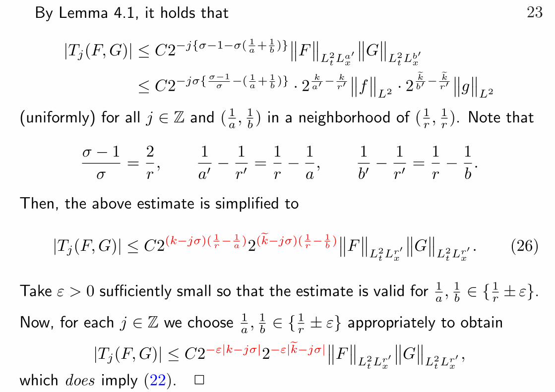
23By Lemma 4.1, it holds that

|Tj(F,G)| ≤ C2−j{σ−1−σ( 1a + 1

b )}∥∥F∥∥

L2t La′

x

∥∥G∥∥

L2t Lb′

x

≤ C2−jσ{σ−1σ −( 1

a + 1b )} · 2 k

a′ − kr′

∥∥f∥∥

L2 · 2ekb′ −

ekr′

∥∥g∥∥

L2

(uniformly) for all j ∈ Z and ( 1a , 1

b ) in a neighborhood of ( 1r , 1

r ). Note that

σ − 1σ

=2r,

1a′ −

1r′

=1r− 1

a,

1b′

− 1r′

=1r− 1

b.

Then, the above estimate is simplified to

|Tj(F,G)| ≤ C2(k−jσ)( 1r −

1a )2(ek−jσ)( 1

r −1b )

∥∥F∥∥

L2t Lr′

x

∥∥G∥∥

L2t Lr′

x. (26)

Take ε > 0 sufficiently small so that the estimate is valid for 1a , 1

b ∈ { 1r ± ε}.

Now, for each j ∈ Z we choose 1a , 1

b ∈ { 1r ± ε} appropriately to obtain

|Tj(F, G)| ≤ C2−ε|k−jσ|2−ε|ek−jσ|∥∥F

∥∥L2

t Lr′x

∥∥G∥∥

L2t Lr′

x,

which does imply (22). 2

24

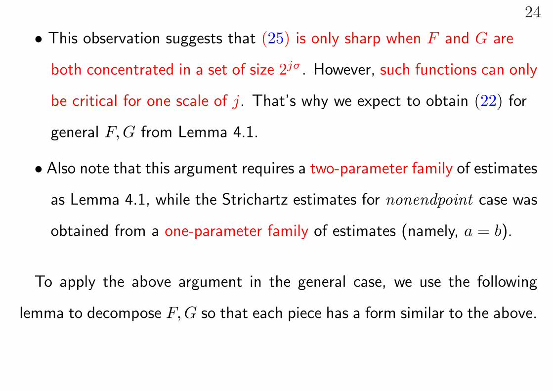
• This observation suggests that (25) is only sharp when F and G are

both concentrated in a set of size 2jσ. However, such functions can only

be critical for one scale of j. That’s why we expect to obtain (22) for

general F,G from Lemma 4.1.

• Also note that this argument requires a two-parameter family of estimates

as Lemma 4.1, while the Strichartz estimates for nonendpoint case was

obtained from a one-parameter family of estimates (namely, a = b).

To apply the above argument in the general case, we use the following

lemma to decompose F,G so that each piece has a form similar to the above.

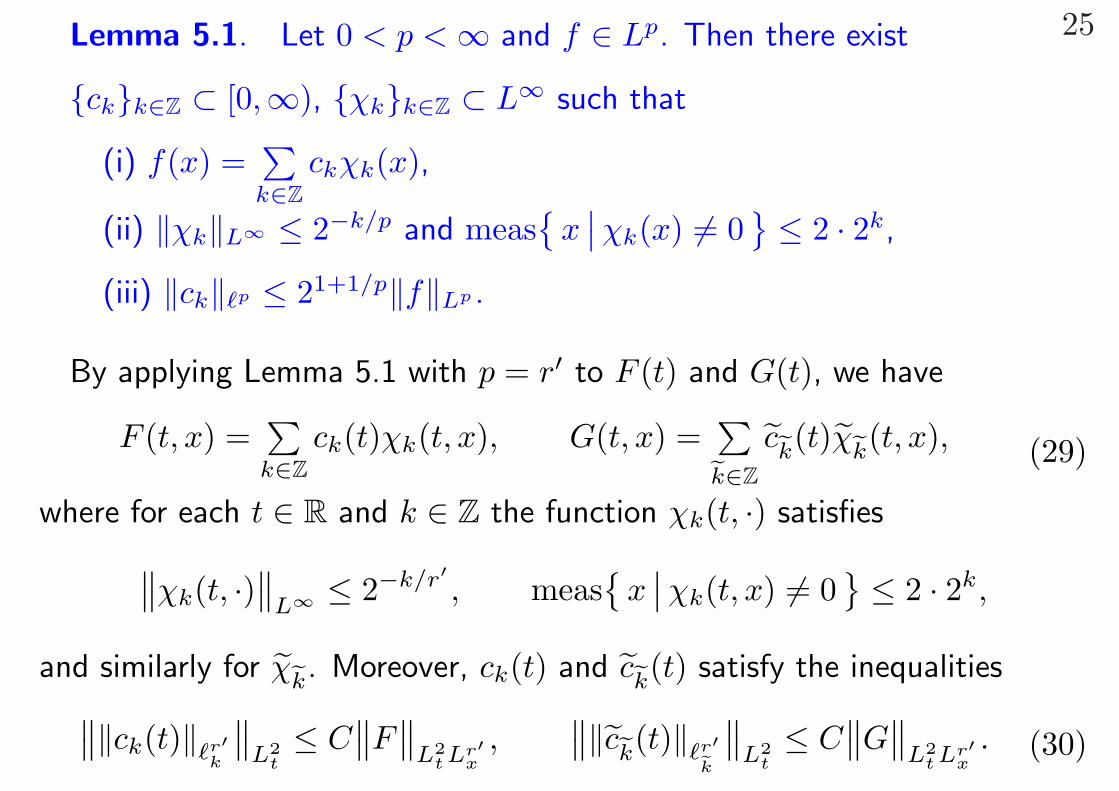
25Lemma 5.1. Let 0 < p < ∞ and f ∈ Lp. Then there exist

{ck}k∈Z ⊂ [0,∞), {χk}k∈Z ⊂ L∞ such that

(i) f(x) =∑k∈Z

ckχk(x),

(ii) ‖χk‖L∞ ≤ 2−k/p and meas{

x∣∣ χk(x) 6= 0

}≤ 2 · 2k,

(iii) ‖ck‖`p ≤ 21+1/p‖f‖Lp .

By applying Lemma 5.1 with p = r′ to F (t) and G(t), we have

F (t, x) =∑k∈Z

ck(t)χk(t, x), G(t, x) =∑

ek∈Zc

ek(t)χek(t, x), (29)

where for each t ∈ R and k ∈ Z the function χk(t, ·) satisfies∥∥χk(t, ·)∥∥

L∞ ≤ 2−k/r′, meas

{x

∣∣ χk(t, x) 6= 0}≤ 2 · 2k,

and similarly for χek. Moreover, ck(t) and c

ek(t) satisfy the inequalities∥∥‖ck(t)‖`r′k

∥∥L2

t≤ C

∥∥F∥∥

L2t Lr′

x,

∥∥‖cek(t)‖`r′

ek

∥∥L2

t≤ C

∥∥G∥∥

L2t Lr′

x. (30)

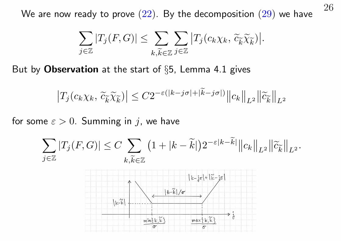
26We are now ready to prove (22). By the decomposition (29) we have∑

j∈Z|Tj(F, G)| ≤

∑k,ek∈Z

∑j∈Z

∣∣Tj(ckχk, cekχ

ek)∣∣.

But by Observation at the start of §5, Lemma 4.1 gives∣∣Tj(ckχk, cekχ

ek)∣∣ ≤ C2−ε(|k−jσ|+|ek−jσ|)∥∥ck

∥∥L2

∥∥cek

∥∥L2

for some ε > 0. Summing in j, we have∑j∈Z

|Tj(F, G)| ≤ C∑

k,ek∈Z

(1 + |k − k|

)2−ε|k−ek|∥∥ck

∥∥L2

∥∥cek

∥∥L2 .

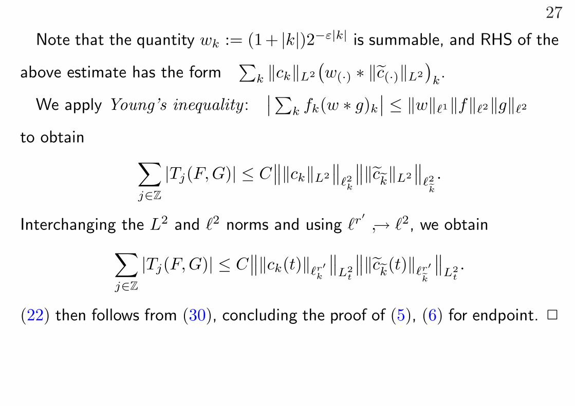
27

Note that the quantity wk := (1+ |k|)2−ε|k| is summable, and RHS of the

above estimate has the form∑

k ‖ck‖L2

(w(·) ∗ ‖c(·)‖L2

)k.

We apply Young’s inequality :∣∣ ∑

k fk(w ∗ g)k

∣∣ ≤ ‖w‖`1‖f‖`2‖g‖`2

to obtain ∑j∈Z

|Tj(F,G)| ≤ C∥∥‖ck‖L2

∥∥`2k

∥∥‖cek‖L2

∥∥`2

ek

.

Interchanging the L2 and `2 norms and using `r′↪→ `2, we obtain∑

j∈Z

|Tj(F,G)| ≤ C∥∥‖ck(t)‖`r′

k

∥∥L2

t

∥∥‖cek(t)‖`r′

ek

∥∥L2

t.

(22) then follows from (30), concluding the proof of (5), (6) for endpoint. 2

28

We now proceed to the proof of Lemma 5.1. Let f ∈ Lp, 0 < p < ∞.

Define the distribution function λ(α) of f for α ≥ 0 by

λ(α) = meas{

x∣∣ |f(x)| > α

}.

Note that λ(α) is non-increasing and right-continuous.

For each k ∈ Z, we set

αk = inf{

α > 0∣∣ λ(α) < 2k

}.

From definition we see that

0 ≤ αk < ∞, αk is non-increasing in k, limk→−∞

αk =∥∥f

∥∥L∞ ∈ [0,∞],

λ(αk) ≤ 2k, and λ(αk − 0) ≥ 2k if αk > 0. (B)

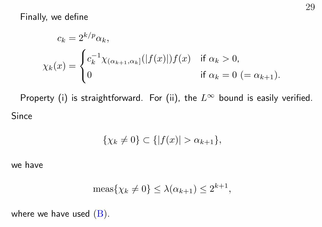
29Finally, we define

ck = 2k/pαk,

χk(x) =

c−1k χ(αk+1,αk](|f(x)|)f(x) if αk > 0,

0 if αk = 0 (= αk+1).

Property (i) is straightforward. For (ii), the L∞ bound is easily verified.

Since

{χk 6= 0} ⊂ {|f(x)| > αk+1},

we have

meas{χk 6= 0} ≤ λ(αk+1) ≤ 2k+1,

where we have used (B).

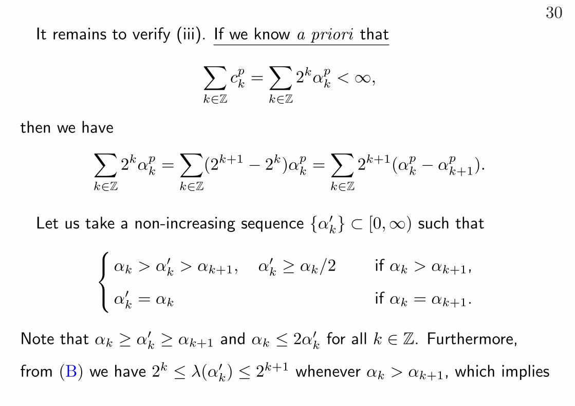
30It remains to verify (iii). If we know a priori that∑

k∈Z

cpk =

∑k∈Z

2kαpk < ∞,

then we have∑k∈Z

2kαpk =

∑k∈Z

(2k+1 − 2k)αpk =

∑k∈Z

2k+1(αpk − αp

k+1).

Let us take a non-increasing sequence {α′k} ⊂ [0,∞) such that αk > α′

k > αk+1, α′k ≥ αk/2 if αk > αk+1,

α′k = αk if αk = αk+1.

Note that αk ≥ α′k ≥ αk+1 and αk ≤ 2α′

k for all k ∈ Z. Furthermore,

from (B) we have 2k ≤ λ(α′k) ≤ 2k+1 whenever αk > αk+1, which implies

31∑k∈Z

2k(αpk − αp

k+1) ≤∑k∈Z

λ(α′k)(αp

k − αpk+1) ≤

∑k∈Z

2k+1(αpk − αp

k+1).

Since RHS is absolutely summable, we have∑k∈Z

2kαpk ≤ 2

∑k∈Z

λ(α′k)(αp

k − αpk+1)

= 2∑k∈Z

(λ(α′

k) − λ(α′k−1)

)αp

k

≤ 2 · 2p∑k∈Z

(λ(α′

k) − λ(α′k−1)

)(α′

k)p (∵ αk ≤ 2α′k)

= 21+p∑k∈Z

(α′k)p

∫{α′

k<|f(x)|≤α′k−1}

dx

≤ 21+p∥∥f

∥∥p

Lp ,

which shows (iii).

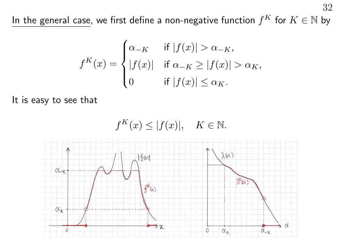
32In the general case, we first define a non-negative function fK for K ∈ N by

fK(x) =

α−K if |f(x)| > α−K ,

|f(x)| if α−K ≥ |f(x)| > αK ,

0 if |f(x)| ≤ αK .

It is easy to see that

fK(x) ≤ |f(x)|, K ∈ N.

33If we define the distribution function λK(α) and the sequence {αK

k }k∈Z

for each fK as before, then

λK(α) =

0 if α ≥ α−K ,

λ(α) if α−K > α ≥ αK ,

λ(αK) if α < αK ,

αKk =

0 if k > K,

αk if K ≥ k > −K,

α−K if k ≤ −K,

so that ∑k∈Z

2k(αKk )p =

∑−K<k≤K

2kαpk + α−K

∑k≤−K

2k < ∞

for any K ∈ N. Therefore, we can apply the previous argument and obtain∑−K<k≤K

2kαpk ≤

∑k∈Z

2k(αKk )p ≤ 21+p

∥∥fK∥∥p

Lp ≤ 21+p∥∥f

∥∥p

Lp .

Letting K → ∞ verifies (iii), which concludes the proof of Lemma 5.1. 2

34§6. Alternate proof for Step II

In §5, we have deduced the strong (`1j) summability in L2t L

r′

x × L2t L

r′

x

from the weak (`∞j ) summability in L2t L

a′

x ×L2t L

b′

x with (a, b) around (r, r).

Such a situation is similar to the Marcinkiewicz interpolation theorem,

which asserts that the strong boundedness

T : Lp → Lp

of an operator T is deduced from the weak boundedness

T : Lp1 → Lp1,∞, T : Lp2 → Lp2,∞

if 1 ≤ p1 < p < p2 ≤ ∞.

Marcinkiewicz interpolation theorem is one of the simplest consequences

in real interpolation theory. In fact, we can rephrase the previous derivation

of (22) from Lemma 4.1 by using existing results in real interpolation theory.

35

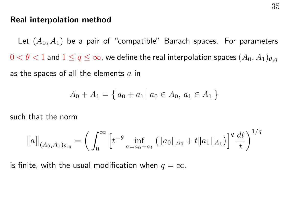
Real interpolation method

Let (A0, A1) be a pair of “compatible” Banach spaces. For parameters

0 < θ < 1 and 1 ≤ q ≤ ∞, we define the real interpolation spaces (A0, A1)θ,q

as the spaces of all the elements a in

A0 + A1 ={

a0 + a1

∣∣ a0 ∈ A0, a1 ∈ A1

}such that the norm

∥∥a∥∥

(A0,A1)θ,q=

(∫ ∞

0

[t−θ inf

a=a0+a1

(‖a0‖A0 + t‖a1‖A1

)]q dt

t

)1/q

is finite, with the usual modification when q = ∞.

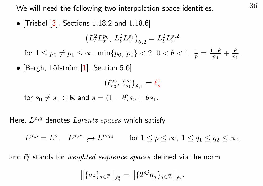
36We will need the following two interpolation space identities.

• [Triebel [3], Sections 1.18.2 and 1.18.6](L2

t Lp0x , L2

t Lp1x

)θ,2

= L2t L

p,2x

for 1 ≤ p0 6= p1 ≤ ∞, min{p0, p1} < 2, 0 < θ < 1, 1p = 1−θ

p0+ θ

p1.

• [Bergh, Lofstrom [1], Section 5.6](`∞s0

, `∞s1

)θ,1

= `1s

for s0 6= s1 ∈ R and s = (1 − θ)s0 + θs1.

Here, Lp,q denotes Lorentz spaces which satisfy

Lp,p = Lp, Lp,q1 ↪→ Lp,q2 for 1 ≤ p ≤ ∞, 1 ≤ q1 ≤ q2 ≤ ∞,

and `qs stands for weighted sequence spaces defined via the norm∥∥{aj}j∈Z

∥∥`q

s=

∥∥{2sjaj}j∈Z∥∥

`q .

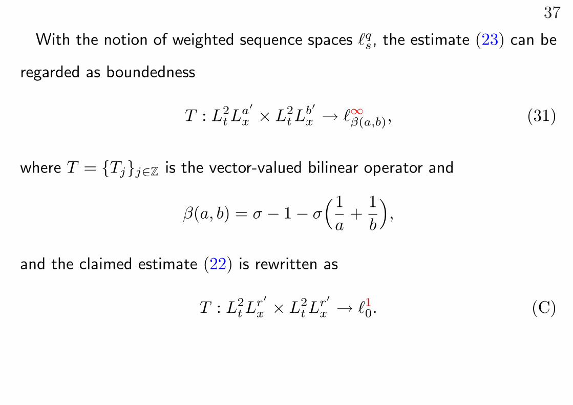
37

With the notion of weighted sequence spaces `qs, the estimate (23) can be

regarded as boundedness

T : L2t L

a′

x × L2t L

b′

x → `∞β(a,b), (31)

where T = {Tj}j∈Z is the vector-valued bilinear operator and

β(a, b) = σ − 1 − σ(1

a+

1b

),

and the claimed estimate (22) is rewritten as

T : L2t L

r′

x × L2t L

r′

x → `10. (C)

38

We will use the following bilinear interpolation theorem:

Lemma 6.1. ([1], Exercise 5(b) of Section 3.13)

Let (A0, A1), (B0, B1), (C0, C1) be “compatible” pairs of Banach spaces.

Suppose that the bilinear operator T is bounded as

T : A0 × B0 → C0, A1 × B0 → C1, A0 × B1 → C1.

Then, we have boundedness

T :(A0, A1

)θA,pAq

×(B0, B1

)θB ,pBq

→(C0, C1

)θ,q

whenever

0 < θA, θB < θ = θA + θB < 1, 1 ≤ pA, pB , q ≤ ∞,1pA

+1

pB≥ 1.

39We set, with ε > 0 sufficiently small,

A0 = B0 = L2t L

a′0

x , A1 = B1 = L2t L

a′1

x ,1a0

=1r− ε,

1a1

=1r

+ 2ε.

Then, by Lemma 4.1 (or (31)) the assumption in Lemma 6.1 is satisfied with

C0 = `∞2σε, C1 = `∞−σε.

We apply Lemma 6.1 with

θA = θB =13, pA = pB = 2, q = 1

to obtain the boundedness

T : L2t L

r′,2x × L2

t Lr′,2x → `10,

which implies the claim (C) because of the embedding Lr′↪→ Lr′,2. 2

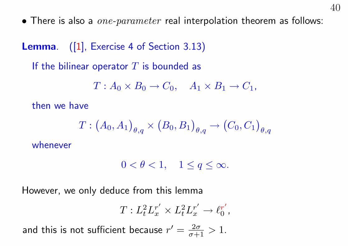
40• There is also a one-parameter real interpolation theorem as follows:

Lemma. ([1], Exercise 4 of Section 3.13)

If the bilinear operator T is bounded as

T : A0 × B0 → C0, A1 × B1 → C1,

then we have

T :(A0, A1

)θ,q

×(B0, B1

)θ,q

→(C0, C1

)θ,q

whenever

0 < θ < 1, 1 ≤ q ≤ ∞.

However, we only deduce from this lemma

T : L2t L

r′

x × L2t L

r′

x → `r′

0 ,

and this is not sufficient because r′ = 2σσ+1 > 1.

References

41

References

[1] J. Bergh and J. Lofstrom, Interpolation Spaces: An Introduction,

Springer-Verlag, New York, 1976.

[2] E. Stein, Singular Integrals and Differentiability Properties of Func-

tions, Princeton University Press, 1970.

[3] H. Triebel, Interpolation Theory, Function Spaces, Differential Opera-

tors, North-Holland, New York, 1978.

Thank you for your attention !