Embed Size (px)
Citation preview
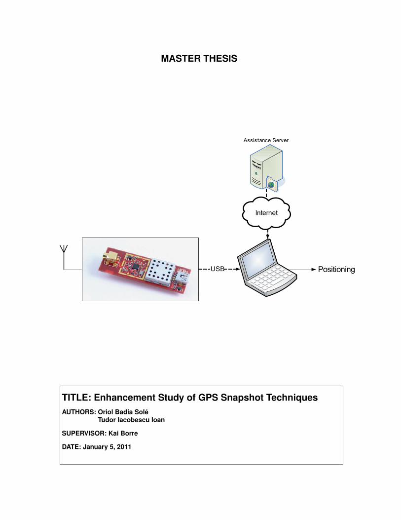
MASTER THESIS
PositioningUSB
Internet
Assistance Server
TITLE: Enhancement Study of GPS Snapshot TechniquesAUTHORS: Oriol Badia Sole
Tudor Iacobescu Ioan
SUPERVISOR: Kai Borre
DATE: January 5, 2011

Studyboard for Danish GPS Center
Fredrik Bajers Vej 7 B4-207, 9220 Aalborg Ø
Telephone +45 9940 8714
www.esn.aau.dk
Title
Enhancement Study ofGPS Snapshot Techniques
Type
Master Thesis for GPS technology
Period
1st September 2010 to5th January 2011
Semester and group
10th semester, GPS technology,group 1230
Participants
Tudor Iacobescu Ioan
Oriol Badia Solé
Supervisor
Kai Borre
Copies: 4
Pages: 63 (appendix: 5)
CD included
Webpage: kom.aau.dk/group/10gr1230/
e-mail: [email protected]
Synopsis
GPS snapshot techniques are becoming more and
more popular in the scienti�c community mostly
due to the fact that they involve minimizing
hardware components and reducing power con-
sumption, both aspects leading to dramatic cost
reductions.
The motivation of the present project is to
provide new functionality to GPS snapshot
techniques. We focused on two main directions:
improving position accuracy and making the
application available for non-experienced users
by automatically providing necessary assistance
data.
These concepts are approached by automating
the process of providing assisted data, by ana-
lyzing, implementing, and comparing di�erent
tracking algorithms and pseudo-range corrections.
Our results demonstrate improvements in accu-
racy levels and energy consumption.


Acknowledgements
We would like to take this opportunity to express our gratitude and appreciation to all the peoplewho assisted us in preparation of this thesis and who have made our overall experience at DGCboth fun and challenging.
We would like to thank Prof. Dr. Kai Borre and to Dr. Darius Plausinaitis for the theoreticaland technical insights they have shared, and in general for all the help they have provided. Wewould also like to thank the entire DGC for providing us with all the necessary equipment andtools that made the realization of this project possible.
Last, but not least, we would also like to thank our families for all the support andencouragement they have provided all along our stay in Aalborg University.


CONTENTS
INTRODUCTION . . . . . . . . . . . . . . . . . . . . . . . . . . . . . . . . . . . . . . . . 1
CHAPTER 1. Problem Formulation . . . . . . . . . . . . . . . . . . . . . . . . . . 3
1.1 Previous Results . . . . . . . . . . . . . . . . . . . . . . . . . . . . . . . . . . . . . . . 3
1.2 Future Tendencies . . . . . . . . . . . . . . . . . . . . . . . . . . . . . . . . . . . . . . 3
1.3 Problem Identification . . . . . . . . . . . . . . . . . . . . . . . . . . . . . . . . . . . 4
1.4 Project Scope . . . . . . . . . . . . . . . . . . . . . . . . . . . . . . . . . . . . . . . . 4
1.5 Final Problem Formulation . . . . . . . . . . . . . . . . . . . . . . . . . . . . . . . . . 5
CHAPTER 2. Analysis . . . . . . . . . . . . . . . . . . . . . . . . . . . . . . . . . . . 7
2.1 Overall Positioning Accuracy . . . . . . . . . . . . . . . . . . . . . . . . . . . . . . . 72.1.1 Signal Tracking . . . . . . . . . . . . . . . . . . . . . . . . . . . . . . . . . . . 72.1.2 Pseudo-Range Error Budget . . . . . . . . . . . . . . . . . . . . . . . . . . . . 9
2.2 Assistance Data . . . . . . . . . . . . . . . . . . . . . . . . . . . . . . . . . . . . . . . 122.2.1 Mandatory Assistance Data . . . . . . . . . . . . . . . . . . . . . . . . . . . . 122.2.2 Supplementary Assistance Data . . . . . . . . . . . . . . . . . . . . . . . . . 12
2.3 Summary . . . . . . . . . . . . . . . . . . . . . . . . . . . . . . . . . . . . . . . . . . . 13
CHAPTER 3. Development . . . . . . . . . . . . . . . . . . . . . . . . . . . . . . . . 15
3.1 Improving Accuracy . . . . . . . . . . . . . . . . . . . . . . . . . . . . . . . . . . . . . 153.1.1 Signal Tracking . . . . . . . . . . . . . . . . . . . . . . . . . . . . . . . . . . . 153.1.2 Pseudo-range Corrections . . . . . . . . . . . . . . . . . . . . . . . . . . . . . 193.1.3 Weighted Least Squares . . . . . . . . . . . . . . . . . . . . . . . . . . . . . . 24
3.2 Auto-Assistance . . . . . . . . . . . . . . . . . . . . . . . . . . . . . . . . . . . . . . . 273.2.1 Assisted Time . . . . . . . . . . . . . . . . . . . . . . . . . . . . . . . . . . . . 273.2.2 Ephemerides . . . . . . . . . . . . . . . . . . . . . . . . . . . . . . . . . . . . 343.2.3 Computing First Fix from Doppler Measurements . . . . . . . . . . . . . . . . 34
3.3 Summary . . . . . . . . . . . . . . . . . . . . . . . . . . . . . . . . . . . . . . . . . . . 36
CHAPTER 4. Experimental Results . . . . . . . . . . . . . . . . . . . . . . . . . . 39
4.1 Energy Saving . . . . . . . . . . . . . . . . . . . . . . . . . . . . . . . . . . . . . . . . 39
4.2 Accuracy Improvement . . . . . . . . . . . . . . . . . . . . . . . . . . . . . . . . . . . 404.2.1 Tracking results . . . . . . . . . . . . . . . . . . . . . . . . . . . . . . . . . . . 404.2.2 Pseudo-range Corrections . . . . . . . . . . . . . . . . . . . . . . . . . . . . . 414.2.3 Weighted Least Squares . . . . . . . . . . . . . . . . . . . . . . . . . . . . . . 47
4.3 Summary . . . . . . . . . . . . . . . . . . . . . . . . . . . . . . . . . . . . . . . . . . . 47

CHAPTER 5. Implementation Discussion . . . . . . . . . . . . . . . . . . . . . 49
CHAPTER 6. Conclusions . . . . . . . . . . . . . . . . . . . . . . . . . . . . . . . . 51
CHAPTER 7. Future work . . . . . . . . . . . . . . . . . . . . . . . . . . . . . . . . 53
APPENDIX A. Previous Results . . . . . . . . . . . . . . . . . . . . . . . . . . . . . 57
APPENDIX B. Glossary . . . . . . . . . . . . . . . . . . . . . . . . . . . . . . . . . . . 59
APPENDIX C. Group Dynamics . . . . . . . . . . . . . . . . . . . . . . . . . . . . . 61
BIBLIOGRAPHY . . . . . . . . . . . . . . . . . . . . . . . . . . . . . . . . . . . . . . . . 63
LIST OF FIGURES
1.1 Project Gantt diagram. Blue symbolizes development time, red means the time spenton the report writing and yellow suggests a time margin we have allowed for furtherexperiments. . . . . . . . . . . . . . . . . . . . . . . . . . . . . . . . . . . . . . . . . . 5
2.1 Basic demodulation scheme . . . . . . . . . . . . . . . . . . . . . . . . . . . . . . . . . 72.2 Phasor diagram . . . . . . . . . . . . . . . . . . . . . . . . . . . . . . . . . . . . . . . . 82.3 Costas Loop block diagram . . . . . . . . . . . . . . . . . . . . . . . . . . . . . . . . . . 82.4 Early-Late DLL . . . . . . . . . . . . . . . . . . . . . . . . . . . . . . . . . . . . . . . . 92.5 Early-Prompt-Late correlation . . . . . . . . . . . . . . . . . . . . . . . . . . . . . . . . 9
3.1 Discriminator output versus code error . . . . . . . . . . . . . . . . . . . . . . . . . . . 163.2 Block diagram of combined DLL and PLL tracking loops [1] . . . . . . . . . . . . . . . 173.3 Code phase measurements relative to common measuring point . . . . . . . . . . . . . 183.4 Raw DLL discriminator output . . . . . . . . . . . . . . . . . . . . . . . . . . . . . . . 183.5 Discriminator output versus true error . . . . . . . . . . . . . . . . . . . . . . . . . . . 193.6 Raw DLL discriminator output observed for 7 ms . . . . . . . . . . . . . . . . . . . . . 193.7 Basic tasks needed to solve for ionospheric delay . . . . . . . . . . . . . . . . . . . . . . 203.8 IPP computation [2] . . . . . . . . . . . . . . . . . . . . . . . . . . . . . . . . . . . . . 213.9 Bivariate interpolation using the 4 nearest TEC points [3] . . . . . . . . . . . . . . . . 223.10 Number of coincident satellites along day . . . . . . . . . . . . . . . . . . . . . . . . . . 293.11 Distance residuals during a day . . . . . . . . . . . . . . . . . . . . . . . . . . . . . . . 313.12 Distance residuals within fine time interval . . . . . . . . . . . . . . . . . . . . . . . . . 313.13 Flow diagram of TW computation using ephemeris and user coordinates . . . . . . . . 33
4.1 GPS1A hardware block . . . . . . . . . . . . . . . . . . . . . . . . . . . . . . . . . . . . 394.2 Solar Cycles 23-24 . . . . . . . . . . . . . . . . . . . . . . . . . . . . . . . . . . . . . . . 424.3 Pseudo-range corrections effects for “O1D”; SA enabled . . . . . . . . . . . . . . . . . 434.4 Horizontal accuracy improvement for “O4D” . . . . . . . . . . . . . . . . . . . . . . . . 444.5 Horizontal accuracy improvement for “O2D” and “O3E” . . . . . . . . . . . . . . . . . 444.6 Vertical Positioning Error vs. Time for “O2D” and “O3E” . . . . . . . . . . . . . . . . 454.7 HPE histograms before and after corrections for “O2D” . . . . . . . . . . . . . . . . . 454.8 VPE histograms before and after corrections for “O2D” . . . . . . . . . . . . . . . . . 46
7.1 Current basic system architecture . . . . . . . . . . . . . . . . . . . . . . . . . . . . . 537.2 Prototype basic system architecture . . . . . . . . . . . . . . . . . . . . . . . . . . . . 53
A.1 Google Earth plot of apriori coordinates used to test the algorithm . . . . . . . . . . . 58A.2 Distance between fix and real coordinates versus bias on assisted time . . . . . . . . . 58


LIST OF TABLES
2.1 Error Sources Outline . . . . . . . . . . . . . . . . . . . . . . . . . . . . . . . . . . . . . 13
3.1 Average meteorological parameters for tropospheric delay . . . . . . . . . . . . . . . . 23
3.2 Seasonal variation of meteorological parameters for tropospheric delay . . . . . . . . . 23
3.3 Relationship between URA index and URA of the satellite (taken from [3]) . . . . . . . 26
3.4 GPS satellite combinations . . . . . . . . . . . . . . . . . . . . . . . . . . . . . . . . . . 303.5 TW estimation results . . . . . . . . . . . . . . . . . . . . . . . . . . . . . . . . . . . . 32
4.1 GPS1A power consumption . . . . . . . . . . . . . . . . . . . . . . . . . . . . . . . . . 39
4.2 Typical TTFF for different types of stars. . . . . . . . . . . . . . . . . . . . . . . . . . 40
4.3 Error statistics for acquisition and/or tracking based positioning . . . . . . . . . . . . . 404.4 Observations set . . . . . . . . . . . . . . . . . . . . . . . . . . . . . . . . . . . . . . . . 41
4.5 Correction levels . . . . . . . . . . . . . . . . . . . . . . . . . . . . . . . . . . . . . . . . 424.6 Positioning statistics . . . . . . . . . . . . . . . . . . . . . . . . . . . . . . . . . . . . . 464.7 Weighted least squares positioning statistics . . . . . . . . . . . . . . . . . . . . . . . . 47
A.1 Snapshots specifications . . . . . . . . . . . . . . . . . . . . . . . . . . . . . . . . . . . 57
A.2 Positioning statistics from snapshot “S1D” . . . . . . . . . . . . . . . . . . . . . . . . . 57
B.1 Abbreviations used in the report in alphabetical order . . . . . . . . . . . . . . . . . . 59

1
INTRODUCTION
The GPS system was created in order to satisfy the need of several U.S. governmental institutionsand organizations such as Department of Defence (DoD), the National Aeronautics and SpaceAdministration (NASA) agency and the Department of Transportation, for a three-dimensionalpositioning system which would be able to provide [4]:
• Global coverage
• Continuity
• Availability
• Capability to serve high dynamical platforms
Despite its military origin, a civilian signal was also included in the original design. Initially, theaccuracy of this signal was degraded and controlled through Selective Availability (SA). HoweverSA was removed in the year 2000, leading to an explosion of civilian applications. Nowadays GPS isused for a great variety of civil and scientific applications which include: position and navigation,land surveying (from cartography to monitoring of tectonic plates movement), animal tracking,troposphere and ionosphere monitoring and timing synchronization of network equipments.
The first mainstream application that really spiked the interest of the general public was theportable car navigator, which enabled its user to visualize his/her position on a map, plan aroute and get driving directions to the destination. Since then, this field witnessed a continuousgrowth, bringing GPS uses into everyday life. Perhaps, the last important boost in mass-marketapplications is the creation of A-GPS (Assisted-GPS), pushed by the U.S. Federal CommunicationsCommission, which was aiming to provide position information for the 911 emergency service, thusfacilitating search and rescue operations after emergency calls from cell phones.
More recently, another positioning technique called snapshot technique was born and it is believedto bring new and promising applications for hand-held devices. The “GPS Snapshot Techniques”project [5], done in the last semester, focused on the feasibility of snapshot techniques in theframework of geo-tagging photographs in digital cameras. The present project attempts to pushforward, taking over some of the future work that concluded our last project, mainly focusingon providing a greater degree of assistance and improving positioning accuracy. Therefore, thisreport forgets a little bit about the application and concentrates more on the limits of the snapshottechniques.
As a result, for this project we expect a more finished system in a sense of self-sufficiency andperformance.

2 Enhancement Study of GPS Snapshot Techniques

Problem Formulation 3
CHAPTER 1. PROBLEM FORMULATION
This chapter will define the main problem which was approached in this project, along with thework plan and our aims.
1.1 Previous Results
As stated in the introduction, this project is a continuation of project [5]. Therefore, a quick reviewof the achieved results may put the reader into context —read appendix A for further explanationof these results.
Firstly, the overall conclusion was the proof of concept of snapshot techniques itself: The use of aRF (Radio Frequency) front-end in order to take an IF (Intermediate Frequency) snapshot, whichlater will be post-processed into a computer by performing acquisition, and then computing thecoarse time navigation algorithm.
Concerning acquisition it was shown that non-coherent power integration provided the best resultsas far as the detection of space vehicles (SVs) and false alarms are concerned. Our experimentsprovided us with information about the optimal acquisition threshold (our previous experimentshave shown that 2 is the optimal value for the threshold) and integration period (7 ms) values. Atradeoff between algorithm speed and performance was also observed due to signal power integra-tion.
The most interesting results obtained concerned position accuracy. A position error between 20to 50 m was achieved without using tracking, meeting the expected theoretical accuracy. We havealso shown that the algorithms used are robust, being able to converge under biased assisted data:
• About 100 km error in apriori guess
• ±90 s bias in snapshot record time
After the completion of our previous project we found that other companies were as well interestedin geo-tagging digital photographs and came up with solutions in order to answer the market’sdemand for such a product. As an example uBlox has developed a “Capture and Process” systemand created the YUMA software which works on the same basic principles. The fact that impor-tant companies are manifesting interest in this subject, strengthened our opinion that using GPSSnapshot Techniques for digital photography geo-tagging is a subject worth pursuing. Thereforewe are trying to bring improvements to our initial idea, hoping to get closer to a product thatwould become an alternative to the already existing technologies.
1.2 Future Tendencies
Nowadays a new trend is emerging in social networks: sharing your location with friends and family.This trend is closely related to the ever increasing popularity of social network web-sites and tothe explosive growth in smart-phone and digital camera technology. Several applications whichallow sharing position have already been launched on the market. Google Inc. has developed“Google Latitude” which allows mobile phone users to share their location with close contacts.Another application that is quickly gaining popularity is “Sport Tracker”, created by the NokiaCorporation, which allows its users to share location and details of their workouts. The largestsocial network web-site, Facebook R©, has created “Places” which according to the company CEO,Mark Zuckerberg, would enable the users to share where they are in a fun and social way, seewho is around them and discover new places. The company believes the location services will bea powerful new addition to the social network. Other companies like Glympse Inc. and Loopt R©
are focused on Location-Based Services (LBS) online. The mobile phone and smart-phone market

4 Enhancement Study of GPS Snapshot Techniques
has also started to show a growing interest in this field. Applications such as LOCiMOBILE, GPSTracking Lite, iLOCi2 Lite, Friends Around Me, Find My Friend, FriendMapper and many othersare already available.
Nowadays, basically all LBS obtain positioning information either through the nearest cell tower(s),Wi-Fi router(s) pinpoint or an embedded GPS receiver. These are traditional hardware receiversthat require tracking of the GPS signal in order to obtain a position before being able to shareit. This tracking operation consumes a lot of power considering a hand-held device and theircontinuous operation for LBS is a discharge drawback for batteries. The motto “The software isthe instrument” launched by National Instruments seems to perfectly describe the future tendenciesin technology.
With the growing popularity of LBS, one cannot help but to observe that there is a domain whichis growing in parallel with the growth of social networks and smart phone technology. This domainis digital photography. Besides simply sharing photographs, which is very common in the present,people will more eagerly want to show exactly where and when they were there. This is why wethink that we are just the tip of the iceberg when it comes to digital photography geo-tagging, andwe expect this technology to become very popular in the near future.
1.3 Problem Identification
Due to the fact that it was previously shown that GPS snapshot techniques can be used in orderto geo-tag digital photographs, the next questions arise:
• Is it possible to provide all the necessary assistance data automatically, in a way which istransparent for the user?
• Can the accuracy of the positioning obtained by using GPS snapshot techniques be improved?
In order to answer these questions an analysis of GPS signal tracking, GPS errors, and assistancedata should be performed.
1.4 Project Scope
The scope of the project is to bring new functionality to the already existing post-processingsoftware of a GPS snapshot system. The main focii of the project are:
• Provide assisted time and automatically download ephemerides
• Implement assistance algorithms: compute initial position based on Doppler measurements,store initial position, satellites in view and acquisition results for ulterior snapshots
• Correct for ionosphere delays —by using IONEX files— and troposphere delays —by usingan appropriate tropospheric model
• Correct for relativistic errors and total group delay (TGD)
• Implement different tracking algorithms and compare results
• Analyze overall accuracy improvement
• Analyze power consumption
The focii stated above as well as their projected development times are shown in the Gantt diagrampresented in Figure 1.1.

Problem Formulation 5
Id. Tasks Begin Deadline Duration
nov 2010 ene 2011dic 2010oct 2010
31/10 26/1214/11 12/127/113/10 19/1221/11 28/1117/1010/10 5/1224/10 2/1
1 5d10/8/201010/4/2010
2 21d11/8/201010/11/2010Assistance with IONEX files to correct
for ionospheric error .
3 21d11/8/201011/10/2010Select and implement tropospheric
error model .
4 5d10/22/201010/18/2010Use User Range Accuracy (URA) to
solve through WLS
5 22d11/23/201010/25/2010Implement tracking algorithms .
6 5d11/30/201011/24/2010Judge overall accuracy improvement
7 3d12/1/201011/29/2010Analyze power consumption
10 22d1/5/201112/7/2010Revision and completion of Report
36d12/6/201010/18/2010Writting Draft
Assistance Algorithms.- Apriori coordinates from Doppler .
- Store time, freq bin and SVs in view.
8
9 14d12/24/201012/7/2010Margin for further experiments
9/1 16/1 23/1
Figure 1.1: Project Gantt diagram. Blue symbolizes development time, red means the time spenton the report writing and yellow suggests a time margin we have allowed for further experiments.
1.5 Final Problem Formulation
This project focuses on providing a solution for day-to-day life applications, more explicitly geo-tagging digital photographs. This is actually a continuation of our previous project [5] which hasshown that using GPS snapshot techniques in order to geo-tag digital photographs is a feasiblesolution due to the few hardware modifications which should be made in the digital camera, theexpected low power consumption and the accuracy levels which can be achieved. The purposeof our present work and research is to bring additional features and functionality to the previousdesign.
The project will focus on two main directions:
• Providing more assistance data such as assisted time and ephemerides, and calculating firstfix, therefore making the application available for non-experienced users
• Improving the position results by applying tracking algorithms, and by analyzing and cor-recting different GPS error sources
While building a GPS-based product for non-professional users, it should be kept in mind that thefinal result should be user-friendly and should provide added value for money, it should consumeas less power as possible and it should integrate today’s miniaturization tendencies. In this sense,miniaturization and power reduction have played a major role facilitating the embedding of GPSsystems into hand-held devices.

6 Enhancement Study of GPS Snapshot Techniques
Analysis 7
CHAPTER 2. ANALYSIS
Prior to focusing ourselves on specific problems, an initial analysis is important in order to organizethem according to their potential benefits. Hence, different priorities will be assigned to each task,ending up with a sorted list of tasks to be addressed within the time period of the project. Thischapter is devoted to provide a brief theoretical description of each problem. This should allowthe reader to have a better comprehension about each problem and its priority.
Given that our problem formulation states two fairly different action fronts, the content of thischapter has also been split into the same two sections. In the end, the chapter summary containsa table summarizing each task and its priority.
2.1 Overall Positioning Accuracy
Firstly, the signal tracking theory is presented, followed by a brief description of the main pseudo-range errors. Note that pseudo-range errors group all the remaining effects to be corrected evenafter an ideal tracking of the signal.
2.1.1 Signal Tracking
The main purpose of GPS signal tracking is to refine the rough estimates of the frequency and codephase parameters obtained during acquisition, keep track of the signal and demodulate navigationdata [1]. The acquisition resolution is mainly limited by the sampling frequency at the front-end.Code phase measurements, for instance, can be achieved down to sample precision, which means:
Resolution =c
Sampling Frequency' 18.32 m
Performing signal tracking is a method to overcome this limitation by solving the time transferissue and achieve sub-sample resolution of the signal code phase. Therefore, implementing trackingis the most important task in order to get down to the accuracy level where pseudo-range errors,see section 2.1.2, become the next accuracy boundary.
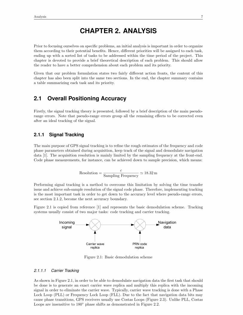
Figure 2.1 is copied from reference [1] and represents the basic demodulation scheme. Trackingsystems usually consist of two major tasks: code tracking and carrier tracking.
Incoming
signal
Navigation
data
Carrier wave replica
PRN code replica
Figure 2.1: Basic demodulation scheme
2.1.1.1 Carrier Tracking
As shown in Figure 2.1, in order to be able to demodulate navigation data the first task that shouldbe done is to generate an exact carrier wave replica and multiply this replica with the incomingsignal in order to eliminate the carrier wave. Typically, carrier wave tracking is done with a PhaseLock Loop (PLL) or Frequency Lock Loop (FLL). Due to the fact that navigation data bits maycause phase transitions, GPS receivers usually use Costas Loops (Figure 2.3). Unlike PLL, CostasLoops are insensitive to 180◦ phase shifts as demonstrated in Figure 2.2.
8 Enhancement Study of GPS Snapshot Techniques
I
Q
φ =0I
Q
φφ
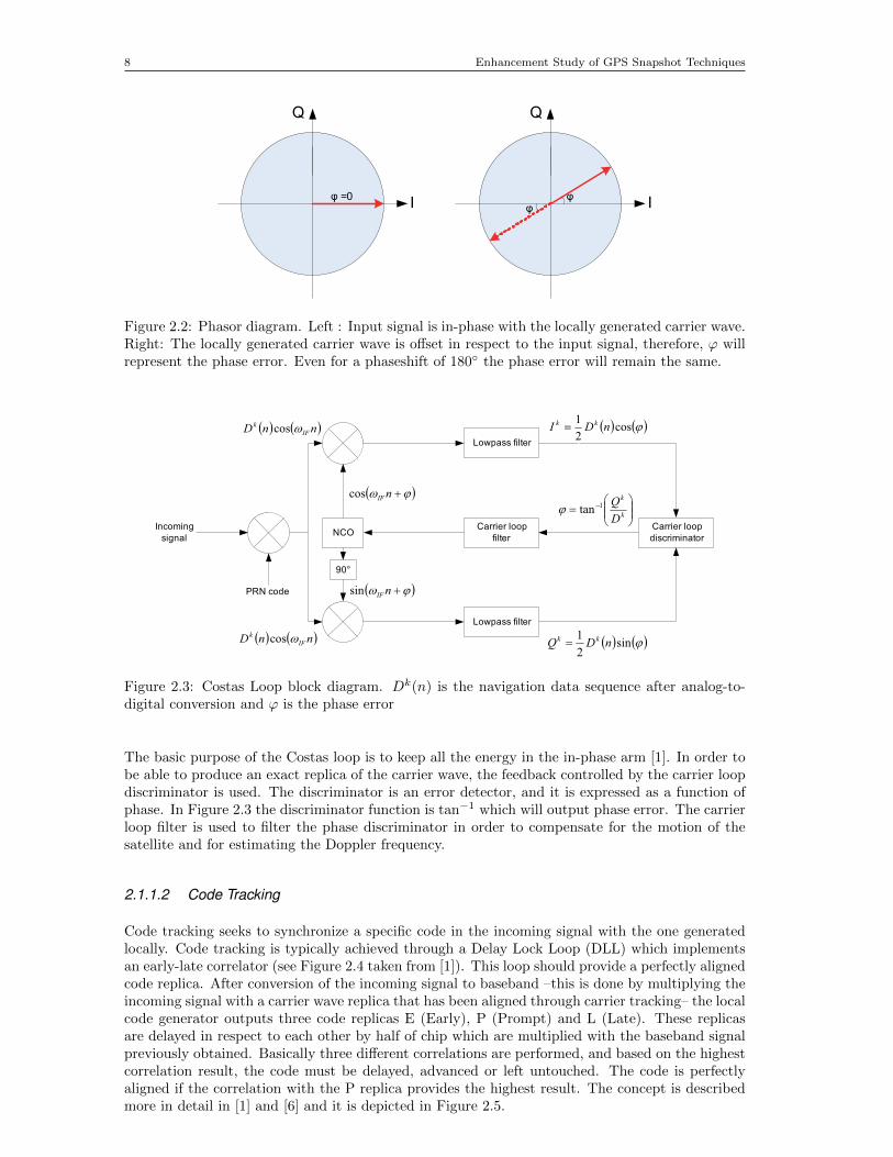
Figure 2.2: Phasor diagram. Left : Input signal is in-phase with the locally generated carrier wave.Right: The locally generated carrier wave is offset in respect to the input signal, therefore, ϕ willrepresent the phase error. Even for a phaseshift of 180◦ the phase error will remain the same.
Incoming
signal
PRN code
( ) ( )nnD IF
k ωcos
( ) ( )nnD IF
k ωcos
Lowpass filter
Lowpass filter
Carrier loop
discriminator
Carrier loop
filterNCO
90°
( )ϕω +nIFcos
( )ϕω +nIFsin
( ) ( )ϕcos2
1nDI kk =
( ) ( )ϕsin2
1nDQ kk =
= −
k
k
D
Q1tanϕ
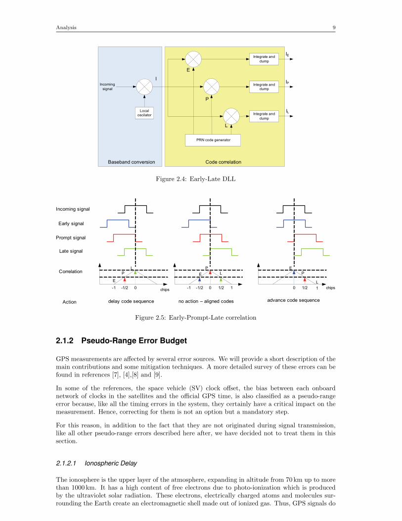
Figure 2.3: Costas Loop block diagram. Dk(n) is the navigation data sequence after analog-to-digital conversion and ϕ is the phase error
The basic purpose of the Costas loop is to keep all the energy in the in-phase arm [1]. In order tobe able to produce an exact replica of the carrier wave, the feedback controlled by the carrier loopdiscriminator is used. The discriminator is an error detector, and it is expressed as a function ofphase. In Figure 2.3 the discriminator function is tan−1 which will output phase error. The carrierloop filter is used to filter the phase discriminator in order to compensate for the motion of thesatellite and for estimating the Doppler frequency.
2.1.1.2 Code Tracking
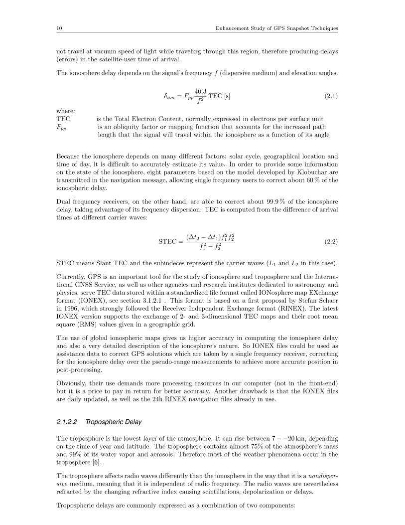
Code tracking seeks to synchronize a specific code in the incoming signal with the one generatedlocally. Code tracking is typically achieved through a Delay Lock Loop (DLL) which implementsan early-late correlator (see Figure 2.4 taken from [1]). This loop should provide a perfectly alignedcode replica. After conversion of the incoming signal to baseband –this is done by multiplying theincoming signal with a carrier wave replica that has been aligned through carrier tracking– the localcode generator outputs three code replicas E (Early), P (Prompt) and L (Late). These replicasare delayed in respect to each other by half of chip which are multiplied with the baseband signalpreviously obtained. Basically three different correlations are performed, and based on the highestcorrelation result, the code must be delayed, advanced or left untouched. The code is perfectlyaligned if the correlation with the P replica provides the highest result. The concept is describedmore in detail in [1] and [6] and it is depicted in Figure 2.5.
Analysis 9
Incoming
signal
Integrate and
dump
Local oscilator
Integrate and dump
Integrate and
dump
PRN code generator
I
E
P
L
IE
IP
IL
Baseband conversion Code correlation
Figure 2.4: Early-Late DLL
Incoming signal
Early signal
Late signal
Prompt signal
Correlation
Action delay code sequence no action – aligned codes advance code sequence
E
E
E
P
P
P
L
L
L
-1 -10 0 0-1/2 -1/2 1/2 11/2 1chips chips
Figure 2.5: Early-Prompt-Late correlation
2.1.2 Pseudo-Range Error Budget
GPS measurements are affected by several error sources. We will provide a short description of themain contributions and some mitigation techniques. A more detailed survey of these errors can befound in references [7], [4],[8] and [9].
In some of the references, the space vehicle (SV) clock offset, the bias between each onboardnetwork of clocks in the satellites and the official GPS time, is also classified as a pseudo-rangeerror because, like all the timing errors in the system, they certainly have a critical impact on themeasurement. Hence, correcting for them is not an option but a mandatory step.
For this reason, in addition to the fact that they are not originated during signal transmission,like all other pseudo-range errors described here after, we have decided not to treat them in thissection.
2.1.2.1 Ionospheric Delay
The ionosphere is the upper layer of the atmosphere, expanding in altitude from 70 km up to morethan 1000 km. It has a high content of free electrons due to photo-ionization which is producedby the ultraviolet solar radiation. These electrons, electrically charged atoms and molecules sur-rounding the Earth create an electromagnetic shell made out of ionized gas. Thus, GPS signals do
10 Enhancement Study of GPS Snapshot Techniques
not travel at vacuum speed of light while traveling through this region, therefore producing delays(errors) in the satellite-user time of arrival.
The ionosphere delay depends on the signal’s frequency f (dispersive medium) and elevation angles.
δion = Fpp40.3
f2TEC [s] (2.1)
where:TEC is the Total Electron Content, normally expressed in electrons per surface unitFpp is an obliquity factor or mapping function that accounts for the increased path
length that the signal will travel within the ionosphere as a function of its angle
Because the ionosphere depends on many different factors: solar cycle, geographical location andtime of day, it is difficult to accurately estimate its value. In order to provide some informationon the state of the ionosphere, eight parameters based on the model developed by Klobuchar aretransmitted in the navigation message, allowing single frequency users to correct about 60 % of theionospheric delay.
Dual frequency receivers, on the other hand, are able to correct about 99.9 % of the ionospheredelay, taking advantage of its frequency dispersion. TEC is computed from the difference of arrivaltimes at different carrier waves:
STEC =(∆t2 −∆t1)f21 f
22
f21 − f22(2.2)
STEC means Slant TEC and the subindeces represent the carrier waves (L1 and L2 in this case).
Currently, GPS is an important tool for the study of ionosphere and troposphere and the Interna-tional GNSS Service, as well as other agencies and research institutes dedicated to astronomy andphysics, serve TEC data stored within a standardized file format called IONosphere map EXchangeformat (IONEX), see section 3.1.2.1 . This format is based on a first proposal by Stefan Schaerin 1996, which strongly followed the Receiver Independent Exchange format (RINEX). The latestIONEX version supports the exchange of 2- and 3-dimensional TEC maps and their root meansquare (RMS) values given in a geographic grid.
The use of global ionospheric maps gives us higher accuracy in computing the ionosphere delayand also a very detailed description of the ionosphere’s nature. So IONEX files could be used asassistance data to correct GPS solutions which are taken by a single frequency receiver, correctingfor the ionosphere delay over the pseudo-range measurements to achieve more accurate position inpost-processing.
Obviously, their use demands more processing resources in our computer (not in the front-end)but it is a price to pay in return for better accuracy. Another drawback is that the IONEX filesare daily updated, as well as the 24h RINEX navigation files already in use.
2.1.2.2 Tropospheric Delay
The troposphere is the lowest layer of the atmosphere. It can rise between 7−−20 km, dependingon the time of year and latitude. The troposphere contains almost 75% of the atmosphere’s massand 99% of its water vapor and aerosols. Therefore most of the weather phenomena occur in thetroposphere [6].
The troposphere affects radio waves differently than the ionosphere in the way that it is a nondisper-sive medium, meaning that it is independent of radio frequency. The radio waves are neverthelessrefracted by the changing refractive index causing scintillations, depolarization or delays.
Tropospheric delays are commonly expressed as a combination of two components:
Analysis 11
• the “wet” component, water vapors, is usually around 10% of the total effect
• the “dry” component, oxygen and nitrogen in hydrostatic equilibrium, is the rest of 90%
Due to its continuous variation and unpredictability the “wet” component is the most difficult tomitigate.
Techniques of troposphere error mitigation include using Differential GPS (DGPS), solving fortropospheric delay based on elevation angle values and tropospheric modeling. The latter one willbe described in more detail in Section 3.1.2.2 .
2.1.2.3 Relativistic Errors
The word relativity evokes two kind of different errors in GPS systems: on one side, the “SagnacEffect” and, on the other side, the “General Relativity” encompassing the theories of AlbertEinstein.
Concerning “Sagnac Effect”, physical laws hold in all inertial frames. One has to take into accountthat the GPS system uses two different coordinates systems: Earth-Centered, Earth-Fixed (ECEF)and ECI (Earth Center Inertial). In this sense, the user shall take into account the Earth rotationcorrections during time of flight of the signal.
In respect to “General Relativity”, one has to consider that the GPS system relies on clocks inorbit, flying at high speeds and in different gravitational planes relative to Earth’s surface. Thespace-time curvature due to the Earth’s mass is less than it is at the Earth’s surface. Therefore,clocks closer to a massive object will seem to tick slower than those located further away. Luckily,scientists counteracted this effect by slowing down the frequency of the onboard atomic clocks sothat, once they were in orbit, the clocks would appear to tick at the correct rate as compared tothe reference clocks in the ground stations. However, the user still needs to correct for a smallerpart of the problem, and that is a component depending on the high speeds of the satellites. Themathematical equation for this correction can be found in [3]:
δrel = Fe√a sin(Ek) (2.3)
e is the eccentricity.a is the semi-major axis.Ek is the eccentric Anomaly.
and the constant F =−2√µc2 = −4.442807633 · 10−10.
This last left-over correction is optional and is the only one we will refer to while below talkingabout relativistic error.
2.1.2.4 Total Group Delay
The Total Group Delay (TGD) is a term provided by the ground segment that mainly accountsfor the instrumental delays of the satellites. Specifically, it is the delay suffered by the signal in thecircuitry of the satellite: between the creation instant and its transmission through the antenna.Each satellite has a different one and it is transmitted to the user in the navigation message.
This would lead to think that a similar parameter has to be taken into account for the delaysuffered on the receiver. Nevertheless, such delay is constant for all signals so it is canceled out orabsorbed in the navigation equations by the offset of the receiver clock.

12 Enhancement Study of GPS Snapshot Techniques
2.1.2.5 Multipath Errors
Usually, the receiver also acquires signals which are not only the direct line-of-sight but somereplicas that have been bounced by one or more obstacles. Therefore they are delayed in time, phaseshifted, and attenuated. However, their contribution may distort the spectrum of the incomingsignal, biasing the measurements from the correlators.
Multipath is the ultimate accuracy limiting phenomenon in Differential GPS techniques. Nowadaysthere are several techniques used to mitigate or minimize the multipath effects. These techniquesmay include: using multiple antenna groundplanes, using phase observations, averaging measure-ments over 24 hours, or implementing a receiver design with multiple correlators, or very narrowcorrelation functions.
All these techniques require hardware modifications that will only pay off for expensive professionalequipment but not for a mass market front-end. Thus, the only remaining choice is modeling whichis rather complicated in a dynamic scenario like our case-study. For this reason we have rejectedto apply any multipath corrections.
2.2 Assistance Data
By assisted data we understand all data provided through an external source rather than the GPSsignal itself. In this context, we would like to formally break down assistance data into two maincategories:
2.2.1 Mandatory Assistance Data
This refers to all required data that must be provided to the algorithm in order to obtain position-ing.
• Time: Coarse-time algorithm requires, as its name suggests, a time guess. As demonstratedin [5], this variable shall not be biased by more than 90 s. It shall be provided as Timeof Week, second within the current GPS week, format. Such value was obtained from theOperating System metadata of the snapshot file and manually input to the system.
• Apriori user coordinates: A rough fix of the user location is also required by the coarse-time algorithm. The coordinates shall not be biased by more than 150 km to the actualorigin, as demonstrated in [5]. Initially, these were manually introduced by the user. Analgorithm based on Doppler measurements after acquisition stage may be a solution allowingthe receiver to auto-assist itself with such information.
• Ephemeris: An accurate knowledge about satellite trajectories is necessary in order to com-pute its position at any given time, this being the basis of the trilateration concept. Ephemerisare formed by the almanac with the fundamental Keplerian parameters plus further temporalcorrections. Because the navigation message is not decoded by the receiver, a RINEX filecontaining them was manually downloaded and imported into the system by using our ownparsing function, called “loadrinexn.m”.
2.2.2 Supplementary Assistance Data
While addressing the issue of improving position accuracy we may need to access additional data.IONEX files presented in the previous section fall inside this category.
Analysis 13
2.3 Summary
By applying tracking algorithms we should be able to obtain more accurate values for code phaseand carrier frequency. This should lead us to get more accurate positioning results. While im-plementing tracking algorithms for GPS snapshots we have to keep in mind the short length ofthe snapshot because this may cause convergence failure, therefore we have to find alternativealgorithms.
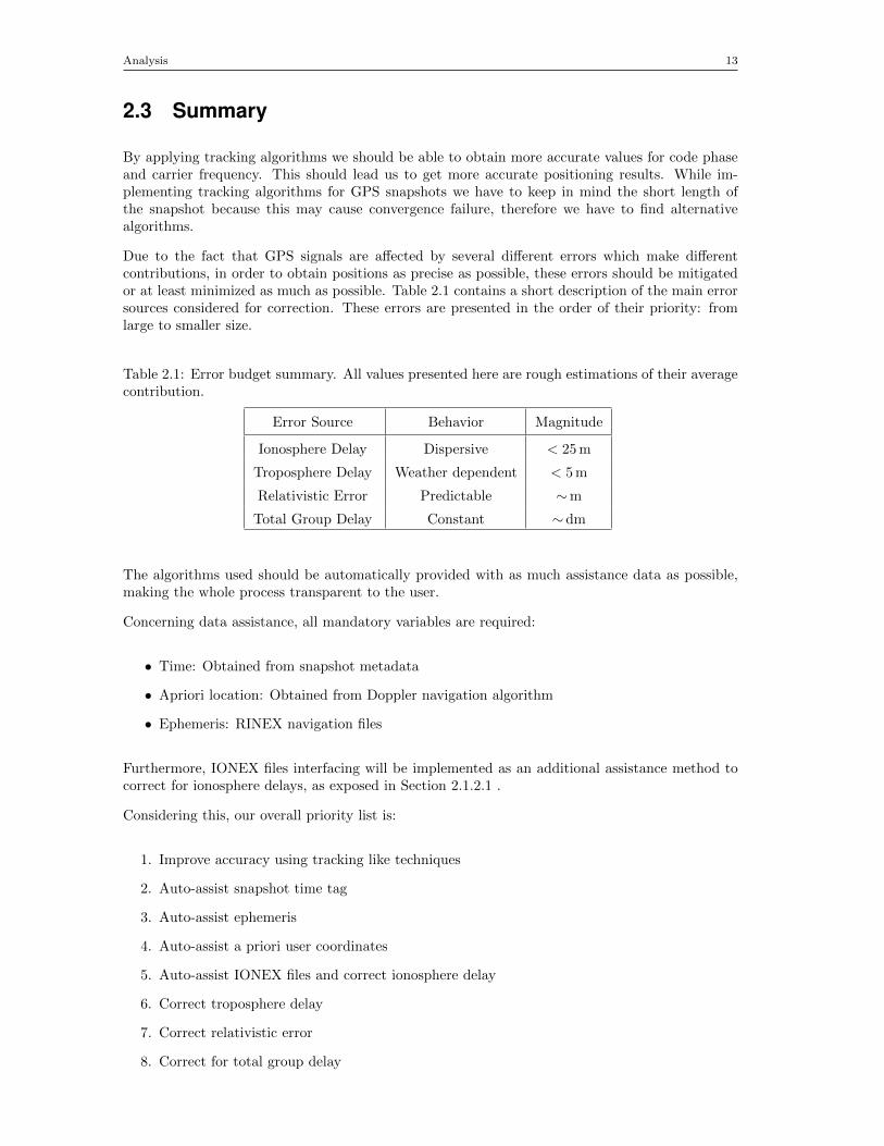
Due to the fact that GPS signals are affected by several different errors which make differentcontributions, in order to obtain positions as precise as possible, these errors should be mitigatedor at least minimized as much as possible. Table 2.1 contains a short description of the main errorsources considered for correction. These errors are presented in the order of their priority: fromlarge to smaller size.
Table 2.1: Error budget summary. All values presented here are rough estimations of their averagecontribution.
Error Source Behavior Magnitude
Ionosphere Delay Dispersive < 25 m
Troposphere Delay Weather dependent < 5 m
Relativistic Error Predictable ∼m
Total Group Delay Constant ∼dm
The algorithms used should be automatically provided with as much assistance data as possible,making the whole process transparent to the user.
Concerning data assistance, all mandatory variables are required:
• Time: Obtained from snapshot metadata
• Apriori location: Obtained from Doppler navigation algorithm
• Ephemeris: RINEX navigation files
Furthermore, IONEX files interfacing will be implemented as an additional assistance method tocorrect for ionosphere delays, as exposed in Section 2.1.2.1 .
Considering this, our overall priority list is:
1. Improve accuracy using tracking like techniques
2. Auto-assist snapshot time tag
3. Auto-assist ephemeris
4. Auto-assist a priori user coordinates
5. Auto-assist IONEX files and correct ionosphere delay
6. Correct troposphere delay
7. Correct relativistic error
8. Correct for total group delay

14 Enhancement Study of GPS Snapshot Techniques
Development 15
CHAPTER 3. DEVELOPMENT
This chapter goes deeper into the concepts identified in Section 2. A summary of the main high-lights will be, again, presented right before the experimental results.
3.1 Improving Accuracy
In this first section of the Development chapter we will detail how signal tracking is performed.After, a description of the pseudo-range corrections applied will follow. This will include thecorrection of the ionosphere delay using TEC information from IONEX, troposphere delay correc-tion through modeling and, lastly, performing weighted least-squares solutions using User RangeAccuracy (URA) and other weighting criteria.
3.1.1 Signal Tracking
This subsection extends the reasoning behind our decision to apply tracking algorithms in orderto improve position accuracy. The different ideas and concepts which have been implemented willbe presented.
We decided to apply tracking algorithms in order to improve the position results by refining theacquisition results. Due to the fact that we are dealing with short snapshot cuts (11 ms) we arenot dealing with traditional tracking. In order to generate pseudo-range measurements, traditionaltracking implies continuously generating a replica code in the receiver, perform correlation withthe incoming signal and, afterwards, decoding the navigation message from the GPS satellites. Inthe present project, due to short integration time, tracking convergence seemed difficult to obtain.Therefore we just want to correct the values obtained from acquisition, concentrating on the codephase. As a reminder, code phase is an independent time parameter of the PRN code, expressedin chips —portion of PRN waveform over the minimal time interval between code transitions [4]—which actually indicates where in the incoming signal the code corresponding to a certain PRNstarts. As previously stated our main purpose was to correct the code phase values. The startingpoint for our algorithms was the tracking function (tracking.m) from the softGPS project, whichis an attachment of the reference book [10].
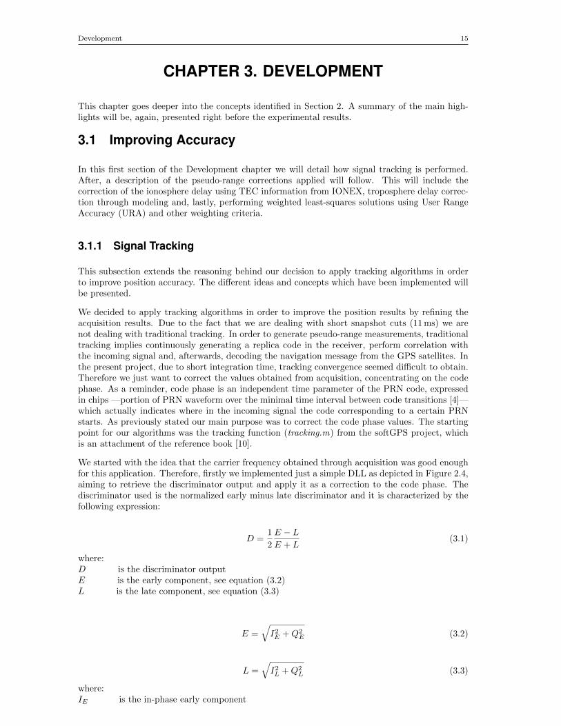
We started with the idea that the carrier frequency obtained through acquisition was good enoughfor this application. Therefore, firstly we implemented just a simple DLL as depicted in Figure 2.4,aiming to retrieve the discriminator output and apply it as a correction to the code phase. Thediscriminator used is the normalized early minus late discriminator and it is characterized by thefollowing expression:
D =1
2
E − LE + L
(3.1)
where:D is the discriminator outputE is the early component, see equation (3.2)L is the late component, see equation (3.3)
E =√I2E +Q2
E (3.2)
L =√I2L +Q2
L (3.3)
where:IE is the in-phase early component
16 Enhancement Study of GPS Snapshot Techniques
QE is the quadrature early componentIL is the in-phase late componentQL is the quadrature late component
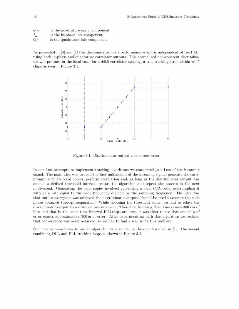
As presented in [4] and [1] this discriminator has a performance which is independent of the PLL,using both in-phase and quadrature correlator outputs. This normalized non-coherent discrimina-tor will produce in the ideal case, for a ±0.5 correlator spacing, a true tracking error within ±0.5chips as seen in Figure 3.1.
Figure 3.1: Discriminator output versus code error
In our first attempts to implement tracking algorithms we considered just 1 ms of the incomingsignal. The main idea was to read the first millisecond of the incoming signal, generate the early,prompt and late local copies, perform correlation and, as long as the discriminator output wasoutside a defined threshold interval, restart the algorithm and repeat the process in the nextmillisecond. Generating the local copies involved generating a local C/A code, oversampling itwith at a rate equal to the code frequency divided by the sampling frequency. The idea wasthat until convergence was achieved the discriminator outputs should be used to correct the codephase obtained through acquisition. While choosing the threshold value, we had to relate thediscriminator output to a distance measurement. Therefore, knowing that 1 ms causes 300 km ofbias and that in the same time interval 1024 chips are sent, it was clear to see that one chip oferror causes approximately 300 m of error. After experimenting with this algorithm we realizedthat convergence was never achieved, so we had to find a way to fix this problem.
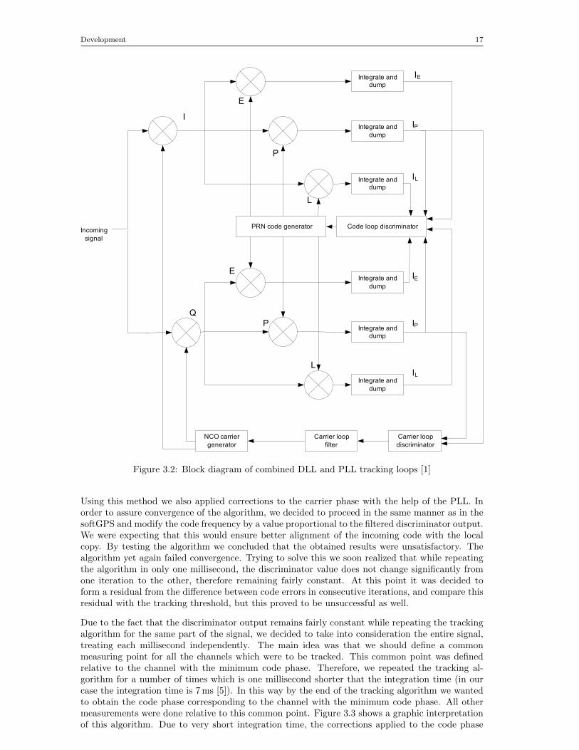
Our next approach was to use an algorithm very similar to the one described in [1]. This meantcombining DLL and PLL tracking loops as shown in Figure 3.2.
Development 17
Incoming
signal
Integrate and dump
Integrate and
dump
Integrate and dump
PRN code generator
I
E
P
L
IE
IP
IL
Integrate and
dump
Integrate and dump
Integrate and
dump
Q
E
P
L
Code loop discriminator
IP
IL
IE
Carrier loop
discriminator
Carrier loop
filter
NCO carrier
generator
Figure 3.2: Block diagram of combined DLL and PLL tracking loops [1]
Using this method we also applied corrections to the carrier phase with the help of the PLL. Inorder to assure convergence of the algorithm, we decided to proceed in the same manner as in thesoftGPS and modify the code frequency by a value proportional to the filtered discriminator output.We were expecting that this would ensure better alignment of the incoming code with the localcopy. By testing the algorithm we concluded that the obtained results were unsatisfactory. Thealgorithm yet again failed convergence. Trying to solve this we soon realized that while repeatingthe algorithm in only one millisecond, the discriminator value does not change significantly fromone iteration to the other, therefore remaining fairly constant. At this point it was decided toform a residual from the difference between code errors in consecutive iterations, and compare thisresidual with the tracking threshold, but this proved to be unsuccessful as well.
Due to the fact that the discriminator output remains fairly constant while repeating the trackingalgorithm for the same part of the signal, we decided to take into consideration the entire signal,treating each millisecond independently. The main idea was that we should define a commonmeasuring point for all the channels which were to be tracked. This common point was definedrelative to the channel with the minimum code phase. Therefore, we repeated the tracking al-gorithm for a number of times which is one millisecond shorter that the integration time (in ourcase the integration time is 7 ms [5]). In this way by the end of the tracking algorithm we wantedto obtain the code phase corresponding to the channel with the minimum code phase. All othermeasurements were done relative to this common point. Figure 3.3 shows a graphic interpretationof this algorithm. Due to very short integration time, the corrections applied to the code phase
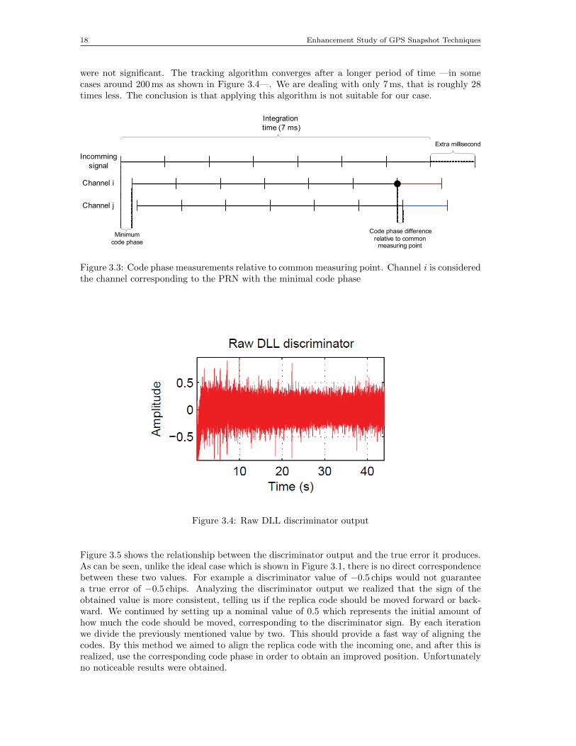
18 Enhancement Study of GPS Snapshot Techniques
were not significant. The tracking algorithm converges after a longer period of time —in somecases around 200 ms as shown in Figure 3.4—. We are dealing with only 7 ms, that is roughly 28times less. The conclusion is that applying this algorithm is not suitable for our case.
Integration
time (7 ms)
Minimum
code phase
Code phase difference
relative to common measuring point
Extra millisecond
Incomming
signal
Channel i
Channel j
Figure 3.3: Code phase measurements relative to common measuring point. Channel i is consideredthe channel corresponding to the PRN with the minimal code phase
Figure 3.4: Raw DLL discriminator output
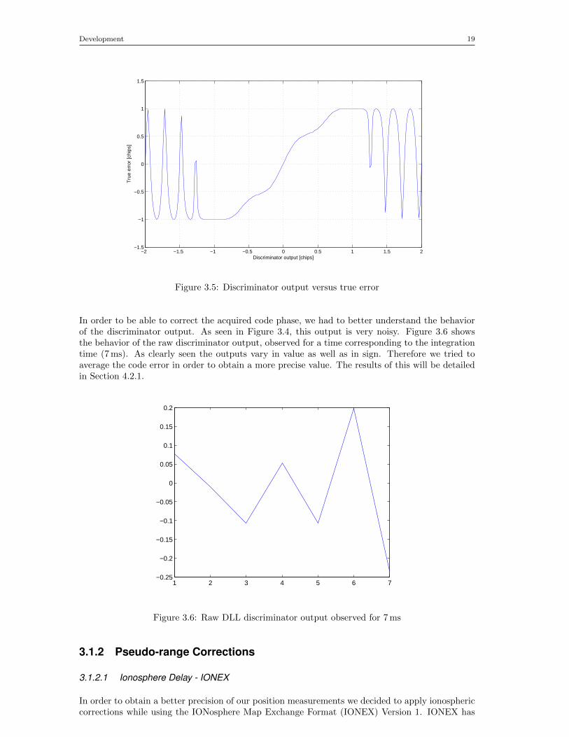
Figure 3.5 shows the relationship between the discriminator output and the true error it produces.As can be seen, unlike the ideal case which is shown in Figure 3.1, there is no direct correspondencebetween these two values. For example a discriminator value of −0.5 chips would not guaranteea true error of −0.5 chips. Analyzing the discriminator output we realized that the sign of theobtained value is more consistent, telling us if the replica code should be moved forward or back-ward. We continued by setting up a nominal value of 0.5 which represents the initial amount ofhow much the code should be moved, corresponding to the discriminator sign. By each iterationwe divide the previously mentioned value by two. This should provide a fast way of aligning thecodes. By this method we aimed to align the replica code with the incoming one, and after this isrealized, use the corresponding code phase in order to obtain an improved position. Unfortunatelyno noticeable results were obtained.
Development 19
−2 −1.5 −1 −0.5 0 0.5 1 1.5 2−1.5
−1
−0.5
0
0.5
1
1.5
Discriminator output [chips]
Tru
e er
ror
[chi
ps]
Figure 3.5: Discriminator output versus true error
In order to be able to correct the acquired code phase, we had to better understand the behaviorof the discriminator output. As seen in Figure 3.4, this output is very noisy. Figure 3.6 showsthe behavior of the raw discriminator output, observed for a time corresponding to the integrationtime (7 ms). As clearly seen the outputs vary in value as well as in sign. Therefore we tried toaverage the code error in order to obtain a more precise value. The results of this will be detailedin Section 4.2.1.
1 2 3 4 5 6 7−0.25
−0.2
−0.15
−0.1
−0.05
0
0.05
0.1
0.15
0.2
Figure 3.6: Raw DLL discriminator output observed for 7 ms
3.1.2 Pseudo-range Corrections
3.1.2.1 Ionosphere Delay - IONEX
In order to obtain a better precision of our position measurements we decided to apply ionosphericcorrections while using the IONosphere Map Exchange Format (IONEX) Version 1. IONEX has
20 Enhancement Study of GPS Snapshot Techniques
been created in order to satisfy the GPS world’s need for a common data format which enables theexchange, comparison, or combination of Total Electron Content (TEC) maps [11]. This format,which is described more in detail in [11], supports 2-dimensional and 3-dimensional TEC maps andTEC Root Mean Square (RMS) values given in a geographic grid formed by constant incrementsin latitude and longitude, for a specific epoch . However, the IONEX file is also able to supportdifferent maps which correspond to different epochs. A 24 hours IONEX file can support a numberof 13 TEC maps, therefore describing the ionosphere at an approximate interval of 1 hour and51 minutes. The IONEX data files are created by combining measurements from a large numberof dual-frequency receivers which are spread around the world in specific locations, combiningmeasurements obtained from the International GPS Service for Geodynamics (IGS) as well asother external processing centers.
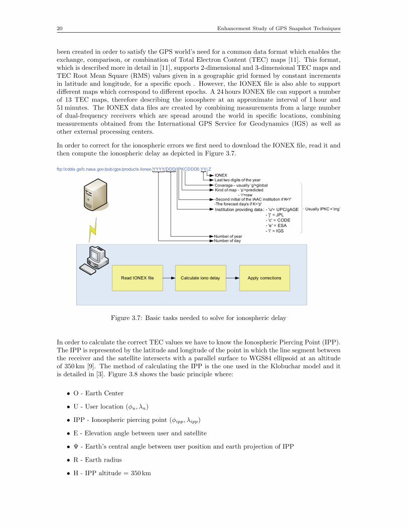
In order to correct for the ionospheric errors we first need to download the IONEX file, read it andthen compute the ionospheric delay as depicted in Figure 3.7.
ftp://cddis .gsfc.nasa.gov/pub/gps/products /ionex/YYYY/DDD/IPKCDDD0.YYi.Z
IONEXLast two digits of the year
Covarage – usually ‘g’=globalKind of map - ‘p’=predicted
- ‘r’=raw -Second initial of the IAAC institution if K='r'-The forecast day/s if K='p'
Institution providing data : - 'u'= UPC/gAGE
- 'j' = JPL
- 'c' = CODE
- 'e' = ESA
- 'i' = IGS
Number of yearNumber of day
Usually IPKC =’irrg’
Read IONEX file Calculate iono delay Apply corrections
Figure 3.7: Basic tasks needed to solve for ionospheric delay
In order to calculate the correct TEC values we have to know the Ionospheric Piercing Point (IPP).The IPP is represented by the latitude and longitude of the point in which the line segment betweenthe receiver and the satellite intersects with a parallel surface to WGS84 ellipsoid at an altitudeof 350 km [9]. The method of calculating the IPP is the one used in the Klobuchar model and itis detailed in [3]. Figure 3.8 shows the basic principle where:
• O - Earth Center
• U - User location (φu, λu)
• IPP - Ionospheric piercing point (φipp, λipp)
• E - Elevation angle between user and satellite
• Ψ - Earth’s central angle between user position and earth projection of IPP
• R - Earth radius
• H - IPP altitude = 350 km
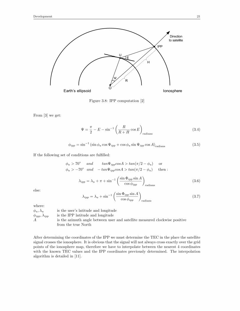
Development 21
Earth’s ellipsoid IonosphereO
U
IPP
E
Ψ
Direction
to satellite
R
H
Figure 3.8: IPP computation [2]
From [3] we get:
Ψ =π
2− E − sin−1
(R
R+HcosE
)radians
(3.4)
φipp = sin−1 (sinφu cos Ψipp + cosφu sin Ψipp cosA)radians (3.5)
If the following set of conditions are fulfilled:
φu > 70◦ and tanΨippcosA > tan(π/2− φu) or
φu > −70◦ and − tanΨippcosA > tan(π/2− φu) then :
λipp = λu + π + sin−1(
sin Φipp sinA
cosφipp
)radians
(3.6)
else:
λipp = λu + sin−1(
sin Φipp sinA
cosφipp
)radians
(3.7)
where:φu, λu is the user’s latitude and longitudeφipp, λipp is the IPP latitude and longitudeA is the azimuth angle between user and satellite measured clockwise positive
from the true North
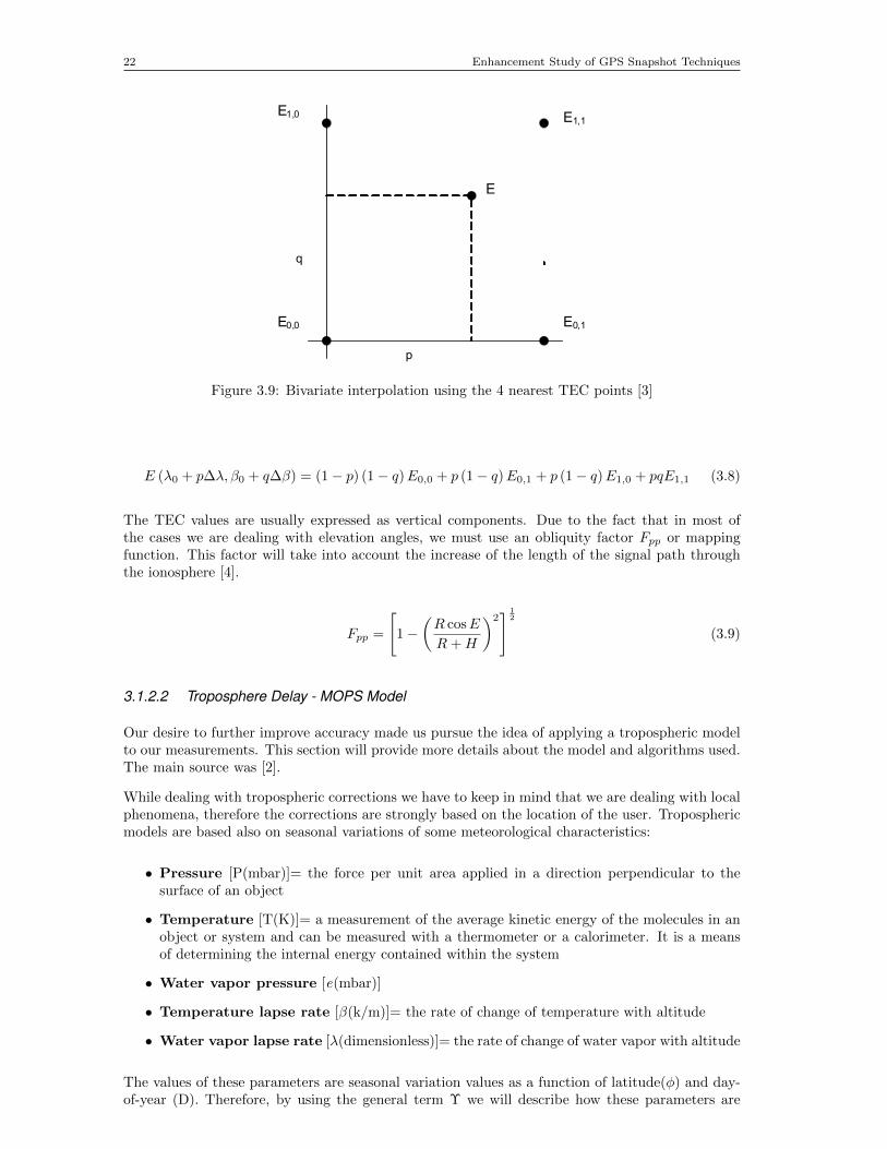
After determining the coordinates of the IPP we must determine the TEC in the place the satellitesignal crosses the ionosphere. It is obvious that the signal will not always cross exactly over the gridpoints of the ionosphere map, therefore we have to interpolate between the nearest 4 coordinateswith the known TEC values and the IPP coordinates previously determined. The interpolationalgorithm is detailed in [11].
22 Enhancement Study of GPS Snapshot Techniques
E1,0 E1,1
E0,0 E0,1
E
q
p
Figure 3.9: Bivariate interpolation using the 4 nearest TEC points [3]
E (λ0 + p∆λ, β0 + q∆β) = (1− p) (1− q)E0,0 + p (1− q)E0,1 + p (1− q)E1,0 + pqE1,1 (3.8)
The TEC values are usually expressed as vertical components. Due to the fact that in most ofthe cases we are dealing with elevation angles, we must use an obliquity factor Fpp or mappingfunction. This factor will take into account the increase of the length of the signal path throughthe ionosphere [4].
Fpp =
[1−
(R cosE
R+H
)2] 1
2
(3.9)
3.1.2.2 Troposphere Delay - MOPS Model
Our desire to further improve accuracy made us pursue the idea of applying a tropospheric modelto our measurements. This section will provide more details about the model and algorithms used.The main source was [2].
While dealing with tropospheric corrections we have to keep in mind that we are dealing with localphenomena, therefore the corrections are strongly based on the location of the user. Troposphericmodels are based also on seasonal variations of some meteorological characteristics:
• Pressure [P(mbar)]= the force per unit area applied in a direction perpendicular to thesurface of an object
• Temperature [T(K)]= a measurement of the average kinetic energy of the molecules in anobject or system and can be measured with a thermometer or a calorimeter. It is a meansof determining the internal energy contained within the system
• Water vapor pressure [e(mbar)]
• Temperature lapse rate [β(k/m)]= the rate of change of temperature with altitude
• Water vapor lapse rate [λ(dimensionless)]= the rate of change of water vapor with altitude
The values of these parameters are seasonal variation values as a function of latitude(φ) and day-of-year (D). Therefore, by using the general term Υ we will describe how these parameters are
Development 23
obtained, as detailed in [2]:
Υ(φ,D) = Υ0(φ)−∆Υ(φ) cos
(2π(D −Dmin)
365.25
)(3.10)
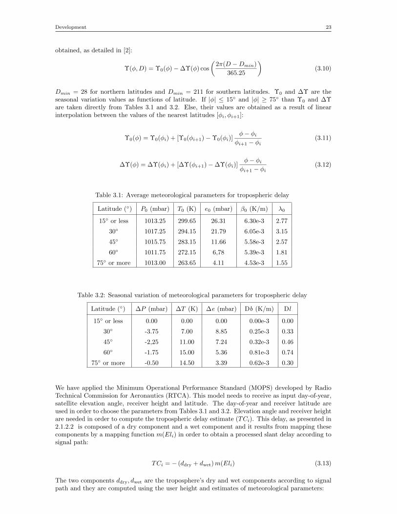
Dmin = 28 for northern latitudes and Dmin = 211 for southern latitudes. Υ0 and ∆Υ are theseasonal variation values as functions of latitude. If |φ| ≤ 15◦ and |φ| ≥ 75◦ than Υ0 and ∆Υare taken directly from Tables 3.1 and 3.2. Else, their values are obtained as a result of linearinterpolation between the values of the nearest latitudes [φi, φi+1]:
Υ0(φ) = Υ0(φi) + [Υ0(φi+1)−Υ0(φi)]φ− φi
φi+1 − φi(3.11)
∆Υ(φ) = ∆Υ(φi) + [∆Υ(φi+1)−∆Υ(φi)]φ− φi
φi+1 − φi(3.12)
Table 3.1: Average meteorological parameters for tropospheric delay
Latitude (◦) P0 (mbar) T0 (K) e0 (mbar) β0 (K/m) λ0
15◦ or less 1013.25 299.65 26.31 6.30e-3 2.77
30◦ 1017.25 294.15 21.79 6.05e-3 3.15
45◦ 1015.75 283.15 11.66 5.58e-3 2.57
60◦ 1011.75 272.15 6,78 5.39e-3 1.81
75◦ or more 1013.00 263.65 4.11 4.53e-3 1.55
Table 3.2: Seasonal variation of meteorological parameters for tropospheric delay
Latitude (◦) ∆P (mbar) ∆T (K) ∆e (mbar) Db (K/m) Dl
15◦ or less 0.00 0.00 0.00 0.00e-3 0.00
30◦ -3.75 7.00 8.85 0.25e-3 0.33
45◦ -2,25 11.00 7.24 0.32e-3 0.46
60◦ -1.75 15.00 5.36 0.81e-3 0.74
75◦ or more -0.50 14.50 3.39 0.62e-3 0.30
We have applied the Minimum Operational Performance Standard (MOPS) developed by RadioTechnical Commission for Aeronautics (RTCA). This model needs to receive as input day-of-year,satellite elevation angle, receiver height and latitude. The day-of-year and receiver latitude areused in order to choose the parameters from Tables 3.1 and 3.2. Elevation angle and receiver heightare needed in order to compute the tropospheric delay estimate (TCi). This delay, as presented in2.1.2.2 is composed of a dry component and a wet component and it results from mapping thesecomponents by a mapping function m(Eli) in order to obtain a processed slant delay according tosignal path:
TCi = − (ddry + dwet)m(Eli) (3.13)
The two components ddry, dwet are the troposphere’s dry and wet components according to signalpath and they are computed using the user height and estimates of meteorological parameters:
24 Enhancement Study of GPS Snapshot Techniques
ddry = zdry
(1− βH
T
) gRdβ
(3.14)
dwet = zwet
(1− βH
T
) (λ+1)gRdβ
−1
(3.15)
where g= 9.80665m/s2, H is the receivers height above the mean sea level, Rd = 287.054 J/kg/Kand zdry and zwet are the dry and wet components at zenith:
zdry =10−6k1RdP
gm(3.16)
zwet =10−6k2Rde
[gm(λ+ 1)− βRd]T(3.17)
where k1 = 77.604 K/mbar, k2 = 382000 K2/mbar and gm = 9.784m/s2.
The only thing that is still needed in order to calculate the tropospheric delay is the mappingfunction, which is a function of satellite elevation angle, being valid only for elevation anglesgreater that 5◦:
m(Eli) =1.001√
0.002001 + sin2(Eli)(3.18)
3.1.3 Weighted Least Squares
Once all pseudo-range measurements have been obtained and corrected, it is time to formulatethe observation equations that will result in a fix. Summarizing, the observation equations form asystem based on a linearization of the distance vectors (pseudo-range measurement) between thesatellites and the user. Such a linear system can be summarized like:
δz = Hδx + ε (3.19)
where:H is a matrix of normalized geometric distances between user and satellitesδz = z− z is the vector of a-priori pseudo-range measurement residualsz is the vector of measured pseudo-rangesz is the vector of predicted geometric distancesε is the vector of measurement and linearization errors
δx =
δxδyδzδb
is the vector of updates to the a-priori state: x, y, z and b
Least Squares (LS) method is the traditional way to solve an over-determined system. The solutionis:
δx =(HTH
)−1HT δz (3.20)
However, Weighted Least Squares (WLS), is an algebraic function that extends LS assigning arelative degree of “trust” to each one of the equations improving our estimation according tothem. Thus, it allows us to refine the results taking into account additional information. Theweight matrix W will be used in computing least-squares solution for the position:
Development 25
δx =(HTWH
)−1HTWδz (3.21)
where W is a diagonal matrix:
W =
w1 0 . . . 00 w2 . . . 0...
. . ....
0 . . . 0 wi
(3.22)
wi is the weight corresponding to satellite i.
It is up to the user to introduce the weights. A possible option is to select a weight based on theelevation of the satellite in the sky, as described in PhD Thesis [12], the reasoning behind this reliesin the fact that code observations may deteriorate with decreasing satellite elevations, so their rootmean square errors are higher. In that study, it was found that such dependance could be easilymodeled through the following expression:
y = a0 + a1exp(−eli/el0) (3.23)
y is the root mean square error in the code observationsa0 and a1 are constants defining the offset and exponential gainel0 is an reference elevation angleeli is the elevation of satellite i in the skyAll elevation angles are expressed in degrees
The value of y could be used to define the weight:
wi =1
y2(3.24)
Some other common weighting criteria are described in the next paragraphs.
3.1.3.1 User Range Accuracy - URA
A usual option is to use the User Range Accuracy (URA) indicator as weight, described in [3].As defined in [3] the User Range Accuracy (URA) is in fact a statistical indicator of the rangingerrors which can be obtained with a specific satellite. URA can be obtained from the navigationmessage. URA indicators provide only information about the errors for which the Space andControl Segments are responsible. Therefore URA indexes do not contain any error informationcorresponding to the User Segment or to the transmission medium.
URA indeces therefore give information about space vehicle accuracy. They are contained in bits13 to 16 of the third word in the first subframe in the navigation message. As it is described morein detail in [1], the navigation data contains a frame of 1500 bits. This frame is divided into 5subframes, each 300 bits in length. Each of these subframes contain 10 30 bit words.
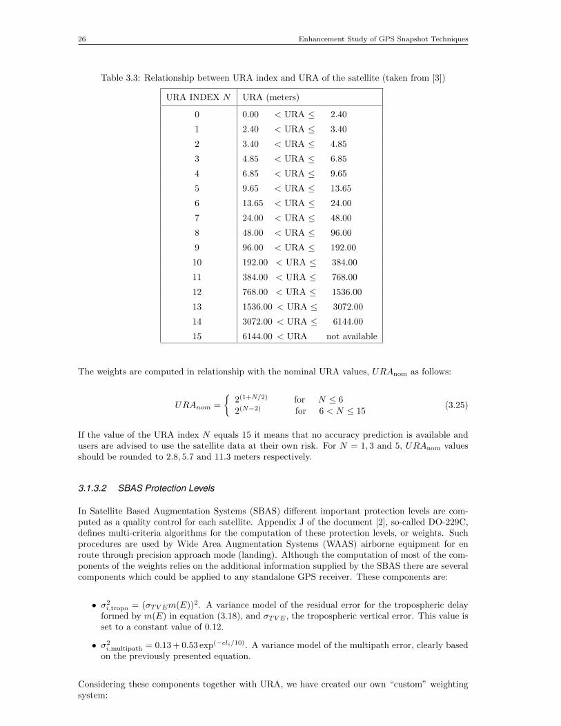
The URA index is an integer N ranging from 0 to 15 which is related with the range accuracy ofthe space vehicle as it is presented in Table 3.3.
26 Enhancement Study of GPS Snapshot Techniques
Table 3.3: Relationship between URA index and URA of the satellite (taken from [3])
URA INDEX N URA (meters)
0 0.00 < URA ≤ 2.40
1 2.40 < URA ≤ 3.40
2 3.40 < URA ≤ 4.85
3 4.85 < URA ≤ 6.85
4 6.85 < URA ≤ 9.65
5 9.65 < URA ≤ 13.65
6 13.65 < URA ≤ 24.00
7 24.00 < URA ≤ 48.00
8 48.00 < URA ≤ 96.00
9 96.00 < URA ≤ 192.00
10 192.00 < URA ≤ 384.00
11 384.00 < URA ≤ 768.00
12 768.00 < URA ≤ 1536.00
13 1536.00 < URA ≤ 3072.00
14 3072.00 < URA ≤ 6144.00
15 6144.00 < URA not available
The weights are computed in relationship with the nominal URA values, URAnom as follows:
URAnom =
{2(1+N/2) for N ≤ 62(N−2) for 6 < N ≤ 15
(3.25)
If the value of the URA index N equals 15 it means that no accuracy prediction is available andusers are advised to use the satellite data at their own risk. For N = 1, 3 and 5, URAnom valuesshould be rounded to 2.8, 5.7 and 11.3 meters respectively.
3.1.3.2 SBAS Protection Levels
In Satellite Based Augmentation Systems (SBAS) different important protection levels are com-puted as a quality control for each satellite. Appendix J of the document [2], so-called DO-229C,defines multi-criteria algorithms for the computation of these protection levels, or weights. Suchprocedures are used by Wide Area Augmentation Systems (WAAS) airborne equipment for enroute through precision approach mode (landing). Although the computation of most of the com-ponents of the weights relies on the additional information supplied by the SBAS there are severalcomponents which could be applied to any standalone GPS receiver. These components are:
• σ2i,tropo = (σTV Em(E))2. A variance model of the residual error for the tropospheric delay
formed by m(E) in equation (3.18), and σTV E , the tropospheric vertical error. This value isset to a constant value of 0.12.
• σ2i,multipath = 0.13 + 0.53 exp(−eli/10). A variance model of the multipath error, clearly based
on the previously presented equation.
Considering these components together with URA, we have created our own “custom” weightingsystem:
Development 27
σ2i = σ2
i,URA + σ2i,tropo + σ2
i,multipath (3.26)
3.2 Auto-Assistance
This section continues to describe the way assisted data is obtained, either from the Internet orthrough algebraic methods such as the Doppler positioning algorithm (assisting a priori coordi-nates) or the Time of Week algorithm (assisting a snapshot time to those snapshots not properlytime-tagged by the operating system) we have invented.
In order to have an application which can be used by any kind of user (not only dedicated toprofessionals) we want the user to have a minimum number of tasks to do in order to get positionsof his digital photographs. This is the reason why we wanted to provide our algorithms with moreassisted data.
3.2.1 Assisted Time
Our first report [5] about snapshot techniques, stated that the convergence strength towards awrong assisted time allows a bias of ±100 s. Therefore we assumed that the internal cameraclock could be re-synchronized with the Universal Time Coordinate (UTC) each time the camerais connected to a laptop, computer or, alternatively, coordinated with GPS Time (GPST) bydecoding the Time of Week (TOW) from time to time. Therefore, the camera shall be able toattach a time tag to each snapshot, which would be accurate enough to provide an initial time forthe positioning algorithms to converge. Ignoring the assumption that the camera has the means toassist time information, the front-end itself, in fact, does not provide any other data rather thanIF samples.
In our case, these samples are stored into a file under Windows OS (Operating System). In general,any file within an OS has different metadata (information about the information contained into thefile) or associated attributes describing its content. In Windows OS, for instance, regardless whichtype of file systems — New Technology File System (NTFS) or any File Allocation Table (FAT)version— is used, there are a minimum of metadata fields or details of a file: Name (string), Size(in Bytes), Type (typically indicated through the extension of the file and it associates the contentwith a program or application able to process it), Creation Time, Modification Time and AccessTime. All these time attributes are set using the internal CPU clock of the laptop/computer. Atthe same time, this clock uses to be automatically synchronized with a time server of its domain(network of computers) or another time server on the Internet. Therefore, unless the computer isisolated, all files are automatically time tagged during their creation at UTC.
Until now, time assistance has been manually performed by introducing creation time of the snap-shot file into the positioning algorithms. Along this project, we have programmed the automati-zation of this process as a new feature. To do so, a piece of C code, which uses standard Windowslibraries for this purpose, has been pre-compiled into a MEX-file (Matlab EXternal file) so thatthe function can be invoked from MATLAB’s workspace and retrieve the creation time from OSmetadata. As a result, this approximation relies on the correct time synchronization of the CPUclock.
However, in the event of a non-synchronized CPU clock, such procedure will not work. In theprevious project [5], there was a snapshot taken in Spain, identified as “S2C”, (a table with allsnapshots and their IDs is provided in appendix A. Many references to this table will be doneduring Section 3.2.1.1 ) that never provided satisfactory results. Although we suspected it couldbe due to a wrong time-tagging of the file, we had no means to demonstrate that, so we concludedclaiming that it might be due to some kind of hardware malfunction. This problem led us tothe creation of an algorithm able to estimate TW (Time of Week) of a snapshot. As a result,it was possible to obtain satisfactory results using the estimated time, hence demonstrating thatdivergence was caused by wrong time tagging due to CPU clock isolation instead of an error in our
28 Enhancement Study of GPS Snapshot Techniques
code. Next section describes the algorithm used to estimate TW of a snapshot.
3.2.1.1 TOW Estimation
This section describes an algorithm for estimating the time instant at which a given snapshot wastaken. Its inputs are date, ephemeris and location of the snapshot, as well as the snapshot itself.The output is a time estimate expressed as TW with an accuracy of few seconds.
Firstly, it is important to remark that this algorithm only works if the date and the user coordinatesare known. It might seem a nonsense to program an algorithm which requires user coordinates asan input, whereas this is typically our unknown, but, in our case, it was useful to recover TOW ofsnapshot “S2C”. This snapshot was taken in a computer running with a non-synchronized clockbecause, for safety reasons, it was isolated from any network. However, this problem lead to thecreation of this algorithm, which is, at least, interesting from a theoretical point of view.
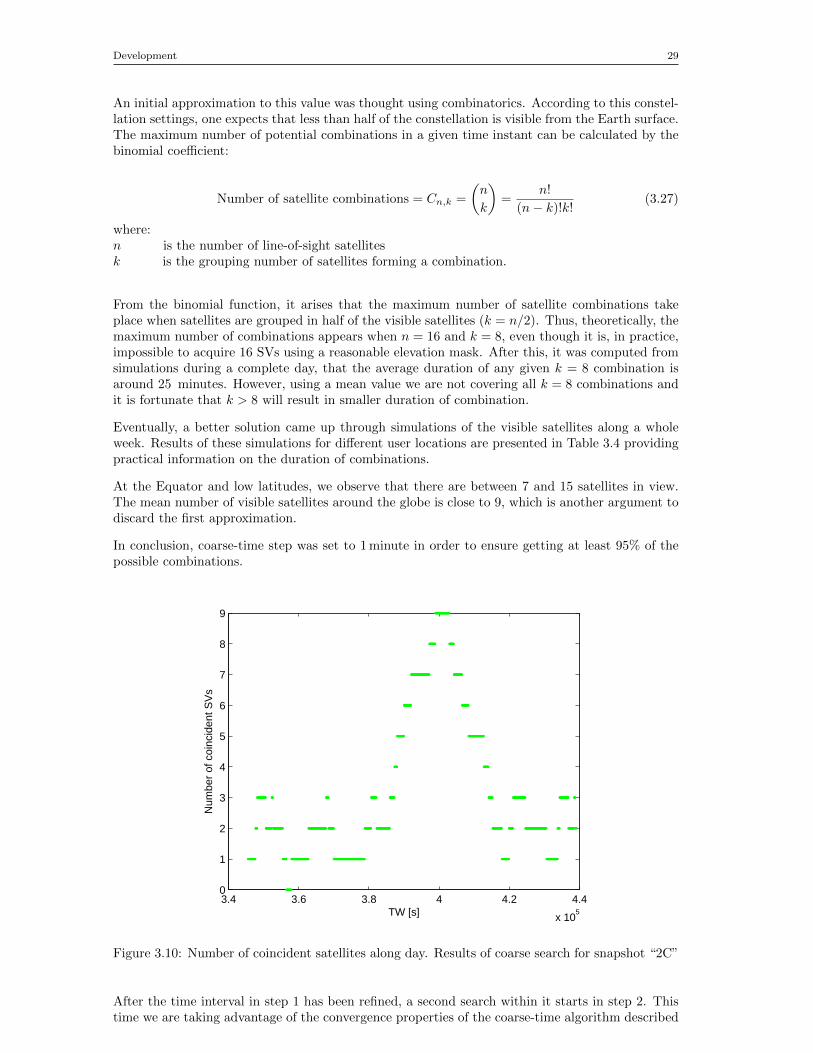
Basically the algorithm performs three steps:
1. Find the time interval where the acquired satellites best fit with line-of-sight interval.
2. Compute coarse-time algorithm within that time interval, ruling out those time instanceswhich are resulting in divergence or “big” distance residuals.
3. Find the residuals’ time trend-line and differentiate it in order to compute TOW wheredistance residual is minimum.
In step 2, “big” means a distance residual above 1 km between the position computed throughcoarse-time algorithm and the actual receiver position. In practice, step 1 and 2 are broken downinto two search routines: coarse and fine. Their only difference is the time step they use: whereasfine searches always use a 1 s time step, coarse time steps are set to optimize execution time of thefunction.
If our aim is to find the time interval where line-of-sight satellites best fit with acquired ones, weshall set up a coarse time step according to constellation architecture and dynamics. Thus, at thispoint, it is worth to refresh general characteristics of GPS orbits.
Currently, the GPS constellation is formed by 32 active satellites in 6 equally spaced orbital planes,each rotated 60 ◦ relative to the preceding plane . Satellites are not equally spaced within theorbital planes, and there are phase offsets between planes to achieve improved Geometric Dilutionof Precision (GDOP) characteristics of the constellation [4]. All orbital planes are inclined by 55 ◦.Concerning dynamics, the same satellites repeat to be at line-of-sight every sideral day for a staticobserver, so the period is half a sideral day. For further details on constellation design aiming forcontinuous whole-Earth coverage refer to [13]. As a result, in order to ensure at least 4 satellitesin the sky, the practical constraint for coverage of the GPS constellation was set to a minimum ofsixfold coverage above 5◦ minimum elevation angle [4].
Seeking for an optimum coarse time step, one shall consider that even if the algorithm is not fineenough to hit the exact satellite combination after acquisition, at least, it shall ensure to matchmost of them. Furthermore, note that acquisition might provide false alarms, acquire satelliteswhich are not in view, or miss some satellite(s) in line-of-sight. Thus, while maximizing thenumber of coincident satellites is important to drop the probability of repetition of any satellitecombination.
Roughly, the duration of any combination can take between 0 s and half of a sidereal day. Commonsense tells that the duration of a given satellite combination decreases inversely to the amount ofsatellites conforming it. In case we decided to set the coarse time step just considering this fact,in the event of 15 acquired satellites, the time step would have been so close to the fine one thatits purpose would have been ruined, giving rise to large execution times. Therefore, the logicaldecision is to select a time step according to the duration of most of the cases.
Development 29
An initial approximation to this value was thought using combinatorics. According to this constel-lation settings, one expects that less than half of the constellation is visible from the Earth surface.The maximum number of potential combinations in a given time instant can be calculated by thebinomial coefficient:
Number of satellite combinations = Cn,k =
(n
k
)=
n!
(n− k)!k!(3.27)
where:n is the number of line-of-sight satellitesk is the grouping number of satellites forming a combination.
From the binomial function, it arises that the maximum number of satellite combinations takeplace when satellites are grouped in half of the visible satellites (k = n/2). Thus, theoretically, themaximum number of combinations appears when n = 16 and k = 8, even though it is, in practice,impossible to acquire 16 SVs using a reasonable elevation mask. After this, it was computed fromsimulations during a complete day, that the average duration of any given k = 8 combination isaround 25 minutes. However, using a mean value we are not covering all k = 8 combinations andit is fortunate that k > 8 will result in smaller duration of combination.
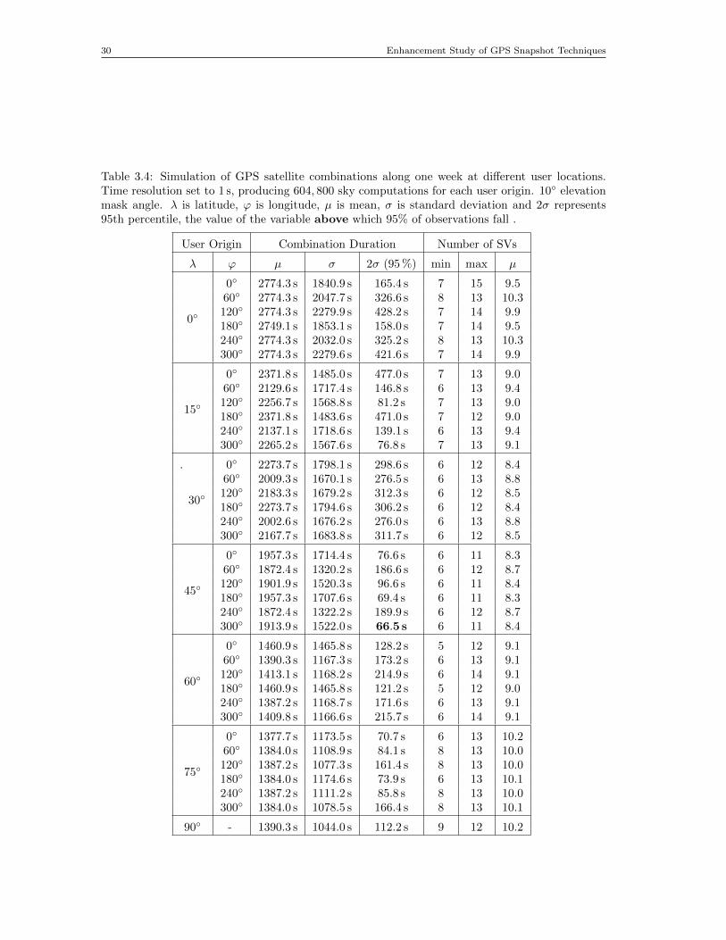
Eventually, a better solution came up through simulations of the visible satellites along a wholeweek. Results of these simulations for different user locations are presented in Table 3.4 providingpractical information on the duration of combinations.
At the Equator and low latitudes, we observe that there are between 7 and 15 satellites in view.The mean number of visible satellites around the globe is close to 9, which is another argument todiscard the first approximation.
In conclusion, coarse-time step was set to 1 minute in order to ensure getting at least 95% of thepossible combinations.
3.4 3.6 3.8 4 4.2 4.4
x 105
0
1
2
3
4
5
6
7
8
9
TW [s]
Num
ber
of c
oinc
iden
t SV
s
Figure 3.10: Number of coincident satellites along day. Results of coarse search for snapshot “2C”
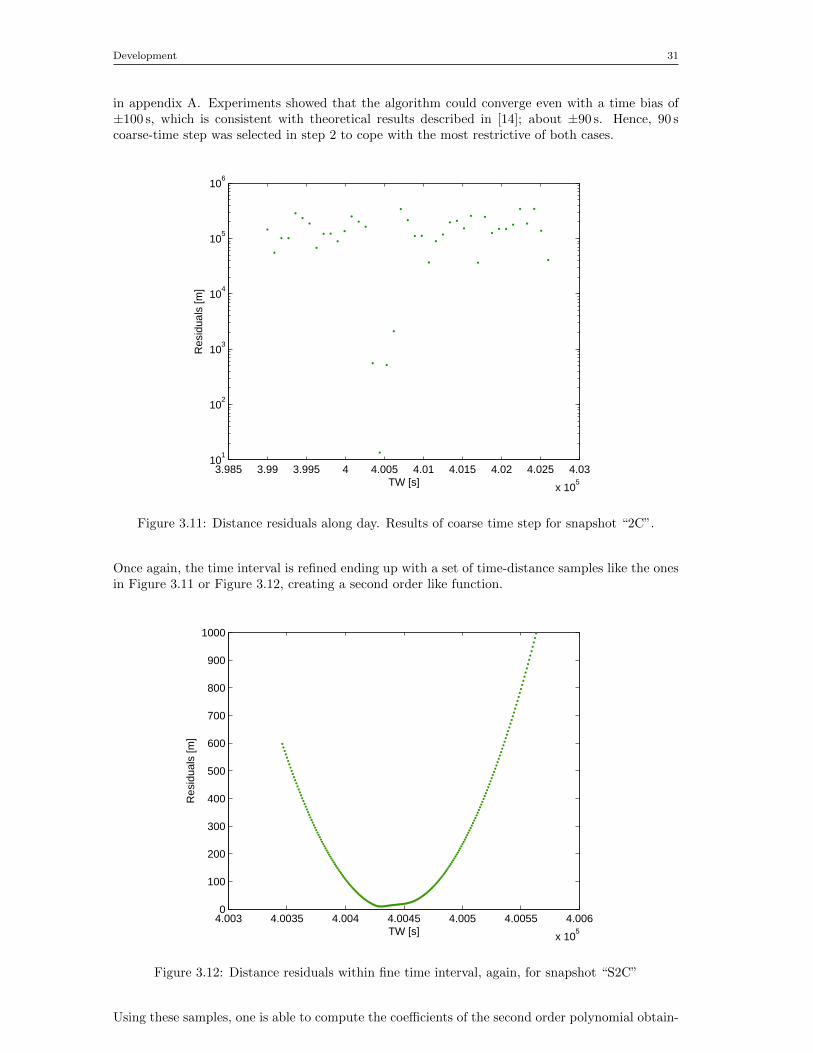
After the time interval in step 1 has been refined, a second search within it starts in step 2. Thistime we are taking advantage of the convergence properties of the coarse-time algorithm described
30 Enhancement Study of GPS Snapshot Techniques
Table 3.4: Simulation of GPS satellite combinations along one week at different user locations.Time resolution set to 1 s, producing 604, 800 sky computations for each user origin. 10◦ elevationmask angle. λ is latitude, ϕ is longitude, µ is mean, σ is standard deviation and 2σ represents95th percentile, the value of the variable above which 95% of observations fall .
User Origin Combination Duration Number of SVs
λ ϕ µ σ 2σ (95 %) min max µ
0◦
0◦ 2774.3 s 1840.9 s 165.4 s 7 15 9.560◦ 2774.3 s 2047.7 s 326.6 s 8 13 10.3120◦ 2774.3 s 2279.9 s 428.2 s 7 14 9.9180◦ 2749.1 s 1853.1 s 158.0 s 7 14 9.5240◦ 2774.3 s 2032.0 s 325.2 s 8 13 10.3300◦ 2774.3 s 2279.6 s 421.6 s 7 14 9.9
15◦
0◦ 2371.8 s 1485.0 s 477.0 s 7 13 9.060◦ 2129.6 s 1717.4 s 146.8 s 6 13 9.4120◦ 2256.7 s 1568.8 s 81.2 s 7 13 9.0180◦ 2371.8 s 1483.6 s 471.0 s 7 12 9.0240◦ 2137.1 s 1718.6 s 139.1 s 6 13 9.4300◦ 2265.2 s 1567.6 s 76.8 s 7 13 9.1
.
30◦
0◦ 2273.7 s 1798.1 s 298.6 s 6 12 8.460◦ 2009.3 s 1670.1 s 276.5 s 6 13 8.8120◦ 2183.3 s 1679.2 s 312.3 s 6 12 8.5180◦ 2273.7 s 1794.6 s 306.2 s 6 12 8.4240◦ 2002.6 s 1676.2 s 276.0 s 6 13 8.8300◦ 2167.7 s 1683.8 s 311.7 s 6 12 8.5
45◦
0◦ 1957.3 s 1714.4 s 76.6 s 6 11 8.360◦ 1872.4 s 1320.2 s 186.6 s 6 12 8.7120◦ 1901.9 s 1520.3 s 96.6 s 6 11 8.4180◦ 1957.3 s 1707.6 s 69.4 s 6 11 8.3240◦ 1872.4 s 1322.2 s 189.9 s 6 12 8.7300◦ 1913.9 s 1522.0 s 66.5 s 6 11 8.4
60◦
0◦ 1460.9 s 1465.8 s 128.2 s 5 12 9.160◦ 1390.3 s 1167.3 s 173.2 s 6 13 9.1120◦ 1413.1 s 1168.2 s 214.9 s 6 14 9.1180◦ 1460.9 s 1465.8 s 121.2 s 5 12 9.0240◦ 1387.2 s 1168.7 s 171.6 s 6 13 9.1300◦ 1409.8 s 1166.6 s 215.7 s 6 14 9.1
75◦
0◦ 1377.7 s 1173.5 s 70.7 s 6 13 10.260◦ 1384.0 s 1108.9 s 84.1 s 8 13 10.0120◦ 1387.2 s 1077.3 s 161.4 s 8 13 10.0180◦ 1384.0 s 1174.6 s 73.9 s 6 13 10.1240◦ 1387.2 s 1111.2 s 85.8 s 8 13 10.0300◦ 1384.0 s 1078.5 s 166.4 s 8 13 10.1
90◦ - 1390.3 s 1044.0 s 112.2 s 9 12 10.2
Development 31
in appendix A. Experiments showed that the algorithm could converge even with a time bias of±100 s, which is consistent with theoretical results described in [14]; about ±90 s. Hence, 90 scoarse-time step was selected in step 2 to cope with the most restrictive of both cases.
3.985 3.99 3.995 4 4.005 4.01 4.015 4.02 4.025 4.03
x 105
101
102
103
104
105
106
TW [s]
Res
idua
ls [m
]
Figure 3.11: Distance residuals along day. Results of coarse time step for snapshot “2C”.
Once again, the time interval is refined ending up with a set of time-distance samples like the onesin Figure 3.11 or Figure 3.12, creating a second order like function.
4.003 4.0035 4.004 4.0045 4.005 4.0055 4.006
x 105
0
100
200
300
400
500
600
700
800
900
1000
TW [s]
Res
idua
ls [m
]
Figure 3.12: Distance residuals within fine time interval, again, for snapshot “S2C”
Using these samples, one is able to compute the coefficients of the second order polynomial obtain-
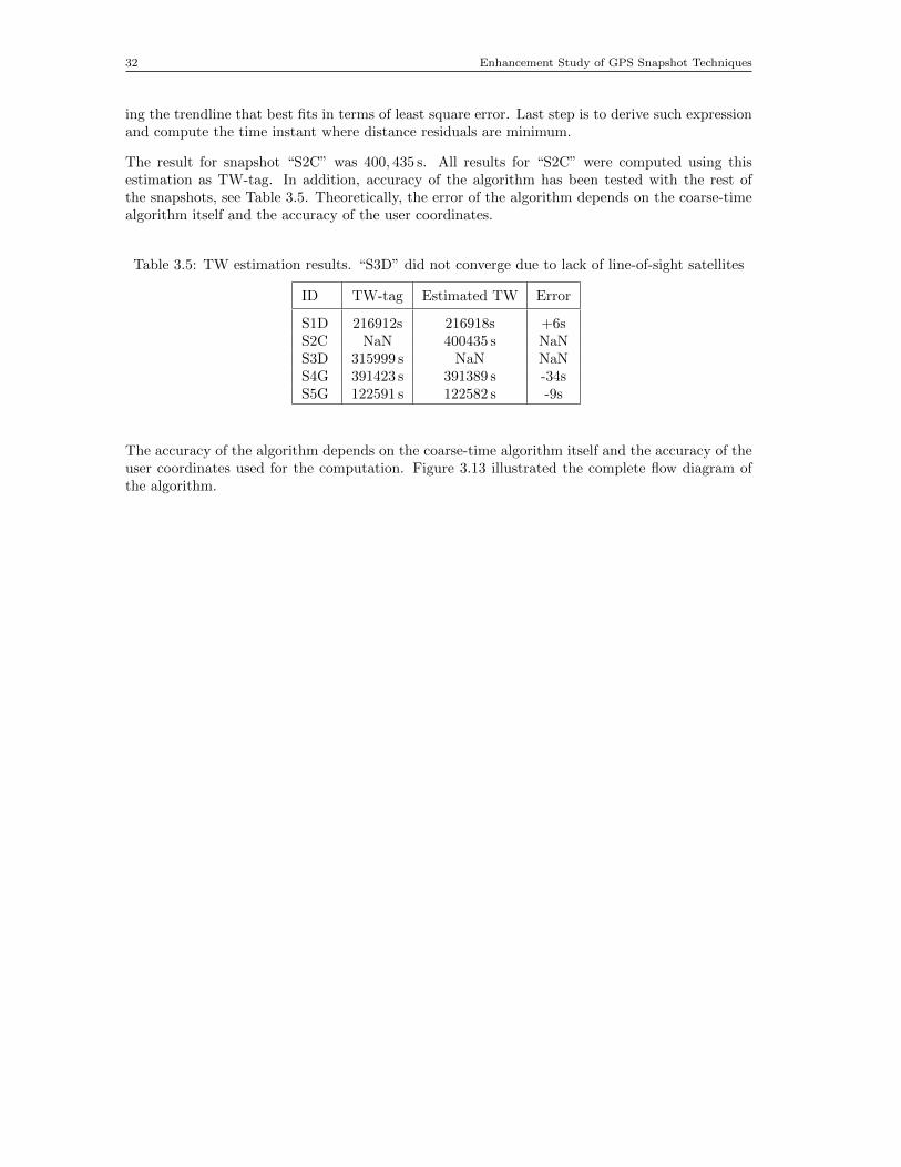
32 Enhancement Study of GPS Snapshot Techniques
ing the trendline that best fits in terms of least square error. Last step is to derive such expressionand compute the time instant where distance residuals are minimum.
The result for snapshot “S2C” was 400, 435 s. All results for “S2C” were computed using thisestimation as TW-tag. In addition, accuracy of the algorithm has been tested with the rest ofthe snapshots, see Table 3.5. Theoretically, the error of the algorithm depends on the coarse-timealgorithm itself and the accuracy of the user coordinates.
Table 3.5: TW estimation results. “S3D” did not converge due to lack of line-of-sight satellites
ID TW-tag Estimated TW Error
S1D 216912s 216918s +6sS2C NaN 400435 s NaNS3D 315999 s NaN NaNS4G 391423 s 391389 s -34sS5G 122591 s 122582 s -9s
The accuracy of the algorithm depends on the coarse-time algorithm itself and the accuracy of theuser coordinates used for the computation. Figure 3.13 illustrated the complete flow diagram ofthe algorithm.
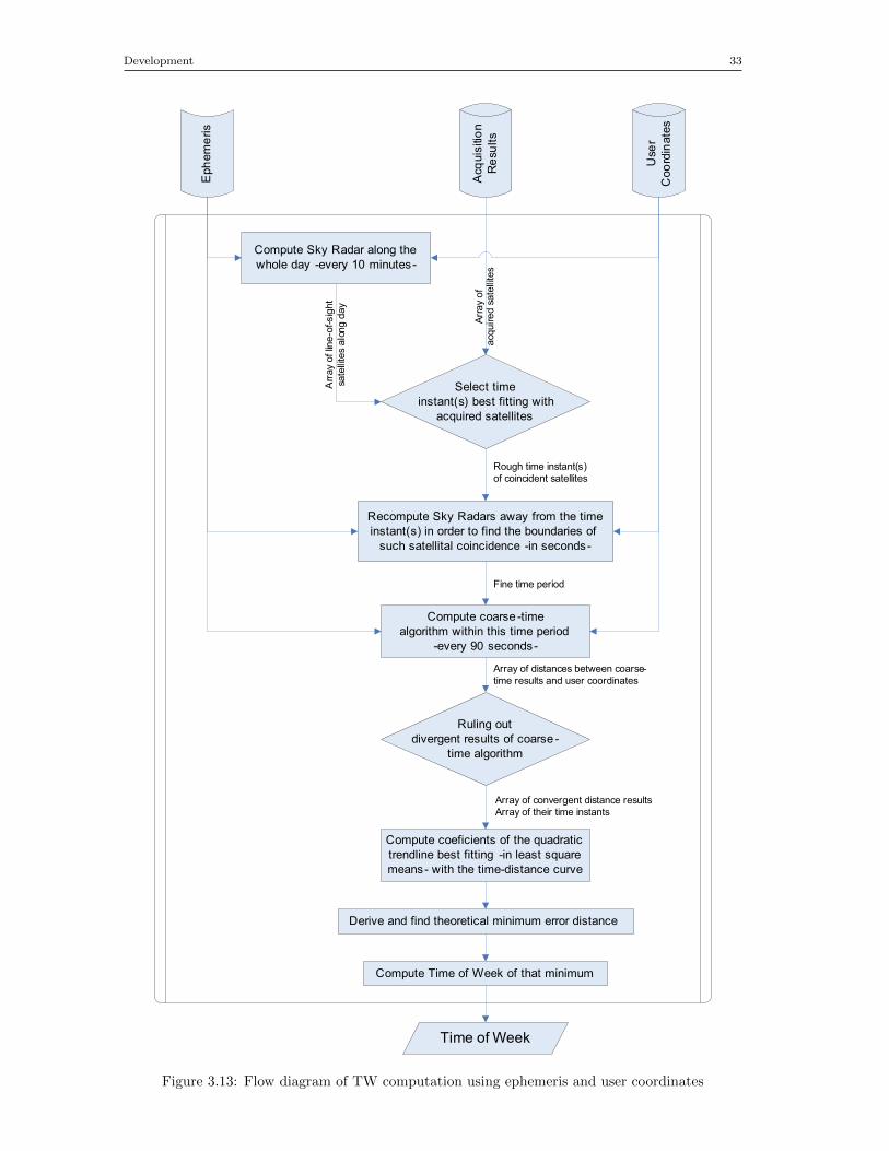
Development 33
Eph
em
eris
Acq
uis
itio
n
Re
sults
Use
r
Coo
rdin
ate
s
Compute Sky Radar along the
whole day -every 10 minutes-
Arr
ay o
f acq
uired s
ate
llite
s
Arr
ay
of lin
e-o
f-sig
ht
sate
llite
s alo
ng d
ay
Recompute Sky Radars away from the time
instant(s) in order to find the boundaries of
such satellital coincidence -in seconds-
Compute coarse -time
algorithm within this time period
-every 90 seconds-
Rough time instant(s)
of coincident satellites
Fine time period
Select time
instant(s) best fitting with
acquired satellites
Ruling out
divergent results of coarse -
time algorithm
Array of distances between coarse-
time results and user coordinates
Array of convergent distance results
Array of their time instants
Compute coeficients of the quadratic
trendline best fitting -in least square
means- with the time-distance curve
Derive and find theoretical minimum error distance
Compute Time of Week of that minimum
Time of Week
Figure 3.13: Flow diagram of TW computation using ephemeris and user coordinates
34 Enhancement Study of GPS Snapshot Techniques
3.2.2 Ephemerides
Ephemerides contain information about Keplerian elements plus corrections for the Earth’s grav-itational field and other forces [9], providing time dependent, accurate satellite orbit values. In aclassic GPS hardware receiver, obtaining ephemerides is only possible after tracking. Due to thefact that snapshot techniques do not perform tracking, ephemeris have to be supplied by othermeans.
In the code presented with [5], ephemeris were manually assisted as well as time. In practice, thereare several file formats designed to broadcast information about GPS satellites orbits. Perhaps,the most popular ones are:
• YUMA almanac: Contains the six basic Keplerian elements describing orbits in the long-term. It is not accurate.
• RINEX navigation files: Collection of ephemeris broadcasted by the constellation within agiven period of time. For 24 h RINEX navigation files, for instance, ephemerides for thedifferent satellites are updated, at least, every 4 h. Inside this 2 to 4 h period, ephemeridesprovide best fit with the real satellite trajectory thanks to some additional correction parame-ters applied on top of the almanac. Ephemerides provide satellite positioning with sub-meteraccuracy.
From the beginning, 24 h broadcast RINEX navigation files where selected for being the most accu-rate and widely used standard files, although suffering from very low update cadence (daily). Theyare available from public databases such as the Interntional GNSS Service (IGS) or other publicentities offering GPS data services. Typically, the contents of these databases are automaticallysorted by date and all files are named following a known pattern. Taking advantage of this fact,and assuming that the snapshot date is known, it was relatively easy to implement an automaticassistance of ephemeris, releasing the user of this task.
In our particular application, all navigation files are retrieved from CDDIS (Crustal DynamicsData Information System) database. There files are sorted using a tree like structure of foldersaccording to: ftp://cddis.gsfc.nasa.gov/pub/gps/data/daily/YYYY/brdc/brdcDDD0.YYn.Z,where “YYYY” is 4 digit number of year, “DDD” is 3 digit day number (0 padding in the lefthand side might be required) “YY” is 2 last digits of the year and “n” indicates navigation file.One limitation of this solution might be that the user has to wait until the files are published (after24 h in the worst case) before being able to compute positioning of the snapshot. Nevertheless, itis possible to find hourly data files also using RINEX format and it has been considered a goodacademical exercise to use them and get used to their structure.
Eventually, only a priori position is remaining to be manually introduced as an input to thealgorithm.
3.2.3 Computing First Fix from Doppler Measurements
This algorithm is intended to solve for a position first fix using instant Doppler measurements. In[5] the user should have introduced an initial position manually in order to solve for its positionwith the coarse time navigation algorithm. As stated in 1 one of our purposes is to make theapplication as transparent to the user as possible. This is why we have chosen to apply Dopplermeasurements for computing an initial position.
Firstly we had to investigate if the Doppler positioning is able to provide us with a position withinthe accuracy range that is needed by the other algorithms. In [5] it was also shown that thisinitial position can vary in a range of ±150 km without affecting the capacity of the coarse timealgorithm to converge and provide an position accurate within 20 − 50 m. Reference [14] statesthat the purpose of the Doppler navigation is to provide a first fix better than 150 km. Thereforewe decided that this method is suitable for our application.
Development 35
We pursued to implement the algorithm presented in [14] by first starting from the linear navigationequation which relates pseudo-ranges to the state update, already presented in (3.19). In order tohave Doppler measurements we must differentiate it with respect to time. Therefore we get (boldcharacters represent vectors):
∂δz
∂t=∂(Hδx)
∂t+ ε′ (3.28)
∂(z− z)
∂t=∂(Hδx)
∂t+ ε′ (3.29)
∂z
∂t− ∂z
∂t= H
∂(δx)
∂t+∂(H)
∂tδx + ε′ (3.30)
The left side is identified as the vector of a priori Doppler measurement residuals δy = y− y. Wecontinue with the next notations:
y = ∂z/∂t is the vector of measured Dopplery = ∂z/∂t is the vector of predicted Doppler based on satellite-user motion
In order to be able to follow the equations more easily we consider the two terms in the right sideseparately. Therefore the first term will be:
H∂(δx)
∂t= H
∂
∂t
δxδyδzδb
= H
δx′
δy′
δz′
δb′
=
−e1 1
......
−ei 1
δx′
δy′
δz′
δb′
(3.31)
where:δx′ , δy′ and δz′ represent the updates to the a priori receiver velocity states.δb′ is the update to the a priori frequency state.
The second right hand term of equation 3.30 will provide us with the necessary relationship betweenposition and Doppler measurements:
∂H
∂tδx =
∂
∂t
−e1 1
......
−ei 1
δxδyδzδb
=
−∂e1
∂t 0...
...−∂ei∂t 0
δxδyδzδb
=
−∂e1
∂t...−∂ei∂t
δxδyδz
(3.32)
ei = [exi; ey
i; ezi] is the unit vector in the direction from the receiver to satellite i. Therefore we
must find an explicit expression for the vector −∂ei/∂t:
∂ei
∂t=
∂
∂t
(xi − x0
|xi − x0|
)(3.33)
where:xi is the position of satellite ix0 is the apriori position of the receiver
36 Enhancement Study of GPS Snapshot Techniques
Solving (3.33) becomes:
∂ei
∂t=
(∂xi − x0
∂t.|xi − x0| −
(xi − x0
).∂|xi − x0|
∂t
)1
|xi − x0|2
=
(∂(xi)
∂t.|xi − x0| −
(xi − x0
).(ei • vi
)) 1
|xi − x0|2
=
(∂(xi)
∂t.|xi − x0| − |xi − x0|.ei.
(ei • vi
)) 1
|xi − x0|2
=
(∂(xi)
∂t− ei.
(ei • vi
)) 1
|xi − x0|
This means that the derivation in time of the unit vector equals to the difference between therelative satellite velocity and the satellite velocity component in direction of line-of-sigh, dividedby the range.
Therefore we have all the components we need in order to solve (3.30) which becomes:
δy =
−e1 1
......
−ei 1
δx′
δy′
δz′
δb′
+
−∂e1
∂t...−∂ei∂t
δxδyδz
+ ε′ (3.34)
Eventually, we obtain a linear equation with seven unknowns and, in order to solve through leastsquares, we desire to have all the unknowns grouped in the same term:
δy =
−e1 1 −∂e1
∂t...
......
−ei 1 −∂ei∂t
δx′
δy′
δz′
δb′
δxδyδz
+ ε′ (3.35)
Theoretically, if the receiver is stationary, δx′ , δy′ and δz′ equal to zero, then the system reducesto four unknowns:
δy =
−∂e1
∂t 1...
...−∂ei∂t 1
δxδyδzδb′
+ ε′ (3.36)
3.3 Summary
This chapter was devoted to describing the theory and implementation methods for the two maindirections of the present project:
• Improving accuracy
• Providing auto-assistance
Concerning accuracy improvement this chapter contained a description of the tracking algorithmswe have implemented, it showed the method of solving for ionospheric delay,by using IONEX, and

Development 37
for tropospheric delay, and it described how to get URA indeces and how they are used as weightsin a weighted least squares solution.
The auto-assistance section covered the description of how we successfully provided assisted timeto the positioning algorithms and described a new method to estimate TOW. Furthermore thissection described how ephemerides were automatically provided. The last subject we approachedwas a description of the Doppler navigation algorithm implementation.

38 Enhancement Study of GPS Snapshot Techniques
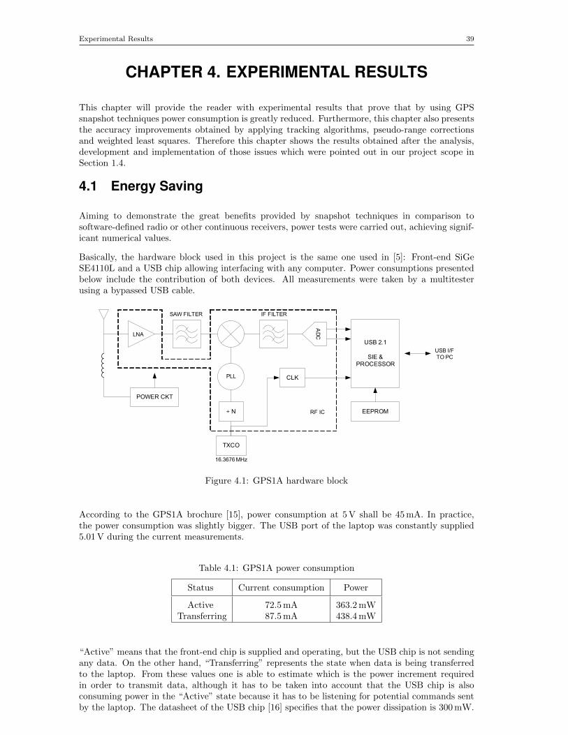
Experimental Results 39
CHAPTER 4. EXPERIMENTAL RESULTS
This chapter will provide the reader with experimental results that prove that by using GPSsnapshot techniques power consumption is greatly reduced. Furthermore, this chapter also presentsthe accuracy improvements obtained by applying tracking algorithms, pseudo-range correctionsand weighted least squares. Therefore this chapter shows the results obtained after the analysis,development and implementation of those issues which were pointed out in our project scope inSection 1.4.
4.1 Energy Saving
Aiming to demonstrate the great benefits provided by snapshot techniques in comparison tosoftware-defined radio or other continuous receivers, power tests were carried out, achieving signif-icant numerical values.
Basically, the hardware block used in this project is the same one used in [5]: Front-end SiGeSE4110L and a USB chip allowing interfacing with any computer. Power consumptions presentedbelow include the contribution of both devices. All measurements were taken by a multitesterusing a bypassed USB cable.
PLL
TXCO
EEPROM÷ N
CLK
USB 2.1
SIE & PROCESSOR
POWER CKT
LNA
SAW FILTER
AD
C
IF FILTER
16.3676 MHz
RF IC
USB I/F
TO PC
Figure 4.1: GPS1A hardware block
According to the GPS1A brochure [15], power consumption at 5 V shall be 45 mA. In practice,the power consumption was slightly bigger. The USB port of the laptop was constantly supplied5.01 V during the current measurements.
Table 4.1: GPS1A power consumption
Status Current consumption Power
Active 72.5 mA 363.2 mWTransferring 87.5 mA 438.4 mW
“Active” means that the front-end chip is supplied and operating, but the USB chip is not sendingany data. On the other hand, “Transferring” represents the state when data is being transferredto the laptop. From these values one is able to estimate which is the power increment requiredin order to transmit data, although it has to be taken into account that the USB chip is alsoconsuming power in the “Active” state because it has to be listening for potential commands sentby the laptop. The datasheet of the USB chip [16] specifies that the power dissipation is 300 mW.
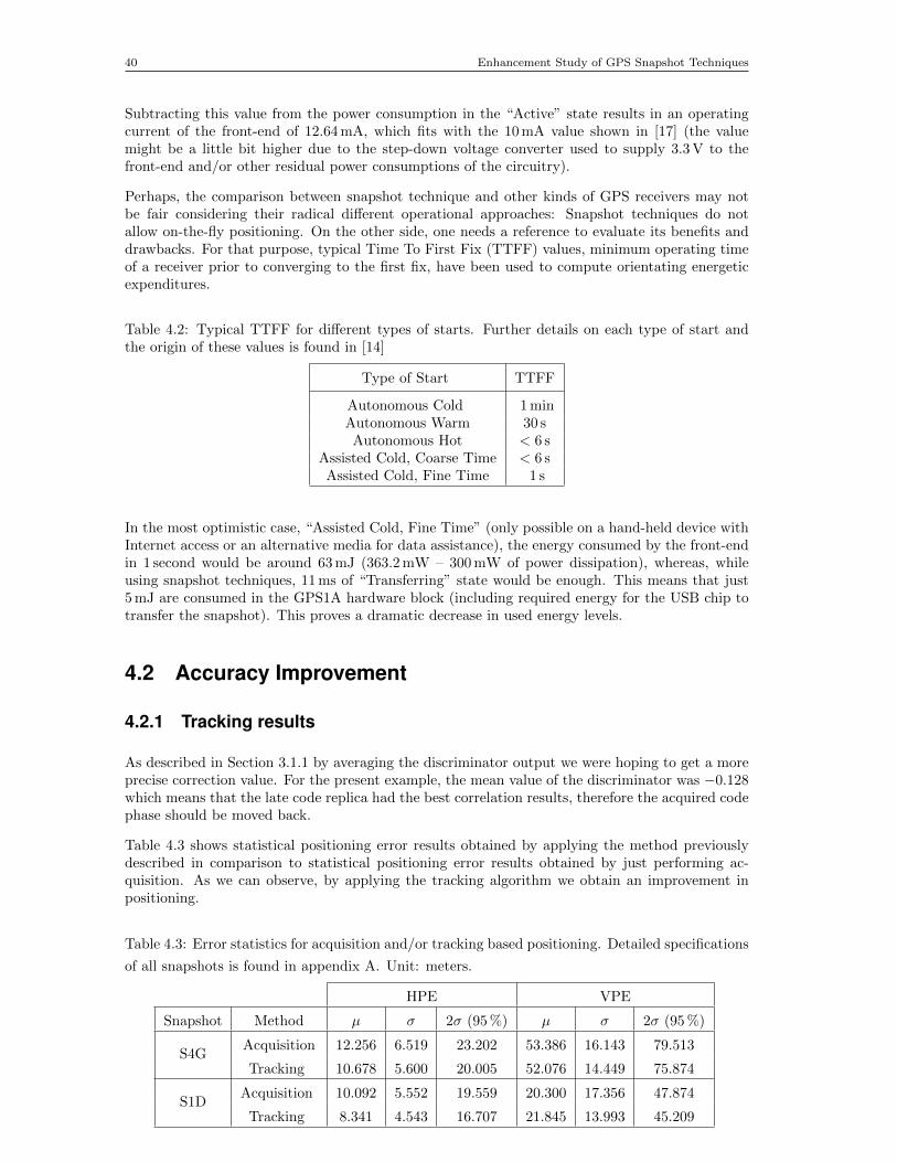
40 Enhancement Study of GPS Snapshot Techniques
Subtracting this value from the power consumption in the “Active” state results in an operatingcurrent of the front-end of 12.64 mA, which fits with the 10 mA value shown in [17] (the valuemight be a little bit higher due to the step-down voltage converter used to supply 3.3 V to thefront-end and/or other residual power consumptions of the circuitry).
Perhaps, the comparison between snapshot technique and other kinds of GPS receivers may notbe fair considering their radical different operational approaches: Snapshot techniques do notallow on-the-fly positioning. On the other side, one needs a reference to evaluate its benefits anddrawbacks. For that purpose, typical Time To First Fix (TTFF) values, minimum operating timeof a receiver prior to converging to the first fix, have been used to compute orientating energeticexpenditures.
Table 4.2: Typical TTFF for different types of starts. Further details on each type of start andthe origin of these values is found in [14]
Type of Start TTFF
Autonomous Cold 1 minAutonomous Warm 30 sAutonomous Hot < 6 s
Assisted Cold, Coarse Time < 6 sAssisted Cold, Fine Time 1 s
In the most optimistic case, “Assisted Cold, Fine Time” (only possible on a hand-held device withInternet access or an alternative media for data assistance), the energy consumed by the front-endin 1 second would be around 63 mJ (363.2 mW – 300 mW of power dissipation), whereas, whileusing snapshot techniques, 11 ms of “Transferring” state would be enough. This means that just5 mJ are consumed in the GPS1A hardware block (including required energy for the USB chip totransfer the snapshot). This proves a dramatic decrease in used energy levels.
4.2 Accuracy Improvement
4.2.1 Tracking results
As described in Section 3.1.1 by averaging the discriminator output we were hoping to get a moreprecise correction value. For the present example, the mean value of the discriminator was −0.128which means that the late code replica had the best correlation results, therefore the acquired codephase should be moved back.
Table 4.3 shows statistical positioning error results obtained by applying the method previouslydescribed in comparison to statistical positioning error results obtained by just performing ac-quisition. As we can observe, by applying the tracking algorithm we obtain an improvement inpositioning.
Table 4.3: Error statistics for acquisition and/or tracking based positioning. Detailed specifications
of all snapshots is found in appendix A. Unit: meters.
HPE VPE
Snapshot Method µ σ 2σ (95 %) µ σ 2σ (95 %)
S4GAcquisition 12.256 6.519 23.202 53.386 16.143 79.513
Tracking 10.678 5.600 20.005 52.076 14.449 75.874
S1DAcquisition 10.092 5.552 19.559 20.300 17.356 47.874
Tracking 8.341 4.543 16.707 21.845 13.993 45.209
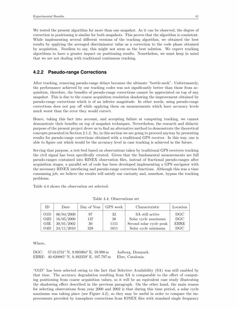
Experimental Results 41
We tested the present algorithm for more than one snapshot. As it can be observed, the degree ofcorrection in positioning is similar for both snapshots. This proves that the algorithm is consistent.While implementing several different versions of the tracking algorithm, we obtained the bestresults by applying the averaged discriminator value as a correction to the code phase obtainedby acquisition. Needless to say, this might not seem as the best solution. We expect trackingalgorithms to have a greater impact on positioning results. Nonetheless, we must keep in mindthat we are not dealing with traditional continuous tracking.
4.2.2 Pseudo-range Corrections
After tracking, removing pseudo-range delays becomes the ultimate “bottle-neck”. Unfortunately,the performance achieved by our tracking codes was not significantly better than those from ac-quisition, therefore, the benefits of pseudo-range corrections cannot be appreciated on top of anysnapshot. This is due to the coarse acquisition resolution shadowing the improvement obtained bypseudo-range corrections which is of an inferior magnitude. In other words, using pseudo-rangecorrections does not pay off while applying them on measurements which have accuracy levelsmuch worst than the error they would correct.
Hence, taking this fact into account, and accepting failure at computing tracking, we cannotdemonstrate their benefits on top of snapshot techniques. Nevertheless, the research and didacticpurpose of the present project drove us to find an alternative method to demonstrate the theoreticalconcepts presented in Section 2.1.2. So, in this section we are going to proceed anyway by presentingresults for pseudo-range corrections obtained with a traditional GPS receiver. In this way, one isable to figure out which would be the accuracy level in case tracking is achieved in the future.
Serving that purpose, a test-bed based on observations taken by traditional GPS receivers trackingthe civil signal has been specifically created. Given that the fundamental measurements are fullpseudo-ranges contained into RINEX observation files, instead of fractional pseudo-ranges afteracquisition stages, a parallel set of code has been developed implementing a GPS navigator withthe necessary RINEX interfacing and pseudo-range correction functions. Although this was a timeconsuming job, we believe the results will satisfy our curiosity and, somehow, bypass the trackingproblems.
Table 4.4 shows the observation set selected:
Table 4.4: Observations set
ID Date Day of Year GPS week Characteristic Location
O1D 06/04/2000 97 32 SA still active DGCO2D 16/05/2000 137 38 Solar cycle maximum DGCO3E 30/01/2002 30 1151 Second solar cycle peak EBREO4D 24/11/2010 328 1611 Solar cycle minimum DGC
Where,
DGC: 57.014731◦N, 9.985904◦ E, 59.998 m Aalborg, Denmark.EBRE: 40.820885◦N, 0.492359◦ E, 107.797 m Ebre, Catalonia.
“O1D” has been selected owing to the fact that Selective Availability (SA) was still enabled bythat time. The accuracy degradation resulting from SA is comparable to the effect of comput-ing positioning from coarse acquisition values, so it will be an equivalent case study illustratingthe shadowing effect described in the previous paragraph. On the other hand, the main reasonfor selecting observations from year 2000 and 2002 is that during this time period, a solar cyclemaximum was taking place (see Figure 4.2), so they may be useful in order to compare the im-provements provided by ionosphere corrections from IONEX files with standard single frequency
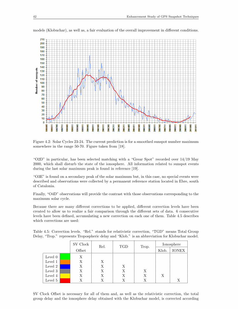
42 Enhancement Study of GPS Snapshot Techniques
models (Klobuchar), as well as, a fair evaluation of the overall improvement in different conditions.
Figure 4.2: Solar Cycles 23-24. The current prediction is for a smoothed sunspot number maximumsomewhere in the range 50-70. Figure taken from [18].
“O2D” in particular, has been selected matching with a “Grear Spot” recorded over 14/19 May2000, which shall disturb the state of the ionosphere. All information related to sunspot eventsduring the last solar maximum peak is found in reference [19].
“O3E” is found on a secondary peak of the solar maximum but, in this case, no special events weredescribed and observations were collected by a permanent reference station located in Ebre, southof Catalonia.
Finally, “O4D” observations will provide the contrast with those observations corresponding to themaximum solar cycle.
Because there are many different corrections to be applied, different correction levels have beencreated to allow us to realize a fair comparison through the different sets of data. 6 consecutivelevels have been defined, accumulating a new correction on each one of them. Table 4.5 describeswhich corrections are used:
Table 4.5: Correction levels. “Rel.” stands for relativistic correction, “TGD” means Total GroupDelay, “Trop.” represents Tropospheric delay and “Klob.” is an abbreviation for Klobuchar model.
SV ClockRel. TGD Trop.
Ionosphere
Offset Klob. IONEX
Level 0 XLevel 1 X XLevel 2 X X XLevel 3 X X X XLevel 4 X X X X XLevel 5 X X X X X
SV Clock Offset is necessary for all of them and, as well as the relativistic correction, the totalgroup delay and the ionosphere delay obtained with the Klobuchar model, is corrected according
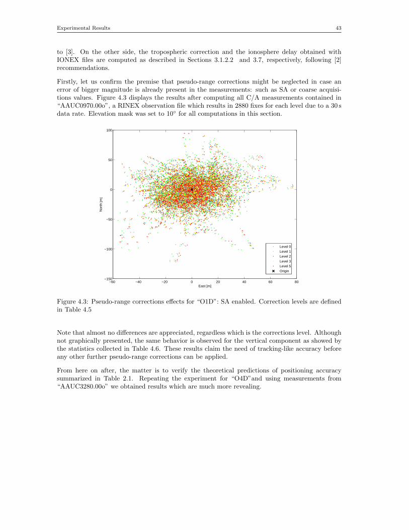
Experimental Results 43
to [3]. On the other side, the tropospheric correction and the ionosphere delay obtained withIONEX files are computed as described in Sections 3.1.2.2 and 3.7, respectively, following [2]recommendations.
Firstly, let us confirm the premise that pseudo-range corrections might be neglected in case anerror of bigger magnitude is already present in the measurements: such as SA or coarse acquisi-tions values. Figure 4.3 displays the results after computing all C/A measurements contained in“AAUC0970.00o”, a RINEX observation file which results in 2880 fixes for each level due to a 30 sdata rate. Elevation mask was set to 10◦ for all computations in this section.
−60 −40 −20 0 20 40 60 80−150
−100
−50
0
50
100
East [m]
Nor
th [m
]
Level 0Level 1Level 2Level 3Level 5Origin
Figure 4.3: Pseudo-range corrections effects for “O1D”: SA enabled. Correction levels are definedin Table 4.5
Note that almost no differences are appreciated, regardless which is the corrections level. Althoughnot graphically presented, the same behavior is observed for the vertical component as showed bythe statistics collected in Table 4.6. These results claim the need of tracking-like accuracy beforeany other further pseudo-range corrections can be applied.
From here on after, the matter is to verify the theoretical predictions of positioning accuracysummarized in Table 2.1. Repeating the experiment for “O4D”and using measurements from“AAUC3280.00o” we obtained results which are much more revealing.
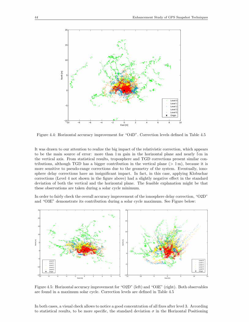
44 Enhancement Study of GPS Snapshot Techniques
−10 −8 −6 −4 −2 0 2 4 6 8 10−10
−5
0
5
10
15
20
East [m]
Nor
th [m
]
Level 0Level 1Level 2Level 3Level 5Origin
Figure 4.4: Horizontal accuracy improvement for “O4D”. Correction levels defined in Table 4.5
It was drawn to our attention to realize the big impact of the relativistic correction, which appearsto be the main source of error: more than 1 m gain in the horizontal plane and nearly 5 m inthe vertical axis. From statistical results, troposphere and TGD corrections present similar con-tributions, although TGD has a bigger contribution in the vertical plane (> 1 m), because it ismore sensitive to pseudo-range corrections due to the geometry of the system. Eventually, iono-sphere delay corrections have an insignificant impact. In fact, in this case, applying Klobucharcorrections (Level 4 not shown in the figure above) had a slightly negative effect in the standarddeviation of both the vertical and the horizontal plane. The feasible explanation might be thatthese observations are taken during a solar cycle minimum.
In order to fairly check the overall accuracy improvement of the ionosphere delay correction, “O2D”and “O3E” demonstrate its contribution during a solar cycle maximum. See Figure below:
−10 −8 −6 −4 −2 0 2 4 6 8−15
−10
−5
0
5
10
15
20
25
East [m]
Nor
th [m
]
Level 0Level 1Level 2Level 3Level 5Origin
−15 −10 −5 0 5 10 15−10
−5
0
5
10
15
20
East [m]
Nor
th [m
]
Level 0Level 1Level 2Level 3Level 5Origin
Figure 4.5: Horizontal accuracy improvement for “O2D” (left) and “O3E” (right). Both observablesare found in a maximum solar cycle. Correction levels are defined in Table 4.5
In both cases, a visual check allows to notice a good concentration of all fixes after level 3. Accordingto statistical results, to be more specific, the standard deviation σ in the Horizontal Positioning
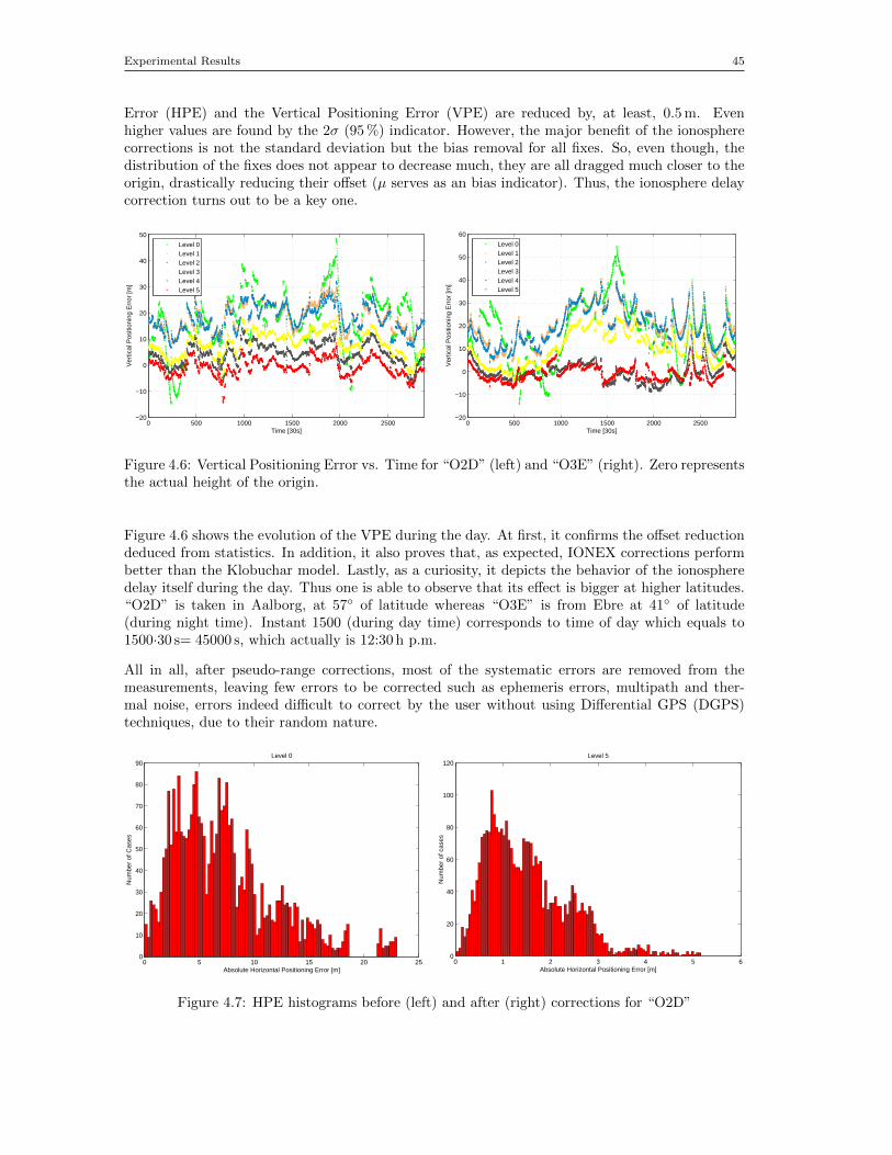
Experimental Results 45
Error (HPE) and the Vertical Positioning Error (VPE) are reduced by, at least, 0.5 m. Evenhigher values are found by the 2σ (95 %) indicator. However, the major benefit of the ionospherecorrections is not the standard deviation but the bias removal for all fixes. So, even though, thedistribution of the fixes does not appear to decrease much, they are all dragged much closer to theorigin, drastically reducing their offset (µ serves as an bias indicator). Thus, the ionosphere delaycorrection turns out to be a key one.
0 500 1000 1500 2000 2500−20
−10
0
10
20
30
40
50
Time [30s]
Ver
tical
Pos
ition
ing
Err
or [m
]
0 500 1000 1500 2000 2500−20
−10
0
10
20
30
40
50
60
Time [30s]
Ver
tical
Pos
ition
ing
Err
or [m
]
Level 0Level 1Level 2Level 3Level 4Level 5
Level 0Level 1Level 2Level 3Level 4Level 5
Figure 4.6: Vertical Positioning Error vs. Time for “O2D” (left) and “O3E” (right). Zero representsthe actual height of the origin.
Figure 4.6 shows the evolution of the VPE during the day. At first, it confirms the offset reductiondeduced from statistics. In addition, it also proves that, as expected, IONEX corrections performbetter than the Klobuchar model. Lastly, as a curiosity, it depicts the behavior of the ionospheredelay itself during the day. Thus one is able to observe that its effect is bigger at higher latitudes.“O2D” is taken in Aalborg, at 57◦ of latitude whereas “O3E” is from Ebre at 41◦ of latitude(during night time). Instant 1500 (during day time) corresponds to time of day which equals to1500·30 s= 45000 s, which actually is 12:30 h p.m.
All in all, after pseudo-range corrections, most of the systematic errors are removed from themeasurements, leaving few errors to be corrected such as ephemeris errors, multipath and ther-mal noise, errors indeed difficult to correct by the user without using Differential GPS (DGPS)techniques, due to their random nature.
0 5 10 15 20 250
10
20
30
40
50
60
70
80
90
Absolute Horizontal Positioning Error [m]
Num
ber
of C
ases
Level 0
0 1 2 3 4 5 60
20
40
60
80
100
120Level 5
Absolute Horizontal Positioning Error [m]
Num
ber
of c
ases
Figure 4.7: HPE histograms before (left) and after (right) corrections for “O2D”
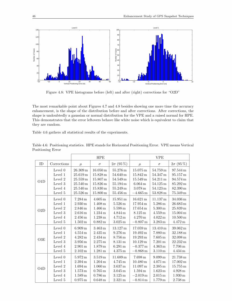
46 Enhancement Study of GPS Snapshot Techniques
−20 −10 0 10 20 30 40 500
20
40
60
80
100
120
140
Vertical Positioning Error [m]
Num
ber
of C
ases
Level 0
−15 −10 −5 0 5 100
10
20
30
40
50
60
70
80
90
100Level 5
Vertical Positioning Error [m]
Num
ber
of C
ases
Figure 4.8: VPE histograms before (left) and after (right) corrections for “O2D”
The most remarkable point about Figures 4.7 and 4.8 besides showing one more time the accuracyenhancement, is the shape of the distribution before and after corrections. After corrections, theshape is undoubtedly a gaussian or normal distribution for the VPE and a raised normal for HPE.This demonstrates that the error leftovers behave like white noise which is equivalent to claim thatthey are random.
Table 4.6 gathers all statistical results of the experiments.
Table 4.6: Positioning statistics. HPE stands for Horizontal Positioning Error. VPE means VerticalPositioning Error
HPE VPE
ID Corrections µ σ 2σ (95 %) µ σ 2σ (95 %)
O1D
Level 0 26.309 m 16.050 m 55.276 m 15.075 m 54.759 m 97.544 mLevel 1 25.619 m 15.828 m 54.640 m 15.842 m 54.347 m 95.157 mLevel 2 25.559 m 15.807 m 54.549 m 15.549 m 54.211 m 94.574 mLevel 3 25.540 m 15.826 m 55.194 m 6.064 m 54.125 m 85.292 mLevel 4 25.540 m 15.830 m 55.249 m 3.078 m 54.123 m 82.390 mLevel 5 25.526 m 15.800 m 55.456 m −4.665 m 53.828 m 75.349 m
O2D
Level 0 7.284 m 4.605 m 15.951 m 16.621 m 11.137 m 34.036 mLevel 1 2.930 m 1.408 m 5.526 m 17.954 m 5.286 m 26.683 mLevel 2 2.846 m 1.466 m 5.598 m 17.654 m 5.300 m 25.839 mLevel 3 2.616 m 1.234 m 4.844 m 8.125 m 4.559 m 15.004 mLevel 4 2.456 m 1.238 m 4.712 m 4.270 m 4.022 m 10.500 mLevel 5 1.502 m 0.882 m 3.025 m −0.807 m 3.283 m 4.472 m
O3E
Level 0 6.909 m 3.463 m 13.127 m 17.059 m 13.410 m 39.062 mLevel 1 4.554 m 2.435 m 9.276 m 19.492 m 7.880 m 32.188 mLevel 2 4.282 m 2.434 m 8.756 m 19.293 m 7.605 m 32.098 mLevel 3 3.956 m 2.275 m 8.131 m 10.129 m 7.201 m 22.232 mLevel 4 2.901 m 1.879 m 6.291 m −0.377 m 4.363 m 7.706 mLevel 5 2.102 m 1.281 m 4.375 m −0.868 m 3.110 m 4.434 m
O4D
Level 0 5.972 m 3.519 m 11.689 m 7.698 m 9.099 m 21.738 mLevel 1 2.394 m 1.204 m 4.745 m 10.480 m 4.071 m 17.002 mLevel 2 1.694 m 1.060 m 3.637 m 11.097 m 2.385 m 15.755 mLevel 3 1.573 m 0.765 m 3.045 m 1.594 m 1.623 m 4.928 mLevel 4 1.589 m 0.786 m 3.125 m −2.019 m 2.015 m 1.930 mLevel 5 0.975 m 0.648 m 2.321 m −0.814 m 1.779 m 2.738 m
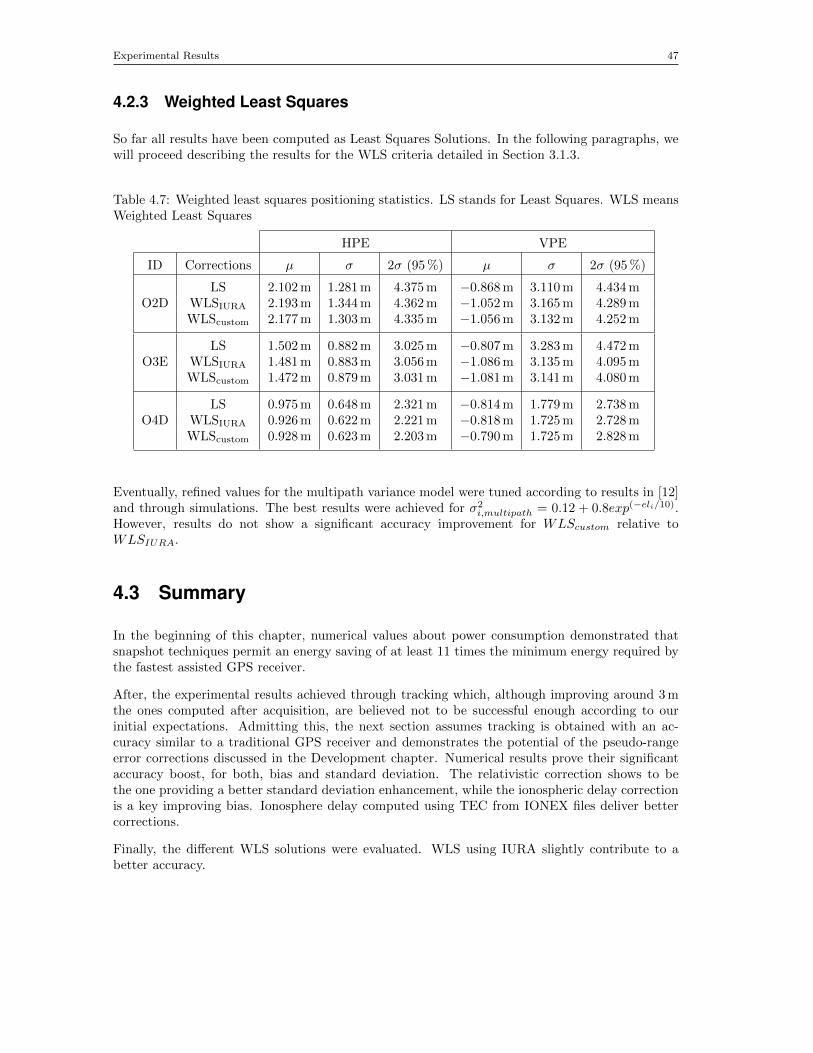
Experimental Results 47
4.2.3 Weighted Least Squares
So far all results have been computed as Least Squares Solutions. In the following paragraphs, wewill proceed describing the results for the WLS criteria detailed in Section 3.1.3.
Table 4.7: Weighted least squares positioning statistics. LS stands for Least Squares. WLS meansWeighted Least Squares
HPE VPE
ID Corrections µ σ 2σ (95 %) µ σ 2σ (95 %)
O2DLS 2.102 m 1.281 m 4.375 m −0.868 m 3.110 m 4.434 m
WLSIURA 2.193 m 1.344 m 4.362 m −1.052 m 3.165 m 4.289 mWLScustom 2.177 m 1.303 m 4.335 m −1.056 m 3.132 m 4.252 m
O3ELS 1.502 m 0.882 m 3.025 m −0.807 m 3.283 m 4.472 m
WLSIURA 1.481 m 0.883 m 3.056 m −1.086 m 3.135 m 4.095 mWLScustom 1.472 m 0.879 m 3.031 m −1.081 m 3.141 m 4.080 m
O4DLS 0.975 m 0.648 m 2.321 m −0.814 m 1.779 m 2.738 m
WLSIURA 0.926 m 0.622 m 2.221 m −0.818 m 1.725 m 2.728 mWLScustom 0.928 m 0.623 m 2.203 m −0.790 m 1.725 m 2.828 m
Eventually, refined values for the multipath variance model were tuned according to results in [12]and through simulations. The best results were achieved for σ2
i,multipath = 0.12 + 0.8exp(−eli/10).However, results do not show a significant accuracy improvement for WLScustom relative toWLSIURA.
4.3 Summary
In the beginning of this chapter, numerical values about power consumption demonstrated thatsnapshot techniques permit an energy saving of at least 11 times the minimum energy required bythe fastest assisted GPS receiver.
After, the experimental results achieved through tracking which, although improving around 3 mthe ones computed after acquisition, are believed not to be successful enough according to ourinitial expectations. Admitting this, the next section assumes tracking is obtained with an ac-curacy similar to a traditional GPS receiver and demonstrates the potential of the pseudo-rangeerror corrections discussed in the Development chapter. Numerical results prove their significantaccuracy boost, for both, bias and standard deviation. The relativistic correction shows to bethe one providing a better standard deviation enhancement, while the ionospheric delay correctionis a key improving bias. Ionosphere delay computed using TEC from IONEX files deliver bettercorrections.
Finally, the different WLS solutions were evaluated. WLS using IURA slightly contribute to abetter accuracy.

48 Enhancement Study of GPS Snapshot Techniques
Implementation Discussion 49
CHAPTER 5. IMPLEMENTATION DISCUSSION
This chapter contains a brief discussion about the implementation of the algorithms used in orderto improve snapshot positioning accuracy and automatically provide assistance data, concentratingon the unresolved issues and on the problems we had while implementation. The chapter will endwith a brief discussion concerning our group’s time and priorities planning.
5.0.0.1 Improving Accuracy Algorithms Discussion
Although at a first glance applying tracking algorithms seems pretty simple, we found it particularydifficult to obtain noticeable improvements in positioning. One of our ideas was to set up athreshold value and apply tracking in the same millisecond of the signal until this threshold isreached, showing that the incoming code and the replica code are well aligned. Due to the fact thatthe value which was compared to the previously mentioned threshold, the discriminator output,does not change radically while analyzing the same millisecond. Convergence of the algorithm wasimpossible to achieve. Another major issue related to tracking was that we are dealing with reallyshort signals –7 ms–, therefore, even when we applied tracking for all the milliseconds iteratively,we had convergence problems. Therefore, even if we obtained at some point an improvement inaccuracy, we consider that the overall tracking implementation was a failure.
Concerning solving the ionospheric and tropospheric delay and calculating URA weights, there wereno major implementation issues. After analyzing and understanding the theory and methods, thewhole process was pretty smooth, but at the same time very time consuming. The only thing thatremained unsolved is that, due to the fact that our tracking algorithms did not provide significantlybetter results than acquisition, we could not judge the effects of the applied corrections for oursnapshots. The reason why is explained in Section 4.2.2. Therefore we tested the pseudo-rangecorrections on a traditional GPS receiver by programming a different GPS navigator.
5.0.0.2 Auto-Assistance Methods Discussion
We did not have any major problems while implementing automatization of the time and ephemeridesassistance. The only small obstacle was to find a way to download and de-compress a “.Z” file(file format of the ephemerides on the ftp server) in Matlab, due to the fact that normal Matlabde-compression functions do not work for this particular format.
The Doppler navigation algorithm is the only part of the project that remained unsolved, dueto the fact that we could not make it to converge to a position within 150 km accuracy range.The algorithm needs to be provided with an initial position guess. We started by guessing thisposition at (x, y, z) = (0, 0, 0). With this we could not obtain any good results, therefore wetried to get an initial guess calculating the initial linearization position using the average latitudeand longitude of the visible satellites. This would provide us with an initial guess within thecorrect hemisphere at least, and theory says this should be enough [14]. Unfortunately this didnot help. When we first applied the Doppler navigation algorithm we started from the premisesthat our receiver is stationary. This had the direct implication that, as seen in (3.35), the vectorof unknowns would contain only the position updates and the frequency update. We thought thatby eliminating updates to the receiver velocity states from the unknown matrix we would haveto deal with numerical problems, and that could be the reason of the convergence failure. Afterprogramming the full Doppler navigation equation system we found that our problem was not yetsolved. After an ulterior and more in depth research we discovered that the height componentcan prevent the algorithm to converge. Theory stated that the height should be obtained fromknowledge of the area, fact that was not good for us due to the fact that we are trying to achievea portable application, or it should be limited to zero. In order to do this we had to program theDoppler navigation algorithm in a local coordinate system (East,North,Up). Unfortunately thisalso ended up in a failure.

50 Enhancement Study of GPS Snapshot Techniques
5.0.0.3 Time and Priorities Planning Discussion
We started this semester project having a different direction in our plans. We were planning tobuild a prototype as it is described in Chapter 7. When we finally decided that we might nothave the necessary knowledge and time to complete this task we had already lost quite some time.Therefore, in order to make our work efficient we had to carefully plan an prioritize working tasks.We feel that we have done that successfully, even if some issues remained unfinished.
Conclusions 51
CHAPTER 6. CONCLUSIONS
The present project aimed to bring new functionality while using GPS snapshot techniques. Sum-marizing, our problem formulation, see Section 1.5, stated two specific aspects to be implementedor studied along this project: Providing more assistance data and improving position accuracy.
As stated in Chapter 5 we consider that we have failed to implement a stable, robust trackingalgorithm, even though we obtained an improvement in the positioning errors. Another failurewhich we accepted was the implementation of the Doppler navigation algorithm. Nevertheless wewould like to stress the fact that we consider these as failures only from a practical point of view,in the sense that we were not able to obtain results. Nevertheless, we still consider that, due toall the hard work that was put into solving these issues, we were successful from an academicalpoint of view. Even though we failed to deliver results, we believe that all the research and timethat were invested in applying proper tracking algorithms and achieving a first position fix throughDoppler navigation algorithm were not in vain.
A success however, is the fact that we succeeded to simplify the work of a potential user of oursoftware, in the sense that all the assistance data which is needed, except for the initial position,is automatically and transparently supplied. Therefore, the user must just record the snapshotand run the created software. Without any manual input the snapshot time tag is read and fed tothe coarse time algorithm, and the ephemerides, in the format of RINEX files, are automaticallydownloaded from a ftp server, de-compressed and saved on the post processing calculating unit.Even more, in the same time, the same procedure takes place for the IONEX files that giveinformation needed to solve for the ionospheric delay. Therefore, a potential user just has toassure that Internet connectivity is assured. We also consider that our TOW estimation algorithmwas a success. Although this might not be obvious from a practical point of view, we consider thatthis was a good exercise and it was appealing from a theoretical point of view. Moreover, we haveshown that by using this algorithm it was possible to recover the TOW of a snapshot taken in acomputer which was isolated from any network, therefore not having a synchronized clock.
In our previous project about using GPS snapshot techniques we repeatedly stated that this tech-nology should provide power consumption levels well below other technologies. This statement wasnot backed up by any tests or experiments. This project, however, provides a palpable measureof power consumption. We have shown that roughly 13 times less energy is consumed while usingsnapshot techniques in comparison to using a hand-held device with internet access that performs“Assisted Cold Fine Start”, shortest time to first fix, therefore most energy efficient (see Section4.1).
Concerning pseudo-range improvements we have only conducted a series of experiments on a tra-ditional GPS receiver, due to the fact that we could not obtain significantly better results from thetracking algorithm, therefore we couldn’t have shown the true effect of the pseudo-range correc-tions we have applied. Different experimental scenarios have been created aiming to show the waythe ionosphere affects measurements in solar maximum cycles and that without a proper trackingalgorithm we can not emphasize the true effects of the corrections. It was confirmed that if youhave a major error source (SA, bad tracking algorithm) the pseudo-range corrections are not no-ticeable. Furthermore, different correction levels have been implemented, analyzing each of theireffects. The main conclusion was that the best results are obtained while using IONEX files inorder to correct for the ionospheric delay, and that by applying all correction levels we succeededto remove most of the systematic errors from the measurements. All experiments have been doneboth by using LS and WLS using two different weighting criteria.
The reader should take into account that this is a student project, therefore, even if some aspectsweren’t solved, we consider that, all in all, from an academical point of view, the project was asuccess. Further work and analysis should be done in order to get closer to the actual possibilityof creating a new product, some of these being presented in Chapter 7.

52 Enhancement Study of GPS Snapshot Techniques
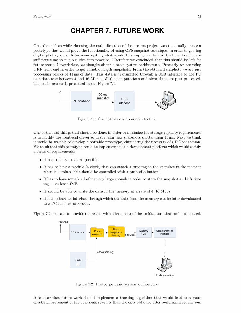
Future work 53
CHAPTER 7. FUTURE WORK
One of our ideas while choosing the main direction of the present project was to actually create aprototype that would prove the functionality of using GPS snapshot techniques in order to geo-tagdigital photographs. After investigating what would this imply, we decided that we do not havesufficient time to put our idea into practice. Therefore we concluded that this should be left forfuture work. Nevertheless, we thought about a basic system architecture. Presently we are usinga RF front-end in order to get variable length snapshots. From the obtained snaphots we are justprocessing blocks of 11 ms of data. This data is transmitted through a USB interface to the PCat a data rate between 4 and 16 Mbps. All the computations and algorithms are post-processed.The basic scheme is presented in the Figure 7.1.
RF front-endUSB
interface
20 ms
snapshot
Figure 7.1: Current basic system architecture
One of the first things that should be done, in order to minimize the storage capacity requirementsis to modify the front-end driver so that it can take snapshots shorter than 11 ms. Next we thinkit would be feasible to develop a portable prototype, eliminating the necessity of a PC connection.We think that this prototype could be implemented on a development platform which would satisfya series of requirements:
• It has to be as small as possible
• It has to have a module (a clock) that can attach a time tag to the snapshot in the momentwhen it is taken (this should be controlled with a push of a button)
• It has to have some kind of memory large enough in order to store the snapshot and it’s timetag — at least 1MB
• It should be able to write the data in the memory at a rate of 4–16 Mbps
• It has to have an interface through which the data from the memory can be later downloadedto a PC for post-processing
Figure 7.2 is meant to provide the reader with a basic idea of the architecture that could be created.
Antenna
Post-processing
RF front-end4-16Mbps
20 ms
snapshot
Clock
Attach time tag
20 ms
snapshot +
time tag
Communication
interface
Memory
1MB
Figure 7.2: Prototype basic system architecture
It is clear that future work should implement a tracking algorithm that would lead to a moredrastic improvement of the positioning results than the ones obtained after performing acquisition.

If such an algorithm would be implemented, the next step would be to check the effects of thepseudo-range corrections while using snapshot techniques. One other issue that has to be dealtwith in future work is implementing a proper working Doppler positioning algorithm. The majorpart of these two algorithms are already done, their bodies have been programmed, therefore, wefeel that we did not succeed to properly deal with this two issues also due to lack of time.
This being a student project, its main purposes are academical. We just wanted to provide aproof-of-concept. Consequently, we did not deal that much with the optimization of our software.We consider this also to be a significant future work. One way to optimize the code and shortenthe execution time is to program the algorithms in another programming language such as C++instead of using Matlab. Matlab is a very good didactic tool but it can not compete with C++when it comes to building a commercial mass-market application. Another idea that we hadthat might optimize the execution time of the real-life application is that, due to the convergencecapabilities of the positioning algorithms, we might be able to eliminate redundant snapshots. Forexample if two or more snapshots are taken in a very short interval of time, 20 s, say, we can storeand use only one of them, taking into account that the user could not have moved that far awayfrom the initial position. We imagine an application meant for digital photography, therefore mostof the snapshots will be taken while standing still.

APPENDICES

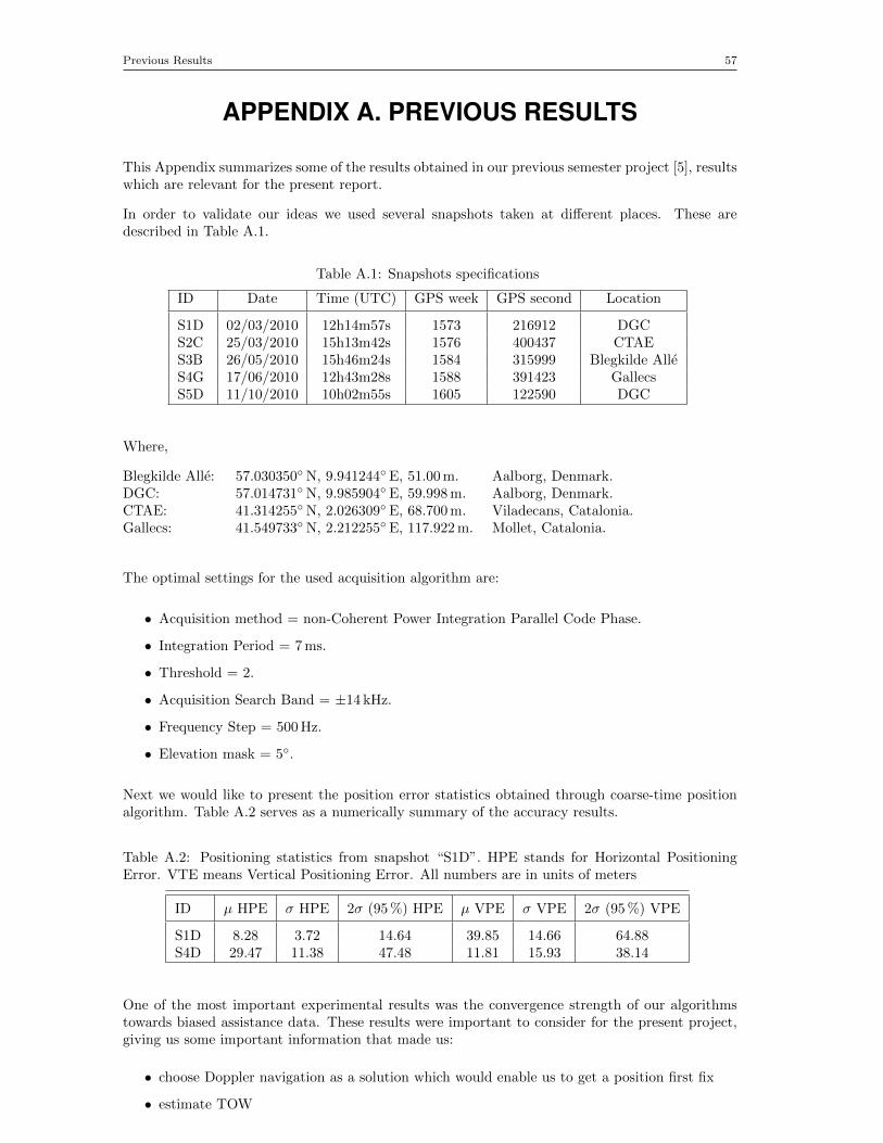
Previous Results 57
APPENDIX A. PREVIOUS RESULTS
This Appendix summarizes some of the results obtained in our previous semester project [5], resultswhich are relevant for the present report.
In order to validate our ideas we used several snapshots taken at different places. These aredescribed in Table A.1.
Table A.1: Snapshots specifications
ID Date Time (UTC) GPS week GPS second Location
S1D 02/03/2010 12h14m57s 1573 216912 DGCS2C 25/03/2010 15h13m42s 1576 400437 CTAES3B 26/05/2010 15h46m24s 1584 315999 Blegkilde AlleS4G 17/06/2010 12h43m28s 1588 391423 GallecsS5D 11/10/2010 10h02m55s 1605 122590 DGC
Where,
Blegkilde Alle: 57.030350◦N, 9.941244◦ E, 51.00 m. Aalborg, Denmark.DGC: 57.014731◦N, 9.985904◦ E, 59.998 m. Aalborg, Denmark.CTAE: 41.314255◦N, 2.026309◦ E, 68.700 m. Viladecans, Catalonia.Gallecs: 41.549733◦N, 2.212255◦ E, 117.922 m. Mollet, Catalonia.
The optimal settings for the used acquisition algorithm are:
• Acquisition method = non-Coherent Power Integration Parallel Code Phase.
• Integration Period = 7 ms.
• Threshold = 2.
• Acquisition Search Band = ±14 kHz.
• Frequency Step = 500 Hz.
• Elevation mask = 5◦.
Next we would like to present the position error statistics obtained through coarse-time positionalgorithm. Table A.2 serves as a numerically summary of the accuracy results.
Table A.2: Positioning statistics from snapshot “S1D”. HPE stands for Horizontal PositioningError. VTE means Vertical Positioning Error. All numbers are in units of meters
ID µ HPE σ HPE 2σ (95 %) HPE µ VPE σ VPE 2σ (95 %) VPE
S1D 8.28 3.72 14.64 39.85 14.66 64.88S4D 29.47 11.38 47.48 11.81 15.93 38.14
One of the most important experimental results was the convergence strength of our algorithmstowards biased assistance data. These results were important to consider for the present project,giving us some important information that made us:
• choose Doppler navigation as a solution which would enable us to get a position first fix
• estimate TOW
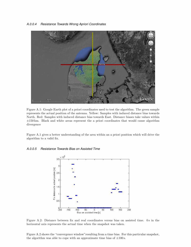
A.0.0.4 Resistance Towards Wrong Apriori Coordinates
Figure A.1: Google Earth plot of a priori coordinates used to test the algorithm. The green samplerepresents the actual position of the antenna. Yellow: Samples with induced distance bias towardsNorth. Red: Samples with induced distance bias towards East. Distance biases take values within±150 km. Black and white areas represent the a priori coordinates that would cause algorithmdivergence
Figure A.1 gives a better understanding of the area within an a priori position which will drive thealgorithm to a valid fix.
A.0.0.5 Resistance Towards Bias on Assisted Time
Figure A.2: Distance between fix and real coordinates versus bias on assisted time. 0 s in thehorizontal axis represents the actual time when the snapshot was taken.
Figure A.2 shows the “convergence window”resulting from a time bias. For this particular snapshot,the algorithm was able to cope with an approximate time bias of ±100 s.
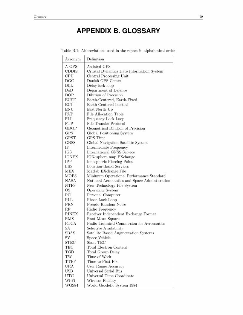
Glossary 59
APPENDIX B. GLOSSARY
Table B.1: Abbreviations used in the report in alphabetical order
Acronym Definition
A-GPS Assisted GPSCDDIS Crustal Dynamics Date Information SystemCPU Central Processing UnitDGC Danish GPS CenterDLL Delay lock loopDoD Department of DefenceDOP Dilution of PrecisionECEF Earth-Centered, Earth-FixedECI Earth-Centered InertialENU East North UpFAT File Allocation TableFLL Frequency Lock LoopFTP File Transfer ProtocolGDOP Geometrical Dilution of PrecisionGPS Global Positioning SystemGPST GPS TimeGNSS Global Navigation Satellite SystemIF Intermediate FrequencyIGS International GNSS ServiceIONEX IONosphere map EXchangeIPP Ionospheric Piercing PointLBS Location-Based ServicesMEX Matlab EXchange FileMOPS Minimum Operational Performance StandardNASA National Aeronautics and Space AdministrationNTFS New Technology File SystemOS Operating SystemPC Personal ComputerPLL Phase Lock LoopPRN Pseudo-Random NoiseRF Radio FrequencyRINEX Receiver Independent Exchange FormatRMS Root Mean SquareRTCA Radio Technical Commission for AeronauticsSA Selective AvailabilitySBAS Satellite Based Augmentation SystemsSV Space VehicleSTEC Slant TECTEC Total Electron ContentTGD Total Group DelayTW Time of WeekTTFF Time to First FixURA User Range AccuracyUSB Universal Serial BusUTC Universal Time CoordinateWi-Fi Wireless FidelityWGS84 World Geodetic System 1984

Group Dynamics 61
APPENDIX C. GROUP DYNAMICS
For this semester project our group was made up just from two students: Oriol Badia Sole fromBarcelona and Tudor Iacobescu from Romania. Both of us have similar education background,both having a bachelor degree in telecommunication engineering.
Because of the fact that we knew each other and worked together in the previous semesters aswell, it was easier to get along from a personal point of view. Both of us have more or less thesame mentality when work and study is concerned, so work cooperation was good this semester.Since the beginning of the semester we decided that we should have daily meetings. With someexceptions we respected this. Working together daily made communication between us easier.Another reason why we decided to work together every day is that in this way we could avoidredundant work. Being in the same room, it was very easy for each of us to communicate his workplan of the day. Basically we tried every morning to explain to each other what each of us wantedto do. After we agreed on the work plan of the day, we actually started work. Of course objectionscame up, but we succeeded to discuss in a calm way and work all our problems out. Besides thesedaily meetings we also tried to have a reflection and planning meeting each week. The purpose ofthis was to see what was accomplished each week, explain certain aspects to one another and planfor the next stage of the project work.
From a more technical point of view, we shared our work and data through Smart SVN versioncontrol. This software also acts like a means of data backup. But still after each modification inthe code or the report we still made verbal notifications to each other, in order to avoid conflicterrors which are very common while using version control.
As it is expected in every group of people, however small it may be, small conflicts and quarrelsalso took place. But in the end we think these were solved in a calm and mature way, leaving moretime to concentrate on the study aspect of group work instead of the personal one.
With this project we will conclude our work together. As a reflection on group dynamics, not onlyin this semester, but throughout our entire studies, we feel we worked very good together.

Group Dynamics 63
BIBLIOGRAPHY
[1] Wireless Innovation Forum. Introduction to sdr. ”http://www.wirelessinnovation.org”,”unpublished manuscript”.
[2] Minimum operational performance standards for global positioning system/wide area aug-mentation system airborne equipment. Technical report, 2006. DO-229C.
[3] GPS Joint Program Office. Is-gps-200 revision d - interface specification - navstar gps spacesegment/navigation user interfaces. Technical report, 2004. ”http://www.navcen.uscg.gov/gps/geninfo/IS-GPS-200D.pdf”.
[4] Elliott D. Kaplan and Christopher Hegarty. Understanding GPS: Principles and Applications.Royal Aircraft Establishment.
[5] Oriol Badia and Tudor Iacobescu. Gps snapshot techniques. Technical report, Danish GPSCenter, AAU.
[6] Kai Borre and Darius Plausinaitis. Reconfigurable gnss receivers. ”http://kom.aau.dk/project/softgps/GNSS_SummerSchool_DGC.pdf”, 2007.
[7] Bradford W. Parkinson and James J. Spilker Jr. Global Positioning System: Theory andApplications, volume I. American Institute of Aeronautics and Astronautics, Inc., 1996. ISBN:1-56347-106-X.
[8] M. Hernandez-Pajares, J.M. Juan Zornoza, and J. Sanz Subirana. GPS data processing: codeand phase: Algorithms, Techniques and Recipes. Edicions UPC, 1st edition (english) edition,2005. ISBN 84-932230-5-0.
[9] Gilbert Strang and Kai Borre. Linear Algebra, Geodesy and GPS. Wellesley-Cambridge Press,1997.
[10] Kai Borre, Dennis M. Akos, Nicolaj Bertelsen, Peter Rinder, and Søren Holdt Jensen. ASoftware-defined GPS and Galileo receiver: A single-frequency approach. Birkhauser, 2007.ISBN-10 0-8176-4390-7.
[11] Stefan Schaer, Werner Gurtner, and Joachim Feltens. Ionex: The ionosphere map exchangeformat. Technical report, 1998. Version 1.0.
[12] Xin-Xiang JIN. Theory of Carrier Adjusted DGPS Psitioning Approach and Some Experi-mental Results. PhD thesis, Delft University, 1996.
[13] J.G. Walker. Continuos Whole-Earth Coverage by Circular-Orbit Satellite Patterns. ArtechHouse Publishers, 2th edition edition, 2005. ISBN-10 / ASIN: 1580538940.
[14] Frank van Diggelen. A-GPS: Assisted GPS, GNSS, and SBAS. Boston: Artech House Pub-lishers, 2009. ISBN 1596933747.
[15] Inc. John Wiley & Sons. Gps1a: A software-defined gnss receiver. Technical report, 2004.ISBN 0-471-38154-3.
[16] Cypress Semiconductor Corporation. EZ-USB FX2LPTM USB Microcontroller, 200104. Doc-ument: 38-08032 Revised September 23, 2010.
[17] SiGE. SE4110L GPS Receiver IC.
[18] Jan Alvestad. Solar terrestrial activity report. ”http://www.solen.info/solar/solcycle.html”.
[19] A. D. Andrews. Solar maximmum events 22 march to 31 may 2000. Irish AstronomicalJournal, 27(2), 160-232. Provided by the NASA Astrophysics Data System.