Embed Size (px)
Citation preview

Electricity Forward Curves with Thin Granularity
Mercati Energetici e Metodi Quantitativi: un ponte tra universitá e
aziende
Ruggero Caldana (presenter), Gianluca Fusai, Andrea Roncoroni
Accenture SPA, Milan - Italy
Padova, October 13, 2016

Curve
HPFC de�nition
The hourly price forward curve (HPFC) quoted in a given market at a day
t is a mathematical function ft (T , h) associating to each day T in the
future a price for the commitment to deliver one megawatt-hour for a
speci�c hour h of that speci�c day, i.e. the term structure of electricity
forward prices as quoted with hourly granularity across the maturity
dimension.
Academic and industrial relevance:
1 Marking energy portfolios to market quotes (Teixeira Lopes (2007)),2 Calibrating arbitrage models (Islyaev-Date (2015)),3 Analyzing risk premia (Frestad-Benth-Koekebakker (2010)),4 Conceiving and testing prop trading rules (Furio-Lucia (2009)),5 Consumption optimization in energy-intensive processes (Lima (2015)),6 Real option based physical asset valuation (Nasakkalaa-Fleten (2005)).
Ruggero Caldana (presenter), Gianluca Fusai, Andrea Roncoroni Electricity Forward Curves with Thin Granularity

Literature
Fleten-Lemming (2003) benchmark parametric curve �tting to a
proprietary equilibrium model.
Koekkebakker-OsAdland (2004) and Benth-Koekebakker-Ollmar (2007)
combine seasonalities with splines and minimize curve convexity.
Borak and Weron (2008) propose a parsimonious, smooth, and seasonal
forward curve.
Hildmann-Ka�e-Anderson (2012) model hourly prices.
Paraschiv-Fleten-Schurle (2015) extend Benth et al. (2007) method to
account for hourly granularity and weather-linked factors.
Ruggero Caldana (presenter), Gianluca Fusai, Andrea Roncoroni Electricity Forward Curves with Thin Granularity

Issue
We put forward a Rational Constructive De�nition of electricity forward
curve with thin granularity.
Constructive = Algorithmic.
Rational = Complying with 5 desirable properties:
1 Raw price series undergo a �ltering procedure to �nely detect and single
out data outliers;2 Curve shape embeds a comprehensive bundle of periodical patterns
unveiled by past quotes;3 Curve level is jointly consistent to standing baseload and peakload futures
quotations;4 Curve path satis�es regularity properties: smoothness, monotonicity
preservation, cross-sectional stability, time localness (Hagan-West (2006));5 Forward estimate quality is assessed through dedicated empirical tests.
Ruggero Caldana (presenter), Gianluca Fusai, Andrea Roncoroni Electricity Forward Curves with Thin Granularity

Example of futures market data
Figure: Futures market data from EEX, November 7, 2013. Settlement prices
are given in Eur/MWh.
Jan14 Apr14 Jul14 Oct14 Feb15 May15 Aug15 Dec1525
30
35
40
45
50
55
60
BaseloadPeakload
Ruggero Caldana (presenter), Gianluca Fusai, Andrea Roncoroni Electricity Forward Curves with Thin Granularity

Idea
1 Reduction to forward kernel:
obsF =
1
τ e − τ b
∫ τe
τbft(u)du → ft(·) → all prices.
2 Construction of forward kernel:
APT : Arbitrage-free spot model dS (t) → ft(u) := E∗t [S(u)];
Our method is dynamic model independent:
ft(u) := Λt(u) + εt(u) + ϕt (u) ,
Λ → Periodical patterns (Historical information),
εt → Calibration to baseload forwards (Risk-neutral information),
ϕt → Calibration of peakload forwards (Risk-neutral information).
Ruggero Caldana (presenter), Gianluca Fusai, Andrea Roncoroni Electricity Forward Curves with Thin Granularity

Construction
Ruggero Caldana (presenter), Gianluca Fusai, Andrea Roncoroni Electricity Forward Curves with Thin Granularity

Data
Market: EPEX Spot SE and EEX Power Derivatives;
Data:
〈Spot → 24×2,525 obs. [Jan. 1, 2009 - Nov. 27, 2015];
Forward → baseload and peakload, on Nov. 27, 2015.
Filtering:
Aug09 Dec10 May12 Sep13 Feb15-60
-40
-20
0
20
40
60
80
100Filtered pricesFilter for preprocessingIdentified Outliers
Aug09 Dec10 May12 Sep13 Feb150
10
20
30
40
50
60
70
80
90Daily priceFiltered daily trend
Ruggero Caldana (presenter), Gianluca Fusai, Andrea Roncoroni Electricity Forward Curves with Thin Granularity

Analysis of predictable components
A seasonality function for the German market
Λ(u) = a cos
(2π
365u + b
)︸ ︷︷ ︸
Long term (LT)
+7∑
j=1
cj1(u ∈ dayj )
︸ ︷︷ ︸Weekly (W)
+24∑h=1
4∑l=1
dh,l1(u ∈ hourh ∩ u ∈ Cl )︸ ︷︷ ︸Daily (D)
,
where:
u ∈ R, and a, cj , dh,l ∈ R ∀h, j, k, l and b ∈ [0, 2π].
dayj for j = 1, . . . , 7 := the set of points in the jth day of the week (i.e. j = 1 refer to
Sunday . . . , j = 7 refer to Saturday).
hourh, h = 1, . . . , 24, := the set of points in the hth hour of a day.
C1 := working days in the cold season (from October to March).
C2 := non-working days in the cold season (from October to March).
C3 := working days in the warm season (from April to September).
C4 := non-working days in the warm season (from April to September).∑24h=1 dh,l = 0, l = 1, . . . , 4.
Ruggero Caldana (presenter), Gianluca Fusai, Andrea Roncoroni Electricity Forward Curves with Thin Granularity
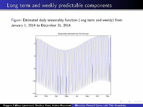
Long term and weekly predictable components
Figure: Estimated daily seasonality function (long term and weekly) from
January 1, 2014 to December 31, 2014.
Jan Feb Apr May Jul Sep Oct Dec−15
−10
−5
0
5
Seasonality estimated over the first year
Ruggero Caldana (presenter), Gianluca Fusai, Andrea Roncoroni Electricity Forward Curves with Thin Granularity

Daily shape
Figure: Hourly seasonality pro�le: variables dh,l are plotted for h = 1, . . . , 24.
Working days - cold season Non-working days - cold season
2 4 6 8 10 12 14 16 18 20 22 24−20
−15
−10
−5
0
5
10
15
20
Hourly profile cluster C1
2 4 6 8 10 12 14 16 18 20 22 24−20
−15
−10
−5
0
5
10
15
20
Hourly profile cluster C2
Working days - warm season Non-working days - warm season
2 4 6 8 10 12 14 16 18 20 22 24−20
−15
−10
−5
0
5
10
15
20
Hourly profile cluster C3
2 4 6 8 10 12 14 16 18 20 22 24−20
−15
−10
−5
0
5
10
15
20
Hourly profile cluster C4
Ruggero Caldana (presenter), Gianluca Fusai, Andrea Roncoroni Electricity Forward Curves with Thin Granularity

Market consistency adjusment
Baseload consistency adjusment
We de�ne ε through the monotone convex spline put forward in (Hagan
West, 2006) that guarantees
1 Consistency to baseload futures.
2 Positivity of ε.
3 Continuity of ε.
4 Monotonicity of ε.
Peakload consistency adjustment
Peakload consistency adjustment ϕ is obtained through a constant
pathwise shift on peak and o�-peak hours for workdays only. The
adjustment is constrained to not a�ect baseload consistency.
Ruggero Caldana (presenter), Gianluca Fusai, Andrea Roncoroni Electricity Forward Curves with Thin Granularity

Curve
Dec15 Jan16 Mar16 Apr16 Jun16 Aug16 Sep16 Nov160
10
20
30
40
50
60Hourly PriceBaseloadPeakload
Dec15 Jan16
5
10
15
20
25
30
35
40
45
50
55 Hourly PriceBaseloadPeakload
Ruggero Caldana (presenter), Gianluca Fusai, Andrea Roncoroni Electricity Forward Curves with Thin Granularity

8. Curve Decomposition
Dec15 Jan16 Mar16 Apr16 Jun16 Aug16 Sep16 Nov16-20
-10
0
10
20
30
40LambdaEpsilonPhi
Dec15 Jan16
-15
-10
-5
0
5
10
15
20
25
30
35 LambdaEpsilonPhi
Ruggero Caldana (presenter), Gianluca Fusai, Andrea Roncoroni Electricity Forward Curves with Thin Granularity

Localness
Cross-sectional localness = Any change occurring on whatever segmented
baseload quote (e.g., spot price down by 20 EUR/MWh from Feb. 28,
2013 quote of 53.96) exclusively a�ects curve estimate on the
corresponding delivery interval as well as on the two adjacent ones.
Maximum smoothness (Bent et al. (2007)) Our model
Mar13 Jun13 Sep13 Jan14 Apr14 Jul14 Oct1410
15
20
25
30
35
40
45
50
55
6028 February 201328 February 2013 Stressed
Mar13 Jun13 Sep13 Jan14 Apr14 Jul14 Oct1415
20
25
30
35
40
45
50
5528 February 201328 February 2013 Stressed
Ruggero Caldana (presenter), Gianluca Fusai, Andrea Roncoroni Electricity Forward Curves with Thin Granularity

Stability
Time stability = Small perturbations in input data (e.g.,
26-27-28/2/2013) entail a slight curve variation.
Maximum smoothness Interpolation Our model
Mar13 Jun13 Sep13 Jan14 Apr14 Jul14 Oct140
10
20
30
40
50
60
7026 February 201327 February 201328 February 2013
Mar13 Jun13 Sep13 Jan14 Apr14 Jul14 Oct1425
30
35
40
45
50
55
60
6526 February 201327 February 201328 February 2013
Ruggero Caldana (presenter), Gianluca Fusai, Andrea Roncoroni Electricity Forward Curves with Thin Granularity

Fit Quality I
Futures prices risk premia
Futures prices incorporate risk premia and thus the realized spot price
cannot be used as benchmark to assess the HPFC �t quality.
We need to build �ctitious futures quotes that can be compared to
realized day-ahead price.
Ruggero Caldana (presenter), Gianluca Fusai, Andrea Roncoroni Electricity Forward Curves with Thin Granularity

Fit Quality II
Figure: Backtesting the �t quality for t0 = September 1, 2012. First, we
calibrate the seasonality function on realized prices preceding t0, and we use
prices following t0 to compute �ctitious futures quotations.
10/24/11 02/01/12 05/11/12 08/19/12 11/27/12 03/07/13 06/15/13
−200
−150
−100
−50
0
50
100
150
200
Realized hourly price
Seasonality estimation before t0 Fictitious futures construction after t0
t0 = 1−Sep−2012
Ruggero Caldana (presenter), Gianluca Fusai, Andrea Roncoroni Electricity Forward Curves with Thin Granularity

Fit Quality III
Testing the quality of forward estimates w.r.t. Benth et al. (2007)'s MSI.
Data: 16 evaluation dates = �rst day in Jan., Apr., Jul. 2010 → 2013.
Prices preceding an evaluation → periodical patterns estimate.
Prices following each evaluationavg→ �ctitious baseloads/peakloads.
Performance index: MAD = 1
24]S∑
T∈S∑
h=1,...,24
∣∣∣f (T , h)− S(T , h)∣∣∣
Output: 2 models×16 dates×3 patterns = 96 MAD �gures.
Main result: our model outperforms benchmark MSI on 34 out of 48
scenarios, which correspond to 70.83% of the sample.
Ruggero Caldana (presenter), Gianluca Fusai, Andrea Roncoroni Electricity Forward Curves with Thin Granularity

Conclusion
Constructive de�nition of forward curve with hourly granularity up.
Curve is jointly consistent to risk-neutral & historical market information.
Curve paths are smooth, monotonic, cross-sectionally stable, time local.
Backtesting analysis w.r.t. benchmark model of Benth et al. (2007).
What's next?
Analyzing the interplay between HPFC cross-sectional granularity and the
underlying market price of risk.
Adjustments to cope with the great variety of commodity price dynamics
featuring periodical patterns (e.g., natural gas, agriculturals)
Ruggero Caldana (presenter), Gianluca Fusai, Andrea Roncoroni Electricity Forward Curves with Thin Granularity

Thanks for your attention!
Ruggero Caldana (presenter), Gianluca Fusai, Andrea Roncoroni Electricity Forward Curves with Thin Granularity