Embed Size (px)
Citation preview
Multi–scale modeling of textile
composites
Thiam Wai Chua
MT 10.19
Master of Science graduation project report
January, 2011
Supervisors:dr.ir. Varvara Kouznetsovadr.ir. Wouter Wilsonprof.dr.ir. Marc Geers
Mechanics of MaterialsComputational and Experimental MechanicsDepartment of Mechanical EngineeringTechnische Universiteit Eindhoven
Abstract
In this project, a coupled multi–scale framework is developed for analysis of fiber–reinforced composites. The developed framework is a versatile tool to study the mechan-ical behavior at the macroscopic level and simultaneously the impact of the mechanicalbehavior from the microscopic level to macroscopic level. In the framework, the macro-scopic material constitutive behavior at each integration point is obtained through theunderlying microscopic composite structure. Abaqus subroutines are used to link themicroscopic level to the macroscopic level structural analyses and vice versa. The fo-cus of this project is to document and present the development and added value of theframework to the analysis of the textile composites. Thus, the quantitative comparisonbetween the analysis results and experimental data has not been attempted. However,the qualitative comparison has been made successfully to verify the correctness of theframework functionality. Multi–scale analyses on the tensile test of a cross–ply laminateand compression test on a notched quasi–isotropic laminate are performed in order toillustrate and demonstrate the power and utility of the framework. This framework canbe seen as a powerful and useful tool for future engineering analysis and design of com-posite structure due to its flexibility to apply on many textile composites which hardlyto be achieved using other analytical approaches. Thus, engineers enable to utilize thisframework at the beginning stage of the composite structures design and developmentfor the savings of cost and time.
Keywords: coupled multi–scale analysis, composites, Abaqus.
i
Contents
Abstract i
1 Introduction 1
1.1 Composite aerospace landing gear structures . . . . . . . . . . . . . . . . 1
1.2 Textile composites . . . . . . . . . . . . . . . . . . . . . . . . . . . . . . 2
1.3 Modeling approaches for textile composites . . . . . . . . . . . . . . . . . 2
1.4 Motivation . . . . . . . . . . . . . . . . . . . . . . . . . . . . . . . . . . . 4
1.5 Scope and outline . . . . . . . . . . . . . . . . . . . . . . . . . . . . . . . 4
2 Multi–scale modeling framework description 6
2.1 Basic hypotheses . . . . . . . . . . . . . . . . . . . . . . . . . . . . . . . 6
2.2 Microscopic level boundary value problem . . . . . . . . . . . . . . . . . 7
2.3 Macro–micro levels coupling . . . . . . . . . . . . . . . . . . . . . . . . . 9
2.3.1 Deformation . . . . . . . . . . . . . . . . . . . . . . . . . . . . . . 9
2.3.2 Stress . . . . . . . . . . . . . . . . . . . . . . . . . . . . . . . . . 10
2.3.3 Internal work . . . . . . . . . . . . . . . . . . . . . . . . . . . . . 11
2.4 Numerical implementation . . . . . . . . . . . . . . . . . . . . . . . . . . 11
2.4.1 Micro–structure boundary value problem . . . . . . . . . . . . . . 11
2.4.2 Macroscopic stress . . . . . . . . . . . . . . . . . . . . . . . . . . 12
2.4.3 Macroscopic tangent stiffness . . . . . . . . . . . . . . . . . . . . 12
2.5 Modeling framework implementation using Abaqus . . . . . . . . . . . . 13
2.6 Modeling framework verification . . . . . . . . . . . . . . . . . . . . . . . 13
3 Micro–structural modeling 19
3.1 Textile and non–crimp composite models . . . . . . . . . . . . . . . . . . 19
3.2 Material properties . . . . . . . . . . . . . . . . . . . . . . . . . . . . . . 20
3.3 Finite element model . . . . . . . . . . . . . . . . . . . . . . . . . . . . . 21
3.4 Microscopic level analyses . . . . . . . . . . . . . . . . . . . . . . . . . . 22
3.4.1 Tension test . . . . . . . . . . . . . . . . . . . . . . . . . . . . . . 25
3.4.1.1 Uniaxial tension . . . . . . . . . . . . . . . . . . . . . . 25
3.4.1.2 Biaxial tension . . . . . . . . . . . . . . . . . . . . . . . 25
3.4.2 Compression test . . . . . . . . . . . . . . . . . . . . . . . . . . . 26
3.4.3 Shear test . . . . . . . . . . . . . . . . . . . . . . . . . . . . . . . 28
4 Application of the multi–scale modeling framework 31
4.1 Tensile test on a cross–ply laminate . . . . . . . . . . . . . . . . . . . . . 31
4.2 Compression test on a notched quasi–isotropic laminate . . . . . . . . . . 36
ii
Contents iii
5 Conclusions and recommendations 475.1 Conclusions . . . . . . . . . . . . . . . . . . . . . . . . . . . . . . . . . . 475.2 Recommendations for future work . . . . . . . . . . . . . . . . . . . . . . 48
5.2.1 Multi–scale modeling framework . . . . . . . . . . . . . . . . . . . 485.2.2 Micro–structural modeling . . . . . . . . . . . . . . . . . . . . . . 495.2.3 Application of the multi–scale modeling framework . . . . . . . . 50
Bibliography 51
Appendices 58
A Literature survey 59
B Macro–micro levels coupling 64
C Microscopic level boundary value problem 67
D Macroscopic stress calculation 70
E Condensation of the microscopic stiffness 74
F Consistent tangent stiffness for the Kirchhoff stress tensor 75
G Total matrix of the reduced stiffness matrix 78
H Incremental–iterative multi–scale modeling approach 80
I Multi–scale analyses of unidirectional fiber reinforced composite 82
Chapter 1
Introduction
1.1 Composite aerospace landing gear structures
Composite materials are very attractive to engineers because of their advantages com-pared with many conventional engineering materials (e.g. steel, aluminum, metallic al-loys, etc.), such as high strength–to–weight ratio, dimensional stability, superior corrosionresistance and relatively high impact resistance [62]. Besides that, the multi–phase andmulti–layer composites can be tailored through different fiber directions, lamina thick-nesses and stacking sequences for specific design requirements.
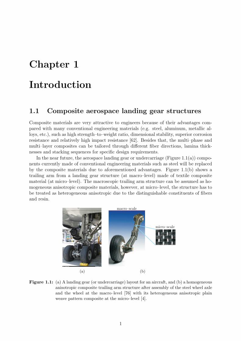
In the near future, the aerospace landing gear or undercarriage (Figure 1.1(a)) compo-nents currently made of conventional engineering materials such as steel will be replacedby the composite materials due to aforementioned advantages. Figure 1.1(b) shows atrailing arm from a landing gear structure (at macro–level) made of textile compositematerial (at micro–level). The macroscopic trailing arm structure can be assumed as ho-mogeneous anisotropic composite materials, however, at micro–level, the structure has tobe treated as heterogeneous anisotropic due to the distinguishable constituents of fibersand resin.
(a)
macro–scale
micro–scale
(b)
Figure 1.1: (a) A landing gear (or undercarriage) layout for an aircraft, and (b) a homogeneousanisotropic composite trailing arm structure after assembly of the steel wheel axleand the wheel at the macro–level [76] with its heterogeneous anisotropic plainweave pattern composite at the micro–level [4].
1
2 Chapter 1
1.2 Textile composites
Textile composites (also know as fabric composites) are a relatively new class of advancedcomposites [89]. They offer advantages and opportunities for designing and tailoringthe textile structures for aerospace structures in order to meet the strict design andfunctional requirements. For instance, they provide an excellent impact resistance dueto the bidirectional fiber configuration compared with the conventional unidirectionalfiber configuration in a lamina [83]. In addition, the production of geometrically complextextile composites becomes relatively efficient and cost–effective due to the significantdevelopment of the weaving manufacturing technology based on the loom technique [89].Kamiya et al. [32] reviewed some of the recent advanced techniques in the fabrication andthe design of textile preforms. Some of the applications of the advanced textile compositesin aircraft, marine, automobiles, civil infrastructures as well as medical prosthesis werereviewed by Mouritz et al. [53].
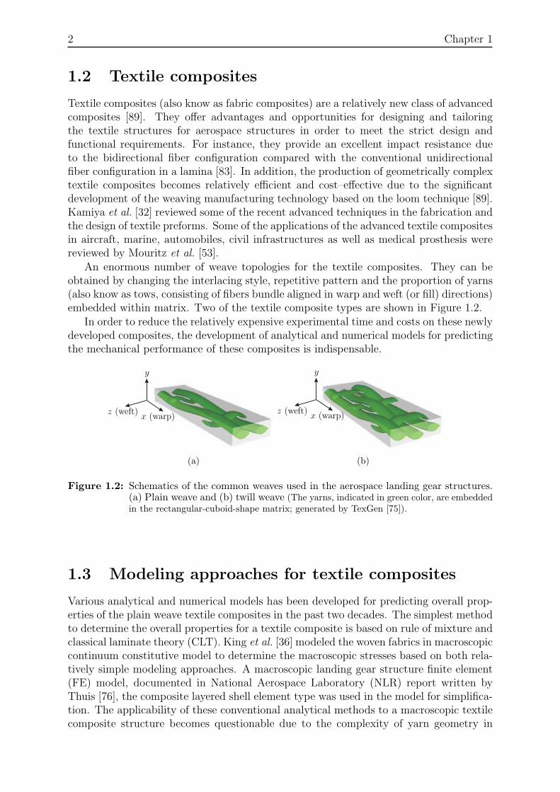
An enormous number of weave topologies for the textile composites. They can beobtained by changing the interlacing style, repetitive pattern and the proportion of yarns(also know as tows, consisting of fibers bundle aligned in warp and weft (or fill) directions)embedded within matrix. Two of the textile composite types are shown in Figure 1.2.
In order to reduce the relatively expensive experimental time and costs on these newlydeveloped composites, the development of analytical and numerical models for predictingthe mechanical performance of these composites is indispensable.
x (warp)
y
z (weft)
(a)
x (warp)
y
z (weft)
(b)
Figure 1.2: Schematics of the common weaves used in the aerospace landing gear structures.(a) Plain weave and (b) twill weave (The yarns, indicated in green color, are embeddedin the rectangular-cuboid-shape matrix; generated by TexGen [75]).
1.3 Modeling approaches for textile composites
Various analytical and numerical models has been developed for predicting overall prop-erties of the plain weave textile composites in the past two decades. The simplest methodto determine the overall properties for a textile composite is based on rule of mixture andclassical laminate theory (CLT). King et al. [36] modeled the woven fabrics in macroscopiccontinuum constitutive model to determine the macroscopic stresses based on both rela-tively simple modeling approaches. A macroscopic landing gear structure finite element(FE) model, documented in National Aerospace Laboratory (NLR) report written byThuis [76], the composite layered shell element type was used in the model for simplifica-tion. The applicability of these conventional analytical methods to a macroscopic textilecomposite structure becomes questionable due to the complexity of yarn geometry in
Introduction 3
three–dimensional (3D) space at microscopic level and unable to describe the mechanicalbehavior of a composite microscopically.
A relatively sophisticated one–dimensional (1D) mosaic model developed by Ishikawaand Chou [27] for the plain weave textile composite. The major drawback of this modelis that the yarns continuity is not taken into account. To improve on this, Ishikawaand Chou [29] proposed the crimp model as an extension of their mosaic model. Thismodel has taken into account the continuity and the undulation of yarns, however, onlyalong the loading direction were considered. The transverse yarn undulation and theactual cross–sectional geometry should also be taken into account because they are theimportant factors of the homogenized properties of textile composite.
Next, two two–dimensional (2D) slice array model (SAM) and element array model(EAM) models proposed by Naik and Ganesh [54], for the plain weave textile composites.In these models, the continuity and the undulation of yarns in warp and weft directionsas well as the presence of the gap between adjacent yarns were considered. The differentmaterials and geometrical properties of warp and weft yarns can be modeled.
In order to extend to the 3D analysis and to include the detailed geometrical descrip-tions of the yarns, the method of cell partition has been developed by many researchers( [31,70,71,79]). Through this method, the representative cell is discritized into subcells,where the effective properties of each subcell are obtained.
The limitation of the aforementioned analytical methods were developed specificallyapplied on one type of the textile composite. Thus, they do not offer flexibility to beapplied on other textile composite types, i.e. the analytical methods need to be re–modeled for each textile composite. Due to this consequence, a relatively flexible analysisapproach is needed to analyze on any textile composite without the necessity of re–modeling on the analysis approach.
In recent years, due to the advancement of structural and material modeling tech-nology, a relatively accurate geometrical textile composites models have been developedthrough computer–aided engineering (CAE) and textile geometric modeling software,such as WiseTex [82], TechText CAD [24] and TexGen [63]. As a result, the analyticaltextile model can be circumvented. Enormous number of research papers are availableregarding the geometric modeling using this approach and numerical analysis thereof( [3, 34, 40, 59,64, 65,84,87,88, 93]).
By taking the advantage of FE method and the advancement of CAE and textilegeometric modeling software, an analysis approach for performing the analysis which linkthe macroscopic and microscopic structures can be developed. The FE analysis approachis known as global/local method, it was developed by Whitcomb [85]. This approach hasbeen further implemented by Srirengan et al. [66] and Xu et al. [90] for the 3D stress anal-ysis of the textile composite structures and further improved by Whitcomb et al. [86], whoused homogenized engineering material properties to accelerate the global stress analysisfor the textile composites. Generally, a global FE analysis was performed on a globalregion with the global coarse finite elements, followed by a detailed local FE analysisperformed in a local region with the independent 3D local fine finite elements. However,the main drawback of this approach is that the local level mechanical mechanisms canonly be studied on the region of interest (ROI) on global level.
To address this problem, multi–scale computational homogenization for heterogenousmaterials is proposed by Kouznetsova et al. [38,39], Miehe et al. [50], Miehe [48], Moulinecand Suquet [52], Miehe and Koch [49], Michel et al. [46], Feyel and Chaboche [13], Ter-ada et al. [74]. This approach can be used to study the microscopic mechanical phe-
4 Chapter 1
nomenon within a macroscopic structure collectively and it provides a promising multi–scale solution to many engineering materials with heterogeneous microscopic structures,such as metal alloy systems, porous media, polycrystalline materials [16, 37]. Hence, itis reasonable to expect that the multi–scale computational homogenization approach hasthe capability to solve the relatively complex textile composites problems by bridging themacroscopic and microscopic scales.
The multi–scale computational homogenization method as well as the global/localmethod in the textile composites analysis have their own pros and cons. The selectionbetween both methods should be based on the descriptions of a specific engineering prob-lem. The global/local method is essentially a FE analysis through the mesh refinementtechnique on a region of interest (ROI), e.g. crack tips or specific regions with high stressesor strains. Whereas, the multi–scale computational homogenization approach is used op-timally for predicting the macroscopic structure mechanical response with the underlyingmicroscopic structure phenomenon collectively, i.e. the micro–structural phenomenon ateach macroscopic region can be studied in detail. The comprehensive literature survey ofvarious modeling approaches for textile composites can be found in Appendix A.
1.4 Motivation
A numerical analysis framework for predicting the mechanical and physical responses ofcomposite landing gear materials macroscopically and microscopically is indispensablefor improving the structural design and integrity.
Therefore, based on the literature survey on various textile composite analysis ap-proaches as discussed in Section 1.3, the multi–scale computational homogenization ap-proach is utilized in this project, because the micro–structural phenomenon in variousmacroscopic regions can be studied simultaneously for predicting the failure modes at themicroscopic level.
Besides that, another advantage of this approach is its flexibility for adaptation. Forinstance, the overall elastic properties for variation of geometrical parameters (volumefraction, shape, orientations, etc.) of the constituents can be easily performed withoutthe necessity of re–implementing the analysis framework.
Furthermore, this framework has an additional advantage that the material propertiesare defined on the constituent scale, thereby the macroscopic constitutive equation isunnecessary. Thus, the framework can be incorporated into the design and analysisprocess at early stage.
1.5 Scope and outline
The aim of this project is to investigate the applicability of the coupled macro–microcomputational homogenization approach to the analysis of textile composite structures.Hence, the approach is implemented within the FE framework and its power, utility andlimitation are demonstrated.
In chapter 2, the multi–scale computational homogenization approach is introducedin brief. The concise descriptions of the microscopic boundary value problem and micro–macro coupling framework are given. Then, the implementation of the computationalhomogenization within FE framework is briefly discussed. The quantitative compari-son between numerical results with the analytical solutions and experimental data for
Introduction 5
unidirectional fiber–reinforced composite is performed to verify the correctness of theframework.
Next, in chapter 3, the geometric modeling and material properties for the textile andnon–crimp composite representative volume elements (RVE) are presented. The textileand non–crimp RVEs are modeled for the comparison purposes. Then, the analyses onthe RVEs are performed to exemplify the utility of the computational homogenizationapproach at the microscopic level.
In order to illustrate the power and utility of the framework on textile composite,chapter 4 presents the application of the framework on two types of macroscopic structurescoupled with textile RVEs. Firstly, the multi–scale framework is used to analyze themacroscopic laminate [45o/−45o/45o/−45o]S with two different material and geometricalproperties within RVEs to illustrates the flexibility of the framework. Secondly, theanalysis on notched quasi–isotropic laminate [45◦/0◦/ − 45◦/90◦]S to demonstrate thecapabilities of the framework to analyze a relatively complex macroscopic structure.
Finally, in chapter 5, the limitation of the framework is discussed. Thus, severalsolutions are recommended in order to reduce the computational time and cost of theframework. Then, the future development of the framework for the benefits of engineerswill be discussed.
Chapter 2
Multi–scale modeling frameworkdescription
In the context of solving macroscopic composite structure problems, computational ho-mogenization is used to obtain the overall macroscopic constitutive response from the un-derlying microscopic heterogenous representative volume element (RVE). The advantageof this approach is that the macroscopic constitutive description can be circumvented,where the constitutive behavior at macroscopic level is determined through the micro-scopic constitutive behavior. In this chapter, the crucial components of the multi–scalecomputational homogenization scheme and its FE implementation within Abaqus aretreated in brief.
2.1 Basic hypotheses
A composite material is assumed to be macroscopically sufficiently homogeneous butmicroscopically inhomogeneous (consist of matrix and bundles of fibers), as schematicallyshown in Figure 2.1. Based on the principle of scale separation, the characteristic wavelength of RVE, `m should be considerably smaller than the wave length of the macroscopicloading or the characteristic size of the macroscopic structure counterpart, `M, as follows
`m � `M, (2.1)
where the subscript “M” and “m” refer to macroscopic and microscopic quantities, re-spectively. Due to the morphology of composite materials in a landing gear structure, theglobal periodicity can be assumed, where the fibers bundle (yarns) pattern is repeated inevery macroscopic point, as shown in Figure 2.2 1.
In the computational homogenization scheme [38], the macroscopic deformation gra-dient tensor, FM is calculated at every macroscopic point, i.e. integration points of afinite element (FE) meshed macrostructure. The FM of a particular macroscopic pointis imposed upon RVE (which is assigned to that macroscopic point) to prescribe its totaldeformation. Upon the solution of the RVE boundary value problem, the macroscopicstress tensor (e.g. macroscopic Cauchy stress tensor, σM ) is obtained through the micro-scopic stress tensor (e.g. microscopic Cauchy stress tensor, σm ) using the RVE volume
1Note that the selected periodic plain weave textile composite as shown in Figure 2.2 is only forillustration and schematic purposes. Several possibilities of the periodic RVE for plain weave textilecomposite exist.
6
Multi–scale modeling framework description 7
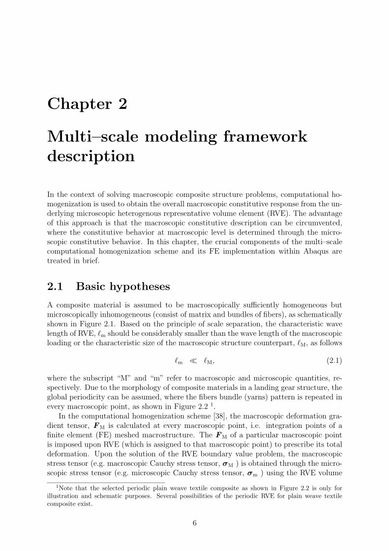
M
Figure 2.1: Continuum macrostructure of a drag brace component and heterogeneous RVE ofa composite at a macroscopic point, M.
weft yarn warp yarn matrix (resin)
Figure 2.2: Schematic representative of a global periodic plain weave textile compositemacrostructure in two dimensional view.
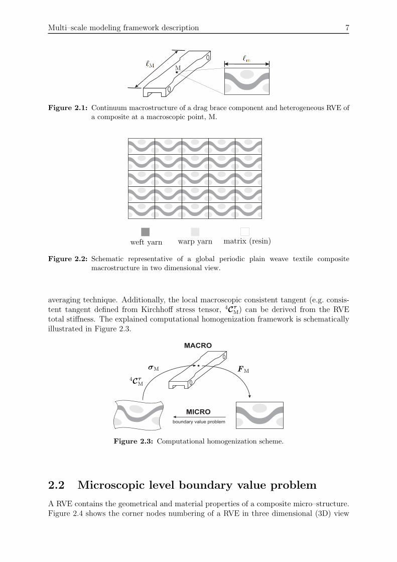
averaging technique. Additionally, the local macroscopic consistent tangent (e.g. consis-tent tangent defined from Kirchhoff stress tensor, 4C
τ
M) can be derived from the RVEtotal stiffness. The explained computational homogenization framework is schematicallyillustrated in Figure 2.3.
boundary value problem
MICRO
MACRO
FMσM
4Cτ
M
Figure 2.3: Computational homogenization scheme.
2.2 Microscopic level boundary value problem
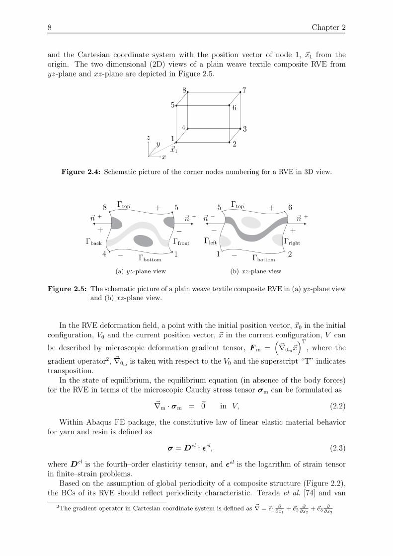
A RVE contains the geometrical and material properties of a composite micro–structure.Figure 2.4 shows the corner nodes numbering of a RVE in three dimensional (3D) view
8 Chapter 2
and the Cartesian coordinate system with the position vector of node 1, ~x1 from theorigin. The two dimensional (2D) views of a plain weave textile composite RVE fromyz-plane and xz-plane are depicted in Figure 2.5.
12
34
5 6
78
x
yz
~x1
Figure 2.4: Schematic picture of the corner nodes numbering for a RVE in 3D view.
+
+
−
−
4 1
58 Γtop
Γbottom
ΓfrontΓback
~n −~n +
(a) yz-plane view
+
+
−
−1 2
5 6Γtop
Γbottom
Γleft Γright
~n − ~n +
(b) xz-plane view
Figure 2.5: The schematic picture of a plain weave textile composite RVE in (a) yz-plane viewand (b) xz-plane view.
In the RVE deformation field, a point with the initial position vector, ~x0 in the initialconfiguration, V0 and the current position vector, ~x in the current configuration, V can
be described by microscopic deformation gradient tensor, Fm =(~∇0m~x
)T, where the
gradient operator2, ~∇0m is taken with respect to the V0 and the superscript “T” indicatestransposition.
In the state of equilibrium, the equilibrium equation (in absence of the body forces)for the RVE in terms of the microscopic Cauchy stress tensor σm can be formulated as
~∇m · σm = ~0 in V, (2.2)
Within Abaqus FE package, the constitutive law of linear elastic material behaviorfor yarn and resin is defined as
σ = Del : εel, (2.3)
where Del is the fourth–order elasticity tensor, and ε
el is the logarithm of strain tensorin finite–strain problems.
Based on the assumption of global periodicity of a composite structure (Figure 2.2),the BCs of its RVE should reflect periodicity characteristic. Terada et al. [74] and van
2The gradient operator in Cartesian coordinate system is defined as ~∇ = ~e1∂
∂x1
+ ~e2∂
∂x2
+ ~e3∂
∂x3
Multi–scale modeling framework description 9
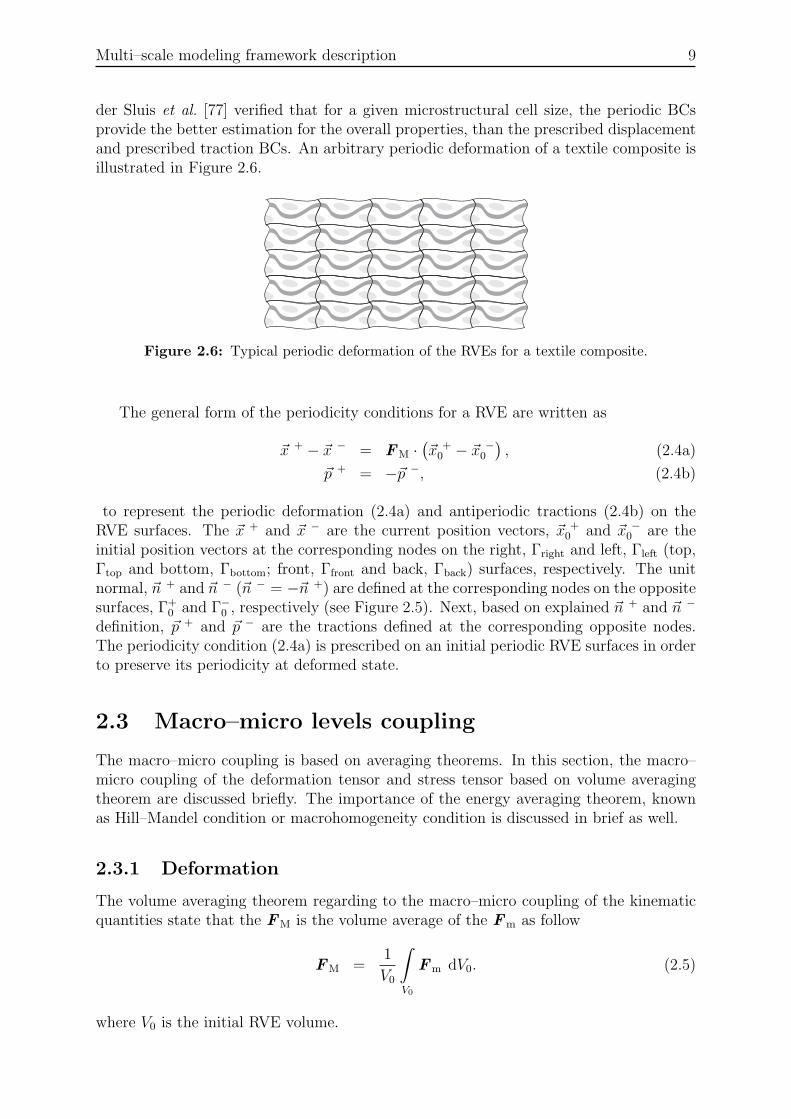
der Sluis et al. [77] verified that for a given microstructural cell size, the periodic BCsprovide the better estimation for the overall properties, than the prescribed displacementand prescribed traction BCs. An arbitrary periodic deformation of a textile composite isillustrated in Figure 2.6.
Figure 2.6: Typical periodic deformation of the RVEs for a textile composite.
The general form of the periodicity conditions for a RVE are written as
~x + − ~x − = FM ·(~x +0 − ~x −
0
), (2.4a)
~p + = −~p −, (2.4b)
to represent the periodic deformation (2.4a) and antiperiodic tractions (2.4b) on theRVE surfaces. The ~x + and ~x − are the current position vectors, ~x +
0 and ~x −
0 are theinitial position vectors at the corresponding nodes on the right, Γright and left, Γleft (top,Γtop and bottom, Γbottom; front, Γfront and back, Γback) surfaces, respectively. The unitnormal, ~n + and ~n − (~n − = −~n +) are defined at the corresponding nodes on the oppositesurfaces, Γ+
0 and Γ−
0 , respectively (see Figure 2.5). Next, based on explained ~n + and ~n −
definition, ~p + and ~p − are the tractions defined at the corresponding opposite nodes.The periodicity condition (2.4a) is prescribed on an initial periodic RVE surfaces in orderto preserve its periodicity at deformed state.
2.3 Macro–micro levels coupling
The macro–micro coupling is based on averaging theorems. In this section, the macro–micro coupling of the deformation tensor and stress tensor based on volume averagingtheorem are discussed briefly. The importance of the energy averaging theorem, knownas Hill–Mandel condition or macrohomogeneity condition is discussed in brief as well.
2.3.1 Deformation
The volume averaging theorem regarding to the macro–micro coupling of the kinematicquantities state that the FM is the volume average of the Fm as follow
FM =1
V0
∫
V0
Fm dV0. (2.5)
where V0 is the initial RVE volume.
10 Chapter 2
According to the divergence (Gauss) theorem
∫
V
~∇ · ~a(~x) dV =
∫
Γ
~n(~x) · ~a(~x) dΓ, (2.6)
where ~a(~x) is a vector function on domain V and ~n(~x) is the outward pointing unit normalto the surface Γ of the domain V . The application of the divergence theorem (2.6) and
Fm =(~∇0m~x
)Tlead to the transformation of (2.5) from volume integral into surface
integral
FM =1
V0
∫
V0
Fm dV0 =1
V0
∫
Γ0
~x~n0 dΓ0. (2.7)
The utilization of the periodic BCs on a RVE leads to the satisfaction of (2.7), as shownin Appendix B.
2.3.2 Stress
The averaging theorem for the first Piola–Kirchhoff stress tensor, P is given as
PM =1
V0
∫
V0
Pm dV0. (2.8)
Next, through applying the relation (with account for microscopic equilibrium equation)
of, ~∇0m ·(P
Tm~x0
)= Pm, the divergence theorem (2.6), and the definition of the micro-
scopic first Piola–Kirchhoff stress vector, ~p = ~n0 · PTm. The PM can be defined on the
RVE surface as follow
PM =1
V0
∫
Γ0
~p~x0 dΓ0. (2.9)
Similarly, the application of the averaging theorem on the σm over current RVE vol-ume, V and the transformation from volume integral to surface integral can be elaboratedas follow
σ∗
M =1
V
∫
Γ
~t~x dΓ. (2.10)
where ~t is the definition of the Cauchy stress vector (~t = ~n · σm).
In the case for kinematic quantities, the nonlinearity between stress measures shouldbe taken with cautiousness, i.e. not all macroscopic stress quantities obtained from thevolume averaging theorem is valid. Therefore, the σM should be defined as
σM =1
det (FM)PM · FT
M. (2.11)
However, in the case of periodic BCs, it can be shown that σ∗
M and σM are equivalent, asshown in Appendix D. The complete derivation of (2.9), (2.10) are shown in Appendix B,and the derivation of (2.11) can be found in [45].
Multi–scale modeling framework description 11
2.3.3 Internal work
The averaging theorem for the micro-macro energy transition, known as Hill–Mandel ormacrohomogeneity condition [25,26,68] has to be satisfied for the conservation of specificenergy through the scale transition. This condition states that the microscopic volumeaverage for the variation of work performed upon RVE is equal to the local variation ofwork at macro–level.The condition is given as
1
V0
∫
V0
Pm : δFTm dV0 = PM : δFT
M, ∀δ~x, (2.12)
which is formulated in terms of the work conjugated pair of (P and F ). The left–handside of (2.12) can be defined in terms of RVE quantities as follow
δW0M =1
V0
∫
V0
Pm : δFTm dV0 =
1
V0
∫
Γ0
~p · δ~x dΓ0, (2.13)
where the divergence theorem (2.6), microscopic equilibrium (2.2), the definition of themicroscopic first Piola–Kirchhoff stress vector, ~p = ~n0 ·P
Tm have been used.
Next, the surface integral of the macroscopic first Piola–Kirchhoff stress tensor (2.9),the periodic BCs (2.4a) and antiperiodic tractions (2.4b) have been used to prove thesatisfaction of Hill–Mandel condition (2.12), as shown in Appendix B.
2.4 Numerical implementation
2.4.1 Micro–structure boundary value problem
The RVE boundary value problem imposed with the periodic BCs can be solved nu-merically using FE method. It is assumed that the FE discritization is performed uponRVE, such that the corresponding opposite surfaces of the RVE are discretized into anequivalent distribution of nodes due to the initial periodicity characteristic of compos-ite (Figure 2.2). Thus, in order to perserve the periodicity in the deformed state, therespective pair of nodes on the corresponding opposite surfaces can be written as
~xtop = ~xbottom + ~x5 − ~x1, (2.14a)
~xright = ~xleft + ~x2 − ~x1, (2.14b)
~xfront = ~xback + ~x1 − ~x4, (2.14c)
where ~xp is the current position vector of the four prescribed corner nodes (also knownas control nodes, master nodes [11] or control vertices [78]), p (p = 1, 2, 4, 5), as shown inFigure 2.4. The ~xright and ~xleft, ~xfront and ~xback, ~xtop and ~xbottom are the current positionvectors for the respective pair of nodes on the right and left, front and back, top andbottom surfaces of the RVE, respectively. The applied constraint equations (2.14) impliesthat the total deformation of the RVE can be imposed by the displacement of the fourcorner nodes.
Besides prescribing the position vectors for every respective pair of nodes, they canbe formulated in terms of displacements, ~u, as
~utop = ~ubottom + ~u5 − ~u1, (2.15a)
~uright = ~uleft + ~u2 − ~u1, (2.15b)
~ufront = ~uback + ~u1 − ~u4. (2.15c)
12 Chapter 2
The relation of ~up with ~x0p can be expressed as
~up = (FM − I ) · ~x0p , p = 1, 2, 4, 5, (2.16)
where I is the identity tensor. Further details can be found in Appendix C.
2.4.2 Macroscopic stress
Next, The RVE volume averaged stress has to be extracted after analyzing the RVE. Ofcourse, the PM can be computed numerically through the volume integral (2.8). However,it is computationally inefficient because the RVE volume for a textile composite can betypically several orders of magnitude larger than the unidirectional (UD) RVE volume,i.e. the number of finite elements for the textile RVE can be considerably higher thanunidirectional RVE [33]. Therefore, it is computationally more efficient to compute thePM through the surface integral [37], from (2.9), the PM can be further simplified forthe case of the periodic BCs as
PM =1
V0
{~f e1~x01 +
~f e2~x02 +
~f e4~x04 +
~f e5~x05
}=
1
V0
∑
p=1,2,4,5
~f ep~x0p , (2.17)
where ~f ep is the reaction (resulting) external forces acted on four corner nodes, p (p =
1, 2, 4, 5), the derivation of (2.17) is shown in Appendix D. The (2.17) shows that onlythe external forces at the four corner nodes (p = 1, 2, 4, 5) contribute to PM. As stated insection 2.2, the stress measures for Abaqus is defined in Cauchy stress tensor, therefore,the computed PM (2.17) has to be transformed into σM according to (2.11). In addition,following the derivation steps for PM (as shown in Appendix D), the σM can be computedfor the case of periodic BCs as
σM =1
V
{~f e1~x1 + ~f e
2~x2 + ~f e4~x4 + ~f e
5~x5
}=
1
V
∑
p=1,2,4,5
~f ep~xp, (2.18)
where V is the current RVE volume.
2.4.3 Macroscopic tangent stiffness
For the non–linear FE analysis framework, beside macroscopic stress, the stiffness matrixat every macroscopic integration point is required. The stiffness matrix is determinednumerically from the relation between variation of the macroscopic stress and variationof the macroscopic deformation at every macroscopic integration point. The method ofcondense the microscopic stiffness to the local macroscopic stiffness [37,38,49] is dicussedin Appendix E.
Within Abaqus FE scheme, the consistent tangent stiffness is defined as
δτM = 4Cτ
M : DδM, (2.19)
which related to the macroscopic Kirchhoff stress tensor, τM = det(FM)σM and variation
in virtual rate of deformation, DδM =1
2
(LδM + L
TδM
), where LδM is the symmetric rate
of deformation tensor. Then, the departure point of obtaining the 4Cτ
M is by varying the
Multi–scale modeling framework description 13
definition of the macroscopic Kirchhoff stress tensor, τM = det (FM)σM = PM ·FTM from
(2.11), as shown in Appendix F. Next, the (2.19) is written as
δτM =
{1
V0
∑
i
∑
j
(~x(i)K
(ij)M ~x(j)
)LT: 4IS + 4
I · τM
}: DδM. (2.20)
where K(ij)M is the component of RVE reduced stiffness matrix, KM (Appendix G), with
~x(i) and ~x(j) are the current position vectors for the corner nodes i and j (i, j = 1, 2, 4, 5).The 4
IS and 4
I are the symmetric fourth–order unit tensor and fourth–order unit tensor,respectively. The superscript “LT” denotes left transposition3.
After that, by comparing the (2.20) with (2.19), the tangent stiffness tensor, 4Cτ
M isidentified as
4Cτ
M =1
V0
∑
i
∑
j
(~x(i)K
(ij)M ~x(j)
)LT: 4IS + 4
I · τM (2.21)
The detailed derivation of 4Cτ
M is shown in Appendix F.
2.5 Modeling framework implementation using Abaqus
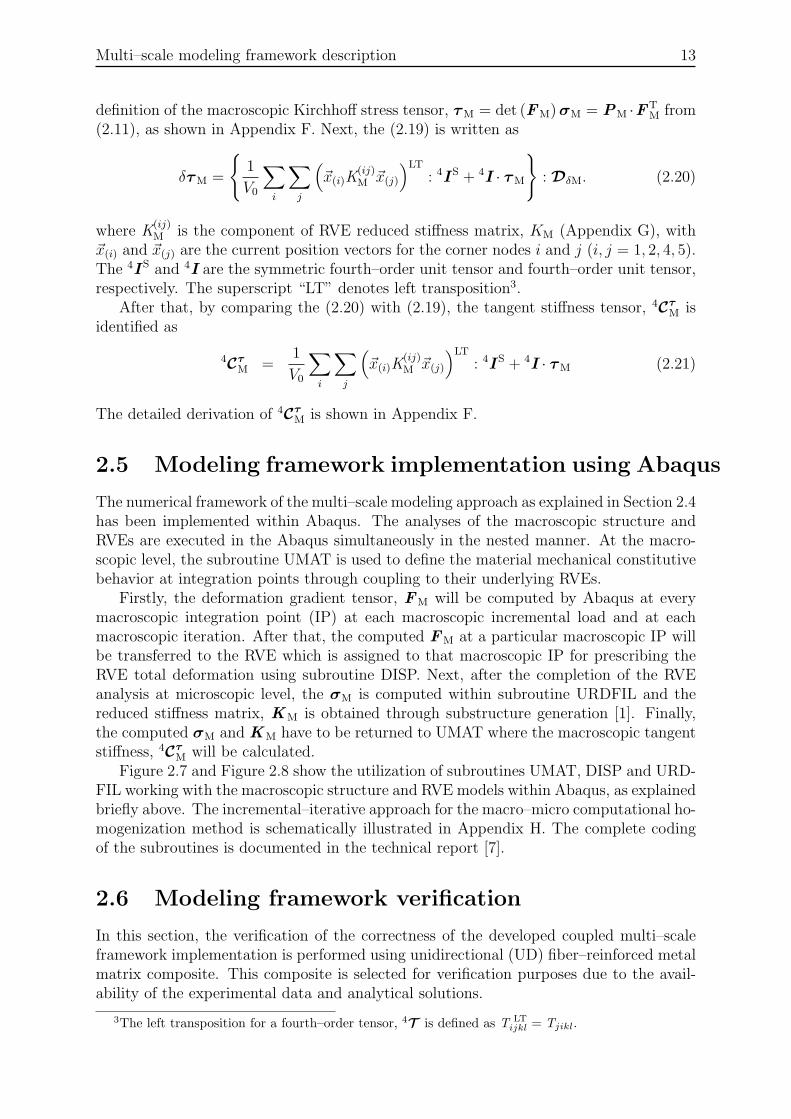
The numerical framework of the multi–scale modeling approach as explained in Section 2.4has been implemented within Abaqus. The analyses of the macroscopic structure andRVEs are executed in the Abaqus simultaneously in the nested manner. At the macro-scopic level, the subroutine UMAT is used to define the material mechanical constitutivebehavior at integration points through coupling to their underlying RVEs.
Firstly, the deformation gradient tensor, FM will be computed by Abaqus at everymacroscopic integration point (IP) at each macroscopic incremental load and at eachmacroscopic iteration. After that, the computed FM at a particular macroscopic IP willbe transferred to the RVE which is assigned to that macroscopic IP for prescribing theRVE total deformation using subroutine DISP. Next, after the completion of the RVEanalysis at microscopic level, the σM is computed within subroutine URDFIL and thereduced stiffness matrix, KM is obtained through substructure generation [1]. Finally,the computed σM and KM have to be returned to UMAT where the macroscopic tangentstiffness, 4C
τ
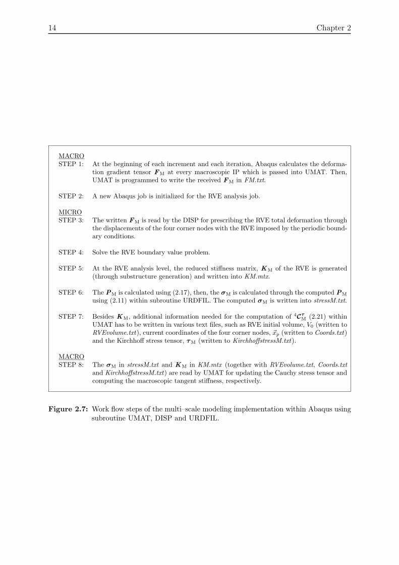
M will be calculated.Figure 2.7 and Figure 2.8 show the utilization of subroutines UMAT, DISP and URD-
FIL working with the macroscopic structure and RVE models within Abaqus, as explainedbriefly above. The incremental–iterative approach for the macro–micro computational ho-mogenization method is schematically illustrated in Appendix H. The complete codingof the subroutines is documented in the technical report [7].
2.6 Modeling framework verification
In this section, the verification of the correctness of the developed coupled multi–scaleframework implementation is performed using unidirectional (UD) fiber–reinforced metalmatrix composite. This composite is selected for verification purposes due to the avail-ability of the experimental data and analytical solutions.
3The left transposition for a fourth–order tensor, 4T is defined as T LT
ijkl = Tjikl.
14 Chapter 2
MACROSTEP 1: At the beginning of each increment and each iteration, Abaqus calculates the deforma-
tion gradient tensor FM at every macroscopic IP which is passed into UMAT. Then,UMAT is programmed to write the received FM in FM.txt.
STEP 2: A new Abaqus job is initialized for the RVE analysis job.
MICROSTEP 3: The written FM is read by the DISP for prescribing the RVE total deformation through
the displacements of the four corner nodes with the RVE imposed by the periodic bound-ary conditions.
STEP 4: Solve the RVE boundary value problem.
STEP 5: At the RVE analysis level, the reduced stiffness matrix, KM of the RVE is generated(through substructure generation) and written into KM.mtx.
STEP 6: The PM is calculated using (2.17), then, the σM is calculated through the computed PM
using (2.11) within subroutine URDFIL. The computed σM is written into stressM.txt.
STEP 7: Besides KM, additional information needed for the computation of 4Cτ
M(2.21) within
UMAT has to be written in various text files, such as RVE initial volume, V0 (written toRVEvolume.txt), current coordinates of the four corner nodes, ~xp (written to Coords.txt)and the Kirchhoff stress tensor, τM (written to KirchhoffstressM.txt).
MACROSTEP 8: The σM in stressM.txt and KM in KM.mtx (together with RVEvolume.txt, Coords.txt
and KirchhoffstressM.txt) are read by UMAT for updating the Cauchy stress tensor andcomputing the macroscopic tangent stiffness, respectively.
Figure 2.7: Work flow steps of the multi–scale modeling implementation within Abaqus usingsubroutine UMAT, DISP and URDFIL.
Multi–scale modeling framework description 15
Abaqus
Macro-structureAbaqus
Micro-structuremacro_structure.inp
UMAT.for
micro_structure.inp
user_subroutine.for
FM.txt
*Heading
...
*Boundary, user
*Substructure
Generate
*Substructure matrix
output, stiffness=YES
KM.mtx
subroutine DISP
subroutine URDFIL
*Heading
...
*user material
subroutine UMAT
execute Abaqus micro-
structure analysis job
STRESS(NTENS)
DFGRD1(I,J)
DDSDDE(NTENS,
NTENS)
CauchystressM.txt
KirchhoffstressM.txt
RVEvolume.txt
Coords.txt
Figure 2.8: Schematic view of the multi–scale numerical framework implemented withinAbaqus.
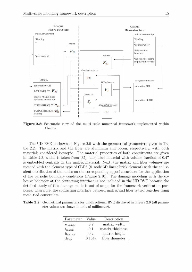
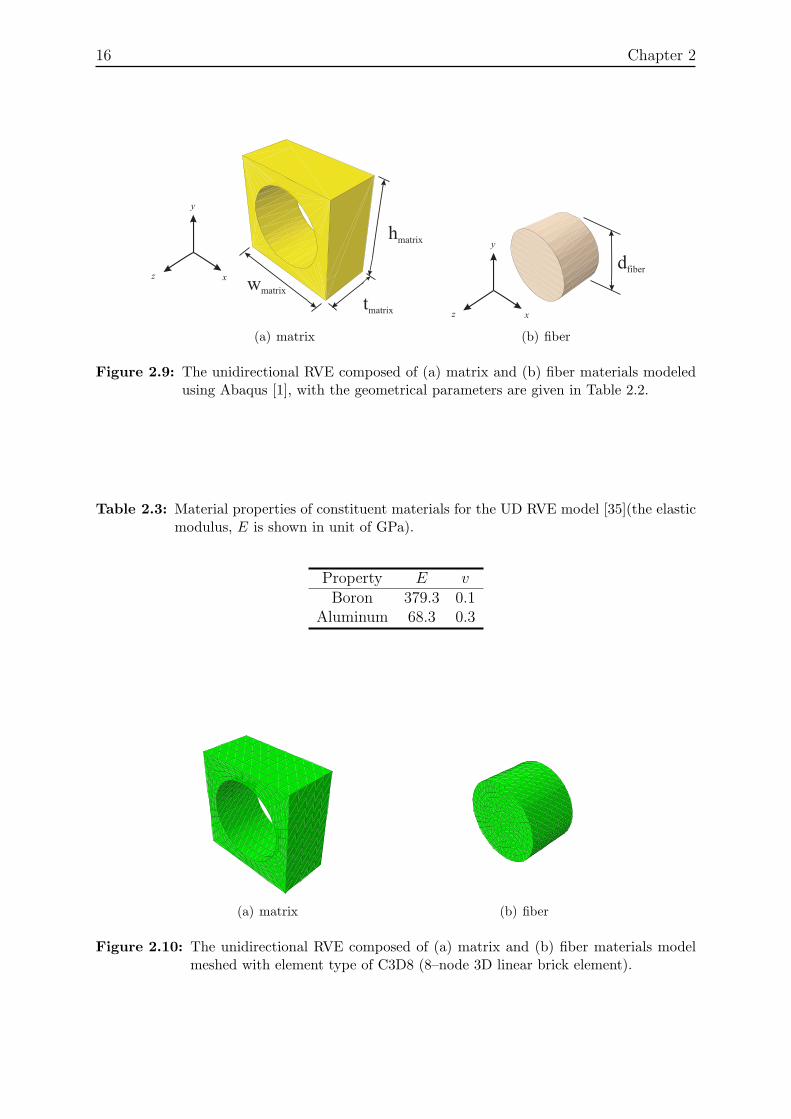
The UD RVE is shown in Figure 2.9 with the geometrical parameters given in Ta-ble 2.2. The matrix and the fiber are aluminum and boron, respectively, with bothmaterials considered isotropic. The material properties of both constituents are givenin Table 2.3, which is taken from [35]. The fiber material with volume fraction of 0.47is embedded centrally in the matrix material. Next, the matrix and fiber volumes aremeshed with the element type of C3D8 (8–node 3D linear brick element) with the equiv-alent distribution of the nodes on the corresponding opposite surfaces for the applicationof the periodic boundary conditions (Figure 2.10). The damage modeling with the co-hesive behavior at the contacting interface is not included in the UD RVE because thedetailed study of this damage mode is out of scope for the framework verification pur-poses. Therefore, the contacting interface between matrix and fiber is tied together usingmesh tied constraints.
Table 2.2: Geometrical parameters for unidirectional RVE displayed in Figure 2.9 (all param-eter values are shown in unit of millimeter).
Parameter Value Description
wmatrix 0.2 matrix widthtmatrix 0.1 matrix thicknesshmatrix 0.2 matrix heightdfiber 0.1547 fiber diameter
16 Chapter 2
y
xz
hmatrix
tmatrix
wmatrix
(a) matrix
y
xz
dfiber
(b) fiber
Figure 2.9: The unidirectional RVE composed of (a) matrix and (b) fiber materials modeledusing Abaqus [1], with the geometrical parameters are given in Table 2.2.
Table 2.3: Material properties of constituent materials for the UD RVE model [35](the elasticmodulus, E is shown in unit of GPa).
Property E vBoron 379.3 0.1
Aluminum 68.3 0.3
(a) matrix (b) fiber
Figure 2.10: The unidirectional RVE composed of (a) matrix and (b) fiber materials modelmeshed with element type of C3D8 (8–node 3D linear brick element).
Multi–scale modeling framework description 17
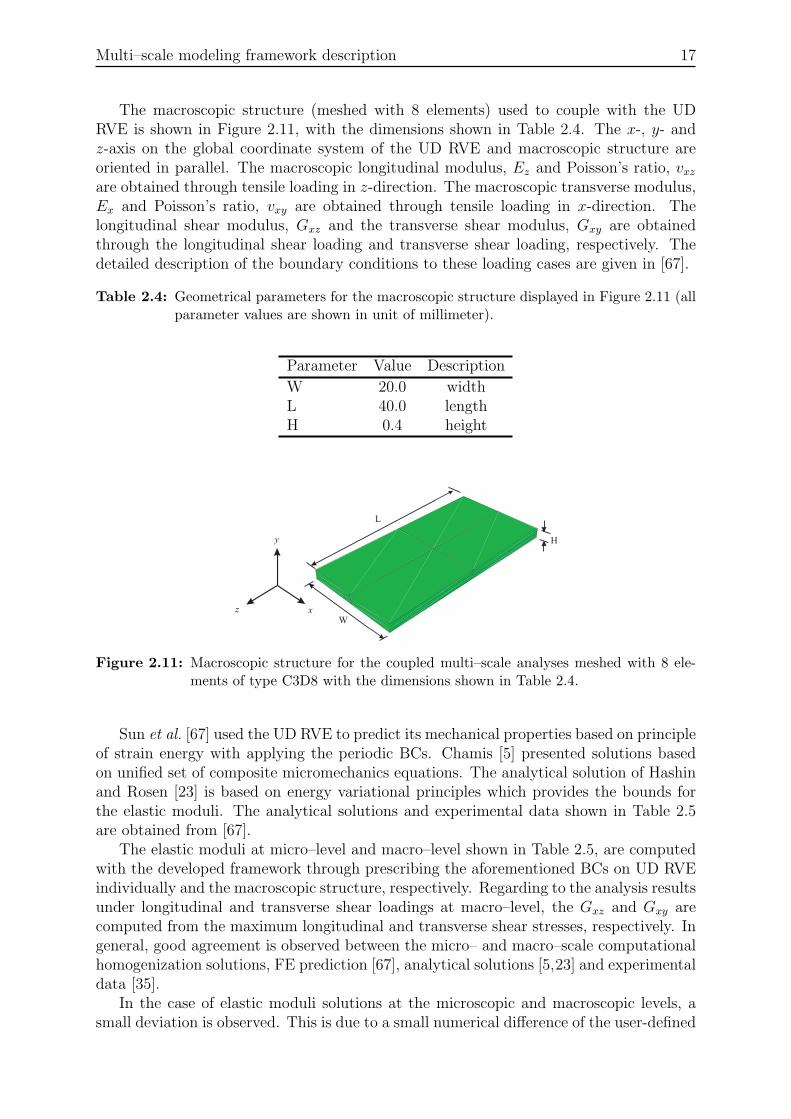
The macroscopic structure (meshed with 8 elements) used to couple with the UDRVE is shown in Figure 2.11, with the dimensions shown in Table 2.4. The x-, y- andz-axis on the global coordinate system of the UD RVE and macroscopic structure areoriented in parallel. The macroscopic longitudinal modulus, Ez and Poisson’s ratio, vxzare obtained through tensile loading in z-direction. The macroscopic transverse modulus,Ex and Poisson’s ratio, vxy are obtained through tensile loading in x-direction. Thelongitudinal shear modulus, Gxz and the transverse shear modulus, Gxy are obtainedthrough the longitudinal shear loading and transverse shear loading, respectively. Thedetailed description of the boundary conditions to these loading cases are given in [67].
Table 2.4: Geometrical parameters for the macroscopic structure displayed in Figure 2.11 (allparameter values are shown in unit of millimeter).
Parameter Value Description
W 20.0 widthL 40.0 lengthH 0.4 height
X
Y
Z
y
xz
W
L
H
Figure 2.11: Macroscopic structure for the coupled multi–scale analyses meshed with 8 ele-ments of type C3D8 with the dimensions shown in Table 2.4.
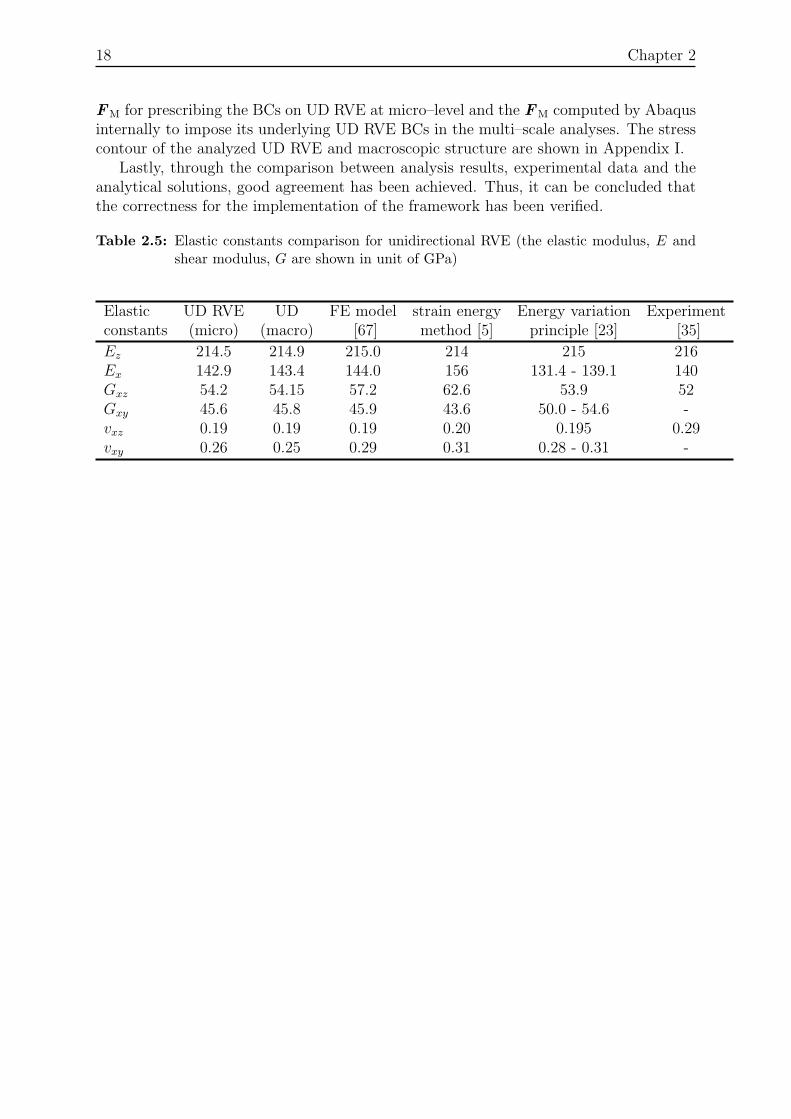
Sun et al. [67] used the UD RVE to predict its mechanical properties based on principleof strain energy with applying the periodic BCs. Chamis [5] presented solutions basedon unified set of composite micromechanics equations. The analytical solution of Hashinand Rosen [23] is based on energy variational principles which provides the bounds forthe elastic moduli. The analytical solutions and experimental data shown in Table 2.5are obtained from [67].
The elastic moduli at micro–level and macro–level shown in Table 2.5, are computedwith the developed framework through prescribing the aforementioned BCs on UD RVEindividually and the macroscopic structure, respectively. Regarding to the analysis resultsunder longitudinal and transverse shear loadings at macro–level, the Gxz and Gxy arecomputed from the maximum longitudinal and transverse shear stresses, respectively. Ingeneral, good agreement is observed between the micro– and macro–scale computationalhomogenization solutions, FE prediction [67], analytical solutions [5,23] and experimentaldata [35].
In the case of elastic moduli solutions at the microscopic and macroscopic levels, asmall deviation is observed. This is due to a small numerical difference of the user-defined
18 Chapter 2
FM for prescribing the BCs on UD RVE at micro–level and the FM computed by Abaqusinternally to impose its underlying UD RVE BCs in the multi–scale analyses. The stresscontour of the analyzed UD RVE and macroscopic structure are shown in Appendix I.
Lastly, through the comparison between analysis results, experimental data and theanalytical solutions, good agreement has been achieved. Thus, it can be concluded thatthe correctness for the implementation of the framework has been verified.
Table 2.5: Elastic constants comparison for unidirectional RVE (the elastic modulus, E andshear modulus, G are shown in unit of GPa)
Elastic UD RVE UD FE model strain energy Energy variation Experimentconstants (micro) (macro) [67] method [5] principle [23] [35]
Ez 214.5 214.9 215.0 214 215 216Ex 142.9 143.4 144.0 156 131.4 - 139.1 140Gxz 54.2 54.15 57.2 62.6 53.9 52Gxy 45.6 45.8 45.9 43.6 50.0 - 54.6 -vxz 0.19 0.19 0.19 0.20 0.195 0.29vxy 0.26 0.25 0.29 0.31 0.28 - 0.31 -
Chapter 3
Micro–structural modeling
3.1 Textile and non–crimp composite models
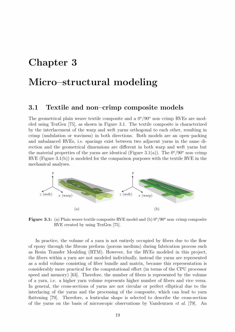
The geometrical plain weave textile composite and a 0o/90o non–crimp RVEs are mod-eled using TexGen [75], as shown in Figure 3.1. The textile composite is characterizedby the interlacement of the warp and weft yarns orthogonal to each other, resulting incrimp (undulation or waviness) in both directions. Both models are an open–packingand unbalanced RVEs, i.e. spacings exist between two adjacent yarns in the same di-rection and the geometrical dimensions are different in both warp and weft yarns butthe material properties of the yarns are identical (Figure 3.1(a)). The 0o/90o non–crimpRVE (Figure 3.1(b)) is modeled for the comparison purposes with the textile RVE in themechanical analyses.
x (warp)
y
z (weft)
(a)
x (warp)
y
z (weft)
(b)
Figure 3.1: (a) Plain weave textile composite RVE model and (b) 0o/90o non–crimp compositeRVE created by using TexGen [75].
In practice, the volume of a yarn is not entirely occupied by fibers due to the flowof epoxy through the fibrous preform (porous medium) during fabrication process suchas Resin Transfer Moulding (RTM). However, for the RVEs modeled in this project,the fibers within a yarn are not modeled individually, instead the yarns are representedas a solid volume consisting of fiber bundle and matrix, because this representation isconsiderably more practical for the computational effort (in terms of the CPU processorspeed and memory) [63]. Therefore, the number of fibers is represented by the volumeof a yarn, i.e. a higher yarn volume represents higher number of fibers and vice versa.In general, the cross-sections of yarns are not circular or perfect elliptical due to theinterlacing of the yarns and the processing of the composite, which can lead to yarnflattening [79]. Therefore, a lenticular shape is selected to describe the cross-sectionof the yarns on the basis of microscopic observations by Vandeurzen et al. [79]. An
19
20 Chapter 3
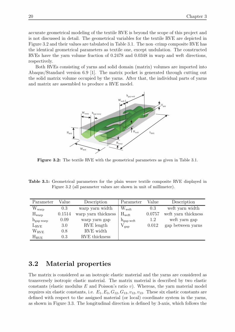
accurate geometrical modeling of the textile RVE is beyond the scope of this project andis not discussed in detail. The geometrical variables for the textile RVE are depicted inFigure 3.2 and their values are tabulated in Table 3.1. The non–crimp composite RVE hasthe identical geometrical parameters as textile one, except undulation. The constructedRVEs have the yarn volume fraction of 0.2478 and 0.0348 in warp and weft directions,respectively.
Both RVEs consisting of yarns and solid domain (matrix) volumes are imported intoAbaqus/Standard version 6.9 [1]. The matrix pocket is generated through cutting outthe solid matrix volume occupied by the yarns. After that, the individual parts of yarnsand matrix are assembled to produce a RVE model.
WRVE
LRVEHRVE
hgap warpWwarp
Hwarp
Vgap
Wweft
hgap weft
Hweft
Figure 3.2: The textile RVE with the geometrical parameters as given in Table 3.1.
Table 3.1: Geometrical parameters for the plain weave textile composite RVE displayed inFigure 3.2 (all parameter values are shown in unit of millimeter).
Parameter Value Description Parameter Value Description
Wwarp 0.3 warp yarn width Wweft 0.3 weft yarn widthHwarp 0.1514 warp yarn thickness Hweft 0.0757 weft yarn thicknesshgap warp 0.09 warp yarn gap hgap weft 1.2 weft yarn gapLRVE 3.0 RVE length Vgap 0.012 gap between yarnsWRVE 0.8 RVE widthHRVE 0.3 RVE thickness
3.2 Material properties
The matrix is considered as an isotropic elastic material and the yarns are considered astransversely isotropic elastic material. The matrix material is described by two elasticconstants (elastic modulus E and Poisson’s ratio v). Whereas, the yarn material modelrequires six elastic constants, i.e. E1, E3, G12, G13, v12, v13. These six elastic constants aredefined with respect to the assigned material (or local) coordinate system in the yarns,as shown in Figure 3.3. The longitudinal direction is defined by 3-axis, which follows the
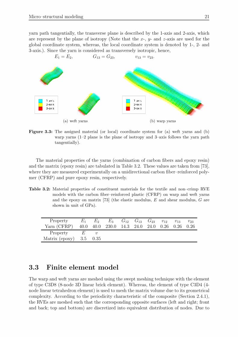
Micro–structural modeling 21
yarn path tangentially, the transverse plane is described by the 1-axis and 2-axis, whichare represent by the plane of isotropy (Note that the x-, y- and z-axis are used for theglobal coordinate system, whereas, the local coordinate system is denoted by 1-, 2- and3-axis.). Since the yarn is considered as transversely isotropic, hence,
E1 = E2, G13 = G23, v13 = v23.
(a) weft yarns (b) warp yarns
Figure 3.3: The assigned material (or local) coordinate system for (a) weft yarns and (b)warp yarns (1–2 plane is the plane of isotropy and 3–axis follows the yarn pathtangentially).
The material properties of the yarns (combination of carbon fibers and epoxy resin)and the matrix (epoxy resin) are tabulated in Table 3.2. These values are taken from [73],where they are measured experimentally on a unidirectional carbon fiber–reinforced poly-mer (CFRP) and pure epoxy resin, respectively.
Table 3.2: Material properties of constituent materials for the textile and non–crimp RVEmodels with the carbon fiber–reinforced plastic (CFRP) on warp and weft yarnsand the epoxy on matrix [73] (the elastic modulus, E and shear modulus, G areshown in unit of GPa).
Property E1 E2 E3 G12 G13 G23 v12 v13 v23Yarn (CFRP) 40.0 40.0 230.0 14.3 24.0 24.0 0.26 0.26 0.26
Property E vMatrix (epoxy) 3.5 0.35
3.3 Finite element model
The warp and weft yarns are meshed using the swept meshing technique with the elementof type C3D8 (8-node 3D linear brick element). Whereas, the element of type C3D4 (4-node linear tetrahedron element) is used to mesh the matrix volume due to its geometricalcomplexity. According to the periodicity characteristic of the composite (Section 2.4.1),the RVEs are meshed such that the corresponding opposite surfaces (left and right; frontand back; top and bottom) are discretized into equivalent distribution of nodes. Due to
22 Chapter 3
the incompatible element types of both volumes, the contacting interfaces between theyarns and matrix are tied together with the mesh tie constraint.
In practice, the interfacial debonding between the fiber and matrix can occur duringthe fabrication process (due to the mismatch of their thermal expansion coefficients) [81].However, the interfacial debonding between the fiber and matrix is not considered in thisproject because the micro–structure constituted of the fibers and the matrix within theyarn is not modeled, as explained earlier. Therefore, the mesh tie constraint between theyarns and matrix interfaces is used to simulate the perfect bonding between both volumes.Moreover, the perfect bonding is justified to reduce the computational cost and time, sincethe interface formulation can increase the cost and time dramatically [14, 92, 95].
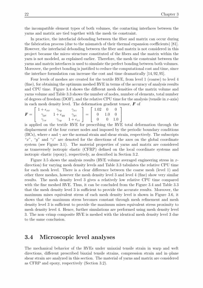
Four levels of meshes are created for the textile RVE, from level 1 (coarse) to level 4(fine), for obtaining the optimum meshed RVE in terms of the accuracy of analysis resultsand CPU time. Figure 3.4 shows the different mesh densities of the matrix volume andyarns volume and Table 3.3 shows the number of nodes, number of elements, total numberof degrees of freedom (DOF), and the relative CPU time for the analysis (tensile in x-axis)in each mesh density level. The deformation gradient tensor, F of
F =
1 + εxx γxy γxzγyx 1 + εyy γyzγzx γzy 1 + εzz
=
1.02 0 00 1.0 00 0 1.0
is applied on the textile RVE for prescribing the RVE total deformation through thedisplacement of the four corner nodes and imposed by the periodic boundary conditions(BCs), where ε and γ are the normal strain and shear strain, respectively. The subscripts“x”, “y” and “z” are denoted for the directions of the axes on the global coordinatesystem (see Figure 3.1). The material properties of yarns and matrix are consideredas transversely isotropic elastic (CFRP) defined on the local coordinate systems andisotropic elastic (epoxy), respectively, as described in Section 3.2.
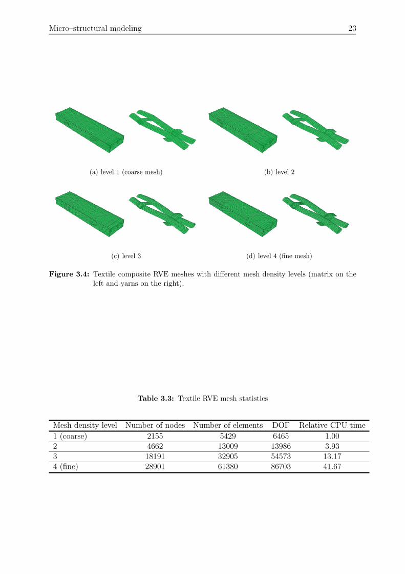
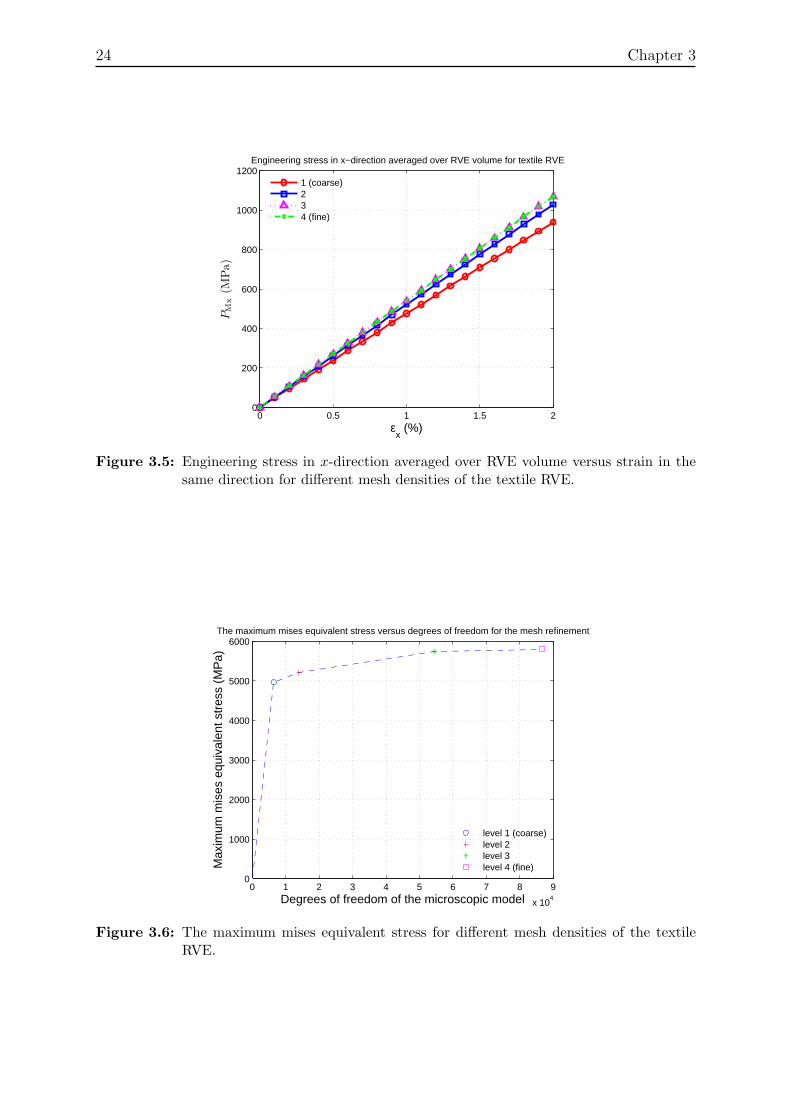
Figure 3.5 shows the analysis results (RVE volume averaged engineering stress in x-direction) for varying mesh density levels and Table 3.3 tabulates the relative CPU timefor each mesh level. There is a clear difference between the coarse mesh (level 1) andother three meshes, however the mesh density level 3 and level 4 (fine) show very similarresults. The mesh density level 3 gives a relatively low relative CPU time comparedwith the fine meshed RVE. Thus, it can be concluded from the Figure 3.4 and Table 3.3that the mesh density level 3 is sufficient to provide the accurate results. Moreover, themaximum mises equivalent stress of each mesh density level is shown in Figure 3.6, itshows that the maximum stress becomes constant through mesh refinement and meshdensity level 3 is sufficient to provide the maximum mises equivalent stress proximity tomesh density level 4. Hence, further simulations are performed using mesh density level3. The non–crimp composite RVE is meshed with the identical mesh density level 3 dueto the same conclusion.
3.4 Microscopic level analyses
The mechanical behavior of the RVEs under uniaxial tensile strain in warp and weftdirections, different prescribed biaxial tensile strains, compression strain and in–planeshear strain are analyzed in this section. The material of yarns and matrix are consideredas CFRP and epoxy, respectively (Section 3.2).
Micro–structural modeling 23
(a) level 1 (coarse mesh) (b) level 2
(c) level 3 (d) level 4 (fine mesh)
Figure 3.4: Textile composite RVE meshes with different mesh density levels (matrix on theleft and yarns on the right).
Table 3.3: Textile RVE mesh statistics
Mesh density level Number of nodes Number of elements DOF Relative CPU time
1 (coarse) 2155 5429 6465 1.002 4662 13009 13986 3.933 18191 32905 54573 13.174 (fine) 28901 61380 86703 41.67
24 Chapter 3
0 0.5 1 1.5 20
200
400
600
800
1000
1200
εx (%)
PM
x(M
Pa)
Engineering stress in x−direction averaged over RVE volume for textile RVE
1 (coarse)234 (fine)
Figure 3.5: Engineering stress in x-direction averaged over RVE volume versus strain in thesame direction for different mesh densities of the textile RVE.
0 1 2 3 4 5 6 7 8 9
x 104
0
1000
2000
3000
4000
5000
6000
Degrees of freedom of the microscopic model
Max
imum
mis
es e
quiv
alen
t str
ess
(MP
a)
The maximum mises equivalent stress versus degrees of freedom for the mesh refinement
level 1 (coarse)level 2level 3level 4 (fine)
Figure 3.6: The maximum mises equivalent stress for different mesh densities of the textileRVE.
Micro–structural modeling 25
3.4.1 Tension test
The characteristic of crimp of the yarns has a significant influence on the mechanicalbehavior of a composite structure. In the case of uniaxial tensile strain on a textile RVE,yarns under tensile strain tend to straighten, whereas, the crimp of yarns in transversedirection tend to increase. This phenomenon is called crimp interchange and it occurs inthe case of biaxial tensile strain as well, i.e. the yarns in one direction has an influence onthe behavior of the yarns in transverse direction. The nature of crimp interchange can beinfluenced by the geometrical properties of the yarns and it has a significant influence onthe strength of a composite structure [59]. The mechanical response of the RVEs underuniaxial tension tests is studied first, followed by the biaxial tension tests.
3.4.1.1 Uniaxial tension
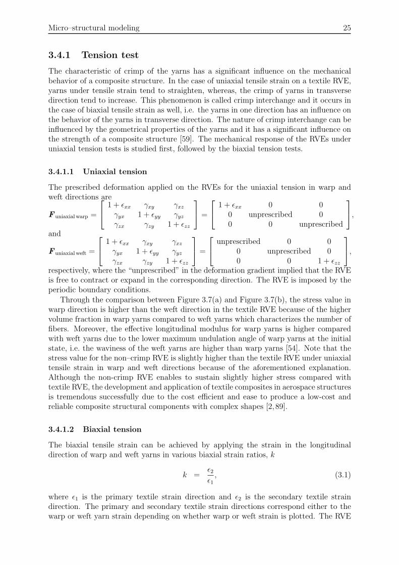
The prescribed deformation applied on the RVEs for the uniaxial tension in warp andweft directions are
F uniaxial warp =
1 + εxx γxy γxzγyx 1 + εyy γyzγzx γzy 1 + εzz
=
1 + εxx 0 00 unprescribed 00 0 unprescribed
,
and
F uniaxial weft =
1 + εxx γxy γxzγyx 1 + εyy γyzγzx γzy 1 + εzz
=
unprescribed 0 00 unprescribed 00 0 1 + εzz
,
respectively, where the “unprescribed” in the deformation gradient implied that the RVEis free to contract or expand in the corresponding direction. The RVE is imposed by theperiodic boundary conditions.
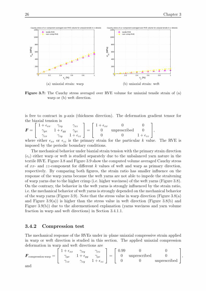
Through the comparison between Figure 3.7(a) and Figure 3.7(b), the stress value inwarp direction is higher than the weft direction in the textile RVE because of the highervolume fraction in warp yarns compared to weft yarns which characterizes the number offibers. Moreover, the effective longitudinal modulus for warp yarns is higher comparedwith weft yarns due to the lower maximum undulation angle of warp yarns at the initialstate, i.e. the waviness of the weft yarns are higher than warp yarns [54]. Note that thestress value for the non–crimp RVE is slightly higher than the textile RVE under uniaxialtensile strain in warp and weft directions because of the aforementioned explanation.Although the non-crimp RVE enables to sustain slightly higher stress compared withtextile RVE, the development and application of textile composites in aerospace structuresis tremendous successfully due to the cost efficient and ease to produce a low-cost andreliable composite structural components with complex shapes [2, 89].
3.4.1.2 Biaxial tension
The biaxial tensile strain can be achieved by applying the strain in the longitudinaldirection of warp and weft yarns in various biaxial strain ratios, k
k =ε2ε1, (3.1)
where ε1 is the primary textile strain direction and ε2 is the secondary textile straindirection. The primary and secondary textile strain directions correspond either to thewarp or weft yarn strain depending on whether warp or weft strain is plotted. The RVE
26 Chapter 3
0 0.2 0.4 0.6 0.8 10
200
400
600
800
1000
1200
εx (%)
σ xx (
MP
a)Cauchy stress of xx−component averaged over RVE volume for uniaxial tensile in x−direction
textile RVEnon−crimp RVE
(a) uniaxial strain: warp
0 0.2 0.4 0.6 0.8 10
200
400
600
800
1000
1200
εz (%)
σ zz (
MP
a)
Cauchy stress of zz−component averaged over RVE volume for uniaxial tensile in z−direction
textile RVEnon−crimp RVE
(b) uniaxial strain: weft
Figure 3.7: The Cauchy stress averaged over RVE volume for uniaxial tensile strain of (a)warp or (b) weft direction.
is free to contract in y-axis (thickness direction). The deformation gradient tensor forthe biaxial tension is
F =
1 + εxx γxy γxzγyx 1 + εyy γyzγzx γzy 1 + εzz
=
1 + εxx 0 00 unprescribed 00 0 1 + εzz
,
where either εxx or εzz is the primary strain for the particular k value. The RVE isimposed by the periodic boundary conditions.
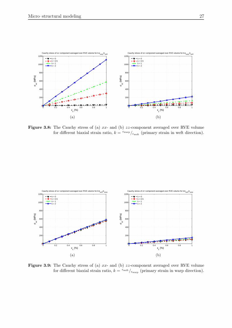
The mechanical behavior under biaxial strain tension with the primary strain direction(ε1) either warp or weft is studied separately due to the unbalanced yarn nature in thetextile RVE. Figure 3.8 and Figure 3.9 show the computed volume averaged Cauchy stressof xx- and zz-component for different k values of weft and warp as primary direction,respectively. By comparing both figures, the strain ratio has smaller influence on theresponse of the warp yarns because the weft yarns are not able to impede the straiteningof warp yarns due to the higher crimp (i.e. higher waviness) of the weft yarns (Figure 3.8).On the contrary, the behavior in the weft yarns is strongly influenced by the strain ratio,i.e. the mechanical behavior of weft yarns is strongly depended on the mechanical behaviorof the warp yarns (Figure 3.9). Note that the stress value in warp direction (Figure 3.8(a)and Figure 3.9(a)) is higher than the stress value in weft direction (Figure 3.8(b) andFigure 3.9(b)) due to the aforementioned explanation (yarns waviness and yarn volumefraction in warp and weft directions) in Section 3.4.1.1.
3.4.2 Compression test
The mechanical response of the RVEs under in–plane uniaxial compressive strain appliedin warp or weft direction is studied in this section. The applied uniaxial compressiondeformation in warp and weft directions are
F compressionwarp =
1 + εxx γxy γxzγyx 1 + εyy γyzγzx γzy 1 + εzz
=
0.99 0 00 unprescribed 00 0 unprescribed
,
and
Micro–structural modeling 27
0 0.2 0.4 0.6 0.8 10
200
400
600
800
1000
1200
εx (%)
σ xx (
MP
a)
Cauchy stress of xx−component averaged over RVE volume for k=εwarp
/εweft
k = 0k = 0.5k = 1k = 2
(a)
0 0.2 0.4 0.6 0.8 10
200
400
600
800
1000
1200
εz (%)
σ zz (
MP
a)
Cauchy stress of zz−component averaged over RVE volume for k=εwarp
/εweft
k = 0k = 0.5k = 1k = 2
(b)
Figure 3.8: The Cauchy stress of (a) xx- and (b) zz-component averaged over RVE volumefor different biaxial strain ratio, k = εwarp/εweft
(primary strain in weft direction).
0 0.2 0.4 0.6 0.8 10
200
400
600
800
1000
1200
εx (%)
σ xx (
MP
a)
Cauchy stress of xx−component averaged over RVE volume for k=εweft
/εwarp
k = 0k = 0.5k = 1k = 2
(a)
0 0.2 0.4 0.6 0.8 10
200
400
600
800
1000
1200
εz (%)
σ zz (
MP
a)
Cauchy stress of zz−component averaged over RVE volume for k=εweft
/εwarp
k = 0k = 0.5k = 1k = 2
(b)
Figure 3.9: The Cauchy stress of (a) xx- and (b) zz-component averaged over RVE volumefor different biaxial strain ratio, k = εweft/εwarp (primary strain in warp direction).
28 Chapter 3
F compressionweft =
1 + εxx γxy γxzγyx 1 + εyy γyzγzx γzy 1 + εzz
=
unprescribed 0 00 unprescribed 00 0 0.99
,
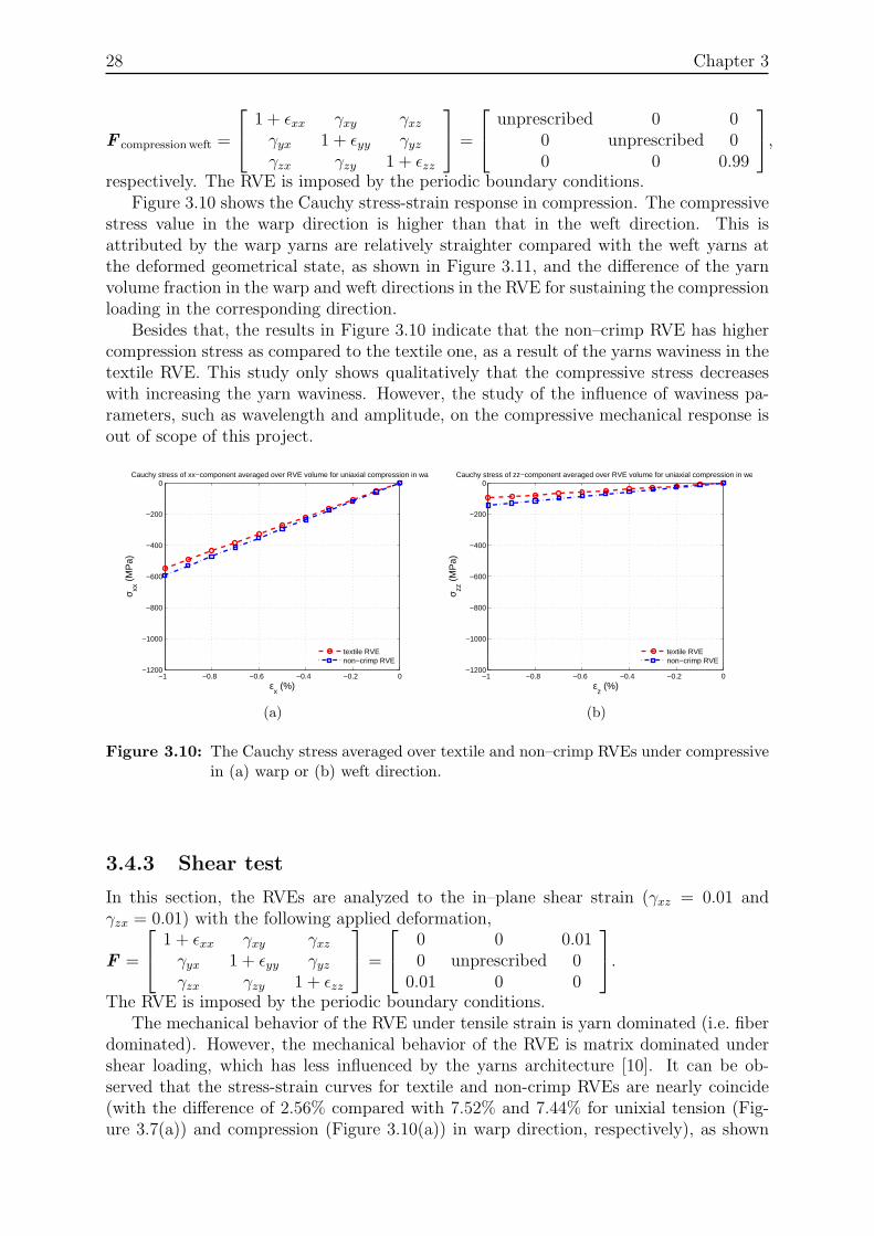
respectively. The RVE is imposed by the periodic boundary conditions.Figure 3.10 shows the Cauchy stress-strain response in compression. The compressive
stress value in the warp direction is higher than that in the weft direction. This isattributed by the warp yarns are relatively straighter compared with the weft yarns atthe deformed geometrical state, as shown in Figure 3.11, and the difference of the yarnvolume fraction in the warp and weft directions in the RVE for sustaining the compressionloading in the corresponding direction.
Besides that, the results in Figure 3.10 indicate that the non–crimp RVE has highercompression stress as compared to the textile one, as a result of the yarns waviness in thetextile RVE. This study only shows qualitatively that the compressive stress decreaseswith increasing the yarn waviness. However, the study of the influence of waviness pa-rameters, such as wavelength and amplitude, on the compressive mechanical response isout of scope of this project.
−1 −0.8 −0.6 −0.4 −0.2 0−1200
−1000
−800
−600
−400
−200
0
εx (%)
σ xx (
MP
a)
Cauchy stress of xx−component averaged over RVE volume for uniaxial compression in warp
textile RVEnon−crimp RVE
(a)
−1 −0.8 −0.6 −0.4 −0.2 0−1200
−1000
−800
−600
−400
−200
0
εz (%)
σ zz (
MP
a)
Cauchy stress of zz−component averaged over RVE volume for uniaxial compression in weft
textile RVEnon−crimp RVE
(b)
Figure 3.10: The Cauchy stress averaged over textile and non–crimp RVEs under compressivein (a) warp or (b) weft direction.
3.4.3 Shear test
In this section, the RVEs are analyzed to the in–plane shear strain (γxz = 0.01 andγzx = 0.01) with the following applied deformation,
F =
1 + εxx γxy γxzγyx 1 + εyy γyzγzx γzy 1 + εzz
=
0 0 0.010 unprescribed 0
0.01 0 0
.
The RVE is imposed by the periodic boundary conditions.The mechanical behavior of the RVE under tensile strain is yarn dominated (i.e. fiber
dominated). However, the mechanical behavior of the RVE is matrix dominated undershear loading, which has less influenced by the yarns architecture [10]. It can be ob-served that the stress-strain curves for textile and non-crimp RVEs are nearly coincide(with the difference of 2.56% compared with 7.52% and 7.44% for unixial tension (Fig-ure 3.7(a)) and compression (Figure 3.10(a)) in warp direction, respectively), as shown
Micro–structural modeling 29
(a) (b)
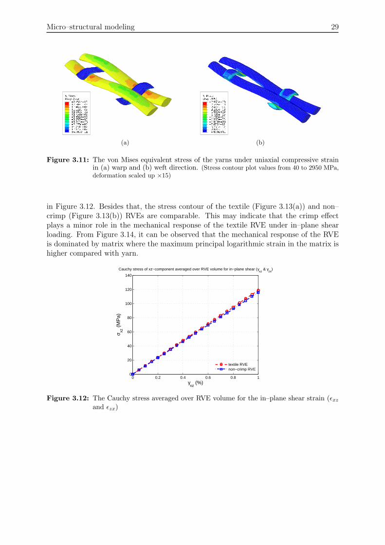
Figure 3.11: The von Mises equivalent stress of the yarns under uniaxial compressive strainin (a) warp and (b) weft direction. (Stress contour plot values from 40 to 2950 MPa,deformation scaled up ×15)
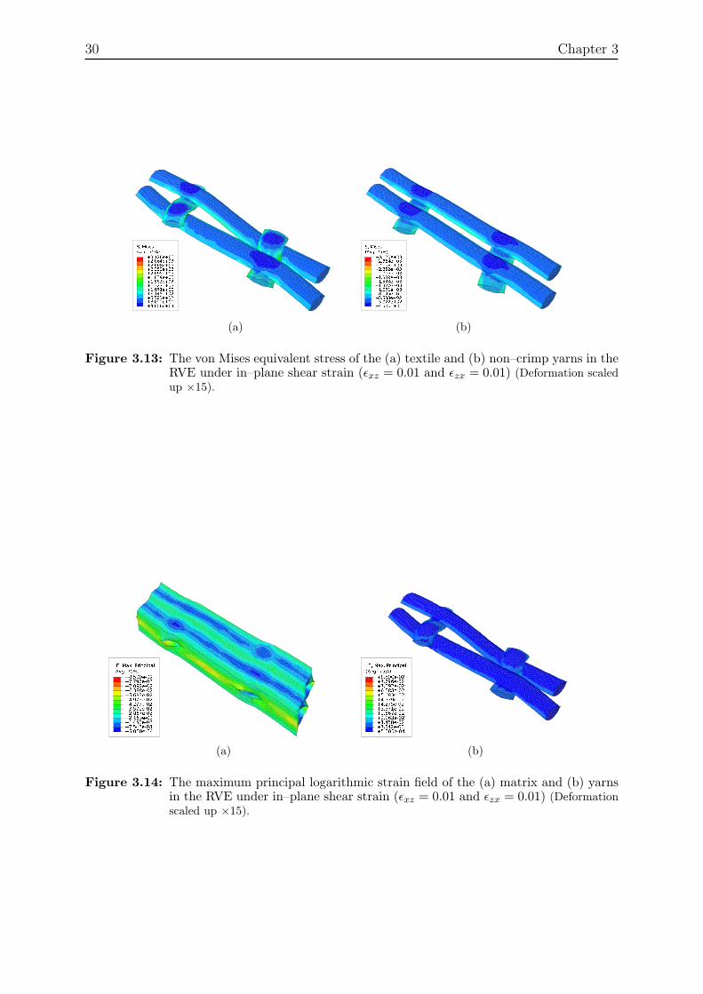
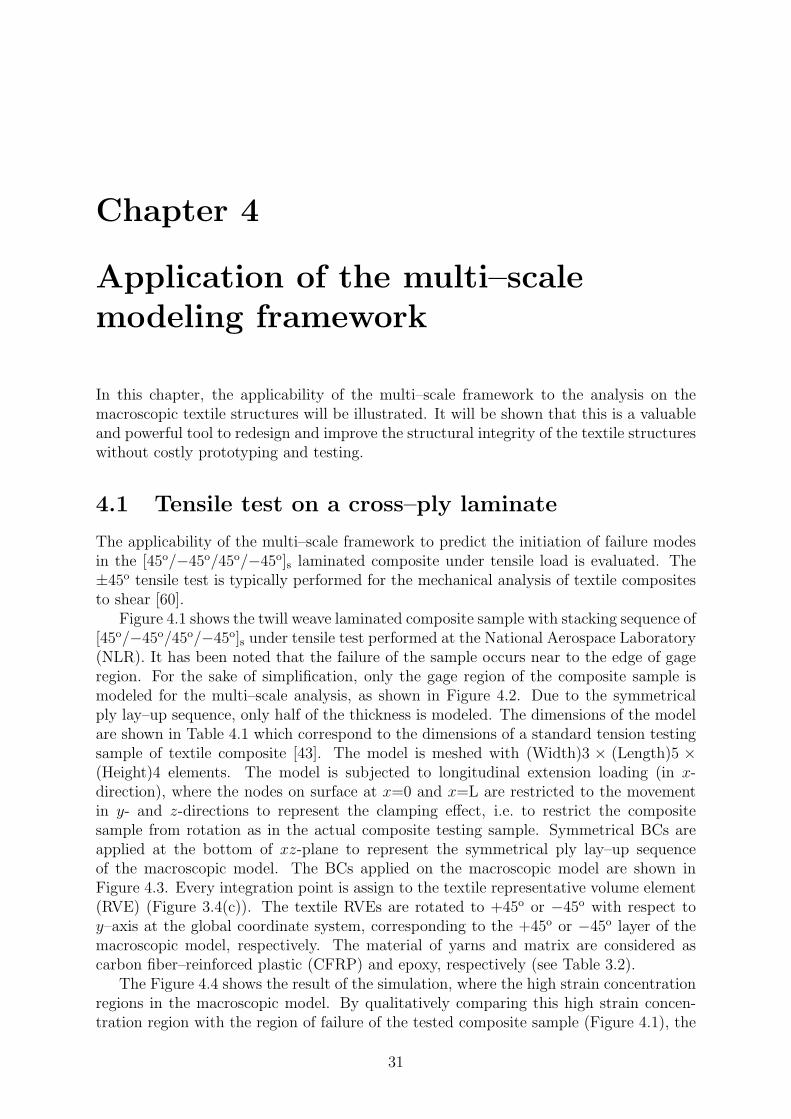
in Figure 3.12. Besides that, the stress contour of the textile (Figure 3.13(a)) and non–crimp (Figure 3.13(b)) RVEs are comparable. This may indicate that the crimp effectplays a minor role in the mechanical response of the textile RVE under in–plane shearloading. From Figure 3.14, it can be observed that the mechanical response of the RVEis dominated by matrix where the maximum principal logarithmic strain in the matrix ishigher compared with yarn.
0 0.2 0.4 0.6 0.8 10
20
40
60
80
100
120
140
γxz
(%)
σ xz (
MP
a)
Cauchy stress of xz−component averaged over RVE volume for in−plane shear ( γxz
& γzx
)
textile RVEnon−crimp RVE
Figure 3.12: The Cauchy stress averaged over RVE volume for the in–plane shear strain (εxzand εzx)
30 Chapter 3
(a) (b)
Figure 3.13: The von Mises equivalent stress of the (a) textile and (b) non–crimp yarns in theRVE under in–plane shear strain (εxz = 0.01 and εzx = 0.01) (Deformation scaledup ×15).
(a) (b)
Figure 3.14: The maximum principal logarithmic strain field of the (a) matrix and (b) yarnsin the RVE under in–plane shear strain (εxz = 0.01 and εzx = 0.01) (Deformationscaled up ×15).
Chapter 4
Application of the multi–scalemodeling framework
In this chapter, the applicability of the multi–scale framework to the analysis on themacroscopic textile structures will be illustrated. It will be shown that this is a valuableand powerful tool to redesign and improve the structural integrity of the textile structureswithout costly prototyping and testing.
4.1 Tensile test on a cross–ply laminate
The applicability of the multi–scale framework to predict the initiation of failure modesin the [45o/−45o/45o/−45o]s laminated composite under tensile load is evaluated. The±45o tensile test is typically performed for the mechanical analysis of textile compositesto shear [60].
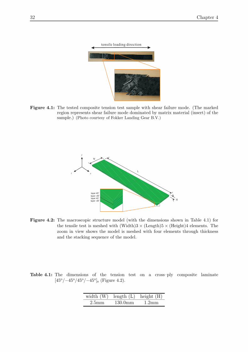
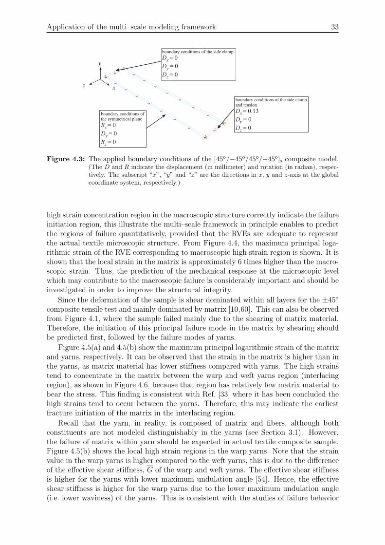
Figure 4.1 shows the twill weave laminated composite sample with stacking sequence of[45o/−45o/45o/−45o]s under tensile test performed at the National Aerospace Laboratory(NLR). It has been noted that the failure of the sample occurs near to the edge of gageregion. For the sake of simplification, only the gage region of the composite sample ismodeled for the multi–scale analysis, as shown in Figure 4.2. Due to the symmetricalply lay–up sequence, only half of the thickness is modeled. The dimensions of the modelare shown in Table 4.1 which correspond to the dimensions of a standard tension testingsample of textile composite [43]. The model is meshed with (Width)3 × (Length)5 ×(Height)4 elements. The model is subjected to longitudinal extension loading (in x-direction), where the nodes on surface at x=0 and x=L are restricted to the movementin y- and z-directions to represent the clamping effect, i.e. to restrict the compositesample from rotation as in the actual composite testing sample. Symmetrical BCs areapplied at the bottom of xz-plane to represent the symmetrical ply lay–up sequenceof the macroscopic model. The BCs applied on the macroscopic model are shown inFigure 4.3. Every integration point is assign to the textile representative volume element(RVE) (Figure 3.4(c)). The textile RVEs are rotated to +45o or −45o with respect toy–axis at the global coordinate system, corresponding to the +45o or −45o layer of themacroscopic model, respectively. The material of yarns and matrix are considered ascarbon fiber–reinforced plastic (CFRP) and epoxy, respectively (see Table 3.2).
The Figure 4.4 shows the result of the simulation, where the high strain concentrationregions in the macroscopic model. By qualitatively comparing this high strain concen-tration region with the region of failure of the tested composite sample (Figure 4.1), the
31
32 Chapter 4
tensile loading direction
Figure 4.1: The tested composite tension test sample with shear failure mode. (The markedregion represents shear failure mode dominated by matrix material (insert) of thesample.) (Photo courtesy of Fokker Landing Gear B.V.)
X
Y
Z
y
xL
W
H
z
layer 45o
layer -45o
layer 45o
layer -45o
Figure 4.2: The macroscopic structure model (with the dimensions shown in Table 4.1) forthe tensile test is meshed with (Width)3 × (Length)5 × (Height)4 elements. Thezoom in view shows the model is meshed with four elements through thicknessand the stacking sequence of the model.
Table 4.1: The dimensions of the tension test on a cross–ply composite laminate[45o/−45o/45o/−45o]s (Figure 4.2).
width (W) length (L) height (H)2.5mm 130.0mm 1.2mm
Application of the multi–scale modeling framework 33
y
xz
boundary conditions of the side clampand tension
Dx = 0.13
D
Dy
z
= 0
= 0
boundary conditions of the side clamp
Dx = 0
D
Dy
z
= 0
= 0
boundary conditions ofthe symmetrical plane
Rx = 0
D
Ry
z
= 0
= 0
Figure 4.3: The applied boundary conditions of the [45o/−45o/45o/−45o]s composite model.(The D and R indicate the displacement (in millimeter) and rotation (in radian), respec-tively. The subscript “x”, “y” and “z” are the directions in x, y and z-axis at the globalcoordinate system, respectively.)
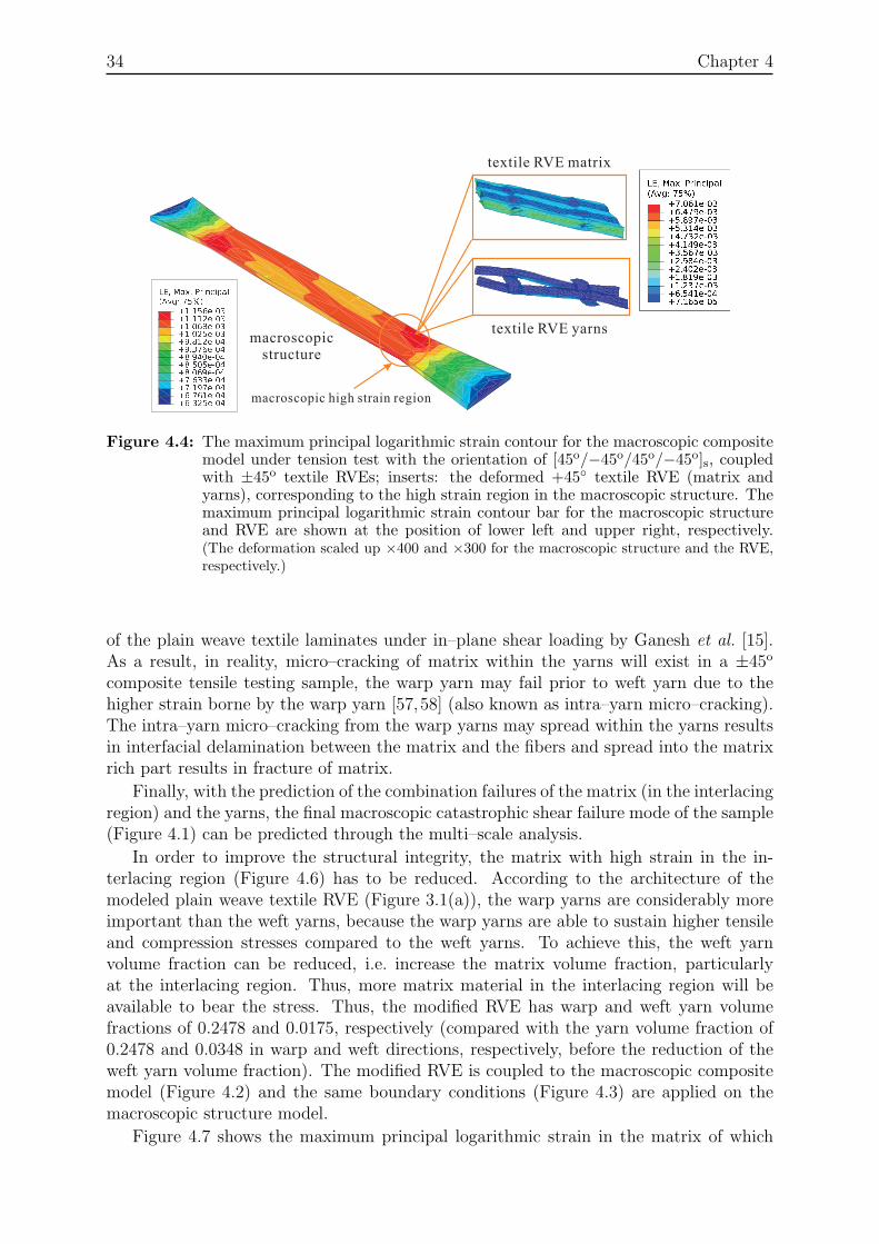
high strain concentration region in the macroscopic structure correctly indicate the failureinitiation region, this illustrate the multi–scale framework in principle enables to predictthe regions of failure quantitatively, provided that the RVEs are adequate to representthe actual textile microscopic structure. From Figure 4.4, the maximum principal loga-rithmic strain of the RVE corresponding to macroscopic high strain region is shown. It isshown that the local strain in the matrix is approximately 6 times higher than the macro-scopic strain. Thus, the prediction of the mechanical response at the microscopic levelwhich may contribute to the macroscopic failure is considerably important and should beinvestigated in order to improve the structural integrity.
Since the deformation of the sample is shear dominated within all layers for the ±45◦
composite tensile test and mainly dominated by matrix [10,60]. This can also be observedfrom Figure 4.1, where the sample failed mainly due to the shearing of matrix material.Therefore, the initiation of this principal failure mode in the matrix by shearing shouldbe predicted first, followed by the failure modes of yarns.
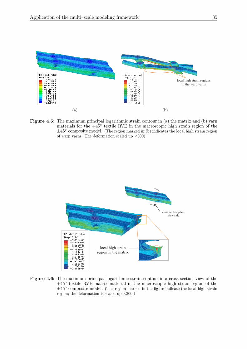
Figure 4.5(a) and 4.5(b) show the maximum principal logarithmic strain of the matrixand yarns, respectively. It can be observed that the strain in the matrix is higher than inthe yarns, as matrix material has lower stiffness compared with yarns. The high strainstend to concentrate in the matrix between the warp and weft yarns region (interlacingregion), as shown in Figure 4.6, because that region has relatively few matrix material tobear the stress. This finding is consistent with Ref. [33] where it has been concluded thehigh strains tend to occur between the yarns. Therefore, this may indicate the earliestfracture initiation of the matrix in the interlacing region.
Recall that the yarn, in reality, is composed of matrix and fibers, although bothconstituents are not modeled distinguishably in the yarns (see Section 3.1). However,the failure of matrix within yarn should be expected in actual textile composite sample.Figure 4.5(b) shows the local high strain regions in the warp yarns. Note that the strainvalue in the warp yarns is higher compared to the weft yarns, this is due to the differenceof the effective shear stiffness, G of the warp and weft yarns. The effective shear stiffnessis higher for the yarns with lower maximum undulation angle [54]. Hence, the effectiveshear stiffness is higher for the warp yarns due to the lower maximum undulation angle(i.e. lower waviness) of the yarns. This is consistent with the studies of failure behavior
34 Chapter 4
macroscopic high strain region
macroscopicstructure
textile RVE matrix
textile RVE yarns
Figure 4.4: The maximum principal logarithmic strain contour for the macroscopic compositemodel under tension test with the orientation of [45o/−45o/45o/−45o]s, coupledwith ±45o textile RVEs; inserts: the deformed +45◦ textile RVE (matrix andyarns), corresponding to the high strain region in the macroscopic structure. Themaximum principal logarithmic strain contour bar for the macroscopic structureand RVE are shown at the position of lower left and upper right, respectively.(The deformation scaled up ×400 and ×300 for the macroscopic structure and the RVE,respectively.)
of the plain weave textile laminates under in–plane shear loading by Ganesh et al. [15].As a result, in reality, micro–cracking of matrix within the yarns will exist in a ±45o
composite tensile testing sample, the warp yarn may fail prior to weft yarn due to thehigher strain borne by the warp yarn [57,58] (also known as intra–yarn micro–cracking).The intra–yarn micro–cracking from the warp yarns may spread within the yarns resultsin interfacial delamination between the matrix and the fibers and spread into the matrixrich part results in fracture of matrix.
Finally, with the prediction of the combination failures of the matrix (in the interlacingregion) and the yarns, the final macroscopic catastrophic shear failure mode of the sample(Figure 4.1) can be predicted through the multi–scale analysis.
In order to improve the structural integrity, the matrix with high strain in the in-terlacing region (Figure 4.6) has to be reduced. According to the architecture of themodeled plain weave textile RVE (Figure 3.1(a)), the warp yarns are considerably moreimportant than the weft yarns, because the warp yarns are able to sustain higher tensileand compression stresses compared to the weft yarns. To achieve this, the weft yarnvolume fraction can be reduced, i.e. increase the matrix volume fraction, particularlyat the interlacing region. Thus, more matrix material in the interlacing region will beavailable to bear the stress. Thus, the modified RVE has warp and weft yarn volumefractions of 0.2478 and 0.0175, respectively (compared with the yarn volume fraction of0.2478 and 0.0348 in warp and weft directions, respectively, before the reduction of theweft yarn volume fraction). The modified RVE is coupled to the macroscopic compositemodel (Figure 4.2) and the same boundary conditions (Figure 4.3) are applied on themacroscopic structure model.
Figure 4.7 shows the maximum principal logarithmic strain in the matrix of which
Application of the multi–scale modeling framework 35
(a)
local high strain regionsin the warp yarns
(b)
Figure 4.5: The maximum principal logarithmic strain contour in (a) the matrix and (b) yarnmaterials for the +45◦ textile RVE in the macroscopic high strain region of the±45◦ composite model. (The region marked in (b) indicates the local high strain regionof warp yarns. The deformation scaled up ×300)
local high strainregion in the matrix
cross section planeview side
Figure 4.6: The maximum principal logarithmic strain contour in a cross section view of the+45◦ textile RVE matrix material in the macroscopic high strain region of the±45◦ composite model. (The region marked in the figure indicate the local high strainregion; the deformation is scaled up ×300.)
36 Chapter 4
the volume fraction has been increased, the strain color bar has been re–set equivalentto the color bar in Figure 4.6 for comparison purposes. As can be seen in Figure 4.7, thehigh strain concentration in the interlacing region has been reduced due to the increaseof the matrix material in that region.
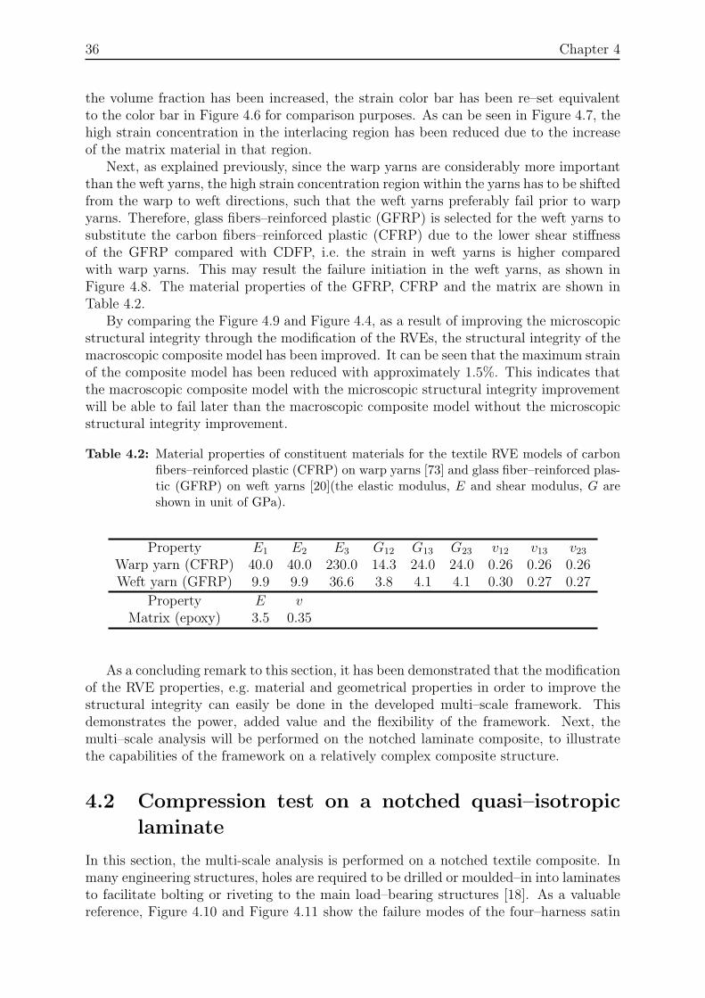
Next, as explained previously, since the warp yarns are considerably more importantthan the weft yarns, the high strain concentration region within the yarns has to be shiftedfrom the warp to weft directions, such that the weft yarns preferably fail prior to warpyarns. Therefore, glass fibers–reinforced plastic (GFRP) is selected for the weft yarns tosubstitute the carbon fibers–reinforced plastic (CFRP) due to the lower shear stiffnessof the GFRP compared with CDFP, i.e. the strain in weft yarns is higher comparedwith warp yarns. This may result the failure initiation in the weft yarns, as shown inFigure 4.8. The material properties of the GFRP, CFRP and the matrix are shown inTable 4.2.
By comparing the Figure 4.9 and Figure 4.4, as a result of improving the microscopicstructural integrity through the modification of the RVEs, the structural integrity of themacroscopic composite model has been improved. It can be seen that the maximum strainof the composite model has been reduced with approximately 1.5%. This indicates thatthe macroscopic composite model with the microscopic structural integrity improvementwill be able to fail later than the macroscopic composite model without the microscopicstructural integrity improvement.
Table 4.2: Material properties of constituent materials for the textile RVE models of carbonfibers–reinforced plastic (CFRP) on warp yarns [73] and glass fiber–reinforced plas-tic (GFRP) on weft yarns [20](the elastic modulus, E and shear modulus, G areshown in unit of GPa).
Property E1 E2 E3 G12 G13 G23 v12 v13 v23Warp yarn (CFRP) 40.0 40.0 230.0 14.3 24.0 24.0 0.26 0.26 0.26Weft yarn (GFRP) 9.9 9.9 36.6 3.8 4.1 4.1 0.30 0.27 0.27
Property E vMatrix (epoxy) 3.5 0.35
As a concluding remark to this section, it has been demonstrated that the modificationof the RVE properties, e.g. material and geometrical properties in order to improve thestructural integrity can easily be done in the developed multi–scale framework. Thisdemonstrates the power, added value and the flexibility of the framework. Next, themulti–scale analysis will be performed on the notched laminate composite, to illustratethe capabilities of the framework on a relatively complex composite structure.
4.2 Compression test on a notched quasi–isotropic
laminate
In this section, the multi-scale analysis is performed on a notched textile composite. Inmany engineering structures, holes are required to be drilled or moulded–in into laminatesto facilitate bolting or riveting to the main load–bearing structures [18]. As a valuablereference, Figure 4.10 and Figure 4.11 show the failure modes of the four–harness satin
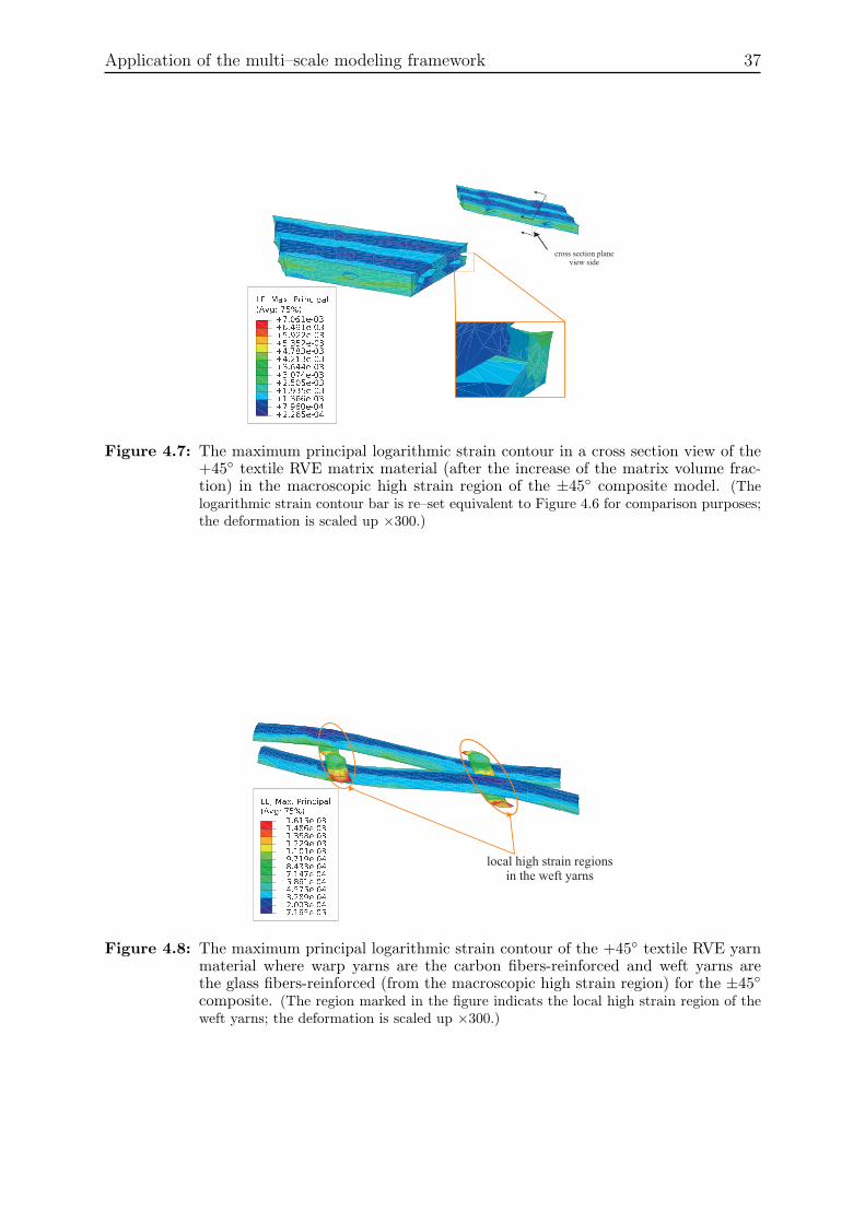
Application of the multi–scale modeling framework 37
cross section planeview side
Figure 4.7: The maximum principal logarithmic strain contour in a cross section view of the+45◦ textile RVE matrix material (after the increase of the matrix volume frac-tion) in the macroscopic high strain region of the ±45◦ composite model. (Thelogarithmic strain contour bar is re–set equivalent to Figure 4.6 for comparison purposes;the deformation is scaled up ×300.)
local high strain regionsin the weft yarns
Figure 4.8: The maximum principal logarithmic strain contour of the +45◦ textile RVE yarnmaterial where warp yarns are the carbon fibers-reinforced and weft yarns arethe glass fibers-reinforced (from the macroscopic high strain region) for the ±45◦
composite. (The region marked in the figure indicats the local high strain region of theweft yarns; the deformation is scaled up ×300.)
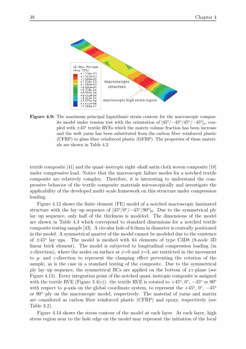
38 Chapter 4
macroscopic high strain region
macroscopicstructure
Figure 4.9: The maximum principal logarithmic strain contour for the macroscopic compos-ite model under tension test with the orientation of [45o/−45o/45o/−45o]s, cou-pled with ±45o textile RVEs which the matrix volume fraction has been increaseand the weft yarns has been substituted from the carbon fiber–reinforced plastic(CFRP) to glass fiber–reinforced plastic (GFRP). The properties of these materi-als are shown in Table 4.2.
textile composite [41] and the quasi–isotropic eight–shaft satin cloth woven composite [18]under compressive load. Notice that the macroscopic failure modes for a notched textilecomposite are relatively complex. Therefore, it is interesting to understand the com-pressive behavior of the textile composite materials microscopically and investigate theapplicability of the developed multi–scale framework on this structure under compressionloading.
Figure 4.12 shows the finite element (FE) model of a notched macroscopic laminatedstructure with the lay–up sequence of [45o/0o/−45o/90o]S. Due to the symmetrical plylay–up sequence, only half of the thickness is modeled. The dimensions of the modelare shown in Table 4.3 which correspond to standard dimensions for a notched textilecomposite testing sample [43]. A circular hole of 6.0mm in diameter is centrally positionedin the model. A symmetrical quarter of the model cannot be modeled due to the existenceof ±45o lay–ups. The model is meshed with 64 elements of type C3D8 (8-node 3Dlinear brick element). The model is subjected to longitudinal compression loading (inx-direction), where the nodes on surface at x=0 and x=L are restricted in the movementto y- and z-direction to represent the clamping effect preventing the rotation of thesample, as is the case in a standard testing of the composite. Due to the symmetricalply lay–up sequence, the symmetrical BCs are applied on the bottom of xz-plane (seeFigure 4.13). Every integration point of the notched quasi–isotropic composite is assignedwith the textile RVE (Figure 3.4(c)). the textile RVE is rotated to +45o, 0◦, −45o or 90o
with respect to y-axis on the global coordinate system, to represent the +45o, 0◦, −45o
or 90o–ply on the macroscopic model, respectively. The material of yarns and matrixare considered as carbon fiber–reinforced plastic (CFRP) and epoxy, respectively (seeTable 3.2).
Figure 4.14 shows the stress contour of the model at each layer. At each layer, highstress region near to the hole edge on the model may represent the initiation of the local
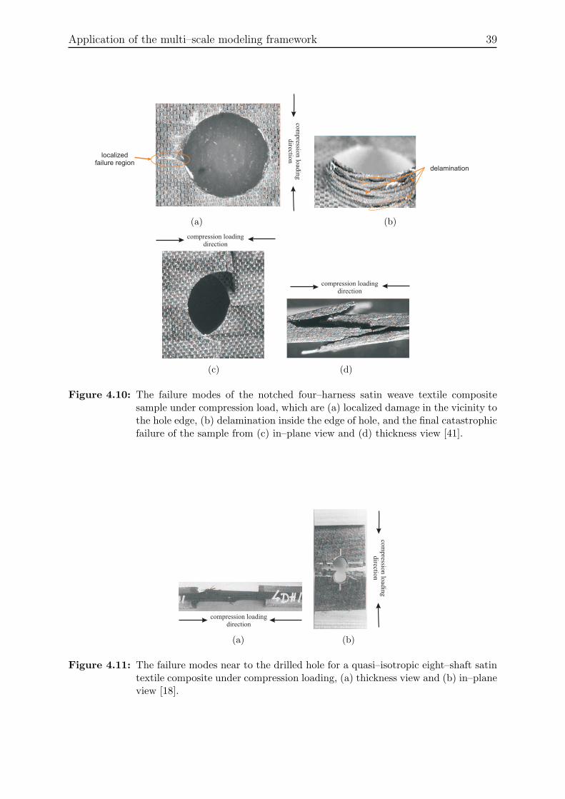
Application of the multi–scale modeling framework 39
localizedfailure region
com
pressio
n lo
adin
gdirectio
n
(a)
delamination
(b)
compression loadingdirection
(c)
compression loadingdirection
(d)
Figure 4.10: The failure modes of the notched four–harness satin weave textile compositesample under compression load, which are (a) localized damage in the vicinity tothe hole edge, (b) delamination inside the edge of hole, and the final catastrophicfailure of the sample from (c) in–plane view and (d) thickness view [41].
compression loadingdirection
(a)
com
pressio
n lo
adin
gdirectio
n
(b)
Figure 4.11: The failure modes near to the drilled hole for a quasi–isotropic eight–shaft satintextile composite under compression loading, (a) thickness view and (b) in–planeview [18].
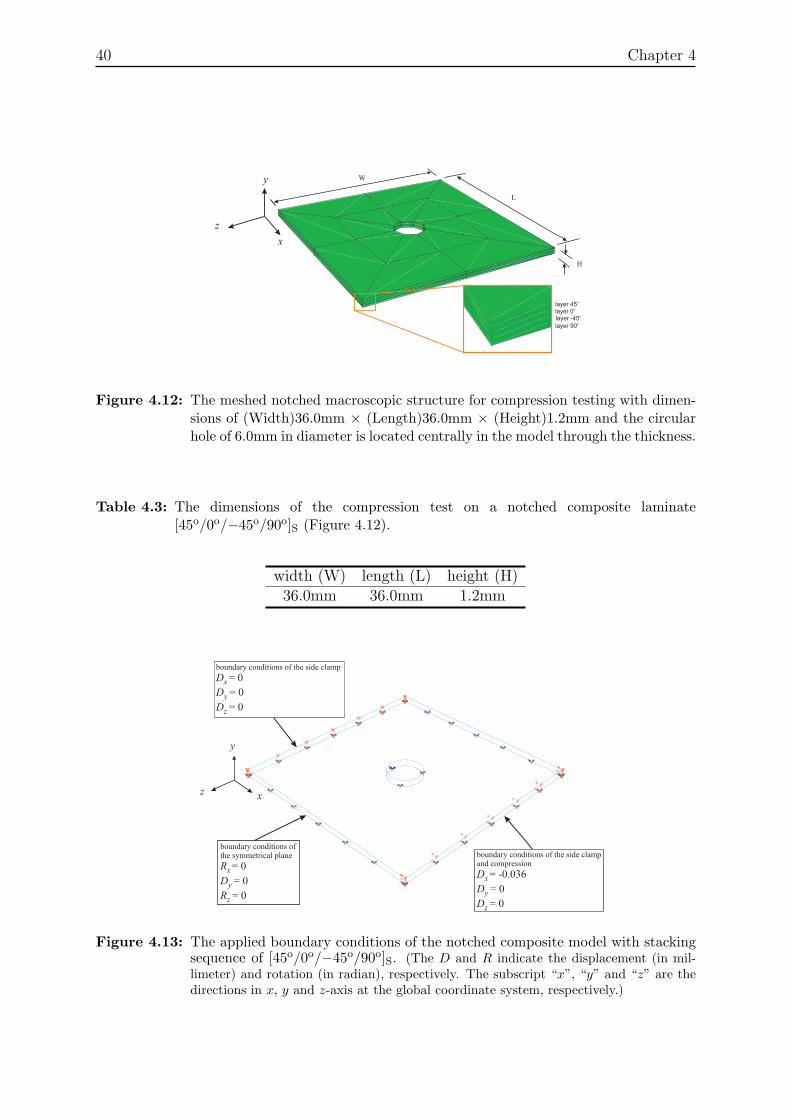
40 Chapter 4
y W
L
H
layer 45o
layer -45o
layer 0o
layer 90o
x
z
Figure 4.12: The meshed notched macroscopic structure for compression testing with dimen-sions of (Width)36.0mm × (Length)36.0mm × (Height)1.2mm and the circularhole of 6.0mm in diameter is located centrally in the model through the thickness.
Table 4.3: The dimensions of the compression test on a notched composite laminate[45o/0o/−45o/90o]S (Figure 4.12).
width (W) length (L) height (H)36.0mm 36.0mm 1.2mm
y
xz
boundary conditions of the side clampand compression
Dx = -0.036
D
Dy
z
= 0
= 0
boundary conditions of the side clamp
Dx = 0
D
Dy
z
= 0
= 0
boundary conditions ofthe symmetrical plane
Rx = 0
D
Ry
z
= 0
= 0
Figure 4.13: The applied boundary conditions of the notched composite model with stackingsequence of [45o/0o/−45o/90o]S. (The D and R indicate the displacement (in mil-limeter) and rotation (in radian), respectively. The subscript “x”, “y” and “z” are thedirections in x, y and z-axis at the global coordinate system, respectively.)
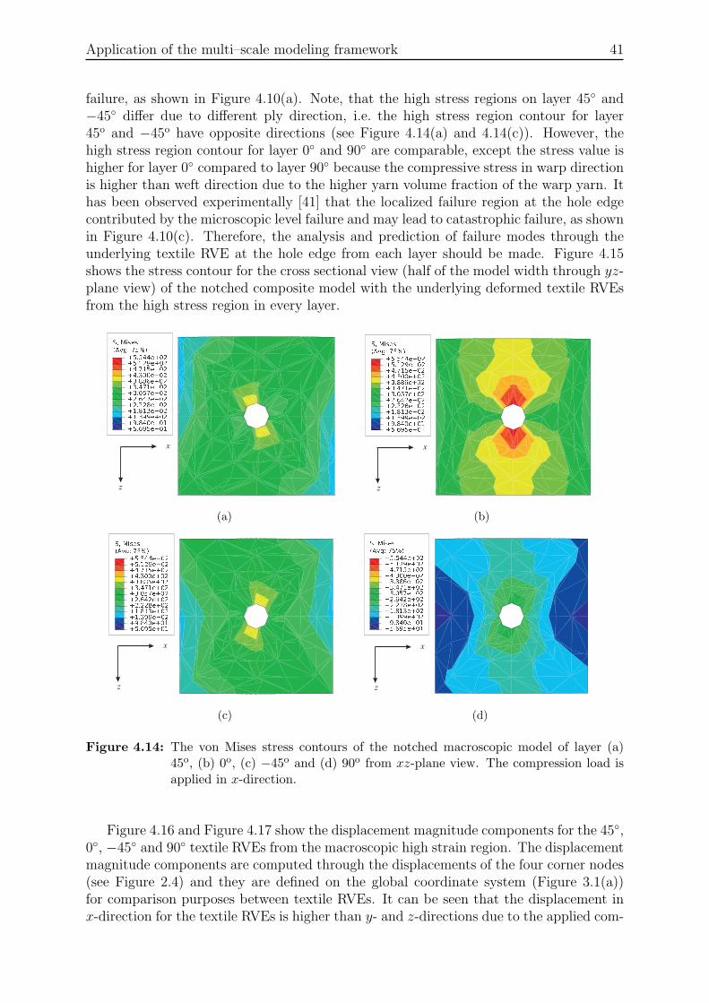
Application of the multi–scale modeling framework 41
failure, as shown in Figure 4.10(a). Note, that the high stress regions on layer 45◦ and−45◦ differ due to different ply direction, i.e. the high stress region contour for layer45o and −45o have opposite directions (see Figure 4.14(a) and 4.14(c)). However, thehigh stress region contour for layer 0◦ and 90◦ are comparable, except the stress value ishigher for layer 0◦ compared to layer 90◦ because the compressive stress in warp directionis higher than weft direction due to the higher yarn volume fraction of the warp yarn. Ithas been observed experimentally [41] that the localized failure region at the hole edgecontributed by the microscopic level failure and may lead to catastrophic failure, as shownin Figure 4.10(c). Therefore, the analysis and prediction of failure modes through theunderlying textile RVE at the hole edge from each layer should be made. Figure 4.15shows the stress contour for the cross sectional view (half of the model width through yz-plane view) of the notched composite model with the underlying deformed textile RVEsfrom the high stress region in every layer.
x
z
(a)
x
z
(b)
x
z
(c)
x
z
(d)
Figure 4.14: The von Mises stress contours of the notched macroscopic model of layer (a)45o, (b) 0o, (c) −45o and (d) 90o from xz-plane view. The compression load isapplied in x-direction.
Figure 4.16 and Figure 4.17 show the displacement magnitude components for the 45◦,0◦, −45◦ and 90◦ textile RVEs from the macroscopic high strain region. The displacementmagnitude components are computed through the displacements of the four corner nodes(see Figure 2.4) and they are defined on the global coordinate system (Figure 3.1(a))for comparison purposes between textile RVEs. It can be seen that the displacement inx-direction for the textile RVEs is higher than y- and z-directions due to the applied com-
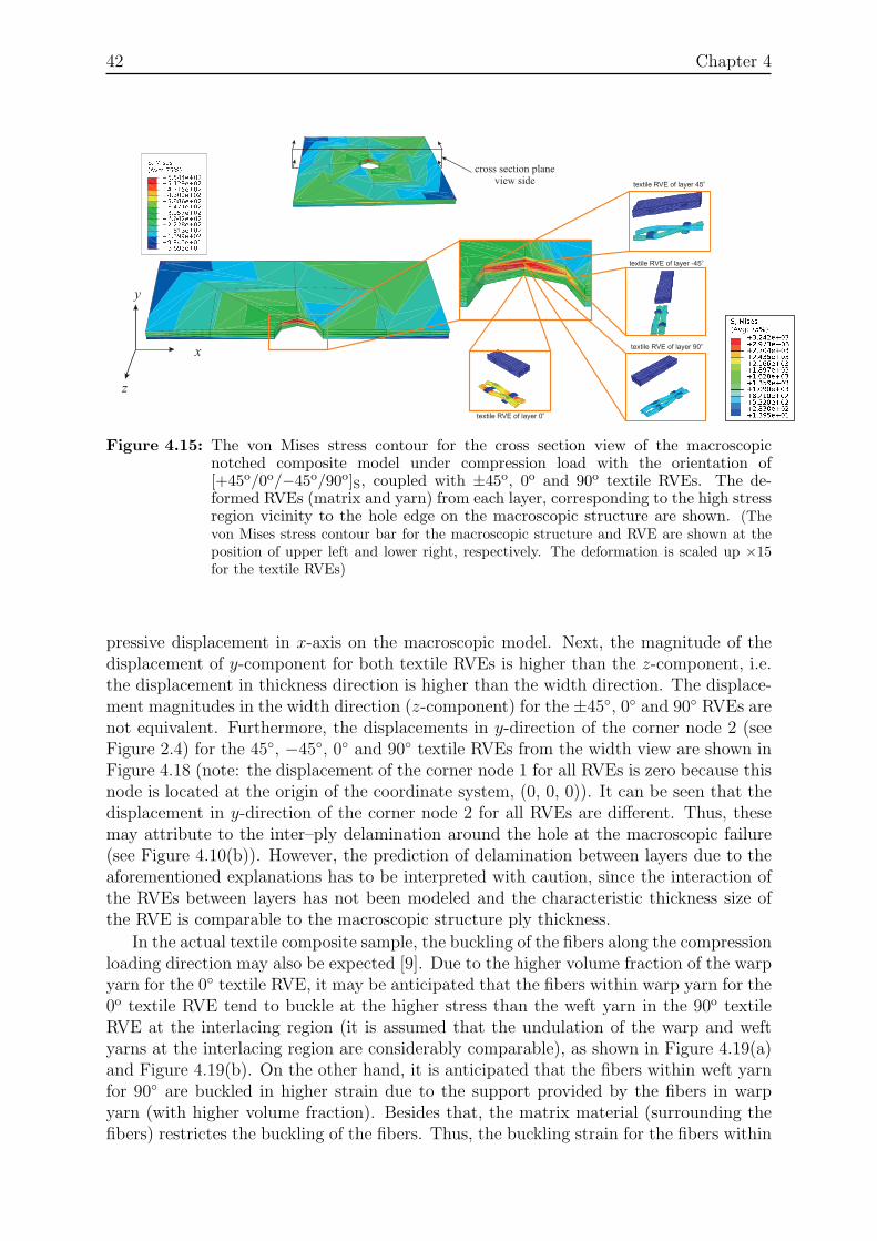
42 Chapter 4
textile RVE of layer 45o
textile RVE of layer 0o
textile RVE of layer -45o
textile RVE of layer 90o
x
z
y
cross section planeview side
Figure 4.15: The von Mises stress contour for the cross section view of the macroscopicnotched composite model under compression load with the orientation of[+45o/0o/−45o/90o]S, coupled with ±45o, 0o and 90o textile RVEs. The de-formed RVEs (matrix and yarn) from each layer, corresponding to the high stressregion vicinity to the hole edge on the macroscopic structure are shown. (Thevon Mises stress contour bar for the macroscopic structure and RVE are shown at theposition of upper left and lower right, respectively. The deformation is scaled up ×15for the textile RVEs)
pressive displacement in x-axis on the macroscopic model. Next, the magnitude of thedisplacement of y-component for both textile RVEs is higher than the z-component, i.e.the displacement in thickness direction is higher than the width direction. The displace-ment magnitudes in the width direction (z-component) for the ±45◦, 0◦ and 90◦ RVEs arenot equivalent. Furthermore, the displacements in y-direction of the corner node 2 (seeFigure 2.4) for the 45◦, −45◦, 0◦ and 90◦ textile RVEs from the width view are shown inFigure 4.18 (note: the displacement of the corner node 1 for all RVEs is zero because thisnode is located at the origin of the coordinate system, (0, 0, 0)). It can be seen that thedisplacement in y-direction of the corner node 2 for all RVEs are different. Thus, thesemay attribute to the inter–ply delamination around the hole at the macroscopic failure(see Figure 4.10(b)). However, the prediction of delamination between layers due to theaforementioned explanations has to be interpreted with caution, since the interaction ofthe RVEs between layers has not been modeled and the characteristic thickness size ofthe RVE is comparable to the macroscopic structure ply thickness.
In the actual textile composite sample, the buckling of the fibers along the compressionloading direction may also be expected [9]. Due to the higher volume fraction of the warpyarn for the 0◦ textile RVE, it may be anticipated that the fibers within warp yarn for the0o textile RVE tend to buckle at the higher stress than the weft yarn in the 90o textileRVE at the interlacing region (it is assumed that the undulation of the warp and weftyarns at the interlacing region are considerably comparable), as shown in Figure 4.19(a)and Figure 4.19(b). On the other hand, it is anticipated that the fibers within weft yarnfor 90◦ are buckled in higher strain due to the support provided by the fibers in warpyarn (with higher volume fraction). Besides that, the matrix material (surrounding thefibers) restrictes the buckling of the fibers. Thus, the buckling strain for the fibers within
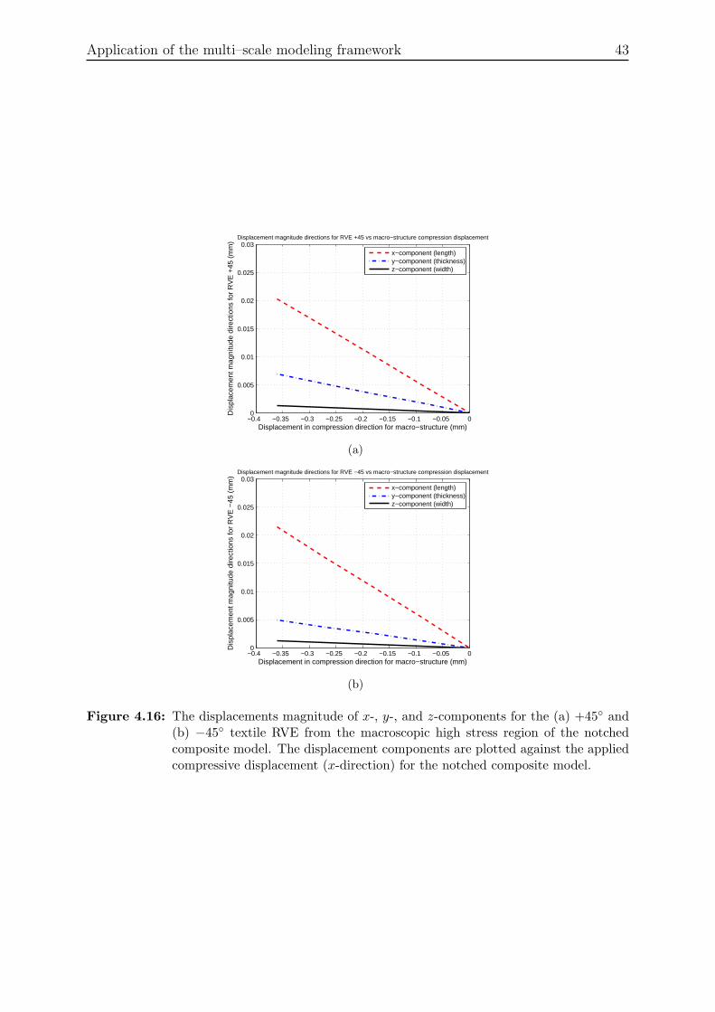
Application of the multi–scale modeling framework 43
−0.4 −0.35 −0.3 −0.25 −0.2 −0.15 −0.1 −0.05 00
0.005
0.01
0.015
0.02
0.025
0.03
Displacement in compression direction for macro−structure (mm)
Dis
plac
emen
t mag
nitu
de d
irect
ions
for
RV
E +
45 (
mm
)Displacement magnitude directions for RVE +45 vs macro−structure compression displacement
x−component (length)y−component (thickness)z−component (width)
(a)
−0.4 −0.35 −0.3 −0.25 −0.2 −0.15 −0.1 −0.05 00
0.005
0.01
0.015
0.02
0.025
0.03
Displacement in compression direction for macro−structure (mm)
Dis
plac
emen
t mag
nitu
de d
irect
ions
for
RV
E −
45 (
mm
)
Displacement magnitude directions for RVE −45 vs macro−structure compression displacement
x−component (length)y−component (thickness)z−component (width)
(b)
Figure 4.16: The displacements magnitude of x-, y-, and z-components for the (a) +45◦ and(b) −45◦ textile RVE from the macroscopic high stress region of the notchedcomposite model. The displacement components are plotted against the appliedcompressive displacement (x-direction) for the notched composite model.
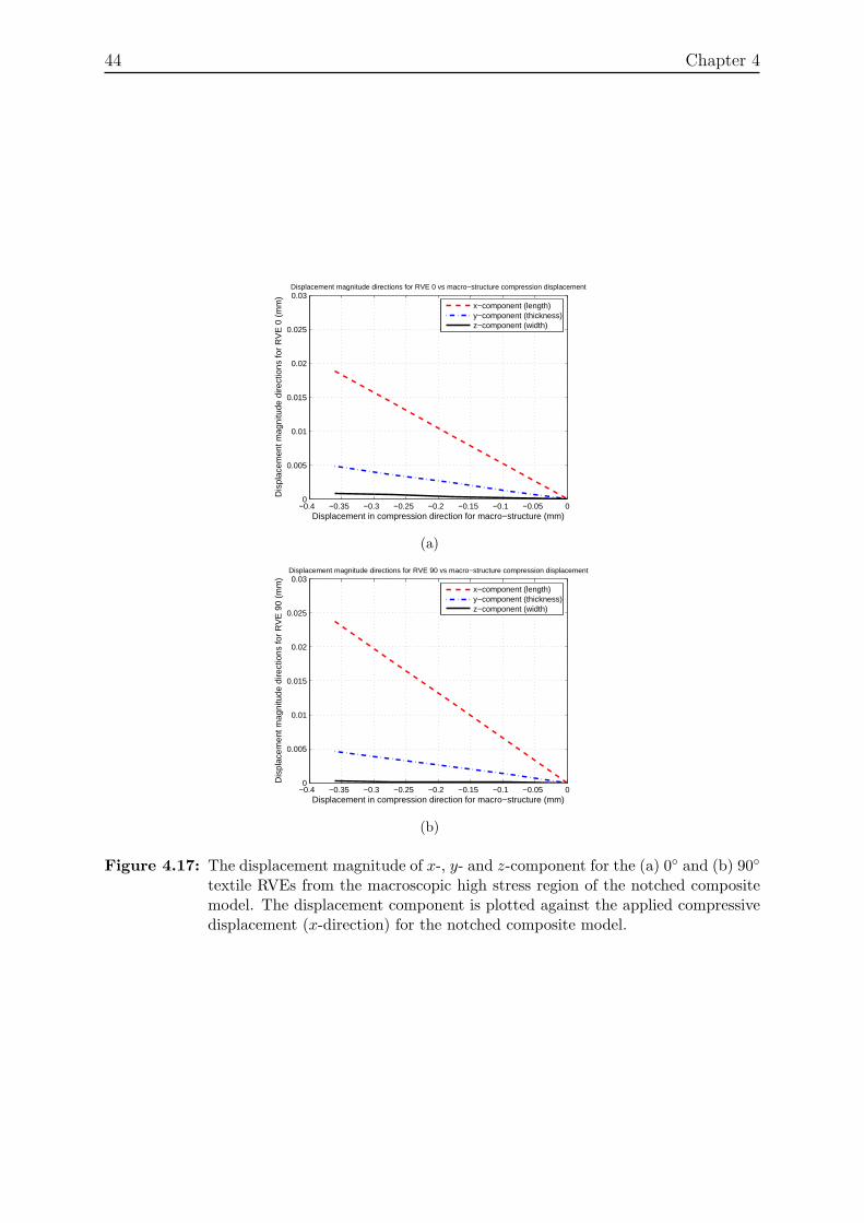
44 Chapter 4
−0.4 −0.35 −0.3 −0.25 −0.2 −0.15 −0.1 −0.05 00
0.005
0.01
0.015
0.02
0.025
0.03
Displacement in compression direction for macro−structure (mm)
Dis
plac
emen
t mag
nitu
de d
irect
ions
for
RV
E 0
(m
m)
Displacement magnitude directions for RVE 0 vs macro−structure compression displacement
x−component (length)y−component (thickness)z−component (width)
(a)
−0.4 −0.35 −0.3 −0.25 −0.2 −0.15 −0.1 −0.05 00
0.005
0.01
0.015
0.02
0.025
0.03
Displacement in compression direction for macro−structure (mm)
Dis
plac
emen
t mag
nitu
de d
irect
ions
for
RV
E 9
0 (m
m)
Displacement magnitude directions for RVE 90 vs macro−structure compression displacement
x−component (length)y−component (thickness)z−component (width)
(b)
Figure 4.17: The displacement magnitude of x-, y- and z-component for the (a) 0◦ and (b) 90◦
textile RVEs from the macroscopic high stress region of the notched compositemodel. The displacement component is plotted against the applied compressivedisplacement (x-direction) for the notched composite model.
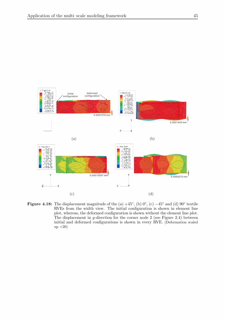
Application of the multi–scale modeling framework 45
X
Y
Z
0.0007279 mm
deformedconfiguration
initialconfiguration
(a)
0.0001425 mm
(b)
0.00015597 mm
(c)
0.0000275 mm
(d)
Figure 4.18: The displacement magnitude of the (a) +45◦, (b) 0◦, (c) −45◦ and (d) 90◦ textileRVEs from the width view. The initial configuration is shown in element lineplot, whereas, the deformed configuration is shown without the element line plot.The displacement in y-direction for the corner node 2 (see Figure 2.4) betweeninitial and deformed configurations is shown in every RVE. (Deformation scaledup ×20)
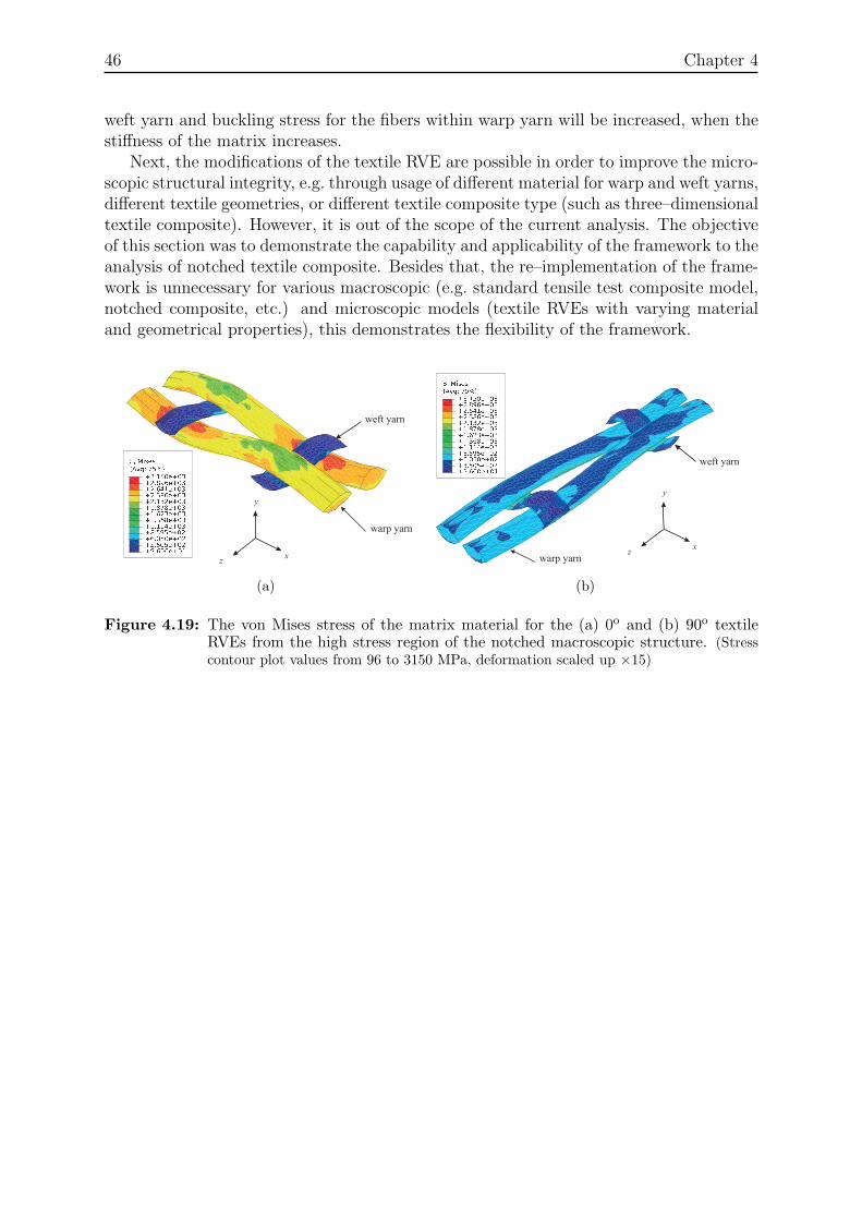
46 Chapter 4
weft yarn and buckling stress for the fibers within warp yarn will be increased, when thestiffness of the matrix increases.
Next, the modifications of the textile RVE are possible in order to improve the micro-scopic structural integrity, e.g. through usage of different material for warp and weft yarns,different textile geometries, or different textile composite type (such as three–dimensionaltextile composite). However, it is out of the scope of the current analysis. The objectiveof this section was to demonstrate the capability and applicability of the framework to theanalysis of notched textile composite. Besides that, the re–implementation of the frame-work is unnecessary for various macroscopic (e.g. standard tensile test composite model,notched composite, etc.) and microscopic models (textile RVEs with varying materialand geometrical properties), this demonstrates the flexibility of the framework.
y
xz
warp yarn
weft yarn
(a)
y
xz
warp yarn
weft yarn
(b)
Figure 4.19: The von Mises stress of the matrix material for the (a) 0o and (b) 90o textileRVEs from the high stress region of the notched macroscopic structure. (Stresscontour plot values from 96 to 3150 MPa, deformation scaled up ×15)
Chapter 5
Conclusions and recommendations
5.1 Conclusions
A framework for the multi–scale analysis of composite structures has been developedand performed. The advanced micro–mechanics modeling approach has been combinedthrough the computational homogenization with the structural analysis capabilities ofAbaqus with its subroutines. The Abaqus subroutines enable to link the macro– andmicro–scale composites structure analysis down to the level of the fiber (for unidirectionalcomposite materials), yarn (for textile composite materials) and matrix constituents ateach integration point for each macroscopic loading and iteration. As a result, the mecha-nisms of the microscopic composite materials in the macroscopic structure can be studiedin great detail collectively. Furthermore, the developed multi–scale computational ho-mogenization framework circumvents the need for complex and anisotropic constitutivemodels for composite materials analyses at the macroscopic and microscopic levels.
The correctness of the multi–scale framework for a heterogeneous material is demon-strated and tested by performing the analysis on the unidirectional fiber–reinforced mi-croscopic structure at the microscopic level analysis, as well as the macroscopic structure(coupled with the unidirectional fiber–reinforced microscopic structure) for the multi–scale analysis. The analysis results at both the microscopic level and the macroscopiclevel (from multi–scale analysis) are considerably good in agreement with the analyticalsolutions and the experimental data. Thus, the further multi–scale analyses on a rela-tively complex microscopic composite structure (e.g. textile composite) can be performedwith a great level of confidence.
Due to the unrealistic for the modeled microscopic plain weave textile composite, nocomparisons between the analysis results and experimental data are made. However, thesimulation results are compared with the tested textile composite sample qualitatively.In general, the prediction of the failure regions in the macroscopic composite model havebeen predicted correctly. Moreover, in the microscopic textile composite, the predictionsof the failure initiation in the matrix and the yarns which may contribute to the macro-scopic failure are made based on the local high stress or strain in the matrix or the yarns.The predictions are shown to be consistent with the simulation results and tested textilecomposite samples qualitatively from various research papers.
The multi–scale analysis example problems successfully demonstrated the applicabil-ity, power, added value and the flexibility of the developed multi–scale analysis frameworkto the analysis of textile composite structures. This development provides the opportu-nities for the engineer to re–design and improve the structural integrity of the composite
47
48 Chapter 5
structures, macroscopically and microscopically, without costly prototyping and testing.Therefore, this is one of the powerful and useful engineering tools for the future structuralanalysis and design.
5.2 Recommendations for future work
While the conclusions of the current work were presented in the previous section, severalrecommendations for further work will be discussed, as follow.
5.2.1 Multi–scale modeling framework
(i) The developed multi–scale framework only separates the structural length scaleinto macroscopic (comparable to composite test sample) and microscopic (compa-rable to the composite structure where the matrix constituent and yarn constituentcomposed of fibers and matrix, are distinguishable). However, the framework haspotential to be developed for the separation of macroscopic (comparable to com-posite test sample), microscopic (comparable to the composite structure where thematrix constituent and the yarn constituent composed of fibers and matrix are dis-tinguishable) and fiber–matrix level (comparable to the composite structure wherethe matrix and fibers are distinguishable) length scales, as shown in Figure 5.1.This separation of length scales is interesting to an engineer because in this waythe mechanical and material mechanisms of the structure can be predicted throughthe combination of different matrix and fiber materials from various suppliers be-fore placing the order of those materials. This should save the cost and time ofpurchasing, shipping, fabrication, testing and experimental post–processing.
(ii) The developed multi–scale modeling framework enables the study of the local macro-scopic mechanical and material behavior collectively. However, this approach isconsiderably computationally expensive in terms of time and computer memoryand hard–disk space because the multi–scale analysis at every integration point inthe macroscopic structure has to be performed at each macroscopic loading incre-ment and iteration. The advancement of the computer technologies, particularlythe speed of computing with the multi–core processor, has been improved signifi-cantly in the past decades, thus, the computational time of multi–scale analysis isexpected to reduce significantly in the future and it will become a worthy tool forthe engineers and scientists. However, several solutions can be proposed in order toimprove the computational efficiency even further.
(a) The selective method [19] can be performed using the failure criterion, while onthe non–critical regions (e.g. elastic region), the stiffness tangent obtained fromthe underlying RVEs can be kept constant throughout the analysis without per-forming the multi–scale analysis. In the critical region (e.g. the failure criterionis approaching the unity), the multi–scale analysis can be performed in orderto update the stiffness tangent. However, this method is unapplicable to theanalysis which interfacial delamination between the fibers and matrix is mod-eled (if the length scale separation shown in Figure 5.1 is simulated) becausethe macroscopic critical region where the interfacial delamination occurs is rel-
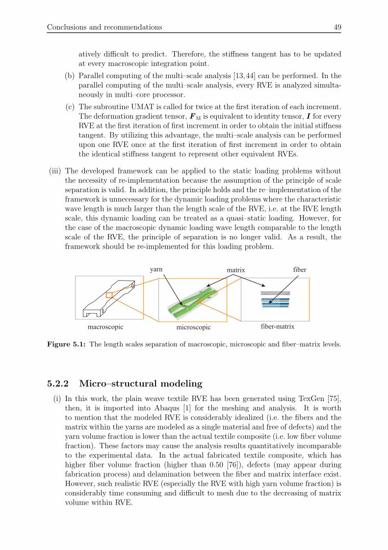
Conclusions and recommendations 49
atively difficult to predict. Therefore, the stiffness tangent has to be updatedat every macroscopic integration point.
(b) Parallel computing of the multi–scale analysis [13,44] can be performed. In theparallel computing of the multi–scale analysis, every RVE is analyzed simulta-neously in multi–core processor.
(c) The subroutine UMAT is called for twice at the first iteration of each increment.The deformation gradient tensor, FM is equivalent to identity tensor, I for everyRVE at the first iteration of first increment in order to obtain the initial stiffnesstangent. By utilizing this advantage, the multi–scale analysis can be performedupon one RVE once at the first iteration of first increment in order to obtainthe identical stiffness tangent to represent other equivalent RVEs.
(iii) The developed framework can be applied to the static loading problems withoutthe necessity of re-implementation because the assumption of the principle of scaleseparation is valid. In addition, the principle holds and the re–implementation of theframework is unnecessary for the dynamic loading problems where the characteristicwave length is much larger than the length scale of the RVE, i.e. at the RVE lengthscale, this dynamic loading can be treated as a quasi–static loading. However, forthe case of the macroscopic dynamic loading wave length comparable to the lengthscale of the RVE, the principle of separation is no longer valid. As a result, theframework should be re-implemented for this loading problem.
yarn matrix fiber
macroscopic microscopic fiber-matrix
Figure 5.1: The length scales separation of macroscopic, microscopic and fiber–matrix levels.
5.2.2 Micro–structural modeling
(i) In this work, the plain weave textile RVE has been generated using TexGen [75],then, it is imported into Abaqus [1] for the meshing and analysis. It is worthto mention that the modeled RVE is considerably idealized (i.e. the fibers and thematrix within the yarns are modeled as a single material and free of defects) and theyarn volume fraction is lower than the actual textile composite (i.e. low fiber volumefraction). These factors may cause the analysis results quantitatively incomparableto the experimental data. In the actual fabricated textile composite, which hashigher fiber volume fraction (higher than 0.50 [76]), defects (may appear duringfabrication process) and delamination between the fiber and matrix interface exist.However, such realistic RVE (especially the RVE with high yarn volume fraction) isconsiderably time consuming and difficult to mesh due to the decreasing of matrixvolume within RVE.
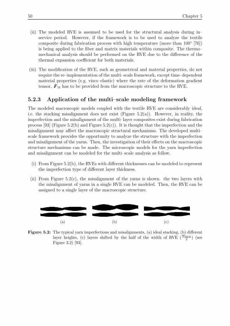
50 Chapter 5
(ii) The modeled RVE is assumed to be used for the structural analysis during in–service period. However, if the framework is to be used to analyze the textilecomposite during fabrication process with high temperature (more than 100◦ [76])is being applied to the fiber and matrix materials within composite. The thermo–mechanical analysis should be performed on the RVE due to the difference of thethermal expansion coefficient for both materials.
(iii) The modification of the RVE, such as geometrical and material properties, do notrequire the re–implementation of the multi–scale framework, except time–dependentmaterial properties (e.g. visco–elastic) where the rate of the deformation gradienttensor, FM has to be provided from the macroscopic structure to the RVE.
5.2.3 Application of the multi–scale modeling framework
The modeled macroscopic models coupled with the textile RVE are considerably ideal,i.e. the stacking misalignment does not exist (Figure 5.2(a)). However, in reality, theimperfection and the misalignment of the multi–layer composites exist during fabricationprocess [93] (Figure 5.2(b) and Figure 5.2(c)). It is thought that the imperfection and themisalignment may affect the macroscopic structural mechanisms. The developed multi–scale framework provides the opportunity to analyze the structure with the imperfectionand misalignment of the yarns. Then, the investigation of their effects on the macroscopicstructure mechanisms can be made. The microscopic models for the yarn imperfectionand misalignment can be modeled for the multi–scale analysis as follow.
(i) From Figure 5.2(b), the RVEs with different thicknesses can be modeled to representthe imperfection type of different layer thickness.
(ii) From Figure 5.2(c), the misalignment of the yarns is shown. the two layers withthe misalignment of yarns in a single RVE can be modeled. Then, the RVE can beassigned to a single layer of the macroscopic structure.
(a) (b) (c)
Figure 5.2: The typical yarn imperfections and misalignments, (a) ideal stacking, (b) differentlayer heights, (c) layers shifted by the half of the width of RVE (WRVE
2 ) (seeFigure 3.2) [93].
Bibliography
[1] Abaqus/standard version 6.9. Analysis user’s manuals. developed by HKS Inc. ofRhone Island, USA and marketed under SIMULIA brand of Dassault Systemes S.A.,2009.
[2] M. Bannister. Development and application of advanced textile composites. Pro-
ceedings of the Institution of Mechanical Engineers, Part L: Journal of Materials:
Design and Applications, 218:253–260, 2004.
[3] D. Bigaud and P. Hamelin. Stiffness and failure modeling of 2D and 3D textile–reinforced composites by means of imbricates–type elements approaches. Computers
and Structures, 80:2253–2264, 2002.
[4] P. Boisse, A. Gasser, and G. Hivet. Analyses of fabric tensile behaviour: determi-nation of the biaxial tension strain surfaces and their use in forming simulations.Composites Part A: Applied Science and Manufacturing, 32:1395–1414, 2001.
[5] C. Chamis. Simplified composite micromechanics equations for hygral, thermal andmechanical properties. Society for the Advancement of Material and Process Engi-
neering, April:14–23, 1984.
[6] R. Christensen. A critical evaluation for a class of micromechanics models. Journalof the Mechanics and Physics of Solids, 38:379–404, 1990.
[7] T. Chua. A framework for performing multi–scale analysis on composite usingabaqus. Technical report, Fokker Landing Gear B.V., Helmond, The Netherlands,October 2010.
[8] P. Chung, K. Tamma, and R. Namburu. Asymptotic expansion homogenization forheterogeneous media: computational issues and applications. Composite: Part A,32:1291–1301, 2001.
[9] B. Cox, M. DadKhah, W. Morris, and J. Flintoff. Failure mechanisms of 3D wovencomposites in tension, compression and bending. Acta Metallurgica et Materialia,12:3967–3984, 1994.
[10] B. N. Cox and G. Flanagan. Handbook of Analytical Methods for Textile Com-posites. Contractor Report 4750, National Aeronautical and Space Administration(NASA), March 1997. Prepared for Langley Research Center under Contract NAS1-19243.
[11] S. Demiray, W. Becker, and J. Hohe. Analysis of two– and three–dimensional hy-perelastic model foams under complex loading conditons. Mechanics of Materials,38:985–1000, 2006.
51
52 Bibliography
[12] J. Eshelby. The determination of the field of an ellipsoidal inclusion and relatedproblems. Proceeding of the Royal Society A: Mathematical, Physical & Engineering
Sciences, 241:376–396, 1957.
[13] F. Feyel and J. Chaboche. FE2 multiscale approach for modelling the elastovis-coplastic behaviour of long fiber SiC/Ti composite materials. Computer Methods in
Applied Mechanics and Engineering, 183:309–330, 2000.
[14] E. Fredrik, M. David, A. Leif E., and J. Varna. Formation of damage and its effectson non-crimp fabric reinforced composites loaded in tension. Composite Science and
Technology, 64:675–692, 2004.
[15] V. Ganesh and N. Naik. Failure behaviour of plain weave fabric laminates underin–plane shear loading: effect of fabric geometry. Composite Structures, 30:179–192,1995.
[16] M. Geers, E. Coenen, and V. Kouznetsova. Multi–scale computational homogeniza-tion of structural thin sheets. Modeling and Simulation in Materials Science and
Engineering, 15:S393–S404, 2007.
[17] M. Geers, V. Kouznetsova, and W. Brekelmans. Multi–scale computational homoge-nization: trends and challenges. Journal of Computational and Applied Mathematics,2009.
[18] M. Ghasemi Nejhad and T. Chou. Compresssion behavior of woven carbon fibre–reinforced epoxy composites with moulded–in and drilled holes. Composites, 21:33–40, 1990.
[19] S. Ghosh, K. Lee, and P. Raghavan. A multi–level computational model for multi–scale damage analysis in composite and porous materials. International Journal of
Solids and Structures, 38:2335–2385, 2001.
[20] E. Glaessgen, C. Pastore, O. Griffin, and A. Birger. Geometrical and finite elementmodelling of textile composites. Composites: Part B, 27:43–50, 1996.
[21] B. Gommers, I. Verpoest, and P. van Houtte. The Mori–Tanaka method applied totextile composite materials. Acta Materiallia, 46:2223–2235, 1998.
[22] Z. Hashin. The elastic moduli of heterogeneous materials. Journal of Applied Me-
chanics, 50:481–505, 1962.
[23] Z. Hashin and B. Rosen. The elastic moduli of fiber–reinforced materials. American
Society of Mechanical Engineers, 31:223–232, 1964.
[24] J. Hearle. Engineering design of textiles. Indian Journal of Fibres and Textile,31:142–149, 2006.
[25] R. Hill. Elastic properties of reinforced solids some theoretical principles. Journal
of the Mechanics and Physics of Solids, 11:357–372, 1963.
[26] R. Hill. On constitutive macro-variables for heterogeneous solids at finite strain.Proceedings of the Royal Society of London. Series A, Mathematical and Physical,326(1565):131–147, 1972.
Bibliography 53
[27] T. Ishikawa and T. Chou. Elastic behavior of woven hybrid composite. Journal of
Materials Science, 16:2–19, 1982.
[28] T. Ishikawa and T. Chou. Nonlinear behavior of woven fabric composites. Computers
& Structures, 17:399–413, 1983.
[29] T. Ishikawa and T. Chou. One–dimensional micromechanical analysis of woven fabriccomposites. AIAA, 21:1714–1721, 1983.
[30] M. Ito and T. Chou. Elastic moduli and stress field of plain–weave composites undertensile loading. Composites Science and Technology, 57:787–800, 1997.
[31] I. Ivanov and A. Tabiei. Three–dimensional computational micro–mechanical modelfor woven fabric composites. Composites Structures, 54:489–496, 2001.
[32] R. Kamiya, R. Cheeseman, P. Popper, and T. Chou. Some recent advances in thefabrication and design of three–dimensional textile preforms: a review. Composites
Science and Technology, 60:33–47, 2000.
[33] R. Karkkainen and B. Sankar. A direct micromechanics method for analysis of failureinitiation of plain weave textile composites. Composites Science and Technology,66:137–150, 2006.
[34] R. L. Karkkainen, B. V. Sankar, and T. T. Jerome. Strength prediction of multi–layerplain weave textile composites using the direct micromechanics method. Composites:
Part B, 38:924–932, 2007.
[35] D. Kenaga, J. Doyle, and C. Sun. The characterization of boron/aluminum in thenonlinear range as an orthotropic elastic plastic material. Journal of Composite
Materials, 27:516–531, 1987.
[36] M. King, P. Jearanaisilawong, and S. Socrate. A continuum constitutive modelfor the mechanical behavior of woven fabrics. International Journal of Solids and
Structures, 42:3867–3896, 2005.
[37] V. Kouznetsova. Computational homogenization for the multi–scale of multi–phase
materials. PhD thesis, Eindhoven University of Technology, The Netherlands, 2002.
[38] V. Kouznetsova, W. Brekelmens, and F. Baaijens. An approach to micro–macromodeling of heterogeneous materials. Computational Mechanics, 27:37–48, 2001.
[39] V. Kouznetsova, M. Geers, and W. Brekelmans. Multi–scale second–order compu-tational homogenization of heterogeneous materials. ICTAM, XXI:15–21, 2004.
[40] S. Lomov, I. Verpoest, T. Peeters, D. Roose, and M. Zako. Nesting in textile lam-inates: geometrical modeling of the laminate. Composites Science and Technology,63:993–1007, 2003.
[41] S. Mall, D. Katwyk, R. Bolick, A. Kelkar, and D. Davis. Tension–compression fa-tigue behavior of a H–VARTM manufactured unnotched and notched carbon/epoxycomposite. Composite Structures, 90:201–207, 2009.
54 Bibliography
[42] R. Marrey and B. Sankar. Micromechanical models for textile structural composites.Technical Report 198229, National Aeronautical and Space Administration (NASA),Langley Research Center, Hampton, Virginia, 1995.
[43] J. E. Masters and M. A. Portanova. Standard test methods for textile composites.Lockheed Martin Engineering and Science Company, Hampton, Virginia, US, Con-tract NASI-19000 edition, September 1996. NASA Contractors Report 4751.
[44] K. Matsui, K. Terada, and K. Yuge. Parallelized two–scale analysis with a PC clus-ter for elastic–plastic heterogeneous media. Japan Society Mechanical Engineering
International Journal Series A, 44:584–593, 2001.
[45] W. Micheal Lai, D. Rubin, and E. Krempl. Introduction to Continuum Mechanics.Butterworth Heinemann, 3rd edition, 1993.
[46] J. Michel, H. Moulinec, and P. Suquet. Effective properties of composite materialswith periodic microstructure: a computational approach. Computer Methods in
Applied Mechanics and Engineering, 172:109–143, 1999.
[47] C. Miehe. Strain–driven homogenization of inelastic microstructures and compositesbased on an incremental variational formulation. International Journal for Numerical
Methods in Engineering, 55:1285–1322, 2002.
[48] C. Miehe. Computational micro–to–macro transitions for discretized micro–structures of heterogeneous materials at finite strains based on the minimizationof averaged incremental energy. Computer Methods in Applied Mechanics and En-
gineering, 192:559–591, 2003.
[49] C. Miehe and A. Koch. Computational micro–to–macro transition of discretizedmicrostructures undergoing small strain. Archive of Applied Mechanics, 72:300–317,2002.
[50] C. Miehe, J. Schroder, and M. Becker. Computational homogenization analysisin finite elasticity: material and structural instabilities on the micro– and macro–scales of periodic composites and their interaction. Computer Methods in Applied
Mechanics and Engineering, 191:4971–5005, 2002.
[51] T. Mori and K. Tanaka. Average stress in the matrix and average elastic energy ofmaterials with misfitting inclusions. Acta Metallurgica, 21:571–574, 1973.
[52] H. Moulinec and P. Suquet. Numerical method for computing the overall responseof nonlinear composites with complex microstructure. Computer Methods in Applied
Mechanics and Engineering, 157:69–94, 1998.
[53] A. Mouritz, M. Bannister, P. Falzon, and K. Leong. Review of applications foradvanced three–dimensional fibre textile composites. Composites: Part A, 30:1445–1461, 1999.
[54] K. Naik and V. Ganesh. Prediction of on–axes elastic properties of plain weave fabriccomposites. Composites Science and Technology, 45:135–152, 1992.
[55] N. Naik and P. Shembekar. Elastic behavior of woven fabric composites: I–laminaanalysis. Journal of Composite Materials, 26:2197–2225, 1992.
Bibliography 55
[56] N. Naik and P. Shembekar. Elastic behavior of woven fabric composites: III–laminatedesign. Journal of Composite Materials, 26:2523–2541, 1992.
[57] G. Nicoletto and R. Enrica. Failure mechanicsms in twill–weave laminates: FEMpredictions vs. experiments. Composites: Part A, 35:787–795, 2004.
[58] S. D. Pandita, G. Huysmans, M. Wevers, and Verpoest. Tensile fatigue behaviourof glass plain–weave fabric composites in on– and off–axis directions. Composites:
Part A, 32:1533–1539, 2001.
[59] P. Potluri and V. Thammandra. Influence of uniaxial and biaxial tension on meso-scale geometry and strain fields in a woven composite. Composites Structures,77:405–418, 2007.
[60] P. Rupnowski, M. Gentz, J. Sutter, and M. Kumosa. Mechanical response of awoven graphite/polyimide composite to in-plane shear dominated loads at room andelevated temperatures. Acta Materialia, 74:5603–5613, 2004.
[61] P. Shembekar and N. Naik. Elastic behavior of woven fabric composites: II–laminateanalysis. Journal of Composite Materials, 26:2226–2246, 1992.
[62] P. Shembekar and N. Naik. Notched strength of fabric laminates. II: Effect of stackingsequence. Composites Science and Technology, 44:13–20, 1992.
[63] M. Sherburn. Geometric and mechanical modelling of textiles. PhD thesis, TheUniversity of Nottingham, England, 2007.
[64] S. Sihn, E. V. Iarve, and A. K. Roy. Three–dimensional stress analysis of textile com-posites: Part I. Numerical analysis. International Journal of Solids and Structures,41:1377–1393, 2004.
[65] S. Sihn and A. Roy. Development of a three–dimensional mixed variational modelfor woven composites. II numerical solution and validation. International Journal ofSolids and Structures, 38:5949–5962, 2001.
[66] K. Srirengan, J. Whitcomb, and C. Chapman. Modal technique for three–dimensional global/local stress analysis of plain weave composites. Composite Struc-
tures, 39:145–156, 1997.
[67] C. Sun and R. Vaidya. Prediction of composite properties from a representativevolume element. Composites Science and Technology, 56:171–179, 1996.
[68] P. Suquet. Local and global aspects in the mathematical theory of plasticity. Plas-ticity Today: Modelling, Methods and Applications, pages 279–310, 1985.
[69] P. Suquet. Overall potentials and extremal surfaces of power law or ideally plasticcomposites. Journal of the Mechanics and Physics of Solids, 41:981–1002, 1993.
[70] A. Tabiei and Y. Jiang. Woven fabric composite material model with material non-linearity for nonlinear finite element simulation. International Journal of Solids andStructures, 36:2757–2771, 1999.
56 Bibliography
[71] A. Tabiei and W. Yi. Comparative study of predictive methods for woven fabriccomposite elastic properties. Composite Structures, 58:149–164, 2002.
[72] N. Takano, Y. Uetsuji, Y. Kashiwagi, and M. Zako. Hierarchical modelling of textilecomposite materials and structures by the homogenization method. Modelling and
Simulation in Materials Science and Engineering, 7:207–231, 1999.
[73] P. Tan, L. Tong, and G. Steven. A three–dimensional modelling technique for predict-ing the linear elastic property of opened–packing woven fabric unit cells. Composite
Structures, 38:261–271, 1997.
[74] K. Terada, M. Hori, T. Kyoya, and N. Kikuchi. Simulation of the multi–scale conver-gence in computational homogenization approaches. International Journal of Solidsand Structures, 37:2285–2311, 2000.
[75] TexGen version 3.3.0. TexGen textile composites modeling preprocessor user’s guide
manuals. developed at the University of Nottingham, UK and licensed under theGeneral Public License, 2008.
[76] B. Thuis. The development of composite landing gear components for aerospaceapplications. unclassified NLR–TP–2004–141, Nationaal Lucht–en Ruimtevaartlab-oratorium (NLR), The Netherlands, April 2004.
[77] O. van der Sluis, P. B. W. Schreurs, and H. Meijer. Overall behaviour of heteroge-neous elastoviscoplastic materials: effect of microstructural modelling. Mechanics of
Materials, 32:449–462, 2000.
[78] M. van Gils, O. van der Sluis, G. Zhang, J. Janssen, and R. Voncken. Analysis ofCu/low–k bond pad delamination by using a novel failure index. Microelectronics
Reliability, 47:179–186, 2007.
[79] P. Vandeurzen, J. Ivens, and I. Verpoest. A three–dimensional micromechanicalanalysis of woven–fabric composites: I. Geometric analysis. Composites Science and
Technology, 56:1303–1315, 1996.
[80] P. Vandeurzen, J. Ivens, and I. Verpoest. A three–dimensional micromechanicalanalysis of woven–fabric composites: II. Elastic analysis. Composites Science and
Technology, 56:1317–1327, 1996.
[81] M. Venkat Rao, P. Mahajan, and R. Mittal. Effect of architecture on mechanicalproperties of carbon–carbon composites. Composite Structures, 83:131–142, 2008.
[82] I. Verpoest and S. Lomov. Virtual textile composites software wisetex: Integrationwith micro–mechanical, permeability and structural analysis. Composites Science
and Technology, 65:2563–2574, 2005.
[83] X. Wang, B. Hu, Y. Feng, F. Liang, J. Mo, J. Xiong, and Y. Qiu. Low velocity impactproperties of 3D woven basalt/aramid hybrid composites. Composites Science and
Technology, 68:444–450, 2008.
[84] X. Wang, X. Wang, G. Zhou, and C. Zhou. Multi–scale analyses of 3D woven com-posite based on periodicity boundary conditions. Journal of Composite Materials,41:1773–1788, 2007.
Bibliography 57
[85] J. Whitcomb. Iterative global/local finite element analysis. Computers & Structures,40:1027–1032, 1991.
[86] J. Whitcomb, K. Srirengan, and C. Chapman. Evaluation of homogenization forglobal/local stress analysis of textile composites. Composite Structures, 31:137–149,1995.
[87] C. Wong, A. Long, M. Sherburn, F. Robitaille, P. Harrison, and C. Rudd. Compari-son of novel and efficient approaches for permeability prediction based on the fabricarchitecture. Composites: Part A, 37:847–857, 2006.
[88] K. Woo and J. D. Whitcomb. A post–processsor approach for stress analysis ofwoven textile composites. Composites Science and Technology, 60:693–704, 2000.
[89] Z. Wu. Three–dimensional exact modeling of geometric and mechanical propertiesof woven composites. Acta Mechanica Solids Sinica, 22:479–486, 2009.
[90] Y. Xu, W. Zhang, and D. Bassir. Stress analysis of multi–phase and multi–layer plainweave composite structure using global/local approach. Composites Structures, 2009.
[91] Y. Yeong Moo, P. Sang Hoon, and Y. Sung Kie. Asymptotic homogenization ofviscoelastic composites with periodic microstructures. International Journal of Solidsand Structures, 35(17):2039–2055, 1998.
[92] M. Zako, T. Uetsuji, and T. Kurashiki. Finite element analysis of damaged wovenfabric composite materials. Composite Science and Technology, 63:507–516, 2003.
[93] J. Zeman and M. Sejnoha. Homogenization of balanced plain weave composites withimperfect microstructure: Part I – Theoretical formulation. International Journal
of Solids and Structures, 41:6549–6571, 2004.
[94] Y. Zhang and J. Harding. A numerical micromechanics analysis of the mechanicalproperties of a plain weave composite. Computers & Structures, 36:839–844, 1990.
[95] L. Zhao, N. Warrior, and A. Long. Finite element modelling of damage progression innon-crimp fabric reinforced composites. Composite Science and Technology, 66:36–50, 2006.

Appendices
58
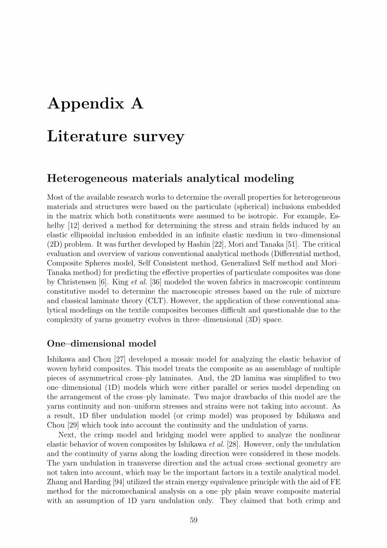
Appendix A
Literature survey
Heterogeneous materials analytical modeling
Most of the available research works to determine the overall properties for heterogeneousmaterials and structures were based on the particulate (spherical) inclusions embeddedin the matrix which both constituents were assumed to be isotropic. For example, Es-helby [12] derived a method for determining the stress and strain fields induced by anelastic ellipsoidal inclusion embedded in an infinite elastic medium in two–dimensional(2D) problem. It was further developed by Hashin [22], Mori and Tanaka [51]. The criticalevaluation and overview of various conventional analytical methods (Differential method,Composite Spheres model, Self Consistent method, Generalized Self method and Mori–Tanaka method) for predicting the effective properties of particulate composites was doneby Christensen [6]. King et al. [36] modeled the woven fabrics in macroscopic continuumconstitutive model to determine the macroscopic stresses based on the rule of mixtureand classical laminate theory (CLT). However, the application of these conventional ana-lytical modelings on the textile composites becomes difficult and questionable due to thecomplexity of yarns geometry evolves in three–dimensional (3D) space.
One–dimensional model
Ishikawa and Chou [27] developed a mosaic model for analyzing the elastic behavior ofwoven hybrid composites. This model treats the composite as an assemblage of multiplepieces of asymmetrical cross–ply laminates. And, the 2D lamina was simplified to twoone–dimensional (1D) models which were either parallel or series model depending onthe arrangement of the cross–ply laminate. Two major drawbacks of this model are theyarns continuity and non–uniform stresses and strains were not taking into account. Asa result, 1D fiber undulation model (or crimp model) was proposed by Ishikawa andChou [29] which took into account the continuity and the undulation of yarns.
Next, the crimp model and bridging model were applied to analyze the nonlinearelastic behavior of woven composites by Ishikawa et al. [28]. However, only the undulationand the continuity of yarns along the loading direction were considered in these models.The yarn undulation in transverse direction and the actual cross–sectional geometry arenot taken into account, which may be the important factors in a textile analytical model.Zhang and Harding [94] utilized the strain energy equivalence principle with the aid of FEmethod for the micromechanical analysis on a one–ply plain weave composite materialwith an assumption of 1D yarn undulation only. They claimed that both crimp and
59
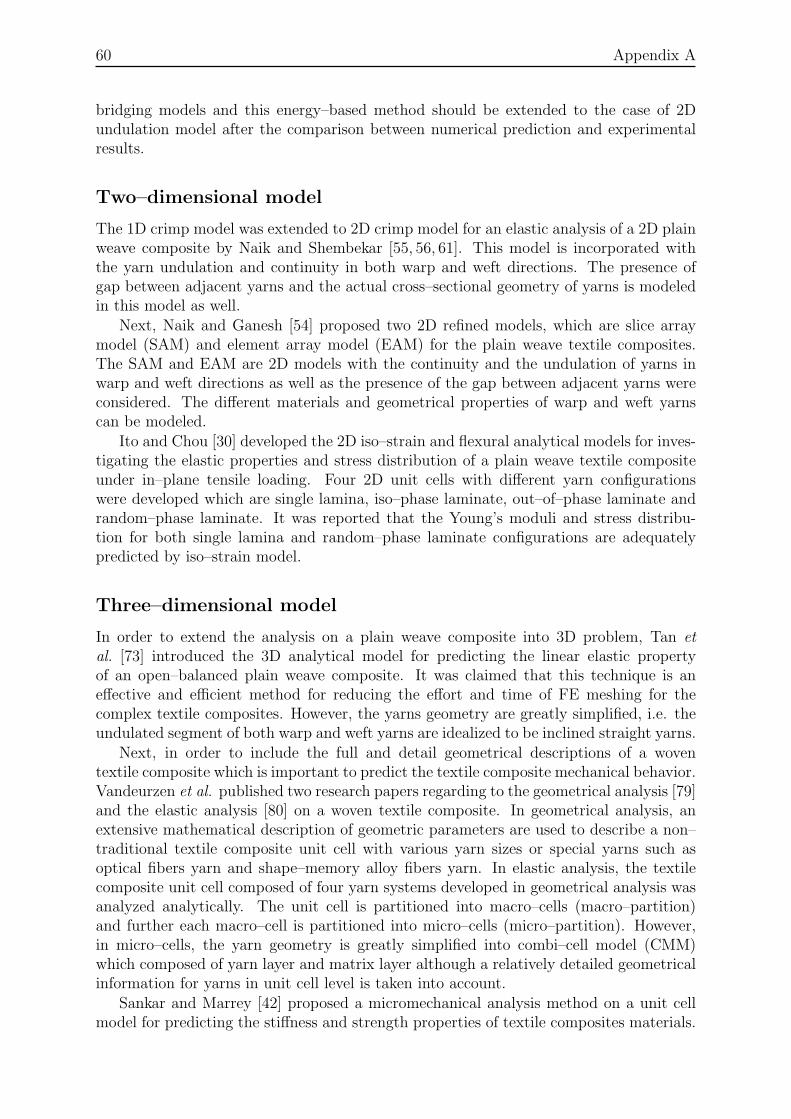
60 Appendix A
bridging models and this energy–based method should be extended to the case of 2Dundulation model after the comparison between numerical prediction and experimentalresults.
Two–dimensional model
The 1D crimp model was extended to 2D crimp model for an elastic analysis of a 2D plainweave composite by Naik and Shembekar [55, 56, 61]. This model is incorporated withthe yarn undulation and continuity in both warp and weft directions. The presence ofgap between adjacent yarns and the actual cross–sectional geometry of yarns is modeledin this model as well.
Next, Naik and Ganesh [54] proposed two 2D refined models, which are slice arraymodel (SAM) and element array model (EAM) for the plain weave textile composites.The SAM and EAM are 2D models with the continuity and the undulation of yarns inwarp and weft directions as well as the presence of the gap between adjacent yarns wereconsidered. The different materials and geometrical properties of warp and weft yarnscan be modeled.
Ito and Chou [30] developed the 2D iso–strain and flexural analytical models for inves-tigating the elastic properties and stress distribution of a plain weave textile compositeunder in–plane tensile loading. Four 2D unit cells with different yarn configurationswere developed which are single lamina, iso–phase laminate, out–of–phase laminate andrandom–phase laminate. It was reported that the Young’s moduli and stress distribu-tion for both single lamina and random–phase laminate configurations are adequatelypredicted by iso–strain model.
Three–dimensional model
In order to extend the analysis on a plain weave composite into 3D problem, Tan et
al. [73] introduced the 3D analytical model for predicting the linear elastic propertyof an open–balanced plain weave composite. It was claimed that this technique is aneffective and efficient method for reducing the effort and time of FE meshing for thecomplex textile composites. However, the yarns geometry are greatly simplified, i.e. theundulated segment of both warp and weft yarns are idealized to be inclined straight yarns.
Next, in order to include the full and detail geometrical descriptions of a woventextile composite which is important to predict the textile composite mechanical behavior.Vandeurzen et al. published two research papers regarding to the geometrical analysis [79]and the elastic analysis [80] on a woven textile composite. In geometrical analysis, anextensive mathematical description of geometric parameters are used to describe a non–traditional textile composite unit cell with various yarn sizes or special yarns such asoptical fibers yarn and shape–memory alloy fibers yarn. In elastic analysis, the textilecomposite unit cell composed of four yarn systems developed in geometrical analysis wasanalyzed analytically. The unit cell is partitioned into macro–cells (macro–partition)and further each macro–cell is partitioned into micro–cells (micro–partition). However,in micro–cells, the yarn geometry is greatly simplified into combi–cell model (CMM)which composed of yarn layer and matrix layer although a relatively detailed geometricalinformation for yarns in unit cell level is taken into account.
Sankar and Marrey [42] proposed a micromechanical analysis method on a unit cellmodel for predicting the stiffness and strength properties of textile composites materials.
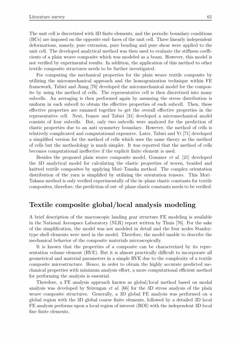
Literature survey 61
The unit cell is discretized with 3D finite elements, and the periodic boundary conditions(BCs) are imposed on the opposite end–faces of the unit cell. Three linearly independentdeformations, namely, pure extension, pure bending and pure shear were applied to theunit cell. The developed analytical method was then used to evaluate the stiffness coeffi-cients of a plain weave composite which was modeled as a beam. However, this model isnot verified by experimental results. In addition, the application of this method to othertextile composite structures needs to be further investigated.
For computing the mechanical properties for the plain weave textile composite byutilizing the micromechanical approach and the homogenization technique within FEframework, Tabiei and Jiang [70] developed the micromechanical model for the compos-ite by using the method of cells. The representative cell is then discretized into manysubcells. An averaging is then performed again by assuming the stress distribution isuniform in each subcell to obtain the effective properties of each subcell. Then, theseeffective properties are summed together to get the overall effective properties in therepresentative cell. Next, Ivanov and Tabiei [31] developed a micromechanical modelconsists of four subcells. But, only two subcells were analyzed for the prediction ofelastic properties due to an anti–symmetry boundary. However, the method of cells isrelatively complicated and computational expensive. Later, Tabiei and Yi [71] developeda simplified version for the method of cells which uses the same theory as the methodof cells but the methodology is much simpler. It was reported that the method of cellsbecomes computational ineffective if the explicit finite element is used.
Besides the proposed plain weave composite model, Gommer et al. [21] developedthe 3D analytical model for calculating the elastic properties of woven, braided andknitted textile composites by applying Mori–Tanaka method. The complex orientationdistribution of the yarn is simplified by utilizing the orientation tensors. This Mori–Takana method is only verified experimentally of the in–plane elastic constants for textilecomposites, therefore, the prediction of out–of–plane elastic constants needs to be verified.
Textile composite global/local analysis modeling
A brief description of the macroscopic landing gear structure FE modeling is availablein the National Aerospace Laboratory (NLR) report written by Thuis [76]. For the sakeof the simplification, the model was not modeled in detail and the four nodes Stanley-type shell elements were used in the model. Therefore, the model unable to describe themechanical behavior of the composite materials microscopically.
It is known that the properties of a composite can be characterized by its repre-sentation volume element (RVE). But it is almost practically difficult to incorporate allgeometrical and material parameters in a simple RVE due to the complexity of a textilecomposite microstructure. Hence, in order to obtain the highly accurate predicted me-chanical properties with minimum analysis effort, a more computational efficient methodfor performing the analysis is essential.
Therefore, a FE analysis approach known as global/local method based on modalanalysis was developed by Srirengan et al. [66] for the 3D stress analysis of the plainweave composite structures. Generally, a 3D global FE analysis was performed on aglobal region with the 3D global coarse finite elements, followed by a detailed 3D localFE analysis performs upon a local region of interest (ROI) with the independent 3D localfine finite elements.
62 Appendix A
Whitcomb [85] developed an iterative global/local FE analysis method. The basicidea of this method was that the displacements or stresses on a global model with coarsemesh can be obtained with an appropriate impose of the boundary conditions on theglobal/local interfaces in a refined local model. However, it was reported that there wasa potential problem due to the differences in stiffness on the global/local boundaries.
Later, Whitcomb et al. [86] proposed a global/local stress analysis procedure whichused homogenized engineering material properties to accelerate the global stress analysisfor the textile composites. The homogenized engineering properties is used owing to therelatively large size of a unit cell for the textile composite compared with the unidirec-tional laminated composites. However, this method was validated only in 2D problem,thus, an application of this method in 3D problem needs to be further investigated. Itwas reported that the accuracy of the calculated stress was poor for exterior unit cells ina global model due to the free boundary effects.
Takano et al. [72] named the global/local modeling as hierarchical modeling for thetextile composites because four–level hierarchy is considered from both material andstructural point of views. The hierarchy of structure consists of global and local levels,whereas, the hierarchy of material consists of meso and micro levels. From the viewpointof heterogeneous material, a unit cell model of the textile composites consists of yarns(fiber bundles) and matrix which is considered as a mesoscale model. In microscalemodel, the yarns are modeled as a medium composed of mono–filament and matrix. In allhierarchical levels, the homogenization analysis method is used for obtaining the relativelygood accuracy results. It was claimed that remarkable inexpensive computational effortin terms of central processing unit (CPU) time and memory especially finite elementgeneration can be achieved in this hierarchical context.
Multi–scale homogenization approach
For the past decades, vast amount of multi–scale modeling techniques for heteroge-neous materials were proposed, such as analytical homogenization (Suquet [69]), asymp-totic homogenization (Yi et al. [91], Chung et al. [8]), variational multi–scale methods(Miehe [47]) and computational homogenization (Kouznetsova et al. [38, 39], Miehe et
al. [50], Miehe [48], Mouline and Suquet [52], Miehe and Koch [49], Michel et al. [46],Feyel and Chaboche [13], Terada et al. [74]). Among these homogenization techniques,the computational homogenization (also known as FE2 method [13]) is probably one ofthe most accurate techniques [17]. It depends on the nested solution algorithm for amacrostructure at the microstructure boundary value problem. Therefore, it providesan accurate multi–scale solution to many engineering materials with heterogeneous char-acteristic, such as metal alloy systems, porous media, polycrystalline materials [16, 37].Hence, it is reasonable to believe that the computational homogenization framework hasthe capability to solve the relatively complex textile composites problems by bridging itsmacro–scale and micro–scale.
However, the multi–scale computational homogenization method is not better or worsethan the widely used global/local method in the textile composites analysis. The selectionbetween both methods should base on the descriptions of a specific engineering problem.The global/local method is no more than a FE analysis through the mesh refinementtechnique on a region of interest (ROI), e.g. crack tips or specific regions with highstresses or strains. Whereas, the multi–scale computational homogenization approach

Literature survey 63
is used optimally for predicting the collective multi–phase response of a microstructurecollectively. Moreover, the multi-scale computational homogenization approach enablesto provide the detailed microstructural phenomenon at each macroscopic region. As aresult, the contribution of the mechanical mechanicsms from micro–level to macro–levelcan be studied in detailed.
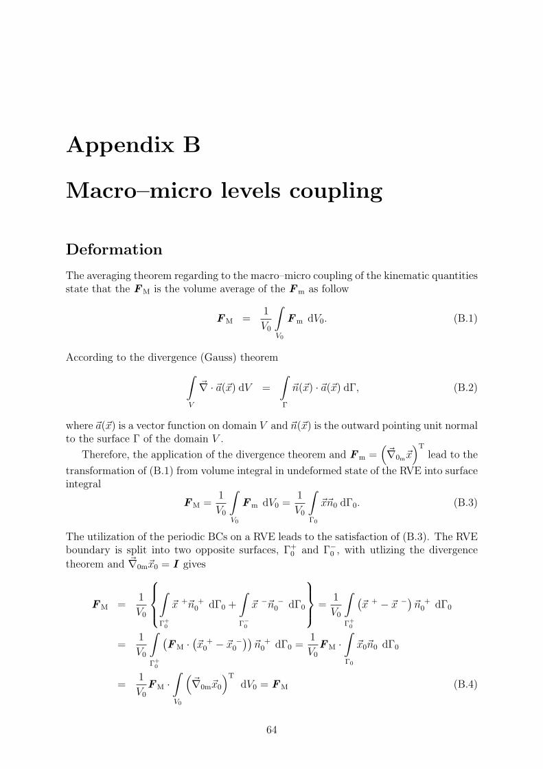
Appendix B
Macro–micro levels coupling
Deformation
The averaging theorem regarding to the macro–micro coupling of the kinematic quantitiesstate that the FM is the volume average of the Fm as follow
FM =1
V0
∫
V0
Fm dV0. (B.1)
According to the divergence (Gauss) theorem
∫
V
~∇ · ~a(~x) dV =
∫
Γ
~n(~x) · ~a(~x) dΓ, (B.2)
where ~a(~x) is a vector function on domain V and ~n(~x) is the outward pointing unit normalto the surface Γ of the domain V .
Therefore, the application of the divergence theorem and Fm =(~∇0m~x
)Tlead to the
transformation of (B.1) from volume integral in undeformed state of the RVE into surfaceintegral
FM =1
V0
∫
V0
Fm dV0 =1
V0
∫
Γ0
~x~n0 dΓ0. (B.3)
The utilization of the periodic BCs on a RVE leads to the satisfaction of (B.3). The RVEboundary is split into two opposite surfaces, Γ+
0 and Γ−
0 , with utlizing the divergence
theorem and ~∇0m~x0 = I gives
FM =1
V0
∫
Γ+0
~x +~n +0 dΓ0 +
∫
Γ−
0
~x −~n −
0 dΓ0
=1
V0
∫
Γ+0
(~x + − ~x −
)~n +0 dΓ0
=1
V0
∫
Γ+0
(FM ·
(~x +0 − ~x −
0
))~n +0 dΓ0 =
1
V0
FM ·
∫
Γ0
~x0~n0 dΓ0
=1
V0
FM ·
∫
V0
(~∇0m~x0
)TdV0 = FM (B.4)
64
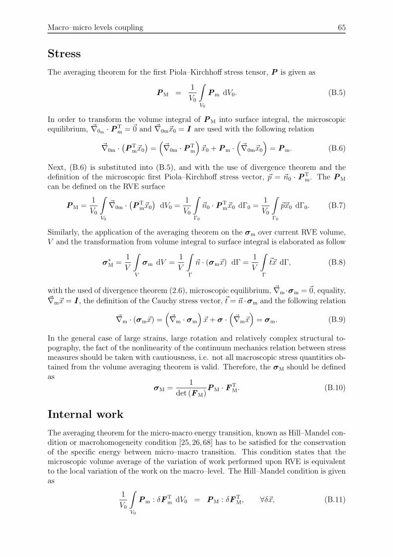
Macro–micro levels coupling 65
Stress
The averaging theorem for the first Piola–Kirchhoff stress tensor, P is given as
PM =1
V0
∫
V0
Pm dV0. (B.5)
In order to transform the volume integral of PM into surface integral, the microscopicequilibrium, ~∇0m ·PT
m = ~0 and ~∇0m~x0 = I are used with the following relation
~∇0m ·(P
Tm~x0
)=(~∇0m ·PT
m
)~x0 +Pm ·
(~∇0m~x0
)= Pm. (B.6)
Next, (B.6) is substituted into (B.5), and with the use of divergence theorem and thedefinition of the microscopic first Piola–Kirchhoff stress vector, ~p = ~n0 · P
Tm. The PM
can be defined on the RVE surface
PM =1
V0
∫
V0
~∇0m ·(P
Tm~x0
)dV0 =
1
V0
∫
Γ0
~n0 ·PTm~x0 dΓ0 =
1
V0
∫
Γ0
~p~x0 dΓ0. (B.7)
Similarly, the application of the averaging theorem on the σm over current RVE volume,V and the transformation from volume integral to surface integral is elaborated as follow
σ∗
M =1
V
∫
V
σm dV =1
V
∫
Γ
~n · (σm~x) dΓ =1
V
∫
Γ
~t~x dΓ, (B.8)
with the used of divergence theorem (2.6), microscopic equilibrium, ~∇m ·σm = ~0, equality,~∇m~x = I , the definition of the Cauchy stress vector, ~t = ~n ·σm and the following relation
~∇m · (σm~x) =(~∇m · σm
)~x+ σ ·
(~∇m~x
)= σm. (B.9)
In the general case of large strains, large rotation and relatively complex structural to-pography, the fact of the nonlinearity of the continuum mechanics relation between stressmeasures should be taken with cautiousness, i.e. not all macroscopic stress quantities ob-tained from the volume averaging theorem is valid. Therefore, the σM should be definedas
σM =1
det (FM)PM · FT
M. (B.10)
Internal work
The averaging theorem for the micro-macro energy transition, known as Hill–Mandel con-dition or macrohomogeneity condition [25,26,68] has to be satisfied for the conservationof the specific energy between micro–macro transition. This condition states that themicroscopic volume average of the variation of work performed upon RVE is equivalentto the local variation of the work on the macro–level. The Hill–Mandel condition is givenas
1
V0
∫
V0
Pm : δFTm dV0 = PM : δFT
M, ∀δ~x, (B.11)
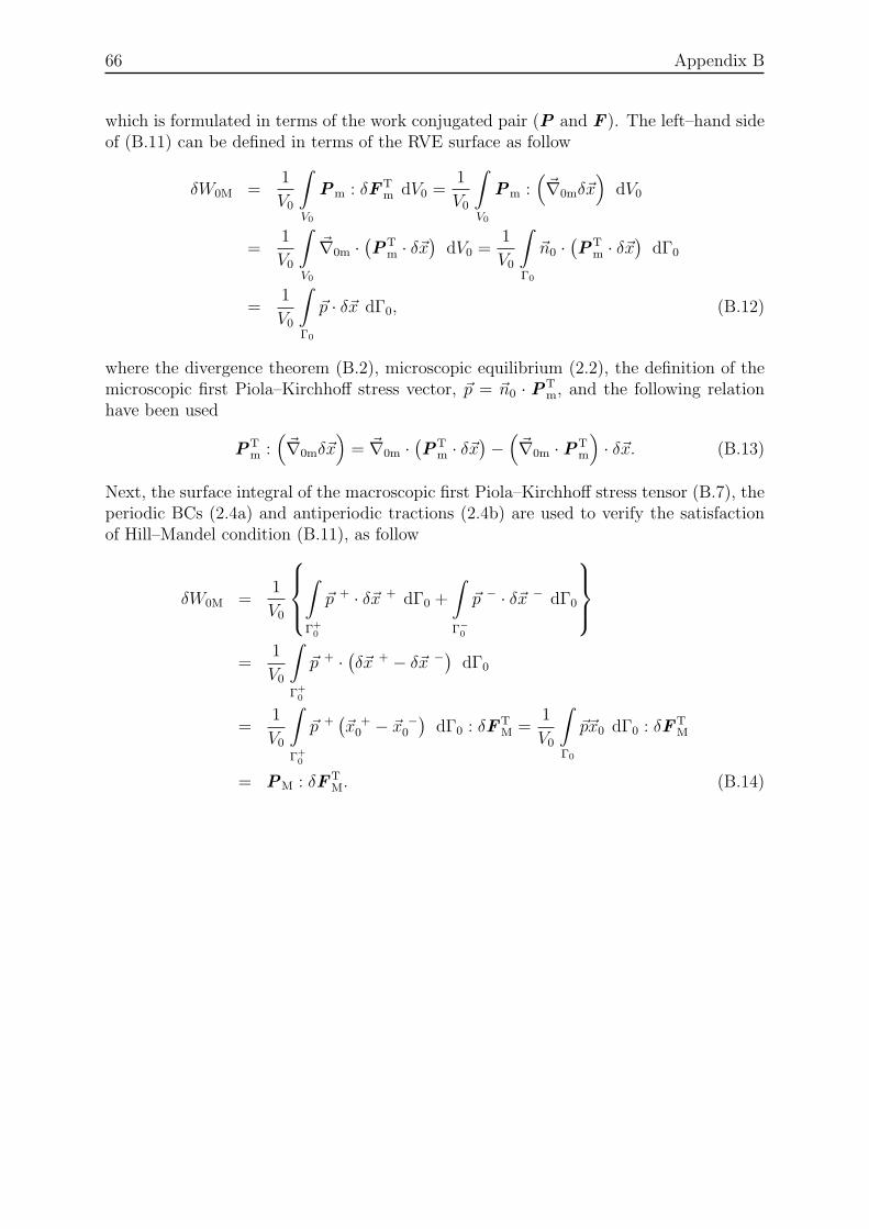
66 Appendix B
which is formulated in terms of the work conjugated pair (P and F ). The left–hand sideof (B.11) can be defined in terms of the RVE surface as follow
δW0M =1
V0
∫
V0
Pm : δFTm dV0 =
1
V0
∫
V0
Pm :(~∇0mδ~x
)dV0
=1
V0
∫
V0
~∇0m ·(P
Tm · δ~x
)dV0 =
1
V0
∫
Γ0
~n0 ·(P
Tm · δ~x
)dΓ0
=1
V0
∫
Γ0
~p · δ~x dΓ0, (B.12)
where the divergence theorem (B.2), microscopic equilibrium (2.2), the definition of themicroscopic first Piola–Kirchhoff stress vector, ~p = ~n0 · P
Tm, and the following relation
have been used
PTm :(~∇0mδ~x
)= ~∇0m ·
(P
Tm · δ~x
)−(~∇0m ·PT
m
)· δ~x. (B.13)
Next, the surface integral of the macroscopic first Piola–Kirchhoff stress tensor (B.7), theperiodic BCs (2.4a) and antiperiodic tractions (2.4b) are used to verify the satisfactionof Hill–Mandel condition (B.11), as follow
δW0M =1
V0
∫
Γ+0
~p + · δ~x + dΓ0 +
∫
Γ−
0
~p − · δ~x − dΓ0
=1
V0
∫
Γ+0
~p + ·(δ~x + − δ~x −
)dΓ0
=1
V0
∫
Γ+0
~p +(~x +0 − ~x −
0
)dΓ0 : δF
TM =
1
V0
∫
Γ0
~p~x0 dΓ0 : δFTM
= PM : δFTM. (B.14)
Appendix C
Microscopic level boundary valueproblem
The RVE boundary value problem imposed with the periodic BCs can be solved numer-ically with FE method. Following the FE method, the weak formulation procedure andFE discretization are performed on the equilibrium equation (2.2) with account for theconstitutive relation (2.3) lead to a non–linear algebraic equations system
f˜internal
(u˜)= f˜external, (C.1)
expressing the equilibrium in external forces, f˜external and internal forces, f
˜internal in terms
of unknown nodal displacements, u˜. This system can be solved through imposing the
BCs. Therefore, the periodic BCs (2.4a) have to be rewritten into an appropriate formatfor its application in the FE framework. Consider a 3D periodic RVE schematicallydepicted in Figure 2.5. It is assumed that the FE discretization is performed such that thecorresponding opposite surfaces of the RVE is discretized into an equivalent distributionof nodes. And, the surfaces of the RVE can be split into top, bottom, left, right, frontand back surfaces. Due to the initial periodicity of the RVE, the respective pair of nodeson the top–bottom, right–left, and front–back surfaces in the undeformed state (or initialconfiguration) can be written as
~x0top − ~x0bottom = ~x05 − ~x01 , (C.2a)
~x0right − ~x0left = ~x02 − ~x01 , (C.2b)
~x0front − ~x0back = ~x01 − ~x04 , (C.2c)
where ~x0p is the initial position vector of the prescribed four corner nodes (also knownas control nodes, master nodes [11] or control vertices [78]), p (p = 1, 2, 4, 5), as shown inFigure 2.4. The ~x0right and ~x0left , ~x0front and ~x0back , ~x0top and ~x0bottom are the initial positionvectors for the respective pair of nodes on the right and left, front and back, top andbottom surfaces of the RVE, respectively. According to (2.4a), by considering the pairs ofrespective nodes on the opposite surfaces, the periodic BCs in deformed state (or currentconfiguration) can be written as
~xtop − ~xbottom = FM · (~x05 − ~x01) = ~x5 − ~x1, (C.3a)
~xright − ~xleft = FM · (~x02 − ~x01) = ~x2 − ~x1, (C.3b)
~xfront − ~xback = FM · (~x01 − ~x04) = ~x1 − ~x4. (C.3c)
67
68 Appendix C
where the relation of the position vectors for the four corner nodes between deformedand undeformed states as shown below has been used in (C.3)
~xp = FM · ~x0p . p = 1, 2, 4, 5 (C.4)
Then, the periodic BCs in deformed state can be rewritten as
~xtop = ~xbottom + ~x5 − ~x1, (C.5a)
~xright = ~xleft + ~x2 − ~x1, (C.5b)
~xfront = ~xback + ~x1 − ~x4. (C.5c)
Besides prescribing the position vectors for every respective pair of nodes, they can beformulated in terms of displacements, ~u
~utop = ~ubottom + ~u5 − ~u1, (C.6a)
~uright = ~uleft + ~u2 − ~u1, (C.6b)
~ufront = ~uback + ~u1 − ~u4. (C.6c)
The relation of ~u with ~x0 can be expressed as
~up = (FM − I ) · ~x0p , p = 1, 2, 4, 5, (C.7)
where I is the identity tensor.Next, the (C.6) can be discretized and partitioned into a set of homogeneous con-
straints in matrix format
[C i Cd]
[u˜iu˜d
]= 0˜, (C.8)
where C is the matrix containing the coefficients in the constraint relations and u˜is the
column with the degrees of freedom (DOF) involved in the constraints. The subscripts“i” and “d” are denoted as independent and dependent for the respective parameter,respectively. In the following, the procedure of eliminating of the dependent DOF fromthe system of equations is used, i.e. the u
˜ihas to be retained in the system and u
˜dhas to
be eliminated from the system. Due to the equivalent total number of dependent DOF,u˜d
as total number of constraint equations in (C.8). Thus, the matrix, Cd is square andnon-singular. The solution for u
˜dyields
u˜d
= Cdi u˜i, with Cdi = −C−1
d C i. (C.9)
Then, the column u˜in (C.8) may be further rewritten into
[u˜iu˜d
]= T u
˜i, with T =
[I
Cdi
], (C.10)
where I is a unit matrix of size [Ni ×Ni], with Ni is the number of the independent DOF.The non–linear system of equations (C.1) is linearized to a linear system in the it-
erative corrections, δu˜
to the current estimation, u˜. This linearized system may be
partitioned as
[Kii Kid
Kdi Kdd
] [δu˜iδu˜d
]=
[~f˜iexternal
− ~f˜iinternal~f
˜dexternal− ~f˜dinternal
]=
[δr˜iδr˜d
], (C.11)

Microscopic level boundary value problem 69
with the residual nodal forces, δr˜at the right–hand side. The constraint equations in
(C.11) are linear. Thus, their linearization is straightforward and the application of the(C.10) to the system (C.11) gives
[I CT
di
] [ Kii Kid
Kdi Kdd
] [I
Cdi
]δu˜i
=[I CT
di
] [ δr˜iδr˜d
], (C.12)
after rewritten the (C.12) gives
[Kii +KdiCdi + CT
diKdi + CTdiKddCdi
]δu˜i
=[δr˜i
+ CTdiδr˜d
]. (C.13)
The column u˜i
in (C.13) includes the displacement of the prescribed corner nodes, u˜p.
Therefore, the boundary conditions (C.7) can be applied to the system (C.13).
Appendix D
Macroscopic stress calculation
The RVE volume averaged stress has to be extracted after analyzing the RVE. Of course,the PM can be computed numerically through the volume integral (2.8). However, it iscomputationally inefficient because the unit cell volume for the textile composites can betypically several orders of magnitude larger than the unit cell volume of the conventionalunidirectional laminated composites [33]. Therefore, it is computationally more efficientto compute the PM through the surface integral [37] which can be further simplified forthe case of the periodic BCs as discussed in this section.
First, consider that all the forces acting on the the RVE surface are subjected to theperiodic BCs (C.6) and (C.7). The reaction (resulting) external forces, ~f e
p are acted atthe four prescribed corner nodes, p (p = 1, 2, 4, 5). In addition, there are forces involvedin every constraint (tying) relation C.6. For instance, each constraint relation of thecorresponding pairs of nodes on the top–bottom surfaces, there are tying forces, ~p t
top,
~p tbottom, ~p
tB1 , and ~p tB
5 at the nodes on the top surface, bottom surface, corner node 1, andcorner node 5, respectively. Similarly, there are tying forces, ~p t
front, ~ptback, ~p
tF1 , and ~p tF
4 forthe front–back constraint relations and the tying forces, ~p t
right, ~ptleft, ~p
tL2 and ~p tL
1 for theright–left constraint relations. All these forces are schematically depicted in Figure D.1.Each constraint satisfied the condition of zero virtual work according to the principle ofvirtual work which implies that tying forces applied to the RVE do no virtual work, thus
~p tbottom · δ~xbottom + ~p t
top · δ~xtop + ~p tB5 · δ~x5 + ~p tB
1 · δ~x1 = 0, (D.1a)
~p tleft · δ~xleft + ~p t
right · δ~xright + ~p tL2 · δ~x2 + ~p tL
1 · δ~x1 = 0, (D.1b)
~p tfront · δ~xfront + ~p t
back · δ~xback + ~p tF4 · δ~x4 + ~p tF
1 · δ~x1 = 0. (D.1c)
Substitution of the variation of the periodic constraint relations (C.5) into (D.1) gives
(~p tbottom + ~p t
top
)· δ~xbottom +
(~p tB1 − ~p t
top
)· δ~x1 +
(~p ttop + ~p tB
5
)· δ~x5 = 0, (D.2a)
(~p tleft + ~p t
right
)· δ~xleft +
(~p tL1 − ~p t
right
)· δ~x1 +
(~p tright + ~p tL
2
)· δ~x2 = 0, (D.2b)
(~p tfront + ~p t
back
)· δ~xback +
(~p tF1 + ~p t
front
)· δ~x1 +
(~p tF4 − ~p t
front
)· δ~x4 = 0. (D.2c)
These relations should hold for any δ~xbottom, δ~xleft, δ~xback, δ~x1, δ~x2, δ~x4, δ~x5. Thus, therelation between tying forces are
~p tbottom = −~p t
top = −~p tB1 = ~p tB
5 , (D.3a)
~p tleft = −~p t
right = −~p tL1 = ~p tL
2 , (D.3b)
~p tfront = −~p t
back = −~p tF1 = ~p tF
4 . (D.3c)
70
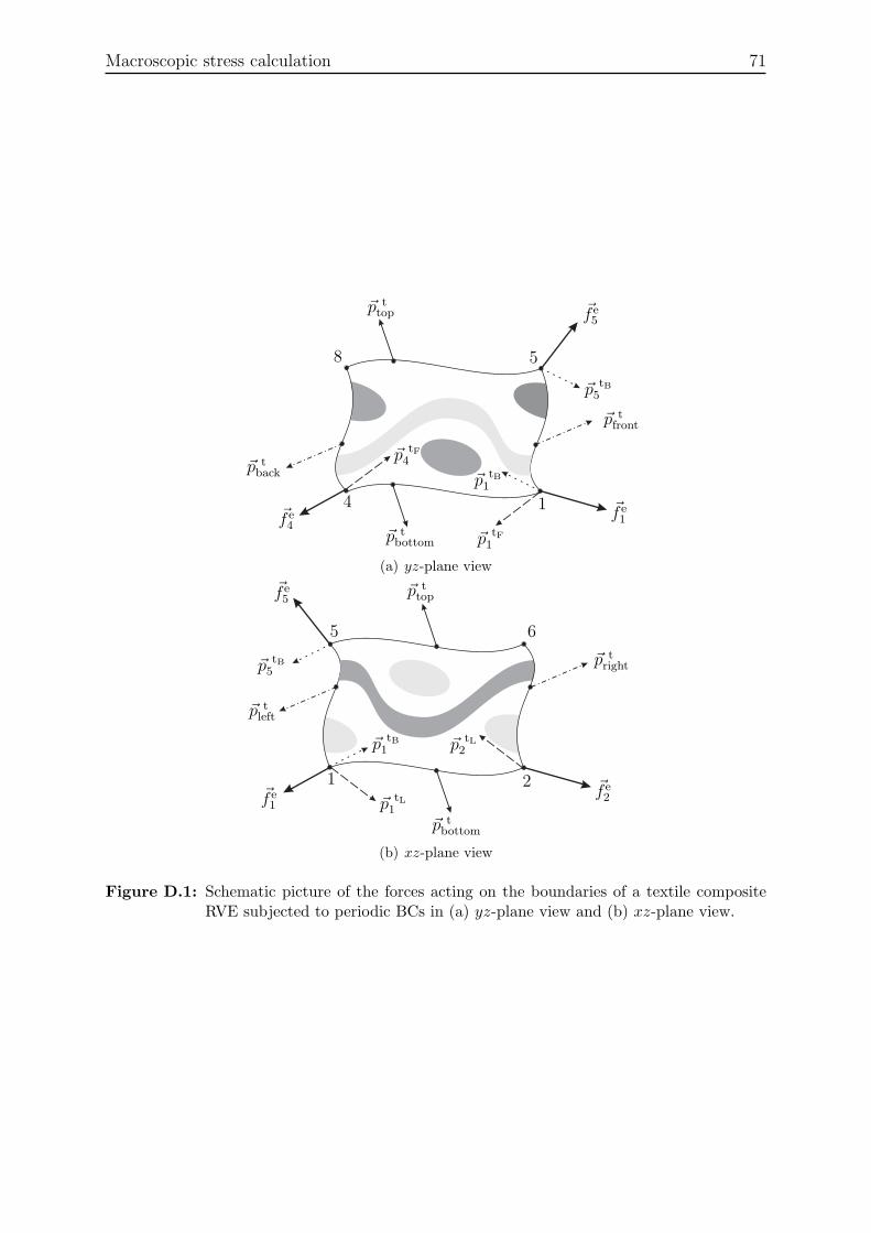
Macroscopic stress calculation 71
4 1
58
~f e4
~f e1
~f e5
~p ttop
~p tbottom
~p tfront
~p tback
~p tF1
~p tF4
~p tB1
~p tB5
(a) yz-plane view
1 2
65
~f e1
~f e2
~f e5
~p ttop
~p tbottom
~p tright
~p tleft
~p tL2
~p tL1
~p tB1
~p tB5
(b) xz-plane view
Figure D.1: Schematic picture of the forces acting on the boundaries of a textile compositeRVE subjected to periodic BCs in (a) yz-plane view and (b) xz-plane view.
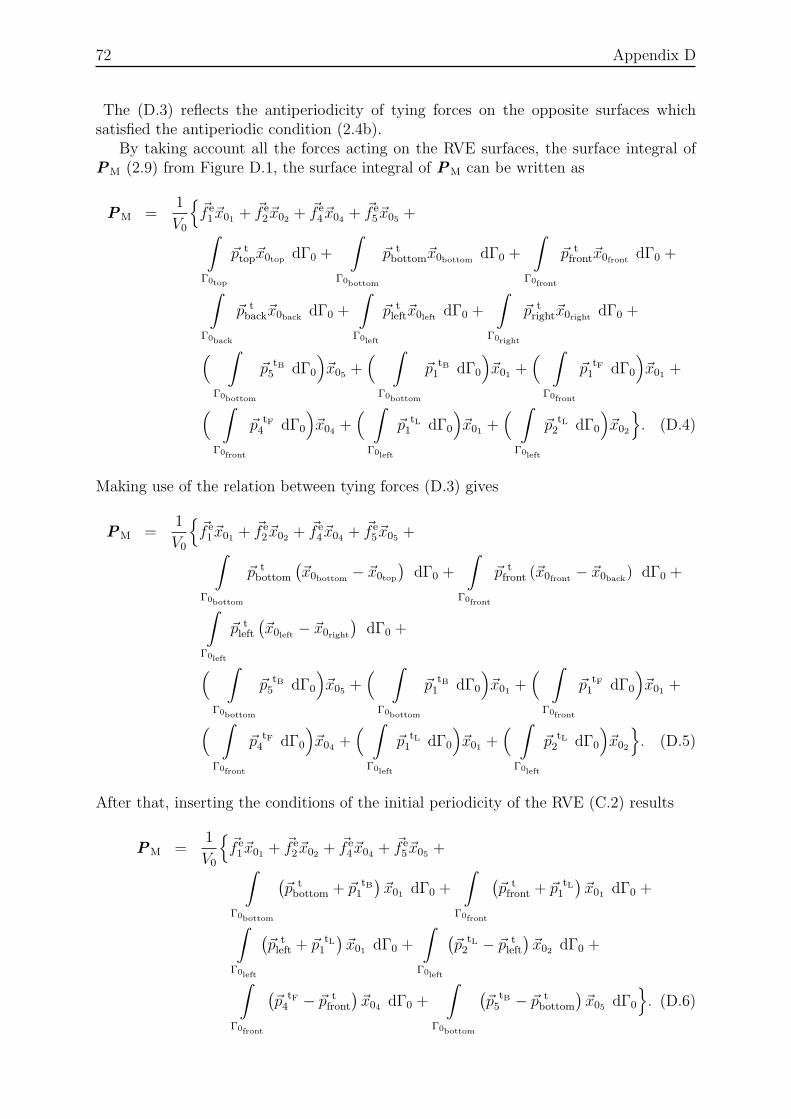
72 Appendix D
The (D.3) reflects the antiperiodicity of tying forces on the opposite surfaces whichsatisfied the antiperiodic condition (2.4b).
By taking account all the forces acting on the RVE surfaces, the surface integral ofPM (2.9) from Figure D.1, the surface integral of PM can be written as
PM =1
V0
{~f e1~x01 +
~f e2~x02 +
~f e4~x04 +
~f e5~x05 +
∫
Γ0top
~p ttop~x0top dΓ0 +
∫
Γ0bottom
~p tbottom~x0bottom dΓ0 +
∫
Γ0front
~p tfront~x0front dΓ0 +
∫
Γ0back
~p tback~x0back dΓ0 +
∫
Γ0left
~p tleft~x0left dΓ0 +
∫
Γ0right
~p tright~x0right dΓ0 +
( ∫
Γ0bottom
~p tB5 dΓ0
)~x05 +
( ∫
Γ0bottom
~p tB1 dΓ0
)~x01 +
( ∫
Γ0front
~p tF1 dΓ0
)~x01 +
( ∫
Γ0front
~p tF4 dΓ0
)~x04 +
( ∫
Γ0left
~p tL1 dΓ0
)~x01 +
( ∫
Γ0left
~p tL2 dΓ0
)~x02
}. (D.4)
Making use of the relation between tying forces (D.3) gives
PM =1
V0
{~f e1~x01 +
~f e2~x02 +
~f e4~x04 +
~f e5~x05 +
∫
Γ0bottom
~p tbottom
(~x0bottom − ~x0top
)dΓ0 +
∫
Γ0front
~p tfront (~x0front − ~x0back) dΓ0 +
∫
Γ0left
~p tleft
(~x0left − ~x0right
)dΓ0 +
( ∫
Γ0bottom
~p tB5 dΓ0
)~x05 +
( ∫
Γ0bottom
~p tB1 dΓ0
)~x01 +
( ∫
Γ0front
~p tF1 dΓ0
)~x01 +
( ∫
Γ0front
~p tF4 dΓ0
)~x04 +
( ∫
Γ0left
~p tL1 dΓ0
)~x01 +
( ∫
Γ0left
~p tL2 dΓ0
)~x02
}. (D.5)
After that, inserting the conditions of the initial periodicity of the RVE (C.2) results
PM =1
V0
{~f e1~x01 +
~f e2~x02 +
~f e4~x04 +
~f e5~x05 +
∫
Γ0bottom
(~p tbottom + ~p tB
1
)~x01 dΓ0 +
∫
Γ0front
(~p tfront + ~p tL
1
)~x01 dΓ0 +
∫
Γ0left
(~p tleft + ~p tL
1
)~x01 dΓ0 +
∫
Γ0left
(~p tL2 − ~p t
left
)~x02 dΓ0 +
∫
Γ0front
(~p tF4 − ~p t
front
)~x04 dΓ0 +
∫
Γ0bottom
(~p tB5 − ~p t
bottom
)~x05 dΓ0
}. (D.6)
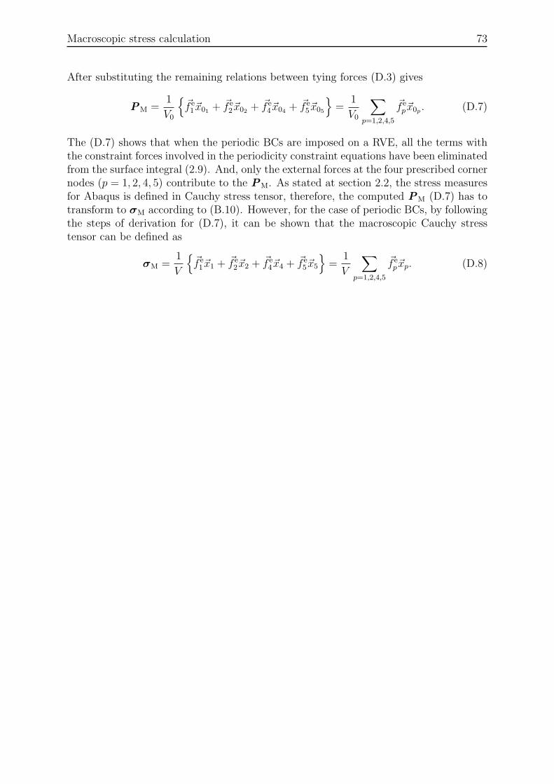
Macroscopic stress calculation 73
After substituting the remaining relations between tying forces (D.3) gives
PM =1
V0
{~f e1~x01 +
~f e2~x02 +
~f e4~x04 +
~f e5~x05
}=
1
V0
∑
p=1,2,4,5
~f ep~x0p . (D.7)
The (D.7) shows that when the periodic BCs are imposed on a RVE, all the terms withthe constraint forces involved in the periodicity constraint equations have been eliminatedfrom the surface integral (2.9). And, only the external forces at the four prescribed cornernodes (p = 1, 2, 4, 5) contribute to the PM. As stated at section 2.2, the stress measuresfor Abaqus is defined in Cauchy stress tensor, therefore, the computed PM (D.7) has totransform to σM according to (B.10). However, for the case of periodic BCs, by followingthe steps of derivation for (D.7), it can be shown that the macroscopic Cauchy stresstensor can be defined as
σM =1
V
{~f e1~x1 + ~f e
2~x2 + ~f e4~x4 + ~f e
5~x5
}=
1
V
∑
p=1,2,4,5
~f ep~xp. (D.8)
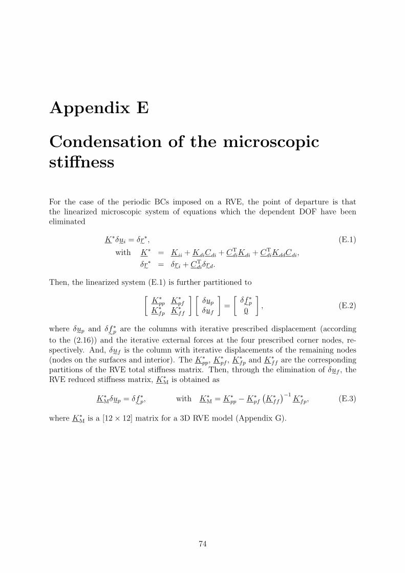
Appendix E
Condensation of the microscopicstiffness
For the case of the periodic BCs imposed on a RVE, the point of departure is thatthe linearized microscopic system of equations which the dependent DOF have beeneliminated
K∗δu˜i
= δr˜∗, (E.1)
with K∗ = Kii +KdiCdi + CTdiKdi + CT
diKddCdi,
δr˜∗ = δr
˜i+ CT
diδr˜d.
Then, the linearized system (E.1) is further partitioned to
[K∗
pp K∗
pf
K∗
fp K∗
ff
] [δu˜pδu˜f
]=
[δf˜∗
p
0˜
], (E.2)
where δu˜p
and δf˜∗
p are the columns with iterative prescribed displacement (according
to the (2.16)) and the iterative external forces at the four prescribed corner nodes, re-spectively. And, δu
˜fis the column with iterative displacements of the remaining nodes
(nodes on the surfaces and interior). The K∗
pp, K∗
pf , K∗
fp and K∗
ff are the correspondingpartitions of the RVE total stiffness matrix. Then, through the elimination of δu
˜f, the
RVE reduced stiffness matrix, K∗
M is obtained as
K∗
Mδu˜p= δf˜∗
p, with K∗
M = K∗
pp −K∗
pf
(K∗
ff
)−1
K∗
fp, (E.3)
where K∗
M is a [12× 12] matrix for a 3D RVE model (Appendix G).
74
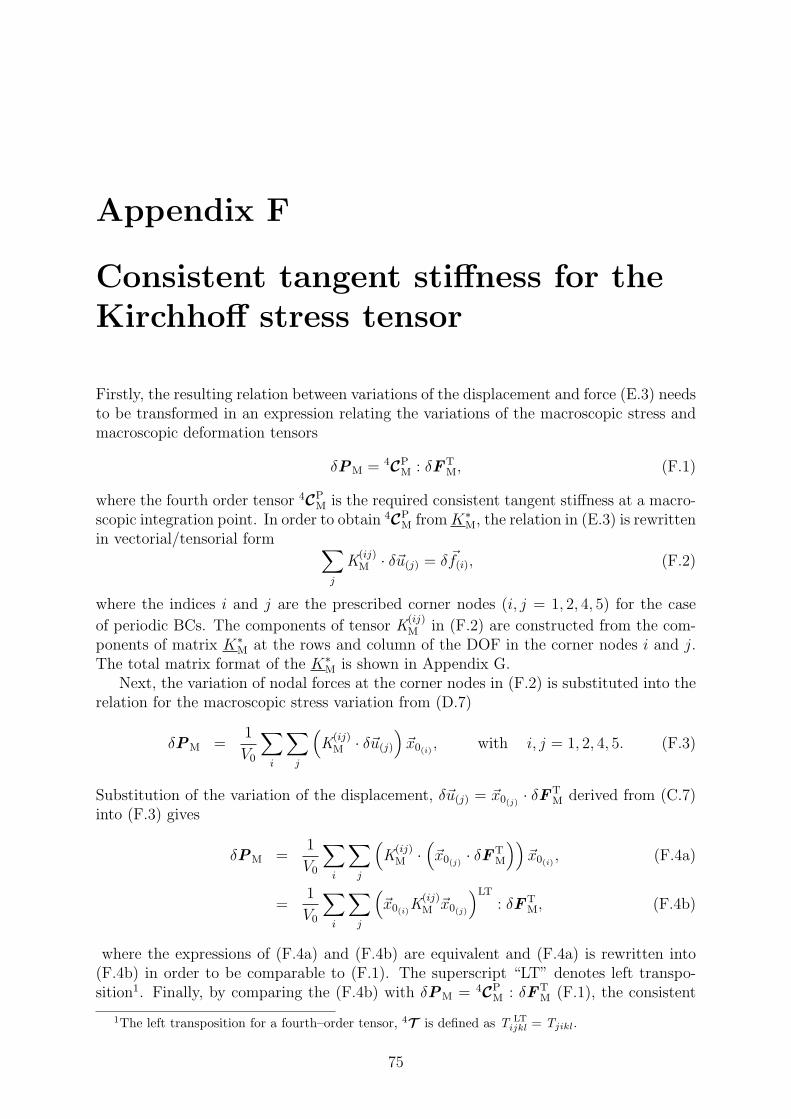
Appendix F
Consistent tangent stiffness for theKirchhoff stress tensor
Firstly, the resulting relation between variations of the displacement and force (E.3) needsto be transformed in an expression relating the variations of the macroscopic stress andmacroscopic deformation tensors
δPM = 4CPM : δFT
M, (F.1)
where the fourth order tensor 4CPM is the required consistent tangent stiffness at a macro-
scopic integration point. In order to obtain 4CPM fromK∗
M, the relation in (E.3) is rewrittenin vectorial/tensorial form ∑
j
K(ij)M · δ~u(j) = δ ~f(i), (F.2)
where the indices i and j are the prescribed corner nodes (i, j = 1, 2, 4, 5) for the case
of periodic BCs. The components of tensor K(ij)M in (F.2) are constructed from the com-
ponents of matrix K∗
M at the rows and column of the DOF in the corner nodes i and j.The total matrix format of the K∗
M is shown in Appendix G.Next, the variation of nodal forces at the corner nodes in (F.2) is substituted into the
relation for the macroscopic stress variation from (D.7)
δPM =1
V0
∑
i
∑
j
(K
(ij)M · δ~u(j)
)~x0(i) , with i, j = 1, 2, 4, 5. (F.3)
Substitution of the variation of the displacement, δ~u(j) = ~x0(j) · δFTM derived from (C.7)
into (F.3) gives
δPM =1
V0
∑
i
∑
j
(K
(ij)M ·
(~x0(j) · δF
TM
))~x0(i) , (F.4a)
=1
V0
∑
i
∑
j
(~x0(i)K
(ij)M ~x0(j)
)LT: δFT
M, (F.4b)
where the expressions of (F.4a) and (F.4b) are equivalent and (F.4a) is rewritten into(F.4b) in order to be comparable to (F.1). The superscript “LT” denotes left transpo-sition1. Finally, by comparing the (F.4b) with δPM = 4C
PM : δFT
M (F.1), the consistent
1The left transposition for a fourth–order tensor, 4T is defined as T LT
ijkl = Tjikl.
75
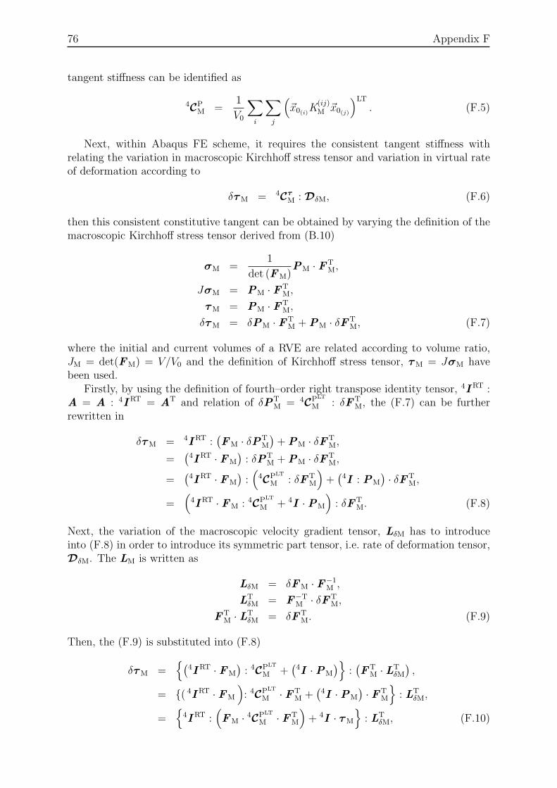
76 Appendix F
tangent stiffness can be identified as
4CPM =
1
V0
∑
i
∑
j
(~x0(i)K
(ij)M ~x0(j)
)LT. (F.5)
Next, within Abaqus FE scheme, it requires the consistent tangent stiffness withrelating the variation in macroscopic Kirchhoff stress tensor and variation in virtual rateof deformation according to
δτM = 4Cτ
M : DδM, (F.6)
then this consistent constitutive tangent can be obtained by varying the definition of themacroscopic Kirchhoff stress tensor derived from (B.10)
σM =1
det (FM)PM · FT
M,
JσM = PM · FTM,
τM = PM · FTM,
δτM = δPM · FTM +PM · δFT
M, (F.7)
where the initial and current volumes of a RVE are related according to volume ratio,JM = det(FM) = V/V0 and the definition of Kirchhoff stress tensor, τM = JσM havebeen used.
Firstly, by using the definition of fourth–order right transpose identity tensor, 4IRT :
A = A : 4IRT = A
T and relation of δPTM = 4C
PLT
M : δFTM, the (F.7) can be further
rewritten in
δτM = 4IRT :
(FM · δPT
M
)+PM · δFT
M,
=(4IRT · FM
): δPT
M +PM · δFTM,
=(4IRT · FM
):(4CPLT
M : δFTM
)+(4I : PM
)· δFT
M,
=(4IRT · FM : 4
CPLT
M + 4I ·PM
): δFT
M. (F.8)
Next, the variation of the macroscopic velocity gradient tensor, LδM has to introduceinto (F.8) in order to introduce its symmetric part tensor, i.e. rate of deformation tensor,DδM. The LM is written as
LδM = δFM · F−1M ,
LTδM = F
−TM · δFT
M,
FTM · LT
δM = δFTM. (F.9)
Then, the (F.9) is substituted into (F.8)
δτM ={(
4IRT · FM
): 4CPLT
M +(4I ·PM
)}:(F
TM · LT
δM
),
= {( 4IRT · FM
): 4CPLT
M · FTM +
(4I ·PM
)· FT
M
}: LT
δM,
={4IRT :
(FM · 4CPLT
M · FTM
)+ 4
I · τM
}: LT
δM, (F.10)
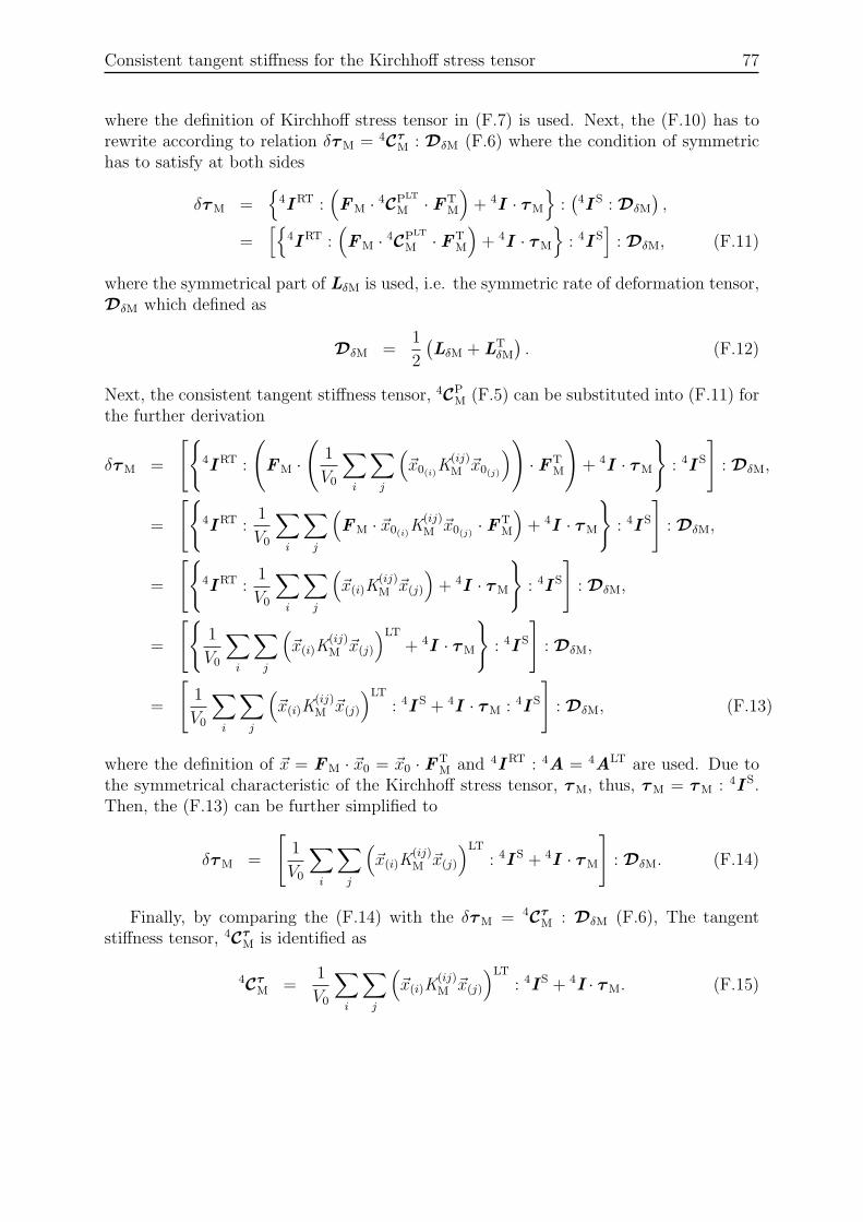
Consistent tangent stiffness for the Kirchhoff stress tensor 77
where the definition of Kirchhoff stress tensor in (F.7) is used. Next, the (F.10) has torewrite according to relation δτM = 4C
τ
M : DδM (F.6) where the condition of symmetrichas to satisfy at both sides
δτM ={4IRT :
(FM · 4CPLT
M · FTM
)+ 4
I · τM
}:(4IS : DδM
),
=[{
4IRT :
(FM · 4CPLT
M · FTM
)+ 4
I · τM
}: 4IS]: DδM, (F.11)
where the symmetrical part of LδM is used, i.e. the symmetric rate of deformation tensor,DδM which defined as
DδM =1
2
(LδM + L
TδM
). (F.12)
Next, the consistent tangent stiffness tensor, 4CPM (F.5) can be substituted into (F.11) for
the further derivation
δτM =
[{4IRT :
(FM ·
(1
V0
∑
i
∑
j
(~x0(i)K
(ij)M ~x0(j)
))· FT
M
)+ 4
I · τM
}: 4IS
]: DδM,
=
[{4IRT :
1
V0
∑
i
∑
j
(FM · ~x0(i)K
(ij)M ~x0(j) · F
TM
)+ 4
I · τM
}: 4IS
]: DδM,
=
[{4IRT :
1
V0
∑
i
∑
j
(~x(i)K
(ij)M ~x(j)
)+ 4
I · τM
}: 4IS
]: DδM,
=
[{1
V0
∑
i
∑
j
(~x(i)K
(ij)M ~x(j)
)LT+ 4
I · τM
}: 4IS
]: DδM,
=
[1
V0
∑
i
∑
j
(~x(i)K
(ij)M ~x(j)
)LT: 4IS + 4
I · τM : 4IS
]: DδM, (F.13)
where the definition of ~x = FM · ~x0 = ~x0 · FTM and 4
IRT : 4
A = 4A
LT are used. Due tothe symmetrical characteristic of the Kirchhoff stress tensor, τM, thus, τM = τM : 4
IS.
Then, the (F.13) can be further simplified to
δτM =
[1
V0
∑
i
∑
j
(~x(i)K
(ij)M ~x(j)
)LT: 4IS + 4
I · τM
]: DδM. (F.14)
Finally, by comparing the (F.14) with the δτM = 4Cτ
M : DδM (F.6), The tangentstiffness tensor, 4C
τ
M is identified as
4Cτ
M =1
V0
∑
i
∑
j
(~x(i)K
(ij)M ~x(j)
)LT: 4IS + 4
I · τM. (F.15)
Appendix G
Total matrix of the reduced stiffnessmatrix
The total matrix K∗
M for a 3D RVE model has the format as shown in (G.1) where thesuperscripts and subscripts in round brackets refer to the nodes and the DOF at thosenodes, respectively. Each submatrix in (G.1) is considered as the representation of a
second–order tensor, K(ij)M , which the indices i and j are the prescribed corner nodes
(i, j = 1, 2, 4, 5) for the case of periodic BCs.
78
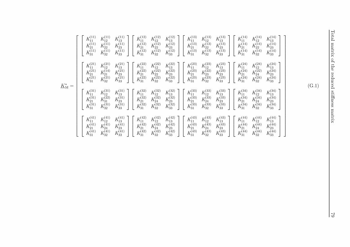
Total
matrix
ofthered
uced
stiffness
matrix
79
K∗
M =
K(11)11 K
(11)12 K
(11)13
K(11)21 K
(11)22 K
(11)23
K(11)31 K
(11)32 K
(11)33
K(12)11 K
(12)12 K
(12)13
K(12)21 K
(12)22 K
(12)23
K(12)31 K
(12)32 K
(12)33
K(13)11 K
(13)12 K
(13)13
K(13)21 K
(13)22 K
(13)23
K(13)31 K
(13)32 K
(13)33
K(14)11 K
(14)12 K
(14)13
K(14)21 K
(14)22 K
(14)23
K(14)31 K
(14)32 K
(14)33
K(21)11 K
(21)12 K
(21)13
K(21)21 K
(14)21 K
(21)23
K(21)31 K
(21)32 K
(21)33
K(22)11 K
(22)12 K
(22)13
K(22)21 K
(22)22 K
(22)23
K(22)31 K
(22)32 K
(22)33
K(23)11 K
(23)12 K
(23)13
K(23)21 K
(22)23 K
(23)23
K(23)31 K
(23)32 K
(23)33
K(24)11 K
(24)12 K
(24)13
K(24)21 K
(22)24 K
(24)23
K(24)31 K
(24)32 K
(24)33
K(31)11 K
(31)12 K
(31)13
K(31)21 K
(22)31 K
(31)23
K(31)31 K
(31)32 K
(31)33
K(32)11 K
(32)12 K
(32)13
K(32)21 K
(32)24 K
(32)23
K(32)31 K
(32)32 K
(32)33
K(33)11 K
(33)12 K
(33)13
K(33)21 K
(33)24 K
(33)23
K(33)31 K
(33)32 K
(33)33
K(34)11 K
(34)12 K
(34)13
K(34)21 K
(34)24 K
(34)23
K(34)31 K
(34)32 K
(34)33
K(41)11 K
(41)12 K
(41)13
K(41)21 K
(41)24 K
(41)23
K(41)31 K
(41)32 K
(41)33
K(42)11 K
(42)12 K
(42)13
K(42)21 K
(42)24 K
(42)23
K(42)31 K
(42)32 K
(42)33
K(43)11 K
(43)12 K
(43)13
K(43)21 K
(43)24 K
(43)23
K(43)31 K
(43)32 K
(43)33
K(44)11 K
(44)12 K
(44)13
K(44)21 K
(44)24 K
(44)23
K(44)31 K
(44)32 K
(44)33
(G.1)
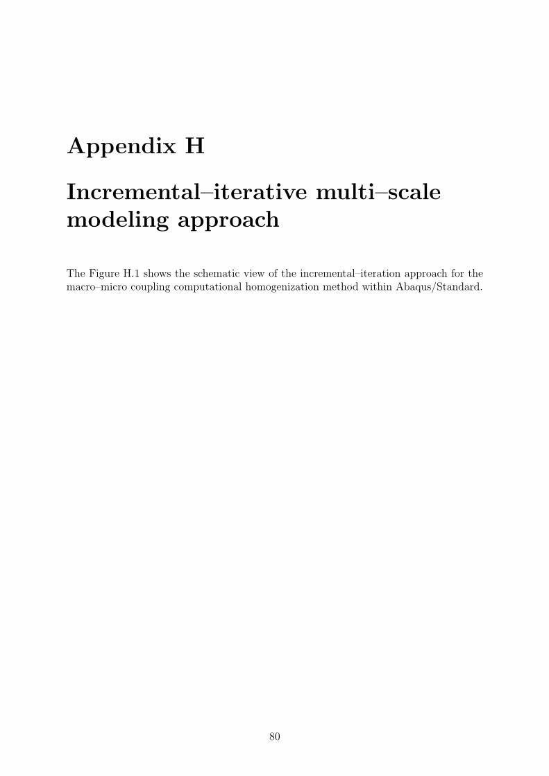
Appendix H
Incremental–iterative multi–scalemodeling approach
The Figure H.1 shows the schematic view of the incremental–iteration approach for themacro–micro coupling computational homogenization method within Abaqus/Standard.
80
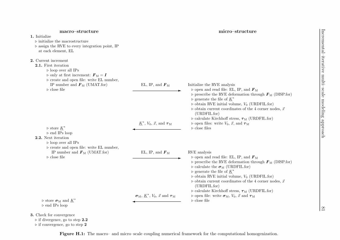
Increm
ental–iterative
multi–scale
modelin
gap
proach
81
macro–structure micro–structure1. Initialize
. initialize the macrostructure
. assign the RVE to every integration point, IPat each element, EL
2. Current increment2.1. First iteration
. loop over all IPs
. only at first increment: FM = I
. create and open file: write EL number,IP number and FM (UMAT.for) EL, IP, and FM Initialize the RVE analysis
. close file - . open and read file: EL, IP, and FM
. prescribe the RVE deformation through FM (DISP.for)
. generate the file of K∗
. obtain RVE initial volume, V0 (URDFIL.for)
. obtain current coordinates of the 4 corner nodes, ~x(URDFIL.for)
. calculate Kirchhoff stress, τM (URDFIL.for)K∗, V0, ~x, and τM . open files: write V0, ~x, and τM
. store K∗
� . close files. end IPs loop
2.2. Next iteration. loop over all IPs. create and open file: write EL number,
IP number and FM (UMAT.for) EL, IP, and FM RVE analysis. close file - . open and read file: EL, IP, and FM
. prescribe the RVE deformation through FM (DISP.for)
. calculate the σM (URDFIL.for)
. generate the file of K∗
. obtain RVE initial volume, V0 (URDFIL.for)
. obtain current coordinates of the 4 corner nodes, ~x(URDFIL.for)
. calculate Kirchhoff stress, τM (URDFIL.for)σM, K∗, V0, ~x and τM . open file: write σM, V0, ~x and τM
. store σM and K∗
� . close file. end IPs loop
3. Check for convergence. if divergence, go to step 2.2
. if convergence, go to step 2
Figure H.1: The macro– and micro–scale coupling numerical framework for the computational homogenization.
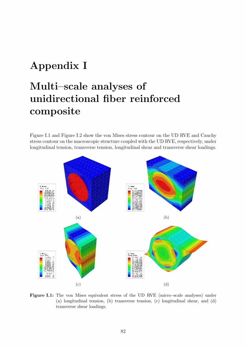
Appendix I
Multi–scale analyses ofunidirectional fiber reinforcedcomposite
Figure I.1 and Figure I.2 show the von Mises stress contour on the UD RVE and Cauchystress contour on the macroscopic structure coupled with the UD RVE, respectively, underlongitudinal tension, transverse tension, longitudinal shear and transverse shear loadings.
(a) (b)
(c) (d)
Figure I.1: The von Mises equivalent stress of the UD RVE (micro–scale analyses) under(a) longitudinal tension, (b) transverse tension, (c) longitudinal shear, and (d)transverse shear loadings.
82
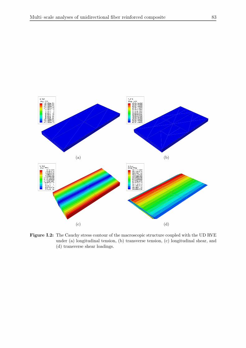
Multi–scale analyses of unidirectional fiber reinforced composite 83
(a) (b)
(c) (d)
Figure I.2: The Cauchy stress contour of the macroscopic structure coupled with the UD RVEunder (a) longitudinal tension, (b) transverse tension, (c) longitudinal shear, and(d) transverse shear loadings.