Embed Size (px)
Citation preview
Chapter 3
Boundary-Value Problems of Potential Theory
The classical boundary-value problems of potential theory corresponding to regular surfaces (such as the sphere, ellipsoid, spheroid, geoid, and Earth's surface) are treated in more detail. Essential tools for establishing Fourier expansions on regular surfaces in terms of trial systems (e.g., single- and multipoles) are the jump and limit relations and their formulation in the L2_ nomenclature. The problems to be addressed here are the exterior Dirichlet problem (EDP), the exterior Neumann problem (ENP) , and the exterior oblique derivative problem (EODP). Moreover, the role of harmonic trial systems (such as outer harmonics, certain kernel representations, etc.) in boundary-value problems corresponding to regular surfaces is described in three different topologies, i.e., the locally uniform, uniform, and Holder topologies.
3.1 Basic Concepts of Potential Theory
First we introduce some settings which are standard in potential theory (see, for example, [134], [160], [198], [219]).
3.1.1 Regular Surfaces
We begin our considerations by introducing the notation of a regular surface: A surface E C 1R3 is called regular (resp. J.l-Holder regular, 0 :s: J.l :s: 1), if it satisfies the following properties:
(i) E divides the three-dimensional Euclidean space 1R3 into the bounded region E int (inner space) and the unbounded region Eext (outer space) defined by Eext = 1R3 \Eint , Eint = Eint U E,
71 W. Freeden et al., Multiscale Potential Theory© Birkhäuser Boston 2004
72 Chapter 3. Boundary-Value Problems of Potential Theory
(ii) 2:int contains the origin,
(iii) 2: is a closed and compact surface free of double points,
(iv) 2: has a continuously differentiable (resp. JL-H6lder continuously differentiable) unit normal field v (more accurately, v~) pointing into the outer space 2:ext .
Geoscientifically regular surfaces 2: are, for example, sphere, ellipsoid, spheroid, geoid, (regular) Earth's surface, etc.
Given a regular surface, then there exist positive constants 0:, (3 such that
0: < O"inf = inf Ixl ~ sup Ixl = O"sup < (3. xE~ xE~
(3.1)
As\usual, Aint , Bint (resp. Aext, Bext ) denote the inner (resp. outer) space of t4e sphere A resp. B around the origin with radius 0: resp. (3. 2:i~L 2:~~f (resp. 2:~~t 2:!~f) denote the inner (resp. outer) space of the sphere 2:inf (~esp. 2:SUP) around the origin with radius O"inf (resp. O"SUP).
The set 2:(T) = {x E JR3 1x = y + TV(Y), Y E 2:} (3.2)
generates a parallel surface which is exterior to 2: for T > 0 and interior for T < O. It is well known from differential geometry (see, e.g., [178]) that if ITI is sufficiently small, then the surface 2:(T) is regular, and the normal to one parallel surface is a normal to the other. According to our regularity assumptions imposed on 2:, the functions
( X y) f-t Iv(x)-v(y)1 (x y) E 2: x 2: x.../.. Y , Ix-yl" , r, ( X y) f-t Iv(x)·(x-y)1 (x y) E 2: x 2: x.../.. Y , Ix-yI2" , r
are bounded. Hence, there exists a constant M > 0 such that
for all (x,y) E 2: x 2:.
LEMMA 3.1
Iv(x) - v(Y)1 ~ Mix - YI, ~v(x)· (x - y)1 ~ Mix - Y1 2 ,
Let 2: be a regular surface. Then
infx,YE~lx + Tvlx) - (y + O"v(y)) I = IT - 0"1
provided that ITI, 10"1 are sufficiently small.
PROOF At first we see that for x, y E 2:
(3.3)
(3.4)
Ix + TV(X) - (y + O"v(Y»12 = I(x - y) + (TV (x) - O"v(Y)W. (3.5)
3.1. Basic Concepts of Potential Theory 73
This leads us to
Ix + TV(V) - (y + av(y)W = Ix - Yl2 + ITv(x) - av(yW (3.6)
+ 2TV(X) . (x - y) - 2av(y) . (x - y).
Furthermore, we obtain
ITv(x) - av(y)12 = T2 + a2 - 2Ta v(x) . v(y) (3.7)
and 1
v(x) . v(y) = 1- "2 lv(x) - v(y)12. (3.8)
In connection with (3.4) (multiplied by -1) we find
where the expression
"1(a, T) = 1 - 2(ITI + lal)M -ITI lalM2 (3.10)
(with ITI, lal sufficiently small) is positive. But this shows us that
Ix + TV(X) - (y + av(y))1 2: IT - al· (3.11)
From the identity
Ix + TV(X) - (x + av(x))1 = IT - al (3.12)
we finally obtain the desired result. I
From [77] we borrow the following lemma.
LEMMA 3.2 Let A (more explicitly, AE) be a continuous unit vector field on ~ forming at any point on ~ with the outside normal v an angle with
infxEE (A(X) . v(x)) > 0. (3.13)
Then there exist constants 8 E (0,00), f3 E (0,1), with
IA(x) . (x - y)1 ~ f3lx - yl (3.14)
for Ix - yl ~ 8.
We continue our considerations with the following estimate.
74 Chapter 3. Boundary-Value Problems of Potential Theory
LEMMA 3.3 For 171 ~ 18
171 = infx,YEElx ± 7-\(X) - yl ;::: ~171. (3.15)
PROOF We observe that Ix ± 7-\(X) - xl = 171. For r = Ix - YI ~ 8 we obtain
Ix ± 7-\(X) - YI2 = r2 + 72 ± 27(-\(X) . (x - y)) ;::: r2 + 72 - 2,8r171 ;::: r2 + 72 - ,8(r2 + 72) ;::: (1 - ,8)72, (3.16)
and for r ;::: 8
1 Ix ± 7-\(X) - yl ;::: r -171;::: 8 -171;::: "28;::: 171, (3.17)
which proves Lemma 3.3. I
3.1.2 Function Spaces
Next we discuss function spaces that are of particular significance in our approach to potential theory. The material is presented here for review.
Let ~ be a regular surface. Pot(~ind denotes the space of all functions U E C(2) (~int) satisfying Laplace's equation in ~int' while Pot(~ext) denotes the space of all functions U E C(2)(~ext) satisfying Laplace's equation in ~ext and being regular at infinity (that is, IU(x)1 = O(lxl-1 ),
I (''VU) (x) I = O(lxl-2) for Ixl -+ 00 uniformly with respect to all directions). For k = 0, 1, ... we denote by pot(k)(~int) the space of all U E C(k)(~int)
such that UI~int is of class Pot(~ind. Analogously, Pot(k) (~ext) is the space of all U E C(k) (~exd such that UI~ext is of class Pot(~ext).
In shorthand notation,
(3.18)
(3.19)
Let U be of class Pot(O)(~ind. Then the maximum/minimum principle for the inner space states
sup IU(x)1 ~ sup IU(x)1 . (3.20) xEEint xEE
Let U be of class Pot(O)(~exd. Then the maximum/minimum principle for the outer space gives
sup IU(x)1 ~ sup IU(x)l· (3.21) xEEext xEE
3.1. Basic Concepts of Potential Theory 75
In the space C(k) (~) resp. C(k,/L) (~) of functions F defined on ~ and being of class C(k) resp. C(k,/L) , 0 :::; J.L :::; 1 we introduce the norm
1IFIIC(k)(~) = sup IF(x) I + sup L I((V' x)a F)(x)1 (3.22) xE~ xE~ [a]:<S;k
and
respectively. A function U possessing J.L-H6Ider continuous derivatives of k-th order is
said to be of class C(k,/L). We let
Pot(k,/L) (~ind = Pot(~int) n C(k,/L) (~ind, (3.23)
Pot(k,/L) (~exd = Pot(~ext) n C(k,/L) (~ext). (3.24)
Of particular importance for our considerations is the space c(O,/L)(~) of all J.L-Holder continuous functions on~. We discuss some properties of C(O,/L) (~) in more detail. For J.L' :::; J.L we have
(3.25)
c(O,/L) (~) is a non-complete normed space with
IlFlIc(o)(~) = sup IF(x)1 xE~
(3.26)
and a Banach space with
1IFIIc(o,,,)(~) = sup IF(x)1 + sup lF~x) - ~(Y)I. (3.27) xE~ xEE x - Y /L
x#y
For J.L' :::; J.L and F E C(O'/L)(~) we have with a positive constant A (dependent on J.L and J.L')
(3.28)
c(O,/L) (~) is a non-complete normed space with II . Ilcco,,,,)(~) for J.L' < J.L.
For F, H E C(O,/L)(~) it is easy to verify (see [77]) that
(3.29)
76 Chapter 3. Boundary-Value Problems of Potential Theory
and
IIFHllc<o,,")(~) ::; IIFllc<o,,")(~)IIHllc(o)(~) + 1IFIIc<o)(~)IIHllc<o,,")(~) ::; 211FIlc(o,,")(~)IIHllc<o,,")(~), (3.30)
In C(O,/l) (E) we have the inner product
(F, H)v(~) = [F(X)H(X) dw(x), (3.31)
where dw denotes the surface element. The inner product (', ')V(~) implies the norm
( ) 1/2 IlFllv(~) = (F, F)L2(~) . (3.32)
The space (c(O,/l) (E), (" ')L2(~)) is a pre-Hilbert space. For every F E
C(O,/l) (E) we have the norm estimate
where
IIEII = [ dw(x) . (3.34)
By L2(E) we denote the space of (Lebesgue) square-integrable functions on the regular surface E. L2(E) is a Hilbert space with respect to the inner product (', ')L2(~) and a Banach space with respect to the norm II . IIv(~). V(E) is the completion of C(O)(E) (and of C(O,/l)(E)) with respect to the norm II ·IIL2(~).
By pot(Eint ) we denote the space of vector fields u : Eint -+ 1R3 satisfying the properties:
(i) u E c(1)(Eint ), i.e., u is continuously differentiable in E int ,
(ii) div u = 0, curl u = 0 on E int .
Analogously, pot(Eext) denotes the space of vector fields u : Eext -+ 1R3
with the following properties:
(i) u E C(l) (Eexd, i.e., u is continuously differentiable in Eext'
(ii) div u = 0, curl u = 0 on Eext'
(iii) u is regular at infinity:
lu(x)1 = 0 C:12) , Ixl-+ 00. (3.35)

3.1. Basic Concepts of Potential Theory
We let
and
pot(k) (Eint) = pot(Eint ) n C(k) (Eint ), pot(k) (Eext) = pot(Eext) n C(k) (Eext ),
pot(k,tt) (Eint) = pot(Eint ) n C(k,tt) (Eint ), pot(k,tt) (Eext) = pot(Eext) n C(k,tt) (Eext )
77
(3.36)
(3.37)
It is well known (see, e.g., [118]) that every u E pot(Eexd can be represented as gradient field, i.e.,
u = \lU, (3.38)
where U is of class Pot(Eext), and vice versa. pot(Eint ) denotes the space of tensor fields u : Eint ---+ lR.3x3 satisfying
(i) u E c(1)(Eint ), i.e., u is continuously differentiable in Eint ,
(ii) div u = 0, curl u = ° on Eint .
pot (Eext ) denotes the space of tensor fields u : Eext ---+ lR.3x3 with the following properties:
(i) u E C(l) (Eexd, i.e., u is continuously differentiable on Eext'
(ii) div u = 0, curl u = ° on Eext'
(iii) u is regular at infinity:
We let
and
lu(x)1 = 0 (1:13 ) , Ixl ---+ 00 .
pot(k) (Eint) = pot (Eint ) n c(k) (Eint) ,
(k) (-) (k) (-) pot Eext = pot (Eext ) n c Eext'
pot(k,tt) (Eint ) = pot (Eint ) n c(k,tt) (Eint) ,
pot(k,tt) (Eext) = pot (Eext ) n C(k,tt) (Eext)
(3.39)
(3.40)
(3.41)
(3.42)
(3.43)
It is well known (see [118]) that every u E pot(Eext) is representable as gradient field (i.e., a Jacobi matrix field)
u = \lu, (3.44)
where u is of class pot(Eext), and vice versa. Combining this fact with (3.38) we obtain that every u E pot(Eext) can be represented as the Hesse tensor of a scalar field U E Pot(Eext ), i.e.,
(3.45)
78 Chapter 3. Boundary-Value Problems of Potential Theory
It is obvious that U E pot(~exd of the form
3 3
U = L L Uik ci 0 ck
i=l k=l
(3.46)
fulfills Uik E Pot(~ext). Every U E pot(~exd satisfying, in addition, tr U = o implies the existence of a skew tensor field w on ~ext such that
U=curlw. (3.47)
3.1.3 Limit Formulae and Jump Relations
Let F be a continuous function on a regular surface~. Then the functions Un : JR.3\~ -t JR., n = 1,2, ... , defined by
r (8 )n-l 1 Un(x) = iE F(y) 8v(y) Ix _ yl dw(y) (3.48)
are infinitely often differentiable and satisfy the Laplace equation in ~int and ~ext. In addition, the functions Un are regular at infinity.
The function U1 given by
U1(x) = r F(Y)-I _1_1 dw(y) iE x-y (3.49)
is called the potential of the single layer on ~, while U2 given by
(3.50)
is called the potential of the double layer on ~. For F E C(O)(~), the functions Un can be continued continuously to the
surface~, but the limits depend from which parallel surface (inner or outer) the points x tend to ~. On the other hand, the functions Un, n = 1,2, also are defined on the surface ~, i.e., the integrals (3.49), (3.50) exist for x E ~. Furthermore, the integral
U{(x) = l F(y) 8V~X) Ix ~ yl dw(y) (3.51)
exists for all x E ~ and can be continued continuously to ~. However, the integrals do not coincide, in general, with the inner or outer limits of the potentials (see, for example, [170], [198]).
From classical potential theory (see, for example, [134] and the references therein) it is known that for all x E ~ and F E C(O)(~)
lim U1(x ± TV(X)) = U1(x), 7"~0
7">0
(3.52)
3.1. Basic Concepts of Potential Theory 79
lim a:;l (x ± rv(x)) = =f27rF(x) + U{ (x), (3.53) 7"-+0 uV r>O
r>O
("limit relations")
lim (U1(X + rv(x)) - U1(x - rv(x))) = 0, (3.55) r-O r>O
. (aUl aUl ) hm ~(x + rv(x)) - ~(x - rv(x)) = -47rF(x), r_O uV uV r>O
(3.56)
lim (U2(x + rv(x)) - U2(x - rv(x))) = 47rF(x), r_O
(3.57)
. (aU2 aU2 ) hm ~(x + rv(x)) - ~(x - rv(x)) = ° r_O uV uV r>O
(3.58)
("jump relations"). In addition, it is shown by [134], [198J that the preceding relations hold
uniformly with respect to all x E ~. This means that
lim sup lUI (x ± rv(x)) - U1(x)1 = 0, (3.59) :.;:g xE~
lim sup I a:;l (x ± rv(x)) ± 27rF(x) - UHx) I = 0, (3.60) ~;g xE~ uV
YEti sup IU2(x ± rv(x)) =f 27rF(x) - U2(x)1 = ° (3.61) r>O xE~
and (3.62)
. lau1 aUl I hm sup ~(x + rv(x)) - ~(x - rv(x)) + 47rF(x) = 0, ~;g xE~ uV uV
(3.63)
~iEti sup IU2(x + rv(x)) - U2(x - rv(x)) - 47rF(x) I = 0, r>O xE~
(3.64)
. l aU2 aU2 I hm sup ~(x + rv(x)) - ~(x - rv(x)) = ° . ~;g xE~ uV uV
(3.65)
Here we have written, as usual,
aU av (x ± rv(x)) = vex) . (V'U) (x ± rv(x)) . (3.66)

80 Chapter 3. Boundary-Value Problems of Potential Theory
For T -I- a with ITI, 10'1 sufficiently small, the functions
1 (x,y)f-> I () ( ())I' (x,y)EExE, (3.67) x + TV X - Y + av y
are continuous. Thus, the potential operators P( T, a) defined by
P(T,a)F(x) = r F(y) I ( ) \ ( ))1 dw(y) (3.68) J-r; x + TV X - Y + av y
form mappings from L2(E) into C(O)(E) and are continuous with respect to 11·llc(o)(E). For all T -I- a the restrictions of P(T, a) on C(O)(E) are bounded with respect to II ·llv(E).
By formal operations we obtain for F E C(O) (E)
P(T,O)F(x) = r F(y) I ~) I dw(y) (3.69) J-r; x + TV X - Y
(P(T, 0): operator of the single-layer potential on E for values on E(T)),
Fj2(T,0)F(x) = (:aP(T,a)F(X))L=o (3.70)
= r F(Y)_O_ 1 dw(y) J-r; ov(y) Ix + TV(X) - yl
= r F(y) v(y) . (x + TV(X) - y) dw(y) J-r; Ix + TV(X) - yl3
(Fj2(T, 0): operator of the double-layer potential on E for values on E(T)). The notation Fji indicates differentiation with respect to the i-th vari
able. Analogously, we get
a Fjl(T,O)F(x) = aT P(T, a)F(x)lcr=O (3.71)
= _ r F(y) v(x) . (x + TV(X) - y) dw(y) JE Ix + TV(X) - yl3
and
Fj211(T,0)F(x) = (o:;aP(T,a)F(X)) Icr=o (3.72)
for the operators of the normal derivatives. If T = a = 0, the kernels of the potentials have weak singularities. The
integrals formally defined by
P(O,O)F(x) = r F(Y)-I _1_1 dw(y), JE x-y (3.73)
3.1. Basic Concepts of Potential Theory 81
( a 1 PI2(0,0)F(x) = i'E F(y) av(y) Ix _ yl dw(y), (3.74)
a ( 1 111(0,0)F(x) = av(x) i'E F(y) Ix _ yl dw(y), (3.75)
however, exist and define linear bounded operators in L2 (E). P(O,O), Pl1 (0,0), and 112(0,0) map C(O) (E) into itself (see [170]). Furthermore, the operators are continuous (even compact) with respect to II . II C(O) ('E)'
The operator P( T, CY) * satisfying
for all F, G E L2 (E) is called the adjoint operator of P( T, CY) with respect to (', ')V('E)' According to Fubini's theorem it follows that
(F, peT, cy)G)L2('E) (3.77)
= ( F(x) ( ( G(y) dw(Y)) dw(x) i'E i'E Ix + TV(X) - (y + cyv(y))1
= 1: G(y) (1: Ix + TV(X)~(~~ + cyv(y))1 dw(X)) dw(y)
= (P(CY, T)F, G)L2('E),
i.e., P(T,cy)* = P(cy,T). By comparison we thus have
peT, 0)* F(x) = peT, CY)* F(x)la=o (3.78)
= ( F(y) I ~) I dw(y). i'E Y + TV Y - X
Analogously, we obtain expressions of Pl1 (T, 0)* and P12( T, 0)*:
R ( O)*F( ) = -1 F( )v(y). (y+TV(y) -x) dw( ) 11 T, X y I + () 13 Y , 'E Y TV Y - x
(3.79)
R ( O)*F( )=I F ( )v(X)'(Y+TV(y)-X) dw() 12 T, X y 1 + () 13 Y , 'E Y TV Y - X
(3.80)
such that (formally)
Elementary calculations show that
111(0,0)* F(x) (3.81)
= - ( F(y) V(~) . (y r x) dw(y) = 112(0, O)F(x) , i'E y - X
82 Chapter 3. Boundary-Value Problems of Potential Theory
Pj2(0, 0)* F(x) (3.82)
= ( F(y) V(~) . (y r x) dw(y) = Pjl(O, O)F(x). JE y-x
The potential operators now enable us to give concise formulations of the classical limit formulae and jump relations in potential theory. Let I be the identity operator in L2(E). Suppose that, for all sufficiently small values r > 0, L;(r), i = 1,2,3, and Ji(r), i = 1, ... ,4, respectively, we define the following operators:
Lt=(r) = P(±r,O) - P(O, 0),
L~(r) = Pjl(±r,O) - Pjl(O,O) ± 21rI,
Lr(r) = Pj2(±r, 0) - Pj2(0, 0) =f 27rl,
J1(r) = P(r,O) - P(-r,O),
J2(r) = Pjl(r, 0) - Pjl(-r,O) +47rl,
J3 (r) = Pj2(r, 0) - P12( -r, 0) - 41rI,
J4 (r) = Pj211(r,0) - PI211(-r,0).
(3.83)
(3.84)
(3.85)
(3.86)
(3.87)
(3.88)
(3.89)
Then, for F E c(O) (E), the main results of classical potential theory may be formulated by
li.s IIL;(r)Fllc<o)(E) = 0, li.s IIJi(r)Fllc(o)(E) = 0, r>O T>O
li.s IIL;(r)* Fllc(o)(E) = 0, l~ IlJi(r)* Fllc(o)(E) = o . (3.90)
.,->0
The relations (3.90) can be generalized to the Hilbert space L2(E) (see [50], [77], [79], [85], [135]) as follows.
Theorem 3.1 For all FE L2(E)
li.s IIL;(r)FIIL2(E) = 0, li.s IIJi (r)FIIL2(E) = 0, T>O r>O
li.s IIL;(r)* FIIL2(E) = 0, li.s IIJi(r)* FIIL2(E) = O. (3.91)
PROOF Denote by T(r) one of the operators L;(r), i = 1, ... , 3, Ji(r), i = 1, ... ,4. Then, by virtue of the norm estimate,
3.1. Basic Concepts of Potential Theory 83
we obtain
~i~ IIT(T)FIIV(E) = 0, ~i~ IIT(T)* FIIL2(E) = 0 (3.93)
for all F E C(~). Therefore, there exists a constant C(F) > 0 such that
for all T :::; TO (TO sufficiently small). The uniform boundedness principle of functional analysis (see, e.g., [132]' [223]) then shows us that there exists a constant M > 0 such that
IIT(T)IC(0)(~)IIL2(E) :::; M, IIT(T)*IC(0)(~)IIL2(E):::; M (3.95)
for all T :::; TO. The operators (T(T)*T(T)) are self-adjoint, and their restrictions to the Banach space C(O) (~) are continuous. We now modify a technique due to [144], [178]. According to the Cauchy-Schwarz inequality we get for F E C(O) (~)
(IIT(T)FIIL2(E))2 = (T(T)F, T(T)F)L2(E) (3.96) = (F, (T(T)*T(T))F)L2(E)
:::; IIFIIV(E) II (T( T )*T( T) )FI!L2(E).
Consequently, it follows that
(1IT(T)FI!L2(E))22 :::; (1IFIIV(E))2(IIT(T)*T(T)FIIL2(E))2 (3.97)
:::; (1IFIIL2(E))211F1IL2(E) II (T( T )*T( T))2 FIIV(E).
Induction yields
(IIT( T )FIIL2(E))2n :::; (IIFIIV(E) )2"-111 (T( T )*T( T))2"-1 FIIL2(E) (3.98)
for all positive integers n. According to the norm estimate (3.92) and the boundedness of the operators T ( T ), T ( T ) * for all T :::; TO there exists a positive constant K such that
(3.99)
Therefore, for positive integers n and all F E C(O) (~) with F =I- 0, we find
(3.100)
Letting n tend to infinity we obtain for all F =I- 0
(3.101)
84 Chapter 3. Boundary-Value Problems of Potential Theory
This shows us that the norm IIT(7)llvp:;) of the operator T(7),7 ~ 70, can be estimated by K, i.e.,
IIT(7)FIIV(E) ~ KIIFIIV(E) (3.102)
for all F E C(O)(E) and all 7 ~ 70. The same argument holds true for the adjoint operators, i.e.,
IIT(7)* FIIV(E) ~ KIIFIIV(E) (3.103)
for all F E c(O) (E) and all 7 ~ 70. The space C(O) (E) is a linear dense subspace of L2(E). Thus, by functional analytic means (see, e.g., [132]), we can extend the operators T( 7) and T( 7)* from C(O) (E) to L2 (E) without enlarging their norms. Therefore, T(7) and T(7)*,7 ~ 70, are bounded with respect to L2(E). To be more specific,
IIT( 7) IIL2 (E) ~ (IIT( 7) II C(O) (E) IIT( 7) * II C(O) (E))! ,
IIT( 7)* IIV(E) ~ (IIT( 7) IIC(O) (E) IIT( 7)* 11c<0) (E))! .
This immediately leads to Theorem 3.1 . I
3.2 Exterior Dirichlet and Neumann Problem
(3.104)
(3.105)
The classical task of solving a boundary-value problem for the Laplace equation tl.U = 0 from given data on a regular boundary E arises in many applications (for example, gravitation, magnetics, mechanics, electromagnetism, etc.). Of particular importance is the Dirichlet (resp. N eumann) boundary-value problem, i.e., the determination of U from given potential values (resp. normal derivatives) on the boundary. Finding the solution in the exterior space of a regular boundary (such as, e.g., sphere, ellipsoid, geoid, (actual) Earth's surface) is of importance in all Earth's sciences.
3.2.1 Formulation and Well-posedness
We begin with the formulation of the boundary-value problems. Exterior Dirichlet Problem (EDP): Given F E C(O)(E), find a function
U E Pot(O) (Eexd such that
ut(x) = limU(x + 7V(X)) = F(x), x E E. T~O
T>O
3.2. Exterior Dirichlet and Neumann Problem 85
Exterior Neumann Problem (ENP): Given a function F E C(O)(E), find U E Pot (1) (Eext) such that
8U+ -8 (x) = lim vex) . (\7U)(x + TV(X)) = F(x), x E E.
lIE :;:g
Existence and Uniqueness: We recall the role of layer potentials in the aforementioned boundary-value problems:
(EDP) Let D+ (more accurately, D~) denote the following set:
(3.106)
The solution of (EDP) is always uniquely determined, hence, D+ = c(O) (E). It can be formulated in terms of a potential of the form
U(X) { 8 1 1 (
= lr, Q(y) 8v(y) Ix - yl dw(y) + I;;-j lr, Q(y) dw(y),
where Q satisfies the integral equation
and
Setting
we obtain
By completion,
P(Q) : X ~ I!I i Q(y) dw(y).
T = 27rl + P + P j2 (0, 0)
kern(T*) = {O},
T (C(O)(E)) = D+.
(3.107)
Q E C(E),
(3.108)
(3.109)
(3.110)
(3.111)
(3.112)
(3.113)
(ENP) Let N+ (more accurately, Ni;) denote the following set:
(3.114)
86 Chapter 3. Boundary-Value Problems of Potential Theory
The solution of (ENP) is always uniquely determined, hence, N+ = C(O)(E). It can be formulated in terms of a single-layer potential
U(x) = r Q(Y)-I _1_1 dJ..J(y) , Q E C(O)(E), JE X-Y
where Q satisfies the integral equations
Setting
we obtain
By completion,
fJU+ F = -fJ = (-2711 + Pjl(O,O)) Q.
VE
kern (T*) = {O},
T (C(O)(E)) = N+.
(3.115)
(3.116)
(3.117)
(3.118)
(3.119)
(3.120)
Analogous arguments, of course, hold for the inner boundary-value problems. The details are left to the reader. A more comprehensive treatment of classical potential theory may be found in standard textbooks, e.g., [117], [118), [126), [134)' [160), [219).
Regularity Theorems: From the maximum/minimum principle of potential theory we already know that
sup IU(x)l::; sup lut(x)1 :VEE.xt :vEE
(3.121)
holds for U E Pot (0) (Eext). Moreover, from the theory of integral equations it can be easily detected (see, e.g., [170)) that there exists a constant C (dependent on E) such that for U E Pot(l) (Eexd
IfJU+ I sup IU(x)l::; C sup a(x) . :vEE.x ' :vEE VE
(3.122)
In what follows we want to verify analogous regularity theorems in the L2(E) context.
Theorem 3.2 Let U be of class Pot(O) (Eext). Then, there exists a constant C( = C(kj K, E)) such that
(3.123)

3.2. Exterior Dirichlet and Neumann Problem 87
for all K c ~ext with dist (K,~) > 0 and for all kENo.
PROOF Recall that the exterior Dirichlet problem (EDP) can be solved by (3.107), (3.108). The operator T defined by (3.110) and its adjoint operator T* with respect to (., ·)L2(E) are bijective in the Banach space (C(o)(~), II . IIc<O)(E)) (see, e.g., [170]). By virtue of the open mapping theorem (see, e.g., [223]) the operators T and T-1 are linear and bounded with respect to 11·llc(o)(E). Furthermore, (T*)-l = (T- 1)*. Therefore, by virtue of the technique due to P. Lax [144](see Theorem 3.1), T and its inverse operator T- 1 are bounded with respect to 11·IIL2(E).
Now, for all points x EKe ~ext with dist(K,~) > 0, the CauchySchwarz inequality gives
I ( (k)) I-I r (k) -{} _1 ~) I V7 u (x) - JE Q(y) V7 x (}v(y) Ix _ yl + Ixl ~(y) (3.124)
( r I (k) {} 1 1 12 ) ! ~ JE V7 x (}v(y) Ix - yl + j;T ~(y)
1
(h IQ(y)12 ~(y)) 2
This shows us that
(3.125)
where we have used the abbreviation
(3.126)
However,
(3.127)
Because of the boundedness of T-1 with respect to 11·IIL2(E), this tells us with C = DIIT-1 1IL2(E) that
1
~~~ I (V7(k)U) (x)1 ~ C (h IF(y)1 2 ~(y)) 2 . (3.128)
Hence, the statement (3.123) is true. I
88 Chapter 3. Boundary-Value Problems of Potential Theory
An analogous argument yields the following theorem.
Theorem 3.3 Let U be of class pot(l)(~ext). Then there exists a constant C(= C(k; K, ~)) such that
(3.129)
for all K c ~ext with dist(K,~) > 0 and for all kENo.
As an immediate consequence of Theorem 3.3 and the norm estimate (2.59) we obtain the following corollary.
COROLLARY 3.1 Under the assumptions of Theorem 3.2 and Theorem 3.3, respectively, we have
sup I (V'(k)U) (x)l::::; ~ C(k;K,~) sup IU+(x)1 xEK xEE
(3.130)
and
sup I (V'(k)U) (x)l::::; ~ C(k;K,~) sup /aau+ (x)/ xEK xEE l/E
(3.131)
3.2.2 Locally Uniform Approximation
As already mentioned in Chapter 1, in boundary-value problems of potential theory a result first motivated by C. Runge [197] and later generalized by J.L. Walsh [218] is of basic interest. For our geoscientifically relevant purpose it may be formulated as follows: Any function U satisfying Laplace's equation in ~ext and regular at infinity may be approximated by a function W, harmonic outside an arbitrarily given sphere A inside ~int in the sense that for any given c > 0, the inequality IU(x) - W(x)1 ::::; c holds for all points x E ]R3 outside and on any closed surface completely surrounding the surface ~ in the outer space. The value c may be arbitrarily small, and the surrounding surface may be arbitrarily close to the surface ~.
Obviously, the Runge-Walsh theorem in its preceding formulation is a pure existence theorem. It guarantees only the existence of an approximating function and does not provide a method to find it. Nothing is said about the approximation procedure and the structure of the approximation. The theorem describes merely the theoretical background of approximating a
3.2. Exterior Dirichlet and Neumann Problem 89
potential by another potential defined on a larger harmonicity domain. The situation, however, is completely different in a spherical model (as we have seen in Chapter 2). Assuming that the boundary ~ is a sphere around the origin, a constructive approximation of a potential in the outer space is available, e.g., by means of outer harmonics. More precisely, in a spherical approximation, a constructive version of the Runge-Walsh theorem can be established by finite truncations of Fourier expansions in terms of outer harmonics. The only unknown information left when using a Fourier expansion is the a priori choice of the right truncation parameter.
3.2.2.1 Closed and Complete Systems
From a superficial point of view one could suggest that approximation by truncated series expansions in terms of outer harmonics is intimately related to spherical boundaries. The purpose of our next considerations, however, is to show that the essential steps involved in the Fourier expansion method can be generalized to a non-spherical, i.e., regular boundary ~. The main techniques for establishing these results are the jump relations and limit formulae and their formulations in the Hilbert space nomenclature of (L2(~), 11·llv(}:;»). Again we restrict ourselves to the exterior case.
We begin with the proof of the following lemma.
LEMMA 3.4 Let ~ be a regular surface such that (3.1) holds true. Then the following statements are valid:
(i) (H~n_l,jl~) . n~O,l,... is linearly independent, J=1, ... ,2n+l
(ii) (aH~;;l,j) . n~O,l,... is linearly independent. J=1 •... ,2n+l
PROOF In order to verify the statement (i) we have to derive that for any linear combination H of the form
m 2n+l
H = I: I: an,jH':n_l,j, (3.132) n=O j=l
the condition HI~ = 0 implies ao 1 = '" = am 1 ... = am 2m+l = O. , , , From the uniqueness theorem of the exterior Dirichlet problem we know that HI~ = 0 yields HI~ext = O. Therefore, for every sphere r around the origin with radius 'Y > a Sup = SUPXE}:; lxi, it follows that
1r H':n_l,j(x)H(x) dw(x) = 0 (3.133)
90 Chapter 3. Boundary-Value Problems of Potential Theory
for n = 0, ... , m,j = 1, ... , 2n + 1. Inserting (3.132) into (3.133) gives us in connection with the completeness property of the spherical harmonics an,j = 0 for n = 0, ... , m,j = 1, ... , 2n + 1, as required for statement (i).
For the proof of statement (ii) we start from the homogeneous boundary condition
8H m 2n+1 8HOt _ -- = L L anj -n-l,J =0 8vr; n=O j=l ' 8VE
(3.134)
on E. The uniqueness theorem of the exterior Neumann problem then yields HIEext = O. This gives us an,j = 0 for n = 0, ... , m, j = 1, ... , 2n+l,
as required for statement (ii). I
Next our purpose is to prove completeness and closure theorems (see [50]).
Theorem 3.4 Let E be a regular surface such that (3.1) is satisfied. Then the following
statements are valid:
( .) (HOt I"') - l t . L2("') D+II'iiL2(E) t -n-l,j L... _ n=O,l,___ tS camp e e tn L... = , 3=1, ... ,2n+l
(--) (aH~n_l j) - l t - L2("') N+ II -IIL2 (E) tz aVE' n=O,l, .. _ ts camp e e tn L... = .
j=1 •... ,2n+l
PROOF We restrict our attention to statement (i). Suppose that F E L2(E) satisfies
(F, H~n_l,jIE)L2(E) = ~ F(y)H~n_l,j(Y) dw(y) = 0 (3.135)
for all n = 0, 1, ... ,j = 1, ... , 2n + 1. We have to show that F = 0 in L2(E). We remember that the series expansion
1 00 1 Ix In 2n+l Ix - yl = 47T ~ 2n + 1 lyln+1 ~ YnA~)Yn,j(ry), (3.136)
x = Ixl~, y = Iylry, is analytic in the domain Aint with a < a inf (see (3.1)). For all x E Aint we thus find by virtue of (3.135)
U1(x) = f F(Y)-I _1_1 dw(y) iE x - Y (3.137)
00 4 2n+l = L 2n7T
: 1 L H~,j(x) 1 F(y)H~n_l,j(Y) dw(y) n=O j=l E
=0.
3.2. Exterior Dirichlet and Neumann Problem 91
Analytic continuation shows that the single-layer potential U1 vanishes at each point x E :Eint . In other words, the equations
(3.138)
(3.139)
hold for all x E :E and all sufficiently small T > O. This yields using the relations of Theorem 3.1
and
lim r IU1 (x + TV(X)) r dw(x) = 0, ~-;g JE
lim r 1 aaU1 (x + TV(X)) + 41T F(x) 12 dw(x) = 0, ~;:g JE V
(3.140)
(3.141)
(3.142)
Observing that the limit in the last equation can be omitted, we conclude that this equation can be rewritten in the explicit form
1 r a 1 - 21T J~ F(y) av(x) Ix _ yl dw(y) = F(x) (3.143)
in the sense of L2(:E). However, the left hand side of (3.143) is a continuous function of the variable x (see, e.g., [134]' [170]). Thus, the function F can be replaced by a function F E C(O) (:E) satisfying F = F in the sense of L2(:E). For the continuous function F, however, the classical limit relations and jump formulae are valid:
lim U1(x + TV(X)) = 0, x E :E, T~O
aU1 -lim -a (x + TV(X)) = -41TF(x), x E :E. 7_0 1I T>O
(3.144)
(3.145)
The uniqueness theorem of the exterior Dirichlet problem then shows us that U1(x) = 0 for all x E :Eext . But this means that F = 0 on the surface :E, as required.
The remaining statement (ii) follows by analogous arguments. I
From functional analysis (see, e.g., [32]) we know that the properties of completeness and closure are equivalent in a Hilbert space such as L2(:E). This leads us to the following corollary.
92 Chapter 3. Boundary-Value Problems of Potential Theory
COROLLARY 3.2 Under the assumptions of Theorem 3.4 the following statements are valid:
(i) (H-'=n_l,jIE) . n=O.l..... is closed in L2(E), i.e., for given F E L2(E) 3=1, ... ,2n+l
and arbitrary c > 0 there exists a linear combination
m 2n+l
Hm = L L an,jH-'=n_l,jIE (3.146) n=O j=l
such that (3.147)
(ii) (aH~~;l.j) . n=O.l..... is closed in L2(E), i.e., for given F E L2(E) J=l, ... ,2n+l
and arbitrary c > 0 there exists a linear combination
(3.148)
such that IIF - 8m 11L2(~) :::; c .
Based on our results on the outer harmonics developed above, a large number of "polynomial-based" countable systems of potentials can be shown to have the L2-closure property on E (cf. Section 2.3). Probably best known are "mass point representations" (Le., fundamental solutions of the Laplace operator). Their L2(E)-closure is adequately described by using the concept of "fundamental systems," which should be recapitulated briefly (see [50], [54]) for the case of regular surfaces (see Section 2.3).
Definition A sequence Y = (Yn)n=O,l, ... C Eint of points of the inner space Eint (with Yn t- Yl for n t- l) is called a fundamental system in Eint if the following properties are satisfied:
(i) dist(Y, E) > 0,
(ii) for each U E Pot(Eint ) the conditions U(Yn) = 0 for n = 0,1, ... imply U = 0 in Eint .
Remark Some examples of fundamental systems should be listed for the inner space Eint (note that analogous arguments hold for fundamental system in Eext (see Section 2.3)): Y = (Yn)n=O,l, ... is, for example, a fundamental system in Eint if it is a dense set of points of one of the following
3.2. Exterior Dirichlet and Neumann Problem 93
subsets of ~int: (i) region 3 int with 3 int C ~int (ii) boundary 83int of a region 3 int with 3 int C ~int.
Theorem 3.5 Let ~ be a regular surface such that (3.1) holds true. Then the following statements are valid:
(i) For every fundamental system Y = (Yn)n=O,l, ... in ~int the system
(x ~ Ix - Ynl- 1 , x E ~)n=o,l, ...
is closed in L2(~) = D+II·IIL2(E).
(ii) For every fundamental system Y = (Yn)n=O,l, ... in ~int the system
. 1 d· L2(") N+II·IIL2(E) tS c ose tn u = .
PROOF We restrict ourselves to the statement (i). Since Yn f. Ym for all n f. m it immediately follows that the system
(3.149)
is linearly independent. Our purpose is to verify the completeness of the system (3.149) in L2(~).
Consider a function F E L2(~) with
(3.150) Again we have to prove that F = 0 in L2(~).
Clearly, the single-layer potential
U1(x) = r F(Y)-I _1_1 dw(y) JE x-Y (3.151 )
vanishes at all points Yn E ~int. As U1 is continuous and even analytic on ~int' the required assumption imposed on the system (Yn)n=O,l, ... in ~int implies U1(x) = 0 for all x E ~int. The same arguments as given in the proof of Theorem 3.4 then assure that U1 vanishes in ]R3. But this means that F = 0 in the sense of II 'IIV(E), as required.
The statement (ii) follows by analogous arguments. I
94 Chapter 3. Boundary-Value Problems of Potential Theory
Besides the outer harmonics (see Corollary 3.2) and the mass poles (see Theorem 3.5) there exist a variety of countable systems of potentials showing the properties of completeness and closure in L2 (E). Many systems, however, are more difficult to handle (for instance, the ellipsoidal systems of Lame or Mathieu functions); they will not be discussed here. Instead we study some further systems generated by superposition (i.e., infinite clustering) of outer harmonics (and comparable to the kernel representations of Subsection 2.3.4). These systems turn out to be particularly suitable for numerical purposes (see [55], [57]).
Theorem 3.6 Let E be a regular surface such that {3.1} is satisfied. Consider the kernel function
00 2k+1
K(x,y) = L L KI\(k)Hk,I(y)H~k_1,I(X) (3.152) k=O 1=1
_ ~ ~ 2k+ 1 KI\(k) (M)k Pk (~. YL) - Ixl ~ 41f(:l!2 Ixl Ixl Iyl ' k=O
Y E Aint , X E Aext · Let Y = (Yn)n=O,1, ... be a fundamental system in Ei~{ with
p = sup Iyl < a < uinf = inf Ixl . - yEY xEE
Suppose that
with KI\(k) i:- 0 for k = 0, 1, .... Then the following statements are valid:
{i} The system
(x f--> K(x, Yn), x E E)n=o,1, ...
. l d' L2("') D+II'IIL2(E) tS c ose tn L... = .
{ii} The system
(x f--> av~x) K(x, Yn), x E E) n=O,1, ...
. l d· L2("') N+II·IIL2(E) tS c ose tn L... = .
(3.153)
(3.154)
3.2. Exterior Dirichlet and Neumann Problem 95
PROOF We only verify statement (i). The function Q given by
Q(y) = l F(x)K(x,y) dw(x), FE L2(I;), (3.155)
is analytic in the inner space of the sphere around the origin with radius p-. Indeed, for all y E ]R.3 with Iyl < p-, it follows from (3.155) that
Q(y) (3.156) 00 2n+l
= L KA(k) L Hk,j(Y) 1 F(x)H~k_1,j(X) dw(x), FE L2 (I;). k=O j=1 E
Assume that Q(Yn) = 0 for n = 0, 1, .... Since Y = (Yn)n=O,l, ... is assumed to be a fundamental system in I;i~i, the function Q vanishes in the inner space of the sphere around the origin with radius f!.: This implies that
(3.157)
k = 0, 1, ... ,j = 1, ... , 2n + 1. Hence, by virtue of the completeness of the system of outer harmonics (Theorem 3.4 (i)), we get F = 0 in the topology of L2(I;), as required. I
Examples of kernel representations (3.152) are easily obtainable from known series expansions in terms of Legendre polynomials (see, e.g., [156]).
Applying the Kelvin transform with respect to the sphere A around the origin with radius Q (see Section 2.3) we are led to systems (see [89], [93])
(K(X,Yn)IX E I;ext)n=o,1, ... (3.158)
with
00 2k+l K(x,y) = L L KA(k)H~k_1,I(X)H~k_1,1(y) (3.159)
k=O 1=1
00 2k + 1 A (Q2 ) kH ( x Y ) = £; 41TQ2 K (k) Ixllyl Pk TXT· IYI ' (3.160)
-- - -·-f x E I;ext, Y EYe I;~'it,
where Y = (Yn)n=O,l, ... is the point system generated by Y by letting
(3.161)
96 Chapter 3. Boundary-Value Problems of Potential Theory
(thereby assuming that 0 ~ Y). Note that our assumptions above imply the estimate
(3.162)
where p is given by (3.163)
Theorem 3.7 Suppose that Y = (Yn)n=O,l, ... is given as described above. Let K(x, y) be given by (3.159) with coefficients K/\(k) =f 0 for k = 0,1, ... satisfying (3.162). Then the following properties hold true:
(i) The system
(x f-t K(x,Yn), x E ~)n=O,l, ...
. l d· L2(~) D+ II ·IIL2 (E) zs c ose zn LJ = .
(ii) The system
(x f-t 8V~x) K (x, Yn), x E ~ ) n=O,l, ...
. l d· L2(~) N+II·IIL2(E) zs case zn LJ = .
(3.164)
(3.165)
Remark Consider the fundamental system Y = (Yn)n=O,l, ... in Aint generated by Y = (Yn)n=O,l, ... as follows:
• (Yn)n=O,l, ... is a countable dense system on the regular surface ~ C
Aext
• (Yn)n=O,l, ... is obtained by letting
(3.166)
This set turns out to be a suitable system for many practical purposes in geophysics and geodesy (for more details see the numerical experiments by harmonics splines in [57], [58]).
3.2.2.2 Generalized Fourier Series
Combining the L2-closure (Theorem 3.4) for the system of outer harmonics and the regularity theorems (Theorem 3.2 and Theorem 3.3) we first obtain the following results.

3.2. Exterior Dirichlet and Neumann Problem 97
Theorem 3.8 Let ~ be a regular surface satisfying the condition (3.1). (EDP) For given F E C(O)(~), let U be the potential of class Pot(O)(~ext) with ut = F. Then, for any given value c > 0 and K c ~ext with dist(K,~) > 0 there exist an integer m (dependent on c) and a set of coefficients aO,l, ... , am,b ... , am,2m+1 such that
1
m 2n+1 2) "2
F(x) - ~ t; an,jH'=n_1,j(X) dw(x) ::; c
and
hold for all kENo. (ENP) For given F E C(O)(~), let U satisfy U E Pot(1)(~exd , au+ laVE = F. Then, for any given value c > 0 and K c ~ext with dist(K,~) > 0 there exist an integer m (dependent on c) and a set of coefficients aO,l, ... , am,l, ... , am,2m+1 such that
2 )! m 2n+1 aHOI. . F(x) - ~ t; an,j ;:-l,J (x) dw(x) ::; c
and
hold for all kENo.
In other words, locally uniform approximation is guaranteed in terms of outer harmonics, i.e., the L2-approximation in terms of outer harmonics on ~ implies the uniform approximation (in the ordinary sense) on each subset K with positive distance of K to ~.
Unfortunately, the theorems developed until now have been non-constructive, since further information about the choice of m and the coefficients of the approximating linear combination is needed. In order to derive a constructive approximation theorem the system of potential values and normal derivatives, respectively, has to be orthonormalized on~. As a
98 Chapter 3. Boundary-Value Problems of Potential Theory
result we obtain a "{generalized} Fourier expansion" {orthogonal Fourier approximation} that shows locally uniform approximation.
Theorem 3.9 Let E be a regular surface such that {3.1} holds true. (EDP) For given F E c(O) (E), let U satisfy U E Pot(O) (Eexd, ut = F. Corresponding to the countably infinite sequence (H':n-l,j) there exists a
system (H-n-1,j(E;·)) E Pot(O) (Aexd such that (H-n-1,j(E; ·)IE) is orthonormal in the sense that
Consequently, U is representable in the form
00 2n+l ( ) U(x) = ~ ~ h F(y)H_n-1,j(E; y) dw(y) H-n-1,j(E; x)
for all points x E K with K C Eext and dist(K, E) > O. Moreover, for each u(m) given by
m ~+l( ) u(m) (x) = ~ ~ h F(y)H_n-1,j(E; y) dw(y) H-n-1,j(E; x)
we have the estimate
( m 2n+l 1 12) ~ ::; C h IF(y)12 dw(y) - ~ ~ h F(y)H_n-1,j(E; y) dw(y)
{ENP} For given F E C(O)(E), let U satisfy U E Pot(l) (Eext), ~~; = F. Corresponding to the countably infinite sequence (H':n_l,j) there exists a
system (H-n-1,j(E;·)) C Pot(O)(Aext) such that (8H_n- 1,j(E; ·)/8v'F.,) is orthonormal in the sense that
Consequently, U is representable in the form
3.2. Exterior Dirichlet and Neumann Problem 99
for all points x E K with K C Eext and dist(K, E) > O. Moreover, for each u(m) given by
we have the estimate
1
s: C (I" W(y)I' dw(y) - t,];' II" F(y/H_n-;;(E;y) dw(Y)!') ,
Note that the orthonormalization procedure can be performed (e.g., by the well-known Gram-Schmidt orthonormalization process) once and for all when the regular surface E is specified.
Clearly, in the same way, the inner boundary-value problems can be formulated by generalized Fourier expansions (orthogonal expansions) in terms of inner harmonics. Furthermore, locally uniform approximation by "generalized Fourier expansions" can be obtained not only for (the multipole system of inner/outer) harmonics, but also for the mass point and related kernel representations. The details are omitted.
In what follows we summarize our generalized Fourier approach in a more abstract form:
COROLLARY 3.3 Let E be a regular surface such that (3.1) holds true.
(i) (EDP) Let (Dn)n=O,l, ... ,Dn E Pot(O)(Aext ), n = 0,1, ... be a Dirichlet basis in Eext' i.e., a sequence (Dn)n=O,l, ... C Pot(O) (Aext) satisfying the properties:
(1)
(3.167)
(2) (3.168)
If F E C(O) (E), then
lim (r m-HXl iE
100 Chapter 3. Boundary-Value Problems of Potential Theory
The potential U E Pot (0) (1:ext ), ut = F, can be represented in the form
lim sup IU(x) - u(m) (x)1 = 0 m-ooxEK
with m
U(m) = ~)F, Dnk2(~)Dn n=O
for every K c 1:ext with dist(K, 1:) > O.
(ii) (ENP) Let (Nn)n=0,1, ... , Nn E Pot(O)(Aext ), n = 0,1, ... be a Neumann basis in 1:ext' i.e., a sequence (Nn)n=0,1, ... C Pot(O)(Aext )
satisfying the properties:
(1)
(3.169)
(2)
( aNn aNm ) _ 8 av 'av L2(~) - nm .
(3.170)
If FE C(O)(:E), then
( 2 ) 1/2
lim r IF(X) - f (F, a~n) a~n (X)I dw(x) = 0 m-oo J~ n=O uV L2(~) uV
The potential U E Pot(1) (1:ext) , ~c:,; = F, can be represented in the form
lim sup IU(x) - u(m)(x)1 = 0 m-ooxEK
with
u(m) = f (F, aNn) Nn n=O av L2(~)
for every K c 1:ext with dist(K, 1:) > O.
Finally, we mention the following corollary.
COROLLARY 3.4 Let 1: be a regular surface such that (3.1) is valid.
3.2. Exterior Dirichlet and Neumann Problem 101
(EDP) For given F E C(~), let U satisfy U E Pot(O)(~ext)' ut = F. Furthermore, suppose that (Dn)n=O,l, ... is a Dirichlet basis in ~ext. Then
holds for all kENo and all subsets K c ~ext satisfying dist(K,~) > o. (ENP) For given F E C(~), let U satisfy U E pot(l)(~ext}, ~~; = F.
Furthermore, suppose that (Nn)n=O,l, ... is a Neumann basis in ~ext. Then
holds for all kENo and all subsets K C ~ext satisfying dist(K,~) > O.
The Fourier expansion, indeed, is constructed so as to have the permanence property: The transition from u(m) to u(m+l) necessitates merely the addition of one more term, all the terms obtained formerly remaining unchanged. This is characteristic for orthogonal expansions (Fourier series). There are, of course, some drawbacks in this technique of approximation. The orthonormalization process results in considerable numerical effort (see [151] for its realization in case of an ellipsoid). Moreover, the approximation of boundary values and potential is achieved by sums of "oscillating" character (see [54], [151]). The oscillations often grow in number, but they decrease in size with increasing truncation order m. Thus, generalized Fourier expansions provide approximation by successive oscillations. It is not (see [209]) a technique of "osculating" character (as, for example, interpolation or smoothing by harmonic splines as proposed in [53] [57], [58], [64], [207]). On the other hand, mass point, as well as (multi-)pole kernel representations have been shown to be adequate structures for the purpose of representing potentials. The relations of the models to physical reality are transparent: The harmonicity of the approximation by kernel representations is guaranteed. Kernels which are expressible as elementary functions are easy to handle in numerical computations (see [53]). By combining different trial systems (e.g., low degree harmonics and mass points) physical meanings (center of mass, moments of inertia, etc.) can be implemented into the model.
102 Chapter 3. Boundary-Value Problems of Potential Theory
The approximations are best in the sense of the root-mean-square error. Moreover, from a theoretical point of view, there is evidence that an infinite number of (single- and/or multi-) poles can be chosen to completely recover a gravitational potential under consideration. However, in practical applications, we have to select a finite number of (single- and/or multi-)poles which are both computationally economical and physically relevant. Several attempts have been made to find an optimal strategy for positioning, but it still remains a challenge for future work.
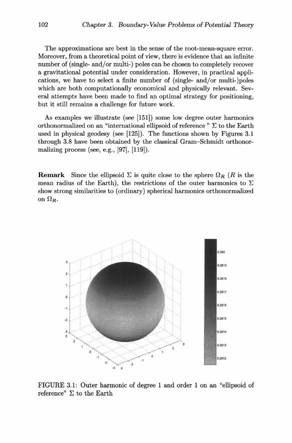
As examples we illustrate (see [151]) some low degree outer harmonics orthonormalized on an "international ellipsoid of reference " ~ to the Earth used in physical geodesy (see [125]). The functions shown by Figures 3.1 through 3.8 have been obtained by the classical Gram-Schmidt orthonormalizing process (see, e.g., [97], [119]).
Remark Since the ellipsoid ~ is quite close to the sphere DR (R is the mean radius of the Earth), the restrictions of the outer harmonics to ~ show strong similarities to (ordinary) spherical harmonics orthonormalized on DR .
. , ·l
FIGURE 3.1: Outer harmonic of degree 1 and order 1 on an "ellipsoid of reference" ~ to the Earth
3.2. Exterior Dirichlet and Neumann Problem 103
0.1
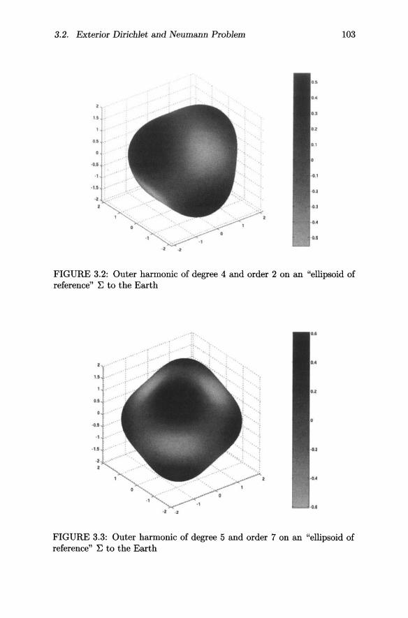
FIGURE 3.2: Outer harmonic of degree 4 and order 2 on an "ellipsoid of reference" E to the Earth
u
D.S
·1
.1.1
·2
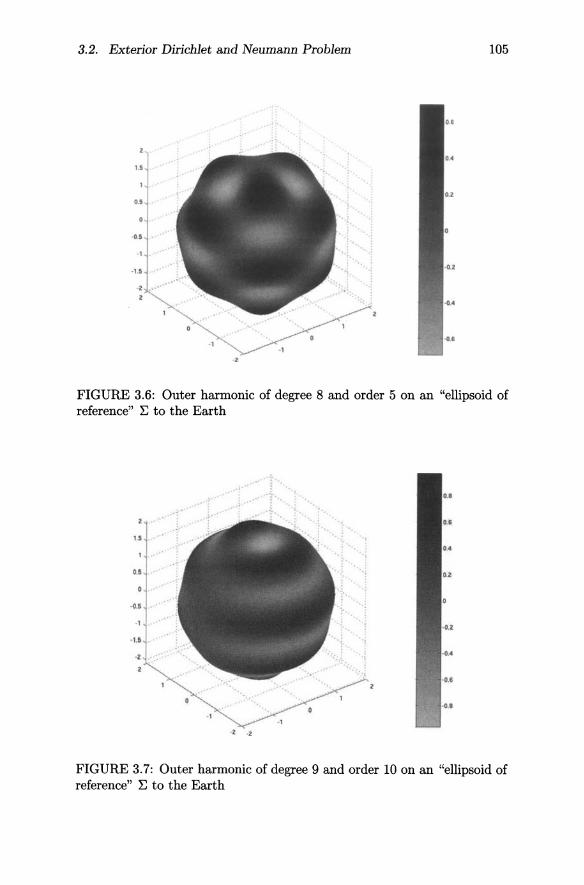
FIGURE 3.3: Outer harmonic of degree 5 and order 7 on an "ellipsoid of reference" E to the Earth

104 Chapter 3. Boundary-Value Problems of Potential Theory
05
....
. ,. ·z
·1lI
·z -l
FIGURE 3.4: Outer harmonic of degree 6 and order 4 on an "ellipsoid of reference" ~ to the Earth
-2 .2
FIGURE 3.5: Outer harmonic of degree 6 and order 10 on an "ellipsoid of reference" ~ to the Earth
3.2. Exterior Dirichlet and Neumann Problem 105
· l
·z
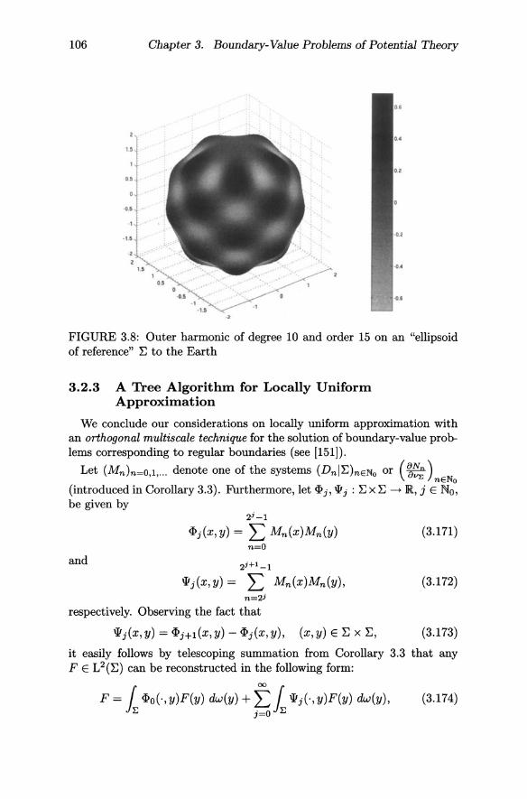
FIGURE 3.6: Outer harmonic of degree 8 and order 5 on an "ellipsoid of reference" E to the Earth
-u .,
. 1.&
·z
·l -l
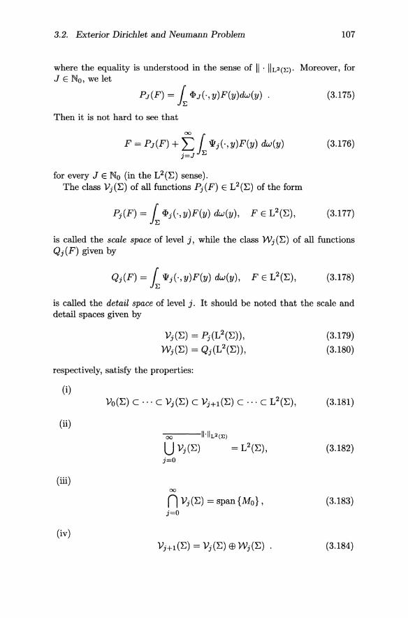
FIGURE 3.7: Outer harmonic of degree 9 and order 10 on an "ellipsoid of reference" E to the Earth
106 Chapter 3. Boundary-Value Problems of Potential Theory
FIGURE 3.8: Outer harmonic of degree 10 and order 15 on an "ellipsoid of reference" E to the Earth
3.2.3 A Tree Algorithm for Locally Uniform Approximation
We conclude our considerations on locally uniform approximation with an orthogonal multiscale technique for the solution of boundary-value problems corresponding to regular boundaries (see [151]).
Let (Mn)n=O,l, ... denote one of the systems (DnIE)nENo or (~~;;) nENo
(introduced in Corollary 3.3). Furthermore, let <I> j, \]i j : Ex E -+ JR, j E No, be given by
2i -1
<I>j(X, y) = L Mn(x)Mn(Y) (3.171) n=O
and 2i+l_1
\]ij(X,y) = L Mn(x)Mn(Y), (3.172) n=2i
respectively. Observing the fact that
\]ij(x,y) = <I>j+1(X,y) - <I>j(x,y), (x,y) E E x E, (3.173)
it easily follows by telescoping summation from Corollary 3.3 that any FE L2(E) can be reconstructed in the following form:
F = ~ <I>o(·, y)F(y) d;.,;(y) + t, ~ \]ij(., y)F(y) d;.,;(y), (3.174)
3.2. Exterior Dirichlet and Neumann Problem 107
where the equality is understood in the sense of II . IIL2(E). Moreover, for J E No, we let
Then it is not hard to see that
F = PJ(F) + f ( Wj(-' y)F(y) dw(y) j=JJE
for every J E No (in the L2(E) sense). The class Vj(E) of all functions Pj(F) E L2(E) of the form
(3.175)
(3.176)
(3.177)
is called the scale space of level j, while the class Wj (E) of all functions Qj(F) given by
(3.178)
is called the detail space of level j. It should be noted that the scale and detail spaces given by
Vj(E) = Pj (L2 (E)),
Wj(E) = Qj(L2(E)),
respectively, satisfy the properties:
(i)
(ii) 00 lI'II L 2(E)
U Vj(E) = L2(E), j=O
(iii) 00 n Vj(E) = span {Mo} ,
j=O
(iv)
(3.179)
(3.180)
(3.181)
(3.182)
(3.183)
(3.184)
108 Chapter 3. Boundary-Value Problems of Potential Theory
The orthogonal sum (3.184) may be interpreted in the following way: The set Vj(~) contains all Prfiltered versions of a function belonging to L2(~). The lower the scale j, the stronger the intensity of filtering (smoothing). By adding "details" contained in the detail space Wj(~) the space Vj+1(~) is created, which consists of a filtered ("smoothed") version at resolution j + 1. It turns out that PH1 = P j + Qj. Note that a collection of (nested) subspaces of L2(~) satisfying (3.181) and (3.182) is called a multiresolution analysis of L2(~).
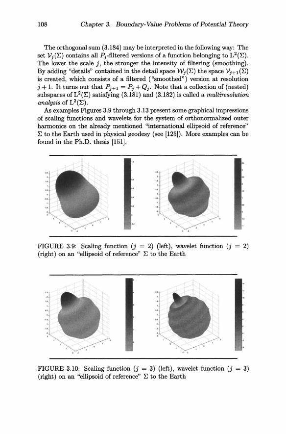
As examples Figures 3.9 through 3.13 present some graphical impressions of scaling functions and wavelets for the system of orthonormalized outer harmonics on the already mentioned "international ellipsoid of reference" ~ to the Earth used in physical geodesy (see [125]). More examples can be found in the Ph.D. thesis [151].
FIGURE 3.9: Scaling function (j = 2) (left), wavelet function (j 2) (right) on an "ellipsoid of reference" ~ to the Earth
.. FIGURE 3.10: Scaling function (j = 3) (left), wavelet function (j = 3) (right) on an "ellipsoid ofreference" ~ to the Earth
3.2. Exterior Dirichlet and Neumann Problem 109
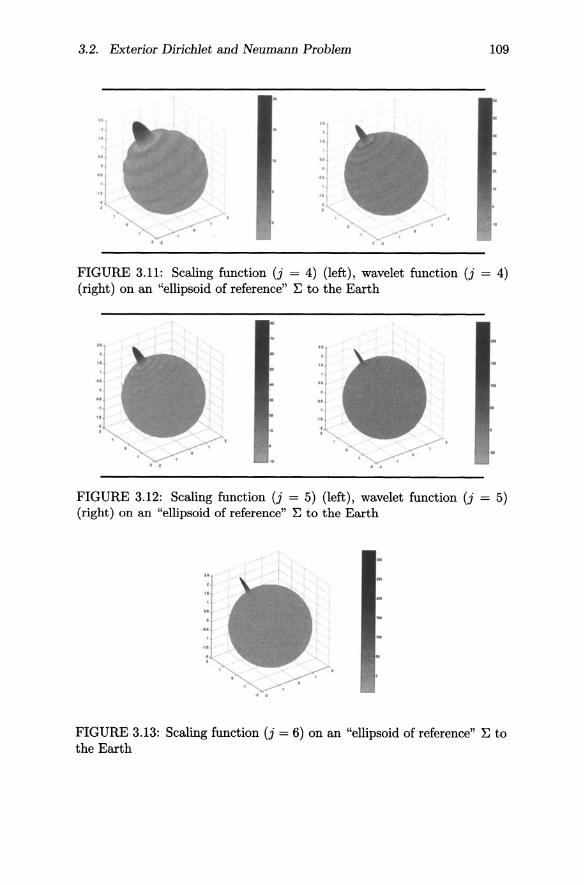
FIGURE 3.11: Scaling function (j = 4) (left), wavelet function (j = 4) (right) on an "ellipsoid of reference" ~ to the Earth
FIGURE 3.12: Scaling function (j = 5) (left), wavelet function (j = 5) (right) on an "ellipsoid of reference" I: to the Earth
FIGURE 3.13: Scaling function (j = 6) on an "ellipsoid of reference" ~ to the Earth

110 Chapter 3. Boundary-Value Problems of Potential Theory
What we are going to realize for a multiresolution analysis as presented above is a tree algorithm (''pyramid scheme") with the following ingredients: Starting from a sufficiently large J such that the difference of F(y) and PJ(F)(y) is negligible for all y E I: (Le., F ~ PJ(F) on I:) and
PJ(F)(x) = l iPJ(x,y)F(y) dw(y) (3.185)
we want to show that coefficient vectors aNj = (ai'\ ... , a~j)T E JRNj , J
j = 0, ... , J - 1 (being, of course, dependent on the function F under consideration) can be calculated such that the following statements hold true:
• For j = 0, ... , J
N· 1 iPj(x,y)F(y) dw(y) ~ tiPj (x,y{"j) a{"j E ~l
• For j = 0, ... , J - 1
• The vectors aNj , j = 0, ... , J - 1, are obtainable by recursion from the vector aNJ .
The essential tools are approximate integration formulae with respect to the system (Mn)n=O,l, ... , Le., we assume that, for j = 0, ... , J, the generating coefficients bfj E JR and the nodal points yfj E I: of the integration formulae are determined such that
N l P(y)Q(y) dw{y) ~ tbfj P (yfj) Q (yfj) (3.186)
holds, e.g., for all P, Q E span (Mo, ... , M21+1-1). Note that the approximate integration formulae of type (3.186) certainly are the most critical point in our construction.
Our considerations are divided into the following two parts, viz., the initial step concerning the scale level J and the pyramid step establishing the recursion relation.
The Initial Step. For an appropriately large integer J, the J-level approximation PJ{F), given by (3.175), is sufficiently close to F E L2(I:). Formally stated,
F ~ PJ{F) = l iPJ(.,y)F(y) dw(y) (3.187)

3.2. Exterior Dirichlet and Neumann Problem 111
implies NJ
F ~ L bf'J q> J (., y{"J) F (y{"J) , (3.188) 1=1
hence, NJ
F ~ L a{"J q> J C, y{"J) (3.189) 1=1
According to (3.186) the coefficients aNJ = (aj""J, ... , a~~)T E ~NJ are given by
a["J=b["JF(y["J), i=1, ... ,NJ . (3.190)
In other words, the coefficients a["J are simply determined by a "read-in"procedure from the functional values of F.
The Pyramid Step. The essential observations for the development of a pyramid scheme are the formulae
(3.191)
and
(3.192)
for j = 0, ... , J. Observing our approximate integration formula (3.186) we, therefore, obtain in connection with the identity (3.191)
where
~ q>j(-' z)F(z) dw(z)
= ~ ~ q>j(-' y)q>j(Y, z) dw(y)F(z) dw(z)
= ~ ~ q>j(y, z)F(z) dw(z)q>j(·, y) dw(y)
N j
~ Larjq>j C,y~j), 1=1
N N· r (N.) ai J = bi J IE q>j Yi J, Z F(z) dw(z),
i = 1, ... , N j , j = 0, ... , J - l.
(3.193)
(3.194)
Next it follows by use of our approximate integration formula (3.186) and the identity (3.192) that
N N r (N.) ai J = bi J Jr:. q>j Yi J, Z F(z) dw(z) (3.195)
112 Chapter 3. Boundary-Value Problems of Potential Theory
= bfi ~~ <I>j (yfi,W) <I>j+l(W,Z) dw(w)F(z) dw(z)
= bfi ~ ~ <I>j+l(W, z)F(z) dw(z)<I>j (yfi, w) dw(w)
NHl bNi '" bNi+l ('" (Ni+l) F( ) dw( )'" (Ni NHl) ~i ~I JE'J!'j+lYI ,z Z z'J!'jYi'YI
N i +l
= bfi L a~Hl <I> j (yfi, y~Hl) . 1=1
Consequently, the coefficients afJ-l can be calculated recursively starting from the data afJ for the initial level J, afJ-2 can be deduced recursively
from afJ - l , etc. This leads us to the formulae
N·
Pj(F) = ( <I>j(., y)F(y) dw(y) ~ t <I>j (-, y~i) a~i, JE 1=1
(3.196)
j = 0, ... , J, with afi, j = 0, ... , J - 1, recursively determined by afJ. It should be noted that the identites (3.196) are equivalent to
(3.197)
for n = 0,1, ... , 2j - 1, hence, it also follows that
(3.198)
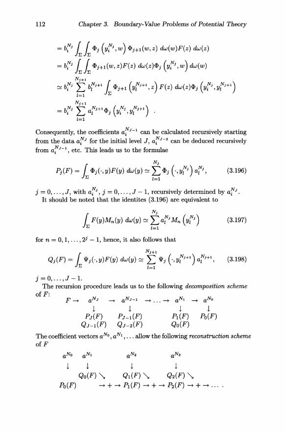
j = 0, ... , J-l. The recursion procedure leads us to the following decomposition scheme
of F:
! PI (F) Qo(F)
! Po(F)
The coefficient vectors aNo , aNl , . .. allow the following reconstruction scheme of F
!! ! ! Qo(F) \. Ql(F) \. Q2(F) \.
Po(F) --t + --t PI (F) --t + --t P2(F) --t + --t ...
3.2. Exterior Dirichlet and Neumann Problem 113
For the pyramid scheme we have to be aware that two sources of errors come into play. First, the input data are already understood to be a filtered version of the input function. Second, an approximate formula is used to establish integration. For a spherical surface E error control (see [21], [64]) shows that both sources, indeed, can be quantified explicitly. Moreover, one can think of several strategies to optimize the reconstruction process. Finally, data compression seems to be performable as long as the coefficients are within a prescribed error threshold.
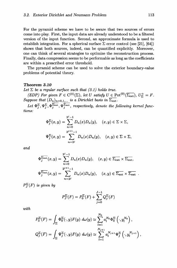
The pyramid scheme can be used to solve the exterior boundary-value problems of potential theory.
Theorem 3.10 Let E be a regular surface such that (3.1) holds true.
(EDP) For given F E C(O)(E), let U satisfy U E Pot(O)(Eext ), ut = F. Suppose that (Dn )n=O,1, ... is a Dirichlet basis in Eext .
Let <pr, wr, <p;ext , w;ext, respectively, denote the following kernel functions:
2j -1
<pr(x,y) = L Dn(x)Dn(Y), (x,y) E E x E, n=O 2j +1 _1
w7(x,y) = L Dn(x)Dn(Y), (x,y) E E x E, n=2j
and
2j-l
<p;ext(x,y) = L Dn(x)Dn(Y), (x,y) E Eext x Eext' n=O 2j +1 _1
w;ext(x,y) = L Dn(x)Dn(Y), (x,y) E Eext x Eext n=2j
PJ (F) is given by
J-1
PJ(F) = P~(F) + L Q7(F) j=O
with
r No
P~(F) = JE <p~(., y)F(y) dw(y) ~ t; a{"o<p~ C, y{"o) ,
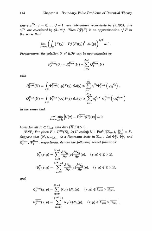
114 Chapter 3. Boundary-Value Problems of Potential Theory
where a~i, j = 0, ... , J - 1, are determined recursively by (3.195), and afJ are calculated by (3.190). Then Py(F) is an approximation of F in the sense that
lim r (F(y) - pY(F)(y))2 dw(y) = 0 ( )1/2
J-+oo 1'2:.
Furthermore, the solution U of EDP can be approximated by
J-1
p;ext (U) = p;ext (U) + L Qyext (U) j=O
with
p;ext(U) = r <fl~ext(.,y)F(y) dw(y) ~ I:,af°<fl~ext (,Yfo), 1'2:. 1=1
Ni+l Qyext(U) = r w;ext(., y)F(y) dw(y) ~ L a~i+lwyext (, yri+ 1 )
1'2:. 1=1
in the sense that
lim sup IU(x) - p;ext(U)(x)1 = 0 J-+OOxEK
holds for all K c Eext with dist (K, E) > O. (ENP) For given FE C(O)(E), let U satisfy U E Pot(1)(Eext ), ~~; = F.
Suppose that (Nn )n=O,1, ... is a Neumann basis in Eext . Let <fly, wy, and
<fl;ext, w;ext, respectively, denote the following kernel functions:
(x,y) E E x E,
(x,y) E E x E,
and
2i_1
<fly ext (x, y) = L Nn(x)Nn(y), (x, y) E Eext x Eext' n=O 2i+l_1
wyext(x,y) = L Nn(x)Nn(y), (x,y) E Eext x Eext . n=2i
3.2. Exterior Dirichlet and Neumann Problem 115
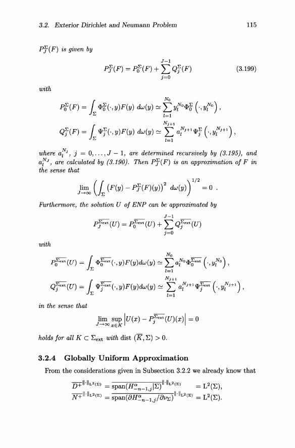
PJ(F) is given by
J-1
PJ(F) = P<f(F) + L Qy(F) (3.199) j=O
with
No
P<f(F) = h CP"f?(., y)F(y) dw(y) ~ ~ yf"OCP"f? (, yf"O) ,
Ni+l
Qy(F) = r 'I!y(., y)F(y) dw(y) ~ L a{"i+1'I!y (, y{"i+l) , JE 1=1
where a{"i, j = 0, ... , J - 1, are determined recursively by (3.195), and af"J, are calculated by (3.190). Then PJ(F) is an approximation of F in the sense that
lim r (F(y) - PJ(F)(y»)2 dw(y) = 0 . ( )1/2
J~oo JE
Furthermore, the solution U of ENP can be approximated by
J-1
pJext (U) = p;ext (U) + L Qyext (U) j=O
with
No
PoEext(U) = r iP"f?ext(·,Y)F(y)dw(y) ~ LafOCP"f?ext (-,yfO), JE 1=1
N i +1
Qyext(U) = r 'I!yext(.,Y)F(Y)dw(Y) ~ L a{"i+1 'I!yext (,y{"i+ 1 ),
JE 1=1
in the sense that
lim sup IU(X) - PjEext(U)(X)1 = 0 J~ooxEK
holds for all K c Eext with dist (K, E) > o.
3.2.4 Globally Uniform Approximation
From the considerations given in Subsection 3.2.2 we already know that
D+II·IIL2(E) = span(H~n_1,jIE)II·IIL2(E) = L2(E),
N + II ·IIL2 (E) _ (;:)Ho j;:) )1I·IIL2(E) _ L2("') - span u -n-1,j UllE - L.. •

116 Chapter 3. Boundary-Value Problems of Potential Theory
Of course, the same results remain valid when the regular surface ~ is replaced by any parallel surface ~(T) of distance ITI to ~ (where ITI is chosen sufficiently small).
This fact will be exploited now to verify the following closure properties (see [50]).
Theorem 3.11 Let ~ be a regular surface satisfying {3.1}. Then the following statements are true:
{i} (H~n-1,jl~) is closed in D+ = c(O)(~):
D+ = span(H~n_1,jl~)II'lIc(o)(}::) = C(O)(~),
{ii} (8H~;;1,j) is closed in N+ = C(O) (~):
N+ = span(8H~n_1,j/8v~)II'lIc(o)(E) = C(O)(~)
PROOF We restrict ourselves to statement (i). Let F be an element of D+. Then the operator equation between F and the function Q of a layer potential of type (3.108) is given by
F = (27rl + P + Fh(O, O))Q . (3.200)
Since we know that P I2 (0, 0) = 111 (0,0)* this equation is equivalent to
-F=(-27ri-P-111(0,0)*)Q. (3.201)
According to the limit formulae of the adjoint operators it follows that
IIL2(T)*Qllc(o)(~) (3.202)
= 11P11(-T,0)*Q -111(0,0)*Q - 27rQllc(o)(~) ~ 0, T ~ 0, T > ° . In connection with our operator equation this means that
11111( -T, O)*Q - F + PQllc(o)(~) -+ 0, T -+ 0, T > ° We now show that the integral extended over the surface ~
R 1(-T,0)*Q(X)=- (Q(y)v(Y)'(Y-TV(Y)-X) dJ..J(y) I J~ IY - TV(Y) - xI 3
(3.203)
(3.204)
can be expressed as an integral over the parallel surface ~(-T). To this end we observe that, for sufficiently small T, the surface element dJ..J_ r of ~(T) may be written in the form
(3.205)

3.2. Exterior Dirichlet and Neumann Problem 117
where H is the mean curvature and L is the Gaussian curvature (see [178]). Since the normals of the parallel surfaces E( -T) coincide with the normals on E, a simple transformation gives
PI1(-T,0)*Q(x) = - r QT(Y)V(~)' (Ypx) dw_T(y) JE(-T) Y - x
1 {) 1 = QT(Y)~( ) -I -I dw_T(y),
E(-T) uvy X-Y (3.206)
where we have introduced as an abbreviation
Q Q(x + TV(X)) T(X) = 1 + 2H(x + TV(X))T + L(x + TV(X))T2
(3.207)
Pjl (-T, 0)* thus can be regarded as the double-layer potential operator with "density" QT on the (inner) parallel surface E( -T).
Furthermore, according to (3.203), (PI1(-T, 0)* +P)Q ~ F in the norm 11'llc(o)(E) as E( -T) ~ E. Therefore, for given c > 0, we can find a surface E( -To:) such that
c IIPjl(-To:,O)+PQ-FIIc<O)(E) ~"2 . (3.208)
Denote by F -To the restriction of the potential
U_ Te (x) = ~(-TO) QT. (y) ({)v~y) Ix ~ YI + I!I) dwTe (y) (3.209)
on the surface E(-T,,), i.e., F_To = U-ToIE(-T,,). The function F_To is continuous on E( -T,,) (see, for example, [170]) and the potential U_ To represents the solution of Dirichlet's exterior problem corresponding to the boundary ~ ( -T,,) and the "boundary function" F -Te . According to our assumption (H~n_l,jIE( -To:»n=O,1, ... ,j=1, ... ,2n+l is closed in L2(E( -T,o). Consequently, the same arguments as used in Subsection 3.2.2 show that there exist an integer m( = m( c» and real numbers an,j such that the inequalities
and
m 2n+l sup U_To(x) - L L an,j H~n_l,j(X) xEr n=O j=l
(3.210)
m 2n+l F_T.{y) - L L an,jH~n_l,j(Y)
n=O j=l

118 Chapter 3. Boundary-Value Problems of Potential Theory
hold for each (compact) subset r of the outer space of the parallel surface ~(-r",) with dist(r, ~( -r",)) > O. In particular, for a set r with dist(r, ~(-r",)) > 0 and ~ c r we get
m 2n+l
sup U_rJx) - L L an,jH~n_l,j(X) ::;~. xEr n=O j=l
(3.211)
Observing the relations (3.208) and (3.211) we thus have
m 2n+l
sup F(x) - L L an,jH~n_l,j(X) xEE n=O j=l
(3.212)
::; sup IF(x) - U-r.(x)1 xEE
m 2n+l
+ sup U_rJx) - L L an,jH~n_l,j(X) ::; c. xEE n=O j=l
This proves Theorem 3.11 (i). I
Remark The same arguments leading to the C-closure of harmonics on ~ apply to all other systems for which L2-closure (on parallel surfaces) is known.
Combining the norm estimates (3.121), (3.122), and the results of Subsection 3.2.2 we easily arrive at the following theorem.
Theorem 3.12 Let ~ be a regular surface satisfying {3.1}. Then the following statements are valid: {EDP} For given F E D+ = C(O)(~), let U satisfy U E Pot(O)(~ext)' ut = F. Then, to every c > 0, there exist an integer m = m(c) and a finite set of a real numbers an,j such that
m 2n+l
sup U(x) - L L an,jH~n_l,j(X) xEEext n=O j=l
m 2n+l
::; sup F(x) - L L an,jH~n_l,j(X) xEE n=O j=l
3.3. Exterior Oblique Derivative Problem 119
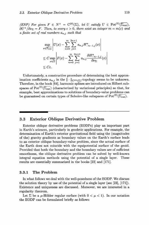
(ENP) For given F E N+ = c(O) (1::), let U satisfy U E Pot (1) (1::ext)' 8U+ 18v};. = F. Then, to every e > 0, there exist an integer m = m(e) and a finite set of real numbers an,j such that
m 2n+1 sup U(x) - L L an,jH~n_1,j(X)
xEEext n=O j=l
m 2n+1 8HQ .
::; C sup F(x) - L L an,j ;;;-1,) (x) xE};. n=O j=l };.
::; Ce.
Unfortunately, a constructive procedure of determining the best approximation coefficients an,j in the II· Ilc(o)(};.)-topology seems to be unknown. Therefore, in the book [64], harmonic splines are introduced on Hilbert subspaces of Pot(O) (1::ext ) (characterized by variational principles) so that, for example, best approximations to solutions of boundary-value problems can be guaranteed on certain types of Sobolev-like subspaces of Pot(O) (1::exd.
3.3 Exterior Oblique Derivative Problem
Exterior oblique derivative problems (EODPs) play an important part in Earth's sciences, particularly in geodetic applications. For example, the determination of Earth's exterior gravitational field using the (magnitudes of the) gravity gradients as boundary values on the Earth's surface leads to an exterior oblique boundary-value problem, since the actual surface of the Earth does not coincide with the equipotential surface of the geoid. Provided that both the boundary and the boundary values are of sufficient smoothness, the oblique derivative problem can be solved by well-known integral equation methods using the potential of a single layer. These results are essentially summarized in the books [23] and [171].
3.3.1 The Problem
In what follows we deal with the well-posedness of the EODP. We discuss the solution theory by use of the potential of a single layer (see [23], [171]). Existence and uniqueness are discussed. Moreover, we are interested in a regularity theorem.
Let 1:: be a f.£-H6Ider regular surface (with 0 < f.£ < 1). In our notation the EODP can be formulated briefly as follows:
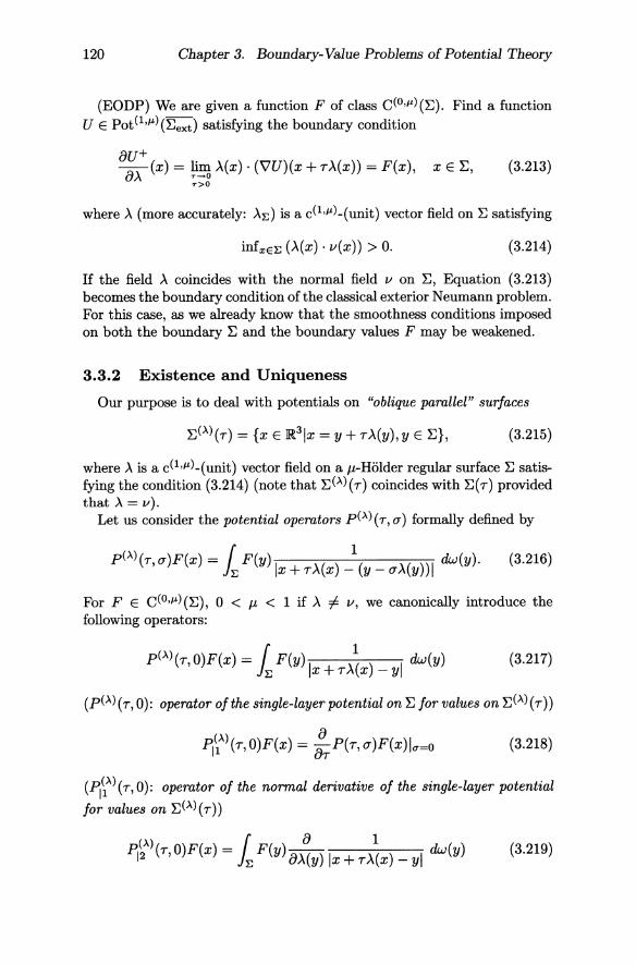
120 Chapter 3. Boundary-Value Problems of Potential Theory
(EODP) We are given a function F of class C(O,J.L)(~). Find a function U E Pot(l,J.L) (~ext) satisfying the boundary condition
au+ aA (x) = ~~ A(X) . (V'U)(x + rA(x)) = F(x), x E ~,
T>O
(3.213)
where A (more accurately: AE) is a c(1,J.LL(unit) vector field on ~ satisfying
infxEE (A(X) . v(x)) > O. (3.214)
If the field A coincides with the normal field v on ~, Equation (3.213) becomes the boundary condition of the classical exterior Neumann problem. For this case, as we already know that the smoothness conditions imposed on both the boundary ~ and the boundary values F may be weakened.
3.3.2 Existence and Uniqueness
Our purpose is to deal with potentials on "oblique parallel" surfaces
~(A)(r) = {x E ~31x = Y + rA(Y), Y E ~}, (3.215)
where A is a c(1,J.LL(unit) vector field on a It-Holder regular surface ~ satisfying the condition (3.214) (note that ~(A)(r) coincides with ~(r) provided that A = v).
Let us consider the potential operators p( A) ( r, a) formally defined by
(A) _ ( 1 P (r,a)F(x)- JEF(Y)lx+rA(x)-(y-aA(Y))1 dw(y). (3.216)
For F E C(O,J.L)(~), 0 < It < 1 if A =f. v, we canonically introduce the following operators:
(A) -1 1 P (r,O)F(x) - F(y) I A() I dw(y) E x+r x -y
(3.217)
(p(A)( r, 0): operator of the single-layer potential on ~ for values on ~(A) (r))
(A) a Fjl (r,O)F(x) = ar P(r, a)F(x)lo-=o (3.218)
(FjiA)(r,O): operator of the normal derivative of the single-layer potential
for values on ~(A)(r))
(A) (a 1 P I2 (r,O)F(x) = JEF(y)aA(y)lx+rA(x)-yl dw(y) (3.219)
3.3. Exterior Oblique Derivative Problem 121
(Fj~A) (7,0): operator of the double-layer potential on ~ for values on the surface ~(A)(7)).
Analogously, FjiA) (0, 0) and Fj~A) (0,0) are introduced formally as (strong-
ly) singular integrals, where FjiA) (0,0) is understood, as usual, in the sense of Cauchy's principal value (see, for example, [171]).
Suppose now that, for sufficiently small values 7 > 0, F E C(O,Jl) (~), ° < J.l < 1 if A =I- v, and x E ~, the operators (L;)(A)(7), (Ji )(A)(7), i = 1,2,3, are defined as follows:
((Lt)(A)(7)) F(x) = (p(A) (±7,0) - P(O, 0)) F(x), (3.220)
((L~)(A)(7)) F(x) = (FjiA) (±7, 0) - FjiA) (0, 0) ± 27r(A(X) . v(x))) F(x),
(3.221)
((Lf)<A) ( 7)) F(x) = (Fj~A) (±7, 0) - p[~A\O, 0) =F 27r(A(X) . v(x))) F(x),
(3.222)
((Jl)(A) (7)) F(x) = (p(A)(7,0) - p(A)(-7,0)) F(x), (3.223)
((h)(A) (7)) F(x) = (FjiA) (7,0) - p[iA) (-7,0) + 47r(A(X) . v(x))) F(x),
(3.224)
((JdA) (7)) F(x) = (Fj~A) (7,0) - Fj~A\ -7,0) - 47r(A(X) . v(x))) F(x).
(3.225)
Observe that (L;)(v)(7) = L;(7), (Ji )(v)(7) = Ji (7),i = 1,2,3. In [77], [79], and [80) it has been verified that the relations
(3.226)
(3.227)
hold for all F E C(O'Jl)(~) and all values J.l' with J.l' < J.l < 1, whereas the relations (with A = v)
(3.228)
(3.229)
are valid for all F E C(O,Jl) (~) and all values J.l' with J.l' :::; J.l < 1.
122 Chapter 3. Boundary-Value Problems of Potential Theory
Observing the norm estimate (3.33) this immediately implies
(3.230)
(3.231)
Furthermore, we have
(3.232)
(3.233)
for all F E C(O,{t)(~).
Let ~ be a J.l-Holder regular surface (0 < J.l < 1). The uniqueness of the EODP can be based on the extremum principle of Zaremba and Giraud (see [23], [137]) in connection with the regularity condition imposed on U at infinity.
In order to prove the existence of the solution we use a single-layer potential
P(O,O)Q(x) = U1(x) = ( Q(Y)-I _1_1 d;.;.;(y) , JE x - y ,
Observing the discontinuity of the directional derivative of the single-layer potential (see (3.221) and (3.226)) we obtain for each Q E C(O,{t) (~) and all points x E ~
(* 8 1 27fQ(x)(>.(x) . lI(x)) + JE Q(y) 8>.(x) Ix _ yl d;.;.;(x) (3.235)
= BUt( ) 8>. x
= F(x)
The resulting integral equation
T(Q) = F, Q E C(O,{t)(~), (3.236)
with
(* 8 1 (TQ)(x) = 27f(>'(x)· lI(x))Q(x) + JE Q(y) 8>.(x) Ix _ yl d;.;.;(y) (3.237)
is of singular type, since the integrals with the asterisk exist only in the sense of Cauchy's principal value. However, Miranda [171] showed, with >.
3.3. Exterior Oblique Derivative Problem 123
of class c(1,I") satisfying (3.214), that all standard Fredholm theorems are still valid (see, e.g., [23], [171]).
As is well known (see, e.g., [23]), the homogeneous integral equation corresponding to (3.236) has no solution other than Q = O. Thus, the solution of the scalar EODP exists and can be represented by a single-layer potential ofthe form (3.234). For more details the reader is referred to, e.g., [23] and [171]. The operator T and its adjoint operator T* (with respect to the L2(~)-scalar product in C(O'I")(~)) form mappings from C(O'I")(~) into C(O,I") (~), which are linear and bounded with respect to the norm 1I·llc(o,I')(E) (see, e.g., [198)). The operators T, T* in C(O'I")(~) are injective and, by Fredholm's alternative, bijective in the Banach space C(O'I")(~) (see [23], [171]). Consequently, by virtue of the open mapping theorem, the operators T-l, (T*)-l are linear and bounded with respect to 11·llc(o,I')(E). Furthermore, (T*)-l = (T- 1)*. Then, in accordance with a technique due to [144] (see also the approach developed in [178]), both T- 1 and (T*)-l are bounded with respect to the norm II ·IIL2(E) in C(O'I")(~).
3.3.3 L2-Closure
Next we consider the pre-Hilbert space (C(O'I")(~), 11·llv(E»). Our aim is to prove a closure theorem by use of a Hahn-Banach argument (see, e.g., [132]).
Theorem 3.13 Let ~ be a regular surface such that (3.1) is true. Then the linear space
apot(O)(~) = {au+ I u P (O)(-A )} a>'E a>'E E ot ext
(3.238)
is a dense subspace of the pre-Hilbert space (C(O'I")(~), II ·11L2(E»).
PROOF Since U E Pot(Aext) has derivatives of arbitrary order in a neighborhood of~, both 'VU and U are p,-Holder continuous on~. The p,-Holder continuity of the vector field>. then shows us that our linear space 8Pot(O) (~) (0 ) ( )
8 A'E ext is a subspace of C ,I" ~.
Let now F be a continuous linear functional on (C(O'I")(~), II·IIV(E») with
(0) -FI aPota>.~Aext) = 0 . (3.239)
We have to prove that F is the zero functional. For each x E Aint the function
(3.240)
124 Chapter 3. Boundary-Value Problems of Potential Theory
apot(O) (if-) belongs to aAE ext • In other words,
(3.241)
Now it is easily seen that the function
x E ~int' (3.242)
is a solution of the Laplace equation in ~int. Note that any differential operator related to x can be interchanged with F, for instance, with fixed x E A int , the function ~(Qx+n;i - Qx) converges to a~i Qx with respect to 1I'llv(E) for r ---- O. Consequently, x f--+ F(Qx), x E A int , is analytic in ~int. Observing ~ext C Aext we obtain Aint C ~int' and by analytic continuation
(3.243)
We specialize the last relation to inner "oblique parallel" surfaces, i.e., to the points x = y - r).,(y), y E ~, r > O. Then we multiply by an arbitrary function G E C(O,JL)(~) and integrate over the regular surface~. As a result we obtain
[ G(y)F (Qy-rA(Y)) m.v(y) = 0, r > 0 . (3.244)
The mapping Ar : ~ ---- C(O,JL)(~) defined by
Y f--+ Ar(Y) = Qy-rA(Y)' y E E, (3.245)
is continuous (note that IIQy-rA(y) - QYO-rA(Yo) IIL2(E) ---- 0 for y ---- Yo on ~ with r > 0 fixed). Consequently, Ar(Y) is integrable. Thus we obtain
F ([ G(y)Qy-rA(y) m.v(y)) (3.246)
= [ G(y)F (Qy-rA(y)) m.v(y)
=0
For G E C(O,JL) (~), we let
U(x) = P(O,O)G(x) = r G(Y)-I _1_1 dw(y), JE x-y
(3.247)
x E ~ext'
_ (A) _ r 1 Ur(x)-P (O,r)G(x)- JEG(y)lx-(y-r).,(y))1 m.v(y), (3.248)
x E ~ext.
3.3. Exterior Oblique Derivative Problem 125
From [79] we know that the limit relation
aUT au+ -- -+ -- T -+ 0, a)..~ a)..~'
(3.249)
holds in the sense of II . IIL2(~). By virtue of (3.249) and (3.246) it now follows that
F (au+) = lim F (aUT) a)..~ T~O a)..~
T>O
(3.250)
= lim F ( r G(y)QY-TA(Y) dw(Y)) :;:g JE =0
for every potential U with a single-layer G E c(O,/L) (:E). Since the space of boundary values ~~; of such potentials is exactly equal to c(O,/L) (:E) (note
that the operator T is bijective), we have the required result F = o. I
3.3.4 A Regularity Theorem
Next we prove a regularity theorem which establishes the well-posedness of the oblique derivative problem.
Theorem 3.14 Let U E Pot(l,/L) (:Eexd be the uniquely determined solution of the EODP corresponding to the boundary values (3.213). Then
holds for all K C :Eext with dist(K,:E) > 0 and all kENo.
PROOF According to our approach, U admits a representation as a single-layer potential (3.234). For each subset K C :Eext with positive distance to :E the estimate
:~~ I (V(k)U) (x) I ::; :~~ (~ ( V1k) Ix ~ vi) , dw(y f' IIQIIL'("I
~ C*(k; K,:E) !!T- 1 (~~:) L2(~) (3.251)

126 Chapter 3. Boundary-Value Problems of Potential Theory
holds (with C*(k; K, 'L.) < 00). By virtue of the boundedness of T- 1 it follows that there exists a constant C( = C(k; K, 'L.)) such that
sup I (V'(k)U) (x)1 ~ C II ~~+ II ' xEK U"E L2(E)
as required. I
3.3.5 L2-Approximation
The point of departure for our considerations concerning L2-approximation is the following theorem.
Theorem 3.15 Let (Dn)n=O,1, ... C Pot(O)(Aext ) be a Dirichlet basis in Aext (see Corollary 3.3). Then the linear space
s an __ n ( 8D+) P n=O,1,... 8AE
is dense in the pre-Hilbert space (C(O,I') ('L.), 11·11L2(E»).
PROOF Given c > 0, F E C(O,I')(E), there exists by Theorem 3.13, a U E Pot(O) (Aext) such that
(3.252)
On the other hand, we know from Corollary 3.4 that there exists a function V E spann =O,1, ... (Dn) with
c/2 ~~~ I (V'U) (x) - (V'V) (x)1 ~ 11'L.1I1/2
Consequently, it follows from (3.253) that
( )1/2 8U+ 8V+ 2 r (-(y) - -(y)) dw(y) ~ ~
JE 8AE 8AE 2
(3.253)
(3.254)
Combining our results via the triangle inequality we therefore obtain the estimate
(3.255)
3.4. Runge-Walsh Approximation by Fourier Expansion 127
as required. I
For numerical purposes (see also [55], [77], [86]) we orthonormalize the
system (~~;;) obtaining the following systems: E n=O,l, ...
• a closed and complete orthonormal system {Dn(~; ·)}n=O,l, ... in the pre-Hilbert space (C(O'IL)(~), 11'IIL2(E»),
• corresponding solutions {Dn(~; ·)}n=O,l, ... to the EODPs Dn(~;') E
pot(l'IL)(~ext)'O < f.J, < 1, satisfying
8D;t(~; .) = D (~ .. ) 8)...E n, . (3.256)
For U E pot(l,Jl)(~ext)' F = ~~;, the orthogonal (Fourier) expansion
(3.257)
converges to F (in the sense of II . IIV(E»)' From the regularity theorem (Theorem 3.14) it follows that
00
U(x) = L (F,Dn (~; '))V(E) Dn (~;x), xEK, (3.258) n=O
holds uniformly on each subset K of ~ext with a positive distance of K to the boundary~. Truncations of the series expansion (3.258) serve as approximations of U in K c ~ext. Furthermore, a pyramid scheme as proposed in Subsection 3.2.2 can be formulated for solving the EODP.
Remark It should be mentioned that we have restricted ourselves to the geoscientifically relevant exterior boundary-value problems. Obvious modifications yield approximation theorems for the interior case.
3.4 Runge-Walsh Approximation by Fourier Expansion
As we already saw, a significant role in all applications is played by the system of outer harmonics (as defined by (2.255)). In fact, outer harmonics
128 Chapter 3. Boundary-Value Problems of Potential Theory
(i.e., multipoles) form a basis of the usually used reference space Jio(Aext) which is loosely speaking the space of all harmonic functions in the outer space Aext of the sphere A with square-integrable restrictions to A. More explicitly, all geosciences take considerable advantage of the fact that each potential U E Jio (Aexd can be represented as an (orthogonal) Fourier expansion in terms of outer harmonics in the form
00 2n+l
U = '" '" U/\L2(A) (n J')HC> . L...J L....J '-n-l,J' (3.259) n=O j=l
where the "Fourier coefficients" U/\L2(A) (n, j) are given by
U/\L2(A) (n,j) = 1 U(y)H~n_l,j(Y) dw(y) . (3.260)
The quantity
(3.261)
is sometimes called the "energy of the potential" U E Jio(Aext) , and because of the ideally frequency localizing character of outer harmonics the energy of the potential can be canonically separated into the energy of the Harmn(Aext)-spaces. This is an essential reason why the geoscientists work more with the "amplitude spectrum"
{U/\L2(A) (n,j)} . n=O,l, ... 3=1, ... ,2n+l
(3.262)
than with the original "signal" U E Jio (Aexd. The "inverse Fourier transform" (3.259) allows the geoscientists to think of the potential U as a sum of "wave functions" H~n-l,j of different "frequencies."
3.4.1 Motivation
In this chapter our purpose is to explain the role of outer harmonics in the Runge-Walsh approximation concept. Briefly formulated, the Runge-Walsh approximation property means that a given potential V E Pot(O) (~ext) can be approximated in locally uniform topology by another potential U E Pot(O) (Aext), where ~,A are regular surfaces such that ~ext C Aext with dist(~, A) > O. In other words, for the potential V there exists a potential U possessing a larger harmonicity domain such that V can be approximated (with any prescribed accuracy) in a uniform sense on compact subsets of ~ext by the restriction UI~ext. In this respect it is
3.4. Runge-Walsh Approximation by Fourier Expansion 129
worth mentioning (for numerical purposes) that the domain of analyticity of U may be chosen particularly to be the outer space of a sphere A satisfying the condition (3.1). More explicitly, for the function V E Pot(O)(~ext) there exists a potential U E 1to(Aext) such that, for arbitrary e > 0, the absolute error between V and UI~ext is in e/2-accuracy on compact subsets of ~ext. Clearly, the potential U is representable as a Fourier series (3.259) in terms of outer harmonics. Therefore, there exists a bandlimited potential UO, ... ,m E 1to(Aexd of the form
m 2n+l
[J, - '"' '"' UA L2(A) (n ')H'" O, ... ,m - ~ ~ ,] -n-l,j (3.263) n=O j=l
such that U and UO, ... ,m are in e/2-distance on subsets of ~ext with positive distance to~. Altogether, for any number e > 0 and V E Pot(O) (~ext) there exists a bandlimited potential UO, ... ,m E 1to(Aexd of the form (3:263) such that the difference between V and UO, ... ,m is in e-accuracy on subsets of ~ext with positive distance to ~. In particular, the Runge-Walsh property justifies the representation of a potential V E Pot(O) (~ext) by a Fourier expansion of a bandlimited potential (3.263) on compact subsets of ~ext.
However, there are two serious difficulties in the Runge-Walsh procedure of finding a truncated Fourier (orthogonal) expansion (3.263) as a locally uniform approximation of V on ~ext. First, the approach is nonconstructive in the sense that the a priori choice of the integer m in (3.263) is unknown. Second, when solving boundary-value problems we have to express the Fourier integrals (3.260) taken over the sphere A by functional values on the regular surface ~ under consideration.
The layout of this section is follows: First we introduce the Sobolev spaces 1to(Aext) in mathematical terms. Then we deal with the role of outer harmonics within the Sobolev space structure 1to(Aexd. More precisely, Subsection 3.4.2 is concerned with the characterization of 1to(Aexd in a general framework of Sobolev-like spaces. Subsection 3.4.3 gives the definition of product kernels in 1to(Aext). Subsection 3.4.4 discusses signal-tonoise thresholding. In Subsection 3.4.5 we discuss Fourier representations of functions on regular surfaces using outer harmonics. Three variants of exact integration formulae by use of outer harmonics are explained in more detail. As mentioned briefly above, the main idea is to express the Fourier coefficients of a bandlimited potential in terms of linear combinations of linear functionals corresponding to points on the regular surface ~ under consideration by solving additional systems of linear equations. Finally, an exact Runge-Walsh orthogonal (Fourier) approximation of bandlimited potentials in boundary-value problems is described in terms of outer harmonics.
130 Chapter 3. Boundary-Value Problems of Potential Theory
3.4.2 Sobolev Spaces
Let (An)nENo be a real sequence. The sequence (An)nENo is called (Bn)summable if An #- 0 for all n and the sum
00 B2 :L)2n+ 1) A; n=O n
(3.264)
is finite. A (1)-summable sequence is simply called summable, i.e., An #- 0 for all nand
00 1 2)2n+ 1) A2 n=O n
(3.265)
is finite (see [69]).
3.4.2.1 Definition
For a given (real) sequence (An)n=O,l, ... such that An #- 0 for all n we consider the linear space [ = [((An); Aext) c Pot(oo) (Aext) of all potentials U of the form
00 2n+l
U = L L (FT)(U)(n,j)H':n_l,j (3.266) n=O j=l
with
(FT)(U)(n,j) = UA L2(A) (n,j) (3.267)
= (U, H':n-l,j)V(A)
= L U(y)H':n_l,j(y)dw(y)
satisfying 00 2n+l
L L A~ (U, H':n-l,j)~2(A) < 00
n=O j=l
From the Cauchy-Schwarz inequality it follows that
00 2n+l
L L A~ (U, H':n-l,j)V(A) (V, H':n-l,j)L2(A) (3.268) n=O j=l

3.4. Runge-Walsh Approximation by Fourier Expansion 131
for all U, V E c. In other words, the left hand side of (3.268) is finite whenever each member of the right hand side is finite. Therefore, we are able to impose on c an inner product (., ')1t«An);Aexd by letting
00 2n+1
(U, V)1t«An);Aext ) = L L A~ (U,H':.n-1,j)V(A) (V,H':.n-l,j)L2(A) n=O j=l
(3.269) The associated norm is given by
(3.270)
Definition Let (An)n=O,l, ... be a real sequence such that An =I 0 for all n. Then the Sobolev space H (more accurately: H((An); Aext») is the completion of c under the norm II . 111t«An);A.;;~):
H((An); Aexd = c((An); Aext)II·II'H«An);Aext).
H equipped with the inner product (', 'hl«An);Aext ) is a Hilbert space. From the Cauchy-Schwarz inequality it follows that (U, V)?-l«l);Aext ) ex
ists if U E H((An); Aext) and V E H((A;;-l), Aext ). Moreover,
(3.271)
Hence, the inner product (', ')1t((1);Aexd defines a duality of H((An); Aext) and H((A;;-l); Aext ).
For brevity, we let
(3.272)
for each real value of s. In particular,
Ho(Aext) = H ((1); Aext) (3.273)
In what follows we often write Hs (instead of Hs(Aext)) when confusion is not likely to arise.
3.4.2.2 Sobolev Lemma
If we associate to U the series (3.266) it is of fundamental importance to know when the series (3.266) converges uniformly on Aext . The answer is provided by the following lemma which may be interpreted to be an analogue of the Sobolev lemma.
132 Chapter 3. Boundary-Value Problems of Potential Theory
LEMMA 3.5 (Sobolev Lemma) Let the sequence (An )n=O,l,... be (Bn)-summable (with Bn i= 0 for all n). Then each U E 'H((B;;l An); Aexd corresponds to a potential of class Pot (0) (Aext ).
PROOF For each N E N, we have
N 2n+l
L L BnA ;;l H~n_l,j(x)AnB;;l (U, H~n-l,j)L2(A) (3.274) n=O j=l
<_ (n~=o (BAnn) 2 2n+l ) L...J t; (H~n_l,j(x))2
(
CXl 2n+l (A )2 ) ~ t; B: (U, H~n-l,j)~2(A)
< (~2n+ 1 B;) 11U11 -1 _. ~ 41l"a2 A~ 'H((Bn An);Aex.}
This proves Lemma 3.5. I
By similar arguments we obtain the following result (see [100]).
LEMMA 3.6 If U E 'Hs(Aexd , s > k + 1, then U corresponds to a potential of class
(k) --Pot (Aext).
Furthermore, we have (see [100]) the following lemma.
LEMMA 3.7 Suppose that U is of class 'Hs(Aext), s> [l] + 1. Then
N 2n+l sup
XEAext (VlU) (x) - L L (U, H~n-l,j)L2(A) (Vi H~n-l,j) (x)
n=O j=l
holds for all positive integers N (with Vi = 8[1] j(8xd1 (8xd2 (8X3)13, li: non-negative integers, it + h + h = [l]), where C is a positive constant independent of u.
3.4. Runge-Walsh Approximation by Fourier Expansion 133
3.4.2.3 The Sobolev Space 'Ho
As is well known, the outer harmonic Fourier transform FT U t--+
(FT)(U), U E 'Ho, is defined by
(FT)(U)(n,j) = U"L2(A) (n,j) = (U,H~n-1,j)1to' (n,j) EN, (3.275)
with N defined by (2.157). The Fourier transform FT forms a mapping from 'Ho into the space 'Ho(N) of sequences {U"L2(A)(n,j)}(n,j)EN with U"L2(A) (n,j) = (U,H~n-1,j)1to, U E 'Ho, satisfying
00 2n+1 IIUII~o = L IU"L2(A) (n,j)1 2 = L L IU"L2(A)(n,j)1 2 < 00
(n,j)EN n=O j=l (3.276)
Any potential U E 'Ho is characterized by its "amplitude spectrum"
{U"L2(A) (n, j)} (n,j)EN = {(U, H~n-1,j)1tohn,j)EN
More explicitly, for U, V E 'Ho,
N 2n+1 lim U - '" '" (V,H~n-1J·)1toH::'n-1J· N~oo ~~ , ,
=0 (3.277) n=O j=l 1to
we have U = V (in the sense of II . l11to)' In addition, for U E 'Ho,
N 2n+1
J~oo U - L L (U, H::'n- 1,j)1to H::'n- 1,j =0 (3.278) n=O j=1 1to
implies
N 2n+1 J~oo suE. U(x) - L L (U, H::'n- 1,j)1to H::'n_1,j(x) = 0
xEK n=O j=l (3.279)
for all K c Aext with dist(K, A) > O. In particular, we have
N 2n+1
J~oo su~ U(x) - L L (U, H::'n- 1,j)1to H::'n_1,j(x) = 0 xE n=O j=l
(3.280)
for all regular surfaces E satisfying (3.1). Next we consider a potential U E 'Ho of the form (3.266), i.e.,
00 2n+1 U = L L 1 U(y)H::'n_1,j(Y) dw(y)H::'n_1,j .
n=O j=l A
(3.281)
134 Chapter 3. Boundary-Value Problems of Potential Theory
Then the restriction of U to the set ~~~ is given by
-'-f a "inf a n "inf 00 2n+l ( inf)n 1 ul~~~t = L La. U(y)H_n_1,j(Y) dw(y) ( inf) H_n-1,j,
n=O j=l Emf a (3.282)
where we have observed the following identities:
Q () (a) n "inf () H_n-1,j x = a inf H_n-1,j x , E ~inf X Llext' (3.283)
and
1 (ainf)nl' f U(y)H~n_l,j(Y) dw(y) = - . U(y)H':.~_l,j(Y) dw(y) A a Emf
(3.284) for n = 0,1, ... , j = 1, ... , 2n + 1. But this shows us that for all U, V E 'lio
(U, Vhto (3.285) 00 2n+l
= ~ f; i U(y)H~n_l,j(Y) dw(y) i V(y)H~n_l,j(Y) dW(y)
00 2n+l ( inf) 2n1 1 = L L ~ . U(y)H':.:~l,j(Y) dw(y) . V(y)H':.:~l,j(Y) dW(y)
n=O j=1 a Emf Emf
= (U,V)H(((U:fr);E~';!.) .
This yields the remarkable result (see [64]) that
(3.286)
Moreover, it is clear that
(3.287)
for all subsets K c ~~~~.
Theorem 3.16 The space 'liO(Aext)I~~~~ is a Hilbert subspace ofPot(oo)(~~~~). Moreover,
'liO(Aext)I~~';!t has the reproducing kernel function
K ( ) . ~inf X ~inf llJ)
H ( ( ( u:f r) ;E~';,;) ',' . Llext Llext -+ Jl'l,. (3.288)
3.4. Runge-Walsh Approximation by Fourier Expansion 135
given by
00 2n+ 1 a 2n inf inf
KH(((a:fr);E~~~)(x,y) = ~ ~ (ainf ) H':..n-l,j (X)H':..n_l,j (y),
(3.289)
(x, y) E E~'i~ x E~~. The system {H~~~l,j} . n=O,l, ... , , given by {3.283} }=1, ... ,2n+l
represents an 7to(AexdIE~'i~-orthonormal basis. More explicitly, we have the following:
{i} For every fixed y E E~'iL the potential
-- --·-f belongs to 7to (Aext) I E~'it .
{ii} For any U E 7to(AexdIE~'i~ and any point x E E~~ the reproducing property
U(x) = (KH(((ainf)n)'Einf) (.,x),U) . n-a ' ext H ( ( ( a:;'f) ) ;E~~~)
is valid.
Reproducing kernel representations corresponding to certain pointsets may be used to act as a basis system in reproducing Sobolev spaces. To be more specific, we formulate the following theorem.
Theorem 3.17 Assume that X is a countable dense set of points on a regular surface :::: c E~'i~. Then
7to (Aext) IE~~ = 7t (( (~) n) ;~) = spanxEXKH( (( a:fr);E~~~) (., x),
where the completion is understood in the sense of II . IIH(( (a: f r);E~~~)'
PROOF Our purpose is to show that the conditions U E 7to(Aext)IE~'i~ and
o = (K ((( ainf )n) .---y,:;() (., x), U) H <> ,Eext H(((a:fr);E~~~)
(3.290)

136 Chapter 3. Boundary-Value Problems of Potential Theory
for all x E X imply U = O. Clearly, the condition (3.290) is equivalent to U (x) = 0 for all x EX. According to our construction, U is continuous on
3 C ~~'i~. Hence, it follows that if U(x) f= 0 for some x E 3 then U would be different from zero for a neighborhood of x E 3. But this is impossible because of the assumption imposed on X c 3. This proves Theorem 3.17.
I
Obviously, Theorem 3.17 particularly holds for 3 = ~. Moreover, Theorem 3.17 allows an obvious generalization by means of bounded linear
functionals on 1t(Aexdl~~'i~.
Theorem 3.18 Assume that X is a countable set of linear functionals in the dual space
1t ( ( ( l1:f) n) ; ~~';!t) * of 1toCA;'~;) I~. Then
1to (Aext) I~~'i~ = spanCExCK'H((( O":fr);E~~~) (.,.) .
3.4.3 Product Kernels in 1to
Of particular importance for all our further considerations are product kernels of the form
00 2n+l
K(x, y) = L Ii(n) L H':n-l,j (X)H':n_l,j (y), (x, y) E Aext x Aext, n=O j=l
(3.291 ) where Ii(n) are real numbers for n = 0,1, .... Notice that
K(x,y) = K(y,x), (x, y) E Aext x Aext (3.292)
Le., product kernels of the form (3.291) are symmetric. Moreover,
(x, y) f-+ K(x, y), (x, y) E A x A, (3.293)
defines a spherical radial basis function (see Subsection 2.2.3). By virtue of the addition theorem the product kernel K may be rewritten
as follows:
The sequence (KA(n))n=O,l, ... , given by
KA(n) = Ii(n), n = 0,1, ...
is called the symbol of the product kernel K.
(3.294)
(3.295)
3.4. Runge-Walsh Approximation by Fourier Expansion 137
3.4.3.1 1-lo-Kernel Functions and Convolutions
A product kernel K of the form (3.291) is called an 1-lo-kernel (more explicitly, an 1-l~0!'0!) -kernel) if
00 2n+1 L (KA(n))2 L H~n_1,j(x)H~n_1,j(Y) < 00 (3.296) n=O j=1
for all (x, y) E A x A, i.e.,
(3.297)
Let K be an 1-lo-kernel. Suppose that U is of class 1-lo. Then we understand the convolution of K and U to be the function of class 1-lo given by
(K *'Ho U)(x) = (K(x, .), U)'Ho = L K(x, y)U(y) dw(y), (3.298)
x E A ext . Obviously, K *'Ho U is a member of class 1-lo. Furthermore, we have
(FT)(K *'Ho U)(n,j) = (FT)(U)(n,j)KA(n), (n,j) EN .(3.299)
If L is another 1-lo-kernel, then L *'Ho K is defined by
(L *'Ho K)(x, y) = L L(y, z)K(z, x) dw(z), (3.300)
( x, y) E Aext x A ext . It is readily seen that
(3.301)
We usually write K(2) = K *'Ho K to indicate the convolution of a kernel with itself. K(2) is said to be the iterated kernel of K. Obviously, we have
(3.302)
Note that (3.299) and (3.301) justify the name "convolution" for the definitions (3.298) and (3.300), since analogous statements hold in the classical L2(lR.)-case.
3.4.3.2 1-lo-Kernel Representations on Regular Surfaces
Let K be an 1-lo-kernel satisfying KA(n) i=- 0 for all n. Then the following results are known from Subsection 3.2.2:
138 Chapter 3. Boundary-Value Problems of Potential Theory
(EDP) Let {xkh=1,2, ... be a countable dense system of points Xk on a regular surface ~. Then
C("<"') - D+ - (K( )+)II'lIc(o)(E) L..J - ~ - spank=1,2,... ., Xk (3.303)
and
(3.304)
(ENP) Let {xkh=1,2, ... be a countable dense system of points Xk on a regular surface ~. Then
o + (8K(., Xk)+) 11'llc(o)(E) C( ) (~) = N~ = spank=1,2,... 8v~ (3.305)
and
(3.306)
3.4.4 Spectral Signal-to-Noise Thresholding
Thus far only a (deterministic) function model has been discussed. If a comparison of a measured function with the actual function were made, discrepancies would be observed. A mathematical description of these discrepancies has to follow the laws of p~obability theory in a stochastic model.
Usually the observations are not looked upon as a time series, but rather as a function F on the sphere A with radius" a (rv indicator for stochastic). According to this approach we assume (see [73], [81], [94], [194]' [195]) that
(3.307)
where if is the observation noise. Moreover, in our approach, we suppose the covariance to be known
Cov [F(x),F(y)] = E[if(x)J(y)] =K(x,y), (x,y) E Aext x Aext,
(3.308) where K is an ?-lo-product kernel, i.e,
(3.309)
3.4. Runge-Walsh Approximation by Fourier Expansion 139
3.4.4.1 Degree Variances
The signal degree and order variance of P is defined by
Varn,k (p) = (P *Ho H~n-l,kr = (PAL 2(A)(n,k)r (3.310)
= i i p(x)p(y)H~n-l,k(X)H~n_l,k(Y) dw(x) dw(y)
Correspondingly, the signal degree variances of P are given by
2n+l Yarn (p) = L Varn,k (P) (3.311)
k=l 2n+l 2
L (pAL2(A)(n,k)) k=l
2n + 1 r r - - ( x y ) = 47ra2 JA JA F(x)F(y)Pn j;T. TYI dw(x) dw(y),
n = 0,1, .... According to Parseval's identity we obtain for the total variance of P
(3.312)
3.4.4.2 Degree Error Covariances
The error spectral theory is based on the degree and order error covariance
Covn,k(K) = i i K(x, y)H~n-l,k(X)H~n-l,k(Y) dw(x) dw(y), (3.313)
and the spectral degree error covariance
2n+l Covn(K) = L r r K(x, y)H~n-l,k(X)H~n-l,k(Y) dw(x) dw(y)
k=l JA JA
2n+ 1 r r (x y) = 47ra2 JA JA K(x, y)Pn j;T. TYI dw(x) dw(y) . (3.314)
In other words, the spectral degree and order error covariance is simply the orthogonal coefficient of the kernel K.
3.4.4.3 Examples of Spectral Error Covariances
To make the preceding considerations more concrete we would like to discuss two particularly important examples.

140 Chapter 3. Boundary-Value Problems of Potential Theory
(1) Bandlimited white noise. Suppose that for some nK E No
(3.315)
where g is assumed to be N(O, 0-2)-distributed. The kernel reads as follows:
(3.316)
Note that this sum, apart from a multiplicative constant, may be understood as a truncated Dirac a-functional.
(2) Non-bandlimited colored noise. Another geophysically relevant example is the following 1to-kernel:
00 (2 ) n+l 2 + 1 ( ) K(x, y) = ~ KI\(n) I~IYI ~a2 Pn 1:1· I~I ' (3.317)
where KI\(n) 1:- 0 for an infinite number of nand K(x,x) coincides with 0-2 for all x E A, i.e.,
2 = ~ KI\( ) 2n + 1 0- L n 47ra2 •
n=O
(3.318)
From the uncertainty principle (see Subsection 2.2.4) we know that a small "decorrelation length" on A can be assured by assuming
KI\(n) ~ KI\(n + 1) ~ 1 (3.319)
for a large class of (subsequent) integers n.
3.4.4.4 Spectral Estimation
Now we are in position to compare the signal spectrum with that of the noise: The signal and noise spectra "intersect" at the degree and order resolution set N"res with
Nres eN = {(n, k) 1 n = 0,1, ... , k = 1, ... , 2n + I} . (3.320)
We distinguish the following cases:
(i) signal dominates noise
(3.321)
3.4. Runge-Walsh Approximation by Fourier Expansion 141
(ii) noise dominates signal
(3.322)
Filtering is achieved by convolving an 1io-product kernel H with 1io-kernel symbol {HA(n)}n=O,l, ... against F:
P = H *1-lo F = l H(-, y)F(y) dw(y)
(1\ denotes "estimated"). In spectral language this reads
Two important types of filtering should be listed:
(i) Spectral thresholding. We let
00 2n+l
P = L L INres(n, k)HA(n)FAL2cAl (n, k)H'.:n_l,k, n=O k=l
(3.323)
(3.324)
(3.325)
where Ip denotes the indicator function of the set PeN (defined by Ip(n, k) = 1 for (n, k) E P and Ip(n, k) = 0 for (n, k) ¢. P).
This approach represents a "keep-or-kill" filtering (see, e.g., [33]), where the signal dominated coefficients are filtered by an 1io-kernel, and the noise dominated coefficients are set to zero. This thresholding can be thought of as a non-linear operator on the set of coefficients, resulting in a set of estimated coefficients.
As a special filter we mention the ideal low-pass (Shannon) filter H of the form
HA(n, k) = HA(n) = {1 , (n, k) E Nres . 0, (n, k) ¢. Nres
(3.326)
In that case all "frequencies" (n, k) E Nres are allowed to pass unweakened, whereas all other frequencies are completely eliminated.
(ii) Wiener-Kolmogorov filtering. Now we choose (see, e.g., [194])
00 2n+l
P = L L HA(n)FAL2CAl(n,k)H'.:n_l,k (3.327) n=O k=l
with
HA(n) = ~arn(F) Varn(F) + Covn(K)
(3.328)
This filter produces an optimal weighting between signal and noise (provided that complete independence of signal and noise is assumed).
142 Chapter 3. Boundary-Value Problems of Potential Theory
3.4.5 Fourier Representation of Functions on Regular Surfaces
Next we are interested in Fourier representations of functions on regular surfaces. We begin with some preliminary considerations.
Since the set of all finite linear combinations of outer harmonics when restricted to a regular surface ~ (satisfying (3.1)) is uniformly dense in the space C(o)(~), the space 1iol~ is a uniformly dense subset of C(o)(~), too.
Suppose now that there is given a continuous function on a regular surface ~ from which function values are available on a finite set of discrete points of~. Then, an extended version of Helly's theorem (see [222]) shows that, corresponding to this continuous function on ~, there exists a member F of class 1iol~ in an (c/2)-neighborhood that is consistent with the function values of the continuous function on ~ for the known finite set of discrete points. Moreover, this function F of class 1iol~ may be assumed to be in (c/2)-accuracy to a member Fo, ... ,m of class Harmo, ... ,m(~) which can be supposed to be consistent with the known function values as well. In other words, corresponding to any continuous function on a regular surface ~, there exists in c-accuracy a bandlimited function Fo, ... ,m such that this bandlimited function Fo, ... ,m coincides at all given points with the function values of the original continuous function on the regular surface~. This is the reason why we are interested in Fourier approximations of functions Fo, ... ,m of class Harmo, ... ,m(~) from discretely given function values.
To be more concrete, let us assume that there exists an integer m :::: 0 and a potential UO, ... ,m E Harmo, ... ,m(Aext} such that Uo, ... ,ml~ is just equal to the function Fo, ... ,m we are looking for.
We want to present three algorithms showing to obtain Fo, ... ,m from discretely given data on ~ using the Fourier expansion in terms of outer harmonics (see [100]).
3.4.5.1 First Fourier Variant
We need an integration formula for the product of two functions PO, ... ,a E
Harmo, ... ,a(Aext) and QO, ... ,b E HarmO, ... ,b(Aext), i.e., for prescribed nodes Xl, .. " XM E ~, we have to determine the weights al, ... , aM in such a way that
M 1 PO, ... ,a(y)Qo, ... ,b(Y)dw(y) = L arPo, ... ,a(xr)Qo, ... ,b(Xr). A r=l
(3.329)
At first, we investigate the space of all product functions consisting of factors of Harmo, ... ,a(Aext) and HarmO, ... ,b(Aext). Let H~n-l,j' respectively, H~k-l,i denote outer harmonics of degree nand k, respectively. Then it

3.4. Runge-Walsh Approximation by Fourier Expansion 143
is easily seen from [69] that
(3.330)
with coefficients ai,s E JR, l = 0, ... ,n + k, s = 1, ... ,2l + 1, where we have used the abbreviation
It is not difficult to verify that, for each r E N, the members of the system
{P8,1(a; .),PJ,1(a; .), Pi, 1 (a; .), Pl,2(a; .), Pl,3(a; .), PJ,1 (a; .), Pr.1 (a; .)
(3.331) , ... , P;'2r+1 (a; .)}
are linearly independent. Next we consider the space of all product functions with factors of class
Harmo, ... ,a(Aext) and Harmo, ... ,b(Aext), respectively.
LEMMA 3.8 Suppose that PO, ... ,a E Harmo, ... ,a(Aext) and QO, ... ,b E Harmo, ... ,b(Aext). Then the product PO, ... ,aQO, ... ,b is of class
Harmo, ... ,a+b(Aext) = span r=O, ... ,a+b (P{s(a; ,)). l=O, .... r '
(3.332) s=1, ... ,2l+1
The dimension of Harmo, ... ,a+b(Aext) is equal to
PROOF PO, ... ,a E Harmo, ... ,a(Aext) and QO, ... ,b E Harmo, ... ,b(Aext) may be represented in the form
a 2n+1 PO, ... ,a(Y) = L L (PO, ... ,a)/\L2(A) (n,j)H~n_1,j(Y)' Y E Aext'
n=O j=l

144 Chapter 3. Boundary-Value Problems of Potential Theory
and
b 2k+1 QO, ... ,b(Y) = L L (Qo, ... ,b/,'L2(A) (k, i)H~k-1,i(Y)' Y E Aext'
k=O i=l
respectively. Thus, the product PO, ... ,aQO, ... ,b reads as follows:
a+b r 21+1
(PO, ... ,aQO, ... ,b)(Y) = L L L br,sp":s(a; y), Y E ~ext' (3.333) r=O 1=0 s=l
with certain coefficients br s' r = 0, ... ,a + b, 1 = 0, ... ,r, s = 1, ... ,2l + 1.
This proves Lemma 3.8. ' I
Now we are in a position to develop integration rules for members of class Harmo, ... ,a+b(Aext). Basic tools are admissible point systems leading to exact integration formulae.
Definition A setX~ = {xtt", ... ,x~n c~, M = L:~~g(r+1)2, is called a Dirichlet-fundamental system on ~ with respect to Harmo, ... ,a+b(Aext), if the matrix
( P8,1 (a; xtt") P8,l (a; xM) )
· . · . · . a+b . M a+b . M Pa+b,2(a+b)+1 (a, Xl ) ... Pa+b,2(a+b)+1 (a, xM)
is regular.
This definition enables us to derive the following lemma.
LEMMA 3.9 Let PO, ... ,a E Harmo, ... ,a(Aexd and QO, ... ,b E HarmO, ... ,b(Aext). Furthermore, suppose that X~ = {xtt", ... ,xM} c ~, M = L:~~g(r + 1)2, is
a Dirichlet-fundamental system on ~ with respect to Harmo, ... ,a+b(Aexd. Then, the integration formula
M
r PO, ... ,a(y)Qo, ... ,b(Y)dw(y) = L akPo, ... ,a(xr)Qo, ... ,b(Xr) iA k=l
holds for all weights aI, ... , aM satisfying the linear equations
3.4. Runge-Walsh Approximation by Fourier Expansion 145
r = 0, ... ,a + b, l = 0, ... ,r, s = 1, ... ,2l + 1.
Summarizing our results we obtain the following Fourier representation of a function on a regular surface E.
Theorem 3.19 Suppose that the subset X£ = {xr, ... , x~} of E with
2m
M = 2:(r+ 1)2 (3.334) r=O
is a Dirichlet-fundamental system on E with respect to Harmo, ... ,m (Aexd. Furthermore, assume that from a function Fo, ... ,m E Harmo, ... ,m(E) there are known the function values at all points of X£. Then,
m 2n+1 M
Fo, ... ,m(z) = 2: 2: 2: akFo, ... ,m(x~)H':n_1,j(x~)H':n_1,j(z), (3.335) n=O j=1 k=1
Z E E, where the weights a1, ... ,aM have to satisfy the linear equations
(3.336)
r = 0, ... , 2m; l = 0, ... , r; s = 1, ... , 2l + 1.
It should be pointed out that all integration weights can be calculated in an a priori step and stored elsewhere for computations with other selections of input functions. However, much effort is required to solve the large linear system (3.336) (at least for large m).
3.4.5.2 Second Fourier Variant
Next we develop an integration rule of the form
M 1 PO, ... ,a(y)Q(y) dw(y) = 2: ar Po, ... ,a(Xr ),
A r=1 (3.337)
where
{Xl, ... , XM} c E, PO, ... ,a E Harmo, ... ,a(Aext), Q E 1io. (3.338)
Our aim is to reduce the dimension of the linear system determining the integration weights by considering only one factor of the integrand for single point evaluation on the right hand side of (3.337). In doing so we
146 Chapter 3. Boundary-Value Problems of Potential Theory
only have to work with point systems which are admissible for a basis of Harmo, ... ,a(I:exd·
Definition A set X£. = {xr, ... , x~n c I:, M = (a + 1)2, is called a Dirichlet-fundamental system on I: with respect to Harmo, ... ,a(Aext) if the matrix
is regular.
(3.339)
is of maximal rank, hence, the assumption that X£. is a Dirichlet-fundamental system on I: with respect to Harmo, ... ,a(Aext) is equivalent to the regularity of the Gram matrix (3.339).
The preceding definition leads us to the following integration formula.
LEMMA 3.10 Let X£. = {xr, ... ,x~n c I:, M = (a + 1)2, be a Dirichlet-fundamental system on I: with respect to Harmo, ... ,a(I:exd. Furthermore, suppose that PO, ... ,a E Harmo, ... ,a(I:ext) and Q E Ho. Then,
a 2n+l M 1 PO, ... ,a(y)Q(y)dw(y) = L L La~,jQt\L2(A)(n,j)Po, ... ,a(x~) A n=O j=l r=l
holds for all weights a~,j, ... ,ar;j, n = 0, ... ,a, j = 1, ... ,2n + 1 satisfying the linear equations
M
L a~,j H':k_l,i(X~) = 8nk8ji , k = 0, ... ,a, i = 1, ... ,2k + 1. (3.340) r=l
3.4. Runge-Walsh Approximation by Fourier Expansion 147
PROOF By applying the Parseval identity we are able to deduce that
1 PO, ... ,a(y)Q(y) dw(y) (3.341)
a 2k+1
= ~ 8 (PO, ... ,a)"L2(A) (k, i) 1 Q(y)H~k-l,i(Y)dw(y) a 2k+1 a 2n+1
= L L (Po, ... ,a)"L2(A)(k,i) L L Q"L2(A) (n,j)8nk8ji k=O i=l n=O j=l
a 2k+1 a 2n+1 M
= L L (PO, ... ,a)'\L2(A) (k,i) L L La~,jQ"L2(A)(n,j)H~k_l,i(X~) k=O i=l n=O j=l r=l
a 2n+1 M
= L L La~,jQ"L2(A)(n,j)Po, ... ,a(X~). n=O j=l r=l
This verifies Lemma 3.10. I
By inspecting the results of Lemma 3.10 we observe that we have reduced the dimension of the system of linear equations determining the integration weights about one order of magnitude in comparison with Fourier variant 1. The price that must be paid is the solution of (a + 1)2 linear systems to establish exact integration of the product PO, ... ,aQ. A simple idea to reduce the total amount of integration weights is to give up the universal validity of the integration rule.
COROLLARY 3.5 Under the assumptions of Lemma 3.10, the integration formula
M 1 PO, ... ,a(y)Q(y) dw(y) = L arPo, ... ,a(X~) A r=l
holds for all weights al, ... , aM satisfying the linear equations
M
L arH~k_l,i(X~) = Q"L2(A) (k, i), k = 0, ... ,a, i = 1, ... ,2k + 1. r=l
(3.342)
PROOF We let
a 2n+1
ar = L L a~,jQ"L2(A) (n,j), r= 1, ... ,M, (3.343) n=O j=l

148 Chapter 3. Boundary-Value Problems of Potential Theory
and apply Lemma 3.10. I
It should be noted that the number of integration weights is indeed reduced, but that they now depend on Q (see (3.342)).
Summarizing all results of this variant we obtain as a fully discrete Fourier approximation the following theorem.
Theorem 3.20 Let X£ = {xf1", ... , x~n c L:, M = (m + 1)2, be a Dirichlet-fundamental system on L: with respect to Harmo, ... ,m(Aext).
Furthermore, assume that from a function Fo, ... ,m E Harmo, ... ,m(L:) we know the function values at all points of X£. Then
m 2n+i M
Fo, ... ,m(z) = L L L arFo, ... ,m(x~)H~n_i,j(Z), Z E L:, n=O j=i r=i
where the weights ai, ... , aM satisfy the linear equations
M
L arH~k-i,i (x~) = OnkOji' k = 0, ... ,m, i = 1, ... , 2k + 1 r=i
(3.344)
(3.345)
Comparing Fourier variants 1 and 2 we come to the following conclusion: The integration weights of variant 1 depend neither on the analyzed bandlimited function Fo, ... ,m, nor on the outer harmonics under consideration. The disadvantage here (at least for a non-spherical regular surface L:) is the dimension of the product space (note that the dimension of Harmo, ... ,a+b(Aext) generally is of order O((a + b)3)), which might cause huge problems when we attempt to solve the linear systems numerically. In variant 2, the dimension of Harmo, ... ,a(L:ext) is of order O(a2 ), such that higher order systems can be inverted to some extent. On the other hand, one has lost a lot of flexibility in the method.
3.4.5.3 Runge-Walsh Fourier Approximation
We are now interested in a fully discrete Fourier approximation seen from the point of view of potential theory. Since the set of all finite linear combinations of outer harmonics when restricted to L:ext (i.e., the Earth's exterior L:ext including the Earth's surface L:) is uniformly dense in the space Pot (0) (L:ext ), the space 1io \L:ext is a uniformly dense subset of Pot(O) (L:ext ), too. In formulae,
Pot(O)(~)
_ 'LI \"" 11·lIc(o)(Eext) - ,~o Liext
(3.346)
3.4. Runge-Walsh Approximation by Fourier Expansion 149
----------===-I!·IIC(O) (Eext) = span. n=O,l,.. (H~n_l,jl~ext) .
]=1 •... ,2n+l
Suppose now that there is known from a potential V (i.e., the actual Earth's gravitational potential) of class Pot (0) (~ext) a set {VI, ... , V M} of M values Vi, i = 1, ... , M, corresponding to linear (observation) functionals L1, ... ,LM . Then an extended version of Helly's theorem (see [222]) tells us that, corresponding to the potential V E Pot(O) (~ext)' there exists a member U (Le., a Runge-Walsh approximation of the gravitational potential) of class 'lio(Aext) such that UI~ext is in an (c/2)-neigborhood to V (understood in C(~ext)-topology) and LiU = Vi, i = 1, ... , M (note that we may write more accurately Uo, ... ,oo instead of U to indicate that all Harm-spaces generally contribute to the "nature" of U). Moreover, there exists an element UO, ... ,m (i.e., a bandlimited approximation to the RungeWalsh approximation) of class Harmo, ... ,m(~ext) such that Uo, ... ,ml~ext may be considered to be in (c/2)-accuracy to UI~ext uniformly on ~ext and, in addition, LiUO, ... ,m = LiU = Vi, i = 1, ... , M. In other words, corresponding to the potential V E Pot(O) (~ext) there exists in c-accuracy on ~ext a bandlimited potential in 'lio(Aexd, (namely UO, ... ,m E Harmo, ... ,m(Aext» consistent with the original data (Le., Vi = LiU = LiUO, ... ,m, i = 1, ... ,M). This is the reason why we are interested in Fourier approximations of potentials UO, ... ,m of class Harmo, ... ,m(Aext) uniformly on ~ext from a finite set of functional values.
3.4.5.4 Exact (Outer Harmonics) Integration Formulae
As we have said, our purpose is to develop different types of integration formulas. Our starting point is the concept of fundamental systems.
Definition A set {Lj'f, ... , L~}, M = 2:::!(2l+1), of M linearly inde
pendent bounded linear functionals on Harmp, ... ,q(Aext) is called a Harmp, ... ,qfundamental system on ~ext with respect to Harmp, ... ,q(Aext ) if the matrix
(3.347)
is regular.
Obviously,
150 Chapter 3. Boundary-Value Problems of Potential Theory
(
Kl,l Kl,M) . . . ., KM,l ... KM,M
(3.348)
where
i,j = 1, ... ,M . (3.349)
Thus, it is clear that the regularity of the Gram matrix (3.348) is equivalent to the regularity of (3.347), and the property of {Ltt, ... , L~} being a Harmp, ... ,q-fundamental system is independent of the special choice of the basis of outer harmonics.
The existence of fundamental systems as introduced above is guaranteed by a well-known induction procedure described, e.g., in [68), [177]. As special examples of fundamental systems {Ltt, . .. , L~} we mention for a regular surface ~ satisfying (3.1):
(i) Dirichlet-fundamental system on ~:
Llf H = H(xlf), (3.350)
-) M H E Harmp, ... ,q(Aext , q ;::: p ;::: 0, Xi E~, i = 1, ... , M.
(ii) Neumann-fundamental system on ~:
M {)H M Li H = {)).~ (Xi ), (3.351)
-- M'_ H E Harmp, ... ,q(Aext ), q ;::: p ;::: 0, Xi E~, z - 1, ... , M.
The definition of fundamental systems immediately leads us to the following exact integration rules on Harmo, ... ,2q-SpaCes (see also [29), [34), [69], [96], [114], [208]).
LEMMA 3.11 Let {ytt, ... , y~n c A, M = (2q + 1)2, define a Harmo, ... ,2q-Dirichletfundamental system on A with respect to Harmo, ... ,2q(Aexd. Furthermore, suppose that po, ... ,q, Qo, ... ,q E Harmo, ... ,q(Aext). Then
M
(Po, ... ,q, Qo, ... ,qhio = L anPo, ... ,q(y!')Qo, ... ,q(y!') (3.352) n=l
3.4. Runge-Walsh Approximation by Fourier Expansion 151
holds for all weights all' .. , aM satisfying the linear equations
(3.353) i= 1, ... ,M.
PROOF The product of Po, ... ,qIA and Qo, ... ,qIA is a member of class Harmo, ... ,2q(A). Since the set {yf'I, ... , y~} represents a Harmo, ... ,2q-fundamental system on A, the regularity of the matrix (3.348) is assured. Moreover,
{ KHarmo, ... ,2Q(Aext) (yfI, .) lA, i = 1, ... , M} (3.354)
is a basis of HarmO, ... ,2q(A), which completes the proof. I
Observing the well-known recursion relation for Legendre polynomials (see, e.g., [145])
(n+1)(Pn+l(t)-Pn(t))-n(Pn(t)-Pn-l(t)) = (2n+1)(t-1)Pn(t), (3.355)
t E [-1, +1], we obtain for (x, y) E Aext X Aext:
C:I . I~I -1) KHarmp, ... ,Q(Aext) (x, y)
=~ ~1f:; C~~YI) n+l (Pn+l C:I . I~I) -Pn C:I . I~I)) - 1; 4:a2 (lx~~YI) n+l (Pn (1:1 . I~I) -Pn- 1 (1:1 . I~I) ) .
In particular, for (x, y) E A x A, it follows that
-·--1 K - x (X y ) Ixl Iyl Harmo, ... ,2Q(Aext)( , y) (3.356)
2q + 1 ( ( x y) ( x y) ) = 41fa2 Pq+1 j;T'1YI - Pq j;T'1YI .
LEMMA 3.12 Let {L{W', ... , L~}, M = (q + 1)2, be a Harmo, ... ,q-fundamental system on the outer space Eext . FUrthermore, suppose that po, ... ,q and Qo, ... ,q are

152 Chapter 3. Boundary-Value Problems of Potential Theory
members of Harmo, ... ,q(Aext). Then the identity
(Po, ... ,q, Qo, ... ,q}Ho q 2n+l M
= L L La~,j(Qo, ... ,q,H~n-l,jhiO L;!Po, ... ,q n=O j=l r=l
(3.357)
holds for all weights a~,j, . .. ,ar;.}, n = 0, ... ,q, j = 1, ... ,2n+ 1, satisfying the linear equations
M
'" n,jLMH'" J: J: L...J ar r -k-l,i = UnkUji, (3.358) r=l
k = 0, ... ,q, i = 1, ... ,2k + 1.
PROOF Applying the Parseval identity and observing (3.358) we obtain
(Po, ... ,q, Qo, ... ,q)'Ho q 2k+l
= L L (Po, ... ,q,H~k-l,i)'Ho (Qo, ... ,q,H~k-l,i)'Ho k=O i=l
q 2k+l q 2n+l
= L L (Po, ... ,q,H~k-l,i)'Ho L L (Qo, ... ,q,H~n-l,j)'Ho OnkOji k=O i=l n=O j=1
q 2k+l
= L L (po, ... ,q, H~k-l,i)'Ho k=O i=l
q 2n+l M
L L La~,j (Qo, ... ,q,H~n-l,j)'Ho L;!H~k_l,i n=O j=l r=l
q 2n+l M
= L L La~,j (Qo, ... ,q,H~n-l,j)'HoL;!Po, ... ,q. n=O j=l r=l
I
In order to reduce the number of integration weights in our integration rules we formulate Lemma 3.13.
LEMMA 3.13 Under the assumptions of Lemma 3.12, the integration formula
M
(Po, ... ,q, Qo, .. ·,q)'Ho = L arL;! po, ... ,q (3.359) r=l
3.4. Runge-Walsh Approximation by Fourier Expansion
holds for all weights aI, ... , aM satisfying the linear equations
M
L ar Lf'1 L~ KHarmo, ... ,q(Aex.)(·'·) r=l
q 2n+1
= " " L¥ HQ l' (Qo q HQ 1') L..J ~ 't -n- ,) , ... , , -n- ,J 1io' n=O j=l
i= 1, ... ,M.
PROOF We set q 2n+1
a -"" an,j (Q HQ ) r - L..J L..J r O, ... ,q, -n-1,j 11.0 n=O j=l
153
(3.360)
(3.361)
for r = 1, ... , M. Thus, by applying Lemma 3.12 the integration rule (3.359) holds true if a1,'" ,aM satisfy the linear equations
M
LarL~H~n-1,j = (Qo, ... ,q,H~n-1,j)'Ho' (3.362) r=l
n = 0, ... ,q, j = 1, ... ,2n + 1. Multiplication with the transposed coefficient matrix yields the desired result.
I
Again it should be mentioned that on the one hand the number of integration weights is reduced, but on the other hand the integration weights now depend on Qo, ... ,q.
Our results developed in Lemma 3.12 and Lemma 3.13 lead us to the following Fourier approximation of a potential U E Harmo, ... ,m(Aexd uniformly on ~ext from a finite set {Vb"" VM}.
Theorem 3.21 Let {Lt-t", . .. ,L~n, M = (m + 1)2, be a Harmo, ... ,m -fundamental system on ~ext with respect to Harmo, ... ,m(Aexd. Then the representation
m 2n+1 M U, (z) - " " "an,j LMu, HQ (z) O, ... ,m - L..J L..J L..J r r O, ... ,m -n-l,j , (3.363)
n=O j=l r=l
z E ~ext' holds for all weights a~,j, ... ,ar;.j, n = 0, ... ,m, j = 1, ... ,2n+ 1, satisfying the linear equations
M "n,jLMHQ _ J: J: L..J ar r -k-1,i - UknUij, (3.364) r=l
154 Chapter 3. Boundary-Value Problems of Potential Theory
k = 0, ... ,m, i = 1, ... ,2k + 1.
3.4.6 Fourier Modelling of Boundary-Value Problems
The presented Fourier representations of a bandlimited potential from a given finite set of linear functionals admits a variety of applications. The list includes the following examples.
(i) Fourier approximation UO, ... ,m of the solution of the Dirichlet problem
UO, ... ,mIEext E Harmo, ... ,m (Eext) ,UO, ... ,mIE = F
under the assumption that the M boundary data
v. = LMu,o m = u,o m(xM) = F(x¥) xM E E " 'l, , ••• , , ••• , 1. 1. ''t ,
i = 1, ... , M, are known.
According to our construction UO, ... ,m may be understood, e.g., as the m-th truncated orthogonal expansion of a Runge-Walsh approximation U E Ho(Aext) (of the potential V E Pot(O)(Eext} under consideration). Of course, the integration rules leading to the exact representation of UO, ... ,m are no longer exact when applied to U. But they still may be regarded as approximate rules. In this respect it is worth mentioning that the error between a potential U E Hs(Aext)' s> 1, and its m-th truncated orthogonal expansion in terms of outer harmonics allows an estimate as discussed in the next theorem.
Theorem 3.22 Let UO, ... ,m be the m-th order truncation of U E Hs(Aext), s > 1. Furthermore assume that {xr, ... , x~n c E, M = (m+1)2 defines a Harmo, ... ,mDirichlet-fundamental system on E. Then, for any C E Harmo, ... ,m(Aext),
where C is a constant depending on the value s and al, .. " aM are the weights of the integration rule introduced in Lemma 3.13.
PROOF We use the triangle inequality and the fact that
(U - UO, ... ,m, Chio = 0, (3.365)
thereby observing that {xr, . .. ,x~n is a Harmo, ... ,m-Dirichlet-fundamental system. I

3.4. Runge-Walsh Approximation by Wavelet Expansion 155
(ii) Fourier approximation of the solution of the oblique Neumann problem
UO, ... ,ml2:ext E Harmo, ... ,m (2:ext ) , f)UO, ... ,m = F f)AE
under the knowledge of the M boundary data
LMTr f)UO, ... ,m (M) F( M) Vi = i UO, ... ,m = f)AE xi = Xi , xfI E 2:,
i= 1, ... ,M.
The boundedness of the linear functionals of the oblique derivative on 2: follows from well-known arguments (see [57]). Again the integration rules leading to the exact representation of UO, ... ,m are no longer exact when applied to the corresponding Runge-Walsh approximation U E Ho(Aext). Nevertheless, they may be regarded as approximate rules as shown by the next theorem.
Theorem 3.23 Let U be of class Hs(Aext)' s > 2. Furthermore, let us assume that {xfI, ... , x~} c 2:, M = (m + 1)2 defines a Harmo, ... ,m-Neumann-fundamental system on 2:. Then, for any G E Harmo, ... ,m(Aext),
where C is a constant depending only on s and at, ... , aM are the weights of the integration rule introduced in Lemma 3.13.
The proof follows easily from the same arguments as given above.
3.5 Runge-Walsh Approximation by Wavelet Expansion
In future research of "medium-to-small-wavelength phenomena" of a harmonic function, Fourier (orthogonal) expansions in terms of outer harmonics will not be the most natural or useful way of (locally) representing (a harmonic function such as) the Earth's gravitational potential (within a global concept). In order to explain this in more detail we think of the Earth's gravitational potential as a signal in which the spectrum evolves over space in a significant way. We imagine that at each point on the sphere
156 Chapter 3. Boundary-Value Problems of Potential Theory
A the potential refers to a certain combination of "frequencies," and that in dependence of the mass distribution inside the Earth, the contributions to the frequencies and, therefore, the frequencies themselves are spatially changing (at least in significant way for tectonically and orogenetically dynamic areas of the Earth). In fact, the space evolution of the frequencies is not reflected in the Fourier transform (3.275) in terms of non-space localizing outer harmonics.
In theory, as we have seen, any member U of the Sobolev space ?io(Aexd (i.e., any harmonic functions in the outer space Aext of the sphere A with square-integrable restrictions to A) can be reconstructed from its Fourier transform, i.e., the "amplitude spectrum" (3.261), but the Fourier transform contains information about the frequencies of the potential over all positions instead of showing how the frequencies vary in space.
3.5.1 Motivation
This chapter will present two important methods of achieving a spacedependent frequency analysis in geopotential determination which we refer to as the windowed Fourier transform and the wavelet transform (see [88]). One essential tool is the concept of (harmonic) scaling functions {cI> ~2) }, p E (0,00), i.e., infinite series expansions of certain outer harmonic expressions.
Roughly speaking, a (bilinear) scaling function is an ?io-kernel (more explicitly, 1-lg,a -kernel) cI>~2) : Aext x Aext -+ JR, of the form
00 2n+l cI>~2)(X, y) = L (cpp(n))2 L H::'n-1,j (x)H::'n_1,j (y), (3.366)
n=O j=l
converging to the Dirac kernel 8 as p tends to 0. The Dirac kernel formally is given by
00 2n+l
8(x, y) = L L H::'n_1,j(x)H::'n_1,j(Y) (3.367) n=O j=l
Consequently, {cpp(n)}n=O,l, ... is a (suitably given) sequence satisfying
lim (cpp(n))2 = 1, n = 0,1, .... p~O
p>O
(3.368)
Equivalently, in connection with the addition theorem for outer harmonics, we have (note that (cpp( n))2 = (cI>~2))!\( n), n = 0,1, ... )
(2) _ 2 2n + 1 ~ ~ . JL 00 ( 2 )n+l ( ) cI> p (x, y) - ~ (cpp(n)) 47l"a2 IxllYI Pn Ixl lyl (3.369)
3.5. Runge-Walsh Approximation by Wavelet Expansion 157
and 00 2 + 1 ( 2) n+1 ( )
8(x, y) = ~ :7ra2 IX~IYI Pn 1:1· I~I ' (3.370)
(x, y) E Aext x Aext .
According to this formal construction principle, { <p~2)} ,p E (0,00), con
stitutes an approximate convolution identity, i.e., the convolution integral
(formally) converges to
(<p~2) *1to U) (x) = (<p~2)(X' .), U)1to
= i <p~2)(X,y)U(y) dJ...J(y),
U(x) = (8 *1to U)(x) = (8(x, .), U)1to
= i 8(x,y)U(y) dJ...J(y)
(3.371)
(3.372)
(3.373)
for all points x E Aext as p tends to O. Therefore, if U is a potential of class 1to (Aexd, then
(3.374)
(In what follows we sometimes write 1to instead of 1to(Aext).) The windowed Fourier transform and the wavelet transform are two-para
meter representations of a one-parameter (spatial) potential in 1to. This indicates the existence of some redundancy in both transforms which in turn allows us to establish certain least-squares approximation properties.
The windowed Fourier transform (WFT) can be formulated as a technique known as the "short-space Fourier transform." This transform works by first dividing a potential ("signal") into short consecutive (space) segments and then computing the Fourier coefficients of each segment. The WFT is a space-frequency localization technique in that it determines the frequencies associated with small space portions of the potential. The windowed Fourier segments are constructed by shifting in space and modulating in frequency the "window kernel" <P p given by
00 2n+1 <pp(x, y) = L ~p(n) L H~n-1,j(x)H~n-1,j(Y)' (3.375)
n=O j=l
(x, y) E Aext x Aext . Observe that
<p~2)(x,y) = (<pp *1to <pp) (x,y) = i <pp(x,z)<pp(z,y) dJ...J(z) (3.376)
158 Chapter 3. Boundary-Value Problems of Potential Theory
for all (x, y) E Aext x Aext . Once again, the way of describing the WFT (i.e., the short-space Fourier transform) is as follows: Let U be a potential of class 'Ho(Aext). As already known, the Fourier transform FT is given by
(FT)(U)(n,j) = i U(y)H~n_1,j(Y) dw(y), (n,j) EN, (3.377)
i.e., FT maps 'Ho into the space 'Ho(N) of all sequences {H(n,j)}(n,j)EN with
L (H(n,j))2 < 00 . (3.378) (n,j)EN
Now ~P' with p arbitrary but fixed, is a space window (i.e., cutoff kernel). Chopping up the potential amounts to multiplying U by the kernel ~P' i.e., U(Y)~p(x, y) with x E Aext' YEA, where the fixed value p measures the length of the window (i.e., the cutoff cap of the radial basis function A x A -t JR., (x, y) f-+ ~p(x, y), x, yEA) on the sphere A. The Fourier coefficients of the product in terms of outer harmonics are then given by
(FT)(~p(x, ·)U)(n,j) = 1 U(Y)~p(X, y)H~n-1 j(Y) dw(y), A '
(3.379)
(n,j) E N, x E Aext . In other words, we have defined the 'Ho(Aexdinner product of U with a discrete set of "shifts" and "modulations" of U. The WFT is the operator (WFT)cf!p' which is defined for potentials U E 'Ho(Aext) by
( ) -1/21 (WFT)cf!p(U)(n,jjx) = ~~2)(1) A U(Y)~p(x,y)H~n_1,j(Y) dw(y)
(3.380)
for (n,j) EN and x E Aext (note that ~~2)(1) is a normalization constant
implied by the choice of {~~2)}). If ~ p is concentrated in space at a point x E A, then (WFT)cf!p(U)(n,jjx) gives information of U at position x E A and "frequency" (n,j) E N. The potential U E 'Ho(Aexd is completely characterized by the values of
{(WFT)cf!p(U)(n,jj x)} (n,j)EN
XEAext
(3.381)
U can be recovered via the reconstruction formula
-1/2 00 2n+11 U = (~~2)(1)) L L (WFT)cf!p(U)(n,jjx)~p("x) dw(x)H':n_1,j n=O j=1 A
(3.382) in the II . II?io(Aex.) sense.
3.5. Runge-Walsh Approximation by Wavelet Expansion 159
Obviously, (W FT)iJ!p converts a potential U of one spatial variable into a function of two variables x E Aext and (n,j) EN without changing its "total energy," i.e.,
<Xl 2n+1 r 2
11U11~o = ~ ~ JA I ((WFT)iJ!p (U)) (n,j;y)1 dJ..J(y) (3.383)
= II (U, <I> p(., . )H.~. (.) )1to II:oCNxAex.) .
But, as we shall see later on, the space g = (WFT)iJ!JHo(Aexd) of all WFTs is a proper subspace of the space Ho(N x Aext) of all (twoparameter) functions G:(n,j;x) ~ G(n,j;x), (n,j) EN, x E Aext' such that G(n,j;·) E Ho(Aext) for all (n,j) EN and IIGII1toCNxAext) < 00 (this simply means that g is a subspace of Ho(N x Aext) but not equal to the latter). Thus, being a member of Ho(N x Aext) is a necessary but not sufficient condition for G E g (note that the extra condition that is both necessary and sufficient is called the consistency condition).
The essential meaning of g = (WFT)iJ!p(Ho(Aext)) in the framework of the space Ho(N x Aext) can be described by the following least-squares property: Suppose we want a potential with certain properties in both space and frequency. We look for a potential U E Ho(Aext) such that (WFT)iJ!p(U)(n,j;x) is closest to H(n,j;x), (n,j) EN, x E Aext in the "Ho(N x Aext)-metric," where H E Ho(N x Aext) is given. Then the solution to the least-squares problem is provided by the function U H given by
-1/2 <Xl 2n+1 r UH = (<I>~2)(1)) L L J) H(n,j;y)<I>p(·,Y) dJ..J(y)H'::.n_1,j (3.384)
n=O j=1 A
which indeed is the unique potential in the class Ho(Aext) that minimizes the "Ho(N x Aext) error":
(3.385)
Moreover, if H E g, then Equation (3.384) reduces to the reconstruction formula.
In the context of oversampling a signal, the identity (3.385) means that the tendency for correcting errors is expressed in the least-squares property of the WFT. Although the oversampling of a potential (signal) might seem inefficient, such redundancy has certain advantages: It can detect and correct errors, which is impossible when only minimal information is
160 Chapter 3. Boundary-Value Problems of Potential Theory
given. Although the shape of the window may vary depending on (the space width) p, the uncertainty principle (see [69]) gives a restriction in space and frequency. This relation is optimal ([69]) when <I>p is a Gaussian, in which case the WFT is called the Gabor transform.
An essential problem of the WFT is that it poorly resolves phenomena of spatial extension shorter than the a priori chosen (fixed) window. Moreover, shortening the window to increase spatial resolution can result in unacceptable increases in computational effort. In practice, therefore, the use of the WFT is limited. This serious calamity, however, will be avoided by the wavelet transform.
The wavelet transform (WT) acts as a space and frequency localization
operator in the following way. Roughly speaking, if {<I>~2)}, p E (0,00), is
a scaling function and p is a small positive value, then <I>~2) (y, .), YEA, is highly concentrated about the point y. Moreover, as p tends to +00, <I> ~2) (y, .) becomes more and more localized in frequency. Correspondingly, the uncertainty principle (see [64], [87]) states that the space localization
of <I>~2) (y, .) decreases more and more. In conclusion, the products y f---7
<I>~2)(x,y)U(y), YEA, x E Aext' for each fixed value p, display information in U E 1io(Aext) at various levels of spatial resolution or frequency bands. Consequently, as p approaches +00, the convolution integrals
<I>~2) *'Ho U = <I> p *'Ho <I> p *'Ho U (3.386)
= L <I>p(., z) L <I>p(z, y)U(y) dw(y) dw(z)
= L <I>~2)(., y)U(y) dw(y)
display coarser, lower frequency features. As p approaches 0, the integrals give sharper and sharper spatial resolution. In other words, like a WFT, the convolution integrals can measure the space-frequency variations of spectral components, but they have a different space-frequency resolution.
Each scale-space approximation <I> ~2) *'Ho U = <I> p *'Ho <I> p *'Ho U of a potential U E 1io must be made directly by computing the relevant convolution integrals. In doing so, however, it is inefficient to use no information from the approximation <I>~2) *'Ho U within the computation of <I>~~) *'Ho U provided that p' < p. In fact, as we already know, the efficient construction of wavelets begins by a multiresolution analysis, i.e., a completely recursive method which is therefore ideal for computation. In this context we observe that
1001 dp W~2) (., y)U(y) dw(y)-RAP
(3.387)
= roo ( wp(.,z) ( wp(z,y)U(y) dw(y) dw(z)dp
JR JA JA P
3.5. Runge-Walsh Approximation by Wavelet Expansion 161
tends to U E 'lio(Aext) as R tends to 0, i.e.,
M~ Ilu - roo ( \Ifp(.,Z) 1 \Ifp(Z,y)U(y) dw(y) dw(Z)dPII _ = 0, R>O } R } A A P Ho(Aext)
(3.388)
provided that
00 2n+1 \If~2)(X, y) = I: ('Ij;p(n))2 I: H~n_1,j(x)H~n_1,j(Y)' (3.389)
n=O j=l
(x, y) E Aext x Aext' where, in our approach, \If p is (continuously) defined by
(3.390)
for all t E [0,00] and all p E (0,00). Conventionally, the family {\If p}, p E (0,00), is called a (scale continuous) wavelet. The (scale continuous) wavelet transform WT : 'lio (Aext) ....... 'lio ( (0, (0) x Aext) is defined by
(WT)(U)(p;x) = (\Ifp*Ho U)(x) = (\Ifp(x,·),U)Ho . (3.391)
In other words, the wavelet transform is defined as the 'lio(Aext)-inner product of U E 'lio(Aext) with the set of "shifts" and "dilations" of \If. The (scale continuous) wavelet transform WT is invertible on 'lio(Aext), i.e.,
1100 dp U = (WT)(U)(p; y)\If p(., y)- dw(y)
A 0 P (3.392)
in the sense of II . IIHo(Aex.). From the Parseval identity in terms of outer harmonics it follows that
1100 2 dp 2 (\Ifp(·,y),U)H - dw(y) = (U,U)H (~)'
AO 0p o ext (3.393)
i.e., WT converts a potential U of one variable into a function of two variables x E Aext and p E (0,00) without changing its total energy.
In terms of filtering, {<I>~2)} and {\If12)}, p E (0,00), may be interpreted as low-pass filter and band-pass filter, respectively. Correspondingly, the convolution operators are given by
Pp(U) = <I>p * <I>p * U,
Rp(U) = \Ifp * \Ifp * U,
U E'lio(Aext ),
U E 'lio(Aexd .
(3.394)
(3.395)
The Fourier transforms read as follows:
(FT)(Pp(U))(n,j) = (FT)(U)(n,j)(cpp(n))2,
(FT)(Rp(U))(n,j) = (FT)(U)(n,j)('Ij;p(n))2, (n,j) EN, (3.396)
(n,j) EN. (3.397)
162 Chapter 3. Boundary-Value Problems of Potential Theory
These formulae provide the transition from the wavelet transform to the Fourier transform.
The scale spaces Vp = Pp(Ho(Aext)) form a (continuous) multiresolution analysis
Vp c Vp' c Ho(Aext), ° < p' < p,
""""{ U=-=-E--=-H"-o""'I-=U=-E--=V-"p-£-=-o-r -so-m-e -p-E--:-( O-,-oo-)'"""""} 11·11 'Ho (Aext) = Ho (-A-ex-d
(3.398)
(3.399)
Just as the WFT uses modulation in the space domain to shift the "window" in frequency, the wavelet transform makes use of scaling in the space domain to scale the "window" in frequency.
Since all scales p are used, the reconstruction is highly redundant. Of course, the redundancy leads us to the following question, which is of particular importance in data analysis:
• Given an arbitrary HE Ho((O, 00) x Aexd, how can we know whether H = (WT)(U) for some potential U E Ho(Aext)?
In analogy to the case of the WFT the answer to the question amounts to finding the range of the (scale continuous) wavelet transform WT : Ho(Aexd -+ Ho((O, 00) x Aext ), i.e., the subspace
w = (WT)(Ho(Aext)) ¥ Ho((O, 00) x Aext ). (3.400)
Actually it can be shown that the tendency for correcting errors by use of the wavelet transform is again expressed in a least-squares approximation:
Let H be an arbitrary element of Ho((O, 00) x Aexd. Then the unique function UH E Ho(Aext) which satisfies the property
IIH - (WT)(UH )II'H ((0 oo)x:;r-) = inf_ IIH - (WT)(U)II'H ((0 oo)x:;r-) 0, ext UE1to(Aext) 0, ext
(3.401) is given by
1001 dp UH = H(p;y)Wp(·,Y) dw(y)- . o A P
(3.402)
(WT)(UH) is indeed the orthogonal projection of H onto W. Another important question in the context of the wavelet transform is
as follows:
• Given H(p;x) = (WT)(U)(p;x), p E (0,00) and x E Aext' for some U E Ho (Aext), how can we reconstruct U?
The answer is provided by the least-energy representation. It states: Of all possible functions H E Ho((O, 00) x Aext) for U E Ho(Aext), the function H = (WT)(U) is unique in that it minimizes the "energy" IIHII~((O,oo)XAextr More explicitly,
II (WT) (U)II'H((O,oo)XAext ) = HE'HO«~~!)XAext) IIHII'Ho((o,oo)XAext ) (WT)-l(H)=U
3.5. Runge-Walsh Approximation by Wavelet Expansion 163
The layout of this section is as follows: Central for our considerations is the introduction of harmonic scaling functions. They will be discussed in Subsection 3.5.2 in a mathematically rigorous way. The WFT and its leastsquares approximation properties will be explained in Subsection 3.5.3. Next, Subsection 3.5.4 is concerned with the scale continuous wavelet transform and its least-squares approximation property. Subsection 3.5.5 shows what happens in scale discrete wavelet analysis. Subsection 3.5.6 discusses least-squares approximation of WT. Subsection 3.5.7 lists a collection of wavelets which are of particular significance for the data analysis in geopotential modelling. Subsection 3.5.8 deals with multiscale signal-to-noise thresholding. A variant of the fully discrete harmonic wavelet transform on regular surfaces is discussed in Subsection 3.5.9. Finally, in Subsection 3.5.10 numerical solution methods of boundary-value problems (EDP and ENP) are developed by means of harmonic wavelets.
3.5.2 Scaling Functions
The wavelet approach presented now is an extension of ideas developed in the spherical theory (see [64], [69], [104]' [106], [107]). The starting point is a "continuous version 'P of a symbol" {<I>A(n)}n=O,l, ... associated to an '}-lo-kernel
00 2 + 1 ( 2) n+l ( ) <I>(x, y) = ~ 'P(n) :7fa2 Ix~IYI Pn 1:1' I~I ' (x, y) E Aext x Aext,
(3.403) Le.,
<I>A(n) = 'P(n), n = 0,1, .... (3.404)
3.5.2.1 Admissibility Condition
Let us start with the formulation ofthe admissibility condition (see [88], [104]).
Definition A piecewise continuous function 'Y : [0, 00) -+ lR. is said to be admissible if it satisfies the admissibility condition:
00
~)2n + 1) sup i'Y(x) 1 < 00 n=O xE[n,n+l)
(3.405)
LEMMA 3.14 Let 'Y : [0,00) -+ lR. be piecewise continuous. Furthermore, assume that there exists a number c > 0 such that
t-+oo . (3.406)

164 Chapter 3. Boundary-Value Problems of Potential Theory
Then I satisfies the admissibility condition.
PROOF As t2~~e is bounded as t ---. 00, we are able to introduce
M = sup I 2~~e I « 00) tE[N,oo) t
for some fixed N E N. Hence, it is clear that
00
L (2n + 1) sup I/(t)1 n=N tE[n,n+l)
= I: (2n+ 1) sup It2~~er2-el n=N tE[n,n+l)
00
:::; M L (2n + 1) sup r 2- e n=N tE[n,n+l)
00 1 = M L (2n + 1) n2+e < 00
n=N
This proves Lemma 3.14. I
On the other hand, the function I given by
I(t) = {(tIOg t)-2, 1,
satisfies the admissibility condition, as
t>2 0:::; t:::; 2
00 1 L(2n + 1) 2 < 00 . n=3 n2log n
(3.407)
(3.408)
(3.409)
(3.410)
However, this 'Y does not satisfy the condition (3.406). This can be seen as follows: Assume that there exists a value E > 0, such that
(3.411 )
as t ---. 00. The application of I'Hopital's rule to
(tlogt)-2 t2+e te
t-2- e = t2log2 t = log2 t
yields Ete - 1 etc
2logt 2 log t t
3.5. Runge-Walsh Approximation by Wavelet Expansion 165
and
Thus,
lim I~I =00. t---+oo t-2 -c:
This is a contradiction. Hence, the implication of Lemma 3.14 is not true in the opposite direction.
It is worth mentioning that an immediate consequence of (3.405) is that a kernel <I> with <I>!\(n) = 'Y1(n) for n = 0,1, ... , where ')'1 is admissible, i.e., satisfies the admissibility condition, is an 'Ho-kernel. Using an admissible generator ')' = ')'1 we can define a dilated generator ')' p : [0,(0) -+ ffi. by letting
')'p(t) = D p')'1(t) = ')'1 (pt), t E [0, (0). (3.412)
We are now able to verify the admissibility condition for dilated functions (see [88], [103]).
LEMMA 3.15 Let ')'1 : [0,(0) -+ ffi. satisfy the admissibility condition and p E (0,1) be a given number. Then the dilated function ')' p satisfies the admissibility condition.
PROOF We use the notation 1·1 and l·J for rounding real numbers: ltJ = max{n E Z 1 n :::; t}, rtl = min{n E Z 1 n 2: t}, where t E R We obtain
N
I)2n + 1) sup 1')'1(pt)1 n=O tE[n,n+1)
N
= L:(2n + 1) sup h1(s)1 n=O sE[pn,p(n+1))
N
::::; L:(2n + 1) sup 11'1 (s)1 (3.413) n=O sE[LpnJ,rp(n+1)1)
::::;~t(2pn+p)( sup b1(s)l+ sup b1(S)I). p n=O sE[LpnJ, r pn 1) sE[r pn U p(n+1)1)
As ° < p < 1, every interval in the last line is either empty or has the form [p,p + 1) ,where p E No. In case of an empty interval we set the supremum to zero. But some intervals can occur several times. There are at most
166 Chapter 3. Boundary-Value Problems of Potential Theory
r ~ 1 + 1 equal intervals of the kind [lpnJ, r pn 1), as lpn J = lpmJ (n, m E No) implies
pn = p + a, pm = p + (3, (3.414)
where p = lpn J E No and a, (3 E [0, 1). Without loss of generality we assume that a :::; (3, i.e., n :::; m. Thus,
(3 - a = p(m - n) (3.415)
implies (3 - a 1
m-n=--<-p - p
(3.416)
Analogously, we see that there are at most r ~ 1 + 1 equal intervals of the form [r pn 1, r p( n + 1) 1 ) .
Furthermore, the largest values that we obtain for s in (3.413) are in the intervals [lpNJ, rpNl) and [rpN1, rp(N + 1)1), where
Hence, we obtain
N
r p( N + 1)1 = r pN + p 1 :::; r pN1 + 1 .
~)2n + 1) sup I'YI (pt) 1
n=O tE[n,n+1)
1 IpNl (1) :::; - L 2(2(p+1)+p) r-l +1 sup 1'Y1(s)1 p p=O p sE[P,p+1)
2 (1 ) 00 :::; - f-l +1 .2)2n+2+p) sup I'Yl(t)1 < 00 p p n=O tE[n,n+1)
This proves Lemma 3.15. I
LEMMA 3.16
(3.417)
Let 1'1 : [0,00) --+ JR. satisfy the admissibility condition. Suppose that p E (1, 00) is a given number. Then the dilated function I' p satisfies the admissibility condition.
PROOF Note that
We obtain for an arbitrary but fixed number N E N
N
~)2n + 1) sup 1I'1(s)1 n=O sE[pn,p(n+1))
(3.418)
3.5. Runge-Walsh Approximation by Wavelet Expansion
N
:::; 2)2n + 1) sup b1(8)1 n=O sE[LpnJ,ipn+pl)
N
:::; Z)2n+ 1) n=O
Lf1 (t(2n + 1) sup b 1(8)1) m=O n=O sE[Lpnj+m,Lpnj+m+1)
Let us keep m fixed for a moment. We see that
lpnj + m = lpllj + m, n, II E No,
is equivalent to
Hence,
pn = p+a,
pll = P + 13, a,f3 E [0,1)
p+a p+f3+a-f3 a-f3 n=--= =11+--.
p p p
167
(3.419)
(3.420)
(3.421)
(3.422)
As a - 13 E (-1,1) and p > 1, we see that a - 13 = 0 and, consequently, n = II. Thus, for fixed m, the intervals used are disjoint. Consequently, we obtain
N
L)2n + 1) sup b1(8)1 (3.423) n=O sE[pn,p(n+1))
:::; Lf1 (t(2(pn -1 + m) + 3 - 2m) sup 1'Y1(8)1) m=O n=O sE[Lpnj+m,Lpnj+m+1)
Lpj+1 LpNJ+m
:::; L L (2k + 3 - 2m) sup 1'Y1(8)1 m=O k=m sE[k,k+1)
Lpj+1 LpNj+LpJ+1
:::; L L (2k + 3) sup 1'Y1(8)1 m=O k=O sE[k,k+1)
00
:::; (lpj + 2) L(2k + 3) sup b1(8)1 < 00. k=O SE[k,k+1)
168 Chapter 3. Boundary-Value Problems of Potential Theory
Hence, IP satisfies the admissibility condition, as required. I
We are able to summarize Lemma 3.15 and Lemma 3.16 in the following way (see [88]).
Theorem 3.24 Let 11 : [0, 00) ~ ~ satisfy the admissibility condition. Then 'Y p is admissible for all p E (0,00).
Definition A function 'P : [0, 00) ~ ~ satisfying the admissibility condition is called an Ho-generator of the kernel <I> : Aext x Aext ~ ~ of the form (3.403) if <I>A(n) = 'P(n) for all n = 0, 1, ....
From our above considerations it is clear that <I> is an Ho-kernel (more explicitly, an H~,Q; -kernel function) provided that 'P is an admissible generator of <I>.
Another consequence is that each function 'Pp, p E (0,00), defined by (3.412) is an Ho-generator of the kernel <I>p via <I>~(n) = 'Pp(n), n = 0, 1, .... But this enables us to write <I>p = Dp<I>I. Note that
(3.424)
Dp is called the dilation operator of level p. We are also able to introduce the inverse of D p denoted by D p-l, P E (0,00). To be more specific,
<I>p-l(X,y) = Dp-l<I>(X,y) (3.425)
= ~ 2~:21 'PI (p-In) CX~~YI) n+I Pn C~I . I~I) , (x, y) E Aext x Aext' whenever <I> is an Ho-kernel of the form (3.403) with <I>A(n) = 'P(n), n = 0,1, ....
We now introduce these Ho-generators which define scaling functions.
Definition A function 'PI : [0, 00) ~ ~ satisfying the admissibility condition is called an Ho-generator of a scaling function if it satisfies the following properties:
• 'PI is monotonically decreasing on [0, 00),
• 'PI is continuous at 0 with value 'PI (0) = 1.
If a function 'PI satisfies the assumptions of an Ho-generator of a scaling function, then 'PI and its dilates 'Pp generate the scaling function
3.5. Runge-Walsh Approximation by Wavelet Expansion 169
{cI>P}PE(O,oo) via cI>~(n) = <pp(n) , n = 0,1, .... Note that the admissibility condition guarantees the uniform convergence of the series in (3.403) and, therefore, the continuity of cI> p (., .) on Aext x Aext . Moreover, since
00 2n+l cI>p(x, y) = L <pp(n) L H~n-l,j(x)H~n_l,j(Y)
n=O j=1
and
J J H~n_l,j(x)H~n_l,j(y)H~m_l,k(X)H~m_l,k(Y) dw(x) dw(y) A A
we obtain the L2(A x A) norm of cI>p(.,.) by the Parseval identity
00 2n+l IIcI>pll~2(AXA) = L L (<pp(n))2
n=O j=1 00
::::; L(2n + l)<pp(n) < 00 n=O
such that cI> p E L2 (A x A). Furthermore, for fixed x E A we have cI> p (x, . ), cI>p(., x) E 1io(Aext) since
00 2n+l IIcI>p(x, ·)II~o = IIcI>p(·,x)ll~o = L L (<pp(n)H~n_l,j(x))2
n=O j=1
~ 2 2n+ 1 (x x) = f='o (<pp(n)) 47r(~2 Pn ~. ~
= ~ ( ())2 2n + 1 ~ <pp n 4no:2 n=O
00 2n + 1 ::::; L <pp(n)-4 2 < 00.
no: n=O
It is easily seen that
I;?: <Pl(t) ;?: ° for all t E [0,00). Furthermore, for each t E [0,00), we find
lim <pp(t) = lim <PI (pt) = <PI (0) = 1, p_O p---+O p>O p>O
(3.426)
since <PI is continuous at 0. Moreover, the monotonicity of <PIon [0,00) and the definition of <Pp imply the monotonicity of the family {<PP(t)}PE(O,oo) for each fixed t E [0,00).
170 Chapter 3. Boundary-Value Problems of Potential Theory
Our considerations now enable us to verify an approximate convolution identity.
Theorem 3.25 Let <PI be a generator of a scaling function {<pp},p E (0,00). Then
lim IIU - <Pp *1-£0 <Pp *1-£0 UII'LI = 0 (3.427) p_O ILO p>O
for every function U E 1to(Aext).
PROOF Observing the Parseval identity we obtain
IIU - <Pp *1-£0 <Pp *1-£0 UII1-£o (3.428)
(
CXJ 2n+l 2 ) 1/2
= ; ~ (1 - (<pp(n))2) (U, H~n-l,j)~o(Aext)
Letting p tend to 0 we obtain the desired result, as the series on the right hand side converges uniformly with respect to p E (0,00). I
3.5.3 Windowed Fourier Transform
We begin our considerations with the definition of the windowed Fourier transform (WFT).
Definition For arbitrary but fixed p E (0,00), let <P p be a member of a scaling function {<pp}. Assume that U is of class 1to(Aext). Then the WFT is defined by
(W FT)iI>p (U)(n, j; x) = (<p~2) (1)) -1/2 (U, <P p(x, . )H~n-l,j ) 1-£0 (Aext)
( )-1/2 [
= <P~2)(1) JA U(y)<pp(x,y)H~n_l,j(Y) dw(y)
( )-1/2
= <P~2)(1) (FT) (<pp(x, ·)U) (n,j)
for (n,j) E N and x E Aext' where <P~2)(1) is a normalization constant given by
<p(2) (1) = ~ 2n + 1 ( ())2 p ~ 471'0:2 <pp n . n=O
(3.429)
The WFT converts a potential U E 1to(Aexd of one space variable into a potential (WFT)iI>p(U)(n,j; x) of the two variables (n,j) EN and x E
3.5. Runge-Walsh Approximation by Wavelet Expansion 171
Aext . The WFT is generated by the y-shift opemtor Sy and the (n,j)modulation opemtor Mn,j defined by
Sy : ipp(x,·) J--4 Sy<Pp(x,·) = ipp(x, y), (x, y) E Aext x Aext'
Mn,j : ipp(x,·) J--4 Mn,jipp(x,') = ipp(x, .)H::'n- 1,j' (n,j) EN, x E Aext'
respectively. In other words,
( (2) ) -1/2 (WFT)wp(U)(n,j;x) = ipp (1) (U,Mn,jSxipp("'))1io(Aex,) '
U E 'Ho(Aext).
3.5.3.1 Reconstruction Formula
Denote by 'Ho(N x Aext) the space of all functions G : N x Aext -+ lR. such that G(n,j;·) E 'Ho(Aext) for all (n,j) EN and
00 2n+1 L IIG(n,j; ')II~o(Aext) = L L IIG(n,j; ')II~o(Aext) < 00. (3.430)
(n,j)EN n=O j=1
On the space 'Ho(N x Aext) we are able to impose an inner product by
00 2n+1 (F, G)1io(NXAext ) = L L (F(n,j; .), G(n,j; ')),to(Aext )' (3.431)
n=O j=1
F, G E 'Ho (N x Aext ). The corresponding norm reads
( )
1/2 00 2n+1
IIGII1io(NXAext) = ~ ~ IIG(n,j; ')II~o(Aext) (3.432)
This enables us to formulate the following theorem.
Theorem 3.26 Let U be a potential of class 'Ho(Aext). The WFT forms a mapping from the space 'Ho(Aext) into 'Ho(N x Aext ), i.e.,
(WFT)w p : 'Ho(Aext) -+ 'Ho(N x Aext ),
and we have
00 2n+1 2
IIUII~o(Aex,) = ~ f; II(WFT)wp (U)(n,j; ·)II1io(Aext)
= (ip~2) (1)) -1 II (U, ip p(., . )H~. )1io II:o(NxAex.)
172 Chapter 3. Boundary-Value Problems of Potential Theory
PROOF The Parseval identity of the theory of outer harmonics shows us that
00 2n+1 L"fo ~ ((WFT)<I>p(U)(n,j,x))2 dw(x) (3.433)
= (<I>~2)(1))-1 L (L (U(y))2(<I>p(x,y))2 dw(X)) dw(y),
where the dominated convergence theorem allows us to interchange the integration and the infinite summation in the first expression to obtain the expression in the theorem. Now we observe that for yEA
L (<I>p(x,y))2 dw(x) = <I>~2)(y,y) = <I>~2)(1)
This yields the desired result. I
(3.434)
Theorem 3.26 is equivalent to the statement that any potential U E 1io(Aext) can be recovered by its windowed Fourier expansion
-1 00 2n+1 (<I>?) (1)) L L 1 (WFT)<I>p (U)(n,j; y)<I>p(" y) dw(y)H'::n_1,j
n=O j=1 A (3.435)
(relative to the kernel <I>p). To be more specific, we have
-1 00 2n+1 U = (<I>~2)(1)) L L 1 (WFT)<I>p(U)(n,j;x)<I>p(X,·) dw(x)H'::n_1,j
n=O j=1 A (3.436)
in the sense of II . IIHo(Aext)' In particular, for every subset K c Aext with
dist(K, A) > 0, the convergence is uniform.
3.5.3.2 Least-Squares Property
By virtue of the Cauchy-Schwarz inequality we obtain for U E 1io(Aext), x E Aext' and arbitrary but fixed p E (0,00)
(3.437)
(3.438)
where
3.5. Runge-Walsh Approximation by Wavelet Expansion 173
:::; (L (<pp(X,y))4 dW(y)) 1/2 (L (H~n_1,j(y))4 dw(Y)) 1/2
:::; L (<pp(X, y))2 dw(y) L (H~n_1,j(y))2 dw(y) = <P~2)(1) .
In other words, U E 'lio(Aext) implies that (WFT)<I>p(U) E 'lio(N x Aext) is bounded. Hence, this transform (W FT)<I>p is not surjective on 'lio(N x Aext) (note that 'lio(N x Aexd contains unbounded elements). Therefore
(3.439)
is a proper subspace of 'lio (N x Aext):
Q ~ 'lio (N x Aext) (3.440)
Hence, we are led to the question of how to characterize Q within the framework of 'lio(N x Aext).
For this purpose we consider the operator P: 'lio (N x Aexd ---+ Q given by
00 2p+1 (PH)(n,j;x) = L L 1 Kp(n,j;x I p,q;y)H(p,q;y) dw(y), (3.441)
p=O q=l A
where
Kp(n,j;x I p,q;y) (3.442)
= (<p~2) (1)) -1 L <pp(X, Z)H~n_l,j(Z)<Pp(Z, y)H~p_l,q(Z) dw(z).
Our aim is to show that P defines a projection operator.
LEMMA 3.17 The operator P 'lio(N x Aexd ---+ Q defined by {3.441}, {3.442} is a projection operator.
PROOF Assume that H = f) = (WFT)<I>p(U) E Q, U E 'lio(Aext). Then we obtain
(3.443)
dw(z)
174 Chapter 3. Boundary-Value Problems of Potential Theory
= (<I>~2)(1)) -1/2 L U(z)<I>p(X, Z)H~n_1,j(Z) dw(z)
= U(n,j;x)
= H(n,j;x),
hence, PH = H for all H E g. Next, we show that for all H.L E g.L we have PH.L = O. Assume therefore
.L .L ---that H E 9 ,i.e., for all U E Ho(Aext)
( H.L, (WFT)q. (U)) _ = 0 . p 'Ho(NxAext)
(3.444)
If x E Aext' (n, j) EN, then it follows from (3.444) with the special choice
( ) -1/2 U = <I>~2)(1) <I>p(X, ·)H~n-1,j (3.445)
that
0= (H.L, (WFT)q.p (( <I>~2)(1)) -1/2 <I>p(X, ')H~n-1,j)) _ 'Ho(NxAext)
00 2p+1 ( = ~ ~ L H.L(p,q;y)
(<I>~2)(1))-1/2 ((WFT)q.p (<I>p(x,.)H~n_1,j)) (p,q;y) dw(Y))
00 2p+1
= ~ ~ L H.L(p,q;y)
(<I>~2)(1)) -1 L <I>p(X, Z)H~n_1,j(Z)<I>p(y, Z)H~p_1,q(Z) dw(z) dw(y)
00 2p+l = ~ ~ L H.L(p, q; y)Kp(n,j;x I p,q;y) dw(y)
= (PH.L)(n,j;x) .
Hence it is clear that PH.L = 0 for all H.L E g.L. Summarizing our results we therefore obtain P(Ho(N x Aext)) g,
pg.L = 0, p 2 = P. I
From our investigations we are therefore able to deduce that 9 is characterized as follows.
3.5. Runge-Walsh Approximation by Wavelet Expansion 175
LEMMA 3.18 H E g if and only if
00 2p+1 H(n,j;x) = L L 1 Kp(n,j;x I p,q;y)H(p,q;y) dw(y)
p=O q=l A
(3.446)
In windowed Fourier theory Equation (3.446) is known as the consistency condition associated with the "kernel" <I>p. From the consistency condition it follows that not any function H E 1io(N x Aext) can be the WFT of a potential U E 1io(Aext). In fact, ifthere were not such a restriction, then we could design space-dependent potentials with arbitrary space-momentum property and thus violate the uncertainty principle.
It is not difficult to see that Kp(n, j; y I ., .; .) E g and K p(·, .; . I p, q; y) E g. The kernel (n,j;x I p,q;y) ~ Kp(n,j,x I p,q;y), (n,j) E N,(p,q) E N, (x, y) E Aext x Aext, is the reproducing kernel in g.
Next we prove the following theorem.
Theorem 3.27 Let H be an arbitrary element of1io(N x Aext). Then the unique function UH E 1io(Aext) satisfying
IIH - [;HII _ = inf IIH - [;11 -1to(NxAext) UE1to(Aexd 1to(NxAext)
(3.447)
PROOF We know that [;H is the orthogonal projection of H onto g. This proves Theorem 3.27. I
Our considerations have shown that the coefficients in 1io(N x Aext) for reconstructing a function U E 1io(Aext) are not unique. This can be immediately seen from the identity
U = (3.449) -1/2 00 2n+11 (<I>~2)(1)) L L ([;(n,j; y) + [;.L(n,j; y)) <I>p(., y) dw(y)H~n_1,j'
n=O j=l A
where [; = (WFT)q,p(U) and [;.L is an arbitrary member of g.L.
176 Chapter 3. Boundary-Value Problems of Potential Theory
Therefore we are able to formulate the following result.
Theorem 3.28 For arbitrary U E Ho(Aext) the coefficient function fj = (W FT)q.p (U) E 9 is the unique element in Ho(N x Aext) which satisfies the minimum norm condition
PROOF We know already that H = fj + fj ~, where fj ~ E g~ is arbitrary. Thus we are able to deduce that
II HI12 _ = Ilfj + fj~112 Ho(NxAext ) Ho(NxAext) (3.450)
= liU II~o(NXAext)+11 fj~ll:o(NxAext) 2IiUll:o(NXAext) ,
as required. I
As mentioned above, the WFT works by first dividing a signal U E Ho(Aexd into short consecutive segments of fixed size by use of a cutoff kernel (window function) <I>p and then computing the Fourier coefficients of each segment. In other words, the WFT maps local changes of the function to local changes of the coefficients in the expansion and thereby also reduces the computational complexity. However, there is still a defect in reconstructing a function using a sole, fixed "window parameter" p E
(0, (0). It poorly resolves phenomena shorter than the window, which leads to non-optimal computational costs in many circumstances. This can be remedied by kernels with decreasing window diameters (i.e., p --+ 0) exhibiting the "zooming-in" property.
The meaning of Theorem 3.27 may be explained as follows: Suppose we are looking for a potential with certain specified properties in frequency (momentum) and in space. In other words, we are interested in a potential U E Ho(Aext) such that (WFT)q.p(U)(n,j;x) = H(n,j;x), where H E
Ho(N x Aext) is given. Lemma 3.18 informs us that no potential can exist unless H satisfies the consistency condition. The function U H introduced above is closest in the sense that the "Ho(N x Aext)-distance" of its WFT fj H to H is a minimum. U H is called the least-squares approximation to the desired potential U E Ho(Aext). In the case that H E g, Equation (3.448) reduces to the reconstruction formula.
3.5. Runge-Walsh Approximation by Wavelet Expansion 177
The least-squares approximation may be used to process potentials simultaneously in frequency and in space. More explicitly, given a potential U E fio, we may first compute (W FT)oI>p(U)(n,j; x) and then modify it in any desirable way (such as by suppressing some frequencies and amplifying others while simultaneously localizing in space). Of course, the modified expression H (n, j; x) is generally no longer the WFT of any (spacedependent) potential U E fio (Aext ), but its least-squares approximation U H comes closest to being such a potential, in the above topology.
Another essential aspect of the least-squares approximation is that even when we do not purposefully tamper with (WFT)oI>p (U)(n,j; x), "noise" is introduced in it. Hence, by the position at which we are ready to reconstruct U E fio(Aext), the resulting expression H(n,j; x) might no longer belong to g. Hence, any random change usually takes H E fio(N x Aext) out of g. The "reconstruction formula" in the form (3.448) then automatically yields the least-squares approximation to the original signal, given the incomplete or erroneous information at hand. This is a kind of built-in stability of the windowed Fourier reconstruction related to oversampling.
3.5.4 Continuous Wavelet Transform
With the definitions of Subsection 3.5.2.1 in mind, we are now interested in introducing the wavelet transform WT. Scale continuous as well as scale discrete wavelets are discussed in a consistent setup. It turns out that the relation between scaling function and scale continuous wavelet is characterized by a differential equation. This assumes the piecewise differentiability of the scaling function under consideration.
Definition Let 'PI: [0,(0) ----* lR be a piecewise continuously differentiable fio -generator of a scaling function. Then the function 'l/Jl : [0,(0) ----* lR is said to be the fio-generator of the mother wavelet kernel \[11 given by
(3.451)
(x, y) E Aext x Aext' if'l/Jl satisfies the admissibility condition and, in addition, the differential equation
(3.452)
It is not difficult to show that the generator 'l/Jl and its dilates 'l/JP = Dp'l/Jl,

178 Chapter 3. Boundary-Value Problems of Potential Theory
i.e.,
satisfy the following properties:
• 1Pp(O) = ° , P E (0,00),
• 'Pp(t) = (IpOO(1P'Y(t))2~r/2, t E (O,oo),p E (0,00),
• lim 1Pp(t) = 0, t E (0,00), p~O
p>O
00
• '" 2n+1 J:OO(.I. (n))2~ < 00 L.J 47ro2 P 'P'Y 'Y '
n=1 P E (0,00).
(3.453)
The first property 1Pp(O) = 0, p E (0,00), justifies the name wavelet (i.e., small wave). The last property is of later significance in that it essentially assures the reconstruction formula of our scale continuous wavelet theory. The intermediate properties are straightforward consequences of our definition of the mother wavelet kernel.
Definition The family {wA, p E (0,00), of 1to-kernels corresponding to the mother wavelet WI defined via w~(n) = 1Pp(n) , n = 0,1, ... , is called a scale continuous harmonic wavelet.
Let W p;y be defined as follows:
Wp;y : x t-> Wp;y(x) = wp(x,y) = ByDpWI(X, .), x E Aext' (3.454)
where the y-shift operator By and the p-dilation operator Dp are given by
By : WI(X,') t-> ByWI(X,·) = WI (X, y), (x, y) E Aext x Aext'
Dp : WI (X, .) t-> DpWI(X,·) = 111' p(x, .), x E Aext' p E (0,00),
respectively.
Definition Let {wp},p E (0,00), be a scale continuous wavelet as defined above. Then the scale continuous harmonic wavelet transform (WT) of scale p E (0,00) and position y E Aext is defined by
(3.455)

3.5. Runge-Walsh Approximation by Wavelet Expansion 179
for all U E Ho(Aext).
Consequently, as in the case of the WFT, the (continuous) wavelet transform converts a potential U E Ho(Aext) into an expression of two variables, namely scale and position.
3.5.4.1 Reconstruction Formula
The scale continuous wavelet transform admits an inverse on the space of functions U E Ho(Aext) satisfying
(3.456)
Theorem 3.29 (Reconstruction formula) Let {\lip}, p E (0,00), be a wavelet. Suppose that U E Ho(Aext) satisfies (U, H~l,lhlo(Aext) = o. Then
1t~ Ilu - r 100 (WT)(U)(p;y)\lIp;y(·) dp dw(y)11 _ = O. (3.457)
R>O JAR p llo(Aext)
PROOF Choose an arbitrary R > O. Then we have
(3.458)
We obtain
2n + 1 A 2 0: X z dp 00 00 ( 2) n+l ( ) l ~ 471"0:2 (\lIp(n)) Ixllzl Pn Gf·1zT p (3.459)
due to the Beppo Levi theorem. As
~ rM 2n + 1 A 2 ( 0:2 )n+l (x z) dp ~ JR 471"0:2 (\lip (n)) Ixllzl Pn Gf·1zT p (3.460)
180 Chapter 3. Boundary-Value Problems of Potential Theory
:S ~ 2n + 11M (wA(n))2 dp L..J 41ro:2 P p n=l R
:s f 2n + 1 {'X) (wA(n))2 dp n=l 41ro:2 J R P P
< +00,
we are allowed to interchange limM---+= and L:~=l. Hence,
i U(z) (J~oo~LM 2;7r:21 (w~(n))2 cx~~zlr+1 Pn C:I·I:I) ;) dM;(z)
= i U(z) (~ 2;7r:21 Loo (w~(n))2 ; (IX~~ZI) n+l Pn (1:1 . 1:1)) dM;(z)
= i U(z) <I>~)(z,x) dM;(z)
= (<I>~) *1i0 u) (x)
for every x E Aext . Now we know that
lim <p~) *1-£0 U = U R~O
R>O
in the sense of II . 111-£0 (Aext) • This is the desired result. I
(3.461)
(3.462)
In connection with the regularity theorem we obtain the following result.
COROLLARY 3.6 Under the assumptions of Theorem 3.29
~.s sup jU(X) -11=(WT)(U)(p;y)Wp;y(X) dp dw(y)j = 0 R>O xE~ext A R P
In other words, a constructive approximation by wavelets defined on Aext is found to approximate the solution of the Dirichlet boundary-value problem for the Laplace equation on 2:ext .
3.5.4.2 Least-Squares Property
Denote by ?to ((0, (0) x Aext) the space of all functions U: (0, (0) x Aext ---> lR such that U (p; .) E ?to (Aext) for every p E (0, (0) and
1= dp 1=1 dp IIU(p; ·)11~0 - = (U(p; y))2 dw(y)- < 00 . o P 0 A P
(3.463)
3.5. Runge-Walsh Approximation by Wavelet Expansion 181
On 1io((O, (0) x Aext) we are able to impose an inner product by letting
{')O { dp (U(" .), V(', '))1-io«O,OO) X Aex.) = io i A U(Pi y)V(Pi y) dw(y)p
I 100 dp = (U(Pi .), V(p, ·))1-io(Aex.) -
o P (3.464)
for U, V E 1io((O, (0) x Aext). Correspondingly,
( roo ( d ) 1/2 IIU(·, ·)II1-io«O,oo)XAext ) = io iA (U(Piy))2 dw(y) : (3.465)
( roo d ) 1/2
= io IIU(p, ')II~o(Aext) : .
From Theorem 3.29 we obtain the following result telling us that the wavelet transform does not change the total energy.
LEMMA 3.19 Let {\[I p}, P E (0, (0), be a wavelet. Suppose that U, V are of class 1io (Aexd with
(U, H':ll)'l../ (-A ) = (V, H':ll)'l../ (-:;r-) = ° , I LO ext ' I LO ext
(3.466)
Then
1001 ~ (U, \[Ip .. (y))'l../ (-A ) (V, \[Ip .. (y))'l../ (-A ) dW(y)-o A ' , LO ext 1 I LO ext p (3.467)
= (U, V)'l../ (~) . rLQ ext
As we have seen, WT is a transform from the one-parameter space 1io(Aext) into the two-parameter space 1io((O, oo) x Aext). However, the transform WT is not surjective on 1io((O, (0) x Aext) (note that 1io((O, (0) x Aext) contains unbounded elements, whereas it is not hard to see in analogy to (3.438) that (WT)(U) is bounded for all U E 1io(Aext)). This means that
w = (WT)(1io(Aext))
is a proper subspace of 1io((O, (0) x Aext):
w ~ 1io((O, (0) x Aext).
(3.468)
(3.469)
Therefore, one may ask the question of how to characterize W within the framework of 1io((O, (0) x Aext).
For that purpose we consider the operator
P: 1io ((0, (0) x Aexd ----; W (3.470)

182 Chapter 3. Boundary-Value Problems of Potential Theory
defined by
P(U)(p';y') = K(p';y'l p;y)U(p;y) dJ...J(y) -, 1=1 ~ o A P
(3.471)
p' E (0,00), y' E Aext' where we have introduced the kernel
K(p';y' I p;y) = i Wpl;yl(X)Wp;y(x) dw(x) = (Wpl;yl(')' Wp;y('))1io(Aext )
(3.472) First our purpose is to verify the following lemma.
LEMMA 3.20 The operator P : 1io((O, 00) x Aexd ~ W defined by (3.470), (3.471) is a projection operator.
PROOF Assume that H = U = (WT)(U) E W. Then it is not difficult to see that for x E Aext
P(H)(p; x) = r= r K (p; x I a; y) (WT)(U)(a; y) dJ...J(y) da (3.473) h JA a
= U(p; x) = (WT)(U)(p; x).
Consequently, P(H)(·,·) = H(·,·) for all H(·,·) E W. Next we want to show that for all HJ.(-,·) E WJ. we have P(HJ.(-, .)) =
0. For that purpose, consider an element HJ.(·,·) of WJ.. Then, for all U E 1io(Aext) we have
(HJ.(., .), (WT)(U)(·, '))1io((O,=)XAext ) = ° . (3.474)
Now, for p E (0,00) and x E Aext' we obtain under the special choice U = Wp;x(-)
° = (H J. (', .) , (WT) ('11 PiX) (', .) )1io((O,=) xAext) (3.475)
= r= r HJ.(a; y) r '11 p;x(z)Wq;y(Z) dJ...J(z) dJ...J(y) da h JA JA a
= r= r K(p; x I a; y)HJ.(a; y) dw(y) da h JA a
= P(HJ.)(p;x) .
In other words, P(HJ.(-, .)) = ° for all HJ.(·,·) E WJ.. Therefore, we find
P (1io((O, 00) x Aext)) = W,
PWJ. = 0,
(3.476)
(3.477)
3.5. Runge-Walsh Approximation by Wavelet Expansion
p2 = P, as desired. I
The space W = (WT)(Ho(Aext)) is characterized as follows.
LEMMA 3.21 HEW if and only if the "consistency condition"
1=1 ~ H(p'; y') = K(p'; y' 1 p; x)H(p; x) dw(x) -o A P
is satisfied.
Obviously,
K(p'; y' 1 .;.) E W, , , --
P E (O,oo),y E Aext'
K(';'I p;y) E W, p E (O,oo),y E Aext'
i.e., (p'; y' 1 p; y) 1--+ K(P'; y' 1 p; y)
is the (uniquely determined) reproducing kernel in W.
183
(3.478)
(3.479)
(3.480)
Summarizing our results we therefore obtain the following theorem.
Theorem 3.30 Let H be an arbitrary element of Ho((O, 00) x Aext ). Then the unique function UH E Ho(Aext) satisfying the property
IIH - UHII _ = inf IIH - UII -'Ho«O,oo) x Aextl UE'Ho(Aext) 'Ho«O,=) x Aextl
(with U = WT(U)) is given by
1=1 dp UH(x) = Wp;x(y)H(p;y) dw(y) -o A P
(3.481)
Theorem 3.30 means that U H defined above comes closest in the sense that the "H((O, oo) x Aext)-distance" of its wavelet transform UH to H assumes a minimum. In analogy to the windowed Fourier theory we call U H the least-squares approximation to the desired potential U E Ho (Aext ). Of course, for HEW, Equation (3.481) reduces to the reconstruction formula. All aspects of least-squares approximation discussed earlier for the WFT remain valid in the same way. The coefficients in Ho((O, 00) x Aext) for reconstructing a potential U E Ho(Aexd are not unique. This can be readily developed from the following identity:
u= 1= i wp;.(y) (U(p;y)+U-L(p;y)) dw(y)d:, (3.482)

184 Chapter 3. Boundary-Value Problems of Potential Theory
where fj = (WT)(U) is a member of Wand U.L is an arbitrary member of W.L.
Our considerations enable us to formulate the following minimum norm representation.
Theorem 3.31 For arbitrary U E Ho(Aext) the function fj = (WT)(U) E W is the unqiue element in H( (0,00) x Aext) satisfying
liUll'H((O,oo)XAext) = HE1"(O«~~!)XAext) IIHII'H((o,oo)XAext )
(WT)-l(H)=U
3.5.5 Scale Discrete Wavelet Transform
Until now emphasis has been put on the whole scale interval. In what follows, however, scale discrete wavelets will be discussed. We start from a strictly decreasing sequence (Pj), j E Z, such that limj-+oo Pj = ° and limj-+_oo Pj = 00. For simplicity, we choose Pj = 2-j , j E Z, throughout this work.
Definition Let IP~ = IPpo = IPI be the generator of a scaling function (as defined above). Then the piecewise continuous function 'l/Jr? : [0,00) --> lR is said to be the Ho-generator of the mother wavelet kernel1lf~ (of a scale discrete harmonic wavelet) if it satisfies the admissibility condition and satisfies, in addition, the difference equation
t E [0,00) . (3.483)
For IP~ and 'l/Jr?, respectively, we introduce functions IP~ and 'l/J~, respectively, in the canonical way:
1P~(t) = D~IP~(t) = IP~ (2- j t) ,
'l/J~(t) = D~'l/J~(t) = 'l/J~ (2- j t) ,
t E [0,00),
t E [0,00) .
(3.484)
(3.485)
Then, each function IP~ and 'l/J~, respectively, j E Z, satisfies the admissi
bility condition. This enables us to write 'l/J~ = DP'l/J~_l' j E Z, whenever 'l/Jr? satisfies the admissibility condition. Correspondingly, for the Ho-kernel 1lf~, j E Z, generated by 'l/J~ via
(1lf~)'\(n) = 'l/J~(n), n E No, (3.486)
we let jEZ. (3.487)
3.5. Runge-Walsh Approximation by Wavelet Expansion 185
Definition The subfamily {<J??}, j E Z, of the space 1io(Aext) generated
by <J?~ via (<J??)" (n) = <p?(n), n = 0,1, ... , is called a scale discrete harmonic scaling function. Correspondingly, the subfamily {w?}, j E Z,
of the space 1io generated by w~ via (w?)" (n) = 'l/J?(n), n = 0,1, ... , is called a scale discrete harmonic wavelet .
The generator 'l/Jf? : [0,00) -+ ~ and its dilates 'l/J? = D?'l/Jf? satisfy the following properties:
'l/J?(O) =0, jEZ,
('l/J?(t))2 = (<P~+1(t))2 - (<p~(t))2, j E Z, t E [0,00),
J
(<pf?(t))2 + L ('l/J~(t))2 = (<p~+1(t))2, J E No, t E [0,00) j=O
(3.488)
(3.489)
(3.490)
It is natural to apply the operator D? directly to the mother wavelet. In connection with the "shifting operator" By, this will lead us to the definition of the kernel Wj;y. More explicitly, we have
and
(ByW~) (x) = W~y(x) = w~(x,y), (x,y) E Aext x Aext
Putting together (3.491) and (3.492) we therefore obtain
(3.491)
(3.492)
W~y(x) = (SyD?wf?) (x) (3.493)
_ ~ 2n + 1 ( D)A _j (0:2 )n+l ( X y) - f='o 41T0:2 W 0 (2 n) Ixllyl Pn ~. TYT '
(x, y) E Aext x Aext'
Definition Let the 1io-kernel wf? be a mother wavelet kernel corresponding to a scaling function <Pf? = <J? Po. Then, the scale discrete wavelet transform at scale j E Z and position y E Aext is defined by
It should be mentioned that each scale continuous wavelet {w p}, p E
(0,00), implies a scale discrete wavelet {w~}, j E Z, by letting
(3.494)

186 Chapter 3. Boundary-Value Problems of Potential Theory
where
(3.495)
i.e.,
(3.496)
Note that this construction leads to a partition of unity in the following sense:
(3.497)
00
= ((<I>~)"\(n))2 + L ((w~)/\(n))2 j=O
=1
for n E N. Our investigations now enable us to reconstruct a potential U E 1io(Aext)
from its discrete wavelet transform as follows.
Theorem 3.32 A ny potential U E 1io (Aext) can be approximated by its J -level scale discrete wavelet approximation
UJ = L (U, <I>~Y)'Ho(Aext) <I>~y(-) dw(y)
J
+ L 1 (WT)D(U)(j; y)W~y(-) dw(y) j=O A
in the sense that lim IIU - UJII'H (y-) = 0 . J~oo 0 ext
(3.498)
PROOF Let U be a member of class 1io(Aexd. From (3.490) it follows that
J i (U, <I>~Y)'Ho(Aext) <I>~y(-) dw(y) + ~ i (WT)D(U)(j; Y)W~y(-)dw(y)
(3.499)
Letting J tend to infinity the result follows easily from Theorem 3.25. I

3.5. Runge-Walsh Approximation by Wavelet Expansion 187
As an immediate consequence we obtain the following corollary of Theorem 3.32.
COROLLARY 3.7 Let ~ be a regular surface satisfying {3.1}. Under the assumptions of Theorem 3.32,
lim sup IU(x) - UJ(x)1 = 0 J---+oo xEEext
(3.500)
3.5.5.1 Multiresolution Analysis
Next we come to the concept of multiresolution analysis by means of scale discrete harmonic wavelets.
For U E 'lio (Aext ), denote by R~ (band-pass filters), PF (low-pass filters), the convolution operators given by
respectively.
R~(U) = w~ *1to w~ *1to U,
pF (U) = <I>~ *1to <I>~ *1to U,
U E'lio(Aext ),
U E 'lio(Aext),
The scale spaces VF and the detail spaces Wp are defined by
respectively.
vp = pF('lio),
Wp = R~('lio),
(3.501)
(3.502)
(3.503)
(3.504)
The collection {VP} of all spaces Vp, j E Z, is called the multiresolution
analysis of 'lio (Aext) . Loosely speaking, Vp contains all j-scale smooth functions of'lio. The
notion "detail space" means that Wp contains the "detail" information needed to go from an approximation at resolution j to an approximation at resolution j+ 1. (Figure 3.14-3.17 show the bilinear Abel-Poisson scaling function and wavelet for j = 3.)
To be more concrete, Wp denotes the space complementary to Vp in
VP+1 in the sense that
(3.505)
Note that J
vJl + LWP = V~+l (3.506) j=O
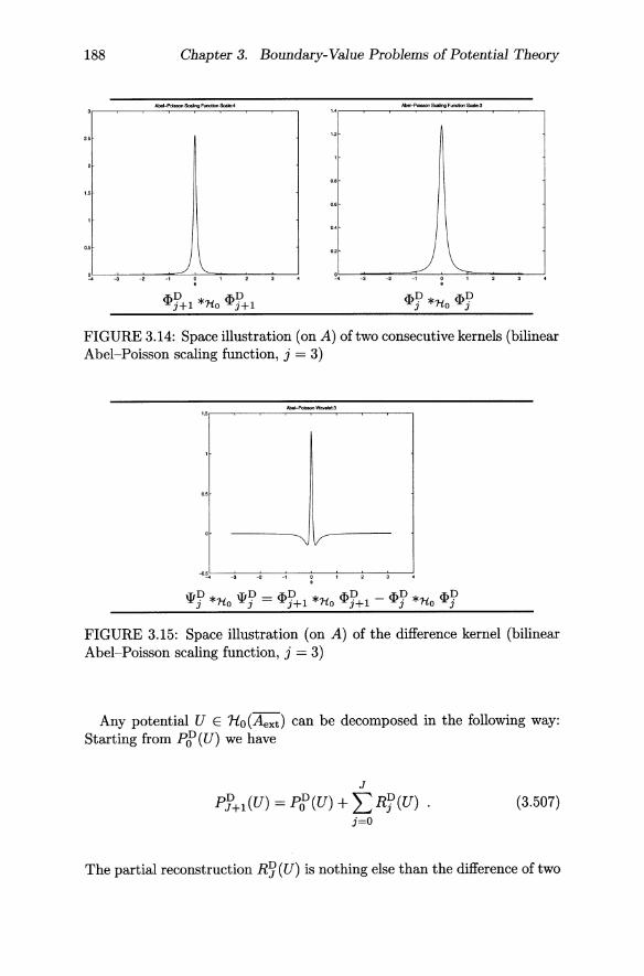
188 Chapter 3. Boundary-Value Problems of Potential Theory
AbeI-PoIssonScaHngFunctionScal8".
FIGURE 3.14: Space illustration (on A) oftwo consecutive kernels (bilinear Abel-Poisson scaling function, j = 3)
.T,D .T,D _ ",D ",D ",D ",D '¥j *'Ho '¥j - 'l"j+l *'Ho 'l"j+l - 'l"j *'Ho'l"j
FIGURE 3.15: Space illustration (on A) of the difference kernel (bilinear Abel-Poisson scaling function, j = 3)
Any potential U E 1to(Aext) can be decomposed in the following way: Starting from pf (U) we have
J
P'?+l(U) = pf(U) + LR~(U) (3.507) j=O
The partial reconstruction R~ (U) is nothing else than the difference oftwo

3.5. Runge-Walsh Approximation by Wavelet Expansion 189
AbaI_POlsson$cBl,ngFunctionSymbololScaIe4 AtJej-P<lissonSca,ng Function Symbol ofScale3
"
FIGURE 3.16: (Frequency) illustration of two consecutive symbols (bilinear Abel-Poisson scaling function, j = 3)
Abel-Poisson Wavelet Symbol of Scale3
FIGURE 3.17: (Frequency) illustration of the difference symbols (bilinear Abel-Poisson scaling function, j = 3)
"smoothings" P.?+l (U) and P.?(U) at consecutive scales
(3.508)
Moreover, in spectral language we have
(3.509)
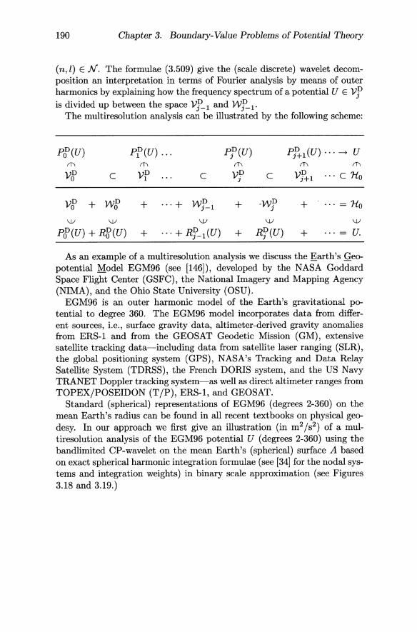
190 Chapter 3. Boundary-Value Problems of Potential Theory
(n, l) EN. The formulae (3.509) give the (scale discrete) wavelet decomposition an interpretation in terms of Fourier analysis by means of outer harmonics by explaining how the frequency spectrum of a potential U E Vf is divided up between the space Vf-l and Wf-l.
The multiresolution analysis can be illustrated by the following scheme:
Ptf>(U) PP(U) ... PP(U) P}?t-l (U) ... -+ U ffi ffi ffi ffi ffi
vtf> C Vp C VD J C Vf+1 ... c 110
Ve? + We? + ... + wD 1 J- + _WD J + ... = 110
'-lJ '-lJ '-lJ '-lJ '-lJ
Ptf>(U) + Rg(U) + ... + R~_l(U) + R~(U) + ... = U.
As an example of a multiresolution analysis we discuss the Earth's Geopotential Model EGM96 (see [146]), developed by the NASA Goddard Space Flight Center (GSFC), the National Imagery and Mapping Agency (NIMA), and the Ohio State University (OSU).
EGM96 is an outer harmonic model of the Earth's gravitational potential to degree 360. The EGM96 model incorporates data from different sources, i.e., surface gravity data, altimeter-derived gravity anomalies from ERS-1 and from the GEOSAT Geodetic Mission (GM), extensive satellite tracking data-including data from satellite laser ranging (SLR), the global positioning system (GPS), NASA's Tracking and Data Relay Satellite System (TDRSS), the French DORIS system, and the US Navy TRANET Doppler tracking system-as well as direct altimeter ranges from TOPEX/POSEIDON (TIP), ERS-1, and GEOSAT.
Standard (spherical) representations of EGM96 (degrees 2-360) on the mean Earth's radius can be found in all recent textbooks on physical geodesy. In our approach we first give an illustration (in m2/s2) of a multiresolution analysis of the EGM96 potential U (degrees 2-360) using the bandlimited CP-wavelet on the mean Earth's (spherical) surface A based on exact spherical harmonic integration formulae (see [34] for the nodal systems and integration weights) in binary scale approximation (see Figures 3.18 and 3.19.)
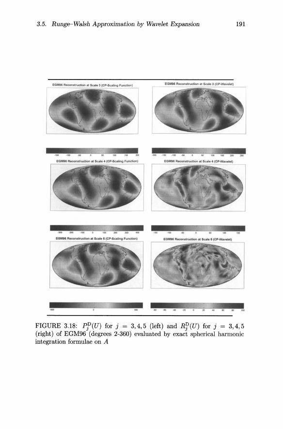
3.5. Runge-Walsh Approximation by Wavelet Expansion 191
·'00 .... IOKIO ... __
.... ... , ..
- - ... ... • • • lOCI
FIGURE 3.18: PF (U) for j = 3,4,5 (left) and R~ (U) for j = 3,4, 5 (right) of EGM96 (degrees 2-360) evaluated by exact spherical harmonic integration formulae on A
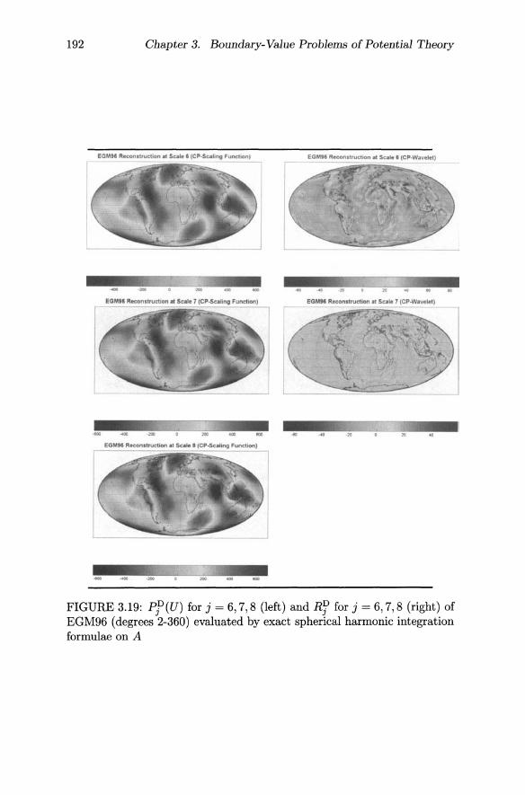
192 Chapter 3. Boundary-Value Problems of Potential Theory
EGMH R:ec:on:l'tJuaJon •• SeaJ •• (CP..seahr.g Fu.oclton)
.... .",
~ ... -.-.-'....-.'-' EGMM Re<:on.lrueUon It Sut. 7 (CP~Wavf:let)
l - .,., ". ... .. " ..
eOM" R:eeonltrUC1lon at Sea ... (CP.oSc.llling Function)
- ....
FIGURE 3.19: pF(U) for j = 6,7,8 (left) and R~ for j = 6,7,8 (right) of EGM96 (degrees 2-360) evaluated by exact spherical harmonic integration formulae on A

3.5. Runge-Walsh Approximation by Wavelet Expansion 193
30'
o·
30'
·8000 ·6000 ·4000 ·2000 o 2000 4000 6000
m
FIGURE 3.20: The (actual) Earth's surface ~ given by the TerrainBase data model of the National Geodetic Data Center in Boulder, Colorado
In what follows we give a multiresolution analysis of the EGM96 potential U (degrees 6~180) on the actual topography ~ of the Earth given by the TerrainBase data set of the National Geodetic Data Center in Boulder, Colorado (see Figure 3.20). The multiresolution analysis (see also [119]) is presented in Figure 3.21 - 3.24.
... ... ... ..
FIGURE 3.21: PF(U) for j = 3 (left) and Rf(U) for j = 3 (right) of EGM96 (degrees 6-180) on the TerrainBase data model of the Earth ~ using Abel~Poisson wavelets
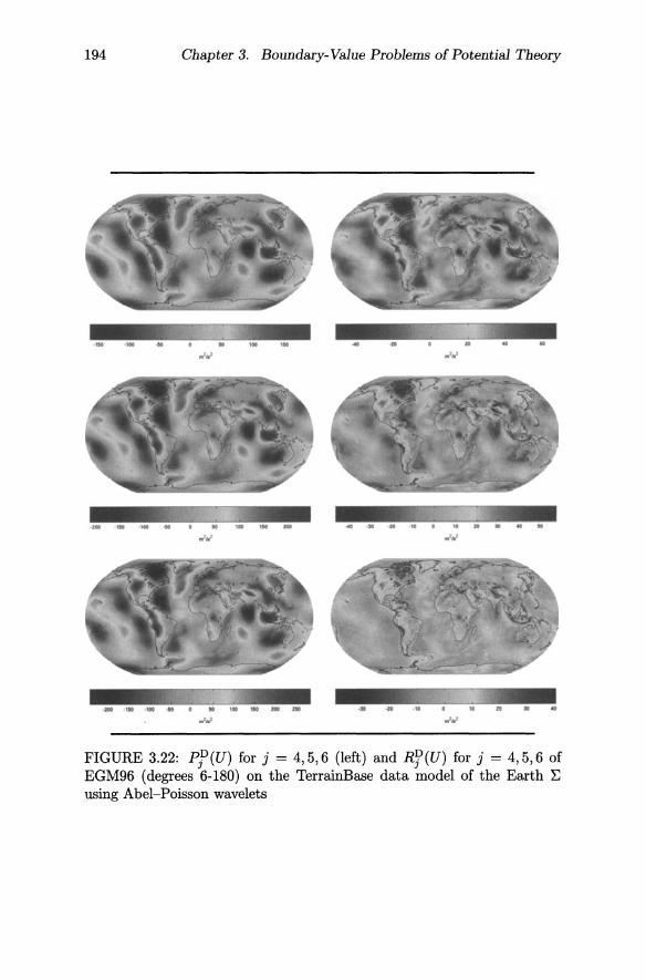
194 Chapter 3. Boundary-Value Problems of Potential Theory
1M .. .. II .. .11 .. • ..
• ~ ~ M • .. • • • •
It It • •
FIGURE 3.22: Pf (U) for j = 4,5,6 (left) and R~ (U) for j = 4,5,6 of EGM96 (degrees 6-180) on the TerrainBase data model of the Earth I; using Abel-Poisson wavelets

3.5. Runge-Walsh Approximation by Wavelet Expansion 195
.. .. • N • M • I • M • " •
'" .. , . '. ... - .. .. "
FIGURE 3.23: pF(U) for j = 7,8,9 (left) and R~(U) for j = 7,8,9 of EGM96 (degrees 6-180) on the TerrainBase data model of the Earth 2: using Abel-Poisson wavelets
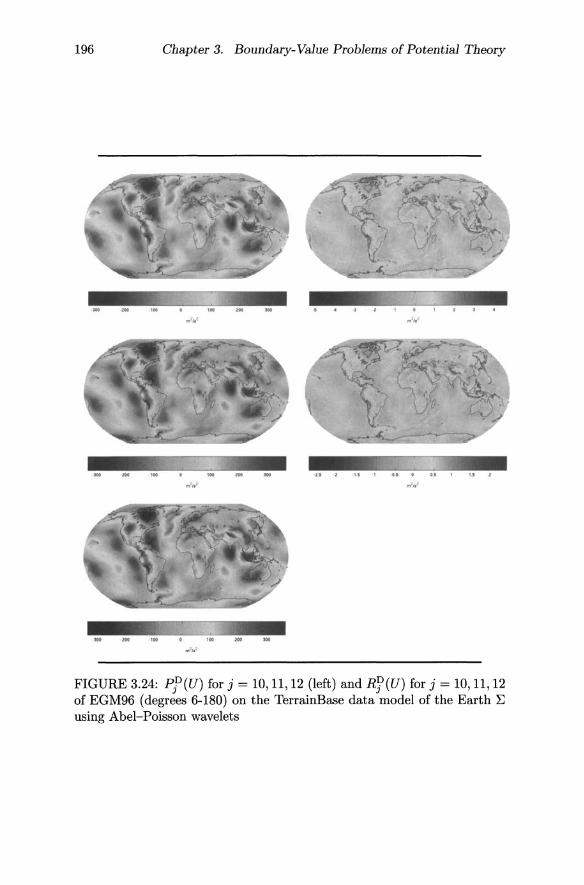
196 Chapter 3. Boundary-Value Problems of Potential Theory
U I " 1 .fa • .. till
.. ftII ,,, I" ,.. ..
FIGURE 3.24: P'P(U) for j = 10,11,12 (left) and R~(U) for j = 10,11,12 of EGM96 (degrees 6-180) on the TerrainBase data model of the Earth ~ using Abel-Poisson wavelets
3.5. Runge-Walsh Approximation by Wavelet Expansion 197
3.5.6 Least-Squares Approximation
The reconstruction formula (Theorem 3.32) may be rewritten as follows:
lim I!U - UJII H (X-) = 0, U E 1-lo(Aext), J---+oo 0 ext
(3.510)
where the J-Ievel scale discrete wavelet approximation now reads in shorthand notation as follows:
J
UJ = L 1 (WT)D(U)(j; y)w~y(-) dw(y) . j=-oo A
(3.511)
As in the continuous case we can make use of the projection property in the scale discrete case. We know already that (WT)D is a mapping from 1-lo(Aext) to 1-l(Z x Aext ), i.e.,
D --- ---(WT) : 1-lo(Aexd -+ 1-l(Z x Aext ),
where 1-l(Z x Aext) is the space of all functions U:(j;x) ~ U(j;x) with U(j;·) E 1-lo(Aext) for every j E Z and
f 1!U(j; ·)II~o(Aext) = f 1 (U(j; x))2 dw(x) < 00
j=-oo j=-oo A
(3.512)
It is not hard to see that
(3.513)
Hence, we are able to define the projection operator pD : 1-l(Z x Aexd -+
W D by
pD(U)(j'; y') = f 1 KD(j'; y' I j; y)U(j; y) dw(y), (3.514) j=-oo A
where
KD(j';y' I j;y) = i W~;yl(X)W~y(x) dw(x) = (W~;yl(.)' W~y(-))Ho(Aext) (3.515)
In similarity to results of the scale continuous case it can be deduced that pD is a projection operator. Therefore, we have the following characterization of W D .
LEMMA 3.22 U(·,·) E WD if and only if the "consistency condition"
U(j'; y') = f 1 KD (j'; y' I j; y) U(j; y) dw(y) j=-oo A
(3.516)
198 Chapter 3. Boundary-Value Problems of Potential Theory
00
L (KD(j'; y' I j; .), U(j; '))Ho(Aext) j=-oo
is satisfied.
Summarizing our results we obtain the following theorem.
Theorem 3.33 Let H be an arbitrary element of 1t(Z x Aext ). Then the unique function uJi E 1to(Aext) satisfying the property
II H(-,.) - tiJi(., ·)11 _ = inf_IIH(.,.) - tiD(., ·)11 -H(ZxAext ) UEHo(Aext) H(ZxAextl
(with tiD = (WT)D(U)) is given by
uJi(x) = f 1 U(j; y)lJ!~y(X) dw(y). j=-oo A
Moreover, we have the following theorem.
Theorem 3.34 For arbitrary U E 1to(Aext} the function ti = (WT)D(U) E WD is the unique element in 1t(Z x Aext) satisfying
3.5.7 Examples
Now we are prepared to introduce some important examples of scaling functions and corresponding wavelets (see [64]). We distinguish two types of wavelets: non-bandlimited and bandlimited wavelets. Since there are only a few conditions for a function to be a generator of a scaling function, a large number of wavelet examples may be listed. For brevity, however, we have to concentrate on a few examples.
3.5.7.1 Non-bandlimited Wavelets
All wavelets discussed in this subsection share the fact that their generators have a global support. Rational Wavelets: Rational wavelets are realized by the function <PI : [0, 00) -t IR given by
<PI(t) = (1 +t)-S, t E [0,00). (3.517)
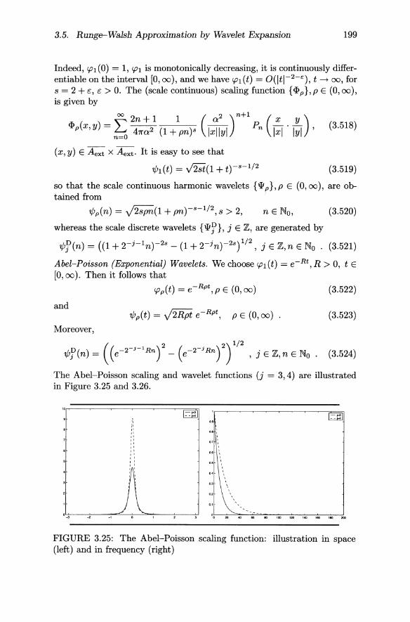
3.5. Runge-Walsh Approximation by Wavelet Expansion 199
Indeed, 'PI (0) = 1, 'PI is monotonically decreasing, it is continuously differentiable on the interval [0,00), and we have 'PI(t) = O(iti-2-e:), t ---- 00, for s = 2 + e, e > 0. The (scale continuous) scaling function {<pp}, p E (0,00), is given by
00 2n + 1 1 (a2 ) n+ I (x y) <pp(x, y) = ~ 47ra2 (1 + pn)s ixiiyi Pn j;I. TYT ' (3.518)
( x, y) E Aext x A ext . It is easy to see that
'l/JI(t) = V2St(1 + t)-S-I/2 (3.519)
so that the scale continuous harmonic wavelets {\]I p}, p E (0,00), are obtained from
'lj;p(n) = V2spn(1 + pn)-S-I/2, s > 2, n E No, (3.520)
whereas the scale discrete wavelets {\]I~}, j E IE, are generated by
'Ij;~(n) = ((1 + Ti- In )-2s - (1 + Tin )-2S)I/2, j E lE,n E No . (3.521)
Abel-Poisson (Exponential) Wavelets. We choose 'PI(t) = e-Rt,R > 0, t E [0,00). Then it follows that
'Pp(t) = e-Rpt , p E (0,00) (3.522)
and 'lj;p(t) = V2Rpt e-Rpt , p E (0,00) (3.523)
Moreover,
, j E lE,n E No . (3.524)
The Abel-Poisson scaling and wavelet functions (j = 3,4) are illustrated in Figure 3.25 and 3.26.
0.8 \
0.7 \
'-3 ClO 20 4() 60 80
FIGURE 3.25: The Abel-Poisson scaling function: illustration in space (left) and in frequency (right)

200 Chapter 3. Boundary-Value Problems of Potential Theory
1--------...)) \\~----___1
FIGURE 3.26: The Abel-Poisson wavelet function: illustration in space (left) and in frequency (right)
3.5.7.2 Bandlimited Wavelets
All wavelets discussed in this subsection are chosen in such a way that the support of their generators is compact. As a consequence the resulting wavelets are bandlimited. A particular result is that the Shannon wavelets provide us with an orthogonal multiresolution. Shannon Wavelet. The generator of the Shannon scaling function is defined by
<Pl(t) = {I, t E [0,1) 0, tE[l,oo).
(3.525)
The scale continuous harmonic scaling function {<I>p},p E (0,00), is given via
(3.526)
A scale continuous wavelet does not make sense. However, a scale discrete wavelet {wf}, j E Z, is available. More precisely,
Dn _{I, nE[2 j ,2H1 ) '¢j ( ) - 0, elsewhere. (3.527)
But this means that the scale discrete multiresolution is orthogonal (Le., VP+1 = Vp EB Wp is an orthogonal sum for all j).

3.5. Runge-Walsh Approximation by Wavelet Expansion 201
The Shannon scaling (j = 2,3,4) and wavelet functions (j = 2,3) are illustrated in Figures 3.27 and 3.28.
I~-1--3----
FIGURE 3.27: The Shannon scaling function: illustration in space (left) and in frequency (right)
1\
FIGURE 3.28: The Shannon wavelet function: illustration in space (left) and in frequency (right)
Cubic Polynomial Wavelet (CP-Wavelet). In order to have a higher intensity of the smoothing effect than in the case of Shannon wavelets we introduce a function 'PI : [0, (0) --> ~ in such a way that 'PII[O, 1] coincides with the uniquely determined cubic polynomial p : [0,1] --> [0,1] with the properties:
p(O) = 1 ,p(1) = 0,
p'(O) = 0, p'(1) = 0
It is easy to see that these properties are fulfilled by
p(t) = (1- t)2(1 + 2t), t E [0,1]
(3.528)
(3.529)
(3.530)
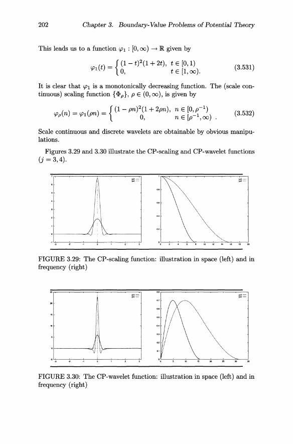
202 Chapter 3. Boundary-Value Problems of Potential Theory
This leads us to a function 'Pl : [0, 00) -t ~ given by
'Pl(t) = {(1 - t)2(1 + 2t), t E [0,1) 0, tE[l,oo).
(3.531)
It is clear that 'Pl is a monotonically decreasing function. The (scale continuous) scaling function {<I>p}, P E (0,00), is given by
(n) = (n) = { (1 - pn)2(1 + 2pn), n E [0, p-l) 'Pp 'Pl P 0, nE [p-l,oo) . (3.532)
Scale continuous and discrete wavelets are obtainable by obvious manipulations.
Figures 3.29 and 3.30 illustrate the CP-scaling and CP-wavelet functions (j = 3,4).
F'-~----
FIGURE 3.29: The CP-scaling function: illustration in space (left) and in frequency (right)
I:l=
FIGURE 3.30: The CP-wavelet function: illustration in space (left) and in frequency (right)
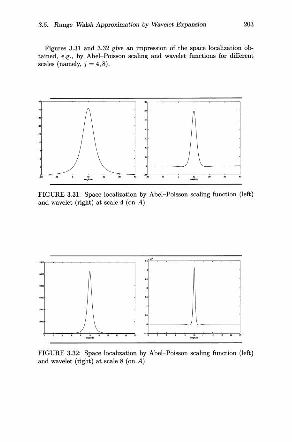
3.5. Runge-Walsh Approximation by Wavelet Expansion 203
Figures 3.31 and 3.32 give an impression of the space localization obtained, e.g., by Abel-Poisson scaling and wavelet functions for different scales (namely, j = 4,8).
" -"""
-~20~-----:7--~-----:,:::-, --=---=-----!. ........
FIGURE 3.31: Space localization by Abel-Poisson scaling function (left) and wavelet (right) at scale 4 (on A)
FIGURE 3.32: Space localization by Abel-Poisson scaling function (left) and wavelet (right) at scale 8 (on A)

204 Chapter 3. Boundary-Value Problems of Potential Theory
Next (see Figure 3.33) we present an illustration of a local multiresolution analysis using (exponential) non-bandlimited wavelets for a local EGM96 model (in m2s-2).
+
scale reconstruction at scale 6 wavelet reconstruction at scale 6
+ I •• + j"
wavelet reconstruction at scale 7 wavelet reconstruction at scale 8
scale reconstruction at scale 9
FIGURE 3.33: Local multiresolution analysis (j = 6, ... ,9) by exponential wavelets for the EGM96 model (degrees 2-360)

3.5. Runge-Walsh Approximation by Wavelet Expansion 205
Figure 3.34 shows a local multiresolution analysis by (exponential) nonbandlimited wavelets of the EGM96 model artificially disturbed by a buried mass point in the Pacific Ocean (close to the coast line of Chile). The disturbance is clearly seen in the wavelet reconstruction at scale 8 (see also [85]).
+
scale reconstruction at scale 7 wavelet reconstruction at scale 7
.. _-+
wavelet reconstruction at scale 8
scale reconstruction at scale 9
FIGURE 3.34: Local multiresolution analysis (j = 7,8,9) by exponential wavelets of EGM96 model (degrees 2-360) with an artificial disturbance
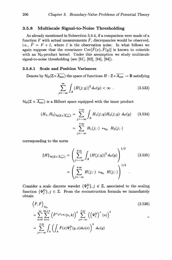
206 Chapter 3. Boundary-Value Problems of Potential Theory
3.5.8 Multiscale Signal-to-Noise Thresholding
As already mentioned in Subsection 3.4.4, if a comparison were made of a function F with actual measurements F, discrepancies would be observed, i.e., F = F + E, where E is the observation noise. In what follows we again suppose that the covariance Cov[F(x),F(y)] is known to coincide with an 1io-product kernel. Under this assumption we study multiscale signal-to-noise thresholding (see [81], [82], [84], [94]).
3.5.8.1 Scale and Position Variances
Denote by 1io (Z x Aext) the space of functions H : Z x Aext ---+ lR. satisfying
f 1 (H(j;y))2 dw(y) < 00 .
j=-oo A
(3.533)
1io(Z x Aext) is a Hilbert space equipped with the inner product
+00
(HI, H2 h£('L x Aext) = L 1 HI(j; y)H2(j; y) dw(y) j=-oo A
(3.534)
+00 L HI(j;') *'Ho H 2 (j;')
j=-oo
corresponding to the norm
(3.535)
Consider a scale discrete wavelet {'l1~},j E Z, associated to the scaling function {cI>~}, j E Z. From the reconstruction formula we immediately obtain
(3.536)
+00 ( )2 = i'fooL L F(x)lJ!~(y,x)dw(x) dw(y)

3.5. Runge-Walsh Approximation by Wavelet Expansion 207
+= = L 11 F(x)W~(Y,x) dw(x) 1 F(z)W~(Y,z) dw(z) dw(y) j=_= A A A
= jJ;=[ ([[ F(x)F(z)w~(X,y)W~(Z,y) dw(x) dw(Z)) dw(y)
= jJ;oo [[ F(x)F(z) (W~ *1to Wn (x, Z) dw(x) dw(z).
(3.537)
The signal scale and space variance of P at position yEn and scale j E Z is defined by
Varj;y (p) = i i p(x)p(z)\[J~(x, y)\[J~(z, y) dw(x) dw(z)
= (( \[J~ *1io P) (y)) 2 . (3.538)
The signal scale variance of P is defined by
(3.539)
Obviously, we have for the "total variance" of P E ?to
2 +00
IIPII1io(Aextl = . L Varj (p) J=-OO
+00
= jJ;oo l Varj;y (P) dw(y) (3.540)
= II (Var.;. (p))1/2112 _ 1iO(ZxAext)
Expressed in the spectral language of spherical harmonics we get
This shows us that
(3.542)
Figures 3.35 and 3.36 show examples of CP-wavelet variances for EGM96 (degrees 2-360). More detailed information can be found in [43].

208 Chapter 3. Boundary-Value Problems of Potential Theory
o 2000 4000 6000
FIGURE 3.35: CP-wavelet variances for scale 6 of EGM96 [m4 /s4]
o 2000 4000 6000 8000 10000
FIGURE 3.36: CP-wavelet variances for scale 7 of EGM96 [m4 /s4 ]

3.5. Runge-Walsh Approximation by Wavelet Expansion 209
3.5.8.2 Scale Covariances
Suppose that K : (x, y) ~ K(x, y), (x, y) E Aext x Aext' is an Ho-product kernel given by (3.291). The error theory is based on the scale and space error covariance at y E Aext'
Covj;y(K) = ii K(x, z)wf(x, y)wf(z, y) dw(x) dw(z), Y E Aext
(3.543) The scale error covariance is defined by
(3.544)
We obviously have in spectral language
(3.545)
3.5.8.3 Scale and Space Estimation
The signal and noise scale "intersect" at the scale and space resolution set Zres with
Zres C Z = {(j;y) Ij E Z,y E Aext}
We distinguish the following cases:
(i) Signal dominates noise
Varj;y (p) 2: Covj;y(K), (j; y) E Zres .
(ii) Noise dominates signal
Varj;y (P) < Covj;y(K), (j; y) ~ Zres .
(3.546)
(3.547)
(3.548)
3.5.9 Wavelet Representation of Functions on Regular Surfaces
Suppose that there is given a continuous function on a regular surface from which function values are available on a finite set of discrete points on ~. Then, an extended version of Helly's theorem (see [222]) shows that, corresponding to this continuous function on ~, there exists a member F of class Ho(Aext) in an (c/2)-neighborhood that is consistent with the function values of the continuous function on ~ for the known finite set of discrete points. Moreover, this function F of class Ho(Aext) may be assumed to be in (c/2)-accuracy to a member Fo, ... ,m of class Harmo, ... ,m(~) which can

210 Chapter 3. Boundary-Value Problems of Potential Theory
be supposed to be consistent with the known function values as well. In other words, corresponding to any continuous function on a regular surface ~, there exists in €-accuracy a bandlimited function Fo, ... ,m such that this bandlimited function Fo, ... ,m coincides at all given points with the function values of the original continuous function on the regular surface~. This is the reason why we are interested in wavelet approximations of functions Fo, ... ,m of class Harmo, ... ,m(~) from discretely given function values.
To be more concrete, let us assume that there exists an integer m ~ 0 and a potential UO, ... ,m E Harmo, ... ,m(Aext) such that UO, ... ,ml~ is just equal to the function Fo, ... ,m we are looking for. Furthermore, let us restrict ourselves to compactly supported generators 'P~, 'ljJ~, defining a sequence (mj )j=O,l, ... with
m · - 2j +1 - 1 J' 0 1 J - ,= , , ... (3.549)
such that
(3.550)
and (3.551)
Our strategy is to represent UO, ... ,m E Harmo, ... ,m(Aext) by a J-Ievel wavelet approximation (UO, ... ,m)J with J chosen in such a way that mJ ~ m. The restriction (Fo, ... ,rn)J = (UO, ... ,rn)JI~ then serves as a uniform approximation to F E 1tO(Aext)l~ on the regular surface ~ (note that, in particular, (FO, ... ,mh agrees with Fo, ... ,m uniformly on ~ in the case of Shannon wavelets).
We want to present three algorithms (see [100]) on how to obtain (FO, ... ,mh from discretely given data of Fo, ... ,m on ~ using wavelet decomposition and reconstruction. In all three cases we use for reconstruction purposes the fact that, because of (3.550) and (3.551), both (U(y), <I>~y(-)hio and
D ---(WT) (U)(j;·) are of class Harmo, ... ,mj(Aext).
3.5.9.1 First Wavelet Variant
Using the first variant of outer harmonic exact integration (Lemma 3.9) developed in Subsection 3.4.5.1 we obtain a first formulation of a fully discrete wavelet representation of a function on a regular surface.
Theorem 3.35 Suppose that X~ = {x~j, ... ,x~j} C~, with
J J
m+mj M j = L (r + 1)2, j = 0, ... , J, (3.552)
r=O
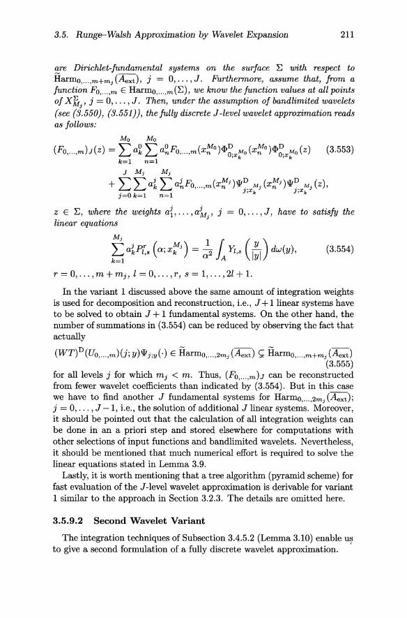
3.5. Runge-Walsh Approximation by Wavelet Expansion 211
are Dirichlet-fundamental systems on the surface E with respect to Harmo, ... ,m+mj (Aext ), j = 0, ... , J. Furthermore, assume that, from a function Fo, ... ,m E Harmo, ... ,m(E), we know the function values at all points of xft-. , j = 0, ... ,J. Then, under the assumption of band limited wavelets
J
(see (3.550), (3.551)), the fully discrete J-level wavelet approximation reads as follows:
Mo Mo
(Fo, ... ,m)J(z) = Lag L a~Fo, ... ,m(x~O)<p~x~o (x~O)<p~x~o (z) k=l n=l
(3.553)
J Mj M j
+ LLaiLa~Fo, ... ,m(x~j)w~ Mj(X~j)W~ Mj(Z), j=O k=l n=l J'X k J'X k
Z E E, where the weights a{, ... , air., j = 0, ... , J, have to satisfy the J
linear equations
M·
~aiP!,s (a;x~j) = ~2l Yz,s C~I) rM(y), (3.554)
r = 0, ... , m + mj, l = 0, ... , r, s = 1, ... , 2l + l. In the variant 1 discussed above the same amount of integration weights
is used for decomposition and reconstruction, i.e., J + 1 linear systems have to be solved to obtain J + 1 fundamental systems. On the other hand, the number of summations in (3.554) can be reduced by observing the fact that actually
D . - -- - --(WT) (UO, ... ,m)(J; y)Wj;y(') E Harmo, ... ,2mj (Aext) s:;; Harmo, ... ,m+mj (Aext)
(3.555) for all levels j for which mj < m. Thus, (Fo, ... ,m)J can be reconstructed from fewer wavelet coefficients than indicated by (3.554). But in this case we have to find another J fundamental systems for Harmo, ... ,2mj (Aext); j = 0, ... ,J -1, i.e., the solution of additional J linear systems. Moreover, it should be pointed out that the calculation of all integration weights can be done in an a priori step and stored elsewhere for computations with other selections of input functions and bandlimited wavelets. Nevertheless, it should be mentioned that much numerical effort is required to solve the linear equations stated in Lemma 3.9.
Lastly, it is worth mentioning that a tree algorithm (pyramid scheme) for fast evaluation of the J-Ievel wavelet approximation is derivable for variant 1 similar to the approach in Section 3.2.3. The details are omitted here.
3.5.9.2 Second Wavelet Variant
The integration techniques of Subsection 3.4.5.2 (Lemma 3.10) enable us to give a second formulation of a fully discrete wavelet approximation. I
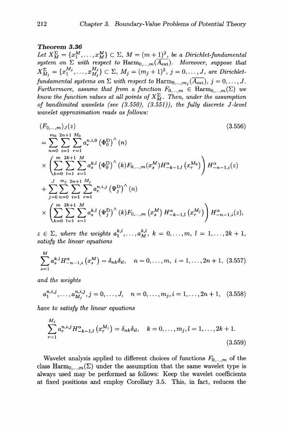
212 Chapter 3. Boundary-Value Problems of Potential Theory
Theorem 3.36 Let XB- = {xr, ... ,x~n c E, M = (m + 1)2, be a Dirichlet-fundamental system on E with respect to Harmo, ... ,m(Aext). Moreover, suppose that
X~ = {x~j, ... , x~j} c E, M j = (mj + 1)2, j = 0, ... , J, are Dirichlet-J J
fundamental systems on E with respect to Harmo, ... ,mj (Aexd, j = 0, ... , J. Furthermore, assume that from a function FO, ... ,m E Harmo, ... ,m(E) we know the function values at all points of X~. Then, under the assumption of band limited wavelets (see (3.550), (3.551)), the fully discrete J -level wavelet approximation reads as follows:
(3.556)
n=O i=1 r=1
x (~2~1 t. a~,l (<I>~)t\ (k)Fo, ... ,m(x~)H'=k_1,1 (x~O)) H'=n_1,i(Z)
J mj 2n+1 Mj
+ LL L La~,i,j (\IJ~)'" (n) j=O n=O i=1 r=l
x (~2~1 t. a~,l (\IJ~)'" (k)Fo, ... ,m (x~) H'=k-l,l (x~j)) H'=n-l,i(Z),
"" h th . ht k,l k,l k ° l 1 2k 1 Z E u, were e wezg s a1 , ... ,aM , = , ... ,m, = , ... , +, satisfy the linear equations
M
""' k,IHO! ( M) _ J: J:. ~ as -n-l,i X 8 - unku.l, n = 0, ... ,m, i = 1, ... ,2n + 1, (3.557) 8=1
and the weights
n,i,j n,i,j· - ° J a l , ... , aM· ,J - , ... , , J
n = 0, ... , mj, i = 1, ... , 2n + 1, (3.558)
have to satisfy the linear equations
Mj ""' an,i,jHO! (xMj) J: J: ~ r -k-l,l r = UnkUil, k = 0, ... , mj, l = 1, ... , 2k + 1. r=l
(3.559)
Wavelet analysis applied to different choices of functions FO, ... ,m of the class Harmo, ... ,m(E) under the assumption that the same wavelet type is always used may be performed as follows: Keep the wavelet coefficients at fixed positions and employ Corollary 3.5. This, in fact, reduces the
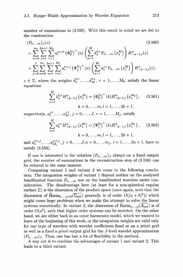
3.5. Runge-Walsh Approximation by Wavelet Expansion 213
number of summations in (3.556). With this result in mind we are led to the construction
(3.560)
= ~ ~ ~ an,i,O (g,D)" (n) ~ (i0,r F. (XM) HC> .(z) mo 2n+1 Mo ( M ) ~ L...t L....t r 0 L....t s O, ... ,m s -n-l,z n=O i=l r=l 8=1
J mj 2n+1 Mj ( M ) + ~~ ~ ~a~'i,j (W~)" (n) ~a~,rFO, ... ,m (X~) H':n-1,i(Z),
" h th . ht -O,r -O,r 1 .,.,. . fy h l' z E L;, were e WeIg s a1 , ... , aM' r = , ... , 1V10, satls t e lnear equations
M
L (i~,r H~\-l,1 (x~) = (g,~)" (k)H':k-1,1 (x~o) , (3.561) 8=1
k = 0, ... , m, l = 1, ... , 2k + 1,
t · 1 j,r j,r. - 0 J - 1 M t' fy respec lve y, a1 , ... , aM' J - , ... , , r - , ... , j, sa IS
M
L a~,r H':k-1,1 (x~) = (w~)" (k)H':k-1,l (x~j) , (3.562) 8=1
k = 0, ... , m, 1= 1, ... , 2k + 1,
d n,i,j n,i,j. - 0 J - 0 . - 1 2 + 1 h t an a1 , ... , a Mj , J - , ... , , n - , ... , mj, 2 - , •.. , n , ave 0
satisfy (3.559).
If one is interested in the solution (Fo, ... ,m)J always on a fixed output grid, the number of summations in the reconstruction step of (3.556) can be reduced in the same manner.
Comparing variant 1 and variant 2 we come to the following conclusion: The integration weights of variant 1 depend neither on the analyzed bandlimited function FO, ... ,m nor on the bandlimited wavelets under consideration. The disadvantage here (at least for a non-spherical regular surface ~) is the dimension of the product space (once again, note that the
dimension of Harmo, ... ,a+b(~ext) generally is of order O((a + b)3)) which might cause huge problems when we make the attempt to solve the linear systems numerically. In variant 2, the dimension of Harmo, ... ,a(Aexd is of order O(a2 ), such that higher order systems can be inverted. On the other hand, we are either back in an outer harmonics model, which we wanted to leave at the beginning of this work, or the integration weights are valid only for one type of wavelets with wavelet coefficients fixed at an a priori grid as well as a fixed a priori output grid for the J-level wavelet approximation (Fo, ... ,m)J. Thus, one has lost a lot of flexibility in the method.
A way out is to combine the advantages of variant 1 and variant 2. This leads to a third variant.
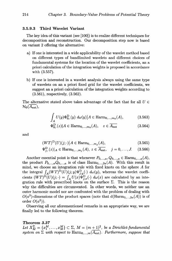
214 Chapter 3. Boundary-Value Problems of Potential Theory
3.5.9.3 Third Wavelet Variant
The key idea ofthis variant (see [100]) is to realize different techniques for decomposition and reconstruction. Our decomposition step now is based on variant 2 offering the alternative:
a) If one is interested in a wide applicability of the wavelet method based on different types of bandlimited wavelets and different choices of fundamental systems for the location of the wavelet coefficients, an a priori calculation of the integration weights is proposed in accordance with (3.557).
b) If one is interested in a wavelet analysis always using the same type of wavelets on an a priori fixed grid for the wavelet coefficients, we suggest an a priori calculation of the integration weights according to (3.561), respectively, (3.562).
The alternative stated above takes advantage of the fact that for all U E
Ho(Aext),
and
i U(y)<P~.(y) dw(y)IA E Harmo, ... ,mo(A),
<P~.(z)IA E Harmo, ... ,mo(A), z E Aext
(WT)D(U)(j; ')IA E Harmo, ... ,mj (A),
(3.563)
(3.564)
(3.565) D ---
wj;.(Z)IA E Harmo, ... ,mj(A), z E Aext, j = 0, ... , J. (3.566)
Another essential point is that whenever PO, ... ,a, QO, ... ,a E Harmo, ... ,a(A), the product PO, ... ,aQo, ... ,a is of class HarmO, ... ,2a(A). With this result in mind, we choose an integration rule with fixed knots on the sphere A for the integral fA(WT)D(U)(j;y)w~y(.) dw(y), whereas the wavelet coefficients (WT)D(U)(j;·) = fA U(x)w~x(-) dw(x) are calculated by an integration rule with prescribed knots on the surface:E. This is the reason why the difficulties are circumvented. In other words, we neither use an outer harmonic model nor are confronted with the problem of dealing with O(a3 )-dimensions of the product spaces (note that d(Harmo, ... ,2a(A)) is of order O(a2 )).
Observing all our aforementioned remarks in an appropriate way, we are finally led to the following theorem.
Theorem 3.37 Let xfr = {xr, ... , x~n c :E, M = (m + 1)2, be a Dirichlet-fundamental system on :E with respect to Harmo, ... ,m(Aext). Furthermore, suppose that
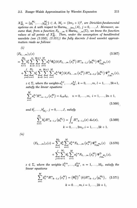
3.5. Runge-Walsh Approximation by Wavelet Expansion 215
x fI. = {y~j , ... , y~j} c A, M j = (2mj + 1)2, are Dirichlet-fundamental J J
systems on A with respect to Harmo, ... ,2mj (A), j = 0, ... , J. Moreover, as-sume that, from a function Fo, ... ,m E Harmo, ... ,m(~), we know the function values at all points of X1. Then, under the assumption of band limited wavelets (see (3.550), (3.551)) the fully discrete J-level wavelet approximation reads as follows:
(i)
(Fo, ... ,m)J(z) (3.567) Mo m 2k+1 M
= L b~ L L La~,I<I>~(k)Fo, ... ,m (x~) H~k_1,z(y~o) <I>~y~O (z) n=l k=O 1=1 8=1
J Mj m 2k+1 M
+ L Lot, L L La~,lwj(k)Fo, ... ,m (x~) H~k-1,1 (y~j) W~y:::,"j (z), J=O n=l k=O 1=1 8=1
(ii)
z E~, where the weights a~,l, ... ,a';j, k = 0, ... ,m, 1 = 1, ... , 2k+1, satisfy the linear equations
M
La~,IH~n_1,i (x~) = OnkOil, n = 0, ... , m, i = 1, ... , 2n + 1, 8=1
(3.568)
and b{, ... , llM' j = 0, ... , J, satisfy J
M· t ot,H~k-1,i (y~j) = J H~k_1,i(X) dw(x), n=l A
(3.569)
k = 0, ... , 2mj, i = 1, ... , 2k + 1.
Mo M
(Fo, ... ,m)J(z) = L b~ L a~,n Fo, ... ,m (x~) <I>~y~O (z) (3.570) n=l 8=1
J Mj M
+ L L ot, L a~,n Fo, ... ,m (x~) W~ M j (z), j=O n=l 8=1 J,yn
~ h th . ht -O,n -O,n 1 A". . ,I. h z E LJ, were e wezg s a1 , ... , aM , n = , ... , 1V10, satzsJy t e linear equations
M
L a~,n H~k-l,i (x~) = (<I>~)" (k)H~k_1,i (y~o), (3.571) 8=1
k = 0 ... , m, i = 1, ... , 2k + 1,
I

216 Chapter 3. Boundary-Value Problems of Potential Theory
and the weights a{,n, ... ,ak;', j = 0, ... ,J, n = 1, ... ,Mj , satisfy
M
La~,nH~k_1,i (x~) = (1}!~)1\ (k)H~k_1,i (y~j), (3.572) 8=1
k = 0, ... ,m, i = 1, ... ,2k + 1,
and b{, ... ,aiM' j = 0, ... ,J, satisfy {3.569}. J
The inspection of Theorem 3.37 leads us to the impression that a great number of linear systems must be solved. But if we look carefully we observe that we are always confronted with the same coefficient matrix. Having done the inversion once, all weights of the integration rules can be obtained by a matrix-vector multiplication and stored elsewhere for computations with other boundary values. In this respect it is also of interest to mention that the solution of the linear systems determining the weights of the reconstruction step (3.569) can be avoided completely. As a matter of fact, placing the knots of the integration rules determining the wavelet coefficients for each detail step j = 0, ... , J on a special longitudelatitude grid on the sphere A leads us to a set of integration weights for reconstruction purposes that is explicitly available (see, for example, [34] and [208] and the references therein).
3.5.10 Wavelet Modelling of Boundary-Value Problems
We are now interested in a fully discrete wavelet approximation seen from the point of view of potential theory. The keystone is that when using bandlimited wavelets, we do not need the wavelet transform at all positions. It suffices to know the wavelet transform on a finite set of linear functionals for each scale j. In conclusion, each J-Ievel wavelet approximation can be expressed exactly as a finite sum.
Our wavelet concept again is discussed under the following non-restrictive assumptions:
(i) The generator 'P~ [0, <Xl) ----+ lR of a scale discrete scaling function satisfies
supp 'P~ C [0,1].
(ii) The generator 'l/Jf] : [0, <Xl) ----+ lR of the mother wavelet satisfies
supp 'I/J~ C [0, 2].
Then it follows that
D j supp 'Pj C [0,2 ],
supp 'I/J~ C [0,2)+1].
(3.573)
(3.574)

3.5. Runge--Walsh Approximation by Wavelet Expansion 217
In other words, we restrict ourselves to the conditions (3.550) and (3.551). We recapitulate the essential ideas of the Runge-Walsh approach based
on bandlimited wavelets: Corresponding to a given potential V of the class Pot(O) (:Eext ), there exists in c-accuracy on :Eext a bandlimited potential in 'Ho(Aext), (namely UO, ... ,m E Harmo, ... ,m(Aext)) consistent with the original data (i.e., Vi = LiU = LiUO, ... ,m, i = 1, ... , M). This result, on which the (Runge--Walsh) Fourier theory of boundary-value problems has already been based in Section 3.4, is now the point of departure for Runge--Walsh approximations of potentials UO, ... ,m of class Harmo, ... ,m(:Eexd uniformly on :Eext from a finite set of functional values. To be more specific, our strategy is to represent UO, ... ,m E Harmo, ... ,m(Aext) by a J-level approximation (UO, ... ,m)J with J chosen in such a way that mJ ;::: m (note that UO, ... ,m coincides with (UO, ... ,m)J uniformly on :Eext in the case of Shannon wavelets). We want to express the J-level wavelet approximation (UO, ... ,m)J of UO, ... ,m(mJ ;::: m) exactly only by use of the M values V1, ... , VM corresponding to the linear functionals L 1 , ... , L M. To this end we again observe that J UO, ... ,m(y)<P~y(·)dw(y)IA E Harmo, ... ,mo(A),
A
(WT)D(Uo, ... ,m)(j; ')IA E Harmo, ... ,mj (A), j = 0, ... , J.
(3.575)
(3.576)
Moreover, we again use the fact that whenever F, G E Harmo, ... ,m(A), the product FG is of class HarmO, ... ,2m(A).
The results of Subsection 3.4.5.4 on exact outer harmonics integration formulae enable us to develop a constructive version of the Runge-Walsh theorem by means of a J-level wavelet approximation when the potential U we are looking for is assumed to be a member of class 'Ho (Aext) I Lext (note that 'HO(Aext)l:Eext is a uniformly dense subset of Pot (0) (:Eext )). Essential tools of our considerations are Lemma 3.12 and Lemma 3.13.
Theorem 3.38 Let {Lj'f, ... , L~}, M = (m + 1)2, be a Harmo, ... ,m-fundamental system as defined by (3. 347}. Furthermore, suppose that {y~j, . .. , y~j} C
J
A, M j = (2mj + 1)2, define Harmo, ... ,2mj-Dirichlet-fundamental systems on A, j = 0, ... , J. Moreover, assume that, from a potential UO, ... ,m E Harmo, ... ,m(Aext), there are known the data LIfuo, ... ,m = Vi, i = 1, ... , M. Then, under the assumption of bandlimited wavelets, the fully discrete Jlevel wavelet approximation (UO, ... ,m)J of UO, ... ,m reads as follows: (i)
(3.577) Mo m 2k+1 M
= L b~ L L L a~,1 (<p~)!\ (k)v 8 H'.:.k_1,1 (y~o) <P~y~o (z) n=l k=O 1=1 8=1

218 Chapter 3. Boundary-Value Problems of Potential Theory
J Mj m 2k+1 M
+ L L ll.. L L La~,l (w~t (k)v8H~k_1,1 (y~j) W~yMj (z), j=O n=l k=O 1=1 8=1 ' n
E ~ h th . ht k,l k,l k 0 l 1 2k + 1 z L.iext, were e wezg sal , ... ,aM , = , ... ,m, = , ... , , satisfy the linear equations
M
La~,I£~H~n_1,i(-) = OnkOil, (3.578) 8=1
n = 0, ... , m, i = 1, ... , 2n + 1 and b{, ... , liM" j = 0, ... , J satisfy the 1
linear equations
i = 1, ... ,Mj .
(ii)
M j
L ll..KHarmo, ... ,2"'j (Eext) (y~j , y~j ) n=l
= J KHarmo, ... ,2"'j (Eextl (y~j, x) dw(x), A
(UO, ... ,m)J(z)
(3.579)
(3.580)
z E Eext' where the weights ii~,n, ... ,iir;,;t, n = 1, ... ,Mo; satisfy the linear equations
M
""""' -O,n£M£MK _ ( ) _ £M ifo.D ~a8 i 8 Harmo, ... ,,,,(Eextl .,. - i '±'O;y;'!o, (3.581) 8=1
. 1 M d th 0 ht j,n j,n. - 0 J 1 M z = , ... , ,an e wezg s a1 , ... , aM' J - , ... , ,n = , ... , j,
satisfy
M
L j,n£M£MK - ( ) - £M .T,D a8 i 8 Harm (E) ',' - i 'l'. M j , O, ... ,Tn ext JOY 1 ' n 8=
(3.582)
i = 1, ... M, and b{, ... , liM' j = 0, ... , J, satisfy (3. 579}. 1
Once more it should be remarked that a great number of linear systems must be solved. But if we look carefully we realize that we are always confronted with the same coefficient matrix. Having inverted the coefficient
3.5. Runge-Walsh Approximation by Wavelet Expansion 219
matrix once, all weights for numerical integration can be obtained by a matrix-vector multiplication and stored elsewhere (in an a priori step for computation). In addition, it should be mentioned that the solution of the linear systems determining the weights of the reconstruction step (3.579) can be avoided completely if we place the knots for numerical integration of the wavelet coefficients for each detail step j = 0, ... , J on a special longitude-latitude grid on the sphere A. The corresponding set of integration weights for reconstruction purposes are explicitly available without solving any linear system (for more details the reader is referred to [34], [208]).
3.5.10.1 Exterior Dirichlet Problem
Assume that there is available from a function Fo, ... ,m E Harmo, ... ,m(~) a finite set of function values at certain discrete points on a regular surface ~. Our purpose is to solve the exterior Dirichlet problem U E Harmo, ... ,m(~ext), UO, ... ,ml~ = Fo, ... ,m using wavelet methods. For simplicity we restrict ourselves to the integration formulae of variant 3.
Theorem 3.39 Under the assumptions of Theorem 3.38 with L!t F = F(xr), i = 1, ... , M, the fully discrete J -level wavelet approximation of the solution of the exterior Dirichlet problem UO, ... ,m E Harmo, ... ,m(~ext), UO, ... ,ml~ = Fo, ... ,m reads as follows:
(i)
(3.583) Mo m 2k+1 M 1\
= Lb~L L La~,l (1)~) (k)Fo, ... ,m (x~) H':.k-1,1 (y~o) 1>o;y~o(z) n=l k=O 1=1 8=1
J M j m 2k+1 M 1\
+ L L Il.. L L L a~,l (Wn (k)FO, ... ,m (x~) H':.k-1,1 (y~j) Wj;y:;:j (Z), J=O n=l k=O 1=1 8=1
z E ~ext.
(ii)
Mo M
(UO, ... ,m)J(Z) = L b~ L a~,n Fo, ... ,m(X~)~O;Y~O (Z) (3.584) n=1 8=1
J Mj M
+ "" at, "a~,n FO, ... ,m(X~)W .. M j (Z), ~~ ~ l,Yn Z E ~ext.
j=O n=1 8=1

220 Chapter 3. Boundary-Value Problems of Potential Theory
The formulae (3.583) and (3.584) are especially valid for z E E, i.e., we automatically obtain a J-Ievel wavelet approximation of the boundary function Fo, ... ,m which is denoted by (Fo, ... ,m)J (by applying Shannon wavelets we already know that (Uo, ... ,mh = UO, ... ,m and, thus, (Fo, ... ,mh = Fo, ... ,m).
By treating non-bandlimited potentials U E Hs(Eext), s > 1, the developed integration formulae are only valid in an approximate sense. To be more concrete, if UJ denotes the J-Ievel wavelet approximation we actually calculate an approximation (UO, ... ,m)J by performing the numerical integration methods in (3.583) and (3.584). Since this approximation is also harmonic in Eext the maximal error between U J and its numerical approximation (UO, ... ,mh is attained at the boundary E. Thus, the numerical error can be estimated by virtue of Theorem 3.22.
3.5.10.2 Exterior Neumann Problem
Assume that there are available from a potential UO, ... ,m of the class Harmo, ... ,m(Eexd the (oblique) derivatives GO, ... ,m = aUt, ... ,m/a)..r, at a finite set of discrete points on a regular surface E. The intent is to solve the exterior Neumann problem UO, ... ,m E Harmo, ... ,m(Eext), aUt, ... ,m/a)..r, = GO, ... ,m.
As in the case of the Dirichlet problem we consider only variant 3 of Subsection 3.4.5.4. But, for the decomposition step we need in contrast to the Dirichlet problem an integration method in terms of (oblique) derivatives on E. To be more specific, if PO, ... ,a E Harmo, ... ,a(Eexd and Q E Ho(Aext), then an integration rule of type
r M oR J, PO, ... ,a(y)Q(y)dw(y) = L ar a~~,a (Xr),
A r=l
is required for our purposes. The construction proceeds as follows: We introduce Neumann-fundamental systems. Then we describe integration formulae in terms of (oblique) derivatives (Lemma 3.23). Finally, the fully discrete wavelet approximation is discussed.
Definition A set XEr = {xj'1, ... ,x~n c E, M = (a + 1)2, is called a )..-Neumann-fundamental system on E with respect to Harmo, ... ,a(Eexd if the matrix
(
{)~E H'.:l,l (xj'1) {)~E H'.:l,l (x~) )
{)~E H'.:a-~'2a+1 (xj'1) ... {)~E H'.:a-~'2a+l (x~) is regular.
This definition leads us to the formulation of the following lemma.
3.5. Rung~Walsh Approximation by Wavelet Expansion 221
LEMMA 3.23 LetX'fr = {x{W, ... ,x~:n C~, M = (a+1)2, be a Ar,-Neumann-fundamental system on ~ with respect to Harmo, ... ,a(~exd. Furthermore, suppose that PO, ... ,a E Harmo, ... ,a(~ext) and Q E 1io(Aext). Then we have
(i)
( a 2n+l M oF, I, PO, ... ,a(y)Q(y) dw(y) = L L La~,jQA(n,j) o~···,a (x~)
A n=Oj=l r=l r,
(3.585) t II . ht n,j n,j - ° . - 1 2 1 t' f . Jor a wezg sal , ... , aM , n - , ... , a, J - , ... , n+ ,sa zs. yzng
M
" n,j ~HQ ( M) - s: s:.. k k ~ ar OAr, -k-l,i xr - UnkUp, = 0, ... ,a, i = 1, ... ,2 + 1. r=l
(3.586)
(ii)
( M oF, JJ PO, ... ,a(y)Q(y) dw(y) = Lar o~~,a (x~)
A r=l
(3.587)
for all weights al, ... , aM satisfying
M
L ar o~r, H'.:'.k-l,i (x~) = QA(k, i), k = 0, ... , a, i = 1, ... , 2k + 1. r=l
(3.588)
The proof of Lemma 3.23 follows in analogy to conclusions given in Subsection 3.4.5.4.
Summarizing our results we therefore obtain a fully discrete wavelet approximation for the solution of the oblique exterior Neumann problem.
Theorem 3.40 LetX'fr = {x{W, ... ,x~n C~, M = (m+1)2, be a Ar,-Neumann-fundamental system on ~ with respect to Harmo, ... ,m(Aext). Furthermore, let xtr. =
J
{y~j , ... ,y~j} c A, M j = (2mj + I?, be Dirichlet-fundamental systems J
on A with respect to Harmo, ... ,2mj (A), j = 0, ... , J. Moreover, assume that,
from a function UO, ... ,m E Harmo, ... ,m(~ext), there are known the (oblique) derivatives GO, ... ,m = oUt, ... ,m/OAr, at all points of X'fr. Then, under the assumption of bandlimited wavelets (see (3.550), (3.551)) the fully discrete J -level wavelet approximation of the solution of the exterior Neumann prob-
(- + lem UO, ... ,m E Harmo, ... ,m ~exd, oUO, ... ,m/OAr, = GO, ... ,m reads as follows:
222
(i)
(ii)
Chapter 3. Boundary-Value Problems of Potential Theory
(UO, ... ,m)J(Z) (3.589) Mo
=I:b~ n=l
m 2k+1 M xI: I: I:a~,l (<T>~)"(k)Go, ... ,m (X~)H':k_1,1 (y~o)<T>~y~o(z)
k=O 1=1 8=1 J M j
+I:I:~ j=O n=l
m 2k+1 M x I: I: I:a~,l (W~)A(k)Go, ... ,m (x~) H':k-1,1 (y~j) W~y~j (z),
k=O 1=1 s=l
Z E ~ext' where the weights a~,l, ... , a';;}, k = 0, ... , m, l = 1, ... , 2k + 1, have to satisfy the linear equations
M
'" k,l {) H'" ( M) _ 1: 1:. L...J as {)AE -n-1,i Xs - unku,l, 8=1
n = 0, ... , m, i = 1, ... , 2n+1,
and b{, ... , ~M" j = 0, ... , J, must satisfy J
(3.590)
M· t ~H':k-1,i (y~j) = 1 H':k-1,i(X) dw(x), n=l A
(3.591)
k = 0, ... , 2mj, i = 1, ... , 2k + 1.
Mo M (UO, ... ,m)J(z) = I: b~ I: a~,nGo, ... ,m (x~) <T>~y~O (z) (3.592)
n=l s=l J M j M
+ I: I: ~ I: a~,nGo, ... ,m (x~) W~ Mj (z), j=O n=l s=l ),Yn
z E ~ext'
h th . ht -O,n -O,n 1 • f h t t':f th were e wezg s a1 , ... , aM , n = , ... , 1V10, ave 0 sa zs y e linear equations
M
I:a~,n {)~E H':k-1,i (x~) = (<T>~)" (k)H':k-1,i (y~o), s=l
k = 0, ... , m, i = 1, ... , 2k + 1,
3.5. Runge-Walsh Approximation by Wavelet Expansion 223
d th . ht j,n j,n· 0 JIM t an e wezg s a1 , •.. , aM' J = , ... , ,n = , ... , j, mus satisfy
M
I>~,n 8~"E H~k-1,i (x~) = (wf)" (k)H~k-1,i (y;;:j) , 8=1
k = 0, ... , m, i = 1, ... , 2k + 1,
and b{, ... , IlM' j = 0, ... , J -1, satisfy the linear equations (3.590). J
In particular, the formulae (3.589) and (3.592) are valid for points Z E ~. Thus, we obtain a J-Ievel wavelet approximation of the boundary function GO, ... ,m by 8(Uo, ... ,m)j j8>\"E which in our nomenclature is denoted by (GO, ... ,mh (by using Shannon wavelets we know that (UO, ... ,m)J = UO, ... ,m
and, thus, (GO, ... ,mh = GO, ... ,m). In order to discuss the error in the integration formulae when we turn to
non-bandlimited potentials we are led to Theorem 3.23.
3.5.11 A Tree Algorithm Using Data on a Sphere
Finally we come to a simple tree algorithm (pyramid scheme) for the recursive determination of the wavelet approximation (Theorem 3.38, variant (ii)) from level to level, starting from an initial approximation to a given bandlimited potential UO, ... ,m. This pyramid scheme can be used successfully for approximating input data on a sphere (see [103]).
Essential tools are Harmo, ... ,m(Aext)-reproducing bandlimited scale discrete wavelets.
Definition Let {<t>fhEZ be a scale discrete scaling function. Given an
integer m ~ 0, then the family {(<t>f)O, ... ,mhEZ defined by
(<t>f)o, ... ,m (x,y) = ~ 2:1f: 21 (<t>f) " (n) CX~~YI) n+1 Pn C:I . I~I)' (x, y) E Aext x Aext' is called a Harmo, ... ,m(Aexd (scale discrete) scaling function. Correspondingly, the family {(wf)o, ... ,mhEZ defined by
(wf)o, ... ,m (x, y) = ~ 2:1f: 21 (wf)" (n) CX~~YI) n+1 Pn C:I . I~I) , (x, y) E Aext x Aext' is called a Harmo, ... ,m(Aext) (scale discrete) wavelet.
From the preceding definition it follows that
( (<t>I?) )11 (n) = { (<t>f)" (n) , n = 0, ... , m J O, ... ,m 0 , n = m + 1, m + 2, ...
224 Chapter 3. Boundary-Value Problems of Potential Theory
and
( (1)!D) )/\ (n) = { (1)!~t (n) , n = 0, ... , m ) O, ... ,m ° , n = m + 1, m + 2, ...
for all j E Z. The Harmo, ... ,m(Aext)-wavelet transform at scale j and position y E Aext
is defined by
((WT)D) (UO, ... ,m) (j,x) O, ... ,m
(3.593)
= i UO, ... ,m(Y) (1)!~y)o, ... ,m (x) dw(y),
UO, ... ,m E Harmo, ... ,m(Aexd.
Based on our work presented before it is not hard to verify that any UO, ... ,m E Harmo, ... ,m(Aext) can be approximated in a twofold sense:
UO, ... ,m (3.594)
= }~~ i i UO, ... ,m(z) (<I>~;z)o, ... ,m (y) dw(z) (<I>~Jo, ... ,m (y) dw(y)
and
UO, ... ,m (3.595) J
= }~~ . L i i UO, ... ,m(z) (1)!~z)o, ... ,m (y) dw(z) (1)!~·)o, ... ,m (y) dw(y). )=-00
Unfortunately, the resulting decomposition scheme does not carryover information from level to level, while the reconstruction scheme does. During the decomposition process we always have to go back to the original potential. This difficulty, however, can be overcome by using a pyramid scheme based on a reproducing scaling function. We shall explain this idea below in more detail.
For brevity, we let
(pf)o, ... ,m (UO, ... ,m) (3.596)
= i i UO, ... ,m(z) (<I>~z)o, ... ,m (y) dw(z) (<I>~·)o, ... ,m (y) dw(y),
j = 0,1, ... , and
(R~)o, ... ,m (UO, ... ,m) (3.597)
= i i UO, ... ,m(z) (1)!~z)o, ... ,m (y) dw(z) (1)!~·)o, ... ,m (y) dw(y) ,
3.5. Runge-Walsh Approximation by Wavelet Expansion 225
j = 0,1, ....
Definition A Harmo, ... ,m(Aext)-scaling function {( <pf)o, ... ,mhEZ is called
a Harmo, ... ,m(Aext) reproducing scaling function if
for all j E Z and (x, y) E Aext x A ext .
Remark A standard example is the Harmo, ... ,m(Aext}-exponential scaling function
(x, y) E Aext x Aext (with R > 0).
Investigating the Harmo, ... ,m(Aext) wavelets associated with reproducing scaling functions we notice that
~ ( (( (<I>f)o,S (n)) 2 _ (((<I>f-I)o,S (n)) 2) 1/2
= ((1l1f)o, ... ,m)" (n) ((1l1f)o, ... ,m)" (n)
for n = 0, ... ,m. This means in the notion of convolutions that
(3.598)
(1l1f-l;X)O, ... ,m (y) = i (1l1~x)o, ... ,m (z) (1l1~y)o, ... ,m (z) dw(z) (3.599)
for all j E Z.
We are now able to derive the announced tree algorithm (pyramid scheme) for the recursive determination of the convolutions (3.596) and (3.597) from level to level, starting from an initial approximation of level J.
Our interest is to show how starting from a vector a J = (af, ... , a fv ) T ,
with N
(RD) (u, ) = ~ a-! (WD ) ( .) J O, ... ,m O, ... ,m L...J. J;. O, ... ,m Y. (3.600) i=l
(with {Yl,"" YN}, N =(2m + 1)2, being a Dirichlet-fundamental system on A with respect to Harmo, ... ,m(Aext)) then the vector aJ - 1 = (at-I, . .. ,af.v-l)T
226 Chapter 3. Boundary-Value Problems of Potential Theory
can be determined such that
N
(RD) (u, ) = '" aJ - 1 (wD ) ( .) J-1 O, ... ,m O, ... ,m ~, J-1;· O, ... ,m y, , (3.601) i=1
where we have used the abbreviation
(3.602)
i = 1, ... , N, j = 0, ... , J, and the coefficients bb"" bN are given such that the (outer harmonics exact) integration formulae
l ((WT)D)o, ... ,m (UO, ... ,m) (y) (W~·)o, ... ,m (y) dJ..v(y) (3.603)
N
= Lbi ((WT)D)o, ... ,m (UO, ... ,m) (Yi) (W~')O, ... ,m (Yi), i=1
are valid for j = 0, ... , J (of course, scale dependent integration formulae can be used. The considerations are omitted).
From the reproducing property of the Harmo, ... ,m(Aext) wavelets we easily see that
at1 = bi ((WT)D) (UO, ... ,m) (j - 1, Yi) (3.604) O, ... ,m
= bi i UO, ... ,m(Y) (Wf-1;Y,)O, ... ,m (y) dJ..v(y)
= bi i UO, ... ,m(Y) l (W~y,)o, ... ,m (z) (W~y)o, ... ,m (z) dw(z) dJ..v(y)
N
= bi L (Wf)o, ... ,m (Yi, YI) at, 1=1
i = 1, ... ,N. Our approach shows us that the decomposition and reconstruction of
UO, ... ,m can be established by the following tree algorithm: Decomposition Scheme:
UO, ... ,m -+ -+ ...
1 (R~)o, ... ,m (UO, ... ,m)
Reconstruction Scheme:
(R~)o, ... ,m (UO, ... ,m) (RP)o, ... ,m (UO, ... ,m) ~ ~
(Pf)o, ... ,m (UO, ... ,m) -+ + -+ (PP)o, ... ,m (UO, ... ,m) -+ + -+ ...
3.6. Runge-Walsh Approximation by Spline-Wavelet Expansion 227
It remains to compute aJ for sufficiently large J and (PJ»O, ... ,m(Uo, ... ,m). On the spherical surface ~ this can be done by numerical integration.
For boundary-value problems corresponding to non-spherical boundaries ~ the solution of linear systems as proposed above generally seems to be unavoidable for calculating integrals over A from function values on ~.
3.6 Runge-Walsh Approximation by Spline-Wavelet Expansion
Usually a method for solving a classical boundary-value problem of potential theory involves writing the solution in terms of integral expressions over the boundary. For example, the formulation of the solution as a layer potential amounts to the discretization of a singular integral equation. Orthogonal (Fourier) expansions using (outer) harmonics require the evaluation of Fourier integrals. According to Weyl's law (see, e.g., [69]), however, equidistribution of the data points and integrability of the equations are equivalent statements. In other words, a numerical method for solving a boundary-value problem by use of approximate integration is justifiable only if the boundary values are available on a sufficiently dense "equidistribution" of data points over the boundary. But this is a model situation not achievable for many applications. Often we are confronted with the problem that any kind of approximate integration should be avoided. To deal with such a situation we need an alternative concept. A method appropriately suited for that purpose seems to be a minimum norm interpolation procedure using a reproducing Hilbert space structure relative to some "norm of goodness." This conclusion is based on the fact that an appropriate minimum norm condition gives us a "smooth" interpolant suppressing severe undulation and larger oscillations in regions where the data distribution is poor, while the reproducing property assures us that approximate integration can be avoided. Indeed, it appears that minimum norm interpolation or smoothing in the case of error-affected data can be organized in such a way that they are applicable for boundary data of both scattered and dense distributions.
The subject of this section is to explain that minimum norm interpolation applied to discrete boundary-value problems of potential theory may be organized, in fact, as a spline method of remarkable efficiency and economy. The basic idea is to use the theoretical background of spherical spline theory (see [52], [61], [69]) to define an approximate reproducing kernel Hilbert space structure and - as an easy consequence - to solve the spline interpolation problem. Then stability theorems (error estimates) are developed. Essential tools are estimates for Legendre polynomials. It is shown that the
228 Chapter 3. Boundary-Value Problems of Potential Theory
Dirichlet resp. Neumann boundary-value problem can be solved in a constructive way using spline interpolation provided that the "boundary function" is sufficiently smooth. In addition, we are concerned with the basis property of harmonic splines in Dirichlet's and Neumann's boundary-value problem corresponding to continuous boundary values. Some kernel representations of particular interest in spline interpolation of Dirichlet's resp. Neumann's boundary-value problem are written down explicitly. These kernel representations are developed from known series expansions in terms of Legendre polynomials. Finally, a tree algorithm (pyramid scheme) for multiscale approximation will be developed based on spline exact interpolation.
3.6.1 Discrete Boundary-Value Problems
Let ~ C ]R3 be a regular surface satisfying, as usual, the condition (3.1).
Roughly speaking, the discrete boundary-value problems to be addressed here can be formulated as follows: Let there be known from F E C(~) the data points (Xi, F(Xi)), i = 1, ... , N, corresponding to a discretely given set XN of points Xl, ... ,XN on~.
Discrete Exterior Dirichlet Problem (DEDP) . Find an approximation UN to the solution U E Pot(O)(~ext)' U+ = F, in such a way that UN is harmonic down to the internal sphere A around the origin with radius lX, the function FN = UNI~ agrees exactly on ~ with the finite set of given data, i.e., FN(Xi) = F(Xi)' i = 1, ... , N, and the absolute error between FN and F on ~ should become small.
Discrete Exterior Neumann Problem (DENP). Find an approximation UN to the solution U E pot(l'IL)(~ext)' ~~; = F, 0 < J1 :s: 1, with A : ~ -+]R3
(more accurately, AI; : ~ -+ ]R3) satisfying the property (3.214)), in such a way that UN is harmonic down to the internal sphere A around the origin
with radius lX, the function FN = ~~t agrees exactly on ~ with the finite set of given data, i.e., FN(Xi) = F(xS, i = 1, ... , N, and the absolute error between FN and F on ~ should become small.
The main difficulty facing candidates for interpolation is to suppress severe phenonema of oscillation of the interpolant. This can be achieved by a quadratic functional that quantifies the "roughness of the interpolant" on the internal sphere A. According to the maximum/minimum principle of potential theory, phenomena of oscillation then are controlled on the whole outer space of this sphere (in particular, on the outer space of ~). In other words we are looking for an interpolant with the following characteristics: (i) UN has a larger domain of harmonicity than U (Runge approximation) and (ii) phenomena of oscillations should become as small as possible (smoothness property).
3.6. Runge-Walsh Approximation by Spline-Wavelet Expansion 229
Remark This idea of spline interpolation can be motivated (see [53], [207]) by the construction of models for (this part of) the geomagnetic field arising directly from electric currents in the Earth's core. The physical system consists of a spherical core. The only magnetic sources lie inside this core and the field tends to zero at large distances. To solve this problem one has to discover the "smoothest" core field consistent with the observations at ground stations. The "size" or "smoothness" of the field is assessed by a non-negative integral taken over the core's surface. Of course, the development has a close similarity to spherical spline interpolation.
Harmonic splines have been introduced independently in [53] and [207]. The work in [56], [57], and [192] is concerned with efficient numerical methods. A combined interpolation smoothing procedure is described in [108]. The stability and the convergence are guaranteed in [57]. A comparative numerical study of generalized Fourier series and harmonic splines is presented in [58]. An extension to the metaharmonic case can be found in [59], [103] .
3.6.2 Harmonic Splines
Let E C .IR3 be a regular surface satisfying (3.1). Assume that the sequence (An) is ((a/ainf)n)-summable, i.e., An =I- 0 for all n ~ 0 and
00 ( 2 )n+l ];(2n + 1)A;-2 (a~f)2 < 00 . (3.605)
Consider the space
(3.606)
Throughout this section, when not ambiguous, we will abbreviate the space of (3.606) to 1{. Consequently, for potentials G, H E 1{ ((An) j Aext ), we have using (3.284)
G*1i H
= (G IE~~t HI E~~l) 1i
00 2n+l 2
'" '" A 2 ( a ) n ( 1-· f (Tinf ) ( 1-· f (Tinf ) = L...J L...J ;- ainf G E~~t ,H-n-1,k 1i H E~~t ,H-n-1,k 1i n=O k=l
00 2n+l
= L L A;-2 (G, H~n-l,k)1i((An);Aext) (H, H~n-l,k)1i((An);Aext) n=O k=l
= (G,H)1i((An );Aext ) . (3.607)
230 Chapter 3. Boundary-Value Problems of Potential Theory
1t may be considered to be the Hilbert space of potentials V of the representation
00 2n+l
V = '"' '"' A-1F"L2(A)(n k)HQ I~inf FE L2(A), ~ ~ n '-n-l,k ext' (3.608) n=O k=l
such that 11V111t = IIFIIV(A) . (3.609)
Theorem 3.41 The space 1t, defined by (3.606), equipped with the inner product (', .)1t is a separable Hilbert subspace possessing the reproducing kernel
00 2n+l
K1t(x, y) = L L A;;2 H':n-l,k(X)H':n-l,k(Y) (3.610) n=O k=l
00 2n+l '"' '"' -2 ( a ) 2n ,,"inf ,,"inf = ~ ~ An a inf H-n-1,k(X)H_n-1,k(Y)' n=O k=l
From the theory of reproducing kernels (see, e.g., [5], [32], [223]) we know that the inequality
(3.611)
holds, in fact, for every x E ~~';!t and all V E 1t. Thus, a necessary and sufficient condition that 1t has a reproducing kernel function is fulfilled, and we have
E "'inf X LJext. (3.612)
From (3.611) we easily obtain the following lemma.
LEMMA 3.24 For each x E ~~~~ the linear functional Dx defined by
Dx : V I--> DxV = V(x), V E 1t, (3.613)
is bounded on 1t, i.e. IDx VI = lV(x) I :::; c 11V111t, where C can be estimated from above by
(3.614)
3.6. Runge-Walsh Approximation by Spline-Wavelet Expansion 231
For each point x E ~~~t the function
is an element of H, and for all V E H
Y E ~inf ext
With the aid of Lemma 3.24 we find the following result.
LEMMA 3.25 Let x be a point of the regular surface~. Then the function
Y r-+ ).~(Y)· '\lyK'H(Y,x), Y E ~~~t
is the representer of the linear functional
av Nx : V r-+ NxV = a).~ (x), V E H,
i.e., Nx V = (V,).~ . '\l K'H(" x))'H for all V E H.
(3.615)
(3.616)
(3.617)
(3.618)
PROOF We have to show that the linear functional of the directional derivative Nx is bounded on H. For this purpose we observe (with), = ).~) that
holds for every sufficiently small c: > O. Applying the Cauchy-Schwarz inequality we get
where we have used the abbreviation
1\:'H(x, x + c:).(x)) (3.620)
= (K'H(x,·) - K'H(x + c:).(x) , .)), (K'H(x,·) - K'H(x + c:).(x) , '))'H'
Using known estimates for the Legendre polynomials (see [57]) we are able to deduce that there exists a constant E (dependent upon ~) so that
11\:'H(x, x + c:).(x)) I :S Ec:2 (3.621)
holds for every x E ~. This proves Lemma 3.25. I
For later use we mention the following fact.
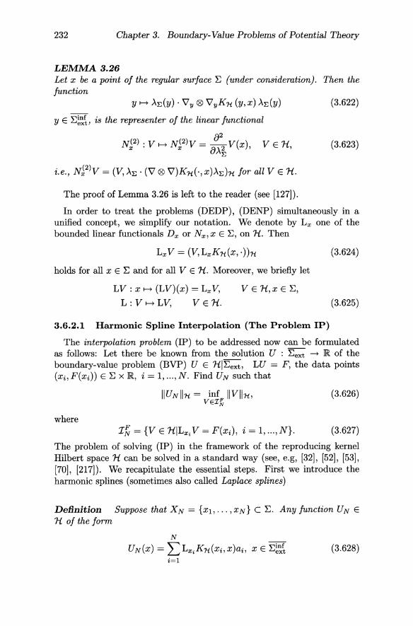
232 Chapter 3. Boundary-Value Problems of Potential Theory
LEMMA 3.26 Let x be a point of the regular surface ~ (under consideration). Then the function
Y f-+ AI;(Y)' '\ly ® '\lyKrt (y,x) AI;(Y)
Y E ~~~t is the representer of the linear functional
N(2) . V f-+ N(2)V = ~ Vex) V E 1i, x' x 8A~ ,
The proof of Lemma 3.26 is left to the reader (see [127)).
(3.622)
(3.623)
In order to treat the problems (DEDP), (DENP) simultaneously in a unified concept, we simplify our notation. We denote by Lx one of the bounded linear functionals Dx or N x , x E ~, on 1i. Then
(3.624)
holds for all x E ~ and for all V E 1i. Moreover, we briefly let
LV: x f-+ (LV)(x) = Lx V, V E 1i,x E~,
L:Vf-+LV, V E 1i. (3.625)
3.6.2.1 Harmonic Spline Interpolation (The Problem IP)
The interpolation problem (IP) to be addressed now can be formulated as follows: Let there be known from the solution U : ~ext ---> ~ of the boundary-value problem (BVP) U E 1i1~ext' LU = F, the data points (Xi, F(Xi)) E ~ X~, i = 1, ... , N. Find UN such that
(3.626)
where It; = {V E 1iILxi V = F(Xi), i = 1, ... , N}. (3.627)
The problem of solving (IP) in the framework of the reproducing kernel Hilbert space 1i can be solved in a standard way (see, e.g, [32], [52], [53], [70], [217)). We recapitulate the essential steps. First we introduce the harmonic splines (sometimes also called Laplace splines)
Definition Suppose that X N = {Xl, ... , XN} c ~. Any function UN E 1i of the form
N
UN(X) = LLxiKrt(xi,x)ai, x E ~~~~ i=l
(3.628)
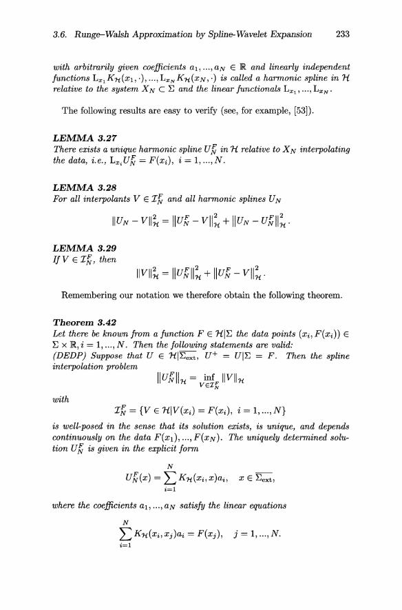
3.6. Runge-Walsh Approximation by Spline-Wavelet Expansion 233
with arbitrarily given coefficients aI, ... , aN E IR and linearly independent functions LXi K 1t (Xl, .), ... , Lx N K 1t (x N , .) is called a harmonic spline in Ji relative to the system X N C E and the linear functionals LXi' ... , LxN •
The following results are easy to verify (see, for example, [53]).
LEMMA 3.27 There exists a unique harmonic spline U~ in Ji relative to X N interpolating the data, i.e., LXi U~ = F(Xi), i = 1, ... , N.
LEMMA 3.28 For all interpolants V E I~ and all harmonic splines UN
LEMMA 3.29 [fV E I~, then
IIVII~ = Ilu~ll~ + IIU~ - vll~· Remembering our notation we therefore obtain the following theorem.
Theorem 3.42 Let there be known from a function F E JiIE the data points (Xi, F(Xi)) E E x 1R, i = 1, ... , N. Then the following statements are valid: (DEDP) Suppose that U E 1t1Eext, U+ = UIE = F. Then the spline interpolation problem
IIU~II'U = inf 11V111t ,. VEX}:;
with
is well-posed in the sense that its solution exists, is unique, and depends continuously on the data F(XI), ... , F(XN). The uniquely determined solution U ~ is given in the explicit form
N
U~(x) = LK1t(xi,x)ai, X E Eext' i=l
where the coefficients aI, ... , aN satisfy the linear equations
N
LK1t(Xi,Xj)ai=F(xj), j=1, ... ,N. i=l
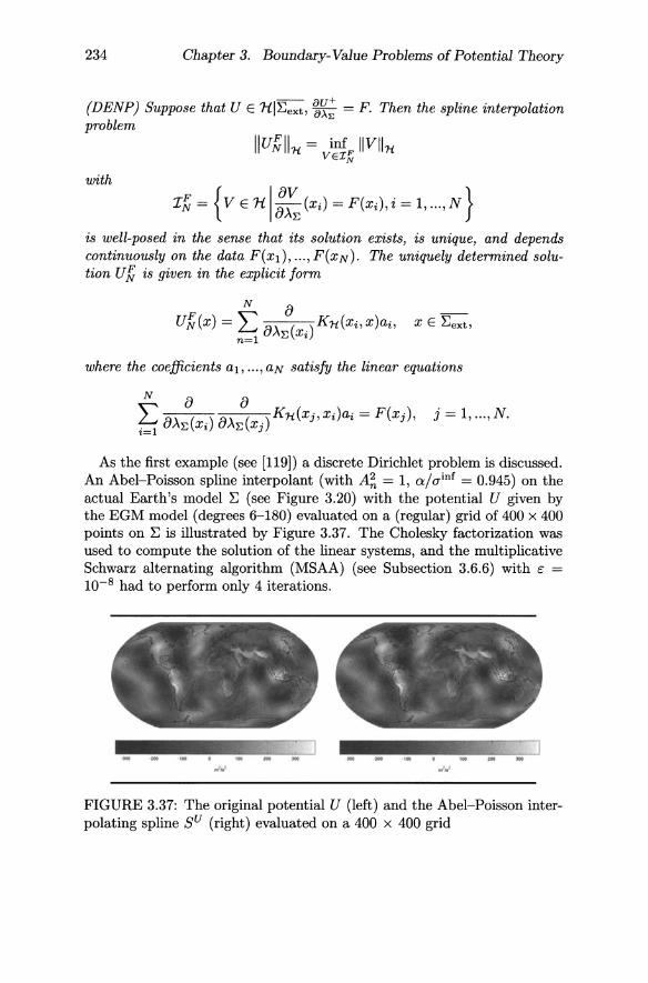
234 Chapter 3. Boundary-Value Problems of Potential Theory
(DENP) Suppose that U E HIEext, ~~; = F. Then the spline interpolation problem
with
Ifr = { V E H I :: (Xi) = F(Xi), i = 1, ... , N }
is well-posed in the sense that its solution exists, is unique, and depends continuously on the data F(xd, ... ,F(XN)' The uniquely determined solution U fr is given in the explicit form
where the coefficients aI, ... , aN satisfy the linear equations
As the first example (see [119]) a discrete Dirichlet problem is discussed. An Abel-Poisson spline interpolant (with A;; = 1, a/ainf = 0.945) on the actual Earth's model E (see Figure 3.20) with the potential U given by the EGM model (degrees 6-180) evaluated on a (regular) grid of 400 x 400 points on E is illustrated by Figure 3.37. The Cholesky factorization was used to compute the solution of the linear systems, and the multiplicative Schwarz alternating algorithm (MSAA) (see Subsection 3.6.6) with c = 10-8 had to perform only 4 iterations.
FIGURE 3.37: The original potential U (left) and the Abel-Poisson interpolating spline SU (right) evaluated on a 400 x 400 grid
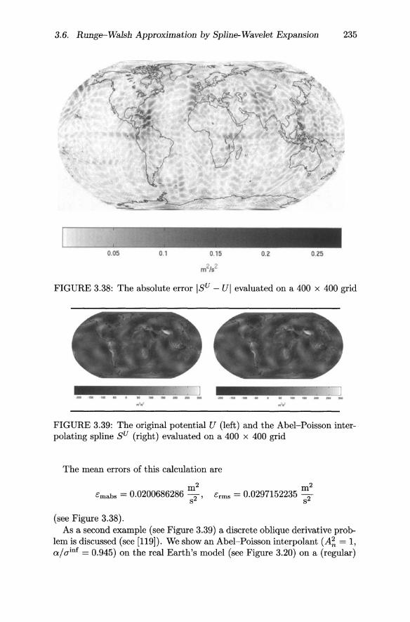
3.6. Runge-Walsh Approximation by Spline-Wavelet Expansion 235
0.05
FIGURE 3.38: The absolute error ISu - UI evaluated on a 400 x 400 grid
FIGURE 3.39: The original potential U (left) and the Abel-Poisson interpolating spline SU (right) evaluated on a 400 x 400 grid
The mean errors of this calculation are
m2 Cmabs = 0.0200686286 2 ,
s
(see Figure 3.38).
m2 Crms = 0.0297152235 2 s
As a second example (see Figure 3.39) a discrete oblique derivative problem is discussed (see [119]). We show an Abel-Poisson interpolant (A; = 1, a/ainf = 0.945) on the real Earth's model (see Figure 3.20) on a (regular)

236 Chapter 3. Boundary-Value Problems of Potential Theory
0.5
FIGURE 3.40: The absolute error ISu - UI evaluated on a 400 x 400 grid
400 x 400 point grid. The directions of the oblique derivatives result from AE(X) = (V'U)(x)/I(V'U)(x)l, x E E, with the potential U given by the EGM96 model (degrees 8-150). Again Cholesky factorization was used, and the MSAA (see Subsection 3.6.6) with € = 10-8 had to perform 45 iterations (for more detail see [119]).
The mean errors of this calculation are
m2 €mabs = 0.2859133302 2"""'
s
(see Figure 3.40).
m2 €rms = 0.4289448755 2"""
s
3.6.2.2 Harmonic Spline Interpolation (The Problem IPm )
H as defined by (3.612) is a semi-Hilbert space by taking the inner prod-uct (., ·hl-L corresponding to the seminorm
O,o",m
( )1~
00 2n+l 2 a 2n -. - inf 2
11V1I'Hif. ... ,m = nf+l f; A;;- C·inf) (VIE~~,H~n-l,j)'H (3.629)
The kernel Ho, ... ,m of this norm II·II'H-L is a linear space of dimension O,o .. ,m
M=(m+l)2.
3.6. Runge-Walsh Approximation by Spline-Wavelet Expansion 237
The interpolation problem (IP m) to be addressed now can be formulated as follows (see [57]): Let there be known from the solution U : ~ext -+ lR of the boundary-value problem (BVP) the data points (Xi, F(Xi)) E ~xlR, i = 1, ... , N, corresponding to an admissible system X N = {Xl, ... , XN} relative to 'lto, ... ,m (Le., a system X N C ~, N ~ M, such that there exists a unique P E 'lto, ... ,m satisfying the interpolating conditions Lx;P = ai, i = 1, ... , M for any prescribed (real) scalars al, ... , aM). Find U~ E 'It such that
IIU~II'H.L = inf IIVII'H.L . 0, ... ,,,, VEIJ:; 0, ... ,,,,
If X N C ~ is an admissible system relative to 'lto, ... ,m, then there is in 'lto, ... ,m a unique basis Bb ... , BM of the form
satisfying (3.631)
For every V E 'It the unique 'lto, ... ,m-interpolant pV of Von the admissible system XM under consideration is given by the "Lagrange formula"
M
pV = ~)Lxi V)Bi' (3.632) i=l
the mapping p : 'It -+ 'lto,: .. ,m is a linear, continuous projector of 'It onto 'lto, ... ,m, and p determines the following direct sum decomposition:
0.L 'It = 'lto, ... ,m EB 'lto, ... ,m (3.633)
with
'It.L -'It.L A ~ . ~inf o 0 (( (inf)n)_) O, ... ,m - O, ... ,m n a 'ext (3.634)
= {V E 'It I Lx; V = 0, i = 1, ... , M}
ii~ ... ,m' as defined by (3.634) equipped with the inner product (" ')'Ht, ... ,,,, '
is a Hilbert space. It is easily verified that iiL.,m has the reproducing
kernel K ° 1. • ~inf X ~inf -+ lR given by 'Ho, ... ,,,,· ext ext
M
KHt, ... ,'" (X, y) = K'Ht, ... ,,,, (X, y) - ~)Lx;K'Ht, ... ,,,, (Xi, X))Bi(Y) i=l

238 Chapter 3. Boundary-Value Problems of Potential Theory
M
- L Bi(x)(LxiK'Hif. ... ,m (y, Xi)) (3.635) i=l
M M
+ L L Bi(X)(LxiLxjK'Hif. .. ,m (Xj, xi))Bj(y), i=l j=l
where
K'Hif. .. ,m (x, y) = f 2:7f:} A;;: 2 (lx~~YI) n+l Pn (I~I . I~I)' (3.636) n=m+l
for x, y E ~~~. Indeed, for eag:h x E ~~~t it is not difficult to show that Kfi.l. (x,·) is a member of 1t~ ... ,m' and the property
O, ... ,Tn
V(x) = (Kfit, ... ,m (x, .), V)'H.l. O, ... ,rn
(3.637)
-- 0 0
holds for every x E ~~~t and V E 1t~ ... ,m' Moreover, in view of the
boundedness of Lx on ii~ ... ,m for x E ~, Y f--+ LxKfit, .. ,m (x, y), y E ~~~t is the representer of Lx.
The problem of finding the smoothest norm interpolant can be solved now by well-known arguments.
Theorem 3.43 Assume that there are known from F E 1t1~ the data points (Xi, F(Xi)) E ~ x ~, i = 1, ... , N. Then the following statements are valid: (DEDP) Suppose that U E 1t1~ext' U+ = UI~ = F. Then the spline interpolation problem
IIU~II'H.l. = inf 11V11'H.l. O, ... ,m VEI~ O, ... ,m
with I~ = {V E 1t1V(Xi) = F(Xi)' i = 1, ... , N}
is well-posed in the sense that its solution exists, is unique, and depends continuously on the data F(Xl), ... , F(XN)' The uniquely determined solution U ~ is given in the form
M N
U~(x)=LF(Xi)Bi(X)+ L Kfiif. .. ,m(xn,x)an, E "inf X LJext,
i=l n=M+l
where the coefficients aM+l, ... , aN satisfy the linear equation
N M
L KfiL,m (xi,Xj)ai = F(xj) - L F(xn)Bn(xj), i=M+l n=l
j = M + 1, ... ,N.

3.6. Runge-Walsh Approximation by Spline-Wavelet Expansion 239
(DENP) Suppose that U E 1i1~ext' ~~; = F such that (3.214) is valid. Then the spline interpolation problem
with
I~ = { V E 1i I :: (Xi) = F(Xi)' i = 1, ... , N }
is well-posed in the sense that its solution exists, is unique, and depends continuously on the data F(XI)' ... , F(XN)' The uniquely determined solution U ~ is given in the form
E "inf X L.iext,
where the coefficients aM+1, ... , aN satisfy the linear equations
j =M +l, ... ,N.
3.6.3 Stability Theorems
Let XN = {Xl, ... , XN} be a subset of ~ with Xi =f:. Xj for i =f:. j. We define the XN-width 8 N by setting
8N=max(min IX-YI). xE~ yEXN
(3.638)
Our purpose (see [57]) is to develop a convergence theorem for the problem (IP m) with increasing N. An analogous result for the problem (IP) is obvious.
Theorem 3.44 Let X N = {Xl"",XN} be an admissible system relative to 1io, ... ,m. Then the following statements are valid: (DEDP) Suppose that U E 1i1~ext' U+ = UI~ = F. Let U~ E 1i be the uniquely determined solution of the problem
where
240 Chapter 3. Boundary-Value Problems of Potential Theory
Then there exists a positive constant D (dependent on 2;) such that
sup IU(x) - U~(x)1 ~ sup IU(x) - U~(x)1 ~ DeNIIUII1i.L . xEEext xEE D, ... ,'m
(DENP) Suppose that U E 'H12;ext, ~~; = F such that (3.214) is valid. Let U~ E'H be the uniquely determined solution of the problem
where
I~ = { V E 'HI :: (Xi) = F(Xi), i = 1, ... ,N } .
Then there exist positive constants C, D (dependent on 2;) such that
PROOF For given x E 2;, there exists a point Xi E X N with Ix - xii ~ eN. In view of Lx,U = LXi UN (with U~ = UN) we find
(3.639)
Since the linear functionals Lx, Lx, on 1t are bounded we get
LxU N - Lx,U N = (LxK1iii"; .. ,,,,, (x,·) - Lx,K1iii"; ... ,,,, (Xi, .), UN )1i.L 0, .. ,Tn
LxU - Lx,U = (LxK1i~ ... ,,,, (x,·) - Lx,K1i~ ... ,,,,, (Xi, .), U)1i.L . O, ... ,Tn
By application of the Cauchy-Schwarz inequality we obtain
(3.640)
where we used the abbreviation
1I1i~ ... ,,,,, (x, Xi) = IILxK1i~ ... ,Jx, .) - Lx, K1i~ ... ,,,,, (Xi, .) II:.L . (3.641) 0, .. ,Tn
UN is the smoothest 'H~ ... ,m-interpolant. Hence, by the triangle inequality, it follows that
1
ILxU N - LxUI ~ 2 (1I1i~ ... ,,,,, (x, Xi)) 2 IIUII1iij-, ... ,,,,. (3.642)
3.6. Runge-Walsh Approximation by Spline-Wavelet Expansion 241
It is not difficult to deduce (see [57]) that
where
Based on estimates for Legendre polynomials (see [57]) we are able to show that there exists a positive constant E (dependent on ~) and a positive polynomial p : No -+~, n f---> p( n) such that
Ibn(x, x) - 2bn(x, Xi) + bn(Xi, xi)l:S E Co-::)2 ) n p(n) Ix - xil2 ,
Ibn(x,y) - bn(Xi,y)l:S E Co-::)2) n p(n) Ix - xii, (3.643)
Ibn (X, y)l:S E ((0-::)2) n p(n)
for all x, y E ~. Therefore, there exists a constant D (dependent on~) such that
(3.644)
This proves Theorem 3.44. I
Theorem 3.44 enables us to approximate the solution U of the preceding boundary-value problem (uniformly on ~ext in a constructive way) using

242 Chapter 3. Boundary-Value Problems of Potential Theory
interpolation by harmonic splines in 'H. provided that the Xwwidths eN tend to O.
Theorem 3.45 Let (XN ) be a sequence of admissible systems relative to 'H.o, ... ,m on ~ such that eN ----> 0 as N ----> 00. Then the following statements are valid: (DEDP) Suppose that U E 'H.1~ext' U+ = UI~ = F. Then, for any prescribed number c: > 0, there exist an integer N = N(c:) and a harmonic spline
M N
UN(x) = L F(xn)Bn(x) + L Kilt, .. ,,,, (x, xn)an , x E ~ext' n=l n=M+l
uniquely determined by
N M
L Kilt, .. ,rn (xn, xj)an F(xj) - L F(xn)Bn(xj), n=M+l n=l
j = M + 1, ... , N, such that
and sup IU(x) - UN(x)1 ~ c:.
xE~ext
(DENP) Suppose that U E 'H.1~ext' ~~; = F such that (3.214) is valid. Then, for any prescribed number c: > 0, there exist an integer N = N(c:) and a harmonic spline
x E ~ext'
uniquely determined by
N f) f) M
L f)AE(X) f)AE(X .) Kilt, .. ,rn (Xj, xn)an = F(xj) - L F(xn)Bn(xj), n=M+l n J n=l
j = 1, ... , N, such that
j = 1, ... ,N,
and sup IU(x) - UN(x)1 ~ c:.
xE~ext
3.6. Runge-Walsh Approximation by Spline-Wavelet Expansion 243
Theorem 3.45 will be exploited to discuss a boundary-value problem of potential theory in its classical formulation U E Pot(O)(~ext)' U+ = F
(resp. U E pot(I'IL)(~ext)' ~~; = F). We already know that the set of all linear combinations of functions LH_n-l,j is dense in C(~) in a uniform sense (for the definition of L see (3.624)). Hence, the set of all functions LV, V E H, is a dense subset of C(~) and C(O,IL) , too. Moreover, an extended version of Helly's theorem due to [222] shows us that, for any G E C(~) and any system XN = {Xl, ... , XN} on~, there exists an element LV, V E H, in an c-neighborhood of G with Lx; V = G(Xi), i = 1, ... , N.
Combining these results we obtain the following theorem.
Theorem 3.46 Let XT = {Xl, ... , XT} c ~ be an admissible system relative to Ho, ... ,m- Suppose that (XN) is a sequence of admissible systems X N relative to Ho, ... ,m
on ~ such that X T C X N for all N and eN ---t 0 as N ---t 00. Then the following statements are valid: (DEDP) For given F E C(~), let U satisfy U E Pot(O)(~exd, U+ = F. Then, for any prescribed c > 0, there exist an integer N = N(c) and a harmonic spline
M N
UN(x) = L F(Xi)Bi(X) + L KH~ .,n> (x, xn)an , X E ~ext' i=l n=M+I
such that
and
sup IU(x) - UN(x)1 :::; C. xEEext
(DENP) For given F E C(O'IL)(~), 0 < J-t :::; 1, let U satisfy U E pot(I'IL)(~exd, ~~; = F such that (3.214) is valid. Then, for any prescribed c > 0, there exist an integer N = N(c) and a harmonic spline
X E ~ext'
such that
j = 1, ... ,T,
and
sup IU(x) - UN(x)1 :::; C.
xEEext
244 Chapter 3. Boundary-Value Problems of Potential Theory
Thus, the justification is given for the use of harmonic splines as a basis system in uniform approximation of classical boundary-value problems of potential theory.
3.6.4 Some Kernel Representations
The procedure of evaluating a harmonic spline interpolant by solving the corresponding system of algebraic equations can be performed simply by standard algorithms, based, for example, on the idea of Cholesky's factorization, and the whole procedure can be described as a recursive algorithm, the data relative to the various interpolation points being exploited in sequence (see [192] and the references therein). The problem remaining is to find suitable reproducing kernel representations (3.610) that are both applicable in boundary-value approximation and (possibly) available as elementary functions (see [57], [214]). Some examples are already known:
(a) A; = 1, n = 0,1, ... (Abel-Poisson kernel)
The reproducing kernel allows the elementary representation
1 IxI21YI2 a 4
K'H(x, y) = 47r (L(x, y~)~ , L(x, y) = Ixl21Yl2 - 2(x· y)a2 + a4 •
(b) A; = (2n + 1)/2, n = 0, 1, .. ("singularity kernel") The reproducing kernel now reads as follows:
K (x ) _ ~ 1 'H ,y - 27r(L(x,y))~·
(c) A; = (2n + l)(n + 1), n = 0,1, ... Now we have
K'H(x,y) = 47r1a 2In (1+ M~~~Y))' M(x,y)=(L(x,y))~+lxllyl-a2. (d) A; = n + 1, n = 0,1, ...
Apart from a multiplicative constant IIVII'H may be understood simply to be equal to the total "energy" stored in the outer space Aext of the sphere around the origin with radius a:
The reproducing kernel admits the representation:
1 (2a2 ( 2(2 ) ) K'H(x, y) = -4 2 1 -In 1 + M( ) . 7ra (L(x,y))2 X,y

3.6. Runge-Walsh Approximation by Spline-Wavelet Expansion 245
The explicit expressions (8j8>.(x))(8j8>.(y))KIt(x,y) can be found in [57]. Furthermore, the thesis [127] gives explicit representations of the expressions (8j8>.(x))2 (8j8>.(y))2 K1t(x, y) which are needed (see Subsection 5.4.1.1) in the context of ill-posed satellite problems.
The "choice of the norm" in spline solutions of boundary-value problems has been investigated thoroughly, e.g., in [57], [58]. Numerical tests on representative examples have shown that interpolation (smoothing) by harmonic splines turns out to be an efficient approximation method of "osculating character" in Dirichlet's as well as Neumann's boundary-value problems of potential theory.
3.6.5 A Tree Algorithm Based on Spline-Wavelets
In what follows the exterior boundary-value problems of potential theory corresponding to Dirichlet's and Neumann's boundary values will be solved exclusively within a multiscale procedure by the use of harmonic interpolating splines (see also [64] and the references therein).
Suppose that a set {al, ... , aN} of N values ai, i = 1, ... , N (with N suitably large), corresponding to the linear (observational) functionals Lx1 , ••• ,LxN is known from a potential V satisfying the assumptions of DEDP resp. DENP (formulated in Subsection 3.6.1): LXi V = ai, i = 1, ... , N. Then there is a member U (i.e., a Runge-Walsh approximation of the potential) of class 7-i such that UI~ext is in an (c:j3)-neighborhood to V (understood in the uniform sense of ~ext) and LxiU = LXi V = ai, i = 1, ... ,N.
Suppose now that 'PI = 'P~ is the generator of a scaling function (as defined in Section 3.5). Consider the family {(<I>?)(2)}, j E Z, of bilinear kernels
00 2n+1 (( D) ( ))2 (<I>D) (2) ( ) = ~ ~ 'Pj n HC< ( )HC< ( )
J X, Y L...; L...; A2 -n-l,k X -n-l,k Y n=O k=l n
(3.645)
00 2n+1 (( D) ( ))2 2 = ~ ~ 'Pj n (~) n H ainf (X)Hainf ()
L...; L...; A2 (TIllf -n-l,k -n-l,k Y n=O k=l n
_ 00 2n+ 1 (('P?) (n))2 (~)n+l ~ (~ . .JL) - ~ 41ra2 A~ Ixllyl n Ixl Iyl '
(x,y) E ~~~~ x ~~~~. There exists an element (<I>~)(2)*1t U such that the restriction ((<I>~)(2) *1t U)I~ext may be considered in (c:j3)-accuracy to UI~ext' and, in addition, LXi((<I>~)(2) *1t U) = LxiU = LXiV = ai, i = 1, ... , N. Note that the representation of (<I>?) (2) (., .) always converges due to the summability condition (3.605) on the sequence (An) and the admissibility condition on 'P~.

246 Chapter 3. Boundary-Value Problems of Potential Theory
From our spline approach we know that an interpolating spline function (oI>D)(2)* u
UL ~J, ... ,t NJ (for suitably chosen integer J and NJ ::::: N) can be found Xl xNJ
such that its restriction to I;ext is in an (c/3)-neighborhood to (<I>~)(2) *'H
UII;ext and
i=l, ... ,NJ .
Note that, in the terminology of Sobolev spaces, (<I>~)(2) is the unique
reproducing kernel of H((An/(<I>~Y\(n)); Aext)II;~'i~. By convention, we let xfJ = Xi, i = 1, ... ,NJ .
In other words, corresponding to the potential V, there exists in caccuracy on I;ext an H-spline consistent with a discrete set of N J original data al,"" aNJ' Consequently, using the Runge-Walsh approximation property and the extended version of Helly's theorem it suffices to approximate a suitable Runge-Walsh potential U E H of the potential V, and it may be assumed that the boundary values come from an interpolating
(oI>D)(2)* u spline U J 'Ii given by
L NJ, ... ,L NJ Xl x NJ
(3.646)
Note that
(3.647)
... ,
is assumed to be a sequence of bounded (linearly independent) linear functionals on H.
As preparation for the development of a tree algorithm (pyramid scheme) some basic facts should be listed (see [64]). First it is clear that the scale spaces
Vj = { G E H I G = (<I>~) (2) *'H U, U E H}
can be rewritten in the form
where I\'Ii _ -1 ( a)n a inf
G (n, k) - G *'H An a inf H-n-l,k'
(3.648)
(3.649)
(3.650)
3.6. Runge-Walsh Approximation by Spline-Wavelet Expansion 247
n = 0,1, ... , k = 1, ... , 2n + 1. Thus the scale space Vj can be identified
with 1i((An('P~(n))-2); Aext)I~~~ that is a reproducing kernel (Sobolev) Hilbert space equipped with the inner product
(3.651)
and the reproducing kernel
(3.652)
00 2n+1 (( D) ( ))4 2 = '"' '"' 'Pj n (~) n H ainf (X)Hainf () ~ ~ A2 amf -n-1,k -n-1,k Y
n=O k=l n
As the symbol of the discrete scaling function satisfies the condition
(3.653)
for all n = 0, 1, ... , it follows that
(( ( D )-2) -) -. f Vj = 1i An 'Pj (n) ; Aext I~~~t (3.654)
1/2 (( (D )-1) -) -. f C Vj = 1i An 'Pj (n) ; Aext I~~~t·
Moreover, the Hilbert space V]/2 as defined by the right hand side of (3.654) is a reproducing kernel Hilbert space with the inner product
(3.655)
and the reproducing kernel
~ 2~1 ('P~(n))2 ( a )2n ainf a inf KV]/2(X, Y) = ~ ~ A2 a inf H- n - 1,k(X)H_n - 1,k(Y)
n=O k=l n (3.656)
The key ideas of our spline-wavelet oriented tree algorithm (pyramid scheme) are based on the following observations:
(1) Corresponding to a potential U E 1i there exists a J-Ievel approximation (<p~)(2) *1t U such that the difference between U and (<p~)(2) *1t U is negligible (for our computational purposes). As a member of class
Vy2, the function (<p~)(2) *1t U may be replaced by a spline inter-( q,D)(2) * u
Polant U J 1i with negligible error. L NJ , ..• ,L N J Xl x NJ

248 Chapter 3. Boundary-Value Problems of Potential Theory
1/2 In other words, we assume U to be a member of class V J so that
( D)(2) ( D)(2) U = <T> J *Vl/2 U ~ <T> J *'H U J
(3.657)
(with suitably chosen J and N J :::; N).
(2) For j = 0, ... , J, we assume that the coefficients w[l, have been determined by solving the linear systems
N j
'" ( D)(2) (N. N.) N· L....,L NjL Nj <T>j xiJ,xZ J wde =bik, l=l Xi Xl '
(3.658)
i, k = 1, ... , N j . The coefficients W[k are computed in an a priori step and stored elsewhere. (Note that the numerical availability of
the coefficients wi'k certainly is the most problematical step within this type of a pyr~mid scheme.)
The initial step. The point of departure for the pyramid scheme is the observation that
U(x) ~ (<T>~)(2) (x,·) *'H U (3.659)
E ~inf X Llext,
where
(3.660) Note that
NJ NJ = "''''L NJ ((<T>~)(2) *'HU)L NJL NJ (<T>~/2) (xfJ,xf'J)wf't L...., L...., X k Xl Xi '
i=l k=1
=Lx~J(<T>~)(2)(,xfJ)*'HU, l=l, ... ,NJ'
In the same way we discretize (\lT~_1)(2)*'HU by using for every U E VJi2
( D)(2)
(\lTD ) (2) * U ~ (\lTD ) (2) * U q, J *'H. U J-l 'H J-l 'H LNJ LNJ
Xl , ... , xNJ (3.661)
3.6. Runge-Walsh Approximation by Spline-Wavelet Expansion 249
The pyramid step. For all F E Vy2 and U E Vy2 we find
F *1i U = (( <I>~) (2) *VY2 F) *1i U
= F *V]/2 (( <I>~) (2) *1i U) (3.662)
With a linearly independent system of bounded linear functionals L Nj' ... ' Xl
LN. on VJ/2 we obtain XN~
( q,D)(2) * u U J 'H. LxNj, ... ,LxNj
1 Nj
(3.663)
h h ffi . N (Nj Nj)T. d t . d b th were t e coe Cient vector a j = ai , ... , aN. IS e ermIne y e J
linear system
N
L L Nj L Nj (<I>~) (2) (x~j ,x~j) a~j = L Nj (( <I>~) (2) *1i U) , i=l X k xi X k
k = 1, ... , N j , i.e.,
(3.664)
(3.665)
Replacing (<I>~)(2) *1i U in (3.662) by the VJ/2-spline interpolant (3.663) leads us to the discretized formula
N j
F*1i U ~ L (LxNjF) a~j i=l •
(3.666)
for all F E VJ/2. The last formula (3.666), in particular, holds true for
the functions (<I>~)(2)(X, .), (\[f~)(2)(X,.) E Vy2 with x E E~'i~ fixed but arbitrary. The recurrence relation of the desired pyramid step now follows
1/2 -.-from the observation that (<I>~)(2)(x,.) E Vj+1 for all x E E~';!t such that
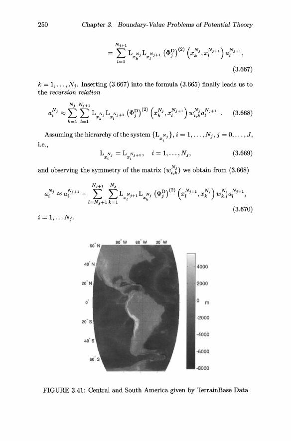
250 Chapter 3. Boundary-Value Problems of Potential Theory
(3.667)
k = 1, ... , N j . Inserting (3.667) into the formula (3.665) finally leads us to the recursion relation
(3.668)
Assuming the hierarchy ofthe system {L Nj}, i = 1, ... , N j , j = 0, ... , J, Xi
i.e., L N =L N"+l, i=l, ... ,NJ"'
Xi J Xi J (3.669)
and observing the symmetry of the matrix (w~k) we obtain from (3.668)
i = 1, ... N j .
4000
FIGURE 3.41: Central and South America given by TerrainBase Data
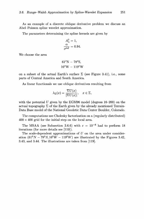
3.6. Runge--Walsh Approximation by Spline-Wavelet Expansion 251
As an example of a discrete oblique derivative problem we discuss an Abel~Poisson spline wavelet approximation.
The parameters determining the spline kernels are given by
We choose the area
A~ = 1, a
-.-f = 0.94. a lll
61°N - 78°S,
16°W - 119°W
on a subset of the actual Earth's surface ~ (see Figure 3.41), i.e., some parts of Central America and South America.
As linear functionals we use oblique derivatives resulting from
'VU(x) A~(X) = l'VU(x) I ' x E ~,
with the potential U given by the EGM96 model (degrees 16~200) on the actual topography ~ of the Earth given by the already mentioned TerrainData Base model of the National Geodetic Data Center Boulder, Colorado.
The computations use Cholesky factorization on a (regularly distributed) 400 x 400 grid for the initial step on the local area.
The MSAA (see Subsection 3.6.6) with c = 1O~8 had to perform 18 iterations (for more details see [119]).
The scale-dependent approximations of U on the area under consideration (61 0 N - 780 S, 160 W - 1190 W) are illustrated by the Figures 3.42, 3.43, and 3.44. The illustrations are taken from [119].
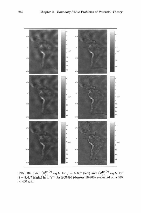
252 Chapter 3. Boundary-Value Problems of Potential Theory
FIGURE 3.42: (<I>~) (2) *1t U for j = 5,6,7 (left) and (w~) (2) *1t U for j = 5,6,7 (right) in m2s-2 for EGM96 (degrees 16-200) evaluated on a 400 x 400 grid
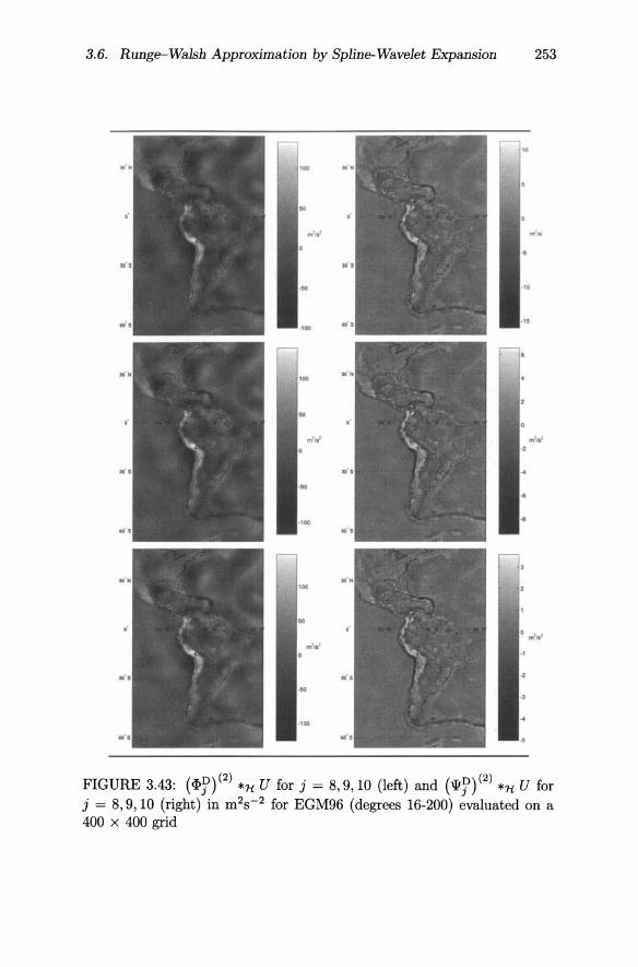
3.6. Runge-Walsh Approximation by Spline-Wavelet Expansion 253
FIGURE 3.43: (<[>~)(2) *1t U for j = 8,9,10 (left) and (W~)(2) *1t U for j = 8,9,10 (right) in m2s-2 for EGM96 (degrees 16-200) evaluated on a 400 x 400 grid
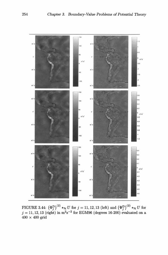
254 Chapter 3. Boundary-Value Problems of Potential Theory
FIGURE 3.44: (<I>~)(2) *11. U for j = 11,12,13 (left) and (W~)(2) *11. U for j = 11,12,13 (right) in m2s-2 for EGM96 (degrees 16-200) evaluated on a 400 x 400 grid

3.6. Runge-Walsh Approximation by Spline-Wavelet Expansion 255
3.6.6 Multiplicative Schwarz Alternating Algorithm (MSAA): A Domain Decomposition Method
In what follows we are interested in discussing how the linear systems occurring in our spline and/or wavelet approach can be solved numerically. We start from a linear system with a positive definite symmetric matrix (see [76], [119] for more details):
Ax=b,
where
A E !R.NXN, AT = A, Ay· y > 0, y E !R.N\{O}, x, bE !R.N. (3.671)
Such a linear equation system can be solved with iterative solvers or direct solvers, but if N is large (for example, N ~ 10,000), the runtime of an iterative solver without a suitable preconditioner or of a direct solver increases tremendously. This is the reason why we need a more sophisticated method to solve the linear system (3.671) for problems with a large number of given data.
One such method is a multiplicative variant of the Schwarz alternating algorithm, a domain decomposition method, which allows it to split the matrix A in (3.671) into several smaller submatrices, which generally may (and will in numerical implementations) overlap. This multiplicative variant of the Schwarz alternating algorithm is an iterative method which solves in each iteration step linear systems with the matrices obtained from the splitting successively. This reduces both runtime and memory requirements drastically.
The Schwarz alternating algorithm dates back to H. A. Schwarz' work [203], published in 1890, and has been investigated by many authors since then. A revived interest in variants of Schwarz alternating method arose since 1985, due to the availability of fast modern and parallel computers. Roughly speaking, there are mainly two types of Schwarz alternating algorithms: multiplicative variants (like the one used here) and additive variants, which can be implemented on parallel computers and are usually faster. For more information about the Schwarz alternating algorithm, the reader is referred to, for example, [148], [149], [150], [221] and the references therein. In the last few years, a great interest has also been taken in the relation between the Schwarz alternating algorithm, multisplittings, multigrid methods, preconditioned conjugate gradient methods, and other iterative schemes (see, for example, [18], [31], [76], [109], [115], [116], [127]).
The solution of the linear system (3.671) with a multiplicative variant of the Schwarz alternating algorithm, which will be called the multiplicative Schwarz alternating algorithm (MSAA), is based on two facts: (i) every positive definite symmetric matrix is a Gram matrix, and (ii) the

256 Chapter 3. Boundary-Value Problems of Potential Theory
convergence proof of the MSAA is based on its formulation in terms of orthogonal projectors.
According to our assumptions, the matrix A = (Ai,j kj=l, ... ,N in the linear system (3.671) is positive definite and symmetric. Due to the theorem about the Cholesky factorization (see, for example, [121]), there exists a uniquely determined invertible lower triangular matrix L with positive diagonal entries, such that
(3.672)
Denote the row vectors of L by Vb' .. , VN. Then (3.672) implies (see [76], [127]) that
i,j=l, ... ,N.
Thus, A is the Gram matrix of the basis {Vl,"" V N} of JR.N, and the solution x = (Xl, ... ,XN)T of the linear system (3.671) is the solution of the following orthogonal projection problem: Find X = (Xl, ... , X N ) T E JR.N such that f E JR.N with f . Vi = bi , i = 1, ... , N, has the representation
N
f = LXiVi.
i=l
(3.673)
Indeed, the solution of this problem demands the solution of the linear system
N
LXi (Vi' Vj) = f . Vj = bj , j= 1, ... ,N, (3.674) i=l
which is just the linear system (3.671). The orthogonal projection operator corresponding to (3.673) is, of course, the identity operator: We seek a representation of f = Id]RN f with respect to the basis {Vl, ... , VN}. Now we split the basis {Vl, ... , V N} into several smaller, possibly overlapping subsets '2~r = {vI, ... , viVJ C {Vl"'" VN}, r = 1, ... , M, such that
M
U -;:::Nr - { } ~r - Vl"",VN .
r=l
This union will, in general, not be disjoint, and we speak of overlapping subsets if there are at least two subsets '2~r, '2~k with '2~r n '2~k i=- 0 and k i=- r.
Denote the orthogonal projector from JR.N onto span ('2~r) by
Pr : JR.N -+ span{ v~, ... , viVJ ' 9 I-t Prg, (3.675)
i.e., Pr = Pr 0 Pr and Prv . W = V • Prw for all v, W E JR.N. In order to compute Pr g, we assume again that 9 . Vi, i = 1, ... , N, is known. We want
3.6. Runge-Walsh Approximation by Spline-Wavelet Expansion 257
to calculate the coefficient vector Y = (Y1,' .. ,YNr ) of the representation
N r
Prg = LYi V[ . i=l
Taking the inner product with vr, ... ,vj\rr successively leads to the linear system
j = 1, ... ,Nr . (3.676)
Clearly, the matrix Ar = (vi, vjkj=l, ... ,Nr is a submatrix of the matrix A of the linear system (3.671).
We will now formulate the MSAA for the solution of the trivial orthogonal projection problem Id]RN f = f in terms of the orthogonal projectors Pr' For this algorithm we prove the convergence and give information about the convergence rate (see [76], [127]). After that, we will transform this algorithm into a matrix formulation which solves (3.674) by solving alternatingly the problems of the type (3.676).
Algorithm 3.1 (Multiplicative Schwarz Alternating Algorithm) Set fa = f E ffi.N and S6 = ° for n = 0,1,2, ... do
for r = 1, ... ,M do
calculate S~M+r = S~M+(r-1) + Pr(fnM+(r-l))
update fnM+r = fnM+(r-1) - Pr (fnM+(r-1»)
t'l I (f(n+I)M . VI, .. · .J(n+I)M . VN )TI < unz 1(f'VI, ... ,f'VN)TI _c.
Next, we show that the sequence of iterates {S~M }nENo converges to f for n --+ 00. The following lemma is very helpful for the understanding of Algorithm 3.1.
LEMMA 3.30 Let the notation and the assumptions be the same as in Algorithm 3.1, and denote the orthogonal projection onto the space (span{ vr, ... ,vj\rJ).i, where r E {1, ... ,M}, by Qr: ffi.N --+ span{vr, ... ,vj\rJ).i, i.e., Qr = JdPr' Then the following identities are valid for all n E No, r E {1, ... , M}:
. f _ r n-1 M (z) snM+r - I: Pj (fnM+(j-1») + I: I: Pj(fIM+(j-1») '
j=l 1=0 j=l
(ii) fnM+r = f - S~M+r'
( ... ) f - f ~ (f f ) ZZZ snM+r - snM+(r-1) + r - snM+(r-1) ,
258 Chapter 3. Boundary-Value Problems of Potential Theory
(iv) fnM+r = (Qr··· Q1) (QM··· Qdn f,
(v) S~M+r = f - (Qr··· Q1) (QM··· Qdn f·
PROOF The identities (i), (ii), and (iv) follow a straightforward proof by induction, whereas (iii) and (v) are simple consequences of (i), (ii), and (iv). The proof can, for example, be found in [127]. I
Looking at the identities (i) through (iii), we see that Algorithm 3.1 has the standard structure of an iterative algorithm: We start with fo = f, s6 = 0 and compute s{ = P1 (J), where P1 is an approximation of Id]RN. Then we calculate the residual h = f - P1 (J). After that we compute P2 (Jd = P2 (J - s{), where this time P2 is used as an approximation of Id]RN. Then we calculate the new iterate s~ = s{ + P2 (h) and the new residual h = f - s~ = h - P2 (h). This process is repeated using successively P3, ... ,PM as approximations of Id]RN. Then the first iterative step is completed, and we start again with P1 and proceed in the same fashion as before:
S~M+r = S~M+(r-1) + Pr(J - S~M+(r-1)) .
In order to get the new iterate S~M+r' we solve the problem approximately
for the residual fnM+(r-l) = f - S~M+(r-1) and add this solution to the
old iterate S~M+(r-1)" But in contrast to standard iterative algorithms the approximate solution is alternatingly computed with P1, ... , PM.
The identities (iv) and (v) in Lemma 3.30 are important for the convergence proof of Algorithm 3.1. Identity (v) shows that the approximation error of S~M is given by
(3.677)
The convergence ofthe residual {fnM }nENo to zero for n ---+ 00 follows either from the following theorem about the product of orthogonal projection operators or can be proved in an elementary way.
Theorem 3.47 Let H be a Hilbert space with inner product (., ·hi, let Ul, ... ,UM be closed subspaces of H, and let Qi : H ---+ Ui, i E {I, ... , M}, be the orthogonal projector onto Ui. Denote by P : H ---+ n:!l Ui the orthogonal projector
onto n:!l Ui , and define Q : H ---+ H by Q = QM··· Q1. Then {Qn}nENo converges pointwise to P, i.e.,
lim IIQn F - PFII1{. = 0 for all FE H. n-+oo
3.6. Runge-Walsh Approximation by Spline-Wavelet Expansion 259
PROOF This theorem is a special case of the results in [120j. I
COROLLARY 3.8 Let the notation and the assumptions be the same as in Algorithm 3.1 and Lemma 3.30. Then the sequence {S~M }nENo of iterates of a vector f E ]RN
converges to f.
PROOF According to Lemma 3.30
lim If - s~MI = lim I(QM ... Qdn fl = IPfl, n~oo n----+-oo
where P is the orthogonal projector P : ]RN ----> ]RN onto n~1 (im (Qr)). But
M M n im(Qr) = n (span {vL···, v~J)~ r=1 r=1
~ (t, 'pon { v;' , v;'.l r (3.678)
= (]RN)~ = {O}.
Hence P = 0 and limn->co If - s~MI = O. The equality of (3.678) follows from the following statement: Let 1{ be a Hilbert space with inner product (., ·h-l and let VI' ... ' VM be M closed subspaces of 1{. Then
(3.679)
where
t, Vi = span {Q Vi} . (3.680)
The inclusion C is obvious, and J follows because F E n~1 vi- is also
orthogonal to every element in span{U~1 Vi}. I
As mentioned before, there is also a second proof of the convergence of Algorithm 3.1, which uses only elementary results from functional analysis and yields convergence in the operator norm and an estimate of the convergence rate (see [76], [127]).
Theorem 3.48 Let the notation and the assumptions be the same as in Algorithm 3.1 and Lemma 3.30. Then the sequence {S~M }nENo of iterates of a vector f E ]RN
260 Chapter 3. Boundary-Value Problems of Potential Theory
converges to f, and the error estimate
with some constant C < 1, independent of f, is valid.
PROOF According to Lemma 3.30, for all n E N
(3.681)
For simplicity of notation, we denote Q = Q M ... Ql. The proof is complete if we can show that IIQII < 1. As all Qr, r E {1, ... , M}, are orthogonal projectors, IIQrl1 ~ 1, and, consequently,
M
IIQII = IIQM ... Qlll ~ II IIQrl1 ~ 1. (3.682) r=1
We show now, that the assumption IIQII = 1 leads to a contradiction. If
1 = IIQII = sup IQgl (3.683) 9EJRn,191=1
there exists a sequence {9n}nEl'l C ]RN with 19n1 = 1 for all n E Nand
lim IQgnl = 1. (3.684) n---+oo
The space ]RN is finite dimensional and has, therefore, a compact unit sphere. Hence {gn}nEl'l has a convergent subsequence {gn"jmEl'l, whose limit 9 E ]RN is a vector with Igl = 1 and
IQgl = lim I Qgn", I = 1. m---+oo
Thus
IQgl = Igl· (3.685)
Now, we show that (3.685) implies that Qrg = 9 for all r E {1, ... , M}: First, observe that the orthogonal projector Qr satisfies for all W E ]RN
IwI2 = IQrw + (IdJRN - Qr )w12 (3.686)
= IQrwl2 + I(IdJRN - Qr)wl 2 ,
because (Qrw, (IdJRN - Qr)w) = O. Equation (3.686) shows that
Iwl = IQrwl is equivalent to I(IdJRN - Qr)wl = O.
3.6. Runge-Walsh Approximation by Spline-Wavelet Expansion 261
This means that
QrW = W is equivalent to IQrwl = Iwi , Qrw of- w is equivalent to IQrwl < Iwl .
Consider now g E ]RN, which satisfies (3.685). Let j E {I, ... , M} be the smallest index for which Qrg of- g. Then, IQjgl < Igl, and thus,
Igl = IQgl = IQM ... Qjgl ~ IIQM . .. Qj+llllQjgl < Igl,
which is a contradiction. Hence, there can be no such j and
Qrg = g for all r E {I, ... , M} . (3.687)
Equation (3.687) implies that g E im( Qr) for all r E {I, ... ,M}:
M M
gE n im(Qr)= n (span{vr, ... ,VNJ)~ r=l r=l
According to (3.680), this is equivalent to
9 E (~,pan{v;, . .. ,VN-.J)" ~ (,pan{VJ,"',VNJ)" ~ (RN)" ~ {OJ
Thus, g = ° which is a contradiction to Igl = 1. Consequently, the assumption IIQII = 1, is wrong. I
Now, we come back to Algorithm 3.1 and transform it into a matrix formulation via (3.674) and (3.676) (see [127]). For this purpose, we need the restriction operators Rr : ]RN -+ ]RNr, W f-t Rr(w) = ((Rr(w)h, ... , (Rr(W))NJT, and the embedding operators Ir : ]RNr -+ ]RN, Z f-t Ir(z) = ((Ir(z)h, ... , (Ir(Z))N)T, corresponding to the subspaces ]RNr of the subproblems (3.676). They are defined by
(Rr(w))i = Wj for the index j E {I, ... , N} with v[ = Vj ,
(Ir(z)). = {Zj if ther~ exists j E {I, ... , Nr } with vj = Vi t ° otherwIse.
Algorithm 3.2 (Matrix Formulation of Algorithm 3.1) Define the matrices Ar = (v[· Vjkj=I, ... ,Nr , r = 1, ... M
set fo = (J. VI,· .. , f· VN)T, ao = (0, ... ,O)T E ]RN, where f E]RN
for n = 0,1,2 ... do
262 Chapter 3. Boundary-Value Problems of Potential Theory
for r = 1, ... ,M do solve Ar d = Rr(JnM+(r-l)), d = (d1 , ... , dNJT E ]RNr
update anM+r = anM+(r-l) + Ir(d)
updat' f.M+" ~ I.M +("-'l - ( C~ d; vi . Vk) kO' .... ,N) T
t 'l li(n+l)MI < un Z _ E Ifol -
M
compute S{n+l)M = L) a(n+l)M)i Vi . i=l
It remains to show that Algorithm 3.2 solves our initial problem A x = b, where f E ]RN in Algorithm 3.2 satisfies f . Vj = bj , j = 1, ... , N, and where A = (Vi' Vjkj=l, ... ,N.
Beforehand, we stress that all the computations (except the computation of S{n+l)M) in Algorithm 3.2 can be performed without actually computing
VI, ... , VN E ]RN, i.e., we do not need the Cholesky factorization of A. The matrices Ar are available as submatrices of A, and the update involves a matrix vector multiplication with the matrix (Vk' vi) k=l, ... ,N; , which is also
't=l, ...• Nr
a submatrix of A.
COROLLARY 3.9 Let the notation and the assumptions be the same as in Algorithm 3.2. Then the sequence {anM }nEl\!o C ]RN in Algorithm 3.2 converges to the solution x E]RN of the linear system Ax = b, where A = (Vi' Vjkj=l, ... ,N and b = (f . VI, ... ,J . V N ) T .
PROOF According to Theorem 3.48 and Equations (3.674) and (3.676),
we know that {S~M }nEl\!o
N
S~M = L)anM)i Vi, i=l
converges to f = 2:[:1 Xi Vi, where x is the solution of Ax { VI, ... , V N} is a basis of ]R N this implies that
lim (anM)i = Xi for i = 1, ... , N. n-+oo
This proves the convergence. I
b. As
Finally it should be mentioned that domain decomposition methods as proposed here for solving large linear systems of equations involving the
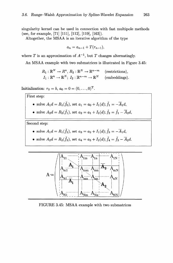
3.6. Runge-Walsh Approximation by Spline-Wavelet Expansion 263
singularity kernel can be used in connection with fast multipole methods (see, for example, [71J [111], [112], [119], [163]).
Altogether, the MSAA is an iterative algorithm of the type
where T is an approximation of A-I, but T changes alternatingly.
An MSAA example with two submatrices is illustrated in Figure 3.45:
R1 :]RN --+ Rn, R2 :]RN --+ ]Rn-m (restrictions),
h :]Rn --+ ]RN; 12 : ]Rn-m --+]RN (embeddings).
Initialization: TO = b, ao = 0 = (0, ... , O)T.
First step:
• solve AId = R 1(Jo), set a1 = ao + h(d); 11 = -AId,
• solve A2d = R2(A), set a2 = a1 + 12(d); 12 = 11 - A 2d,
Second step:
• solve AId = R 1 (J2), set a3 = a2 + h(d);i3 = -AId,
• solve A2d = R 2(J3), set a4 = a3 + 12(d); 14 = 13 - A2d.
I tn ~: .....• 1i.;;·11~· ............. tIN i \ 1rui&·::·:::::lm~·1m~··~2" ~N'
A~= ~l'='" 'An~>:'An~ ..................... ~N ,; l\.., ·······,I. ..... A I i .L
: ! !; :2. ' 'A ············A····A····L·················A , Nl Nm Nn' NN
FIGURE 3.45: MSAA example with two submatrices
264 Chapter 3. Boundary-Value Problems of Potential Theory
3.7 Exercises
3.1 Let x E 1R3 and p > 0 be arbitrary. Prove that the function
1 F : y t--; -I --I' y E {z E 1R3 : Iz - xl > p} ,
x-y
is harmonic.
3.2 Suppose that F, H are of class C(L:). Let v be the outside unit normal field to L:.
(a) Prove: The solution U E Pot(1) (L:int ) with
au av (x) + H(x)U(x) = F(x), x E L:,
is-if it exists-unique, if H ~ O.
(b) Prove: The solution U E Pot(1) (L:ext ) with
au av (x) + H(x)U(x) = F(x), x E L:,
is-if it exists-unique, if H :::; O.
(c) Find examples, where the ~ or :::; condition is not satisfied and the uniqueness is not given, either.
3.3 Let (An)n=O,l, ... , (Bn)n=O,l, ... be real sequences with An =1= 0 =1= Bn for all nand IAnl :::; IBnl for all n. Prove that
3.4 Which of the following systems define a multiresolution analysis in X?
a) Polo, ... ,n([a,b]) := {polynomials on [a,b] with degree:::; n},n E
No; X = (L2[a,b], 11·IIV[a,bj). (a,b E lR,a < b),
b) span{Pdk=o, ... ,n, n E No; X = (L2[-1, 1], II·IIV[-l,lj),
c) span{eik'hEz,k:<:;n, n E No; X = (L2([0, 21f], q, II . IIL2([o,21rj,q) , n
d) Harmo, ... ,n(O) := EB Harmi(O), n E No; X = (L2(O), 11·llv(n)). i=O
Here L2([0, 21f], q stands for the square-integrable complex-valued functions F : [0,21f] ---.. c.
3.7. Exercises 265
3.5 Determine for each system {Vn}nENo in Exercise 3.4 a corresponding system {Wn}nENo of linear spaces, such that Vn+1 = Vn + Wn for all n E No, i.e., Vn+1 = {v + wlv E Vn , w E Wn }. Prove that your systems satisfy the requirements!
3.6 Check which of the systems {Wn }nENo of Exercise 3.5 are orthogonal, i.e., for which system is each pair (Wn' Wm) orthogonal with respect to X?
3.7 Let fJ/ ::; f1, and F, G be of class G(O,IL)(E). Prove the following properties:
(i) 1IFIIL2(E)::; ~IIFllc(E) ::; ~llFllc<o'!")(E)' (ii) IIFGIIC(E)::; 1IFIIc(E) IIGllc(E),
II FGII C(O,!"') (E) ::; 211F11 C(O,!") (E) II Gil C(O,!") (E), (iii) 1IFIIc(o,!"') (E) ::; GIL',IL 1IFIIc(o,!") (E) for some positive constant GIL"w
3.8 Show the limit relation (3.62).
3.9 Verify Lemma 3.28.
3.10 Show the inequality (3.621).
3.11 Let (X, (" .)) be a separable pre-Hilbert space. Assume that (X, (', .) ~) is its completion. Show that there exists a sequence {Xn}n=1,2, ... with the following properties:
(i) Xn E X, n = 1,2, ... ,
(ii) {Xn}n=1,2, ... is complete in X,
(iii) {Xn}n=1,2, ... is not complete in X.
3.12 Let {Xn}x=1,2, ... C Eint be a sequence of distinct points. Prove that both
XI---> ,X E E { 1 } Ix - Xn I n=1,2, ...
and
{XI--->~ 1 'XEE} v(x) Ix - xnl n=1,2, ...
are linearly independent.
3.13 Let E be a regular surface. Show that, for (x, y) E E X E and o < T ::; TO (TO sufficiently small),
( ) I X-TV(X)-Y X-(Y+TV(Y)) I "'r x, Y = Ix _ TV(X) _ YI3 - Ix - (y + Tv(Y))13
266
satisfies
Chapter 3. Boundary-Value Problems of Potential Theory
CTlv(x) - v(y)1 Kr(X, y) :::; Ix _ (y + Tv(y))1 3 '
3.14 Let E be a regular surface. Then
J f) 1 { -41f , x E Eint f)v( ) -Ix _ I dw(y) = 0, x E Eext
E y Y -21f , x E E.