sensors

Technical Note

Non-Contact Measurement of Blade Vibrationin an Axial Compressor

Radoslaw Przysowa 1,* and Peter Russhard 2

1 Instytut Techniczny Wojsk Lotniczych (ITWL), ul. Ksiecia Bolesława 6, 01-494 Warszawa, Poland2 EMTD Ltd., 22 Woods Meadow, Derby DE72 3UX, UK; peter.russhard@emtd-measurement.com* Correspondence: radoslaw.przysowa@itwl.pl

Received: 24 November 2019; Accepted: 19 December 2019; Published: 21 December 2019 �����������������

Abstract: Complex blade responses such as a rotating stall or simultaneous resonances are commonin modern engines and their observation can be a challenge even for state-of-the-art tip-timingsystems and trained operators. This paper analyses forced vibrations of axial compressor blades,measured during the bench tests of the SO-3 turbojet. In relation to earlier studies conducted inPoland with a small number of sensors, a multichannel tip-timing system let us observe simultaneousresponses or higher-order modes. To find possible symptoms of a failure, blade responses in a healthyand unhealthy engine configuration with an inlet blocker were studied. The used analysis methodscovered all-blade spectrum and the circumferential fitting of blade deflections to the harmonicoscillator model. The Pearson coefficient of correlation between the measured and predicted tipdeflection is calculated to evaluate fitting results. It helps to avoid common operator mistakes andmisinterpreting the results. The proposed modal solver can track the vibration frequency and adjustthe engine order on the fly. That way, synchronous and asynchronous vibrations are observed andanalysed together with an extended variant of least squares. This approach saves a lot of work relatedto configuring the conventional tip-timing solver.

Keywords: blade vibration; blade tip-timing; rotating stall; axial compressor; blade health monitoring;least squares; bladed disc dynamics

1. Introduction

Non-contact blade vibration measurement, known as blade tip-timing (BTT) or Non-IntrusiveStress Measurement System (NSMS), is a technique for determining dynamic blade stresses to ensurethe structural integrity of bladed disks in jet engines and stationary turbines [1,2]. It can be used inaxial or radial compressors [3] and unshrouded or shrouded turbines [4]. The method uses severalsensors mounted circumferentially to precisely determine temporary positions of each blade tip inevery rotation [5]. Model-based data processing is necessary to determine the real amplitude andvibration [6,7]. BTT solutions used by industry are still based on algorithms established at the endof the 20th century. Most vibration surveys rely upon traversing each of the resonances. Analysingresponses at a constant speed is more difficult to achieve.

In most applications, undersampled tip deflection signals are generally processed by the twogroups of methods: (1) Fourier spectral analysis, e.g., all-blade spectrum, (2) least squares fitting(LSF). Fourier transform methods compromise time and frequency resolution and involve significantpost-processing to reconstruct the real spectrum. They are now used primarily to identify the presenceof non-integral vibration and to determine nominal frequency and nodal diameter. This data seedsleast squares fitting [8]. LSF is now the main method used in most of BTT systems to extract the realamplitude and phase for successive revolutions. It can be used either circumferentially to fit the blademode or axially to fit the mode shape - each has a different strategy for conversion to stress [9]. The

Sensors 2020, 20, 68; doi:10.3390/s20010068 www.mdpi.com/journal/sensors

Sensors 2020, 20, 68 2 of 18

models for this can be simplistic sine fitting [10] or more complex ones derived from the finite elementmethod (FEM) during the calibration and validation process used with BTT.

Alternative methods introduced in the previous decade such as auto-regressive [11], spectralestimation using nonuniform sampling [12], or full-signal analysis using many points per bladepass [13], were too complex or not efficient enough to leave the labs and be widely used by thecommunity. These alternative methods provide little additional capability to the BTT technology butare often revisited by researchers [14–16] in the hope of finding methods for in-service blade healthmonitoring (BHM), where the blade sets are already well understood.

A significant number of papers, introducing new BTT models and algorithms such as a newtwo-parameter plot method [17], convolutional neural networks [18], aliasing reduction [19,20], sparserepresentation, and compressed sensing [21], were published recently, but they can be applied in reallife to a limited extent. Several newly introduced algorithms work well only with simulated or rigacquired data, usually with a single response of the first mode. Further efforts are needed to makethem more mature to better deal with noise and weak or more complex responses.

Validation against simulation is not accepted for certification of engines [22]. BTT technique wasalready used in component certification tests, where the evidence to calculate a meaningful value ofstress was produced [23]. However, a documented validation of the measurement system and abilityto estimate uncertainty are still missing in many BTT applications.

This paper presents robust and efficient methodology of processing tip-timing data whichproduces vibration results of known and controlled uncertainty. It is demonstrated on two datasetsacquired in a realistic test-cell environment.

First, stack pattern is calculated to check alignment, validate measurement data, and avoidmisinterpreting it, especially when strong low-order excitation force is present. Then, an extendedmethod of least squares is used to analyse coinciding integral and non-integral blade vibrationstogether. The Pearson coefficient of correlation between the measured and predicted tip deflection iscalculated to evaluate fitting results.

Finally, to study interaction between the rotating stall and integral resonance, a new modal solveris used, which can track the modal frequency and adjust the engine order on the fly, producing resultssimilar to strain gauges. Measurement uncertainty is calculated for any point on the tracked orderresponse to assess the overall results.

2. Materials and Methods

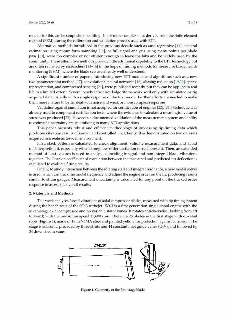
This work analyses forced vibrations of axial compressor blades, measured with tip timing systemduring the bench tests of the SO-3 turbojet. SO-3 is a first generation single-spool engine with theseven-stage axial compressor and no variable stator vanes. It rotates anticlockwise (looking from aftforward) with the maximum speed 15,600 rpm. There are 28 blades in the first stage with dovetailroots (Figure 1), made of 18H2N4MA steel and painted yellow for protection against corrosion. Thestage is subsonic, preceded by three struts and 44 constant inlet guide vanes (IGV), and followed by34 downstream vanes.

Figure 1. Geometry of the first-stage blade.

Sensors 2020, 20, 68 3 of 18

The conducted engine tests were aimed to characterise blade vibrations i.e., identify existingresponses, especially high-order ones. This is often necessary when investigating blade failure inlegacy compressors or turbines, when design data are not available or not reliable.

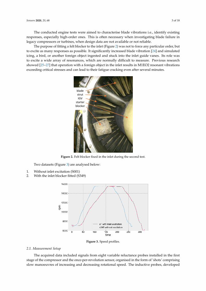
The purpose of fitting a felt blocker to the inlet (Figure 2) was not to force any particular order, butto excite as many responses as possible. It significantly increased blade vibration [24] and simulatedicing, a bird, or another foreign object ingested and stuck into the inlet guide vanes. Its role wasto excite a wide array of resonances, which are normally difficult to measure. Previous researchshowed [25–27] that operation with a foreign object in the inlet results in M1EO2 resonant vibrationsexceeding critical stresses and can lead to their fatigue cracking even after several minutes.

blade strut IGV

starter blocker

Figure 2. Felt blocker fixed in the inlet during the second test.

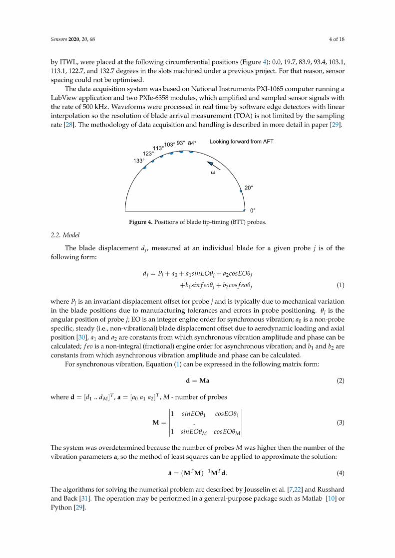
Two datasets (Figure 3) are analysed below:

1. Without inlet excitation (S001)2. With the inlet blocker fitted (S349)

Figure 3. Speed profiles.

2.1. Measurement Setup

The acquired data included signals from eight variable reluctance probes installed in the firststage of the compressor and the once-per-revolution sensor, organised in the form of ’shots’ comprisingslow manoeuvres of increasing and decreasing rotational speed. The inductive probes, developed

Sensors 2020, 20, 68 4 of 18

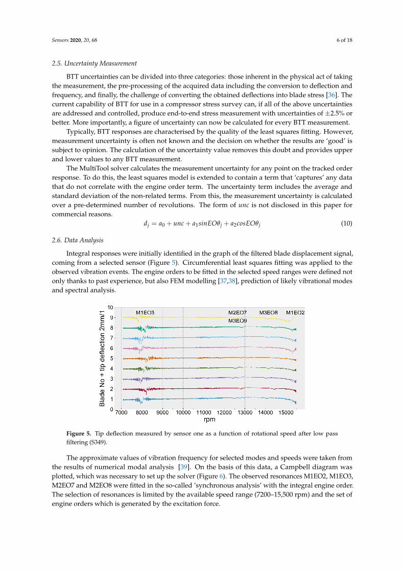
by ITWL, were placed at the following circumferential positions (Figure 4): 0.0, 19.7, 83.9, 93.4, 103.1,113.1, 122.7, and 132.7 degrees in the slots machined under a previous project. For that reason, sensorspacing could not be optimised.

The data acquisition system was based on National Instruments PXI-1065 computer running aLabView application and two PXIe-6358 modules, which amplified and sampled sensor signals withthe rate of 500 kHz. Waveforms were processed in real time by software edge detectors with linearinterpolation so the resolution of blade arrival measurement (TOA) is not limited by the samplingrate [28]. The methodology of data acquisition and handling is described in more detail in paper [29].

0°

20°

84°93°103°113°123°

133°

Looking forward from AFT

Figure 4. Positions of blade tip-timing (BTT) probes.

2.2. Model

The blade displacement dj, measured at an individual blade for a given probe j is of thefollowing form:

dj = Pj + a0 + a1sinEOθj + a2cosEOθj

+b1sin f eoθj + b2cos f eoθj (1)

where Pj is an invariant displacement offset for probe j and is typically due to mechanical variationin the blade positions due to manufacturing tolerances and errors in probe positioning. θj is theangular position of probe j; EO is an integer engine order for synchronous vibration; a0 is a non-probespecific, steady (i.e., non-vibrational) blade displacement offset due to aerodynamic loading and axialposition [30], a1 and a2 are constants from which synchronous vibration amplitude and phase can becalculated; f eo is a non-integral (fractional) engine order for asynchronous vibration; and b1 and b2 areconstants from which asynchronous vibration amplitude and phase can be calculated.

For synchronous vibration, Equation (1) can be expressed in the following matrix form:

d = Ma (2)

where d = [d1 .. dM]T , a = [a0 a1 a2]T , M - number of probes

M =

∣∣∣∣∣∣∣1 sinEOθ1 cosEOθ1

..1 sinEOθM cosEOθM

∣∣∣∣∣∣∣ (3)

The system was overdetermined because the number of probes M was higher then the number of thevibration parameters a, so the method of least squares can be applied to approximate the solution:

a = (MTM)−1MTd. (4)

The algorithms for solving the numerical problem are described by Jousselin et al. [7,22] and Russhardand Back [31]. The operation may be performed in a general-purpose package such as Matlab [10] orPython [29].

Sensors 2020, 20, 68 5 of 18

The obtained vector a is substituted to Equation (2) to compare the calculated displacementsd with the measured ones d. It is more convenient to use correlation between d and d to evaluatethe goodness of fit instead of the residual d − d. The correlation coefficient r is calculated using thePearson formula:

r = ∑(d − d)(d − d)√∑(d − d)2(d − d)2

(5)

This parameter ranges from 0 to 1 and is called ’coherence’ below.lEstimated vibration amplitude equals:

A =√

a21 + a2

2 (6)

Traditionally, peak-to-peak amplitude is usually produced by tip timing systems for comparison withdeflection charts:

Apk-pk = 2A = 2√

a21 + a2

2 (7)

2.3. Stack Pattern

From Equation (1) it can be seen that for a blade undergoing no vibration, its steady statedisplacement is equal to Pj. For an ideal rotor with equally spaced blades, the value for each bladewould be identical. In reality, the difference in manufacturing tolerances produces a pattern ofdisplacements, which are the differences from the ideal position. It is unique for each rotor andshown as the stack plot [7]. It is calculated for each probe j by averaging blade displacements overmany revolutions:

Pij =1H

H

∑h=1

dhij (8)

where h is the revolution number, i—the blade number, H—the number of revolutions.Changes in the stack pattern occur if (a) the blades undergo vibration [32] or (b) if the rotor is

permanently damaged for some reasons. The stack plot is used to verify that the collected data sets arealigned correctly and is often applied as the first level of data validation. The analysis of misaligneddata is a common fault in BTT data analysis.

2.4. Software

Blade deflection signals include undesirable components, such as noise, a static offset, a lineartrend, and also some asynchronous vibration, which is not of interest. Conventional processing of BTTdata relies upon preliminary operations such as alignment to ensure all data comes from the samerotation number, zeroing to isolate Pj and filtering to isolate the integral response from the non-integralresponse [33].

In practice, the number of resonances, blades, and probes to analyse is sufficiently large thatpre-processing and resonance fitting must be automated. The automation of analysis was achievedby Rolls Royce, which developed their Batch Processor software [34], which was released severalyears ago. The solver separates the integral and non-integral components of the blade displacementand uses a form of least squares fitting to generate the results for integral and non-integral responses.Where integral and non-integral displacements precede and follow on an integral response, or occursimultaneously, then that software fails.

In this work, a new solver called EMTD Multitool [35] was used. It has the ability to operateconventionally or by using alternative methods of pre-processing the data, which can be manipulatedinto the form:

dj = a0 + a1sinEOθj + a2cosEOθj (9)

where the value of EO is real number rather than an integer.

Sensors 2020, 20, 68 6 of 18

2.5. Uncertainty Measurement

BTT uncertainties can be divided into three categories: those inherent in the physical act of takingthe measurement, the pre-processing of the acquired data including the conversion to deflection andfrequency, and finally, the challenge of converting the obtained deflections into blade stress [36]. Thecurrent capability of BTT for use in a compressor stress survey can, if all of the above uncertaintiesare addressed and controlled, produce end-to-end stress measurement with uncertainties of ±2.5% orbetter. More importantly, a figure of uncertainty can now be calculated for every BTT measurement.

Typically, BTT responses are characterised by the quality of the least squares fitting. However,measurement uncertainty is often not known and the decision on whether the results are ‘good’ issubject to opinion. The calculation of the uncertainty value removes this doubt and provides upperand lower values to any BTT measurement.

The MultiTool solver calculates the measurement uncertainty for any point on the tracked orderresponse. To do this, the least squares model is extended to contain a term that ‘captures’ any datathat do not correlate with the engine order term. The uncertainty term includes the average andstandard deviation of the non-related terms. From this, the measurement uncertainty is calculatedover a pre-determined number of revolutions. The form of unc is not disclosed in this paper forcommercial reasons.

dj = a0 + unc + a1sinEOθj + a2cosEOθj (10)

2.6. Data Analysis

Integral responses were initially identified in the graph of the filtered blade displacement signal,coming from a selected sensor (Figure 5). Circumferential least squares fitting was applied to theobserved vibration events. The engine orders to be fitted in the selected speed ranges were defined notonly thanks to past experience, but also FEM modelling [37,38], prediction of likely vibrational modesand spectral analysis.

Figure 5. Tip deflection measured by sensor one as a function of rotational speed after low passfiltering (S349).

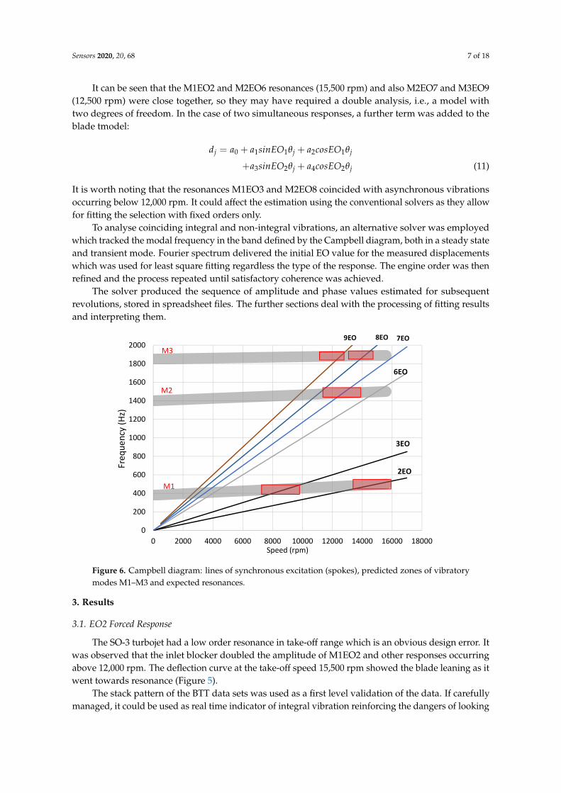
The approximate values of vibration frequency for selected modes and speeds were taken fromthe results of numerical modal analysis [39]. On the basis of this data, a Campbell diagram wasplotted, which was necessary to set up the solver (Figure 6). The observed resonances M1EO2, M1EO3,M2EO7 and M2EO8 were fitted in the so-called ’synchronous analysis’ with the integral engine order.The selection of resonances is limited by the available speed range (7200–15,500 rpm) and the set ofengine orders which is generated by the excitation force.

Sensors 2020, 20, 68 7 of 18

It can be seen that the M1EO2 and M2EO6 resonances (15,500 rpm) and also M2EO7 and M3EO9(12,500 rpm) were close together, so they may have required a double analysis, i.e., a model withtwo degrees of freedom. In the case of two simultaneous responses, a further term was added to theblade tmodel:

dj = a0 + a1sinEO1θj + a2cosEO1θj

+a3sinEO2θj + a4cosEO2θj (11)

It is worth noting that the resonances M1EO3 and M2EO8 coincided with asynchronous vibrationsoccurring below 12,000 rpm. It could affect the estimation using the conventional solvers as they allowfor fitting the selection with fixed orders only.

To analyse coinciding integral and non-integral vibrations, an alternative solver was employedwhich tracked the modal frequency in the band defined by the Campbell diagram, both in a steady stateand transient mode. Fourier spectrum delivered the initial EO value for the measured displacementswhich was used for least square fitting regardless the type of the response. The engine order was thenrefined and the process repeated until satisfactory coherence was achieved.

The solver produced the sequence of amplitude and phase values estimated for subsequentrevolutions, stored in spreadsheet files. The further sections deal with the processing of fitting resultsand interpreting them.

0

200

400

600

800

1000

1200

1400

1600

1800

2000

0 2000 4000 6000 8000 10000 12000 14000 16000 18000

Freq

uenc

y (H

z)

Speed (rpm)

7EO8EO9EO

6EO

3EO

2EO

M1

M2

M3

Figure 6. Campbell diagram: lines of synchronous excitation (spokes), predicted zones of vibratorymodes M1–M3 and expected resonances.

3. Results

3.1. EO2 Forced Response

The SO-3 turbojet had a low order resonance in take-off range which is an obvious design error. Itwas observed that the inlet blocker doubled the amplitude of M1EO2 and other responses occurringabove 12,000 rpm. The deflection curve at the take-off speed 15,500 rpm showed the blade leaning as itwent towards resonance (Figure 5).

The stack pattern of the BTT data sets was used as a first level validation of the data. If carefullymanaged, it could be used as real time indicator of integral vibration reinforcing the dangers of looking

Sensors 2020, 20, 68 8 of 18

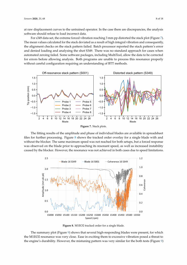
at raw displacement curves to the untrained operator. In the case there are discrepancies, the analysissoftware should refuse to load incorrect data.

For s349 data-set, the extreme forced vibration reaching 3 mm pp distorted the stack plot (Figure 7).The mean values calculated for the stack deviated as a result of high integral vibration and consequently,the alignment checks on the stack pattern failed. Batch processor reported the stack pattern’s errorand denied loading and analysing the shot S349. There was no standard approach for cases whenautomated zeroing failed. Some software packages, including MultiTool, allow the data to be correctedfor errors before allowing analysis. Both programs are unable to process this resonance properlywithout careful configuration requiring an understanding of BTT methods.

2 4 6 8 10 12 14 16 18 20 22 24 26Blade

1.5

1.0

0.5

0.0

0.5

1.0

1.5

Tip

posi

tion

(mm

)

Off-resonance stack pattern (S001)

Probe 1Probe 2Probe 3Probe 4

Probe 5Probe 6Probe 7Probe 8

2 4 6 8 10 12 14 16 18 20 22 24 26Blade

1.5

1.0

0.5

0.0

0.5

1.0

1.5

Distorted stack pattern (S349)

Figure 7. Stack plots.

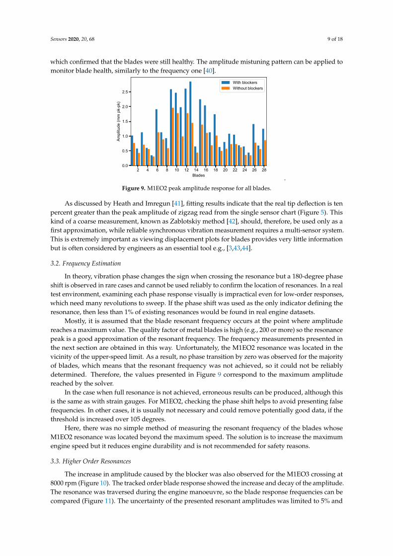
The fitting results of the amplitude and phase of individual blades are available in spreadsheetfiles for further processing. Figure 8 shows the tracked order overlay for a single blade with andwithout the blocker. The same maximum speed was not reached for both setups, but a forced responsewas observed on the blade prior to approaching its resonant speed, as well as increased instabilitycaused by the blocker. However, the resonance was not achieved in both cases due to speed limitations.

Figure 8. M1EO2 tracked order for a single blade.

The summary plot (Figure 9) shows that several high-responding blades were present, for whichthe M1EO2 resonance was very close. Ease in exciting them to excessive vibration posed a threat tothe engine’s durability. However, the mistuning pattern was very similar for the both tests (Figure 9)

Sensors 2020, 20, 68 9 of 18

which confirmed that the blades were still healthy. The amplitude mistuning pattern can be applied tomonitor blade health, similarly to the frequency one [40].

2 4 6 8 10 12 14 16 18 20 22 24 26 28Blades

0.0

0.5

1.0

1.5

2.0

2.5

Ampl

itude

(mm

pk-

pk)

With blockersWithout blockers

.Figure 9. M1EO2 peak amplitude response for all blades.

As discussed by Heath and Imregun [41], fitting results indicate that the real tip deflection is tenpercent greater than the peak amplitude of zigzag read from the single sensor chart (Figure 5). Thiskind of a coarse measurement, known as Zablotskiy method [42], should, therefore, be used only as afirst approximation, while reliable synchronous vibration measurement requires a multi-sensor system.This is extremely important as viewing displacement plots for blades provides very little informationbut is often considered by engineers as an essential tool e.g., [3,43,44].

3.2. Frequency Estimation

In theory, vibration phase changes the sign when crossing the resonance but a 180-degree phaseshift is observed in rare cases and cannot be used reliably to confirm the location of resonances. In a realtest environment, examining each phase response visually is impractical even for low-order responses,which need many revolutions to sweep. If the phase shift was used as the only indicator defining theresonance, then less than 1% of existing resonances would be found in real engine datasets.

Mostly, it is assumed that the blade resonant frequency occurs at the point where amplitudereaches a maximum value. The quality factor of metal blades is high (e.g., 200 or more) so the resonancepeak is a good approximation of the resonant frequency. The frequency measurements presented inthe next section are obtained in this way. Unfortunately, the M1EO2 resonance was located in thevicinity of the upper-speed limit. As a result, no phase transition by zero was observed for the majorityof blades, which means that the resonant frequency was not achieved, so it could not be reliablydetermined. Therefore, the values presented in Figure 9 correspond to the maximum amplitudereached by the solver.

In the case when full resonance is not achieved, erroneous results can be produced, although thisis the same as with strain gauges. For M1EO2, checking the phase shift helps to avoid presenting falsefrequencies. In other cases, it is usually not necessary and could remove potentially good data, if thethreshold is increased over 105 degrees.

Here, there was no simple method of measuring the resonant frequency of the blades whoseM1EO2 resonance was located beyond the maximum speed. The solution is to increase the maximumengine speed but it reduces engine durability and is not recommended for safety reasons.

3.3. Higher Order Resonances

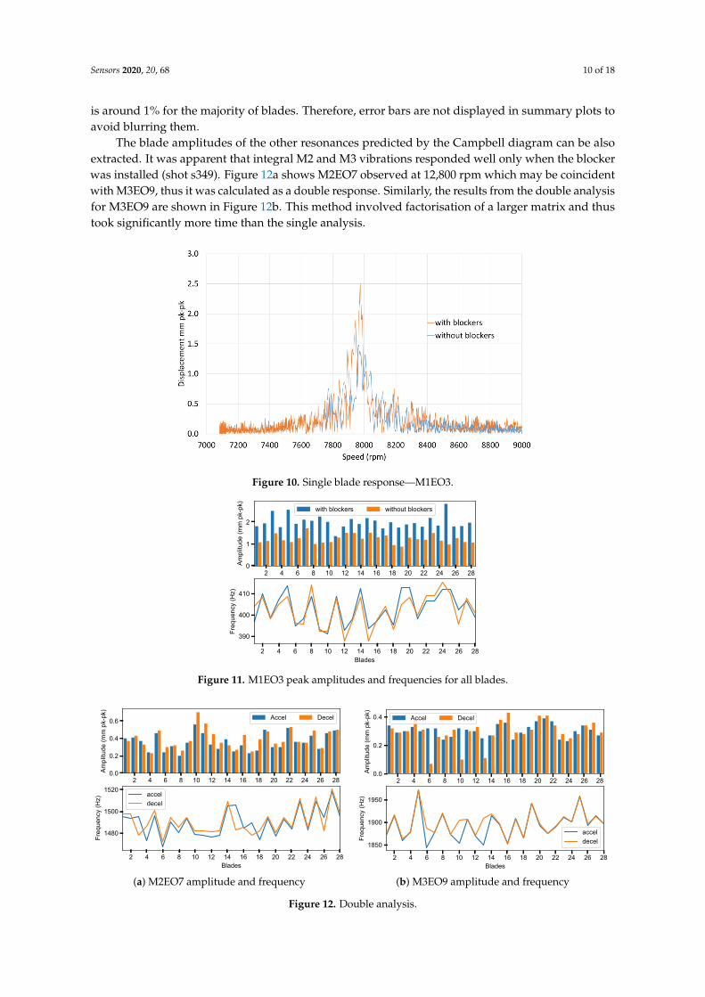
The increase in amplitude caused by the blocker was also observed for the M1EO3 crossing at8000 rpm (Figure 10). The tracked order blade response showed the increase and decay of the amplitude.The resonance was traversed during the engine manoeuvre, so the blade response frequencies can becompared (Figure 11). The uncertainty of the presented resonant amplitudes was limited to 5% and

Sensors 2020, 20, 68 10 of 18

is around 1% for the majority of blades. Therefore, error bars are not displayed in summary plots toavoid blurring them.

The blade amplitudes of the other resonances predicted by the Campbell diagram can be alsoextracted. It was apparent that integral M2 and M3 vibrations responded well only when the blockerwas installed (shot s349). Figure 12a shows M2EO7 observed at 12,800 rpm which may be coincidentwith M3EO9, thus it was calculated as a double response. Similarly, the results from the double analysisfor M3EO9 are shown in Figure 12b. This method involved factorisation of a larger matrix and thustook significantly more time than the single analysis.

Figure 10. Single blade response—M1EO3.

2 4 6 8 10 12 14 16 18 20 22 24 26 28Blades

0

1

2

Ampl

itude

(mm

pk-

pk)

with blockers without blockers

2 4 6 8 10 12 14 16 18 20 22 24 26 28Blades

390

400

410

Freq

uenc

y (H

z)

Figure 11. M1EO3 peak amplitudes and frequencies for all blades.

2 4 6 8 10 12 14 16 18 20 22 24 26 28Blades

0.0

0.2

0.4

0.6

Ampl

itude

(mm

pk-

pk)

Accel Decel

2 4 6 8 10 12 14 16 18 20 22 24 26 28Blades

1480

1500

1520

Freq

uenc

y (H

z)

acceldecel

(a) M2EO7 amplitude and frequency

2 4 6 8 10 12 14 16 18 20 22 24 26 28Blades

0.0

0.2

0.4

Ampl

itude

(mm

pk-

pk)

Accel Decel

2 4 6 8 10 12 14 16 18 20 22 24 26 28Blades

1850

1900

1950

Freq

uenc

y (H

z)

acceldecel

(b) M3EO9 amplitude and frequency

Figure 12. Double analysis.

Sensors 2020, 20, 68 11 of 18

Observing the responses and overlaying them on a common speed time base (Figure 13) indicatesthat the two modes were not really coupled and could have been analysed as single responses.

Figure 13. M2 and M3 overlay shows no coupling.

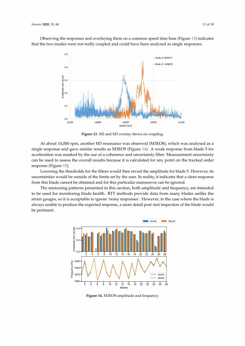
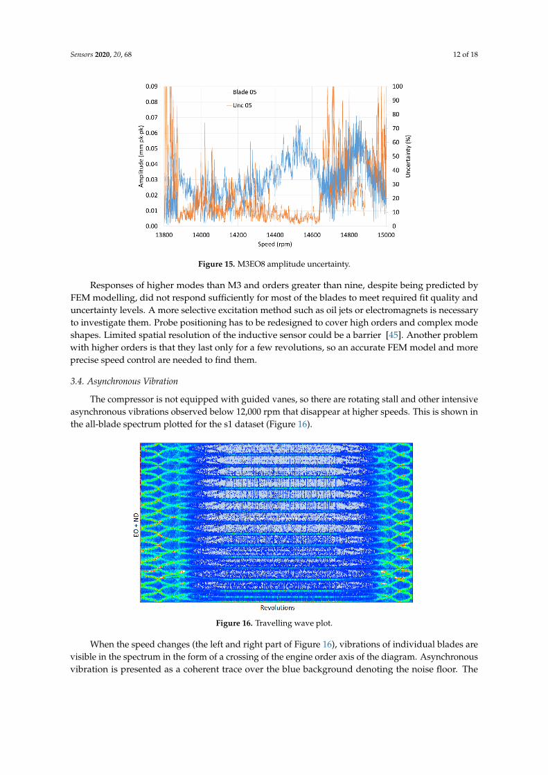
At about 14,000 rpm, another M3 resonance was observed (M3EO8), which was analysed as asingle response and gave similar results as M3EO9 (Figure 14). A weak response from blade 5 foracceleration was masked by the use of a coherence and uncertainty filter. Measurement uncertaintycan be used to assess the overall results because it is calculated for any point on the tracked orderresponse (Figure 15).

Lowering the thresholds for the filters would then reveal the amplitude for blade 5. However, itsuncertainties would be outside of the limits set by the user. In reality, it indicates that a clean responsefrom this blade cannot be obtained and for this particular manoeuvre can be ignored.

The mistuning patterns presented in this section, both amplitude and frequency, are intendedto be used for monitoring blade health. BTT methods provide data from many blades unlike thestrain gauges, so it is acceptable to ignore ‘noisy responses’. However, in the case where the blade isalways unable to produce the expected response, a more detail post–test inspection of the blade wouldbe pertinent.

2 4 6 8 10 12 14 16 18 20 22 24 26 28Blades

0.0

0.2

0.4

Ampl

itude

(mm

pk-

pk)

2 4 6 8 10 12 14 16 18 20 22 24 26 28Blades

1850

1875

1900

1925

Freq

uenc

y (H

z)

acceldecel

Accel Decel

Figure 14. M3EO8 amplitude and frequency.

Sensors 2020, 20, 68 12 of 18

Figure 15. M3EO8 amplitude uncertainty.

Responses of higher modes than M3 and orders greater than nine, despite being predicted byFEM modelling, did not respond sufficiently for most of the blades to meet required fit quality anduncertainty levels. A more selective excitation method such as oil jets or electromagnets is necessaryto investigate them. Probe positioning has to be redesigned to cover high orders and complex modeshapes. Limited spatial resolution of the inductive sensor could be a barrier [45]. Another problemwith higher orders is that they last only for a few revolutions, so an accurate FEM model and moreprecise speed control are needed to find them.

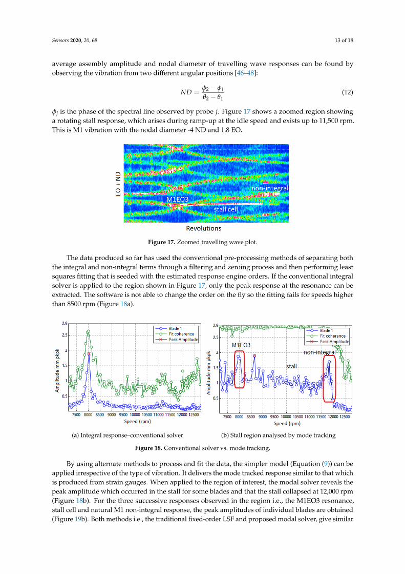
3.4. Asynchronous Vibration

The compressor is not equipped with guided vanes, so there are rotating stall and other intensiveasynchronous vibrations observed below 12,000 rpm that disappear at higher speeds. This is shown inthe all-blade spectrum plotted for the s1 dataset (Figure 16).

Figure 16. Travelling wave plot.

When the speed changes (the left and right part of Figure 16), vibrations of individual blades arevisible in the spectrum in the form of a crossing of the engine order axis of the diagram. Asynchronousvibration is presented as a coherent trace over the blue background denoting the noise floor. The

Sensors 2020, 20, 68 13 of 18

average assembly amplitude and nodal diameter of travelling wave responses can be found byobserving the vibration from two different angular positions [46–48]:

ND =φ2 − φ1

θ2 − θ1(12)

φj is the phase of the spectral line observed by probe j. Figure 17 shows a zoomed region showinga rotating stall response, which arises during ramp-up at the idle speed and exists up to 11,500 rpm.This is M1 vibration with the nodal diameter -4 ND and 1.8 EO.

Figure 17. Zoomed travelling wave plot.

The data produced so far has used the conventional pre-processing methods of separating boththe integral and non-integral terms through a filtering and zeroing process and then performing leastsquares fitting that is seeded with the estimated response engine orders. If the conventional integralsolver is applied to the region shown in Figure 17, only the peak response at the resonance can beextracted. The software is not able to change the order on the fly so the fitting fails for speeds higherthan 8500 rpm (Figure 18a).

(a) Integral response–conventional solver (b) Stall region analysed by mode tracking

Figure 18. Conventional solver vs. mode tracking.

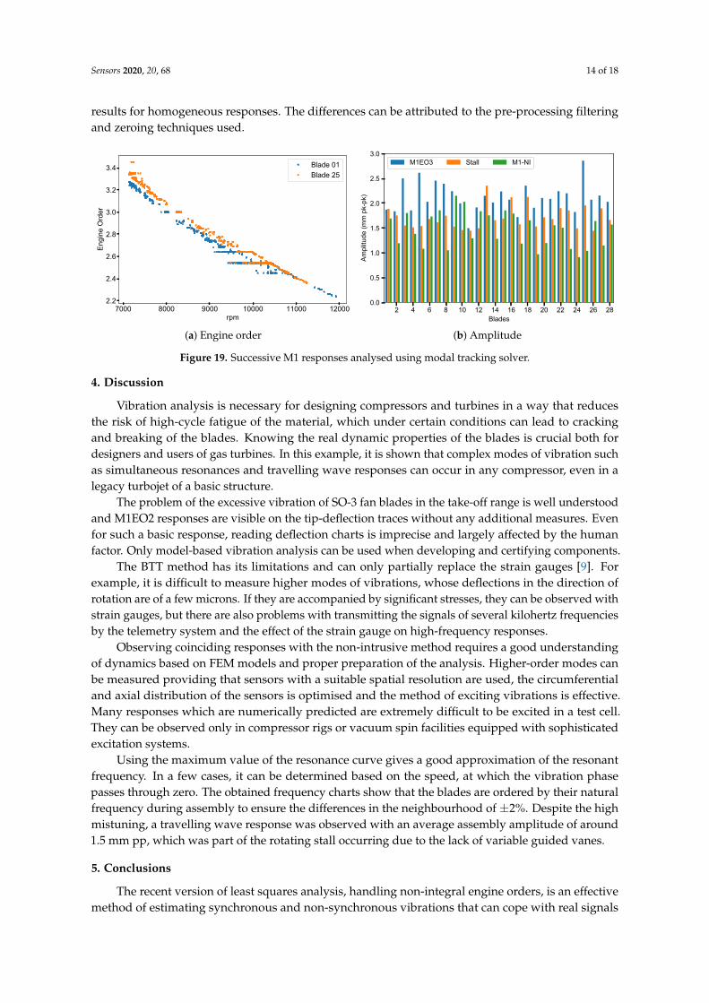
By using alternate methods to process and fit the data, the simpler model (Equation (9)) can beapplied irrespective of the type of vibration. It delivers the mode tracked response similar to that whichis produced from strain gauges. When applied to the region of interest, the modal solver reveals thepeak amplitude which occurred in the stall for some blades and that the stall collapsed at 12,000 rpm(Figure 18b). For the three successive responses observed in the region i.e., the M1EO3 resonance,stall cell and natural M1 non-integral response, the peak amplitudes of individual blades are obtained(Figure 19b). Both methods i.e., the traditional fixed-order LSF and proposed modal solver, give similar

Sensors 2020, 20, 68 14 of 18

results for homogeneous responses. The differences can be attributed to the pre-processing filteringand zeroing techniques used.

7000 8000 9000 10000 11000 12000rpm

2.2

2.4

2.6

2.8

3.0

3.2

3.4

Engi

ne O

rder

Blade 01Blade 25

(a) Engine order

2 4 6 8 10 12 14 16 18 20 22 24 26 28Blades

0.0

0.5

1.0

1.5

2.0

2.5

3.0

Ampl

itude

(mm

pk-

pk)

M1EO3 Stall M1-NI

(b) Amplitude

Figure 19. Successive M1 responses analysed using modal tracking solver.

4. Discussion

Vibration analysis is necessary for designing compressors and turbines in a way that reducesthe risk of high-cycle fatigue of the material, which under certain conditions can lead to crackingand breaking of the blades. Knowing the real dynamic properties of the blades is crucial both fordesigners and users of gas turbines. In this example, it is shown that complex modes of vibration suchas simultaneous resonances and travelling wave responses can occur in any compressor, even in alegacy turbojet of a basic structure.

The problem of the excessive vibration of SO-3 fan blades in the take-off range is well understoodand M1EO2 responses are visible on the tip-deflection traces without any additional measures. Evenfor such a basic response, reading deflection charts is imprecise and largely affected by the humanfactor. Only model-based vibration analysis can be used when developing and certifying components.

The BTT method has its limitations and can only partially replace the strain gauges [9]. Forexample, it is difficult to measure higher modes of vibrations, whose deflections in the direction ofrotation are of a few microns. If they are accompanied by significant stresses, they can be observed withstrain gauges, but there are also problems with transmitting the signals of several kilohertz frequenciesby the telemetry system and the effect of the strain gauge on high-frequency responses.

Observing coinciding responses with the non-intrusive method requires a good understandingof dynamics based on FEM models and proper preparation of the analysis. Higher-order modes canbe measured providing that sensors with a suitable spatial resolution are used, the circumferentialand axial distribution of the sensors is optimised and the method of exciting vibrations is effective.Many responses which are numerically predicted are extremely difficult to be excited in a test cell.They can be observed only in compressor rigs or vacuum spin facilities equipped with sophisticatedexcitation systems.

Using the maximum value of the resonance curve gives a good approximation of the resonantfrequency. In a few cases, it can be determined based on the speed, at which the vibration phasepasses through zero. The obtained frequency charts show that the blades are ordered by their naturalfrequency during assembly to ensure the differences in the neighbourhood of ±2%. Despite the highmistuning, a travelling wave response was observed with an average assembly amplitude of around1.5 mm pp, which was part of the rotating stall occurring due to the lack of variable guided vanes.

5. Conclusions

The recent version of least squares analysis, handling non-integral engine orders, is an effectivemethod of estimating synchronous and non-synchronous vibrations that can cope with real signals

Sensors 2020, 20, 68 15 of 18

including noise. The presented solver can track the modal frequency and adjust the engine orderon the fly. The obtained results are constantly evaluated by monitoring coherence and uncertainty.This procedure let us analyse the three close M1 responses (integral, stall and non-integral) in onego and saved a lot of the tedious work configuring the conventional solver, in which the integer andnon-integer responses are treated separately. By using the same method for both types of vibration,it was possible to examine the interaction between the rotating stall and the M1EO3 resonance. Thisgeneralised approach to blade vibration analysis and uncertainty estimation is an important steptowards replacing strain gauges in engine certification.

Author Contributions: Conceptualization, R.P.; methodology, R.P. and P.R.; formal analysis, R.P. and P.R.;software, R.P. and P.R.; validation, R.P. and P.R.; investigation, R.P.; resources, R.P.; writing—original draftpreparation, R.P.; writing—review and editing, R.P. and P.R.; visualization R.P. and P.R. All authors have read andagreed to the published version of the manuscript.

Funding: This publication includes the results of the project financed by the Polish National Science Centre(NCN) under the decision DEC-2011/01/D/ST8/07612 and the research task of the statutory activity of ITWL’Demonstrator of the system to measure turbine blade vibration’, financed by the Ministry of Science and HigherEducation in 2018–2019.

Acknowledgments: We would like to thank Michał Wachłaczenko and Wojciech Sujka for their involvement inthe project and support for engine tests.

Conflicts of Interest: The authors declare no conflict of interest.

Abbreviations

The following symbols and abbreviations are used in this manuscript:

φj phase observed by probe jθj angular position of probe jA blade vibration amplitudedj blade displacement measured by probe jf eo fractional engine orderH number of revolutionsh revolution numberi blade numberj probe numberN number of bladesM number of probesPj invariant offset for probe jpk-pk peak-to-peak amplituder Pearson correlation coefficient (coherence)rpm revolutions per minuteunc uncertaintyBHM Blade Health MonitoringBTT Blade Tip-TimingEO Engine OrderFEM Finite Element MethodFFT Fast Fourier TransformIGV Inlet Guide VanesITWL Air Force Institute of Technology in WarsawLSF Least Squares FittingM1 1st vibration modeMDPI Multidisciplinary Digital Publishing InstituteND nodal diameterNI non-integral vibrationsNSMS Non-contact Stress Measurement System

Sensors 2020, 20, 68 16 of 18

References

1. Russhard, P. The Rise and Fall of the Rotor Blade Strain Gauge. In Vibration Engineering and Technology ofMachinery; Mechanisms and Machine Science; Sinha, J.K., Ed.; Springer International Publishing: Cham,Switzerland, 2015; Volume 23, pp. 27–38. [CrossRef]

2. Mevissen, F.; Meo, M. A Review of NDT/Structural Health Monitoring Techniques for Hot Gas Componentsin Gas Turbines. Sensors 2019, 19, 711. [CrossRef]

3. Zhao, X.; Zhou, Q.; Yang, S.; Li, H. Rotating Stall Induced Non-Synchronous Blade. Sensors 2019, 19, 4995.[CrossRef]

4. Ye, D.; Duan, F.; Jiang, J.; Cheng, Z.; Niu, G.; Shan, P.; Zhang, J. Synchronous vibration measurementsfor shrouded blades based on fiber optical sensors with lenses in a steam turbine. Sensors 2019, 19, 2501.[CrossRef]

5. Agilis Non-Intrusive Stress Measurement Systems Fundamentals; Technical Report; Agilis Measurement Systems:Palm Beach Gardens, FL, USA, 2014.

6. Tappert, P.; Losh, D. Analyze Blade Vibration 6.1 User Manual; Technical Report; Hood Technology Corporation:Hood River, OR, USA, 2007.

7. Jousselin, O. Development of Blade Tip Timing Techniques in Turbo Machinery. Ph.D. Thesis, The Universityof Manchester, Manchester, UK, 2013.

8. Russhard, P. Analysis of Rotating Stall in a Contra-Rotating System using Blade Tip Timing. In Proceedingsof the 58th International Instrumentation Symposium, San Diego, CA, USA, 4–8 June 2012; pp. 1–33.

9. Knappett, D.; Garcia, J. Blade tip timing and strain gauge correlation on compressor blades. Proc. Inst. Mech.Eng. Part G J. Aerosp. Eng. 2008, 222, 497–506. [CrossRef]

10. Przysowa, R. The Analysis Of Synchronous Blade Vibration Using Linear Sine Fitting. J. Konbin 2014,30, 5–19. [CrossRef]

11. Dimitriadis, G.; Carrington, I.; Wright, J.; Cooper, J. Blade-Tip Timing measurement of SynchronousVibrations of Rotating Blade assemblies. Mech. Syst. Signal Process. 2002, 16, 599–622. [CrossRef]

12. Beauseroy, P.; Lengellé, R. Nonintrusive turbomachine blade vibration measurement system. Mech. Syst.Signal Process. 2007, 21, 1717–1738. [CrossRef]

13. Teolis, C.; Teolis, A.; Paduano, J.; Lackner, M. Analytic representation of eddy current sensor data for faultdiagnostics. In Proceedings of the 2005 IEEE Aerospace Conference, Big Sky, MT, USA, 5–12 March 2005;pp. 1–11. [CrossRef]

14. Li, M.; Duan, F.; Ouyang, T. Analysis of blade vibration frequencies from blade tip timing data. Proc. SPIE2010, 7544, 7544–7544F. [CrossRef]

15. Diamond, D.H.; Heyns, P.S.; Oberholster, A.J. A Comparison Between Three Blade Tip Timing Algorithmsfor Estimating Synchronous Turbomachine Blade Vibration. In Proceedings of the 9th WCEAM 2014 WorldCongress on Engineering Asset Management; Lecture Notes in Mechanical Engineering; Amadi-Echendu, J.,Hoohlo, C., Mathew, J., Eds.; Springer International Publishing: Cham, Switzerland, 2015; Volume 20,pp. 215–225. [CrossRef]

16. Kharyton, V.; Dimitriadis, G.; Defise, C. A Discussion on the Advancement of Blade Tip Timing DataProcessing. In Proceedings of the ASME Turbo Expo 2017: Turbomachinery Technical Conference andExposition, Charlotte, NC, USA, 26–30 June 2017. [CrossRef]

17. Bastami, A.R.; Safarpour, P.; Mikaeily, A.; Mohammadi, M. Identification of Asynchronous Blade VibrationParameters by Linear Regression of Blade Tip Timing Data. J. Eng. Gas Turbines Power 2018, 140, 072506.[CrossRef]

18. Zhang, J.W.; Zhang, L.B.; Duan, L.X. A Blade Defect Diagnosis Method by Fusing Blade Tip Timing and TipClearance Information. Sensors 2018, 18, 2166. [CrossRef] [PubMed]

19. Hu, Z.; Lin, J.; Chen, Z.S.; Yang, Y.M.; Li, X.J. A non-uniformly under-sampled blade tip-timing signalreconstruction method for blade vibration monitoring. Sensors 2015, 15, 2419–2437. [CrossRef] [PubMed]

20. Chen, Z.; Liu, J.; Zhan, C.; He, J.; Wang, W. Reconstructed order analysis-based vibration monitoring undervariable rotation speed by using multiple blade tip-timing sensors. Sensors 2018, 18, 3235. [CrossRef][PubMed]

Sensors 2020, 20, 68 17 of 18

21. Pan, M.; Yang, Y.; Guan, F.; Hu, H.; Xu, H. Sparse Representation Based Frequency Detection and UncertaintyReduction in Blade Tip Timing Measurement for Multi-Mode Blade Vibration Monitoring. Sensors 2017,17, 1745. [CrossRef]

22. Jousselin, O.; Russhard, P.; Bonello, P. A method for establishing the uncertainty levels for aero-engine bladetip amplitudes extracted from blade tip timing data. In Proceedings of the 10th International Conference onVibrations in Rotating Machinery, London, UK, 11–13 September 2012; pp. 211–220.[CrossRef]

23. Courtney, S. A Robust Process for the Certification of Rotating Components Using Blade Tip TimingMeasurements z. In Proceedings of the ISA 57th IIS 2nd Tip Timing Workshop; The International Society ofAutomation: St. Louis, MO, USA, 2011.

24. Drewczynski, M.; Rzadkowski, R.; Ostrowska, Z. Dynamic Stress Analysis of a Blade in a Partially BlockedEngine Inlet. In Proceedings of the ASME Turbo Expo 2014: Turbine Technical Conference and Exposition.Volume 7B: Structures and Dynamics, Düsseldorf, Germany, 16–20 June 2014.[CrossRef]

25. Morris, R.; Littles, J.W.; Hall, B.; Owen, W.D.; Tulpule, S.; Szczepanik, R.; Przysowa, R. Crack Detectionand Prognosis Using Non-Contact Time of Arrival Sensors for Fan and Compressor Airfoils In Gas TurbineEngines. In Proceedings of the 20th Advanced Aerospace Materials and Processes (AeroMat) Conference andExposition; ASM International: Dayton, OH, USA, 2009; pp. 1–26.

26. Witos, M. High sensitive methods for health monitoring of compressor blades and fatigue detection. Sci.World J. 2013, 2013. [CrossRef] [PubMed]

27. Szczepanik, R. Experimental Investigations of Aircraft Engine Rotor Blade Dynamics; Wydawnictwo InstytutuTechnicznego Wojsk Lotniczych: Warsaw, Poland, 2013.

28. Przysowa, R.; Kazmierczak, K. Triggering methods in blade tip-timing systems. In Proceedings of the TwelveInternational Conference on Vibration Engineering and Technology of Machinery, VETOMAC XII; Rzadkowski, R.,Szczepanik, R., Eds.; Instytut Techniczny Wojsk Lotniczych: Warsaw, Poland, 2016; pp. 129–138. [CrossRef]

29. Przysowa, R.; Tuzik, A. Data Management Techniques for Blade Vibration Analysis. J. Konbin 2016,37, 95–132. [CrossRef]

30. Mohamed, M.; Bonello, P.; Russhard, P. A Novel Method for the Determination of The Change in Blade TipTiming Probe Sensing Position Due to Steady Movements. Mech. Syst. Signal Process. 2019, 126, 686–710.[CrossRef]

31. Russhard, P.; Back, J.D. Rotating Blade Analysis. U.S. Patent 9,016,132, 28 April 2015.32. Ye, D.; Duan, F.; Jiang, J.; Niu, G.; Liu, Z.; Li, F. Identification of vibration events in rotating blades using a

fiber optical tip timing sensor. Sensors 2019, 19, 1482. [CrossRef]33. Russhard, P. BTT Data Zeroing Techniques. In Proceedings of the 59th International Instrumentation Symposium

and 2013 MFPT Conference; The International Society of Automation: Cleveland, OH, USA, 2013; pp. 1–46.34. Jousselin, O. Blade Tip Timing Batch Processor User Guide DNS147027; Technical Report; Rolls-Royce plc:

Derby, UK, 2010.35. Russhard, P. MultiTool Blade Tip Timing Acquisition, Analysis and Data Simulation Software; EM0102–Analysis

Manual; Technical Report; EMTD Ltd.: Nottingham, UK, 2016.36. Russhard, P. Blade tip timing (BTT) uncertainties. AIP Conf. Proc. 2016, 1740, 020003. [CrossRef]37. Sinha, S.K.; Turner, K.E. Natural frequencies of a pre-twisted blade in a centrifugal force field. J. Sound Vib.

2011, 330, 2655–2681. [CrossRef]38. Chakshu, N.K.; Sinha, S.K. Natural Frequencies of Pre-Twisted Airfoil Blades. In Proceedings of the

ASME 2017 Gas Turbine India Conference. Volume 2: Structures and Dynamics; Renewable Energy(Solar, Wind); Inlets and Exhausts; Emerging Technologies (Hybrid Electric Propulsion, UAV, ...); GTOperation and Maintenance; Materials and Manufacturing (Including Coatings, Composites, CMCs,Additive Manufacturing); Analytics and Digital Solutions for Gas Turbines/Rotating Machinery, Bangalore,India, 7–8 December 2017. [CrossRef]

39. Rzadkowski, R.; Szczepanik, R.; Drewczynski, M. Analiza dynamiczna łopatek wirnikowych i kierowniczychsilnika jednoprzepływowego (Dynamic analysis of turbojet’s blades and vanes); ITWL: Warsaw, Poland, 2013.

Sensors 2020, 20, 68 18 of 18

40. Russhard, P. The Use of Blade Tip Timing Technologies to Assess and Monitor Rotor Blade Health fromDesign to Production. In STO-MP-AVT-229—Test Cell and Controls Instrumentation and EHM Technologies forMilitary Air, Land and Sea Turbine Engines; NATO Science and Technology Organization: Rzeszow, Poland,2015; Chapter 11, pp. 1–27.

41. Heath, S.; Imregun, M. An improved single-parameter tip-timing method for turbomachinery blade vibrationmeasurements using optical laser probes. Int. J. Mech. Sci. 1996, 38, 1047–1058. [CrossRef]

42. Zablotskiy, I.Y.; Korostelev, Y.A.; Sviblov, L.B. Contactless Measuring of Vibrations in the Rotor Blades ofTurbines; FTD-HT-23-673-74; Lopatochnyye Mashiny i Struynyye Apparaty; Foreign Technology Div:Wright-Patterson AFB, OH, USA, 1972; pp. 106–121.

43. Zhang, J.; Duan, F.; Niu, G.; Jiang, J.; Li, J. A blade tip timing method based on a microwave sensor. Sensors2017, 17, 1097. [CrossRef] [PubMed]

44. Gil-García, J.M.; Solís, A.; Aranguren, G.; Zubia, J. An architecture for On-Line measurement of the tipclearance and time of arrival of a bladed disk of an aircraft engine. Sensors 2017, 17, 2162. [CrossRef][PubMed]

45. Russhard, P. A Comparison of Multi Fibre and Single Fibre Optical Probes. In Proceedings of the 60thInternational Instrumentation Symposium and IET Conference, London, UK, 24–26 June 2014; pp. 1–5.[CrossRef]

46. Watkins, W.B.; Chi, R.M. Noninterference blade-vibration measurement system for gas turbine engines.J. Propuls. Power 1989, 5, 727–730. [CrossRef]

47. Gill, J.D.; Capece, V.R.; Fost, R.B. Experimental methods applied in a study of stall flutter in an axial flowfan. Shock Vib. 2004, 11, 597–613. [CrossRef]

48. García, I.; Beloki, J.; Zubia, J.; Aldabaldetreku, G.; Asunción Illarramendi, M.; Jiménez, F. An optical fiberbundle sensor for tip clearance and tip timing measurements in a turbine rig. Sensors 2013, 13, 7385–7398.[CrossRef]

c© 2019 by the authors. Licensee MDPI, Basel, Switzerland. This article is an open accessarticle distributed under the terms and conditions of the Creative Commons Attribution(CC BY) license (http://creativecommons.org/licenses/by/4.0/).