Embed Size (px)
Citation preview

On the Interaction of Elastic Waves with
Buried Land Mines: an Investigation Using
the Finite-Di�erence Time-Domain Method
A Thesis
Presented to
The Academic Faculty
by
Christoph T. Schr�oder
In Partial Ful�llment
of the Requirements for the Degree of
Doctor of Philosophy in Electrical and Computer Engineering
Georgia Institute of Technology
July 2001

On the Interaction of Elastic Waves with Buried
Land Mines: an Investigation Using the
Finite-Di�erence Time-Domain Method
Approved:
Waymond R. Scott, Jr., Chairman
Glenn S. Smith
Andrew F. Peterson
W. Marshall Leach
Peter H. Rogers
Date Approved
ii

ACKNOWLEDGMENTS
This dissertation is the result of my studies at the Georgia Institute of Technology
between the fall of 1996 and the summer of 2001. Many people have, in one way or
the other, contributed to this work, and I am grateful to all of them.
I owe my deepest gratitude to Prof. Waymond R. Scott, Jr., who served as my
thesis advisor and has guided my way at Georgia Tech from the very �rst moments.
His expertise in both electromagnetics and elasticity, his curiosity and his interest
have taught me, have kept my spirit up through all these years and have made my
work truly worthwhile.
I wish to thank the members of my dissertation committee, Prof. Glenn S. Smith,
Prof. Andrew F. Peterson, Prof. W. Marshall Leach, and Prof. Peter. H. Rogers,
together with Prof. Scott, for their time, e�ort, and constructive criticism. I am
especially grateful to Prof. Smith, who inspired me with his vast knowledge in elec-
tromagnetics and his understanding of wave propagation. He always had an open ear
for discussions of any kind, making long hours at school enjoyable.
Dr. Gregg D. Larson and James S. Martin, together with Prof. Scott, have
developed the elastic/electromagntic sensor system. They performed numerous mea-
surements speci�cally for this work, results of which will be shown within this text.
Their insight and knowledge of elasticity were extremely helpful.
Benny Venkatesan has built and administered the Beowulf computer cluster
that was used for most of the computations in this work. The cluster proved to be
invaluable providing the computational resources required for this work.
My parents, Detlef and Hannelore Schr�oder, and my brother, Achim Schr�oder,
iii
ACKNOWLEDGMENTS
have lovingly supported me throughout these years. Without their help and encour-
agement nothing of this would have been possible. I regret having been parted from
them for so long, and look forward to being closer to them in the future.
I furthermore want to express my gratitude to the many friends I have found
during my time in Atlanta. Padma Rao has been closest to me, and I am grateful for
her friendship and her faith in me. Thorsten Hertel has known me the longest, and
has come a long way with me since we started our studies in the city of Braunschweig
in Germany in 1993. I appreciate his friendship and his kind helpfulness. I would also
like to thank Peter Knobel, Stefan Galler and Harald Seckel for being good friends
and the World Student Fund, skillfully and warmly steered by Carlton Parker, for
providing the opportunity for so many international students to study in the United
States.
This work has been supported in part under the OSD MURI program by the
US Army Research OÆce under contract DAAH04-96-1-0448, by a grant from the
US OÆce of Naval Research under contract N00014-99-1-0995, and by an equipment
grant from the Intel Corporation.
iv

Contents
ACKNOWLEDGMENTS ii
LIST OF TABLES ix
LIST OF FIGURES x
SUMMARY xv
1 Introduction 1
2 Background 5
3 Elastic Wave Propagation in Solids 10
3.1 Governing Equations . . . . . . . . . . . . . . . . . . . . . . . . . . . 10
3.2 Elastic Waves in Isotropic Media . . . . . . . . . . . . . . . . . . . . 13
3.2.1 The Wave Equation in Isotropic Media . . . . . . . . . . . . . . 13
3.2.2 Propagating Waves . . . . . . . . . . . . . . . . . . . . . . . . . 14
4 Numerical Model 18
4.1 The Finite-Di�erence Scheme . . . . . . . . . . . . . . . . . . . . . . 18
4.1.1 Problem Statement . . . . . . . . . . . . . . . . . . . . . . . . . 18
4.1.2 Governing Equations . . . . . . . . . . . . . . . . . . . . . . . . 20
4.1.3 Discretization of the Governing Equations . . . . . . . . . . . . 23
4.2 Boundaries . . . . . . . . . . . . . . . . . . . . . . . . . . . . . . . . 30
v

CONTENTS
4.2.1 Source . . . . . . . . . . . . . . . . . . . . . . . . . . . . . . . . 30
4.2.2 Internal Boundaries . . . . . . . . . . . . . . . . . . . . . . . . . 30
4.2.3 Free-Surface Boundary . . . . . . . . . . . . . . . . . . . . . . . 32
4.2.4 Perfectly-Matched Layer Absorbing Boundary . . . . . . . . . . 36
4.3 Injection of Plane Waves . . . . . . . . . . . . . . . . . . . . . . . . . 39
4.3.1 Procedure . . . . . . . . . . . . . . . . . . . . . . . . . . . . . . 41
4.3.2 Incident Field . . . . . . . . . . . . . . . . . . . . . . . . . . . . 44
4.4 Parallelization . . . . . . . . . . . . . . . . . . . . . . . . . . . . . . . 45
5 Stability of the FDTD Algorithm at a Material Interface 47
5.1 Stability Analysis: Theory . . . . . . . . . . . . . . . . . . . . . . . . 48
5.1.1 1-D Longitudinal Wave Incident onto a Material Interface . . . . 49
5.2 Stability Analysis: Numerical Results . . . . . . . . . . . . . . . . . . 61
5.2.1 1-D Case . . . . . . . . . . . . . . . . . . . . . . . . . . . . . . . 61
5.2.2 2-D Case . . . . . . . . . . . . . . . . . . . . . . . . . . . . . . . 67
5.3 Averaging . . . . . . . . . . . . . . . . . . . . . . . . . . . . . . . . . 71
5.3.1 Material Density . . . . . . . . . . . . . . . . . . . . . . . . . . 74
5.3.2 Lam�e's Constants . . . . . . . . . . . . . . . . . . . . . . . . . . 77
5.4 The Courant Condition . . . . . . . . . . . . . . . . . . . . . . . . . 79
5.5 Concluding Remarks . . . . . . . . . . . . . . . . . . . . . . . . . . . 80
6 Elastic Surface Waves 81
6.1 The Rayleigh Equation . . . . . . . . . . . . . . . . . . . . . . . . . . 82
6.2 The Roots of the Rayleigh Equation . . . . . . . . . . . . . . . . . . 86
6.2.1 Materials with a Poisson Ratio larger than 0.263 . . . . . . . . . 87
6.2.2 Materials with a Poisson Ratio smaller than 0.263 . . . . . . . . 95
6.3 Waves due to a Line Source on the Surface . . . . . . . . . . . . . . . 101
6.3.1 General Considerations . . . . . . . . . . . . . . . . . . . . . . . 103
6.3.2 Steepest-Descent Approximation . . . . . . . . . . . . . . . . . 106
6.3.3 Example . . . . . . . . . . . . . . . . . . . . . . . . . . . . . . . 114
vi
CONTENTS
7 Propagation and Scattering of Elastic Waves in the Ground 120
7.1 Surface Waves . . . . . . . . . . . . . . . . . . . . . . . . . . . . . . . 124
7.2 Interaction of Elastic Waves with Buried Land Mines . . . . . . . . . 133
7.2.1 2-D Analysis . . . . . . . . . . . . . . . . . . . . . . . . . . . . . 135
7.2.2 3-D Analysis . . . . . . . . . . . . . . . . . . . . . . . . . . . . . 142
7.3 Mines in the Presence of Clutter . . . . . . . . . . . . . . . . . . . . 151
7.4 A Moving-Source/Moving-Receiver System . . . . . . . . . . . . . . . 155
8 Modeling of Resonant Structures: the Resonance Behavior of a
Buried Land Mine 162
8.1 Discretization of Elastic Objects . . . . . . . . . . . . . . . . . . . . . 163
8.1.1 Long Thin Bar . . . . . . . . . . . . . . . . . . . . . . . . . . . 163
8.1.2 Thin Circular Plate . . . . . . . . . . . . . . . . . . . . . . . . . 167
8.1.3 Tuning Fork . . . . . . . . . . . . . . . . . . . . . . . . . . . . . 170
8.2 Resonance Behavior of a Buried Land Mine . . . . . . . . . . . . . . 174
8.3 Excitation by a Pressure Wave . . . . . . . . . . . . . . . . . . . . . 185
9 Experiments 191
9.1 Measuring the Water Content in the Ground . . . . . . . . . . . . . . 192
9.2 Measuring the Wave Speeds in the Ground . . . . . . . . . . . . . . . 196
9.2.1 Experimental Set-Up . . . . . . . . . . . . . . . . . . . . . . . . 197
9.2.2 Measurement Procedure . . . . . . . . . . . . . . . . . . . . . . 199
9.2.3 Results . . . . . . . . . . . . . . . . . . . . . . . . . . . . . . . . 203
9.3 Measurements of the Mine-Wave Interaction . . . . . . . . . . . . . . 215
10 Summary and Conclusions 217
APPENDIX A 3-D FDTD Equations 221
APPENDIX B Total-Field/Scattered-Field Formulation: Correction
Terms 226
vii
CONTENTS
APPENDIX C Software Documentation 229
C.1 Input File . . . . . . . . . . . . . . . . . . . . . . . . . 230
C.1.1 General Simulation Parameters . . . . . . . . . . 230
C.1.2 Sources . . . . . . . . . . . . . . . . . . . . . . . 232
C.1.3 Objects . . . . . . . . . . . . . . . . . . . . . . . 234
C.1.4 Background . . . . . . . . . . . . . . . . . . . . . 236
C.1.5 Materials . . . . . . . . . . . . . . . . . . . . . . 237
C.1.6 Sample Input File . . . . . . . . . . . . . . . . . 237
APPENDIX D Elastic Constants for Isotropic Solids 239
BIBLIOGRAPHY 240
VITA 247
viii

List of Tables
4.1 Positions of the �eld components of the (i; j; k)-th cell in the �nite-di�erence grid. . . . . . . . . . . . . . . . . . . . . . . . . . . . . . . 27
6.1 Solutions to the Rayleigh equation for � > 0:263. . . . . . . . . . . . 896.2 Solutions to the Rayleigh equation for � = 0:4: wave numbers. . . . . 906.3 Solutions to the Rayleigh equation for � < 0:263. . . . . . . . . . . . 1006.4 Solutions to the Rayleigh equation for � = 0:2: wave numbers. . . . . 101
7.1 Material properties. . . . . . . . . . . . . . . . . . . . . . . . . . . . . 121
8.1 Wave numbers and wave length of the �rst two harmonics of a barwith free ends according to the Bernoulli-Euler theory. . . . . . . . . 164
8.2 Resonant frequencies of a long thin bar. . . . . . . . . . . . . . . . . 1658.3 Resonant frequencies of the �rst three modes of a thin circular disc
that is free along its edge. . . . . . . . . . . . . . . . . . . . . . . . . 1698.4 Resonant frequencies of the thin circular plate as computed with the
numerical model. . . . . . . . . . . . . . . . . . . . . . . . . . . . . . 1698.5 Resonant frequencies of a tuning fork. . . . . . . . . . . . . . . . . . 1728.6 Material properties of the parts of the detailed mine model. . . . . . 174
9.1 Measurement of the water content as a function of depth. . . . . . . . 1949.2 Measured arrival times and wave speeds: pressure wave front. . . . . 205
B.1 Field components and correction terms at Interface I and II. . . . . . 227B.2 Field components and correction terms at Interface III and IV. . . . . 228B.3 Field components and correction terms at Interface V and VI . . . . . 228
ix

List of Figures
1.1 Schematic drawing of the elastic-electromagnetic sensor. . . . . . . . 3
3.1 In�nitesimally small cube in a cartesian coordinate system with thestresses acting onto its surfaces. . . . . . . . . . . . . . . . . . . . . . 12
3.2 Elastic waves due to a point source on a free surface. . . . . . . . . . 17
4.1 Problem geometry; top: isometric view, bottom: cross sectional view. 194.2 Three-dimensional �nite-di�erence model. . . . . . . . . . . . . . . . 214.3 Three-dimensional �nite-di�erence basis cell. . . . . . . . . . . . . . . 254.4 A portion of the three-dimensional �nite-di�erence grid. . . . . . . . 264.5 Schematic drawing of the �nite-di�erence grid at the interface between
two media. The normal particle velocity components are always lo-cated on the interface. . . . . . . . . . . . . . . . . . . . . . . . . . . 31
4.6 Finite di�erence grid and its �eld components at the free surface; crosssection at y = (j � 0:5)�y. An extra row at k = �1 must be insertedto satisfy the stress-free boundary condition at the free surface. . . . 34
4.7 Schematic drawing of a PML layer in the x-direction: loss pro�le ac-cording to Eq. (4.64). The crosses and circles indicate the loss values ofthe �eld components at the center and at the edges of a cell, respectively. 40
4.8 Division of the solution space into a Total-Field Region and a Scattered-Field Region. The scattering objects must be completely embedded inthe total-�eld region. . . . . . . . . . . . . . . . . . . . . . . . . . . . 41
4.9 Both the �eld components just outside and just inside the total-�eldbox must be corrected with the known incident �elds. . . . . . . . . 42
4.10 Parallelization; the solution space is divided into several cubes, whichare assigned to di�erent processor. . . . . . . . . . . . . . . . . . . . . 46
5.1 1-D �nite-di�erence grid for a longitudinal wave normally incident ontoa material boundary. . . . . . . . . . . . . . . . . . . . . . . . . . . . 50
5.2 Stability bounds due to the presence of a material interface. . . . . . 565.3 Stability bound for the actual matrix (A) and estimate from the eigen-
values of the modi�ed matrix (B). . . . . . . . . . . . . . . . . . . . . 595.4 Normalized stability condition; 1-D case. The material properties are
not averaged on the boundary. . . . . . . . . . . . . . . . . . . . . . . 63
x

LIST OF FIGURES
5.5 Normalized stability condition; 1-D case. The material properties areaveraged on the boundary. . . . . . . . . . . . . . . . . . . . . . . . . 64
5.6 Normalized stability condition; 1-D case; for four constant velocityratios. . . . . . . . . . . . . . . . . . . . . . . . . . . . . . . . . . . . 65
5.7 Boundary arrangements used for the 2-D analysis. (a) Boundary A,(b) Boundary B. . . . . . . . . . . . . . . . . . . . . . . . . . . . . . 68
5.8 Normalized stability condition; 2-D case. The material parameters arenot averaged on the boundary. The boundary is placed as in Fig. 5.7 (a). 70
5.9 Normalized stability condition; 2-D case; boundary placed accordingto Fig. 5.7 (b). . . . . . . . . . . . . . . . . . . . . . . . . . . . . . . 72
5.10 Comparison of 1-D and 2-D stability behavior; four velocity ratios. . 735.11 Boundary between two media in a 2-D �nite-di�erence grid; the normal
particle velocities and the shear stress are located on the interface. . . 755.12 Averaging of the material density �; the normal stress components are
integrated along the contour. . . . . . . . . . . . . . . . . . . . . . . . 765.13 Averaging of the shear sti�ness �; the tangential velocity components
are integrated along the contour. . . . . . . . . . . . . . . . . . . . . 78
6.1 Schematical arrangement of the roots in the complex �-plane for � >0:263. . . . . . . . . . . . . . . . . . . . . . . . . . . . . . . . . . . . 88
6.2 Horizontal and vertical displacements according to the �ve solutionsof the Rayleigh equation. . . . . . . . . . . . . . . . . . . . . . . . . . 91
6.3 Allowed wave vector surfaces in the k-space for the pressure wave (�)and the shear wave (�); lossless case. . . . . . . . . . . . . . . . . . . 93
6.4 Allowed wave vector surfaces for the �ve solutions to the Rayleighequation. . . . . . . . . . . . . . . . . . . . . . . . . . . . . . . . . . . 96
6.4 continued. . . . . . . . . . . . . . . . . . . . . . . . . . . . . . . . . . 976.4 continued. . . . . . . . . . . . . . . . . . . . . . . . . . . . . . . . . . 986.5 Schematical arrangement of the roots in the complex �-plane for � <
0:263. . . . . . . . . . . . . . . . . . . . . . . . . . . . . . . . . . . . 996.6 Magnitude of the displacements according to the four solutions due to
the two additional real roots for � < 0:263. . . . . . . . . . . . . . . . 1026.7 Line source on the surface. . . . . . . . . . . . . . . . . . . . . . . . . 1036.8 Location of the poles and branch cuts in the complex �-plane for the
line-source problem. . . . . . . . . . . . . . . . . . . . . . . . . . . . . 1056.9 Location of the poles and branch cuts (a) in the complex wS-plane and
(b) in the complex wP -plane. . . . . . . . . . . . . . . . . . . . . . . 1086.10 Steepest descent paths for (a) the shear wave terms in the complex
wS-plane and (b) the pressure wave terms in the complex wP -plane. . 1116.11 Waves due to a point source on the surface. From top to bottom: shear
wave, pressure wave, Rayleigh surface wave, leaky surface wave, lateralwave. . . . . . . . . . . . . . . . . . . . . . . . . . . . . . . . . . . . . 116
6.12 Finite-di�erence results; comparison to asymptotic solution. . . . . . 117
xi

LIST OF FIGURES
6.13 Hodograms of the particle motion at the surface. Plots for the verti-cal displacement vs. the horizontal displacement for (a) the Rayleighsurface wave, (b) the leaky surface wave, and (c) the lateral wave. . . 119
7.1 Variation of the material properties with depth. . . . . . . . . . . . . 1227.2 Waterfall graphs of the vertical particle displacement on the surface
according to (a) experiment and (b) numerical simulation. The groundis assumed to be homogeneous in the numerical model. . . . . . . . . 125
7.3 Normal particle displacement on the surface (top) and on a cross sec-tion through the ground (bottom). The ground is assumed to be ho-mogeneous. T1 and T2 correspond to the vertical lines in Fig. 7.2 (b). 127
7.4 Top: particle motion on the surface at a distance of 60 cm from thesource as a function of time. Bottom: vertical vs. horizontal displace-ment for the leaky surface wave and the Rayleigh surface wave. Ho-mogeneous case. . . . . . . . . . . . . . . . . . . . . . . . . . . . . . . 129
7.5 Waterfall graphs of the vertical particle displacement on the surface ac-cording to (a) experiment and (b) numerical simulation. The materialproperties in the numerical model are assumed to vary with depth. . 131
7.6 Normal particle displacement on the surface (top) and on a cross sec-tion through the ground (bottom). T1 and T2 correspond to the verti-cal lines in Fig. 7.5 (b). Depth-varying material properties are assumed.132
7.7 Top: particle motion on the surface at a distance of 60 cm from thesource as a function of time. Bottom: vertical vs. horizontal displace-ment for the leaky surface wave and the Rayleigh surface wave. Depth-varying material properties are assumed. . . . . . . . . . . . . . . . . 134
7.8 Schematic drawing of possible set-ups for the experimental system. . 1357.9 Simple model for the TS-50 anti-personnel mine; cross-sectional draw-
ing and photograph of a real TS-50 mine. . . . . . . . . . . . . . . . . 1367.10 2-D model for an anti-personnel mine. . . . . . . . . . . . . . . . . . 1377.11 Interaction of elastic waves with a buried anti-personnel mine; 2-D
results. . . . . . . . . . . . . . . . . . . . . . . . . . . . . . . . . . . . 1387.12 Model to determine the nature of the resonance: elongated mine. . . 1397.13 Flexural waves propagating above the mine. . . . . . . . . . . . . . . 1417.14 Wave paths through and around the mine. The incident Rayleigh wave
(R) and leaky surface wave (LS) couple into a longitudinal wave (L)and a transverse exural wave (TF) in the thin plate above the mineand into a wave passing through the plastic body of the mine (M). . . 141
7.15 Interaction of elastic waves with a buried anti-personnel mine; pseudocolor plots of the normal particle displacement on the surface (top) andon a cross section through the ground (bottom) at four instants in time.143
xii

LIST OF FIGURES
7.16 (a) Experimental results for a buried TS-50 anti-personnel mine and(b) numerical results for a simple anti-personnel mine model; waterfallgraphs of the vertical particle displacement on the surface. Land mineburied at 1 cm, 2 cm, 3 cm, and 6 cm (from left to right). . . . . . . . 145
7.17 Interaction of elastic waves with a buried spherical object; pseudo colorplots of the normal particle displacement on the surface (top) and ona cross section through the ground (bottom) at four instants in time. 147
7.18 Numerical results for a buried sphere; waterfall graphs of the verticalparticle displacement on the surface. Sphere buried at 1 cm, 2 cm,3 cm, and 6 cm (from left to right). . . . . . . . . . . . . . . . . . . . 148
7.19 Simple model for the VS 1.6 anti-tank mine; schematic picture of themodel and photograph of a VS 1.6 mine. . . . . . . . . . . . . . . . . 148
7.20 Interaction of elastic waves with a buried anti-tank mine; pseudo colorplots of the normal particle displacement on the surface (top) and ona cross section through the ground (bottom) at four instants in time. 150
7.21 (a) Experimental results for a buried VS 1.6 anti-tank mine and (b)numerical results for a simple anti-tank mine model; waterfall graphsof the vertical particle displacement on the surface. Land mine buriedat 2 cm, 4 cm, 6 cm, and 10 cm (from left to right). . . . . . . . . . . 152
7.22 Con�guration of the mines and rocks in the ground; the rectanglesindicate the rocks, the circles indicate the mines. The boxed numberscorrespond to the burial depths. . . . . . . . . . . . . . . . . . . . . . 153
7.23 Interaction of elastic waves with four anti-personnel mines, one anti-tank mine and four rocks buried in the ground; pseudo color plots ofthe normal particle displacement on the surface at four instants in time.154
7.24 Image formed from the interaction of elastic waves with the buriedmines using an imaging algorithm; (a) numerical data, (b) experimen-tal data. The image describes a surface area of 120 cm by 80 cm. . . 156
7.25 Schematic drawing of the moving-source/moving-receiver system. . . 1577.26 Moving-source/moving-receiver system; water fall graphs of the ver-
tical particle displacement at the receiver location; for four distancesbetween source and receiver: 0 cm, 10 cm, 20 cm, 30 cm (from left toright). (a) Scaled to the maximum value of each graph; (b) not scaled.The peaks in (b) are clipped for the 0 cm- and the 10 cm-case. . . . . 160
7.27 Signal paths for three positions of the source-receiver system. . . . . 161
8.1 Long thin bar. . . . . . . . . . . . . . . . . . . . . . . . . . . . . . . . 1648.2 (a) Resonant frequencies of the bar and (b) error relative to the theo-
retical prediction as a function of the number of nodes across the widthof the bar. . . . . . . . . . . . . . . . . . . . . . . . . . . . . . . . . . 166
8.3 Thin circular plate. . . . . . . . . . . . . . . . . . . . . . . . . . . . . 1678.4 Modes of a circular plate with free edge. The bold lines indicate the
nodal diameters and nodal circles. . . . . . . . . . . . . . . . . . . . . 168
xiii

LIST OF FIGURES
8.5 Tuning fork. . . . . . . . . . . . . . . . . . . . . . . . . . . . . . . . . 1708.6 Schematic drawing of the �rst four modes of a tuning fork. . . . . . . 1718.7 The motion of a tuning fork. . . . . . . . . . . . . . . . . . . . . . . . 1738.8 Re�ned mine model that includes the structural details of an actual
TS-50 mine such as the explosives, the case, the rubber pressure plate,and the air chambers. . . . . . . . . . . . . . . . . . . . . . . . . . . . 175
8.9 A vertically polarized shear wave is incident on the buried mine. Theelastic wave �elds are computed only in the surrounding of the mine. 177
8.10 Resonant oscillations at the location of a buried land mine; mine buried2 cm beneath the surface. The vertical particle displacement in thesurrounding of the mine as computed with the detailed mine modelis shown at four instants in time on the surface plane (top) and on across section through the ground (bottom). . . . . . . . . . . . . . . . 178
8.11 Transfer function of a point on the surface above the mine; mine buriedat 1 cm; cS = 40 m/s. The two resonant peaks correspond to twodistinct modes of the vertical surface motion. . . . . . . . . . . . . . . 180
8.12 Surface motion at a point above the mine; transfer functions. (a) Mineburied 2 cm beneath the surface, variable shear wave speed; (b) shearwave speed cS = 40 m/s, variable depth. . . . . . . . . . . . . . . . . 182
8.13 Parametric graphs of the resonant frequency and the quality factor ofthe �rst resonant peak as a function of the shear wave speed in theground with the burial depth as a parameter. . . . . . . . . . . . . . 183
8.14 Experimental results for a mine buried at 1 cm; transfer function. . . 1858.15 A pressure wave is vertically incident on the buried mine. . . . . . . . 1878.16 Transfer functions of the surface motion due to the excitation with
shear wave from the side and a pressure wave from above. . . . . . . 1888.17 Surface motion at a point above the mine; tranfer functions. Excitation
with a pressure wave from above. (a) Mine buried 2 cm beneath thesurface, variable shear wave speed; (b) shear wave speed cS = 40 m/s,variable depth. . . . . . . . . . . . . . . . . . . . . . . . . . . . . . . 189
8.18 Parametric graphs of the resonant frequency and the quality factor ofthe �rst resonant mode as a function of the shear wave speed in theground with the burial depth as a parameter. Pressure wave excitation. 190
9.1 Water content (mass percent) as a function of depth. . . . . . . . . . 1939.2 Material density as a function of depth. . . . . . . . . . . . . . . . . . 1959.3 Pressure wave speed and shear wave speed as a function of depth, if
the sti�ness in the ground is assumed to be constant and the densitychanges as in Fig. 9.2. . . . . . . . . . . . . . . . . . . . . . . . . . . 196
9.4 Set-up for accelerometer measurements. (a) Transducer and accelerom-eter array; (b) measurement set-up. . . . . . . . . . . . . . . . . . . . 198
xiv

LIST OF FIGURES
9.5 Signal processing: the accelerometer signal is Fourier transformed, di-vided by the Fourier transform of the drive signal (chirp), multiplied bythe reference signal (di�erentiated Gaussian pulse), and then inverse-Fourier transformed. . . . . . . . . . . . . . . . . . . . . . . . . . . . 200
9.6 Accelerometer and transducer positions in the laboratory tank. . . . 2029.7 Horizontal and vertical particle acceleration as a function of time and
depth; accelerometer measurements. The distance from transducer toaccelerometers is 1.5 m. P: pressure wave, LS: leaky surface wave, S:shear wave, GS: guided shear wave, R: Rayleigh wave. . . . . . . . . . 204
9.8 Pressure wave speed and shear wave speed as a function of depth. . . 2079.9 Horizontal and vertical particle acceleration as a function of time and
depth; numerical simulation. The distance from transducer to ac-celerometers is 1.5 m. P: pressure wave, LS: leaky surface wave, S:shear wave, GS: shear wave, R: Rayleigh wave. . . . . . . . . . . . . . 208
9.10 Horizontal and vertical particle acceleration as a function of time anddepth; for three transducer distances: 0.5 m, 1 m, 1.5 m; left: ac-celerometer measurements, right: numerical simulation. . . . . . . . . 209
9.11 Frequency-time decomposition. The transfer function is convolvedwith a Gaussian pulse shifted in frequency, and thus the signal excitedin a limited frequency band is determined. . . . . . . . . . . . . . . . 212
9.12 Frequency-time decomposition; particle motion 1.5 m from source, ata depth of 5 cm. Top: horizontal component; bottom: vertical compo-nent. Left: measurement (acceleration); right: numerical simulation(displacement). . . . . . . . . . . . . . . . . . . . . . . . . . . . . . . 213
9.13 Transfer functions for the horizontal and the vertical �eld component;distance to source is 1.5 m, at a depth of 5 cm. Left: measurement(acceleration), right: numerical simulation (displacement). . . . . . . 214
9.14 Schematic drawing of the radar measurement. . . . . . . . . . . . . . 216
B.1 Numbering of the interfaces. . . . . . . . . . . . . . . . . . . . . . . . 227
xv

SUMMARY
A three-dimensional �nite-di�erence time-domain model has been developed to simu-
late the propagation of elastic waves in an elastic half space. The model incorporates
a free-surface boundary condition for the surface of the half-space and a perfectly-
matched layer absorbing boundary condition. This thesis includes a detailed descrip-
tion of the numerical model, a theoretical study of the stability of the �nite-di�erence
algorithm at a material interface, an analytical derivation of the elastic surface waves
that arise at the surface of a solid medium, an extensive analysis of the interaction of
elastic waves with buried land mines, a description of the resonant behavior of various
mechanical objects, and results of experimental measurements of the elastic wave mo-
tion in a sand tank. The numerical model is primarily used to investigate the elastic
wave motion in the ground and to explore the interaction of elastic waves with buried
land mines. Various aspects of the mine-wave interaction have been studied. Simple
mine models are used to explore the interaction with buried anti-personnel and anti-
tank mines on a large scale. A more detailed mine-model is utilized to analyze the
resonant behavior of buried mines. When elastic waves interact with a buried land
mine, resonant oscillations occur at the location of the buried mine. These resonant
oscillations enhance the mine's signature and distinguish it from clutter objects such
as rocks. The resonance has been found to be largely dependent on the soil proper-
ties in the vicinity of the mine and on the burial depth of the mine. Although the
numerical model is primarily used for the the mine-detection problem, it is far more
versatile and applicable to general problems in the �eld of elasticity. As an example
for the model's versatility, the resonant motion of a tuning fork, as computed with
xvi

SUMMARY
the numerical model, is illustrated in this text.
xvii

CHAPTER 1
Introduction
In today's technology, elastic waves in solid media are utilized for various applica-
tions in a wide range of di�erent �elds. Surface Acoustic Wave devices are found in
many TV-sets and mobile telephones as frequency �lters with excellent characteris-
tics. Quartz resonators are used in watches and computers and wherever a �xed clock
rate must be maintained. Ultrasound imaging is used for medical diagnosis, and the
number of applications for acousto-optic devices is steadily growing. In this work,
the elastic wave motion in solids is revisited, and a numerical model is presented that
simulates the elastic wave propagation in a solid medium.
Recently, the use of elastic waves to detect buried land mines has been proposed
[1] { [12]. With more than 100 Million land mines buried throughout the world caus-
ing an estimated 26,000 injuries and deaths each year, the public attention on the
problem of buried land mines has increased dramatically in recent years, resulting in
extensive research e�orts to develop more e�ective detection systems. Acoustic (elas-
tic) sensor systems might, under certain circumstances, bear signi�cant advantages
over systems that are in use today. Ground-penetrating radars (GPR), for example,
utilize electromagnetic waves to locate buried mines and are, thus, dependent on the
contrast in the dielectric properties between a mine and the surrounding soil. In
other words, ground-penetrating radar systems often fail if the metal content of a
buried mine is low, as it is the case, for example, for many plastic-cased land mines.
With a GPR, plastic mines are almost impossible to detect in dry soils, if the soil
1

Introduction
and the mine have similar dielectric properties. Elastic systems, on the other hand,
exploit the di�erences in the elastic properties of a buried mine and its surrounding
soil, which are, in general, substantial. Furthermore, elastic systems and ground-
penetrating radar systems might complement one another in certain scenarios. For
example, the electromagnetic loss in a wet soil is signi�cant, degrading the function-
ality of a ground-penetrating radar. The elastic loss in a wet soil, however, in general
is reduced, thus enhancing the response in an elastic sensor.
An elastic land mine detection system utilizes elastic waves that propagate in
the soil. To investigate the elastic wave motion in solid media, a numerical model
has been developed. The model is based on the equation of motion and the stress-
strain relation, which, together with a constitutive relation, form a set of �rst-order
partial di�erential equations that completely describes the elastic wave motion in a
medium. Introducing �nite di�erences, this set of equations is discretized and adapted
to the �nite-di�erence time-domain (FDTD) modeling scheme. The numerical model
has been implemented in two and three dimensions. In the model, the ground is
approximated as an in�nite half space, the surface of the ground is modeled as a
stress-free boundary, and an absorbing boundary condition is implemented to avoid
arti�cial re ections at the outer faces of the numerical grid.
The model has been developed to supplement the development of an experimen-
tal sensor system that simultaneously uses both elastic and electromagnetic waves
to detect buried land mines [12] { [15]. Fig. 1.1 illustrates the experimental set-up
for the elastic-electromagnetic sensor. An electrodynamic transducer is placed on the
surface of the ground and excites elastic waves in the ground. The elastic waves prop-
agate mainly along the surface and interact with the buried land mine, causing both
the mine and the ground to vibrate. Due to the presence of the mine, the ground
will move di�erently around the mine than elsewhere. A radar, mounted above the
surface of the ground, scans the surface, records the vibrations and, thus, detects the
mine.
Although the numerical model is primarily applied to investigate the elastic
2

Introduction
Radar
Processor
Elastic WaveTransducer
ElasticSurface Wave
Mine
Waveg
uid
e
SignalGenerator
Air
Soil
Figure 1.1: Schematic drawing of the elastic-electromagnetic sensor.
wave motion in the ground, it is applicable to a wide range of general elastic problems.
With minor adjustments, the numerical model could be used, for example, to simulate
ultrasonic imaging systems, to compute the wave motion in Acoustic-Wave devices,
or to determine the acoustic wave �elds of loud speaker systems. As an example for
the applicability of the model, the resonant motion of a tuning fork, as computed
with the numerical model, is presented in this text.
This dissertation gives a detailed description of elastic wave motion in solids and
explains various aspects of the interaction of elastic waves with buried mines. The
text is largely divided into two parts. Chapters 2 { 6 are theoretical in nature and
describe the numerical model and its theoretical foundation. Chapters 7 { 9, on the
other hand, describe the practical application of the model and explain the elastic
wave propagation in the ground.
In Chapter 2, the background of numerical modeling using the �nite-di�erence
3

Introduction
time-domain method is described, and the history of the algorithm and the fun-
damental literature that lead to the numerical model as presented in this text are
outlined. In Chapter 3, the fundamental equations governing the elastic wave motion
in solids are explained. In Chapter 4, the numerical model and its implementation
are described in detail. In Chapter 5, the stability of the �nite-di�erence algorithm
at a material interface is studied and results are presented that indicate that the
�nite-di�erence algorithm will only be stable if the material properties are averaged
on the interface between two media. In Chapter 6, the theory of elastic surface waves
is revisited. The waves that are excited at a surface are identi�ed and their char-
acteristics are explained. In Chapter 7, the interaction of elastic waves with buried
land mines is described. Results are presented for various studies, considering buried
anti-personnel mines as well as anti-tank mines. In Chapter 8, the resonant behavior
of buried land mines is investigated. In Chapter 9, experimental procedures to mea-
sure the elastic wave �elds in the ground are described. Results are presented, and
the material properties in the ground are derived. Finally, in Chapter 10, the work
is summarized and conclusions are drawn.
Four sections are appended to the text. In Appendix A, the complete set of
the three-dimensional �nite-di�erence equations is given, incorporating the split-
�eld formulation that is necessary for the implementation of the absorbing boundary
condition. In Appendix B, a listing of the correction terms required for the total-
�eld/scattered-�eld formulation as described in Chapter 4 is given. In Appendix C,
the computer program that has been developed to implement the numerical model
is documented. And in Appendix D, the de�nitions of some fundamental elastic
constants are listed.
4
CHAPTER 2
Background
The �nite-di�erence time-domain (FDTD) method has long been applied to solve
problems in the �eld of elasticity and electromagnetics. With advances in the com-
puter technology, the FDTD method has gained importance especially since the end
of the 1980's and the beginning of the 1990's. Numerous publications on the FDTD
method and its application have been published throughout the years. A few of
these are described and referenced in this chapter, brie y outlining the history of the
method and the fundamental work that led up to the model as presented in this text.
Various algorithms are widely used for numerical modeling in both elasticity and
electromagnetics. Some algorithms, such as the well-known and frequently employed
Method of Moments (MoM), solve integral equations in the frequency-domain. Other
algorithms, such as the �nite-di�erence and the �nite-element (FEM) method, operate
on the partial-di�erential equations (PDE) and solve the equations either in the time-
domain or in the frequency domain. Each of these algorithms has its own advantages
and disadvantages, and some algorithms are more suitable for certain problems than
others. The development of PDE algorithms was motivated by certain properties
that these algorithms exhibit. PDE algorithms have been found to be robust and
accurate. They yield either sparse-matrices (FEM) or no matrices at all (FDTD),
reducing constraints on the size of the numerical models. These constraints limit the
MoM algorithm, because the MoM, in general, requires operations on full matrices.
Furthermore, PDE algorithms generally handle inhomgeneities without any signi�cant
5

Background
additional computational cost, whereas the inclusion of inhomogeneities in the MoM
in general induces a drastic increase in computational cost.
For the particular modeling problem presented in this text, the FDTD method
bears several advantages over other PDE algorithms, such as the �nite-element method.
The �nite-di�erence formulation, on the one hand, is simple and straightforward.
Boundary conditions can be implemented easily, and the numerical equations can
be solved eÆciently. The FDTD method can attack large problems involving large
numbers of unknowns. Due to the structure of the �nite-di�erence grid and the
computation procedure being simple, the adaptation of a FDTD model to a parallel
computer is straightforward [16, 17]. The parallelization is eÆcient, and an almost
linear speed-up with the number of processors can be achieved. In the FEM, on the
other hand, a matrix must be inverted. Current linear-algebra technology limits the
size of the matrix that can be inverted and, thus, limits the number of unknowns
that the FEM can handle. Furthermore, the parallelization of FEM models is not
as straightforward as for the FDTD algorithm. Contrary to the �rst-order FDTD
scheme, the FEM operates on the wave equation. A common problem of the FEM
is that spurious, non-physical modes are predicted. These spurious modes must be
excluded in a post-processing step, which can be a formidable task. Essentially no
di�erences between the FDTD algorithm and the FEM arise when comparing their
accuracy, as was pointed out by Marfurt [18]. Concluding, the FDTD method has
been chosen for the numerical model that is described in this thesis. The deciding
factor for this choice has been that a problem of the size considered here (involving
up to 20,000,000 unknowns) either cannot be handled at all by the FEM or can be
implemented only in a most tedious way, forfeiting the simplicity inherent to the
FDTD algorithm.
The �nite-di�erence time-domain algorithm has been used in the area of elastic-
ity since the late 1960's, when Alterman and Karal introduced a second-order �nite-
di�erence formulation based on the elastic wave equation to compute the propagation
of elastic waves in a layered medium in 1968 [19]. Following Alterman and Karal, the
6

Background
second-order FDTD formulation has been advanced and applied to a wide variety of
di�erent problems in the �eld of elasticity [20] { [18]. In the late 1970's and the 1980's,
various other elastic �nite-di�erence schemes have been proposed. Emerman et al.
presented an implicit �nite-di�erence scheme based on the wave equation [24]. And
Madariaga (1976) and Virieux (1984, 1986) introduced a �rst-order �nite-di�erence
formulation which used the two-dimensional �rst-order equations of elasticity [25] {
[27]. Madariaga's and Virieux's �rst-order formulation was based on the early work
of Yee, who had introduced a �rst-order scheme for electromagnetic �nite-di�erence
modeling in 1966 [28]. Yee was the �rst to introduce the characteristic staggered
�nite-di�erence grid, in which the �eld components, unlike in the second-order for-
mulations, were not known at the same points in space and time. The �rst-order
formulation by Madariaga and Virieux was second-order accurate in space and time.
Based on Madariaga's and Virieux's �rst-order formulation, Levander developed a
scheme that was fourth-order accurate in space by employing a four-point di�erenc-
ing approximation for the spatial derivatives in the governing equations, providing
an improvement in accuracy on the expense of higher computational cost [29]. In
today's �nite-di�erence modeling, the �rst-order scheme by Madariaga and Virieux
is the most common approach. The �rst-order formulation exhibits several advan-
tages over the second-order formulation. Speci�cally, due to the staggering of the
�eld components in the grid, the �rst-order scheme is more accurate, reducing grid
dispersion e�ects. Furthermore, boundary conditions are easier implemented in the
�rst-order formulation. In today's research and technology, the FDTD method is
applied to a wide range of di�erent problems in the �eld of elasticity. For example,
the FDTD method is applied to model the elastic wave propagation in porous media
[30, 31], to compute elastic waves in boreholes [32], or to simulate the ultrasonic pulse
propagation in human tissue [33].
The numerical model described in this text computes the elastic wave �elds in
a linear, isotropic, lossless, heterogeneous half-space. The model simpli�es the elastic
behavior of the ground. In reality, the ground might, dependent on the condition and
7

Background
composition of the ground and the amplitude of the excitation, act in a strongly non-
linear way, and loss will play a role in the wave propagation. Furthermore, the ground
only approximately behaves as an elastic half-space. Sand, for example, is a porous
medium, and the existence of pores, formed by the grains of the sand, might alter
the wave motion signi�cantly. Various schemes have been proposed to include these
and other e�ects into a numerical �nite-di�erence model. Krebes and Quiroga-Goode
(1994) [34] and Robertson et al. (1994) [35] described the modeling of viscoelastic
materials. The inclusion of loss e�ects in the FDTD formulation, however, involves
the solution of a convolution integral, thus complicating the formulation. Faria and
Sto�a (1994) [36] developed a �nite-di�erence formulation for transversely isotropic
media, which represent a certain class of anisotropic media. The �nite-di�erence
modeling of porous media has been treated by Dai et al. (1995) [30] and by Zeng and
Liu (2001) [31]. Poroelastic modeling is based on the poroelastic equations developed
by Biot (1956) [37]. In poroelastic materials, in addition to the shear and the pressure
phase, a third phase { a slow pressure wave { might arise, which is due to the relative
motion of the solid frame and the uid �lling the pores. It has been found that, for
this work's purpose, the assumptions that have been made (i. e., linear, isotropic,
lossless half-space) are reasonable. The simplicity in the formulation that is achieved
far outweighs the gain in accuracy that would be obtained by incorporating some or
all of the e�ects mentioned above.
In a numerical �nite-di�erence model, boundary conditions must be satis�ed ex-
plicitly. The model as presented here incorporates a free-surface boundary condition
to approximate the surface of the ground and a Perfectly-Matched Layer absorbing
boundary condition to reduce arti�cial re ections at the outer grid faces. The treat-
ment of boundaries has been described extensively in the literature. The free-surface
boundary condition is well-known and is commonly used to approximate the surface
of the ground [19, 21, 22, 29, 38]. Absorbing boundary conditions have been a topic of
vast research for a long time. In the 1980's, one commonly applied absorbing bound-
ary condition in elastic �nite-di�erence modeling was a boundary condition presented
8

Background
by Clayton and Engquist (1977) for the second-order formulation [39]. The Clayton-
Engquist absorbing boundary condition was based on a paraxial approximation of the
wave equation, allowing to separate the wave �elds into inward and outward traveling
wave components. In this way, the outward traveling waves could be absorbed, and a
boundary arose which appeared transparent to outward traveling waves. One draw-
back of the Clayton-Engquist condition was that, due to the validity of the paraxial
approximations, it worked well only over a limited range of incident angles. Vari-
ous authors subsequently proposed improvements to the Clayton-Engquist condition
[40, 41] or presented modi�ed or di�erent schemes [42] { [48], all with somewhat
similar limitations as the Clayton-Engquist condition. In 1994, Berenger presented
an entirely new concept of absorbing boundary conditions. Berenger developed the
so-called Perfectly-Matched Layer (PML) absorbing boundary condition for �nite-
di�erence modeling in electromagnetics [49]. This novel boundary condition used a
non-physical splitting of the wave �elds to introduce a lossy boundary layer which
was perfectly matched to the solution space. The PML reduced the re ections at the
outer grid faces by as much as 100 dB and its performance was roughly independent
from the angle of incidence. Following Berenger, the PML formulation was improved
by various authors [50] { [53] and adapted to elastic �nite-di�erence modeling [54]
{ [56]. Due to its superior performance, the PML absorbing boundary is now the
commonly used absorbing boundary condition in both elastic and electromagnetic
�nite-di�erence modeling. For the numerical model presented here, the PML formu-
lation of Chew and Liu has been applied [55].
9
CHAPTER 3
Elastic Wave Propagation in Solids
3.1 Governing Equations
The equation of motion, better known as Newton's law, and the strain-displacement
relation, combined by an elastic constitutive relation, form a fundamental set of equa-
tions which completely describes the elastic wave motion in a linear medium. This
fundamental set of equations is comparable to Maxwell's equations in electromag-
netics. The �eld quantities describing an elastic �eld are the vector of the particle
displacement, u, and the tensors of the mechanical stress, � , and the mechanical
strain, S.1 In electromagnetics, the elastic �eld quantities �nd their analogues in the
vectors of the electric �eld E, the electrical displacement D, the magnetic �eld B and
the magnetic excitationH. The fundamental governing equations are well-known and
shall be explained only brie y in this text. A detailed description of the theory of
elasticity can be found, for example, in [58] and [57].
In a lossless medium, the equations that govern the wave motion are the equation
of motion
r � � = �@2u
@t2� F (3.1)
and the strain-displacement relation
S =1
2(r(uT) + (r(uT))T); (3.2)
1The terminology used is by no means standard. All symbols are chosen according to [57], exceptfor the stress tensor, which is marked with � throughout this text, but is denoted with T in [57].
10

3.1 Governing Equations
combined by the elastic constitutive relation
� = c � S; (3.3)
also known as Hooke's Law [57]. Here, � is the density of the medium and is in general
a function of position. The vector F describes the inner body forces. The tensor c is
called the sti�ness matrix. It is a 3� 3� 3� 3 matrix and describes the medium and
its characteristics. r is the Nabla operator,
r =@
@x� x + @
@y� y + @
@z� z: (3.4)
In cartesian coordinates, the displacement vector is de�ned as
u = ux � x+ uy � y + uz � z; (3.5)
and the tensors are in matrix notation
� =
2666664�xx �xy �xz
�yx �yy �yz
�zx �zy �zz
3777775 ; (3.6)
S =
2666664Sxx Sxy Sxz
Syx Syy Syz
Szx Szy Szz
3777775 : (3.7)
In Eq. (3.2), r is assumed to be a column vector and uT is a row vector. In that
case, the vector product r(uT) represents a tensor:
r(uT) =
2666664
@ux@x
@uy@x
@uz@x
@ux@y
@uy@y
@uz@y
@ux@z
@uy@z
@uz@z
3777775 : (3.8)
The superscript T in Eq. (3.2) denotes the transpose.
The notation of the tensor elements is such that the �rst subscript of each ele-
ment describes the plane in which the component is e�ective and the second subscript
11
3.1 Governing Equations
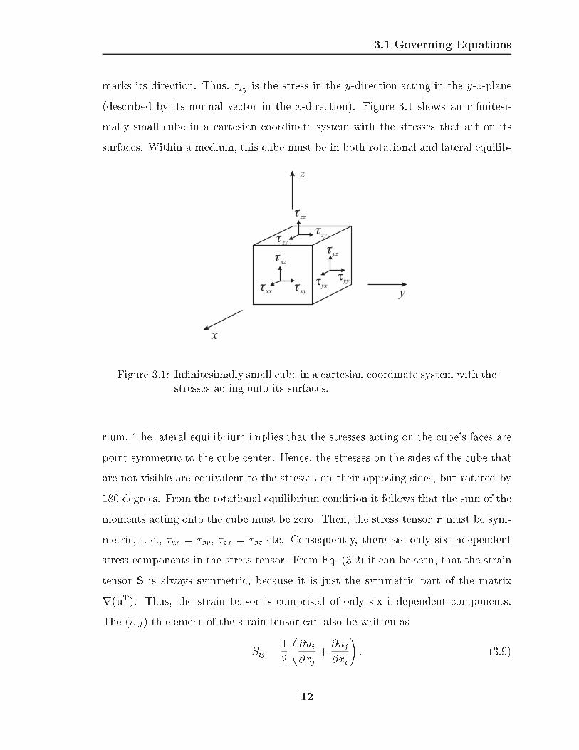
marks its direction. Thus, �xy is the stress in the y-direction acting in the y-z-plane
(described by its normal vector in the x-direction). Figure 3.1 shows an in�nitesi-
mally small cube in a cartesian coordinate system with the stresses that act on its
surfaces. Within a medium, this cube must be in both rotational and lateral equilib-
x
y
z
�xx �xy
�xz
�yy�yx
�yz
�zz
�zy�zx
Figure 3.1: In�nitesimally small cube in a cartesian coordinate system with thestresses acting onto its surfaces.
rium. The lateral equilibrium implies that the stresses acting on the cube's faces are
point-symmetric to the cube center. Hence, the stresses on the sides of the cube that
are not visible are equivalent to the stresses on their opposing sides, but rotated by
180 degrees. From the rotational equilibrium condition it follows that the sum of the
moments acting onto the cube must be zero. Then, the stress tensor � must be sym-
metric, i. e., �yx = �xy, �zx = �xz etc. Consequently, there are only six independent
stress components in the stress tensor. From Eq. (3.2) it can be seen, that the strain
tensor S is always symmetric, because it is just the symmetric part of the matrix
r(uT). Thus, the strain tensor is comprised of only six independent components.
The (i; j)-th element of the strain tensor can also be written as
Sij =1
2
@ui@xj
+@uj@xi
!: (3.9)
12

3.2 Elastic Waves in Isotropic Media
3.2 Elastic Waves in Isotropic Media
3.2.1 The Wave Equation in Isotropic Media
In isotropic media, the entries of the sti�ness matrix c can be completely described
in terms of two independent constants. These constants are called Lame's constants
and are denoted by � and �. Using Lame's constants, the constitutive relation for
the six unknown stress components reduces to
�xx = (�+ 2�)Sxx + �Syy + �Szz (3.10)
�yy = �Sxx + (�+ 2�)Syy + �Szz (3.11)
�zz = �Sxx + �Syy + (�+ 2�)Szz (3.12)
�yz = 2�Syz (3.13)
�xz = 2�Sxz (3.14)
�xy = 2�Sxy: (3.15)
Using equation (3.2), the strain can be expressed in terms of the displacement:
�xx = (�+ 2�)@ux@x
+ �@uy@y
+ �@uz@z
(3.16)
�yy = �@ux@x
+ (�+ 2�)@uy@y
+ �@uz@z
(3.17)
�zz = �@ux@x
+ �@uy@y
+ (�+ 2�)@uz@z
(3.18)
�yz = �(@uy@z
+@uz@y
) (3.19)
�xz = �(@ux@z
+@uz@x
) (3.20)
13

3.2 Elastic Waves in Isotropic Media
�xy = �(@ux@y
+@uy@x
): (3.21)
Finally, combining Eq. (3.1) with Eqs. (3.16){(3.21) and assuming that no body
forces are present (F = 0), the elastic wave equation for the three displacement
components in x, y and z is obtained:
�r2ux + (�+ �)(@2ux@x2
+@2uy@x@y
+@2uz@x@z
) = �@2ux@t2
(3.22)
�r2uy + (�+ �)(@2uy@y2
+@2uz@y@z
+@2ux@y@x
) = �@2uy@t2
(3.23)
�r2uz + (�+ �)(@2uz@z2
+@2ux@z@x
+@2uy@z@y
) = �@2uz@t2
; (3.24)
where r2 is the Laplace operator: r2 = @2
@x2+ @2
@y2+ @2
@z2.
Regrouping Eqs. (3.22){(3.24) and using vector notation, the vector wave equa-
tion is obtained:
(�+ 2�)r � r � u� �r�r� u = �@2u
@t2: (3.25)
3.2.2 Propagating Waves
Generally, the elastic wave equation gives rise to two di�erent kinds of waves prop-
agating in an elastic solid: a longitudinal wave referred to as pressure wave and a
transverse wave called shear wave. Both waves are propagating independently of each
other with di�erent phase velocities. The wave number for the pressure wave can be
written as
k2P =!2�
(�+ 2�)(3.26)
with the corresponding phase velocity cP =q
�+2��
. The wave number for the shear
wave, similarly, can be expressed as
k2S =!2�
�(3.27)
14

3.2 Elastic Waves in Isotropic Media
with its phase velocity cS =q
��. Since � and � are both always positive, the phase
velocity of the longitudinal wave is always larger than the phase velocity of the trans-
verse wave.
When a boundary or discontinuity is introduced, the existence of both longitu-
dinal and transverse waves in an elastic medium gives rise to additional waves. The
most important of these is the Rayleigh surface wave2 and appears at a free surface
boundary.
At a free surface (i. e., at the interface between an elastic medium and vacuum),
the normal stress components vanish due to the continuity of the normal stress at an
interface. Both the longitudinal and the transverse wave traveling along a free surface
cannot ful�ll this boundary condition by themselves. However, a combination of the
two can, giving rise to the Rayleigh surface wave.
Rayleigh surface waves have characteristic properties that distinguish them from
longitudinal and transverse waves. Rayleigh surface waves travel along the surface
and decay exponentially into the medium. The reach of the surface wave into the
medium is dependent on frequency. The higher the frequency, the faster the surface
wave decays into the medium. Due to their origin, surface waves are neither purely
longitudinal nor purely transverse. The particles that are subjected to a surface
wave instead undergo an elliptic motion, due to the superposition of longitudinal and
transverse �eld components. A surface wave travels with a phase velocity slightly
smaller than the phase velocity of the transverse wave and, thus, is slower than
both the longitudinal and the transverse wave. The wave speed of the surface wave
cannot be determined explicitly, but is de�ned by a transcendental equation. Since
the surface wave is traveling along a plane (i. e., the surface of a medium), it has a
somewhat two-dimensional character. While longitudinal and transverse waves due
to a point source in a three-dimensional medium decay proportionally to the inverse
of the distance from the source(/ r�1), a surface wave decays with the inverse of
2After Lord Rayleigh, who discovered the existence of elastic surface waves in the late nineteenthcentury.
15

3.2 Elastic Waves in Isotropic Media
the square root of the distance (/ r�1=2). Thus, its energy is in some way con�ned
to the surface. Moreover, if a two-dimensional case is considered (e. g., an in�nite
line source in a three dimensional medium), the surface wave has a one-dimensional
character and does not decay at all with distance from the source. This property of
con�nement of energy to a surface is most successfully used in Surface Acoustic Wave
(SAW) devices.
Figure 3.2 shows the elastic waves in the ground due to a point-like excitation
on the ground's surface.3 The particle displacement on a cross section through the
ground is plotted in a pseudo color plot. A logarithmic scale is used, where dark red
corresponds to the largest magnitude (0 dB) and blue to the smallest (�70 dB). Thetop edge of the plot coincides with the free surface. The excitation is a di�erentiated
Gaussian pulse. The pressure wave and the shear wave are visible. Both describe
spherical wave fronts. The Rayleigh surface wave propagates along the surface. At
the surface, plane waves arise. One is a lateral wave and is due to the passage of
the pressure wave along the surface , inducing a plane shear wave. The other one is
a leaky surface wave. The origin of this wave will be discussed in detail in a later
chapter.
3The wave �elds are computed with the numerical model which is described in the subsequentchapter.
16

3.2 Elastic Waves in Isotropic Media
x
z
Leaky Surface Wave Rayleigh Wave
Shear Wave
Pressure Wave
Lateral Wave
Figure 3.2: Elastic waves due to a point source on a free surface.
17

CHAPTER 4
Numerical Model
During the development of the elastic/electromagntic sensor, experiments have been
performed with mines buried in a large sand tank [12]. In these experiments, elas-
tic waves are excited by an electrodynamic transducer placed on the surface of the
ground. The waves propagate in the ground and along its surface and interact with
the buried land mines. To investigate the interactions of the elastic waves with the
buried mines, a three-dimensional �nite-di�erence model has been developed. In this
chapter, the �nite-di�erence model and its implementation are described.
4.1 The Finite-Di�erence Scheme
4.1.1 Problem Statement
Fig. 4.1 outlines the problem geometry. A transducer (labeled Source) is placed on
the surface of the ground. The transducer launches elastic waves, which interact with
an Object that is buried in the ground at some distance from the transducer. When
adapting this problem to a numerical model, assumptions must be made to simplify
the model and to make its implementation feasible. For the numerical model, the
ground is assumed to be a semi-in�nite half-space, bounded only by the surface at
z = 0. Thus, the tank with its walls as used in the experiments is not modeled and its
e�ects are neglected. The ground is approximated to be linear, isotropic, and lossless.
Within a numerical model, the elastic wave �elds are computed at a number of
18

4.1 The Finite-Di�erence Scheme
z
x
y
x
Air
Ground
Source
Object
Figure 4.1: Problem geometry; top: isometric view, bottom: cross sectionalview.
19

4.1 The Finite-Di�erence Scheme
discrete points in space. For the �nite-di�erence modeling scheme, a discrete grid of
regular cubic shape is introduced. Within the numerical model, the in�nite half-space
must be truncated and appropriate boundary conditions must be implemented to
avoid arti�cial re ections at the outer grid faces. Figure 4.2 shows a schematic drawing
of the three-dimensional �nite-di�erence model. The solution space is bounded on
top by a free-surface boundary and on all other sides by a Perfectly-Matched Layer
(PML) absorbing boundary. The source is located on the free surface.
4.1.2 Governing Equations
As described in Chapter 3, elastic wave propagation in a linear medium is governed by
three fundamental partial di�erential equations: the equation of motion, the strain-
displacement relation, and the elastic constitutive relation. By eliminating the strain,
a system of partial di�erential equations is obtained that describes the wave �elds in
terms of solely the displacement and the stress:
�@2ux@t2
=@�xx@x
+@�xy@y
+@�xz@z
(4.1)
�@2uy@t2
=@�xy@x
+@�yy@y
+@�yz@z
(4.2)
�@2uz@t2
=@�xz@x
+@�yz@y
+@�zz@z
(4.3)
�xx = (�+ 2�)@ux@x
+ �@uy@y
+ �@uz@z
(4.4)
�yy = �@ux@x
+ (�+ 2�)@uy@y
+ �@uz@z
(4.5)
�zz = �@ux@x
+ �@uy@y
+ (�+ 2�)@uz@z
(4.6)
�yz = �(@uy@z
+@uz@y
) (4.7)
20

4.1 The Finite-Di�erence Scheme
Object
PML
SourceFree Surface
Figure 4.2: Three-dimensional �nite-di�erence model.
21

4.1 The Finite-Di�erence Scheme
�xz = �(@ux@z
+@uz@x
) (4.8)
�xy = �(@ux@y
+@uy@x
): (4.9)
Two approaches can be chosen to adapt the governing equations to the �nite-
di�erence scheme. First, the wave equations for the displacement �eld components,
as described in Eqs. (3.22){(3.24), can be discretized [19]. This results in only three
equations with three unknowns. However, due to the second order character of the
wave equations, the �nite-di�erence equations are complicated. A di�erent approach
is to discretize Eqs. (4.1){(4.9) [26, 27]. The resulting system of equations includes
nine equations with nine unknowns. The equations contain only �rst-order deriva-
tives, if the particle velocity is introduced for the particle displacement. These equa-
tions are simple and, hence, can be implemented in a straightforward way. With the
�rst-order approach, the implementation of boundary conditions, for example, is con-
siderably easier than with the second-order approach. Because of its simplicity, the
�rst-order approach is now the most common approach for �nite-di�erence modeling
in elastodynamics.
To eliminate the second-order time-derivatives from Eqs. (4.1){(4.9), the particle
velocity is introduced for the displacement. The particle velocity is the time derivative
of the displacement:
v =@u
@t: (4.10)
Taking the time derivative of Eq. (4.4) { (4.9) and replacing @ux@t
with vx etc., one
obtains a system of equations with only derivatives of �rst order:
�@vx@t
=@�xx@x
+@�xy@y
+@�xz@z
(4.11)
�@vy@t
=@�xy@x
+@�yy@y
+@�yz@z
(4.12)
�@vz@t
=@�xz@x
+@�xz@y
+@�zz@z
(4.13)
22
4.1 The Finite-Di�erence Scheme
@�xx@t
= (�+ 2�)@vx@x
+ �@vy@y
+ �@vz@z
(4.14)
@�yy@t
= �@vx@x
+ (�+ 2�)@vy@y
+ �@vz@z
(4.15)
@�zz@t
= �@vx@x
+ �@vy@y
+ (�+ 2�)@vz@z
(4.16)
@�yz@t
= �(@vy@z
+@vz@y
) (4.17)
@�xz@t
= �(@vx@z
+@vz@x
) (4.18)
@�xy@t
= �(@vx@y
+@vy@x
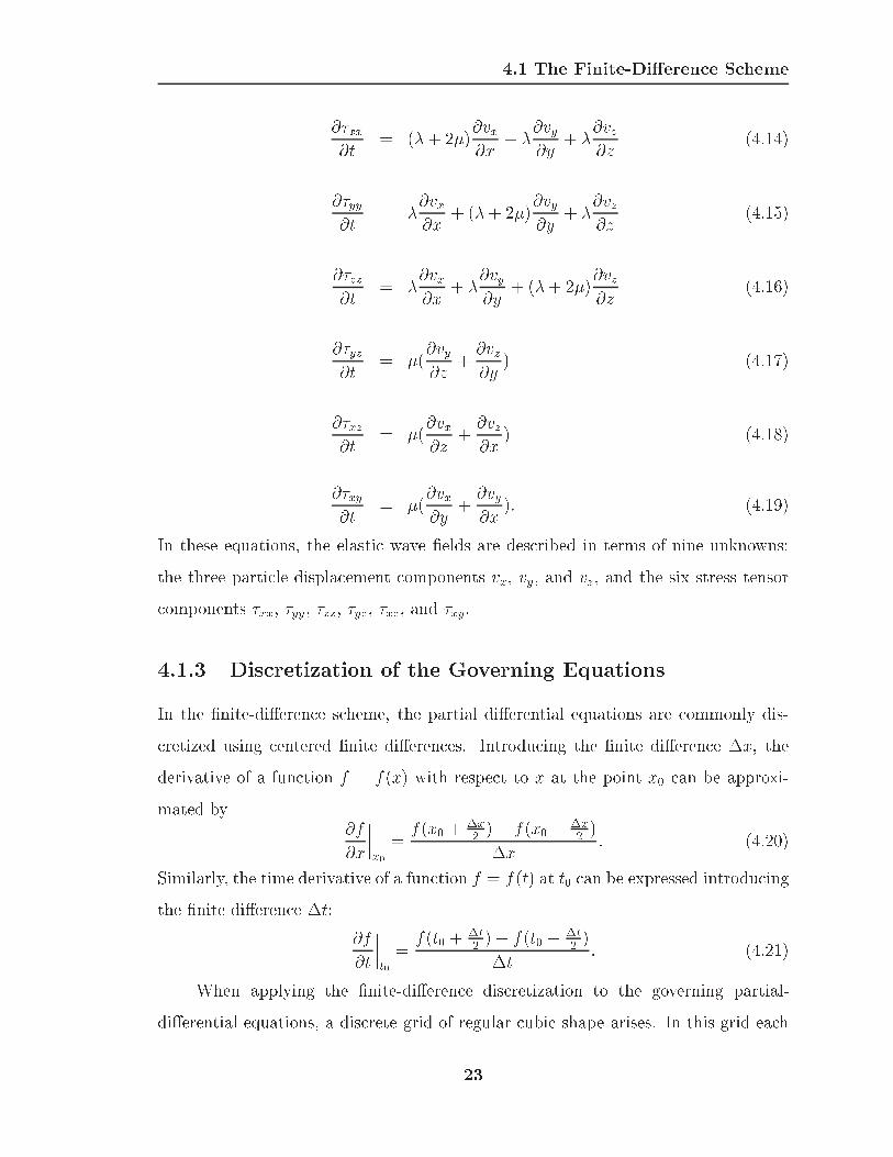
): (4.19)
In these equations, the elastic wave �elds are described in terms of nine unknowns:
the three particle displacement components vx, vy, and vz, and the six stress tensor
components �xx, �yy, �zz, �yz, �xz, and �xy.
4.1.3 Discretization of the Governing Equations
In the �nite-di�erence scheme, the partial di�erential equations are commonly dis-
cretized using centered �nite di�erences. Introducing the �nite di�erence �x, the
derivative of a function f = f(x) with respect to x at the point x0 can be approxi-
mated by@f
@x
����x0
=f(x0 +
�x2)� f(x0 � �x
2)
�x: (4.20)
Similarly, the time derivative of a function f = f(t) at t0 can be expressed introducing
the �nite di�erence �t:
@f
@t
����t0
=f(t0 +
�t2)� f(t0 � �t
2)
�t: (4.21)
When applying the �nite-di�erence discretization to the governing partial-
di�erential equations, a discrete grid of regular cubic shape arises. In this grid each
23

4.1 The Finite-Di�erence Scheme
�eld component is surrounded by the �eld components it is dependent on [27]. One
important characteristic of the �nite-di�erence grid is that the displacement and
stress components are not known at the same points in space and time. The resulting
�nite-di�erence expressions are centered around the �eld components to be deter-
mined. The structure of the �nite-di�erence grid is very similar to the one used for
electromagnetic �nite-di�erence modeling, where the so-called Yee-cell is introduced
[17].
The �nite-di�erence grid can be viewed as being composed of basis cells. Each
basis cell is characterized by its dimensions in x, y, and z, i. e., the �nite di�erences
�x, �y, and �z, and the position of the cell center in the grid. By introducing the
indices i, j, and k for the position of the cell in x, y, and z, respectively, the position
of the center is labeled and in that way uniquely identi�ed within the grid. Fig. 4.3
shows the (i; j; k)-th basis cell of the three-dimensional �nite-di�erence grid with its
elastic �eld components. The numerical (discrete) velocity components are indicated
by V and the numerical stress tensor components by T . In Fig. 4.4, a larger portion
of the �nite-di�erence grid is depicted.
The position of the cell center in real space is given by x = i ��x, y = j ��y,and z = k � �z. However, no �eld component is located at the cell center. The
positions of the �eld components of the (i; j; k)-th cell in real space are given in
Table 4.1. To uniquely identify the �eld components in the �nite-di�erence grid, only
the �eld components on the corners of the shaded region in Fig. 4.3 are assigned to
the (i; j; k)-th basis cell.
The discrete time is labeled with the index l. Due to the centered �nite-di�erence
formulation, half indices must be introduced for the velocity equations. Assuming the
incremental time of the �nite-di�erence algorithm to be �t, the values for the stress
tensor components are arbitrarily set to be known at the full time step, t = l ��t, andthe particle velocity components are calculated at the half time step, t = (l+0:5) ��t.
Introducing �nite di�erences in space and time, the partial-di�erential equa-
tions are discretized and discrete di�erence equations approximating the di�erential
24

4.1 The Finite-Di�erence Scheme
Vx
Vy
Vz
T , T , Txx yy zz
Tyz
Txz
Txy
�x
�z
�y
x i[ ]
y j[ ]
z k[ ]
Figure 4.3: Three-dimensional �nite-di�erence basis cell.
equations are obtained. For example, applying the discretization to Eq. (4.11) yields
�V l+0:5x ji;j;k � V l�0:5
x ji;j;k�t
=T lxxji;j;k � T l
xxji�1;j;k�x
+
+T lxyji;j;k � T l
xxji;j�1;k�y
+T lxzji;j;k � T l
xzji;j;k�1�z
: (4.22)
Here, the capital letters mark the numerical values of the �eld components at their
discrete locations in space and time. The notation is such that V l+0:5x ji;j;k, for example,
stands for the numerical value of the particle velocity vx at the (i; j; k)-th cell at time
t = (l + 0:5)�t.
By rearranging the di�erence equation, an equation for Vx at the incremented
time t = (l+0:5)�t can be obtained entirely in terms of �eld components at previous
times. Thus, if the �eld values at and prior to t = l�t are known, Vx at the incre-
mented time t = (l+0:5)�t can be computed. In the same way, each �eld component
can be expressed in terms of the previous �eld values. The resulting equations are
25

4.1 The Finite-Di�erence Scheme
Figure 4.4: A portion of the three-dimensional �nite-di�erence grid.
26

4.1 The Finite-Di�erence Scheme
Table 4.1: Positions of the �eld components of the (i; j; k)-th cell in the �nite-di�erence grid.
x y z
Vx i�x (j � 0:5)�y (k � 0:5)�z
Vy (i + 0:5)�x j�y (k � 0:5)�z
Vz (i + 0:5)�x (j � 0:5)�y k�z
Txx (i + 0:5)�x (j � 0:5)�y (k � 0:5)�z
Tyy (i + 0:5)�x (j � 0:5)�y (k � 0:5)�z
Tzz (i + 0:5)�x (j � 0:5)�y (k � 0:5)�z
Tyz (i + 0:5)�x j�y k�z
Txz i�x (j � 0:5)�y k�z
Txy i�x j�y (k � 0:5)�z
commonly called the �nite-di�erence update equations. The complete set of update
equations for the nine �eld components of the (i; j; k)-th grid cell is given by
V l+0:5x ji;j;k = V l�0:5
x ji;j;k + �t
��"T lxxji;j;k � T l
xxji�1;j;k�x
+ (4.23)
+T lxyji;j;k � T l
xyji;j�1;k�y
+T lxzji;j;k � T l
xzji;j;k�1�z
#
V l+0:5y ji;j;k = V l�0:5
y ji;j;k + �t
��"T lxyji+1;j;k � T l
xyji;j;k�x
+ (4.24)
+T lyyji;j+1;k � T l
yyji;j;k�y
+T lyzji;j;k � T l
yzji;j;k�1�z
#
V l+0:5z ji;j;k = V l�0:5
z ji;j;k + �t
��"T lxzji+1;j;k � T l
xzji;j;k�x
+ (4.25)
27

4.1 The Finite-Di�erence Scheme
+T lyzji;j;k � T l
yzji;j�1;k�y
+T lzzji;j;k+1 � T l
zzji;j;k�z
#
T l+1xx ji;j;k = T l
xxji;j;k +�t �"(�+ 2�)
V l+0:5x ji+1;j;k � V l+0:5
x ji;j;k�x
+ (4.26)
+ �V l+0:5y ji;j;k � V l+0:5
y ji;j�1;k�y
+ �V l+0:5z ji;j;k � V l+0:5
z ji;j;k�1�z
#
T l+1yy ji;j;k = T l
yyji;j;k +�t �"�V l+0:5x ji+1;j;k � V l+0:5
x ji;j;k�x
+ (4.27)
+ (�+ 2�)V l+0:5y ji;j;k � V l+0:5
y ji;j�1;k�y
+ �V l+0:5z ji;j;k � V l+0:5
z ji;j;k�1�z
#
T l+1zz ji;j;k = T l
zzji;j;k +�t �"�V l+0:5x ji+1;j;k � V l+0:5
x ji;j;k�x
+ (4.28)
+ �V l+0:5y ji;j;k � V l+0:5
y ji;j�1;k�y
+ (�+ 2�)V l+0:5z ji;j;k � V l+0:5
z ji;j;k�1�z
#
T l+1yz ji;j;k = T l
yzji;j;k +�t � �"V l+0:5z ji;j+1;k � V l+0:5
z ji;j;k�y
+ (4.29)
+V l+0:5y ji;j;k+1 � V l+0:5
y ji;j;k�z
#
T l+1xz ji;j;k = T l
xzji;j;k +�t � �"V l+0:5z ji;j;k � V l+0:5
z ji�1;j;k�x
+ (4.30)
+V l+0:5x ji;j;k+1 � V l+0:5
x ji;j;k�z
#
T l+1xy ji;j;k = T l
xyji;j;k +�t � �"V l+0:5y ji;j;k � V l+0:5
y ji�1;j;k�x
+ (4.31)
28

4.1 The Finite-Di�erence Scheme
+V l+0:5x ji;j+1;k � V l+0:5
x ji;j;k�y
#:
Note that the velocity components are computed at the half time steps, whereas the
stress components are determined at the full time steps.
The �nite-di�erence scheme, then, works as follows. Initially, i. e., at l = 0, the
values of all �eld components are set to zero. At one point or in an entire region
(i. e., in the source region) an elastic �eld is excited. The velocity components are
updated throughout the grid for l = 0:5, and using the velocities at l = 0:5 the stress
components are calculated for l = 1. Then the velocities are computed for l = 1:5 from
the stresses at l = 1 and so on. Following this procedure, sequentially the velocity and
stress �elds can be calculated up to any desired time. Due to the gradual progressing
in time by \hopping" from the stresses to the velocities, the algorithm is commonly
referred to as leapfrog scheme [17].
General constraints on the size of the space increments �x, �y, and �z and
the time increment �t arise. To compute the elastic wave �elds with a reasonable
accuracy, the space step must not exceed one tenth of the minimum wave length
excited within the model [17]:
�x;�y;�z < �min=10: (4.32)
By obeying this condition, arti�cial numerical dispersion e�ects are minimized. The
time increment is linked to the space increment by the general condition for stability,
the Courant condition:
cmax�t
s1
�x2+
1
�y2+
1
�z2� 1; (4.33)
where cmax is the maximum wave speed occurring in the numerical model. If �x =
�y = �z, this reduces to
cmax�t
�x� 1p
3: (4.34)
In plain words, the Courant condition states that the physical wave speed of any wave
excited in the model must not exceed the speed information can travel with in the
numerical grid.
29
4.2 Boundaries
4.2 Boundaries
When implementing the �nite-di�erence scheme, boundary conditions have to be
treated in a special manner. Three di�erent kinds of boundaries arise: points or re-
gions where the �elds are excited (i. e., the source), internal boundaries (i. e., bound-
aries within the medium caused by a change in material properties), and external
boundaries (i. e., the outer grid faces).
4.2.1 Source
Elastic wave �elds can be excited at any point in space. For most of the results
that are presented in this thesis, a source is used that emulates the transducer used
in the experiments. For this, the vertical particle velocity component, vz, is excited
on the surface throughout a region of approximately the same shape and size as the
transducer foot. A di�erentiated Gaussian pulse is used as excitation, which closely
resembles the transducer foot motion. For some results, instead of modeling the
transducer, a plane wave is injected. This requires a special formulation, which is
described in Sec. 4.3.
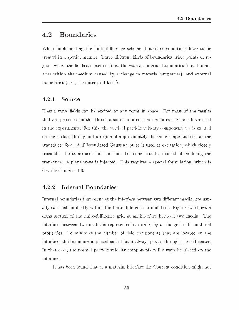
4.2.2 Internal Boundaries
Internal boundaries that occur at the interface between two di�erent media, are usu-
ally satis�ed implicitly within the �nite-di�erence formulation. Figure 4.5 shows a
cross section of the �nite-di�erence grid at an interface between two media. The
interface between two media is represented naturally by a change in the material
properties. To minimize the number of �eld components that are located on the
interface, the boundary is placed such that it always passes through the cell center.
In that case, the normal particle velocity components will always be placed on the
interface.
It has been found that at a material interface the Courant condition might not
30

4.2 Boundaries
z
x
i�1 i i+1
k+1
k�1
k
Medium 2Medium 1
Vx i j k| , ,
Txz i j k| , , -1
Figure 4.5: Schematic drawing of the �nite-di�erence grid at the interface be-tween two media. The normal particle velocity components arealways located on the interface.
be a suÆcient condition for stability of the �nite-di�erence algorithm. To ensure that
the Courant condition is a suÆcient stability condition, the material properties must
be averaged for all �eld components located on the boundary. A discussion of the
stability of the �nite-di�erence algorithm at a material interface and a derivation of
the averaging procedure is given in Chapter 5.
At an interface between two media, say Medium 1 and Medium 2, the averaged
31

4.2 Boundaries
material density and the averaged shear sti�ness are
�avg =�Medium 1 + �Medium 2
2(4.35)
�avg =2
1�Medium 1
+ 1�Medium 2
: (4.36)
The longitudinal sti�ness does not have to be averaged, because, due to the placement
of the interface, the longitudinal stresses will never lie on the boundary. Note that
the inverse of the shear sti�ness is averaged.
In the discrete �nite-di�erence grid, the material density and the shear sti�ness
are known at the locations of the particle velocity components and the shear stresses,
respectively. For example, in the cross section in Fig. 4.5, Vxji;j;k lies on the interface,
and at its location the material density is averaged:
�avgji;j;k = (�ji�1;j;k + �ji;j;k) =2: (4.37)
At the location of the shear stress Txzji;j;k�1, the averaged shear sti�ness is
�avgji;j;k�1 = 2
1
�ji;j;k�1 +1
�ji�1;j;k�1
!�1
: (4.38)
For the shear stress on the corner of the interface (which corresponds to an edge if
the grid is expanded to its three dimensions), the shear sti�ness must be averaged
between all four adjacent cells:
�avgji;j;k = 4
1
�ji;j;k +1
�ji�1;j;k +1
�ji;j;k+1 +1
�ji�1;j;k+1
!�1
: (4.39)
The averaging is performed in an analogous manner for all �eld components on the
interface.
4.2.3 Free-Surface Boundary
Six external boundaries arise at the six outer grid faces of the numerical model.
Contrary to internal boundaries, external boundaries have to be treated explicitly to
satisfy the required boundary conditions.
32
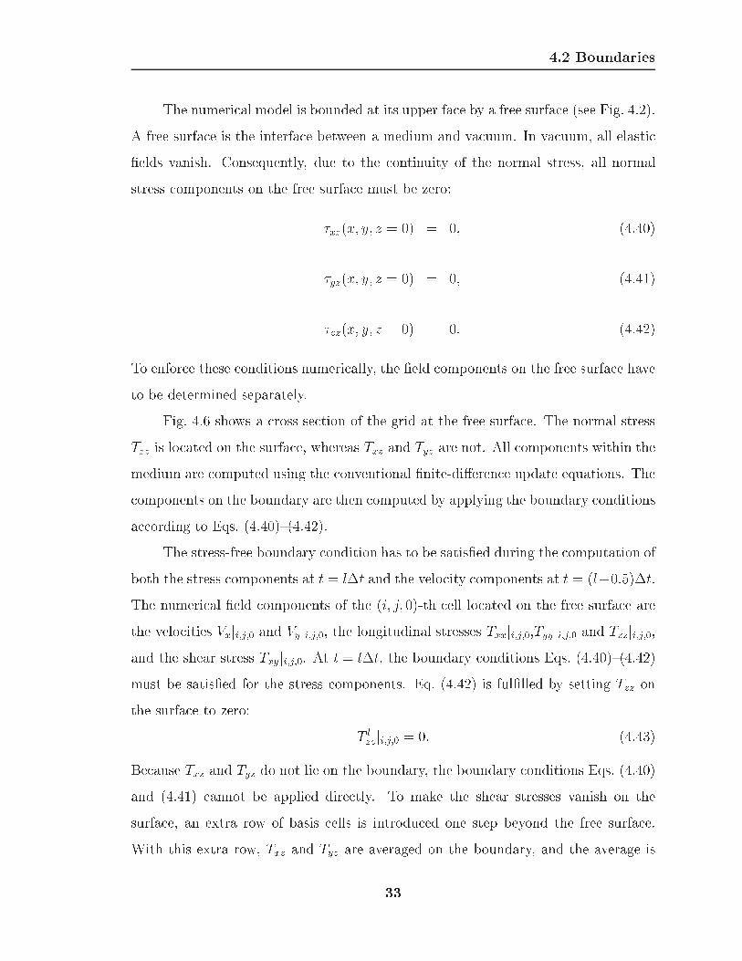
4.2 Boundaries
The numerical model is bounded at its upper face by a free surface (see Fig. 4.2).
A free surface is the interface between a medium and vacuum. In vacuum, all elastic
�elds vanish. Consequently, due to the continuity of the normal stress, all normal
stress components on the free surface must be zero:
�xz(x; y; z = 0) = 0; (4.40)
�yz(x; y; z = 0) = 0; (4.41)
�zz(x; y; z = 0) = 0: (4.42)
To enforce these conditions numerically, the �eld components on the free surface have
to be determined separately.
Fig. 4.6 shows a cross section of the grid at the free surface. The normal stress
Tzz is located on the surface, whereas Txz and Tyz are not. All components within the
medium are computed using the conventional �nite-di�erence update equations. The
components on the boundary are then computed by applying the boundary conditions
according to Eqs. (4.40){(4.42).
The stress-free boundary condition has to be satis�ed during the computation of
both the stress components at t = l�t and the velocity components at t = (l+0:5)�t.
The numerical �eld components of the (i; j; 0)-th cell located on the free surface are
the velocities Vxji;j;0 and Vyji;j;0, the longitudinal stresses Txxji;j;0,Tyyji;j;0 and Tzzji;j;0,and the shear stress Txyji;j;0. At t = l�t, the boundary conditions Eqs. (4.40){(4.42)
must be satis�ed for the stress components. Eq. (4.42) is ful�lled by setting Tzz on
the surface to zero:
T lzzji;j;0 = 0: (4.43)
Because Txz and Tyz do not lie on the boundary, the boundary conditions Eqs. (4.40)
and (4.41) cannot be applied directly. To make the shear stresses vanish on the
surface, an extra row of basis cells is introduced one step beyond the free surface.
With this extra row, Txz and Tyz are averaged on the boundary, and the average is
33

4.2 Boundaries
z
x
Free Surface
ii�1
k = 0
k = 1�
k = 1
Medium
Txz|i j, , 1�
Tzz|i j, ,0
Txz|i j, ,0
Vz|i j, , 1�
Figure 4.6: Finite di�erence grid and its �eld components at the free surface;cross section at y = (j � 0:5)�y. An extra row at k = �1 mustbe inserted to satisfy the stress-free boundary condition at the freesurface.
set to zero:
�T lxzji;j;�1 + T l
xzji;j;0�=2 = 0 (4.44)
�T lyzji;j;�1 + T l
yzji;j;0�=2 = 0: (4.45)
Because T lxzji;j;0 and T l
yzji;j;0 lie within the medium, they are determined together
with the �eld components in the medium using the normal update equations. Thus,
Eqs. (4.44) and (4.45) can be used to determine the shear stresses on the extra row
34

4.2 Boundaries
beyond the boundary:
T lxzji;j;�1 = �T l
xzji;j;0 (4.46)
T lyzji;j;�1 = �T l
yzji;j;0: (4.47)
Finally, knowing the velocity components on the free surface and on the extra row
from the previous time step, T lxxji;j;0, T l
yyji;j;0, and T lxyji;j;0 on the boundary are calcu-
lated using the normal update equations.
At t = (l + 0:5)�t, the velocity components are determined. Using the stress
components on the surface and on the inserted row, the velocity components, includ-
ing the ones on the surface, can be updated using the normal update equations. The
only velocity component that cannot be obtained in this manner is V l+0:5z ji;j;�1 on
the inserted row. Instead, V l+0:5z ji;j;�1 is obtained by setting T l+1
zz ji;j;0 to zero within
Eq. (4.28) according to (4.42). One obtains
0 = (�+ 2�)�t
�z(V l+0:5
z ji;j;0 � V l+0:5z ji;j;�1)
+ ��t
�x(V l+0:5
x ji+1;j;0 � V l+0:5x ji;j;0) (4.48)
+ ��t
�y(V l+0:5
y ji;j;0 � V l+0:5y ji;j�1;0): (4.49)
By rearranging, Vz on the extra row is determined:
V l+0:5z ji;j;�1 = V l+0:5
z ji;j;0 + �
�+ 2��
� �z
�x(V l+0:5
x ji+1;j;0 � V l+0:5x ji;j;0) +
+�z
�y(V l+0:5
y ji;j;0 � V l+0:5y ji;j�1;0)
!: (4.50)
Vzji;j;�1 is necessary to calculate the stress components on the surface at the next time
35

4.2 Boundaries
step. Following this scheme, the stress-free boundary condition is satis�ed across the
entire surface, and all �eld components on the surface are determined.
4.2.4 Perfectly-Matched Layer Absorbing Boundary
To model the in�nite extent of the half space, the waves that reach the outer grid
faces must be absorbed. The boundary condition that does this most accurately is
the Perfectly Matched Layer boundary condition. The particular formulation that is
used here has been developed by Chew and Liu [55].
The Perfectly Matched Layer (PML) boundary condition was �rst introduced by
Berenger [49] for the �nite-di�erence modeling of electromagnetic wave propagation,
then simpli�ed for example by Sacks [50] and Gedney [51] and adapted to the elastic
case by Chew and Liu [55]. A PML is a boundary layer consisting of a lossy material,
in which waves are propagating with exactly the same phase velocity and the exact
same wave impedance as waves in the solution space. Arbitrarily polarized waves
incident on the PML are perfectly transmitted and then attenuated within the PML.
In order to match the PML to the medium of the solution space, the �eld quantities
must be split, leading to a set of non-physical equations.
Chew and Liu interpret the PML as coordinate stretching in the frequency do-
main [55]. This can be understood as follows: given a plane wave propagating in a
lossless medium and described by the phasor ejkx0
, the stretching of coordinates rep-
resents a change of variables: x0 �! (1+ j�)x. The resulting plane wave is described
by e��xejkx and, thus, is attenuated in the x-direction due to the complex coordinate
stretching.
Introducing the nabla operator for stretched coordinates,
re =
2666664
1ex
@@x
1ey
@@y
1ez
@@z
3777775 ; (4.51)
where ex = 1+j�x, ey = 1+j�y and ez = 1+j�z represent the stretching factors, it can
36

4.2 Boundaries
be shown that a perfectly matched layer exists simultaneously for both pressure (P)
and vertical shear (SV) waves [55]. Considering an interface between Medium 1 and
Medium 2 at z = 0 normal to the z-direction, ez in (4.51) can be chosen di�erently in
Medium 1 and Medium 2 while still maintaining a perfectly matched interface between
the two media . For example, if Medium 1 is lossless in the z-direction (ez = 1) and
Medium 2 is lossy (ez = 1 + j�z), then Medium 1 will still be perfectly matched to
Medium 2, and a wave incident from Medium 1 onto Medium 2 will be transmitted
without any re ection. A theoretical derivation of the PML for elastodynamics is
given in [55].
The implementation of the PML for the discrete grid shall be explained here by
deriving the formulation for the velocity component vx from Eq. (4.11). Transform-
ing Eq. (4.11) into the frequency domain and introducing the coordinate-stretching
variables
ex = 1 + jx
!(4.52)
ey = 1 + jy
!(4.53)
ez = 1 + jz
!; (4.54)
one obtains
�j!�vx =1
1 + j x!
@�xx@x
+1
1 + j y!
@� xy@y
+1
1 + j z!
@� xz@z
; (4.55)
where the bar indicates quantities in the frequency domain. In order to dampen the
�elds independently in the x-, y- and z-direction, the �eld components must be split.
For each derivative in space, a new �eld component is introduced. Thus, three split
�eld components arise for Eq. (4.55), one for each term on the right hand side of the
equation:
�j!�vx;x =1
1 + j x!
@�xx@x
; (4.56)
37

4.2 Boundaries
�j!�vx;y =1
1 + j y!
@� xy@y
; (4.57)
�j!�vx;z =1
1 + j z!
@�xz@z
; and (4.58)
vx = vx;x + vx;y + vx;z: (4.59)
Rearranging Eqs. (4.56){(4.58) and transforming them back into the time do-
main, expressions for the split �elds in the time domain are obtained:
(�@
@t+ �x)vx;x =
@�xx@x
; (4.60)
(�@
@t+ �y)vx;y =
@�xy@y
; (4.61)
(�@
@t+ �z)vx;z =
@�xz@z
(4.62)
vx = vx;x + vx;y + vx;z (4.63)
The above set of equations can be discretized by introducing �nite di�erences. Note
that, when Eqs. (4.60){(4.62) are discretized, formally the velocities must be known
at the previous full and half time step. This is due to the fact that the velocities on
the left hand side appear once in their time-di�erentiated form and once in a non-
di�erentiated form. For example, in order to calculate V l+0:5x;x , both V l
x;x and V l�0:5x;x
must be known due to the fact that @vx;x@t
and vx;x appear in the governing equation
(see Eq. (4.60)). However, V lx;x can be approximated by V l
x;x = (V l+0:5x;x + V l�0:5
x;x )=2.
In that way, V lx;x is eliminated and only V l+0:5
x;x and V l�0:5x;x remain.
Altogether, 21 split �eld components arise from the original set of governing
equations. A set of 21 equations is derived, which, together with the nine combining
equations, form a complete set for the 21 split �eld components and the nine original
�eld components. The �nite-di�erence update equations for the split �eld formulation
can be found in Appendix A.
38
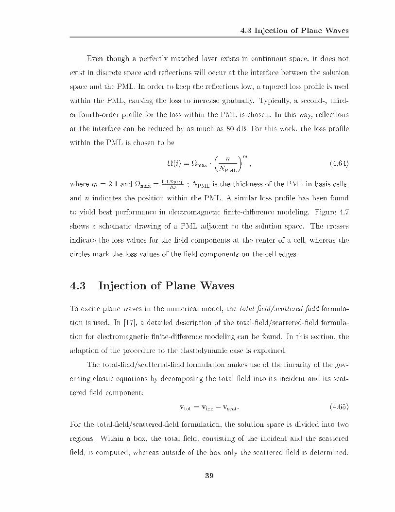
4.3 Injection of Plane Waves
Even though a perfectly matched layer exists in continuous space, it does not
exist in discrete space and re ections will occur at the interface between the solution
space and the PML. In order to keep the re ections low, a tapered loss pro�le is used
within the PML, causing the loss to increase gradually. Typically, a second-, third-
or fourth-order pro�le for the loss within the PML is chosen. In this way, re ections
at the interface can be reduced by as much as 80 dB. For this work, the loss pro�le
within the PML is chosen to be
(i) = max ��
n
NPML
�m; (4.64)
where m = 2:1 and max =0:1NPML
�t; NPML is the thickness of the PML in basis cells,
and n indicates the position within the PML. A similar loss pro�le has been found
to yield best performance in electromagnetic �nite-di�erence modeling. Figure 4.7
shows a schematic drawing of a PML adjacent to the solution space. The crosses
indicate the loss values for the �eld components at the center of a cell, whereas the
circles mark the loss values of the �eld components on the cell edges.
4.3 Injection of Plane Waves
To excite plane waves in the numerical model, the total-�eld/scattered-�eld formula-
tion is used. In [17], a detailed description of the total-�eld/scattered-�eld formula-
tion for electromagnetic �nite-di�erence modeling can be found. In this section, the
adaption of the procedure to the elastodynamic case is explained.
The total-�eld/scattered-�eld formulation makes use of the linearity of the gov-
erning elastic equations by decomposing the total �eld into its incident and its scat-
tered �eld component:
vtot = vinc + vscat: (4.65)
For the total-�eld/scattered-�eld formulation, the solution space is divided into two
regions. Within a box, the total �eld, consisting of the incident and the scattered
�eld, is computed, whereas outside of the box only the scattered �eld is determined.
39

4.3 Injection of Plane Waves
N xPML �
PML MediumNormal Medium
Lo
ssP
rofi
le,
�
0
�max
Figure 4.7: Schematic drawing of a PML layer in the x-direction: loss pro�leaccording to Eq. (4.64). The crosses and circles indicate the lossvalues of the �eld components at the center and at the edges of acell, respectively.
Fig. 4.8 illustrates schematically the division of the solution space into the two
regions, the inner Total-Field Region and the outer Scattered-Field Region. The struc-
ture that scatters the incident waves must necessarily be completely embedded in the
total-�eld region. Within the total-�eld region, the �nite-di�erence algorithm oper-
ates on the total-�eld components. In the outer region, no incident wave is present
and the algorithm operates only on the scattered �eld. The scattered-�eld region is
terminated by the boundary conditions at the outer grid faces, i. e., either by the
free-surface boundary condition or the PML absorbing boundary condition.
An arti�cial, non-physical interface will arise between the total-�eld region and
the scattered-�eld region. To provide the transition from the total-�eld region to the
40

4.3 Injection of Plane Waves
Scattered-Field Region
Total-Field Region
PML
Figure 4.8: Division of the solution space into a Total-Field Region and aScattered-Field Region. The scattering objects must be completelyembedded in the total-�eld region.
scattered-�eld region, all �eld components adjacent to the interface must be adjusted.
This is possible, if the incident �eld is known at all points in space and for all times. In
that case, the scattered �eld can be computed from the total �eld for the components
on the interface and vice versa.
4.3.1 Procedure
In each the total-�eld region and the scattered-�eld region, the conventional �nite-
di�erence update equations are applied to compute the �eld values. At the interface
between the two regions, the �eld components are adjusted. In general, a correction
term must be added to all �eld components that are dependent on �eld components
lying across the boundary.
Fig. 4.9 shows the �eld components at the interface on a cross section repre-
senting the x-z-plane and cutting through the in-plane velocity components Vx and
41

4.3 Injection of Plane Waves
and Vz. The �eld components at the interface are indicated in black. The interface
Vx
Vy
Vz
T , T , Txx yy zz
Tyz
Txz
Txy
Scattered Field
Total FieldVx i j l| , , Txx i j l| , ,
x
z
Figure 4.9: Both the �eld components just outside and just inside the total-�eldbox must be corrected with the known incident �elds.
is placed such that the longitudinal stresses will always lie on the edges and corners
of the bounding box for the inner total-�eld region.
The adjustment procedure is illustrated for Vxji;j;k and T l+1xx ji;j;k at the interface
to the left. Vxji;j;k lies in the scattered-�eld region just outside of the total-�eld region.To update the velocity components throughout the scattered-�eld region, the normal
�nite-di�erence equations are applied. The update equation for Vxji;j;k at the interfacethen becomes:
V l+0:5x;scat ji;j;k = V l�0:5
x;scat ji;j;k +�t
��"T lxx;scatji;j;k � T l
xx;scatji�1;j;k�x
+ (4.66)
+T lxy;scatji;j;k � T l
xy;scatji;j�1;k�y
+T lxz;scatji;j;k � T l
xz;scatji;j;k�1�z
#:
In this equation, T lxx;scatji;j;k is unknown, because Txx at the (i; j; k)-th cell lies in the
42

4.3 Injection of Plane Waves
total �eld region. However, T lxx;scatji;j;k can be computed from the total-�eld value, if
the incident �eld value is known:
T lxx;scatji;j;k = T l
xx;totji;j;k � T lxx;incji;j;k: (4.67)
Inserting this into Eq. (4.66), one obtains an update equation for Vxji;j;k at the inter-face in which all �eld components are known:
V l+0:5x;scat ji;j;k = V l�0:5
x;scat ji;j;k +�t
��"T lxx;totji;j;k � T l
xx;scatji�1;j;k�x
+
+T lxy;scatji;j;k � T l
xy;scatji;j�1;k�y
+T lxz;scatji;j;k � T l
xz;scatji;j;k�1�z
#�
� �t
��x� T l
xx;incji;j;k: (4.68)
The �eld components at the interface just inside the total-�eld region are treated
in a similar way. By applying the conventional update equation, T l+1xx ji;j;k at the
interface is obtained:
T l+1xx;totji;j;k = T l
xx;totji;j;k +�t �"(�+ 2�)
V l+0:5x;tot ji+1;j;k � V l+0:5
x;tot ji;j;k�x
+ (4.69)
+ �V l+0:5y;tot ji;j;k � V l+0:5
y;tot ji;j�1;k�y
+ �V l+0:5z;tot ji;j;k � V l+0:5
z;tot ji;j;k�1�z
#:
In this equation, V l+0:5x;tot ji;j;k is unknown, because it is located in the scattered-�eld
region. Using the incident �eld, an update equation with only known �eld values is
derived:
T l+1xx;totji;j;k = T l
xx;totji;j;k +�t �"(�+ 2�)
V l+0:5x;tot ji+1;j;k � V l+0:5
x;scat ji;j;k�x
+
+ �V l+0:5y;tot ji;j;k � V l+0:5
y;tot ji;j�1;k�y
+ �V l+0:5z;tot ji;j;k � V l+0:5
z;tot ji;j;k�1�z
#�
� �t(�+ 2�)
�x� V l+0:5
x;inc ji;j;k: (4.70)
43

4.3 Injection of Plane Waves
Usually, to simplify the implementation, the �eld components at the interface are
�rst computed using the conventional update equations and are then adjusted after
each time step. In three dimensions, six interfaces between the inner total-�eld region
and the outer scattered-�eld region arise. By applying the normal update equations
to the terms at the interface, equations containing both scattered- and total-�eld
components arise. These are inconsistent and must be corrected by adding a term
containing the incident-�eld component (see Eqs. (4.68) and (4.70)). A complete
listing of the �eld components at each interface and their corresponding correction
terms can be found in Appendix B.
4.3.2 Incident Field
To adjust the �eld components on the interface between the total-�eld and the
scattered-�eld region, the incident �eld must be known at all points in space at
all times. Various schemes are possible to predict the incident �eld. To describe an
incident plane wave, a one-dimensional �nite-di�erence formulation can be employed.
With the 1-D �nite-di�erence algorithm, the plane wave is computed separately us-
ing the same space and time increment as in the 3-D grid. By mapping the 1-D �eld
onto the 3-D grid, a look-up table is created that contains the incident �eld values for
all points in space and time. Using this look-up table, the �eld components at the
interfaces between the total- and scattered-�eld region are adjusted. A plane pressure
wave as well as a plane shear wave can be, in this way, injected into the grid.
Employing the 1-D �nite-di�erence algorithm to compute the incident �eld has
the further advantage that the incident �eld as a function of time and space is de-
scribed as it appears in the three-dimensional grid. By using a numerical algorithm
rather than an analytical description, the numerical wave speed in the grid, which
will slightly di�er from its analytical value, is emulated. Thus, a more accurate
adjustment of the �eld components on the interface can be achieved.
44

4.4 Parallelization
4.4 Parallelization
The three-dimensional �nite-di�erence model has been implemented using FORTRAN
90. The computational and memory requirements of the numerical model are im-
mense, and the computations usually cannot be performed on a conventional per-
sonal computer. Therefore, the model is implemented in a fully parallel fashion using
the Message-Passing Interface (MPI), and computers with a parallel architecture that
contain multiple processors are used.
In the model, the elastic wave �elds are computed on a three-dimensional discrete
grid. When implemented on a parallel computer, this grid is divided into several
sub-grids, and each sub-grid is assigned to one processor of the parallel machine
[17]. Fig. 4.10 visualizes the distribution of the processors across the computational
grid. Here, the grid is divided into eight sub-grids, and each sub-grid is assigned
to one processor. The processors then compute the wave �elds on their sub-grids
independently from each other and share the data on the common interfaces after
each time step. The procedure is algorithmically simple, but its implementation is
rather tedious. To improve the computational eÆciency of the parallel program, some
important guide lines should be followed. Most importantly, the amount of data that
is passed between the processors after each time step must be minimized. For this,
the grid is divided into sub-grids whose dimensions in all directions are approximately
equal. In that way, the surface area of the sub-grids, i. e., the face area that each
sub-grid shares with its neighbors and thus the amount of shared data, is minimal.
The computations for this work have been performed on a Cray T3E parallel
supercomputer at the ERDC Massively Shared Resource Center of the DoD, located
in Vicksburg, Mississippi, and on a Beowulf computer cluster [60]. The Beowulf
cluster is located at the Georgia Institute of Technology and contains 50 Pentium III
processors and 6 GBytes of memory.
45
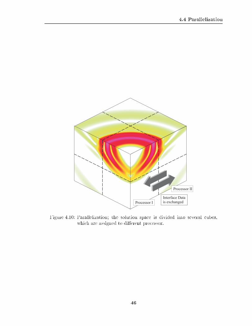
4.4 Parallelization
Processor I
Processor II
Interface Datais exchanged
Figure 4.10: Parallelization; the solution space is divided into several cubes,which are assigned to di�erent processor.
46

CHAPTER 5
Stability of the FDTD Algorithm at a
Material Interface
As described in Chapter 4, a �nite-di�erence model has been developed in two and
three dimensions that simulates the elastic wave propagation in the ground. During
the development of the �nite-di�erence model, instabilities in the algorithm occurred.
In the �nite-di�erence algorithm, internal boundaries, i. e., boundaries between
di�erent materials, are satis�ed implicitly. The �nite-di�erence algorithm is usually
stable, if the Courant condition is satis�ed. However, if media with greatly di�erent
material properties are considered, it turns out that the Courant condition is not
necessarily a suÆcient condition for stability, but a more restrictive condition arises.
One way to avoid the more restrictive stability condition is to average the material
parameters at the interface between two di�erent media.
In this chapter, the stability behavior of the �nite-di�erence scheme at a mate-
rial interface is analyzed. First, a longitudinal wave normally incident onto a material
interface is considered. The von-Neumann method and the matrix method are em-
ployed, and theoretical bounds for stability are established. It is shown that, if the
material parameters are averaged on the boundary, the Courant condition poses a
suÆcient condition for stability, and no further restrictions on the stability condi-
tion due to the presence of the material interface arise. Second, a numerical study
of stability in 1-D and 2-D is performed, and the theoretical bounds are validated.
47

5.1 Stability Analysis: Theory
Most importantly, it is shown that the FDTD algorithm in fact is stable whenever the
material properties are averaged on the boundary. Finally, the averaging procedure
is described.
The mathematical theorems and procedures presented in this chapter are well-
known. The stability analysis closely follows Richtmyer [61], Smith [62], and Mitchell
and GriÆths [63], who also provide a more thorough description of the mathematical
theory. A similar analysis of stability has been performed, for example, by Ilan
and Loewenthal, who investigated the stability of the second-order �nite-di�erence
formulation, based on the elastic wave equation, at a free-surface boundary [22].
5.1 Stability Analysis: Theory
The fundamental condition for stability of the �nite-di�erence algorithm, i. e., the
condition that relates the size of the time increment to the spacing of the discrete
nodes in the FDTD grid and that must be ful�lled for the �nite-di�erence algorithm
to be stable, is the Courant condition [64, 17]. The Courant condition states that the
physical wave speed of any wave excited in the model must not exceed the velocity
that information can travel with in the discrete grid. Mathematically, for a space
step of size �l, the Courant condition in an n-dimensional grid is
�t
�lcmax � 1p
n: (5.1)
Here, �t denotes the time step, and cmax is the maximum wave speed occurring in the
numerical model. Note that the Courant condition becomes more restrictive when
the number of dimensions is increased.
In this section, it is shown that the Courant condition by itself is not always a
suÆcient condition for stability, if a material interface is present. A theoretical bound
in terms of the material properties is derived beyond which the material parameters
must be averaged for the �nite-di�erence scheme to be stable. The bound is derived
using the von-Neumann method and the Matrix method for a 1-D longitudinal wave
48

5.1 Stability Analysis: Theory
incident onto a material interface.
5.1.1 1-D Longitudinal Wave Incident onto a Material Inter-
face
The stability behavior of a 1-D �nite-di�erence grid for a longitudinal wave normally
incident onto a material interface is to be investigated. The propagation direction
coincides with the x-direction, and the only non-zero velocity component is vx. Fig-
ure 5.1 shows a portion of the discrete �rst-order �nite-di�erence grid. The material
interface is located between Txx at i�0:5 and Vx at i. The �rst-order �nite-di�erence
system of equations can be combined to obtain a second-order formulation in terms
of solely the particle velocity. By combining the discrete �rst-order equations rather
than discretizing the second-order wave equation, the stability behavior of the �rst-
order �nite-di�erence formulation is preserved. In the second-order formulation, the
stress Txx is eliminated, but the Lam�e constants, which are associated with the stress
components, are still located half a step in between the velocity components. The
second-order �nite-di�erence update equation for the longitudinal particle velocity Vx
becomes
V k+1x jn = V k
x jn"2� �t2
�x2�jn�0:5 + 2�jn�0:5 + �jn+0:5 + 2�jn+0:5
�jn
#
+V kx jn+1
"�t2
�x2�jn+0:5 + 2�jn+0:5
�jn
#
+V kx jn�1
"�t2
�x2�jn�0:5 + 2�jn�0:5
�jn
#
�V k�1x jn; (5.2)
where n = 1 : : : N labels the nodes in the 1-D grid and k represents the discrete time
step. Again, note that the Lam�e constants are placed at the half steps in between
the velocity nodes.
49

5.1 Stability Analysis: Theory
x
Medium 1
ii�1 i+1
Vx
Txx
�x
Medium 2
�|i� �| + 2 |i i-0.5 -0.5
Figure 5.1: 1-D �nite-di�erence grid for a longitudinal wave normally incidentonto a material boundary.
The von-Neumann Method
The second-order �nite-di�erence equation for Vx at the i-th node, i. e., the node
closest to the interface, can be written as
V k+1x ji � 2V k
x ji + V k�1x ji
�t2= (5.3)
1
�2
(�2 + 2�2)Vkx ji+1 � [(�1 + 2�1) + (�2 + 2�2)]V
kx ji + (�1 + 2�1)V
kx ji�1
�x2:
Applying the von-Neumann (or Fourier-Series) method [63, 62], a solution of
the form
V kx ji = qkej�i (5.4)
is inserted into Eq. (5.46). The solution can be thought of as the Fourier series repre-
sentation of an arbitrary error function which must not be ampli�ed as it propagates
through the grid. For the �nite-di�erence algorithm to be stable all solutions for
arbitrary � must be bounded at all times and, thus, their magnitude must be smaller
than or equal to 1, yielding
jqkj � jqj � 1: (5.5)
50

5.1 Stability Analysis: Theory
Introducing the notation
L =�2 + 2�2
�2
�t2
�x2
R =�1 + 2�1
�2
�t2
�x2; (5.6)
and inserting the von-Neumann solutions, Eq. (5.3) becomes
qk+1ej�i � 2qkej�i + qk�1ej�i = Lqkej�(i+1) � (L +R)qkej�i +Rqkej�(i�1): (5.7)
Dividing by qk�1ej�i, a quadratic equation for q is obtained:
q2 � 2q + 1 = Lqej� � (L +R)q +Rqe�j�: (5.8)
In the worst case, ej� and e�j� are equal to �1 and the quadratic equation reads
q2 � 2q(1� (L +R)) + 1 = 0: (5.9)
The roots of this equation are
q = 1� (L +R)�pL +RpL +R� 2: (5.10)
To satisfy jqj � 1, it can be shown that (L+R) � 2 and, thus,
�t2
�x2(�1 + 2�1) + (�2 + 2�2)
�2=
�t2
�x2
�1 + 2�1
�2+ c22
!� 2: (5.11)
This is a suÆcient condition for the local stability of the �nite-di�erence algorithm
at the node closest to the interface.
The analysis outlined above does not take the general medium into account, but
derives a stability criterion for the boundary node viewed by itself. The von-Neumann
method checks for local stability in the �nite-di�erence grid. It is not yet clear how
good an estimate this analysis provides for the stability of the entire system. However,
in the next section it will be shown that the condition derived here is in fact a bound
for stability and, furthermore, in a certain range represents a fairly good estimate for
the stability of the entire system.
51

5.1 Stability Analysis: Theory
The Matrix Method
For a �nite-sized problem, the �nite-di�erence scheme can be formulated as a matrix
equation [62]. Considering a one-dimensional grid with nodes n = 1 : : :N , and as-
suming Vxj0 = VxjN+1 = 0 on the outer grid edges at all times, the �nite-di�erence
scheme can be written as
Vx
k+1 = A �Vx
k � I �Vx
k�1; (5.12)
where
Vx
k =
2666664V kx j1...
V kx jN
3777775
is a vector containing the velocity values at the N nodes at time k, and I is the N�Nidentity matrix. A is a tri-diagonal matrix:
A =
2666666666666666666666666664
. . .. . .
. . . 2� 2�t2
�x2c21
�t2
�x2c21 0
�t2
�x2c21 2� 2�t
2
�x2c21
�t2
�x2c21
�t2
�x2�1+2�1
�22� �t2
�x2
�c22 +
�1+2�1�2
��t2
�x2c22
�t2
�x2c22 2� 2�t
2
�x2c22
�t2
�x2c22
0 �t2
�x2c22 2� 2�t
2
�x2c22
. . .
. . .. . .
3777777777777777777777777775
;
(5.13)
where
c1 =
s�1 + 2�1
�1; c2 =
s�2 + 2�2
�2(5.14)
describe the longitudinal wave speeds in Medium 1 and Medium 2, respectively. In
this matrix, rows n = 1 : : : i � 1 describe Medium 1, the i-th row is the material
52

5.1 Stability Analysis: Theory
interface, and the rows n = i+1 : : : N represent Medium 2. Eq. (5.12) can be written
in a more compact form:264 V
x
k+1
Vx
k
375 = B �
264 Vx
k
Vx
k�1
375 =
264 A �II 0
375 �264 Vx
k
Vx
k�1
375 ; (5.15)
where each submatrix of B is N �N and, consequently, B is 2N � 2N .
For the �nite-di�erence algorithm to be stable, the magnitude of all eigenvalues
of B must be smaller than 1 [63] {[61]. However, the eigenvalues cannot be easily
determined in closed form and, thus, they are estimated and bounds on the eigenvalues
are established.
The analysis of the eigenvalues is made considerably easier considering the struc-
ture of the matrix B. B consists of four blocks of size N � N : A, I, �I and 0. In
general, if a matrix can be divided intoM�M square sub-blocks of equal size N�N ,
and the sub-blocks have a common set of N linearly independent eigenvectors, then
the eigenvalues of the entire matrix are given by the eigenvalues of the matrices2666666664
�p11 � � � �p1M...
...
�pM1 � � � �pMM
3777777775; p = 1 : : : N (5.16)
where p labels the p-th eigenvector to each sub-block [62].
Since any vector is an eigenvector of I and 0, the four sub-blocks of B indeed
have a common set of eigenvectors: all eigenvectors of A are also eigenvectors to
the identity matrix as well as the zero matrix. The identity matrix has the N -fold
eigenvalue one and the zero-matrix has the N -fold eigenvalue zero. Thus, letting �A
indicate any eigenvalue of A, the eigenvalues of B are given by the eigenvalues of the
matrix 264 �A �1
1 0
375 ; (5.17)
and are determined from the quadratic equation
1� �(�A � �) = 0: (5.18)
53

5.1 Stability Analysis: Theory
The eigenvalues are then
� =�A2�s�2A4� 1: (5.19)
Note here that all eigenvalues of A are real.1
The magnitude of all eigenvalues of B must be smaller than or equal to 1:
j�j � 1. For this to be true, it can be shown from Eq. (5.19) that the magnitude of
all eigenvalues of A must be smaller than or equal to 2:
j�Aj � 2: (5.20)
It is then suÆcient to �nd or estimate the eigenvalues of A and conclude the stability
condition from these.
The eigenvalues of a matrix can most easily be approximated using Gershgorin's
Circle Theorem [65]. Gershgorin's Circle theorem states that the eigenvalues of a
matrix lie within circles in the complex plane whose centers are the elements of the
matrix's main diagonal and whose radii are equal to the sum of the magnitude of the
o�-diagonal row elements:
j�n � annj �Xm
n 6=m
janmj: (5.21)
According to Gershgorin's Circle Theorem, the eigenvalues of A lie within three
circles:
������A � 2� 2
�t2
�x2c21
!����� � 2�t2
�x2c21; (5.22)
������A � 2� �t2
�x2
c22 +
�1 + 2�1�2
!!����� � �t2
�x2
c22 +
�1 + 2�1�2
!; (5.23)
������A � 2� 2
�t2
�x2c22
!����� � 2�t2
�x2c22: (5.24)
Eq. (5.22) and Eq. (5.24) yield the Courant condition for Medium 1 and 2, respec-
tively. Because all eigenvalues of A are real, �A according to Eq. (5.22) will lie in the
1A tridiagonal matrix with either all its o�-diagonal elements positive or all its o�-diagonalelements negative is diagonizable and has only real eigenvalues [62].
54

5.1 Stability Analysis: Theory
range
2� 4�t2
�x2c21 � �A � 2: (5.25)
Because j�Aj � 2 is to be satis�ed, it follows that
�t2
�x2c21 � 1; (5.26)
which is the Courant condition for Medium 1. Similarly, from Eq. (5.24), the Courant
condition for Medium 2 is obtained as
�t2
�x2c22 � 1: (5.27)
Eq. (5.23) gives a bound for the stability condition at the node between Medium 1
and Medium 2. For the boundary node, the eigenvalues lie in the range
2� 2�t2
�x2
c22 +
�1 + 2�1�2
!� �A � 2: (5.28)
This yields the stability criterion for the boundary node:
�t2
�x2
c22 +
�1 + 2�1�2
!� 2; (5.29)
which is the same result as obtained earlier with the von-Neumann method.
The most restrictive of the three conditions (Eq. (5.26), (5.27) and (5.29)) poses
the stability condition for the entire system. Note that the overall stability condition
is a suÆcient condition, not a necessary one and, consequently, represents a bound
for stability.
Eq. (5.29) can be written as
�t2
�x2c22
1 +
�1 + 2�1�2 + 2�2
!=
�t2
�x2c21�1�2
1 +
�2 + 2�2�1 + 2�1
!� 2: (5.30)
For c1 > c2, the stability condition at the boundary will be most restrictive, if
�1�2
1 +
�2 + 2�2�1 + 2�1
!> 2: (5.31)
On the other hand, for c2 > c1, the boundary stability criterion is most restrictive, if 1 +
�1 + 2�1�2 + 2�2
!> 2: (5.32)
55

5.1 Stability Analysis: Theory
Expressed di�erently, the material interface does not impose an additional constraint
on the stability of the �nite-di�erence scheme, ifs�2 + 2�2�1 + 2�1
� 1 or (5.33)
s�2 + 2�2�1 + 2�1
�s2�2�1� 1: (5.34)
This stability bound is plotted in Fig. 5.2 as a function ofq(�2 + 2�2)=(�1 + 2�1)
andq�2=�1. The radial lines in Fig. 5.2 correspond to lines of constant velocity ratios.
In the outer region, indicated by Courant Region in Fig. 5.2, the Courant condition
is a suÆcient condition for the stability of the �nite-di�erence algorithm. In the
region called Boundary Region, the stability condition at the boundary is more re-
strictive than the Courant condition and poses the decisive condition for stability of
the �nite-di�erence algorithm.
0 0.2 0.4 0.6 0.8 1 1.20
0.2
0.4
0.6
0.8
1
1.2
c c2 1/ = 1c c2 1/ = 2
c c2 1/ = 0.5
CourantRegion
BoundaryRegion
� �2 1/
��
��
22
11
+2
+2
Figure 5.2: Stability bounds due to the presence of a material interface.
Note that, if the boundary in Fig. 5.1 is placed in between the velocity at node
i and the stress at node i + 0:5, the bounds on stability will be exactly the same as
56

5.1 Stability Analysis: Theory
depicted in Fig. 5.2, but the ratios on the axes are inverted:q�1=�2 on the horizontal
axis andq(�1 + 2�1)=(�2 + 2�2) on the vertical axis. Thus, the stability condition
at the boundary node now becomes the restrictive condition for stability of the �nite-
di�erence algorithm, if the density and the sti�ness in Medium 1 are smaller than in
Medium 2.
The analysis of a 1-D shear wave incident onto a material interface is very similar
and the results are analogous to the results obtained for the pressure wave. In fact, by
substituting �2=�1 for (�2+2�2)=(�1+2�1) in Eq. (5.33) and Eq. (5.34), the bounds
for the shear wave case are obtained.
The above description is not very intuitive but rather describes the derivation of
a mathematical bound on the stability of the �nite-di�erence algorithm at a boundary.
To obtain a more intuitive picture of the actual reason why instabilities occur at the
boundary, one can look at the boundary row of A in Eq. (5.1.1). It is seen that in the
boundary row a mixed term appears which is composed of the sti�ness in Medium 1
and the density in Medium 2: (�1 + 2�1)=�2. This mixed term has the units of a
squared wave speed. Thus, by comparing the value of the mixed term to the wave
speeds in the general media, a reason for the instabilities can be suggested. If the
longitudinal sti�ness in Medium 1 is large or the density in Medium 2 is small (which,
for example, is true at the interface between a solid and air), the mixed term might
be quite large and, thus, the square root of its value might exceed the wave speeds in
both Medium 1 and Medium 2. In that case, the stability condition at the boundary
can become more restrictive than the Courant condition in the general medium, and
neither the Courant condition for Medium 1 nor the one for Medium 2 is a suÆcient
condition for stability.
Estimated Stability Condition
An estimate for the stability condition is achieved by modifying the matrix which
describes the �nite-di�erence algorithm. If a matrix is found for which the eigenvalues
57

5.1 Stability Analysis: Theory
can be calculated explicitly and which closely approximates the actual matrix, an
estimate for the stability condition of the �nite-di�erence algorithm is obtained.
In Eq. (5.1.1), the upper i� 1 rows describe Medium 1, whereas the lower N � i
rows describe Medium 2. The intermediate row represents the node at the interface
between the two media. If the entire tridiagonal matrixA is �lled with the elements of
the intermediate row, the new matrix will describe a non-physical problem. However,
it approximates the original matrix, and its eigenvalues can be determined explicitly.
The matrix A is rede�ned as
A0 =
266666666666666664
. . .. . .
. . . 2� �t2
�x2
�c22 +
�1+2�1�2
��t2
�x2c22
�t2
�x2�1+2�1
�22� �t2
�x2
�c22 +
�1+2�1�2
��t2
�x2c22
�t2
�x2�1+2�1
�22� �t2
�x2
�c22 +
�1+2�1�2
� . . .
. . .. . .
377777777777777775
:
(5.35)
Note that A0 is, like A, of size N �N . The other submatrices of B remain the same
and, as before, the magnitude of the eigenvalues of A0 must be smaller than or equal
to 2. According to [62], the eigenvalues of A0 are de�ned as
�A0 = 2� �t2
�x2
c22 +
�1 + 2�1�2
!+ 2
�t2
�x2c2
s�1 + 2�1
�2cos(
p�
N + 1); (5.36)
where p = 1 : : :N indicates the p-th eigenvalue. Since the cosine can assume values
in between �1 and +1, the eigenvalues lie in the range
2� �t2
�x2
c22 +
�1 + 2�1�2
+ 2c2
s�1 + 2�1
�2
!� �A0
� 2� �t2
�x2
c22 +
�1 + 2�1�2
� 2c2
s�1 + 2�1
�2
!: (5.37)
This can also be written as
2� �t2
�x2
c2 +
s�1 + 2�1
�2
!2
� �A0 � 2� �t2
�x2
c2 �
s�1 + 2�1
�2
!2
: (5.38)
58

5.1 Stability Analysis: Theory
The magnitude of �A0 must be smaller or equal to 2. The right hand side of Eq. (5.38)
is obviously always smaller than 2. For the left hand-side to be larger than �2,
�t2
�x2
c2 +
s�1 + 2�1
�2
!2
� 4; (5.39)
which is the condition for stability for the modi�ed matrix. Note that Eq. (5.39)
represents an estimate, not a bound, for the stability of the actual matrix. Figure 5.3
shows that Eq. (5.39) yields a less restrictive stability condition (dark gray area) than
the derived bound for the actual matrix (light gray area).
0 0.2 0.4 0.6 0.8 1 1.20
0.2
0.4
0.6
0.8
1
1.2
CourantRegion
BoundaryRegion
� �2 1/
��
��
22
11
+2
+2 (B) (A)
c c2 1/ = 1c c2 1/ = 2
c c2 1/ = 0.5
Figure 5.3: Stability bound for the actual matrix (A) and estimate from theeigenvalues of the modi�ed matrix (B).
Averaging the Material Parameters on the Interface
To ensure that the Courant condition is a suÆcient condition for stability, the material
parameters are averaged for the �eld components on the boundary. The averaging
procedure is described in Sec. 5.3. For the 1-D case discussed above, the velocity
component Vx is placed on the boundary (see Fig. 5.1) and the material density is
averaged according to Eq. (5.51). In the matrix equation (Eq. (5.1.1)), only the
59

5.1 Stability Analysis: Theory
boundary row of A will change, and A for the averaged case is obtained by replacing
�2 by the averaged density, (�1 + �2)=2, throughout the boundary row.
By applying Gershgorin's Circle Theorem to the interface row of the averaged
matrix, the eigenvalue associated with this row is determined to lie in the range
2� 2�t2
�x2�1 + 2�1 + �2 + 2�2
(�1 + �2)=2� �Aavg
� 2: (5.40)
As shown previously, the magnitude of the eigenvalues of A must be smaller than or
equal to 2, and the stability condition is obtained as
�t2
�x2�1 + 2�1 + �2 + 2�2
�1 + �2� 1: (5.41)
This can be rewritten by introducing the wave speeds:
�t2
�x2c21�1 + c22�2�1 + �2
=�t2
�x2c21�1 + �2(c2=c1)
2
�1 + �2=
�t2
�x2c22�1(c1=c2)
2 + �2�1 + �2
� 1: (5.42)
When having a closer look at this equation, it becomes clear that the stability condi-
tion for the averaged boundary is always less restrictive than the Courant condition
in the general medium, and the �nite-di�erence scheme will be stable as long as the
Courant condition is satis�ed. If c1 > c2, the stability condition for the entire system
is�t2
�x2c21 � 1; (5.43)
which is the Courant condition for Medium 1. From the second term in Eq. (5.42), it
can be seen that the stability condition for the averaged boundary layer is always less
restrictive than the Courant condition for Medium 1, because c2 is smaller than c1 and,
consequently, the numerator of the second term will be smaller than the denominator.
Thus, the boundary does not pose any further constraints on the stability of the
system. Similarly, if c2 > c1, the stability condition for the system is
�t2
�x2c22 � 1; (5.44)
which is the Courant condition for Medium 2. From the third term in Eq. (5.42), it
is clear that again the stability criterion for the averaged boundary layer is always
satis�ed, if the Courant condition for Medium 2 is ful�lled.
60

5.2 Stability Analysis: Numerical Results
5.2 Stability Analysis: Numerical Results
A numerical study has been performed to investigate the stability behavior of the
�nite-di�erence scheme. Results are presented for the 1-D and 2-D �nite-di�erence
algorithm. For the 1-D case, a grid with 10 nodes is considered, whereas for the 2-D
case a grid with 6 � 7 nodes for both Vx and Vz is chosen. The grid dimensions are
far smaller than for any practical application, but a small grid will display a stability
behavior very similar to a large grid, while the computation time for the stability
analysis is greatly reduced. For the 1-D case, the matrix B describing the �nite-
di�erence algorithm (see Eq. (5.15)) has dimensions 20 � 20. The �nite-di�erence
scheme for the 2-D case can also be written as a matrix equation, similar to Eq. (5.15).
For a 2-D grid with 6�7 nodes for each velocity component, the matrix has dimensions
84� 84 (2 � 7 � 6� 2 � 7 � 6). The matrix for the 2-D case has a more complex structure,
because it relates Vxand V
zat time k to V
xand V
zat time k + 1.
For the stability analysis, the matrix A is generated and its eigenvalues are de-
termined. A root �nder seeks the value of the time step, �t, for which the magnitude
of the largest eigenvalue just exceeds 2 and, thus, determines the maximum size of the
time step that must not be exceeded to ensure that the �nite-di�erence algorithm is
stable. The time step is determined as a function of the material density and Lam�e's
constants, and the results for the averaged and non-averaged case are compared.
5.2.1 1-D Case
The stability behavior of the 1-D �nite-di�erence grid for a longitudinal wave (see
Fig. 5.1) is analyzed. In Fig. 5.4, the required time step, �t, as determined from the
eigenvalues is plotted as a function of the square root of the ratios of material density
and the longitudinal sti�ness in the two media. The results are normalized to the
value of the time step calculated from the Courant condition in the general medium
(Eq. (5.1)). Due to the normalization, a value of 1 corresponds to the value predicted
by the Courant condition. Values smaller than 1 represent a condition for stability
61

5.2 Stability Analysis: Numerical Results
that is more restrictive than the Courant condition.
When the material parameters are not averaged on the material interface, the
interface imposes a constraint on the stability condition. If the density ratioq�2=�1
and the sti�ness ratioq(�2 + 2�2)=(�1 + 2�1) fall below some critical value (� 1), the
time step must be chosen smaller than dictated by the Courant condition in order to
achieve a stable behavior. Whenq�2=�1 and
q(�2 + 2�2)=(�1 + 2�1) approach zero,
the necessary stability condition also approaches zero, and, thus, the required time
step becomes in�nitely small. Forq�2=�1 > 1 or
q(�2 + 2�2)=(�1 + 2�1) > 1, the
stability condition at the boundary is less restrictive than the Courant condition.
Fig. 5.5 shows the stability condition that arises when the material parameters
are averaged on the interface. For the averaged case, the normalized required time
step always has a value larger than 1, and, consequently, the boundary does not
pose an additional stability constraint. Thus, the Courant condition is a suÆcient
condition for stability independent of the ratios for the material density and Lam�e's
constants.
Note that, if the material interface in Fig. 5.1 was shifted by half a step, the
ratios on the axes of Fig. 5.4 would be inverted, and the stability condition at the
boundary node would become more restrictive than the Courant condition forq�2=�1
andq(�2 + 2�2)=(�1 + 2�1) larger than 1. Regardless, when the material properties
are averaged on the boundary, the Courant condition is a suÆcient condition for
stability.
To analyze the stability behavior in a more quantitative manner, the stability
condition is plotted along the lines of constant velocity ratios (the radial lines in the
density-/sti�ness-plane in Fig. 5.4). In Fig. 5.6, the stability condition is shown for
four ratios of pressure wave speeds in the two media. The plots include the normalized
time step for the non-averaged case, for the averaged case, the lower bound for the
stability condition at the boundary according to Eq. (5.29), an upper bound which
has been found empirically to be the lower bound multiplied byp2 and the estimate
according to Eq. (5.39).
62

5.2 Stability Analysis: Numerical Results
0 0.2 0.4 0.6 0.8 1
0
0.2
0.4
0.6
0.8
10
0.2
0.4
0.6
0.8
1
1.2
1.4
� �2 1/
� �� �
2 2
1 1
+2
+2
No
rmal
ized
Tim
eS
tep
Figure 5.4: Normalized stability condition; 1-D case. The material propertiesare not averaged on the boundary.
63

5.2 Stability Analysis: Numerical Results
0 0.2 0.4 0.6 0.8 1
0
0.2
0.4
0.6
0.8
10
0.2
0.4
0.6
0.8
1
1.2
1.4
� �2 1/
� �� �
2 2
1 1
+2
+2
No
rmal
ized
Tim
eS
tep
Figure 5.5: Normalized stability condition; 1-D case. The material propertiesare averaged on the boundary.
64

5.2 Stability Analysis: Numerical Results
0 0.2 0.4 0.6 0.8 1 1.20
0.2
0.4
0.6
0.8
1
1.2
� �2 1/
��
��
22
11
+2
+2
c c2 1/ = 2 c c2 1/ = 1
c c2 1/ = 0.5
� �2 1/
0.2
0
1.4
0.4
0.6
0.8
1
1.2
0 0.2 0.4 0.6 0.8 1 1.2
c c2 1/ = 0
Norm
aliz
edT
ime
Ste
p
0 0.2 0.4 0.6
0.2
0
1.4
0.4
0.6
0.8
1
1.2
0.2
0
1.4
0.4
0.6
0.8
1
1.2
0 0.2 0.4 0.6 0.8 1
0.2
0
1.4
0.4
0.6
0.8
1
1.2
0 0.2 0.4 0.6 0.8 1 1.2
Not AveragedAveragedLower BoundUpper BoundEstimate
Figure 5.6: Normalized stability condition; 1-D case; for four constant velocity ratios.
65

5.2 Stability Analysis: Numerical Results
The stability condition for the non-averaged matrix exhibits two regions. In
the �rst region, the Courant condition for the general medium is the decisive sta-
bility condition (see Fig. 5.2, Courant Region). In the second region, the stability
condition for the boundary will be the restrictive one, and, consequently, the �nite-
di�erence scheme would be unstable, if the time step satis�ed only the Courant con-
dition (Fig. 5.2, Boundary Region). Note that the bounds and the estimate in Fig. 5.6
apply only to the second region.
Fig. 5.6 shows that the actual stability condition that is determined numerically
always lies in between the lower and the upper bound, as does the estimated stability
condition. For c2=c1 = 0, the estimate coincides with the upper bound. As c2=c1
increases, the estimate approaches the lower bound.
From Fig. 5.6, the critical value of the material density ratio �2=�1, below which
the Courant condition does not represent a suÆcient stability condition, can be de-
termined as a function of the wave speed ratio. For c2=c1 = 0, the critical value of the
density ratio is approximately Kcrit � 0:7. This value is predicted also by the lower
bound. Forq�2=�1 < 0:7, the time step must be chosen smaller than required by
the Courant condition, or the material properties must be averaged on the boundary.
Note that the case c2=c1 = 0 describes a non-physical situation. For c2=c1 = 0, the
pressure wave speed is zero in the second medium. Only in vacuum the pressure wave
speed becomes zero, and thus c2=c1 = 0 only for �2=�1 = 0. However, the case of
c2=c1 = 0 represents the limiting case for two materials with greatly di�erent pres-
sure wave speeds and is therefore included here. For c2=c1 = 0:5, the critical value
is shifted slightly up, and for c2=c1 = 1, Kcrit � 1. Thus, for c2=c1 = 1, the material
properties have to be averaged whenever the material density in the second medium
is smaller than the density in the �rst medium (�2 < �1). Overall, for c2=c1 < 1, the
critical value is predicted accurately by the theoretically determined lower bound. For
c2=c1 = 2, i. e., the velocity in the second medium is larger than in the �rst medium,
the critical value predicted by the lower bound (Kcrit = 0:5) exceeds the actual value
(Kcrit � 0:35). However, the actual stability condition still lies in between lower and
66

5.2 Stability Analysis: Numerical Results
upper bound.
Note that the Courant condition can be slightly exceeded in the �rst region
(Courant Region), indicated by a value for the normalized time step larger than 1.
This is due to the limited size of the problem dimensions used for the stability analysis.
An explanation for this can be found in Sec. 5.4.
5.2.2 2-D Case
A similar analysis has been performed for the 2-D �nite-di�erence algorithm. Two
di�erent placements of the material interface are considered. First, the boundary is
placed such that a plane pressure wave normally incident onto the boundary sees the
same node arrangement as the 1-D pressure wave in the 1-D grid according to Fig. 5.1.
This arrangement will be referred to as Boundary A and is shown schematically in
Fig. 5.7 (a). Second, the boundary will be shifted by half a space step in both the x-
and the z-direction . This case will be referred to as Boundary B, Fig. 5.7 (b).
For the 1-D analysis, the shear wave case and the pressure wave case were
treated separately. Thus, by varying the density ratio and the ratio of the longitudinal
sti�ness, all possible cases for a longitudinal wave in 1-D normally incident onto a
material interface have been considered. However, for the 2-D analysis, the shear
wave case and the pressure wave case cannot be treated separately, because only one
grid exists that supports both shear and pressure waves. Thus, not only the variation
of the longitudinal sti�ness � + 2� is of interest, but also the size of � relative to �,
i. e., the speed of the pressure wave relative to the shear wave. Hence, more degrees
of freedom arise, and the results cannot be summarized easily. The 2-D analysis is
performed for di�erent absolute shear wave speed values in the two media, and the
stability condition is, as before, determined as a function of the square root of the
ratios of density and longitudinal sti�ness. The results presented by no means cover
all possible scenarios. Rather than striving for completeness, it will be shown that
the Courant condition is a suÆcient condition for stability whenever the material
67

5.2 Stability Analysis: Numerical Results
x
i i+1i�1
z
j
j+1
j�1
Vx
Vz
Txz
T Txx zz,
Medium 1
Medium 2
(a)
x
i i+1i�1
z
j
j+1
j�1
Medium 1
Medium 2
(b)
Figure 5.7: Boundary arrangements used for the 2-D analysis. (a) BoundaryA, (b) Boundary B.
68

5.2 Stability Analysis: Numerical Results
properties are averaged on the boundary.
In Fig. 5.8, the required time step for Boundary A is shown as a function of the
square root of the ratios of density and longitudinal sti�ness in the two media. The
pressure wave speed in the �rst medium is cP;1 = 250 m/s, and the shear wave speed
is cS;1 = 87 m/s. The material density is �1 = 1400 kg/m3. The shear wave speed in
the second medium is cS;2 = 0 m/s (i. e., no shear waves can propagate, as for example
in air), and by changing the density ratio and the longitudinal sti�ness the pressure
wave speed in the second medium is varied. The time step is normalized to the time
step for the 2-D Courant condition for the general medium. As observed in the 1-D
analysis, if the material properties are not averaged, the stability condition for the
boundary becomes more restrictive than the Courant condition in the general medium.
If the material properties are averaged on the boundary, the Courant condition is a
suÆcient condition for stability, and no additional stability constraints arise due to
the presence of the boundary. The normalized stability condition then is at and
always larger than one.
The same behavior is obtained for other values of the shear wave speeds in the
two media. This indicates that for this placement of the boundary and forq�2=�1
andq(�2 + 2�2)=(�1 + 2�1) smaller than one, the decisive quantity for stability is
the pressure modulus, whereas the shear modulus does not have an impact. Unlike
the 1-D case, the 2-D �nite-di�erence scheme also exhibits instabilities, whenq�2=�1
andq(�2 + 2�2)=(�1 + 2�1) are larger than one. The shape of the resulting stability
curves now depends on the shear modulus. The nature of these instabilities can be
explained by shifting the position of the boundary.
The boundary is shifted by half a space step in both the x- and z-direction
(Fig. 5.7 (b), Boundary B). The material properties are assumed to be the same as
earlier. Results for the non-averaged case are shown in Fig. 5.9. It is seen that the sta-
bility condition drops below 1 for small values ofq�2=�1 and
q(�2 + 2�2)=(�1 + 2�1).
This can be explained by considering the stability behavior of waves normally in-
cident onto the boundary and, thus, by drawing conclusions from the 1-D results
69

5.2 Stability Analysis: Numerical Results
0 0.2 0.4 0.6 0.8 1
0
0.2
0.4
0.6
0.8
10
0.2
0.4
0.6
0.8
1
1.2
1.4
� �2 1/
� �� �
2 2
1 1
+2
+2
No
rmal
ized
Tim
eS
tep
Figure 5.8: Normalized stability condition; 2-D case. The material parametersare not averaged on the boundary. The boundary is placed as inFig. 5.7 (a).
70

5.3 Averaging
we obtained earlier. One can argue that in the 2-D grid as in Boundary A a nor-
mally incident longitudinal wave will experience the same instabilities as described
for the 1-D case, and the boundary will be the restrictive condition for stability, ifq�2=�1 and
q(�2 + 2�2)=(�1 + 2�1) are smaller than 1. However, for an incident
shear wave that propagates in the same grid, instabilities will occur forq�2=�1 andq
(�2 + 2�2)=(�1 + 2�1) larger than 1. For Boundary B, the situation is just reversed:
now, for an incident shear wave the stability condition at the boundary will become
more restrictive forq�2=�1 and
q(�2 + 2�2)=(�1 + 2�1) smaller than 1. Due to the
shear modulus being smaller than the pressure modulus, the stability constraints for
the boundary due to the shear modulus will occur for smaller density and sti�ness
ratios. This e�ect is visible in Fig. 5.9.
The 2-D results are summarized in Fig. 5.10. Here, the stability condition is
plotted along the lines of three constant velocity ratios. The time step necessary for
stability is graphed for the 1-D lower bound, the 1-D non-averaged case, the 2-D
non-averaged case for Boundary A, the 2-D non-averaged case for Boundary B, and
for the 2-D averaged case. It is evident, that in all cases the Courant condition is
not suÆcient for stability, unless the material properties are averaged on the bound-
ary. However, if the material properties are averaged, the Courant condition poses a
suÆcient condition for the stability of the �nite-di�erence algorithm, independent of
the material properties. Note that the 1-D results are normalized to the 1-D Courant
condition, whereas the 2-D results are normalized to the 2-D Courant condition.
5.3 Averaging
To ensure the stability of the �nite-di�erence scheme at a material interface, the
material parameters are averaged for the �eld components on the interface. In this
section, the averaging procedure is derived for a two-dimensional grid. The procedure
can be easily extended to three dimensions.
Figure 5.11 shows a portion of a 2-D �nite-di�erence grid at the interface be-
71
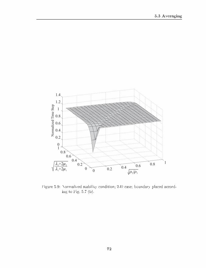
5.3 Averaging
0 0.2 0.4 0.6 0.8 1
� �2 1/0
0.20.4
0.60.8
1
� �� �
2 2
1 1
+2
+2
0
0.2
0.4
0.6
0.8
1
1.2
1.4
No
rmal
ized
Tim
eS
tep
Figure 5.9: Normalized stability condition; 2-D case; boundary placed accord-ing to Fig. 5.7 (b).
72

5.3 Averaging
� �2 1/
� �2 1/
� �2 1/
No
rmal
ized
Tim
eS
tep
No
rmal
ized
Tim
eS
tep
No
rmal
ized
Tim
eS
tep
0 0.2 0.4 0.6
c c2 1/ = 2
0.2
0
1.4
0.4
0.6
0.8
1
1.2
0 0.2 0.4 0.6 0.8 1
c c2 1/ = 1
0.2
0
1.4
0.4
0.6
0.8
1
1.2
0 0.2 0.4 0.6 0.8 1 1.2
1.2c c2 1/ = 0.5
1-D Lower Bound
1-D Not Averaged
2-D Boundary A
2-D Boundary B
2-D Averaged0.2
0
1.4
0.4
0.6
0.8
1
1.2
Figure 5.10: Comparison of 1-D and 2-D stability behavior; four velocity ratios.
73

5.3 Averaging
tween two di�erent media. The �eld components in x and z are labeled by i and j,
respectively. The boundary between the two media is placed such that the normal
particle velocity components are located on the interface. Thus, Vx is placed on a
vertical boundary, whereas Vz is placed on a horizontal boundary. The only stress
component, in that case, that lies on the boundary is the shear stress Txz. First the
procedure for averaging the material density in the equation of motion is derived,
then the averaging of the shear sti�ness � is explained.
5.3.1 Material Density
The procedure for averaging the material density on the boundary is derived from
the equation of motion. The derivation of the averaging is analogous for both the
horizontal and vertical boundary and, thus, the averaging procedure is presented only
for the horizontal particle velocity on a vertical interface. The equation of motion,
r � � = �@v
@t; (5.45)
is expanded for the 2-D Shear-Vertical (S-V) case in the x-z plane:
@
@x�xx +
@
@z�xz = �
@vx@t
(5.46)
@
@x�xz +
@
@z�zz = �
@vz@t
: (5.47)
The only non-zero velocity components are vx and vz. Considering the horizontal
particle velocity vx, the procedure for averaging the material density on the vertical
boundary is derived by integrating Eq. (5.46) over a box enclosing a portion of the
boundary as depicted in Fig. 5.12:
ZZBox
"@
@x�xx +
@
@z�xz
#dx dz =
I(�xxx+ �xzz) n ds =
ZZBox
�@vx@t
dx dz; (5.48)
where the density � is a function of position, and Gauss' integral theorem has been
applied to convert the surface integral on the left hand side into a contour integral;
74

5.3 Averaging
z
x
i�1 i i+1
j+1
j�1
j
Medium 2Medium 1
Figure 5.11: Boundary between two media in a 2-D �nite-di�erence grid; thenormal particle velocities and the shear stress are located on theinterface.
75

5.3 Averaging
z
x
� ��A��
� ��A��
�x
�z
i
j�1
j
Medium 2Medium 1
n
n
Vx
Txz
T , Txx zz
Figure 5.12: Averaging of the material density �; the normal stress componentsare integrated along the contour.
n is the normal vector to the contour, and x and z are normal vectors in the x- and
z-direction, respectively.
Using the discrete �nite-di�erence formulation, the integration is carried out over
a box of area �A = �x ��z, equivalent to the size of one cell of the �nite-di�erencegrid (see Fig. 5.12). Assuming the boundary between Medium 1 and Medium 2 divides
the area of integration in half, the integral comes out to be
�1 + �22
�A � Vk+0:5x ji;j�0:5 � V k�0:5
x ji;j�0:5�t
=
�T kxxji+0:5;j�0:5 � T k
xxji�0:5;j�0:5���z +
+�T kxzji;j � T k
xzji;j�1���x: (5.49)
After dividing by �A, the �nite-di�erence approximation to Eq. (5.46) is obtained:
�1 + �22
� Vk+0:5x ji;j�0:5 � V k�0:5
x ji;j�0:5�t
=
76
5.3 Averaging
T kxxji+0:5;j�0:5 � T k
xxji�0:5;j�0:5�x
+
+T kxzji;j � T k
xzji;j�1�z
: (5.50)
Thus, for the velocity components on the boundary, the material densities of the two
media are averaged arithmetically:
�avg = (�1 + �2)=2: (5.51)
The same result is obtained for the vertical particle velocity on a horizontal interface.
5.3.2 Lam�e's Constants
The procedure for averaging Lam�e's constants for the stress components on the bound-
ary is derived by using the elastic constitutive relation together with the strain-
velocity relation. The elastic constitutive relation combines the mechanic strain and
the stress and is usually expressed as
� = c � S; (5.52)
where the stress � and the strain S are 3� 3 tensors and the sti�ness matrix c is a
four-dimensional tensor of size 3�3�3�3. For an isotropic and lossless medium, the
entries of the sti�ness matrix are completely described by two independent constants,
Lam�e's constants � and �.
In the 2-D �nite-di�erence gird (Fig. 5.11), the shear stress Txz is placed on the
boundary and, consequently, Lam�e's constants are averaged for only Txz. By combin-
ing the strain-velocity relation and the constitutive relation, an equation relating vx
and vz to �xz arises, from which, in the �nite-di�erence formulation, the shear stress
is determined:@vx@z
+@vz@x
=1
�
@�xz@t
: (5.53)
77

5.3 Averaging
The averaging of � is achieved by integrating over a box enclosing parts of the bound-
ary, and Eq. (5.53) becomesZZBox
"@vx@z
+@vz@x
#dx dz =
ZZBox
1
�
@�xz@t
dx dz: (5.54)
Fig. 5.13 shows the integration contour around �xz. Applying Stoke's integral theorem,
the left hand side of Eq. (5.54) can be written asZZBox
"@vx@z
+@vz@x
#dx dz =
ZZBox
r� (vx � x� vz � z) ~dA =I(vx � x� vz � z) ~ds:
(5.55)
z
x
� ��A ��� ��A �
�
�x
�z
i
j-1ds
Vx
Vz
Txz
Figure 5.13: Averaging of the shear sti�ness �; the tangential velocity compo-nents are integrated along the contour.
Using the discrete �nite-di�erence formulation and Eq. (5.55), Eq. (5.54) be-
comes
�V k+0:5x ji;j�0:5 � V k+0:5
x ji;j�1:5���x+
�V k+0:5z ji+0:5;j�1 � V k+0:5
z ji�0:5;j�1���z
=�A
2
1
�1+
1
�2
!T k+1xz ji;j�1 � T k
xzji;j�1�t
: (5.56)
78

5.4 The Courant Condition
Thus, the inverse of the shear sti�ness � is averaged on the boundary between two
media as1
�avg=
1
2
1
�1+
1
�2
!: (5.57)
The same is obtained for the �eld components on a horizontal boundary. For the
shear stress on a corner of the boundary (i. e., Txz(i; j) in Fig. 5.11), the integration
yields1
�avg=
1
4
3
�1+
1
�2
!: (5.58)
5.4 The Courant Condition
By analyzing the eigenvalues of A (see Eq. (5.15)) for a homogeneous material, it can
be shown that the Courant condition itself is only a bound on the stability and can
be exceeded. For a homogeneous medium with wave speed c and density �, A can be
written as
A =
266666666666666664
. . . . . .
. . . 2� 2�t2
�x2c2 �t2
�x2c2 0
�t2
�x2c2 2� 2�t2
�x2c2 �t2
�x2c2
0 �t2
�x2c2 2� 2�t2
�x2c2
. . .
. . . . . .
377777777777777775
; (5.59)
where A has size N�N . The eigenvalues of this matrix can be determined explicitly:
�A = 2� 2�t2
�x2c2 + 2
�t2
�x2c2 cos(
p�
N + 1); (5.60)
where p = 1 : : :N and j�Aj � 2 for the system to be stable. The Courant condition is
obtained by assuming the smallest possible value for the cosine, i. e., �1. However,from Eq. (5.60) it becomes clear that the cosine will never become �1, because the
79

5.5 Concluding Remarks
argument of the cosine will never reach �. Only in the limit as N goes to in�nity
the argument of the cosine will approach � for k = N , and the cosine will become
�1. However, if for example N = 5, in the worst case cos(5�6) = �0:8660, and the
stability condition becomes
2� 2�t2
�x2c2(1 + 0:8660) � �2;
and from this�t2
�x2c2 � 2
1:8660= 1:0718: (5.61)
Thus, the time step can be chosen larger than dictated by the Courant condition.
Obviously, this observation is of only theoretical value, because actual problem
dimensions will never be small enough for this observation to be relevant. For exam-
ple, if N = 50, the factor by which the Courant condition can be exceeded reduces
to 1:0004.
5.5 Concluding Remarks
The type of instabilities described in this section are not limited to only the FDTD
algorithm for elastodynamics. Due to the similar structure of the FDTD algorithm,
the same e�ects will also be observed in electromagnetics at a material interface
with greatly di�erent properties, but can be avoided if the material parameters are
averaged on the boundary.
80

CHAPTER 6
Elastic Surface Waves
Elastic surface waves have been the object of extensive research, since Lord Rayleigh
�rst discovered the existence of elastic waves con�ned to the super�cial region of an
in�nite homogeneous isotropic solid more than a century ago [66]. Elastic surface
waves play an important role in various �elds. In seismology, surface waves have
been found to carry the bulk of the energy among the waves excited by an earth-
quake. In electroacoustics, surface waves are utilized to make �lters and resonators.
In geoscience, the propagation characteristics of surface waves are used to obtain in-
formation about the physical properties of the ground. In this chapter, the theory of
elastic surface waves is revisited.
A point source that is placed on the surface of a homogeneous isotropic medium
excites �ve di�erent kinds of waves: a pressure wave and a shear wave propagating in
the medium, a Rayleigh surface wave that is con�ned to the surface of the medium, a
lateral wave that is induced by the pressure wave at the surface, and a leaky surface
wave that travels along the surface with a wave speed smaller than the pressure wave
but larger than the shear wave. The �rst four of these wave types are well-known and
have been treated extensively in the literature. However, the existence and theoretical
foundation of the leaky surface wave has not been discussed much.
The leaky surface wave arises from the complex conjugate roots of the Rayleigh
equation. The leaky surface wave is an inhomogeneous wave that propagates along
the surface with a phase velocity larger than the shear wave but smaller than the
81

6.1 The Rayleigh Equation
pressure wave. It couples into a plane shear wave that propagates in the medium.
Due to the coupling, the surface wave loses energy and, thus, decays in its propagation
direction.
The leaky surface wave has been observed by various authors in experimental
and numerical studies. For example, Roth et al. noticed a rapidly decaying seismic
surface wave in an environment with a very high Poisson ratio that had a phase
velocity larger than the Rayleigh wave, but smaller than the pressure wave [67].
Smith et al. identi�ed prograde and retrograde surface wave modes in a geologic
study conducted on the shore of the gulf of Mexico [68]. And Glass and Maradudin
found a leaky surface wave to exist in the at-surface limit of a corrugated crystal
surface [69].
In this chapter, the theoretical derivation of the leaky surface wave is described.
In Sec. 6.1, the governing equations are brie y outlined, leading to the Rayleigh
equation. The derivation of the Rayleigh equation is adopted from Gra� [58] and is
described for the sake of completeness. In Sec. 6.2, the various roots of the Rayleigh
equation are discussed. It will be shown that for materials with a high Poisson ratio a
leaky surface wave exists, due to the complex conjugate roots of the Rayleigh equation.
In Sec. 6.3, the waves excited by a line source on the surface are derived analytically.
The method of steepest descent is applied to obtain closed-form expressions for the
various waves in the far �eld. The line-source case has been treated by many authors
[70] { [72]. The procedure that is described here closely follows Felsen and Marcuvitz
[73] and is mainly aimed at showing that a leaky surface wave is excited by a source
on the surface. The asymptotic expressions for all other wave types in the far �eld
are well-known and are given only for completeness reasons.
6.1 The Rayleigh Equation
The elastic wave �elds at the surface of a semi-in�nite, isotropic, lossless, homogeneous
half space are to be determined. The half-space is bounded at z = 0 by a free-surface
82

6.1 The Rayleigh Equation
boundary. The �elds are assumed to be invariant in the y-direction and non-zero
only in the x-z plane (plane-strain case, uy = @=@y = 0). Thus, the originally three-
dimensional problem reduces to a two-dimensional one.
The elastic wave �elds in a medium may be expressed in terms of their potential
functions [58]:
u = r � � +r�H; (6.1)
where u is the displacement vector, � is a scalar potential describing the longitudinal
pressure wave, and H is a vector potential describing the transverse shear wave. The
potentials satisfy the wave equations
r2� =1
c2P
@2�
@t2(6.2)
r2H =1
c2S
@2H
@t2; (6.3)
for the pressure and shear wave, respectively, with their corresponding wave speeds,
cP and cS. In the plane-strain case, the only non-zero vector potential component is
Hy, and the only non-zero displacement components are ux and uz:
ux =@�
@x� @Hy
@z(6.4)
uz =@�
@z+@Hy
@x: (6.5)
The only independent stress components are �xx, �zz, and �xz. The stresses are ex-
pressed in terms of the displacements as
�xx = (�+ 2�)@ux@x
+ �@uz@z
(6.6)
�yy = �
@ux@x
+@uz@z
!(6.7)
�zz = �@ux@x
+ (�+ 2�)@uz@z
(6.8)
�xz = �
@ux@z
+@uz@x
!: (6.9)
83

6.1 The Rayleigh Equation
Note that �yy is non-zero, but is dependent on �xx and �zz and can be written as:
�yy =�
2�+ 2�(�xx + �zz) : (6.10)
Introducing the potentials, the stresses become
�xx = (�+ 2�)@2�
@x2+ �
@2�
@z2� 2�
@2Hy
@x@z(6.11)
�zz = �@2�
@x2+ (�+ 2�)
@2�
@z2+ 2�
@2Hy
@x@z(6.12)
�xz = �
2@2�
@x@z� @2Hy
@z2+@2Hy
@x2
!: (6.13)
Assuming harmonic time-dependence, the plane wave solutions for � and Hy
satisfying Eqs. (6.2) and (6.3) are given by
� = Aej�x+j�z�j!t (6.14)
Hy = Bej�x+j�z�j!t; (6.15)
and the wave numbers are de�ned by
�2 = !2=c2P � �2 (6.16)
�2 = !2=c2S � �2 (6.17)
�2 = !2=c2: (6.18)
Inserting Eqs. (6.14) and (6.15) into Eqs. (6.4){(6.5) and (6.11) { (6.13), the displace-
ment and stress components are obtained:
ux =�j�Aej�z � j�Bej�z
�ej�x (6.19)
uz =�j�Aej�z + j�Bej�z
�ej�x (6.20)
�xx = ��(2�2 � �2 � �2)Aej�z + 2��Bej�z
�ej�x (6.21)
84

6.1 The Rayleigh Equation
�zz = ��(�2 � �2)Aej�z � 2��Bej�z
�ej�x (6.22)
�xz = ���2��Aej�z + (�2 � �2)Bej�z
�ej�x: (6.23)
Eqs. (6.19){(6.23) describe the wave �elds that are comprised of two and only
two wave components: one pressure wave component, de�ned by its potential function
� (according to Eq. (6.14)) with the wave number � and the amplitude A, and one
shear wave component, characterized by its potential function Hy (Eq. (6.15)) with
the wave number � and the amplitude B. By applying the appropriate boundary
conditions to Eqs. (6.19){(6.23), the waves that arise at the free surface and that
can be described by the two components are obtained. As a consequence, multiple
re ected waves that arise from an incident wave due to mode conversion at the surface
will not be part of the solution, because the multiple re ected waves are de�ned by
more than two components. For example, in general a plane pressure wave that is
incident on the surface at an angle � will give rise to both a re ected pressure wave
and a re ected shear wave. However, three wave components with three distinct wave
numbers and amplitudes are necessary to describe this scenario, and therefore this
case will not be a solution to Eqs. (6.19){(6.23).
At the surface, the normal stress vanishes, and thus �zzjz=0 = �xzjz=0 = 0. Using
this condition, the ratio of the coeÆcients is determined from Eqs. (6.22) and (6.23)
to beA
B=
2��
�2 � �2= ��
2 � �2
2��: (6.24)
Re-inserting the amplitude ratio into Eqs. (6.22) and (6.23), the frequency equation
is obtained:
(�2 � �2)2 + 4�2�� = 0: (6.25)
Eq. (6.25) is commonly called the Rayleigh Equation, because it gives rise to the
well-known Rayleigh surface wave.
Using Eqs. (6.16){(6.18), the frequency equation can be rewritten in terms of
85
6.2 The Roots of the Rayleigh Equation
the wave speeds: 2� c2
c2S
!2+ 4
sc2
c2P� 1
sc2
c2S� 1 = 0: (6.26)
By rationalizing, this equation may be expressed as
�c
cS
�2 " � c
cS
�6� 8
�c
cS
�4+�24� 16(cS=cP )
2�� c
cS
�2�
� 16�1� (cS=cP )
2� #
= 0: (6.27)
Eq. (6.27) always has three solutions for c2 (when neglecting the trivial solution).
Dependent on the Poisson Ratio � of a material, di�erent kinds of roots arise. For
� > 0:263, Eq. (6.27) has one real root and two complex conjugate roots. For � <
0:263, Eq. (6.27) has three real roots. In each case, the real root that is smallest in
magnitude gives rise to the Rayleigh surface wave, which propagates along the surface
and decays into the medium. The other roots have often been classi�ed as erroneous
or non-physical roots of the Rayleigh equation. However, it will be shown here that
the complex conjugate roots of the Rayleigh equation for � > 0:263 in fact give rise
to a leaky surface wave and the two additional real roots for � < 0:263 describe the
angles of incidence at which complete mode conversion occurs at the surface.
6.2 The Roots of the Rayleigh Equation
Let the roots of Eq. (6.27) be denoted by c. In general, c will be complex:
c = cr + jci; (6.28)
where cr is the real part and ci is the imaginary part of c. If c is purely real (c = cr),
� will be real (see Eq. (6.18)). If additionally c is smaller than both the pressure
wave speed and the shear wave speed, i. e., c = cr < cS < cP , � and � will be purely
imaginary. For the solution to be physical, Imf�g = �i > 0 and Imf�g = �i > 0,
thus the waves described by these wave numbers propagate in the x-direction and
decay in the z-direction. This solution represents the well-known Rayleigh surface
86

6.2 The Roots of the Rayleigh Equation
wave, �rst explored by Lord Rayleigh more than a century ago [66]. A solution of
this form always exists, independent of the Poisson ratio of a material.
6.2.1 Materials with a Poisson Ratio larger than 0.263
If � > 0:263, a real root and two complex conjugate roots of the Rayleigh equation
arise. The real root gives rise to the Rayleigh surface wave. For the complex conjugate
roots, the wave speed is complex, c = cr+jci, and consequently also the wave numbers
are complex: � = �r + j�i, � = �r + j�i and � = �r + j�i. It can be shown that for
the complex conjugate roots the real part of the wave speed is always smaller than
the pressure wave speed, but larger than the shear wave speed, cS < Refcg < cP .
Although c may be a solution to Eq. (6.27), it does not necessarily follow that
also Eq. (6.25) is ful�lled. This is due to the manipulation of Eq. (6.25) to arrive
at Eq. (6.27). In fact, the complex conjugate roots of Eq. (6.27) do not represent
solutions to Eq. (6.26). It can be shown, however, that they do represent solutions
to Eq. (6.25), if the signs of the wave numbers � and � are picked correctly. It may
be recalled that according to Eqs. (6.16) and (6.17) the wave numbers � and � are
functions of the square root of c2,
� = �!c
sc2
c2P� 1 = �(�r + j�i) (6.29)
� = �!c
sc2
c2S� 1 = �(�r + j�i): (6.30)
The sign in front of the square roots must be chosen according to physical and causal
constraints of the underlying problem. To obtain Eq. (6.26), the positive sign has been
assumed for both � and �. However, it turns out that Eq. (6.25) is only satis�ed if,
for the complex conjugate roots, both the real part and the imaginary part of � and
� have opposite signs, i. e., sign(�r) 6= sign(�r) and sign(�i) 6= sign(�i).
Fig. 6.1 schematically shows the arrangement of the roots in the complex �-
plane. The possible solutions of the Rayleigh equation are summarized in Table 6.1,
giving all possible combinations of �, � and �. Only waves propagating in the positive
87

6.2 The Roots of the Rayleigh Equation
x-direction are considered. Five possible solutions arise. The �rst solution describes
kP kSRe{ }�
Im{ }�
Complex Conjugate Roots
Rayleigh Wave Root
Figure 6.1: Schematical arrangement of the roots in the complex �-plane for� > 0:263.
the Rayleigh surface wave. For the second solution, both the pressure wave potential
and the shear wave potential, � and Hy, propagate and increase in the positive
x-direction (�r > 0, �i < 0). However, � propagates and decays in the positive
z-direction (�r > 0, �i > 0), whereas Hy propagates and decays in the negative
z-direction (�r < 0, �i < 0). For the third solution, the potentials decay in the
x-direction (�i > 0). � now propagates and increases in the negative z-direction
(�r < 0, �i > 0), whereas Hy propagates and increases in the positive z-direction
(�r > 0, �i < 0). For the fourth and �fth solution, the signs of � and � are reversed.
The behavior of the �ve possible solutions is best demonstrated by calculating
the wave �elds for a medium with a speci�c value of Poisson's ratio. Assuming
Poisson's ratio to be � = 0:4, the elastic wave �elds are computed using Eqs. (6.19){
(6.23). The amplitude of the shear wave potential is chosen to be unity, and the
amplitude of the pressure wave potential is computed with Eq. (6.24). For � = 0:4,
88

6.2 The Roots of the Rayleigh Equation
Table 6.1: Solutions to the Rayleigh equation for � > 0:263.
(1) �r > 0, �i = 0 �r = 0, �i > 0 �r = 0, �i > 0
� � e�j�ijzejj�rjx Hz � e�j�ijzejj�rjx
(2) �r > 0, �i < 0 �r > 0, �i > 0 �r < 0, �i < 0
� � e(jj�rj�j�ij)ze(jj�rj+j�ij)x Hz � e(�jj�rj+j�ij)ze(jj�rj+j�ij)x
(3) �r > 0, �i > 0 �r < 0, �i > 0 �r > 0, �i < 0
� � e(�jj�rj�j�ij)ze(jj�rj�j�ij)x Hz � e(jj�rj+j�ij)ze(jj�rj�j�ij)x
(4) �r > 0, �i < 0 �r < 0, �i < 0 �r > 0, �i > 0
� � e(�jj�rj+j�ij)ze(jj�rj+j�ij)x Hz � e(jj�rj�j�ij)ze(jj�rj+j�ij)x
(5) �r > 0, �i > 0 �r > 0, �i < 0 �r < 0, �i > 0
� � e(jj�rj+j�ij)ze(jj�rj�j�ij)x Hz � e(�jj�rj�j�ij)ze(jj�rj�j�ij)x
the pressure wave speed exceeds the shear wave speed by a factor of about 2.45:
cP = 2:4495cS. The roots of Eq. (6.27) in terms of the shear wave speed cS are
c =
8>>>>><>>>>>:
0:9422cS
(1:9276 + j0:3996)cS
(1:9276� j0:3996)cS
: (6.31)
The resulting wave numbers are shown in Table 6.2. All wave numbers are expressed
in terms of the longitudinal wave number, kP = !=cP .
In Fig. 6.2, the displacements according to the �ve solutions of the Rayleigh
equation are plotted versus x and z. The distance on the axes is normalized to the
wave length of the Rayleigh surface wave, �R. The upper edge of each plot corre-
sponds to the surface. The two columns show the horizontal and vertical displace-
ments, ux and uz. Pseudo-color plots are used to display the wave �elds, employing a
logarithmic scale with a dynamic range of 50 dB. Superimposed with the horizontal
displacement component is the real part of the complex Poynting vector, thus indi-
cating the direction of the energy ow. The complex Poynting vector is de�ned as
89

6.2 The Roots of the Rayleigh Equation
Table 6.2: Solutions to the Rayleigh equation for � = 0:4: wave numbers.
� = � = � =
(1) 2:5998kP j2:3997kP j0:8711kP
(2) (1:2184 � j0:2526)kP (0:4030 + j0:7636)kP (�2:1448 � j0:1435)kP
(3) (1:2184 + j0:2526)kP (�0:4030 + j0:7636)kP (2:1448 � j0:1435)kP
(4) (1:2184 � j0:2526)kP (�0:4030 � j0:7636)kP (2:1448 + j0:1435)kP
(5) (1:2184 + j0:2526)kP (0:4030 � j0:7636)kP (�2:1448 + j0:1435)kP
[57]
P =j!u � � �
2; (6.32)
where the star denotes the complex conjugate. The real part of the complex Poynting
vector describes the average power per unit area.
First, the Rayleigh surface wave is shown. For the Rayleigh surface wave, the
energy ow is seen to be parallel to the surface. Both the horizontal and the vertical
displacements decay away from the surface. The second solution describes a shear
wave in which energy is carried towards the surface. Close to the surface, the energy
ows parallel to the surface. The waves grow exponentially in the x- and z-direction.
The third solution is the converse of the second one. This time, the energy ows from
the surface into the medium, and the waves decay in the x-direction. Again, close to
the surface the energy ow is parallel to the surface. The fourth and �fth solution
are similar to the second and third. However, now a pressure wave propagates in the
medium, and the energy ows at a di�erent angle with respect to the surface. Also,
the exponential growth is enhanced.
All of the �ve possible solutions described above can, in certain cases, represent
physical solutions. For example, if a �eld distribution is created on the surface that
matches the �eld distribution of Solution (5) on the surface, waves similar to the ones
described by Solution (5) will be induced in the medium. If a �eld distribution is
90

6.2 The Roots of the Rayleigh Equation
00
.51
1.5
22
.5
0 1
0 0.5 1 1.5 2 2.5-1
1
-2 4
00
.51
1.5
22
.5
-10
10
0 0.5 1 1.5 2 2.5
-2 4
00
.51
1.5
22
.5
-2
1
0 0.5 1 1.5 2 2.5
-100 0
00
.51
1.5
22
.5
-10
10
0 0.5 1 1.5 2 2.5
00.5
11.5
22.5
0
100
0 0.5 1 1.5 2 2.5-1
2
ux uz
ux
uz
x/�R
z/�R(1)
(2)
(3)
(4)
(5)
Figure 6.2: Horizontal and vertical displacements according to the �ve solutionsof the Rayleigh equation.
91

6.2 The Roots of the Rayleigh Equation
generated within the medium that is equal to the �eld distribution of Solution (2),
waves propagating towards the surface will be excited that perfectly couple into a
surface wave. Of course, the solutions as described here would require an in�nite
medium and wave �elds of in�nite extent that are non-zero at in�nity, which violates
physical as well as causal constraints. However, over a �nite range all of these solutions
can be excited with the appropriate �eld distributions on the boundaries.
Interpretation in the k-Space
Further physical insight can be gained by looking at the wave vectors for the solutions
in the k-space. The wave vectors in the k-space will lie on well-de�ned surfaces, the
allowed wave-vector surfaces. By looking at the allowed wave-vector surfaces, the
coupling between the surface waves and the waves in the medium can be explained.
Fig. 6.3 shows the allowed wave vector surfaces for the pressure wave and the
shear wave in the kx-kz-plane. For the wave vector surfaces, the wave number of the
pressure wave and the shear wave in the z-direction, � and � according to Eqs. (6.16)
and (6.17), are plotted as a function of the wave number in the x-direction, �. The
allowed wave vector surfaces for the pressure and the shear wave are circles with radii
kP and kS, respectively. The allowed wave vector surfaces de�ne the wave vectors that
describe physical waves. The wave vectors indicate the propagation direction of the
waves and are inversely proportional to their wave speed. In Fig. 6.3, the wave vectors
of the surface waves that arise from the Rayleigh equation are indicated by the bold
solid arrows along the kx-axis. The gray arrow corresponds to the real part of the
wave vector of the Rayleigh surface wave according to Solution (1), whereas the black
arrow describes the real part of the wave vector in the x-direction of Solutions (2) {
(5).
From the wave vectors in the k-space, conclusions about the coupling between
the di�erent waves can be drawn. At the surface, two waves will be coupled, if their
wave vector components tangential to the surface match both in the real part and the
imaginary part. The roots of the Rayleigh equation give rise to two di�erent kinds
92

6.2 The Roots of the Rayleigh Equation
k
kx=Re{ }�
kz
Re{ }�
Re{ }
kP
kS
Figure 6.3: Allowed wave vector surfaces in the k-space for the pressure wave(�) and the shear wave (�); lossless case.
of surface waves: the Rayleigh surface wave, described by Solution (1), and leaky
surface waves, described by Solutions (2) { (5). The surface waves are de�ned by
their wave vectors, which will be parallel to the kx-axis and, thus, tangential to the
surface. If the wave vector of a surface wave matches the projection onto the surface
of the wave vector describing a wave propagating in the medium, the two waves will
be coupled. The Rayleigh surface wave cannot be coupled to any wave propagating in
the medium. The wave number of the Rayleigh surface wave is larger than both the
wave number of the pressure wave, kP , and the wave number of the shear wave, kS,
and therefore the tangential wave vectors of the Rayleigh wave and a shear wave or a
pressure wave in the medium can never match. This is evident in Fig. 6.3: the wave
vector of the Rayleigh wave, indicated by the gray arrow, exceeds both kP and kS.
The wave number for the leaky surface wave, on the other hand, is larger than kP ,
but smaller than kS. Thus, there exists a shear wave that propagates in the medium
93

6.2 The Roots of the Rayleigh Equation
at such an angle that its tangential component matches the wave vector of the leaky
surface wave. This is shown in Fig. 6.3: the tangential wave vector components of
the shear waves described by the dashed arrows match the wave vector of the leaky
surface wave (solid arrow), and consequently the waves are coupled.
Fig. 6.3 describes the wave vector surfaces that arise when � is purely real. If �
is complex, the wave vector surfaces for the pressure and the shear wave will not be
circles, but they will be deformed. If � is real, the pressure wave number in the z-
direction, �, is purely real for jkxj < kP and purely imaginary for jkxj > kP . Similarly,
the shear wave number in the z-direction, �, is real for jkxj < kS and imaginary for
jkxj > kS. If � is complex, however, � and � will also both be complex. Speci�cally,
the real part of � and � will be non-zero for jkxj > kP and jkxj > kS, respectively. In
this case, a tangential wave vector match is possible between the leaky surface wave
and both a pressure wave and a shear wave.
Fig. 6.4 shows the wave vector surfaces that arise for Solutions (1) { (5). Except
for Solution (1), which describes the Rayleigh wave, the wave vector surfaces are de-
formed due to � being complex. For the Rayleigh wave (Solution (1)), � is purely real
and exceeds kP and kS, whereas � and � are both purely imaginary. The imaginary
parts of � and � both must be positive, because, due to physical constraints, the
Rayleigh wave must decay into the medium. Also in Fig. 6.4, the energy ow of the
Rayleigh wave in the x-z-plane is indicated schematically. For the Rayleigh wave,
the energy ows parallel to the surface, and the Rayleigh wave does not decay in
its propagation direction. Solutions (2) { (5) describe the leaky surface waves. For
Solution (2), a shear wave propagates towards the surface and couples into a surface
wave. Due to the coupling, both the surface wave and the shear wave in the medium
are inhomogeneous. The wave vectors of both the surface wave and the shear wave
in the medium are complex, and the allowed wave vector surfaces are deformed. The
surface wave has to components: a pressure wave component, which propagates and
decays into the medium, and a shear wave component, which propagates and decays
towards the surface. This is indicated by the wave vectors for the pressure and the
94

6.2 The Roots of the Rayleigh Equation
shear wave component (Solution (2), dashed arrows): the real and imaginary part of
� are positive, whereas the real and imaginary part of � are negative. In the medium,
the energy ows towards the surface. Close to the surface, the energy ow is parallel
to the surface. The surface wave grows exponentially in its propagation direction,
because it is constantly fed by the shear wave in the medium. For Solution (3), the
surface wave feeds a shear wave that propagates away from the surface. The surface
wave \leaks" energy into the medium. Consequently, the wave vector for the shear
wave component points into the medium. As for Solution (2), the shear wave in-
creases exponentially into the medium, indicated by the imaginary part of � being
negative. For Solutions (4) and (5), a pressure wave propagates in the medium. For
Solution(4), the pressure wave propagates and decays towards the surface, indicated
by the real and imaginary part of � being negative. For Solution (5), the pressure
wave is fed from the surface wave and propagates into the medium. In this case, the
real part of � is positive, and the imaginary part is negative.
6.2.2 Materials with a Poisson Ratio smaller than 0.263
For � < 0:263, three purely real roots of the Rayleigh equation exist. The root
smallest in magnitude gives rise to the Rayleigh surface wave. For the additional two
roots, the phase speeds along the surface are larger than the pressure wave speed, cP .
Thus, their wave numbers both in the x- and the z-direction are real and smaller in
magnitude than the wave number of the pressure wave speed, kP . The arrangement
of the roots in the complex �-plane is shown schematically in Fig. 6.5. The possible
solutions of the Rayleigh equation are summarized in Table 6.3, giving all possible
combinations of �, � and �. Except for the Rayleigh wave (Solution (1)), all wave
numbers are purely real, and therefore their imaginary part is zero. Only waves
propagating in the positive x-direction are considered. Five possible solutions arise.
The �rst solution again describes the Rayleigh surface wave. The other four solutions
depict cases of complete mode conversion for a plane wave incident on the surface.
95

6.2 The Roots of the Rayleigh Equation
k
kx=Re{ }�
kz
Re{ }�Im{ }�
Re{ }
Im{ }
kP
kS
x
z
Rayleigh
Solution (1)
Figure 6.4: Allowed wave vector surfaces for the �ve solutions to the Rayleighequation.
96

6.2 The Roots of the Rayleigh Equation
k
kx=Re{ }�
kz
Re{ }�
Im{ }�
Re{ }
Im{ }
kP
kS
x
z Shear
Solution (2)
k
kx=Re{ }�
kz
Re{ }�
Im{ }�
Re{ }
Im{ }
kP
kS
x
z Shear
Solution (3)
Figure 6.4: continued.
97

6.2 The Roots of the Rayleigh Equation
k
kx=Re{ }�
kz
Re{ }�
Im{ }�
Re{ }
Im{ }
kP
kS
x
z
Pressure
Solution (4)
k
kx=Re{ }�
kz
Re{ }�
Im{ }�
Re{ }
Im{ }
kP
kS
x
z
Pressure
Solution (5)
Figure 6.4: continued.
98

6.2 The Roots of the Rayleigh Equation
kP kSRe{ }�
Im{ }�
Rayleigh Wave Root
Real Roots
Figure 6.5: Schematical arrangement of the roots in the complex �-plane for� < 0:263.
Complete mode conversion occurs for both pressure waves and shear waves at certain
angles of incidence. At these angles of incidence, a plane shear wave, for example,
will be re ected solely as a plane pressure wave, and, thus, the shear wave mode
is completely converted into a pressure wave mode. The angles of incidence are
dependent on Poisson's ratio. Complete mode conversion is physically possible only
for materials with a Poisson ratio smaller than 0.263, i. e., if the Rayleigh equation has
three real roots. The second solution in Table 6.3 describes a shear wave incident on
the surface that completely couples into a re ected pressure wave. The third solution
describes the converse case: an incident pressure wave is completely converted into a
re ected shear wave. The fourth and �fth solution have the same shape as the second
and third solution, but are for di�erent angles of incidence.
The three real roots for a material with a Poisson ratio of � = 0:2 in terms of
99

6.2 The Roots of the Rayleigh Equation
Table 6.3: Solutions to the Rayleigh equation for � < 0:263.
(1) �r > 0 �i > 0 �i > 0
� � e�j�ijzejj�rjx Hz � e�j�ijzejj�rjx
(2) �r > 0 �r > 0 �r < 0
� � ejj�rjzejj�rjx Hz � e�jj�rjzejj�rjx
(3) �r > 0 �r < 0 �r > 0
� � e�jj�rjzejj�rjx Hz � ejj�rjzejj�rjx
(4) �r > 0 �r > 0 �r < 0
� � ejj�rjzejj�rjx Hz � e�jj�rjzejj�rjx
(5) �r > 0 �r < 0 �r > 0
� � e�jj�rjzejj�rjx Hz � ejj�rjzejj�rjx
the shear wave speed are
c =
8>>>>><>>>>>:
0:9110cS
1:6398cS
2:1169cS
: (6.33)
For � = 0:2, the pressure wave speed exceeds the shear wave speed by a factor of
1.63: cP = 1:6330cS. Table 6.4 shows the wave numbers arising from the three real
roots.
The solutions due to the real roots are best illustrated by plotting the resulting
wave �elds due to an excitation in the time domain rather than for harmonic time
dependence. For this, the wave �elds are computed using Eqs. (6.19){(6.23), are
Fourier transformed into the time-domain and convolved with a speci�c time-domain
excitation. A di�erentiated Gaussian pulse with a center frequency of 400 Hz is
used. The results are shown in Fig. 6.6. The magnitude of the displacement �elds
according to the four solutions arising from the two additional real roots are plotted.
A logarithmic color scale with a dynamic range of 40 dB is used. Shear waves are
labeled by S and pressure waves by P. The bold gray arrows indicate the propagation
100

6.3 Waves due to a Line Source on the Surface
Table 6.4: Solutions to the Rayleigh equation for � = 0:2: wave numbers.
� = � = � =
(1) 1:7925kP j2:3997kP j0:8711kP
(2) 0:9959kP 0:0909kP �1:2942kP
(3) 0:9959kP �0:0909kP 1:2942kP
(4) 0:7714kP 0:6363kP �1:4393kP
(5) 0:7714kP �0:6363kP 1:4393kP
direction of the plane waves. As indicated in Table 6.3, Solutions (2) and (4) describe
cases of complete mode conversion for an incident shear wave, whereas Solutions (3)
and (5) are for an incident pressure wave. The angle of incidence at which complete
mode conversion occurs can be determined easily from the wave numbers:
� = tan�1(�r=j�rj) (6.34)
for an incident pressure wave and
� = tan�1(�r=j�rj) (6.35)
for an incident shear wave.
6.3 Waves due to a Line Source on the Surface
In the previous section, the solutions to the wave equation at a free-surface boundary
have been described in a general form. In this section, the wave �elds due to a speci�c
excitation, a line source on the surface, are determined.
Fig. 6.7 shows the underlying geometry. A line source is placed on the surface
at x = 0 and extends into the y-direction. The line source excites the normal stress
component �zz. If harmonic time dependence is assumed, the displacement �elds due
101

6.3 Waves due to a Line Source on the Surface
S
P
S
P
S
P
S
P
(2)
(3)
(4)
(5)
Figure 6.6: Magnitude of the displacements according to the four solutions dueto the two additional real roots for � < 0:263.
102

6.3 Waves due to a Line Source on the Surface
to the line source can be written in form of an integral equation [58]:
ux(x; z) = � j
��
ZP 0
�
F0(�)
h�2��ej�z + (�2 � �2)ej�z
iej�xd� (6.36)
uz(x; z) = � j
��
ZP 0
�
F0(�)
h2�2ej�z + (�2 � �2)ej�z
iej�xd�; (6.37)
where
F0(�) = (�2 � �2)2 + 4�2�� (6.38)
is the Rayleigh equation. The amplitude of the excitation is assumed to be unity.
For the analysis in the following, a medium with a Poisson ratio larger than 0.263 is
assumed, and, thus, F0 has one real root and two complex conjugate roots.
R
x
z
Surface Line Source
Figure 6.7: Line source on the surface.
6.3.1 General Considerations
The integrals in Eqs. (6.36) and (6.37) each represent an inverse Fourier transform
from the wave-number domain into the spatial domain. The integrands contain poles
and branch points. The poles are due to the roots of the Rayleigh equation in the
denominator. The branch points arise because of the square-root dependence of �
103

6.3 Waves due to a Line Source on the Surface
and � on �. They are located at the roots of � and �, at kP = �(!=cP )2 and
kS = �(!=cS)2 (see Eqs. (6.16) and (6.17)).
To compute the integrals, contour integration in the complex �-plane must be
applied. The integration must be performed along the real �-axis. Fig. 6.8 shows
the location of the poles and branch points in the complex �-plane. To determine
the waves propagating in the positive x-direction, Eqs. (6.36) and (6.37) must be
integrated along the path P 0. The contour is closed at in�nity. Only the poles and
branch cuts for Ref�g > 0 are included in the integration contour (indicated by the
indentations of P 0), whereas the poles for Ref�g < 0 are excluded and, therefore, do
not contribute to the integral.
Due to the branch points, the integrands are not single-valued. To make the
integrands unique, a multi-sheeted Riemann surface for the �-plane is necessary, with
branch cuts providing the transition from one Riemann sheet to the other [73]. The
location of the branch cuts in general is arbitrary, but de�nes the disposition of those
regions in the complex �-plane in which, for example, Ref�g > 0 or Ref�g < 0.
Fig. 6.8 shows the top Riemann sheet for Eqs. (6.36) and (6.37). The signs of the
wave numbers on the top Riemann sheet must be chosen for physical and causal
reasons. The integration along the real axis determines the shear and pressure waves
excited by the line source. For the shear and the pressure waves to be causal, they
must propagate away from the source and vanish at in�nity. For this to be true, the
wave numbers along the real axis must be chosen such that Ref�g > 0, Imf�g > 0,
Ref�g > 0 and Imf�g > 0. It can be easily shown that in that case the wave numbers
in the entire second and fourth quadrant must behave in the same way. In the �rst
and third quadrant, the branch cuts must then be chosen such that Ref�g < 0,
Imf�g > 0, Ref�g > 0 and Imf�g < 0. This is true because � and � must be
continuous across the real axis. Thus, in the �rst and third quadrant, the pressure
wave potential propagates and increases in the negative z-direction, whereas the shear
wave potential propagates and increases in the positive z-direction. It is evident that
in the �rst quadrant of the top Riemann sheet the wave numbers behave as described
104
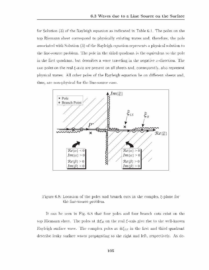
6.3 Waves due to a Line Source on the Surface
for Solution (3) of the Rayleigh equation as indicated in Table 6.1. The poles on the
top Riemann sheet correspond to physically existing waves and, therefore, the pole
associated with Solution (3) of the Rayleigh equation represents a physical solution to
the line-source problem. The pole in the third quadrant is the equivalent to the pole
in the �rst quadrant, but describes a wave traveling in the negative x-direction. The
two poles on the real �-axis are present on all sheets and, consequently, also represent
physical waves. All other poles of the Rayleigh equation lie on di�erent sheets and,
thus, are non-physical for the line-source case.
Im{ }�
Re{ }�
Re
Im
{ } < 0
{ } > 0
Re
Im
{ } > 0
{ } < 0
�
�
Re
Im
{ } > 0
{ } > 0
Re
Im
{ } > 0
{ } > 0
�
�
P’
�R�LS
Pole
Branch Point
Figure 6.8: Location of the poles and branch cuts in the complex �-plane forthe line-source problem.
It can be seen in Fig. 6.8 that four poles and four branch cuts exist on the
top Riemann sheet. The poles at ��R on the real �-axis give rise to the well-known
Rayleigh surface wave. The complex poles at ��LS in the �rst and third quadrant
describe leaky surface waves propagating to the right and left, respectively. As de-
105

6.3 Waves due to a Line Source on the Surface
scribed earlier, the leaky surface wave couples into a plane shear wave. Both the leaky
surface wave and the shear wave that is fed from the surface wave are inhomogeneous,
which is indicated by the pole being complex.
6.3.2 Steepest-Descent Approximation
To evaluate the integrals asymptotically in the far �eld, the method of steepest descent
shall be applied. To simplify the procedure, the two terms of the integral are treated
separately. Dividing the integrals each into a pressure wave term and a shear wave
term, Eqs. (6.36) and (6.37) are rewritten as
uSx(x; z) = � j
��
ZP 0
�
F0(�)(�2��)ej�zej�xd� (6.39)
uPx (x; z) = � j
��
ZP 0
�
F0(�)(�2 � �2)ej�zej�xd� (6.40)
uSz (x; z) = � j
��
ZP 0
�
F0(�)2�2ej�zej�xd� (6.41)
uPz (x; z) = � j
��
ZP 0
�
F0(�)(�2 � �2)ej�zej�xd�: (6.42)
The total displacements equal the superposition of the pressure wave component and
the shear wave component:
ux(x; z) = uSx(x; z) + uPx (x; z) (6.43)
uz(x; z) = uSz (x; z) + uPz (x; z): (6.44)
To facilitate the evaluation of the integrals, the complex �-plane is transformed
into the complex wS-plane for the two shear wave terms, and into the wP -plane for
the pressure wave terms. The transformations are de�ned by
� = kS sinwS (6.45)
� = kP sinwP : (6.46)
106

6.3 Waves due to a Line Source on the Surface
These transformations are single-valued [73]. From the periodicity of sinwS
and sinwP it is evident that multiple values for wS and wP correspond to a single
value of �. Thus, the transformations can be used to map the entire �-plane with
its multiple Riemann sheets into adjacent strips of width 2� in the wS- or wP -plane.
The arrangement of the poles and branch cuts of the top Riemann sheet in the
complex wS-plane and wP -plane are shown in Fig. 6.9. Here, the top Riemann sheet
is mapped into a strip reaching from �� to � in the complex wS-plane for the shear
wave terms, and similarly in the complex wP -plane for the pressure wave terms. The
positions of the transformed Rayleigh wave pole and the leaky surface wave pole in
the complex wS- and wP -plane are indicated by wSR, w
SLS, and wP
R, wPLS, respectively.
The transformed integration paths are denoted by P S and P P .
The separate transformations for the shear wave terms and the pressure wave
terms become necessary, because, when the method of steepest descent is applied,
the di�erent terms will give rise to di�erent steepest-descent paths. By applying
the di�erent transformations, the steepest-descent paths will have a rather simple
shape for both the shear wave terms and the pressure wave terms, thus, making the
steepest-descent approximation considerably easier.
Applying the transformations, two of the branch cuts are eliminated in each of
the integrals in Eqs. (6.39){(6.42). For the shear wave terms the branch cuts at �kSvanish, whereas for the pressure wave terms the branch cuts at �kP are removed. For
the shear wave terms, � then reduces to
� = kS coswS; (6.47)
and for the pressure wave terms � becomes
� = kP coswP : (6.48)
Introducing polar coordinates,
x = R sin � (6.49)
z = R cos �; (6.50)
107

6.3 Waves due to a Line Source on the Surface
Re{ }wS
Im{ }wS
��
-��
wRS
wLSS
PS
�= sinkS wS
(a)
Re{ }wP
Im{ }wP
��
-��
wRP
wLSP
PP
�= sinkP wP
(b)
Figure 6.9: Location of the poles and branch cuts (a) in the complex wS-planeand (b) in the complex wP -plane.
108

6.3 Waves due to a Line Source on the Surface
Eqs. (6.39){(6.42) are rewritten as integrals in the wS- and wP -plane:
uSx(x; z) = � j
��
ZPS
�
F0(�)(�2��)ejkSR cos(wS��)�dwS (6.51)
uPx (x; z) = � j
��
ZPP
�
F0(�)(�2 � �2)ejkPR cos(wP��)�dwP (6.52)
uSz (x; z) = � j
��
ZPS
�
F0(�)2�2ejkSR cos(wS��)�dwS (6.53)
uPz (x; z) = � j
��
ZPP
�
F0(�)(�2 � �2)ejkPR cos(wP��)�dwP ; (6.54)
where � describes the polar angle measured from the surface normal towards the
propagation direction (see Fig. 6.7). The wave numbers in terms of wS are
�(wS) = kS sinwS (6.55)
�(wS) = kS coswS (6.56)
�(wS) = �qk2P � �(wS)2 (6.57)
and in terms of wP
�(wP ) = kP sinwP (6.58)
�(wP ) = �qk2S � �(wP )2 (6.59)
�(wP ) = kP coswP : (6.60)
The signs of �(wS) and �(wP ) must be chosen as described earlier for the complex
�-plane. Thus, in the shaded and non-shaded regions of Fig. 6.9, � behaves just as in
the shaded and non-shaded regions of Fig. 6.8.
With the integrals transformed as described above, it is relatively straightfor-
ward to apply the method of steepest descent. For the method of steepest descent,
the integration paths P S and P P are deformed into new paths, the steepest-descent
109

6.3 Waves due to a Line Source on the Surface
paths �P S and �P P , respectively. The new path is chosen such that the dominant con-
tribution to the integral arises from only a small section of the path. To achieve this,
the path is deformed such that it passes through the saddle point of the integrand.
Away from the saddle point it follows the direction in which the integrand decays
most rapidly. Along this path, the integrand will then be negligible everywhere but
around the saddle point, and the integral can be approximated by the contribution
from the integrand in the vicinity of the saddle point.
The path of steepest descent is a path of constant phase [73]. For integrals in
the form of the ones in Eqs. (6.51){(6.54), the steepest-descent path is given by
RefwS;Pg � � = cos�1(sech(ImfwS;Pg)): (6.61)
The procedure is the same for the shear wave terms and the pressure wave terms. In
Fig. 6.10, three steepest-descent paths are shown each for the shear wave terms in
the wS-plane, �P S1 , �P
S2 , �P
S3 , and for the pressure wave terms in the wP -plane, �P P
1 , �PP2 ,
�P P3 . Each steepest descent path corresponds to a di�erent propagation (polar) angle.
The saddle point in each case is located at the intersection of the steepest-descent
path with the real wS- or wP -axis, respectively. Physically, the contributions from
the saddle points describe the pressure and the shear waves in the far �eld .
When the original integration path is deformed into the steepest-descent path,
care has to be taken whether poles or branch cuts are crossed during the deformation.
According to Cauchy's theorem, if a singularity is crossed during the deformation from
one integration path into another, the contribution from the contour integral around
the singularity must be included into the total integral. For example, when P S in
Fig. 6.10 is deformed into the steepest-descent path �P S1 , no singularities are crossed
during the deformation. However, for �P S2 , the integrals around the branch cut, �Pb,
and around the pole at wSR must be included. For �P S
3 , the branch cut integral as well
as the integrals around the poles at wSR and wS
LS contribute to the total integral.
The contour integrals around the singularities in both the wS- and the wP -plane
give rise to di�erent types of waves. The integral around the branch cut in the
110

6.3 Waves due to a Line Source on the Surface
Re{ }wS
Im{ }wS
�� -��
R
S
L
S
LS
S
PS
P1
S
Pb
P2
S P3
S
(a)
R
P
LS
P
P1P P2
P P3P
Re{ }wP
Im{ }wP
��
-��
PP
(b)
Figure 6.10: Steepest descent paths for (a) the shear wave terms in the complexwS-plane and (b) the pressure wave terms in the complex wP -plane.
111
6.3 Waves due to a Line Source on the Surface
wS-plane describes a lateral wave. The lateral wave is a plane shear wave induced
by the pressure wave propagating along the surface. It appears only if the polar
angle exceeds �SL = sin�1(kP=kS), because, mathematically, the branch cut integral
contributes to the total integral only for � > �SL. It can be shown that the integral
around the branch cut in the wP -plane is approximately zero and, thus, it does
not contribute to the total integral. The integrals around the poles give rise to
the Rayleigh surface wave and the leaky surface wave. They exist only for � > �SR
and � > �SLS in the wS-plane, and for � > �PR and � > �PLS in the wP -plane. The
total Rayleigh surface wave and the total leaky surface wave are comprised of the
superposition of the contributions from the integrals around the singularities both in
the wS-plane and wP -plane. The angles �S;PR and �S;PLS are easily obtained by inserting
wS;PR = sin�1(�R=kS;P ) and wS;P
LS = sin�1(�LS=kS;P ) into Eq. (6.61).
The integrals are now approximately determined using the method of steepest-
descent. Five separate wave types arise: the bulk shear wave, the bulk pressure
wave, the Rayleigh surface wave, the leaky surface wave and the lateral wave. A
detailed description of the steepest-descent method is given, for example, by Felsen
and Marcuvitz [73]. Using the method of steepest-descent, the shear wave in the far
�eld comes out to be
ux(R; �)jShear =j
��
s2�
kSR
ej(kSR��=4)
F0(kS sin �)�
� 2qk2P � k2S sin
2 � k3S sin � cos2 � (6.62)
uz(R; �)jShear =�j��
s2�
kSR
ej(kSR��=4)
F0(kS sin �)�
� 2qk2P � k2S sin
2 � k3S sin2 � cos �: (6.63)
For the pressure wave,
ux(R; �)jPressure =�j��
s2�
kPR
ej(kPR��=4)
F0(kP sin �)�
112

6.3 Waves due to a Line Source on the Surface
�hk2S � 2k2P sin
2 �ik2P sin � cos � (6.64)
uz(R; �)jPressure =�j��
s2�
kPR
ej(kPR��=4)
F0(kP sin �)�
�hk2S � 2k2P sin
2 �ik2P cos
2 �: (6.65)
The Rayleigh surface wave and the leaky surface wave are derived from the
contour integral around the respective poles of the Rayleigh equation. Using contour
integration, the Rayleigh wave is described by
ux(R; �)jRayleigh =2�R
�F 00j�R
hU(� � �SR) � (�2�R�R)ej�RR cos �
+U(� � �PR) � (�2R � �2R)ej�RR cos �
i� ej�RR sin � (6.66)
uz(R; �)jRayleigh =2�R�F 0
0j�RhU(� � �SR) � 2�2Rej�RR cos �
+U(� � �PR) � (�2R � �2R)ej�RR cos �
i� ej�RR sin �; (6.67)
where
F 00j�R = 4�R(�
2R � �2R) + 8�R�R�R � 4�3R
�R�R
+�R�R
!: (6.68)
F 00j�R is the derivative of the Rayleigh equation with respect to � at � = �R, and
U(� � �S;PR ) is the Heaviside unit step function; �R, �R, and �R describe the wave
numbers of the Rayleigh wave (see Table 6.2). The result for the leaky surface wave
is determined in exactly the same way and is obtained by simply replacing �S;PR , �R, �R
and �R by �S;PLS , �LS, �LS and �LS, i. e., inserting the wave numbers for the leaky-wave
pole instead of the Rayleigh wave pole.
The lateral wave is de�ned by the integral around the branch cut, �Pb in Fig. 6.10.
Following Felsen and Marcuvitz [73], the integral is asymptotically approximated to
113

6.3 Waves due to a Line Source on the Surface
become
ux(R; �)jLateral = U(� � �SL) ��23=2=(�p�)
[kSRj sin(� � �SL)j]3=2� (sin �
SL)
3=2(cos �SL)5=2
(2 sin2 �SL � 1)2
� ejkSR cos(���SL)+j3=4� (6.69)
uz(R; �)jLateral = U(� � �SL) �23=2=(�
p�)
[kSRj sin(� � �SL)j]3=2� (sin �
SL)
5=2(cos �SL)3=2
(2 sin2 �SL � 1)2
� ejkSR cos(���SL)+j3=4�: (6.70)
6.3.3 Example
Eqs. (6.62){(6.70) give the asymptotic far-�eld approximations for the wave �elds
excited by a harmonic line source on the surface. To determine the wave �elds for
a speci�c excitation in the time domain, the results must be transformed from the
frequency domain into the time domain and convolved with the excitation function.
The inverse-Fourier transform is given by
u(R; �; t) =
+1Z!=�1
G(!) � u(R; �; !) � e�j!td!: (6.71)
Here, G(!) represents the Fourier transform of the excitation function. To obtain the
particle velocity rather than the displacement, the displacement is di�erentiated with
respect to time:
v(R; �; t) =
+1Z!=�1
G(!) � u(R; �; !) � (�j!)e�j!td!: (6.72)
In the following, a di�erentiated Gaussian pulse is used as excitation, with its Fourier
transform
G(!) = �jp2�t20! � e0:5�0:5(!t0)
2
; (6.73)
where t0 describes the width of the pulse.
114

6.3 Waves due to a Line Source on the Surface
The wave �elds excited by a di�erentiated Gaussian pulse are computed for a
material with a Poisson ratio of � = 0:4. The wave �elds are calculated according to
Eqs. (6.62){(6.70) and then transformed into the time domain using Eq. (6.72). A
di�erentiated Gaussian pulse with a center frequency of 400 Hz is used as excitation.
In Fig. 6.11, the separate wave �elds in the medium are plotted for one instant in
time, ten milliseconds after their excitation. The plots show, from top to bottom, the
shear wave, the pressure wave, the Rayleigh surface wave, the leaky surface wave, and
the lateral wave. A logarithmic color scale is used, ranging from dark red (0 dB) over
yellow and green to blue (-40 dB). The top of each plot coincides with the surface of
the medium. The source is located on the surface, at the center of each plot.
The shear wave and the pressure wave exhibit cylindrical wave fronts. They
both vanish at the surface. The Rayleigh surface wave is con�ned to the surface and
decays into the z-direction. The leaky surface wave propagates along the surface with
a speed greater than the one of the shear wave, but smaller than the speed of the
pressure wave. It feeds an inhomogeneous plane shear wave. The angle that the shear
wave makes with the surface is approximately de�ned by
LS = sin�1(Ref�LSg=kS): (6.74)
Due to the coupling into the shear wave, the leaky wave leaks energy into the medium
and decays in its propagation direction. The lateral wave propagates at an angle of
approximately
L = �SL = sin�1(kP=kS): (6.75)
The artifacts that are especially visible for the lateral wave are due to the Fourier
transform algorithm that is being used.
Fig. 6.12 shows the wave �elds due to a line source on the surface as determined
numerically with the �nite-di�erence time-domain (FDTD) algorithm. Again, a ma-
terial with a Poisson ratio of 0.4 is assumed, and the �elds are plotted 10 milliseconds
after their excitation. Clearly, the �ve di�erent wave types are distinguishable. The
di�erences between the FDTD result and the asymptotic approximation are mainly
115

6.3 Waves due to a Line Source on the Surface
z
x
�LS
� L= L
S
Figure 6.11: Waves due to a point source on the surface. From top to bottom:shear wave, pressure wave, Rayleigh surface wave, leaky surfacewave, lateral wave.
116

6.3 Waves due to a Line Source on the Surface
due to the fact that the asymptotic approximation describes the waves in the far �eld,
whereas the FDTD computations show the waves in the near �eld. Results essentially
identical to the FDTD results have been obtained when integrating Eqs. (6.36) and
(6.37) numerically rather than approximating the integrals asymptotically.
FDTDAsymptotic
vx vz
0
0
15
15
30
30
45
45
Shear
Lateral
Pressure
Leaky
Rayleigh
Figure 6.12: Finite-di�erence results; comparison to asymptotic solution.
To obtain a better picture of the behavior of the various waves at the surface,
the particle motion due to the di�erent surface waves is analyzed. For this, the wave
117

6.3 Waves due to a Line Source on the Surface
�elds of the Rayleigh surface wave, the leaky surface wave and the lateral wave are
computed using Eqs. (6.66){(6.70) for harmonic time-dependence, and hodograms of
the particle motion at the surface are generated. In these hodograms, the vertical
displacement along the surface is plotted versus the horizontal displacement. The
hodograms are shown in Fig. 6.13. As it is well-known, the particle motion due to
a Rayleigh surface wave is retrograde (counterclockwise) in nature (Fig. 6.13 (a)).
This is caused by a phase shift between the horizontal and the vertical displacement
component: the horizontal displacement is leading the vertical component by 90
degrees in phase. The hodogram indicates that the Rayleigh wave does not decay as
it propagates along the surface. The particle motion due to the leaky surface wave
is prograde (clockwise), caused by the horizontal displacement lagging the vertical
displacement in phase (Fig. 6.13 (b)). Clearly, the leaky surface wave decays as it
travels along the surface. For the lateral wave, the displacement components are in
phase, and the hodogram shows a diagonal line (Fig. 6.13 (c)). The lateral wave
also decays as it propagates along the surface. The prograde and retrograde particle
motions of surface waves have also been observed experimentally by, for example,
Smith et al. [68].
118
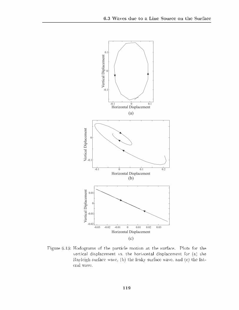
6.3 Waves due to a Line Source on the Surface
-0.1 0 0.1
-0.1
0
0.1
Ver
tica
lD
ipla
cem
ent
Ver
tica
lD
ipla
cem
ent
Ver
tica
lD
ipla
cem
ent
Horizontal Displacement
Horizontal Displacement
Horizontal Displacement
-0.03 -0.02 -0.01 0 0.01 0.02 0.03-0.02
-0.01
0
0.01
-0.1 0 0.1 0.2
-0.1
0
(a)
(b)
(c)
Figure 6.13: Hodograms of the particle motion at the surface. Plots for thevertical displacement vs. the horizontal displacement for (a) theRayleigh surface wave, (b) the leaky surface wave, and (c) the lat-eral wave.
119

CHAPTER 7
Propagation and Scattering of Elastic
Waves in the Ground
In laboratory experiments, inert land mines are buried in a large sand-�lled tank.
Elastic waves are excited, and the displacement of the surface above the mine is
measured using a radar system. To analyze the experimental results, the experiments
are duplicated with the numerical model. In this chapter, results obtained with the
numerical model are presented. The chapter is divided into two main sections. In the
�rst section, the numerical model is used to explore the propagation of elastic waves
along the surface of the ground. In the second section, the interaction of elastic waves
with buried anti-personnel and anti-tank mines is investigated.
For the numerical model, the soil is assumed to be linear, isotropic and lossless.
In that case, the elastic properties of the soil can be completely described by three
independent parameters: the material density, the shear wave speed, and the pres-
sure wave speed. In order to model the soil and its behavior accurately within the
numerical model, these parameters have been measured as a function of depth in the
sand used in the experiments.
The measurements of the material properties and their results are described in
detail in Chapter 9 and shall be summarized only brie y at this point. The wave
speeds in the ground have been estimated by burying a vertical array of accelerome-
ters. By using the accelerometers and displacing the transducer, the arrival times of
120

Propagation and Scattering of Elastic Waves in the Ground
the wave fronts as a function of depth and distance are determined. From the arrival
times, the wave speeds of the various wave types in the ground can be estimated.
The material density, the pressure wave speed and the shear wave speed as a
function of depth are shown in Fig. 7.1. All three quantities have been found to be
depth dependent. The material density has a value of roughly 1430 kg/m3 at the
surface and increases to about 1670 kg/m3 at a depth of half a meter. The variation
in the material density is due to changes in the water content within the soil. At
the surface, the sand is fairly dry. Within the ground, the water content increases
steadily, until the water table is reached at a depth of about half a meter. The pressure
wave speed and the shear wave speed both also vary with depth. At the surface, a
layer with fairly slow wave speeds exists. Beyond this layer, the wave speeds increase
rapidly. At a depth of half a meter, the pressure wave speed and the shear wave
speed have values of 210 m/s and 130 m/s, respectively.1 The material properties of
all other materials used in the following are summarized in Table 7.1. Note that the
shear wave speed in air is zero, and, consequently, shear waves cannot propagate in
air.
Table 7.1: Material properties.
Shear Wave Pressure Wave Material
Speed Speed Density
cS [m/s] cP [m/s] � [kg/m3]
Plastic 1100 2700 1200
Air 0 330 1.3
Rubber 500 800 1000
1The material properties are measured only to a depth of half a meter and are assumed to beconstant deeper in the ground. This is a vague assumption and probably not true within the watertable, but is justi�able, because, within the frequency range of interest, the variation of the materialproperties deeper in the ground will not have a signi�cant impact onto the wave propagation at andclose to the surface.
121

Propagation and Scattering of Elastic Waves in the Ground
1400
1450
1500
1550
1600
1650
1700
1750
Mat
eria
lD
ensi
ty[k
g/m
]3
0 10 20 30 40 50Depth [cm]
0 10 20 30 40 50Depth [cm]
80
100
120
140
160
180
200
220
Wav
eS
pee
d[m
/s]
Pressure Wave Speed
Shear Wave Speed
Figure 7.1: Variation of the material properties with depth.
122

Propagation and Scattering of Elastic Waves in the Ground
In the experiments, the elastic waves are excited by a transducer placed on the
surface of the ground. The transducer foot, which is in contact with the soil, has
the shape of a bar. In the numerical model, the transducer is emulated by exciting
the particle displacement component normal to the surface throughout an area that
approximately equals the shaker foot in size and shape. The motion of the shaker
foot has been measured using accelerometers and has been found to closely resemble a
di�erentiated Gaussian pulse. For all results in this chapter, a di�erentiated Gaussian
pulse with a center frequency of about 450 Hz is used as excitation.
Formally, the particle velocity is excited in the numerical model, and the particle
velocity is computed as a function of time. Due to the linearity of the numerical
model, the velocity �elds due to the excitation of the particle velocity will be equal to
the displacement �elds, if the displacement rather than the velocity is excited. The
model can be viewed as a linear system: the input is the particle velocity excitation,
and the output are the computed particle velocity �elds. If both input and output
are integrated with respect to time, i. e., if transforming both the input and the
output to the particle displacement, the results will not change. In other words, the
particle displacement �elds due to the excitation of the particle displacement with
a di�erentiated Gaussian pulse are equivalent to the particle velocity �elds due to
the excitation of the particle velocity with a di�erentiated Gaussian pulse, because
the displacement is just the time integral of the velocity. In the experiments, the
particle displacement is measured and compared to the particle displacement �elds
as determined with the numerical model.
In the following, results are presented that are obtained with the numerical model
in two and three dimensions. For both, a spacing of 0.5 cm between the nodes of the
�nite-di�erence grid is chosen, which satis�es the 10-nodes-per-wavelength require-
ment as stated in Eq. (4.32) for the frequency range of interest. The time increment
is determined accordingly to satisfy the Courant condition. Because the maximum
time increment according to the Courant condition depends on the maximum wave
speed occurring in the model, di�erent time steps are used for the di�erent studies.
123

7.1 Surface Waves
When modeling a mine, the maximum time increment is �t = 1:309 � 10�6 s for the2-D model and �t = 1:069 � 10�6 s for the 3-D model. To compute the wave �elds
up to 30 ms, roughly 23000 time steps are necessary for the 2-D model and about
28000 for the 3-D model. The computations took about 45 minutes for the 2-D model
(using a grid with 280� 170 cells) on a 400-MHz single-processor PC, and about 92
minutes for the 3-D model (with 294� 50� 70 cells) on a Beowulf computer cluster
containing 28 500-MHz processors connected in parallel.
In this chapter, results obtained with the numerical model will be compared to
experimental measurements. All measurements that are described here have been per-
formed in an indoor laboratory at the Georgia Institute of Technology by W.R. Scott,
G.D. Larson, and J.S. Martin. The measurement procedure is described in more detail
in Chapter 9.
7.1 Surface Waves
Using the numerical model, the propagation of elastic waves in the ground and along
the surface is studied. The simulation space spans a surface area of 1.67 m by 0.8 m
and has a depth of 0.6 m. Two cases are considered: a homogeneous ground and
an inhomogeneous ground. For the homogeneous case, the material properties are
assumed to be constant throughout the ground. For the inhomogeneous case, the
material properties are assumed to exhibit the depth dependence that has been mea-
sured experimentally (see Fig. 7.1).
First, the elastic wave propagation is determined assuming the ground to be
homogeneous. The material density in the ground is set to 1400 kg/m3, and the
pressure wave speed and the shear wave speed are 250 m/s and 87 m/s, respectively.
Fig. 7.2 shows waterfall graphs of the vertical particle displacement at the surface as
measured experimentally and as determined numerically. In these graphs, the vertical
particle displacement at a number of points along a line on the surface is plotted as
a function of time. The time traces are o�set along the vertical axis by the distance
124
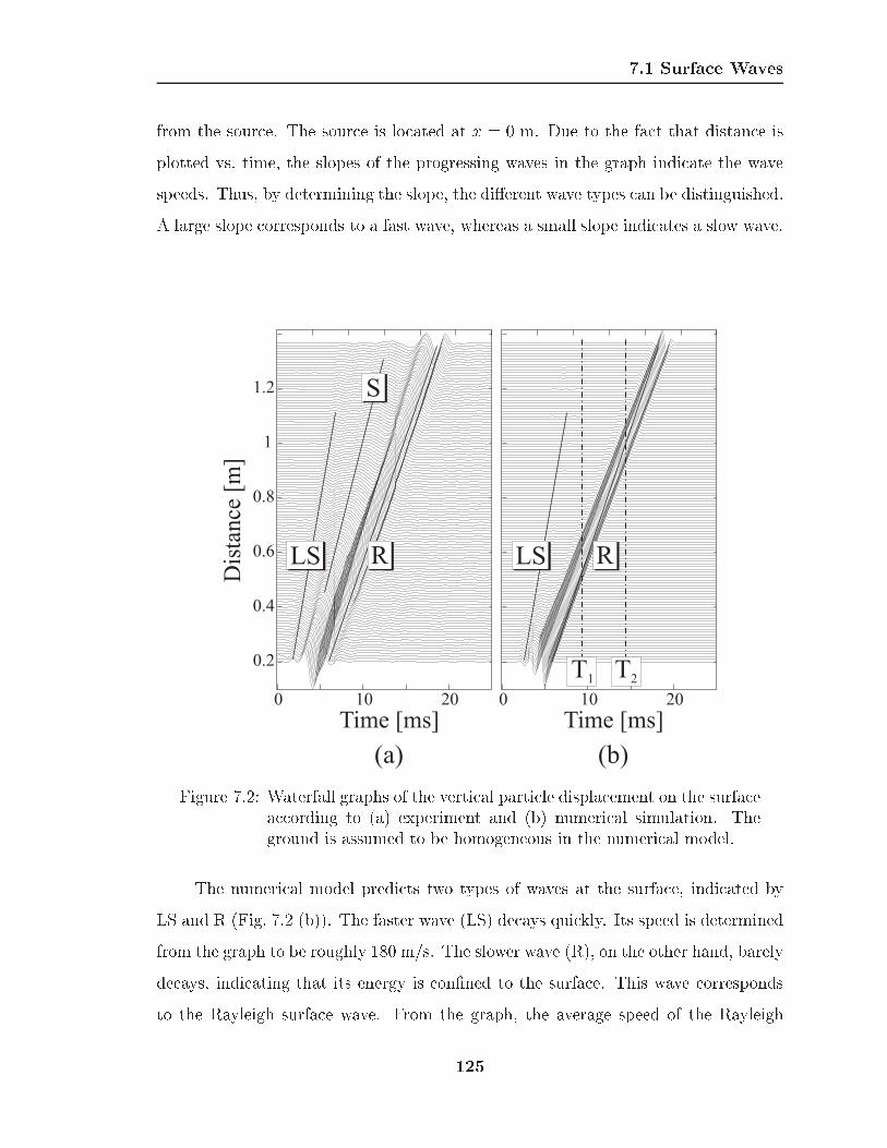
7.1 Surface Waves
from the source. The source is located at x = 0 m. Due to the fact that distance is
plotted vs. time, the slopes of the progressing waves in the graph indicate the wave
speeds. Thus, by determining the slope, the di�erent wave types can be distinguished.
A large slope corresponds to a fast wave, whereas a small slope indicates a slow wave.
(a) (b)
0.2
0.4
0.6
0.8
1
1.2
Dis
tan
ce[m
]
0 010 1020 20
Time [ms] Time [ms]
T1 T2
S
LS R LS R
Figure 7.2: Waterfall graphs of the vertical particle displacement on the surfaceaccording to (a) experiment and (b) numerical simulation. Theground is assumed to be homogeneous in the numerical model.
The numerical model predicts two types of waves at the surface, indicated by
LS and R (Fig. 7.2 (b)). The faster wave (LS) decays quickly. Its speed is determined
from the graph to be roughly 180 m/s. The slower wave (R), on the other hand, barely
decays, indicating that its energy is con�ned to the surface. This wave corresponds
to the Rayleigh surface wave. From the graph, the average speed of the Rayleigh
125

7.1 Surface Waves
wave comes out to be approximately 80 m/s. The experimental result (Fig. 7.2 (a))
looks quite di�erent. A third type of wave is observed, having a wave speed along
the surface larger than the Rayleigh wave, but slower than the fast wave. Also,
the Rayleigh wave in the experiment is seen to be dispersed as it propagates along
the surface, an e�ect that is not predicted by the numerical model if the ground is
assumed to be homogeneous.
To distinguish and explain the waves that are observed on the surface of the
ground, the particle displacement beneath the surface is studied. Fig. 7.3 shows
the vertical particle displacement on the surface and on a cross section through the
ground as computed with the numerical model. Again, the ground is assumed to
be homogeneous. Pseudo-color plots are used to represent the wave �elds, with a
logarithmic scale ranging from red (0 dB) to blue (�50 dB). The wave �elds are
shown at two instants in time, T1 and T2, corresponding to the vertical lines in
Fig. 7.2 (b). The source is located on the surface, to the left of the plot. At T1,
a Rayleigh surface wave (R), a shear wave (S) and a pressure wave (P) are seen to
propagate. On the cross section an additional surface wave (LS) is observed. This
surface wave corresponds to the leaky surface wave that has been discussed in length
in Chapter 6. It travels along the surface with a wave speed faster than the shear
wave, but slower than the pressure wave. Because it is faster than the shear wave, the
leaky surface wave couples into a plane shear wave. Due to these coupling e�ects, the
leaky surface wave decays rapidly in its propagation direction. On the surface plane,
the leaky surface wave is clearly visible, whereas the pressure wave is not recognizable
on the 50-dB scale. This suggests that the fast wave that has been observed in Fig. 7.2
in both experiment and numerical simulation corresponds to the leaky surface wave.
At a later time, at T2, the waves have propagated farther. The leaky surface wave has
mainly decayed, and the pressure wave has left the range of the plot. On the surface
only the Rayleigh wave is visible, whereas on the cross section both the Rayleigh wave
and the shear wave are evident.
In Chapter 6, the elastic waves at and close to the surface have been determined
126

7.1 Surface Waves
R
S
R
R LS
S
R
P
LS
T1
T2
0 dB
-50 dB
Figure 7.3: Normal particle displacement on the surface (top) and on a crosssection through the ground (bottom). The ground is assumed tobe homogeneous. T1 and T2 correspond to the vertical lines inFig. 7.2 (b).
127

7.1 Surface Waves
analytically. It has been found that a leaky surface wave, similar to the one observed
in Fig. 7.3, will be excited by a line source on the surface of the ground. The leaky
surface wave will cause a prograde particle motion on the surface, distinguishing it
from the Rayleigh surface wave, which causes a retrograde motion. To verify this for
the results shown in Fig. 7.3, the particle motion due to the waves on the surface
is analyzed. In Fig. 7.4, the particle displacement is plotted at one point on the
surface (60 cm from the source) as a function of time. Two hodograms are shown
beneath the graph. In these hodograms, the vertical displacement is plotted versus
the horizontal displacement and, thus, the actual particle motion is traced. The
hodogram on the left describes the leaky surface wave, the hodogram on the right
corresponds to the Rayleigh surface wave. As predicted, the leaky surface wave
describes a prograde (clockwise) motion, whereas the Rayleigh surface wave causes a
retrograde (counterclockwise) motion. The prograde particle motion is caused by the
vertical displacement leading the horizontal displacement in phase. The retrograde
motion, on the other hand, is due to the vertical displacement lagging behind in
phase. Note that the pressure wave arrives prior to the leaky wave (see the magni�ed
portion in Fig. 7.4). Both the pressure wave and the leaky wave are much weaker on
the surface than the Rayleigh wave. The particle motion due to the pressure wave is
linear, i. e., the horizontal and vertical component are in phase.
Experimental observations indicate that the Rayleigh wave is dispersed as it
propagates along the surface. This e�ect is believed to be mainly due to the material
properties in the ground varying with depth. The Rayleigh wave decays exponen-
tially into the ground. The rate of decay depends on frequency: high-frequency
components will decay fairly quickly, whereas low-frequency components reach deep
into the ground. If the material properties vary with depth, the di�erent frequency
components will experience di�erent material properties and, thus, di�erent wave
speeds. Consequently, the Rayleigh wave is dispersed.
Fig. 7.5 shows results that are obtained when implementing the depth variation
that has been measured for the soil used in the experiments. Both in the experiment
128

7.1 Surface Waves
0 10 20
Time [ms]
Dis
pla
cem
ent
VerticalHorizontal
LS R
Figure 7.4: Top: particle motion on the surface at a distance of 60 cm fromthe source as a function of time. Bottom: vertical vs. horizontaldisplacement for the leaky surface wave and the Rayleigh surfacewave. Homogeneous case.
129

7.1 Surface Waves
and in the numerical model, three types of waves are observed, indicated by LS, S
and R. The fastest wave of the three, the leaky surface wave (LS), decays quickly.
Its speed is determined to be approximately 180 m/s. The second-fastest wave (S)
has a speed of roughly 120 m/s and is fairly weak at the surface. Its origin cannot
be clearly identi�ed from this graph. The slowest wave is the Rayleigh surface wave
(R) with a wave speed of about 80 m/s. Clearly, the Rayleigh wave is dispersed
as it propagates. The agreement of experiment and numerical simulation is fairly
good. The di�erences in Fig. 7.5 are believed to be mostly due to non-linear e�ects
occurring in the sand. The non-linearities dampen the high-frequency components
and, in this way, cause the pulse to broaden and to change in shape. By decreasing
the amplitude of the excitation in the experiment, the agreement of experiment and
numerical simulation can be improved. However, the signal-to-noise ratio of the radar
output in the experiment will also decrease and, thus, the noise content of the data
will increase.
Fig. 7.6 shows the vertical particle displacement on the surface and on a cross
section through the ground as computed with the numerical model for the inhomo-
geneous ground. The wave �elds are shown at two instants in time, T1 and T2. It
is evident that, by assuming the material properties in the ground to be inhomoge-
neous, the wave �elds within the ground are signi�cantly altered. At T1, the Rayleigh
surface wave (R), the shear wave (S), the pressure wave (P) and the leaky surface
wave (LS) are seen. As suggested by the depth pro�le, the shear wave is faster within
the ground than for the homogeneous case. At a later time, at T2, the leaky surface
wave has decayed. Due to the rapid increase of the shear wave speed beyond the
surface layer, a portion of the shear wave is refracted back towards the surface, and a
guided shear wave arises. It is this guided shear wave that is the second wave evident
at the surface in Fig. 7.5. The guided shear wave is strongly visible at the surface. It
is faster than the Rayleigh surface wave, but slower than the shear wave within the
ground.
In Fig. 7.7, the particle motion due to the waves on the surface is analyzed for
130

7.1 Surface Waves
(a) (b)
0.2
0.4
0.6
0.8
1
1.2
Dis
tan
ce[m
]
0 010 1020 20
Time [ms] Time [ms]
T1 T2
LS R LS R
SS
Figure 7.5: Waterfall graphs of the vertical particle displacement on the surfaceaccording to (a) experiment and (b) numerical simulation. Thematerial properties in the numerical model are assumed to varywith depth.
131

7.1 Surface Waves
R
S
S
R S
SR LS
S
R
P
LS
T1
T2
Figure 7.6: Normal particle displacement on the surface (top) and on a crosssection through the ground (bottom). T1 and T2 correspond to thevertical lines in Fig. 7.5 (b). Depth-varying material properties areassumed.
132

7.2 Interaction of Elastic Waves with Buried Land Mines
the inhomogeneous case. The particle displacement is again plotted at one point on
the surface (60 cm from the source) as a function of time. As for the homogeneous
case, the leaky surface wave causes a prograde particle motion, whereas the Rayleigh
surface wave induces a retrograde motion. The guided shear wave is clearly visible. It
arrives ahead of the Rayleigh wave and has a predominantly vertical particle motion.
7.2 Interaction of Elastic Waves with Buried Land
Mines
The interaction of elastic waves with buried land mines is to be investigated. For
this, the mine-wave interaction is computed with the numerical model both in 2-D
and in 3-D and compared to experimental results.
In the experimental system, the waves are excited from a transducer on the
surface and detected by a radar system mounted above the surface. Fig. 7.8 shows a
schematic drawing of two possible set-ups for such a system. In the �rst set-up, the
waves are excited by a transducer (the Source) and recorded by an array of receivers
placed at some distance from the transducer (top of Fig. 7.8). The array consists of
a number of receivers, which simultaneously record their signal, yielding a fast scan
rate and a small detection time. In another set-up, the array is realized as a synthetic
receiver array. Hence, only one receiver is moved across the surface and records the
signal that is excited repeatedly from the transducer. This second set-up (bottom
of Fig. 7.8) yields a much more cost-e�ective system, but prolongs the scan time
enormously. Currently, the second set-up is implemented in the experimental sensor
system [14, 12]. A radar is used as receiver. The radar scans across the surface and
measures the displacement of the surface as a function of time.
To investigate the interaction of elastic waves with a buried anti-personnel mine,
a very simple model is used to approximate the mine's structure within the numerical
133

7.2 Interaction of Elastic Waves with Buried Land Mines
0 10 20
Time [ms]
Dis
pla
cem
ent
VerticalHorizontal
LS R
S
Figure 7.7: Top: particle motion on the surface at a distance of 60 cm fromthe source as a function of time. Bottom: vertical vs. horizontaldisplacement for the leaky surface wave and the Rayleigh surfacewave. Depth-varying material properties are assumed.
134

7.2 Interaction of Elastic Waves with Buried Land Mines
Source Receiver Array
Source Synthetic Receiver Array
Figure 7.8: Schematic drawing of possible set-ups for the experimental system.
model. Fig. 7.9 shows the simple mine model, together with a simpli�ed cross sectional
drawing and a photograph of a TS-50 anti-personnel mine. The simple mine model
consists of a large plastic chamber, and a small air-�lled chamber. In the cubic �nite-
di�erence grid, the cylindrical shape of the mine is approximated by cubes, leading
to the stair-case form evident in Fig. 7.9. The air-�lled chamber is inserted into the
model to approximate the structure of the TS-50 mine. A real land mine has a fairly
complex structure, containing explosives, a trigger mechanism and several chambers.
7.2.1 2-D Analysis
As a �rst approach, the 2-D model is used to study the interaction of elastic waves
with a buried anti-personnel mine. The model for the mine used in the 2-D model, as
135

7.2 Interaction of Elastic Waves with Buried Land Mines
Air
Explosives Detonator
Firing PinRubber Pressure Plate Spring
Plastic Case
3 cm
Air
Plastic
8 cm
Figure 7.9: Simple model for the TS-50 anti-personnel mine; cross-sectionaldrawing and photograph of a real TS-50 mine.
136

7.2 Interaction of Elastic Waves with Buried Land Mines
shown in Fig. 7.10, is the 2-D projection of the 3-D mine model. The mine is buried
2 cm beneath the surface of the ground, at a distance of 60 cm from the source. A
point source placed on the surface excites the vertical particle displacement using a
di�erentiated Gaussian pulse with a center frequency of 450 Hz. The elastic wave
�elds are computed on a grid containing 280 by 170 cells, including a PML with a
thickness of 10 cells and, consequently, yielding an e�ective solution space of 130 cm
by 80 cm. For the 2-D model, the material properties in the ground are assumed to
be homogeneous: � = 1400 kg/m3, cP = 250 m/s, and cS = 87 m/s.
60 cm
8 cm
4 cm2 cm
Source Mine
Figure 7.10: 2-D model for an anti-personnel mine.
Figure 7.11 shows the elastic wave �elds on a cross section through the ground
as computed with the 2-D model. As earlier, the vertical particle displacement is
plotted using a logarithmic color scale with a dynamic range of 50 dB. The wave
�elds are shown at four di�erent times. At T1, a pressure wave (P), a shear wave (S),
a Rayleigh surface wave (R) and a leaky surface wave (LS) are observed. The pressure
wave, the fastest of the waves, just hits the mine. At T2, the Rayleigh wave (R) has
reached the mine. At T3, the incident waves are seen to be scattered. Cylindrical
wave fronts arise. Scattered Rayleigh waves as well as shear waves are induced. At
T4, the incident waves have passed the mine. However, some energy appears to be
trapped above the mine, and continuous resonant oscillations occur. Due to these
oscillations, waves are radiated from the mine location.
137

7.2 Interaction of Elastic Waves with Buried Land Mines
0 dB -50 dB
T1
S
P
LSR
T2
R
LS
S
T3 T4
Figure 7.11: Interaction of elastic waves with a buried anti-personnel mine; 2-Dresults.
138

7.2 Interaction of Elastic Waves with Buried Land Mines
To explore the origin of the resonance and its nature, the mine is elongated
within the numerical model, as shown in Fig. 7.12. The modi�ed mine model has
a length of 54 cm and an air chamber that is 50 cm long. Fig. 7.13 shows the
54 cm
50 cm
2 cm
3 cm
1 cm
Air
Plastic
Ground
Figure 7.12: Model to determine the nature of the resonance: elongated mine.
vertical particle displacement on the surface in a waterfall graph as obtained with the
modi�ed model. A leaky surface wave (LS) and a Rayleigh wave (R) are seen to be
incident on the mine. Both waves hit the mine and are partially re ected and partially
transmitted. Above the mine, a complex pattern of propagating waves arises. This
can be explained as follows. When the incident waves interact with the mine, they
couple primarily into three di�erent wave portions: into re ected waves (rR), into
waves which are transmitted through the plastic body underneath the air chamber
(M), and into waves which propagate within the thin soil layer between the surface
and the air chamber (L and TF). Because the plastic body lies underneath the air
chamber, the waves transmitted through the plastic are not visible on the surface.
This is evident in Fig. 7.13: a wave arises beyond the mine, apparently without being
caused by any wave visible on the surface above the mine. The path the wave takes
through the plastic is indicated by M. The Rayleigh wave couples a signi�cant amount
of energy into the thin layer above the air chamber. Two di�erent kinds of waves
139

7.2 Interaction of Elastic Waves with Buried Land Mines
arise within the thin layer: a longitudinal wave (L) and a transverse exural wave
(TF). The longitudinal wave is the faster one of the two. It propagates within the
thin layer between surface and air chamber (L), is re ected at the edge of the air
chamber, travels back within the layer and is re ected again. The transverse exural
wave also travels within the layer between surface and air chamber (TF), is re ected,
travels back and is again re ected. Note that the exural waves are almost completely
re ected at the edges of the air chamber, and the energy remains within the thin layer
above the mine. Figure 7.14 explains schematically the paths the various waves follow
through and around the mine.
Using the modi�ed model, the resonant behavior of the mine in the numerical
model can be explained. When the waves interact with the mine, they are partially
re ected and partially transmitted. However, a large portion of the energy couples
into longitudinal and transverse- exural waves in the thin soil layer above the mine.
Due to the small size of the mine, these waves form standing waves, giving rise to the
resonant oscillations observed in Fig. 7.11.
From the slopes of the traveling waves in Fig. 7.13, the wave speeds of the longi-
tudinal wave (L) and the transverse exural wave (TF) are approximately determined
to be cL � 160 m/s and cTF � 50 m/s, respectively. A simple theory for waves propa-
gating in a thin plate with clamped edges predicts the wave speeds of the longitudinal
wave to be [58]
cL =
E
�(1� �2)
!1=2
; (7.1)
and the wave speed of the transverse exural wave to be
cTF =
vuuth!
E
12�(1� �2)
!1=2
; (7.2)
where E and � are Young's modulus and Poisson's ratio (see Appendix D); � is the
material density, and h is the thickness of the thin plate. For the longitudinal wave,
this yields a wave velocity of cL = 163 m/s. For the transverse exural wave with
a center frequency fc = 450 Hz and a plate thickness of h = 2 cm, a wave speed of
140

7.2 Interaction of Elastic Waves with Buried Land Mines
0
0.2
0.4
0.6
0.8
1
1.2
Dis
tance
[m]
5 10 15 20 25
Time [ms]
LL
rRR
TFTF
LS
MMMM
LS
R
L
M
TF
rR
Pressure Wave
Rayleigh Wave
Longitudinal Wave
Transverse FlexuralWave
Wave through Mine
Reflected RayleighWave
Figure 7.13: Flexural waves propagating above the mine.
rR L, TF RR, LS
M
Figure 7.14: Wave paths through and around the mine. The incident Rayleighwave (R) and leaky surface wave (LS) couple into a longitudinalwave (L) and a transverse exural wave (TF) in the thin plateabove the mine and into a wave passing through the plastic bodyof the mine (M).
141

7.2 Interaction of Elastic Waves with Buried Land Mines
cTF = 52 m/s is predicted. This is in good agreement with the wave speeds obtained
from the numerical simulation. Note that the wave speed of the transverse exural
wave is dependent on frequency, while the speed of the longitudinal wave is not. Thus,
the transverse wave is strongly dispersive. The dispersion of the transverse exural
wave can be clearly seen in Fig. 7.13.
7.2.2 3-D Analysis
The experimental model is inherently three-dimensional, and, thus, a 3-D model is
needed to adequately simulate the experiments. Using the 3-D model, the interaction
of elastic waves with buried mines is investigated as a function of burial depth, and
the results obtained with the numerical model are compared to experimental results.
Anti-Personnel Mine
With the 3-D model, the wave �elds are computed throughout a solution space with
a surface area of 1.67 m by 0.8 m and a depth of 0.4 m. The mine model as shown in
Fig. 7.9 is used, and the numerical results are compared to experimental results. Both
in experiments and numerical simulations, the mine is placed at a distance of 97 cm
from the source. The material properties are assumed to vary with depth according
to Fig. 7.1.
Fig. 7.15 shows pseudo-color plots of the vertical particle displacement on the
surface plane (top) and on a cross section through the ground (bottom). The color
scale ranges from red (0 dB) to blue (-50 dB). The wave �elds are shown at four
instants in time. The mine is placed 2 cm beneath the surface. At T1, the guided
shear wave (S) just hits the mine. On the cross section, the shear wave (S) and the
Rayleigh wave (R) are seen. The leaky surface wave is faintly visible on the surface
plane (LS). The pressure wave has already left the range of the plot. At T2, the
Rayleigh wave has reached the mine. Scattered cylindrical wave fronts appear at the
surface, which are re ections from the incident guided shear wave. At T3, scattered
142

7.2 Interaction of Elastic Waves with Buried Land Mines
S
SR
rR
T2
R
rR
T3
R
rR
T4
S LSR
SR
T1
Figure 7.15: Interaction of elastic waves with a buried anti-personnel mine;pseudo color plots of the normal particle displacement on the sur-face (top) and on a cross section through the ground (bottom) atfour instants in time.
143

7.2 Interaction of Elastic Waves with Buried Land Mines
waves from both the guided shear wave and the Rayleigh wave are visible. The leading
wave fronts are re ections from the incident guided shear wave. The strong waves
that follow are due to the Rayleigh wave. At T4, resonant oscillations are visible at
the location of the buried mine. In cylindrical wave fronts, energy is radiated out.
As observed with the 2-D model, the resonant oscillations are con�ned to the thin
soil layer above the mine. Due to these oscillations, the mine location can be clearly
identi�ed on the surface.
To compare numerical to experimental results, the vertical surface displacement
is plotted in a set of waterfall graphs. Fig. 7.16 shows these waterfall graphs for (a)
experimental and (b) numerical results. Mines at four di�erent depths are considered,
at 1 cm, 2 cm, 3 cm, and 6 cm (from left to right). The mine, indicated by the gray
shading, is located at a distance of 97 cm from the source. For the mine at 1 cm, strong
oscillations are visible at the mine location. In the experiment, the amplitude of the
oscillations appears larger, but the oscillations decay faster than in the numerical
simulation. For the mines at 2 and 3 cm, the oscillations are weaker, but still clearly
visible. For the mine at 6 cm, the oscillations are very weak and cannot be seen in
this graph. However, by applying signal processing techniques the e�ects of the mine
can be enhanced, making it easier to locate the buried mine [12].
The agreement between the numerical and experimental results is surprisingly
good considering the uncertainties of the material parameters for the ground in the
experimental model and the simpli�cations made in the numerical model. For the
numerical model, it has been shown with the 2-D model that the oscillations at the
mine location are caused by the incident waves coupling into exural waves in the
thin soil layer above the mine. These exural waves are con�ned to the thin layer
and form a standing wave pattern, giving rise to the resonant oscillations. As the
burial depth of the mine is increased, the soil layer becomes thicker, causing the
exural waves to be dampened, because more energy is radiated out. The resonance
in the experimental results has a more complex shape. In the experimental model,
the resonance is strongly in uenced by the resonant behavior of the actual buried
144

7.2 Interaction of Elastic Waves with Buried Land Mines
Time [ms]
0.4
0.6
0.8
1.0
1.2
1.4
1.6
Dis
tan
ce[m
]
15 3015 3015 300 15 30
(a)
Time [ms]
0.4
0.6
0.8
1.0
1.2
1.4
1.6
Dis
tan
ce[m
]
15 3015 3015 300 15 30
(b)
Figure 7.16: (a) Experimental results for a buried TS-50 anti-personnel mineand (b) numerical results for a simple anti-personnel mine model;waterfall graphs of the vertical particle displacement on the surface.Land mine buried at 1 cm, 2 cm, 3 cm, and 6 cm (from left to right).
145

7.2 Interaction of Elastic Waves with Buried Land Mines
mine. A TS-50 mine has several chambers, it has a exible case that can support
both exural and longitudinal waves, and it contains springs that can also give rise to
resonances. Furthermore, the soil above the mine might act in a strongly non-linear
way, thus altering the shape of the resonance.
To compare the interaction of the elastic waves with a buried mine to, for ex-
ample, the interaction with a buried rock, a solid body is inserted into the numerical
model. The body has a spherical shape and a diameter of 8 cm. Its properties are
assumed to be the same as the ones of plastic (see Table 7.1). The results are shown
in Fig. 7.17 in some pseudo-color plots for the sphere buried 2 cm beneath the surface
and in Fig. 7.18 in some waterfall graphs for the sphere at di�erent depths. When
the incident waves interact with the solid sphere, re ections occur which have about
the same strength and shape as the re ections that have been observed for the buried
anti-personnel mine. However, no continuous oscillations are visible at the location
of the sphere, thus clearly distinguishing the solid body from the buried mine. Very
similar results have also been observed experimentally.
Anti-Tank Mine
Next, the interaction of elastic waves with an anti-tank mine is to be analyzed.
Fig. 7.19 shows a simple model for an anti-tank mine and a photograph of a VS
1.6 mine. The mine has a diameter of about 23 cm and, thus, is substantially larger
than the anti-personnel mine. The simple mine model contains three parts: a large
plastic body, an air-�lled chamber, and a rubber plate simulating the pressure plate
of the mine.
In Fig. 7.20, the interaction of elastic waves with an anti-tank mine is shown in
some pseudo-color plots. The mine is buried 4 cm beneath the surface, and its center
is placed at a distance of 77 cm from the source. As before, a logarithmic color scale
with a dynamic range of 50 dB is used. As for the anti-personnel mine, the incident
waves are seen to be scattered by the anti-tank mine. Upon incidence onto the mine,
the waves are partially transmitted and partially re ected. The incident guided shear
146

7.2 Interaction of Elastic Waves with Buried Land Mines
S
SR
rR
T2
R
rR
T3
R
rR
T4
S LSR
SR
T1
Figure 7.17: Interaction of elastic waves with a buried spherical object; pseudocolor plots of the normal particle displacement on the surface (top)and on a cross section through the ground (bottom) at four instantsin time.
147

7.2 Interaction of Elastic Waves with Buried Land Mines
Time [ms]
0.4
0.6
0.8
1.0
1.2
1.4
1.6
Dis
tan
ce[m
]
15 3015 3015 300 15 30
Figure 7.18: Numerical results for a buried sphere; waterfall graphs of the ver-tical particle displacement on the surface. Sphere buried at 1 cm,2 cm, 3 cm, and 6 cm (from left to right).
23 cm
8 cm
Air
Plastic
Rubber
Figure 7.19: Simple model for the VS 1.6 anti-tank mine; schematic picture ofthe model and photograph of a VS 1.6 mine.
148
7.2 Interaction of Elastic Waves with Buried Land Mines
wave (at T1) and the Rayleigh surface wave (at T2) couple into the thin soil layer
above the mine. The pattern of waves that arises above the mine and the shape of
the radiated wave fronts are fairly complex. The waves above the mine, rather than
forming standing waves, propagate in the thin layer and radiate energy as they travel
back and forth across the layer.
Fig. 7.21 shows waterfall graphs according to experimental measurements and
numerical simulations. The location of the mine is indicated by the gray shading.
The mines are buried at four depths: at 2 cm, 4 cm, 6 cm and 10 cm (from left
to right). For the mine at 2 cm and 4 cm, the interaction with the elastic waves is
strong. At the mine location, a complex pattern of waves traveling back and forth
above the mine is visible. This can be explained by using the argument given before
to interpret the oscillations observed for an anti-personnel mine. The incident wave
partially couples into exural waves in the thin soil layer above the mine. For the
anti-personnel mine, these exural waves formed a standing wave pattern. For the
larger anti-tank mine, however, the exural waves propagate in the thin layer, are
re ected at the edge of the mine, propagate back, are again re ected at the other edge
of the mine, and so forth. Due to the large size of the anti-tank mine, the waves do
not form standing waves, but are propagating back and forth. For the anti-tank mine
at 2 cm, the exural waves are almost completely re ected at the edges of the mine
and are con�ned to the soil layer. For the mine at 4 cm, more energy leaks out of the
thin layer and is radiated away. And for the mine at 6 cm, the waves are re ected
only very weakly at the mine's edges. For the mine at 10 cm, barely any interaction
of the incident waves with the buried mine is visible. The results of experimental
measurements and numerical simulations are in fairly good agreement. The waves
above the mine in the numerical results seem to travel faster than in the experimental
results. This may be due to the depth pro�le of the shear wave speed being especially
inaccurate close to the surface, and to the sand behaving in a strongly non-linear
way at the surface. However, in spite of all uncertainties in the characterization of
the soil and the simplicity of the mine model, the same qualitative behavior for the
149

7.2 Interaction of Elastic Waves with Buried Land Mines
S
SR
rR
T2
R
rR
T3
R
rR
T4
S LSR
SR
T1
Figure 7.20: Interaction of elastic waves with a buried anti-tank mine; pseudocolor plots of the normal particle displacement on the surface (top)and on a cross section through the ground (bottom) at four instantsin time.
150

7.3 Mines in the Presence of Clutter
interaction of the elastic waves with the buried mine is observed in experiment and
numerical model.
7.3 Mines in the Presence of Clutter
One of the most crucial requirements for a land mine detection system is the capability
to accurately di�erentiate buried mines from surrounding clutter objects. In the
last section it has been shown that resonant oscillations occur at the location of
a buried mine, when the mine interacts with elastic waves. These resonant e�ects
can be used to enhance the mine's signature, because the resonance appears to be
inherent to minelike objects. It has also been shown that buried rocks will not exhibit
such resonant oscillations. However, the scattering e�ects from buried rocks are
comparable to those from buried mines, and the presence of rocks might signi�cantly
alter the response from the buried mines.
To explore the behavior of mines in the presence of clutter, the interaction of
elastic waves with various mines being surrounded by rocks is computed. Fig. 7.22
shows schematically the con�guration of mines and rocks in the ground and indicates
their sizes and burial depths. The circles indicate the mines, the rectangles mark the
rocks. Four anti-personnel mines are modeled surrounding an anti-tank mine. The
mine closest to the source has a diameter of 6 cm and represents a small anti-personnel
mine. Its distance to the source is 72 cm. The other three anti-personnel mine have
a diameter of 8 cm and lie at distances of 92 cm and 112 cm from the source. The
anti-tank mine, at the center of the scenario, has a diameter of 23 cm. The rocks,
surrounding the mines, are cuboids with dimensions of 6 cm by 8 cm by 4 cm and lie
at di�erent tilt angles with respect to the source. Note that the rock in the lower left
corner is tilted by 30Æ with respect to the surface plane.
Fig. 7.23 illustrates the interaction of the elastic waves with the buried mines
and the rocks. In pseudo-color plots, the vertical particle displacement on the surface
plane is plotted at four times. The source lies to the left of the plots. At T1, the
151

7.3 Mines in the Presence of Clutter
0.3
0.5
0.7
0.9
1.1
1.3
1.5
0 15 30 15 3015 3015 30
Time [ms]
Dis
tance
[m]
(a)
0.3
0.5
0.7
0.9
1.1
1.3
1.5
0 15 30 15 3015 3015 30
Time [ms]
Dis
tance
[m]
(b)
Figure 7.21: (a) Experimental results for a buried VS 1.6 anti-tank mine and(b) numerical results for a simple anti-tank mine model; waterfallgraphs of the vertical particle displacement on the surface. Landmine buried at 2 cm, 4 cm, 6 cm, and 10 cm (from left to right).
152

7.3 Mines in the Presence of Clutter
72 cm
92 cm
112 cm
6 cm
8 cm8cm
8 cm
8 cm
23 cm
1 cm
1 cm
2 cm
2 cm
2 cm
2 cm
4.5 cm
3.5 cm1.5 cm
20
cm20
cm
30
Figure 7.22: Con�guration of the mines and rocks in the ground; the rectan-gles indicate the rocks, the circles indicate the mines. The boxednumbers correspond to the burial depths.
guided shear wave interacts with the mine and the two rocks closest to the source and
is scattered. The leaky surface wave, although weak, has already reached the mine at
the far right. At T2, the Rayleigh surface wave has arrived at the mine closest to the
source. The guided shear wave has passed the anti-tank mine and is seen to strongly
interact with all mines. At T3, the Rayleigh wave has reached the mine farthest from
the source. Resonant oscillations are excited at all mines. At T4, the incident waves
have passed the mine formation. Due to the resonant oscillations, the anti-personnel
mines are clearly discernible on the surface. The interaction of the waves with the
buried mines strongly dominates over the interaction with the clutter. The locations
of the mines can be easily identi�ed, whereas the clutter objects are not apparent on
the surface.
The anti-personnel mines can easily be distinguished from their surroundings,
because resonant oscillations occur at the locations of the buried mines, visible as
bright spots on the surface. From Fig. 7.23, however, the location of the anti-tank
mine cannot be easily identi�ed. Obviously, the interaction of the incident waves with
153

7.3 Mines in the Presence of Clutter
SR
rR
T2
R
rR
T3 T4
T1
R
rR
S LSR
Figure 7.23: Interaction of elastic waves with four anti-personnel mines, one anti-tank mine and four rocks buried in the ground; pseudo color plotsof the normal particle displacement on the surface at four instantsin time.
154

7.4 A Moving-Source/Moving-Receiver System
the anti-tank mine is strong. But, as explained earlier, due to the substantially larger
size of the anti-tank mine compared to the anti-personnel mines, no resonant oscilla-
tions occur at the mine location, but rather a pattern of exural waves propagating
back and forth above the mine. To facilitate the localization of the buried mines,
an imaging algorithm has been developed by A. Behboodian et al. which forms an
image by, in simple words, summing the energy of the back-scattered waves at each
spatial position [77]. Fig. 7.24 shows the image that results when the algorithm is
applied to the numerically computed data and compares it to experimental results
for a similar set-up [78]. A dynamic range of 30 dB is used. For the experimental
results, an M-14, a TS-50, a VS-50 and a PFM-1 anti-personnel mine were buried
around a VS 1.6 anti-tank mine. In the image formed from the numerical data, the
locations of the �ve mines are accurately predicted. The response of three of the �ve
mines in the numerical data, however, is weaker than in the experimental data. For
the anti-tank mine, the image shows the strongest response in both numerical and
experimental data at the back-end of the mine. This is due to the re ections of the
incident waves being strongest at the back of the mine, an e�ect that has also been
observed earlier in Fig. 7.21.
7.4 A Moving-Source/Moving-Receiver System
In the previous sections, a detection system has been investigated in which the source
was at rest and either a stationary receiving array or a synthetic array with a moving
receiver was used. Ultimately, this system will be mobile, scanning step by step
across the potential mine �eld. For a mobile sensor, other con�gurations, however,
are possible. Fig. 7.25 shows schematically a mine detection system in which both
the source and the receiver are moving. In this system, a constant distance between
source and receiver is maintained, while the source-receiver unit scans across the
surface of the ground.
To investigate such a moving-source/moving-receiver system, the system is sim-
155

7.4 A Moving-Source/Moving-Receiver System
(a)
(b)
Figure 7.24: Image formed from the interaction of elastic waves with the buriedmines using an imaging algorithm; (a) numerical data, (b) exper-imental data. The image describes a surface area of 120 cm by80 cm.
156

7.4 A Moving-Source/Moving-Receiver System
Source Receiver
Figure 7.25: Schematic drawing of the moving-source/moving-receiver system.
ulated with the numerical model. For this, a point source is placed on the surface and
excites elastic waves. The normal particle displacement is excited using a di�erenti-
ated Gaussian pulse with a center frequency of 450 Hz. At some distance from the
source, the vertical particle displacement is recorded at one point, i. e., at the receiver
location, as a function of time. Then, the source is moved by an incremental distance,
and so is the receiver location. Each time trace is plotted and vertically displaced
by the receiver location relative to the buried land mine. A waterfall graph arises, in
which the vertical displacement is plotted as a function of time for all source/receiver
positions.
Fig. 7.26 shows waterfall graphs for a moving-source/moving-receiver system
with di�erent distances between the source point and the receiver location. The
distances between source and receiver are 0 cm, 10 cm, 20 cm, and 30 cm (from left to
right). In the graphs, the time traces of the received signal are vertically displaced by
the distance from the receiver to the center of the mine. Thus, a value of 0 cm on the
vertical axis indicates that the receiver is directly above mine. Two sets of waterfall
graphs are shown: in the �rst the results are scaled so that the maximum peak value
of the �rst time trace is equal in all graphs, whereas in the second the results are not
scaled. In the second set, the peaks for the 0 cm and 10 cm cases are clipped, because
the maximum would otherwise exceed the range of the plot. Each waterfall graph
exhibits three di�erent kinds of waves, corresponding to di�erent signal paths from
the source to the receiver. One path is the direct path (D) and corresponds to the
elastic waves that are excited by the source and propagate directly to the receiver.
157

7.4 A Moving-Source/Moving-Receiver System
In general, this is the strongest signal picked up by the receiver. The direct path is
a straight line in the waterfall graphs, because the distance from source to receiver
is constant and, thus, the propagation time from source to receiver is independent
of the receiver location. Another path is the re ected path (R). The incident waves
propagate towards the buried mine, are re ected by the mine and are then recorded
by the receiver. Because the receiver detects the surface motion, the re ected waves
will primarily be Rayleigh surface waves. The re ected signal describes diagonal lines
in the waterfall graphs, because, dependent on the receiver location with respect to
the mine, the time the signal takes to travel between mine and receiver varies. The
signal that is received via the re ected path contains the re ection from the mine as
well as the waves that are radiated due to resonant oscillations excited at the mine
location. From the slope of the re ected signal in Fig. 7.26, the wave speed of the
re ected waves is determined to be approximately 80 m/s, and, thus, agrees with
the Rayleigh wave speed. When the receiver location or the source location coincide
with the position of the buried mine, strong resonant oscillations are recorded by the
receiver. If the receiver is at the mine location, it will pick up the oscillations excited
at the mine and thus will receive a strong signal, stronger than any re ections or
radiated waves that the receiver records apart from the mine. If the source is at the
mine location, it primarily will excite the resonant oscillations at the mine, yielding
an enhanced resonance. Due to the enhanced resonance, the radiation from the mine
will be increased, which again leads to a strong signal that is recorded at the receiver
location. As visible in Fig. 7.26, the system is reciprocal: the location of source
and receiver are interchangeable, and it does not matter, whether the source or the
receiver are located at the mine location. The received signal will in both cases be
the same. If the distance between source and receiver is zero (left in Fig. 7.26), strong
resonant oscillations are visible at the mine location. If the distance between source
and receiver is increased, the resonant oscillations appear at two distinct receiver
locations: once when the receiver is above the mine, and once when the source is
above the mine. The re ected signal is not visible in between these two resonant
158

7.4 A Moving-Source/Moving-Receiver System
signals. When the results are scaled according to their maximum (as in (a)), the
re ected waves disappear if the source-receiver distance is zero. This is due to the
enhanced resonance picked up by the receiver at the mine location. If the results
are not scaled, it is evident that the re ected waves in each case have the same
strength. Note that, due to the depth variation in the ground, the pulse disperses as
it propagates along the surface, and thus the received pulse changes in shape as the
distance from the source to the receiver is increased.
Fig. 7.27 explains schematically the paths the signal takes. If source and receiver
are both on the same side of the mine (as in 1 and 3), the receiver will pick up the
signal via the direct path (D) and via the re ected path (R). If source and receiver
are on opposite sides of the mine (as in 2), the receiver will record the direct path, but
the signal induced by the re ections and the radiation from the mine will be weak.
This is clearly visible in Fig. 7.26.
159

7.4 A Moving-Source/Moving-Receiver System
0 10 20 10 20 10 20 10 20
-60
-20
-40
0
20
40
60
Time [ms]
Rec
eiv
erL
oca
tio
n(
[cm
]re
lati
ve
tom
ine) RD D R RD RD
(a)
0 10 20 10 20 10 20 10 20
-60
-20
-40
0
20
40
60
Time [ms]
Rec
eiv
erL
oca
tio
n(
[cm
]re
lati
ve
tom
ine) RD D R RD RD
(b)
Figure 7.26: Moving-source/moving-receiver system; water fall graphs of the ver-tical particle displacement at the receiver location; for four dis-tances between source and receiver: 0 cm, 10 cm, 20 cm, 30 cm(from left to right). (a) Scaled to the maximum value of each graph;(b) not scaled. The peaks in (b) are clipped for the 0 cm- and the10 cm-case.
160

7.4 A Moving-Source/Moving-Receiver System
Source Receiver1
Source Receiver2
Source Receiver3
R
R
D
D
D
Figure 7.27: Signal paths for three positions of the source-receiver system.
161
CHAPTER 8
Modeling of Resonant Structures: the
Resonance Behavior of a Buried Land
Mine
In experimental and numerical studies, resonant oscillations have been observed at
the location of a buried land mine, when the mine is excited by elastic waves. These
resonant e�ects have occurred for mines of di�erent types, shapes and sizes, including
anti-personnel and anti-tank mines. The resonance signi�cantly enhances the signa-
ture of a buried mine and clearly distinguishes it from surrounding clutter objects.
In the previous chapter, a very simple model has been used to compute the inter-
action of elastic waves with a buried anti-personnel mine on a large scale. Although
the mine model is very simple, it predicts resonant oscillations at the location of the
buried land mine that are qualitatively very similar to the oscillations observed in
the experiments. It has been shown that the resonant oscillations in the numerical
model are due to exural waves being trapped in the thin soil layer above the mine.
While this explains the resonance for the numerical model, it gives only one possible
cause for the resonance of an actual mine. An actual mine contains explosives, various
air chambers, a triggering mechanism, and a exible case. All these components of
the mine might have a signi�cant impact on the mine-wave interaction. Therefore,
to investigate the resonant behavior in more detail, a re�ned mine model must be
developed that more closely approximates the structure of an actual mine.
162

8.1 Discretization of Elastic Objects
This chapter is divided into two sections. In the �rst section, the results of a
preliminary study are presented. In this study, the necessary spatial discretization is
determined that is required to simulate the resonant behavior of mechanical structures
accurately with the numerical model. In the second section, a re�ned mine model is
introduced to study the resonance at the location of a buried mine as a function of
burial depth and material properties.
8.1 Discretization of Elastic Objects
A re�ned mine model will have to incorporate the details of the mine. Thus, the new
model will require a much �ner discretization than used previously in the numerical
model. To investigate how �ne the structural details of the mine must be discretized to
model their elastic behavior accurately, the resonant frequencies of various mechanical
objects are computed as a function of the spatial discretization in the numerical model.
Results are presented for a long thin bar, a thin circular plate and a tuning fork.
8.1.1 Long Thin Bar
The long thin bar is shown in Fig. 8.1 as discretized within the numerical model. It
has a length of 20 cm and a cross section of 1 cm by 1 cm. Its material properties are
assumed to be those of plastic: � = 1200 kg/m3, cP = 2700 m/s, and cS = 1100 m/s.
In Fig. 8.1, a grid spacing of 0.5 cm is assumed, yielding a discretization of 2 cells
across the width of the bar. Using the numerical model, the resonant frequencies of
the bar in air are determined in the range up to 1.5 kHz and are compared to results
from a simple analytical theory.
The resonant frequencies for the exural modes of a long thin bar can be calcu-
lated analytically using the simple Bernoulli-Euler theory for long thin rods [58, 79].
The Bernoulli-Euler theory is an approximate theory, because it neglects the e�ects
of shear deformations and the rotary inertia of the bar. It will predict the resonant
163

8.1 Discretization of Elastic Objects
1 cm
20 cm
Figure 8.1: Long thin bar.
frequencies accurately only for the low-frequency harmonics, i. e., if the harmonic
wave length is much larger compared to the width of the bar. For higher harmonics,
the Bernoulli-Euler theory will signi�cantly overestimate the resonant frequencies.
For a bar with free ends, the Bernoulli-Euler theory predicts the resonant fre-
quency of the i-th harmonic to be [79]
fi =K
2�l2
sE
�(�il)
2; (8.1)
where K is the radius of gyration (equal to the height of the bar divided byp12 for
a bar with a rectangular cross section), l is the length of the bar, and E is Young's
Modulus (see Appendix D). The transverse wave number �i is the solution to a
transcendental equation and is given in Table 8.1 for the �rst two harmonics.
Table 8.1: Wave numbers and wave length of the �rst two harmonics of a barwith free ends according to the Bernoulli-Euler theory.
Harmonic Wave Number Wavelength�i � = 2�
�i
1 4:730=l 1:330l
2 7:853=l 0:800l
Using Eq. (8.1), the �rst and second harmonic of the bar are estimated to have
resonant frequencies of 473 Hz and 1303 Hz, respectively. The resonant frequencies as
164

8.1 Discretization of Elastic Objects
computed with the numerical model are summarized in Table 8.2. With the numerical
model, the resonant frequencies are computed as a function of the discretization, i. e.,
for a varying spacing between the nodes in the numerical grid. In Fig. 8.2, the
resonant frequencies and the error relative to the theoretical prediction are plotted
as a function of the number of nodes that are placed across the bar. With two nodes
across the bar, the numerical model predicts resonant frequencies of 405 Hz and 1100
Hz for the �rst two modes, corresponding to an error of about 15 %. With four nodes,
the error has reduced to about 5 %, and for ten nodes it is about 3 %. The relative
error for the second harmonic always exceeds the error for the �rst harmonic. This
is due to the simple analytical theory overestimating the resonant frequency of the
second harmonic. In general, the true error of the numerical results will be smaller
than predicted here, because the actual resonant frequencies will be slightly smaller
than the theoretical predictions.
Table 8.2: Resonant frequencies of a long thin bar.
# nodes across bar 1st Mode [Hz] 2nd Mode [Hz]
2 405 1100
3 430 1170
4 455 1230
5 460 1245
6 460 1255
8 465 1260
10 465 1265
Theoretical 473 1303
165

8.1 Discretization of Elastic Objects
1 2 3 4 5 6 7 8 9 10 11
# Nodes across
FUNDAMENTAL
1. HARMONIC
200
400
600
800
1000
1200
1400
Fre
qu
ency
[Hz]
20
16
12
8
4
0
FUNDAMENTAL
1. HARMONIC
Err
or
[%]
1 2 3 4 5 6 7 8 9 10 11
# Nodes across
(a)
(b)
Figure 8.2: (a) Resonant frequencies of the bar and (b) error relative to thetheoretical prediction as a function of the number of nodes acrossthe width of the bar.
166

8.1 Discretization of Elastic Objects
8.1.2 Thin Circular Plate
Next, a thin circular plate is considered. The plate is shown in Fig. 8.3. It has a
diameter of 20 cm and a thickness of 1 cm. As before, the material properties of
plastic are assumed for the plate. The plate is placed in air and is free along its edge.
20 cm
1 cm
Figure 8.3: Thin circular plate.
The shape of the �rst three modes of a circular plate with a free edge is schemati-
cally shown in Fig. 8.4. The modes are labeled by the number of their nodal diameters
and their nodal circles. For example, the (20)-mode describes a mode with two nodal
diameters and zero nodal circles. Along a nodal diameter or a nodal circle, the dis-
placement of the plate is zero. The fundamental mode of a thin circular plate that
is free along its edge is the (20)-mode, the next higher mode in frequency is the
(01)-mode, followed by the (30)-mode.
Using an approximate theory, the resonant frequencies of a thin circular plate
can be obtained as solutions to a rather complicated transcendental equation [58].
The analytically determined resonant frequencies of the �rst three modes of the thin
circular plate are summarized in Table 8.3 in terms of the frequency of the funda-
mental (20)-mode.
The resonant frequencies of the �rst three modes as computed with the numerical
model are summarized in Table 8.4. Results are listed for three discretizations, namely
167

8.1 Discretization of Elastic Objects
01-Mode
20-Mode
30-Mode
Figure 8.4: Modes of a circular plate with free edge. The bold lines indicatethe nodal diameters and nodal circles.
168

8.1 Discretization of Elastic Objects
Table 8.3: Resonant frequencies of the �rst three modes of a thin circular discthat is free along its edge.
Mode Resonant Frequency[Hz]
(20) f(20) = 0:2413cLh=a2
(01) f(01) = 1:73f(20)
(30) f(30) = 2:33f(20)
where cL =pE=(�(1� �2)) is the
longitudinal wave speed in an in�niteplate, h is the thickness of the plate,and a is its radius.
for two, four and eight cells across the thickness of the plate. The error relative to the
theoretical values is given in brackets. For all three modes, the theoretical predictions
are larger than the numerical values. The relative error reduces as the number of nodes
across the plate is increased, from about 20 % for two nodes to below 10 % for eight
nodes. Again, the simple theory overestimates the resonant frequencies, and, thus,
the actual error of the numerical results will be smaller than stated here.
Table 8.4: Resonant frequencies of the thin circular plate as computed withthe numerical model.
# nodes across plate f(20) [Hz] f(01) [Hz] f(30) [Hz]
2 380 (21%) 715 (15%) 870 (23%)
4 440 (9%) 805 (4%) 1000 (11%)
8 455 (6%) 825 (1.5%) 1030 (9%)
Theoretical 484 839 1129
For both the bar and the plate it is apparent that, in general, the accuracy
of the numerical model will be improved, if the spacing between the nodes of the
169

8.1 Discretization of Elastic Objects
numerical grid is decreased. Considering the high uncertainty in, for example, the
material parameters in the numerical model, one can conclude from the above results
that the resonant behavior of an object will be modeled with a reasonable accuracy,
if four cells are placed across its smallest structural width. Even a discretization with
only two or three cells might suÆce, if a slightly increased error is acceptable in the
numerical model.
8.1.3 Tuning Fork
As a more complex mechanical structure, the resonant behavior of a tuning fork is
explored. The tuning fork, as discretized in the numerical model, is shown in Fig. 8.5.
Its measures are identical to an actual tuning fork with a fundamental frequency of
329.6 Hz, corresponding to the musical tone E. The tuning fork is made out of steel,
approximately described by � = 4100 kg/m3, cP = 5000 m/s, and cS = 3500 m/s.
With the numerical model, the resonant frequencies of the fork in the range up to
1.5 kHz are determined.
1.35 cm
8.8 cm
0.45 cm
2.6 cm
13.2 cm
Figure 8.5: Tuning fork.
The modes of a tuning fork can be classi�ed into four groups: symmetrical
170

8.1 Discretization of Elastic Objects
modes in the plane of the fork's arms (caused by the symmetric motion of the two
arms), antisymmetrical modes in the plane, symmetrical modes normal to the plane
and antisymmetrical modes normal to the plane [80]. In the range up to 1.5 kHz, the
tuning fork will have four modes, one of each of the four groups. The four di�erent
modes are schematically shown in Fig. 8.6. The fundamental mode is the symmetric
in-plane mode.
In-Plane
Symmetric
Antisymmetric
Out-of-Plane
Figure 8.6: Schematic drawing of the �rst four modes of a tuning fork.
Using an approximate theory, the resonant frequencies of the four modes can be
estimated [79, 80]. For the symmetrical in-plane and out-of-plane modes, the motion
of the tines of the tuning fork resembles that of a cantilever beam, clamped at the
forking point. For a cantilever beam with dimensions similar to the arms of the fork
in Fig. 8.5, the resonant frequency is predicted to be approximately 363 Hz. For
the antisymmetrical modes, the entire fork bends in the manner of a beam with free
ends. A beam with a uniform cross section equivalent to the cross section of one arm
of the tuning fork has a resonant frequency of about 1051 Hz. Of course, the fork
does not have a uniform cross section along its length, and, thus, this value is only
a very crude estimate for the resonant frequency of the antisymmtrical modes of the
tuning fork. It must be noted that this theory does not distinguish between in-plane
171
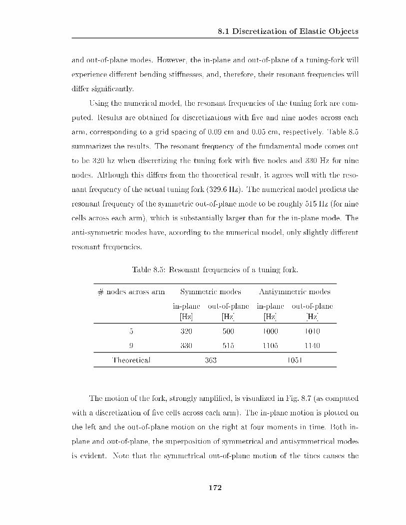
8.1 Discretization of Elastic Objects
and out-of-plane modes. However, the in-plane and out-of-plane of a tuning-fork will
experience di�erent bending sti�nesses, and, therefore, their resonant frequencies will
di�er signi�cantly.
Using the numerical model, the resonant frequencies of the tuning fork are com-
puted. Results are obtained for discretizations with �ve and nine nodes across each
arm, corresponding to a grid spacing of 0.09 cm and 0.05 cm, respectively. Table 8.5
summarizes the results. The resonant frequency of the fundamental mode comes out
to be 320 hz when discretizing the tuning fork with �ve nodes and 330 Hz for nine
nodes. Although this di�ers from the theoretical result, it agrees well with the reso-
nant frequency of the actual tuning fork (329.6 Hz). The numerical model predicts the
resonant frequency of the symmetric out-of-plane mode to be roughly 515 Hz (for nine
cells across each arm), which is substantially larger than for the in-plane mode. The
anti-symmetric modes have, according to the numerical model, only slightly di�erent
resonant frequencies.
Table 8.5: Resonant frequencies of a tuning fork.
# nodes across arm Symmetric modes Antiymmetric modes
in-plane out-of-plane in-plane out-of-plane
[Hz] [Hz] [Hz] [Hz]
5 320 500 1000 1010
9 330 515 1105 1140
Theoretical 363 1051
The motion of the fork, strongly ampli�ed, is visualized in Fig. 8.7 (as computed
with a discretization of �ve cells across each arm). The in-plane motion is plotted on
the left and the out-of-plane motion on the right at four moments in time. Both in-
plane and out-of-plane, the superposition of symmetrical and antisymmetrical modes
is evident. Note that the symmetrical out-of-plane motion of the tines causes the
172

8.1 Discretization of Elastic Objects
In-Plane Out-of-Plane
Figure 8.7: The motion of a tuning fork.
tuning fork to rotate back and forth about its axis, due to the fact that the rotational
momentum must be conserved.
173

8.2 Resonance Behavior of a Buried Land Mine
8.2 Resonance Behavior of a Buried Land Mine
To investigate the resonant oscillations at the location of a buried land mine in more
detail, a mine model has been developed that more closely resembles the structure
of an actual mine. The re�ned mine model is shown in Fig. 8.8. The mine model
includes the details of the mine that are believed to have an impact on the mine's
resonant behavior: the explosives, the plastic case, the rubber pressure plate, and the
air chambers. The model has similar dimensions as an actual TS-50 anti-personnel
mine (see Fig. 7.9). The diameter of the mine is about 8 cm, and its overall height
is 4 cm. The material properties that are assumed for the various parts of the mine
are summarized in Table 8.6. The grid spacing for the �nite-di�erence grid is chosen
to be �x = �y = �z = 0:1 cm. At least two cells are placed across each structural
detail of the mine. The mine's case, at its thinnest spot, is discretized by three cells
across.
Table 8.6: Material properties of the parts of the detailed mine model.
Shear Wave Pressure Wave Material
Speed Speed Density
cS [m/s] cP [m/s] � [kg/m3]
Explosives 1340 2480 1610
Air 0 330 1.3
Plastic Case 1100 2700 1200
Pressure Plate 500 800 1000
To incorporate the features of an actual mine, a much �ner grid than used pre-
viously must be employed in the numerical model. With such a grid, the entire space
including the transducer on the surface and the buried mine cannot be modeled,
because the requirements in computer memory and computation time would be im-
mense. Therefore, with the �ne grid the elastic wave �elds are computed only in the
174
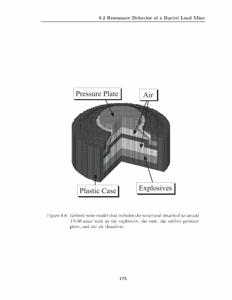
8.2 Resonance Behavior of a Buried Land Mine
AirPressure Plate
Plastic Case Explosives
Figure 8.8: Re�ned mine model that includes the structural details of an actualTS-50 mine such as the explosives, the case, the rubber pressureplate, and the air chambers.
175

8.2 Resonance Behavior of a Buried Land Mine
immediate surrounding of the mine. A grid with 120� 60� 120 cells is used, yielding
an e�ective solution space of 10 cm by 10 cm by 10 cm (because a PML of 10 cells is
employed and the symmetry in the y-direction is exploited, reducing the size of the
numerical grid by a factor of 2). The time step becomes, according to the Courant
condition, �t = 2:138 � 10�7 s. About 117,000 times steps are needed to compute
the wave �elds for 25 ms, requiring a computation time of about �ve hours and 23
minutes on the Beowulf PC cluster using 28 processors.
In the surrounding of the mine, the soil can be roughly approximated as homo-
geneous. Therefore, for all results presented in the following, the material properties
in the ground are assumed constant throughout the medium. Instead of modeling
the transducer on the surface, a vertically polarized plane shear wave is injected from
the left. For this, the total-�eld/scattered-�eld formulation as described in Sec. 4.3
is used. The excitation is a di�erentiated Gaussian pulse with a center frequency of
1 kHz and, thus, has a wider bandwidth than the excitation used previously. A plane
shear wave is chosen, because it resembles the incident guided shear wave and the
Rayleigh surface wave that, as observed previously, are excited by the transducer on
the surface. The scenario is schematically depicted in Fig. 8.9.
The interaction of an incident plane shear wave with a buried mine as com-
puted with the detailed mine model is illustrated in Fig. 8.10. The vertical particle
displacement on the surface plane (top) and on a cross section through the ground
(bottom) is shown at four instants in time. A color scale ranging from black to white
is employed. The mine is buried 2 cm beneath the surface. The material properties
in the ground are assumed to be � = 1400 kg/m3, cP = 250 m/s, and cS = 80 m/s.
In Fig. 8.10, resonant oscillations are seen to be excited at the buried mine. The
oscillations appear to be mainly due to the motion of the thin soil layer above the mine
and the rubber pressure plate of the mine. The oscillations decay as time progresses.
The surface motion appears to be composed of at least two di�erent modes. At T1
and T3, the motion is dominated by a mode describing an upward and downward
motion of the surface above the mine. At T4, a mode causing a rocking motion of the
176
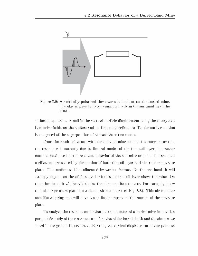
8.2 Resonance Behavior of a Buried Land Mine
Figure 8.9: A vertically polarized shear wave is incident on the buried mine.The elastic wave �elds are computed only in the surrounding of themine.
surface is apparent. A null in the vertical particle displacement along the rotary axis
is clearly visible on the surface and on the cross section. At T2, the surface motion
is composed of the superposition of at least these two modes.
From the results obtained with the detailed mine model, it becomes clear that
the resonance is not only due to exural modes of the thin soil layer, but rather
must be attributed to the resonant behavior of the soil-mine system. The resonant
oscillations are caused by the motion of both the soil layer and the rubber pressure
plate. This motion will be in uenced by various factors. On the one hand, it will
strongly depend on the sti�ness and thickness of the soil layer above the mine. On
the other hand, it will be a�ected by the mine and its structure. For example, below
the rubber pressure plate lies a closed air chamber (see Fig. 8.8). This air chamber
acts like a spring and will have a signi�cant impact on the motion of the pressure
plate.
To analyze the resonant oscillations at the location of a buried mine in detail, a
parametric study of the resonance as a function of the burial depth and the shear wave
speed in the ground is conducted. For this, the vertical displacement at one point on
177
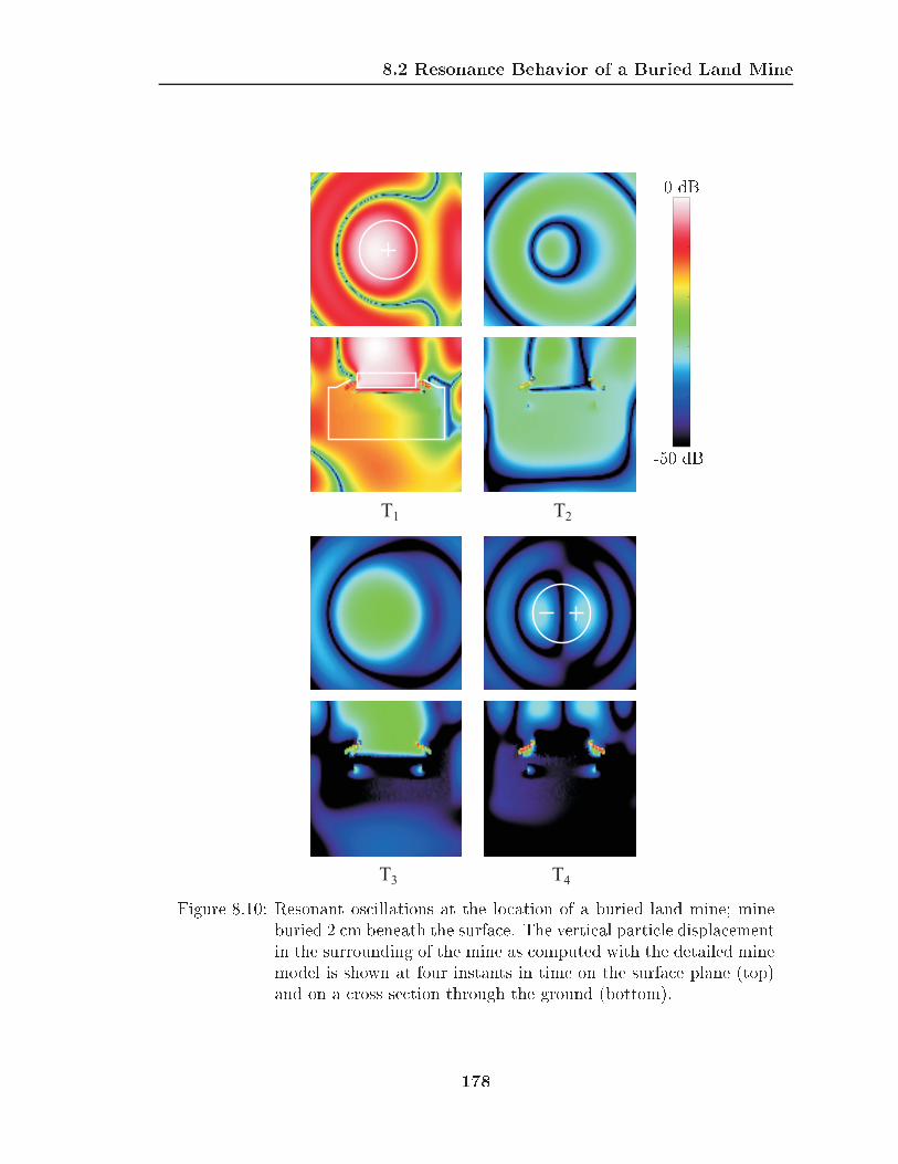
8.2 Resonance Behavior of a Buried Land Mine
T2
T3 T4
T1
0 dB
-50 dB
Figure 8.10: Resonant oscillations at the location of a buried land mine; mineburied 2 cm beneath the surface. The vertical particle displacementin the surrounding of the mine as computed with the detailed minemodel is shown at four instants in time on the surface plane (top)and on a cross section through the ground (bottom).
178

8.2 Resonance Behavior of a Buried Land Mine
the surface above the mine is computed in the time domain. A point is picked that lies
1 cm o� the vertical symmetry axis of the mine. The motion is Fourier transformed
from the time domain into the frequency domain, and, by dividing by the Fourier
transform of the incident pulse, the transfer function is determined. From the transfer
function, the resonant frequencies of the vertical particle motion can be identi�ed.
For the parametric study, shear wave speeds in the range from 40 m/s up to 150 m/s
are considered in order to determine the response for fairly loose as well as rather
sti� soils. These values are representative for the shear wave speeds at the surface for
many common soil types. The pressure wave speed and the material density will be
kept constant throughout the study, at cP = 250 m/s and � = 1400 kg/m3.
Fig. 8.11 shows the transfer function for a mine buried 1 cm beneath the surface.
The shear wave speed in the ground is assumed to be 40 m/s. In the range up to
2.1 kHz, two resonant peaks can be distinguished. The two peaks correspond to two
modes of the surface motion. The �rst mode has a resonant frequency of about 691 Hz
and corresponds to the up- and downward motion of the surface. The second mode,
at about 1.373 kHz, describes the rocking motion. The surface motion associated
with the modes is illustrated in Fig. 8.11. The two modes that are excited within the
soil-mine system are similar in shape to the �rst two modes of a thin circular disc
that is rigidly clamped along its edge [58, 79]. However, the analogy to the circular
disc cannot be used to accurately predict the resonant frequencies of the soil-mine
system, because along its edge the soil layer in the model is not rigidly �xed and
the structure of the mine has a signi�cant impact on the resonance. An additional
peak at about 2 kHz is apparent in Fig. 8.11. The origin of this peak, however, is
not clearly understood. It might be due to a resonance in the mine itself. Further
studies, beyond the scope of this work, are needed to explore the resonant behavior
at higher frequencies.
To explore the resonance for mines buried in di�erent types of soil, the resonant
behavior is determined as a function of the shear wave speed in the ground and the
burial depth of the mine. Fig. 8.12 shows the transfer function as a function of the
179

8.2 Resonance Behavior of a Buried Land Mine
0 1000 2000Frequency [Hz]
Dis
pla
cem
ent
Figure 8.11: Transfer function of a point on the surface above the mine; mineburied at 1 cm; cS = 40 m/s. The two resonant peaks correspondto two distinct modes of the vertical surface motion.
180

8.2 Resonance Behavior of a Buried Land Mine
shear wave speed in the ground with the burial depth of the mine �xed at 2 cm (top)
and as a function of the burial depth with the shear wave speed kept constant at
40 m/s (bottom). It is apparent that for increasing shear wave speed the resonant
frequencies of the �rst and second peak are shifted upwards in frequency. At the
same time, the amplitudes of the peaks drop, and the quality factor of the modes
is degraded. For increasing burial depth, the two resonant peaks are shifted slightly
downwards, and their amplitudes drop drastically. For the mine at 4 cm, the second
resonant peak is not distinguishable any more.
To summarize the results, the resonant frequency and the quality factor of the
�rst resonant peak are plotted in two parametric graphs as a function of the shear
wave speed in the ground with the burial depth as a parameter. The results are shown
in Fig. 8.13. Note that, by varying the shear wave speed in the ground while keeping
the material density constant, e�ectively the sti�ness in the ground is being varied.
Thus, in these plots the resonant behavior is shown essentially as a function of the
sti�ness in the ground. The top line in each plot corresponds to the mine at a burial
depth of 1 cm. Qualitatively, it can be seen that the resonant frequency increases
with shear wave speed and decreases with burial depth. The quality factor of the
resonance decreases with both shear wave speed and burial depth. The decrease in
the quality factor of the resonance with both increasing sti�ness and burial depth
indicates that the resonance is dampened. The only damping mechanism a�ecting
the resonance within the model is the radiation of energy into the surrounding soil.
The coupling of the thin soil layer above the mine to the surrounding soil increases
with the sti�ness and the thickness of the layer. Thus, the energy that is radiated
increases, and the damping of the resonance is enhanced.
Resonant oscillations at the location of a buried land mine have also been ob-
served experimentally. Fig. 8.14 shows measured results for an actual TS-50 mine
buried 1 cm beneath the surface. In the top graph the measured transfer function of
the surface motion at a point above the mine is plotted, whereas in the bottom graph
various numerically determined transfer functions are shown. The curves are seen
181

8.2 Resonance Behavior of a Buried Land Mine
0 1000 2000Frequency [Hz]
Dis
pla
cem
ent
cS = 40 m/s
c
c
c
c
S
S
S
S
= 60 m/s
= 80 m/s
= 100 m/s
= 150 m/s
(a)
0 1000 2000Frequency [Hz]
Dis
pla
cem
ent
d
d
= 1 cm
= 2 cm
= 3 cm
= 4 cm
d
d
(b)
Figure 8.12: Surface motion at a point above the mine; transfer functions. (a)Mine buried 2 cm beneath the surface, variable shear wave speed;(b) shear wave speed cS = 40 m/s, variable depth.
182

8.2 Resonance Behavior of a Buried Land Mine
40 60 80 100 120 140 160
Shear Wave Speed [m/s]
d = 1 cmd = 2 cmd = 3 cmd = 4 cmd = 5 cmd = 6 cm
Qu
alit
yF
acto
r,Q
0
4
8
12
200
400
600
800
1000
1200
1400
1600
1800
40 60 80 100 120 140 160
Shear Wave Speed [m/s]
Res
on
ant
Fre
qu
ency
[Hz]
d = 1 cmd = 2 cmd = 3 cmd = 4 cmd = 5 cmd = 6 cm
Figure 8.13: Parametric graphs of the resonant frequency and the quality factorof the �rst resonant peak as a function of the shear wave speed inthe ground with the burial depth as a parameter.
183

8.2 Resonance Behavior of a Buried Land Mine
to be quite di�erent. The measured transfer function exhibits two resonant peaks
at about 450 Hz and 700 Hz. The second peak is very weak, and the response is
negligible for frequencies higher than about 1 kHz. The numerical transfer functions
for four cases are plotted: for a mine at 1 cm assuming shear wave speeds in the
ground of 20 m/s, 30 m/s and 40 m/s, and for a mine at 2 cm assuming a shear
wave speed in the ground of 40 m/s. The best resemblance with the experimental
data is obtained for the �rst of these cases. When assuming a burial depth of 1 cm
and a shear wave speed of 20 m/s, two peaks occur, approximately at 400 Hz and
at 750 Hz (bottom, solid curve). Contrary to the experimental result, however, the
numerical results indicate a signi�cant response at high frequencies. It is believed
that the di�erences between experimental and numerical results are mainly due to
uncertainties in the experimental model and to non-linear e�ects occurring in the
sand. Earlier, an estimate of the wave speed variation with depth has been shown
(see Fig. 7.1). This depth pro�le might be especially inaccurate at and close to the
surface, predicting wave speeds at the surface that are far too large. Nominally, in the
experiment the mine is buried at 1 cm. However, the actual burial depth of the mine
might di�er, because the level of accuracy that can be achieved when placing the mine
in the ground is limited. Thus, the actual burial depth of the mine will lie roughly
within �0:5 cm of the nominal burial depth. The sand in the experiments behaves in
a strongly non-linear way. The non-linear e�ects dampen the high frequency compo-
nents of the elastic waves and e�ectively suppress frequency components above about
500 Hz. Due to the resonant oscillations at a buried mine, the surface motion above
the mine is ampli�ed and driven strongly into the non-linear regime, thus enhancing
the e�ects of loss and non-linearities. To obtain a better agreement of experiment
and numerical simulation, the experiment must be repeated using smaller drive levels,
thus exciting elastic waves with a smaller amplitude to achieve operation in the linear
regime of the sand.
The numerically determined transfer functions exhibit ripples at low frequencies.
These ripples are numerical artifacts and are due to the fact that the resonant response
184

8.3 Excitation by a Pressure Wave
0 1000 2000Frequency [Hz]
Dis
pla
cem
ent
1 cm, 20 m/s
1 cm
1 cm
cS �, 0 m/s
, 0 m/s
2 cm, 0 m/s
c
c
c
S
S
S
���������
Measured
Figure 8.14: Experimental results for a mine buried at 1 cm; transfer function.
has not been computed long enough. Within the time window for which the wave
�elds are computed, the response of the mine has not completely decayed, and thus
the numerical transfer function exhibits the true response of the mine convolved
with the shape of the time window. In other words, the transfer function in the
frequency domain is the product of the Fourier transforms of the true response and
the rectangular time window (i. e., a sinc-function), causing the ripples visible in
Fig. 8.14.
8.3 Excitation by a Pressure Wave
In the mine detection system that is investigated in this work, the elastic waves are
excited by an electrodynamic transducer placed on the surface of the ground. Such a
185

8.3 Excitation by a Pressure Wave
transducer will launch predominantly shear and Rayleigh surface waves which propa-
gate along the surface of the ground and interact with the buried mine. This scenario
resembles the case that has been studied in the last section, where the buried mine
was excited by a shear wave incident from the side. A plane shear wave incident onto
the mine from the side will excite resonant oscillations at the mine similar to the ones
excited by a Rayleigh wave or a guided shear wave as observed in Chapter 7. Di�erent
types of excitations are, however, possible in an acoustic mine detection system. In a
di�erent approach, elastic waves in the ground are excited by a loudspeaker mounted
above the surface [3, 10]. The loudspeaker radiates acoustic pressure waves, which
impinge upon the surface of the ground and couple primarily into pressure waves in
the ground. The pressure waves do not propagate along the surface, but rather are
directed vertically into the ground. To study this form of excitation, the response of
a buried mine to pressure waves being incident from above the mine is analyzed using
the detailed mine model.
Fig. 8.15 shows the con�guration schematically. A pressure wave is vertically in-
cident upon the buried mine. A di�erentiated Gaussian pulse with a center frequency
of 1 kHz is used as excitation. As before, the material properties are assumed to be
homogeneous around the mine.
Fig. 8.16 shows the transfer function of a point on the surface above the mine
for the excitation with a shear wave incident from the side (solid line) and with a
pressure wave incident from above (dashed line). The mine is buried 1 cm beneath
the surface, and the shear wave speed in the ground is cS = 40 m/s. The di�erences
are apparent. As described previously, the shear wave excites two resonant peaks in
the range up to 2.1 kHz. The pressure wave, however, excites only the �rst resonant
mode. This is readily explained by noting the symmetry of the incident pressure
wave. The plane pressure wave is symmetric with respect to the vertical axis of the
mine. Thus, it will excite only modes that are equally symmetric. The second mode
excited by the shear wave is asymmetric with respect to the mine's axis, as visible
in Fig. 8.11, and consequently it is not excited by the pressure wave incident from
186

8.3 Excitation by a Pressure Wave
Figure 8.15: A pressure wave is vertically incident on the buried mine.
above.
Fig. 8.17 shows the transfer function due to the excitation with an incident
pressure wave in (a) as a function of the shear wave speed in the ground for the
mine buried at 2 cm and in (b) as a function of the burial depth for a shear wave
speed of 40 m/s. For increasing shear wave speed and, thus, for increasing shear
sti�ness, the resonant frequency of the mode excited by the pressure wave is shifted
upwards in frequency and the amplitude of the resonance decreases, causing the
quality factor of the resonance to be degraded. When increasing the burial depth,
the resonant frequency is shifted slightly downwards in frequency and the amplitude
drops, indicating that the resonance is increasingly dampened. The resonant mode
that is excited by the pressure wave behaves in a similar way as the �rst resonant
mode excited by the shear wave incident from the side (see Fig. 8.12). The second
resonant mode that is excited by the shear wave, however, is not apparent for the
pressure wave excitation. Note that the resonant peak for the mine at 3 cm is barely
distinguishable and for the mine at 4 cm has vanished or is superimposed by other
187

8.3 Excitation by a Pressure Wave
0 1000 2000Frequency [Hz]
Dis
pla
cem
ent
Pressure Wave from AboveShear from Side
Figure 8.16: Transfer functions of the surface motion due to the excitation withshear wave from the side and a pressure wave from above.
e�ects.
The results are summarized in Fig. 8.18 in parametric graphs showing the res-
onant frequency and the quality factor of the �rst mode as a function of the shear
wave speed in the ground with the burial depth as a parameter. Burial depths of
1 cm, 2 cm and 3 cm are considered. For larger burial depths, the �rst resonant mode
is not clearly identi�able, and other resonant e�ects of the mine become dominant.
The results are similar to the results for the shear wave excitation. The resonant
frequency increases with the shear wave speed in the ground and decreases with the
burial depth. The quality factor of the resonance decreases with both shear wave
speed and burial depth.
188

8.3 Excitation by a Pressure Wave
0 1000 2000Frequency [Hz]
Dis
pla
cem
ent
cS = 40 m/s
c
c
c
c
S
S
S
S
= 60 m/s
= 80 m/s
= 100 m/s
= 150 m/s
(a)
0 1000 2000Frequency [Hz]
Dis
pla
cem
ent
d
d
= 1 cm
= 2 cm
= 3 cm
= 4 cm
d
d
(b)
Figure 8.17: Surface motion at a point above the mine; tranfer functions. Exci-tation with a pressure wave from above. (a) Mine buried 2 cm be-neath the surface, variable shear wave speed; (b) shear wave speedcS = 40 m/s, variable depth.
189

8.3 Excitation by a Pressure Wave
40 60 80 100 120 140 160
Shear Wave Speed [m/s]
d = 1 cmd = 2 cmd = 3 cmd = 4 cmd = 5 cmd = 6 cm
Qu
alit
yF
acto
r,Q
0
4
8
12
200
400
600
800
1000
1200
1400
1600
1800
40 60 80 100 120 140 160
Shear Wave Speed [m/s]
Res
on
ant
Fre
qu
ency
[Hz]
d = 1 cmd = 2 cmd = 3 cmd = 4 cmd = 5 cmd = 6 cm
Figure 8.18: Parametric graphs of the resonant frequency and the quality factorof the �rst resonant mode as a function of the shear wave speed inthe ground with the burial depth as a parameter. Pressure waveexcitation.
190
CHAPTER 9
Experiments
In experimental measurements, elastic waves propagating along the surface of the
ground have been observed to be dispersed. The dispersion is believed to be largely
due to the material properties in the ground being inhomogeneous. As has been
argued earlier (see Chapter 7), a Rayleigh surface wave will be dispersed if the wave
speeds in the ground are a function of depth, because the reach of the Rayleigh wave
into the ground depends on frequency, and, thus, di�erent frequency components
of the Rayleigh wave will experience di�erent wave speeds. To explore the wave
propagation in the ground, the elastic wave �elds in the ground are measured.
The laboratory experiments are performed in a large sand-�lled tank. If the
elastic wave �elds in sand are assumed to behave in a linear manner, the material
properties of sand can be described by three independent constants: the material
density �, the shear wave speed cS, and the pressure wave speed cP . In this chapter,
procedures to measure these quantities as a function of depth are described, and
measurement results are presented.
The measurement of soil properties has been treated extensively in the literature
[81] { [83]. The signal processing techniques applied in this chapter are adapted from
Oppenheim and Schafer [84] and Smith et al. [62].
191
9.1 Measuring the Water Content in the Ground
9.1 Measuring the Water Content in the Ground
Before a measurement, the sand in the laboratory tank is usually uniformly wetted
and packed. This is primarily done to minimize the loss e�ects at the surface and to
improve the lateral uniformity of the material properties in the tank. A water table
is maintained within the tank to approximate realistic conditions. Consequently, the
water content within the sand is largely inhomogeneous with depth.
Changes in the water content with depth might have a signi�cant impact on the
wave propagation in the ground. If the water in the ground is assumed to primarily
�ll in the voids of the sand matrix (which is constituted by the grains of the sand),
the water content will not in uence the mass of the sand per volume, but it will
a�ect the overall mass per volume, thus changing the material density in the ground.
Additionally, the water content in the ground will a�ect the cohesion between the
grains of the sand. A change in the cohesion will primarily in uence the wave speeds
in the ground, because an increase in the cohesion is synonymous with an increase in
the sti�ness.
To measure the water content within the sand, an easy and straightforward
procedure has been applied. Various samples of the sand were taken at a range of
depths. The samples were weighed using a conventional scale accurate to 0.01 g and
then dried to remove the water. A conventional oven at 400 degrees Fahrenheit was
used to dry the samples, baking the samples for about twelve hours. The samples
were �nally weighed again. The weight di�erence between the initial sample and
the dry sample represents the water content. Table 9.1 lists the results of the water
content measurement, and Fig. 9.1 shows the water content in percent of the mass of
sand as a function of depth. The water content was calculated as
Water Content [% mass] =W1 �W2
W2
� 100; (9.1)
where W1 indicates the weight of the sample before drying, andW2 is the weight after
drying. In Eq. (9.1), the atmospheric pressure and the pressure within the sand were
neglected. Note that the water table has been found to lie at a depth of about 52 cm.
192

9.1 Measuring the Water Content in the Ground
0 10 20 30 40 50Depth [cm]
5
10
15
20
25
Wat
erC
on
ten
t[%
]
Figure 9.1: Water content (mass percent) as a function of depth.
In the water table, the mass of the water per volume is about 22 % of the mass of
sand per volume.
As stated above, if the water �lls in the matrix of the sand, the mass of the sand
per volume will be constant, but the overall mass per volume will change due to the
additional mass of the water. The change in the material density is then
� = �sand +Water Content [% mass]
100�sand: (9.2)
The density of dry sand is assumed to be �sand = 1400 kg/m3. The resulting material
density as a function of depth is graphed in Fig. 9.2.
The depth dependence of the material density might have an e�ect on the other
material properties. For example, if the sti�ness in the ground is assumed to be
constant, an increase in the material density will cause a decrease in the wave speeds.
193

9.1 Measuring the Water Content in the Ground
Table 9.1: Measurement of the water content as a function of depth.
Depth W1 W2 Water Content
[cm] [g] [g] [% mass]
0 127.10 125.31 1.44
2 140.93 138.09 2.06
4 167.66 163.62 2.46
7 164.60 160.40 2.61
10 148.85 143.50 3.70
13 164.04 156.16 4.90
16 151.87 144.25 5.15
19 155.18 146.65 5.61
22 191.96 179.75 6.48
25 142.04 132.33 6.99
28 156.24 144.64 7.60
31 166.07 151.03 9.23
34 162.36 145.65 10.50
37 228.01 199.95 12.51
40 228.92 196.19 14.50
43 196.63 166.33 15.64
46 234.54 195.04 17.12
49 233.81 190.35 18.85
52 203.94 163.34 20.25
55 153.06 119.96 22.08
194

9.1 Measuring the Water Content in the Ground
0 10 20 30 40 50Depth [cm]
1450
1500
1550
1600
1650
1700
1750
Mat
eria
lD
ensi
ty[k
g/m
]3
1400
Figure 9.2: Material density as a function of depth.
195
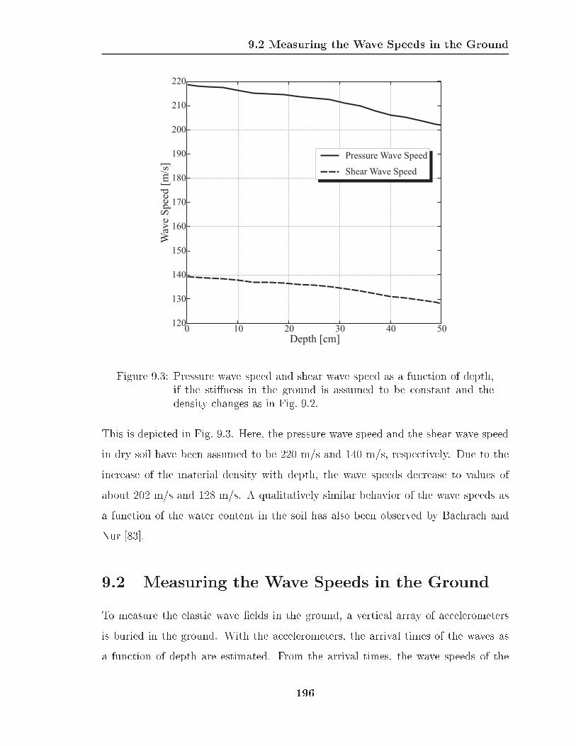
9.2 Measuring the Wave Speeds in the Ground
0 10 20 30 40 50
130
120
140
150
160
170
180
190
200
210
220
Pressure Wave Speed
Shear Wave SpeedW
ave
Sp
eed
[m/s
]
Depth [cm]
Figure 9.3: Pressure wave speed and shear wave speed as a function of depth,if the sti�ness in the ground is assumed to be constant and thedensity changes as in Fig. 9.2.
This is depicted in Fig. 9.3. Here, the pressure wave speed and the shear wave speed
in dry soil have been assumed to be 220 m/s and 140 m/s, respectively. Due to the
increase of the material density with depth, the wave speeds decrease to values of
about 202 m/s and 128 m/s. A qualitatively similar behavior of the wave speeds as
a function of the water content in the soil has also been observed by Bachrach and
Nur [83].
9.2 Measuring the Wave Speeds in the Ground
To measure the elastic wave �elds in the ground, a vertical array of accelerometers
is buried in the ground. With the accelerometers, the arrival times of the waves as
a function of depth are estimated. From the arrival times, the wave speeds of the
196

9.2 Measuring the Wave Speeds in the Ground
di�erent wave types can be determined.
9.2.1 Experimental Set-Up
Fig. 9.4 gives a schematic overview of the measurement setup. The elastic waves
are excited by a transducer placed on the surface of the ground. A vertical array of
accelerometers is buried in the ground. Ten bi-axial accelerometer pairs measuring
the horizontal and vertical particle acceleration are used, thus providing 20 signals.
The shallowest accelerometer pair is placed at a depth of 5 cm, the deepest at 50 cm,
and the spacing between the accelerometer pairs is 5 cm. The accelerometers are
powered by a power supply decoupling unit supplying a DC voltage of 27 Volts. The
20 measured signals are ampli�ed by a preampli�er with a constant gain of 320 and
fed into a computer through a data acquisition card.
The accelerometers (manufactured by Vibra-Metrics, Model 9002 A) are
coated to improve their water resistance and enclosed in syntactic foam, making
the accelerometers neutrally buoyant in water. Two accelerometers were orthogo-
nally mounted on a piece of plexiglas, raising the material density of the formation
to roughly the density of sand (� 1400 kg/m3).
The drive signal fed to the transducer is a frequency modulated chirp with a
length of 8 s and has a frequency range from 30 Hz to 2 kHz. Because the response
to the chirp is rather complicated to interpret, the measured signal is processed. For
each channel, the transfer function is determined and convolved with a di�erentiated
Gaussian pulse.
Fig. 9.5 illustrates the signal processing. A chirp is supplied to the transducer
(Drive Signal, top right). Ten accelerometer pairs measure the acceleration in the
ground, providing 20 signals (Accelerometer Signal, top left). The accelerometer
signal and the drive signal are Fourier transformed. By dividing the Fourier transform
of the accelerometer signal by the Fourier transform of the drive signal, the transfer
function for each channel is obtained (Transfer Function, third from top on the left).
197

9.2 Measuring the Wave Speeds in the Ground
Transducer
5 cm
Accelerometers
20 Output Channels
Sand
(a)
Power DecouplingUnit (PCU)
PreamplifierGain = 320
Data Acquisition Card PC
Drive Signal(Chirp, ~ 8 s, 30 Hz .. 2 kHz)
Bandpass(30 Hz .. 2 kHz)
Amplifier
ElectrodynamicTransducer
Accelerometers
(b)
Figure 9.4: Set-up for accelerometer measurements. (a) Transducer and ac-celerometer array; (b) measurement set-up.
198

9.2 Measuring the Wave Speeds in the Ground
The transfer function is multiplied by the Fourier transform of a Reference Signal
(di�erentiated Gaussian pulse, bottom right) and inverse-Fourier transformed. In
this way, the signal due to the reference signal is obtained, i. e., the signal that would
have been measured if the reference signal had been fed to the transducer instead of
the chirp.
9.2.2 Measurement Procedure
Fig. 9.6 schematically shows the arrangement of the transducer and the accelerome-
ters in the laboratory tank. The accelerometer measurements were repeated numer-
ous times. The accelerometers were �rst buried by digging a large hole ( � 50 cm
in diameter) using a conventional shovel. The hole was re�lled and repacked, as the
accelerometers were positioned in the ground. The measured results were noisy, and
re ections occurred which could be attributed primarily to the disturbance of the sand
due to the hole that was dug in the process of burying the accelerometers. To improve
the measurements, the accelerometers were removed from the hole, and the soil in the
entire sand box was repacked by using a commercial packing machine (Vibco plate
compactor). According to its speci�cations, the packing machine packs the sand well
down to a depth of about 30 cm. The accelerometers were then buried by drilling
a bore-hole-like cylindrical hole with a diameter of about 5 cm. The accelerometers
were carefully aligned in the hole and regularly spaced at depths between 5 cm and
50 cm. The water table was measured to be at about 52 cm, and thus the deepest
accelerometer was placed just above the water table. The particle acceleration in
the ground was measured for various transducer positions with respect to the burial
hole. The transducer was placed at distances of 0.5 m, 1 m and 1.5 m from the
location of the accelerometers and was displaced in two directions to investigate the
e�ects of local inhomogeneities in the sand. The measurements were repeated sev-
eral times, studying various conditions. The measurements were performed directly
after burying the accelerometers and repeated throughout the following days, for a
199

9.2 Measuring the Wave Speeds in the Ground
Reference Signal
Fourier TransformFourier Transform
Fourier TransformInverse Fourier Transform
0 5 10 15 20 25 30 35 40 45 50
Time [ms]
0 2 4 6 8Time [s]
0 2 4 6 8Time [s]
0 1000 2000 3000 4000Frequency [Hz]
0 1000 2000Frequency [Hz]
0 1000 2000Frequency [Hz]
Signal due to excitation withdifferentiated Gaussian pulse
0 1000 2000 3000 4000Frequency [Hz]
Transfer Function
Accelerometer Signal(24 Channels)
Drive Signal
Figure 9.5: Signal processing: the accelerometer signal is Fourier transformed,divided by the Fourier transform of the drive signal (chirp), mul-tiplied by the reference signal (di�erentiated Gaussian pulse), andthen inverse-Fourier transformed.
200
9.2 Measuring the Wave Speeds in the Ground
wet surface as well as for a dry surface. To investigate the in uence of the burial
hole, the accelerometers were removed and reburied at a di�erent location, and the
measurements were repeated.
Before burying the accelerometers, the accelerometers were calibrated. The
sensitivity of all accelerometers was found to lie within �10 % of the mean sensitivity.
The di�erences in the accelerometer response were adjusted for during the signal
processing of the measured signals.
Minimizing the disturbance of the sand by burying the accelerometers in a bore-
hole-like hole clearly improved the measurement results, eliminating re ections from
local inhomogeneities due to the accelerometer burial. The measurements with the
bore hole arrangement were found to be largely independent of the time that had
passed after the burial of the accelerometers, of the state of the surface (dry or wet),
and of the burial location of the accelerometers. No re ections from the water table
or the tank walls could be observed. It is believed that a residual content of air is
present below the water table, causing the values of the wave speeds above and below
the water table to be comparable in size [83]. In that case, the re ections from the
water table are negligible. The re ections from the tank walls are believed to be
largely attenuated by the lossy sand.
Various complications arose during the measurements. Several accelerometers
became erratic during the initial measurements. This was believed to be due to
damages in the sealed cases of the accelerometers, allowing water to seep into the ac-
celerometers. To improve their sealing, the accelerometers were coated with multiple
layers of polyurethane varnish. With the coating, the accelerometers were buried in
the ground for an extended period of time without a noticeable deterioration in their
performance.
201

9.2 Measuring the Wave Speeds in the Ground
Sand Box
Accelerometers
50 cm
1.5 m
5.8 m
6.1 m
52 cm
Transducer
Water Table
Figure 9.6: Accelerometer and transducer positions in the laboratory tank.
202

9.2 Measuring the Wave Speeds in the Ground
9.2.3 Results
Using the accelerometer array, the elastic wave �elds in the ground are measured
as a function of depth. Fig. 9.7 shows the wave �elds as a function of depth and
time for a lateral distance of 1.5 m between transducer and accelerometer location.
At the top, the vertical and horizontal particle acceleration are graphed on a linear
scale. The two plots below show the �eld components on a logarithmic scale using a
dynamic range of 35 dB. The same color map as earlier is employed. The excitation
is a di�erentiated Gaussian pulse with a center frequency of 450 Hz, launched by the
transducer at 0 ms.
Five wave fronts are distinguishable. The fastest wave front (P) is the pressure
wave. Due to the spherical shape of the propagating waves, the wave front recorded
by the vertical array is curved. Note that at the surface the pressure wave arrives
later than in the ground, indicating that the pressure wave speed at the surface is
smaller than within the ground. The second wave front (LS), primarily visible in the
horizontal �eld component, is the leaky surface wave. The leaky surface wave appears
as a straight line that originates at the surface. The third wave front (S) represents
the shear wave in the ground. The fourth wave (GS) corresponds to the guided shear
wave and is strongest close to the surface. The slowest wave is the Rayleigh surface
wave (R). Note that the Rayleigh surface wave at a depth of 5 cm (i. e., the top line in
Fig. 9.7) has a prograde particle motion, indicated by the vertical component leading
the horizontal component in phase, rather than a retrograde motion as was found
earlier for a Rayleigh wave at the surface. This is due to the fact that the shallowest
accelerometer is placed at a depth of 5 cm and not at the surface. As it was shown
previously in Fig. 6.2, the particle motion of the Rayleigh wave reverses its direction
at a depth of about 0.2 times the wavelength of the Rayleigh wave. At a frequency of
450 Hz, this equals roughly 3 cm. Thus, at a depth of 5 cm the Rayleigh wave indeed
describes a prograde particle motion, and the measured results are in agreement with
the theoretical prediction.
203
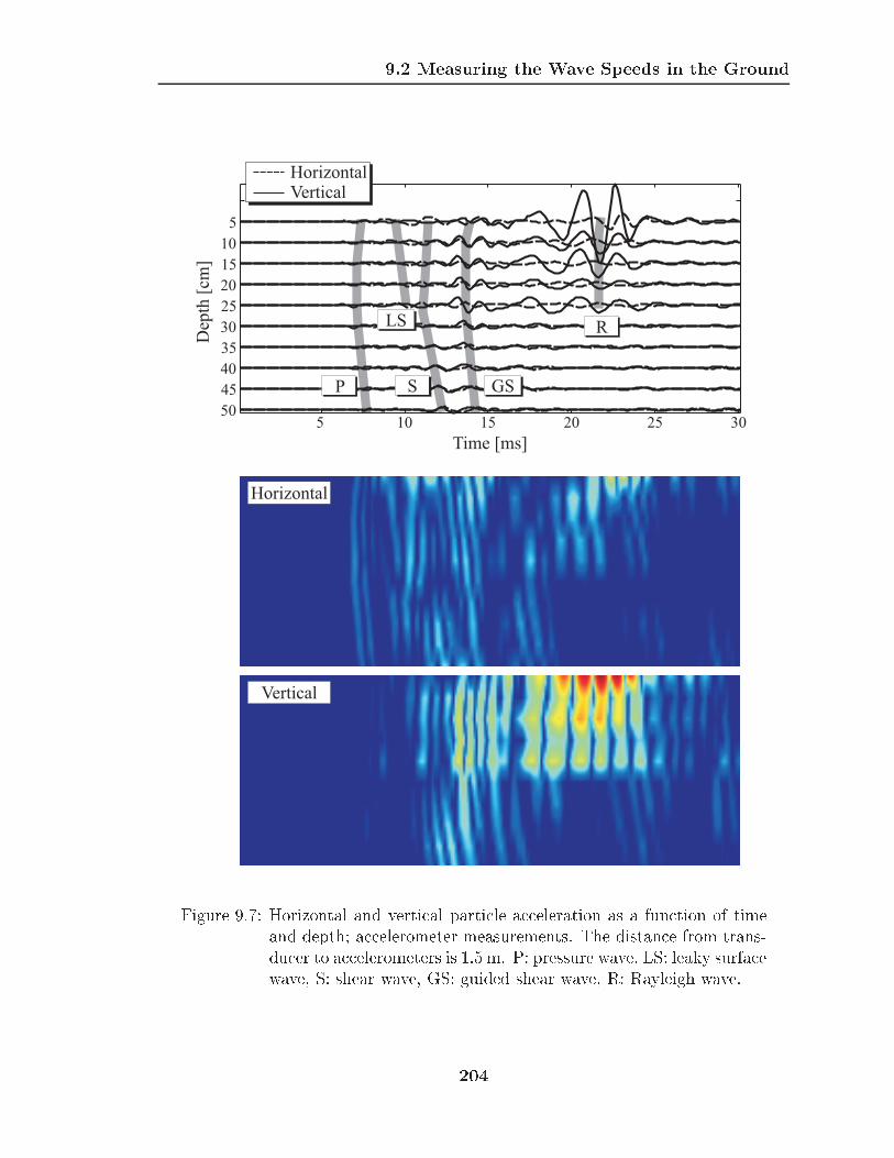
9.2 Measuring the Wave Speeds in the Ground
5 10 15 20 25 3050
45
40
35
30
25
20
15
10
5
Time [ms]
Dep
th[c
m]
PP PS 2 SndGS
2 SndLSRR
Horizontal
Vertical
HorizontalVertical
Figure 9.7: Horizontal and vertical particle acceleration as a function of timeand depth; accelerometer measurements. The distance from trans-ducer to accelerometers is 1.5 m. P: pressure wave, LS: leaky surfacewave, S: shear wave, GS: guided shear wave, R: Rayleigh wave.
204

9.2 Measuring the Wave Speeds in the Ground
From Fig. 9.7, the arrival times of the separate wave fronts can be estimated
as a function of depth. Table 9.2 lists the arrival times for all wave types and the
corresponding wave speeds derived from the arrival times. The wave speeds are
estimated by assuming a direct propagation path, thus neglecting the refraction of
the waves due to the inhomogeneous material properties:
c �pD2 + d2
tarrival; (9.3)
where D is the lateral distance from the transducer to the accelerometers, and d is the
burial depth of the accelerometers. From Table 9.2, the wave speeds of the shear wave
Table 9.2: Measured arrival times and wave speeds: pressure wave front.
Pressure Wave Leaky Wave Shear Wave Guided Shear Wave Rayleigh Wave
Depth Arrival Wave Arrival Wave Arrival Wave Arrival Wave Arrival Wave
Time Speed Time Speed Time Speed Time Speed Time Speed
[cm] [ms] [m/s] [ms] [m/s] [ms] [m/s] [ms] [m/s] [ms] [m/s]
5 7.32 205 9.71 154 10.86 138 14.09 107 21.59 69
10 7.14 211 9.68 155 10.74 140 13.59 111 21.69 69
15 7.07 213 9.65 156 10.67 141 13.59 111 21.59 69
20 7.07 214 9.77 155 10.64 142 13.62 111 21.56 70
25 7.11 214 9.77 156 10.64 143 13.59 112 21.53 70
30 7.07 216 10.58 145 13.78 111
35 7.17 215 10.89 141 13.93 111
40 7.23 215 11.05 141 13.99 111
45 7.32 214 11.11 141 14.36 109
50 7.48 211 11.39 139 14.64 108
and the pressure wave as a function of depth can be deducted in an approximate sense.
The pressure wave speed appears to be slightly smaller at the surface (� 205 m/s at
a depth of 5 cm) than within the ground (� 215 m/s). The shear wave speed in
the ground is roughly 140 m/s. The guided shear wave propagates at a speed of
about 110 m/s, and the Rayleigh wave has a speed of about 70 m/s. The speeds of
shear wave, guided shear wave and Rayleigh wave give indications about the shear
wave speed variation in the ground. From the speed of the Rayleigh wave it can be
205

9.2 Measuring the Wave Speeds in the Ground
concluded that a layer with a rather slow shear wave speed exists close to the surface.
Assuming that the Rayleigh wave speed equals about 0.9 times the shear wave speed
at the surface, the shear wave speed of the surface layer can be estimated to be about
80 m/s. The shear wave front indicates that the shear wave speed beyond the surface
layer is about 140 m/s. The guided shear wave propagates primarily in the region
beyond the surface layer. The guided shear wave arises due to the rapid change in the
shear wave speed in the transition zone between surface layer and the deeper medium.
Because of the change in the shear wave speed, the guided shear wave is refracted
towards the surface, is re ected by the surface, refracted back towards the surface
and so forth. Due to the refraction, the path of the guided shear wave is curved, and
the wave speed of the guided shear wave along the surface is smaller than the shear
wave speed within the ground.
From the wave speeds within the ground, an approximate wave speed pro�le has
been derived. This approximate pro�le was subsequently re�ned by trying to match
numerical data to the measured results and by repeatedly tweaking the depth pro�le
of the wave speeds within the numerical model. The estimated depth pro�le that
yielded best agreement is shown in Fig. 9.8.
The depth pro�le shown in Fig. 9.8 is a crude approximation to to the actual
depth variation of the material properties in the ground. To obtain a more accurate
representation of the depth variation, more sophisticated techniques, such as numer-
ical inversion algorithms, must be employed, which are, however, beyond the scope
of this work.
Fig. 9.9 shows the wave �elds as computed with the numerical model. The par-
ticle displacement is plotted on a linear scale for a transducer-accelerometer distance
of 1.5 m. The arrival times and the curvature of the separate wave fronts agree fairly
well with the experimental results (see Fig. 9.7). The measurements revealed that
at a depth of 5 cm the Rayleigh wave describes a prograde particle motion. The
numerical results predict the same. At the surface (top line), the particle motion for
the Rayleigh wave is retrograde. At a depth of 5 cm, the horizontal motion reverses
206

9.2 Measuring the Wave Speeds in the Ground
0 10 20 30 40 50Depth [cm]
80
100
120
140
160
180
200
220
Wav
eS
pee
d[m
/s]
Pressure Wave Speed
Shear Wave Speed
Figure 9.8: Pressure wave speed and shear wave speed as a function of depth.
207

9.2 Measuring the Wave Speeds in the Ground
5 10 15 20 25 3050
45
40
35
30
25
20
15
10
5
Time [ms]
Dep
th[c
m]
HorizontalVertical
PP PS 2 SndGS
RR2 SndLS
Figure 9.9: Horizontal and vertical particle acceleration as a function of timeand depth; numerical simulation. The distance from transducer toaccelerometers is 1.5 m. P: pressure wave, LS: leaky surface wave,S: shear wave, GS: shear wave, R: Rayleigh wave.
its sign, and thus the particle motion becomes prograde.
In Fig. 9.10, the wave �elds in the ground as computed with the numerical model
are shown and compared to the measured results for three transducer-accelerometer
distances (0.5 m, 1 m, 1.5 m from top to bottom). The dynamic range is 35 dB
for the experimental results (left column) and 50 dB for the numerical results (right
column). Note that the measured results show the particle acceleration, whereas the
numerical results show the particle displacement. The same qualitative behavior is
observed for the experimental and the numerical results. The separate wave fronts
have roughly the same shapes and the same wave speeds. Di�erences can mainly be
observed for the leaky surface wave and the Rayleigh wave. The leaky surface wave is
seen to be much weaker in the numerical results. The Rayleigh wave, in the measured
results, reaches deeper into the ground than predicted by the numerical simulation.
Furthermore, the horizontal component for the Rayleigh wave is signi�cantly weaker
in the measurement than in the numerical simulation.
208

9.2 Measuring the Wave Speeds in the Ground
0 10 205 15 25
Time [ms]
1.5
m1
m0.5
m
Horizontal
5
15
25
35
45
Dep
th[c
m]
Vertical
5
15
25
35
45
Dep
th[c
m]
Horizontal
5
15
25
35
45
Dep
th[c
m]
Vertical
5
15
25
35
45
Dep
th[c
m]
Horizontal
5
15
25
35
45
Dep
th[c
m]
Vertical
0 10 205 15 25
Time [ms]
5
15
25
35
45
Dep
th[c
m]
R
R
R
GS
GSLS
P
P
P
S
S
S
Figure 9.10: Horizontal and vertical particle acceleration as a function of timeand depth; for three transducer distances: 0.5 m, 1 m, 1.5 m; left:accelerometer measurements, right: numerical simulation.
209

9.2 Measuring the Wave Speeds in the Ground
Frequency-Time Decomposition
The depth pro�les for the material properties represent an approximation to the
actual depth pro�le in the soil. The measured and computed results agree remarkably
well, considering the uncertainties that still remain in the description of the material
properties in the ground. For example, the material properties have been assumed
to be laterally invariant, which certainly is not true in the actual soil. Furthermore,
sand exhibits a strongly non-linear behavior, especially close to the surface. These
non-linearities have been completely neglected in the numerical model and in the
description of the material properties.
To identify and analyze the di�erences between experimental and numerical
results in more detail, a frequency-time decomposition is applied. In this frequency-
time decomposition, the particle motion at one point (1.5 m from the transducer,
5 cm beneath the surface, i. e., at the location of the shallowest accelerometer) is
decomposed in its frequency components. For this, rather than convolving the transfer
function with a di�erentiated Gaussian pulse, the transfer function is convolved with a
Gaussian pulse shifted in frequency. The resulting signal represents the portion of the
measured signal that is excited within the frequency band described by the Gaussian
pulse. The shifted pulse can be expressed simply as a Gaussian pulse modulated by
a carrier frequency:
Reference Signal = e�0:5(2�BWt)2 � cos(2�fCt); (9.4)
where BW represents the bandwidth of the pulse and fC is the carrier frequency. If,
for example, the transfer function is convolved with a pulse having a bandwidth of
100 Hz and a carrier frequency of 800 Hz, then the signal excited in a 100 Hz band
around a frequency of 800 Hz is obtained as a function of time.
Fig. 9.11 illustrates schematically the frequency-time decomposition. For the
frequency-time decomposition, the frequency components between 50 Hz and 1.5 kHz
are determined in 50 Hz increments. A Gaussian pulse with a bandwidth of 100 Hz
is applied. The frequency-time decomposition as described here is similar to the
210

9.2 Measuring the Wave Speeds in the Ground
more commonly used decomposition by windowing along the time-axis and applying
a Fourier transform to the windowed signal to obtain the frequency content within
the time window [68, 84].
Fig. 9.12 shows the particle motion at a depth of 5 cm as a function of time
and frequency for the measured and the computed results. The time-frequency de-
composition as described above is applied. The distance from the transducer to the
observation point is 1.5 m. The experimental results are plotted on a 35-dB scale,
whereas the numerical results are plotted on a 50-dB scale. The horizontal axis
indicates the time, the vertical axis shows frequency.
In the frequency-time decomposition plots, speci�c areas in the time-frequency
plane can be attributed to speci�c wave types. The wave types are distinguished
mainly by their arrival time and their frequency content. The fastest wave in Fig. 9.12
describes the pressure wave (P). Both in the measured and the numerical data the
main frequency content of the pressure wave lies above 1 kHz. The second wave
is the leaky surface wave (LS). The leaky surface wave has a much lower frequency
content (below 0.5 kHz). Note that the leaky wave is much weaker in the numerical
data. The shear wave (S) lies between 0.5 kHz and 1 kHz for the experimental
results, but seems to extend to higher frequencies for the numerical data. The guided
shear wave (GS), slower than the shear wave, is strongest in the range above 1 kHz.
The Rayleigh surface wave (R), �nally, has a frequency content below 1 kHz in the
measurements, but extends to higher frequencies in the numerical results. Overall, in
the experimental data the low frequency components appear to be stronger, whereas in
the numerical data the high frequency components are enhanced. The di�erences are
especially striking for the Rayleigh wave and the leaky surface wave. The di�erences
between numerical and experimental data are believed to be due to the representation
of the depth variation in the numerical model being especially inaccurate close to the
surface and to non-linear e�ects occurring in the sand. The non-linear e�ects in
the sand primarily dampen the high frequency components. The non-linearities are
believed to be strongest at the surface, thus a�ecting most the Rayleigh surface wave
211

9.2 Measuring the Wave Speeds in the Ground
Frequency [Hz]0 1000 2000
f1 = 50 Hz f2 = 1500 Hz
BW = 100 Hz
Figure 9.11: Frequency-time decomposition. The transfer function is convolvedwith a Gaussian pulse shifted in frequency, and thus the signalexcited in a limited frequency band is determined.
212

9.2 Measuring the Wave Speeds in the Ground
5 10 15 20 25 30Time [ms]
0
0.5
1
1.5
5 10 15 20 25 30Time [ms]
Fre
qu
ency
[kH
z]
0
0.5
1
1.5
Fre
qu
ency
[kH
z] P P
R R
S
S
LS LS
GSGS
Horizontal
Vertical
Figure 9.12: Frequency-time decomposition; particle motion 1.5 m from source,at a depth of 5 cm. Top: horizontal component; bottom: verticalcomponent. Left: measurement (acceleration); right: numericalsimulation (displacement).
and the leaky surface wave.
The di�erence in the frequency content is illustrated by the transfer functions
of the experimental and the numerical signals. Fig. 9.13 shows the magnitude of the
transfer functions for both the horizontal component and the vertical component as
measured and as computed for the observation point 5 cm beneath the surface. The
frequency content of the measured data seems to be strongest below 1 kHz. For the
numerical data, however, the frequency content grows towards higher frequencies.
In the measurements the particle acceleration in the ground is determined,
whereas in the numerical model the particle displacement is computed. In general,
the particle displacement and the particle acceleration will exhibit a similar behavior
when comparing the arrival times and the curvature of the wave fronts. Substantial
di�erences arise, however, if the frequency content is analyzed. The acceleration is the
second time derivative of the displacement. Thus, when computing the particle ac-
213

9.2 Measuring the Wave Speeds in the Ground
0 400 800 1200 1600 2000Frequency [Hz]
0 400 800 1200 1600 2000Frequency [Hz]
0 400 800 1200 1600 2000Frequency [Hz]
0 400 800 1200 1600 2000Frequency [Hz]
Ho
rizo
nta
lT
ran
sfer
Fu
nct
ion
Ver
tica
lT
ran
sfer
Fu
nct
ion
NumericalMeasured
Figure 9.13: Transfer functions for the horizontal and the vertical �eld compo-nent; distance to source is 1.5 m, at a depth of 5 cm. Left: measure-ment (acceleration), right: numerical simulation (displacement).
celeration from the displacement, the higher frequency components will be enhanced
in the particle acceleration. Throughout this section, the measured acceleration is
compared to the numerical displacement, because primarily the arrival times of the
wave fronts are to be analyzed to derive information about the wave speeds in the
ground. However, Figs. (9.12) and (9.13) can be interpreted purely in a qualitative
sense, because the frequency content of the experimentally measured acceleration and
the numerically determined displacement are compared. If the particle accelerations
were compared, however, the high frequency components would be strongly enhanced
in the numerical data and a meaningful interpretation of the results would hardly be
feasible.
214

9.3 Measurements of the Mine-Wave Interaction
9.3 Measurements of the Mine-Wave Interaction
In Chapter 7, numerical results describing the interaction of elastic waves with buried
land mines are compared to experimental measurements. These measurements have
been performed by Gregg D. Larson, James S. Martin, and Waymond R. Scott at
the Georgia Institute of Technology [14, 12]. Fig. 9.14 illustrates the measurement
procedure. A transducer is placed on the surface of the ground. The transducer is
driven with a chirp having a uniform frequency spectrum from 30 Hz to 2 kHz. A
radar is mounted above the surface and measures the displacement of the surface.
The radar is highly optimized and has been developed speci�cally for this purpose. A
stepwise procedure is employed to measure the interaction of the elastic waves with
the buried mine. The transducer excites the elastic waves, and the radar records
the displacement at one point on the surface. The radar is then moved, the waves
are launched again, and the signal at the next point is recorded. In this way, the
radar scans the surface, successively measuring the displacement along a line on the
surface. The recorded signal is processed as described in Fig. 9.5 for the accelerometer
measurements, and the waterfall graphs presented in Chapter 7 are obtained.
215

9.3 Measurements of the Mine-Wave Interaction
Transducer
Processor
Radar
Figure 9.14: Schematic drawing of the radar measurement.
216

CHAPTER 10
Summary and Conclusions
This dissertation describes various aspects of elastic wave motion in solid media and
explains the interaction of elastic waves with buried land mines. In this work, results
of numerical, theoretical and experimental studies are presented, providing a compre-
hensive description of the fundamental functionality of a land mine detection system
using elastic waves.
This text can be divided into two parts. Chapters 2 { 6 describe a numerical
model, its theoretical background and its implementation. Chapters 7 { 9 depict the
application of the numerical model.
To compute the elastic wave motion in the ground, a numerical model has been
developed and implemented in two and three dimensions. The model uses the �nite-
di�erence time-domain modeling scheme and is implemented to run on a parallel
computer with multiple processors. In the model, the ground is assumed to be an in-
�nite, isotropic, lossless, heterogeneous half space. The air-ground interface is approx-
imated by a stress-free boundary condition, and a perfectly matched layer absorbing
boundary is implemented at the outer faces of the numerical grid.
In general, the numerical �nite-di�erence algorithm will be stable, if the Courant
condition (which links the time increment to the spacing between the nodes of the
discrete grid) is satis�ed. During the development of the numerical model, however, it
was observed that a more restrictive stability condition arises at the interface between
two di�erent media. An analysis of the stability of the �nite-di�erence algorithm at a
217

Summary and Conclusions
material interface is presented, and it is conclusively shown that the Courant condition
will always be a suÆcient condition for stability, if the material properties for the �eld
components on the interface in the discrete numerical grid are averaged properly. The
averaging procedure is derived, and its implementation is presented.
While investigating the elastic wave motion that is excited by a source on the
surface of an isotropic, homogeneous medium, two distinct surface waves have been
observed: the well-known Rayleigh surface wave and a leaky surface wave. Both
surface waves are solutions to the governing partial-di�erential equations and arise
from the roots of the Rayleigh equation. The Rayleigh surface wave and the leaky
surface wave have distinct characteristics. The Rayleigh wave always exists, indepen-
dent of the properties of the medium. It is slower than both the pressure and the
shear wave in the medium. It propagates along the surface and decays exponentially
into the ground. On the surface, it induces a retrograde particle motion. The leaky
surface wave, on the other hand, exists only for materials with a high Poisson ratio
(� > 0:263). Along the surface, it propagates with a wave speed smaller than the
pressure wave, but larger than the shear wave and, therefore, couples into a plane
shear wave in the ground. Due to the coupling, the leaky surface wave decays in its
propagation direction. On the surface, it causes a prograde particle motion.
The numerical model is used to investigate the interaction of elastic waves with
buried land mines. As a �rst approach, the mines are approximated in the numerical
model by fairly simple models, neglecting the structural details and the complexity
of actual mines. Various results are presented illustrating the mine-wave interaction
for both anti-personnel and anti-tank mines. In general, when elastic waves impinge
on a buried mine, resonant oscillations are excited at the mine location. Oscillations
similar in size and shape are observed both in numerical results and in experimental
measurements. The resonant oscillations enhance the response of the buried mine
and, in that way, clearly distinguish it from surrounding clutter objects.
The resonant oscillations, in general, will depend on the type of mine, on the
properties of the soil, and on the burial depth of the mine. To explore the resonant
218

Summary and Conclusions
oscillations in more detail, a re�ned mine model has been developed emulating a TS-50
anti-personnel mine. The new mine model includes the details of the actual mine and,
thus, models its resonant behavior more accurately. With the detailed mine model a
parametric study is conducted in which the response of the mine is investigated as a
function of the burial depth and the sti�ness of the ground. If a shear wave impinges
on a buried mine, two resonant modes (in the range up to 2.1 kHz) are excited at
the mine location. The resonant modes are primarily due to the exural motion of
the soil layer above the buried mine. In essence, it is concluded that the resonant
frequencies of the modes will increase with the sti�ness of the soil and decrease with
the burial depth of the mine, whereas the quality factor of the resonance will decrease
with both sti�ness and burial depth.
To study the wave propagation in the ground, the wave �elds have been measured
experimentally. For this, a vertical array of accelerometers has been buried. With the
accelerometers, the wave �elds underground are determined as a function of depth,
and conclusions are drawn about the depth variation of the soil properties.
The numerical model as presented in this work represents a compromise in ac-
curacy and complexity. Considering the uncertainties in the material properties of
the ground and the assumptions and simpli�cations that have been made for the nu-
merical model, the agreement of the numerical and the experimental results that are
presented throughout this text is remarkably good. Various paths can be followed to
improve the agreement in future models. In the numerical model, the depth variation
of the material properties is approximated by a fairly crude pro�le, and thorough
measurements are necessary to obtain a better picture of the variation of the ma-
terial properties in the ground. Furthermore, the numerical model as presented in
this work does not incorporate any loss or non-linear e�ects in the soil. Especially
the non-linear behavior of the soil has a signi�cant impact on the elastic wave prop-
agation in the ground. However, the implementation of the non-linearities will cause
a substantial increase in algorithmic complexity. Moreover, the non-linear behavior
of the soil has not yet been fully characterized and will di�er between di�erent soil
219

Summary and Conclusions
types, making the implementation of the non-linearities almost infeasible.
Parts of this work have been presented at conferences and meetings [8], [9], [78],
[85] { [92] and have been published in or have been submitted for publication to
various scienti�c journals [93] { [96].
220

APPENDIX A
3-D FDTD Equations
To implement the perfectly matched layer according to Chew and Liu [55], the �eld
variables have to be split. For each particle velocity component, three split �eld
quantities arise, which correspond to the spatial derivatives on the right hand side of
Eq. (4.11) { Eq. (4.13). The stress components are split in a similar way. For each of
the longitudinal stress components, �xx, �yy and �zz, three spatial derivatives appear
on the right hand side of Eq. (4.14) { Eq. (4.16). Some of the derivative terms are
equal for all longitudinal stresses and, thus, their split �eld components are also equal.
For example, �xx;y = �@uy@y
= �zz;y. Consequently, only six split �eld components are
introduced for the three longitudinal stresses. The equations for the shear stresses
(Eq. (4.17) { (4.19)) have only two derivatives each on the right side. Thus, two split
components for each shear stress component arise. Altogether, a set of 21 equations
with 9 combining relations have to be solved for the 21 split �eld components and
the 9 original �eld components.
In the following, the position of the grid cell in x; y; z is labeled with i; j; k and
the time step is labeled with l. For example, V l+0:5x ji;j;k is the x-component of the
numerical particle velocity at the (i; j; k)-th cell at the time (l + 0:5) ��t. The split�nite-di�erence equations for the (i; j; k)-th cell are then:
V l+0:5x;x ji;j;k = V l�0:5
x;x ji;j;k2��txji;j;k2 + �txji;j;k (A.1)
221

3-D FDTD Equations
+2�t
�ji;j;k�x(2 + �txji;j;k)(Tlxxji;j;k � T l
xxji�1;j;k)
V l+0:5x;y ji;j;k = V l�0:5
x;y ji;j;k2��tyji;j;k2 + �tyji;j;k (A.2)
+2�t
�ji;j;k�y(2 + �tyji;j;k)(Tlxyji;j;k � T l
xyji;j�1;k)
V l+0:5x;z ji;j;k = V l�0:5
x;z ji;j;k2��tzji;j;k2 + �tzji;j;k (A.3)
+2�t
�ji;j;k�z(2 + �tzji;j;k)(Tlxzji;j;k � T l
xzji;j;k�1)
V l+0:5y;x ji;j;k = V l�0:5
y;x ji;j;k2��txji;j;k2 + �txji;j;k (A.4)
+2�t
�ji;j;k�x(2 + �txji;j;k)(Tlxyji+1;j;k � T l
xyji;j;k)
V l+0:5y;y ji;j;k = V l�0:5
y;y ji;j;k2��tyji;j;k2 + �tyji;j;k (A.5)
+2�t
�ji;j;k�y(2 + �tyji;j;k)(Tlyyji;j+1;k � T l
yyji;j;k)
V l+0:5y;z ji;j;k = V l�0:5
y;z ji;j;k2��tzji;j;k2 + �tzji;j;k (A.6)
+2�t
�ji;j;k�z(2 + �tzji;j;k)(Tlyzji;j;k � T l
yzji;j;k�1)
V l+0:5z;x ji;j;k = V l�0:5
z;x ji;j;k2��txji;j;k2 + �txji;j;k (A.7)
+2�t
�ji;j;k�x(2 + �txji;j;k)(Tlxzji+1;j;k � T l
xzji;j;k)
222

3-D FDTD Equations
V l+0:5z;y ji;j;k = V l�0:5
z;y ji;j;k2��tyji;j;k2 + �tyji;j;k (A.8)
+2�t
�ji;j;k�y(2 + �tyji;j;k)(Tlyzji;j;k � T l
yzji;j�1;k)
V l+0:5z;z ji;j;k = V l�0:5
z;z ji;j;k2��tzji;j;k2 + �tzji;j;k (A.9)
+2�t
�ji;j;k�z(2 + �tzji;j;k)(Tlzzji;j;k+1 � T l
zzji;j;k)
T l+1xx;xji;j;k = T l
xx;xji;j;k2��txji;j;k2 + �txji;j;k (A.10)
+2(�ji;j;k + 2�ji;j;k)�t�x(2 + �txji;j;k) (V l+0:5
x ji+1;j;k � V l+0:5x ji;j;k)
T l+1xx;yji;j;k = T l+1
zz;yji;j;k = T lxx;yji;j;k
2��tyji;j;k2 + �tyji;j;k (A.11)
+2�ji;j;k�t
�y(2 + �tyji;j;k)(Vl+0:5y ji;j;k � V l+0:5
y ji;j�1;k)
T l+1xx;zji;j;k = T l+1
yy;zji;j;k = T lxx;zji;j;k
2��tzji;j;k2 + �tzji;j;k (A.12)
+2�ji;j;k�t
�z(2 + �tzji;j;k)(Vl+0:5z ji;j;k � V l+0:5
z ji;j;k�1)
T l+1yy;xji;j;k = T l+1
zz;xji;j;k = T lyy;xji;j;k
2��txji;j;k2 + �txji;j;k (A.13)
+2�ji;j;k�t
�x(2 + �txji;j;k)(Vl+0:5x ji+1;j;k � V l+0:5
x ji;j;k)
T l+1yy;yji;j;k = T l
yy;yji;j;k2��tyji;j;k2 + �tyji;j;k (A.14)
223

3-D FDTD Equations
+2(�ji;j;k + 2�ji;j;k)�t�y(2 + �tyji;j;k) (V l+0:5
y ji;j;k � V l+0:5y ji;j�1;k)
T l+1zz;zji;j;k = T l
zz;zji;j;k2��tzji;j;k2 + �tzji;j;k (A.15)
+2(�ji;j;k + 2�ji;j;k)�t�z(2 + �tzji;j;k) (V l+0:5
z ji;j;k � V l+0:5z ji;j;k�1)
T l+1yz;yji;j;k = T l
yz;yji;j;k2��tyji;j;k2 + �tyji;j;k (A.16)
+2�ji;j;k�t
�y(2 + �tyji;j;k)(Vl+0:5z ji;j+1;k � V l+0:5
z ji;j;k)
T l+1yz;zji;j;k = T l
yz;zji;j;k2��tzji;j;k2 + �tzji;j;k (A.17)
+2�ji;j;k�t
�z(2 + �tzji;j;k)(Vl+0:5y ji;j;k+1 � V l+0:5
y ji;j;k)
T l+1xz;xji;j;k = T l
xz;xji;j;k2��txji;j;k2 + �txji;j;k (A.18)
+2�ji;j;k�t
�x(2 + �txji;j;k)(Vl+0:5z ji;j;k � V l+0:5
z ji�1;j;k)
T l+1xz;zji;j;k = T l
xz;zji;j;k2��tzji;j;k2 + �tzji;j;k (A.19)
+2�ji;j;k�t
�z(2 + �tzji;j;k)(Vl+0:5x ji;j;k+1 � V l+0:5
x ji;j;k)
T l+1xy;xji;j;k = T l
xy;xji;j;k2��txji;j;k2 + �txji;j;k (A.20)
+2�ji;j;k�t
�x(2 + �txji;j;k)(Vl+0:5y ji;j;k � V l+0:5
y ji�1;j;k)
224

3-D FDTD Equations
T l+1xy;yji;j;k = T l
xy;yji;j;k2��tyji;j;k2 + �tyji;j;k (A.21)
+2�ji;j;k�t
�y(2 + �tyji;j;k)(Vl+0:5x ji;j+1;k � V l+0:5
x ji;j;k):
The relations combining the split �elds with the physical �elds are in discretized
form
V l+0:5x ji;j;k = V l+0:5
x;x ji;j;k + V l+0:5x;y ji;j;k + V l+0:5
x;z ji;j;k (A.22)
V l+0:5y ji;j;k = V l+0:5
y;x ji;j;k + V l+0:5y;y ji;j;k + V l+0:5
y;z ji;j;k (A.23)
V l+0:5z ji;j;k = V l+0:5
z;x ji;j;k + V l+0:5z;y ji;j;k + V l+0:5
z;z ji;j;k (A.24)
T l+1xx ji;j;k = T l+1
xx;xji;j;k + T l+1xx;yji;j;k + T l+1
xx;zji;j;k (A.25)
T l+1yy ji;j;k = T l+1
yy;xji;j;k + T l+1yy;yji;j;k + T l+1
xx;zji;j;k (A.26)
T l+1zz ji;j;k = T l+1
yy;xji;j;k + T l+1xx;yji;j;k + T l+1
zz;zji;j;k (A.27)
T l+1yz ji;j;k = T l+1
yz;yji;j;k + T l+1yz;zji;j;k (A.28)
T l+1xz ji;j;k = T l+1
xz;xji;j;k + T l+1xz;zji;j;k (A.29)
T l+1xy ji;j;k = T l+1
xy;xji;j;k + T l+1xy;yji;j;k: (A.30)
225

APPENDIX B
Total-Field/Scattered-Field Formulation:
Correction Terms
In this section, the �eld components at the six arti�cial interfaces arising for the
total-�eld/scattered-�eld formulation are identi�ed. In six tables, all components
are listed, and their correction terms are given. The numbering of the interfaces is
indicated in Fig. B.1. The components at the interface are labeled by i; j; k, and
the �eld components within the correction terms are labeled with respect to their
corresponding interface component. Note that components at the edges between
inner and outer region must be adjusted by the correction terms associated with both
adjacent interfaces and the �eld components on the corners (i. e., the longitudinal
stresses) must be corrected by adding three terms.
226
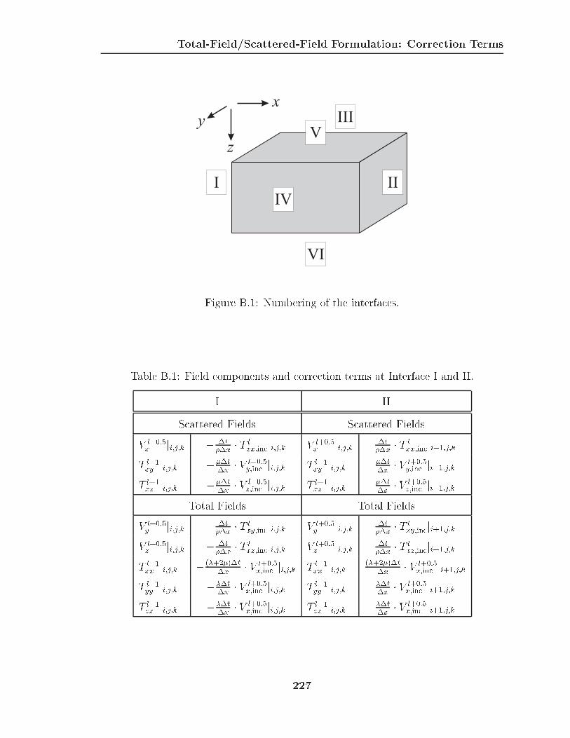
Total-Field/Scattered-Field Formulation: Correction Terms
I II
III
IV
V
VI
x
y
z
Figure B.1: Numbering of the interfaces.
Table B.1: Field components and correction terms at Interface I and II.
I II
Scattered Fields Scattered Fields
V l+0:5x ji;j;k � �t
��x� T l
xx;incji;j;k V l+0:5x ji;j;k �t
��x� T l
xx;incji�1;j;kT l+1xy ji;j;k ���t
�x� V l+0:5
y;inc ji;j;k T l+1xy ji;j;k ��t
�x� V l+0:5
y;inc ji�1;j;kT l+1xz ji;j;k ���t
�x� V l+0:5
z;inc ji;j;k T l+1xz ji;j;k ��t
�x� V l+0:5
z;inc ji�1;j;kTotal Fields Total Fields
V l+0:5y ji;j;k � �t
��x� T l
xy;incji;j;k V l+0:5y ji;j;k �t
��x� T l
xy;incji+1;j;kV l+0:5z ji;j;k � �t
��x� T l
xz;incji;j;k V l+0:5z ji;j;k �t
��x� T l
xz;incji+1;j;kT l+1xx ji;j;k � (�+2�)�t
�x� V l+0:5
x;inc ji;j;k T l+1xx ji;j;k (�+2�)�t
�x� V l+0:5
x;inc ji+1;j;kT l+1yy ji;j;k ���t
�x� V l+0:5
x;inc ji;j;k T l+1yy ji;j;k ��t
�x� V l+0:5
x;inc ji+1;j;kT l+1zz ji;j;k ���t
�x� V l+0:5
x;inc ji;j;k T l+1zz ji;j;k ��t
�x� V l+0:5
x;inc ji+1;j;k
227
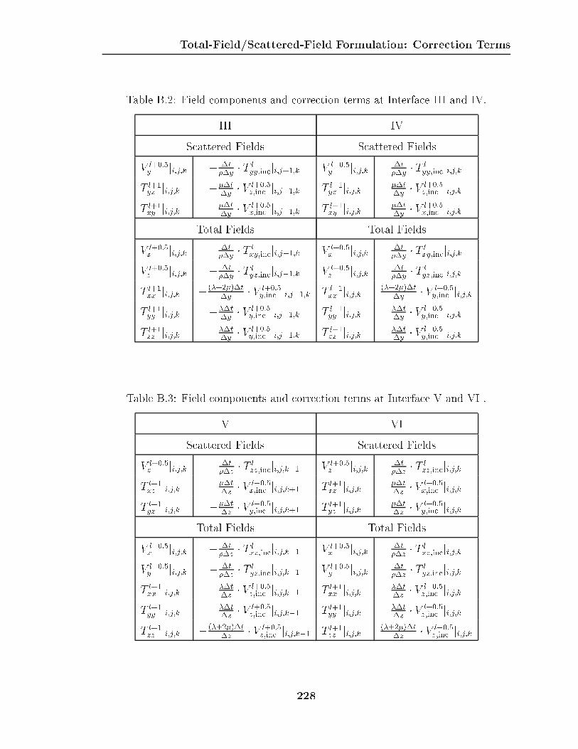
Total-Field/Scattered-Field Formulation: Correction Terms
Table B.2: Field components and correction terms at Interface III and IV.
III IV
Scattered Fields Scattered Fields
V l+0:5y ji;j;k � �t
��y� T l
yy;incji;j+1;k V l+0:5y ji;j;k �t
��y� T l
yy;incji;j;kT l+1yz ji;j;k ���t
�y� V l+0:5
z;inc ji;j+1;k T l+1yz ji;j;k ��t
�y� V l+0:5
z;inc ji;j;kT l+1xy ji;j;k ���t
�y� V l+0:5
x;inc ji;j+1;k T l+1xy ji;j;k ��t
�y� V l+0:5
x;inc ji;j;kTotal Fields Total Fields
V l+0:5x ji;j;k � �t
��y� T l
xy;incji;j�1;k V l+0:5x ji;j;k �t
��y� T l
xy;incji;j;kV l+0:5z ji;j;k � �t
��y� T l
yz;incji;j�1;k V l+0:5z ji;j;k �t
��y� T l
yz;incji;j;kT l+1xx ji;j;k � (�+2�)�t
�y� V l+0:5
y;inc ji;j�1;k T l+1xx ji;j;k (�+2�)�t
�y� V l+0:5
y;inc ji;j;kT l+1yy ji;j;k ���t
�y� V l+0:5
y;inc ji;j�1;k T l+1yy ji;j;k ��t
�y� V l+0:5
y;inc ji;j;kT l+1zz ji;j;k ���t
�y� V l+0:5
y;inc ji;j�1;k T l+1zz ji;j;k ��t
�y� V l+0:5
y;inc ji;j;k
Table B.3: Field components and correction terms at Interface V and VI .
V VI
Scattered Fields Scattered Fields
V l+0:5z ji;j;k � �t
��z� T l
zz;incji;j;k+1 V l+0:5z ji;j;k �t
��z� T l
zz;incji;j;kT l+1xz ji;j;k ���t
�z� V l+0:5
x;inc ji;j;k+1 T l+1xz ji;j;k ��t
�z� V l+0:5
x;inc ji;j;kT l+1yz ji;j;k ���t
�z� V l+0:5
y;inc ji;j;k+1 T l+1yz ji;j;k ��t
�z� V l+0:5
y;inc ji;j;kTotal Fields Total Fields
V l+0:5x ji;j;k � �t
��z� T l
xz;incji;j;k�1 V l+0:5x ji;j;k �t
��z� T l
xz;incji;j;kV l+0:5y ji;j;k � �t
��z� T l
yz;incji;j;k�1 V l+0:5y ji;j;k �t
��z� T l
yz;incji;j;kT l+1xx ji;j;k ���t
�z� V l+0:5
z;inc ji;j;k�1 T l+1xx ji;j;k ��t
�z� V l+0:5
z;inc ji;j;kT l+1yy ji;j;k ���t
�z� V l+0:5
z;inc ji;j;k�1 T l+1yy ji;j;k ��t
�z� V l+0:5
z;inc ji;j;kT l+1zz ji;j;k � (�+2�)�t
�z� V l+0:5
z;inc ji;j;k�1 T l+1zz ji;j;k (�+2�)�t
�z� V l+0:5
z;inc ji;j;k
228
APPENDIX C
Software Documentation
The numerical model has been implemented using FORTRAN90. The three-dimensional
model is written in a fully parallel fashion using the Message-Passing Interface (MPI)
to run on computers with multiple processors. It can be executed on any machine
on which MPI is installed by using the default MPI execution command (mpirun) or a
script �le called execute gui. The script �le requires certain input parameters:
execute gui <np> <machine file> <executable> <directory>
<input file>
<np> speci�es the number of processors that are to be used, <machine file> is a
�le containing a listing of all machines that are to be used (i. e., the names of the
nodes of the parallel computer), <executable> is the program name to be executed,
<directory> is the name (including the path) of the directory in which the output
data is to be stored, and <input file> is the name of the �le in which the program
parameters are speci�ed. For example,
execute gui 28 machines 3d parallel /nodes/data parameters.dat
executes the �le 3d parallel using 28 processors (whose names are speci�ed in
machines), reads in the program parameters from parameters.dat and stores the
output in the directory /nodes/data.
229

C.1 Input File
C.1 Input File
The input parameters are speci�ed in the input �le. The name of the input �le is
arbitrary and must be speci�ed during the program execution. The input �le consists
of �ve sections. In the �rst section, the general simulation parameters are speci�ed.
This section must appear �rst. In the four other sections, sources and objects in
the solution space are speci�ed, the background material is de�ned and the material
properties of the objects are listed. Each section must be started with a characteristic
letter:
� G for 'GENERAL',
� S for 'SOURCE',
� O for 'OBJECT',
� B for 'BACKGROUND', and
� M for 'MATERIAL'.
Each section is ended with the statement END. Comments can be inserted anywhere
and are indicated by either C followed by a space or # at the beginning of the line.
C.1.1 General Simulation Parameters
This section must appear �rst. The section beginning is indicated by G, and the end
by END. The following parameters must be speci�ed or errors will occur:
� DIM = x y zproblem dimensions in x, y and x [cm]
� DISCRETIZATION = dx dy dzsize of space steps �x, �y, �z [cm]
� TIME = ttime [ms]
� FREESURFACE = <0/1>
0: no free surface, 1: free surface at z = 0
230

C.1 Input File
� SYMMETRIE Y = <0/1>
0: symmetry not exploited, 1: solution space symmetric to x-z-plane at y = 0.
Each statement begins with a characteristic phrase (e. g. TIME), followed by an equal
sign. After the equal sign, the value(s) is (are) speci�ed.
The time domain output data is written for entire planes. Up to 50 planes can
be speci�ed. Also, the frequency domain data for up to 1000 single points can be
output.
� SAMPLERATEMOVIE = rrate for writing the output [ms]
� OUTPUT PLANE = P lane Positionplane (X,Y,Z, e. g., X for y-z-plane) and its position [cm].A maximum of 50 output planes can be speci�ed. The data for the �rst speci�edplane is written in the �les `x1.dat', `y1.dat', and `z1.dat'; the data for the secondplane in `x2.dat', `y2.dat', and `z2.dat', and so on.
� OUTPUT POINT = fmin fmax �f x y zfrequency range of the output data (min. freq., max. freq., step freq.) and co-ordinates of the point [cm];A maximum of 1000 output points can be speci�ed. The frequency domain datafor the �rst speci�ed output point is written in `freq x1.dat', `freq y1.dat', and`freq z1.dat'; for the second point in `freq x2.dat', `freq y2.dat', and `freq z2.dat',and so on.
A sample input �le might look like this:
DIM = 30. 30. 30.
DISCRETIZATION = 0.5 0.5 0.5
TIME = 40.
FREESURFACE = 1
SYMMETRIE Y = 1
SAMPLERATEMOVIE = 0.125
OUTPUT PLANE = Z 0.
OUTPUT POINT = 0. 1500. 5. 15. 10. 10.
END
This input produces a solution space of size 30 cm by 30 cm by 30 cm (excluding
PML) with a spacing between the nodes of 0.5 cm in x, y and z. The �elds are
231

C.1 Input File
computed for 40 milliseconds, a free surface boundary is present at z = 0, the �elds
are symmetric to the x-z-plane at y = 0. The output is written for the x-y-plane at
z = 0 (equivalent to the surface plane) with a rate of one frame per 0.125 milliseconds
(equivalent to a sample rate of 8 kHz). The frequency domain data is written out
for the point (x; y; z) = (15 cm; 10 cm; 10 cm) in the range from 0 Hz to 1500 Hz.
Note that all length speci�cations are in centimeters, and all time speci�cations are
in milliseconds.
C.1.2 Sources
Up to 100,000 source points can be speci�ed. Additionally, 10 plane waves (shear or
pressure) can be injected. Note that all length speci�cations are in centimeters, and
all time speci�cations are in milliseconds.
� CENTERFREQUENCY = fcentercenter frequency of excitation [Hz]; must be speci�ed!
� POINT = x y z tdelay iexc D Acoordinates of the point source [cm], time delay [ms], type of excitation (0,1,2),direction (X,Y,Z) and amplitude of excitation
� CIRCLE = xcenter ycenter zcenter d �az �ele tdelay iexc D Acoordinates of the center of the source [cm], diameter [cm], azimuth and eleva-tion angle [degrees], time delay [ms], type of excitation (0,1,2), direction (X,Y,Z)and amplitude of excitation
� SQUARE = xcenter ycenter zcenter xdim ydim �az �ele tdelay iexc D Acoordinates of the center of the source [cm], dimensions in x and y [cm], az-imuth and elevation angle [degrees], time delay [ms], type of excitation (0,1,2),direction (X,Y,Z) and amplitude of excitation
� RING = xcenter ycenter zcenter d w �az �ele tdelay iexc D Acoordinates of the center of the source [cm], diameter and width of the ring[cm], azimuth and elevation angle [degrees], time delay [ms], type of excitation(0,1,2), direction (X,Y,Z) and amplitude of excitation
� CUBE = xcenter ycenter zcenter xdim ydim zdim �az �ele tdelay iexc D Acoordinates of the center of the source [cm], dimensions in x, y and z [cm],azimuth and elevation angle [degrees], time delay [ms], type of excitation (0,1,2),direction (X,Y,Z) and amplitude of excitation
232

C.1 Input File
� SPHERE = xcenter ycenter zcenter d tdelay iexc D Acoordinates of the center of the source [cm], diameter [cm], time delay [ms],type of excitation (0,1,2), direction (X,Y,Z) and amplitude of excitation
� CYLINDER = xcenter ycenter zcenter d zdim �az �ele tdelay iexc D Acoordinates of the center of the source [cm], diameter and height of cylinder[cm], azimuth and elevation angle [degrees], time delay [ms], type of excitation(0,1,2), direction (X,Y,Z) and amplitude of excitation
� SPHERICAL SHELL = xcenter ycenter zcenter d w tdelay iexc D Acoordinates of the center of the source [cm], diameter and width of shell [cm],azimuth and elevation angle [degrees], time delay [ms], type of excitation (0,1,2),direction (X,Y,Z) and amplitude of excitation
� CYLINDRICAL SHELL = xcenter ycenter zcenter d w zdim �az �ele tdelay iexc D Acoordinates of the center of the source [cm], diameter, width and height ofcylinder [cm], azimuth and elevation angle [degrees], time delay [ms], type ofexcitation (0,1,2), direction (X,Y,Z) and amplitude of excitation
� PLANEWAVE = Type Dir tdelay iexc Atype of wave (PRESSURE,SHEAR), propagation direction and polarization (X,Y,Zfor PRESSURE; XZ, ... for SHEAR, indicating a shear wave polarized in x andpropagating in z), time delay [ms], type of excitation (0,1,2) and amplitude ofexcitation
� PRESSURE SOURCE = xcenter ycenter zcenter d w tdelay iexc ASpherical source that emits mainly spherical pressure waves; coordinates ofthe center of the source [cm], diameter of source [cm], width of bu�er layersurrounding the source to suppress shear waves [cm] (recommended: 2.), timedelay [ms], type of excitation (0,1,2) and amplitude of excitation
The azimuth angle is the angle by which the source is to be rotated from the
x-axis towards the y-axis in the x-y-plane.
The elevation angle is the angle by which the source is to be rotated from the
x-axis towards the z-axis in the x-z-plane.
Three types of excitation are possible indicated by 0, 1, and 2:
0 = di�erentiated Gaussian pulse
1 = Gaussian pulse
2 = external data speci�ed in the �le source.dat
233

C.1 Input File
Format of source.dat: the �rst column speci�es the time data, the second column the
excitation values.
C.1.3 Objects
Objects with up to 1,000,000 elements can be speci�ed.
� ROUNDMINE = xref yref zref d1 zdim;1 d2 zdim;2 �az �ele iMat1 iMat2
reference location of mine (center in x and y, top of mine in z) [cm], diame-ter and height of large chamber, diameter and height of small chamber [cm],azimuth and elevation angle [degrees], material indices of large and small cham-ber, respectively
� SQUAREMINE = xref yref zref xdim;1 ydim;1 zdim;1 xdim;2 ydim;2 zdim;2 �az �ele iMat1
iMat2
reference location of mine (center in x and y, top of mine in z) [cm], dimensionsin x, y and z of large chamber, dimensions in x, y and z of small chamber[cm], azimuth and elevation angle [degrees], material indices of large and smallchamber, respectively
� DETAILED TS50 = xref yref zref �az �ele iMat1 iMat2 iMat3 iMat4
reference location of mine (center in x and y, top of mine in z) [cm], azimuthand elevation angle [degrees], material indices of explosives, air, case and rubberplate, respectively
� POINT = xref yref zref iMat
location in x, y and z [cm], material index
� CUBE = xref yref zref xdim ydim zdim �az �ele iMat
reference location of cube (center in x and y, top of object in z) [cm], dimensionsin x, y and z [cm], azimuth and elevation angle [degrees], material index
� SPHERE = xref yref zref d iMat
reference location of sphere (center in x and y, top of object in z) [cm], diameterof sphere [cm], material index
� SPHERICAL SHELL = xref yref zref d w iMat1 iMat2
reference location of shell (center in x and y, top of object in z) [cm], overall
234

C.1 Input File
diameter of shell [cm], width of shell wall [cm], material index of shell wall,material index of inner material
� CYLINDER = xref yref zref d zdim �az �ele iMat
reference location of disk (center in x and y, top of object in z) [cm], diame-ter and height of disk [cm], azimuth and elevation angle [degrees], material index
� CYLINDRICAL SHELL = xref yref zref d zdim w �az �ele iMat;1 iMat;2
reference location of shell (center in x and y, top of object in z) [cm], diameter,height and width of shell [cm], azimuth and elevation angle [degrees], materialindices of the shell and the inside of the shell, respectively
� DISK LOOSESAND = xref yref zref dobj zdim;obj dsand zdim;sand �az �ele iMat1 iMat2
disk buried in medium with di�erent properties than surrounding soil to simu-late burying e�ects; reference location of disk (center in x and y, top of objectin z) [cm], diameter and height of disk [cm], diameter and height of surroundingregion, azimuth and elevation angle of disk [degrees], material indices of diskand surrounding region
� STICK = xref yref zref d l �az �ele iMat
emulates the random shape of a wooden stick, aligned with the x-axis; referencelocation of the stick is the center of the cross section at the front end; referencelocation [cm], diameter and length of stick [cm], azimuth and elevation angle[degrees], material index
� RANDOMROCK = xref yref zref zdim �az �ele iMat
emulates the random shape of a rock; reference location is the center of therock's upper face; reference location [cm], height [cm], azimuth and elevationangle [degrees], material index
� TUNINGFORK = xref yref zref iMat
tuning fork; reference location is the center of the forking point; reference loca-tion [cm], material index
� EXTERNAL = �le iMat
reads in externally speci�ed objects from �le (�le contains three columns spec-ifying the coordinates of the elements in x, y, and z); material index of theelements
235

C.1 Input File
The coordinates of all source and object elements are written into the �le
prop.dat. Format of prop.dat: four columns containing the coordinates in x, y, and
z, and the material index.
C.1.4 Background
Four di�erent background conditions (i. e., properties of the soil) can be speci�ed:
a homogeneous background, a layered background, a linearly varying background,
and a background in which the shear wave speed varies smoothly. The variation is
assumed to be in the z-direction. The background must be speci�ed only once!
� HOMOGENEOUS = � cP cSmaterial density [kg/m3], pressure wave speed and shear wave speed [m/s]
� LAYERED = nd1 �1 cP1 cS1d2 �2 cP2 cS2
...dn �n cPn cSn
Speci�cation of a layered background medium, in which the material propertiesare piecewise constant; n is the number of horizontal layers in the medium,and in subsequent lines the speci�cation of these layers: thickness of layer [cm],material density [kg/m3], pressure wave speed and shear wave speed [m/s]
� LINEAR = nd1 �1;1 �1;2 cP1;1 cP1;2 cS1;1 cS1;2d2 �2;1 �2;2 cP2;1 cP2;2 cS2;1 cS2;2
...dn �n;1 �n;2 cPn;1 cPn;2 cSn;1 cSn;2
Speci�cation of a layered background medium, in which the material propertiesvary linearly; n is the number of horizontal layers in the medium, and in sub-sequent lines the speci�cation of these layers: thickness of layer [cm], materialdensities at upper and lower interface [kg/m3], pressure wave speeds and shearwave speeds at upper and lower interface [m/s]
� DEPTHVARYING = � cP cS;min cS;max A BSpeci�cation of a background medium in which the shear wave speed variessmoothly; material density [kg/m3], pressure wave speed, minimum shear wavespeed, maximum shear wave speed [m/s], and the constants A and B, indicating
236

C.1 Input File
the fraction of the maximum shear wave speed reached at a depth of one meter,and the growth rate, respectively.
The material properties in the soil are written out to the �le background.dat.
Format of background.dat: four columns containing the depth, the material density,
the pressure wave speed and the shear wave speed in the model as a function of depth.
C.1.5 Materials
The materials that are used to characterize the objects must be speci�ed. Only the
materials that are actually used should be speci�ed, because the size of the time step
is determined from the maximum occurring wave speed in the list of the material
speci�cations. The materials are identi�ed by indices. Up to 100 di�erent materials
can be input.
Each material is de�ned by a material index iMat, the density �, the pressure
wave speed cP , and the shear wave speed cS. All of these must be speci�ed. A sample
input �le might look like this:
M
# air
1 1.3 330. 0.
# plastic
2 1200. 2700. 1100. END
Here, the parameters for air and plastic are de�ned. Air has the index 1, a density
of 1.3 kg/m3, a pressure wave speed of 330 m/s and a shear wave speed of 0 m/s.
Plastic has the index 2, a density of 1200 kg/m3, a pressure wave speed of 2700 m/s
and a shear wave speed of 1100 m/s.
C.1.6 Sample Input File
237

C.1 Input File
# Sample Input File
# input general problem parameters
G
DIM = 30.0 30.0 30.0
DISCRETIZATION = 0.5 0.5 0.5
TIME = 30.0
FREESURFACE = 1
SYMMETRIE Y = 1
SAMPLERATEMOVIE = 0.1
OUTPUT PLANE = Z 0.0
OUTPUT PLANE = X 10.0
OUTPUT PLANE = Y 0.0
OUTPUT POINT = 0.0 1500.0 5.0 10.0 10.0 10.0
OUTPUT POINT = 0.0 1500.0 5.0 15.0 10.0 10.0
END
# input sources
S
CENTERFREQUENCY = 450.0
SQUARE = 10.0 0.0 10.0 1.5 10.0 0.0 0.0 5.0 1 X 1.0
END
# input objects
O
ROUNDMINE = 15.0 0.0 3.0 8.0 3.0 4.0 1.0 0.0 0.0 2 1
EXTERNAL = ext.dat 1
END
# input background
B
HOMOGENEOUS = 1400.0 250.0 87.0
END
# define materials
M
# air
1 1.3 330.0 0.0
# plastic
2 1200.0 2700.0 1100.0
END
238

APPENDIX D
Elastic Constants for Isotropic Solids
Pressure Wave Speed in a
Medium:cP =
s�+ 2�
�
Shear Wave Speed in a Medium: cS =
s�
�
Poisson's Ratio: � =0:5�
� + �
Young's Modulus: E =�(3�+ 2�)
�+ �
Longitudinal Wave Speed in a
Plate:cL =
sE
�(1� �2)
Transverse Flexural Wave Speed
in a Plate:cTF =
vuuth!
E
12�(1� �2)
!1=2
239

Bibliography
[1] C. Stewart, \Proposed massless remote vibration pickup," J. Acoust. Soc. Am.,vol. 30, pp. 644{645, 1958.
[2] J. M. Sabatier, H. E. Bass, L. N. Bolen, K. Attenborough, and V. S. Sastry,\The interaction of airborne sound with the porous ground: The theoreticalformulation," J. Acoust. Soc. Am., vol. 79, no. 5, pp. 1345{1352, May 1986.
[3] J. M. Sabatier, H. E. Bass, L. N. Bolen, and K. Attenborough, \Acousticallyinduced seismic waves," J. Acoust. Soc. Am., vol. 80, no. 2, pp. 646{649, Aug.1986.
[4] W. P. Arnott and J. M. Sabatier, \Laser-doppler vibrometer measurements ofacoustic to seismic coupling," Applied Acoustics, vol. 30, pp. 279{291, 1990.
[5] \Feasibility of acoustic landmine detection: Final technical report," Tech. Rep.,BBN Systems and Technologies, Cambridge, MA, 1992.
[6] K. Attenborough, J. M. Sabatier, and C. Frederickson, \The sound �eld withina rigid porous layer," Applied Acoustics, vol. 45, pp. 283{296, 1995.
[7] D. Donskoy, \Nonlinear vibro-acoustic technique for landmine detection," inDetection and Remediation Technologies for Mines and Minelike Targets III,Proc. SPIE, Apr. 1998, vol. 3392, pp. 211{217.
[8] W. R. Scott, Jr., C. T. Schr�oder, and J. S. Martin, \An acousto-electromagneticsensor for locating land mines," in Detection and Remediation Technologies forMines and Minelike Targets III, Proc. SPIE, Apr. 1998, vol. 3392, pp. 176{186.
[9] W. R. Scott, Jr., C. T. Schr�oder, and J. S. Martin, \A hybridacousto/electromagnetic technique for locating land mines," in Proc. Interna-tional Geoscience and Remote Sensing Symposium, Seattle, Wash., Apr. 1998,pp. 216{218.
[10] J. M. Sabatier and N. Xiang, \Acoustic-to-seismic coupling and detection of landmines," in Proc. Geoscience and Remote Sensing Symposium, Jul. 2000, vol. 4,pp. 1646{1648.
240
BIBLIOGRAPHY
[11] J. M. Sabatier and N. Xiang, \An investigation of acoustic-to-seismic couplingto detect buried antitank landmines," IEEE Trans. Geoscience and RemoteSensing, vol. 39, no. 6, pp. 1146{1154, Jun. 2001.
[12] W. R. Scott, Jr., J. S. Martin, and G. D. Larson, \Experimental model for aseismic landmine detection system," IEEE Trans. on Geoscience and RemoteSensing, vol. 39, no. 6, pp. 1155{1164, Jun. 2001.
[13] W. R. Scott, Jr. and J. S. Martin, \Experimental investigation of the acousto-electromagnetic sensor for locating land mines," in Detection and RemediationTechnologies for Mines and Minelike Targets IV, Proc. SPIE, Apr. 1999, vol.3710, pp. 204{214.
[14] W. R. Scott, Jr., G. D. Larson, and J. S. Martin, \Simultaneous use of elasticand electromagnetic waves for the detection of buried land mines," in Detectionand Remediation Technologies for Mines and Minelike Targets V, Proc. SPIE,Apr. 2000, vol. 4038, pp. 667{678.
[15] W. R. Scott, Jr., J. S. Martin, and G. D. Larson, \Investigation of a techniquethat uses elastic waves to detect buried land mines," in Proc. Geoscience andRemote Sensing Symposium, Jul. 2000, vol. 4, pp. 1640{1642.
[16] E. E. Charette, \3D acoustic �nite di�erence on a nCUBE massively parallelcomputer," Tech. Rep., ERL/nCUBE Geophysical Center for Parallel Process-ing, Sep. 1992.
[17] A. Tavlove, Computational Electromagnetics: The Finite-Di�erence Time-Domain Method, Artech House, Boston, 1995.
[18] K. J. Marfurt, \Accuracy of �nite-di�erence and �nite-element modeling of thescalar and elastic wave equations," Geophysics, vol. 49, no. 5, pp. 533{549, May1984.
[19] Z. Alterman and F. C. Karal, Jr., \Propagation of elastic waves in layered mediaby �nite-di�erence methods," Bulletin Seismological Society of America, vol. 58,no. 1, pp. 367{398, Feb. 1968.
[20] M. Ottaviani, \Elastic wave propagation in two evenly-welded quarter-spaces,"Bulletin Seismological Society of America, vol. 61, no. 2, pp. 1119{1152, 1971.
[21] K. R. Kelly, R. W. Ward, S. Treitel, and R. M. Alford, \Synthetic seismograms:a �nite-di�erence approach," Geophysics, vol. 41, no. 1, pp. 2{27, Feb. 1976.
[22] A. Ilan and D. Loewenthal, \Instability of �nite di�erence schemes due to bound-ary conditions in elastic media," Geoph. Prosp., vol. 24, no. 3, pp. 431{453, Sep.1976.
241

BIBLIOGRAPHY
[23] B. Kummer and A. Behle, \Second-order �nite-di�erence modeling of SH-wavepropagation in laterally inhomogeneous media," Bulletin Seismological Societyof America, vol. 72, no. 3, pp. 793{808, Jun. 1982.
[24] S. H. Emerman, W. Schmidt, and R. A. Stephen, \An implicit �nite-di�erenceformulation of the elastic wave equation," Geophysics, vol. 47, no. 11, pp. 1521{1526, Nov. 1982.
[25] R. Madariaga, \Dynamics of an expanding circular fault," Bulletin SeismologicalSociety of America, vol. 66, pp. 639{666, 1976.
[26] J. Virieux, \SH-wave propagation in heterogenous media: Velocity-stress �nite-di�erence method," Geophysics, vol. 49, no. 11, pp. 1933{1957, Nov. 1984.
[27] J. Virieux, \P-SV wave propagation in heterogenous media: Velocity-stress�nite-di�erence method," Geophysics, vol. 51, no. 4, pp. 889{901, Apr. 1986.
[28] K. S. Yee, \Numerical solution of initial boundary value problems involvingMaxwell's equations in isotropic media," IEEE Trans. Antennas Propagat., vol.14, pp. 302{307, 1966.
[29] A. R. Levander, \Fourth-order �nite-di�erence P-SV seismograms," Geophysics,vol. 51, no. 11, pp. 1424{1436, Nov. 1988.
[30] N. Dai, A. Vai�dis, and E. R. Kanasewich, \Wave propagation in heterogeneous,porous media: a velocity-stress, �nite-di�erence method," Geophysics, vol. 60,no. 2, pp. 327{340, Apr. 1995.
[31] Y. Q. Zeng and Q.-H. Liu, \Acoustic detection of buried objects in 3-D uidsaturated porous media: Numerical modeling," IEEE Trans. Geoscience andRemote Sensing, vol. 39, no. 6, pp. 1165{1173, Jun. 2001.
[32] B. K. Sinha, Q.-H. Liu, and S. Kostek, \Acoustic waves in pressurized boreholes:a �nite-di�erence formulation," J. Geophysical Research, vol. 101, no. B11, pp.25,173{25,180, Nov. 1996.
[33] T. D. Mast, L. M. Hinkelman, L. A. Metlay, M. J. Orr, and R. C. Waag, \Sim-ulation of ultrasonic pulse propagtion, distortion, and attenuation in the humanchest wall," J. Acoust. Soc. Am., vol. 106, no. 6, pp. 3665{3677, Jun. 2001.
[34] E. S. Krebes and G. Quiroga-Goode, \A standard �nite-di�erence scheme forthe time-domain computation of anelastic wave�elds," Geophysics, vol. 59, no.2, pp. 290{296, Feb. 1994.
[35] J. O. A. Robertson, J. O. Blanch, and W. W. Symes, \Viscoelastic �nite-di�erence modeling," Geophysics, vol. 59, no. 9, pp. 1444{1456, Sep. 1994.
242

BIBLIOGRAPHY
[36] E. L. Faria and P. L. Sto�a, \Finite-di�erence modeling in transversely isotropicmedia," Geophysics, vol. 59, no. 2, pp. 282{289, Feb. 1994.
[37] M. A. Biot, \Theory of propagation of elastic waves in a uid-saturated poroussolid. I. low-frequency range," J. Acoust. Soc. Am., vol. 28, no. 2, pp. 168{178,Mar. 1956.
[38] J. E. Vidale and R. W. Clayton, \A stable free-surface boundary condition fortwo-dimensional elastic �nite-di�erence wave simulation," Geophysics, vol. 51,no. 12, pp. 2247{2249, Dec. 1986.
[39] R. Clayton and B. Engquist, \Absorbing boundary conditions for acoustic andelastic wave equations," Bulletin Seismological Society of America, vol. 67, no.6, pp. 1529{1540, Dec. 1977.
[40] S. H. Emerman and R. A. Stephen, \Comment on 'Absorbing boundary condi-tions for acoustic and elastic wave equations'," Bulletin Seismological Society ofAmerica, vol. 73, no. 2, pp. 661{665, Apr. 1983.
[41] K. D. Mahrer, \Numerical time step instability and Stacey's andClayton-Engquist's absorbing boundary conditions," Bulletin Seismological So-ciety of America, vol. 80, no. 1, pp. 213{217, Feb. 1990.
[42] R. G. Keys, \Absorbing boundary conditions for acoustic media," Geophysics,vol. 50, no. 6, pp. 892{902, Jun. 1985.
[43] C. J. Randall, \Absorbing boundary condition for the elastic wave equation,"Geophysics, vol. 53, no. 5, pp. 611{624, May 1988.
[44] W.-F. Chang and G. A. McMechan, \Absorbing boundary conditions for 3-Dacoustic and elastic �nite-di�erence calculations," Bulletin Seismological Societyof America, vol. 79, no. 1, pp. 211{218, Feb. 1989.
[45] R. A. Renault and J. Petersen, \Stability of wide-angle absorbing boundaryconditions for the wave equation," Geophysics, vol. 54, no. 9, pp. 1153{1163,Sep. 1989.
[46] C. J. Randall, \Absorbing boundary condition for the elastic wave equation:Velocity-stress formulation," Geophysics, vol. 54, no. 9, pp. 1141{1152, Sep.1989.
[47] L. T. Long and J. S. Liow, \A transparent boundary for �nite-di�erence wavesimulation," Geophysics, vol. 55, no. 2, pp. 201{208, Feb. 1990.
[48] C. Peng and M. N. Toksoez, \An optimal absorbing boundary condition for�nite-di�erence modeling of acoustic and elastic wave propagation," J. Acoust.Soc. Am., vol. 95, no. 2, pp. 733{745, Feb. 1994.
243

BIBLIOGRAPHY
[49] J.-P. Berenger, \A perfectly matched layer for the absorption of electromagneticwaves," J. Comput. Physics, vol. 114, pp. 185{200, 1994.
[50] Z. S. Sacks, D. M. Kingsland, R. Lee, and J. F. Lee, \A perfectly matchedanisotropic absorber for use as an absorbing boundary condition," IEEE Trans.Antennas Propagat., vol. 43, pp. 1460{1463, Dec. 1995.
[51] S. D. Gedney, \An anisotropic perfectly matched layer-absorbing medium forthe truncation of FDTD-Lattices," IEEE Trans. Antennas Propagat., vol. 44,pp. 1630{1639, Dec. 1996.
[52] L. Zhao and A. C. Cangellaris, \GT-PML: generalized theory of perfectlymatched layers and its application to the re ectionless truncation of �nite-di�erence time-domain grids," IEEE Trans. Microwave Theory and Techniques,vol. 44, no. 12, pp. 2555{2563, Dec. 1996.
[53] J.-P. Berenger, \Improved PML for the FDTD solution of wave-structure inter-action problems," IEEE Trans. Antennas Propagat., vol. 45, pp. 466{473, Mar.1997.
[54] F. D. Hastings, J. B. Schneider, and S. L. Broschat, \Application of the per-fectly matched layer (PML) absorbing boundary condition to elastic wave prop-agation," J. Acoust. Soc. Am., vol. 100, no. 5, pp. 3061{3068, Nov. 1996.
[55] W. C. Chew and Q. H. Liu, \Perfectly matched layer for elastodynamics; a newabsorbing boundary condition," J. Comput. Acoustics, vol. 4, pp. 341{359, 1996.
[56] X. Yuan, D. Borup, J. W. Wiskin, M. Berggren, R. Eidens, and S. A. John-son, \Formulation and validation of Berenger's PML absorbing boundary forthe FDTD simulation of acoustic scattering," IEEE Trans. Ultrasonics, Ferro-electrics, Frequency Control, vol. 44, no. 4, pp. 816{822, Jul. 1997.
[57] B. A. Auld, Acoustic Fields and Waves in Solids, vol. 1 and 2, Robert E. KriegerPublishing Company, 2nd edition, 1990.
[58] K. F. Gra�, Wave Motion in Elastic Solids, Dover Publications, 1975.
[59] A. Tavlove, Advances in Computational Electromagnetics: The Finite-Di�erenceTime-Domain Method, Artech House, Boston, 1998.
[60] http://www.beowulf.org.
[61] R. D. Richtmyer, Di�erence Methods for Initial Value Problems, John Wileyand Sons, New York, 2nd edition, 1967.
[62] G. D. Smith, Numerical Solution of Partial Di�erential Equations; Finite Dif-ference Methods, Clarendon Press, 2nd edition, 1978.
244
BIBLIOGRAPHY
[63] A. R. Mitchell and D. F. GriÆths, The Finite Di�erence Method in PartialDi�erential Equations, John Wiley and Sons, New York, 1980.
[64] P. Fox, \The solution of hyperbolic partial di�erential equations by di�erencemethods," in Mathematical Methods for Digital Computers. A. Ralston and H.S.Wilf, Editors, Ch. 16, Wiley, New York, 1964.
[65] D. S. Watkins, Fundamentals of Matrix Computations, John Wiley and Sons,New York, 1991.
[66] J. W. S. Rayleigh, \On waves propagated along the plane surface of an elasticsolid," Proc. Lond. math. Soc., vol. 17, no. 2, pp. 4{11, 1887.
[67] M. Roth, R. Spitzer, and F. Nitsche, \Seismic survey across an environment withvery high Poisson's ratio," in Proc. 12th Annu. Int. Meeting, Symp. Applicationof Geophysics to Engineering and Environmental Problems, 1999, pp. 49{55.
[68] E. Smith, P. S. Wilson, F. W. Bacon, J. F. Manning, J. A. Behrens, and T. G.Muir, \Measurements and localization of interface wave re ections from a buriedtarget," J. Acoust. Soc. Am., vol. 103, no. 5, pp. 2333{2343, May 1998.
[69] N. E. Glass and A. A. Maradudin, \Leaky surface-elastic waves on both at andstrongly corrugated surfaces for isotropic, nondissipative media," J. Appl. Phys.,vol. 54, no. 2, pp. 796{805, Feb. 1983.
[70] G. F. Miller and H. Pursey, \The �eld and radiation impedance of mechanicalradiators on the free surface of a semi-in�nite isotropic solid," Proc. R. Soc., vol.A 223, pp. 521{541, 1954.
[71] J. Miklowitz, The Theory of Elastic Waves and Wave Guides, North-HollandPublishing Company, 1978.
[72] J. D. Achenbach, Wave Propagation in Elastic Solids, North-Holland PublishingCompany, 1973.
[73] L. B. Felsen and N. Marcuvitz, Radiation and Scattering of Waves, IEEE Press,1994.
[74] M. Abramowitz and I. A. Stegun, Handbook of Mathematical Functions, DoverPublications, 9th edition, 1970.
[75] G. B. Arfken and H. J. Weber, Mathematical Methods for Physicists, AcademicPress, 4th edition, 1995.
[76] G. S. Smith, Classical Electromagnetic Radiation, Cambridge University Press,1997.
245

BIBLIOGRAPHY
[77] A. Behboodian, W. R. Scott, Jr., and J. H. McLellan, \Signal processing of elas-tic surface waves for localizing buried land mines," in Proc. 33rd AssilomarConference on Signals, Systems, and Computers, Oct. 1999.
[78] W. R. Scott, Jr., C. T. Schr�oder, G. D. Larson, and J. S. Martin, \Use of elasticwaves for the detection of buried land mines," in Proc. IGARSS, Jul. 2001.
[79] N. H. Fletcher and T. D. Rossing, The Physics of Musical Instruments, Springer-Verlag, New York, 1st edition, 1991.
[80] T. D. Rossing, D. A. Russell, and David E. Brown, \On the acoustics of tuningforks," Am. J. Phys., vol. 60, no. 6, pp. 620{626, Jul. 1992.
[81] M. W. Sprague, R. Raspet, H. E. Bass, and J. M. Sabatier, \Low frequencyacoustic ground impedance measurement technique," Applied Acoustics, vol. 39,pp. 307{325, 1993.
[82] B. M. Das, Principles of Soil Dynamics, PWS-Kent Publishing Company,Boston, 1993.
[83] R. Bachrach and A. Nur, \High-resolution shallow seismic experiments in sand,"Geophysics, vol. 63, no. 4, pp. 1225{1240, Jul. 1998.
[84] A. V. Oppenheim and R. W. Schafer, Discrete-Time Signal Processing, PrenticeHall, 1989.
[85] C. T. Schr�oder and W. R. Scott, Jr., \Finite-di�erence time-domain model forelastic waves in the ground," in Detection and Remediation Technologies forMines and Minelike Targets IV, Proc. SPIE, Apr. 1999, vol. 3710, pp. 1361{1372.
[86] C. T. Schr�oder, A Finite-Di�erence Model for Elastic Waves in the Ground,Diploma Thesis, Technische Universit�at Braunschweig, Jun. 1999.
[87] C. T. Schr�oder and W. R. Scott, Jr., \Three-dimensional FDTD model to studythe elastic-wave interaction with buried land mines," in Detection and Reme-diation Technologies for Mines and Minelike Targets V, Proc. SPIE, Apr. 2000,vol. 4038, pp. 680{690.
[88] C. T. Schr�oder, K. Kim, and W. R. Scott, Jr., \A FDTD model for the interac-tion of elastic waves with buried land mines," J. Acoust. Soc. Am., vol. 107, no.5, Pt. II, pp. 2897, May 2000.
[89] C. T. Schr�oder and W. R. Scott, Jr., \A three-dimensional �nite-di�erencemodel for the interaction of elastic waves with buried land mines," in Proc.Geoscience and Remote Sensing Symposium, Jul. 2000, vol. 1, pp. 26{28.
246

BIBLIOGRAPHY
[90] C. T. Schr�oder and W. R. Scott, Jr., \Resonance behavior of buried land mines,"in Detection and Remediation Technologies for Mines and Minelike Targets VI,Proc. SPIE, Apr. 2001, vol. 4394.
[91] W. R. Scott, Jr., C. T. Schr�oder, and J. S. Martin, \An acousto-electromagneticmethod for detecting buried objects," in Proc.XXVIth General Assembly of theInternational Union of Radio Science, Toronto, Canada, Aug. 1999, vol. 3710,p. 724.
[92] W. R. Scott, Jr., C. T. Schr�oder, J. S. Martin, and G. D. Larson, \Investiga-tion of a technique that uses both elastic and electromagnetic waves to detectburied land mines," in Proc. AP2000 - Millennium Conference an Antennas andPropagation, Davos, Switzerland, Apr. 2000.
[93] C. T. Schr�oder and W. R. Scott, Jr., \A �nite-di�erence model to study theelastic-wave interactions with buried land mines," IEEE Trans. on Geoscienceand Remote Sensing, vol. 38, pp. 1505{1512, Jul. 2000.
[94] C. T. Schr�oder and W. R. Scott, Jr., \Elastic waves interacting with buriedland mines: a study using the FDTD method," submitted to the IEEE Trans.on Geoscience and Remote Sensing.
[95] C. T. Schr�oder and W. R. Scott, Jr., \On the stability of the FDTD algorithmfor elastic media at a material interface," submitted to the IEEE Trans. onGeoscience and Remote Sensing.
[96] C. T. Schr�oder and W. R. Scott, Jr., \On the complex conjugate roots of therayleigh equation: the leaky surface wave," submitted to the J. Acoust. Soc. Am.
247

VITA
Christoph T. Schr�oder was born in Bonn, Germany, in 1973. He received the M.S.
degree in electrical and computer engineering at the Georgia Institute of Technology,
Atlanta, GA (USA), in 1997, the Diplom der Elektrotechnik from the Technical Uni-
versity of Braunschweig (Germany) in 1999, and the Ph.D. degree in electrical and
computer engineering at the Georgia Institute of Technology in 2001. His research
interests include general wave propagation, remote sensing, numerical modeling in
elasticity and electromagnetics, and the �nite-di�erence time-domain technique.
248