Embed Size (px)
Citation preview
1
UNIVERSITÀ DI PISA
FACOLTÀ DI INGEGNERIA
Corso di Laurea Magistrale in
Ingegneria Biomedica
Tesi di Laurea
Optical filter simulating foveated vision:
modeling and preliminary experiments
Relatori:
Prof. D. De Rossi
Ing. F. Carpi
Candidata:
Eleonora Cipolli
A.A. 2012/2013

2
Alla mia famiglia che mi ha
sostenuta in ogni aspetto fin qui.
A Ramy che mi ha pazientemente
aspettata in questo lungo
cammino.

3
Table of contents
1 INTRODUCTION ................................................................................................................................ 5
2 THE HUMAN EYE AND THE VISUAL PERCEPTION .................................................................. 7
Introduction ........................................................................................................................................ 7
2.1 Anatomy of the eye ....................................................................................................................... 8
2.2 The retina .................................................................................................................................... 11
2.2.1 Structure of the retina ........................................................................................................... 12
2.2.2 Blood supply to the retina .................................................................................................... 14
2.2.3 Fovea structure ..................................................................................................................... 15
2.2.4 Macula lutea ........................................................................................................................ 17
2.2.5 Ganglion cell fiber layer ....................................................................................................... 17
2.2.6 Photoreceptors ...................................................................................................................... 18
2.2.7 Optic nerve ........................................................................................................................... 20
2.3 A review of artificial vision .......................................................................................................... 21
2.3.1Physical approaches .............................................................................................................. 21
2.3.2 Computable methods .......................................................................................................... 23
References ......................................................................................................................................... 26
3 LIGHT SCATTERING ...................................................................................................................... 28
3.1 Introduction to light ................................................................................................................... 28
3.2 Maxwell’s Equations ................................................................................................................... 31
3. 3 Particle theory of light ............................................................................................................... 33
3.4 Quantum theory .......................................................................................................................... 35
3.5 Wave propagation ...................................................................................................................... 36
3. 6 Interaction of electromagnetic radiation and matter ............................................................... 39
3.7 Scattering ................................................................................................................................... 41
3.7.1 Light scattering .................................................................................................................... 44
3.7.2 Types of scattering .............................................................................................................. 45
3.7.3 Rayleigh scattering ............................................................................................................... 45
3.7.4 Mie scattering ...................................................................................................................... 47
3.7.5 Brillouin scattering ............................................................................................................... 47
3.7.6 Raman scattering ................................................................................................................. 47
3.8 Scattering by particles ................................................................................................................ 48

4
3.8.1 Angle- dependent scattering ................................................................................................ 53
References ......................................................................................................................................... 58
4 TUNEABLE OPTICAL FILTER: PROPOSED EVALUATION SYSTEM .................................... 59
4.1 System description ..................................................................................................................... 60
4.2 Electroactive membrane ............................................................................................................ 63
4.3 Filters .......................................................................................................................................... 66
4.4 Frames ......................................................................................................................................... 67
4.5 Housing ........................................................................................................................................ 67
4.6 Camera ........................................................................................................................................ 69
4.7 Optotune Lens ............................................................................................................................. 69
References: ........................................................................................................................................ 71
5 SIMULATION: CST STUDIO SUITE® AND COMSOL MULTIPHYSICS
® ................................. 73
5.1 CST STUDIO SUITE ® ..................................................................................................................... 73
5.1.1 Develop a simulation with CST STUDIO SUITE® ............................................................. 74
5.2 Comsol Multiphysics ® ................................................................................................................. 78
5.2.1 Develop a simulation with Comsol Multiphysics® .............................................................. 79
6 PROTOTYPING: METHODS AND MATERIALS ......................................................................... 81
6.1 Filter ............................................................................................................................................ 81
6.2 Filter characterization ................................................................................................................. 88
6.3 Resolution measurement in Matlab ........................................................................................... 90
References: ........................................................................................................................................ 91
7 RESULTS AND DISCUSSION ........................................................................................................ 92
7.1 Comsol Multiphysics ® results ..................................................................................................... 92
7.2 CST STUDIO SUITE® results .......................................................................................................... 96
7.3 Experimental evaluation: resolution measurement in Matlab ................................................ 104
7.4 Discussion of results .................................................................................................................. 107
8 CONCLUSION AND FUTURE WORK ......................................................................................... 109
APPENDIX ......................................................................................................................................... 110
5
Chapter 1
INTRODUCTION
This thesis is a preliminary work to design an electrically tuneable optical filter based on light
scattering (within the visible spectrum of wavelengths 400 - 700 nm) in order to mimic the foveal
vision in human eyes.
The human vision system is highly dependent on the spatial frequency in sampling, coding, processing
and understanding of how physical due to non-uniformity in the distribution of photoreceptors and
neural cells on the retina.
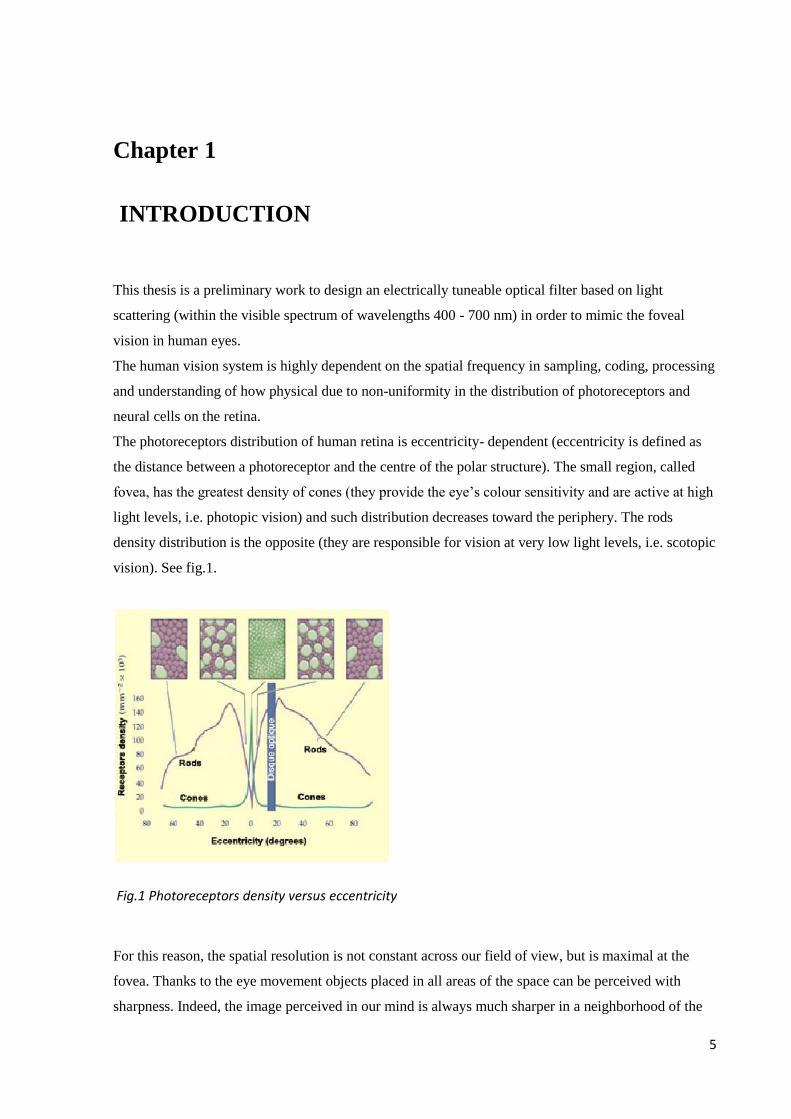
The photoreceptors distribution of human retina is eccentricity- dependent (eccentricity is defined as
the distance between a photoreceptor and the centre of the polar structure). The small region, called
fovea, has the greatest density of cones (they provide the eye’s colour sensitivity and are active at high
light levels, i.e. photopic vision) and such distribution decreases toward the periphery. The rods
density distribution is the opposite (they are responsible for vision at very low light levels, i.e. scotopic
vision). See fig.1.
For this reason, the spatial resolution is not constant across our field of view, but is maximal at the
fovea. Thanks to the eye movement objects placed in all areas of the space can be perceived with
sharpness. Indeed, the image perceived in our mind is always much sharper in a neighborhood of the
Fig.1 Photoreceptors density versus eccentricity
6
gaze point and appears blurred in the surrounding area. For the physical and photochemical features
of rods and cones, the human vision acuity is high (about 60 cyc/ º ) in the fovea. Such a value is about
10 times lower in the periphery.
Several devices or computational solutions have been proposed for mimicking such effect. For
instance Sandini [1] proposed a silicon retina-like sensor characterized by a spatial-variant resolution.
They used a CMOS technology with a log-polar distribution of sensor size.
Other approaches reproduce the foveated vision (FV) using traditional CCD or CMOS sensors with
uniform pixel dimension and applying algorithms through digital filtering, to reduce the effective
resolution in the peripheral part of the image.
On one hand the silicon retinal-like sensor is task-specific and the spatial-variant resolution is fixed
when designed, on the other hand digital filtering increases the computational load of the processing
system and does not take into account to the aliasing problem. In other words sampling targets with
unknown spatial frequency could lead to erroneous data interpretation.
Differently we are looking for a tuneable optical response upon an electrical stimulation so as to
achieve an eccentricity-dependent resolution.
Our work is aimed at developing an optical filter that can be coupled to common CCD or CMOS
sensors. This should be at the same time tuneable, upon an electrically stimulus, and attenuate spatial
frequencies before the photodetector sampling. Our approach is based on the phenomenon of light
scattering to filter the input light signal. We used nano-particles, selected based on size and optical
properties, to create diffusion of light and thus reduce the optical resolution of an image (captured by a
camera- sensor ).The filter should show a spatial variant distribution of the nano-particles, higher in
pheriphery and lower in the centre.
During next chapters the work performer during this thesis is shown. It can be summarized as follow:
- Selection of particles, in terms of sizes and optical properties, based on visible light wavelength.
- Simulation of scattering implemented by the filter (CST STUDIO SUITE® and Comsol
Multiphysics)
- Filter realization where different methods had been tested. This phase concluded with the use of a
flexible substrate to encapsulate nano-particles. The filter obtained has a constant volumetric density
of particles in Sylgard184®
which can be deformed during the activation phase of the electroactive
membrane.
- Resolution measurement in order to evaluate the scattering performed by the filter (in Matlab, with
“sfrmat3” code).
References:
[1] "A retina-like CMOS sensor and its applications." Sandini, Giulio, et al. Sensor Array and
Multichannel Signal Processing Workshop. 2000. Proceedings of the 2000 IEEE. IEEE, 2000
7
Chapter 2
THE HUMAN EYE AND THE VISUAL PERCEPTION
In this chapter we give a brief description of the human visual system describing the anatomy and
physiology of the main structures of the human eye. We will discuss how the human eye is done,
mainly by dwelling on the retina and its photoreceptors, the light-sensitive cells which are responsible
for detecting light and, therefore, enable us to see. The transduction (conversion) of light into nerve
signals that the brain can understand takes place in these specialized cells. They allow us to turn a
scanned image from the optical components of the eye ( cornea and lens ) into an electrical signal and
then convert it back to image inside our brain.
In addition to natural vision , we will present some approaches currently in use that try to mimic the
foveal vision. These techniques can be classified into computationals and physicals ones. We will
present the solutions proposed in literature pointing out the pros and cons of each, thus offering our
work as a additional alternative to bio- engineering systems proposed so far .
Introduction
The human eye is an amazingly complex structure that enables sight, one of the most important of the
human senses. Sight underlies our ability to understand the world around us and to navigate within our
environment. As we look at the world around us, our eyes are constantly taking in light, a component
fundamental to the visual process. The front of the human eye contains a curved lens, through which
light refl ected from objects in the surrounding environment passes. The light travels deep into the
eyeball, passing all the way to the back of the eye, where it converges to a point. A unique set of cells
at the back of the eye receives the light, harnessing its energy by converting it into an electrical
impulse, or signal, that then travels along neurons in the brain. The impulses are carried along a
neuronal pathway that extends from the back of the eye all the way to the back of the brain, ultimately
terminating in a region known as the visual cortex. There, the electrical signals from both eyes are
processed and unified into a single image. The amount of time between the moment when light enters
the eye and when a unified image is generated in the brain is near instantaneous, taking only fractions
of a second.[1]
8
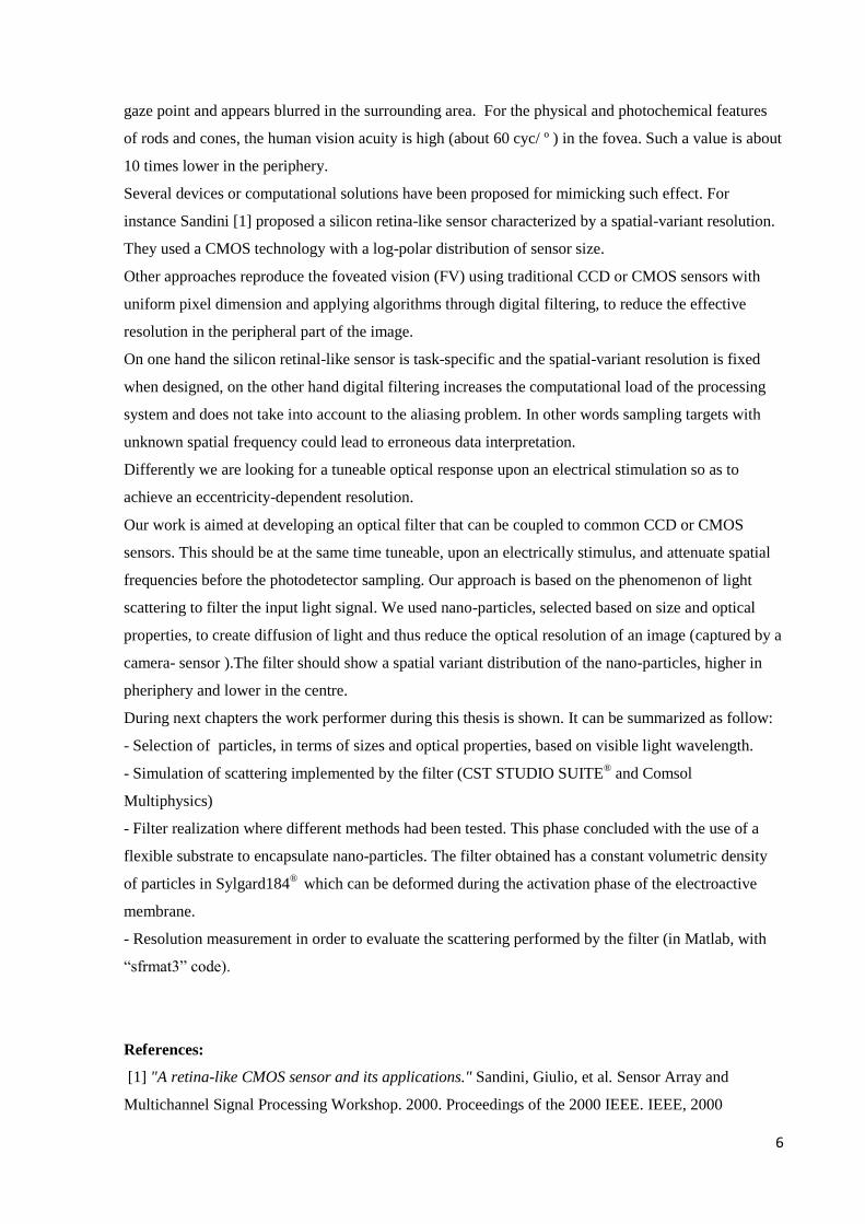
2.1 Anatomy of the eye
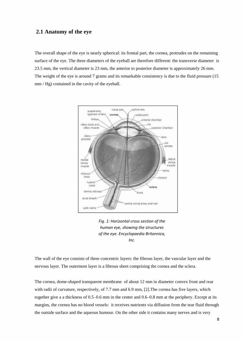
The overall shape of the eye is nearly spherical: its frontal part, the cornea, protrudes on the remaining
surface of the eye. The three diameters of the eyeball are therefore different: the transverse diameter is
23.5 mm, the vertical diameter is 23 mm, the anterior to posterior diameter is approximately 26 mm.
The weight of the eye is around 7 grams and its remarkable consistency is due to the fluid pressure (15
mm / Hg) contained in the cavity of the eyeball.
The wall of the eye consists of three concentric layers: the fibrous layer, the vascular layer and the
nervous layer. The outermost layer is a fibrous sheet comprising the cornea and the sclera.
The cornea, dome-shaped transparent membrane of about 12 mm in diameter convex front and rear
with radii of curvature, respectively, of 7.7 mm and 6.9 mm, [2].The cornea has five layers, which
together give a a thickness of 0.5–0.6 mm in the center and 0.6–0.8 mm at the periphery. Except at its
margins, the cornea has no blood vessels: it receives nutrients via diffusion from the tear fluid through
the outside surface and the aqueous humour. On the other side it contains many nerves and is very
Fig. 1: Horizontal cross section of the
human eye, showing the structures
of the eye. Encyclopaedia Britannica,
Inc.

9
sensitive to pain or touch. It protects the pupil, the iris, and the inside of the eye from penetration by
foreign bodies and it is the first and most powerful element in the eye’s focusing system. As light
passes through the cornea, it is partially refracted before reaching the lens [3]. The cornea has a
refractive index equal to 1.376 and determines most of the refractive power of the eye (approximately
43 dioptres) even if it contributes in a static manner.
The sclera, known as the "white of the eye", forms the supporting wall of the eyeball offering
resistance to internal and external forces thanks to the vitreous humor. It is essentially continuous with
the clear cornea: the collagen fibers of the sclera are an extension of cornea fibers.
The intermediate layer, called vascular tunic or uvea coat, is a vascular layer which consists of the iris,
the choroid, and the ciliary body.
The iris is the pigmented muscular curtain near the front of the eye, between the cornea and the lens,
that is perforated by an opening called the pupil. The iris consists of two sheets of smooth muscle with
contrary actions: dilation (expansion) and contraction (constriction). These muscles control the size of
the pupil and thus determine how much light reaches the sensory tissue of the retina. The sphincter
muscle of the iris is a circular muscle that constricts the pupil in bright light, whereas the dilator
muscle of the iris expands the opening when it contracts. [4] The amount of pigment contained in the
iris determines eye colour.
The average size of the pupil is 3-4 mm : at its maximum contraction, it may be less than 1 mm in
diameter, and it may increase up to 10 times to its maximum diameter. [5]
The choroid, also known as the choroidea or choroid coat, is the vascular layer of the eye,
containing connective tissue, and lying between the retina and the sclera.
The ciliary body is the circumferential tissue inside the eye composed of the ciliary muscle and ciliary
processes [6]It is located behind the iris and before wing choroid. It is triangular in horizontal section
and is coated by a double layer, the ciliary epithelium.
The ciliary body has three functions: accommodation, aqueous humor production and the production,
and maintenance of the lens zonules. It also anchors the lens in place. Accommodation essentially
means that when the ciliary muscle contracts, the lens becomes more convex, generally improving the
focus for closer objects. When it relaxes it flattens the lens, generally improving the focus for farther
objects. One of the essential roles of the ciliary body is also the production of the aqueous humor,
which is responsible for providing most of the nutrients for the lens and the cornea and involved in
waste management of these areas.
The retina is a light-sensitive layer of tissue, at the back of the eye that covers about 65% of its interior
surface. The optics of the eye create an image of the visual world on the retina (through the cornea and
lens) , which serves much the same function as the film in a camera. Light striking the retina initiates a
cascade of chemical and electrical events that ultimately trigger nerve impulses. These are sent to
various visual centres of the brain through the fibres of the optic nerve.
10
The eye can also be divided into two segments, the front and rear. The anterior segment is formed by
the front chamber and the rear which are separated by the iris. Both rooms are filled by 'aqueous
humor, which is a liquid similar to blood plasma actively secreted by the ciliary processes. Its role is to
provide nourishment for the lens and the cornea, to dispose of waste products and to maintain the
shape of the anterior portion of the eye.
The balance between aqueous humor secretion and reabsorption is important to maintain proper
intraocular pressure.
The posterior segment contains instead the vitreous body or vitreous humor which is a colorless and
transparent gelatinous substance that allows the passage of light and also has support function to keep
the shape of the bulb. The two segments are separated by the crystalline lens.
The crystalline lens is a nearly transparent biconvex structure suspended behind the iris of the eye.
Along with the cornea helps to refract light to be focused on the retina.
The lens is made up of unusual elongated cells that have no blood supply but obtain nutrients from the
surrounding fluids, mainly the aqueous humour that bathes the front of the lens. The shape of the lens
can be altered by the relaxation and contraction of the ciliary muscles surrounding it, thus enabling the
eye to focus clearly on objects at widely varying distances. The ability of the lens to adjust from a
distant to a near focus, called accommodation, gradually declines with age.[7]
When the ciliary muscles are relaxed, the tension exerted by the suspensory ligaments tends to flatten
the lens; resting its front surface has a radius of curvature of 10.6 mm and the rear of -6 mm[8].
When the ciliary muscles contract, it reduces the tension of the suspensory ligaments and,
consequently, the lens tends to assume a spheroidal form by virtue of its elastic properties. In the state
of complete accommodation (maximum contraction of the ciliary muscles) the front and rear surfaces
of the lens have a curvature respectively of 6 mm and -5.5 mm [9].
In this state, the dioptric power is maximum and a normal eye can put focus at distances of 25-30 cm
(near point)[10].
The change in dioptric power from the crystal is about 10 diopters, but this value decreases with age.

11
Cornea, aqueous humor, crystalline lens and vitreous body constitute the dioptric means (or dioptric
system or apparatus) of the eye, which can be considered as a converging lens with a significant
refractive power: about 60 diopters.
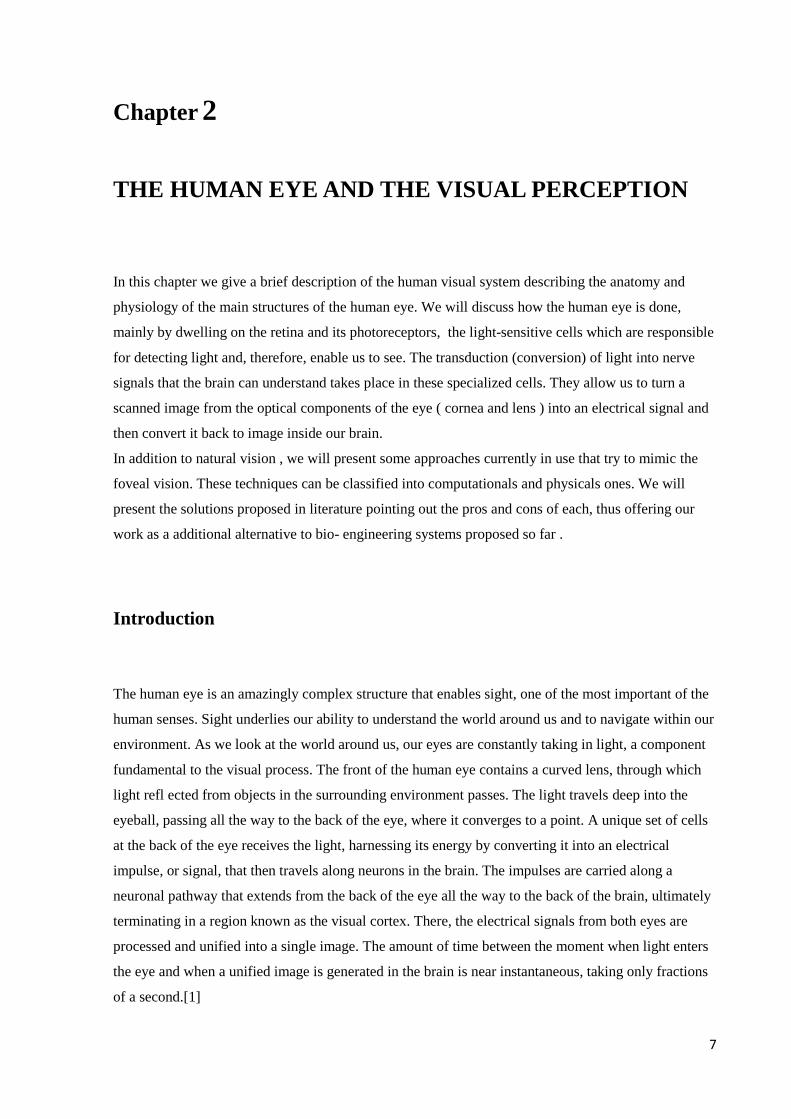
2.2 The retina
The retina is a light-sensitive layer of tissue, lining the inner surface of the eye. When an
ophthalmologist uses an ophthalmoscope to look into your eye he sees the following view of the retina
(Fig. 3).
Fig. 2: Unaccommodated crystalline
lens (A) and accommodate crystalline
lens (B).
Fig. 3: A view of the retina seen
though an ophthalmoscope.
12
In the retina, there are three sections: anterior (retina or iris), average (retina or ciliary) and rear (or
part of the retina or optic retina only). The anterior and middle portions are not able to perceive visual
stimuli, while the rear portion is fully developed and functionally efficient.
The optic disc, a part of the retina sometimes called "the blind spot" because it lacks photoreceptors, is
located at the optic papilla, a nasal zone where the optic-nerve fibers leave the eye. It appears as an
oval white area of 3mm. Most of the vessels of the retina radiate from the center of the optic nerve. In
general, the retina is similar to a circular disc of diameter between 30 and 40 mm and a thickness of
approximately 0.5 mm. The retina is the back part of the eye that contains the cells that respond to
light. These specialized cells are called photoreceptors.
2.2.1 Structure of the retina
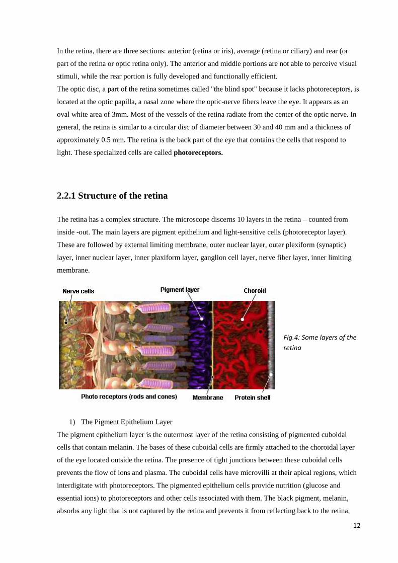
The retina has a complex structure. The microscope discerns 10 layers in the retina – counted from
inside -out. The main layers are pigment epithelium and light-sensitive cells (photoreceptor layer).
These are followed by external limiting membrane, outer nuclear layer, outer plexiform (synaptic)
layer, inner nuclear layer, inner plaxiform layer, ganglion cell layer, nerve fiber layer, inner limiting
membrane.
1) The Pigment Epithelium Layer
The pigment epithelium layer is the outermost layer of the retina consisting of pigmented cuboidal
cells that contain melanin. The bases of these cuboidal cells are firmly attached to the choroidal layer
of the eye located outside the retina. The presence of tight junctions between these cuboidal cells
prevents the flow of ions and plasma. The cuboidal cells have microvilli at their apical regions, which
interdigitate with photoreceptors. The pigmented epithelium cells provide nutrition (glucose and
essential ions) to photoreceptors and other cells associated with them. The black pigment, melanin,
absorbs any light that is not captured by the retina and prevents it from reflecting back to the retina,
Fig.4: Some layers of the
retina
13
which would otherwise result in the degradation of the image. Thus, the pigment epithelium layer
protects the photoreceptors from damaging levels of light.
The pigmented epithelium layer develops from the outer aspect of the optic cup as a component of the
choroidal layer. The rest of the retina develops from the inner aspect of the optic cup, which folds
inwards and becomes apposed to the pigmented epithelium. A potential space persists between the
pigmented epithelium and rest of the retina. This anatomic arrangement renders the contact between
the pigmented epithelium layer and the neural retina (photoreceptors and other cells associated with
the sensing and processing of light stimulus) mechanically unstable. Therefore, the pigment epithelium
layer sometimes detaches from the neural retina. In this condition, known as retinal detachment, the
photoreceptors can be damaged because they may not receive the nutrition that is normally provided
by the pigment epithelium layer. Retinal detachment is now repaired by laser surgery.
2) The Layer of Rods and Cones
Rods and cones are known as photoreceptors. The structure and function of photoreceptors are
described later. The light-sensitive portions of these photoreceptors are contained in the layer of rods
and cones.
Rods contain a photosensitive substance visual purple (rhodopsin) and subserve the peripheral vision
and vision of low illumination (scotopic vision). Cones also contain a photosensitive substance and are
primarily responsible for highly discriminatory central vision (photopic vision) and colour vision.
In most regions of the retina, the rods outnumber the cones (there are approximately 100 million rods
and 5 million cones in the human retina). One exception to this rule is the region of greatest visual
acuity, the fovea (a depression in the center of the macula). The fovea contains only cones. High visual
acuity at the fovea, especially in the foveola, is attributed to the presence of an extremely high density
of cone receptors in this region of the retina. Other anatomical features that contribute to high visual
acuity at the fovea are diversion of blood vessels away from the fovea and displacement of layers of
cell bodies and their processes around the fovea. These anatomical features allow minimal scattering
of light rays before they strike the photoreceptors. Disorders affecting the function of fovea, which, as
mentioned earlier, is a restricted region of the retina (1.2–1.4 mm in diameter), cause dramatic loss of
vision.
3) The External Limiting Membrane
The photosensitive processes of rods and cones pass through the external limiting membrane, which is
a fenestrated membrane, in order to be connected with their cell bodies. This region also contains
processes of Müller cells (these cells are homologous to the glial cells of the central nervous system
[CNS] and are unique to the retina).
4) The Outer Nuclear Layer
The cell bodies of rods and cones are located in the outer nuclear layer.
14
5) The Outer Plexiform Layer
The outer plexiform layer contains the axonal processes of rods and cones, processes of horizontal
cells, and dendrites of bipolar cells. This is one of the layers where synaptic interaction between
photoreceptors and horizontal and bipolar cells takes place.
6) The Inner Nuclear Layer
The inner nucleus layer contains the cell bodies of amacrine cells, horizontal cells, and bipolar cells.
Amacrine and horizontal cells, or association cells, function as interneurons. Amacrine cells are
interposed between the bipolar and ganglion cells and serve as modulators of the activity of ganglion
cells. The role of horizontal and bipolar cells in the processing of signals from the photoreceptors is
discussed later.
7) The Inner Plexiform Layer
The inner plexiform layer contains the connections between the axons of ganglion cells and processes
of amacrine cells of the inner nuclear layer. This is another layer where synaptic interaction between
different retinal cells takes place.
8) The Layer of Ganglion Cells
The cell bodies of multipolar ganglion cells are located in the layer of ganglion cells. The fovea
centralis of the retina has the greatest density of ganglion cells. The final output from the retina after
visual stimulation is transmitted to the CNS by the ganglion cells via their axons in the optic nerve.
The ganglion cells are the only retinal cells that are capable of firing action potentials.
9) Nerve fiber layer (stratum opticum)
Consists of axons of the ganglion cells, which pass through the lamina cribrosa to form the optic
nerve.
10) Internal limiting membrane.
It is the innermost layer and separates the retina from vitreous. It is formed by the union of terminal
expansions of the Muller’s fibers, and is essentially a basement membrane.
2.2.2 Blood supply to the retina
There are two sources of blood supply to the mammalian retina: the central retinal artery and the
choroidal blood vessels. The choroid receives the greatest blood flow (65-85%) [11] and is vital for
the maintenance of the outer retina (particularly the photoreceptors) and the remaining 20-30% flows
15
to the retina through the central retinal artery from the optic nerve head to nourish the inner retinal
layers. The central retinal artery has 4 main branches in the human retina.
2.2.3 Fovea structure
The fovea is a small portion of the retina, where there is the highest visual acuity .at the centre it forms
a small depression, called the foveal pit [12] . Radial sections of this small circular region of retina
measuring less than a quarter of a millimeter (200 microns) .
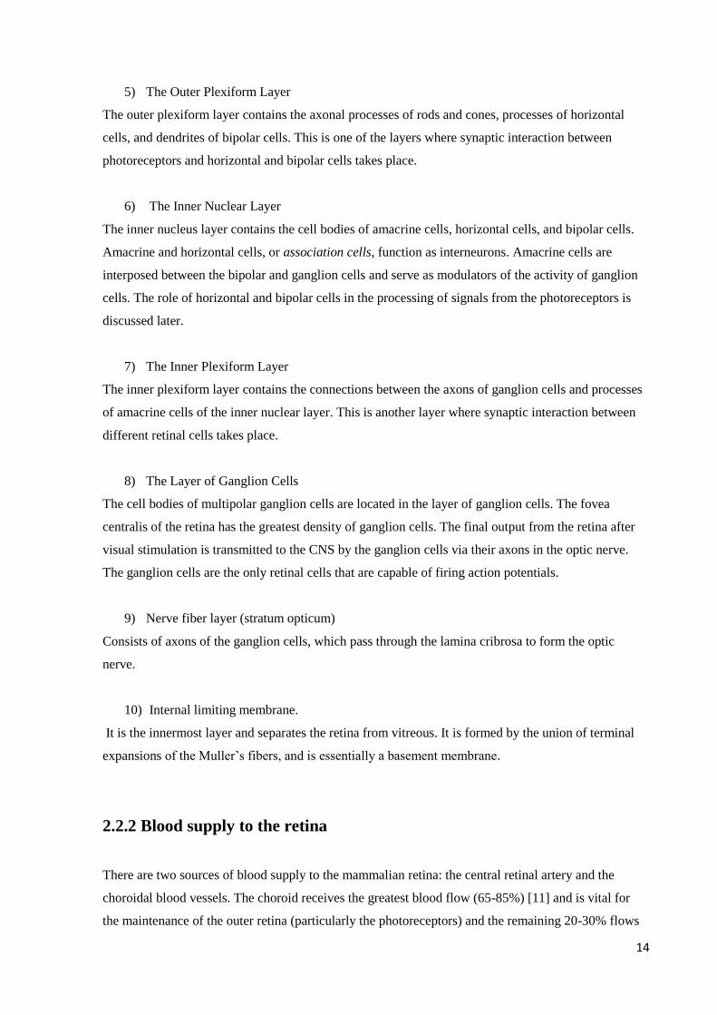
It is an area where the cones are concentrated at the maximum density and arranged with the most
efficient packing geometry which is in a hexagonal mosaic. Starting at the outskirts of the fovea,
however, rods gradually appear, and the absolute density of cone receptors progressively decreases.
In the primate fovea (including humans) the ratio of ganglion cells to photoreceptors is about 2.5;
almost every ganglion cell receives data from a single cone, and each cone feeds onto between 1 and 3
ganglion cells.[13] . Therefore, the acuity of foveal vision is limited only by the density of the cone
mosaic, and the fovea is the area of the eye with the highest sensitivity to fine details [14].
Cones in the central fovea express pigments that are sensitive to green and red light. These cones are
the 'midget' pathways that also underpin high acuity functions of the fovea.
The fovea comprises less than 1% of retinal size but takes up over 50% of the visual cortex in the
brain.[15] In the fovea there are neither cones S nor the rods; without cones S are avoided phenomena
of chromatic aberration in the area of maximum visual acuity.
Fig. 5: The spatial mosaic f the human cones. Cross sections of the human retina at the level of the inner segment showing (A) cones in the
fovea and (B) cones in the periphery.
16
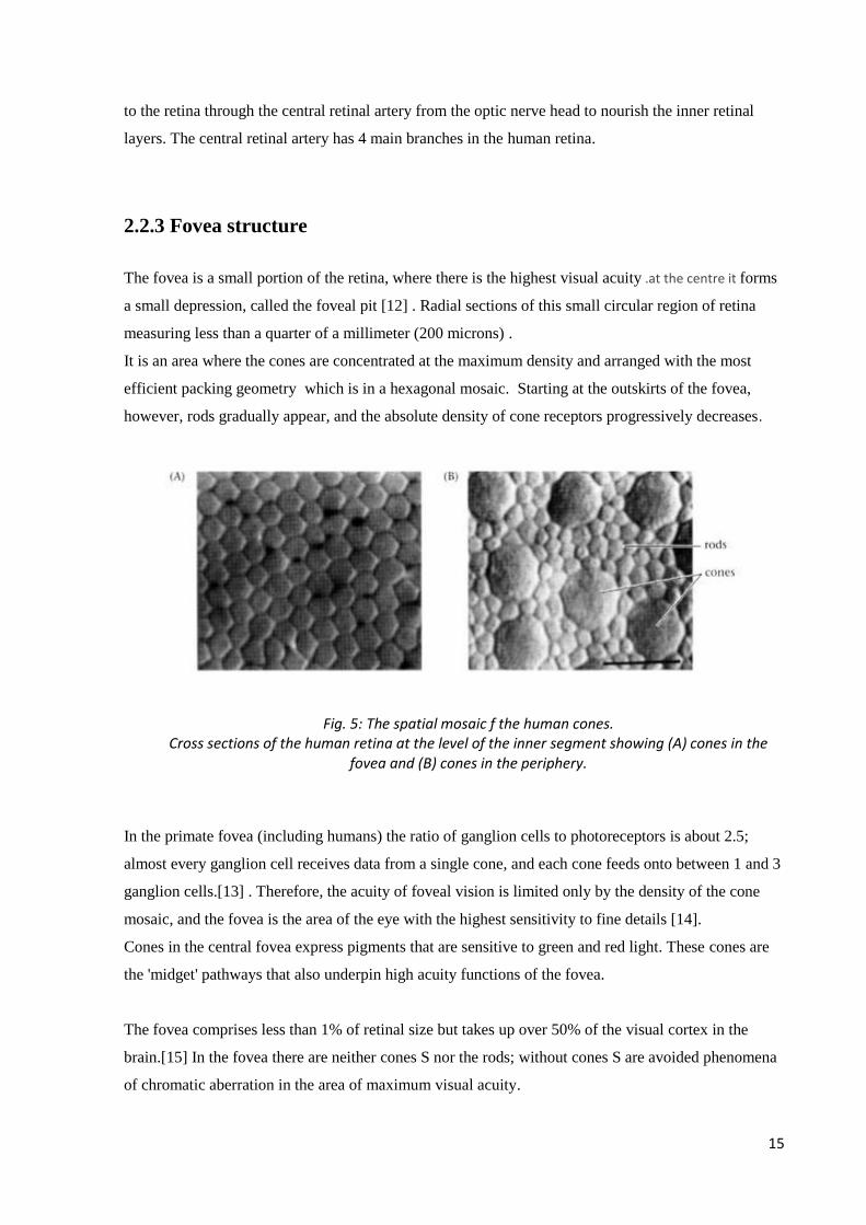
Fig. 7: (A) fundus photo of a normal human macula, optic nerve and blood vessels around the
fovea. B) Optical coherence tomography (OCT) images of the same normal macular in the area that
is boxed in green above (A). The foveal pit (arrow) and the sloping foveal walls with dispelled inner
retina neurons (green and red cells) are clearly seen. Blue cells are the packed photoreceptors,
primarily cones, above the foveal center (pit).
Fig. 6: Vertical section of the human fovea from Yamada (1969). Os,outer segment; is,inner segment; OLM, outer limiting membrane; ONL, outer nuclear layer; H,
henler filbers; INL, inner nuclear layer; ILM, inner limiting membrane; G, ganglion cells.
17
2.2.4 Macula lutea
The whole foveal area including foveal pit, foveal slope, parafovea and perifovea is considered the
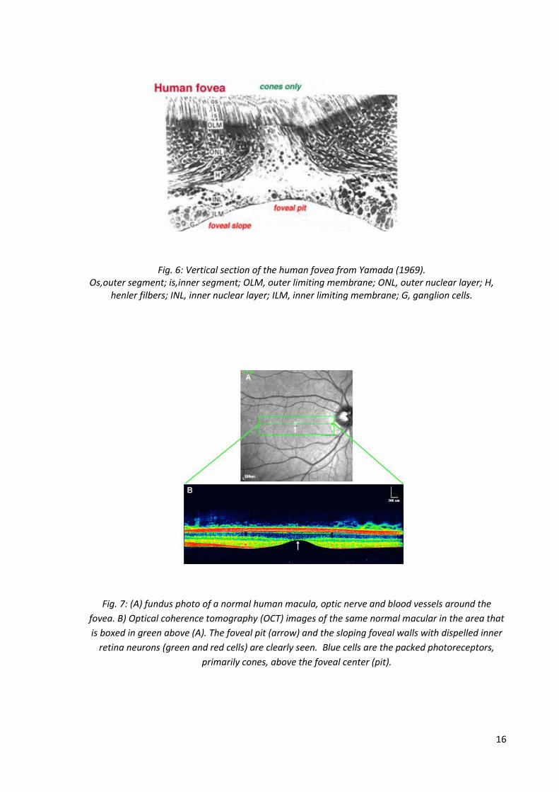
macula of the human eye. Familiar to ophthalmologists is a yellow pigmentation to the macular area
known as the macula lutea (Fig. 7).
This pigmentation is the reflection from yellow screening pigments, the xanthophyll carotenoids
zeaxanthin and lutein[16] present in the cone axons of the Henle fibre layer. The macula lutea is
thought to act as a short wavelength filter, additional to that provided by the lens (Rodieck, 1973). As
the fovea is the most essential part of the retina for human vision, protective mechanisms for avoiding
bright light and especially ultraviolet irradiation damage are essential. For, if the delicate cones of our
fovea are destroyed we become blind.
2.2.5 Ganglion cell fiber layer
The ganglion cell axons run in the nerve fiber layer above the inner limiting membrane towards the
optic nerve head in a arcuate form (Fig. 8, streaming pink fibers). The fovea is, of course, free of a
nerve fiber layer as the inner retina and ganglion cells are pushed away to the foveal slope. The
central ganglion cell fibers run around the foveal slope and sweep in the direction of the optic nerve.
Peripheral ganglion cell axons continue this arcing course to the optic nerve with a dorso/ventral split
along the horizontal meridian (Fig. 8). Retinal topography is maintained in the optic nerve, through
the lateral geniculate to the visual cortex.
Fig. 8: Opthalmoscopic appearance
of the retina to show the macula
lutea (yellow around fovea)
18
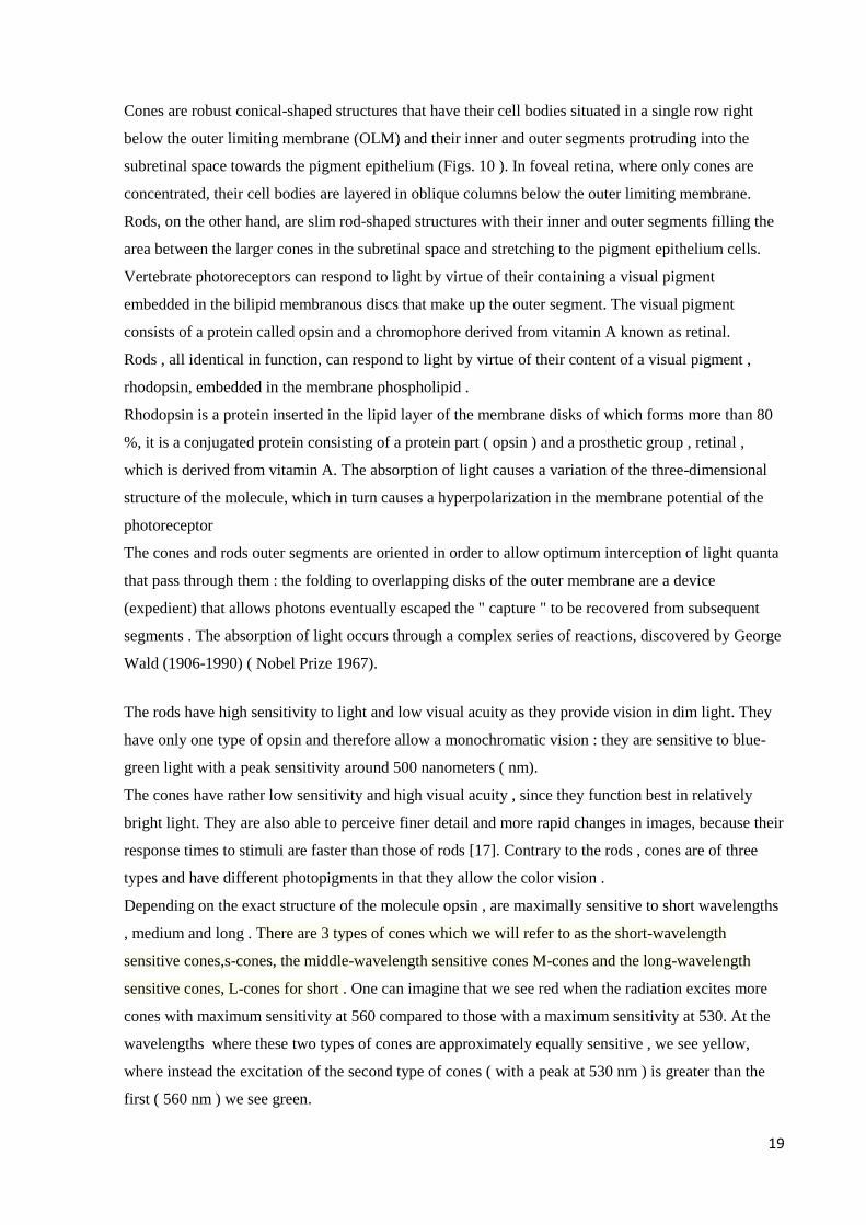
2.2.6 Photoreceptors
Two or three types of cone photoreceptor and a single type of rod photoreceptor are present in the
normal mammalian retina. In vertical sections of retina prepared for light microscopy with the rods
and cones nicely aligned, the rods and cones can be distinguished rather easily.
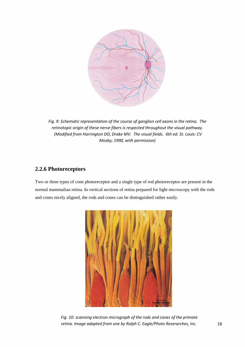
Fig. 9: Schematic representation of the course of ganglion cell axons in the retina. The
retinotopic origin of these nerve fibers is respected throughout the visual pathway.
(Modified from Harrington DO, Drake MV. The visual fields. 6th ed. St. Louis: CV
Mosby; 1990, with permission)
Fig. 10: scanning electron micrograph of the rods and cones of the primate
retina. Image adapted from one by Ralph C. Eagle/Photo Reserarches, Inc.
19
Cones are robust conical-shaped structures that have their cell bodies situated in a single row right
below the outer limiting membrane (OLM) and their inner and outer segments protruding into the
subretinal space towards the pigment epithelium (Figs. 10 ). In foveal retina, where only cones are
concentrated, their cell bodies are layered in oblique columns below the outer limiting membrane.
Rods, on the other hand, are slim rod-shaped structures with their inner and outer segments filling the
area between the larger cones in the subretinal space and stretching to the pigment epithelium cells.
Vertebrate photoreceptors can respond to light by virtue of their containing a visual pigment
embedded in the bilipid membranous discs that make up the outer segment. The visual pigment
consists of a protein called opsin and a chromophore derived from vitamin A known as retinal.
Rods , all identical in function, can respond to light by virtue of their content of a visual pigment ,
rhodopsin, embedded in the membrane phospholipid .
Rhodopsin is a protein inserted in the lipid layer of the membrane disks of which forms more than 80
%, it is a conjugated protein consisting of a protein part ( opsin ) and a prosthetic group , retinal ,
which is derived from vitamin A. The absorption of light causes a variation of the three-dimensional
structure of the molecule, which in turn causes a hyperpolarization in the membrane potential of the
photoreceptor
The cones and rods outer segments are oriented in order to allow optimum interception of light quanta
that pass through them : the folding to overlapping disks of the outer membrane are a device
(expedient) that allows photons eventually escaped the " capture " to be recovered from subsequent
segments . The absorption of light occurs through a complex series of reactions, discovered by George
Wald (1906-1990) ( Nobel Prize 1967).
The rods have high sensitivity to light and low visual acuity as they provide vision in dim light. They
have only one type of opsin and therefore allow a monochromatic vision : they are sensitive to blue-
green light with a peak sensitivity around 500 nanometers ( nm).
The cones have rather low sensitivity and high visual acuity , since they function best in relatively
bright light. They are also able to perceive finer detail and more rapid changes in images, because their
response times to stimuli are faster than those of rods [17]. Contrary to the rods , cones are of three
types and have different photopigments in that they allow the color vision .
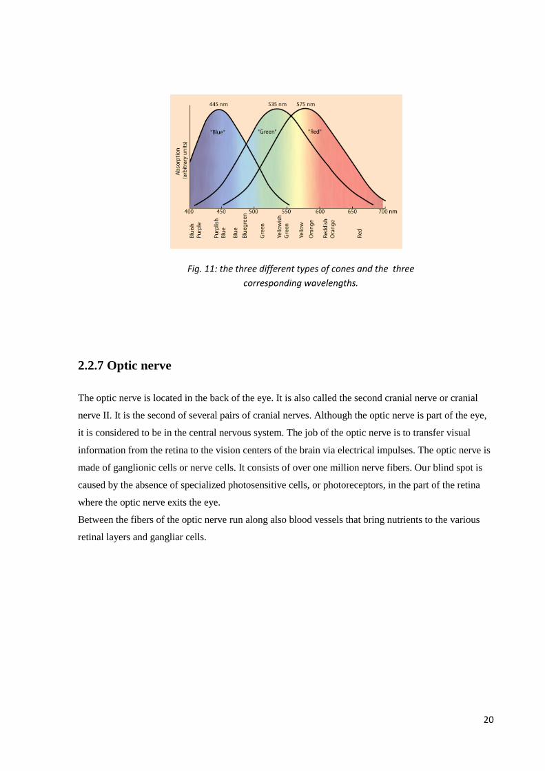
Depending on the exact structure of the molecule opsin , are maximally sensitive to short wavelengths
, medium and long . There are 3 types of cones which we will refer to as the short-wavelength
sensitive cones,s-cones, the middle-wavelength sensitive cones M-cones and the long-wavelength
sensitive cones, L-cones for short . One can imagine that we see red when the radiation excites more
cones with maximum sensitivity at 560 compared to those with a maximum sensitivity at 530. At the
wavelengths where these two types of cones are approximately equally sensitive , we see yellow,
where instead the excitation of the second type of cones ( with a peak at 530 nm ) is greater than the
first ( 560 nm ) we see green.
20
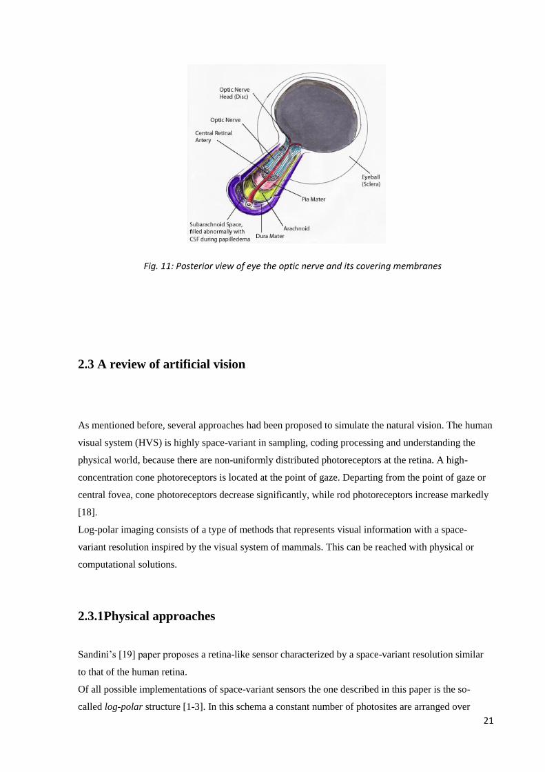
2.2.7 Optic nerve
The optic nerve is located in the back of the eye. It is also called the second cranial nerve or cranial
nerve II. It is the second of several pairs of cranial nerves. Although the optic nerve is part of the eye,
it is considered to be in the central nervous system. The job of the optic nerve is to transfer visual
information from the retina to the vision centers of the brain via electrical impulses. The optic nerve is
made of ganglionic cells or nerve cells. It consists of over one million nerve fibers. Our blind spot is
caused by the absence of specialized photosensitive cells, or photoreceptors, in the part of the retina
where the optic nerve exits the eye.
Between the fibers of the optic nerve run along also blood vessels that bring nutrients to the various
retinal layers and gangliar cells.
Fig. 11: the three different types of cones and the three
corresponding wavelengths.
21
2.3 A review of artificial vision
As mentioned before, several approaches had been proposed to simulate the natural vision. The human
visual system (HVS) is highly space-variant in sampling, coding processing and understanding the
physical world, because there are non-uniformly distributed photoreceptors at the retina. A high-
concentration cone photoreceptors is located at the point of gaze. Departing from the point of gaze or
central fovea, cone photoreceptors decrease significantly, while rod photoreceptors increase markedly
[18].
Log-polar imaging consists of a type of methods that represents visual information with a space-
variant resolution inspired by the visual system of mammals. This can be reached with physical or
computational solutions.
2.3.1Physical approaches
Sandini’s [19] paper proposes a retina-like sensor characterized by a space-variant resolution similar
to that of the human retina.
Of all possible implementations of space-variant sensors the one described in this paper is the so-
called log-polar structure [1-3]. In this schema a constant number of photosites are arranged over
Fig. 11: Posterior view of eye the optic nerve and its covering membranes

22
concentric rings (the polar part of the representation) giving rise to a linear increase of the receptor's
spacing with respect to the distance from the central point of the structure (the radius of the concentric
rings). A possible implementation of this arrangement is shown in Figure 12.
Because of the polar structure of the photosensitive array and the increasing size of pixels in the
periphery, retina-like sensor, do not provide images with a standard topology. In fact in the log-polar
format a point in the image plane at polar coordinates (x ,y ) is mapped into a Cartesian plane (log(x),y
). It is worth noting that the mapping is obtained at no computational cost, as it is a direct consequence
of the photosites array and the read-out sequence.
The topology of a log-polar image is shown in Figure 2. Note that radial structures (the petals of the
flower)
correspond to horizontal structures in the log-polar image. In spite of this seemingly distorted image,
the mapping is conformal and, consequently, any local operator used for "standard" images can be
applied without changes[20].
A first solid-state realization of a log-polar sensor was realized at the end of '90 using CCD technology
[21].
Such technology had some disadvantages that have been solved through CMOS (the size of the
smallest possible pixel was about 30 μm , the sensor had a blind “wedge” because of a read-out shift
register, the increase of pixel's size with eccentricity posed some problems because of the relationship
between the sensitivity of pixels and their size [22]).
Figure 12: Layout of receptor's placing for a log-polar structure composed of 12 rings with 32 pixels each. The pixels marked in black follow a logarithmic spiral.
Figure 13: Left: space variant image obtained by remapping an image acquired by a log-polar sensor. Note the increase in pixels size with eccentricity. Right: Logpolar image acquired by a retina-like sensor. Horizontal lines in the log-polar image are mapped into rings to obtain the re-mapped image shown on the right
23
For example, this pixel has a logarithmic response to illumination and, consequently, the sensitivity of
the largest and smaller pixels is comparable.
More their most recent CMOS implementation was realized using a 0.35 μ m technology that allowed
to have a fourfold increase in number of pixels without increasing the size of the sensor and have a
better coverage of the central part (foveal) removing some of the drawbacks of the previous
implementation.
Thanks to such a techonology it has been possible to reach a high value of the parameter Q (ratio
between sensor's size and size of the smallest pixel) without reducing the figure R (the ratio between
the largest and the smallest pixels ) measuring the "space-variancy" of the sensor.
Except that improvements, such a device has the main limit in the central area, exactly where
resolution should be maximum, is not completely covered by sensors.
2.3.2 Computable methods
Zoujing [23] presents a new computable method to simulate distribution of retina photoreceptors for
space variant resolution imaging. When a human observer gazes at a point in a real word image, a
variable resolution image, as a biological result, is transmitted through the front visual channel into the
high level processing units in the human brain. By taking advantage of this fact, this no-uniform
resolution processing can be applied to digital imaging or video transmission. This application would
be valuable if the network connection between the user and the image server is slow. In this case
image compression algorithms can be vital. However, in the process of simulated HVS (human vision
system) perception, high-fidelity vision would be maintained around the point of gaze, while departing
from it, varied resolution information is transmitted according to the fact of HVS perception. From
the information processing point of view, image processing simulation biological retinal model is
more efficient than traditional methods. The motivation behind foveation image procession is that
there exists considerable high-frequency information redundancy in the peripheral regions, thus a
much more efficient representation of images can be obtained by removing or reducing such
redundancy for implementing low bandwidth method using Gaussian multi-resolution pyramids
(filters).
24
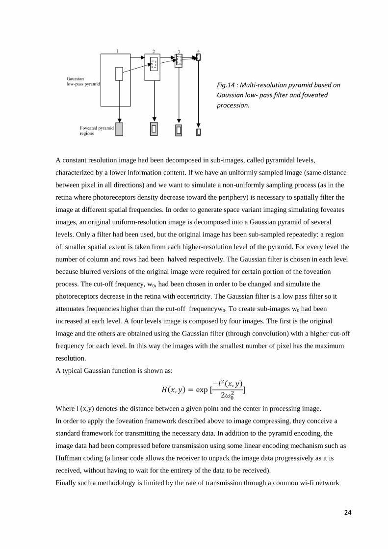
A constant resolution image had been decomposed in sub-images, called pyramidal levels,
characterized by a lower information content. If we have an uniformly sampled image (same distance
between pixel in all directions) and we want to simulate a non-uniformly sampling process (as in the
retina where photoreceptors density decrease toward the periphery) is necessary to spatially filter the
image at different spatial frequencies. In order to generate space variant imaging simulating foveates
images, an original uniform-resolution image is decomposed into a Gaussian pyramid of several
levels. Only a filter had been used, but the original image has been sub-sampled repeatedly: a region
of smaller spatial extent is taken from each higher-resolution level of the pyramid. For every level the
number of column and rows had been halved respectively. The Gaussian filter is chosen in each level
because blurred versions of the original image were required for certain portion of the foveation
process. The cut-off frequency, w0, had been chosen in order to be changed and simulate the
photoreceptors decrease in the retina with eccentricity. The Gaussian filter is a low pass filter so it
attenuates frequencies higher than the cut-off frequencyw0. To create sub-images w0 had been
increased at each level. A four levels image is composed by four images. The first is the original
image and the others are obtained using the Gaussian filter (through convolution) with a higher cut-off
frequency for each level. In this way the images with the smallest number of pixel has the maximum
resolution.
A typical Gaussian function is shown as:
Where l (x,y) denotes the distance between a given point and the center in processing image.
In order to apply the foveation framework described above to image compressing, they conceive a
standard framework for transmitting the necessary data. In addition to the pyramid encoding, the
image data had been compressed before transmission using some linear encoding mechanism such as
Huffman coding (a linear code allows the receiver to unpack the image data progressively as it is
received, without having to wait for the entirety of the data to be received).
Finally such a methodology is limited by the rate of transmission through a common wi-fi network
Fig.14 : Multi-resolution pyramid based on
Gaussian low- pass filter and foveated
procession.
25
and has a not negligible computational complexity in terms of development of the entire pyramidal
structure and in data transmission.
In his paper Traver surveys the application of log-polar imaging in robotic vision, particularly in visual
attention, target tracking, egomotion estimation, and 3D perception.
Both natural and artificial visual systems have to deal with large amounts of information coming from
the surrounding environment. To address this problem the visual system of many animals exhibits a
non-uniform structure, where the receptive fields1 represent certain parts of the visual field more
densely and acutely. In the case of mammals retinas present a unique high resolution area in the center
of the visual field, called the fovea. The distribution of receptive fields within the retina is fixed and
the fovea can be redirected to other targets by ocular movements. The same structure is also
commonly used in robot systems with moving cameras [25] [26]. Log-polar mapping is a geometrical
image transformation that attempts to emulate the topological reorganization of visual information
from the retina to the visual cortex of primates. There are different ways to obtain log-polar images
using software and/ or hardware-based solutions
They believe that using sensors with sensitive elements arranged following a log-polar pattern has a
great drawback . It is represented by the technical obstacles faced either during their design and
construction or even during their usage, which limits the range of applications. Furthermore, the
hardcoded geometry layout makes it very difficult, if not impossible, to experimenting with different
sensor parameters.
At the same time, even if a software approach has a remarkable flexibility in setting the log-polar
parameters they have the unavoidable cost of obtaining the log-polar image from the Cartesian image.
This may be a drawback in real applications. To overcome this problem and still count on the
flexibility of software, they believe that the best solution is an intermediate one. It is represented by
virtual log-polar sensors [27] [28]. This alternative still needs Cartesian images as input, but the
implementation of the log-polar mapping is performed in special-purpose hardware cards, thus making
the conversion faster while providing the possibility of setting the sensor parameters.
Finally, Cormak proposes a paper where he focuses on the processing done by the early levels of the
human vision system to highlight the importance of computational models of the human perception of
the world.
He shows that the main functions performed by the major structures of human vision are filters.
Lowpass filtering by the optics and sampling by the receptor mosaic, the retina and the thalamus cells
filtering. The photoreceptors themselves filter along the dimension of time and wavelength and the
LGN cells (lateral geniculate nucleus of the thalamus) in 2D Fourier plane are circularly symmetric
bandpass filter. Gangliar cells are spatio-temporal bandpass filter. Finally cells in the primary visual
26
cortex can be thought of as banks of spatiotemporal filters that tile the visual world in several
dimensions and, in so doing, determine the envelope of information to which we have access.
For each level, mathematical models that have been developed. That being so, the author reaffirms the
importance of a computational approach because it’s the best way to describe the main biological
structure and their functions of the human vision system.
References
[1] “The Eye: The Physiology of Human Perception, edited by Kara Rogers Britannic, Educational
Publishing].
[2] “Clinical anatomy of the eye”, Richard S. Snell, Michael A. Lemp, pubblicato da Blackwell
Science, 1998].
[3] [4] [5] [7] Encyclopaedia Britannica.
[6] “Dictionary of Eye Terminology”. Cassin, B. and Solomon, S. Gainsville, Florida: Triad
Publishing Company, 1990.
[8] “Anatomy and physiology of the human eyeball in the normal state”, dr. Maximilian Salzmann,
stampato da The University of Chicago Press, 1912.
[9] http://retina.anatomy.upenn.edu/~lance/eye/eye.htm.
[10] “Dynamic fields and waves”, Andrew Norton, The Physical World course, Institute Of Physics
Publishing, 2000, p.137
[11] Henkind et al., 1979.
[12] Polyak, 1941.
[13] “Cell density ratios in a foveal patch in macaque retina”. Ahmad et al., 2003.. Vis.
Neurosci. 20:189-209).
[14 ] “Light:Student Guide and Source Book” Smithsonian/The National Academies, . Carolina
Biological Supply Company, 2002. ISBN 0-89278-892-5.
[15] “Experiencing Sensation and Perception”, Krantz, John H. (1 October 2012). Pearson
Education. ISBN 978-0-13-097793-9.OCLC 711948862. Retrieved 6 April 2012. Available online
ahead of publication.
[16] Balashov and Bernstein, 1998.
[17] “Principles of Neural Science” (4th ed.). Kandel, E.R.; Schwartz, J.H, and Jessell, T. M. (2000).
New York: McGraw-Hill. pp. 507–513.
27
[18] Wandell, 1995; Cormack,2000.
[19 ] “A retina-like CMOS sensor and its applications”. Sandini, Giulio, et al. “Sensor Array and
Multichannel Signal Processing Workshop”. 2000. Proceedings of the 2000 IEEE. IEEE, 2000.
[20 ] “Logarithmic Spiral Grids for Image Processing and Display”. Weiman, C.F.R. and G. Chaikin,
Comp. Graphic and Image Process.,, 1979. 11: p. 197—226.
[21] [22] “A Foveated Retina-like Sensor Using CCD Technology” Spiegel, J.V.d., et al.,. 1989, De
Kluwer.
[23] “Simulated distribution of the retinal photoreceptors for space variant resolution
imaging”.Zoujin Li, W. Shi and Zhi Zhong,
[24 ] “A review of log polar imaging for visual perception in robotics”.V. Javeier Traver, Alexandre
Bernardino,
[25] “Binocular tracking: Integrating perception and control”, A. Bernardino, J. Santos-Victor,
IEEE Transactions on Robotics and Automation 15 (6) (1999) 1080_1094.
[26] “A miniature space-variant active vision system”, B. Bederson , Ph.D. Thesis, New York
University, 1992.
[27] “A programmable video image remapper, in: SPIE Conf. on Pattern Recognition and Signal
Processing, in: Digital and Optical Shape Representation and Pattern Recognition”, vol. 938, 1988,
pp. 122_128 ”. T.E. Fisher, R.D. Juday,
[28] “VIPOL: A virtual polar-logarithmic sensor, in: Scandinavian Conf. on Image Analysis”, J.R.
del Solar, C. Nowack, B. Schneider, SCIA, Finland, 1997, pp. 739_744”.
28
Chapter 3
LIGHT SCATTERING
As mentioned in the introduction, the filter we realized is based on the light scattering phenomenon by
small spherical particles .
Place a filter which exploits the diffusion phenomenon in front of a vision system, such as a camera ,
allows us to obtain images perceived as " blurred.". This immediately call to mind the concept of
foveal vision , where only the object gazed looks exactly in focus, whereas the whole environment that
comes out of his little round arrives to the brain as a blurry image. Such a device seems to be the best
solution to achieve our goal and that is to create a device to simulate human vision.
Therefore is essential to explain and classify the scattering in order to understand completely how the
filter operate and then characterize it.
In addition to scattering is also necessary to introduce other basic concepts the phenomenon of
scattering is intrinsically linked to . We will explain what is light by three theories, how it spreads and
what polarization means. We will speak about the interaction of light with matter and in specific case
of scattering , we focus on the parameters that characterize the small particles that give rise to this
phenomenon.
3.1 Introduction to light
Light is part of the electromagnetic spectrum, the spectrum is the collection of all waves, which
include visible light, Microwaves, radio waves (AM, FM,SW), X-Rays and Gamma Rays.
In the late 1600s important question were raised, asking if light is made up of particles or is it waves?
Isaac Newton held the theory that light was made up of tiny particles. In 1678, Christian Huygens
believed that light was made up of waves vibrating up and down perpendicular to the direction of the
light travels and therefore formulated a way of visualizing wave propagation. This became know as
“Huygens Principle”. Huygens theory was the successful theory of light wave motion in three
dimensions.
Newton’s theory came first, but the theory of Huygens, better described early experiments.
29
At the time, some experiments conducted in light theory, both the wave theory and particle theory, had
some unexplained phenomenon, Newton could not explain the phenomenon of light interference, this
forced Newton’s particle theory in favour of the wave theory. This difficulty was due to the
unexplained phenomenon of light polarization- scientists were familiar with the fact that wave motion
was parallel to the direction of wave, not perpendicular to the direction of wave travel, as light does.
In 1803, Thomas Young studied the interference of light waves by shining light through a screed with
two slits equally separated, the light emerging from the two slits, spread out according to Huygens’s.
In 1900 Max Plank proposed the existence of a light quantum, a finite packet of energy which depends
on the frequency and velocity of the radiation.
In 1905 Albert Einstein had proposed a solution to the problem of observations made in the behavior
of light having characteristic both wave and particle theory. From work of Plank in emission of light
from hot bodies, Einstein suggested that light is composed of tiny particles called photons and each
photon has energy.
Light theory branches in to the physics of quantum mechanics, which was conceptualized in the
twentieth century. Quantum mechanics deals with behavior of nature on the atomic scale or smaller.
As a result of quantum mechanics, this gave the proof if the dual nature of light and therefore not a
contradiction.
In general a wave is a disturbance or variation that transfers energy progressively from point to point
in a medium and that may take the form of an elastic deformation or of a variation of pressure, electric
or magnetic intensity, electric potential, or temperature. Waves are important because all the
information that we receive, auditory and visual, are transmitted through them. The light and sound
have in fact typical properties of the waves and in a simple treatise can be considered as waves. [1]
In general there are two types of waves: transverse waves in which the displacement, i.e. the
movement caused by the disturbance, is perpendicular to the direction in which the perturbation moves
and longitudinal waves where the displacement is parallel to the direction of propagation.
Mathematically, the simplest waves are "periodic waves" that continue undisturbed for long distances
ideally for infinite times.
The sine wave is the fundamental waveform in nature. When dealing with light waves, we refer to the
sine wave. To describe sin we need only to know its frequency and the speed of the disturbance, called
phase velocity, in the medium.
The frequency is the number of peaks that will travel past a point in one second and is set by the
source.
As consequence of the conservation of energy, the frequency does not change as the wave travels from
one medium to another. Since the frequency remains unchanged, the wavelength of a wave is different
from a medium to another. Moreover, the speed of propagation through a medium is lower than in the
vacuum.
The relationship of wavelength, speed of disturbance and frequency is given by the equation:
30
λ= f
v
This equation tells us that for a given speed of propagation, the higher the frequency and the smaller
the wavelength.
There are different types of waves, for example, a wave on water of a lake, waves of a vibrating string,
sound waves in the air that allow us to feel, radio waves, TV waves or X-rays. The last three examples
are electromagnetic waves, while the others are mechanical waves. Only a small portion of the
electromagnetic spectrum is visible to the human eye and that is what we usually call light. In this
context, the equation seen previously, becomes:
λ = f
c
This shows an important property of electromagnetic waves: the speed of propagation is the same for
all waves and is equal to the speed of light in vacuum.[2]
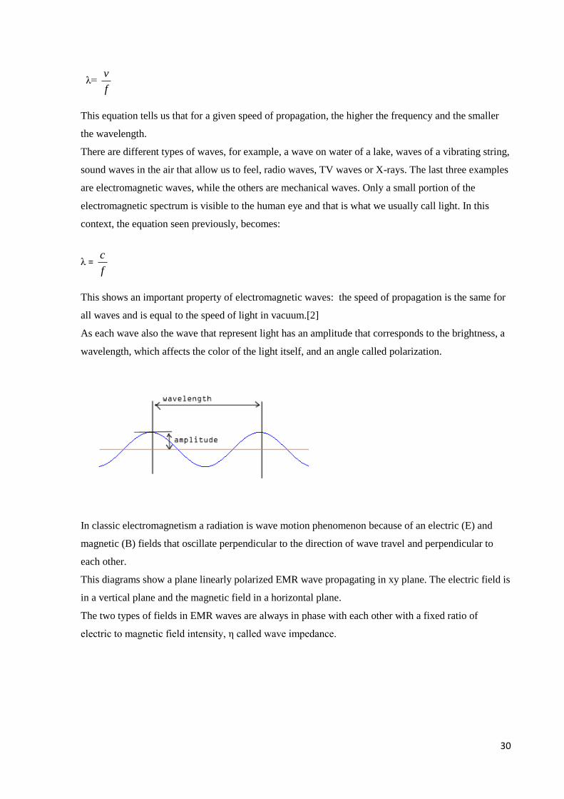
As each wave also the wave that represent light has an amplitude that corresponds to the brightness, a
wavelength, which affects the color of the light itself, and an angle called polarization.
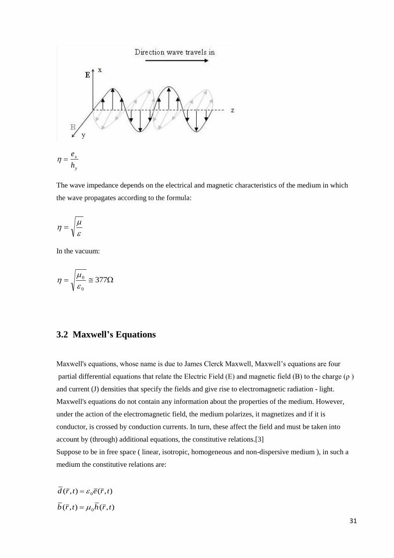
In classic electromagnetism a radiation is wave motion phenomenon because of an electric (E) and
magnetic (B) fields that oscillate perpendicular to the direction of wave travel and perpendicular to
each other.
This diagrams show a plane linearly polarized EMR wave propagating in xy plane. The electric field is
in a vertical plane and the magnetic field in a horizontal plane.
The two types of fields in EMR waves are always in phase with each other with a fixed ratio of
electric to magnetic field intensity, η called wave impedance.
31
y
x
h
e
The wave impedance depends on the electrical and magnetic characteristics of the medium in which
the wave propagates according to the formula:
In the vacuum:
3770
0
3.2 Maxwell’s Equations
Maxwell's equations, whose name is due to James Clerck Maxwell, Maxwell’s equations are four
partial differential equations that relate the Electric Field (E) and magnetic field (B) to the charge (ρ )
and current (J) densities that specify the fields and give rise to electromagnetic radiation - light.
Maxwell's equations do not contain any information about the properties of the medium. However,
under the action of the electromagnetic field, the medium polarizes, it magnetizes and if it is
conductor, is crossed by conduction currents. In turn, these affect the field and must be taken into
account by (through) additional equations, the constitutive relations.[3]
Suppose to be in free space ( linear, isotropic, homogeneous and non-dispersive medium ), in such a
medium the constitutive relations are:
),(),( 0 tretrd
),(),( 0 trhtrb
32
In which d and b are auxiliary fields; e electric field, h magnetic field. ε0 and μ0 are two universal
constants, called the permittivity of free space and permeability of free space, respectively.
In vacuum ε0 1/(36π)∙10-9
[F/m], and μ0=4π∙10-7
[H/m].
Maxwell’s equations in time domain are:
),(),( trbt
tre
),(),(),( trjtrdt
trh
),(),( trtrd
0),( trb
In which j is the electric current density the electric current per unit area of cross section ΔS , where
S tends to zero. ρ the electric charge per unit volume, where ΔV tends to zero.
The electric density j can be divided in two parts:
),(),(),( 01 trjtrjtrj
In which 1j is produced by electromagnetic field and 0j by generators.
We can see that Maxwell's equations relate the vectors field with the sources of the field itself. They
are a set of four equations ( two vector and two scalar ) corresponding to eight scalar equations . Is
immediately evident that the number of unknowns is greater than the number of equations . If density
of free charge and current density supported by the generators are assigned, the unknowns variables
are represented by the component of the vectors . We should note also that Maxwell's equations are
not all linearly independent . The system of Maxwell is therefore indeterminate ; it can be determined
if we consider others relations about the medium the fields arise. These are the constitutive relations
previously defined. Now suppose to be in absence of sources , and considering the constitutive
relations , the system of Maxwell's equations become :
),(),( 0 trht
tre
),(),( 0 tret
trh
0)),(( 0 tre
),()),(( 0 trtrh
33
Assuming that the fields e and h , usually functions of x, y, z and t, depend only on the z-axis and on
the time t, performing calculation, we obtain D'Alembert’s equation:
2
22
2
2
z
ec
t
e xx
With
00
1
c
And the solution is:
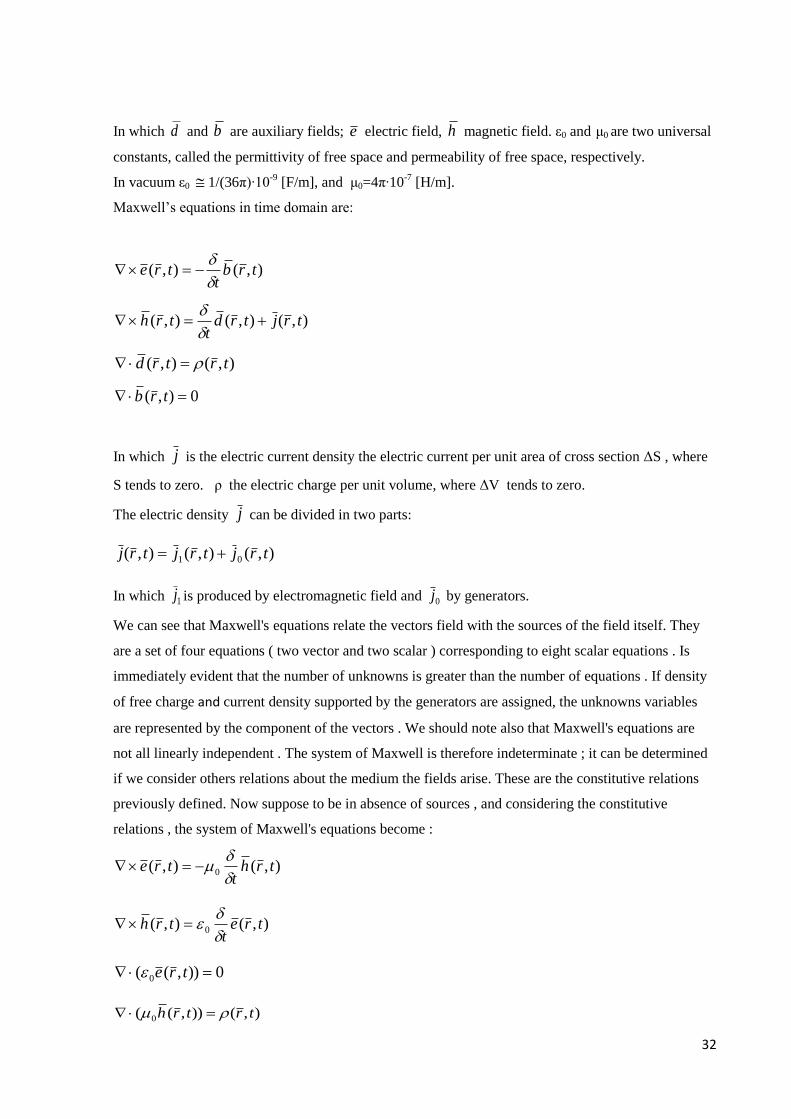
)()( 21 ctzfctzfex
Where f1 and f2 are functions that depend on the specific problem we are dealing with. Since the
medium in question was supposed to be linear, the principle of superposition can be applied. We can
therefore consider only the first part of the solution:
)(1 ctzfex
3. 3 Particle theory of light
Newton proposed that light consists of little particles, which he referred to as corpuscles, with energy
and momentum. When a light particle is deep within a medium, such as water or glass, it is
surrounded on all sides by equal numbers of these particles. Suppose there is an attractive force
Fig. 1. A wave travelling in the x direction with unchanging shape and with velocity c. at time t=0
the shape is ψ=f(x) and at time t it is ψ=F(x - ct)
34
between the light particles and the matter particles. Then deep within a medium, these forces cancel
each other out and there is no net force on the light particle. Then, according to Newton’s first law, the
light particle will continue moving in a straight line since no net force acts on it.
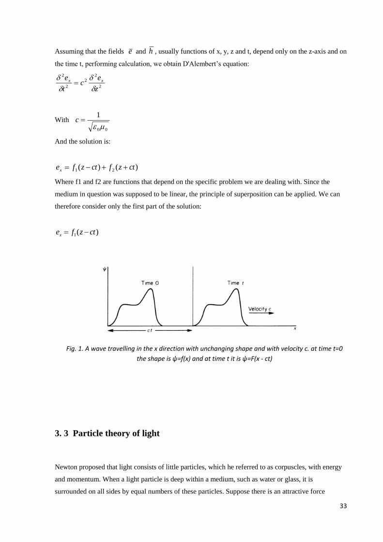
Many known properties of light could be explained easily by a particle model. For example it was
known that when light reflects from a smooth surface, the angle of incidence is equal to the angle of
reflection.
As we shall see, a key property for the particle theory is refraction.
Instead, if the body is porous ( constituted in such a way that between atom and atom there are wide
gaps) the particles pass through it. As they suffer the gravitational attraction , are accelerated. Because
of this, the speed of light is greater in a denser medium and the particles are diverted (in straight
directions) with compared to the original trajectory.
Newton concluded that light is composed of coloured particles which combine to appear white. He
introduced the term 'colour spectrum' and, although the spectrum appears continuous, with no distinct
boundaries between the colours, he chose to divide it into seven
His explanation for the fact that a prism separates a beam of white light into the colors of the rainbow
was simple. We have seen that red light refracts least, and violet light most. Newton stated that the
mass of the
light particle varied with color. Red light particles have more mass than violet, consequently they will
be deflected less upon crossing an interface between materials. He assumed all light particles
experience the same force on crossing an interface. What differs among them is their inertia. Red light
particles with more inertia will be deflected less by the same force than violet light particles.
Fig.2 : Reflection and refraction
35
3.4 Quantum theory
According to modern quantum physics created by Einstein, the particles that make up atoms are made
from tiny concentrated energy, of those many have a dual nature : wave and particle . Precisely the
matter at the subatomic level has the typical characteristics of the waves and only when we observe
this the matter has a corpuscular behavior .
In the quantum theory of light, light exists as tiny packets called photons. So the brightness of the light
corresponds to the number of photons , the color to the energy contained in each photon and four
letters (x, y, z, t ) indicate the polarization .
We might ask which interpretation is correct. Both , actually.
It seems that the electromagnetic radiation can have both wave and particle properties.
For the purposes of this paper , we will discuss only the light from the point of view of the wave , also
remembering that they're both valid.
The light is defined as the electromagnetic radiation that has a wavelength ranging from 330
nm(violet) to about 770 nm (red) and may be perceived by the normal unaided human eye. Thus light
takes up a very small portion of the spectrum . The visible spectrum ranges from the long radio waves,
which are often thought of as the propagation and the oscillating electric fields , short X-rays and
gamma rays, which are imagined as energetic particles . It’s important to remember that there is no
fundamental difference between one and another portion of the electromagnetic spectrum . A radio
wave is a broad- wavelength and x-rays on the other hand have short wavelength , but both are
electromagnetic radiation and their behavior is governed by the same rules.
But if all these waves are basically the same thing , we might ask why we do not see radio waves as
we see the light? Or, why do we need special infrared lamps to warm things up ? Although the various
portions of the electromagnetic spectrum are governed by the same laws, their wavelengths and their
different energies implies that they have different effects on matter. Radio waves for example have a
length so wide and an energy that our eyes are not able to receive and they pass through our bodies .
An antenna wire with a special electronics to capture and amplify radio waves is necessary.
Similarly, the infrared radiation is easily absorbed by the material and converted into heat, X-rays
instead have a wavelength which passes through soft tissue but is stopped by the bone. The
exceptional variety of the electromagnetic spectrum is the result of the same law applied to different
wavelengths and energies. The quantum nature of a wave, which is responsible of the obvious
differences between the gamma ray and a radio waves, occurs only when the waves interact with
matter. It has been shown that the waves exchange energy and momentum with their generators and
absorbers only in discrete packets, in accordance with the quantum laws. These packets of energy,
called quanta, are the photons.
36
3.5 Wave propagation
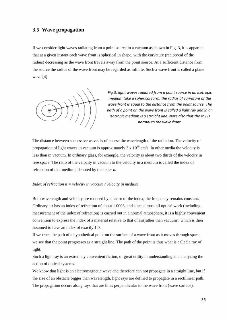
If we consider light waves radiating from a point source in a vacuum as shown in Fig. 3, it is apparent
that at a given instant each wave front is spherical in shape, with the curvature (reciprocal of the
radius) decreasing as the wave front travels away from the point source. At a sufficient distance from
the source the radius of the wave front may be regarded as infinite. Such a wave front is called a plane
wave [4]
The distance between successive waves is of course the wavelength of the radiation. The velocity of
propagation of light waves in vacuum is approximately 3 x 10¹⁰
cm/s. In other media the velocity is
less than in vacuum. In ordinary glass, for example, the velocity is about two thirds of the velocity in
free space. The ratio of the velocity in vacuum to the velocity in a medium is called the index of
refraction of that medium, denoted by the letter n.
Index of refraction n = velocitv in vaccum / velocity in medium
Both wavelength and velocity are reduced by a factor of the index; the frequency remains constant.
Ordinary air has an index of refraction of about 1.0003, and since almost all optical work (including
measurement of the index of refraction) is carried out in a normal atmosphere, it is a highly convenient
convention to express the index of a material relative to that of air(rather than vacuum), which is then
assumed to have an index of exactly 1.0.
If we trace the path of a hypothetical point on the surface of a wave front as it moves through space,
we see that the point progresses as a straight line. The path of the point is thus what is called a ray of
light.
Such a light ray is an extremely convenient fiction, of great utility in understanding and analyzing the
action of optical systems.
We know that light is an electromagnetic wave and therefore can not propagate in a straight line, but if
the size of an obstacle bigger than wavelength, light rays are defined to propagate in a rectilinear path.
The propagation occurs along rays that are lines perpendicular to the wave front (wave surface).
Fig.3: light waves radiated from a point source in an isotropic
medium take a spherical form; the radius of curvature of the
wave front is equal to the distance from the point source. The
path of a point on the wave front is called a light ray and in an
isotropic medium is a straight line. Note also that the ray is
normal to the wave front.
37
Geometric optics studies therefore the "behavior" of rays, as if light was formed by particles moving
along these rays.
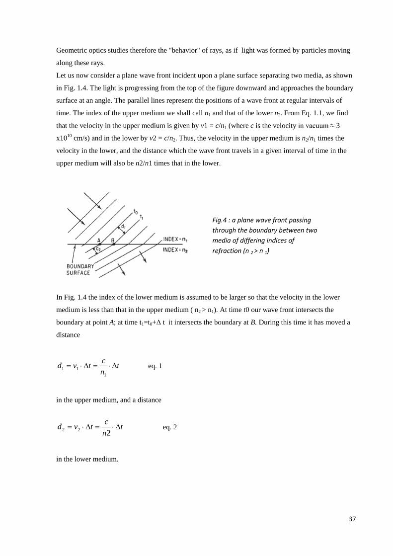
Let us now consider a plane wave front incident upon a plane surface separating two media, as shown
in Fig. 1.4. The light is progressing from the top of the figure downward and approaches the boundary
surface at an angle. The parallel lines represent the positions of a wave front at regular intervals of
time. The index of the upper medium we shall call n1 and that of the lower n2. From Eq. 1.1, we find
that the velocity in the upper medium is given by v1 = c/n1 (where c is the velocity in vacuum ≈ 3
x1010
cm/s) and in the lower by v2 = c/n2. Thus, the velocity in the upper medium is n2/n1 times the
velocity in the lower, and the distance which the wave front travels in a given interval of time in the
upper medium will also be n2/n1 times that in the lower.
In Fig. 1.4 the index of the lower medium is assumed to be larger so that the velocity in the lower
medium is less than that in the upper medium ( n2 > n1). At time t0 our wave front intersects the
boundary at point A; at time t1=t0+Δ t it intersects the boundary at B. During this time it has moved a
distance
tn
ctvd
1
11 eq. 1
in the upper medium, and a distance
tn
ctvd
222 eq. 2
in the lower medium.
Fig.4 : a plane wave front passing
through the boundary between two
media of differing indices of
refraction (n 2 > n 1)

38
In Fig. 5 we have added a ray to the wave diagram; this ray is the path of the point on the wave front
which passes through point B on the surface and is normal to the wave front. If the lines represent the
positions of the wave at equal intervals of time, AB and BC, the distances between intersections, must
be equal. The angle between the wave front and the surface (I1 or I2) is equal to the angle between the
ray (which is normal to the wave) and the normal to the surface XX′.
Thus we have from Fig. 5
2
2
1
1
sinsin I
dBC
I
dAB eq. 3a
and if we substitute the values of d1 and d2 from Eq. 3, we get
2211 sinsin In
tc
In
tc
eq. 3b
which, after canceling and rearranging, yields
2211 sinsin InIn eq. 4
This expression is the basic relationship by which the passage of light rays is traced through optical
systems. It is called Snell’s law after one of its discoverers. Since Snell’s law relates the sines of the
angles between a light ray and the normal to the surface, it is readily applicable to surfaces other than
the plane which we used in the example above; the path of a light ray may be calculated through any
surface for which we can determine the point of intersection of the ray and the normal to the surface at
Fig. 5: Refraction of a wave (ray) at the
interface between two media of different
refractive indices.
39
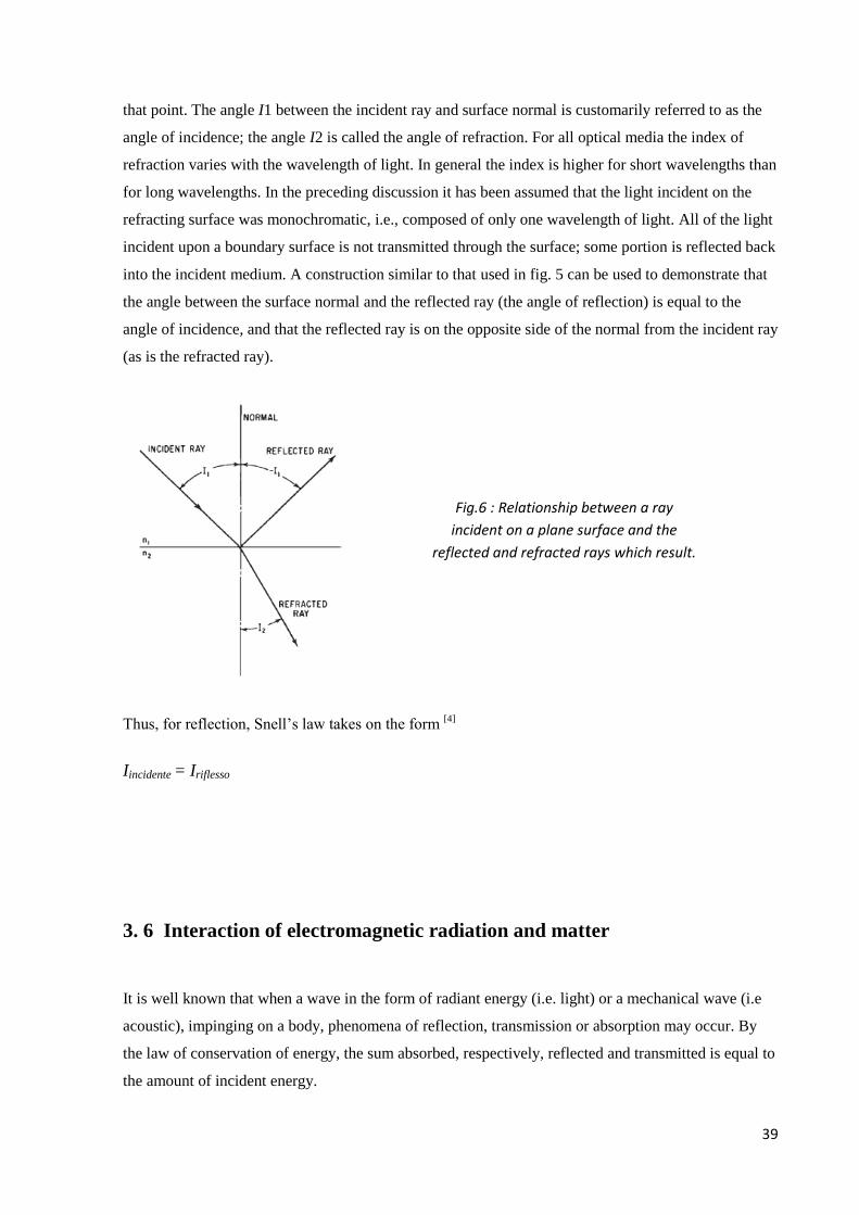
that point. The angle I1 between the incident ray and surface normal is customarily referred to as the
angle of incidence; the angle I2 is called the angle of refraction. For all optical media the index of
refraction varies with the wavelength of light. In general the index is higher for short wavelengths than
for long wavelengths. In the preceding discussion it has been assumed that the light incident on the
refracting surface was monochromatic, i.e., composed of only one wavelength of light. All of the light
incident upon a boundary surface is not transmitted through the surface; some portion is reflected back
into the incident medium. A construction similar to that used in fig. 5 can be used to demonstrate that
the angle between the surface normal and the reflected ray (the angle of reflection) is equal to the
angle of incidence, and that the reflected ray is on the opposite side of the normal from the incident ray
(as is the refracted ray).
Thus, for reflection, Snell’s law takes on the form [4]
Iincidente = Iriflesso
3. 6 Interaction of electromagnetic radiation and matter
It is well known that when a wave in the form of radiant energy (i.e. light) or a mechanical wave (i.e
acoustic), impinging on a body, phenomena of reflection, transmission or absorption may occur. By
the law of conservation of energy, the sum absorbed, respectively, reflected and transmitted is equal to
the amount of incident energy.
Fig.6 : Relationship between a ray
incident on a plane surface and the
reflected and refracted rays which result.
40
Usually we refer to absorption (of light, radio waves, sound, neutrons and the like) to denote the
phenomenon whereby the energy carried by electromagnetic waves ,elastic waves or particles that
propagate in a material medium, gradually decreases along the direction of propagation.
The parameter that determines how far into the material a particular wavelength can penetrate, before
it is absorbed, is the absorption co-efficient. It is defined as ratio between the luminous flux and the
absorbed incident:
incident
absorbed
The transmission is the propagation of an incident ray through a medium without being absorbed or
scattered.
The parameter that determines the spreading ability luminance flux of a medium is transmittance.
Reflectance is the ratio of reflected power to incident power, generally expressed in
decibels or percent.
incident
trasmitted
Finally, reflection occurs when a wave hits the interface between two dissimilar media, so that all of,
or at least part of, the wave front returns into the medium from which it originated. The remaining part
of incident radiant energy that is not reflected, penetrates in the other material as propagating wave
refracted. [5]
The parameter that defines the ability of an object to reflect a luminous flux is know as reflectance and
is defined as follows:
incident
reflected
The reflection can be elastic, if the kinetic energy of the incident particles is kept in the center of mass
[6] and is changed only by the direction of propagation, in the case of the light, if the incident beam is
reflected with the same frequency ; can be inelastic otherwise.
41
3.7 Scattering
Scattering is a general physical process where some forms of radiation are forced to deviate from a
straight trajectory by one or more paths due to localized non-uniformities in the medium through
which they pass.
There are three different type of reflection: specular reflection, diffuse reflection (scattering) and
mixed reflection.
Reflection of light may occur whenever light travels from a medium of a given refractive index into a
medium with a different refractive index. In the most general case, a certain fraction of the light is
reflected from the interface, and the remainder is refracted as it passes into the transparent medium.
When light reflects off a material denser than the external medium, it undergoes a 180° phase
reversal. In contrast, a less dense, lower refractive index material will reflect light in phase. This is an
important principle in the field of thin-film optics.
Specular reflection at a curved surface forms an image which may be magnified or reduced.
The specular reflection occurs if the wavelength of the radiation is much smaller than the surface
discontinuities otherwise it has a diffuse reflection . [7] The specular reflection is observed when a
single incident ray, which forms an angle θi with the normal, produces a single beam reflection angle
θr with respect to the normal. For this is verified θi = θr in accordance with the law of reflection .
Incident ray , normal and emergent ray lie on the same plane.
When light strikes a rough or granular surface, it bounces off in all directions due to the microscopic
irregularities of the interface. This is called diffuse reflection. The exact form of the reflection depends
on the structure of the surface. A common model for diffuse reflection is Lambertian reflectance, in
which the light is reflected in accordance with Lambert's cosine law. Lambert's cosine law says that
the total radiant power observed from a "Lambertian" surface is directly proportional to the cosine of
the angle θ between the observer's line of sight and the surface normal. The law is also known as the
cosine emission law or Lambert's emission law (Johann Heinrich Lambert, Photometria, 1760).
When an area element is radiating as a result of being illuminated by an external source, the
irradiance (energy/time/area) landing on that area element will be proportional to the cosine of the
angle between the illuminating source and the normal. A Lambertian reflector will then reflect this
light according to the same cosine law as a Lambertian emitter.
This means that although the radiance of the surface under diffuse reflection depends on the angle
from the normal to the illuminating source, it will not depend on the angle from the normal to the
observer.
42
In the case of diffuse reflection the incident ray is broken up and re-emitted in multiple directions
irrespective of its original direction , according to what is defined as the scattering profile of the
surface.[8] The deflection is then carried out in a disordered way and largely random .
Generally, however, only elastic interactions ( where there is conservation of energy ) or quite elastic
are treated as elastic scattering processes . Scattering is defined here as energy absorption of incident
light followed by re-emission of part of this light at the same frequency [9].
The origins of light scattering are surface irregularities . From this it follows that volume scattering is
scattering at the surface of particles in a certain volume.
Mixed diffusion is more general and in it the beam undergoes a combination of the previous two
effects : the radiation is reflected , but a main component along the specular direction remains. [10]
Therefore the scattering is a phenomenon in which a wave, light , sound or even a particle, is deviated
in its rectilinear trajectory due to some discontinuities present in the medium of incidence.
Many discontinuities generate scattering , often known as scatterers or scattering centers , as particles ,
bubbles , droplets, density fluctuations in fluids , the crystallites in polycrystalline solids , defects in
monocrystalline solid , rough surfaces , in cell bodies and fibers in tissues. [11]
When radiation is only scattered by one localized scattering center, this is called single scattering, It is
very common that scattering centers are grouped together, and in those cases the radiation may scatter
many times, which is known as multiple scattering. Multiple scattering is here discussed as the
weighted superposition of many single scatterers without interference effects. Multiple scattering with
interference effects is called coherent scattering.
The main difference between the effects of single and multiple scattering is that single scattering can
usually be treated as a random phenomenon and multiple scattering is usually more stochastic.
Because the location of a single scattering center is not usually well known relative to the path of the
radiation, the outcome, which tends to depend strongly on the exact incoming trajectory, appears
random to an observer. This type of scattering would be exemplified by an electron being fired at an
atomic nucleus. In that case, the atom's exact position relative to the path of the electron is unknown
and would be immeasurable, so the exact direction of the electron after the collision is unknown, plus
the quantum-mechanical nature of this particular interaction also makes the interaction random. Single
scattering is therefore often described by probability distributions. With multiple scattering, the
randomness of the interaction tends to be averaged out by the large number of scattering events, so
that the final path of the radiation appears to be a deterministic distribution of intensity. This is
exemplified by a light beam passing through thick fog. Optical elements designed to produce multiple
scattering are thus known as diffusers.
Not all single scattering is random, however. A well-controlled laser beam can be exactly positioned
to scatter off a microscopic particle with a deterministic outcome, for instance. Such situations are
43
encountered in radar scattering as well, where the targets tend to be macroscopic objects such as
people or aircraft. [12]
Multiple scattering can only be described numerically and must be used whenever the packing fraction
η
is larger than about 0.3. η is defined by:
vol
scat
V
NV
where N is the number (integer) of the single scatterer, Vscat is the volume of a single scatterer, and Vvol
is the whole volume in which the N identical scatterers are located.
Coherent scattering is here considered as the phenomenon in which a series of independent single-
particle scattering events is replaced by collective light manipulation from an ensemble of different
scattering centers. When dealing with materials containing scatterers separated by distances greater
than the coherence length (the distance necessary for propagating waves to lose their coherence), the
scattering events can be treated as independent occurrences even under multiple scattering conditions.
Such scattering is called incoherent, and the resulting intensity of such radiation is simply a
summation of the intensity contributions of all the independent scattering centers.[13]
In this case, wave package interference takes place as the package, is capable of interacting with more
than one scattering center at a time; several scatterers distort the photon package simultaneously. Thus,
a relationship exists between the phases of the light signals arising from the different scatterers. The
events
are no longer separate; they are correlated, and the resulting intensity of transmitted light is no longer
a simple sum. Thus, in coherent scattering, wave packages experience a combined interaction with
several
scattering centers that affects their transport through the medium. In photon group interference (a
quantum effect), the wave package comes apart upon scattering but the different sinusoidal
components meet again and interfere. This interference affects the intensity of light transmitted
through the sample; thus, coherent scattering studies can yield valuable structural information. As
discussed, scattering is coherent when the phases of the light signals arising from different scattering
centers are correlated and incoherent when the phases are not. Hence, the propagation of coherently
scattered light depends strongly on the direction of the scattering vector q – the difference between the
incident and outgoing wave vectors, kin−kout (Fig. 7 in high)-whereas incoherently scattered light can
propagate in any direction regardless of the phase relation between waves from different scattering
centers.
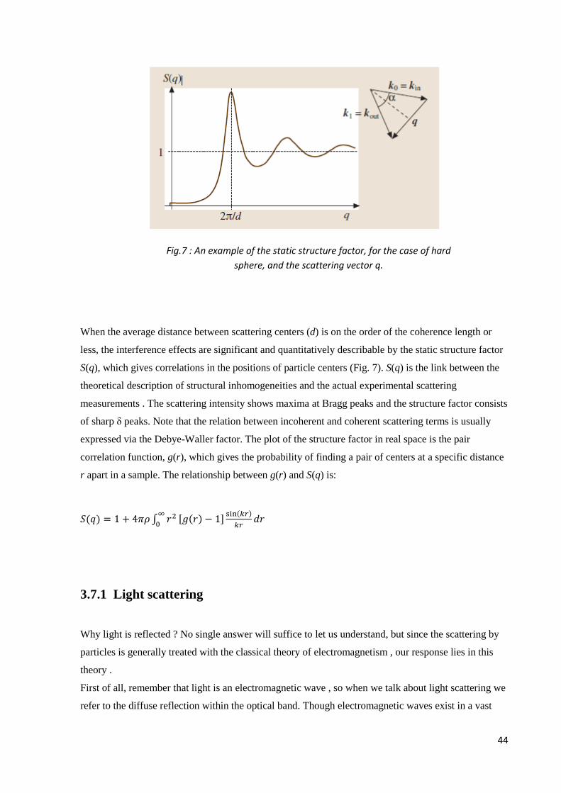
44
When the average distance between scattering centers (d) is on the order of the coherence length or
less, the interference effects are significant and quantitatively describable by the static structure factor
S(q), which gives correlations in the positions of particle centers (Fig. 7). S(q) is the link between the
theoretical description of structural inhomogeneities and the actual experimental scattering
measurements . The scattering intensity shows maxima at Bragg peaks and the structure factor consists
of sharp δ peaks. Note that the relation between incoherent and coherent scattering terms is usually
expressed via the Debye-Waller factor. The plot of the structure factor in real space is the pair
correlation function, g(r), which gives the probability of finding a pair of centers at a specific distance
r apart in a sample. The relationship between g(r) and S(q) is:
3.7.1 Light scattering
Why light is reflected ? No single answer will suffice to let us understand, but since the scattering by
particles is generally treated with the classical theory of electromagnetism , our response lies in this
theory .
First of all, remember that light is an electromagnetic wave , so when we talk about light scattering we
refer to the diffuse reflection within the optical band. Though electromagnetic waves exist in a vast
Fig.7 : An example of the static structure factor, for the case of hard
sphere, and the scattering vector q.
45
range of wavelengths, our eyes are sensitive to only a very narrow band. Since this narrow band of
wavelengths is the means by which humans see, we refer to it as the visible light spectrum.
Although the tangible matter may appear continuous and is often electrically neutral , it is composed
of discrete electric charges . If an obstacle ( interface - plan - a molecule, a single atom or an electron )
is illuminated by the light, which is an electromagnetic wave oscillating, electrical charges within it
are set in motion by the electric field . The charges begin to oscillate and radiate energy in the form of
electromagnetic waves in all directions . In this way, we see a superposition of incident and scattered
waves. The waves radiated from the obstacle are a secondary radiation and are called diffuse radiation
or scattering .
If the particles obey Hooke's law, the oscillation will have the same frequency of the primary wave,
and its amplitude will be significantly weakened. Even the phase will be different and this is because
the speed of light changes when it is in a medium or in free space.
Indeed the individual molecules that constitute matter, diffuse a certain part of the light impinging on
them, and the resulting wave interferes with the primary one, producing a change in the phase which is
equivalent to an wave speed alteration.
If the frequency of the secondary wave is approximately equal to that of the incident wave , we talk of
waves elastically scattered ( sometimes even waves coherently scattered ) or elastic scattering .
Most of the objects are visible thanks to light dispersion from their surfaces , the phenomenon that is
our primary mechanism of physical observation . [14][15]
3.7.2 Types of scattering
In addition to an initial distinction between mixed and single scattering, we can identify different types
of optical diffusion based on different aspects of electromagnetic scattering.
The Mie scattering and Rayleigh scattering are examples of optical elastic, inelastic includes Brillouin
scattering, Raman and Compton (regarding the X-rays).
3.7.3 Rayleigh scattering
Rayleigh scattering (named after the British physicist Lord Rayleigh) is the elastic
scattering of light or other electromagnetic radiation by particles much smaller than the wavelength of
the light (one order of magnitude), which may be individual atoms or molecules.
46
The size of a scattering particle is parametrized by the ratio x of its characteristic dimension r and
wavelength λ:
rx
2
Rayleigh scattering can be defined as scattering in the small size parameter regime x ≪ 1. Scattering
from larger spherical particles is explained by the Mie theory for an arbitrary size parameter x. For
small x the Mie theory reduces to the Rayleigh approximation. In the visible spectrum r must be
smaller of 400nm, minimum wavelength (violet color) and in particular about one tenth of it. Indeed,
if the white light incident on the particles is sufficiently small (≈ 40 nm) the diffused light has always
blue color.
The amount of Rayleigh scattering that occurs for a beam of light is dependent upon the size of the
particles and the wavelength of the light. Specifically, the intensity of the scattered light varies as the
sixth power of the particle size and varies inversely with the fourth power of the wavelength.
Rayleigh scatter α 1/λ4 eq. 5
The intensity I of light scattered by a single small particle from a beam of unpolarized light of
wavelength λ and intensity I0 is given by:
62
2
24
2
2
0 )2
()2
1()
2(
2
cos1 d
n
n
RII
where R is the distance to the particle, θ is the scattering angle, n is the refractive index of the particle,
and d is the diameter of the particle.
Rayleigh scattering cross-section is given by:
(da mc grow hill) This inverse forth power dependencies on wavelength explain why blue light is
scattered more than red light. Consider white light incident on the Earth’s atmosphere. Blue light is
scattered more by the atmosphere than red light. From Eq. 5 we find that blue light at 450 nm scatters
4.4 times more than red light at 650 nm. Without the atmosphere, the sky would appear black during
the daytime, just as was observed by astronauts on the surface of the moon. On Earth, the blue
component of white light is scattered across the atmosphere, which is why the sky is blue!
Furthermore, as the sun falls low on the horizon, the amount of atmosphere through which the sun’s
rays pass increases. This increases the amount of scattering, especially of the shorter wavelengths.
47
With a greater loss of shorter wavelengths, the observer’s perception is that the sun becomes more red;
in actuality it is becoming less blue. This explains why the sun turns increasingly orange and through
to red during a sunset.
3.7.4 Mie scattering
Light scattering caused by objects which are large compared to the wavelength of light is known as
Mie scattering. Generally speaking, Mie scattering becomes significant when the scattering particle is
larger than approximately 1/10th of the wavelength of light. Mie scattering theory is a general theory
for scattering caused by any diameter of spherical particle. Mie scattering is particularly useful for
colloids. This is a key form of scattering in optical fiber communications, where scattering must be
minimized along long lengths of optical fiber to achieve good communication distances.
3.7.5 Brillouin scattering
When light propagating in a medium (air, water, crystals…) interacts with time- dependent optical
density variations can undergo a collision (usually inelastic) and change its energy (frequency) and
path. This type of collision is called Brillouin scattering.
From a strictly classical point of view, the compression of the medium will change the index of
refraction and therefore lead to some reflection or scattering at any point where the index changes.
From a quantum point of view, the process can be considered one of interaction of light photons with
acoustic or vibrational quanta (phonons. These are a quantum of energy or a quasi-particle associated
with a compressional wave such as sound or a vibration of a crystal lattice).
When acoustic standing waves are produced in a solid, they create a periodic condition which can
scatter light waves according to the Bragg law. In addition to its application to X-ray diffraction, the
Bragg law applies to some cases of light scattering from acoustic standing wave modes in a solid. This
is an example of Brillouin scattering.
3.7.6 Raman scattering
Raman effect (discovered by CV Raman in 1928) is an example of inelastic scattering, more precisely
a collision in which the particles interacting exchange energy. (e.i. Chromatic passage). In Raman
scattering an incident photon on a molecule can lose energy to create a quantum fluctuation or may
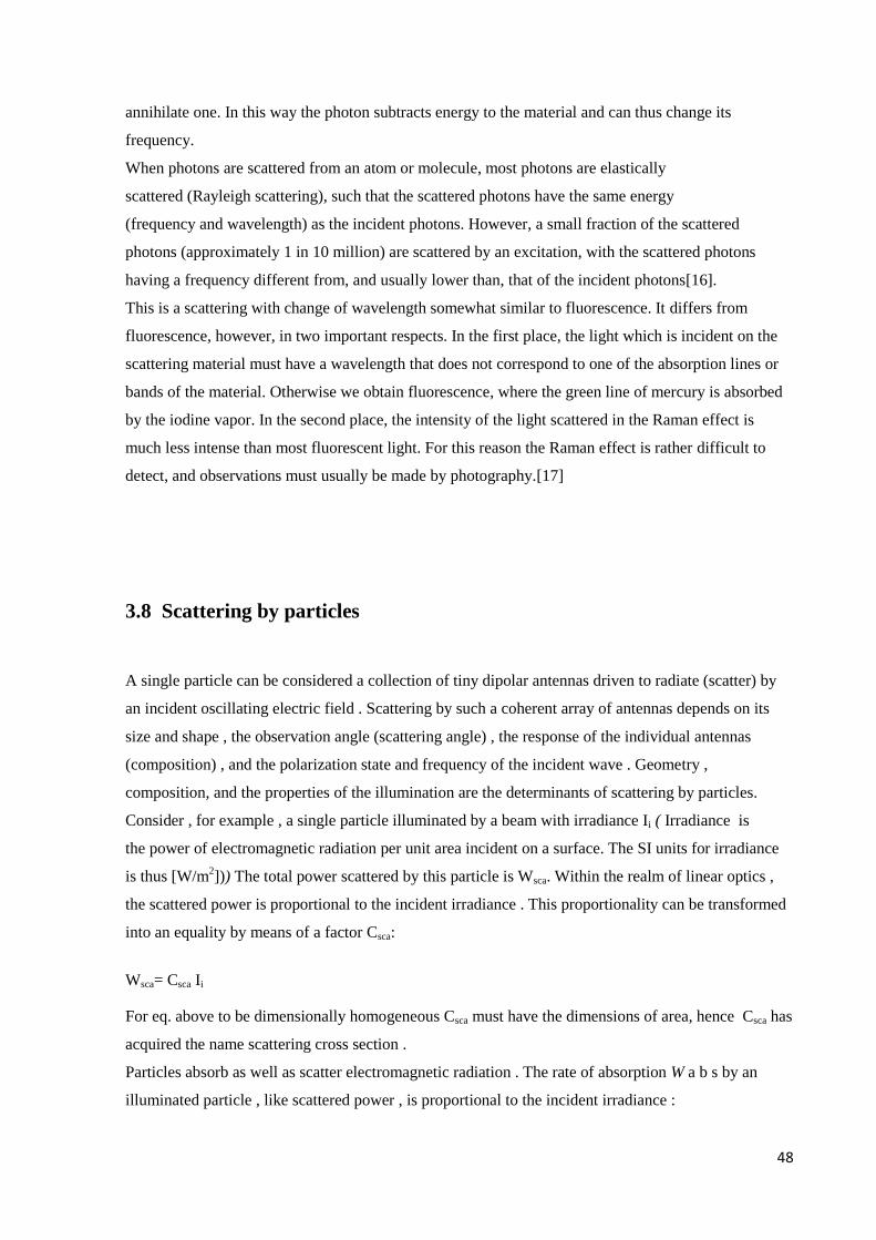
48
annihilate one. In this way the photon subtracts energy to the material and can thus change its
frequency.
When photons are scattered from an atom or molecule, most photons are elastically
scattered (Rayleigh scattering), such that the scattered photons have the same energy
(frequency and wavelength) as the incident photons. However, a small fraction of the scattered
photons (approximately 1 in 10 million) are scattered by an excitation, with the scattered photons
having a frequency different from, and usually lower than, that of the incident photons[16].
This is a scattering with change of wavelength somewhat similar to fluorescence. It differs from
fluorescence, however, in two important respects. In the first place, the light which is incident on the
scattering material must have a wavelength that does not correspond to one of the absorption lines or
bands of the material. Otherwise we obtain fluorescence, where the green line of mercury is absorbed
by the iodine vapor. In the second place, the intensity of the light scattered in the Raman effect is
much less intense than most fluorescent light. For this reason the Raman effect is rather difficult to
detect, and observations must usually be made by photography.[17]
3.8 Scattering by particles
A single particle can be considered a collection of tiny dipolar antennas driven to radiate (scatter) by
an incident oscillating electric field . Scattering by such a coherent array of antennas depends on its
size and shape , the observation angle (scattering angle) , the response of the individual antennas
(composition) , and the polarization state and frequency of the incident wave . Geometry ,
composition, and the properties of the illumination are the determinants of scattering by particles.
Consider , for example , a single particle illuminated by a beam with irradiance Ii ( Irradiance is
the power of electromagnetic radiation per unit area incident on a surface. The SI units for irradiance
is thus [W/m2])) The total power scattered by this particle is Wsca. Within the realm of linear optics ,
the scattered power is proportional to the incident irradiance . This proportionality can be transformed
into an equality by means of a factor Csca:
Wsca= Csca Ii
For eq. above to be dimensionally homogeneous Csca must have the dimensions of area, hence Csca has
acquired the name scattering cross section .
Particles absorb as well as scatter electromagnetic radiation . The rate of absorption W a b s by an
illuminated particle , like scattered power , is proportional to the incident irradiance :
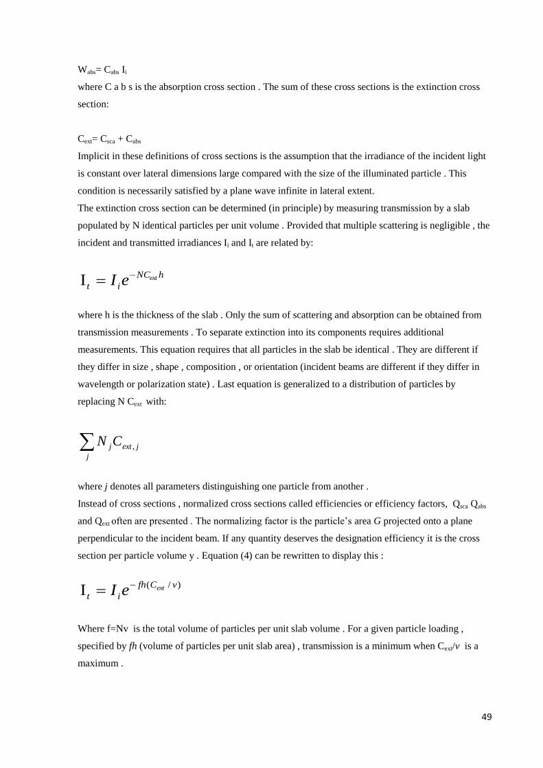
49
Wabs= Cabs Ii
where C a b s is the absorption cross section . The sum of these cross sections is the extinction cross
section:
Cext= Csca + Cabs
Implicit in these definitions of cross sections is the assumption that the irradiance of the incident light
is constant over lateral dimensions large compared with the size of the illuminated particle . This
condition is necessarily satisfied by a plane wave infinite in lateral extent.
The extinction cross section can be determined (in principle) by measuring transmission by a slab
populated by N identical particles per unit volume . Provided that multiple scattering is negligible , the
incident and transmitted irradiances Ii and It are related by:
hNC
itexteI
I
where h is the thickness of the slab . Only the sum of scattering and absorption can be obtained from
transmission measurements . To separate extinction into its components requires additional
measurements. This equation requires that all particles in the slab be identical . They are different if
they differ in size , shape , composition , or orientation (incident beams are different if they differ in
wavelength or polarization state) . Last equation is generalized to a distribution of particles by
replacing N Cext with:
j
jextjCN ,
where j denotes all parameters distinguishing one particle from another .
Instead of cross sections , normalized cross sections called efficiencies or efficiency factors, Qsca Qabs
and Qext often are presented . The normalizing factor is the particle’s area G projected onto a plane
perpendicular to the incident beam. If any quantity deserves the designation efficiency it is the cross
section per particle volume y . Equation (4) can be rewritten to display this :
)/(I
vCfh
itexteI
Where f=Nv is the total volume of particles per unit slab volume . For a given particle loading ,
specified by fh (volume of particles per unit slab area) , transmission is a minimum when Cext/v is a
maximum .
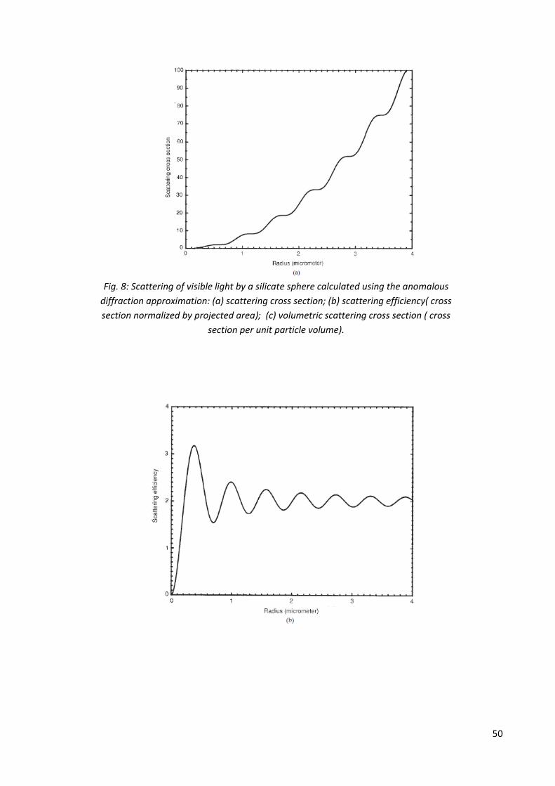
50
Fig. 8: Scattering of visible light by a silicate sphere calculated using the anomalous
diffraction approximation: (a) scattering cross section; (b) scattering efficiency( cross
section normalized by projected area); (c) volumetric scattering cross section ( cross
section per unit particle volume).
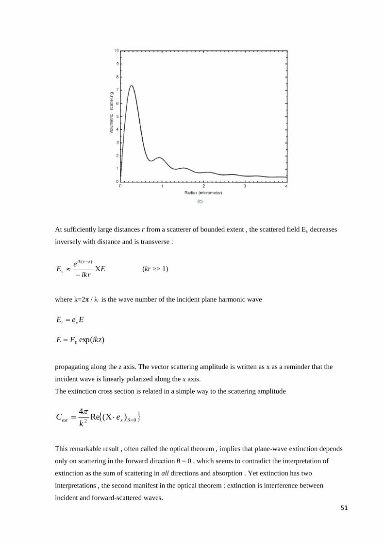
51
At sufficiently large distances r from a scatterer of bounded extent , the scattered field Es decreases
inversely with distance and is transverse :
Eikr
eE
zrik
s
)(
(kr >> 1)
where k=2π / λ is the wave number of the incident plane harmonic wave
EeE xi
)exp(0 ikzEE
propagating along the z axis. The vector scattering amplitude is written as x as a reminder that the
incident wave is linearly polarized along the x axis.
The extinction cross section is related in a simple way to the scattering amplitude
02)(Re
4
xext e
kC
This remarkable result , often called the optical theorem , implies that plane-wave extinction depends
only on scattering in the forward direction θ = 0 , which seems to contradict the interpretation of
extinction as the sum of scattering in all directions and absorption . Yet extinction has two
interpretations , the second manifest in the optical theorem : extinction is interference between
incident and forward-scattered waves.
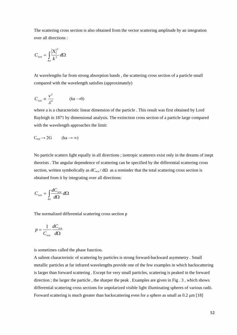
52
The scattering cross section is also obtained from the vector scattering amplitude by an integration
over all directions :
4
2
2
dk
Csca
At wavelengths far from strong absorption bands , the scattering cross section of a particle small
compared with the wavelength satisfies (approximately)
4
2
vCsca (ka →0)
where a is a characteristic linear dimension of the particle . This result was first obtained by Lord
Rayleigh in 1871 by dimensional analysis. The extinction cross section of a particle large compared
with the wavelength approaches the limit:
Cext → 2G (ka → ∞)
No particle scatters light equally in all directions ; isotropic scatterers exist only in the dreams of inept
theorists . The angular dependence of scattering can be specified by the differential scattering cross
section, written symbolically as dCsca / dΩ as a reminder that the total scattering cross section is
obtained from it by integrating over all directions:
4
dd
dCC sca
sca
The normalized differential scattering cross section p
d
dC
Cp sca
sca
1
is sometimes called the phase function.
A salient characteristic of scattering by particles is strong forward-backward asymmetry . Small
metallic particles at far infrared wavelengths provide one of the few examples in which backscattering
is larger than forward scattering . Except for very small particles, scattering is peaked in the forward
direction ; the larger the particle , the sharper the peak . Examples are given in Fig . 3 , which shows
differential scattering cross sections for unpolarized visible light illuminating spheres of various radii.
Forward scattering is much greater than backscattering even for a sphere as small as 0.2 μm [18]
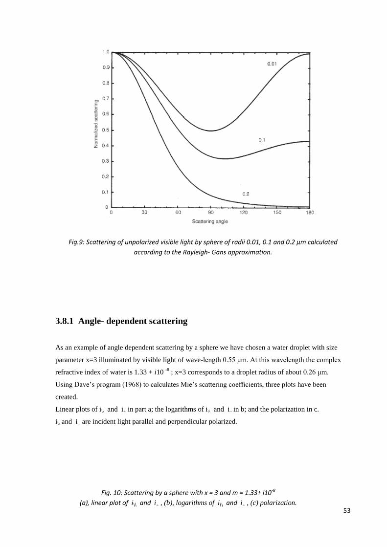
53
3.8.1 Angle- dependent scattering
As an example of angle dependent scattering by a sphere we have chosen a water droplet with size
parameter x=3 illuminated by visible light of wave-length 0.55 μm. At this wavelength the complex
refractive index of water is 1.33 + i10 -8
; x=3 corresponds to a droplet radius of about 0.26 μm.
Using Dave’s program (1968) to calculates Mie’s scattering coefficients, three plots have been
created.
Linear plots of i\\ and i+ in part a; the logarithms of i\\ and i+ in b; and the polarization in c.
i\\ and i+ are incident light parallel and perpendicular polarized.
Fig.9: Scattering of unpolarized visible light by sphere of radii 0.01, 0.1 and 0.2 μm calculated
according to the Rayleigh- Gans approximation.
Fig. 10: Scattering by a sphere with x = 3 and m = 1.33+ i10-8
(a), linear plot of i\\ and i+ , (b), logarithms of i\\ and i+ , (c) polarization.
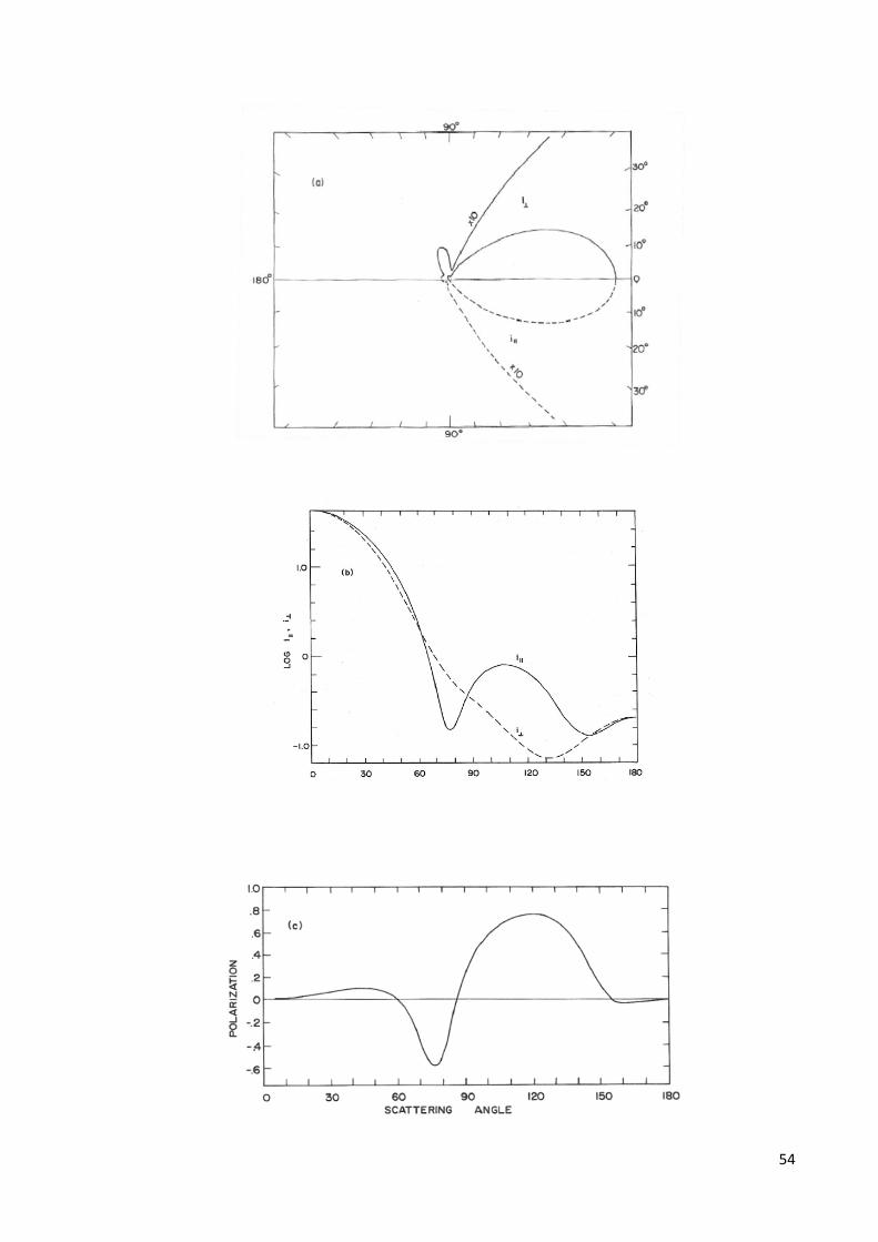
54
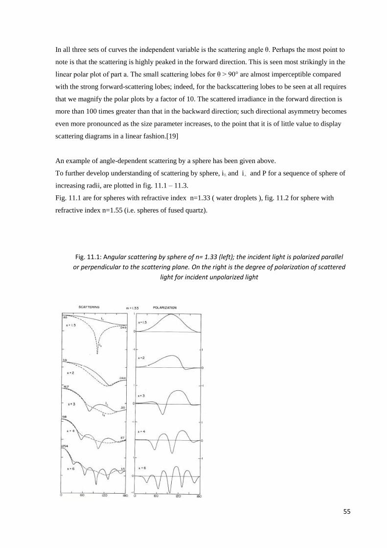
55
In all three sets of curves the independent variable is the scattering angle θ. Perhaps the most point to
note is that the scattering is highly peaked in the forward direction. This is seen most strikingly in the
linear polar plot of part a. The small scattering lobes for θ > 90° are almost imperceptible compared
with the strong forward-scattering lobes; indeed, for the backscattering lobes to be seen at all requires
that we magnify the polar plots by a factor of 10. The scattered irradiance in the forward direction is
more than 100 times greater than that in the backward direction; such directional asymmetry becomes
even more pronounced as the size parameter increases, to the point that it is of little value to display
scattering diagrams in a linear fashion.[19]
An example of angle-dependent scattering by a sphere has been given above.
To further develop understanding of scattering by sphere, i\\ and i+ and P for a sequence of sphere of
increasing radii, are plotted in fig. 11.1 – 11.3.
Fig. 11.1 are for spheres with refractive index n=1.33 ( water droplets ), fig. 11.2 for sphere with
refractive index n=1.55 (i.e. spheres of fused quartz).
Fig. 11.1: Angular scattering by sphere of n= 1.33 (left); the incident light is polarized parallel
or perpendicular to the scattering plane. On the right is the degree of polarization of scattered
light for incident unpolarized light
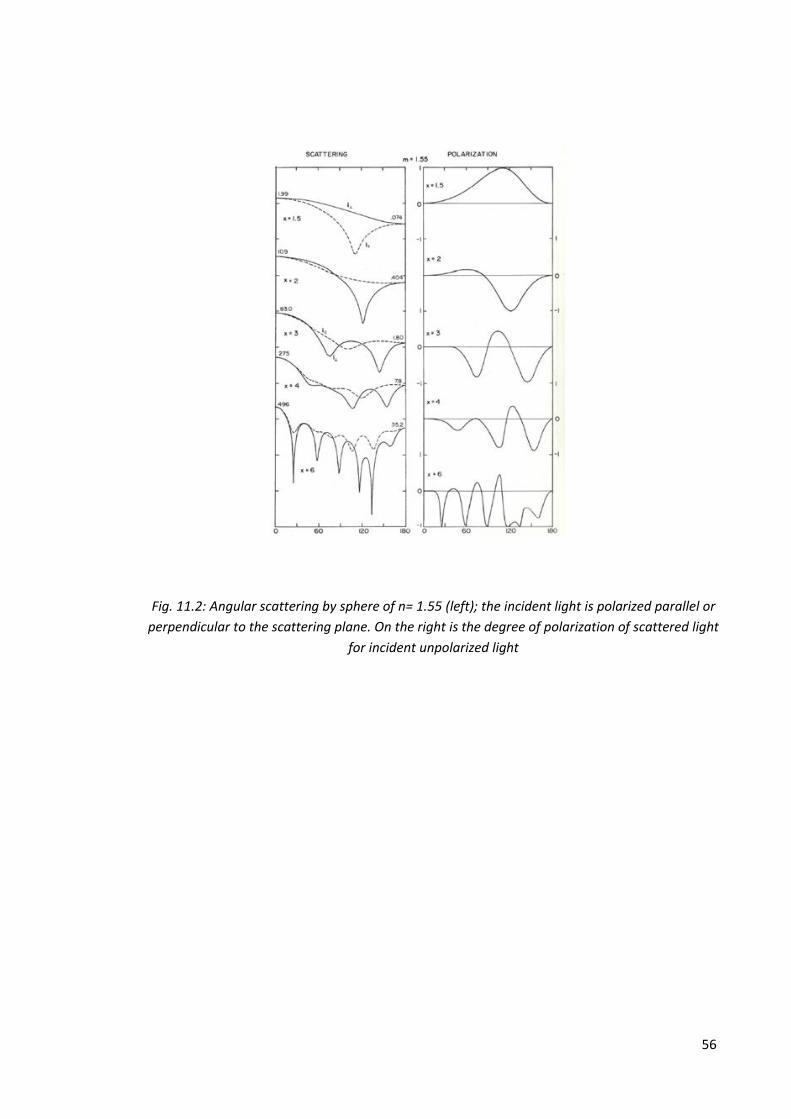
56
Fig. 11.2: Angular scattering by sphere of n= 1.55 (left); the incident light is polarized parallel or
perpendicular to the scattering plane. On the right is the degree of polarization of scattered light
for incident unpolarized light
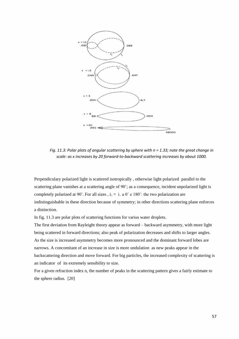
57
Perpendiculary polarized light is scattered isotropically , otherwise light polarized parallel to the
scattering plane vanishes at a scattering angle of 90˚; as a consequence, incident unpolarized light is
completely polarized at 90˚. For all sizes , i\\ = i+ a 0˚ e 180˚: the two polarization are
indistinguishable in these direction because of symmetry; in other directions scattering plane enforces
a distinction.
In fig. 11.3 are polar plots of scattering functions for varius water droplets.
The first deviation from Rayleight theory appear as forward – backward asymmetry, with more light
being scattered in forward directions; also peak of polarization decreases and shifts to larger angles.
As the size is increased asymmetry becomes more pronounced and the dominant forward lobes are
narrows. A concomitant of an increase in size is more undulation as new peaks appear in the
backscattering direction and move forward. For big particles, the increased complexity of scattering is
an indicator of its extremely sensibility to size.
For a given refraction index n, the number of peaks in the scattering pattern gives a fairly estimate to
the sphere radius. [20]
Fig. 11.3: Polar plots of angular scattering by sphere with n = 1.33; note the great change in
scale: as x increases by 20 forward-to-backward scattering increases by about 1000.
58
References
[1] [2] “Liquid crystals, laptops and life”. Michael R. Fisch,
[3] “Appunti di campi elettromagnetici” , G. Manara, A. Monorchio , P. Nepa
[4] “Modern optical engineering”, W. Smith, McGraw Hill Professional
[5] Enciclopedia della scienza e della tecnica, Treccani, 2008
[6] Wikipedia, http://en.wikipedia.org/wiki/Elastic_scattering
[9) “Handbook of laser and optics”, Springer, 1st ed. 2007
[7] [8] [10] Appunti tratti dalle lezioni di Fenomeni Bioelettrici.
[11] Wikipedia e web, http://en.wikipedia.org/wiki/Scattering
[12] “ Physics Quick Study Guide for Smartphones and Mobile Devices”, from MobileReference,
[13] “Handbook of laser and optics”, Springer, 1st ed. 2007
[14] “The Scattering of Light”, Kerker, M. (1969), New York: Academic. ISBN 0-12-404550-2.
[15] "Light Scattering by Inhomogeneous Media". Mandelstam, L.I. (1926). Zh. Russ. Fiz-Khim
[16] “Symmetry and Spectroscopy”, Harris and Bertolucci (1989), Dover Publications. ISBN 0-486-
66144-X.)
[17] ,“Fundamentals of scattering”, Michael Francis A. Jenkins & Harvey E McGraw-Hill 1957
[18] “Handbook of laser and optics”, Springer, 1st ed. 2007 [Volume I_Scattering, Craig F.Bohren]
[19] [20] “Absorption and scattering of light by small particles ”, C.F. Bohren, Wiley 2004.
59
Chapter 4
TUNEABLE OPTICAL FILTER: PROPOSED
EVALUATION SYSTEM
As mentioned before, several approaches had been proposed to simulate the natural vision though log-
polar imaging. It consists of a methods that represents visual information with a space-variant
resolution inspired by the visual system of mammals. This can be reached with physical or
computational solutions.
Sandini’s paper [1] proposes a retina-like sensor characterized by a space-variant resolution similar to
that of the human retina. This implementation is called log-polar structure and consists of a constant
number of photosites arranged over concentric rings (the polar part of the representation) giving rise to
a linear increase of the receptor's spacing with respect to the distance from the central point of the
structure The realization of such a device uses a CMOS technology with sensor of a constant
dimension of 0.35 μ m.
Compared with the first realization where the sensor dimension was ten times bigger, it was possible
to have a better coverage of the central part. However the dimensions remain constant. Thus such a
device has the main limit in the central area, exactly where resolution should be maximum, because is
not completely covered by sensors.
In computational approaches we remember Zoujing paper [2]. He proposes a new computational
method to simulate distribution of retina photoreceptors implementing a low bandwidth method using
Gaussian multi-resolution pyramids (filters). A constant resolution image had been decomposed in
sub-images, called pyramidal levels, characterized by a lower information content.
In order to apply the foveation framework described above to image compressing, they conceive a
standard framework for transmitting the necessary data. In addition to the pyramid encoding, the
image data had been compressed before transmission using some linear encoding mechanism such as
Huffman coding.
Such a methodology is limited by the rate of transmission through a common wi-fi network and has a
not negligible computational complexity in terms of development of the entire pyramidal structure
and in data transmission.
60
Differently we are looking for a tuneable optical response upon an electrical stimulation so as to
attenuate spatial frequencies before the photodetector sampling. Our approach is based on the
phenomenon of light scattering to filter the input light signal physically. This to avoid computational
complexity of a software method and to have a simpler device compared to the one using CMOS
sensors, where small sensor are still difficult to place in the central area.
4.1 System description
The aim of this work is to approach the designing of an electrically tuneable optical filter based on
light scattering phenomenon (within the visible spectrum of wavelengths 400 - 700 nm) in order to
mimic the foveal vision in human eyes.
As seen in chapter 2 light rays are focused onto the retina through our cornea, pupil and lens. The
retina converts the light rays into electrical signals which travel through the optic nerve to our brain,
where they are interpreted as the images we see.
The retina is a layered structure with several layers of neurons interconnected by synapses. The only
neurons that are directly sensitive to light are the photoreceptor cells, the rods and cones.
We have surprisingly low visual acuity (resolution) in parts of the visual field that are not at the center
of gaze - where we are looking. We are not aware of this because we instinctively direct our center of
gaze to where we are looking. The center of gaze, called the fovea, has a higher density of cones than
anywhere else on the retina. In fact, at the fovea, there are no rods at all. (In the diagram at right, the
cones are shown in green.) The fovea evolved to have the highest possible visual acuity, and the cones
are as small as they can possibly be and still function. For this reason the image that we perceive is
sharp in the centre o in the point of gaze and incrementally blurred towards the periphery.
The fact that our vision has the highest acuity in the center of gaze does not mean that our vision in
the rest of the visual field is inferior — it’s simply used for different things. Foveal vision is used for
scrutinizing highly detailed objects, whereas peripheral vision is used for organizing the broad spatial
scene and for seeing large objects. Our foveal vision is optimized for fine details, and our peripheral
vision is optimized for coarser information.
Where are more cone photoreceptors, there is more frequency information of the objects and the
cleaner the image on the retina vise versa. the spatial resolution is not constant across our field of
view, but is maximal at the fovea. Thanks to the eye movement objects placed in all areas of the space
can be perceived with sharpness. Indeed, the image created in our mind is always much sharper in a
neighborhood of the gaze point and appears blurred in the surrounding area.
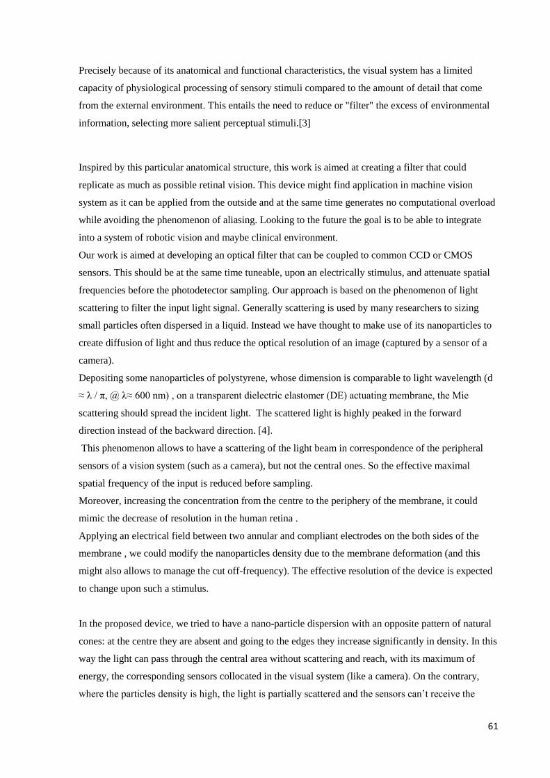
61
Precisely because of its anatomical and functional characteristics, the visual system has a limited
capacity of physiological processing of sensory stimuli compared to the amount of detail that come
from the external environment. This entails the need to reduce or "filter" the excess of environmental
information, selecting more salient perceptual stimuli.[3]
Inspired by this particular anatomical structure, this work is aimed at creating a filter that could
replicate as much as possible retinal vision. This device might find application in machine vision
system as it can be applied from the outside and at the same time generates no computational overload
while avoiding the phenomenon of aliasing. Looking to the future the goal is to be able to integrate
into a system of robotic vision and maybe clinical environment.
Our work is aimed at developing an optical filter that can be coupled to common CCD or CMOS
sensors. This should be at the same time tuneable, upon an electrically stimulus, and attenuate spatial
frequencies before the photodetector sampling. Our approach is based on the phenomenon of light
scattering to filter the input light signal. Generally scattering is used by many researchers to sizing
small particles often dispersed in a liquid. Instead we have thought to make use of its nanoparticles to
create diffusion of light and thus reduce the optical resolution of an image (captured by a sensor of a
camera).
Depositing some nanoparticles of polystyrene, whose dimension is comparable to light wavelength (d
≈ λ / π, @ λ≈ 600 nm) , on a transparent dielectric elastomer (DE) actuating membrane, the Mie
scattering should spread the incident light. The scattered light is highly peaked in the forward
direction instead of the backward direction. [4].
This phenomenon allows to have a scattering of the light beam in correspondence of the peripheral
sensors of a vision system (such as a camera), but not the central ones. So the effective maximal
spatial frequency of the input is reduced before sampling.
Moreover, increasing the concentration from the centre to the periphery of the membrane, it could
mimic the decrease of resolution in the human retina .
Applying an electrical field between two annular and compliant electrodes on the both sides of the
membrane , we could modify the nanoparticles density due to the membrane deformation (and this
might also allows to manage the cut off-frequency). The effective resolution of the device is expected
to change upon such a stimulus.
In the proposed device, we tried to have a nano-particle dispersion with an opposite pattern of natural
cones: at the centre they are absent and going to the edges they increase significantly in density. In this
way the light can pass through the central area without scattering and reach, with its maximum of
energy, the corresponding sensors collocated in the visual system (like a camera). On the contrary,
where the particles density is high, the light is partially scattered and the sensors can’t receive the
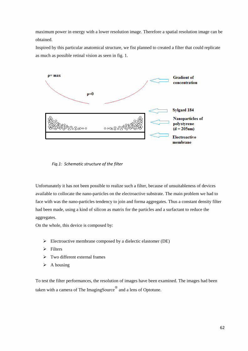
62
maximum power in energy with a lower resolution image. Therefore a spatial resolution image can be
obtained.
Inspired by this particular anatomical structure, we fist planned to created a filter that could replicate
as much as possible retinal vision as seen in fig. 1.
Unfortunately it has not been possible to realize such a filter, because of unsuitableness of devices
available to collocate the nano-particles on the electroactive substrate. The main problem we had to
face with was the nano-particles tendency to join and forma aggregates. Thus a constant density filter
had been made, using a kind of silicon as matrix for the particles and a surfactant to reduce the
aggregates.
On the whole, this device is composed by:
Electroactive membrane composed by a dielectic elastomer (DE)
Filters
Two different external frames
A housing
To test the filter performances, the resolution of images have been examined. The images had been
taken with a camera of The ImagingSource®
and a lens of Optotune.
Fig.1: Schematic structure of the filter
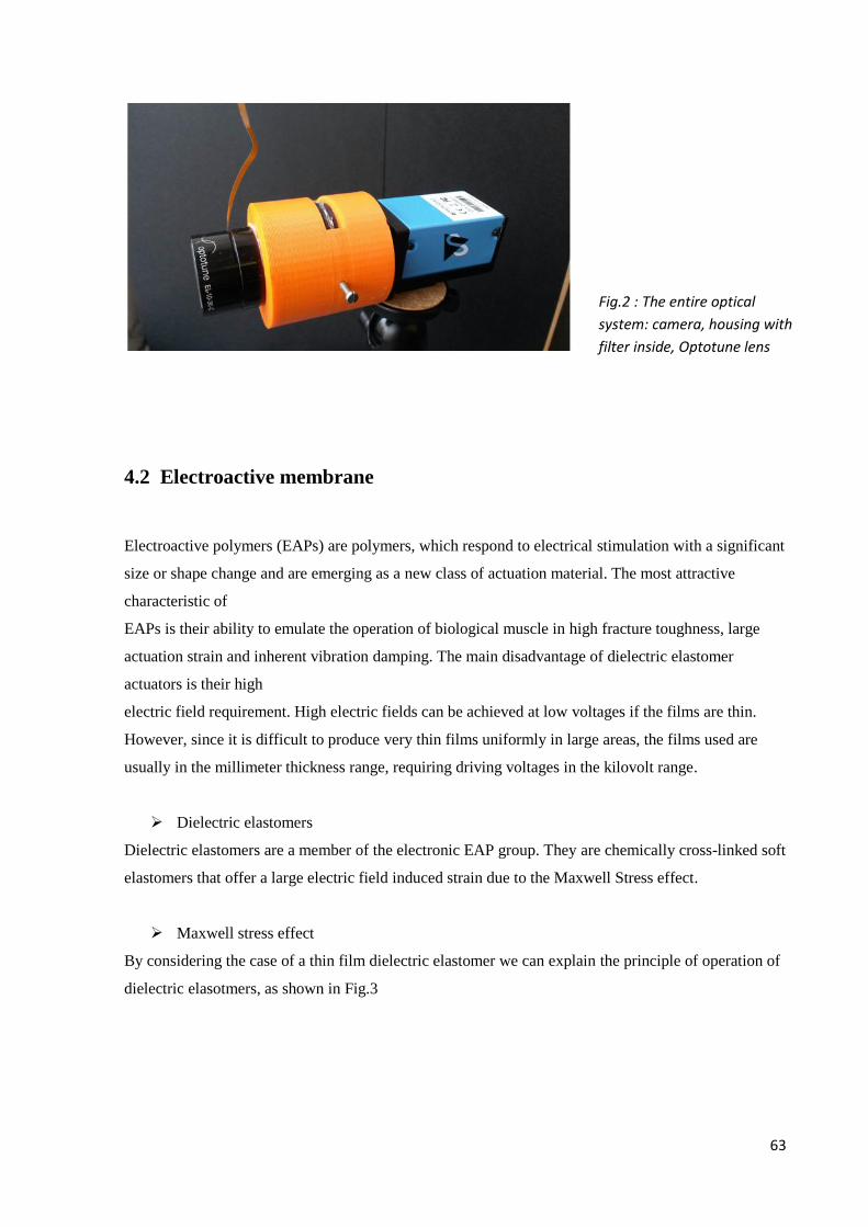
63
4.2 Electroactive membrane
Electroactive polymers (EAPs) are polymers, which respond to electrical stimulation with a significant
size or shape change and are emerging as a new class of actuation material. The most attractive
characteristic of
EAPs is their ability to emulate the operation of biological muscle in high fracture toughness, large
actuation strain and inherent vibration damping. The main disadvantage of dielectric elastomer
actuators is their high
electric field requirement. High electric fields can be achieved at low voltages if the films are thin.
However, since it is difficult to produce very thin films uniformly in large areas, the films used are
usually in the millimeter thickness range, requiring driving voltages in the kilovolt range.
Dielectric elastomers
Dielectric elastomers are a member of the electronic EAP group. They are chemically cross-linked soft
elastomers that offer a large electric field induced strain due to the Maxwell Stress effect.
Maxwell stress effect
By considering the case of a thin film dielectric elastomer we can explain the principle of operation of
dielectric elasotmers, as shown in Fig.3
Fig.2 : The entire optical
system: camera, housing with
filter inside, Optotune lens
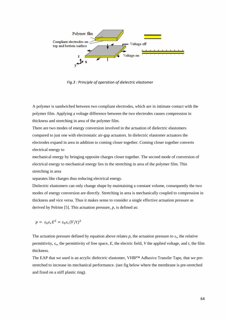
64
A polymer is sandwiched between two compliant electrodes, which are in intimate contact with the
polymer film. Applying a voltage difference between the two electrodes causes compression in
thickness and stretching in area of the polymer film.
There are two modes of energy conversion involved in the actuation of dielectric elastomers
compared to just one with electrostatic air-gap actuators. In dielectric elastomer actuators the
electrodes expand in area in addition to coming closer together. Coming closer together converts
electrical energy to
mechanical energy by bringing opposite charges closer together. The second mode of conversion of
electrical energy to mechanical energy lies in the stretching in area of the polymer film. This
stretching in area
separates like charges thus reducing electrical energy.
Dielectric elastomers can only change shape by maintaining a constant volume, consequently the two
modes of energy conversion are directly. Stretching in area is mechanically coupled to compression in
thickness and vice versa. Thus it makes sense to consider a single effective actuation pressure as
derived by Pelrine [5]. This actuation pressure, p, is defined as:
The actuation pressure defined by equation above relates p, the actuation pressure to εr, the relative
permittivity, εo, the permittivity of free space, E, the electric field, V the applied voltage, and t, the film
thickness.
The EAP that we used is an acrylic dielectric elastomer, VHB™ Adhesive Transfer Tape, that we pre-
stretched to increase its mechanical performance. (see fig below where the membrane is pre-stretched
and fixed on a stiff plastic ring).
Fig.3 : Principle of operation of dielectric elastomer
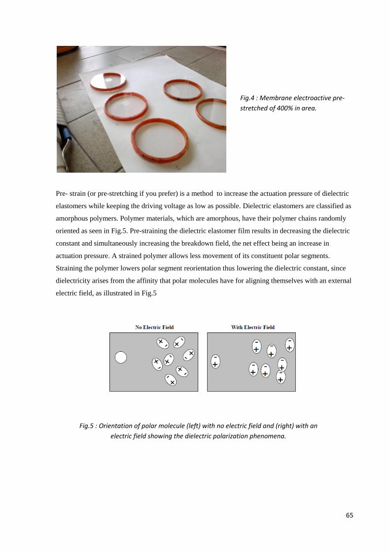
65
Pre- strain (or pre-stretching if you prefer) is a method to increase the actuation pressure of dielectric
elastomers while keeping the driving voltage as low as possible. Dielectric elastomers are classified as
amorphous polymers. Polymer materials, which are amorphous, have their polymer chains randomly
oriented as seen in Fig.5. Pre-straining the dielectric elastomer film results in decreasing the dielectric
constant and simultaneously increasing the breakdown field, the net effect being an increase in
actuation pressure. A strained polymer allows less movement of its constituent polar segments.
Straining the polymer lowers polar segment reorientation thus lowering the dielectric constant, since
dielectricity arises from the affinity that polar molecules have for aligning themselves with an external
electric field, as illustrated in Fig.5
Fig.4 : Membrane electroactive pre-
stretched of 400% in area.
Fig.5 : Orientation of polar molecule (left) with no electric field and (right) with an
electric field showing the dielectric polarization phenomena.
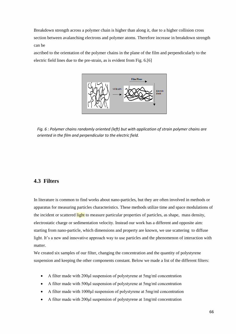
66
Breakdown strength across a polymer chain is higher than along it, due to a higher collision cross
section between avalanching electrons and polymer atoms. Therefore increase in breakdown strength
can be
ascribed to the orientation of the polymer chains in the plane of the film and perpendicularly to the
electric field lines due to the pre-strain, as is evident from Fig. 6.[6]
4.3 Filters
In literature is common to find works about nano-particles, but they are often involved in methods or
apparatus for measuring particles characteristics. These methods utilize time and space modulations of
the incident or scattered light to measure particular properties of particles, as shape, mass density,
electrostatic charge or sedimentation velocity. Instead our work has a different and opposite aim:
starting from nano-particle, which dimensions and property are known, we use scattering to diffuse
light. It’s a new and innovative approach way to use particles and the phenomenon of interaction with
matter.
We created six samples of our filter, changing the concentration and the quantity of polystyrene
suspension and keeping the other components constant. Below we made a list of the different filters:
A filter made with 200μl suspension of polystyrene at 5mg/ml concentration
A filter made with 500μl suspension of polystyrene at 5mg/ml concentration
A filter made with 1000μl suspension of polystyrene at 5mg/ml concentration
A filter made with 200μl suspension of polystyrene at 1mg/ml concentration
Fig. 6 : Polymer chains randomly oriented (left) but with application of strain polymer chains are
oriented in the film and perpendicular to the electric field.
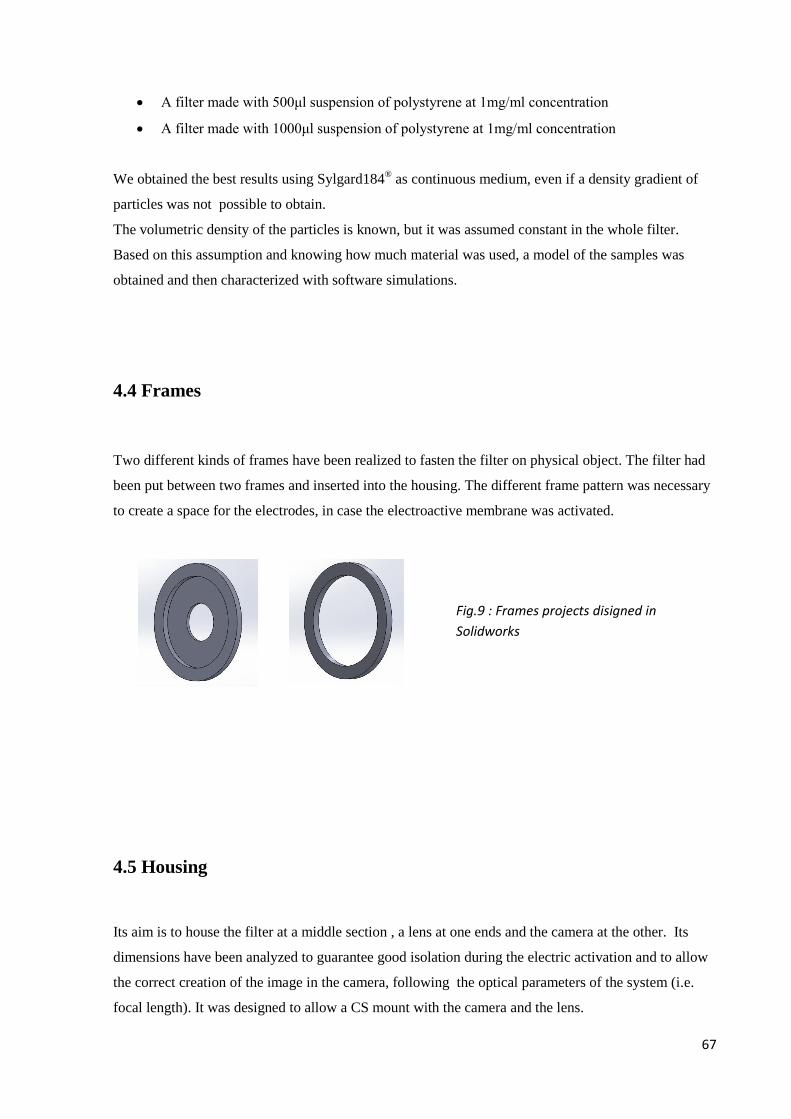
67
A filter made with 500μl suspension of polystyrene at 1mg/ml concentration
A filter made with 1000μl suspension of polystyrene at 1mg/ml concentration
We obtained the best results using Sylgard184® as continuous medium, even if a density gradient of
particles was not possible to obtain.
The volumetric density of the particles is known, but it was assumed constant in the whole filter.
Based on this assumption and knowing how much material was used, a model of the samples was
obtained and then characterized with software simulations.
4.4 Frames
Two different kinds of frames have been realized to fasten the filter on physical object. The filter had
been put between two frames and inserted into the housing. The different frame pattern was necessary
to create a space for the electrodes, in case the electroactive membrane was activated.
4.5 Housing
Its aim is to house the filter at a middle section , a lens at one ends and the camera at the other. Its
dimensions have been analyzed to guarantee good isolation during the electric activation and to allow
the correct creation of the image in the camera, following the optical parameters of the system (i.e.
focal length). It was designed to allow a CS mount with the camera and the lens.
Fig.9 : Frames projects disigned in
Solidworks
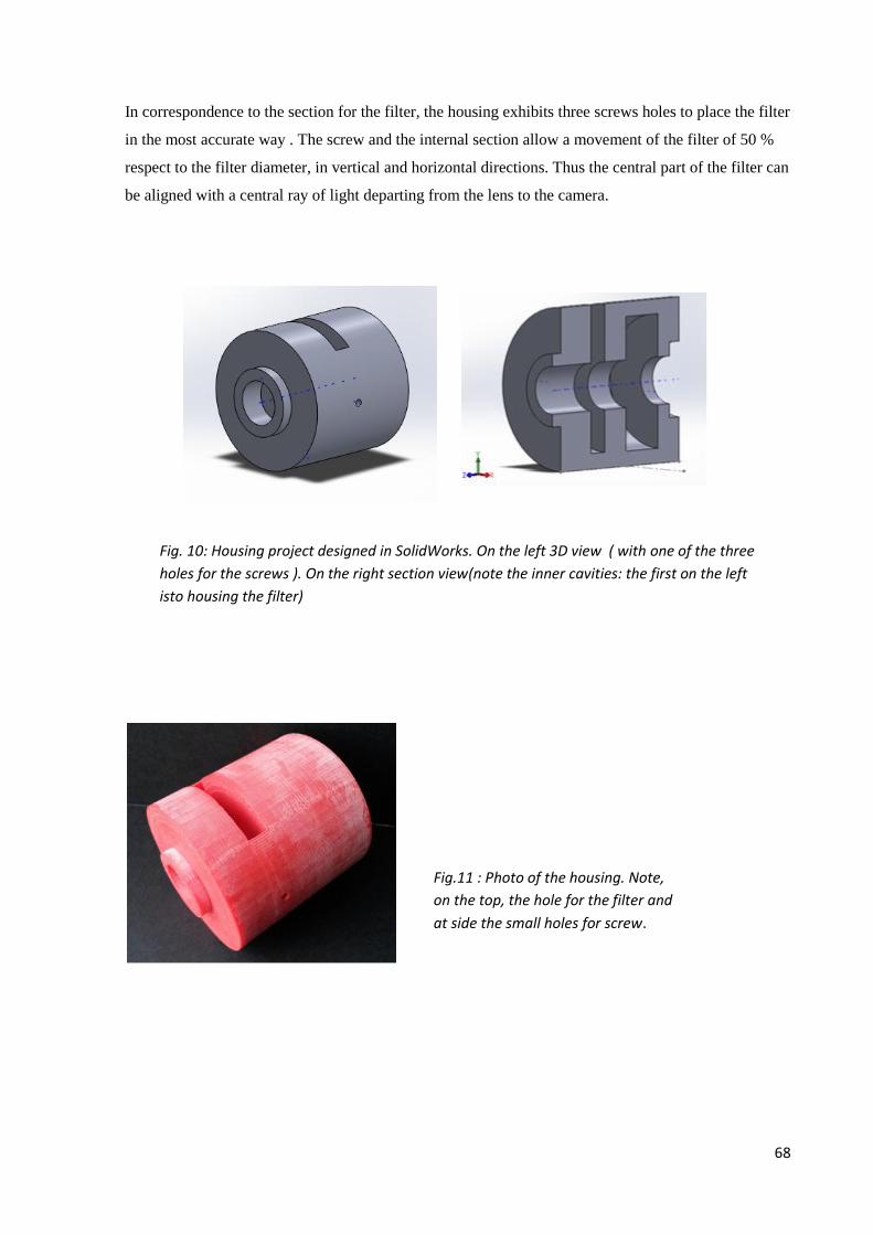
68
In correspondence to the section for the filter, the housing exhibits three screws holes to place the filter
in the most accurate way . The screw and the internal section allow a movement of the filter of 50 %
respect to the filter diameter, in vertical and horizontal directions. Thus the central part of the filter can
be aligned with a central ray of light departing from the lens to the camera.
Fig. 10: Housing project designed in SolidWorks. On the left 3D view ( with one of the three
holes for the screws ). On the right section view(note the inner cavities: the first on the left
isto housing the filter)
Fig.11 : Photo of the housing. Note,
on the top, the hole for the filter and
at side the small holes for screw.
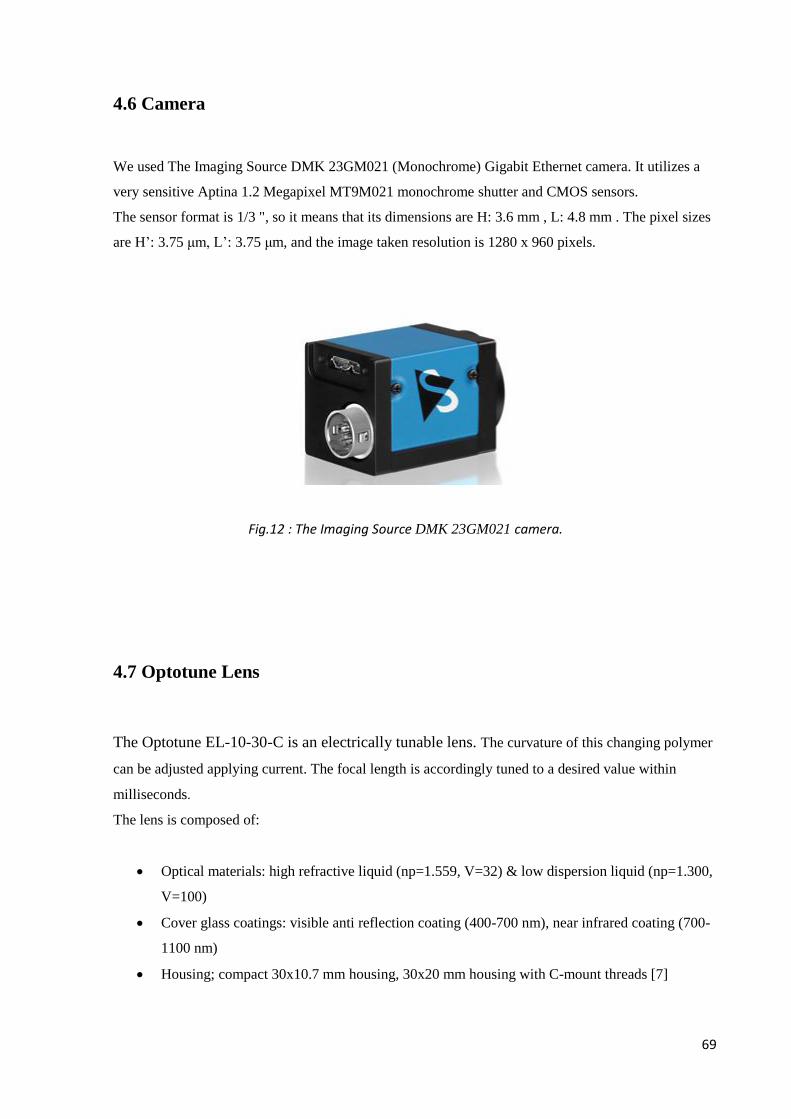
69
4.6 Camera
We used The Imaging Source DMK 23GM021 (Monochrome) Gigabit Ethernet camera. It utilizes a
very sensitive Aptina 1.2 Megapixel MT9M021 monochrome shutter and CMOS sensors.
The sensor format is 1/3 ", so it means that its dimensions are H: 3.6 mm , L: 4.8 mm . The pixel sizes
are H’: 3.75 μm, L’: 3.75 μm, and the image taken resolution is 1280 x 960 pixels.
4.7 Optotune Lens
The Optotune EL-10-30-C is an electrically tunable lens. The curvature of this changing polymer
can be adjusted applying current. The focal length is accordingly tuned to a desired value within
milliseconds.
The lens is composed of:
Optical materials: high refractive liquid (np=1.559, V=32) & low dispersion liquid (np=1.300,
V=100)
Cover glass coatings: visible anti reflection coating (400-700 nm), near infrared coating (700-
1100 nm)
Housing; compact 30x10.7 mm housing, 30x20 mm housing with C-mount threads [7]
Fig.12 : The Imaging Source DMK 23GM021 camera.
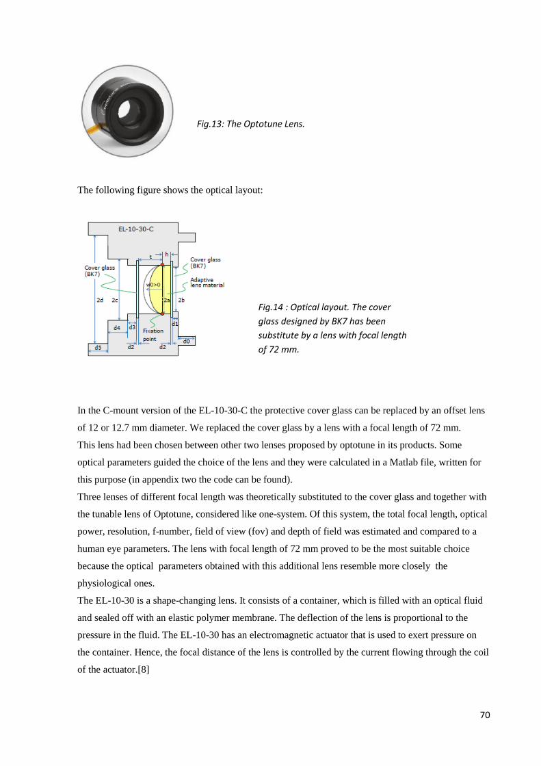
70
The following figure shows the optical layout:
In the C-mount version of the EL-10-30-C the protective cover glass can be replaced by an offset lens
of 12 or 12.7 mm diameter. We replaced the cover glass by a lens with a focal length of 72 mm.
This lens had been chosen between other two lenses proposed by optotune in its products. Some
optical parameters guided the choice of the lens and they were calculated in a Matlab file, written for
this purpose (in appendix two the code can be found).
Three lenses of different focal length was theoretically substituted to the cover glass and together with
the tunable lens of Optotune, considered like one-system. Of this system, the total focal length, optical
power, resolution, f-number, field of view (fov) and depth of field was estimated and compared to a
human eye parameters. The lens with focal length of 72 mm proved to be the most suitable choice
because the optical parameters obtained with this additional lens resemble more closely the
physiological ones.
The EL-10-30 is a shape-changing lens. It consists of a container, which is filled with an optical fluid
and sealed off with an elastic polymer membrane. The deflection of the lens is proportional to the
pressure in the fluid. The EL-10-30 has an electromagnetic actuator that is used to exert pressure on
the container. Hence, the focal distance of the lens is controlled by the current flowing through the coil
of the actuator.[8]
Fig.14 : Optical layout. The cover
glass designed by BK7 has been
substitute by a lens with focal length
of 72 mm.
Fig.13: The Optotune Lens.
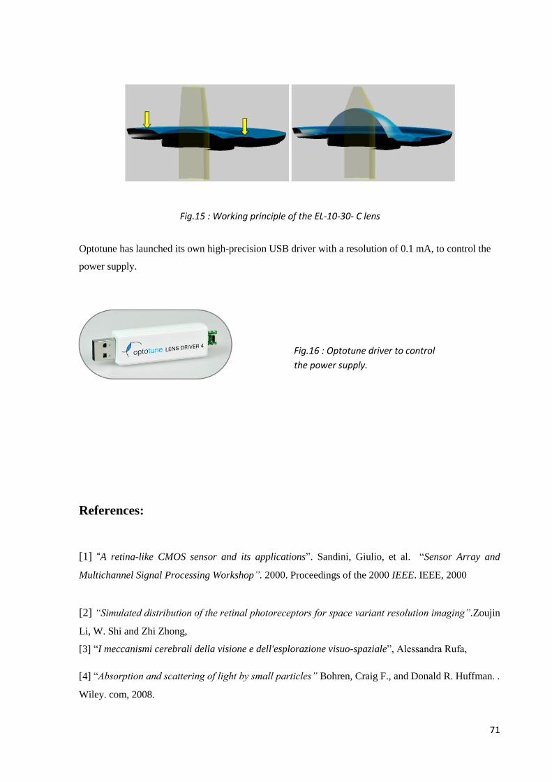
71
Optotune has launched its own high-precision USB driver with a resolution of 0.1 mA, to control the
power supply.
References:
[1] “A retina-like CMOS sensor and its applications”. Sandini, Giulio, et al. “Sensor Array and
Multichannel Signal Processing Workshop”. 2000. Proceedings of the 2000 IEEE. IEEE, 2000
[2] “Simulated distribution of the retinal photoreceptors for space variant resolution imaging”.Zoujin
Li, W. Shi and Zhi Zhong,
[3] “I meccanismi cerebrali della visione e dell'esplorazione visuo-spaziale”, Alessandra Rufa,
[4] “Absorption and scattering of light by small particles” Bohren, Craig F., and Donald R. Huffman. .
Wiley. com, 2008.
Fig.15 : Working principle of the EL-10-30- C lens
Fig.16 : Optotune driver to control
the power supply.

72
[5] “Sensors and Actuators” , Pelrine RE, Kornbluh RD, Joseph JP (1998): cap VII, Electrostriction
of polymer dielectrics with compliant electrodes as a means of actuation. A 64: 77-85
[7] “Mechatronic Muscle: Materials and Technologies”, A. O’Halloran, F. O’Malley, Department of
Electronic Engineering, National University of Ireland Galway],
[7] [8] www.optotune.com
73
Chapter 5
SIMULATION: CST STUDIO SUITE® AND COMSOL
MULTIPHYSICS®
In this chapter I will explain the step followed to make the filter simulation through a 3D model in
CST STUDIO SUITE® and a 2D model in Comsol Multiphysics
®.
5.1 CST STUDIO SUITE ®
CST Studio Suite is an electromagnetic simulation software for arbitrary 3dimensional structures. It
comprises tools for the design and optimization of devices operating in a wide range of frequencies -
static to optical. Analyses may include thermal and mechanical effects, as well as circuit simulation
and electromagnetic simulation.
The software comprises different modules dedicated to specific application areas. For the purpose of
this work, I just studied and used CST MICROWAVE STUDIO® .It enables analysis of antennas,
filters, couplers, planar and multi-layer structures and EMC effects at high frequency.
Before describing the steps followed during the use of CST STUDIO, we explain in short the
simulation method and thus how CST STUDIO SUITE works.
CST STUDIO SUITE is a general-purpose electromagnetic simulator based on the Finite Integration
Technique (FIT). This numerical method provides a universal spatial discretization scheme applicable
to various electromagnetic problems ranging from static field calculations to high frequency
applications in time or frequency domain. Unlike most numerical methods, FIT discretizes the
following integral form of Maxwell’s equations rather than the differential one.
To solve these equations numerically, we must define a finite calculation domain, enclosing the
considered application problem. Creating a suitable mesh system splits this domain up into many
small elements, or grid cells. Discretization of the space into pieces is called mesh. In this way ,
Maxwell’s equations are formulated and solved for each of the cell facets separately . For this reason,
before start simulation, we have to select a properly type of mesh and the frequency of work decides

74
the dimensions of this mesh. As wavelength is smaller and higher will be the amount of mesh and so
their dimensions.
5.1.1 Develop a simulation with CST STUDIO SUITE®
Design a model
The shape creation is one of the most flexible operations. Many different options exist to create the
desired models, as material (selected from a list or built by the user), component (each shape must
have a unique name within a certain component), basic shape creation (the easiest way to create a
shape is to define a “primitive”, like sphere or brick..).
In CST MICROWAVE STUDIO, several different material properties are considered to allow realistic
modeling of practical simulation problems. The two basic materials available are PEC (Perfect
Electrically Conducting material) and Vacuum. Other more complex materials may be defined in the
Material Parameters dialog. For each material is necessary to define some electric and mechanical
properties, as permittivity, dielectric constant, density, etc.
In our case I developed a 3D geometry. I designed a cube sample of Sylgard®184 in which I included
nano-particles of PS with different volumetric densities. These different volumetric density had been
calculated starting from the different concentration of PS suspension which we realized the filters.
Knowing the amount in weight of PS and of Sylgard®184, it was possible to find the quantity of nano-
particles in whole volume. Assuming a sample with cube of Sylgard®184 of 10
4 μm
3(from a cube of
10μm in side ) in side, I found the amount of PS nano-particles in this volume in order to create a
smaller representation corresponding to the real filter. I created two different samples for each filter,
placing the PS nano-particles with a regular arrangement and with a random one. Theoretically our
filter is assumed to be at constant volumetric density, but actually we can’t say for certain that it has
such property. This because we mixed the Sylgard®184 and the nano-particles by hand.
I made also simulations with a geometric model with double thickness and double width in order to
evaluate if different results occurred. The main reason I did this choice is the small dimension of the
model compared to the real filter which has a bigger thickness (about 60 times).
In addition I developed a simulation also for the ideal filter made of nano-particles arranged on an
elettroactive membrane without a matrix as Sylgard®184. The model built with CST STUDIO SUITE
®
is composed of a thin layer of dielectric elastomer with nanopaticles of polystyrene. The two different
states, activated and in rest, was represented by two surface density. Upon electrical activation the
nano-particle density increases as consequence of the membrane deformation towards the centre. Once
the voltage is taken away, the electroactive membrane stretches in the opposite direction with a
decrease in surface density of nano-particles.
Once the geometry is set, we can select the power source characteristics.

75
Exitation source
CST MICROWAVE STUDIO offers several different excitation sources, depending on the specific
application and structure types.
Ports:
Discrete port (They are available as S-Parameter, voltage or current port and are mainly
used to simulate lumped element sources inside the calculation domain).
Waveguide ports (They are used to simulate an infinitely long waveguide, e.g. a
rectangular waveguide, a coaxial cable or a microstrip line).
Field sources:
Plane waves (Excitation of linear, circular or elliptical plane waves).
Far field sources(Import of a farfield monitor file calculated with CST MICROWAVE
STUDIO).
Near field sources(Import of near field source data calculated by CST MICROWAVE
STUDIO, CST CABLE STUDIO, or CST PCB STUDIO).
For my project I selected Plane waves, because I was interested in simulating an incident wave from a
source, located a large distance from the observed object.
When exciting with a plane wave, several conditions must be satisfied, as polarization (can be defined
three types of polarization: linear, circular or elliptical). For linear polarization, one electric field
vector exists for the excitation plane with a fixed direction. This electric field vector changes its
magnitude according to the used excitation signal.
In my work I selected a plane wave as source, because the incident light on the filter (coming from sun
or other light sources) can be assumed enough far from the object to be wave-fronts normal to
the phase velocity vector.
Boundary conditions
Boundary conditions are necessary to solve the Maxwell Equations during the simulation. With this
option we can select how the space around the model will be considered during Maxwell’s Equations
resolution.
As the software works with differential equations we have to impose a condition that the solution has
to take at the extremes (boundary) of the domain.
With boundary conditions a rectangular box is built around the model. The simulation of the structure
will be performed within this boundary box. This box has six faces or planes and it need to define the

76
boundary conditions of each of these planes. The range of frequency of the simulation influences the
volume of this boundary box. And the boundary conditions influence a number of mesh cells which
again influences the accuracy and the time of simulation.
For this project we chose “add-open space” to each side to have a more accurate resolution of
Maxwell’s Equations and to have a bigger plane to display simulation results.
Mesh generation
After we have set up our model geometrically and assigned the appropriate power sources and
boundary conditions, our model has to be translated into a computer accessible format. As already
mentioned above, the FIT method, which is the foundation of CST STUDIO SUITE, is a volume
discretization method. Our calculation domain has to be subdivided into small cells on which
Maxwell’s Grid Equations must be solved. Two different mesh types are available: hexahedral and
tetrahedral. Almost all CST solvers work with a hexahedral mesh, while only some solvers provide a
tetrahedral mesh method.( hexahedral meshing is very robust even for most complex imported
geometries and is highly structured to lead to very fast computations).
The mesh can be selected by a dialog box, where is also possible to chose the Lines per wavelength
(which defines the minimum number of mesh lines in each coordinate direction based on the highest
frequency of evaluation. It describes the spatial sampling rate of the field) ,the Lower mesh limit (this
setting defines the maximum mesh step to be used for the mesh creation) and the Ratio limit (Defines
ratio between the biggest and smallest distance between mesh lines).
From these parameters it appears clear that the wavelength of the electric field source establishes the
number of meshes. In our case, we would like to simulate the scattered field in visible light, that
means frequencies of THz and thus wavelength of hundred nm. It becomes clear that smaller is the
wavelength and bigger is the number of meshes. This entails a large memory requirement to store
results and a very long time of simulation. This is the main limit of the software and it’s the reason
why we couldn’t study the scattered field in visible range, but we restricted the study to infrared
frequencies.

77
In my work I selected just 8 lines per wavelength to reduce the size of my files and to have the
possibility to increase the frequency. Such value is the maximum limit before having wrong result
form simulation.
Start simulation
Just click on “start simulation” and wait for the software to elaborate electric field.
Post processing
The Post Processing enables the visualization of all calculated and monitored results as well as the
computation of several secondary results, for instance S-Parameter, Farfields, SAR values or AR-
Filter.
For the aim of this simulation 2D/3D plot is the most important because it contains interactive
visualization for the most relevant result types. The interactive visualization comprises a
Cutplane Widget (interactive control element allows you to move and rotate the plane
which is used either to clip your 3D plot or to define the plane for the 2D cross section
plot through your 3D field.)
Color Ramp (here we can switch the scaling to logarithmic or dB when pointing the mouse
on the title bar which displays the unit)
2D scalar plots display allows see different type of plot frame and change the visualization.
For example is possible to activate the time animation of the selected scalar plot, or (for
frequency monitors) plot the amplitude of the field vector / component in each point, or also
plot the field vector length / component averaged over all phases. For complex vector fields
Fig. 1: Dialog box to set the mesh
properties in CST STUDIO SUITE®
78
plot, the phase of the selected component can be shown. And of course, start and stop the
animation.
2D vector plot can be used to display 2-dimensional fields as arrows and 3D vector plots to
display three-dimensional fields as arrows or hedgehog.
In this project I saved pictures and exported videos of electric field applied on filter and scattered by
that. The incident electric field is has amplitude of 1 V/m in x and the propagation is in positive z
direction.
Some results are shown in next chapter.
5.2 Comsol Multiphysics ®
COMSOL Multiphysics is a powerful interactive environment for modeling and solving all kinds of
scientific and engineering problems. With COMSOL Multiphysics you can easily extend conventional
models for one type of physics into multiphysics models that solve coupled physics phenomena—and
do so simultaneously.
Using built-in physics user interfaces , we can perform various types of studies including stationary
and time-dependent (transient) studies, Linear and nonlinear studies, Eigenfrequency, modal, and
frequency response studies.
When solving the models, COMSOL Multiphysics uses the proven finite element method (FEM). The
software runs the finite element analysis together with adaptive meshing (if selected) and error control
using a variety of numerical solvers. We can use COMSOL Multiphysics in many application areas as
Acoustics, Fluid dynamics, Electromagnetics, Heat transfer etc.
Radio-Frequency Module
Most of the problems that are solved with COMSOL Multiphysics are three-dimensional (3D) in the
real world. In many cases, it is sufficient to solve a two-dimensional (2D) problem that is close to or
equivalent to the real problem. Furthermore, it is good practice to start a modeling project by building
one or several 2D models before going to a 3D model. This is because 2D models are easier to modify
and solve much faster.
For these reasons I developed a 2D model for each filter, in order to complete different results and
obtain have a more accurate simulation of my device.
An important technique to minimize the problem size is to use efficient boundary conditions.
Truncating the geometry without introducing too large errors is one of the great challenges in

79
modeling. To do this Comsol Multiphysics® offers a technique based on Perfected Matched Layer
(PML). PMLs are layers that absorbs all radiated waves with small reflections. For this reason I made
a finite model surrounded by PML without a huge requirement of memory during simulation and at
the same time with minimum errors.
5.2.1 Develop a simulation with Comsol Multiphysics®
As CST STUDIO SUITE® the simulation starts from a geometry designing followed by a sequence of
other definitions, such electric source and boundary conditions. Below we explain only the main step I
followed during the model building.
Design a geometry
Also in this software, the geometry is one of the most important thing to do accurately. It will
represent our model and will be the start point of the simulation.
A 2D geometry was chosen for this study: a square surface of side 10μm , where I inserted circles of
radius 205μm. The square represents the matrix made of Sylgard184® and the circles represent the
nano-particles of polystyrene. Also in this software project, I developed to different density to show
the scattering by a random and a regular pattern of particles inside the silicon matrix.
Materials
Each geometry component must has its material specified. So I selected the right materials and set the
appropriate characteristics.
Simulation
The frequency domain was already set at the beginning, so we had to chose the frequency range and
define the electric field source.
In my case I made simulations with two different frequencies: 300 THz and 400 THz. The aim was to
study the model in the whole visible range, but such values required too much memory space. So I had
to limit the simulation at these two frequencies even if they don’t belong to the desired range. Note
that 400THz is very near the red color frequency, so it can be considered a significant value for my
simulation.
Results visualization

80
Results are shown in a 2D plot, where the incident and scattered electric fields are displayed together.
The incident electric field is has amplitude of 1 V/m in z and the propagation is in negative x direction.
The plots displayed in the graphic window in Comsol Multiphysics®
are in next chapter.
81
Chapter 6
PROTOTYPING: METHODS AND MATERIALS
Considering the general architecture of the system developed, described in detail in chapter 4, below
are specified the materials used and the main methods used to realize the various components:
Filter
To make realize the filter we used nano-particles of polystyrene and an electroactive
membrane as support.
Frames
The frames has been designed in Solidworks and realized in ABS with a 3D printer at “Centro
Piaggio Researcher Centre”
The housing
It has been designed in Solidworks environment and realized in ABS with a 3D printer at
“Centro Piaggio Researcher Centre.
6.1 Filter
The filter was created from a dielectrict elastomer tape and pre-stretched in order to have an increase
of 400% in area and a reduction of thickness from 1mm to 62.5 μm. Thus it was attached to a circular
frame and utilized as a base for particles.
The polymer used is a VHB™ Adhesive Transfer Tape. It is an acrylate pressure sensitive adhesive
(PSA). The chemical bonds that make up the polymer chains consist of carbon-carbon single bonds
that are highly resistant to energy in the form of heat or ultraviolet light, as well as chemical attack.
The VHB™ Adhesive Transfer Tape F-9473PC yielded 92% retention of peel adhesion after the roll
was aged for more than 5 years at 150°F (65°C). Bonds made with VHB™ Tapes can tolerate
periodic, short-term exposures to temperatures up to 500°F (260°C).
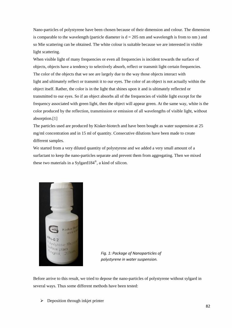
82
Nano-particles of polystyrene have been chosen because of their dimension and colour. The dimension
is comparable to the wavelength (particle diameter is d = 205 nm and wavelength is from to nm ) and
so Mie scattering can be obtained. The white colour is suitable because we are interested in visible
light scattering.
When visible light of many frequencies or even all frequencies is incident towards the surface of
objects, objects have a tendency to selectively absorb, reflect or transmit light certain frequencies.
The color of the objects that we see are largely due to the way those objects interact with
light and ultimately reflect or transmit it to our eyes. The color of an object is not actually within the
object itself. Rather, the color is in the light that shines upon it and is ultimately reflected or
transmitted to our eyes. So if an object absorbs all of the frequencies of visible light except for the
frequency associated with green light, then the object will appear green. At the same way, white is the
color produced by the reflection, transmission or emission of all wavelengths of visible light, without
absorption.[1]
The particles used are produced by Kisker-biotech and have been bought as water suspension at 25
mg/ml concentration and in 15 ml of quantity. Consecutive dilutions have been made to create
different samples.
We started from a very diluted quantity of polystyrene and we added a very small amount of a
surfactant to keep the nano-particles separate and prevent them from aggregating. Then we mixed
these two materials in a Sylgard184®, a kind of silicon.
Before arrive to this result, we tried to depose the nano-particles of polystyrene without sylgard in
several ways. Thus some different methods have been tested:
Deposition through inkjet printer
Fig. 1: Package of Nanoparticles of
polystyrene in water suspension.
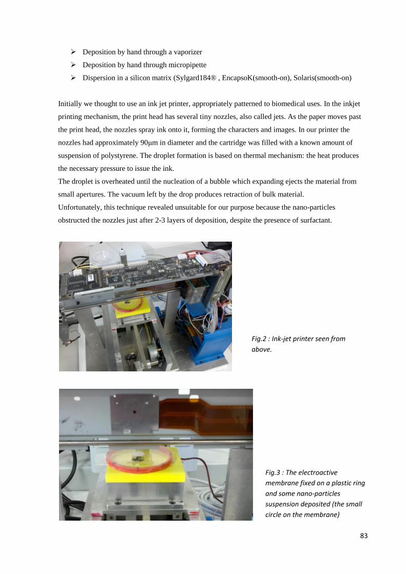
83
Deposition by hand through a vaporizer
Deposition by hand through micropipette
Dispersion in a silicon matrix (Sylgard184® , EncapsoK(smooth-on), Solaris(smooth-on)
Initially we thought to use an ink jet printer, appropriately patterned to biomedical uses. In the inkjet
printing mechanism, the print head has several tiny nozzles, also called jets. As the paper moves past
the print head, the nozzles spray ink onto it, forming the characters and images. In our printer the
nozzles had approximately 90μm in diameter and the cartridge was filled with a known amount of
suspension of polystyrene. The droplet formation is based on thermal mechanism: the heat produces
the necessary pressure to issue the ink.
The droplet is overheated until the nucleation of a bubble which expanding ejects the material from
small apertures. The vacuum left by the drop produces retraction of bulk material.
Unfortunately, this technique revealed unsuitable for our purpose because the nano-particles
obstructed the nozzles just after 2-3 layers of deposition, despite the presence of surfactant.
Fig.2 : Ink-jet printer seen from
above.
Fig.3 : The electroactive
membrane fixed on a plastic ring
and some nano-particles
suspension deposited (the small
circle on the membrane)
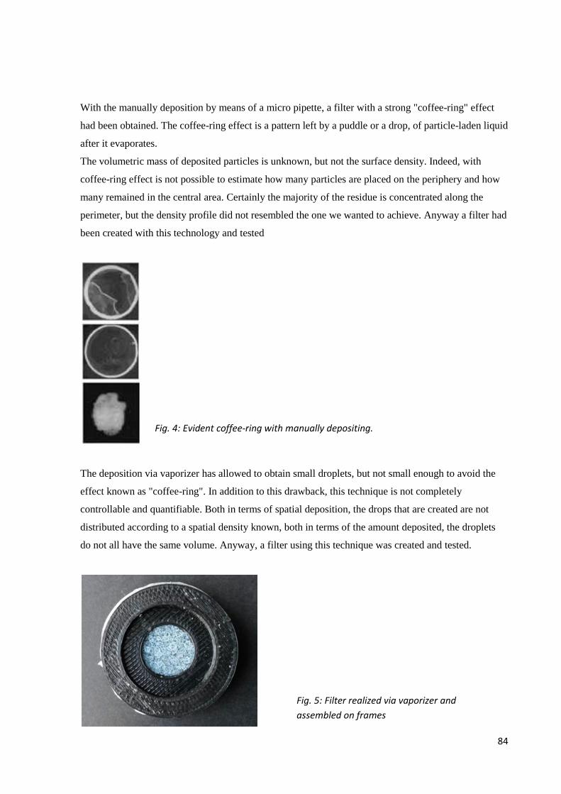
84
With the manually deposition by means of a micro pipette, a filter with a strong "coffee-ring" effect
had been obtained. The coffee-ring effect is a pattern left by a puddle or a drop, of particle-laden liquid
after it evaporates.
The volumetric mass of deposited particles is unknown, but not the surface density. Indeed, with
coffee-ring effect is not possible to estimate how many particles are placed on the periphery and how
many remained in the central area. Certainly the majority of the residue is concentrated along the
perimeter, but the density profile did not resembled the one we wanted to achieve. Anyway a filter had
been created with this technology and tested
The deposition via vaporizer has allowed to obtain small droplets, but not small enough to avoid the
effect known as "coffee-ring". In addition to this drawback, this technique is not completely
controllable and quantifiable. Both in terms of spatial deposition, the drops that are created are not
distributed according to a spatial density known, both in terms of the amount deposited, the droplets
do not all have the same volume. Anyway, a filter using this technique was created and tested.
Fig. 4: Evident coffee-ring with manually depositing.
Fig. 5: Filter realized via vaporizer and
assembled on frames

85
Finally, we realized different samples composed by PS nano-particles, surfactant (Tween20) and a
silicon, Sylgard®184. This approach showed to be the most promising between all the others.
As before mentioned with the ink-jet printer method, we added some surfactant to avoid the particles
aggregation. At the same time we couldn’t use too much of it because it made sylgard184 opaque. So
we found the right quantity of surfactant to use and it was of about 2μl per 2g of Sylgard®184 .
Therefore the materials used are:
Nano-particles of PS in suspension of 1mg/ml and 5mg/ml, Tween20 (surfactant) and Sylgard®184
(monomer and curing agent mixed in a ratio of 20 parts monomer to one part curing agent).
The method followed in the realization of the filters can be schematized as:
- Pouring three different quantities of PS suspension (200μl, 500 μl and 1ml) at the first
concentration in three Petri dishes.
- Let a 2μl droplet of Tween20 to fall on the three amounts of PS in order to “break” them
because of surface tension decrease.
- Let the water (of the PS suspension) evaporate.
- Add monomer (2g).
- Add curing agent (100μl so in 1:20 ratio).
- Mix well.
- Collocate in vacuum machine to remove air bubbles arisen while mixing.
- Let the sample curing for 24 hours at environmental temperature or 4 hours in oven at 65°.
Repeat the whole method for the second concentration of PS suspension (5mg/ml). Also a sample
with only Sylgard®184 had been created.
After the filters realization phases, we passed to the measuring of blurring effect generated by the
filters.
The resolution measurements were obtained through images processing. We took some photos with a
EOS 60D camera, EFS 18-35 mm lens, the sample to test and a target as the object of the image.
The system setup can be explained as follows:
- Camera lens assembled with the camera and set at a 135mm focal length and activated the
auto-focus.
- Placement of the sample at 6cm from the end of the camera in order to be in a good point of
FoV (Fiel of View of the camera).
- Target location at 20cm from the sample.
- Taking photo trying not to move the camera (a remote control would be a good solution to
avoid blurring due to the hand shutter click).
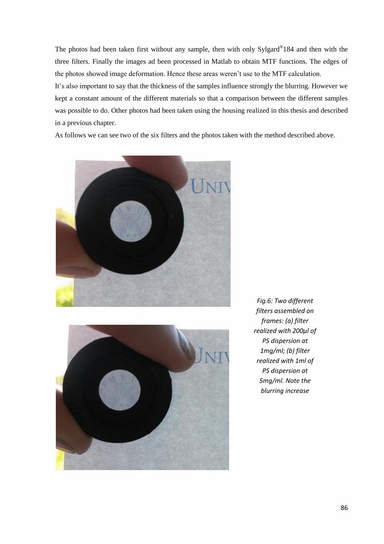
86
The photos had been taken first without any sample, then with only Sylgard®184 and then with the
three filters. Finally the images ad been processed in Matlab to obtain MTF functions. The edges of
the photos showed image deformation. Hence these areas weren’t use to the MTF calculation.
It’s also important to say that the thickness of the samples influence strongly the blurring. However we
kept a constant amount of the different materials so that a comparison between the different samples
was possible to do. Other photos had been taken using the housing realized in this thesis and described
in a previous chapter.
As follows we can see two of the six filters and the photos taken with the method described above.
Fig.6: Two different
filters assembled on
frames: (a) filter
realized with 200μl of
PS dispersion at
1mg/ml; (b) filter
realized with 1ml of
PS dispersion at
5mg/ml. Note the
blurring increase
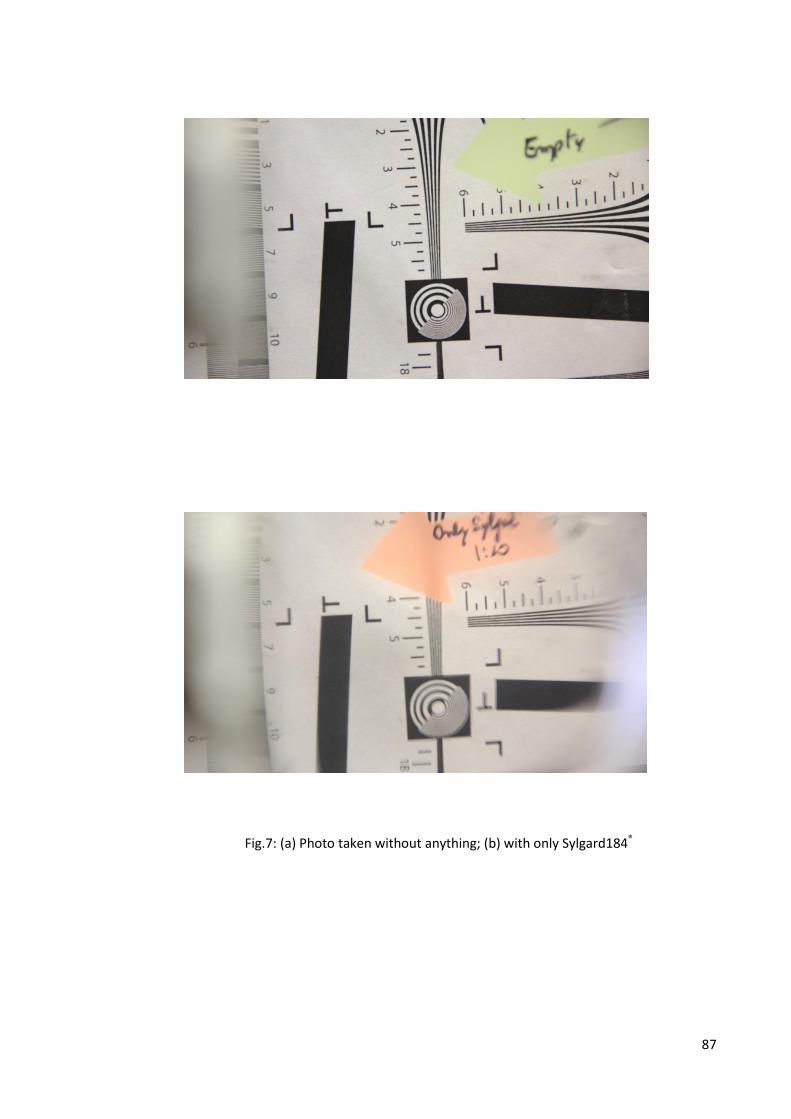
87
Fig.7: (a) Photo taken without anything; (b) with only Sylgard184®
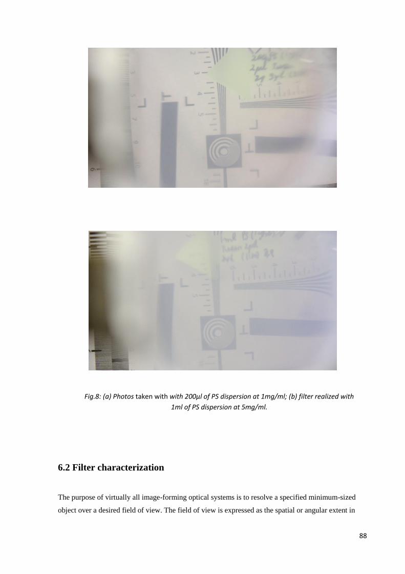
88
6.2 Filter characterization
The purpose of virtually all image-forming optical systems is to resolve a specified minimum-sized
object over a desired field of view. The field of view is expressed as the spatial or angular extent in
Fig.8: (a) Photos taken with with 200μl of PS dispersion at 1mg/ml; (b) filter realized with
1ml of PS dispersion at 5mg/ml.
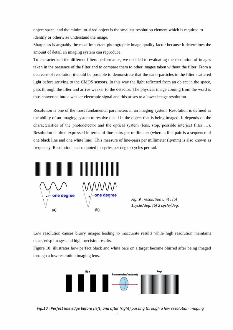
89
object space, and the minimum-sized object is the smallest resolution element which is required to
identify or otherwise understand the image.
Sharpness is arguably the most important photographic image quality factor because it determines the
amount of detail an imaging system can reproduce.
To characterized the different filters performance, we decided to evaluating the resolution of images
taken in the presence of the filter and to compare them to other images taken without the filter. From a
decrease of resolution it could be possible to demonstrate that the nano-particles in the filter scattered
light before arriving to the CMOS sensors. In this way the light reflected from an object in the space,
pass through the filter and arrive weaker to the detector. The physical image coming from the word is
thus converted into a weaker electronic signal and this arises to a lower image resolution.
Resolution is one of the most fundamental parameters in an imaging system. Resolution is defined as
the ability of an imaging system to resolve detail in the object that is being imaged. It depends on the
characteristics of the photodetector and the optical system (lens, stop, possible interject filter …).
Resolution is often expressed in terms of line-pairs per millimeter (where a line-pair is a sequence of
one black line and one white line). This measure of line-pairs per millimeter (lp/mm) is also known as
frequency. Resolution is also quoted in cycles per deg or cycles per rad.
Low resolution causes blurry images leading to inaccurate results while high resolution maintains
clear, crisp images and high precision results.
Figure 10 illustrates how perfect black and white bars on a target become blurred after being imaged
through a low resolution imaging lens.
Fig. 9 : resolution unit : (a)
1cycle/deg, (b) 2 cycle/deg.
Fig.10 : Perfect line edge before (left) and after (right) passing through a low resolution imaging
lens.
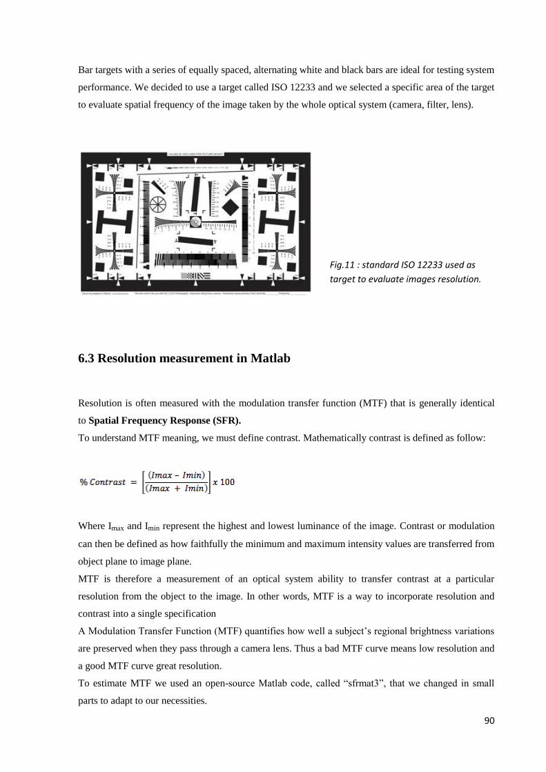
90
Bar targets with a series of equally spaced, alternating white and black bars are ideal for testing system
performance. We decided to use a target called ISO 12233 and we selected a specific area of the target
to evaluate spatial frequency of the image taken by the whole optical system (camera, filter, lens).
6.3 Resolution measurement in Matlab
Resolution is often measured with the modulation transfer function (MTF) that is generally identical
to Spatial Frequency Response (SFR).
To understand MTF meaning, we must define contrast. Mathematically contrast is defined as follow:
Where Imax and Imin represent the highest and lowest luminance of the image. Contrast or modulation
can then be defined as how faithfully the minimum and maximum intensity values are transferred from
object plane to image plane.
MTF is therefore a measurement of an optical system ability to transfer contrast at a particular
resolution from the object to the image. In other words, MTF is a way to incorporate resolution and
contrast into a single specification
A Modulation Transfer Function (MTF) quantifies how well a subject’s regional brightness variations
are preserved when they pass through a camera lens. Thus a bad MTF curve means low resolution and
a good MTF curve great resolution.
To estimate MTF we used an open-source Matlab code, called “sfrmat3”, that we changed in small
parts to adapt to our necessities.
Fig.11 : standard ISO 12233 used as
target to evaluate images resolution.
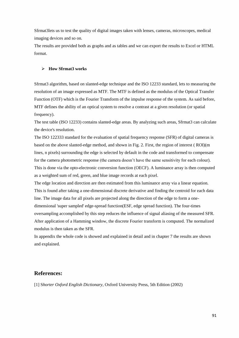
91
Sfrmat3lets us to test the quality of digital images taken with lenses, cameras, microscopes, medical
imaging devices and so on.
The results are provided both as graphs and as tables and we can export the results to Excel or HTML
format.
How Sfrmat3 works
Sfrmat3 algorithm, based on slanted-edge technique and the ISO 12233 standard, lets to measuring the
resolution of an image expressed as MTF. The MTF is defined as the modulus of the Optical Transfer
Function (OTF) which is the Fourier Transform of the impulse response of the system. As said before,
MTF defines the ability of an optical system to resolve a contrast at a given resolution (or spatial
frequency).
The test table (ISO 12233) contains slanted-edge areas. By analyzing such areas, Sfrmat3 can calculate
the device's resolution.
The ISO 122333 standard for the evaluation of spatial frequency response (SFR) of digital cameras is
based on the above slanted-edge method, and shown in Fig. 2. First, the region of interest ( ROI)(m
lines, n pixels) surrounding the edge is selected by default in the code and transformed to compensate
for the camera photometric response (the camera doesn’t have the same sensitivity for each colour).
This is done via the opto-electronic conversion function (OECF). A luminance array is then computed
as a weighted sum of red, green, and blue image records at each pixel.
The edge location and direction are then estimated from this luminance array via a linear equation.
This is found after taking a one-dimensional discrete derivative and finding the centroid for each data
line. The image data for all pixels are projected along the direction of the edge to form a one-
dimensional 'super sampled' edge-spread function(ESF, edge spread function). The four-times
oversampling accomplished by this step reduces the influence of signal aliasing of the measured SFR.
After application of a Hamming window, the discrete Fourier transform is computed. The normalized
modulus is then taken as the SFR.
In appendix the whole code is showed and explained in detail and in chapter 7 the results are shown
and explained.
References:
[1] Shorter Oxford English Dictionary, Oxford University Press, 5th Edition (2002)
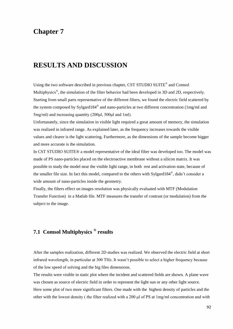
92
Chapter 7
RESULTS AND DISCUSSION
Using the two software described in previous chapter, CST STUDIO SUITE® and Comsol
Multiphysics®, the simulation of the filter behavior had been developed in 3D and 2D, respectively.
Starting from small parts representative of the different filters, we found the electric field scattered by
the system composed by Sylgard184® and nano-particles at two different concentration (1mg/ml and
5mg/ml) and increasing quantity (200μl, 500μl and 1ml).
Unfortunately, since the simulation in visible light required a great amount of memory, the simulation
was realized in infrared range. As explained later, as the frequency increases towards the visible
values and clearer is the light scattering. Furthermore, as the dimensions of the sample become bigger
and more accurate is the simulation.
In CST STUDIO SUITE® a model representative of the ideal filter was developed too. The model was
made of PS nano-particles placed on the electroactive membrane without a silicon matrix. It was
possible to study the model near the visible light range, in both rest and activation state, because of
the smaller file size. In fact this model, compared to the others with Sylgard184®, didn’t consider a
wide amount of nano-particles inside the geometry.
Finally, the filters effect on images resolution was physically evaluated with MTF (Modulation
Transfer Function) in a Matlab file. MTF measures the transfer of contrast (or modulation) from the
subject to the image.
7.1 Comsol Multiphysics ® results
After the samples realization, different 2D studies was realized. We observed the electric field at short
infrared wavelength, in particular at 300 THz. It wasn’t possible to select a higher frequency because
of the low speed of solving and the big files dimensions.
The results were visible in static plot where the incident and scattered fields are shown. A plane wave
was chosen as source of electric field in order to represent the light sun or any other light source.
Here some plot of two more significant filters. One made with the highest density of particles and the
other with the lowest density ( the filter realized with a 200 μl of PS at 1mg/ml concentration and with
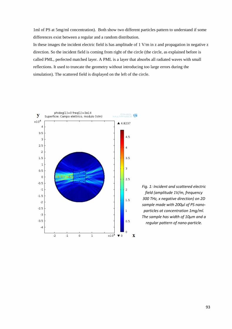
93
1ml of PS at 5mg/ml concentration). Both show two different particles pattern to understand if some
differences exist between a regular and a random distribution.
In these images the incident electric field is has amplitude of 1 V/m in z and propagation in negative z
direction. So the incident field is coming from right of the circle (the circle, as explained before is
called PML, perfected matched layer. A PML is a layer that absorbs all radiated waves with small
reflections. It used to truncate the geometry without introducing too large errors during the
simulation). The scattered field is displayed on the left of the circle.
Fig. 1: Incident and scattered electric
field (amplitude 1V/m, frequency
300 THz, x negative direction) on 2D
sample made with 200μl of PS nano-
particles at concentration 1mg/ml.
The sample has width of 10μm and a
regular pattern of nano-particle.
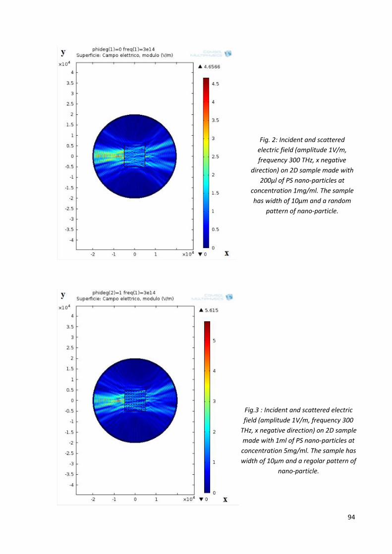
94
Fig. 2: Incident and scattered
electric field (amplitude 1V/m,
frequency 300 THz, x negative
direction) on 2D sample made with
200μl of PS nano-particles at
concentration 1mg/ml. The sample
has width of 10μm and a random
pattern of nano-particle.
Fig.3 : Incident and scattered electric
field (amplitude 1V/m, frequency 300
THz, x negative direction) on 2D sample
made with 1ml of PS nano-particles at
concentration 5mg/ml. The sample has
width of 10μm and a regolar pattern of
nano-particle.
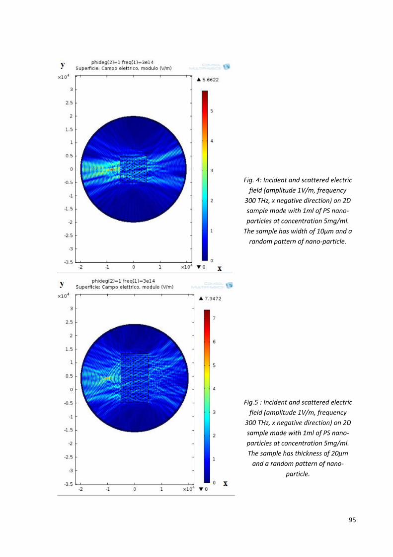
95
Fig. 4: Incident and scattered electric
field (amplitude 1V/m, frequency
300 THz, x negative direction) on 2D
sample made with 1ml of PS nano-
particles at concentration 5mg/ml.
The sample has width of 10μm and a
random pattern of nano-particle.
Fig.5 : Incident and scattered electric
field (amplitude 1V/m, frequency
300 THz, x negative direction) on 2D
sample made with 1ml of PS nano-
particles at concentration 5mg/ml.
The sample has thickness of 20μm
and a random pattern of nano-
particle.
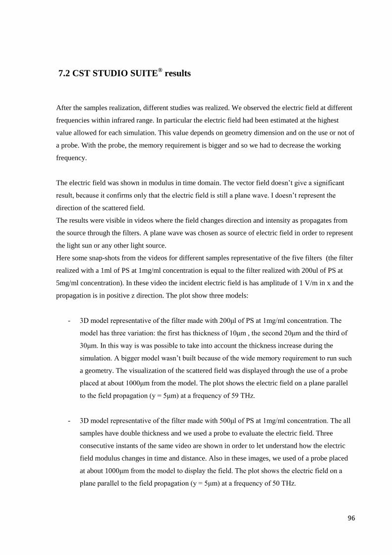
96
7.2 CST STUDIO SUITE® results
After the samples realization, different studies was realized. We observed the electric field at different
frequencies within infrared range. In particular the electric field had been estimated at the highest
value allowed for each simulation. This value depends on geometry dimension and on the use or not of
a probe. With the probe, the memory requirement is bigger and so we had to decrease the working
frequency.
The electric field was shown in modulus in time domain. The vector field doesn’t give a significant
result, because it confirms only that the electric field is still a plane wave. I doesn’t represent the
direction of the scattered field.
The results were visible in videos where the field changes direction and intensity as propagates from
the source through the filters. A plane wave was chosen as source of electric field in order to represent
the light sun or any other light source.
Here some snap-shots from the videos for different samples representative of the five filters (the filter
realized with a 1ml of PS at 1mg/ml concentration is equal to the filter realized with 200ul of PS at
5mg/ml concentration). In these video the incident electric field is has amplitude of 1 V/m in x and the
propagation is in positive z direction. The plot show three models:
- 3D model representative of the filter made with 200μl of PS at 1mg/ml concentration. The
model has three variation: the first has thickness of 10μm , the second 20μm and the third of
30μm. In this way is was possible to take into account the thickness increase during the
simulation. A bigger model wasn’t built because of the wide memory requirement to run such
a geometry. The visualization of the scattered field was displayed through the use of a probe
placed at about 1000μm from the model. The plot shows the electric field on a plane parallel
to the field propagation (y = 5μm) at a frequency of 59 THz.
- 3D model representative of the filter made with 500μl of PS at 1mg/ml concentration. The all
samples have double thickness and we used a probe to evaluate the electric field. Three
consecutive instants of the same video are shown in order to let understand how the electric
field modulus changes in time and distance. Also in these images, we used of a probe placed
at about 1000μm from the model to display the field. The plot shows the electric field on a
plane parallel to the field propagation (y = 5μm) at a frequency of 50 THz.
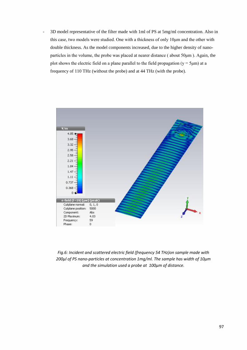
97
- 3D model representative of the filter made with 1ml of PS at 5mg/ml concentration. Also in
this case, two models were studied. One with a thickness of only 10μm and the other with
double thickness. As the model components increased, due to the higher density of nano-
particles in the volume, the probe was placed at nearer distance ( about 50μm ). Again, the
plot shows the electric field on a plane parallel to the field propagation (y = 5μm) at a
frequency of 110 THz (without the probe) and at 44 THz (with the probe).
Fig.6: Incident and scattered electric field (frequency 54 THz)on sample made with
200μl of PS nano-particles at concentration 1mg/ml. The sample has width of 10μm
and the simulation used a probe at 100μm of distance.
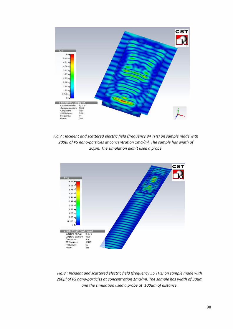
98
Fig.7 : Incident and scattered electric field (frequency 94 THz) on sample made with
200μl of PS nano-particles at concentration 1mg/ml. The sample has width of
20μm. The simulation didn’t used a probe.
Fig.8 : Incident and scattered electric field (frequency 55 THz) on sample made with
200μl of PS nano-particles at concentration 1mg/ml. The sample has width of 30μm
and the simulation used a probe at 100μm of distance.
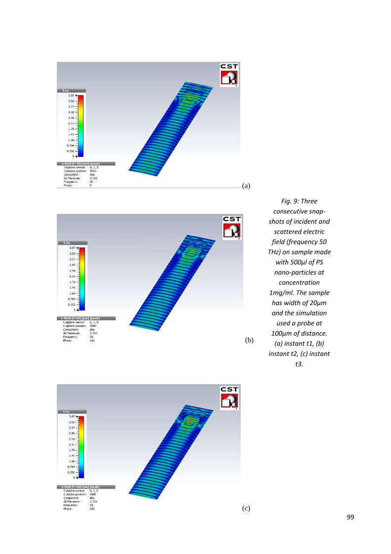
99
(a)
(b)
(c)
Fig. 9: Three
consecutive snap-
shots of incident and
scattered electric
field (frequency 50
THz) on sample made
with 500μl of PS
nano-particles at
concentration
1mg/ml. The sample
has width of 20μm
and the simulation
used a probe at
100μm of distance.
(a) instant t1, (b)
instant t2, (c) instant
t3.
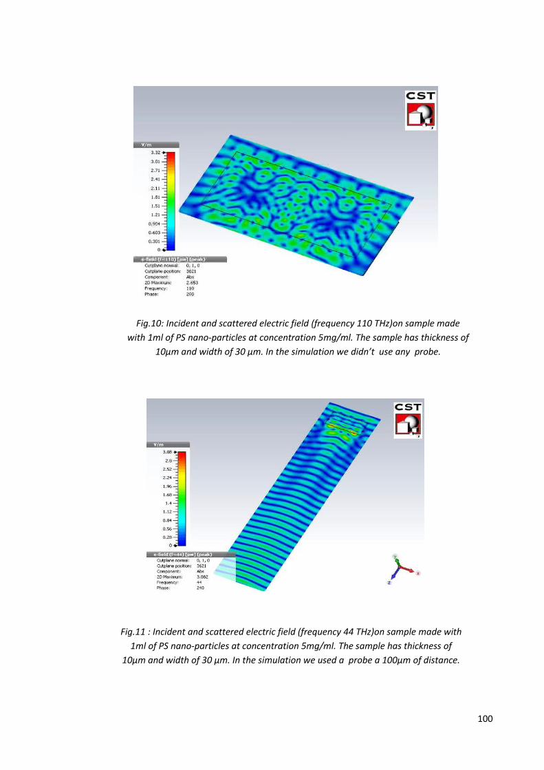
100
Fig.10: Incident and scattered electric field (frequency 110 THz)on sample made
with 1ml of PS nano-particles at concentration 5mg/ml. The sample has thickness of
10μm and width of 30 μm. In the simulation we didn’t use any probe.
Fig.11 : Incident and scattered electric field (frequency 44 THz)on sample made with
1ml of PS nano-particles at concentration 5mg/ml. The sample has thickness of
10μm and width of 30 μm. In the simulation we used a probe a 100μm of distance.

101
( a )
( b )
( c )
Fig.12 : Three
consecutive snap-
shots of incident and
scattered electric
field (frequency 39
THz) on sample made
with 1ml of PS nano-
particles at
concentration
5mg/ml. The sample
has width of 20μm
and the simulation
used a probe at
50μm of distance. (a)
instant t1, (b) instant
t2, (c) instant t3.
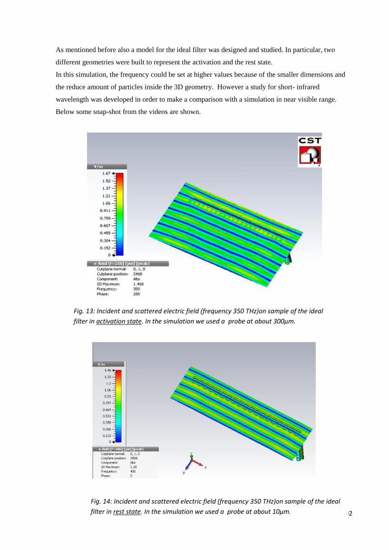
102
As mentioned before also a model for the ideal filter was designed and studied. In particular, two
different geometries were built to represent the activation and the rest state.
In this simulation, the frequency could be set at higher values because of the smaller dimensions and
the reduce amount of particles inside the 3D geometry. However a study for short- infrared
wavelength was developed in order to make a comparison with a simulation in near visible range.
Below some snap-shot from the videos are shown.
Fig. 13: Incident and scattered electric field (frequency 350 THz)on sample of the ideal
filter in activation state. In the simulation we used a probe at about 300μm.
Fig. 14: Incident and scattered electric field (frequency 350 THz)on sample of the ideal
filter in rest state. In the simulation we used a probe at about 10μm.

103
Fig. 16: Incident and scattered electric field (frequency 40 THz)on sample of the
ideal filter in rest state. In the simulation we used a probe at a distance of 20μm.
Fig. 15: Incident and scattered electric field (frequency 40 THz)on sample of the
ideal filter in activation state. In the simulation we used a probe at a distance of
100μm.

104
7.3 Experimental evaluation: resolution measurement in Matlab
As explained in chapter 6, the filters effect on image resolution has been estimated in Matlab with the
Modulation Transfer Function. The code, called “sfrmat3”, was downloaded from internet but
modified to our purpose.
A main code was developed to call “sfrmat3” and calculate MTF for ten images taken with each filter.
The MTF obtained were averaged, saved in a excel file and displayed in a plot. Thus a comparison
between different filters could be made both in numerical and graphical way.
The imaging system was made of :
- Camera ( Imaging Source DMK 23GM021 )
- Filter
- Lens ( Optotune Lens EL-10-30-C )
- Target ( ISO 12233 )
In particular we evaluated MTF in eight cases: without any device between the camera and the target,
with a filter made only of Sylgard184® and with the six filters we realized.
“Sfrmat3” refers and thus displays SFR (Space Frequency Response ) instead of MTF. Here the two
function can be considered equivalent ( the SFR is a measurement of the effective system MTF
relative to the test object feature used ). SRF is estimated for R,G,B channel separately, as the camera
takes color images, versus spatial frequency, in line/mm.
Below we show four significant plots are shown. They represents the MTF in four cases:
- Without any device between the camera and the lens
- Only in the presence of Sylgard184®
- With the filter made of 200μl of PS at concentration 1mg/ml
- With the filter made of 1ml of PS at concentration 5mg/ml
Thus we can see how the resolution changes (decreases) as the volumetric density of PS increases.
Plot can be explained as follows: where SFRis equal to 1, it means that the contrast vs spatial
frequency is maximum. Where SFR is equal to 0.5, it means that MTF falls to 50% of its low
frequency value. The values are affected by some noise thus the three curves (R,G,B) are not similar in
some parts.
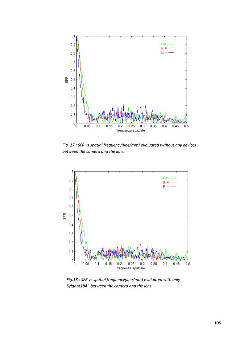
105
Fig. 17 : SFR vs spatial frequency(line/mm) evaluated without any devices
between the camera and the lens.
Fig.18 : SFR vs spatial frequency(line/mm) evaluated with only
Sylgard184® between the camera and the lens.
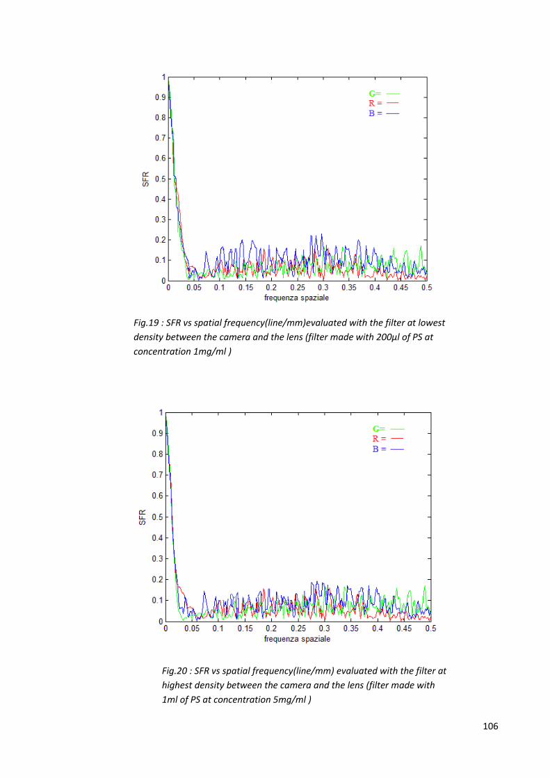
106
Fig.19 : SFR vs spatial frequency(line/mm)evaluated with the filter at lowest
density between the camera and the lens (filter made with 200μl of PS at
concentration 1mg/ml )
Fig.20 : SFR vs spatial frequency(line/mm) evaluated with the filter at
highest density between the camera and the lens (filter made with
1ml of PS at concentration 5mg/ml )
107
7.4 Discussion of results
Analyzing the results obtained in CST STUDIO SUITE®
we make a distinction between the 3D
models containing Sylgard184®
and the ideal filter model.
With regard to the models containing Sylgard184®
, a first consideration must be taken into account
about CST simulations.
The working frequency does not belong to the visible range but infrared range. This is due to the large
computational cost and large memory requirement to mesh the volume of the model (the mesh is
necessary to solve Maxwell’s equations).
As the working frequency rises (and consequentially the wavelength decreases) and finer is the mesh
and in visible light the frequency is 300 THz compared to about 50 THz of large infrared waves. So
there is more than one order in magnitude. For the simulations the highest working frequency admitted
had been chosen .This depends also on the presence or not of a probe . Indeed, the use of these tools
for the evaluation and visualization of the magnetic field required a considerable amount of memory.
The simulations had been thus a compromise between the field visualization at a great distance (thus
with a probe) and a higher working frequency .
From these considerations we can say that despite the characterization software in the visible has not
been reached , the simulation in IR is a good point of departure for future characterizations.
Indeed we must note that as the frequency increases, the scattering behavior becomes more and more
pronounced. This because decreasing the incident field wavelength, the scattering observed tends to
move from Rayleigh scattering to Mie scattering . This one is exactly the physical phenomenon
underlying the behavior of our filter.
The other consideration that is good to keep in mind is that the simulations were carried out on very
small models compared to the real devices . This fact leads to not completely accurate results, but that,
however, are essential to have a first idea about the behavior of the filters. Models with double or
triple thickness were made to demonstrate that the bigger amount of particles in them scatters the field
more significantly .
It’s therefore reasonable to expect that , in the real case, where the thickness of the filter is
approximately mm so one hundred times higher than the models dimension, the effect of scattering is
definitely much stronger.
Also the width of the filter affects the global behavior. In fact, from simulations performed on models
with the same thickness and double width, we can see how the field is deflected in a divergent
direction relative to the filter surface.
Finally, even the particles distribution patter has a slight effect on the scattered field. Particles
positioned randomly in the volume demonstrate to scatter more the field.
108
Basically they create repeated reflections within the sample that generate,in output, waves of electric
field not in phase and in different directions.
All these statements are also confirmed by the decrease in the modulus of the field in the filter output.
This is visible by staining graphics which refers to the scales at the side of the field. Looking at these
scales we can see that they specify decreasing values as the volumetric density of particles increases.
So the greater the presence of particles within the model and more pronounced is the effect that these
have on the field.
These conclusions are also confirmed by simulations in Comsol Multiphysics®
despite these models
are simpler since they are 2D. From the produce plot, we note that the sensible effect of rays focusing
in the first filter (due to high component Sylgard ® which however is used to build lens with variable
curvature) tends to almost disappear in the filter with maximum polystyrene density.
Again in this software, an increase in the presence of particles and in thickness of the model causes a
substantial increase in the phenomenon of scattering.
Similar considerations can be made with the models created to characterize a filter with particles
placed directly on the electroactive membrane. The simulations made in CST STUDIO SUITE®
showed that in the rest state, where the voltage is zero, the particles, which are to bigger distance from
one another, tend to scatter the field less. In the activation state, ie when the applied voltage to the
membrane is approximately 5KV, the particles that had a certain distance with the near ones, are now
located very close one to an other. This implies that they scatter the electric field more efficiently than
the case where the voltage was 0V.
Obviously also in this simulation the dimensions are small compared to the one of a real filter.
Finally also in this model has been demonstrated that as the frequency increases the phenomenon of
scattering becomes more intense.
The experimental evaluation carried out through MTF calculus confirmed that a decrease of resolution
occurs with an increasing particle density.
From the plot we see that the resolution falls faster towards lower values in case of higher PS density
(filter made with 1ml suspension of PS concentration 5mg/ml).
The presence of only Sylgard ® does not significantly change the spatial resolution values . Indeed, its
properties of transparency makes this material suitable to build polymeric tunable lenses in the field
search.
This is noticeably visible from the charts, but it is clear in the results saved in excel file. The values of
the MTF corresponding to the same spatial frequencies are higher in the case of the first filter
compared to the second.
109
Chapter 8
CONCLUSION AND FUTURE WORK
This work was initially aimed at designing an electrically tuneable optical filter based on light
scattering (within the visible spectrum of wavelengths 400 - 700 nm) in order to mimic the foveal
vision in human eyes. Unfortunately the lack of a suitable instrument to place the nano-particles of PS
on an electroactive membrane did not make it possible.
In a future perspective there are certainly parts to be improved. Of course starting from the filter
production which requires a different or better tool to use the nano-particle.
The presence of Sylgard184® was fundamental for this work, but not perfect . Indeed Sylgard184
® has
a certain focusing effect of the rays as it’s used to produce tunable lenses in field research. The
technique of production where we used this material is certainly the most promising, but a different or
a improved method to place particles in the matrix is required.
Moreover, the presence of Sylgard184® reduces the membrane electroactive performance with regard
to the stretching ability. Experiments with small silicone plates placed on the membrane, conducted at
Centro Piaggio Research Centre, showed a reduction of deformation in presence of such material.
From the best results equal to a 20 % of membrane deformation (in case the ratio between the area
dedicated to the electrodes and the inner one with only dielectric equal to 50% ) , they passed to a
deformation of 5 - 10 % . So the presence of Sylgard184® on the membrane greatly reduces the
performance of the dielectric elastomer. This is due to the silicone behaviour to counteract the force
exerted by the membrane during the electric activation. Maybe a material with lower Young's modulus
could solve or reduce this phenomenon.
Another problem is represented by the simulation techniques that are not completely suitable for a
study in the visible range. CST STUDIO SUITE® ,for example, is used mainly to study antennas. In
particular to understand the radiated field in near and far-field. However it has to be highlighted that
perhaps simulations with a higher frequency could have been made provided that a bigger space to
store results was available.
In conclusion we can say that this first realization of a filter based on light scattering, reduced the
resolution of an optical system. The thickness and the presence of a bigger amount of particles effect
however the filter behaviour. In future it will be necessary to understand what is the best value of
thickness to have a significant change in scattering without invalidate the electroactive membrane
performance. Also search another tool to use the particles without Sylgard184®
should be a challenge
to make a real tuneable optical filter.

110
APPENDIX
“SFRMAT” per il calcolo della MTF
% File main che richiama "sfrmat3"
T= menu ('che cosa si vuole analizzare?',...
'immagini senza filtro',....
'solo Sylgard184',....
'filtro 200 ul di PS a concentrazione 1 mg/ml',...
'filtro 500 ul di PS a concentrazione 1 mg/ml',...
'filtro 1 ml di PS a concentrazione 1 mg/ml',...
'filtro 200 ul di PS a concentrazione 5 mg/ml',...
'filtro 500 ul di PS a concentrazione 5 mg/ml',...
'filtro 1 ml di PS a concentrazione 5 mg/ml');
switch T
case 1
im1=imread('F:\TESI\file matlab RISOLUZIONE\senza filtro\foto1.bmp');
im2=imread('F:\TESI\file matlab risoluzione\senza filtro\foto2.bmp');
im3=imread('F:\TESI\file matlab risoluzione\senza filtro\foto3.bmp');
im4=imread('F:\TESI\file matlab risoluzione\senza filtro\foto4.bmp');
im5=imread('F:\TESI\file matlab risoluzione\senza filtro\foto5.bmp');
im6=imread('F:\TESI\file matlab risoluzione\senza filtro\foto6.bmp');
im7=imread('F:\TESI\file matlab risoluzione\senza filtro\foto7.bmp');
im8=imread('F:\TESI\file matlab risoluzione\senza filtro\foto8.bmp');
im9=imread('F:\TESI\file matlab risoluzione\senza filtro\foto9.bmp');
im10=imread('F:\TESI\file matlab risoluzione\senza filtro\foto10.bmp');
case 2
im1=imread('F:\TESI\file matlab RISOLUZIONE\sylgard\foto1.bmp');
im2=imread('F:\TESI\file matlab risoluzione\sylgard\foto2.bmp');
im3=imread('F:\TESI\file matlab risoluzione\sylgard\foto3.bmp');
im4=imread('F:\TESI\file matlab risoluzione\sylgard\foto4.bmp');
im5=imread('F:\TESI\file matlab risoluzione\sylgard\foto5.bmp');
im6=imread('F:\TESI\file matlab risoluzione\sylgard\foto6.bmp');
im7=imread('F:\TESI\file matlab risoluzione\sylgard\foto7.bmp');
im8=imread('F:\TESI\file matlab risoluzione\sylgard\foto8.bmp');
im9=imread('F:\TESI\file matlab risoluzione\sylgard\foto9.bmp');
im10=imread('F:\TESI\file matlab risoluzione\sylgard\foto10.bmp');
case 3
im1=imread('F:\TESI\file matlab risoluzione\filtro1\foto1.bmp');
im2=imread('F:\TESI\file matlab risoluzione\filtro1\foto2.bmp');
im3=imread('F:\TESI\file matlab risoluzione\filtro1\foto3.bmp');
im4=imread('F:\TESI\file matlab risoluzione\filtro1\foto4.bmp');
im5=imread('F:\TESI\file matlab risoluzione\filtro1\foto5.bmp');
im6=imread('F:\TESI\file matlab risoluzione\filtro1\foto6.bmp');
im7=imread('F:\TESI\file matlab risoluzione\filtro1\foto7.bmp');
im8=imread('F:\TESI\file matlab risoluzione\filtro1\foto8.bmp');
im9=imread('F:\TESI\file matlab risoluzione\filtro1\foto9.bmp');
im10=imread('F:\TESI\file matlab risoluzione\filtro1\foto10.bmp');
case 4
im1=imread('F:\TESI\file matlab risoluzione\filtro2\foto1.bmp');
im2=imread('F:\TESI\file matlab risoluzione\filtro2\foto2.bmp');
im3=imread('F:\TESI\file matlab risoluzione\filtro2\foto3.bmp');
im4=imread('F:\TESI\file matlab risoluzione\filtro2\foto4.bmp');
im5=imread('F:\TESI\file matlab risoluzione\filtro2\foto5.bmp');
im6=imread('F:\TESI\file matlab risoluzione\filtro2\foto6.bmp');
im7=imread('F:\TESI\file matlab risoluzione\filtro2\foto7.bmp');
im8=imread('F:\TESI\file matlab risoluzione\filtro2\foto8.bmp');
im9=imread('F:\TESI\file matlab risoluzione\filtro2\foto9.bmp');
im10=imread('F:\TESI\file matlab risoluzione\filtro2\foto10.bmp');
case 5
im1=imread('F:\TESI\file matlab risoluzione\filtro3\foto1.bmp');
im2=imread('F:\TESI\file matlab risoluzione\filtro3\foto2.bmp');
im3=imread('F:\TESI\file matlab risoluzione\filtro3\foto3.bmp');
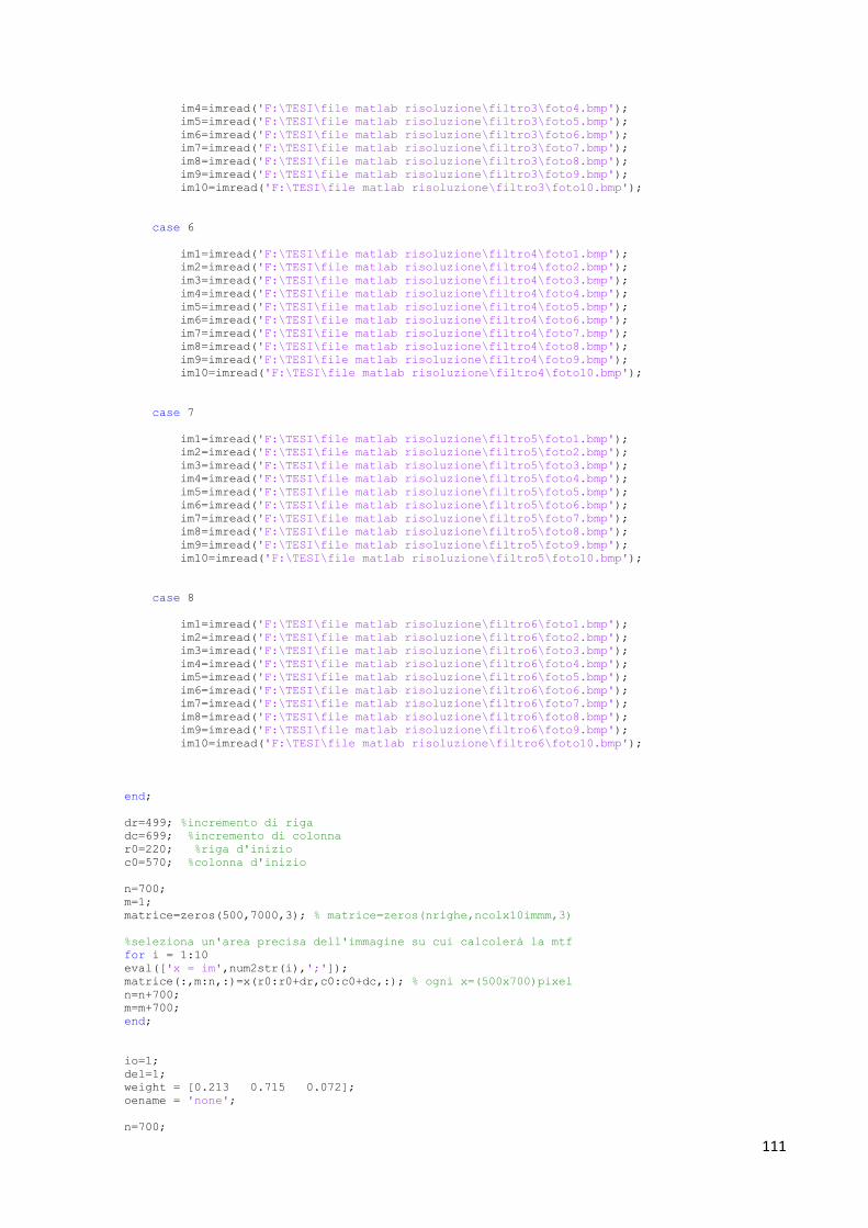
111
im4=imread('F:\TESI\file matlab risoluzione\filtro3\foto4.bmp');
im5=imread('F:\TESI\file matlab risoluzione\filtro3\foto5.bmp');
im6=imread('F:\TESI\file matlab risoluzione\filtro3\foto6.bmp');
im7=imread('F:\TESI\file matlab risoluzione\filtro3\foto7.bmp');
im8=imread('F:\TESI\file matlab risoluzione\filtro3\foto8.bmp');
im9=imread('F:\TESI\file matlab risoluzione\filtro3\foto9.bmp');
im10=imread('F:\TESI\file matlab risoluzione\filtro3\foto10.bmp');
case 6
im1=imread('F:\TESI\file matlab risoluzione\filtro4\foto1.bmp');
im2=imread('F:\TESI\file matlab risoluzione\filtro4\foto2.bmp');
im3=imread('F:\TESI\file matlab risoluzione\filtro4\foto3.bmp');
im4=imread('F:\TESI\file matlab risoluzione\filtro4\foto4.bmp');
im5=imread('F:\TESI\file matlab risoluzione\filtro4\foto5.bmp');
im6=imread('F:\TESI\file matlab risoluzione\filtro4\foto6.bmp');
im7=imread('F:\TESI\file matlab risoluzione\filtro4\foto7.bmp');
im8=imread('F:\TESI\file matlab risoluzione\filtro4\foto8.bmp');
im9=imread('F:\TESI\file matlab risoluzione\filtro4\foto9.bmp');
im10=imread('F:\TESI\file matlab risoluzione\filtro4\foto10.bmp');
case 7
im1=imread('F:\TESI\file matlab risoluzione\filtro5\foto1.bmp');
im2=imread('F:\TESI\file matlab risoluzione\filtro5\foto2.bmp');
im3=imread('F:\TESI\file matlab risoluzione\filtro5\foto3.bmp');
im4=imread('F:\TESI\file matlab risoluzione\filtro5\foto4.bmp');
im5=imread('F:\TESI\file matlab risoluzione\filtro5\foto5.bmp');
im6=imread('F:\TESI\file matlab risoluzione\filtro5\foto6.bmp');
im7=imread('F:\TESI\file matlab risoluzione\filtro5\foto7.bmp');
im8=imread('F:\TESI\file matlab risoluzione\filtro5\foto8.bmp');
im9=imread('F:\TESI\file matlab risoluzione\filtro5\foto9.bmp');
im10=imread('F:\TESI\file matlab risoluzione\filtro5\foto10.bmp');
case 8
im1=imread('F:\TESI\file matlab risoluzione\filtro6\foto1.bmp');
im2=imread('F:\TESI\file matlab risoluzione\filtro6\foto2.bmp');
im3=imread('F:\TESI\file matlab risoluzione\filtro6\foto3.bmp');
im4=imread('F:\TESI\file matlab risoluzione\filtro6\foto4.bmp');
im5=imread('F:\TESI\file matlab risoluzione\filtro6\foto5.bmp');
im6=imread('F:\TESI\file matlab risoluzione\filtro6\foto6.bmp');
im7=imread('F:\TESI\file matlab risoluzione\filtro6\foto7.bmp');
im8=imread('F:\TESI\file matlab risoluzione\filtro6\foto8.bmp');
im9=imread('F:\TESI\file matlab risoluzione\filtro6\foto9.bmp');
im10=imread('F:\TESI\file matlab risoluzione\filtro6\foto10.bmp');
end;
dr=499; %incremento di riga
dc=699; %incremento di colonna
r0=220; %riga d'inizio
c0=570; %colonna d'inizio
n=700;
m=1;
matrice=zeros(500,7000,3); % matrice=zeros(nrighe,ncolx10immm,3)
%seleziona un'area precisa dell'immagine su cui calcolerà la mtf
for i = 1:10
eval(['x = im',num2str(i),';']);
matrice(:,m:n,:)=x(r0:r0+dr,c0:c0+dc,:); % ogni x=(500x700)pixel
n=n+700;
m=m+700;
end;
io=1;
del=1;
weight = [0.213 0.715 0.072];
oename = 'none';
n=700;

112
m=1;
m_mtf=zeros(7000,4);
%calcolo della mtf con programma matlab sfrmat3
%la matrice m_mtf è a blocchi di 251 elementi impilati uno sopra l'altro.
%ogni blocco è un'immagine --> ho 10 blocchi perché ci sono 10 immagini
for j=1:10
a=matrice(:,m:n,:);
m_mtf(m:n,:) = sfrmat3(io, del, weight, a, oename);
m=n+1;
n=n+700;
end;
freq=m_mtf(1:700,1); % estraggo la prima colonna che corrisponde alle freq spaziali
mat_mtf=m_mtf(:,2:4); % seleziono le colonne 2,3,4 per creare la matrice con le sole mtf
xlswrite('matrice_mtf',m_mtf); %copio la matrice in un file excel
figure
plot(freq,m_mtf(1:700,2),'-r')
axis([0 0.5, 0 1])
xlabel('frequenza spaziale')
ylabel('SFR')
hold on
plot(freq,m_mtf(1:700,3),'-g')
hold on
plot(freq,m_mtf(1:700,4),'-b')
r=zeros(701,1);
g=zeros(701,1);
b=zeros(701,1);
rn=0;
gn=0;
bn=0;
%sommo i elementi analoghi di immagini diverse.Lo ripeto per ogni colore
for k=1:251
for p=0:9
rn=rn+mat_mtf(k+701*p,1);
gn=gn+mat_mtf(k+701*p,2);
bn=bn+mat_mtf(k+701*p,3);
end
r(k)=rn;
g(k)=gn;
b(k)=bn;
rn=0;
gn=0;
bn=0;
end;
%faccio la media e tengo separate le tre medie(una per ogni colore r,g,b)
red=r/10;
green=g/10;
blue=b/10;
mtf_mediata_sf=[red green blue];
xlswrite('matrice_mtf_mediata',mtf_mediata_sf);
Funzione “sfrmat3”
function [ris] = sfrmat3(io, del, weight, a, oename)
% MatLab function: sfrmat3 Slanted-edge Analysis for digital camera and scanner

113
% evaluation. Updated version of sfrmat2.
% [status, dat, fitme, esf, nbin, del2] = sfrmat3(io, del, weight, a, oecfname);
% From a selected edge area of an image, the program computes
% the ISO slanted edge SFR. Input file can be single or
% three-record file. Many image formats are supported. The image
% is displayed and a region of interest (ROI) can be chosen, or
% the entire field will be selected by not moving the mouse
% when defining an ROI (simple click). Either a vertical or horizontal
% edge features can be analized.
% Input arguments:
% io (optional)
% 0 = (default) R,G,B,Lum SFRs + edge location(s)
% = 'sfrmat2' R,G,B,Lum SFRs + edge location(s)but
% with the same calculations as the previous version, sfrmat2
% 1 = Non GUI usage with supplied data array
% del (optional) sampling interval in mm or pixels/inch
% If dx < 1 it is assumed to be sampling pitch in mm
% If io = 1 (see below, no GUI) and del is not specified,
% it is set equal to 1, so frequency is given in cy/pixel.
% weight (optiona) default 1 x 3 r,g,b weighs for luminance weighting
% a (required if io =1) an nxm or nxmx3 array of data
% oename optional name of oecf LUT file containing 3xn or 1xn array
%
% Returns:
% status = 0 if normal execution
% dat = computed sfr data
% fitme = coefficients for the linear equations for the fit to
% edge locations for each color-record. For a 3-record
% data file, fitme is a (4 x 3) array, with the last column
% being the color misregistration value (with green as
% reference).
% esf = supersampled edge-spread functin array
% nbin = binning factor used
% del2 = sampling interval for esf, from which the SFR spatial
% frequency sampling is was computed. This will be
% approximately 4 times the original image sampling.
%
%EXAMPLE USAGE:
% sfrmat3 file and ROI selection and
% sfrmat3(1) = GUI usage
% sfrmat3(0, del) = GUI usage with del as default sampling in mm
% or dpi
% sfrmat3(2, del, weight) = GUI usage with del as default sampling
% in mm or dpi and weight as default luminance
% weights
% sfrmat3(4, dat) = non-GUI usage for data array, dat, with default
% sampling and weights aplied (del =1,
% weights = [.3 .6 .1])
% [status, dat, fitme] = sfrmat3(4, del, weight, a, oecfdat);
% sfr and edge locations, are returned for data
% array dat using oecf array, oecfdat, with
% specified sampling interval and luminance weights
%
%Provided in support of digital imaging performance standards being development
%by the International Imaging Industry Association (i3a.org).
%
%Author: Peter Burns, 24 July 2009
% Copyright (c) 2009 Peter D. Burns, [email protected]
%******************************************************************
status = 0;
% defpath = path; % save original path
% home = pwd; % add current directory to path
% addpath(home);
% name = 'sfrmat3';
% version = '1.0';
% when = '24 July 2009';
%ITU-R Recommendation BT.709 weighting
% %guidefweight = ['0.213'
% '0.715'
% '0.072'];
%Previously used weighting
defweight = [0.213 0.715 0.072];
weight=defweight;
oecfdatflag = 0;
oldflag = 0;

114
nbin = 4;
%sflag = 0;
%pflag=0;
% switch nargin
%
% case 0
% io =0;
% del =1;
% weight = guidefweight;
% oename = 'none';
%
% case 1
% if isempty(io) ==1;
% io =0;
% else
% if ischar(io) == 1;
% test = 'sfrmat2';
% if strcmpi(io, test) == 1;
% oldflag = 1;
% defweight = [0.3 0.6 0.1];
% end
% io = 0;
% end
% end
% del = 1;
% weight = guidefweight;
% oename = 'none';
%
% case 2
% if isempty(io) == 1;
% io = 0;
% end
% if isempty(del) == 1;
% del = 1;
% end
% oename = 'none';
% case 3
% if isempty(io) == 1;
% io = 0;
% end
% if isempty(del) == 1;
% del = 1;
% if isempty(weigh) == 1
% weight = guidefweight;
% else wsize = size(weight);
% if wsize ~= [1, 3];
% weight = guidefweight;
% oename = 'none';
% end
% end
% end
%
% case 4
% if isempty(io) == 1;
% io = 0;
% elseif ischar(io) == 1;
% test = 'sfrmat2';
% if strcmpi(io, test) == 1;
% oldflag = 1;
% defweight = [0.3 0.6 0.1];
% end
% io = 1;
% end
%
% a = double(a);
%
% if isempty(del) == 1;
% del = 1;
% end
% if isempty(weight) == 1
% weight = guidefweight;
% else wsize = size(weight);
% if wsize ~= [1, 3];
% weight = guidefweight;
% oename = 'none';
% end
% end

115
%
% case 5
%
% disp(oename);
% oecfdatflag = 1;
% otherwise
% disp('Incorrect number or arguments. There should be 1 -5');
% status = 1;
% return
% end
%%%%%%%%%%%%%%%%%%%%%%%%%%%%%%%%%%%%%%%%%%%%%%%%%%%%%%%%%%%%%%%%%%%%%%
% if io ~= 0 & io ~= 1
% beep
% disp(['Input argument io shoud be 0 or 1, setting equal to 0'])
% io =0;
% end
%%%%%%%%%%%%%%%%%%%%%%%%%%%%%%%%%%%%%%%%%%%%%%%%%%%%%%%%%%%%%%%%%%%%%%%
% Suppresses interpreting of e.g. filenames
% set(0, 'DefaultTextInterpreter', 'none');
%
% if io ~= 1;
%
% swin = splash(name, version, when);
% Select file name for reading
% edit the next line to change the default path for input file selection
% drawnow;
%
% pause(.2)
% [status, atemp, ftype, pathname, f] = imageread;
%close(swin); drawnow;
% if status~=0
% disp('No file selected. To try again type: > sfrmat3');
% status = 1;
% return;
% end;
% filename = [pathname,f];
atemp=a;
[nlin npix ncol] = size(atemp);
% input sampling and luminance weights
% if ncol==1;
% del = inbox1;
% else
% [del, weight] = inbox3(del, guidefweight);
% end;
% % used for plotting and listing
if del==1;
funit = 'cy/pixel';
else funit = 'cy/mm';
end;
cname = class(atemp);
if strcmp(cname(1:5), 'uint1') == 1; % uint16
smax = 2^16-1;
elseif strcmp(cname(1:5), 'uint8') == 1;
smax = 255;
else
smax = 1e10;
end
% b=size(a);
% c=b(1)*b(2);
% roi=a(1:c);
a = double(a);
% extract Region of interest
clear atemp % *******************************
[nlow, nhigh, cstatus] = clipping(a, 0, smax, 0.005);
if cstatus ~=1;
disp('Fraction low data');
disp(nlow);
disp('Fraction high data');
116
disp(nhigh);
end;
if oecfdatflag == 1;
disp('Applying OECF look-up table');
[a, oestatus] = getoecf(a, oename); % Transforms a using OECF LUT from file chosen
end;
%%%%
% when io = 1
a= double(a);
if oecfdatflag ~= 0;
oecfdat=load(oename);
size(oecfdat);
[a, oestatus] = getoecf(a, oecfdat);
disp('oecfdat applied')
end
if del > 1
del = 25.4/del; % Assume input was in DPI convert to pitch in mm
end;
[nlin npix ncol] = size(a);
% Form luminance record using the weight vector for red, green and blue
if ncol ==3;
lum = zeros(nlin, npix);
lum = weight(1)*a(:,:,1) + weight(2)*a(:,:,2) + weight(3)*a(:,:,3);
cc = zeros(nlin, npix*4);
cc = [ a(:, :, 1), a(:, :, 2), a(:,:, 3), lum];
cc = reshape(cc,nlin,npix,4);
a = cc;
clear cc;
clear lum;
ncol = 4;
end;
% Rotate horizontal edge so it is vertical
% [a, nlin, npix, rflag] = rotatev(a); %sfrmat2 version based on dimensions
[a, nlin, npix, rflag] = rotatev2(a); %based on data values
loc = zeros(ncol, nlin);
fil1 = [0.5 -0.5];
fil2 = [0.5 0 -0.5];
% We Need 'positive' edge
tleft = sum(sum(a(:, 1:5, 1),2));
tright = sum(sum(a(:, npix-5:npix,1),2));
if tleft>tright;
fil1 = [-0.5 0.5];
fil2 = [-0.5 0 0.5];
end
% Test for low contrast edge;
test = abs( (tleft-tright)/(tleft+tright) );
if test < 0.2;
disp(' ** WARNING: Edge contrast is less that 20%, this can');
disp(' lead to high error in the SFR measurement.');
end;
fitme = zeros(ncol, 3);
slout = zeros(ncol, 1);
% Smoothing window for first part of edge location estimation -
% to be used on each line of ROI
win1 = ahamming(npix, (npix+1)/2); % Symmetric window
for color=1:ncol; % Loop for each color
%%%%
c = deriv1(a(:,:,color), nlin, npix, fil1);
% compute centroid for derivative array for each line in ROI. NOTE WINDOW array 'win'
for n=1:nlin
loc(color, n) = centroid( c(n, 1:npix )'.*win1) - 0.5; % -0.5 shift for FIR phase
end;

117
% clear c
fitme(color,1:2) = findedge(loc(color,:), nlin);
place = zeros(nlin,1);
for n=1:nlin;
place(n) = fitme(color,2) + fitme(color,1)*n;
win2 = ahamming(npix, place(n));
loc(color, n) = centroid( c(n, 1:npix )'.*win2) -0.5;
end;
fitme(color,1:2) = findedge(loc(color,:), nlin);
end; % End of loop for each color
summary{1} = ' '; % initialize
if io > 0;
midloc = zeros(ncol,1);
summary{1} = 'Edge location, slope'; % initialize
for i=1:ncol;
slout(i) = - 1./fitme(i,1); % slope is as normally defined in image coods.
if rflag==1, % positive flag if ROI was rotated
slout(i) = - fitme(i,1);
end;
% evaluate equation(s) at the middle line as edge location
midloc(i) = fitme(i,2) + fitme(i,1)*((nlin-1)/2);
summary{i+1} = [midloc(i), slout(i)];
end
%%%%%%%%%%%%%%%%%%%%%%%%%%%%%%%%%%%%%%%%%%%%%%%%%%%%%%%%%%%%%%%%%%%%%%%%%%
if ncol>2;
summary{1} = 'Edge location, slope, misregistration (second record, G, is reference)';
misreg = zeros(ncol,1);
for i=1:ncol;
misreg(i) = midloc(i) - midloc(2);
summary{i+1}=[midloc(i), slout(i), misreg(i)];
fitme(i,3) = misreg(i);
end;
if io == 5;
disp('Misregistration, with green as reference (R, G, B, Lum) = ');
for i = 1:ncol
fprintf('%10.4f\n', misreg(i))
end;
end % io ==5
end % ncol>2
end %************ end of check if io > 0
% Full linear fit is available as variable fitme. Note that the fit is for
% the projection onto the X-axis,
% x = fitme(color, 1) y + fitme(color, 2)
% so the slope is the inverse of the one that you may expect
% Limit number of lines to integer(npix*line slope as per ISO algorithm
% except if processing as 'sfrmat2'
if oldflag ~= 1;
% disp(['Input lines: ',num2str(nlin)])
nlin1 = round(floor(nlin*abs(fitme(1,1)))/abs(fitme(1,1)));
% disp(['Integer cycle lines: ',num2str(nlin1)])
a = a(1:nlin1, :, 1:ncol);
end
%%%%
vslope = fitme(1,1);
slope_deg= 180*atan(abs(vslope))/pi;
disp(['Edge angle: ',num2str(slope_deg, 3),' degrees'])
if slope_deg < 3.5
beep, warndlg(['High slope warning ',num2str(slope_deg,3),' degrees'], 'Watch it!')
end
%%%%
del2=0;
if oldflag ~= 1;
%Correct sampling inverval for sampling parallel to edge
delfac = cos(atan(vslope));
del = del*delfac;
del2 = del/nbin;

118
end
%%%%%%%%%%%%%%%%%%%%%%%%%%%%%%%%%%%%%%%%%%%%%%%%%%%%%%%%%%%%%%%%%%%%%%%%
ns = length(summary);
summary{ns+1} = [del, del2];
nn = floor(npix *nbin);
mtf = zeros(nn, ncol);
nn2 = floor(nn/2) + 1;
if oldflag ~=1;
disp('Derivative correction')
dcorr = fir2fix(nn2, 3); % dcorr corrects SFR for response of FIR filter
end
freq = zeros(nn, 1);
for n=1:nn;
freq(n) = nbin*(n-1)/(del*nn);
end;
freqlim = 1;
if nbin == 1;
freqlim = 2;
end
nn2out = round(nn2*freqlim/2);
nfreq = n/(2*del*nn); % half-sampling frequency
win = ahamming(nbin*npix,(nbin*npix+1)/2); % centered Hamming window
% ************** Large SFR loop for each color record
esf = zeros(nn,ncol);
for color=1:ncol
% project and bin data in 4x sampled array
[point, status] = project(a(:,:,color), loc(color, 1), fitme(color,1), nbin);
esf(:,color) = point;
% compute first derivative via FIR (1x3) filter fil
c = deriv1(point', 1, nn, fil2);
c = c';
psf(:,color) = c;
mid = centroid(c);
temp = cent(c, round(mid)); % shift array so it is centered
c = temp;
clear temp;
% apply window (symmetric Hamming)
c = win.*c;
%%%%
% Transform, scale and correct for FIR filter response
temp = abs(fft(c, nn));
mtf(1:nn2, color) = temp(1:nn2)/temp(1);
if oldflag ~=1;
mtf(1:nn2, color) = mtf(1:nn2, color).*dcorr;
end
%%%%%%%%%%%%%%%%%%%%%%%%%%%%%%%%%%%%%%%%%%%%%%%%%%%%%%%%%%%%%%%%%%%%%%%%
end; % color=1:ncol
dat = zeros(nn2out, ncol+1);
for i=1:nn2out;
dat(i,:) = [freq(i), mtf(i,:)];
ris(i,:)=dat(i,:);% aggiunto io (ele)
end;
ris=dat(2:701,1:4);
%
% xlswrite('myfile',ris);
%%%%%%%%%%%%%%%%%%%%%%%%%%%%%%%%%%%%%%%%
%Sampling efficiency
%Values used to report: note lowest (10%) is used for sampling efficiency
val = [0.1, 0.5];

119
[e, freqval, sfrval] = sampeff(dat, val, del, 0, 0);
%%%%%%%%%%%%%%%%%%%%%%%%%%%%%%%%%%%%%%%%
ns = length(summary);
summary{ns+1} = e;
if io ==1;
return
end
% Plot SFRs on same axes
if ncol >1;
sym{1} = [];
sym{1} = '--r';
sym{2} = '-g';
sym{3} = '-.b';
sym{4} = '*k';
ttext = filename;
legg = [{'r'},{'g'},{'b'},{'lum'}];
else
ttext = filename;
sym{1} = 'k';
end
screen = get(0, 'ScreenSize');
pos = round(centerfig(1, 0.6,0.6));
%%%%%%%%%%%%%%%%%%% GRAFICO
nn4 = floor(nn/8) + 1;
cc = [.5 .5 .8];
%%%%%%%%%%%%%%%%%%%%%%%%%%%% SALVATAGGIO DATI SFR
% defname = [pathname,'*.*'];
% [outfile,outpath]=uiputfile(defname,'File name to save results (.xlsm will be added)');
% foutfile=[outpath,outfile];
%
% if size(foutfile)==[1,2],
% if foutfile==[0,0],figure('Position',pos)
plot( freq( 1:nn2out), mtf(1:nn2out, 1), sym{1});
hold on;
title(ttext);
xlabel([' Frequency, ', funit]);
ylabel('SFR');
if ncol>1;
for n = 2:ncol-1;
plot( freq( 1:nn2out), mtf(1:nn2out, n), sym{n});
end;
ndel = round(nn2out/30);
plot( freq( 1:ndel:nn2out), mtf(1:ndel:nn2out, ncol), 'ok',...
freq( 1:nn2out), mtf(1:nn2out, ncol), 'k')
h=legend(['r ',num2str(e(1)),'%'],['g ',num2str(e(2)),'%'],...
['b ',num2str(e(3)),'%'],...
['L ',num2str(e(4)),'%']);
pos1 = get(h,'Position');
set(h,'Position', [0.97*pos1(1) 0.93*pos1(2) pos1(3) pos1(4)])
set(get(h,'title'),'String','Sampling Efficiency');
line([nfreq ,nfreq],[.05,0]);
else % (ncol ==1)
h = legend([num2str(e),'%']);
get(h,'Position');
pos1 = get(h,'Position');
set(h,'Position', [0.97*pos1(1) 0.93*pos1(2) pos1(3) pos1(4)])
set(get(h,'title'),'String','Sampling Efficiency');
line([nfreq ,nfreq],[.05,0]);
end % ncol>1
text(.95*nfreq,+.08,'Half-sampling'),
hold off;
axis([0 freq(round(0.75*nn2out)),0,max(max(mtf))]);
drawnow
% disp('Saving results: Cancelled')

120
% end;
% else
%
% nn = find(foutfile=='.');
% if isempty(nn) ==1;
% foutfile=[foutfile,'.xls'];
%
% end
%
%results2(dat,filename, roi, oename, summary, foutfile);
% end;
% Clean up
% Reset text interpretation
% set(0, 'DefaultTextInterpreter', 'tex')
% path(defpath); % Restore path to previous list
% cd(home); % Return to working directory
%
% disp(' * sfrmat3 finished *');
% r_med=mean(r);
% g_med=mean(g);
% b_med=mean(b);
%
% media= (r_med,g_med,b_med)
% for k=2:4
% for j=2:b(1)-1
% M(j-1,k-1)=ris(j,k)+ris(j+1,k);
% end
% end;
% for q=1:3
% media(1,q)=M(q)/(b(1)-1);
% end;
% %me=[media(i,:) 0 0]
% %ris(i,:)=[dat(i,:); me]
return;