Embed Size (px)
Citation preview
Vol. 105, No. 1 DUKE MATHEMATICAL JOURNAL © 2000
OSCILLATION AND VARIATION FOR THE HILBERTTRANSFORM
JAMES T. CAMPBELL, ROGER L. JONES, KARIN REINHOLD,and MÁTÉ WIERDL
1. Introduction. For eachε > 0, let
Hεf (x) = 1
π
∫|t |>ε
f (x− t)
tdt.
The Hilbert transform,Hf (x), is defined by
Hf (x) = limε→0+Hεf (x).
It is well known that this limit exists a.e. for allf ∈ Lp, 1 ≤ p < ∞. In thispaper, we will consider the oscillation and variation of this family of operators asε goes to zero, which gives extra information on their convergence as well as anestimate on the number ofλ-jumps they can have. For earlier results on oscillation andvariation operators in analysis and ergodic theory, including some historical remarksand applications, the reader may look in [2], [3], [5], [4], and [6].For each fixed sequence(ti) ↘ 0, we define the oscillation operator
�(H∗f
)(x) =
( ∞∑i=1
supti+1≤εi+1<εi≤ti
∣∣Hεif (x)−Hεi+1f (x)∣∣2)1/2
and the variation operator
��
(H∗f
)(x) = sup
(εi )↘0
( ∞∑i=1
∣∣Hεif (x)−Hεi+1f (x)∣∣�)1/� .
The main results of this paper are the following two theorems.
Theorem 1.1. The oscillation operator�(H∗f )(x) satisfies ‖�(H∗f )‖p ≤cp‖f ‖p for 1< p < ∞ andm{x : �(H∗f )(x) > λ} ≤ (c/λ)‖f ‖1.
Received 13 July 1999. Revision received 6 January 2000.2000Mathematics Subject Classification. Primary 42B20, 42B25; Secondary 42A50, 40A30.Jones’s work partially supported by National Science Foundation grant number DMS-9531526.Wierdl’s work partially supported by National Science Foundation grant number DMS-9500577.
59
60 CAMPBELL, JONES, REINHOLD, AND WIERDL
Theorem 1.2. If � > 2, then the variation operator��(H∗f )(x) satisfies‖��(H∗f )‖p ≤ c(p,�)‖f ‖p for 1 < p < ∞ and m{x : ��(H∗f )(x) > λ} ≤(c(�)/λ)‖f ‖1.The first issue to address is whether the operator�� is well defined. Since we
are taking a supremum over such a large set of sequences, it is not obvious that theresulting operator is measurable. To deal with this, we first restrict(εk) to lie in somefinite set, prove a norm inequality that is independent of the set, and then enlarge theset. In this way, we obtain the result with(εk) restricted to a countable dense set, say,the rationals. The final result follows from the continuity properties of the operatorsinvolved.It is useful to have a second notation for the oscillation and variation of the family
of operators. Since both�(H∗f ) and��(H∗f ) are seminorms on the familyHεf ,we often denote�(H∗f )(x) by ‖H∗f (x)‖� and��(H∗f )(x) by ‖H∗f (x)‖v� . See[4] for further discussion of these seminorms.More generally, ifWε is a family of operators, we consider the oscillation operator
�(W∗f
)(x) = ∥∥W∗f (x)
∥∥�
=( ∞∑i=1
supti+1≤εi+1<εi≤ti
∣∣Wεif (x)−Wεi+1f (x)∣∣2)1/2 ,
where(ti) is a fixed decreasing sequence, and the variation operator
��
(W∗f
)(x) = ∥∥W∗f (x)
∥∥v�
= sup(εi )↘0
( ∞∑i=1
∣∣Wεif (x)−Wεi+1f (x)∣∣�)1/� .
We also study theλ-jump operator
�(Wε,f,λ,x
)= sup
{n ≥ 0 : such that there exists1< t1 ≤ s2< t2< · · · ≤ sn < tn
with the property that∣∣Wtif (x)−Wsif (x)
∣∣> λ, i = 1,2, . . . ,n},
which gives the number ofλ-jumps of the familyWεf . Clearly, for a convergentfamily, the number ofλ-jumps must be finite a.e. The size of�(Wε,f,λ,x) gives usinformation about how the familyWε converges. We prove the following theorem.
Theorem 1.3. If � > 2, then the operator�(Hε,f,λ,x) satisfies‖�(Hε,f,
λ, ·)1/�‖p ≤ c(p,�)‖f ‖p for 1< p < ∞, and ifn ≥ 1, we have
m{x : �(Hε,f,λ,x
)> n
}≤ c(�)
λn1/�‖f ‖1.
OSCILLATION 61
Define
Vk(H∗f
)(x) = sup
(εi )↘0
∑1/2k<εi+1<εi≤1/2k−1
∣∣Hεif (x)−Hεi+1f (x)∣∣21/2
,
where the supremum is taken over all decreasing sequences(εi). Define the “shortvariation operator”
SV(H∗f
)(x) =
( ∞∑k=−∞
(Vk(H∗f
)(x))2)1/2
.
As before, it is sometimes convenient to denote this operator by‖H∗f (x)‖sV . For afamily of operators,Wε , define
Vk(W∗f
)(x) = sup
(εi )↘0
∑1/2k<εi+1<εi≤1/2k−1
∣∣Wεif (x)−Wεi+1f (x)∣∣21/2
and
SV(W∗f
)(x) =
( ∞∑k=−∞
(Vk(W∗f
)(x))2)1/2
,
where again the supremum is taken over all decreasing sequences(εi).We also prove the following theorem.
Theorem 1.4. The short variation operatorSV satisfies‖SV (H∗f )‖p ≤ cp‖f ‖pfor 1< p < ∞ andm{x : SV (H∗f )(x) > λ} ≤ (c/λ)‖f ‖1.The paper is organized as follows. In Section 2, we prove some general results
for oscillation and variation norms of certain types of convolution operators. Theseare used in Section 3 to show that the oscillation and variation norms of the Hilberttransform are bounded operators onLp, 1< p < ∞. In Section 5, we prove that theoscillation and variation norms satisfy a weak type (1,1) inequality if the gaps are“short.” In Section 6, we show that the “long variation,” that is, gaps between dyadicterms, satisfies a weak (1,1) result. Finally, in Section 7, we complete the proof ofTheorems 1.1, 1.2, and 1.3 by combining the results for long variation and shortvariation, thus obtaining results for the full variation.
Remark 1.5. If we wanted to consider truncation both near zero and near in-finity, we could argue as in the case of truncation only near zero. That followssince
∫a<|t |<b(f (x− t)/t)dt = ∫
|t |>a(f (x− t)/t)dt−∫|t |>b(f (x− t)/d)dt . Hence,we can control truncation in both directions by a sum of two operators, each of whichcontrols the truncation only on the small end.
62 CAMPBELL, JONES, REINHOLD, AND WIERDL
Remark 1.6. The inequalities in Theorems 1.1 and 1.2 are not a consequence of ageneral convergence principle such as the Banach principle. Consider the followingsimple example. Forn ≥ 1, let
T2nf (x) = 1
ln(n+1)f (x) and T2n+1f (x) = −1ln(n+1)f (x).
It is clear thatTnf (x) converges to zero a.e. for allf ∈ Lp for anyp, 1≤ p ≤ ∞.However, for any� > 0, we haveV�(T!f )(x) = ∞ and�(T!f )(x) = ∞ wheneverf (x) �= 0.
Remark 1.7. In general, to obtain a variation result, we need to assume� > 2. Thisalready occurs in the case of martingales (see [7]) and in the case of differentiationoperators. We could also define the oscillation and short variation operators withexponents� ≥ 2, but these are dominated by the 2-oscillation (2-short variation,resp.), so there is no need to do so. For� < 2, the�-oscillation operator fails to be abounded operator on anyLp (with ti = 1/2i). See [1] for the case of differentiation.The argument presented there can be applied to the case considered here as well.
Remark 1.8. Throughout this paper,c andC, sometimes with additional parame-ters, represent constants. However, they may represent different constants from oneoccurrence to the next.
Remark 1.9. There are higher dimensional analogs of the results mentioned inthis paper. In particular, certain Calderón-Zygmund singular integrals inRd satisfysimilar estimates. These operators will be considered in a subsequent paper.
2. Oscillation and variation norms for certain convolution operators. In thissection, we prove some lemmas about the oscillation and variation norms of certainkinds of convolution operators. These are used in the later sections.
Lemma 2.1. Let B+(x) = χ[0,1](x), and let D+t (x) = (1/t)B+(x/t). Define
D+t f (x) = D+
t !f (x). Thus,D+t is the standard differentiation operator.
(1) For any fixed sequence(ti) ↘ 0, the operator�(D+∗ ) is weak type (1,1) andstrong-type(p,p) for 1< p < ∞.(2) For � > 2, the operator��(D
+∗ ) is weak type (1,1) and strong type(p,p) for1< p < ∞.(3)The operatorSV (D+∗ ) is weak type (1,1) and strong type(p,p) for 1< p < ∞.
Proof. For the special casep = 2, see Bourgain [2]. For other values ofp, 1≤p < ∞, see [4] for a proof in the discrete case. (See [4, Theorem 2.13] forp = 2,[4, Theorem 3.6] for the weak (1,1) result, and [4, Theorem 4.4] for the BMO resultthat allows the interpolation to get the remaining values ofp.) The discrete case easilyimplies the continuous case. To see this, first consider the operators with the additionalrestriction that, for a fixed choice ofn ∈ Z+ and a fixedJ ∈ Z+, the differentiationlengths are selected from the set{r/2n : r ∈ Z}, and at mostJ terms are in the sum
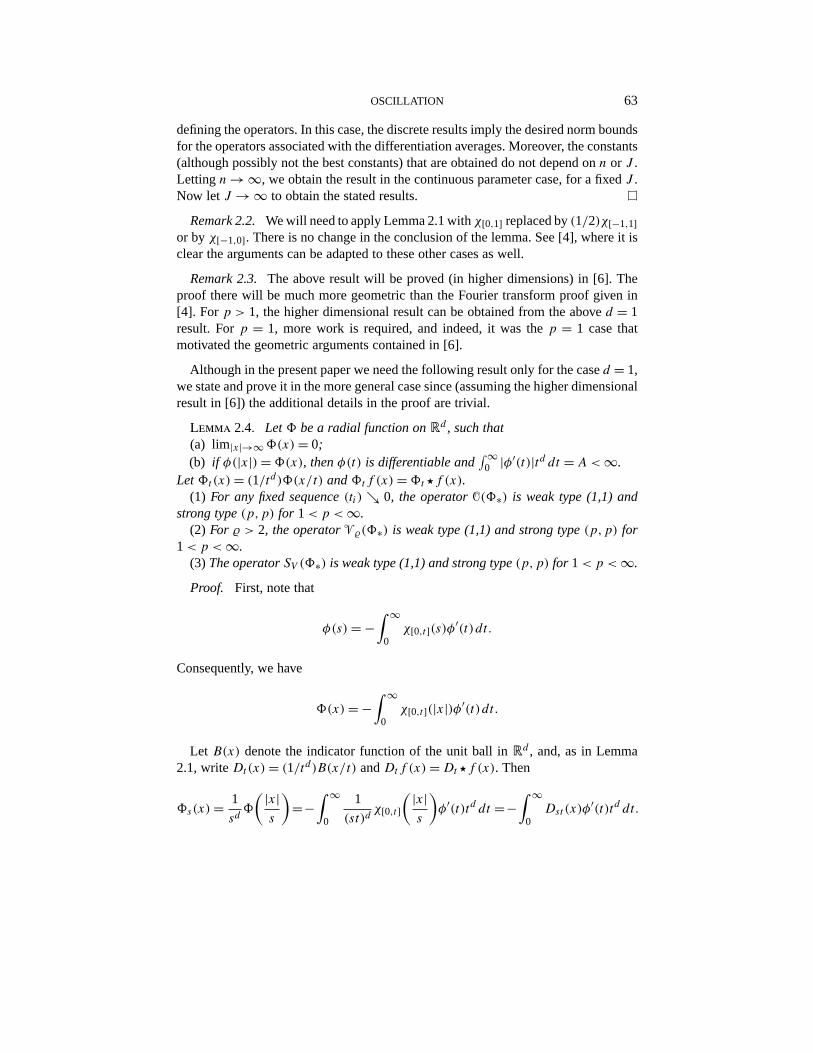
OSCILLATION 63
defining the operators. In this case, the discrete results imply the desired norm boundsfor the operators associated with the differentiation averages. Moreover, the constants(although possibly not the best constants) that are obtained do not depend onn or J .Lettingn → ∞, we obtain the result in the continuous parameter case, for a fixedJ .Now let J → ∞ to obtain the stated results.
Remark 2.2.Wewill need to apply Lemma 2.1 withχ[0,1] replaced by(1/2)χ[−1,1]or byχ[−1,0]. There is no change in the conclusion of the lemma. See [4], where it isclear the arguments can be adapted to these other cases as well.
Remark 2.3. The above result will be proved (in higher dimensions) in [6]. Theproof there will be much more geometric than the Fourier transform proof given in[4]. For p > 1, the higher dimensional result can be obtained from the aboved = 1result. Forp = 1, more work is required, and indeed, it was thep = 1 case thatmotivated the geometric arguments contained in [6].
Although in the present paper we need the following result only for the cased = 1,we state and prove it in the more general case since (assuming the higher dimensionalresult in [6]) the additional details in the proof are trivial.
Lemma 2.4. Let( be a radial function onRd , such that(a) lim|x|→∞((x) = 0;(b) if φ(|x|) = ((x), thenφ(t) is differentiable and
∫∞0 |φ′(t)|td dt = A< ∞.
Let(t(x) = (1/td)((x/t) and(tf (x) = (t !f (x).(1) For any fixed sequence(ti) ↘ 0, the operator�((∗) is weak type (1,1) and
strong type(p,p) for 1< p < ∞.(2) For � > 2, the operator��((∗) is weak type (1,1) and strong type(p,p) for
1< p < ∞.(3) The operatorSV ((∗) is weak type (1,1) and strong type(p,p) for 1< p < ∞.
Proof. First, note that
φ(s) = −∫ ∞
0χ[0,t](s)φ′(t)dt.
Consequently, we have
((x) = −∫ ∞
0χ[0,t](|x|)φ′(t)dt.
Let B(x) denote the indicator function of the unit ball inRd , and, as in Lemma2.1, writeDt(x) = (1/td)B(x/t) andDtf (x) = Dt !f (x). Then
(s(x) = 1
sd(
( |x|s
)=−
∫ ∞
0
1
(st)dχ[0,t]
( |x|s
)φ′(t)td dt =−
∫ ∞
0Dst (x)φ
′(t)td dt.
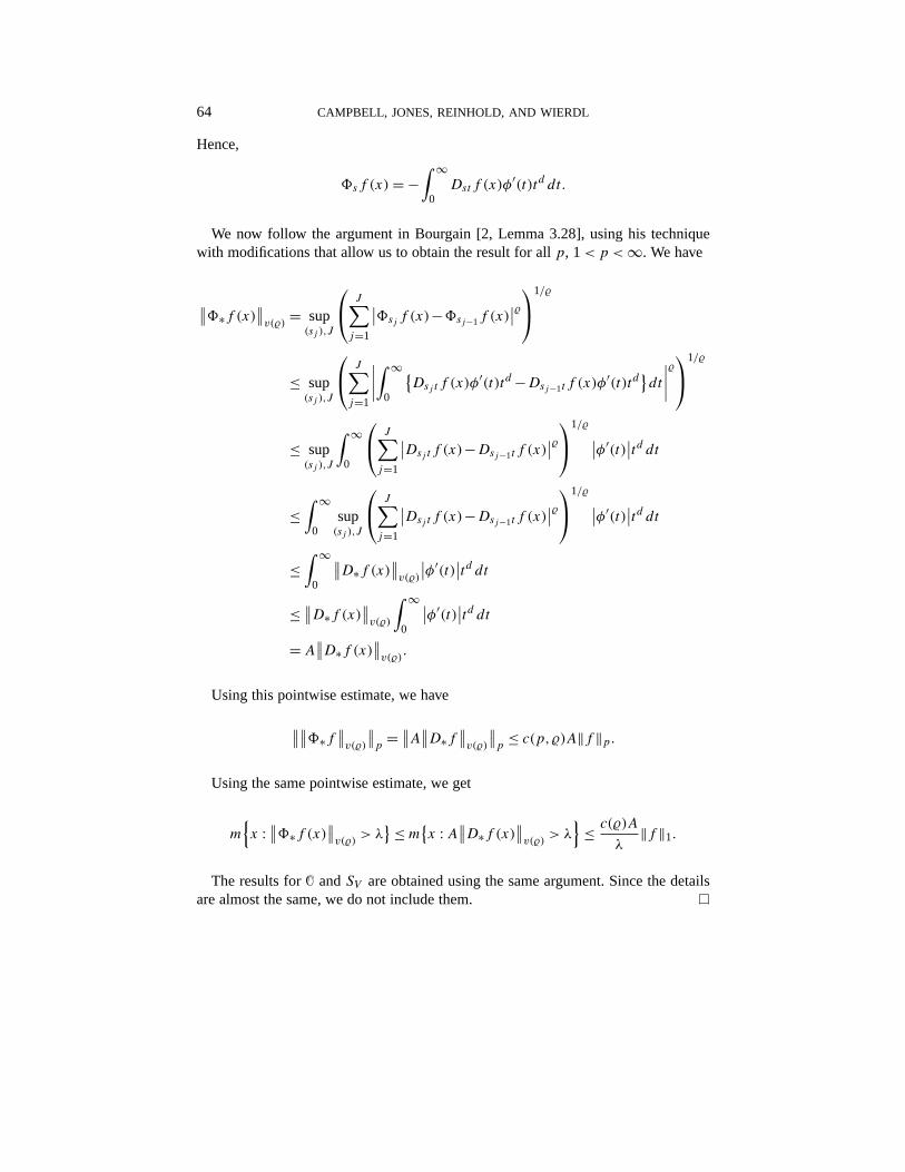
64 CAMPBELL, JONES, REINHOLD, AND WIERDL
Hence,
(sf (x) = −∫ ∞
0Dstf (x)φ
′(t)td dt.
We now follow the argument in Bourgain [2, Lemma 3.28], using his techniquewith modifications that allow us to obtain the result for allp, 1< p < ∞. We have
∥∥(∗f (x)∥∥v(�)
= sup(sj ),J
J∑j=1
∣∣(sj f (x)−(sj−1f (x)∣∣�1/�
≤ sup(sj ),J
J∑j=1
∣∣∣∣∫ ∞
0
{Dsj tf (x)φ
′(t)td −Dsj−1t f (x)φ′(t)td
}dt
∣∣∣∣�1/�
≤ sup(sj ),J
∫ ∞
0
J∑j=1
∣∣Dsj tf (x)−Dsj−1t f (x)∣∣�1/� ∣∣φ′(t)
∣∣td dt
≤∫ ∞
0sup(sj ),J
J∑j=1
∣∣Dsj tf (x)−Dsj−1t f (x)∣∣�1/� ∣∣φ′(t)
∣∣td dt≤∫ ∞
0
∥∥D∗f (x)∥∥v(�)
∣∣φ′(t)∣∣td dt
≤ ∥∥D∗f (x)∥∥v(�)
∫ ∞
0
∣∣φ′(t)∣∣td dt
= A∥∥D∗f (x)
∥∥v(�)
.
Using this pointwise estimate, we have
∥∥∥∥(∗f∥∥v(�)
∥∥p
= ∥∥A∥∥D∗f∥∥v(�)
∥∥p
≤ c(p,�)A‖f ‖p.
Using the same pointwise estimate, we get
m{x : ∥∥(∗f (x)
∥∥v(�)
> λ}≤ m
{x : A∥∥D∗f (x)
∥∥v(�)
> λ}
≤ c(�)A
λ‖f ‖1.
The results for� andSV are obtained using the same argument. Since the detailsare almost the same, we do not include them.
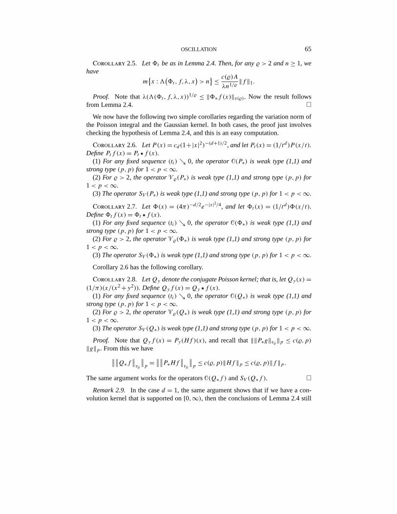
OSCILLATION 65
Corollary 2.5. Let(t be as in Lemma 2.4. Then, for any� > 2 andn ≥ 1, wehave
m{x : �((t,f,λ,x
)> n
}≤ c(�)A
λn1/�‖f ‖1.
Proof. Note thatλ(�((t ,f,λ,x))1/� ≤ ‖(∗f (x)‖v(�). Now the result follows
from Lemma 2.4.
We now have the following two simple corollaries regarding the variation norm ofthe Poisson integral and the Gaussian kernel. In both cases, the proof just involveschecking the hypothesis of Lemma 2.4, and this is an easy computation.
Corollary 2.6. LetP(x) = cd(1+|x|2)−(d+1)/2, and letPt(x) = (1/td)P (x/t).DefinePtf (x) = Pt !f (x).(1) For any fixed sequence(ti) ↘ 0, the operator�(P∗) is weak type (1,1) and
strong type(p,p) for 1< p < ∞.(2) For � > 2, the operator��(P∗) is weak type (1,1) and strong type(p,p) for
1< p < ∞.(3) The operatorSV (P∗) is weak type (1,1) and strong type(p,p) for 1< p < ∞.
Corollary 2.7. Let ((x) = (4π)−d/2e−|x|2/4, and let(t(x) = (1/td)((x/t).Define(tf (x) = (t !f (x).(1) For any fixed sequence(ti) ↘ 0, the operator�((∗) is weak type (1,1) and
strong type(p,p) for 1< p < ∞.(2) For � > 2, the operator��((∗) is weak type (1,1) and strong type(p,p) for
1< p < ∞.(3) The operatorSV ((∗) is weak type (1,1) and strong type(p,p) for 1< p < ∞.
Corollary 2.6 has the following corollary.
Corollary 2.8. LetQy denote the conjugate Poisson kernel; that is, letQy(x) =(1/π)(x/(x2+y2)). DefineQyf (x) = Qy !f (x).(1) For any fixed sequence(ti) ↘ 0, the operator�(Q∗) is weak type (1,1) and
strong type(p,p) for 1< p < ∞.(2) For � > 2, the operator��(Q∗) is weak type (1,1) and strong type(p,p) for
1< p < ∞.(3)The operatorSV (Q∗) is weak type (1,1) and strong type(p,p) for 1< p < ∞.
Proof. Note thatQyf (x) = Py(Hf )(x), and recall that‖‖P∗g‖v�‖p ≤ c(�,p)
‖g‖p. From this we have∥∥∥∥Q∗f∥∥v�
∥∥p
= ∥∥∥∥P∗Hf∥∥v�
∥∥p
≤ c(�,p)‖Hf ‖p ≤ c(�,p)‖f ‖p.
The same argument works for the operators�(Q∗f ) andSV (Q∗f ).
Remark 2.9. In the cased = 1, the same argument shows that if we have a con-volution kernel that is supported on[0,∞), then the conclusions of Lemma 2.4 still
66 CAMPBELL, JONES, REINHOLD, AND WIERDL
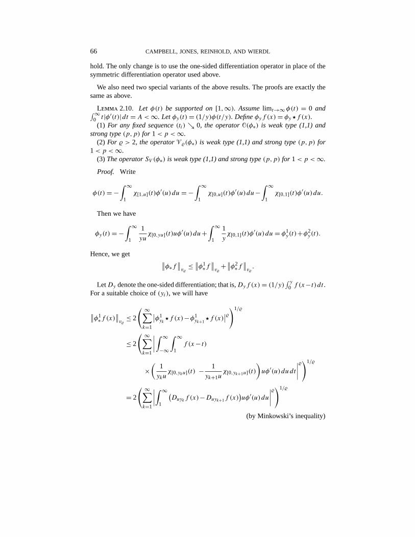
hold. The only change is to use the one-sided differentiation operator in place of thesymmetric differentiation operator used above.
We also need two special variants of the above results. The proofs are exactly thesame as above.
Lemma 2.10. Let φ(t) be supported on[1,∞). Assumelim t→∞φ(t) = 0 and∫∞0 t |φ′(t)|dt = A< ∞. Letφy(t) = (1/y)φ(t/y). Defineφyf (x) = φy !f (x).(1) For any fixed sequence(ti) ↘ 0, the operator�(φ∗) is weak type (1,1) and
strong type(p,p) for 1< p < ∞.(2) For � > 2, the operator��(φ∗) is weak type (1,1) and strong type(p,p) for
1< p < ∞.(3) The operatorSV (φ∗) is weak type (1,1) and strong type(p,p) for 1< p < ∞.
Proof. Write
φ(t) = −∫ ∞
1χ[1,u](t)φ′(u)du = −
∫ ∞
1χ[0,u](t)φ′(u)du−
∫ ∞
1χ[0,1](t)φ′(u)du.
Then we have
φy(t) = −∫ ∞
1
1
yuχ[0,yu](t)uφ′(u)du+
∫ ∞
1
1
yχ[0,1](t)φ′(u)du = φ1y(t)+φ2y(t).
Hence, we get ∥∥φ∗f∥∥v�
≤ ∥∥φ1∗f ∥∥v� +∥∥φ2∗f ∥∥v� .LetDy denote the one-sided differentiation; that is,Dyf (x) = (1/y)
∫ y0 f (x−t)dt .
For a suitable choice of(yi), we will have
∥∥φ1∗f (x)∥∥v� ≤ 2
( ∞∑k=1
∣∣φ1yk !f (x)−φ1yk+1 !f (x)∣∣�)1/�
≤ 2
( ∞∑k=1
∣∣∣∣∫ ∞
−∞
∫ ∞
1f (x− t)
×(1
ykuχ[0,yku](t) − 1
yk+1uχ[0,yk+1u](t)
)uφ′(u)dudt
∣∣∣∣�)1/�
= 2
( ∞∑k=1
∣∣∣∣∫ ∞
1
(Duykf (x)−Duyk+1f (x)
)uφ′(u)du
∣∣∣∣�)1/�
(by Minkowski’s inequality)
OSCILLATION 67
≤ 2∫ ∞
1
( ∞∑k=1
∣∣Dykuf (x)−Dyk+1uf (x)∣∣�)1/� u∣∣φ′(u)
∣∣du≤ 2
∫ ∞
1
∥∥D∗f (x)∥∥v�u∣∣φ′(u)
∣∣du≤ c
∥∥D∗f (x)∥∥v�.
Since we already know that‖‖D∗f ‖v�‖p≤c(p,�)‖f ‖p and thatm{x : ‖D∗f ‖v� >λ} ≤ (c(�)/λ)‖f ‖1, we are done with this piece.The argument for the second piece,‖φ2∗f ‖v� , is similar. The oscillation operator
and the short variation operator are handled in the same way. The details are left forthe reader.
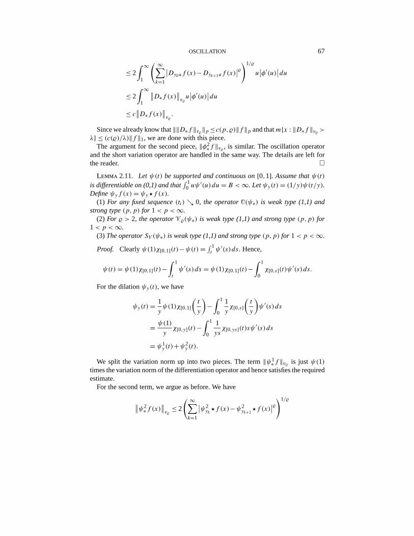
Lemma 2.11. Letψ(t) be supported and continuous on[0,1]. Assume thatψ(t)is differentiable on (0,1) and that
∫ 10 uψ
′(u)du = B < ∞. Letψy(t) = (1/y)ψ(t/y).Defineψyf (x) = ψy !f (x).(1) For any fixed sequence(ti) ↘ 0, the operator�(ψ∗) is weak type (1,1) and
strong type(p,p) for 1< p < ∞.(2) For � > 2, the operator��(ψ∗) is weak type (1,1) and strong type(p,p) for
1< p < ∞.(3) The operatorSV (ψ∗) is weak type (1,1) and strong type(p,p) for 1< p < ∞.
Proof. Clearlyψ(1)χ[0,1](t)−ψ(t) = ∫ 1tψ ′(s)ds. Hence,
ψ(t) = ψ(1)χ[0,1](t)−∫ 1
t
ψ ′(s)ds = ψ(1)χ[0,1](t)−∫ 1
0χ[0,s](t)ψ ′(s)ds.
For the dilationψy(t), we have
ψy(t) = 1
yψ(1)χ[0,1]
(t
y
)−∫ 1
0
1
yχ[0,s]
(t
y
)ψ ′(s)ds
= ψ(1)
yχ[0,y](t)−
∫ 1
0
1
ysχ[0,ys](t)sψ ′(s)ds
= ψ1y (t)+ψ2
y (t).
We split the variation norm up into two pieces. The term‖ψ1∗f ‖v� is justψ(1)times the variation norm of the differentiation operator and hence satisfies the requiredestimate.For the second term, we argue as before. We have
∥∥ψ2∗f (x)∥∥v�
≤ 2
( ∞∑k=1
∣∣ψ2yk!f (x)−ψ2
yk+1 !f (x)∣∣�)1/�
68 CAMPBELL, JONES, REINHOLD, AND WIERDL
= 2
( ∞∑k=1
∣∣∣∣∫ ∞
−∞
∫ 1
0f (x− t)
×(1
ykuχ[0,yku](t) − 1
yk+1uχ[0,yk+1u](t)
)uψ ′(u)dudt
∣∣∣∣�)1/�
= 2
( ∞∑k=1
∣∣∣∣∫ 1
0
(Duykf (x)−Duyk+1f (x)
)uψ ′(u)du
∣∣∣∣�)1/�
≤ 2∫ 1
0
( ∞∑k=1
∣∣Dykuf (x)−Dyk+1uf (x)∣∣�)1/� uψ ′(u)du
≤ 2∫ 1
0
∥∥D∗f (x)∥∥v�uψ ′(u)du
≤ c∥∥D∗f (x)
∥∥v�.
As before, we already know the operator‖D∗f (x)‖v� satisfies the required es-timates. The same argument works for both the oscillation operator and the shortvariation operators.
3. TheLp result for the Hilbert transform. In this section, we use the resultsof the prior section to establish theLp inequalities, 1< p < ∞ for Theorems 1.1 and1.2. In particular, we prove that for 1< p < ∞,
∥∥�(H∗f
)∥∥p
≤ cp‖f ‖p;
that for� > 2 and 1< p < ∞,
∥∥∥∥H∗f∥∥v�
∥∥p
≤ c�‖f ‖p;
and that for 1< p < ∞, ∥∥∥∥H∗f∥∥sv
∥∥p
≤ c‖f ‖p.
Proof. We actually prove only the result for the variation operator, the proofs forthe other two operators being exactly the same. Let
Qyf (x) = 1
π
∫ ∞
−∞f (x− t)
t
t2+y2dt
denote the conjugate Poisson kernel.
OSCILLATION 69
By the triangle inequality, we have
∥∥H∗f (x)∥∥v�
= ∥∥H∗f (x)−Q∗f (x)∥∥v�
+∥∥Q∗f (x)∥∥v�.
By Corollary 2.8, we see it is enough to control‖H∗f (x)−Q∗f (x)‖v� .Fix f ∈ Lp(R), x ∈R, andy > 0. We write
Hyf (x)−Qyf (x)
= 1
π
∫|t |>y
f (x− t)
(1
t− t
t2+y2
)dt− 1
π
∫|t |<y
f (x− t)t
t2+y2dt
= 1
π
∫ ∞
y
f (x− t)
(1
t− t
t2+y2
)dt− 1
π
∫ ∞
y
f (x+ t)
(1
t− t
t2+y2
)dt
− 1
π
∫ y
0f (x− t)
t
t2+y2dt+ 1
π
∫ y
0f (x+ t)
t
t2+y2dt
= A+y f (x)−A−
y f (x)−Gy+f (x)+G−y f (x).
We show that‖‖A+∗ f (x)‖v�‖p ≤ c�‖f ‖p and that‖‖G+∗ f (x)‖v�‖p ≤ c�‖f ‖p. Itis clear that similar estimates also hold for the associated operatorsA−
y f andG−y f .
Hence, the proof for��(Hf ) will be complete.The idea is to write the operators we need to study as a combination of differenti-
ation operators.Letφ(t) = (1/π)(1/t (t2+1))χ{t≥1}, and letψ(t) = (1/π)(t/t2+1)χ[0,1](t). Then
φy(t) = (1/y)φ(t/y) = (1/π)(y2/t (t2+y2))χ{t≥y} and ψy(t) = (1/y)ψ(t/y) =(1/π)(t/t2+y2)χ[0,y](t). Note thatA+
y f (x) = f !φy(x) andG+y f (x) = f !ψy(x).
We can now apply the results from Section 2 to complete the argument for each ofthese pieces.
4. Some necessary lemmas.In this section, we state some of the key lemmas thatwe need in the proof of the weak type (1,1) results. The first lemma is the Calderón-Zygmund decomposition. This decomposition allows us to break up a function intotwo pieces. One piece can be handled byL2 techniques. The second piece, which issupported on a small set, has mean value zero on each of the intervals that make upthe support.
Lemma 4.1 (Calderón-Zygmund decomposition). Anyf ∈ L1(R) can be writtenin the formf = g+b, where(1) ‖g‖2
L2≤ ‖f ‖
L1;
(2) b =∑j bj , where eachbj satisfies
(a) for somen, bj is supported in a dyadic intervalBj ∈ Ln;(b)
∫R bj (x) = 0 for eachj ;
70 CAMPBELL, JONES, REINHOLD, AND WIERDL
(c) ‖bj‖L1 ≤ 3|Bj |;(d)
∑j |Bj | ≤ ‖f ‖
L1, where|Bj | denotes the length of the intervalBj .
Since the Calderón-Zygmund decomposition is a standard tool in harmonic analy-sis, we do not include a proof. See Stein [8, pp. 17–19] or Torchinsky [9, pp. 84–85]for details.We also need the following almost orthogonality lemma. The use of almost orthog-
onality is a standard tool to proveL2 inequalities. Our use of the lemma to prove anL1 inequality is somewhat unusual. We use Lemma 4.2 and theL2 information it pro-vides to handle the functionb that occurs in the Calderón-Zygmund decomposition.See [6] for a similar application of this technique.
Lemma 4.2. Let(dn) be a sequence, and let(hk,n) be a double sequence of vectorsin a normed space(B,‖·‖). Let (σ (j))j∈Z be a sequence of positive numbers withw =∑
j σ (j) < ∞. Suppose that
∥∥hk,n∥∥ ≤ σ(n−k)‖dn‖ (4.1)
for everyn,k.Then we have
∑k
∥∥∥∥∑n
hk,n
∥∥∥∥2
≤ w2 ·∑n
‖dn‖2.
Proof. Clearly,
∥∥∥∥∥∑n
hk,n
∥∥∥∥∥ ≤∑n
∥∥hk,n∥∥ =∑n
σ 1/2(n−k) ·σ−1/2(n−k) ·∥∥hk,n∥∥ .Applying Cauchy’s inequality and (4.1), we have
∥∥∥∥∥∑n
hk,n
∥∥∥∥∥ ≤(∑
n
σ (n−k)
)1/2·(∑
n
σ (n−k) ·‖dn‖2)1/2
=(w ·∑n
σ (n−k) ·‖dn‖2)1/2
.
Hence,
∑k
∥∥∥∥∥∑n
hk,n
∥∥∥∥∥2
≤ w ·∑k
∑n
σ (k−n) ·‖dn‖2
OSCILLATION 71
= w ·∑n
∑k
σ (n−k) ·‖dn‖2
= w2 ·∑n
‖dn‖2 ,
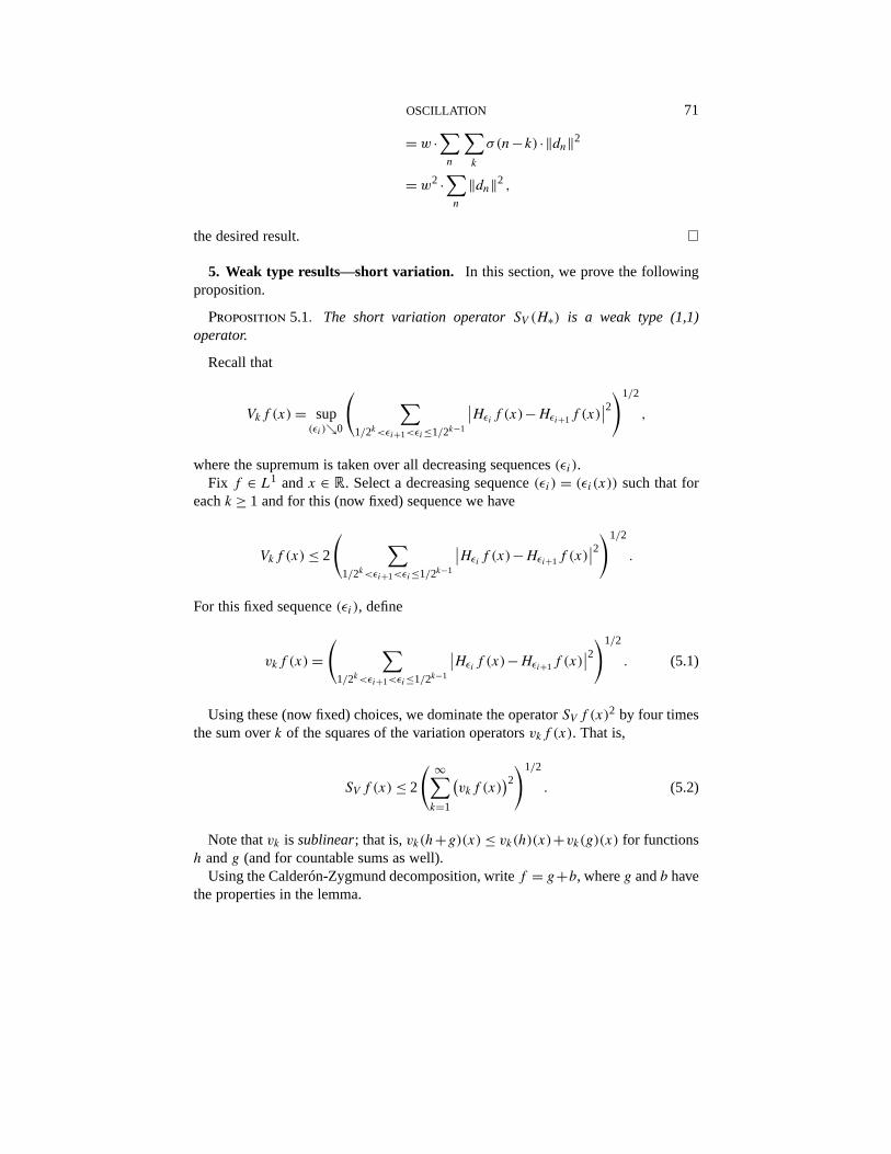
the desired result.
5. Weak type results—short variation. In this section, we prove the followingproposition.
Proposition 5.1. The short variation operatorSV (H∗) is a weak type (1,1)operator.
Recall that
Vkf (x) = sup(εi )↘0
( ∑1/2k<εi+1<εi≤1/2k−1
∣∣Hεif (x)−Hεi+1f (x)∣∣2)1/2 ,
where the supremum is taken over all decreasing sequences(εi).Fix f ∈ L1 andx ∈ R. Select a decreasing sequence(εi) = (εi(x)) such that for
eachk ≥ 1 and for this (now fixed) sequence we have
Vkf (x) ≤ 2
( ∑1/2k<εi+1<εi≤1/2k−1
∣∣Hεif (x)−Hεi+1f (x)∣∣2)1/2 .
For this fixed sequence(εi), define
vkf (x) =( ∑1/2k<εi+1<εi≤1/2k−1
∣∣Hεif (x)−Hεi+1f (x)∣∣2)1/2 . (5.1)
Using these (now fixed) choices, we dominate the operatorSV f (x)2 by four times
the sum overk of the squares of the variation operatorsvkf (x). That is,
SV f (x) ≤ 2
( ∞∑k=1
(vkf (x)
)2)1/2. (5.2)
Note thatvk is sublinear; that is,vk(h+g)(x) ≤ vk(h)(x)+vk(g)(x) for functionsh andg (and for countable sums as well).Using the Calderón-Zygmund decomposition, writef = g+b, whereg andb have
the properties in the lemma.
72 CAMPBELL, JONES, REINHOLD, AND WIERDL
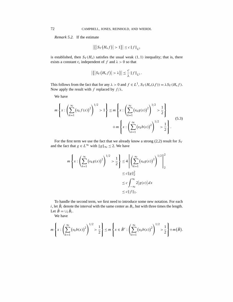
Remark 5.2. If the estimate
∣∣{∣∣SV (H∗f)∣∣> 1
}∣∣≤ c‖f ‖L1
is established, thenSV (H∗) satisfies the usual weak(1,1) inequality; that is, thereexists a constant c, independent off andλ > 0 so that
∣∣{∣∣SV (H∗f)∣∣> λ
}∣∣≤ c
λ‖f ‖
L1.
This follows from the fact that for anyλ > 0 andf ∈ L1, SV (H∗(λf )) = λSV (H∗f ).Now apply the result withf replaced byf/λ.
We have
m
x :
( ∞∑k=1
(vkf (x)
)2)1/2> 1
≤ m
x :
( ∞∑k=1
(vkg(x)
)2)1/2>1
2
+m
x :
( ∞∑k=1
(vkb(x)
)2)1/2>1
2
.
(5.3)
For the first term we use the fact that we already know a strong (2,2) result forSVand the fact thatg ∈ L∞ with ‖g‖∞ ≤ 2. We have
m
x :
( ∞∑k=1
(vkg(x)
)2)1/2>1
2
≤ 4
∥∥∥∥∥∥( ∞∑k=1
(vkg(x)
)2)1/2∥∥∥∥∥∥2
2
≤ c‖g‖22≤ c
∫ ∞
−∞2∣∣g(x)∣∣dx
≤ c‖f ‖1.
To handle the second term, we first need to introduce some new notation. For eachi, let Bi denote the interval with the same center asBi , but with three times the length.Let B = ∪i Bi .We have
m
x :
( ∞∑k=1
(vkb(x)
)2)1/2>1
2
≤ m
x ∈ Bc :
( ∞∑k=1
(vkb(x)
)2)1/2>1
2
+m
(B).
OSCILLATION 73
Sincem(B) ≤ 3∑
i m(Bi) ≤ 3‖f ‖1, it will be enough to study
m
x ∈ Bc :
( ∞∑k=1
(vkb(x)
)2)1/2>1
2
.
We have
m
x ∈ Bc :
( ∞∑k=1
(vkb(x)
)2)1/2>1
2
≤ 4
∫Bc
∞∑k=1
(vkb(x)
)2.
It will now be enough to prove∫Bc
∑k
∣∣νkb∣∣2 ≤ C ·∑j
∣∣Bj
∣∣. (5.4)
DefineLn to be the collection of intervals of the form[r/2n,(r+1)/2n) for someintegerr.Let us writeb =∑
n hn, where
hn =∑Bj∈Ln
bj
and
χn =∑Bj∈Ln
1Bj.
Note that ∑n
‖χn‖2L2 =∑n
‖χn‖L1 =∑j
∣∣Bj
∣∣.We will prove ∫
Bc
∣∣νkhn∣∣2 ≤ C ·2−|n−k| ·‖χn‖2L2 . (5.5)
Then, by applying the almost orthogonality lemma, Lemma 4.2, we conclude that∫Bc
∑k
∣∣vkhn∣∣2 ≤∑k
∑n
∫Bc
∣∣vkhn∣∣2 ≤∑n
‖χn‖22.
We consider two cases,n ≤ k andn > k.
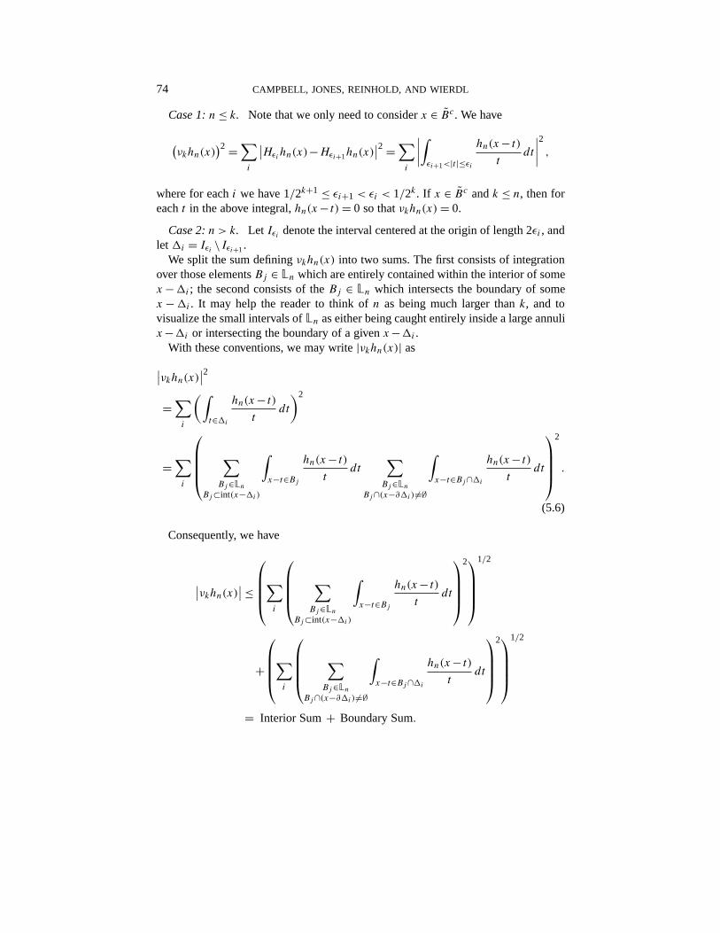
74 CAMPBELL, JONES, REINHOLD, AND WIERDL
Case 1:n ≤ k. Note that we only need to considerx ∈ Bc. We have
(νkhn(x)
)2 =∑i
∣∣Hεihn(x)−Hεi+1hn(x)∣∣2 =
∑i
∣∣∣∣∫εi+1<|t |≤εi
hn(x− t)
tdt
∣∣∣∣2
,
where for eachi we have 1/2k+1 ≤ εi+1 < εi < 1/2k. If x ∈ Bc andk ≤ n, then foreacht in the above integral,hn(x− t) = 0 so thatνkhn(x) = 0.
Case 2:n > k. Let Iεi denote the interval centered at the origin of length 2εi , andlet9i = Iεi \Iεi+1.We split the sum definingνkhn(x) into two sums. The first consists of integration
over those elementsBj ∈ Ln which are entirely contained within the interior of somex−9i ; the second consists of theBj ∈ Ln which intersects the boundary of somex −9i . It may help the reader to think ofn as being much larger thank, and tovisualize the small intervals ofLn as either being caught entirely inside a large annulix−9i or intersecting the boundary of a givenx−9i .With these conventions, we may write|νkhn(x)| as∣∣νkhn(x)∣∣2
=∑i
(∫t∈9i
hn(x− t)
tdt
)2
=∑i
∑Bj∈Ln
Bj⊂int(x−9i)
∫x−t∈Bj
hn(x− t)
tdt
∑Bj∈Ln
Bj∩(x−∂9i)�=∅
∫x−t∈Bj∩9i
hn(x− t)
tdt
2
.
(5.6)
Consequently, we have
∣∣νkhn(x)∣∣≤∑i
∑Bj∈Ln
Bj⊂int(x−9i)
∫x−t∈Bj
hn(x− t)
tdt
21/2
+
∑i
∑Bj∈Ln
Bj∩(x−∂9i)�=∅
∫x−t∈Bj∩9i
hn(x− t)
tdt
21/2
= Interior Sum+ Boundary Sum.
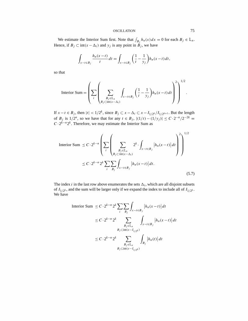
OSCILLATION 75
We estimate the Interior Sum first. Note that∫Bjhn(x)dx = 0 for eachBj ∈ Ln.
Hence, ifBj ⊂ int(x−9i) andyj is any point inBj , we have
∫x−t∈Bj
hn(x− t)
tdt =
∫x−t∈Bj
(1
t− 1
yj
)hn(x− t)dt,
so that
Interior Sum=
∑i
∑Bj∈Ln
Bj⊂int(x−9i)
∫x−t∈Bj
(1
t− 1
yj
)hn(x− t)dt
21/2
.
If x− t ∈ Bj , then|t | < 1/2k, sinceBj ⊂ x−9i ⊂ x−I1/2k /I1/2k+1. But the lengthof Bj is 1/2n, so we have that for anyt ∈ Bj , |(1/t)− (1/yj )| ≤ C ·2−n/2−2k =C ·2k−n2k. Therefore, we may estimate the Interior Sum as
Interior Sum≤ C ·2k−n
∑i
∑Bj∈Ln
Bj⊂ int(x−9i)
2k ·∫x−t∈Bj
∣∣hn(x− t)∣∣dt21/2
≤ C ·2k−n2k∑i
∑Bj
∫x−t∈Bj
∣∣hn(x− t)∣∣dt.
(5.7)
The indexi in the last row above enumerates the sets9i , which are all disjoint subsetsof I1/2k , and the sum will be larger only if we expand the index to include all ofI1/2k .We have
Interior Sum≤ C ·2k−n2k∑i
∑Bj
∫x−t∈Bj
∣∣hn(x− t)∣∣dt
≤ C ·2k−n2k∑Bj∈Ln
Bj⊂int(x−I1/2k )
∫x−t∈Bj
∣∣hn(x− t)∣∣dt
≤ C ·2k−n2k∑Bj∈Ln
Bj⊂int(x−I1/2k )
∫Bj
∣∣hn(t)∣∣dt
76 CAMPBELL, JONES, REINHOLD, AND WIERDL
≤ C ·2k−n2k∑Bj∈Ln
Bj⊂ int(x−I1/2k )
|Bj |
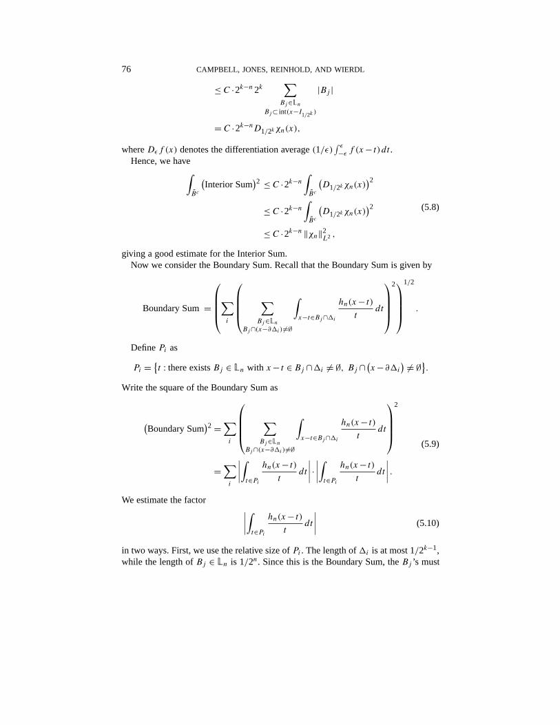
= C ·2k−nD1/2kχn(x),
whereDεf (x) denotes the differentiation average(1/ε)∫ ε−ε
f (x− t)dt .Hence, we have∫
Bc
(Interior Sum
)2 ≤ C ·2k−n
∫Bc
(D1/2kχn(x)
)2≤ C ·2k−n
∫Bc
(D1/2kχn(x)
)2≤ C ·2k−n ‖χn‖2L2 ,
(5.8)
giving a good estimate for the Interior Sum.Now we consider the Boundary Sum. Recall that the Boundary Sum is given by
Boundary Sum=
∑i
∑Bj∈Ln
Bj∩(x−∂9i)�=∅
∫x−t∈Bj∩9i
hn(x− t)
tdt
21/2
.
DefinePi as
Pi = {t : there existsBj ∈ Ln with x− t ∈ Bj ∩9i �= ∅, Bj ∩(x−∂9i
) �= ∅}.Write the square of the Boundary Sum as
(Boundary Sum
)2 =∑i
∑Bj∈Ln
Bj∩(x−∂9i)�=∅
∫x−t∈Bj∩9i
hn(x− t)
tdt
2
=∑i
∣∣∣∣∫t∈Pi
hn(x− t)
tdt
∣∣∣∣ ·∣∣∣∣∫t∈Pi
hn(x− t)
tdt
∣∣∣∣ .(5.9)
We estimate the factor ∣∣∣∣∫t∈Pi
hn(x− t)
tdt
∣∣∣∣ (5.10)
in two ways. First, we use the relative size ofPi . The length of9i is at most 1/2k−1,while the length ofBj ∈ Ln is 1/2n. Since this is the Boundary Sum, theBj ’s must
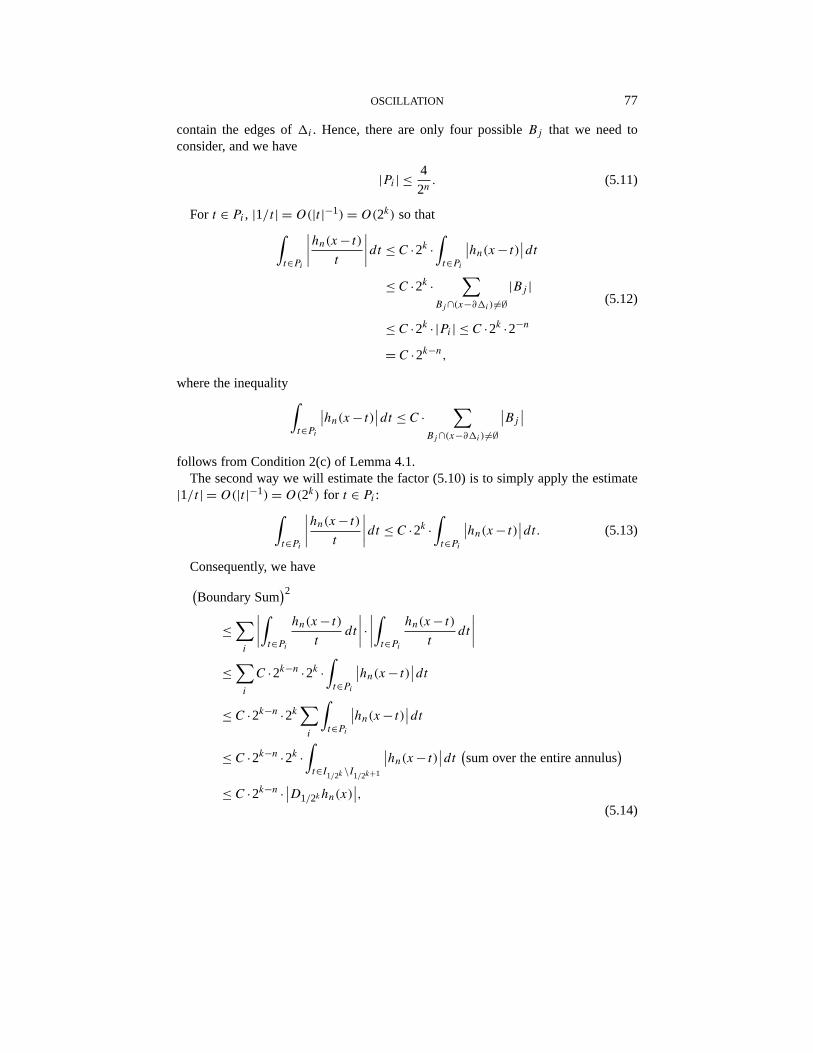
OSCILLATION 77
contain the edges of9i . Hence, there are only four possibleBj that we need toconsider, and we have
|Pi | ≤ 4
2n. (5.11)
For t ∈ Pi , |1/t | = O(|t |−1) = O(2k) so that∫t∈Pi
∣∣∣∣hn(x− t)
t
∣∣∣∣dt ≤ C ·2k ·∫t∈Pi
∣∣hn(x− t)∣∣dt
≤ C ·2k ·∑
Bj∩(x−∂9i)�=∅|Bj |
≤ C ·2k · |Pi | ≤ C ·2k ·2−n
= C ·2k−n,
(5.12)
where the inequality∫t∈Pi
∣∣hn(x− t)∣∣dt ≤ C ·
∑Bj∩(x−∂9i)�=∅
∣∣Bj
∣∣follows from Condition 2(c) of Lemma 4.1.The second way we will estimate the factor (5.10) is to simply apply the estimate
|1/t | = O(|t |−1) = O(2k) for t ∈ Pi :∫t∈Pi
∣∣∣∣hn(x− t)
t
∣∣∣∣dt ≤ C ·2k ·∫t∈Pi
∣∣hn(x− t)∣∣dt. (5.13)
Consequently, we have(Boundary Sum
)2≤∑i
∣∣∣∣∫t∈Pi
hn(x− t)
tdt
∣∣∣∣ ·∣∣∣∣∫t∈Pi
hn(x− t)
tdt
∣∣∣∣≤∑i
C ·2k−n ·2k ·∫t∈Pi
∣∣hn(x− t)∣∣dt
≤ C ·2k−n ·2k∑i
∫t∈Pi
∣∣hn(x− t)∣∣dt
≤ C ·2k−n ·2k ·∫t∈I1/2k \I1/2k+1
∣∣hn(x− t)∣∣dt (sum over the entire annulus
)≤ C ·2k−n · ∣∣D1/2khn(x)
∣∣,(5.14)
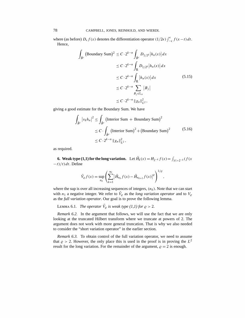
78 CAMPBELL, JONES, REINHOLD, AND WIERDL
where (as before)Dεf (x) denotes the differentiation operator(1/2ε)∫ ε−ε
f (x− t)dt .Hence, ∫
Bc
(Boundary Sum
)2 ≤ C ·2k−n
∫Bc
D1/2k∣∣hn(x)∣∣dx
≤ C ·2k−n
∫RD1/2k
∣∣hn(x)∣∣dx≤ C ·2k−n
∫R
∣∣hn(x)∣∣dx≤ C ·2k−n
∑Bj∈Ln
∣∣Bj
∣∣≤ C ·2k−n ‖χn‖2L2 ,
(5.15)
giving a good estimate for the Boundary Sum. We have∫Bc
∣∣νkhn∣∣2 ≤∫Bc
(Interior Sum+ Boundary Sum
)2≤ C ·
∫Bc
(Interior Sum
)2+(Boundary Sum)2≤ C ·2k−n ‖χn‖2L2 ,
(5.16)
as required.
6. Weak type (1,1) for the long variation. Let Hk(x) =H2−kf (x)= ∫|t |>2−k (f (x
− t)/t)dt . Define
V�f (x) = supnk
( ∞∑k=1
∣∣Hnkf (x)−Hnk+1f (x)∣∣�)1/� ,
where the sup is over all increasing sequences of integers,(nk). Note that we can startwith n1 a negative integer. We refer toV� as thelong variation operatorand toV�as thefull variation operator. Our goal is to prove the following lemma.
Lemma 6.1. The operatorV� is weak type (1,1) for� > 2.
Remark 6.2. In the argument that follows, we will use the fact that we are onlylooking at the truncated Hilbert transform where we truncate at powers of 2. Theargument does not work with more general truncation. That is why we also neededto consider the “short variation operator” in the earlier section.
Remark 6.3. To obtain control of the full variation operator, we need to assumethat � > 2. However, the only place this is used in the proof is in proving theL2
result for the long variation. For the remainder of the argument,� = 2 is enough.
OSCILLATION 79
Proof. We will apply the Calderón-Zygmund decomposition, Lemma 4.1. Usingthe notation in Lemma 4.1, we need to study the functionsg and b. The “goodfunction” g is handled as in the case of the short variation operator in Proposition 5.1since we already have anL2 result for the full variation and hence, in particular, forthe long variation. Following the argument in the proof of Proposition 5.1, and usingthe notation there, we see that it is enough to prove that∫
Bc
∣∣V�(H∗b)(x)∣∣dx ≤ c
∑i
|Bi |.
Since the<1 norm dominates the<� norm for� ≥ 1, it is in fact enough to provethat ∫
Bc
sup(nk)
∞∑k=1
∣∣Hnkb(x)−Hnk+1b(x)∣∣dx ≤ c
∑j
∣∣Bj
∣∣.This certainly follows if we prove for eachj that∫
Bcj
sup(nk)
∞∑k=1
∣∣Hnkbj (x)−Hnk+1bj (x)∣∣dx ≤ c
∣∣Bj
∣∣.Hence, proving this is our goal. For the remainder of the argument, fixj .Assume thatx ∈ Bc
j . There are two cases.
Case 1. There may be some exponentk0 so thatx−1/2k0 ∈ Bj or x+1/2k0 ∈ Bj ,depending on which side ofBj the pointx happens to be. Note that becausex ∈ Bc
j ,and because we are considering only dyadic truncation, there is at most one suchk0,and there may be none.Hence, forx ∈ Bc
j , if k0 is defined, we have
supnk
∞∑k=1
∣∣Hnkbj (x)−Hnk+1bj (x)∣∣dx
≤ ∣∣Hk0−1bj (x)−Hk0bj (x)∣∣+ ∣∣Hk0bj (x)−Hk0+1bj (x)
∣∣.We will consider only the first term. The other term is handled in the same way.
We have
∣∣Hk0−1bj (x)−Hk0bj (x)∣∣≤ ∣∣∣∣
∫|t |>2−k0+1
bj (x− t)
tdt
∣∣∣∣≤ c
d(x,Bj
)∥∥bj∥∥1≤ ∣∣Bj
∣∣ c
d(x,Bj
) ,whered(x,Bj ) denotes the distance fromx to the setBj .
80 CAMPBELL, JONES, REINHOLD, AND WIERDL
Let mj denote the midpoint ofBj . For eachn, let x+n and x−
n be defined byx+n −mj = 2n andx−
n −mj = −2n. Let
An =(x+n −
∣∣Bj
∣∣2
,x+n +
∣∣Bj
∣∣2
)∪(x−n −
∣∣Bj
∣∣2
,x−n +
∣∣Bj
∣∣2
).
Note thatk0 is defined only forx ∈ An for somen. Further,x ∈ Bcj implies
2n ≥ |Bj |. LetA = ∪2n≥|Bj |An.Using the above estimates, we have∫
A
∣∣Hk0−1bi(x)−Hk0bi(x)∣∣dx ≤
∑2n≥|Bj |
c∣∣Bj
∣∣ c2n∣∣Bj
∣∣≤ c∣∣Bj
∣∣,as required.
Case 2. We now deal with the pointsx ∈ Bc ∩Ac. However, for suchx, there isonly one term involved. For that term, one of the integrals does not contribute at all,since it starts beyond the support ofbj , and the other involves integration over all ofBj . For suchx, we have
��
(H∗bj
)(x) = ∣∣Hbj (x)
∣∣=∣∣∣∣∫Bcj
bj (t)
x− tdt
∣∣∣∣≤∣∣∣∣∫Bcj
bj (t)
x− t− bj (t)
x−mj
dt
∣∣∣∣≤∫Bcj
|bj (t)∣∣∣∣ c
∣∣Bj
∣∣d(x,Bj
)2 dt∣∣∣∣
≤ ∥∥bj∥∥1 c∣∣Bj
∣∣d(x,Bj
)2≤ c
∣∣Bj
∣∣2d(x,Bj
)2 .We can estimate the integral of this expression over the relevant set ofx’s by
∫Bcj∩Ac
sup(nk)
∞∑k=1
∣∣Hnkbj (x)−Hnk+1bj (x)∣∣dx ≤
∫Bcj
c∣∣Bj
∣∣2d(x,Bj
)2 dx ≤ c∣∣Bj
∣∣,as required.
OSCILLATION 81
7. Completion of the proof. We are now in a position to complete the proof ofTheorems 1.1, 1.2, and 1.3.
Proof of Theorem 1.2.Using Lemma 6.1, combined with the results about the“short variation operator,” Proposition 5.1, we show that��(H∗) is a weak type (1,1)operator.The idea is to introduce new operators,Rtf (x), defined byRtf (x) = Hkf (x),
where 2−(k+1) < t ≤ 2−k. Then we have
V�f (x) = supyk
( ∞∑k=1
∣∣Hykf (x)−Hyk+1f (x)∣∣�)1/�
≤ supyk
( ∞∑k=1
∣∣Hykf (x)−Rykf (x)+Rykf (x)−Ryk+1f (x)
+Ryk+1f (x)−Hyk+1f (x)∣∣�)1/�
≤ supyk
( ∞∑k=1
∣∣Hykf (x)−Rykf (x)+Ryk+1f (x)−Hyk+1f (x)∣∣�)1/�
+supyk
( ∞∑k=1
∣∣Rykf (x)−Ryk+1f (x)∣∣�)1/� .
The first term is controlled by the weak (1,1) result for the short variation.The second term is controlled byV�f , which, by Lemma 6.1, is a weak (1,1)
operator.We now have that��(H∗) is weak (1,1) and strong(p,p) for 1< p < ∞, com-
pleting the proof of Theorem 1.2.
Proof of Theorem 1.1.The idea is the same as in the proof above. We alreadyhave a strong(p,p) inequality. Thus we only need to prove a weak (1,1) result.Again, the Calderón-Zygmund decomposition is used. We already have control of the“good function,”g. For the “bad function,”b, we note that the only place we usedthe fact that� > 2 in the study of�� was in the proof of theL2 result. The restof the argument for the oscillation operator is exactly the same as the correspondingargument for the variation operator. The details are left to the reader.
Proof of Theorem 1.3.It is clear thatλ�(Hε,f,λ,x)1/� ≤ V�(H∗f )(x). Conse-
quently, we have
∥∥λ�(Hε,f,λ, ·)1/�∥∥
p≤ ∥∥V�(H∗f
)∥∥p
≤ c(p,�)‖f ‖p.
82 CAMPBELL, JONES, REINHOLD, AND WIERDL
Thus,‖�(Hε,f,λ, ·)1/�‖p ≤ (c(p,�)/λ)‖f ‖p. For the weak (1,1) result, we note thatm{x : �(Hε,f,λ,x
)> n
}≤ m{x : λ�(Hε,f,λ,x
)1/�> λn1/�
}≤ m
{x : V�
(H∗f
)(x) > λn1/�
}≤ c(�)
λn1/�‖f ‖1.
Fix α < β. Define the number ofupcrossingsN(Hε,f,α,β,x) by
N(Hε,f,α,β,x
)=max{n : there exists1< t1< s2< t2< · · · < sn < tn
such thatHsif (x) < α, Hti f (x) > β, i = 1,2, . . . ,n}.
Theorem 1.3 has the following immediate corollary regarding upcrossings.
Corollary 7.1. Letα < β. If � > 2, we have
∥∥N(Hε,f,α,β, ·)1/�∥∥
p≤ c(�)
β−α‖f ‖p
for 1< p < ∞, and
m{x : N(Hε,f,α,β,x
)> n
}≤ c(�)
(β−α)n1/�‖f ‖1.
Theorems 1.3 and 7.1 suggest the following conjectures.
Conjecture 7.2. The estimates in Theorem 1.3 can be improved to‖�(Hε,f,
λ, ·)1/2‖p ≤ (c(p)/λ)‖f ‖p, andm{x : �(Hε,f,λ,x) > n} ≤ (c/λn1/2)‖f ‖1.Conjecture 7.3. The estimates in Theorem 7.1 can be improved to‖N(Hε,f,
α,β, ·)‖p ≤ (c(p)/(β−α)n)‖f ‖p, and m{x : N(Hε,f,α,β,x) > n} ≤ (c/(β −α)n)‖f ‖1.In the case of analogous upcrossing andλ-jump operators for martingales, dif-
ferentiation averages, and ergodic averages, we know the improvements conjecturedabove are possible. However, our current techniques do not allow us to prove theseconjectures for the Hilbert transform.
References
[1] M. Akcoglu, R. L. Jones, and P. Schwartz, Variation in probability, ergodic theory andanalysis,Illinois J. Math.42 (1998), 154–177.
[2] J. Bourgain, Pointwise ergodic theorems for arithmetic sets,Inst. Hautes Études Sci. Publ.Math.69 (1989), 5–45.
[3] R. Jones, Ergodic theory and connections with analysis and probability,New York J. Math.3A(1997), 31–67, available from http://nyjm.albany.edu:8000/nyjm.html.
[4] R. Jones,R.Kaufmann, J. Rosenblatt, andM.Wierdl,Oscillation in ergodic theory,ErgodicTheory Dynam. Systems18 (1998), 889–935.
OSCILLATION 83
[5] R. Jones, I.Ostrovskii, and J.Rosenblatt,Square functions in ergodic theory,Ergodic TheoryDynam. Systems16 (1996), 267–305.
[6] R. Jones, J. Rosenblatt, and M. Wierdl, Oscillation in ergodic theory: Higher dimensionalresults, preprint, http://moni.msci.memphis.edu/˜mw/high-final.pdf.
[7] J. Qian, Thep-variation of partial sum processes and the empirical process,Ann. Probab.26(1998), 1370–1383.
[8] E. M. Stein, Singular Integrals and Differentiability Properties of Functions,Princeton Math.Ser.30, Princeton Univ. Press, Princeton, 1970.
[9] A. Torchinsky,Real-Variable Methods in Harmonic Analysis,Pure Appl. Math.123, AcademicPress, Orlando, 1986.
Campbell: Department of Mathematical Sciences, University of Memphis, Dunn HallRoom 373, Memphis, Tennessee 38152, USA; [email protected]
Jones: Department of Mathematics, DePaul University, 2219North Kenmore, Chicago,Illinois 60614, USA; [email protected]
Reinhold: Department of Mathematics, University at Albany, State University ofNew York, 1400Washington Avenue, Albany, New York 12222, USA; [email protected]
Wierdl: Department ofMathematical Sciences, University ofMemphis, DunnHall Room373, Memphis, Tennessee 38152; [email protected]


![arXiv:1512.09356v2 [math.CA] 27 Apr 2016 · arxiv:1512.09356v2 [math.ca] 27 apr 2016 on the boundedness of the bilinear hilbert transform along “non-flat” smooth curves. the banach](https://img.pdfslide.tips/doc/110x75/5e199192ddc32a7b7b65e093/arxiv151209356v2-mathca-27-apr-2016-arxiv151209356v2-mathca-27-apr-2016.jpg)


![[FisTum] Hilbert](https://img.pdfslide.tips/doc/110x75/577ccefd1a28ab9e788e96f5/fistum-hilbert.jpg)