Embed Size (px)
Citation preview
Technische Universität MünchenInstitut für Energietechnik
Lehrstuhl für Thermodynamik
Performance Improvements of
Humidification-Dehumidification DesalinationSystems with Natural Convection
Burkhard Sebastian Seifert
Vollständiger Abdruck der von der Fakultät für Maschinenwesen derTechnischen Universität München zur Erlangung des akademischen Gradeseines
DOKTOR – INGENIEURS
genehmigten Dissertation.
Vorsitzender:
Prof. Dr.-Ing. Harald Klein
Prüfer der Dissertation:
1. Prof. Dr.-Ing. Thomas Sattelmayer2. Prof. Dr. Philip A. Davies
Die Dissertation wurde am 02.05.2017 bei der Technischen Universität München eingereicht
und durch die Fakultät für Maschinenwesen am 24.07.2017 angenommen.


Acknowledgements
This thesis is the result of my work on humidification-dehumidification forsea water desalination done as research assistant at the Institute for Thermo-dynamics of the Technische Universität München, Germany.
I would like to thank Professor Dr.-Ing. Thomas Sattelmayer for giving me theopportunity to work on this fascinating topic. I thank him for the scientificsupervision of this work, for his guidance and support. I thank Dr. Philip Davies,co-examiner of this thesis, for his support.
I owe a special debt of gratitude to Dr.-Ing. Markus Spinnler who initiatedthis research activity. I had the opportunity to work with him on lectures andtutorials in the area of solar engineering and desalination. He introduced meto the topic of desalination which has fascinated me ever since. I thank himfor his support, advice and friendship.
My thanks go to my colleagues, especially Dr.-Ing. Abdel Hassabou with whomI had countless discussions on desalination. I want to thank Dipl.-Ing. Alexan-der Kroiss for the support during my last year as research assistant. I also sendmy gratitude to all students who completed their Bachelor or Master thesisunder my supervision. My special thanks go to Dipl.-Ing. Cathy Frantz, Dipl.-Ing. Petra Dotzauer and Dipl.-Ing. Konstantin von Bischoffshausen. They havesupported me greatly, especially with their work done during field tests andexperimental investigations.
My parents and family have continuously supported me. I can’t thank themenough. My deepest thanks go to my wife Andra. I thank her for her under-standing, support and encouragement.
Adelaide, October 2016 Burkhard S. Seifert
iii

iv
Abstract
Humidification-dehumidification (HD) is a promising technology for small tomedium sized desalination systems. It operates at low temperatures whichmakes it ideal to be powered by solar energy. HD systems applying naturalconvection require fewer components but seem to have limited performance.The main purpose of the presented work is to describe analytical and experi-mental methods to analyse these limitations and to systematically investigatepotential measures to improve the performance of HD systems.
Two measures are part of the investigations: increasing the feed water inlettemperature by recovering heat from the exiting brine flow, and splitting thesingle-stage HD system into a two-stage setup.
A numerical model for the dimensioning and analysis of the system is devel-oped to determine heat and mass transfer along the height of the humidifierand dehumidifier. This model forms the basis for the analysis of system per-formance. Results from experiments with a single-stage and two-stage config-uration are evaluated. As dropwise condensation occurs in the applied experi-mental setup, an explanation for this surprising phenomenon is given and anadequate approach for the numerical model is introduced.
The application of the conventional performance ratio P R can result in mis-leading conclusions due to large measurement errors accruing when measur-ing the condensate mass flow of the relatively small HD system. Therefore,an adapted performance ratio P RHD is introduced, which requires only tem-perature differences of the feed water flow. This leads to a sufficiently accu-rate and fast determination of the system performance. It is observed that theapplied measures to improve the performance are not effective.
Limitations and opportunities to enhance the performance ratio are identi-fied by means of combining numerical analysis, experiments and graphicalvisualization. With this concept the inherent disadvantage of natural convec-tion is explained, resulting mainly from its inability to sufficiently adjust thegas flow rate along the height of the humidifier and the dehumidifier.
v

vi
Contents
Contents
1 Overview 1
1.1 Introduction . . . . . . . . . . . . . . . . . . . . . . . . . . . . . . . 11.2 Process Principles Humidification-Dehumidification . . . . . . . 21.3 Objectives and Outline . . . . . . . . . . . . . . . . . . . . . . . . . 5
2 Literature Overview 7
2.1 System Classifications . . . . . . . . . . . . . . . . . . . . . . . . . 72.2 System Configurations . . . . . . . . . . . . . . . . . . . . . . . . . 8
2.2.1 Closed-Air HD . . . . . . . . . . . . . . . . . . . . . . . . . . 82.2.2 Open-Air HD . . . . . . . . . . . . . . . . . . . . . . . . . . 12
2.3 Operation Modes . . . . . . . . . . . . . . . . . . . . . . . . . . . . 132.4 Energy Supply Modes . . . . . . . . . . . . . . . . . . . . . . . . . 142.5 Improved Configurations . . . . . . . . . . . . . . . . . . . . . . . 15
2.5.1 Air Extraction . . . . . . . . . . . . . . . . . . . . . . . . . . 152.5.2 Water Extraction . . . . . . . . . . . . . . . . . . . . . . . . 162.5.3 Multi-Staging . . . . . . . . . . . . . . . . . . . . . . . . . . 16
3 HD Processes 19
3.1 Humidification Process . . . . . . . . . . . . . . . . . . . . . . . . 193.1.1 Separation Process . . . . . . . . . . . . . . . . . . . . . . . 193.1.2 Partial Pressure and Concentration Differences . . . . . . 203.1.3 Boiling Point Elevation . . . . . . . . . . . . . . . . . . . . . 203.1.4 HD as Quasi-Multi-Pressure Configuration . . . . . . . . . 21
3.2 Dehumidification Process . . . . . . . . . . . . . . . . . . . . . . . 223.2.1 Principles of Condensation . . . . . . . . . . . . . . . . . . 233.2.2 Conditions for Film and Dropwise Condensation . . . . . 263.2.3 Multi-Effect Energy Recovery and Performance Ratio . . . 27
Contents
3.3 Natural Convection . . . . . . . . . . . . . . . . . . . . . . . . . . . 283.3.1 General Remarks . . . . . . . . . . . . . . . . . . . . . . . . 293.3.2 Natural Convection in Closed-Air HD Systems . . . . . . . 293.3.3 Driving Pressure Difference in Closed Air Loop in HD . . 303.3.4 Pressure Drop . . . . . . . . . . . . . . . . . . . . . . . . . . 32
4 Mathematical Modeling 35
4.1 Overview . . . . . . . . . . . . . . . . . . . . . . . . . . . . . . . . . 354.2 Assumptions . . . . . . . . . . . . . . . . . . . . . . . . . . . . . . . 354.3 Modeling of the Humidifier . . . . . . . . . . . . . . . . . . . . . . 36
4.3.1 Energy and Mass Balances . . . . . . . . . . . . . . . . . . 384.3.2 Determination of the Interface Temperature . . . . . . . . 414.3.3 Operating Line . . . . . . . . . . . . . . . . . . . . . . . . . 44
4.4 Modeling of the Dehumidifier . . . . . . . . . . . . . . . . . . . . . 464.4.1 Energy and Mass Balances . . . . . . . . . . . . . . . . . . 464.4.2 Differential Heat and Mass Balances . . . . . . . . . . . . . 484.4.3 Replacement Film Thickness for Dropwise Condensation 50
4.5 Visualization of Heat and Mass Transfer Relations . . . . . . . . . 544.5.1 Tie Line . . . . . . . . . . . . . . . . . . . . . . . . . . . . . . 544.5.2 Number of Transfer Units and Height of Transfer Unit . . 56
5 Experimental Investigations 61
5.1 Experimental Setup . . . . . . . . . . . . . . . . . . . . . . . . . . . 615.1.1 Single and Two-Stage Configuration . . . . . . . . . . . . . 615.1.2 External Heater . . . . . . . . . . . . . . . . . . . . . . . . . 655.1.3 Humidifier . . . . . . . . . . . . . . . . . . . . . . . . . . . . 665.1.4 Dehumidifier . . . . . . . . . . . . . . . . . . . . . . . . . . 70
5.2 Measurement and Control . . . . . . . . . . . . . . . . . . . . . . . 715.2.1 Temperature Measurement . . . . . . . . . . . . . . . . . . 715.2.2 Condensate Mass Flow Rate Measurement . . . . . . . . . 725.2.3 System Control . . . . . . . . . . . . . . . . . . . . . . . . . 73
5.3 Experimental Results and Observations . . . . . . . . . . . . . . . 745.3.1 Dropwise Condensation . . . . . . . . . . . . . . . . . . . . 745.3.2 Data Transient and Steady-State Phases . . . . . . . . . . . 775.3.3 Results from Experiments Steady-State Phase . . . . . . . 82
viii
Contents
6 Analysis 83
6.1 Adapted Performance Ratio P RHD . . . . . . . . . . . . . . . . . . 836.1.1 Internally Transferred Heat Flow . . . . . . . . . . . . . . . 846.1.2 Definition Adapted Performance Ratio P RHD . . . . . . . 856.1.3 Comparison P R and P RHD . . . . . . . . . . . . . . . . . . 86
6.2 Application Performance Ratio P RHD . . . . . . . . . . . . . . . . 876.3 Application Operating Lines . . . . . . . . . . . . . . . . . . . . . . 89
6.3.1 Generation of Operating Lines . . . . . . . . . . . . . . . . 896.3.2 Operating Lines for Single-Stage and Two-Stage HD . . . 906.3.3 Number of Transfer Units and Height of one Transfer Unit 96
6.4 Summary . . . . . . . . . . . . . . . . . . . . . . . . . . . . . . . . . 99
7 Conclusions 103
Bibliography 105
List of Figures 113
Appendix 117
A Performance Ratio versus Gained Output Ratio 118
B Experimental Equipment 119
C Heat and Unidirectional Mass Transfer 120
C.1 Dimensionless Numbers . . . . . . . . . . . . . . . . . . . . . . . . 122C.2 Lewis Factor for Unidirectional Transport . . . . . . . . . . . . . . 123C.3 Correlations for β,βu and σevap . . . . . . . . . . . . . . . . . . . . 124
ix

Contents
x
Nomenclature
Nomenclature
Latin Letters
A exchange surface area for heat and mass transfer m2
a thermal diffusivity m2/s
a specific surface area m2/m3
a∗ specific effective surface area m2/m3
c molar concentration mol/m3
cp specific heat capacity at constant pressure J/(kg · K)
Cp heat capacity flow rate J/(K · s)
D diffusion coefficient m2/s
d diameter m
dpack characteristic diameter of packing element m
ET Ackermann correction factor -
G mass flow rate of carrier gas, i.e. dry air kg/s
g gravitational acceleration m/s2
H enthalpy flow rate J/s
h specific enthalpy J/kg
hA specific enthalpy humid air related to dry air content J/kg
∆hv heat of vaporization of water J/kg
HTUG height of one transfer unit (gas phase) m
L feed water mass flow rate kg/s
l characteristic length m
K wall factor -
M mass kg
M mass flow rate kg/s
Nomenclature
M molar mass kg/kmol
m mass flow density; mass flux kg/(m2 · s)
N number of tube rows, stages or trays -
n number tubes per row -
n molar mass flow density mol/(m2 · s)
P power W
p pressure N/m2
Q heat flow rate W
q heat flow density; heat flux W/m2
R universal gas constant kJ/(kmol · K)
S salinity kg/kg
s specific entropy J/(kg · K)
s saturation ratio -
T absolute temperature K
t Celsius temperature °C
u velocity m/s
V volume m3
v specific volume m3/kg
X absolute humidity (related to dry air mass) kg/kg
y y-coordinate m
Z total height of column m
z height (z-direction, vertical coordinate) m
xii
Nomenclature
Greek Letters
α heat transfer coefficient W/(m2 · K)
β mass transfer coefficient m/s
βu unidirectional mass transfer coefficient m/s
δ thickness m
ϵ effectivity -
ϵ void fraction (relative free volume) m3/m3
Θ contact angle rad
λ thermal conductivity W/(m · K)
µ dynamic viscosity kg/(m · s)
ν kinematic viscosity m2/s
ξ pressure loss coefficient -
ρ density kg/m3
ρ molar density kmol/m3
σevap evaporation coefficient kg/(m2 · s)
σ surface tension N/m
τ time s
ϕ relative humidity %
ψ resistance coefficient -
Constants
g gravitational acceleration 9.81 m/s2
∆hv,0 heat of vaporization of water at 0.01 °C 2500.9 kJ/kg
∆hv,PR heat of vaporization defined for P R 1000 BTU/lb
MW molecular weight of water 18.0153 kg/kmol
MG molecular weight of dry air 28.9654 kg/kmol
R universal gas constant 8.314 kJ/(kmol · K)
RW gas constant of water vapor 0.4615 kJ/(kg · K)
RG gas constant dry air 0.2870 kJ/(kg · K)
σ Stefan-Boltzmann constant 5.67 · 10−8 W/(m2 · K4)
xiii
Nomenclature
Indices
1 dehumidifier bottom
2 dehumidifier top
3 humidifier top
4 humidifier bottom
A humid air
bot bottom of column
comp comparions
Cond condensate
col collector
cross cross section
d droplet
deh dehumidifier
evap evaporation
ext external
f free cross section
G carrier gas (dry air)
grav gravitational
hum humidifier
I at interface
i component i in mixture
in inlet; input
int internal
L liquid
loss heat losses
MU make-up water
m mean
out outlet; output
pack packing
pd pressure drop
Rec recycling water
repl replacement
S surface; solid
sat saturation condition
stat static
Steam heating steam
top top of column
total total
u unidirectional
v vaporization
V water vapor
W (saline) water
α heat transfer related
β mass transfer related
∞ in bulk; ambient air
xiv
Nomenclature
Dimensionless Numbers
Gr Grashof number Gr =∆ρ · l 3 · g /(ρ ·ν2)
GOR gained output ratio GOR = MCond/MSteam
Le Lewis number Le =λ/(ρ · cp ·D)= a/D
Lef Lewis factor Lef = α/(σ · cp)
Me Merkel number Me =σ · A/G
Nu Nusselt number Nu =α · l/λ
NTUG number of transfer units (gas) NTUG =σ · A/G
P R performance ratio P R = MCond ·∆hv,PR/Qext
P RHD performance ratio for HD P RHD = Hint/Qext
Pr Prandtl number Pr = cp ·η/λ= ν/a
Re Reynolds number Re =u · l/ν
Repack Reynolds number for packing Repack = uA ·dpack ·K /(νA · (1−ϵpack))
Sc Schmidt number Sc = ν/D
Sh Sherwood number Sh =β · l/D
Z compressibility factor Z = pi/(ρi ·Ri ·T )
Abbreviations
AH air-heated
BPE boiling point elevation
CA closed-air
HD humidification-dehumidification
MED multi-effect distillation
MSF multi-stage flash
NCG non-condensable gases
OA open-air
OW open-water
T AT top air temperature
T BT top brine temperature
WH water-heated
xv

Nomenclature
xvi
1 Overview
1.1 Introduction
Access to drinking water is one of the biggest challenges for civilization today.Population growth, urbanization, climate change and their subsequent effectsincrease the pressure on water supply in many regions of the world. Accord-ing to the Human Development Report 2015 (UNDP), more than 660 millionpeople rely on "an unimproved source of drinking water" [51]. Availabilityand quality of water sources vary locally which require a multitude of endeav-ours for the provision of fresh water. A promising approach is sea water andbrackish water desalination. An overview of large and small scale desalinationtechnologies is given [14, 20, 52, 77].
One method of producing fresh water is to evaporate water from saline waterand to condense the produced water vapor. This thermal process has beenused in solar stills for centuries and continues to be used today to producefresh water [96]. Talbert et al. [95] describe the developments of solar stills upuntil the 1970s in their extensive report. The evolution of solar stills paved theway for humidification-dehumidification (HD)1 technology. This can be seenfrom a historical overview of the development of HD [90].
Humidification-dehumidification is a thermal separation technology, pre-ferably used for the production of condensate from sea water or brackishwater, commonly applied on a small scale. For industrial applications, e.g. inthe oil and gas industry, HD technology is applicable for the concentration ofprocess liquids.
The preferred energy source for HD is renewable energy, such as solar thermalor geothermal [70]. Also, ‘waste heat’ released from thermal processes can beused as the operational temperature level of HD systems is low.
1 In literature, this technology is also referred to as humidification-dehumidification HDH, humidification-dehumidification desalination HDD [73] or multi-effect humidification-dehumidification method MEH [32,50, 71].
Overview
1.2 Process Principles Humidification-Dehumidification
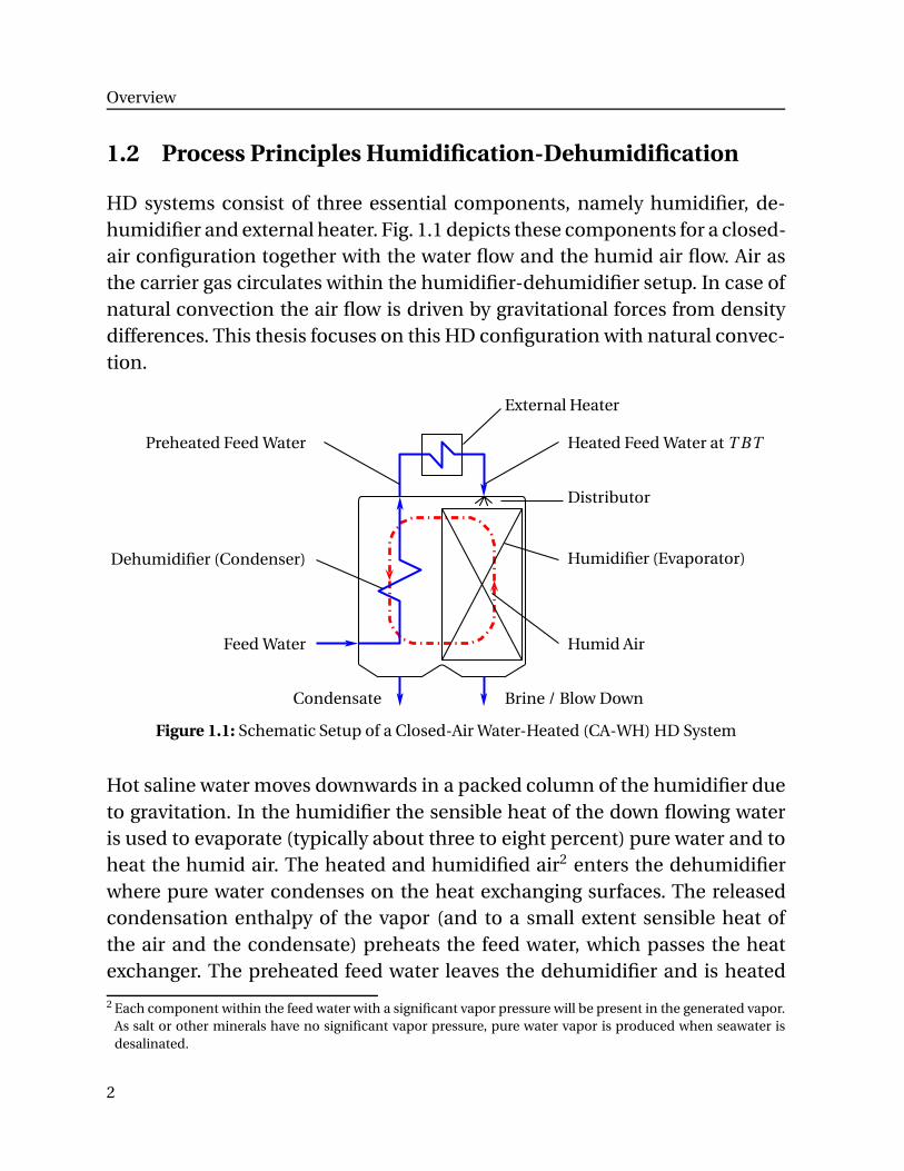
HD systems consist of three essential components, namely humidifier, de-humidifier and external heater. Fig. 1.1 depicts these components for a closed-air configuration together with the water flow and the humid air flow. Air asthe carrier gas circulates within the humidifier-dehumidifier setup. In case ofnatural convection the air flow is driven by gravitational forces from densitydifferences. This thesis focuses on this HD configuration with natural convec-tion.
Humid Air
Dehumidifier (Condenser)
Heated Feed Water at T BT
Brine / Blow Down
Feed Water
Preheated Feed Water
Condensate
External Heater
Humidifier (Evaporator)
Distributor
Figure 1.1: Schematic Setup of a Closed-Air Water-Heated (CA-WH) HD System
Hot saline water moves downwards in a packed column of the humidifier dueto gravitation. In the humidifier the sensible heat of the down flowing wateris used to evaporate (typically about three to eight percent) pure water and toheat the humid air. The heated and humidified air2 enters the dehumidifierwhere pure water condenses on the heat exchanging surfaces. The releasedcondensation enthalpy of the vapor (and to a small extent sensible heat ofthe air and the condensate) preheats the feed water, which passes the heatexchanger. The preheated feed water leaves the dehumidifier and is heated
2 Each component within the feed water with a significant vapor pressure will be present in the generated vapor.As salt or other minerals have no significant vapor pressure, pure water vapor is produced when seawater isdesalinated.
2
1.2 Process Principles Humidification-Dehumidification
further in the external heater to the top brine temperature (T BT ). The heatedwater is spread onto the packed column of the humidifier whilst the cooledand dehumidified air from the dehumidifier enters the humidifier. For naturalconvection, the air flow is driven by the density difference resulting from tem-perature and humidity differences. In forced convection systems, the air flowis enhanced by mechanical ventilation.
For steady-state conditions, i.e. conditions not depending on time, the con-densate flow MCond is a function of the constant mass flow G of dry air and thedifference in absolute humidity X = MW/MG of the air at the air inlet (top) andoutlet (bottom) of the dehumidifier:
MCond = G · (X in−Xout) . (1.1)
The partial pressure pV,sat of water vapor in saturated air and the correspond-ing absolute humidity Xsat of saturated humid air at temperature t at totalpressure p increase significantly with increasing temperature [3, p. 292]:
Xsat(t , p) =MV,sat
MG=
RG
RW·
pV,sat(t )
p −pV,sat(t ). (1.2)
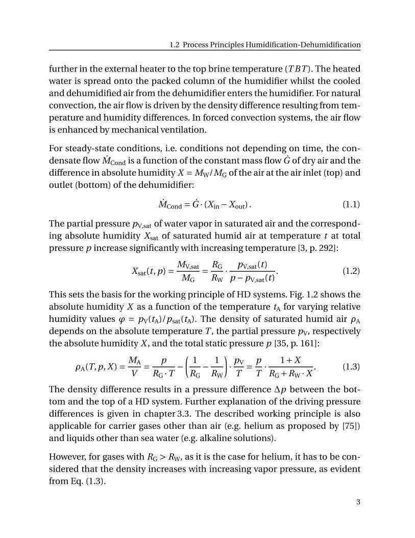
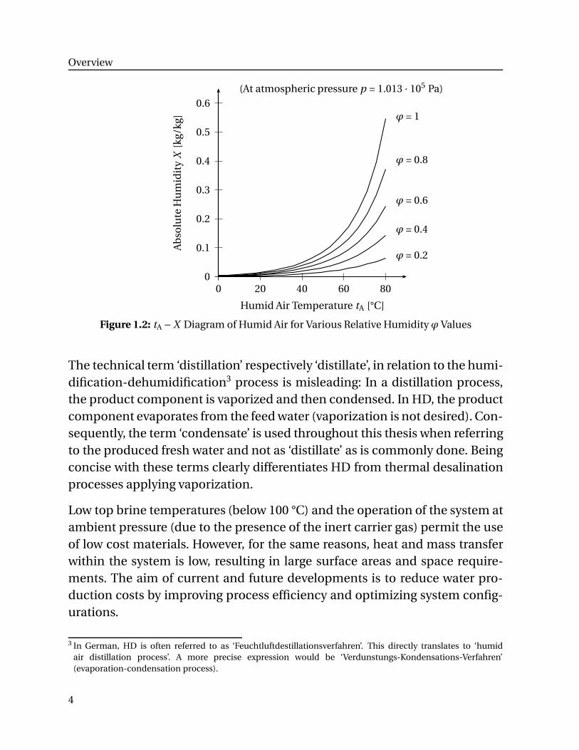
This sets the basis for the working principle of HD systems. Fig. 1.2 shows theabsolute humidity X as a function of the temperature tA for varying relativehumidity values ϕ = pV(tA)/psat(tA). The density of saturated humid air ρA
depends on the absolute temperature T , the partial pressure pV, respectivelythe absolute humidity X , and the total static pressure p [35, p. 161]:
ρA(T, p, X ) =MA
V=
p
RG ·T−
(1
RG−
1
RW
)
·pV
T=
p
T·
1+X
RG+RW · X. (1.3)
The density difference results in a pressure difference ∆p between the bot-tom and the top of a HD system. Further explanation of the driving pressuredifferences is given in chapter 3.3. The described working principle is alsoapplicable for carrier gases other than air (e.g. helium as proposed by [75])and liquids other than sea water (e.g. alkaline solutions).
However, for gases with RG > RW, as it is the case for helium, it has to be con-sidered that the density increases with increasing vapor pressure, as evidentfrom Eq. (1.3).
3
Overview
0
0.1
0.2
0.3
0.4
0.5
0.6
0 20 40 60 80
Humid Air Temperature tA [°C]
Ab
solu
teH
um
idit
yX
[kg/
kg] ϕ = 1
ϕ = 0.8
ϕ = 0.6
ϕ = 0.4
ϕ = 0.2
(At atmospheric pressure p = 1.013 · 105 Pa)
Figure 1.2: tA −X Diagram of Humid Air for Various Relative Humidity ϕ Values
The technical term ‘distillation’ respectively ‘distillate’, in relation to the humi-dification-dehumidification3 process is misleading: In a distillation process,the product component is vaporized and then condensed. In HD, the productcomponent evaporates from the feed water (vaporization is not desired). Con-sequently, the term ‘condensate’ is used throughout this thesis when referringto the produced fresh water and not as ‘distillate’ as is commonly done. Beingconcise with these terms clearly differentiates HD from thermal desalinationprocesses applying vaporization.
Low top brine temperatures (below 100 °C) and the operation of the system atambient pressure (due to the presence of the inert carrier gas) permit the useof low cost materials. However, for the same reasons, heat and mass transferwithin the system is low, resulting in large surface areas and space require-ments. The aim of current and future developments is to reduce water pro-duction costs by improving process efficiency and optimizing system config-urations.
3 In German, HD is often referred to as ‘Feuchtluftdestillationsverfahren’. This directly translates to ‘humidair distillation process’. A more precise expression would be ‘Verdunstungs-Kondensations-Verfahren’(evaporation-condensation process).
4
1.3 Objectives and Outline
1.3 Objectives and Outline
The scope of this work is to analyse a closed-air water-heated HD systemwith natural convection using experimental and analytical investigations andto contribute towards the identification of its performance limitations. Thefollowing overview outlines the key findings of each chapter.
Chapter 1 introduces HD and describes the fundamental working principleand terminology of this technology. It appears that the condensation massflow rate in HD systems with natural convection could be increased byincreasing the mean humid air temperature within the dehumidifier.
Chapter 2 proposes an extended classification of HD technologies andrelevant literature. Generally, low performance ratios are reported for systemswith natural convection. Several improvement configurations proposed inthe literature are mentioned. A common objective of these improvementsis to adjust the ratio of feed water flow rate and air flow rate. For naturalconvection setups, this can be achieved with a multi-stage configuration,whereby the total humidifier and dehumidifier column height is segmentedinto several smaller systems. This method is further investigated in this work.
Chapter 3 describes the humidification and dehumidification processes andbasic principles of natural convection. A focus is set on the physical character-istics within HD, such as uni-directional mass transfer. The dehumidificationprocess covers indirect condensation in the presence of a carrier gas and thebasics of film and dropwise condensation. Film condensation is commonlyused to describe the dehumidification process in HD. Dropwise condensationis unexpectedly observed in the experiments; however, the very high heattransfer coefficients reported in literature cannot be achieved in HD due tothe presence of non-condensable gases.
Chapter 4 summarizes the mathematical principles of the humidification anddehumidification process required for the 1-D numerical model. These rela-tions are also essential to visualize heat and mass transfer, which are usedto investigate the limitations of configurations with natural convection. Thecalculation of the interface temperature between humid air and water is of
5
Overview
special interest as it is a determining factor of the driving potential for heatand mass transfer.
Chapter 5 describes the experimental setups of the closed-air water-heatedHD configurations. The experimental configurations were adapted andcontinuously improved over time. This included several single-stage andtwo-stage setups. Investigations were undertaken in the laboratory andadditionally in two field tests in Greece and Dubai using solar collectors. Theyproved that the chosen control strategy results in an adequate performance.The developed and tested control method for the water flow is described.The advantages for transient heat input are presented, which is of particularinterest for solar powered systems. The experimental investigations of thedehumidification process of humid air showed that dropwise condensationcontinuously occurs on the plastic heat exchanger. A simplified approach forthe highly complex dropwise condensation process was established for HD todescribe the condensation process in the presence of non-condensable gases.
Chapter 6 analyses the results from the experimental and numerical in-vestigations. Since literature demonstrates no consensus about a favouredoptimization figure [30, 71, 93], an adapted performance ratio P RHD isintroduced which takes into account temperature differences. The efficiencyof a HD system is determined more accurately compared to the methodsusually applied for HD wherein condensate mass flow rates are needed, whichhave potentially significant measurement errors for small-scale systems. Theinfluence of increased water inlet temperature on both single- and two-stageHD configuration with natural convection is investigated. Through combiningexperimental data with numerical simulation and visualizing heat and masstransfer relations it is possible to identify the limitations of natural convectionsetups and describe influential factors.
Chapter 7 concludes that the HD system with natural convection has anadvantageous system setup, but lacks an inherent ability to significantlyincrease the performance ratio. The described efforts to increase the per-formance show unsatisfactory results. This becomes apparent as soon as themore precise performance ratio P RHD is applied. Based on these findings,measures to improve the performance of HD are recommended.
6
2 Literature Overview
This chapter proposes a HD classification and gives an overview of selectedliterature which is structured according to the classification.
2.1 System Classifications
HD systems configurations are usually classified by both air and water flow,whereby closed-air open-water (CAOW) and closed-water open-air (CWOA)configurations are commonly distinguished. Narayan [80] classified HD sys-tems in three categories: energy source (e.g. solar or geothermal), cycle con-figuration (closed-water open-air and closed-air, both with natural or forcedconvection) and type of heating used (water and/or air heating).
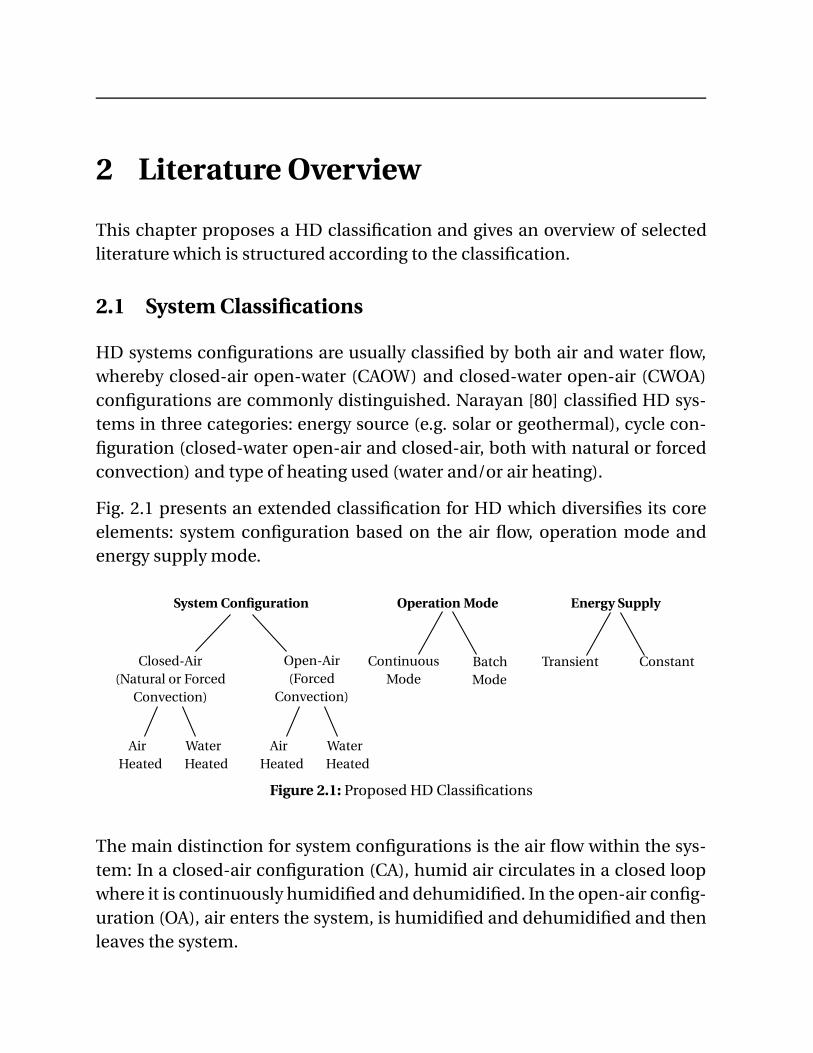
Fig. 2.1 presents an extended classification for HD which diversifies its coreelements: system configuration based on the air flow, operation mode andenergy supply mode.
System Configuration
Closed-Air(Natural or Forced
Convection)
AirHeated
WaterHeated
Open-Air(Forced
Convection)
AirHeated
WaterHeated
Operation Mode
ContinuousMode
BatchMode
Energy Supply
Transient Constant
Figure 2.1: Proposed HD Classifications
The main distinction for system configurations is the air flow within the sys-tem: In a closed-air configuration (CA), humid air circulates in a closed loopwhere it is continuously humidified and dehumidified. In the open-air config-uration (OA), air enters the system, is humidified and dehumidified and thenleaves the system.
Literature Overview
2.2 System Configurations
2.2.1 Closed-Air HD
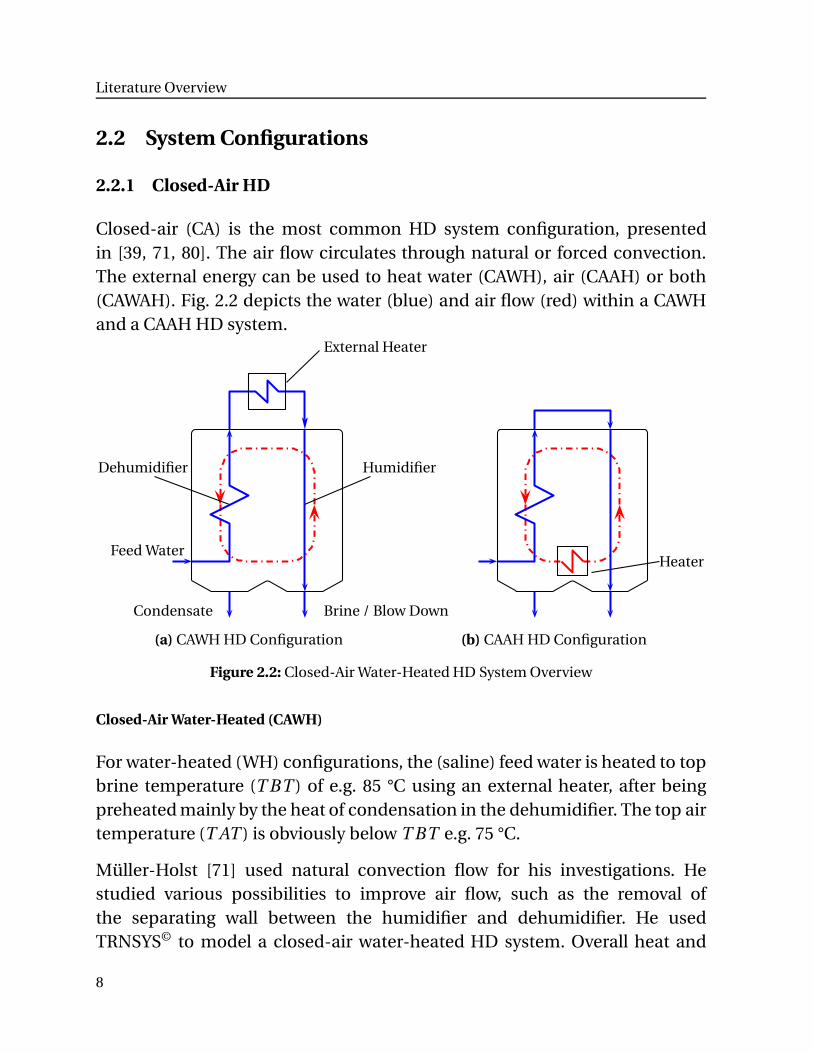
Closed-air (CA) is the most common HD system configuration, presentedin [39, 71, 80]. The air flow circulates through natural or forced convection.The external energy can be used to heat water (CAWH), air (CAAH) or both(CAWAH). Fig. 2.2 depicts the water (blue) and air flow (red) within a CAWHand a CAAH HD system.
Dehumidifier Humidifier
Brine / Blow Down
Feed Water
Condensate
External Heater
(a) CAWH HD Configuration
Heater
(b) CAAH HD Configuration
Figure 2.2: Closed-Air Water-Heated HD System Overview
Closed-Air Water-Heated (CAWH)
For water-heated (WH) configurations, the (saline) feed water is heated to topbrine temperature (T BT ) of e.g. 85 °C using an external heater, after beingpreheated mainly by the heat of condensation in the dehumidifier. The top airtemperature (T AT ) is obviously below T BT e.g. 75 °C.
Müller-Holst [71] used natural convection flow for his investigations. Hestudied various possibilities to improve air flow, such as the removal ofthe separating wall between the humidifier and dehumidifier. He usedTRNSYS© to model a closed-air water-heated HD system. Overall heat and
8
2.2 System Configurations
mass transfer equations were developed and validated with experimentsfor the characteristic water and air flow in a fleece humidifier and a flatplate dehumidifier. From the resulting data, an overall transfer coefficientwas introduced which accounts for the heat transfer from the water in thehumidifier to the water flowing in the dehumidifier. This simplification formsthe basis for the numerical simulation tool.
Nawayseh et al. [83] described a simulation model with several simplificationsto determine potentials for optimizations. They compared the results withexperimental investigations from a closed-air water-heated HD configura-tion with natural and forced convection, described in [28]. In a subsequentpublication [81], they used empirical heat and mass transfer correlations [39]and adjusted by correlations derived from experimental investigations.
Nawayseh and Farid [29, 82] used the previous findings to develop a simu-lation tool to investigate the influence of several parameters. They tested aclosed-air HD unit with natural and forced convection and developed a cal-culation program to determine the performance of the desalination unit. Theeffect between the difference of air flow rate for natural or forced convectionwas found to be negligible. Investigations with constant energy input andconstant air mass flow showed that increased feed water flow rates loweredthe operating temperature in the solar collectors resulting in higher collec-tor efficiencies but lower evaporation rates. Their model uses six equationsderived from mass balances for the humidifier and dehumidifier and the ex-ternal heater as well as equations for the heat and mass transfer, wherebylogarithmic temperature and concentration differences are applied. Accord-ing to the study, natural convection is preferred over forced convection. Thisconclusion is further investigated in chapter 4.5.2.
Al-Hallay [39] and Farid [28] continued the experimentation of Nawayseh [83]on natural and forced convection. They state that forced convection is optimalfor low top brine temperatures (up to 50 °C) whereas a small performance in-crease was determined for natural convection for higher temperatures (70 °Cand more). In a field test, two units were studied in Jordan and Malaysia [81].A new design for the system in Malaysia included larger contact areas of bothhumidifier and dehumidifier, improving the productivity of the unit. It is men-
9
Literature Overview
tioned that the effect of the air flow rate on the production rate is small. Forthis case it was concluded from experiments and numerical simulation thatthe water flow rate has greater influence on heat and mass transfer than theair flow rate.
In chapter 6 of this work, the influence of the mass flow ratios of water andair are analysed in detail. A HD system operated in forced convection canbe equipped with a humidifier and dehumidifier with higher specific surfaceareas to compensate the pressure drop. As this is not possible in setups withnatural convection, comparisons of natural and forced convection systemsshould acknowledge the different heat transfer areas.
Narayan et al. [79] studied the overall energy and mass balances for thehumidifier, the dehumidifier and the external heater along with estimatedcomponent effectiveness and relative humidity at the exit of each component.Several plant configurations were numerically studied with an assumedeffectiveness for humidifier and dehumidifier. Numerous parameter studiesdemonstrated the influence of selected parameters on the plant performance.Parameter studies are limited to the investigation of only few variable pa-rameters and a larger number of constant parameters at a time. Since theeffectiveness of each component is strongly dependent on the operationconditions and operating transfer potentials, parameter studies have notbeen pursued for this work.
Soufari et al. [93] modeled a HD process using governing equations with sev-eral simplifications gaining a heat balance for the interface between water andair for the humidifier and dehumidifier. It was identified that the water to airmass flow ratio for a setup with forced convection reaches an optimum. Thereasons for this behaviour for single-stage systems are investigated in chapters6 and 7. The recycling of brine from the humidifier into the feed water of thedehumidifier is described as a method to reduce specific energy consumption.
Bacha et al. [1] modeled the heat and mass transfer equations for steady-stateoperation. Investigations for solar powered HD systems followed [2] wherebyhot water is produced and stored during times with high solar irradiationto be used during night time. This concept has also been described by [46].
10
2.2 System Configurations
This method which aims to increase the total water output per day dependson the available solar collector area and heat storage capacity. It avoids thedisadvantages of the transient phases during heat up. This effect is discussedin subsection 5.3.2.
Hou et al. [49] investigated the pinch point method to optimize a HD systemwith constant ratio between the water L and air G mass flow rate. As the pinchpoint method aims to minimise the driving temperature difference betweenwater and saturated air, the required products of transfer surfaces and coeffi-cients become very large. It is shown that even for this case, the ratio betweenthe recovered enthalpy flow and the (externally) added heat flow is limited tosmall values. The described method is not suitable to describe a system forwhich the ratio L/G can be adjusted along the column height.
Hassabou [40] established a 1-D simulation model. The governing equationswere solved with Matlab©. The impact of the heat conductivity on the humidi-fier and dehumidifier for closed-air water-heated configuration with forcedconvection and direct heat exchange in the dehumidifier was simulated.
Various works are reported on water heated systems with T BT in the rangebetween 50 °C and 90 °C. From 50 °C to 70 °C e.g. by [39], 60 °C e.g. [58],between 70 °C and 80 °C e.g. by [81] or from 80 °C to 90 °C e.g. by [72]. Theeffect on the mass transfer for low operating top brine temperatures (35 °Cand 45 °C) was investigated [25].
Closed-Air Air-Heated (CAAH)
Dehumidified air is heated with an external heater before entering thehumidifier, see Fig. 2.2 (b). This process can be repeated in multiple stages,as suggested e.g. by Chafik et al. [12]. Heating air instead of feed watersignificantly reduces the scale formation and corrosion potential. The smallheat transfer coefficient in the air-heater and the low heat capacity of air aredisadvantageous, resulting in low condensate water production and largeheat exchanger surfaces.
11
Literature Overview
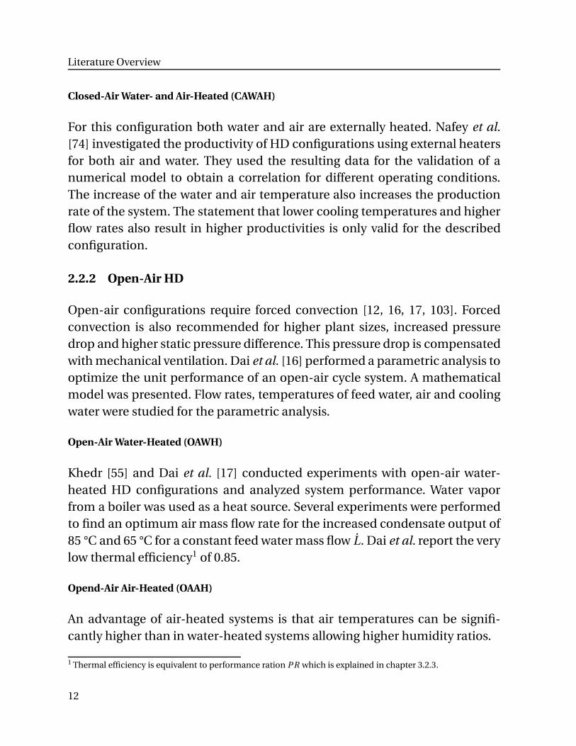
Closed-Air Water- and Air-Heated (CAWAH)
For this configuration both water and air are externally heated. Nafey et al.[74] investigated the productivity of HD configurations using external heatersfor both air and water. They used the resulting data for the validation of anumerical model to obtain a correlation for different operating conditions.The increase of the water and air temperature also increases the productionrate of the system. The statement that lower cooling temperatures and higherflow rates also result in higher productivities is only valid for the describedconfiguration.
2.2.2 Open-Air HD
Open-air configurations require forced convection [12, 16, 17, 103]. Forcedconvection is also recommended for higher plant sizes, increased pressuredrop and higher static pressure difference. This pressure drop is compensatedwith mechanical ventilation. Dai et al. [16] performed a parametric analysis tooptimize the unit performance of an open-air cycle system. A mathematicalmodel was presented. Flow rates, temperatures of feed water, air and coolingwater were studied for the parametric analysis.
Open-Air Water-Heated (OAWH)
Khedr [55] and Dai et al. [17] conducted experiments with open-air water-heated HD configurations and analyzed system performance. Water vaporfrom a boiler was used as a heat source. Several experiments were performedto find an optimum air mass flow rate for the increased condensate output of85 °C and 65 °C for a constant feed water mass flow L. Dai et al. report the verylow thermal efficiency1 of 0.85.
Opend-Air Air-Heated (OAAH)
An advantage of air-heated systems is that air temperatures can be signifi-cantly higher than in water-heated systems allowing higher humidity ratios.
1 Thermal efficiency is equivalent to performance ration PR which is explained in chapter 3.2.3.
12
2.3 Operation Modes
Kolb [60] states that using solar air collectors with a air inlet temperature of30 °C, an outlet temperature of 80 °C can only be achieved for air mass flowdensities as low as 0.01 kg/(m2·s). Due to heat loss, the efficiency for solar flatplate collectors decreases with higher operation temperatures. The efficiencyof the collector can be as low as 20% for such high air temperatures.
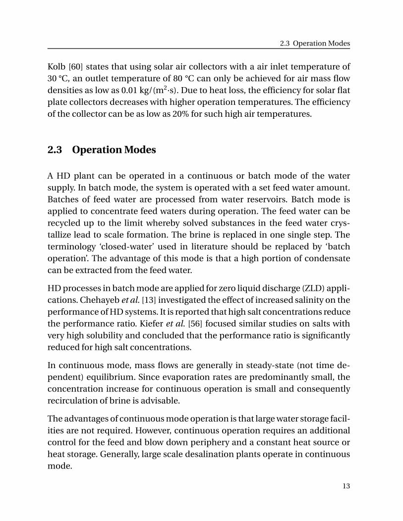
2.3 Operation Modes
A HD plant can be operated in a continuous or batch mode of the watersupply. In batch mode, the system is operated with a set feed water amount.Batches of feed water are processed from water reservoirs. Batch mode isapplied to concentrate feed waters during operation. The feed water can berecycled up to the limit whereby solved substances in the feed water crys-tallize lead to scale formation. The brine is replaced in one single step. Theterminology ‘closed-water’ used in literature should be replaced by ‘batchoperation’. The advantage of this mode is that a high portion of condensatecan be extracted from the feed water.
HD processes in batch mode are applied for zero liquid discharge (ZLD) appli-cations. Chehayeb et al. [13] investigated the effect of increased salinity on theperformance of HD systems. It is reported that high salt concentrations reducethe performance ratio. Kiefer et al. [56] focused similar studies on salts withvery high solubility and concluded that the performance ratio is significantlyreduced for high salt concentrations.
In continuous mode, mass flows are generally in steady-state (not time de-pendent) equilibrium. Since evaporation rates are predominantly small, theconcentration increase for continuous operation is small and consequentlyrecirculation of brine is advisable.
The advantages of continuous mode operation is that large water storage facil-ities are not required. However, continuous operation requires an additionalcontrol for the feed and blow down periphery and a constant heat source orheat storage. Generally, large scale desalination plants operate in continuousmode.
13
Literature Overview
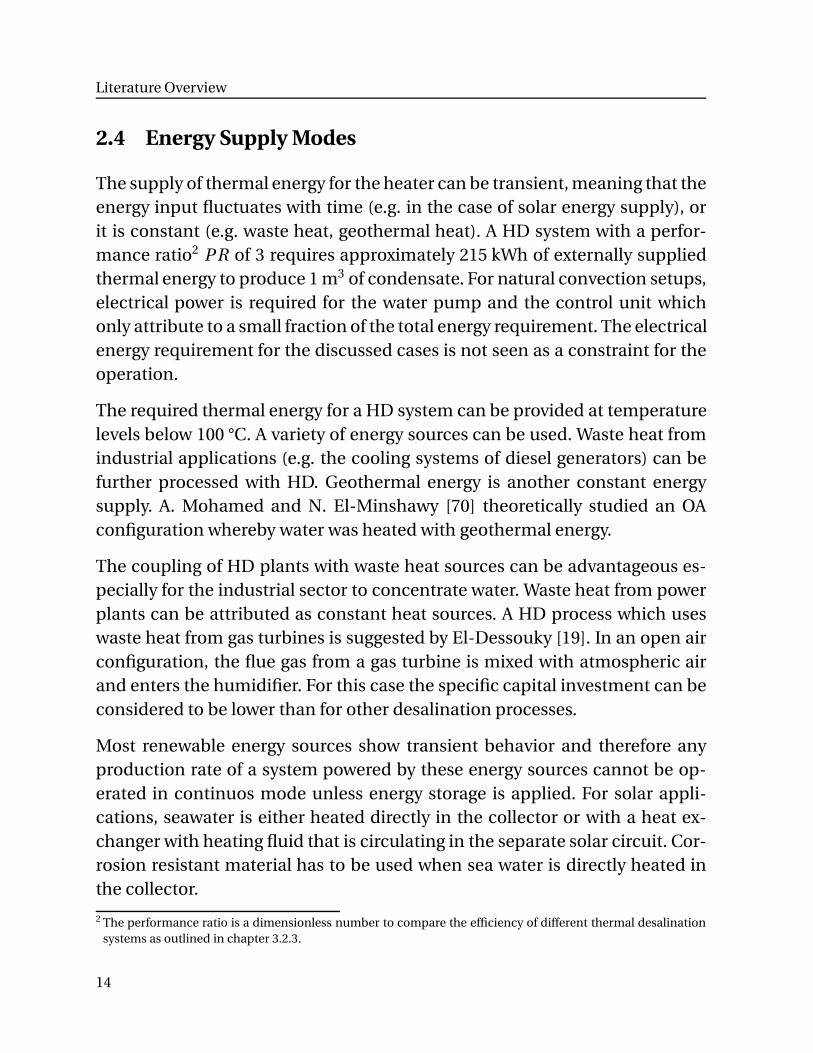
2.4 Energy Supply Modes
The supply of thermal energy for the heater can be transient, meaning that theenergy input fluctuates with time (e.g. in the case of solar energy supply), orit is constant (e.g. waste heat, geothermal heat). A HD system with a perfor-mance ratio2 P R of 3 requires approximately 215 kWh of externally suppliedthermal energy to produce 1 m3 of condensate. For natural convection setups,electrical power is required for the water pump and the control unit whichonly attribute to a small fraction of the total energy requirement. The electricalenergy requirement for the discussed cases is not seen as a constraint for theoperation.
The required thermal energy for a HD system can be provided at temperaturelevels below 100 °C. A variety of energy sources can be used. Waste heat fromindustrial applications (e.g. the cooling systems of diesel generators) can befurther processed with HD. Geothermal energy is another constant energysupply. A. Mohamed and N. El-Minshawy [70] theoretically studied an OAconfiguration whereby water was heated with geothermal energy.
The coupling of HD plants with waste heat sources can be advantageous es-pecially for the industrial sector to concentrate water. Waste heat from powerplants can be attributed as constant heat sources. A HD process which useswaste heat from gas turbines is suggested by El-Dessouky [19]. In an open airconfiguration, the flue gas from a gas turbine is mixed with atmospheric airand enters the humidifier. For this case the specific capital investment can beconsidered to be lower than for other desalination processes.
Most renewable energy sources show transient behavior and therefore anyproduction rate of a system powered by these energy sources cannot be op-erated in continuos mode unless energy storage is applied. For solar appli-cations, seawater is either heated directly in the collector or with a heat ex-changer with heating fluid that is circulating in the separate solar circuit. Cor-rosion resistant material has to be used when sea water is directly heated inthe collector.
2 The performance ratio is a dimensionless number to compare the efficiency of different thermal desalinationsystems as outlined in chapter 3.2.3.
14
2.5 Improved Configurations
When heat exchangers are used, additional thermal losses need to be consid-ered along with additional technical efforts including plant control. Several re-search institutes developed systems for an efficient use of water desalinationusing solar energy [12, 16, 39, 43, 94, 96]. A reservoir of heated brine comingfrom the collector supports the continuous operation of the desalination plantduring times without solar radiation [71]. This of course requires a larger col-lector area and an additional hot water storage capacity.
Rodriguez et al. [31] and Tzen et al. [98] provided a general overview ofdesalination systems powered by renewable energy, both of large and smallscale. Parekh et al. [84] focused on system configurations using solar energyand outlined a detailed technical overview of existing systems.
Early investigations and tests using plastics for flat plate collectors startedbefore 1978 [85]. Technical developments are described in [42, 87] for seawaterapplications. Flat plate collectors are mostly used for domestic water heatingto temperatures of up to 60 °C. Thermal losses significantly increase withhigher water outlet temperatures [23, p. 302]. Selective absorber material re-duces thermal losses [53]. Evacuated tube collectors (heat pipes) reach higheroperation temperatures and have, compared to flat plate collectors, signifi-cantly smaller heat losses [52, p. 131].
2.5 Improved Configurations
To increase the efficiency of HD systems, several improvements have beensuggested in literature, in particular air extraction, water extraction and multi-staging.
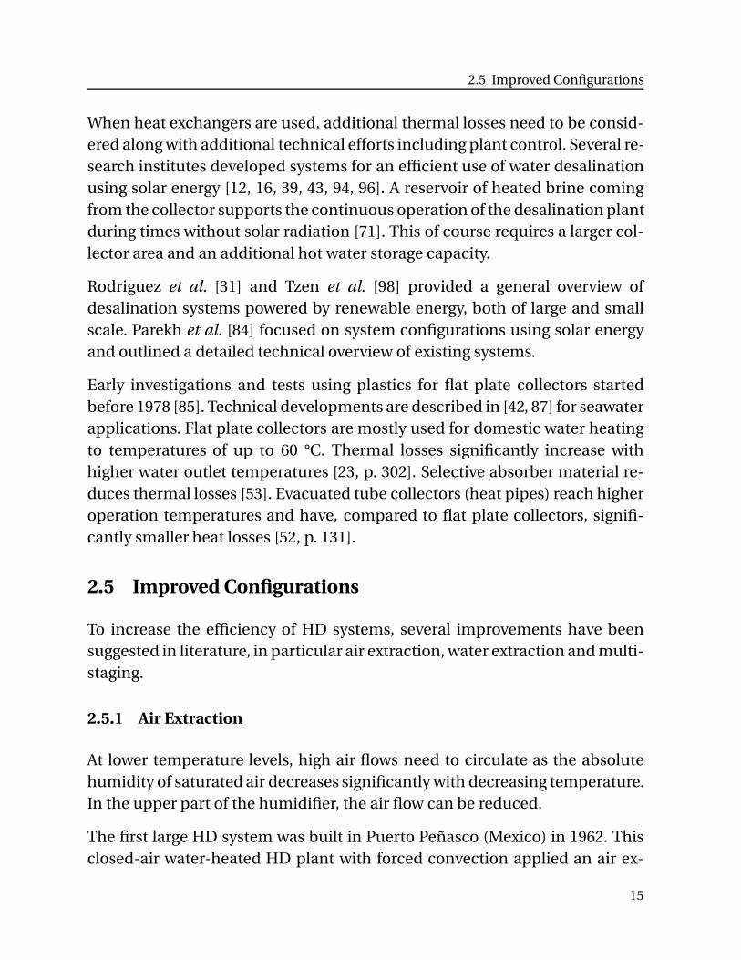
2.5.1 Air Extraction
At lower temperature levels, high air flows need to circulate as the absolutehumidity of saturated air decreases significantly with decreasing temperature.In the upper part of the humidifier, the air flow can be reduced.
The first large HD system was built in Puerto Peñasco (Mexico) in 1962. Thisclosed-air water-heated HD plant with forced convection applied an air ex-
15
Literature Overview
traction setup [47, 90]. Hodges et. al called these air extraction flows ‘bleed-offs’ [45]. By adjusting the air flows, the slope of the operating line3 is adjustedto the slope of the saturation line4. Air extraction is favourably applied inforced convection system configurations.
Müller-Holst [71] claims that by removing the separation wall betweenhumidifier and dehumidifier the air mass flow is positively adjusted whichmeans that the mass flow is higher at the lower part of the system comparedto the upper part. He supposes that this is an automatically optimizing system.
2.5.2 Water Extraction
Instead of increasing the air mass flow in the lower part of the column, theslope of the operating line can be optimzed through extracting water fromthe humidifier to recirculate it to the dehumidifier, as depicted in Fig. 5.1(b). Brendel [9, 10] investigated the effects of the different heat capacity flowsof water and air and suggests that instead of air flow, the water flow can beadjusted. At certain heights, a certain ratio of water flow from the dehumidifieris extracted and injected in the humidifier at the corresponding height.
Another way to recover heat is by injecting brine leaving the dehumidifierinto the feed water entering the humidifier. This leads to an overall elevatedtemperature level of the system whereby for a given external energy input themass flow rate can be increased. This is investigated in the presented work.
2.5.3 Multi-Staging
The concept of multi-staging is applied in conventional thermal desalinationsystems such as multi-stage flash (MSF) or multi-effect distillation (MED).The produced vapor from one stage flows to the subsequent stage where itis used to either preheat or vaporize feed water. Water vaporizes in each stageresulting in lower water temperatures in the subsequent stages. The individualstages in MSF and MED plants are operated at consecutively reduced pressure
3 The operating line is a graphic indicator applied for the humidifier and dehumidifier to determine optimizedwater and air flow ratios. For the humidifier, cp. chapter 4.3.3 and for the dehumidifier, cp. chapter 4.4.1.
4 The saturation line indicates the specific enthalpy of saturated humid air for a given air temperature. Thedriving potentials for heat and mass transfer vanishes when the operating line approaches the saturation line.
16
2.5 Improved Configurations
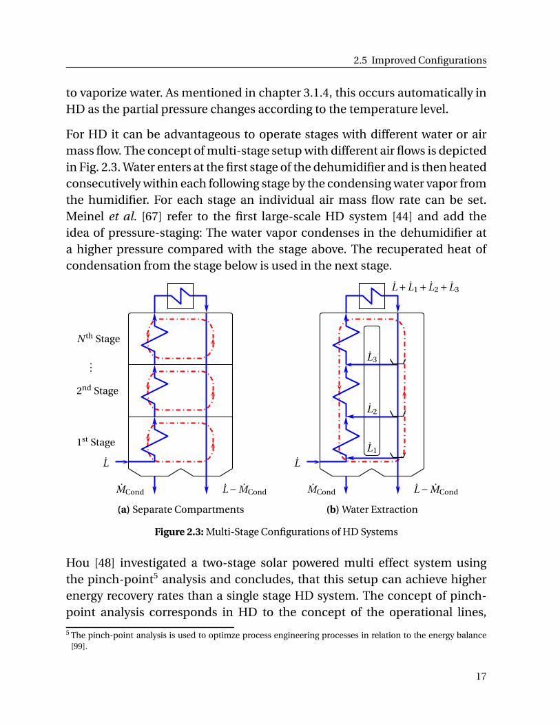
to vaporize water. As mentioned in chapter 3.1.4, this occurs automatically inHD as the partial pressure changes according to the temperature level.
For HD it can be advantageous to operate stages with different water or airmass flow. The concept of multi-stage setup with different air flows is depictedin Fig. 2.3. Water enters at the first stage of the dehumidifier and is then heatedconsecutively within each following stage by the condensing water vapor fromthe humidifier. For each stage an individual air mass flow rate can be set.Meinel et al. [67] refer to the first large-scale HD system [44] and add theidea of pressure-staging: The water vapor condenses in the dehumidifier ata higher pressure compared with the stage above. The recuperated heat ofcondensation from the stage below is used in the next stage.
1st Stage
2nd Stage
...
N th Stage
MCond L− MCond
L
(a) Separate Compartments
MCond L − MCond
L
L1
L2
L3
L + L1 + L2 + L3
(b) Water Extraction
Figure 2.3: Multi-Stage Configurations of HD Systems
Hou [48] investigated a two-stage solar powered multi effect system usingthe pinch-point5 analysis and concludes, that this setup can achieve higherenergy recovery rates than a single stage HD system. The concept of pinch-point analysis corresponds in HD to the concept of the operational lines,
5 The pinch-point analysis is used to optimze process engineering processes in relation to the energy balance[99].
17
Literature Overview
described in chapter 4.3.3. Zamen [104] worked on the improvement of solarpowered HD using a multi-stage process and operated a 500 l/d unit in Iranwhereby a 20% reduction of investment cost was reported compared to asingle stage unit with the same capacity.
For closed-air water-heated HD systems, Chafik [12] suggest a stepwise load-ing of the air to increase the absolute humidity within the air. This conceptwas also adapted by Hassabou [40] whereby the humidifier consisting of apacked bed including phase change material releases heat through the drypatches (non-wetted surface area of humidifier) during operation to gain asimilar effect.
Over the past years, several approaches have been published showing howto increase condensate output for HD systems, e.g. by [7, 49, 76, 80, 84, 93].Limited research has been conducted on the improvement of the air flowwithin HD systems, especially natural convection and advanced HD designs.
18
3 HD Processes
3.1 Humidification Process
3.1.1 Separation Process
A characteristic of the operation of HD is that only components with asignificant partial pressure are present in the gas phase. The dissolvedcomponents of sea water (the composition of standard seawater can be foundin [100]) do not have a significant vapor pressure1 [34].
Therefore, HD is a thermal separation process which can produce distilledwater from saline water, also from water with very high salt concentrations2.Salt water leaving the humidifier, the so called brine, has consequently ahigher salt concentration of dissolved substances that do not evaporate. Thedissolved ionic components are not transferred into the vapor, but in reality,sea water droplets or crystalline particles may be carried over by the gaseousflow to the dehumidifier.
Humidification of air corresponds to evaporative cooling that is used for manyindustrial applications with direct contact of water and air, such as in coolingtowers for power plants. Wernicke [102] gives a detailed description of thetheory of cooling towers. Distinct similarities between cooling towers and HDhumidifiers, such as the active part of the cooling tower (packing) correspondsto the packing volume of the humidifier, offer the opportunity to transfertheoretical and technological cooling tower solutions to HD where suitable.
To generate a large interface surface between water and air, water runsthrough a packed bed (industrial filling material) which is one of the keyelements to achieve increased heat and mass transfer in cooling towersand other evaporative cooling systems. Such highly sophisticated packing1 Eucken [27] calculated exemplarily the ratio of the concentration c of salt ions in the solution to the
concentration in the gas phase. This ratio is of many orders of magnitudes (cSolution/cGas ≈ 1070).2 In contrast, the required operating pressure of reverse osmosis (RO) desalination systems is strongly dependent
on the salinity of the water and consequently operation is limited to certain concentrations.
HD Processes
structures can be applied for humidifiers in HD systems for large exchangesurfaces per column volume.
In cooling towers, the operating temperature range is significantly lower thanin HD systems. Therefore, some simplifications applied for cooling towers, asintroduced by Merkel [68], are not valid for HD systems. However, the elabo-rated methods for designing cooling towers are helpful for understanding thehumidification processes and potential optimization approaches.
3.1.2 Partial Pressure and Concentration Differences
As the operating pressure in HD is low, the humid air can be considered as amixture of ideal gases3. A partial pressure difference of vapor occurs duringthe evaporation process between the vapor pressure at the water-air interfaceand the vapor pressure in the bulk flow of humid air, as further explained inchapter 4.3. The corresponding concentration difference is the driving forcefor the transport of vapor into the air bulk flow. A commonly used definitionof concentration ci of a component in gases corresponds to a molar partialdensity ρi. For a component i (index i) of an ideal gas, the partial density ρi isρi = pi/(Ri ·T ). The molar partial density ρi is calculated with the universal gasconstant R instead of the specific gas constant Ri = R/Mi. The total pressure pof humid air is the sum of the partial pressure pV of water vapor (index V) andpartial pressure pG of dry air (index G) according to Dalton’s law [88, p. 52].
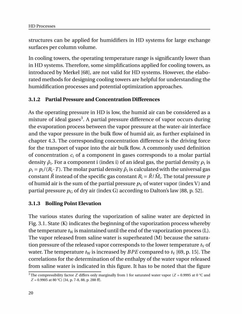
3.1.3 Boiling Point Elevation
The various states during the vaporization of saline water are depicted inFig. 3.1. State (K) indicates the beginning of the vaporization process wherebythe temperature tW is maintained until the end of the vaporization process (L).The vapor released from saline water is superheated (M) because the satura-tion pressure of the released vapor corresponds to the lower temperature tV ofwater. The temperature tW is increased by BPE compared to tV [69, p. 15]. Thecorrelations for the determination of the enthalpy of the water vapor releasedfrom saline water is indicated in this figure. It has to be noted that the figure3 The compressibility factor Z differs only marginally from 1 for saturated water vapor (Z = 0.9995 at 0 °C and
Z = 0.9905 at 80 °C) [34, p. 7-8, 88, p. 288 ff].
20
3.1 Humidification Process
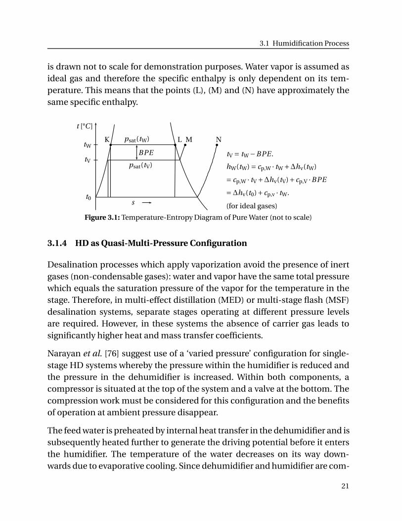
is drawn not to scale for demonstration purposes. Water vapor is assumed asideal gas and therefore the specific enthalpy is only dependent on its tem-perature. This means that the points (L), (M) and (N) have approximately thesame specific enthalpy.
t [°C ]
s
tW
tV
t0
BPE
psat(tW)
psat(tV)
K L M N
tV = tW −BPE .
hW(tW) = cp,W · tW +∆hv(tW)
= cp,W · tV +∆hv(tV)+cp,V ·BPE
=∆hv(t0)+cp,v · tW.
(for ideal gases)
Figure 3.1: Temperature-Entropy Diagram of Pure Water (not to scale)
3.1.4 HD as Quasi-Multi-Pressure Configuration
Desalination processes which apply vaporization avoid the presence of inertgases (non-condensable gases): water and vapor have the same total pressurewhich equals the saturation pressure of the vapor for the temperature in thestage. Therefore, in multi-effect distillation (MED) or multi-stage flash (MSF)desalination systems, separate stages operating at different pressure levelsare required. However, in these systems the absence of carrier gas leads tosignificantly higher heat and mass transfer coefficients.
Narayan et al. [76] suggest use of a ‘varied pressure’ configuration for single-stage HD systems whereby the pressure within the humidifier is reduced andthe pressure in the dehumidifier is increased. Within both components, acompressor is situated at the top of the system and a valve at the bottom. Thecompression work must be considered for this configuration and the benefitsof operation at ambient pressure disappear.
The feed water is preheated by internal heat transfer in the dehumidifier and issubsequently heated further to generate the driving potential before it entersthe humidifier. The temperature of the water decreases on its way down-wards due to evaporative cooling. Since dehumidifier and humidifier are com-
21
HD Processes
bined, a larger amount of water can evaporate and condense compared to aprocess in which only the external heating is used to evaporate water (com-pare also chapter 3.2.3 for the definition of the performance ratio P R). It is aninherent characteristic of the HD process that the partial pressure pV,∞ of thevapor in the bulk air and at the interface pV,I is also reduced along with thetemperature, however the total pressure ptotal remains constant. The differ-ence to the total pressure is the partial pressure pG of dry air. This resemblesa multi-pressure configuration without the need of multiple separate stagesor vessels. Therefore it is here suggested to introduce the term quasi-multi-pressure configuration for HD systems.
3.2 Dehumidification Process
Dehumidification in HD systems with indirect condensation is characterizedby the condensation of water vapor via a solid heat exchanger surface in thepresence of non-condensable gases (NCG).
Within the dehumidifier, condensable components within the humid air, herewater vapor, precipitate on the heat exchanger surfaces. Additionally, theformed liquid condensate acts as a cooling surface. This dehumidification ofhumid air is like the previously described humidification process: a coupledheat and mass transfer phenomenon including phase change. Unidirectionalmass transfer also has to be considered.
The heat of vaporization ∆hV(t ) is released during the dehumidificationprocess forming the condensate. Condensation can occur when the coolingsurface temperature is below the saturation temperature tV,sat of the vaporwith partial pressure pV. The presence of non-condensable gases (NCG)greatly influences heat and mass transfer. In HD, a dominant process forthe dehumidification is the diffusion process in the gaseous phase4. For thecondensation process, the effect of boiling point elevation is not relevant, asonly pure water condenses in the dehumidifier.
4 Baehr and Stephan show that already for small concentrations of air, e.g. pG /p = 0.1, the heat transfer is reducedto 16 % for natural convection [4, Fig. 4.10, p. 465].
22
3.2 Dehumidification Process
3.2.1 Principles of Condensation
Condensation at cooling surfaces takes place in three steps [36, p. 284]. Firstly,vapor moves towards the cooling surface by molecular or molar transportwhereby the presence of non-condensable gases and diffusion resistance canbe high. Secondly, at the cooling surface, condensation of the water vaportakes place. In a third step, heat is removed from the interface by the coolingliquid, in this case feed water.
For a process in which pure vapor condenses (no presence of NCG), the ther-mal resistance in the gaseous phase (vapor) is usually neglected. This is alsothe case for Nusselt’s water film theory [36, p. 285 ff.]. The thermal resistanceis assumed to be only in the water film. This simplification is not valid for HDprocesses.
There are two basic principles for dehumidification: direct and indirect con-tact condensation. Both principles are applicable for HD.
Direct Condensation
With direct condensation, humid air is brought in direct contact with thecooling medium, e.g. cool pure water (liquid-liquid heat exchange). Directcondensation in humid air is essentially the reverse process of humidificationof air because in this case heat removal occurs by enthalpy increase of cold(pure) water5, whereby for humidification the heat input occurs by enthalpydecrease of the hot seawater.
The correlations from the humidification process are transferred to describeheat and mass transfer processes for the dehumidification. The heat ofcondensation is recovered in an additional heat exchanger from the waterleaving the dehumidifier [62]. A setup with one mixing water temperature canbe considered as a single-stage unit without counter-current flow. ThereforeP R is low.
Direct contact heat exchangers in HD are configured as bubble [78] or spraycolumns [18, 40, 46, 57, 62, 66]. Spray columns can be equipped with or with-5 Also materials which are immiscible with and insoluble in water have been considered [47, p. 83].
23
HD Processes
out internals, such as a packing material. Distilled water or condensate is usedas the cooling liquid and is sprayed into the hot humid air flow. The air flowcan be in cocurrent or countercurrent direction to the spray. Cocurrent flowcan avoid entrainment of fine particles in forced convection setups.
The advantage of direct condensation is that heat and mass transfer can besignificantly increased compared to indirect condensers. The disadvantageis that an external liquid-liquid heat-exchanger and additional pumps arerequired to be able to recover the heat of condensation. A multi-effect config-uration with countercurrent flow can only be achieved in a multi-stage setup.
Indirect Condensation
Indirect condensation requires a solid heat exchange surface. The conden-sation occurs on the solid surface and on the liquid which is formed on thesurface6. For HD, the dehumidifier tube walls separate the cooling liquid fromthe condensate and the humid air flow. Additionally, condensation takes placeon the adhering water surface of the condensate droplet or film. Indirect con-tact heat exchange allows compact plant design since no additional exter-nal heat exchanger is required and the control of the overall system can besimplified. Furthermore, this configuration allows a modular setup enablingpossibilities for further plant optimizations and adaptations.
Preheated feed water can be extracted at virtually any point between inlet andoutlet of the dehumidifier also enabling an advantageous multi-stage config-uration. Results from experiments can be transferred to different tube dia-meters due to the reliable scalability as the heat-transfer surfaces are clearlydefined. The temperature regions for operation are still relatively low so thatlow-cost material, such as polypropylene, can be applied. On the other hand,scaling inside the tubes needs to be considered.
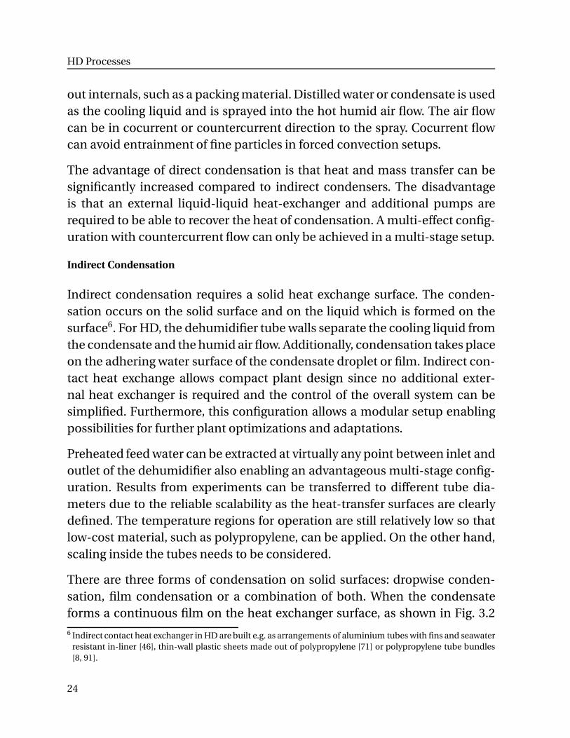
There are three forms of condensation on solid surfaces: dropwise conden-sation, film condensation or a combination of both. When the condensateforms a continuous film on the heat exchanger surface, as shown in Fig. 3.2
6 Indirect contact heat exchanger in HD are built e.g. as arrangements of aluminium tubes with fins and seawaterresistant in-liner [46], thin-wall plastic sheets made out of polypropylene [71] or polypropylene tube bundles[8, 91].
24
3.2 Dehumidification Process
(a) Film Condensation (b) Dropwise Condensation
Figure 3.2: Film and Dropwise Condensation on Tubes
(a), this phenomenon is called film condensation. The water film runs off aslaminar or turbulent flow. In the case of incomplete wetting of the exchangersurface, the condensate forms droplets on the heat exchanger surface, shownin Fig. 3.2 (b). This case is called dropwise condensation, see [4, p. 450-451].
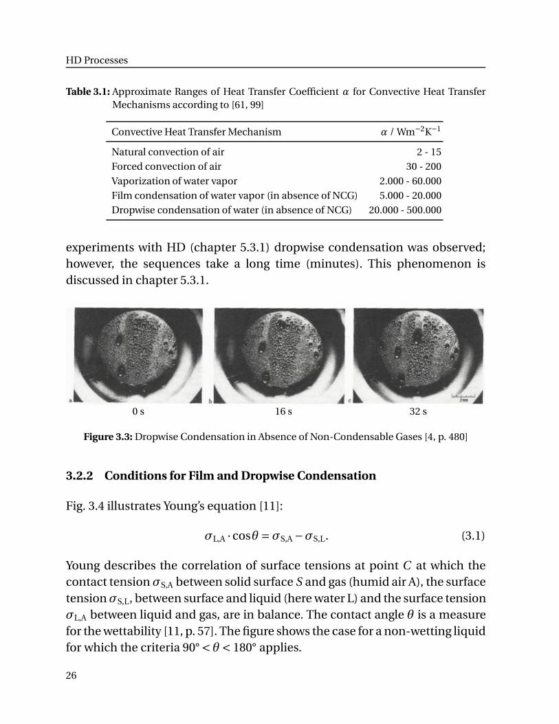
Literature usually focusses on condensation of pure vapor in the absenceof NCG [4, p. 477 ff. 33, p. 673, 36, p. 309, 61, p. 100 ff. 99, p. Ja1 ff.].Investigations on dropwise condensation started in 1930 by E. Schmidt[89]. Heat transfer with dropwise condensation in the absence of NCG canbe very high compared with other convective heat transfer mechanismsas indicated in Table 3.1. Therefore, dropwise condensation is favored inindustrial applications. Unfortunately, dropwise condensation can rarely bemaintained for a longer time period on metal surfaces without additionaltechnical efforts. These efforts include doting the vapor, coating the heatexchanger surface or ion-implementation [22, 54, 61, 86].
It has to be noted that surface conditions alter, e.g. due to corrosion effects,and due to the effect of impurities or additives. Therefore, maintaining theconditions for dropwise condensation for a long time is challenging. The va-porization and condensation rate strongly depends on the contact angle θ ofthe participating phases of the surface depicted in Fig. 3.4 [11].
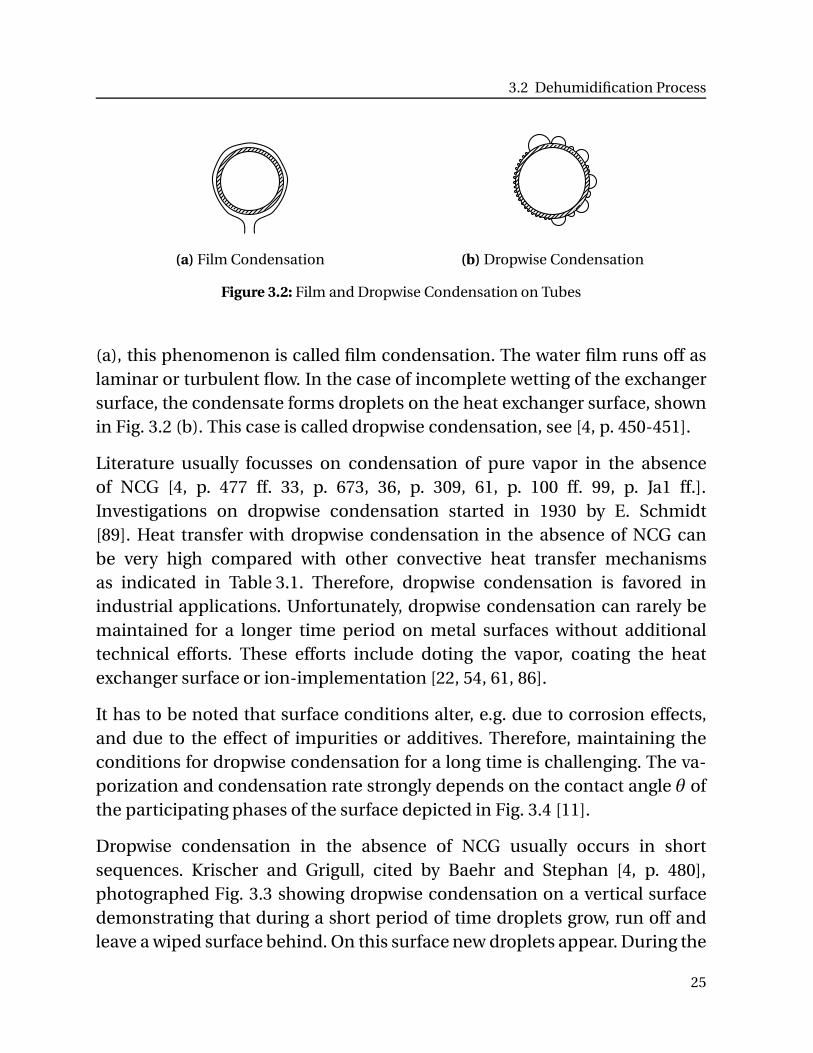
Dropwise condensation in the absence of NCG usually occurs in shortsequences. Krischer and Grigull, cited by Baehr and Stephan [4, p. 480],photographed Fig. 3.3 showing dropwise condensation on a vertical surfacedemonstrating that during a short period of time droplets grow, run off andleave a wiped surface behind. On this surface new droplets appear. During the
25
HD Processes
Table 3.1: Approximate Ranges of Heat Transfer Coefficient α for Convective Heat TransferMechanisms according to [61, 99]
Convective Heat Transfer Mechanism α / Wm−2K−1
Natural convection of air 2 - 15
Forced convection of air 30 - 200
Vaporization of water vapor 2.000 - 60.000
Film condensation of water vapor (in absence of NCG) 5.000 - 20.000
Dropwise condensation of water (in absence of NCG) 20.000 - 500.000
experiments with HD (chapter 5.3.1) dropwise condensation was observed;however, the sequences take a long time (minutes). This phenomenon isdiscussed in chapter 5.3.1.
0 s 16 s 32 s
Figure 3.3: Dropwise Condensation in Absence of Non-Condensable Gases [4, p. 480]
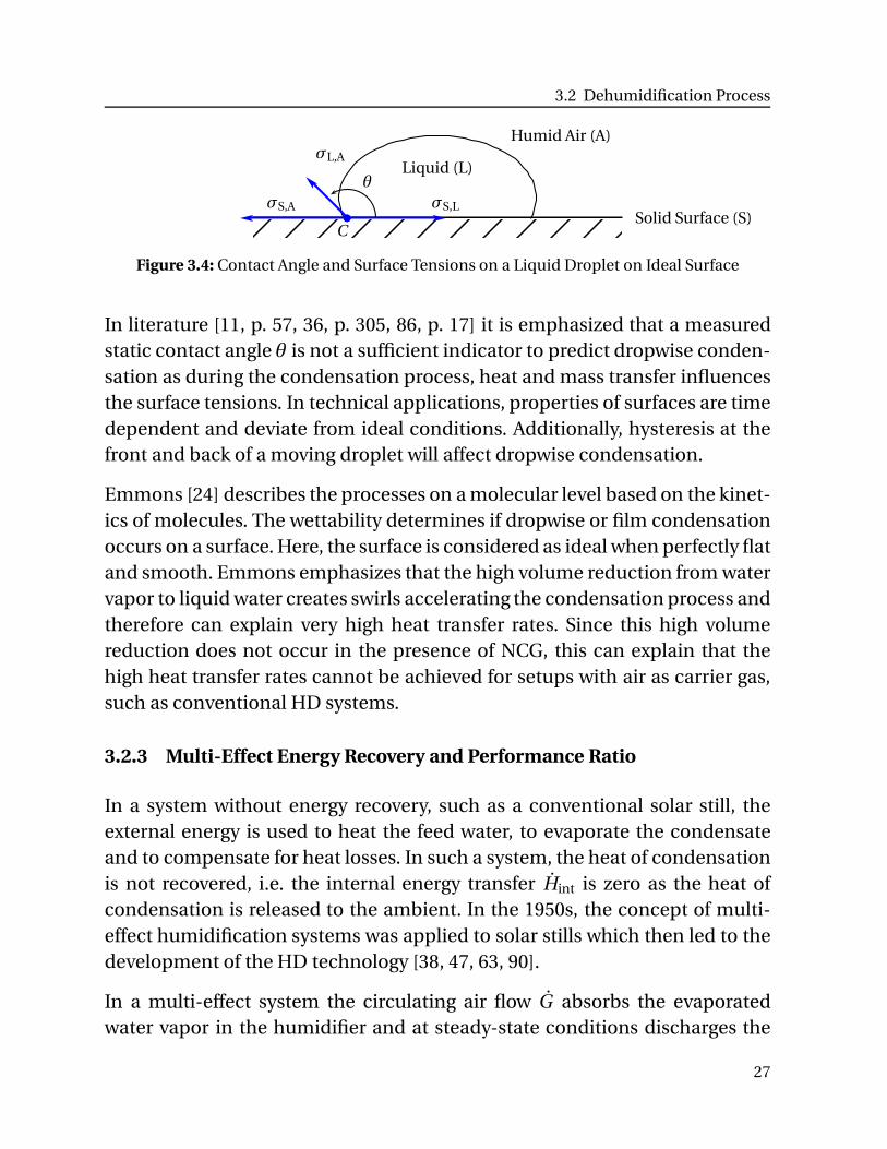
3.2.2 Conditions for Film and Dropwise Condensation
Fig. 3.4 illustrates Young’s equation [11]:
σL,A ·cosθ =σS,A −σS,L. (3.1)
Young describes the correlation of surface tensions at point C at which thecontact tension σS,A between solid surface S and gas (humid air A), the surfacetension σS,L, between surface and liquid (here water L) and the surface tensionσL,A between liquid and gas, are in balance. The contact angle θ is a measurefor the wettability [11, p. 57]. The figure shows the case for a non-wetting liquidfor which the criteria 90° < θ < 180° applies.
26
3.2 Dehumidification Process
Solid Surface (S)
Humid Air (A)
Liquid (L)
σS,A σS,L
σL,A
θ
C
Figure 3.4: Contact Angle and Surface Tensions on a Liquid Droplet on Ideal Surface
In literature [11, p. 57, 36, p. 305, 86, p. 17] it is emphasized that a measuredstatic contact angle θ is not a sufficient indicator to predict dropwise conden-sation as during the condensation process, heat and mass transfer influencesthe surface tensions. In technical applications, properties of surfaces are timedependent and deviate from ideal conditions. Additionally, hysteresis at thefront and back of a moving droplet will affect dropwise condensation.
Emmons [24] describes the processes on a molecular level based on the kinet-ics of molecules. The wettability determines if dropwise or film condensationoccurs on a surface. Here, the surface is considered as ideal when perfectly flatand smooth. Emmons emphasizes that the high volume reduction from watervapor to liquid water creates swirls accelerating the condensation process andtherefore can explain very high heat transfer rates. Since this high volumereduction does not occur in the presence of NCG, this can explain that thehigh heat transfer rates cannot be achieved for setups with air as carrier gas,such as conventional HD systems.
3.2.3 Multi-Effect Energy Recovery and Performance Ratio
In a system without energy recovery, such as a conventional solar still, theexternal energy is used to heat the feed water, to evaporate the condensateand to compensate for heat losses. In such a system, the heat of condensationis not recovered, i.e. the internal energy transfer Hint is zero as the heat ofcondensation is released to the ambient. In the 1950s, the concept of multi-effect humidification systems was applied to solar stills which then led to thedevelopment of the HD technology [38, 47, 63, 90].
In a multi-effect system the circulating air flow G absorbs the evaporatedwater vapor in the humidifier and at steady-state conditions discharges the
27
HD Processes
same quantity to the dehumidifier. The enthalpy flow transferred in the de-humidifier consists predominantly of the heat of condensation ∆hv. Detailedcalculations of the transferred heat and enthalpy flows are given in chapter4.4.3.
The performance ratio P R is a widely used indicator in the desalinationindustry to compare thermal desalination systems regarding their multi-effectiveness. It is defined as the ratio of the heat of vaporization ∆hPR of theproduced condensate MCond to the externally provided energy Qext:
P R ≡MCond ·∆hPR
Qext. (3.2)
The specific heat of vaporization ∆hPR is set to the constant value 1000 BTU/lbwhich is equal to 2326 kJ/kg corresponding to a water vaporization tem-perature of 73 °C. A direct comparison of any thermal desalination plant ispossible as the amount of produced condensate is related to the externalenergy input required to produce that amount. An accurate determinationof relatively small condensate production rates is difficult for some systemconfigurations.
A system, in which the energy for condensation of the produced condensateis larger than the externally added energy is defined as a ‘multi-effect’ system(P R > 1). For HD, performance ratios between 1.5 and 4.5 have been reported[72, 80].
3.3 Natural Convection
In contrast to forced convection with defined air velocities, natural convec-tion requires an overall consideration of the conditions in the humidifier anddehumidifier to analyze the flow and is therefore a more complex process. Forforced convection HD configurations, the air flow is adjustable by controllingthe air blower, whereas in the case of natural convection the air flow is inter-dependent with heat and mass transfer in the humidifier and dehumidifier.
28
3.3 Natural Convection
3.3.1 General Remarks
The driving force for the velocity of the circulating humid air in systems withnatural convection results from density differences. An example is the heattransfer at a heated or cooled vertical surface which interacts with staticambient air. To describe the heat transfer coefficients for natural convection,the dimensionless Grashof number Gr is used instead of the Reynolds numberRe. The Grashof number Gr uses the same characteristic length l but doesnot contain air velocity u, as in contrast to forced convection, the velocity isnot initially known. Gr is defined as the product of the force of inertia and thebuoyancy force, divided by the square of the viscosity force [33, p. 654]:
Gr ≡∆ρ
ρ·
l 3 · g
ν2. (3.3)
In HD, a density difference emerges from temperate and humidity differences.The relative density difference ∆ρ/ρ in Eq. (3.3) resulting from temperaturedifferences equals the negative relative temperature difference ∆T /T . If den-sity differences are created by concentration differences between two idealgases, e.g. water vapor and dry air, the relative density difference ∆ρ is [33, p.654, Eq. 9.17.11]:
∆ρ =∆p1 · (M1 − M2)
R ·T. (3.4)
The following sections describe the created pressure differences which are thedriving forces for natural convection in HD.
3.3.2 Natural Convection in Closed-Air HD Systems
For closed-air HD systems, the driving differences occur between humidifierand dehumidifier. The velocity of the air flow is determined by the drivingdensity difference and the pressure loss in the system.
The approach using the Grashof number is therefore not advisable for HD.The velocity of the humid air can be determined from numerical simulationand validated with experiments together with known correlations for heat andmass transfer.
29
HD Processes
The air velocity of the bulk flow within a closed-air HD system in naturalconvection influences heat and mass transfer and consequently the conden-sate output. For an initial air velocity in the humidifier and dehumidifier, thedriving pressure differences and the pressure losses can be calculated so thatthe velocity for natural convection can be iteratively determined.
3.3.3 Driving Pressure Difference in Closed Air Loop in HD
Density differences are created by the temperate and concentration differencewithin the humidifier and the dehumidifier. The pressure drop∆ppd in steady-state closed systems with natural convection is equal to the gravitationalpressure difference ∆pgrav. Since the air velocity is small and the air flows in aclosed loop, dynamic pressure differences are negligible.
For standard configurations where the humidifier and dehumidifier columnsare connected at the top and bottom, the driving pressure difference ∆pgrav
is the difference between the gravitational pressure differences for the de-humidifier and humidifier in steady-state condition:
∆pgrav = g ·
(∫ztop,deh
zbot,deh
ρA(z) ·dz −∫ztop,hum
zbot,hum
ρA(z) ·dz)
. (3.5)
The density ρA of humid air, cp. Eq. (1.3), decreases with increasing tem-perature and absolute humidity, respectively partial pressure of water vaporpV. In HD systems, the bulk humid air flow in the humidifier and in the de-humidifier can be assumed as a first approximation to be almost saturated atevery location. To calculate the density of saturated humid air, the saturationpressure pV,sat of the water vapor is used.
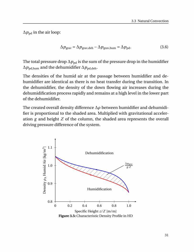
Fig. 3.5 illustrates the density profile of humid air in the humidifier andthe dehumidifier. The profile is derived from the numerical simulation (seechapter 4.3). The marked area equates to the integrals in Eq. (3.5) and isproportional to the driving pressure difference. The density differences resultfrom lower temperatures and lower humidity in the dehumidifier. The higherheat and mass transfer in the upper part of the dehumidifier dominates thedensity profile.
For steady-state conditions, this pressure difference equals the pressure drop
30
3.3 Natural Convection
∆ppd in the air loop:
∆pgrav =∆pgrav,deh −∆pgrav,hum =∆ppd. (3.6)
The total pressure drop ∆ppd is the sum of the pressure drop in the humidifier∆ppd,hum and the dehumidifier ∆ppd,deh.
The densities of the humid air at the passage between humidifier and de-humidifier are identical as there is no heat transfer during the transition. Inthe dehumidifier, the density of the down flowing air increases during thedehumidification process rapidly and remains at a high level in the lower partof the dehumidifier.
The created overall density difference ∆ρ between humidifier and dehumidi-fier is proportional to the shaded area. Multiplied with gravitational acceler-ation g and height Z of the column, the shaded area represents the overalldriving pressure difference of the system.
0.8
0.9
1.0
1.1
0 0.2 0.4 0.6 0.8 1.0
Specific Height z/Z [m/m]
Den
sity
ρA
Hu
mid
Air
[kg/
m3]
Dehumidification
Humidification
∆pgrav
g ·Z
Figure 3.5: Characteristic Density Profile in HD
31
HD Processes
3.3.4 Pressure Drop
Pressure Drop in Humidifier
For the humidifier, the pressure drop in structured packings and fillingmaterial is described by Mackowiak [64, 65].
The pressure drop depends on the velocity of water and air and the used pack-ing material. Specific data can be obtained from the manufacturer or fromliterature. For conventional packing structures in process engineering appli-cations, the pressure drop depends on the flooding point of the packing, re-spectively on the water mass flow, and the Reynolds numbers for water L andair G mass flow rate within a certain region. The flooding point of a columndefines the point, whereby the air flow G is so high that the down-flowingwater flow L is held up. In HD systems, the air flow G is always far below theflooding point for standard configurations. Mackowiak derived equations forthe different conditions within packing columns. For typical HD configura-tions, i.e. laminar water flow 0.1 < ReL < 2 and any Reynolds number ReA forthe air flow, the pressure drop for a packed column with the total height Z canbe calculated with [64, p. 271]:
∆phum
Z=ψ ·
1−ϵ
ϵ3·
u2A ·ρA
dpack ·K·
(
1−
(3
g
)1/3
·a2/3
ϵ· (νW ·uL)1/3
)−5
. (3.7)
The resistance coefficient (pressure loss) ψ for the gas flow through the pack-ing, relative void fraction ϵ of the packing, diameter dpack of one element of thepacking, the wall factor K and the geometric surface area of packing per unitvolume a are obtained from data sheets of the packing7. The gas velocity uA isbased on the cross-sectional area of an empty column. The term in bracketson the right side of the equation is approximately 1 for the small air velocitiesin HD systems. According to Ergun’s [26] correlation using a friction factor8
accounting for viscous (i.e. laminar) and kinetic energy (i.e. turbulent) losses,
7 The wall factor K is 1 for structured packings.8 In the original publication of Ergun [26], the friction factor fV ‘represents the ratio of pressure loss to viscous
energy loss which is linear with the mass flow rate’ and is defined as fV = 150+1.75 · (NRe /(1−ϵ)). This frictionfactor with the usual definition of the Reynolds Number NRe is considered in Eq. (3.7) and (3.8).
32
3.3 Natural Convection
the resistance coefficient ψ is defined as [64, p. 118]:
ψ=150
Repack+1.75. (3.8)
For typical Reynolds numbers in HD Systems (1 < Repack < 10), the first termon the right side of Eq. (3.8) is dominant so that ψ becomes proportional tou−1
A . Accordingly, the pressure drop in the humidifier becomes proportionalto the velocity uA of humid air (∆phum ∼ u2
A ·Re−1), as expected for a laminarflow regime, as described by Darcy’s law [4, p. 394].
Pressure Drop in Dehumidifier
The pressure drop of the air flow in the dehumidifier depends on the usedconfiguration of the condenser surface. In [99], the pressure drop for variousconfigurations is given. For a tube bundle configuration in an aligned arrange-ment of tubes with N rows, the pressure drop is calculated according to [99, p.Lad 1-7]:
∆pdeh
N= ξ ·
ρA ·u2A
2. (3.9)
The pressure loss coefficient ξ depends on the geometric configuration ofthe tube arrangements and the Reynolds number Re. For laminar air flowthe pressure loss coefficient ξ is proportional to Re−1. For Re ≤ 10, thetemperature influence on the fluid properties and the influence of the largernumber of tube rows (N > 10) is accounted through multiplication with acorrection factor.
As air cools along the surface area, the change of the fluid properties,especially the density, needs to be accounted for. Additionally, the velocityuA,f of the free cross section at the top and the bottom of the dehumidifier arerequired for numerical investigations.
33

HD Processes
34
4 Mathematical Modeling
4.1 Overview
This chapter describes the approach used to anlayse the processes of HD,focussing on one-dimensional (1-D) simulation of both humidifier and de-humidifier.
The observations on dropwise condensation within the dehumidifier, as ob-served in chapter 5.3.1, are anticipated in this chapter. An adapted simulationapproach is introduced to account for dropwise condensation occurring in-stead of the expected film condensation.
This chapter also provides the fundamentals required to visualize heat andmass transfer relations using the concept of operating lines and tie lines. Fur-ther, the number of transfer units NTU and the height of one transfer unitHTU are discussed.
4.2 Assumptions
The humidifier and dehumidifier are investigated in the following sectionswith the numerical 1-D simulation tool Scilab© by applying adapted corre-lations for the combined heat and mass transfer outlined. Several assump-tions are applied for the development of energy balances and heat and masstransfer rates:
1. The 1-D simulation investigates heat and mass transfer as a function ofone length coordinate, the height z of the humidifier and dehumidifiercolumn.
2. The system operates in steady-state.3. The walls of the HD casing facing the surrounding are assumed to be
ideally thermally insulated, i.e. adiabatic conditions.4. Air and vapor are assumed as ideal gases. The validity of this assumption
is shown in chapter 3.1.2.
Mathematical Modeling
5. Surface areas Aα for heat transfer and Aβ for mass transfer are equal. Theadapted approach for dropwise condensation is used for the dehumidi-fier simulation. For the humidifier simulation, the effective surface ofthe packing column Aeff,pack is provided by the manufacturer (see alsochapter 5.1.3) and used as a reference for the relevant calculations [69, p.236].
6. Differences in potential and kinetic energy are neglected due to the smallheight of the system and the low velocities. This simplification relates tothe energy balances but obviously not to the pressure difference whichaccounts for the natural convection flow of the circulating humid air.
7. The temperature of the packing tpack is assumed to be equal to the bulkfeed water temperature tW. For the here investigated HD system, thepacking material has a low heat capacity. It was not the aim to use thepacking as heat storage1.
8. Changes of the effective surface areas (e.g. due to scaling) are neglected.9. Initial values for T BT , G and L are set in accordance with Fig. 4.4.
10. A replacement thickness of a water film is introduced to account for theprevailing complex dropwise condensation processes. This simple to usereplacement model is explained in chapter 4.4.3.
4.3 Modeling of the Humidifier
Evaporation is the transfer of a substance from the liquid to the vapor state attemperatures below its boiling point2. Humidification is the absorption of thisvapor by a carrier gas.
In HD desalination systems, pure water vapor is transferred from the liquidphase, usually saline water (index W) to the gaseous phase, usually humid air(index A). L refers to the mass flow rate of the liquid and G to the mass flowrate of the carrier gas (dry air).
The specific enthalpy hA of humid air3 for relative humidity ϕ ≤ 1 is the sum
1 Hassabou [40] investigates packings with high heat capacity and high thermal conductivity.2 Vaporization occurs at the boiling point of the liquid. Consequently, vaporization occurs also inside the liquid
whereas evaporation only occurs at the surface of the liquid.3 Assumption: Air and vapor are ideal gases with constant heat capacities for the regarded temperature regions.
36
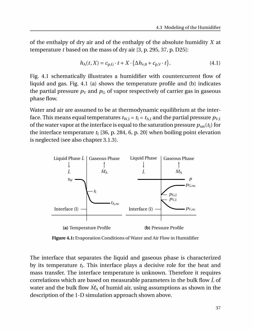
4.3 Modeling of the Humidifier
of the enthalpy of dry air and of the enthalpy of the absolute humidity X attemperature t based on the mass of dry air [3, p. 295, 37, p. D25]:
hA(t , X )= cp,G · t +X ·(
∆hv,0 + cp,V · t)
. (4.1)
Fig. 4.1 schematically illustrates a humidifier with countercurrent flow ofliquid and gas. Fig. 4.1 (a) shows the temperature profile and (b) indicatesthe partial pressure pV and pG of vapor respectively of carrier gas in gaseousphase flow.
Water and air are assumed to be at thermodynamic equilibrium at the inter-face. This means equal temperatures tW,I = tI = tA,I and the partial pressure pV,I
of the water vapor at the interface is equal to the saturation pressure psat(tI) forthe interface temperature tI [36, p. 284, 6, p. 20] when boiling point elevationis neglected (see also chapter 3.1.3).
Liquid Phase L
L
Gaseous Phase
MA
tW
Interface (I)tA,∞
tI
(a) Temperature Profile
p
pV,∞
pV,I
pG,∞
pG,I
Liquid Phase
L
Gaseous Phase
MA
Interface (I)
(b) Pressure Profile
Figure 4.1: Evaporation Conditions of Water and Air Flow in Humidifier
The interface that separates the liquid and gaseous phase is characterizedby its temperature tI. This interface plays a decisive role for the heat andmass transfer. The interface temperature is unknown. Therefore it requirescorrelations which are based on measurable parameters in the bulk flow L ofwater and the bulk flow MA of humid air, using assumptions as shown in thedescription of the 1-D simulation approach shown above.
37
Mathematical Modeling
The evaporation process comprises heat transfer due to temperature differ-ences in the liquid phase and in the gaseous phase and mass transfer due toconcentration differences of the water vapor in the gaseous phase betweeninterface (index I) and the bulk gaseous flow (index ∞). The gaseous flow canbe driven by natural or forced convection. Due to gravity forces, the liquidflows downwards in the humidifier as droplets and films on the packing so thatirregular and constantly changing interfaces between the liquid and gaseousphase are created and the liquid is continuously mixed.
4.3.1 Energy and Mass Balances
Differential equations are formed according to the mass and energy flows asdepicted in Fig. 4.2 and Fig. 4.3 to calculate process data within the humidifierover a certain differential height dz. The differential evaporated water massflow dL is:
dL = G ·dX . (4.2)
The evaporation coefficient4 σevap is defined according to Lewis, cp. [6, p. 22],as:
σevap ≡mV
XI −X∞
. (4.3)
Since non-condensable gases (NCG) are present during the humidificationand dehumidification process in HD, the unidirectional mass transfer fromthe water surface to humid air is required. The relation of the coefficient βu
for unidirectional mass transfer and the evaporation coefficient σevap can beexpressed as a function of β for equimolar mass flow and a correction factor.
This coefficient β can be determined from analogies between heat, mass andmomentum transfer [36, p. 350 ff.]5:
β=βu
p·
pV,I −pV,∞
lnp−pV,∞
p−pV,I
=βu
p·
pG,∞−pG,I
lnpG,∞
pG,I
. (4.4)
4 In some publications, such as the VDI Wärmeatlas [99], the evaporation coefficient σevap is referred to as βX.5 Grigull [36] labels βh as the mass transfer coefficient for unidirectional diffusion at the semipermeable wall.
38
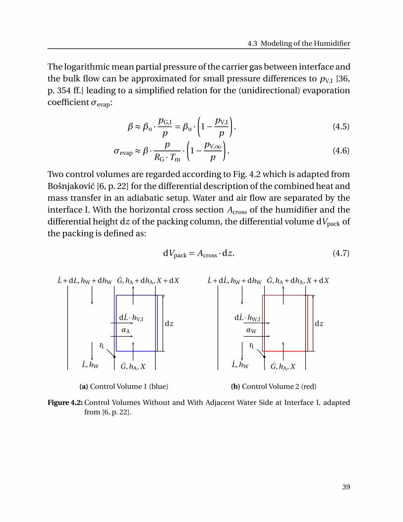
4.3 Modeling of the Humidifier
The logarithmic mean partial pressure of the carrier gas between interface andthe bulk flow can be approximated for small pressure differences to pV,I [36,p. 354 ff.] leading to a simplified relation for the (unidirectional) evaporationcoefficient σevap:
β≈βu ·pG,I
p=βu ·
(
1−pV,I
p
)
. (4.5)
σevap ≈β ·p
RG ·Tm·
(
1−pV,∞
p
)
. (4.6)
Two control volumes are regarded according to Fig. 4.2 which is adapted fromBosnjakovic [6, p. 22] for the differential description of the combined heat andmass transfer in an adiabatic setup. Water and air flow are separated by theinterface I. With the horizontal cross section Across of the humidifier and thedifferential height dz of the packing column, the differential volume dVpack ofthe packing is defined as:
dVpack = Across ·dz. (4.7)
L+dL,hW +dhW
L,hW
tI
G,hA, X
G,hA +dhA, X +dX
αA
dL ·hV,Idz
(a) Control Volume 1 (blue)
L+dL,hW +dhW
L,hW
tI
G,hA, X
G,hA +dhA, X +dX
dL ·hW,I
αWdz
(b) Control Volume 2 (red)
Figure 4.2: Control Volumes Without and With Adjacent Water Side at Interface I, adaptedfrom [6, p. 22].
39
Mathematical Modeling
The differential heat and mass transfer surface dAα and dAβ can be definedby the specific surface areas6 aα respectively aβ:
dAα = aα ·dVpack = aα · Across ·dz (4.8)
dAβ = aβ ·dVpack = aβ · Across ·dz. (4.9)
Control volume 1 contains only humid air. The energy balance for controlvolume 1 is:
G ·dhA =αA · (tI− tA,∞) ·dAα+dL ·hV,I. (4.10)
The enthalpy increase7 of humid air is the sum of the transferred heat dQA
from the interface and the enthalpy of the evaporated water with the specificenthalpy hV,I. In case of saline water, the enthalpy hV,I contains the supersat-uration resulting from the boiling point elevation cp,v ·BPE , as discussed inFig. 3.1. Thus, the enthalpy of saturated vapor h′′(tI) can be used, see also [97,p. 245].
The control volume 2 contains the humid air and is limited by a surfaceadjacent to the interface I at the water side. The energy balance of controlvolume 2 leads to the enthalpy change8 of the liquid which is equal to thetransferred enthalpy from liquid to humid air:
G ·dhA = L ·dhW+dL ·hW =αW · (tW− tI) ·dAα+dL ·hW,I. (4.11)
The increase of enthalpy of humid air is equal to the sum of heat transferred tothe interface and the enthalpy of the liquid water evaporating at the interface.Equation Eq. (4.10) and Eq. (4.11) correspond to the general energy equationfor a two component (vapor and dry air) system in steady-state flow wherekinetic energy differences and the effect of gravity and shear forces are ne-glected. Combining Eq. (4.10) and Eq. (4.11) leads to:
αW · (tW − tI) ·dAα =αA · (tI − tW,∞) ·dAα+dL · (hV,I −hW,I). (4.12)
Eq. (4.12) corresponds to Bosnjakovic [6, p. 23, Eq. (58)] and is similar to theequation stated by Treybal [97, p. 245, Eq. (7-41)]9.6 The so called effective interfacial area per unit volume a [34, p. 14-89] is also named as specific surface area (for
packing columns).7 Using Eq. (4.1) leads to: dhA = cp,G ·dt +dX ·∆hV,0 +X ·cp,V ·dt = (cp,G +X ·cp,V) ·dt +dX ·∆hV,0.8 d(L ·hW) = L ·dhW +dL ·hW.
40
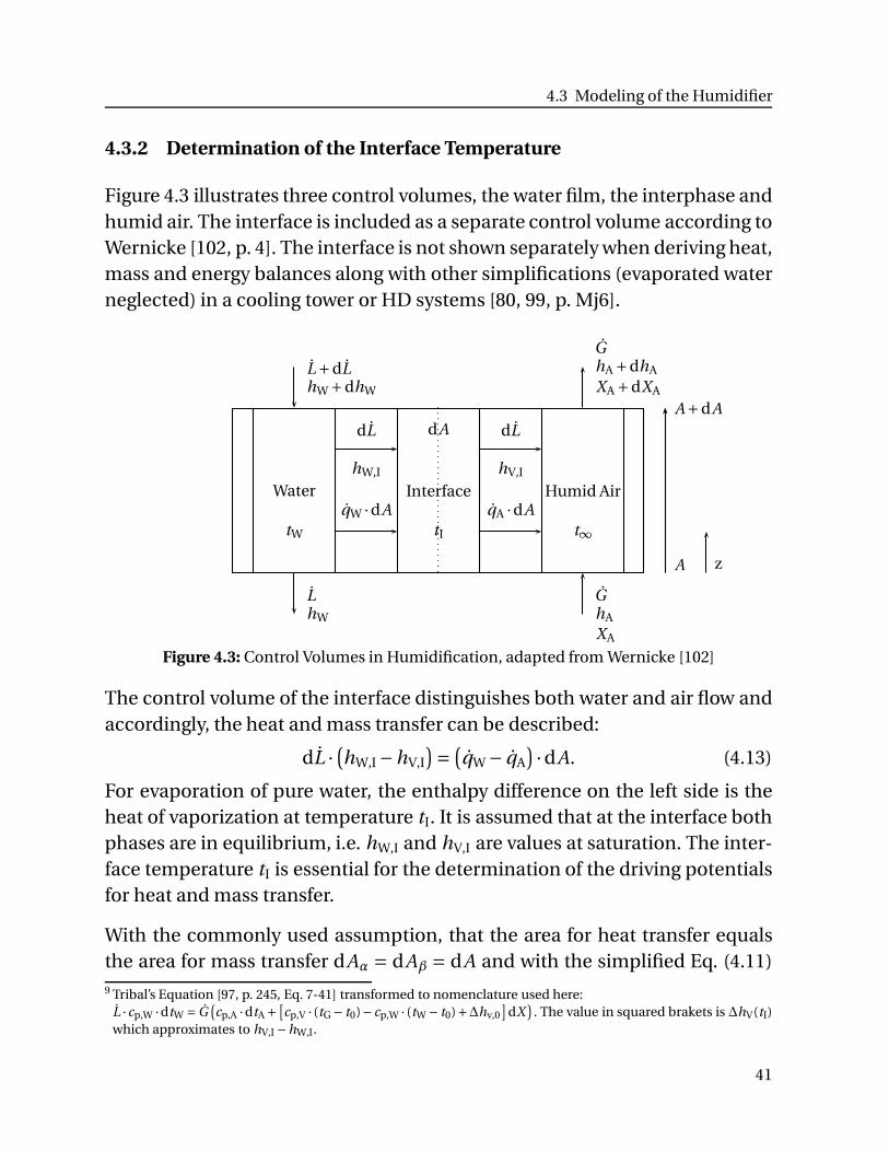
4.3 Modeling of the Humidifier
4.3.2 Determination of the Interface Temperature
Figure 4.3 illustrates three control volumes, the water film, the interphase andhumid air. The interface is included as a separate control volume according toWernicke [102, p. 4]. The interface is not shown separately when deriving heat,mass and energy balances along with other simplifications (evaporated waterneglected) in a cooling tower or HD systems [80, 99, p. Mj6].
L +dLhW +dhW
Water
tW
LhW
dL
hW,I
qW ·dAInterface
tI
dA dL
hV,I
qA ·dA
GhA +dhA
XA +dXA
GhA
XA
Humid Air
t∞
A
A+dA
z
Figure 4.3: Control Volumes in Humidification, adapted from Wernicke [102]
The control volume of the interface distinguishes both water and air flow andaccordingly, the heat and mass transfer can be described:
dL ·(
hW,I −hV,I
)
=(
qW − qA
)
·dA. (4.13)
For evaporation of pure water, the enthalpy difference on the left side is theheat of vaporization at temperature tI. It is assumed that at the interface bothphases are in equilibrium, i.e. hW,I and hV,I are values at saturation. The inter-face temperature tI is essential for the determination of the driving potentialsfor heat and mass transfer.
With the commonly used assumption, that the area for heat transfer equalsthe area for mass transfer dAα = dAβ = dA and with the simplified Eq. (4.11)9 Tribal’s Equation [97, p. 245, Eq. 7-41] transformed to nomenclature used here:
L ·cp,W ·dtW = G(
cp,A ·dtA +[
cp,V · (tG − t0)−cp,W · (tW − t0)+∆hv,0]
dX)
. The value in squared brakets is ∆hV(tI)which approximates to hV,I −hW,I.
41
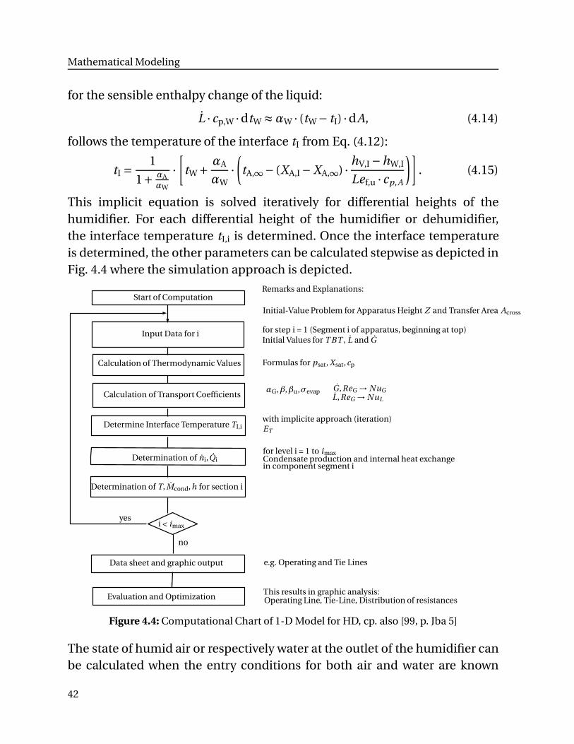
Mathematical Modeling
for the sensible enthalpy change of the liquid:
L · cp,W ·dtW ≈αW · (tW − tI) ·dA, (4.14)
follows the temperature of the interface tI from Eq. (4.12):
tI =1
1+ αAαW
·
[
tW +αA
αW·
(
tA,∞− (XA,I −XA,∞) ·hV,I −hW,I
Lef,u · cp,A
)]
. (4.15)
This implicit equation is solved iteratively for differential heights of thehumidifier. For each differential height of the humidifier or dehumidifier,the interface temperature tI,i is determined. Once the interface temperatureis determined, the other parameters can be calculated stepwise as depicted inFig. 4.4 where the simulation approach is depicted.
Start of Computation
Input Data for i
Calculation of Thermodynamic Values
Calculation of Transport Coefficients
Determine Interface Temperature TI,i
Determination of ni,Qi
Determination of T, Mcond,h for section i
i < imax
no
yes
Data sheet and graphic output
Evaluation and Optimization
Remarks and Explanations:
for step i = 1 (Segment i of apparatus, beginning at top)
Formulas for psat, Xsat,cp
αG,β,βu,σevap G,ReG → NuGL,ReG → NuL
with implicite approach (iteration)ET
for level i = 1 to imax
This results in graphic analysis:Operating Line, Tie-Line, Distribution of resistances
e.g. Operating and Tie Lines
Initial-Value Problem for Apparatus Height Z and Transfer Area Across
Initial Values for T BT , L and G
Condensate production and internal heat exchangein component segment i
Figure 4.4: Computational Chart of 1-D Model for HD, cp. also [99, p. Jba 5]
The state of humid air or respectively water at the outlet of the humidifier canbe calculated when the entry conditions for both air and water are known
42
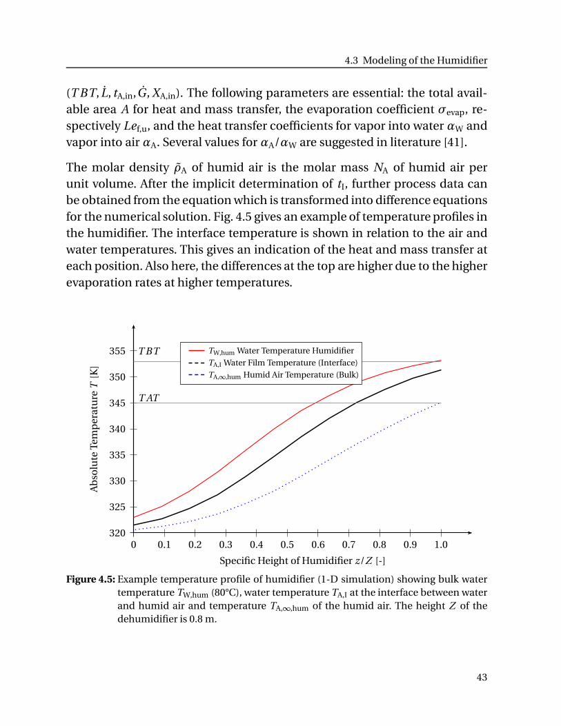
4.3 Modeling of the Humidifier
(T BT, L, tA,in,G , XA,in). The following parameters are essential: the total avail-able area A for heat and mass transfer, the evaporation coefficient σevap, re-spectively Lef,u, and the heat transfer coefficients for vapor into water αW andvapor into air αA. Several values for αA/αW are suggested in literature [41].
The molar density ρA of humid air is the molar mass NA of humid air perunit volume. After the implicit determination of tI, further process data canbe obtained from the equation which is transformed into difference equationsfor the numerical solution. Fig. 4.5 gives an example of temperature profiles inthe humidifier. The interface temperature is shown in relation to the air andwater temperatures. This gives an indication of the heat and mass transfer ateach position. Also here, the differences at the top are higher due to the higherevaporation rates at higher temperatures.
320
325
330
335
340
345
350
355
0 0.1 0.2 0.3 0.4 0.5 0.6 0.7 0.8 0.9 1.0
Specific Height of Humidifier z/Z [-]
Ab
solu
teTe
mp
erat
ure
T[K
]
T BT
T AT
TW,hum Water Temperature Humidifier
TA,I Water Film Temperature (Interface)TA,∞,hum Humid Air Temperature (Bulk)
Figure 4.5: Example temperature profile of humidifier (1-D simulation) showing bulk watertemperature TW,hum (80°C), water temperature TA,I at the interface between waterand humid air and temperature TA,∞,hum of the humid air. The height Z of thedehumidifier is 0.8 m.
43
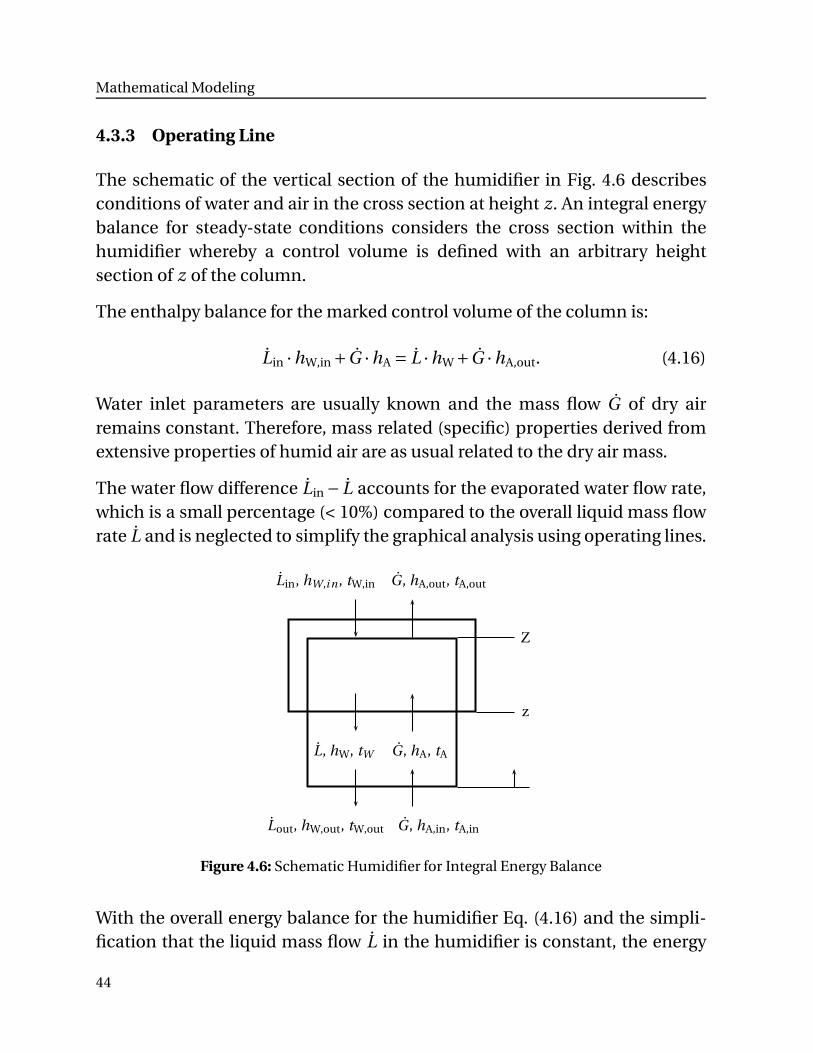
Mathematical Modeling
4.3.3 Operating Line
The schematic of the vertical section of the humidifier in Fig. 4.6 describesconditions of water and air in the cross section at height z. An integral energybalance for steady-state conditions considers the cross section within thehumidifier whereby a control volume is defined with an arbitrary heightsection of z of the column.
The enthalpy balance for the marked control volume of the column is:
Lin ·hW,in+G ·hA = L ·hW+G ·hA,out. (4.16)
Water inlet parameters are usually known and the mass flow G of dry airremains constant. Therefore, mass related (specific) properties derived fromextensive properties of humid air are as usual related to the dry air mass.
The water flow difference Lin − L accounts for the evaporated water flow rate,which is a small percentage (< 10%) compared to the overall liquid mass flowrate L and is neglected to simplify the graphical analysis using operating lines.
Lin, hW,i n , tW,in
L, hW, tW
Lout, hW,out, tW,out G , hA,in, tA,in
G, hA, tA
G, hA,out, tA,out
Z
z
Figure 4.6: Schematic Humidifier for Integral Energy Balance
With the overall energy balance for the humidifier Eq. (4.16) and the simpli-fication that the liquid mass flow L in the humidifier is constant, the energy
44
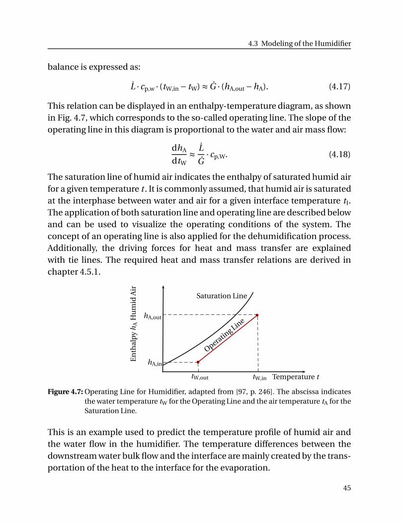
4.3 Modeling of the Humidifier
balance is expressed as:
L · cp,w · (tW,in − tW) ≈ G · (hA,out−hA). (4.17)
This relation can be displayed in an enthalpy-temperature diagram, as shownin Fig. 4.7, which corresponds to the so-called operating line. The slope of theoperating line in this diagram is proportional to the water and air mass flow:
dhA
dtW≈
L
G· cp,W. (4.18)
The saturation line of humid air indicates the enthalpy of saturated humid airfor a given temperature t . It is commonly assumed, that humid air is saturatedat the interphase between water and air for a given interface temperature tI.The application of both saturation line and operating line are described belowand can be used to visualize the operating conditions of the system. Theconcept of an operating line is also applied for the dehumidification process.Additionally, the driving forces for heat and mass transfer are explainedwith tie lines. The required heat and mass transfer relations are derived inchapter 4.5.1.
Temperature t
En
thal
py
hA
Hu
mid
Air
Operating Lin
e
Saturation Line
tW,intW,out
hA,out
hA,in
Figure 4.7: Operating Line for Humidifier, adapted from [97, p. 246]. The abscissa indicatesthe water temperature tW for the Operating Line and the air temperature tA for theSaturation Line.
This is an example used to predict the temperature profile of humid air andthe water flow in the humidifier. The temperature differences between thedownstream water bulk flow and the interface are mainly created by the trans-portation of the heat to the interface for the evaporation.
45
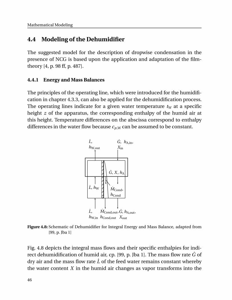
Mathematical Modeling
4.4 Modeling of the Dehumidifier
The suggested model for the description of dropwise condensation in thepresence of NCG is based upon the application and adaptation of the film-theory [4, p. 98 ff, p. 487].
4.4.1 Energy and Mass Balances
The principles of the operating line, which were introduced for the humidifi-cation in chapter 4.3.3, can also be applied for the dehumidification process.The operating lines indicate for a given water temperature tW at a specificheight z of the apparatus, the corresponding enthalpy of the humid air atthis height. Temperature differences on the abscissa correspond to enthalpydifferences in the water flow because cp,W can be assumed to be constant.
L,hW,out
L,hW,in
L, hW
G, hA,out,Xout
G, X , hA
G, hA,in,X in
MCond,hCond
MCond,out,hCond,out
Figure 4.8: Schematic of Dehumidifier for Integral Energy and Mass Balance, adapted from[99, p. Jba 1]
Fig. 4.8 depicts the integral mass flows and their specific enthalpies for indi-rect dehumidification of humid air, cp. [99, p. Jba 1]. The mass flow rate G ofdry air and the mass flow rate L of the feed water remains constant wherebythe water content X in the humid air changes as vapor transforms into the
46
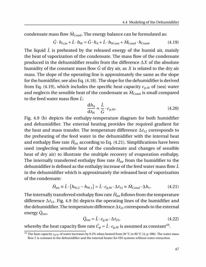
4.4 Modeling of the Dehumidifier
condensate mass flow MCond. The energy balance can be formulated as:
G ·hA,in+ L ·hW = G ·hA+ L ·hW,out+ MCond ·hCond. (4.19)
The liquid L is preheated by the released energy of the humid air, mainlythe heat of vaporization of the condensate. The mass flow of the condensateproduced in the dehumidifier results from the difference ∆X of the absolutehumidity of the constant mass flow G of dry air, as X is related to the dry airmass. The slope of the operating line is approximately the same as the slopefor the humidifier, see also Eq. (4.18). The slope for the dehumidifier is derivedfrom Eq. (4.19), which includes the specific heat capacity cp,W of (sea) waterand neglects the sensible heat of the condensate as MCond is small comparedto the feed water mass flow L:
dhA
dtW≈
L
G· cp,W. (4.20)
Fig. 4.9 (b) depicts the enthalpy-temperature diagram for both humidifierand dehumidifier. The external heating provides the required gradient forthe heat and mass transfer. The temperature difference ∆t12 corresponds tothe preheating of the feed water in the dehumidifier with the internal heatand enthalpy flow rate Hint according to Eq. (4.21). Simplifications have beenused (neglecting sensible heat of the condensate and changes of sensibleheat of dry air) to illustrate the multiple recovery of evaporation enthalpy.The internally transferred enthalpy flow rate Hint from the humidifier to thedehumidifier is defined as the enthalpy increase of the feed water mass flow Lin the dehumidifier which is approximately the released heat of vaporizationof the condensate:
Hint ≡ L ·(
hW,2 −hW,1
)
= L · cp,W ·∆t12 ≈ MCond ·∆hv. (4.21)
The internally transferred enthalpy flow rate Hint follows from the temperaturedifference ∆t12. Fig. 4.9 (b) depicts the operating lines of the humidifier andthe dehumidifier. The temperature difference∆t23 corresponds to the externalenergy Qext,
Qext = L · cp,W ·∆t23, (4.22)
whereby the heat capacity flow rate Cp = L · cp,W is assumed as constant10.10 The heat capacity cp,W of water increases by 0.3% when heated from 20 °C to 80 °C [4, p. 696]. The water mass
flow L is constant in the dehumidifier and the external heater for HD systems without water extraction.
47
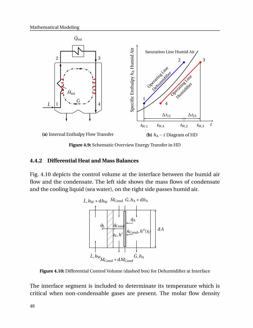
Mathematical Modeling
GL 1
2 3
4
Qext
Hint
(a) Internal Enthalpy Flow TransferSp
ecifi
cE
nth
alp
yh
AH
um
idA
ir
ttW.1 tW,2 tW,3tW,4
1
2 3
4
Operatin
g Line
Dehumid
ifier
Operatin
g Line
Humid
ifier
Saturation Line Humid Air
∆t12 ∆t23
(b) hA − t Diagram of HD
Figure 4.9: Schematic Overview Energy Transfer in HD
4.4.2 Differential Heat and Mass Balances
Fig. 4.10 depicts the control volume at the interface between the humid airflow and the condensate. The left side shows the mass flows of condensateand the cooling liquid (sea water), on the right side passes humid air.
G ,hA +dhAL,hW +dhW
L,hW
tF,h′
MCond
MCond +dMCond
qA
nCond,h′′(tI)qL qCond
G ,hA
dA
Figure 4.10: Differential Control Volume (dashed box) for Dehumidifier at Interface
The interface segment is included to determinate its temperature which iscritical when non-condensable gases are present. The molar flow density
48
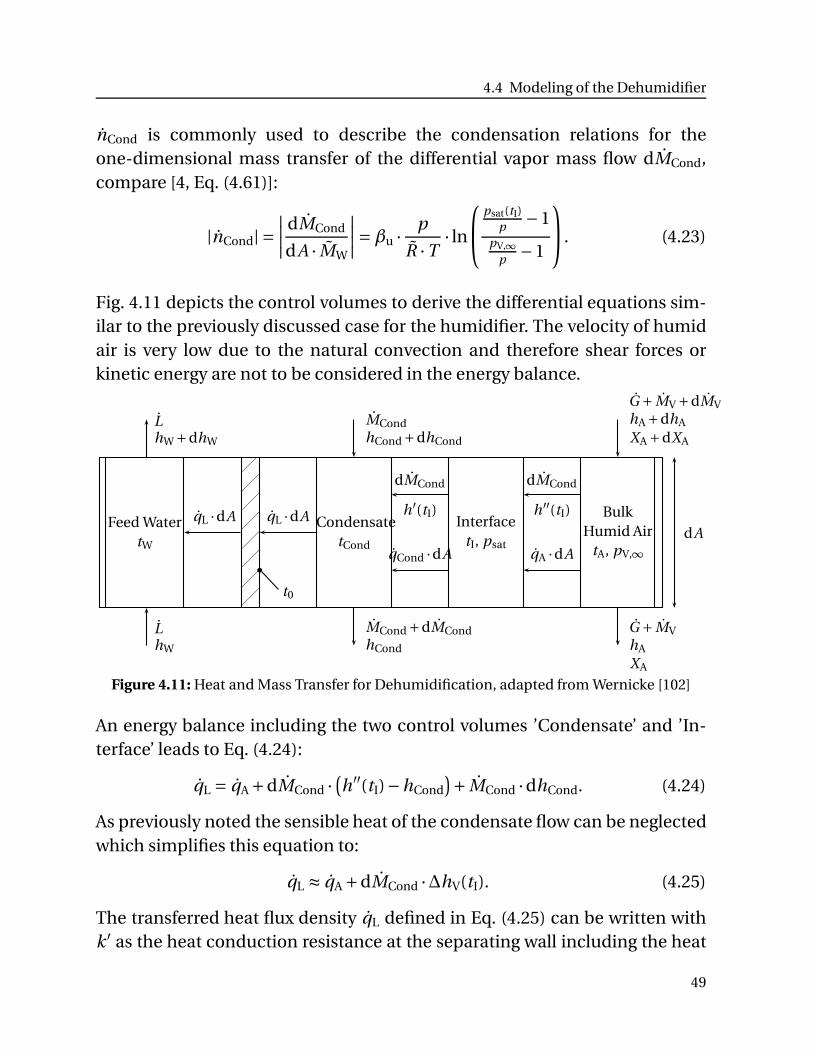
4.4 Modeling of the Dehumidifier
nCond is commonly used to describe the condensation relations for theone-dimensional mass transfer of the differential vapor mass flow dMCond,compare [4, Eq. (4.61)]:
|nCond| =
∣∣∣∣
dMCond
dA · MW
∣∣∣∣=βu ·
p
R ·T· ln
⎛
⎝
psat(tI)p −1
pV,∞
p −1
⎞
⎠ . (4.23)
Fig. 4.11 depicts the control volumes to derive the differential equations sim-ilar to the previously discussed case for the humidifier. The velocity of humidair is very low due to the natural convection and therefore shear forces orkinetic energy are not to be considered in the energy balance.
LhW +dhW
Feed WatertW
LhW
qL ·dA qL ·dA
t0
MCondhCond+dhCond
CondensatetCond
MCond +dMCondhCond
dMCond
h′(tI)
qCond ·dA
InterfacetI, psat
dMCond
h′′(tI)
qA ·dA
G + MV +dMVhA +dhA
XA +dXA
G + MVhA
XA
BulkHumid Air
tA, pV,∞
dA
Figure 4.11: Heat and Mass Transfer for Dehumidification, adapted from Wernicke [102]
An energy balance including the two control volumes ’Condensate’ and ’In-terface’ leads to Eq. (4.24):
qL = qA +dMCond ·(
h′′(tI)−hCond
)
+ MCond ·dhCond. (4.24)
As previously noted the sensible heat of the condensate flow can be neglectedwhich simplifies this equation to:
qL ≈ qA +dMCond ·∆hV(tI). (4.25)
The transferred heat flux density qL defined in Eq. (4.25) can be written withk ′ as the heat conduction resistance at the separating wall including the heat
49
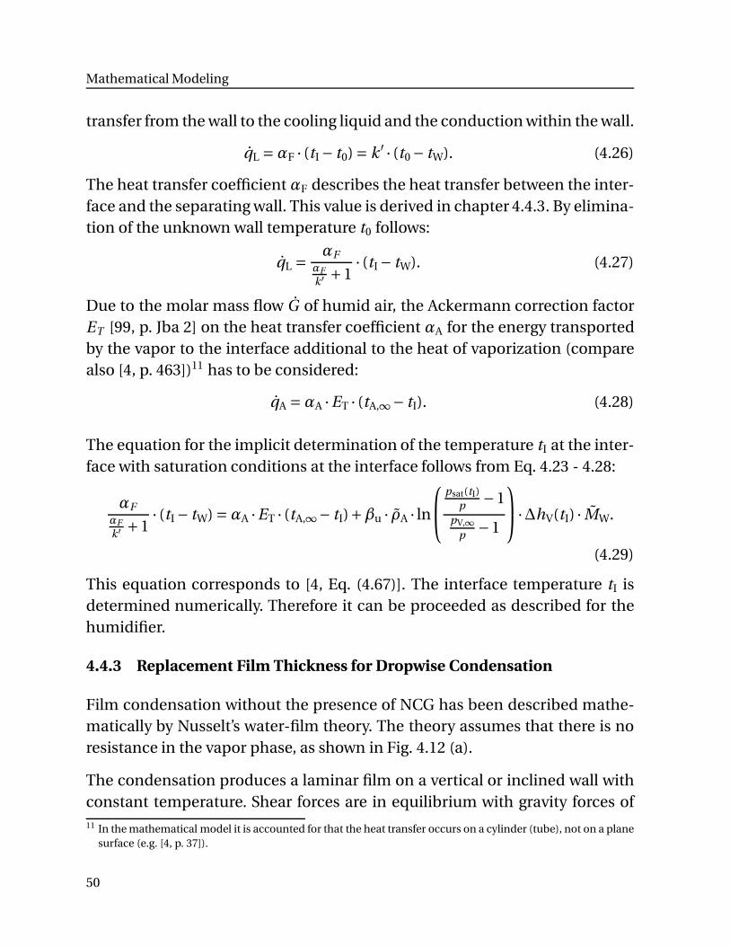
Mathematical Modeling
transfer from the wall to the cooling liquid and the conduction within the wall.
qL =αF · (tI − t0)= k ′ · (t0− tW). (4.26)
The heat transfer coefficient αF describes the heat transfer between the inter-face and the separating wall. This value is derived in chapter 4.4.3. By elimina-tion of the unknown wall temperature t0 follows:
qL =αF
αFk′ +1
· (tI − tW). (4.27)
Due to the molar mass flow G of humid air, the Ackermann correction factorET [99, p. Jba 2] on the heat transfer coefficient αA for the energy transportedby the vapor to the interface additional to the heat of vaporization (comparealso [4, p. 463])11 has to be considered:
qA =αA ·ET · (tA,∞− tI). (4.28)
The equation for the implicit determination of the temperature tI at the inter-face with saturation conditions at the interface follows from Eq. 4.23 - 4.28:
αFαFk′ +1
· (tI − tW) =αA ·ET · (tA,∞− tI)+βu · ρA · ln
⎛
⎝
psat(tI)p −1
pV,∞
p −1
⎞
⎠ ·∆hV(tI) · MW.
(4.29)
This equation corresponds to [4, Eq. (4.67)]. The interface temperature tI isdetermined numerically. Therefore it can be proceeded as described for thehumidifier.
4.4.3 Replacement Film Thickness for Dropwise Condensation
Film condensation without the presence of NCG has been described mathe-matically by Nusselt’s water-film theory. The theory assumes that there is noresistance in the vapor phase, as shown in Fig. 4.12 (a).
The condensation produces a laminar film on a vertical or inclined wall withconstant temperature. Shear forces are in equilibrium with gravity forces of11 In the mathematical model it is accounted for that the heat transfer occurs on a cylinder (tube), not on a plane
surface (e.g. [4, p. 37]).
50
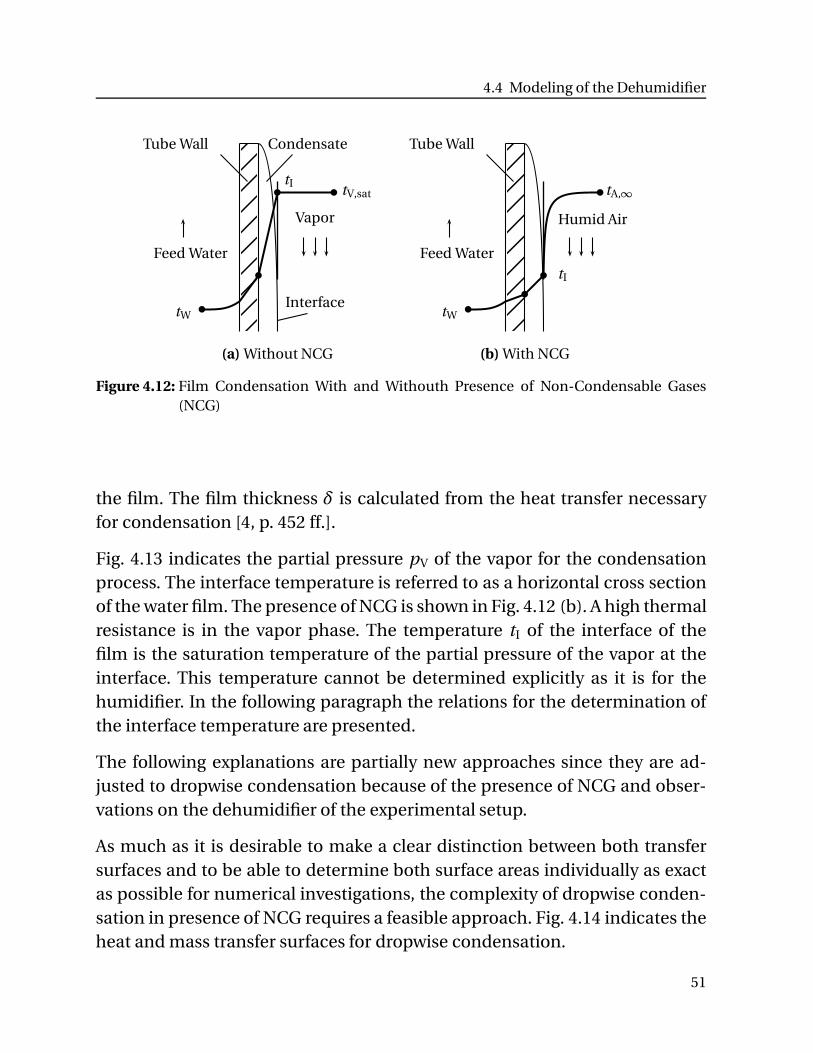
4.4 Modeling of the Dehumidifier
CondensateTube Wall
tI
Interface
Feed Water
Vapor
tW
tV,sat
(a) Without NCG
Tube Wall
tI
Feed Water
Humid Air
tW
tA,∞
(b) With NCG
Figure 4.12: Film Condensation With and Withouth Presence of Non-Condensable Gases(NCG)
the film. The film thickness δ is calculated from the heat transfer necessaryfor condensation [4, p. 452 ff.].
Fig. 4.13 indicates the partial pressure pV of the vapor for the condensationprocess. The interface temperature is referred to as a horizontal cross sectionof the water film. The presence of NCG is shown in Fig. 4.12 (b). A high thermalresistance is in the vapor phase. The temperature tI of the interface of thefilm is the saturation temperature of the partial pressure of the vapor at theinterface. This temperature cannot be determined explicitly as it is for thehumidifier. In the following paragraph the relations for the determination ofthe interface temperature are presented.
The following explanations are partially new approaches since they are ad-justed to dropwise condensation because of the presence of NCG and obser-vations on the dehumidifier of the experimental setup.
As much as it is desirable to make a clear distinction between both transfersurfaces and to be able to determine both surface areas individually as exactas possible for numerical investigations, the complexity of dropwise conden-sation in presence of NCG requires a feasible approach. Fig. 4.14 indicates theheat and mass transfer surfaces for dropwise condensation.
51
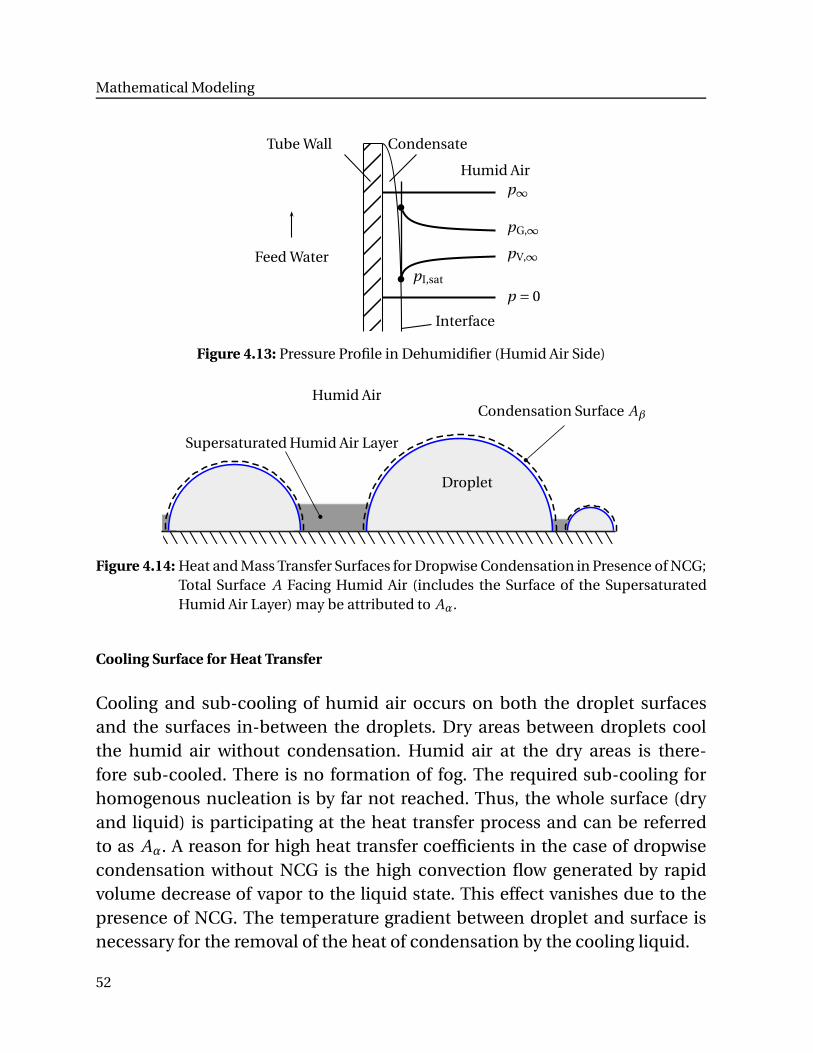
Mathematical Modeling
CondensateTube Wall
Feed Water
Interface
Humid Air
pV,∞
pI,sat
pG,∞
p∞
p = 0
Figure 4.13: Pressure Profile in Dehumidifier (Humid Air Side)
Supersaturated Humid Air Layer
Humid Air
Droplet
Condensation Surface Aβ
Figure 4.14: Heat and Mass Transfer Surfaces for Dropwise Condensation in Presence of NCG;Total Surface A Facing Humid Air (includes the Surface of the SupersaturatedHumid Air Layer) may be attributed to Aα.
Cooling Surface for Heat Transfer
Cooling and sub-cooling of humid air occurs on both the droplet surfacesand the surfaces in-between the droplets. Dry areas between droplets coolthe humid air without condensation. Humid air at the dry areas is there-fore sub-cooled. There is no formation of fog. The required sub-cooling forhomogenous nucleation is by far not reached. Thus, the whole surface (dryand liquid) is participating at the heat transfer process and can be referredto as Aα. A reason for high heat transfer coefficients in the case of dropwisecondensation without NCG is the high convection flow generated by rapidvolume decrease of vapor to the liquid state. This effect vanishes due to thepresence of NCG. The temperature gradient between droplet and surface isnecessary for the removal of the heat of condensation by the cooling liquid.
52
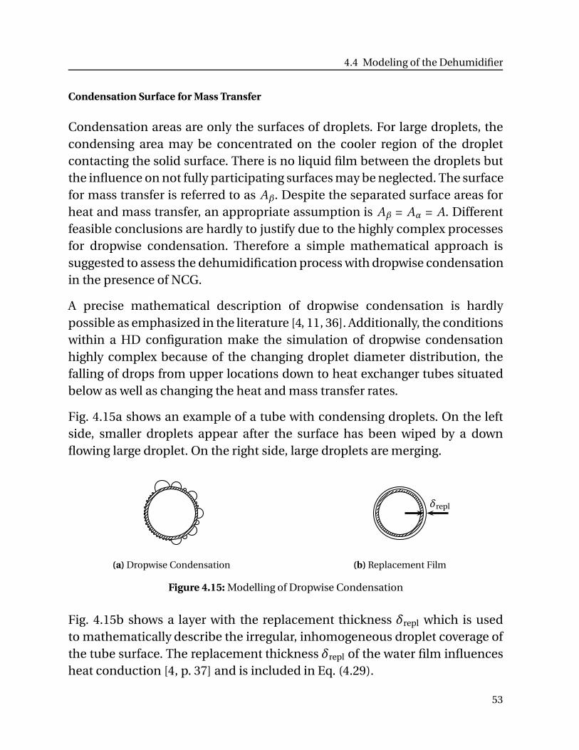
4.4 Modeling of the Dehumidifier
Condensation Surface for Mass Transfer
Condensation areas are only the surfaces of droplets. For large droplets, thecondensing area may be concentrated on the cooler region of the dropletcontacting the solid surface. There is no liquid film between the droplets butthe influence on not fully participating surfaces may be neglected. The surfacefor mass transfer is referred to as Aβ. Despite the separated surface areas forheat and mass transfer, an appropriate assumption is Aβ = Aα = A. Differentfeasible conclusions are hardly to justify due to the highly complex processesfor dropwise condensation. Therefore a simple mathematical approach issuggested to assess the dehumidification process with dropwise condensationin the presence of NCG.
A precise mathematical description of dropwise condensation is hardlypossible as emphasized in the literature [4, 11, 36]. Additionally, the conditionswithin a HD configuration make the simulation of dropwise condensationhighly complex because of the changing droplet diameter distribution, thefalling of drops from upper locations down to heat exchanger tubes situatedbelow as well as changing the heat and mass transfer rates.
Fig. 4.15a shows an example of a tube with condensing droplets. On the leftside, smaller droplets appear after the surface has been wiped by a downflowing large droplet. On the right side, large droplets are merging.
(a) Dropwise Condensation
δrepl
(b) Replacement Film
Figure 4.15: Modelling of Dropwise Condensation
Fig. 4.15b shows a layer with the replacement thickness δrepl which is usedto mathematically describe the irregular, inhomogeneous droplet coverage ofthe tube surface. The replacement thickness δrepl of the water film influencesheat conduction [4, p. 37] and is included in Eq. (4.29).
53
Mathematical Modeling
The layer of droplets remains on the tubes of the dehumidifier for a rela-tively long period which has a similar effect as a film. This approach seems tobe evident from the undertaken experimental observations allowing a feasi-ble numerical description. The phenomenon of dropwise condensation withits barrier for the heat transfer is similar. It also takes into account the rel-atively small effect of dropwise condensation on the complete dehumidifi-cation process for both heat and mass transfer.
The heat transfer coefficient αF takes into account the water film thicknessδrepl for the determination of the heat transfer in the condensate film:
αF =λW
δrepl. (4.30)
A stepwise solution of this initial-value-problem is required to calculate thedriving forces and the transport coefficients for the determination of the re-quired heat exchanger surface area. This 1-D approach corresponds to thedescribed method for the dimensioning of the humidifier whereby knowncorrelations for condensation in the presence of non-condensable gases areused. This can be done with an analysis of the condensation process and theintroduction of adequate simplifications for the mathematical description.
4.5 Visualization of Heat and Mass Transfer Relations
This section describes a way to visualize the complex relations between theprocess parameters by way of applying some simplifications.
Operating lines (see chapter 4.3.3 for the humidifier and chapter 4.4.1 forthe dehumidifier) are combined with tie lines as graphic visualization of theheat and mass transfer conditions in HD. The following description refersto the humidifier but can be transferred to the dehumidifier respectively thecomplete system.
4.5.1 Tie Line
Heat and mass transfer correlations are necessary together with mass andenergy balances for dimensioning the packing column in the humidifier. The
54
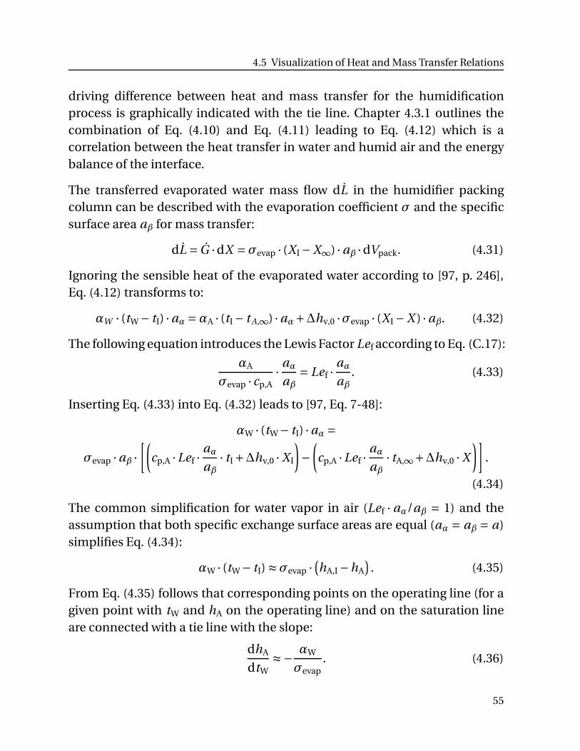
4.5 Visualization of Heat and Mass Transfer Relations
driving difference between heat and mass transfer for the humidificationprocess is graphically indicated with the tie line. Chapter 4.3.1 outlines thecombination of Eq. (4.10) and Eq. (4.11) leading to Eq. (4.12) which is acorrelation between the heat transfer in water and humid air and the energybalance of the interface.
The transferred evaporated water mass flow dL in the humidifier packingcolumn can be described with the evaporation coefficient σ and the specificsurface area aβ for mass transfer:
dL = G ·dX =σevap · (XI−X∞) ·aβ ·dVpack. (4.31)
Ignoring the sensible heat of the evaporated water according to [97, p. 246],Eq. (4.12) transforms to:
αW · (tW − tI) ·aα =αA · (tI − t A,∞) ·aα+∆hv,0 ·σevap · (XI −X ) ·aβ. (4.32)
The following equation introduces the Lewis Factor Lef according to Eq. (C.17):
αA
σevap · cp,A·
aα
aβ= Lef ·
aα
aβ. (4.33)
Inserting Eq. (4.33) into Eq. (4.32) leads to [97, Eq. 7-48]:
αW · (tW − tI) ·aα =
σevap ·aβ ·
[(
cp,A ·Lef ·aα
aβ· tI+∆hv,0 · XI
)
−
(
cp,A ·Lef ·aα
aβ· tA,∞+∆hv,0 · X
)]
.
(4.34)
The common simplification for water vapor in air (Lef · aα/aβ = 1) and theassumption that both specific exchange surface areas are equal (aα = aβ = a)simplifies Eq. (4.34):
αW · (tW − tI) ≈σevap ·(
hA,I −hA
)
. (4.35)
From Eq. (4.35) follows that corresponding points on the operating line (for agiven point with tW and hA on the operating line) and on the saturation lineare connected with a tie line with the slope:
dhA
dtW≈−
αW
σevap. (4.36)
55
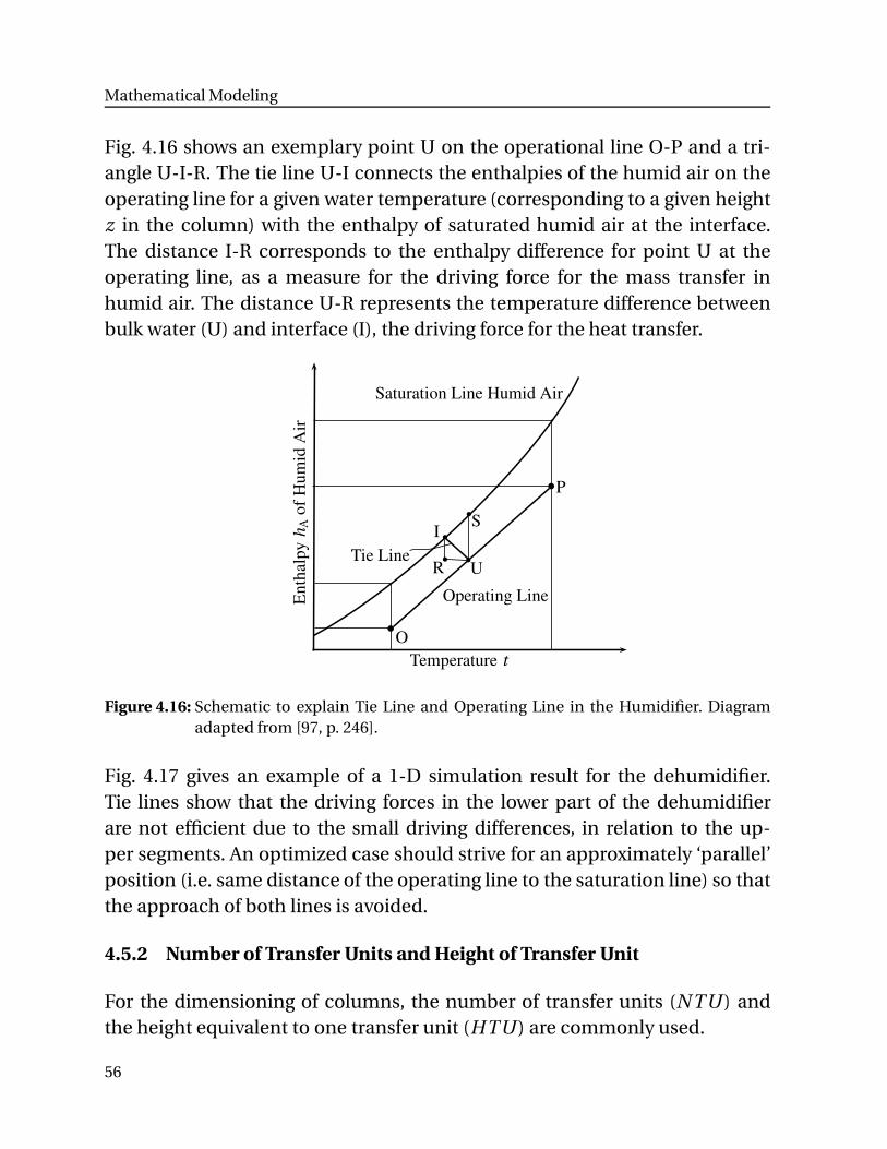
Mathematical Modeling
Fig. 4.16 shows an exemplary point U on the operational line O-P and a tri-angle U-I-R. The tie line U-I connects the enthalpies of the humid air on theoperating line for a given water temperature (corresponding to a given heightz in the column) with the enthalpy of saturated humid air at the interface.The distance I-R corresponds to the enthalpy difference for point U at theoperating line, as a measure for the driving force for the mass transfer inhumid air. The distance U-R represents the temperature difference betweenbulk water (U) and interface (I), the driving force for the heat transfer.
Temperature t
UR
IS
P
O
En
thal
py
hA
of
Hu
mid
Air
Operating Line
Saturation Line Humid Air
Tie Line
Figure 4.16: Schematic to explain Tie Line and Operating Line in the Humidifier. Diagramadapted from [97, p. 246].
Fig. 4.17 gives an example of a 1-D simulation result for the dehumidifier.Tie lines show that the driving forces in the lower part of the dehumidifierare not efficient due to the small driving differences, in relation to the up-per segments. An optimized case should strive for an approximately ‘parallel’position (i.e. same distance of the operating line to the saturation line) so thatthe approach of both lines is avoided.
4.5.2 Number of Transfer Units and Height of Transfer Unit
For the dimensioning of columns, the number of transfer units (NTU ) andthe height equivalent to one transfer unit (HTU ) are commonly used.
56
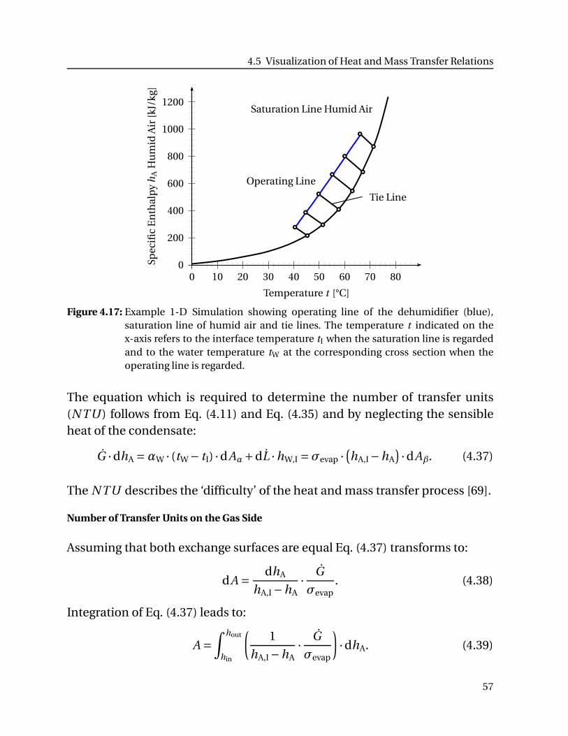
4.5 Visualization of Heat and Mass Transfer Relations
0
200
400
600
800
1000
1200
0 10 20 30 40 50 60 70 80
Temperature t [°C]
Spec
ific
En
thal
py
hA
Hu
mid
Air
[kJ/
kg]
Operating Line
Saturation Line Humid Air
Tie Line
Figure 4.17: Example 1-D Simulation showing operating line of the dehumidifier (blue),saturation line of humid air and tie lines. The temperature t indicated on thex-axis refers to the interface temperature tI when the saturation line is regardedand to the water temperature tW at the corresponding cross section when theoperating line is regarded.
The equation which is required to determine the number of transfer units(NTU ) follows from Eq. (4.11) and Eq. (4.35) and by neglecting the sensibleheat of the condensate:
G ·dhA =αW · (tW − tI) ·dAα+dL ·hW,I =σevap ·(
hA,I−hA
)
·dAβ. (4.37)
The NTU describes the ‘difficulty’ of the heat and mass transfer process [69].
Number of Transfer Units on the Gas Side
Assuming that both exchange surfaces are equal Eq. (4.37) transforms to:
dA =dhA
hA,I −hA·
G
σevap. (4.38)
Integration of Eq. (4.37) leads to:
A =
∫hout
hin
(1
hA,I−hA·
G
σevap
)
·dhA. (4.39)
57
Mathematical Modeling
If the heat transfer resistance 1/αW in the liquid phase is neglected12, thetie line matches the distance S-U in Fig. 4.16. Consequently, this enthalpydifference is used. In this case, the integral is defined only with the verticaldifference S-U (only gas side resistance). This integral is defined as thenumber of transfer units for the gas side NTUG, also referred to as theMerkel number Me. The assumption that G/σevap is constant allows thetransformation of the equation and to define the number of transfer units:
A =G
σevap·
∫hA,out
hA,in
dhA
hA,S−hA︸ ︷︷ ︸
N TUG
, (4.40)
NTUG ≡
∫hA,out
hA,in
dhA
hA,S−hA. (4.41)
This simplification can also be applied if 1/αW can not be neglected. In thiscase, the transfer coefficient σevap is adjusted accordingly.
Height Equivalent to one Transfer Unit on the Gas Side
With A = V · apack and V = Across · Z leads to the equation for the height Z ofthe transfer column:
Z =1
Across ·apack·
G
σevap︸ ︷︷ ︸
HTUG
·
∫hA,out
hA,in
dhA
hA,S−hA= HTUG ·NTUG. (4.42)
The integral on the right side of Eq. (4.42) can be graphically analyzed [6, p. 64]to determine NTUG. This equation defines the height HTUG of one transferunit. The volume Vpack of the column can therefore be calculated for a givencross section Across according to:
Vpack = Z · Across = (HTUG ·NTUG) · Across. (4.43)
The simplification can lead to considerable deviations. Therefore a detailednumerical investigation of HTU is not recommended. But, the heat and mass12 The Merkel-approach uses this assumption [68].
58
4.5 Visualization of Heat and Mass Transfer Relations
transfer relations within the HD system are visualized and unfavourable con-ditions or dimensions are displayed by applying this concept.
Numerical HD models which are based on overall energy and mass balancesfor the top and the bottom of the columns are incapable to diagnose prob-lematic heat and mass transfer conditions along the height of the column. Theusage of logarithmic mean values to simplify computation [82] hides the factthat there may be segments of the columns in which NTU are very large.
The numerical approach outlined in this chapter considers the actual oc-curring driving force along the height of the humidifier and dehumidifiercolumns. They are based on the conditions at the interface between waterand humid air.
Seifert [90, 91] reports the good agreement of the numerical simulationwith experimental results. Chapter 6 applies the here described visualizationapproach for the interpretation of experimental results provided in the nextchapter.
59

Mathematical Modeling
60
5 Experimental Investigations
The Institute for Thermodynamics at the Technische Universität München(Germany) started research on solar powered desalination in 2000 [94].Experiments on humidification processes with forced convection followed in2004. Investigations for the presented work started in 2007. Since then, severaltest rigs were designed, built, operated and optimized in the laboratory of theInstitute. Additionally, field tests in Greece in 2010 and Dubai in 2012 wereundertaken to demonstrate plant operation under real conditions. The ex-periments investigated the influence of selected operating parameters on theperformance of single and two-stage HD systems. The applied temperaturecontrol method was also tested. These long-term experiments also revealedchallenges and opportunities during setup, operation and maintenance.
5.1 Experimental Setup
5.1.1 Single and Two-Stage Configuration
Investigations on the system behavior of HD started with a single-stageclosed-air water-heated HD system setup, shown in Fig. 5.1a. After severalalterations and improvements on the system and the experimental testsetup, a two-stage closed-air water-heated HD system setup was built andtested, as shown in Fig. 5.1b. The main parameters and ranges of operatingparameters are given in Table 5.1. Annex B contains an overview of the usedinstrumentation.
The two-stage closed-air water-heated configuration is depicted in Fig.5.1b. The total exchange surfaces in humidifier and dehumidifier remainedidentical as for the single-stage setup. The testing equipment is shown inFig. 5.2. The preheated feed water from the bottom stage dehumidifier enteredthe second stage.
The schematic of the experimental single-stage test setup is shown in Fig.5.2a whereby the numbers refer to the elements exemplified in the legend.
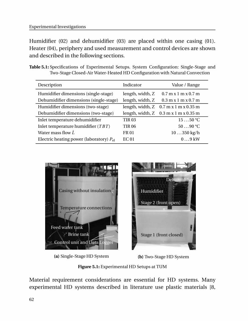
Experimental Investigations
Humidifier (02) and dehumidifier (03) are placed within one casing (01).Heater (04), periphery and used measurement and control devices are shownand described in the following sections.
Table 5.1: Specifications of Experimental Setups. System Configuration: Single-Stage andTwo-Stage Closed-Air Water-Heated HD Configuration with Natural Convection
Description Indicator Value / Range
Humidifier dimensions (single-stage) length, width, Z 0.7 m x 1 m x 0.7 m
Dehumidifier dimensions (single-stage) length, width, Z 0.3 m x 1 m x 0.7 m
Humidifier dimensions (two-stage) length, width, Z 0.7 m x 1 m x 0.35 m
Dehumidifier dimensions (two-stage) length, width, Z 0.3 m x 1 m x 0.35 m
Inlet temperature dehumidifier TIR 03 15 . . . 50 °C
Inlet temperature humidifier (T BT ) TIR 06 50 . . . 90 °C
Water mass flow L FR 01 10 . . . 350 kg/h
Electric heating power (laboratory) Pel EC 01 0 . . . 9 kW
Casing without insulation
Feed water tank
Brine tank
Control unit and Data Logger
Temperature connections
(a) Single-Stage HD System
Stage 1 (front closed)
Stage 2 (front open)
Humidifier
Dehumidifier
(b) Two-Stage HD System
Figure 5.1: Experimental HD Setups at TUM
Material requirement considerations are essential for HD systems. Manyexperimental HD systems described in literature use plastic materials [8,
62
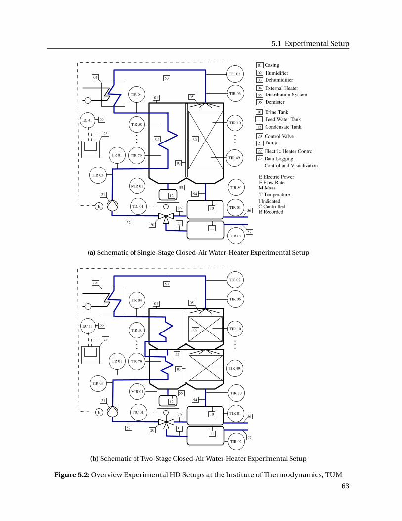
5.1 Experimental Setup
TIR 10
TIC 02
TIR 50
TIR 79TIR 49
E TIC 01
MIR 01
FR 01
TIR 01
TIR 02
TIR 04
53
TIR 06
54
03 02
04
22
12
10
11
01
20
21
52
TIR 80
EC 01
01 Casing
02 Humidifier
03 Dehumidifier
04 External Heater
23
10
50
51
55
05 05 Distribution System
56
57
Brine Tank
Pump
Feed Water Tank
Condensate Tank
Control Valve
11
12
20
21
22
23
Electric Heater Control
Data Logging,
T Temperature
M Mass
E Electric PowerF Flow Rate
I IndicatedC Controlled
Control and Visualization
R Recorded
TIR 03
06
06 Demister
(a) Schematic of Single-Stage Closed-Air Water-Heater Experimental Setup
TIR 10
TIC 02
TIR 50
TIR 79
TIR 49
E TIC 01
MIR 01
FR 01
TIR 01
TIR 02
TIR 04
53
TIR 06
54
02
04
22
12
10
11
01
20
21
52
TIR 80
EC 01
23
50
51
55
05
56
57
TIR 03
06
55
(b) Schematic of Two-Stage Closed-Air Water-Heater Experimental Setup
Figure 5.2: Overview Experimental HD Setups at the Institute of Thermodynamics, TUM
63
Experimental Investigations
40, 71, 77]. Polypropylene (PP) was selected for the casing and a majority ofthe system components as it is durable, food-safe, cost effective, corrosion-resistant [21] and suitable for operating temperatures of up to 110 °C [5, p.E68]. In addition it is resistant against hot seawater; however, operating athigh temperatures is limited by the increase of scaling and corrosion potentialand needs to be considered when choosing the operation temperature range[101].
Water Flow
For experiments in the laboratory, tap-water was used instead of seawaterto avoid corrosion on the electrical heating system. During the field tests,the system was run with local seawater. The system was operated as follows:the SHURflo (Type: 2088-313-145) diaphragm pump (21) feeds water into thetubing of the dehumidifier. The required 12 V DC voltage allows operationwith photovoltaics. The water flows inside the tubes of the dehumidifier whereit is preheated, passes the (electric or solar) heating device (04) and is spreadwith the distributor (05) onto the packing of the humidifier.
To prevent water droplets from entrainment into the dehumidifier, a demis-ter (06) is placed between humidifier and dehumidifier. The condensate isreleased into the container (12). A digital scale (MIR 01) with registration andindication records the weight of the condensate.
The brine is collected in container (10). The storage tank (11) contains feedwater. With a temperature- controlled valve (20) the mass flows of both tanksare mixed to preset set point temperature, i.e. feed water inlet temperaturetW,1, with control unit (TIC 01). The brine temperature in tank (10) increasesduring the startup phase. The transient phase is discussed and analyzed insection 5.3.2.
During this time, water is only taken from the brine container (10) until theset point temperature is reached. To keep this preset temperature, water fromthe cooler fresh water tank (11) is added. This measure reduces the time ofthe start-up phase and the influence of the inlet water temperature on theperformance ratio is investigated.
64
5.1 Experimental Setup
Another temperature control is installed for the top brine temperature T BT ,which is controlled to a preset value with the PID-control unit (TIC 02). Thecontrol unit adjusts the frequency of the pump (21) and thus the mass flow Lof the feed water.
Air Flow
The HD experimental setup is designed for natural convection air flowat ambient pressure. As mentioned in chapter 5.1.1, a demister preventsdroplet entrainment from the humidifier into the dehumidifier. Accordingto Stoke’s resistance law [37, p. B60], only very small droplets (dd < 0.1 mmfor uG = 0.2 m/s) would be carried by natural convection air flow from thehumidifier to the dehumidifier. Such small droplets may be produced whenspray nozzles for water distribution in the humidifier are used.
The water distribution system is described in chapter 5.1.3. It creates dropletsonly by gravitational and surface tension forces so that entrainment by verysmall droplets is avoided.
Setups with and without a separation wall between humidifier and dehumidi-fier were investigated, as suggested by Müller-Holst [71].
5.1.2 External Heater
An electrical water heater is used as external heater (04) for the laboratorysetup at the TUM. Solar collectors are used for field-tests in Greece and Dubai.
Electrical Water Heater
For investigations in the TUM laboratory, the test rig is equipped with acontinuous-flow water heater, manufactured by DEW Dueblein. The electricalheating power of maximum 9 kW is controlled with a power-transformer byadjusting the voltage. The system is calibrated with water temperature andwater mass flow measurements. The control system could also be configuredto trigger time-dependent changes of power to simulate solar irradiation. Thereference value for the external heating power Qext is set as 4.7 kW for all of thehere presented experimental data.
65
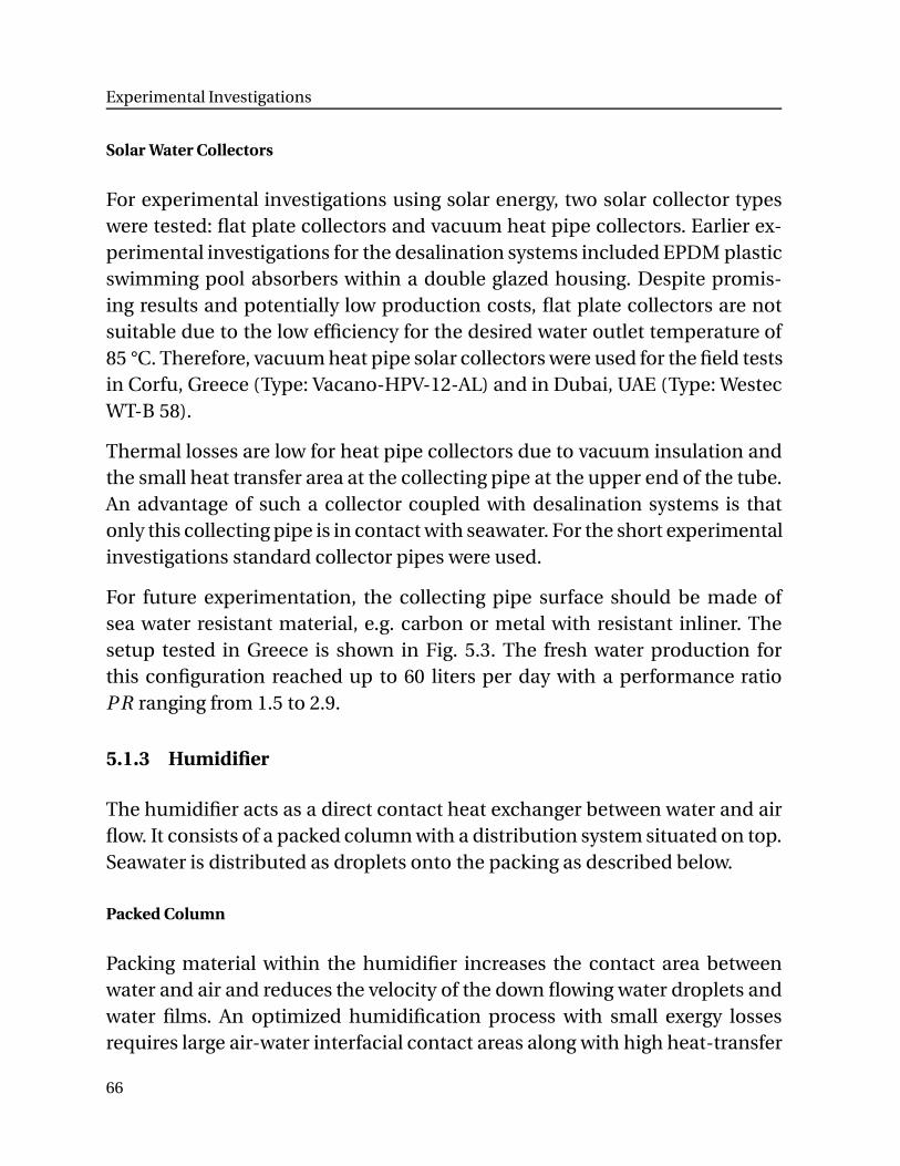
Experimental Investigations
Solar Water Collectors
For experimental investigations using solar energy, two solar collector typeswere tested: flat plate collectors and vacuum heat pipe collectors. Earlier ex-perimental investigations for the desalination systems included EPDM plasticswimming pool absorbers within a double glazed housing. Despite promis-ing results and potentially low production costs, flat plate collectors are notsuitable due to the low efficiency for the desired water outlet temperature of85 °C. Therefore, vacuum heat pipe solar collectors were used for the field testsin Corfu, Greece (Type: Vacano-HPV-12-AL) and in Dubai, UAE (Type: WestecWT-B 58).
Thermal losses are low for heat pipe collectors due to vacuum insulation andthe small heat transfer area at the collecting pipe at the upper end of the tube.An advantage of such a collector coupled with desalination systems is thatonly this collecting pipe is in contact with seawater. For the short experimentalinvestigations standard collector pipes were used.
For future experimentation, the collecting pipe surface should be made ofsea water resistant material, e.g. carbon or metal with resistant inliner. Thesetup tested in Greece is shown in Fig. 5.3. The fresh water production forthis configuration reached up to 60 liters per day with a performance ratioP R ranging from 1.5 to 2.9.
5.1.3 Humidifier
The humidifier acts as a direct contact heat exchanger between water and airflow. It consists of a packed column with a distribution system situated on top.Seawater is distributed as droplets onto the packing as described below.
Packed Column
Packing material within the humidifier increases the contact area betweenwater and air and reduces the velocity of the down flowing water droplets andwater films. An optimized humidification process with small exergy lossesrequires large air-water interfacial contact areas along with high heat-transfer
66
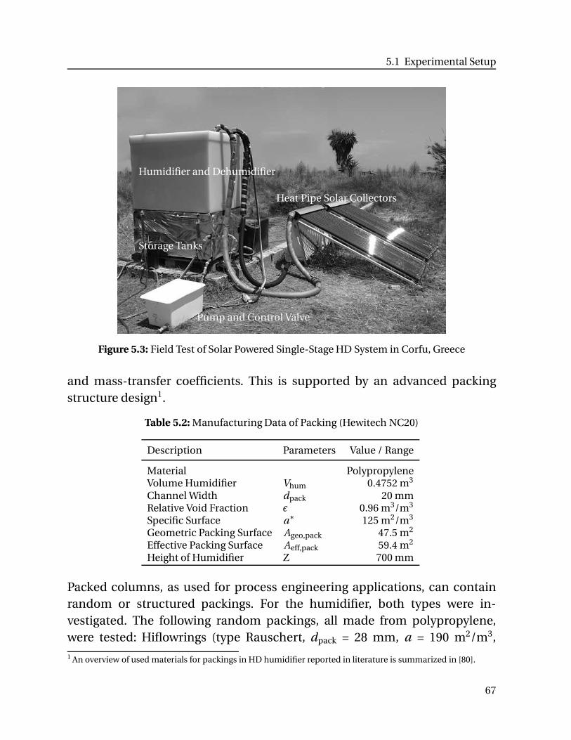
5.1 Experimental Setup
Pump and Control Valve
Storage Tanks
Humidifier and Dehumidifier
Heat Pipe Solar Collectors
Figure 5.3: Field Test of Solar Powered Single-Stage HD System in Corfu, Greece
and mass-transfer coefficients. This is supported by an advanced packingstructure design1.
Table 5.2: Manufacturing Data of Packing (Hewitech NC20)
Description Parameters Value / Range
Material PolypropyleneVolume Humidifier Vhum 0.4752 m3
Channel Width dpack 20 mmRelative Void Fraction ϵ 0.96 m3/m3
Specific Surface a∗ 125 m2/m3
Geometric Packing Surface Ageo,pack 47.5 m2
Effective Packing Surface Aeff,pack 59.4 m2
Height of Humidifier Z 700 mm
Packed columns, as used for process engineering applications, can containrandom or structured packings. For the humidifier, both types were in-vestigated. The following random packings, all made from polypropylene,were tested: Hiflowrings (type Rauschert, dpack = 28 mm, a = 190 m2/m3,
1 An overview of used materials for packings in HD humidifier reported in literature is summarized in [80].
67
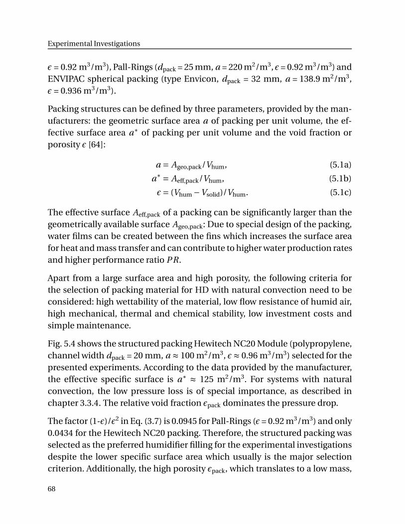
Experimental Investigations
ϵ = 0.92 m3/m3), Pall-Rings (dpack = 25 mm, a = 220 m2/m3, ϵ = 0.92 m3/m3) andENVIPAC spherical packing (type Envicon, dpack = 32 mm, a = 138.9 m2/m3,ϵ = 0.936 m3/m3).
Packing structures can be defined by three parameters, provided by the man-ufacturers: the geometric surface area a of packing per unit volume, the ef-fective surface area a∗ of packing per unit volume and the void fraction orporosity ϵ [64]:
a = Ageo,pack/Vhum, (5.1a)
a∗ = Aeff,pack/Vhum, (5.1b)
ϵ= (Vhum −Vsolid)/Vhum. (5.1c)
The effective surface Aeff,pack of a packing can be significantly larger than thegeometrically available surface Ageo,pack: Due to special design of the packing,water films can be created between the fins which increases the surface areafor heat and mass transfer and can contribute to higher water production ratesand higher performance ratio P R.
Apart from a large surface area and high porosity, the following criteria forthe selection of packing material for HD with natural convection need to beconsidered: high wettability of the material, low flow resistance of humid air,high mechanical, thermal and chemical stability, low investment costs andsimple maintenance.
Fig. 5.4 shows the structured packing Hewitech NC20 Module (polypropylene,channel width dpack = 20 mm, a ≈ 100 m2/m3, ϵ≈ 0.96 m3/m3) selected for thepresented experiments. According to the data provided by the manufacturer,the effective specific surface is a∗ ≈ 125 m2/m3. For systems with naturalconvection, the low pressure loss is of special importance, as described inchapter 3.3.4. The relative void fraction ϵpack dominates the pressure drop.
The factor (1-ϵ)/ϵ2 in Eq. (3.7) is 0.0945 for Pall-Rings (ϵ = 0.92 m3/m3) and only0.0434 for the Hewitech NC20 packing. Therefore, the structured packing wasselected as the preferred humidifier filling for the experimental investigationsdespite the lower specific surface area which usually is the major selectioncriterion. Additionally, the high porosity ϵpack, which translates to a low mass,
68
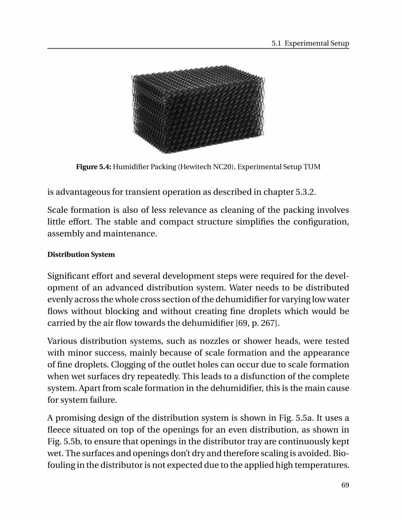
5.1 Experimental Setup
Figure 5.4: Humidifier Packing (Hewitech NC20), Experimental Setup TUM
is advantageous for transient operation as described in chapter 5.3.2.
Scale formation is also of less relevance as cleaning of the packing involveslittle effort. The stable and compact structure simplifies the configuration,assembly and maintenance.
Distribution System
Significant effort and several development steps were required for the devel-opment of an advanced distribution system. Water needs to be distributedevenly across the whole cross section of the dehumidifier for varying low waterflows without blocking and without creating fine droplets which would becarried by the air flow towards the dehumidifier [69, p. 267].
Various distribution systems, such as nozzles or shower heads, were testedwith minor success, mainly because of scale formation and the appearanceof fine droplets. Clogging of the outlet holes can occur due to scale formationwhen wet surfaces dry repeatedly. This leads to a disfunction of the completesystem. Apart from scale formation in the dehumidifier, this is the main causefor system failure.
A promising design of the distribution system is shown in Fig. 5.5a. It uses afleece situated on top of the openings for an even distribution, as shown inFig. 5.5b, to ensure that openings in the distributor tray are continuously keptwet. The surfaces and openings don’t dry and therefore scaling is avoided. Bio-fouling in the distributor is not expected due to the applied high temperatures.
69
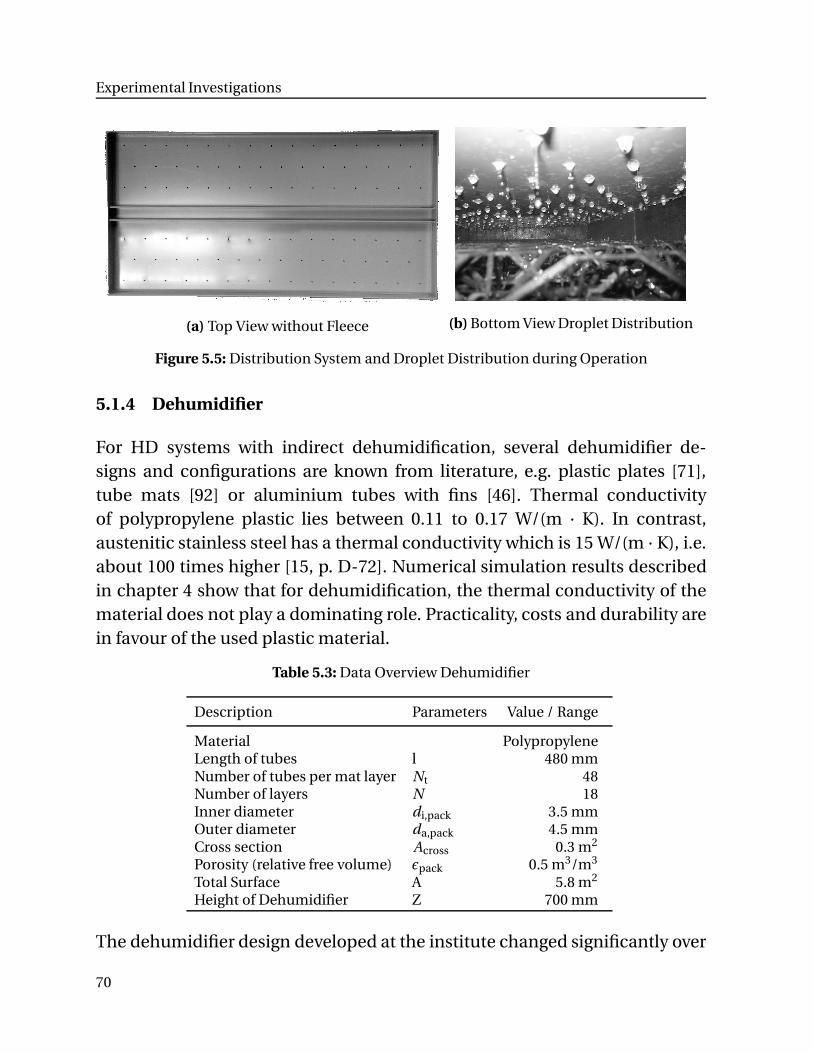
Experimental Investigations
(a) Top View without Fleece (b) Bottom View Droplet Distribution
Figure 5.5: Distribution System and Droplet Distribution during Operation
5.1.4 Dehumidifier
For HD systems with indirect dehumidification, several dehumidifier de-signs and configurations are known from literature, e.g. plastic plates [71],tube mats [92] or aluminium tubes with fins [46]. Thermal conductivityof polypropylene plastic lies between 0.11 to 0.17 W/(m · K). In contrast,austenitic stainless steel has a thermal conductivity which is 15 W/(m · K), i.e.about 100 times higher [15, p. D-72]. Numerical simulation results describedin chapter 4 show that for dehumidification, the thermal conductivity of thematerial does not play a dominating role. Practicality, costs and durability arein favour of the used plastic material.
Table 5.3: Data Overview Dehumidifier
Description Parameters Value / Range
Material PolypropyleneLength of tubes l 480 mmNumber of tubes per mat layer Nt 48Number of layers N 18Inner diameter di,pack 3.5 mmOuter diameter da,pack 4.5 mmCross section Across 0.3 m2
Porosity (relative free volume) ϵpack 0.5 m3/m3
Total Surface A 5.8 m2
Height of Dehumidifier Z 700 mm
The dehumidifier design developed at the institute changed significantly over
70
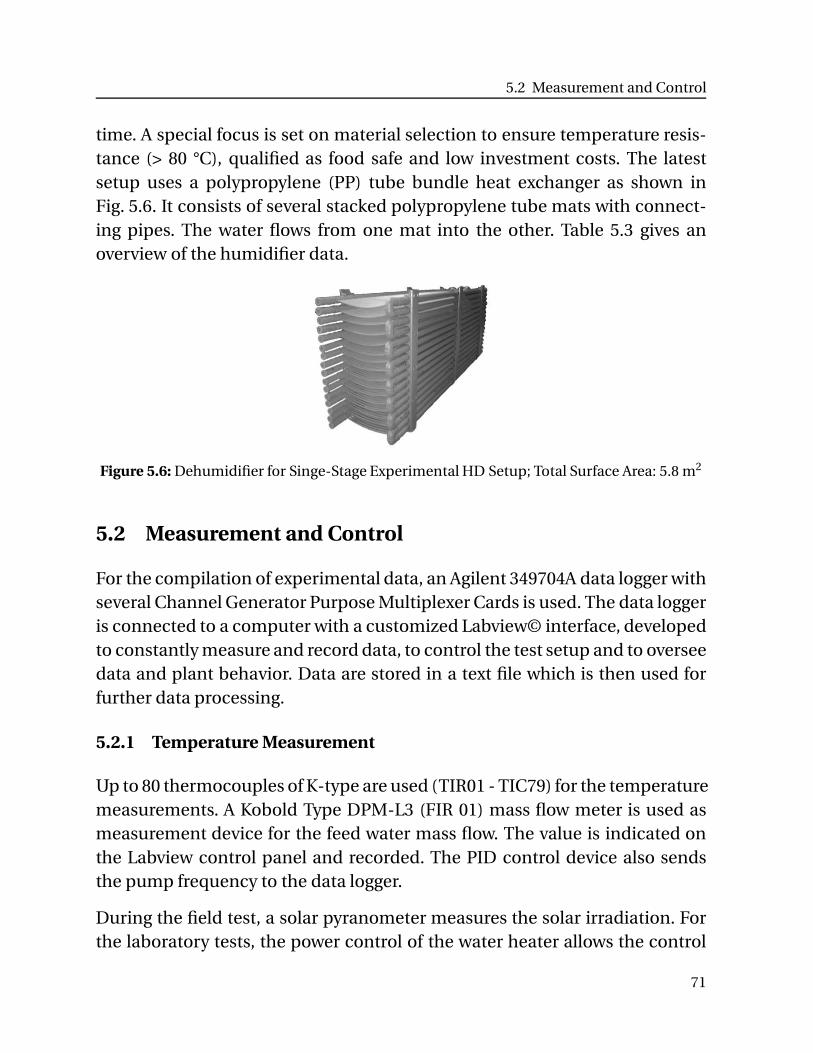
5.2 Measurement and Control
time. A special focus is set on material selection to ensure temperature resis-tance (> 80 °C), qualified as food safe and low investment costs. The latestsetup uses a polypropylene (PP) tube bundle heat exchanger as shown inFig. 5.6. It consists of several stacked polypropylene tube mats with connect-ing pipes. The water flows from one mat into the other. Table 5.3 gives anoverview of the humidifier data.
Figure 5.6: Dehumidifier for Singe-Stage Experimental HD Setup; Total Surface Area: 5.8 m2
5.2 Measurement and Control
For the compilation of experimental data, an Agilent 349704A data logger withseveral Channel Generator Purpose Multiplexer Cards is used. The data loggeris connected to a computer with a customized Labview© interface, developedto constantly measure and record data, to control the test setup and to overseedata and plant behavior. Data are stored in a text file which is then used forfurther data processing.
5.2.1 Temperature Measurement
Up to 80 thermocouples of K-type are used (TIR01 - TIC79) for the temperaturemeasurements. A Kobold Type DPM-L3 (FIR 01) mass flow meter is used asmeasurement device for the feed water mass flow. The value is indicated onthe Labview control panel and recorded. The PID control device also sendsthe pump frequency to the data logger.
During the field test, a solar pyranometer measures the solar irradiation. Forthe laboratory tests, the power control of the water heater allows the control
71
Experimental Investigations
of the heat input and also the running of preset programs, e.g. to control thepower which corresponds to the solar insulation during the day.
Water temperatures in connecting ducts can be determined with high pre-cision (tW,in, tW,deh,out and tW,hum,in). Measuring the temperature of free flowingwater within the humidifier, in particular tW,hum,out, is challenging and is mea-sured with far less precision. Errors also occur due to the transient behaviorof the system. These errors can be reduced by reproducing experiments andaveraging the results. For experimental results, a minimum of five experimen-tal test runs have been obtained. The accuracy of single temperature measure-ments lies between ± 1 °C.
Measurements of the humid air temperature have a lower accuracy than thewater temperatures because condensing water vapor falsifies the results. Intheir report Seifert et al. [91, p. 12, Fig. 6] published a deviation of ± 1.8 Kbetween the measured temperatures of humid air and the temperatures fromthe simulation of the studied dehumidification. A temperature differencecorresponds to a deviation of the saturation humidity Xsat. The mean slope∆Xsat/∆t of the saturation line in the temperature region of 40.5 °C to 75 °C is0.0123 1/K. Therefore a temperature error of ± 1.8 K results in a deviation ofthe absolute humidity of 0.022 kg/kg.
5.2.2 Condensate Mass Flow Rate Measurement
A digital scale is connected to the data logging unit to determine the con-densate mass flow MCond from the recording in the given time. The conden-sate mass flow and the external heat input Qext are the necessary values forthe determination of the Performance Ratio P R. It was initially assumed thatthe condensate mass flow can be determined with a satisfactory accuracy tointerpret the measured data to draw conclusions regarding the overall effectof improvement measures. The water quality is determined manually with aconductivity measurement device (BC-Electronics, Model C135).
It became evident from the numerical investigations of the Performance RatioP R, as shown in the next chapter, that the error is possibly in the range of 20%because the small amounts of water may not be detected correctly by the scale
72
5.2 Measurement and Control
within the selected time frame as any physical contact with the system causingvibration of the dehumidifier may have changed the liquid hold up.
A considerable margin of error needs to be applied to the water mass flowmeasurement data, as also shown in the next chapter where this error is fur-ther investigated by applying an adapted Performance Ratio P RHD which isbased on measurement values that can be determined with a greater certainty.
5.2.3 System Control
The aim of controlling the system is to maintain preset operating valuesduring changing conditions, e.g. the start-up or when using solar energy. Asthe preferred control strategy, T BT is selected as the main controlled processvariable with a constant set value, e.g. 85 °C.
The water mass flow is the actuating variable: the PID control unit sends adigital signal to the control unit of the pump to adjust the stroke frequencyand the water mass flow respectively. The control unit (manufacturer: PMA,Model: ECO24) adjusts the system according to the solar radiation when op-erated with solar collectors. This control mechanism was found to be advan-tageous compared to the alternative, whereby the mass flow rate remainsconstant for a given external heat input, leading to changing T BT during op-eration. For significant change in irradiation, e.g. a moving cloud, the systemwould rapidly cool down resulting in a significant loss in production due tothe additional starting-up phase in these time periods.
When coupling the system with a heat source with a constant temperatureover a long period (e.g. waste heat from other processes) it may be advan-tageous to set the water mass flow to a constant value whereas for a transientheat input (solar power) the T BT may be set as a constant value.
The operation temperature region, at which humidification takes place, isdependent on the temperature tW,in (i.e. TIR 03 in Fig. 5.2) of the feed waterflow into the dehumidifier. This temperature can be adjusted, given a constantsea water feed temperature, by mixing the cool sea water with brine. This ofcourse is limited by the concentration and the scaling behavior.
73
Experimental Investigations
With increased Qext, the necessary heat and mass transfer surfaces can bereduced for a given condensate output as the driving temperature differenceincreases. This obviously reduces the performance ratio; however, investmentcost can be reduced if Qext is increased due to higher irradiation. TW,in is nota direct function of the external heat input but depends on the available feedwater temperature and optional blending with available brine to recover avail-able heat from the brine and reduce water input.
A system consisting of a water tank (10) for brine recirculation, a feedwater tank (11) with cool water (may be replaced by a direct intake fromthe water source) in combination with a three-way temperature valve (20)for temperature regulation stabilizes the system’s behavior. With the valve,the inlet temperature into the dehumidifier is controlled. Seifert et al. [91]describes this setup (with a similar recirculation approach) in the same yearas Soufari et al. [93].
During the start-up phase, water is recirculated within the system, i.e. a close-air closed-water configuration where no water from the feed water tank (11)is used. As soon as the inlet water temperature tin reaches the value set forTIC 01 the system changes to an open-water configuration, i.e. the controlvalve (20) opens and cooler water from the feed water tank (11) is mixed withwater from the brine water tank (10). The pump (21) requires a certain waterlevel within the brine tank (10), i.e. the inlet feed water tin temperature is lowerthan the humidifier outlet temperature tW,hum,out. Therefore, the closed-waterconfiguration during the start-up phases could not be used to its full potentialdue to technical limitations.
5.3 Experimental Results and Observations
5.3.1 Dropwise Condensation
The here distinguished condensation process considers the conditions withina closed-air HD setup with natural convection with a polypropylene tubebundle dehumidifier. The findings concerning dropwise condensation onplastic tubes (PP) may not be adaptable to other configurations or materials.
74
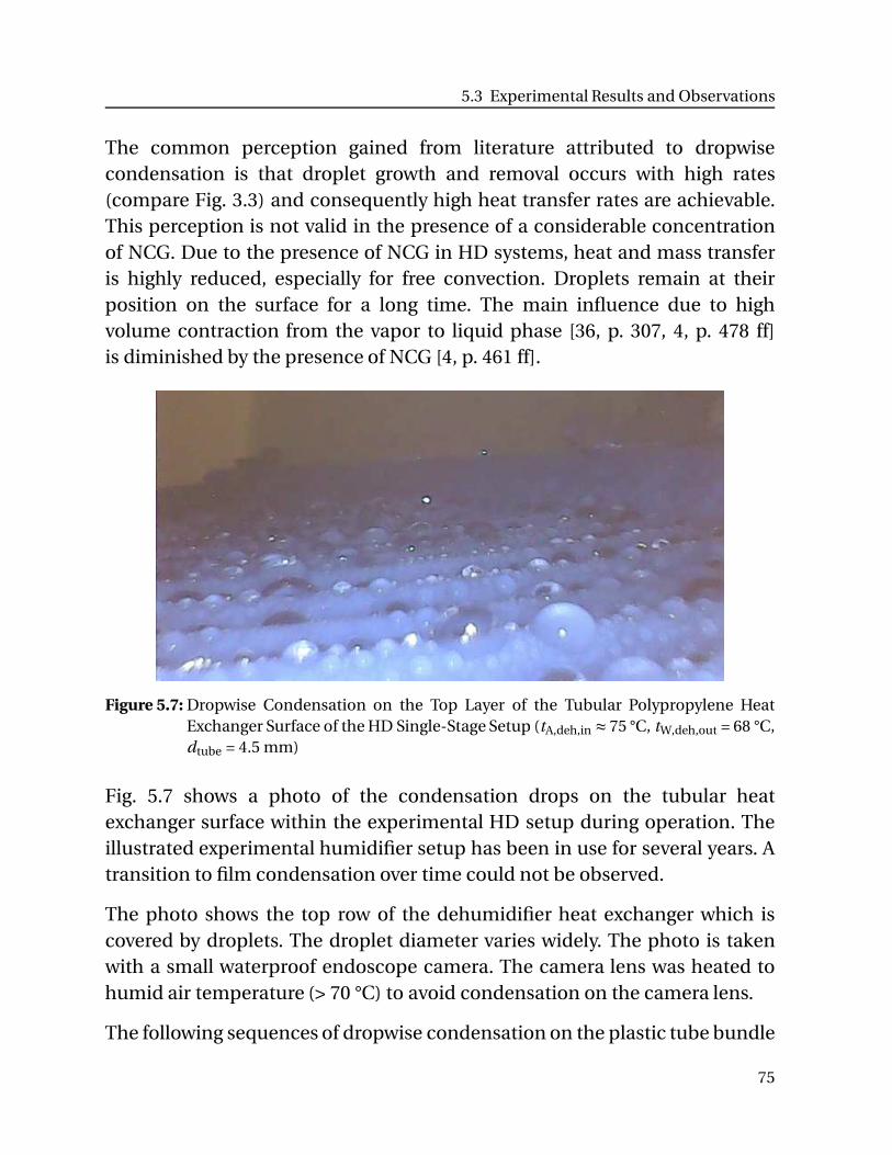
5.3 Experimental Results and Observations
The common perception gained from literature attributed to dropwisecondensation is that droplet growth and removal occurs with high rates(compare Fig. 3.3) and consequently high heat transfer rates are achievable.This perception is not valid in the presence of a considerable concentrationof NCG. Due to the presence of NCG in HD systems, heat and mass transferis highly reduced, especially for free convection. Droplets remain at theirposition on the surface for a long time. The main influence due to highvolume contraction from the vapor to liquid phase [36, p. 307, 4, p. 478 ff]is diminished by the presence of NCG [4, p. 461 ff].
Figure 5.7: Dropwise Condensation on the Top Layer of the Tubular Polypropylene HeatExchanger Surface of the HD Single-Stage Setup (tA,deh,in ≈ 75 °C, tW,deh,out = 68 °C,dtube = 4.5 mm)
Fig. 5.7 shows a photo of the condensation drops on the tubular heatexchanger surface within the experimental HD setup during operation. Theillustrated experimental humidifier setup has been in use for several years. Atransition to film condensation over time could not be observed.
The photo shows the top row of the dehumidifier heat exchanger which iscovered by droplets. The droplet diameter varies widely. The photo is takenwith a small waterproof endoscope camera. The camera lens was heated tohumid air temperature (> 70 °C) to avoid condensation on the camera lens.
The following sequences of dropwise condensation on the plastic tube bundle
75
Experimental Investigations
in the dehumidifier can be observed:
1. Rolling down of a large droplet with high velocity. This clearing processon a certain area occurs within a very short time (below one second).
2. On its way, the large droplet merges with other droplets and leavesbehind a wiped trail.
3. On this trail, a high population density of small droplets appears shortlyafter.
4. Droplets grow due to condensation and due to merging with contactingdroplets (the growth process lasts several minutes).
5. Areas between the droplets seem to be dry.6. No additional droplets are created during the growth process. Merging
leads to a reduction of the number of droplets.7. During the growth process, droplets change their position only when
merging or being captured by droplets moving down.8. Some droplets become unstable, they flow down and the sequence
starts again with the clearing process. If a droplet becomes unstableas it reaches a critical size or by vibrating surfaces or by merging withanother droplet, it flows down the cooling surface.
9. Droplet motion during condensation in the dehumidifier of HD is veryslow, except during the very short processes of clearing and merging.
10. Falling droplets clashing on the below tube clears a certain area. As thiscleaning process continually occurs, the maximum droplet diameter isnot reached for the affected droplets.
Micro droplets appear at the trail of the droplet with dry patches between themicro droplets. It can be assumed that heterogeneous nucleation immediatelytakes place at the wiped surface after passing of a large droplet. There is nomore nucleation in the presence of neighbouring liquid surfaces for conden-sation at this temperature.
Droplets grow as condensate forms and by merging with smaller surroundingdroplets. Vapor condenses at the droplet surfaces from sub-cooled humidair. Condensation takes place on the liquid surface. When droplets contacteach other, the smaller droplet is incorporated by the larger droplets becausedroplets with a larger radius R have a lower inner pressure due to the surface
76
5.3 Experimental Results and Observations
tension σ, according to ∆p = 2 ·σ/R [33, p. 355]. The droplet size on the tubesurface depends on time, its position on the surface of the tube, and on theposition of the tube within the tube bundle configuration.
These findings are an important element for the mathematical description ofdropwise condensation in the HD system, as outlined in chapter 4.4.3.
5.3.2 Data Transient and Steady-State Phases
A large amount of experimental data is obtained from test runs with varioussystem parameters. Fig. 5.8 shows results of a test run with a single-stage HDsystem and Fig. 5.9 a two-stage HD system with similar operating parameters.The figures indicate experimental results collected within 10,000 seconds aftersystem start. The overall measurement time was usually chosen to be morethan seven hours to validate that condensate water production rate remainsconstant over a longer time period. The considerable total operation time ofthe system gives an indication for maintenance requirements and componentdurability.
Four operating phases are distinguished: three transient phases (I-III) and asteady-state phase (IV). All phases are distinguished by temperature transi-tions which can be identified by sharp bends. This is the preferred method,especially for phase IV, during which the determination of the steady-statetemperatures are difficult due to the marginal temperature changes.
The transition temperatures for each phase are highlighted in Fig. 5.8 (a) aspoints A, B and C. The condensate mass flow rate MCond which was measuredwith the electronic scale is not shown as experimental results are capturedover long time intervals. Measurable and meaningful results are determinedduring the steady-state phase. The condensate mass flow rate is evaluatedin chapter 6 together with discussion of the performance ratio. The refer-ence value of the external electrical heating power Qext is set to 4.7 kW for alltemperature profiles.
Pre-heat phase (I): The HD system is initialized during this phase. The watermass flow rate L is low and unstable. The externally heated water predomi-nantly preheats the interior of the humidifier and dehumidifier. This phase
77
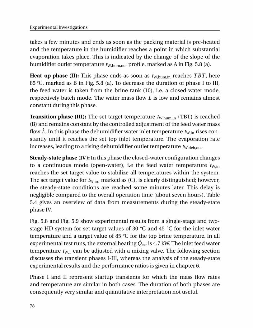
Experimental Investigations
takes a few minutes and ends as soon as the packing material is pre-heatedand the temperature in the humidifier reaches a point in which substantialevaporation takes place. This is indicated by the change of the slope of thehumidifier outlet temperature tW,hum,out profile, marked as A in Fig. 5.8 (a).
Heat-up phase (II): This phase ends as soon as tW,hum,in reaches T BT , here85 °C, marked as B in Fig. 5.8 (a). To decrease the duration of phase I to III,the feed water is taken from the brine tank (10), i.e. a closed-water mode,respectively batch mode. The water mass flow L is low and remains almostconstant during this phase.
Transition phase (III): The set target temperature tW,hum,in (TBT) is reached(B) and remains constant by the controlled adjustment of the feed water massflow L. In this phase the dehumidifier water inlet temperature tW,in rises con-stantly until it reaches the set top inlet temperature. The evaporation rateincreases, leading to a rising dehumidifier outlet temperature tW,deh,out.
Steady-state phase (IV): In this phase the closed-water configuration changesto a continuous mode (open-water), i.e the feed water temperature tW,in
reaches the set target value to stabilize all temperatures within the system.The set target value for tW,in, marked as (C), is clearly distinguished; however,the steady-state conditions are reached some minutes later. This delay isnegligible compared to the overall operation time (about seven hours). Table5.4 gives an overview of data from measurements during the steady-statephase IV.
Fig. 5.8 and Fig. 5.9 show experimental results from a single-stage and two-stage HD system for set target values of 30 °C and 45 °C for the inlet watertemperature and a target value of 85 °C for the top brine temperature. In allexperimental test runs, the external heating Qext is 4.7 kW. The inlet feed watertemperature tW,1 can be adjusted with a mixing valve. The following sectiondiscusses the transient phases I-III, whereas the analysis of the steady-stateexperimental results and the performance ratios is given in chapter 6.
Phase I and II represent startup transients for which the mass flow ratesand temperature are similar in both cases. The duration of both phases areconsequently very similar and quantitative interpretation not useful.
78
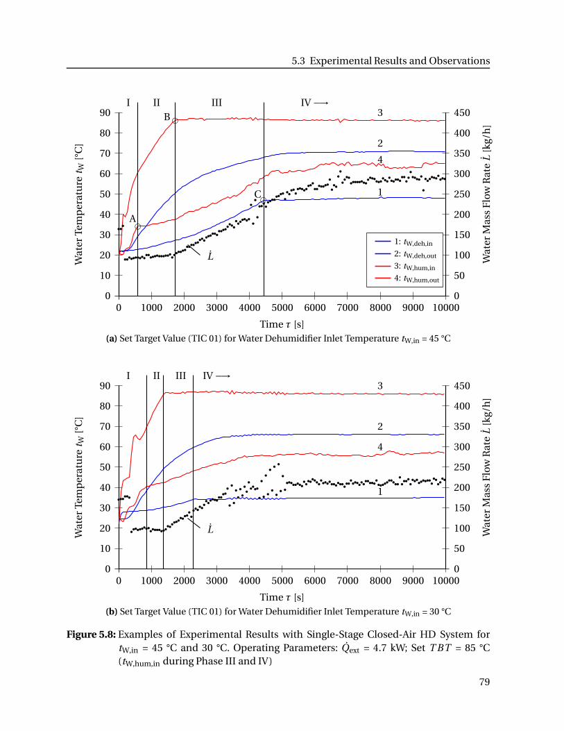
5.3 Experimental Results and Observations
0
10
20
30
40
50
60
70
80
90
0 1000 2000 3000 4000 5000 6000 7000 8000 9000 10000
Time τ [s]
Wat
erTe
mp
erat
ure
t W[°
C]
❡A
❡B
❡C
3
2
4
1
L
I II III IV −→
Wat
erM
ass
Flow
Rat
eL
[kg/
h]
0
50
100
150
200
250
300
350
400
450
1: tW,deh,in
2: tW,deh,out
3: tW,hum,in
4: tW,hum,out
(a) Set Target Value (TIC 01) for Water Dehumidifier Inlet Temperature tW,in = 45 °C
0
10
20
30
40
50
60
70
80
90
0 1000 2000 3000 4000 5000 6000 7000 8000 9000 10000
Time τ [s]
Wat
erTe
mp
erat
ure
t W[°
C]
3
2
4
1
L
I II III IV −→
Wat
erM
ass
Flow
Rat
eL
[kg/
h]
0
50
100
150
200
250
300
350
400
450
(b) Set Target Value (TIC 01) for Water Dehumidifier Inlet Temperature tW,in = 30 °C
Figure 5.8: Examples of Experimental Results with Single-Stage Closed-Air HD System fortW,in = 45 °C and 30 °C. Operating Parameters: Qext = 4.7 kW; Set T BT = 85 °C(tW,hum,in during Phase III and IV)
79
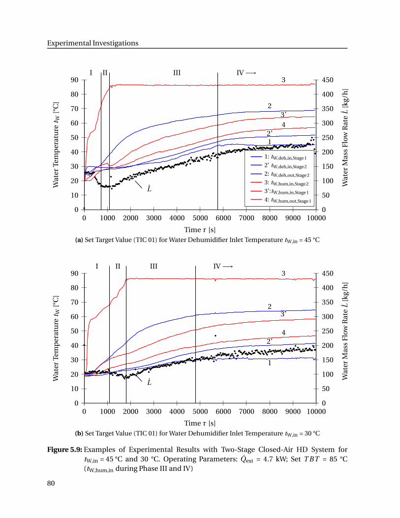
Experimental Investigations
0
10
20
30
40
50
60
70
80
90
0 1000 2000 3000 4000 5000 6000 7000 8000 9000 10000
Time τ [s]
Wat
erTe
mp
erat
ure
t W[°
C]
3
23’
2’4
1
L
I II III IV −→
Wat
erM
ass
Flow
Rat
eL
[kg/
h]
0
50
100
150
200
250
300
350
400
450
1: tW,deh,in,Stage1
2’ tW,deh,in,Stage2
2: tW,deh,out,Stage2
3: tW,hum,in,Stage2
3’:tW,hum,in,Stage1
4: tW,hum,out,Stage1
(a) Set Target Value (TIC 01) for Water Dehumidifier Inlet Temperature tW,in = 45 °C
0
10
20
30
40
50
60
70
80
90
0 1000 2000 3000 4000 5000 6000 7000 8000 9000 10000
Time τ [s]
Wat
erTe
mp
erat
ure
t W[°
C]
3
23’
42’
1
L
I II III IV −→
Wat
erM
ass
Flow
Rat
eL
[kg/
h]
0
50
100
150
200
250
300
350
400
450
(b) Set Target Value (TIC 01) for Water Dehumidifier Inlet Temperature tW,in = 30 °C
Figure 5.9: Examples of Experimental Results with Two-Stage Closed-Air HD System fortW,in = 45 °C and 30 °C. Operating Parameters: Qext = 4.7 kW; Set T BT = 85 °C(tW,hum,in during Phase III and IV)
80
5.3 Experimental Results and Observations
0
2
4
6
8
10
12
14
0 1000 2000 3000 4000 5000 6000 7000 8000 9000 10000
Time τ [s]
Co
nd
ensa
teM
ass
Flow
MC
on
d[k
g/h
]
Single-Stage, tW,in = 30 °C
Two-Stage, tW,in = 30 °CSingle-Stage, tW,in = 45 °C
Two-Stage, tW,in = 45 °C
Figure 5.10: Condensate Mass Flow MCond of Single-Stage and Two-Stage HD Setup. TotalExperimental Duration: 30,000 s
For the single-stage HD setup (Fig. 5.8) the duration of the transition phaseIII is shorter for lower feed water inlet temperatures tW,in due to the lowerfeed water mass flow rate L. This lower flow rate results from the higher watertemperature difference between dehumidifier inlet and outlet and constantexternal heat input Qext. The time for the transient phases can be furtherreduced by improving the system insulation and by recirculating hot brineproduced during the previous day. Experimental results for a two-stage HDsetup are shown in Fig. 5.9. The duration of the transient phase is also reducedwith lower water inlet temperature tW,in.
The condensate mass flow rate MCond is indicated in Fig. 5.10 for the abovementioned cases. It is relatively stable or even declines for the combinationof increasing water inlet temperature tW,1 and increasing feed water massflow rate L. The condensate mass flow rate MCond is calculated with thetemperature difference ∆t12 as per Eq. (4.21). It appears that the single stageconfiguration at lower inlet temperature achieves the highest condensatemass flow in initial phases. During the steady-state phase the condensatemass flow rates are similar for the single-stage configurations. The two-stageconfigurations show significant differences which are discussed in chapter 6.
81

Experimental Investigations
5.3.3 Results from Experiments Steady-State Phase
The following experimental data sets in Tab. 5.4 represent data obtainedfor both single-stage and two-stage configurations with natural convectionduring the steady-state phase IV. The data show average values of at leastfive measurement test runs for each test setup. The target value for the feedwater inlet temperature tW,in is set as a constant value for each test run. It wasexpected that increasing this parameter had a positive effect on the systemperformance.
Table 5.4: Overview Measurement Data of Experiments with Single-Stage (Numbers 1 – 6) andTwo-Stage HD System (Numbers 7 – 12)
tW,in tW,deh,out tW,hum,in tW,hum,out tA,deh,in L MCond Qext PR
No. °C °C °C °C °C kg/h kg/h kW -
Sin
gle-
Stag
e
1 26.6 63.8 86.4 48.4 68.1 181.9 10.3 4.7 1.39
2 30.5 65.1 86.2 53.7 69.3 191.3 10.3 4.7 1.41
3 35.0 66.1 85.9 57.2 70.2 209.8 10.3 4.7 1.38
4 39.3 67.7 86.0 59.5 71.7 230.1 10.1 4.7 1.33
5 43.4 69.4 86.0 62.7 73.6 254.3 10.4 4.7 1.36
6 47.9 70.8 85.9 65.7 75.0 283.7 9.6 4.7 1.24
Two
-Sta
ge
7 25.5 62.0 86.2 42.6 78.9 163.1 10.4 4.7 1.47
8 30.9 64.7 86.1 47.6 80.3 183.5 10.8 4.7 1.52
9 36.1 66.3 86.1 51.1 81.0 199.3 11.2 4.7 1.58
10 40.4 67.5 86.1 53.5 81.4 210.2 10.8 4.7 1.54
11 45.4 69.3 86.3 57.6 82.1 231.6 10.7 4.7 1.51
12 50.3 71.3 86.3 62.8 83.0 267.8 12.3 4.7 1.71
The displayed data are average values of experiments with the same targetvalue for tW,in, T BT and Qext during steady-state conditions. The determinedP R values are based on the condensate mass flow rate Mcond. The P R valuesdon’t show a clear tendency with increasing water inlet temperature tW,in re-spectively with increasing feed water mass flow L. As mentioned in chapter5.2.1 the measurement error for condensate mass flow rates Mcond is high. Thenext chapter introduces an adapted performance ratio which is dependent ontemperature measurements and consequently applicable for a more preciseanalysis.
82
6 Analysis
This chapter analyzes the experimental data provided in chapter 5. An advan-tageous definition for the performance ratio is introduced to evaluate andanalyse experimental results with adequate precision. Applying the conven-tional definition of the performance ratio is not recommended as it may leadto misinterpretation due to the high inaccuracy for the studied small system.The experimental data are used as input values for the 1-D numerical simula-tion to visualize heat and mass transfer relations described in chapter 4.3.
On this basis the limitations of the studied HD system with natural convec-tion are identified. Suggestions to overcome these limitations are outlined inchapter 7.
6.1 Introduction Adapted Performance Ratio P RHD
The conventional performance ratio P R, as defined in Eq. (3.2) is commonlyused to determine the efficiency of a HD system or the Gained Output RatioGOR which is further described in Appendix A. However, determination of thecondensate mass flow MCond is associated with high measurement errors duethe small quantity per time interval for systems, which have a low condensatemass flow and/or a high liquid hold-up from droplets adhering to the heatexchanger surface of the dehumidifier.
Because of these limitations, an advantagous performance ratio P RHD isrecommended to continuously determine the efficiency during operationwith appropriate precision.
P RHD is adapted from the conventional performance ratio P R to determinethe multi-effectiveness of thermal desalination plants. It is particularly usefulfor small-scale systems and as optimization parameter during the operation.
The internally transferred heat flow Hint is described in the next section as it isconsidered for the derivation of the definition of P RHD.
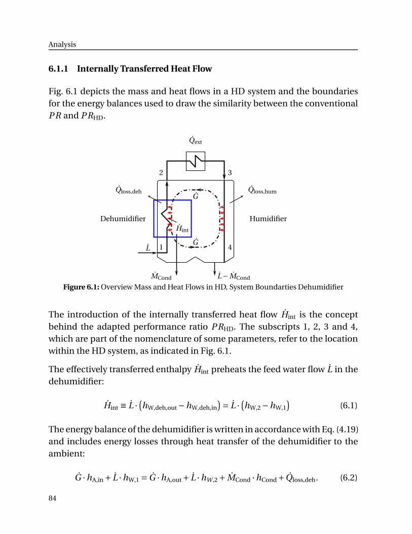
Analysis
6.1.1 Internally Transferred Heat Flow
Fig. 6.1 depicts the mass and heat flows in a HD system and the boundariesfor the energy balances used to draw the similarity between the conventionalP R and P RHD.
Dehumidifier Humidifier
G
G
L 1
2 3
4
L − MCond
Qext
Qloss,deh Qloss,hum
MCond
Hint
Figure 6.1: Overview Mass and Heat Flows in HD, System Boundarties Dehumidifier
The introduction of the internally transferred heat flow Hint is the conceptbehind the adapted performance ratio P RHD. The subscripts 1, 2, 3 and 4,which are part of the nomenclature of some parameters, refer to the locationwithin the HD system, as indicated in Fig. 6.1.
The effectively transferred enthalpy Hint preheats the feed water flow L in thedehumidifier:
Hint ≡ L ·(
hW,deh,out −hW,deh,in
)
= L ·(
hW,2 −hW,1
)
(6.1)
The energy balance of the dehumidifier is written in accordance with Eq. (4.19)and includes energy losses through heat transfer of the dehumidifier to theambient:
G ·hA,in+ L ·hW,1 = G ·hA,out+ L ·hW,2 + MCond ·hCond+Qloss,deh. (6.2)
84
6.1 Adapted Performance Ratio PRHD
6.1.2 Definition Adapted Performance Ratio P RHD
The here proposed adapted performance ratio P RHD relates the internallyregained energy flow rate Hint utilized for preheating the feed water in thedehumidifier to the external energy flow Qext:
P RHD ≡Hint
Qext. (6.3)
The multi-effect in HD is not created from multiple condensation processes(as it is applied for example in large-scale MED systems) but from the reduc-tion of the external energy requirements.
For constant feed water mass flow rate L, P RHD can be approximated as theratio of the temperature difference tW,2 − tW,1 of feed water between inletand outlet in the dehumidifier and the temperature difference tW,3 − tW,2
of feed water between inlet and outlet in the external heater. This neglectssmall deviations of the specific heat cp,W of the feed water flow. Therefore thecorrelation corresponds to Eq. (4.21) and Eq. (3.2):
P RHD =tW,2 − tW,1
tW,3 − tW,2=
∆t12
∆t23. (6.4)
This performance ratio only requires the measurement of three temperatureswithin the liquid water flow. Hodges et al. [46, p. 91] define this ratio asthe ‘number of effects’ of the HD system. Meinel et al. [67, p. 556] expressthe grade of multi-effectiveness1 for Hodges’ HD system as the ratio of thetemperature differences ∆t13/∆t23. This definition results in a dimensionlessnumber, which is (P RHD +1).
For the calculation of P RHD it is sufficient to determine the water temperaturestW,1, tW,2 and tW,3, as outlined in Eq. (6.4). As these temperatures can bemeasured with high accuracy, P RHD can be determined with a relative errorof less than 2%.
1 Traditional solar stills don’t recover the heat of condensation to preheat the feed water, resulting in a PRHD = 0,which strongly deviates from PR = mDist ·∆hv/Qin.
85
Analysis
P RHD offers a variety of advantages, especially for small-scale HD systems:
1. P RHD requires only temperatures of the feed water within the system,which can be measured more accurately, with higher reproducibilityand faster compared to measuring small water mass flow rates for thecalculation of P R.
2. P RHD can be constantly determined during the operation, whereasthe conventional performance ratio P R requires the measurement ofcondensate within a certain period of time.
3. P RHD uses the prevailing temperature differences, which correspond tothe transferred heat, whereas P R normalizes ∆hv to 1000 BTU/lb.
4. The condensate mass flow rate MCond can be constantly approxima-ted during steady-state conditions with known external heat input:MCond ≈P RHD ·Qext/∆hv, as per Eq. (4.21) and Eq. (6.4). The heat ofcondensation ∆hv has to be chosen for a mean interface temperature.
6.1.3 Comparison P R and P RHD
Inserting the correlation for the enthalpy of humid air according to Eq. (4.1)(for ideal gases) into Eq. (6.2) follows:
G ·[
cp,G · tA,in+XA,in ·(
cp,V · tA,in+∆hv,0
)]
+ L ·hW,1 = L ·hW,2+ MCond ·hCond
+G ·[
cp,G · tA,out+XA,out ·(
cp,V · tA,out+∆hv,0
)]
+Qloss,deh. (6.5)
This leads to an equation for Hint expressed as the energy transport of thehumid air in the dehumidifier, which is applied for the comparison with theconventional performance ratio:
Hint = G · cp,G ·(
tA,in − tA,out
)
+G ·[
XA,in · cp,V · tA,in−XA,out · cp,V · tA,out
]
+ G ·(
XA,in−XA,out
)
·∆hv,0 − MCond ·hCond−Qloss,deh. (6.6)
This formula is translated into an equation for P RHD according to Eq. (6.4).Eq. (6.6) is divided by the external heat input Qext. The definition of P R as per
86
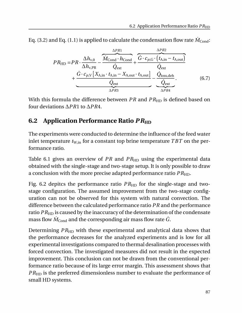
6.2 Application Performance Ratio PRHD
Eq. (3.2) and Eq. (1.1) is applied to calculate the condensation flow rate MCond:
P RHD =P R ·∆hv,0
∆hv,PR−
∆PR1︷ ︸︸ ︷
MCond ·hCond
Qext+
∆PR2︷ ︸︸ ︷
G · cp,G ·(
tA,in− tA,out
)
Qext
+G · cp,V
[
XA,in · tA,in−XA,out · tA,out
]
Qext︸ ︷︷ ︸
∆PR3
−Qloss,deh
Qext︸ ︷︷ ︸
∆PR4
. (6.7)
With this formula the difference between P R and P RHD is defined based onfour deviations ∆P R1 to ∆P R4.
6.2 Application Performance Ratio P RHD
The experiments were conducted to determine the influence of the feed waterinlet temperature tW,in for a constant top brine temperature T BT on the per-formance ratio.
Table 6.1 gives an overview of P R and P RHD using the experimental dataobtained with the single-stage and two-stage setup. It is only possible to drawa conclusion with the more precise adapted performance ratio P RHD.
Fig. 6.2 depitcs the performance ratio P RHD for the single-stage and two-stage configuration. The assumed improvement from the two-stage config-uration can not be observed for this system with natural convection. Thedifference between the calculated performance ratio P R and the performanceratio P RHD is caused by the inaccuracy of the determination of the condensatemass flow MCond and the corresponding air mass flow rate G .
Determining P RHD with these experimental and analytical data shows thatthe performance decreases for the analyzed experiments and is low for allexperimental investigations compared to thermal desalination processes withforced convection. The investigated measures did not result in the expectedimprovement. This conclusion can not be drawn from the conventional per-formance ratio because of its large error margin. This assessment shows thatP RHD is the preferred dimensionless number to evaluate the performance ofsmall HD systems.
87
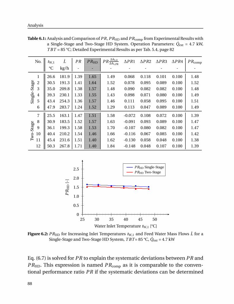
Analysis
Table 6.1: Analysis and Comparison of PR , PRHD and PRcomp from Experimental Results witha Single-Stage and Two-Stage HD System. Operation Parameters: Qext = 4.7 kW,T BT = 85 °C; Detailed Experimental Results as per Tab. 5.4, page 82
No. tW,1 L PR PRHD PR ∆hv,0∆hv,PR
∆PR1 ∆PR2 ∆PR3 ∆PR4 PRcomp
°C kg/h - - - - - - - -
Sin
gle-
Stag
e
1 26.6 181.9 1.39 1.65 1.49 0.068 0.118 0.101 0.100 1.48
2 30.5 191.3 1.41 1.64 1.52 0.078 0.095 0.089 0.100 1.52
3 35.0 209.8 1.38 1.57 1.48 0.090 0.082 0.082 0.100 1.48
4 39.3 230.1 1.33 1.55 1.43 0.098 0.071 0.080 0.100 1.49
5 43.4 254.3 1.36 1.57 1.46 0.111 0.058 0.095 0.100 1.51
6 47.9 283.7 1.24 1.52 1.29 0.113 0.047 0.089 0.100 1.49
Two
-Sta
ge
7 25.5 163.1 1.47 1.51 1.58 -0.072 0.108 0.072 0.100 1.39
8 30.9 183.5 1.52 1.57 1.63 -0.091 0.093 0.089 0.100 1.47
9 36.1 199.3 1.58 1.53 1.70 -0.107 0.080 0.082 0.100 1.47
10 40.4 210.2 1.54 1.46 1.66 -0.116 0.067 0.085 0.100 1.42
11 45.4 231.6 1.51 1.40 1.62 -0.130 0.058 0.048 0.100 1.38
12 50.3 267.8 1.71 1.40 1.84 -0.148 0.048 0.107 0.100 1.39
0
0.5
1.0
1.5
2.0
2.5
25 30 35 40 45 50
Water Inlet Temperature tW,1 [°C]
PR
HD
[-]
PRHD Single-StagePRHD Two-Stage
Figure 6.2: PRHD for Increasing Inlet Temperatures tW,1 and Feed Water Mass Flows L for aSingle-Stage and Two-Stage HD System, T BT = 85 °C, Qext = 4.7 kW
Eq. (6.7) is solved for P R to explain the systematic deviations between P R andP RHD. This expression is named P Rcomp as it is comparable to the conven-tional performance ratio P R if the systematic deviations can be determined
88
6.3 Application Operating Lines
accurately:
P Rcomp = (P RHD+∆P R1−∆P R2−∆P R3+∆P R4) ·∆hv,PR
∆hv,0. (6.8)
Since the deviations are determined from measurement data with relativehigh uncertainties (tA,in) and assumptions (thermal losses), P Rcomp can onlybe used as an indication to show that the deviations are small or partiallycompensate each other. The thermal losses of the dehumidifier ∆P R4 areaccounted for as 10% of the external energy.
Obviously the performance would increase by enlarging the available heat andmass transfer surfaces but these efforts are limited by the driving potentialsanalysed and visualized in the following section. Combining Eq. (4.21) andEq. (4.22) proves that for a given external heat input Qext the maximum con-densate mass flow MCond can be achieved if the performance ratio P RHD ismaximised.
6.3 Application Operating Lines
6.3.1 Generation of Operating Lines
Operating lines represent a simplified visualization of the conditions withinthe humidifier and dehumidifier. The principles of operating lines are de-scribed in chapter 4.3.3. Each point on the operating line marks the specificenthalpy hA of bulk humid air flow as a function of the bulk water flowtemperature at a column height. The diagrams include the saturation lineof humid air whereby the x-axis is interpreted as the temperature of saturatedhumid air.
These values indicate the conditions of the saturated humid air at the interfacebetween air and water in the humidifier and dehumidifier. Heat and masstransfer processes and the determination of the interface temperature areexplained in chapter 4.3.2. The visualization of the driving potential with atie line is detailed in chapter 4.5.1.
The operating lines for humidification and dehumidification are determined
89
Analysis
from the energy and mass balances described in chapter 4.3.1 (humidifier)and chapter 4.4.1 (dehumidifier). The introduced simplifications lead to equalequations for the slope of the operating lines, refer Eq. (4.18) and Eq. (4.20).
The slope of the operating line dhA/dtW ≈ L/G · cp,W depends on the ratio ofthe flow rate L of water and G of air. The water flow rate L is adjustable. Ex-perimental values were used as input data for the 1-D simulation to calculatethe air mass flow rate and to create the operating lines.
Fig. 6.3 shows an example of the operating lines for a single-stage and two-stage HD configuration. The enthalpy of humid air hA at the top in (2) and (3)and the bottom (1) and (4) does not change as the air is only transferred fromone column to the other.
The temperature tW,in of the feed water flow is depicted in point (1). Theinfluence of this temperature is investigated in the following subsection forthe studied single-stage and two-stage HD systems. The transferred enthalpyflow Hint, cp. Eq. (4.21), preheats the feed water in the dehumidifier resultingin a proportional temperature difference ∆t12 of the feed water, point (2).
Fig. 6.3b depicts the operating lines for each stage of the two-stage HD con-figuration. Stage 1 is indicated as (1) to (2’) and Stage 2 as (3’) and (4). Thediagram also indicates the deviation of the operating lines to the theoreticalslope of the operating line of the dehumidifier, i.e. parallel to the operatingline of the dehumidifier. The water temperatures 3’a and 4a deviate from themeasure temperatures 3’ and 4. These deviations are due to the inaccuratemeasurement of the water temperatures and heat losses in the humidifier.
The brine outlet temperature tW,4 is not required to determine P RHD. For thedetermination of the specific enthalpy hA of humid air at position 1 and 4 (y-axis), the mean temperatures measured at the exit of the dehumidifier andentry of the humidifier are used.
6.3.2 Operating Lines for Single-Stage and Two-Stage HD
Fig. 6.4 and Fig. 6.5 show the operating lines for the single-stage and two-stageexperiments for various feed water inlet temperatures. The operating lines are
90
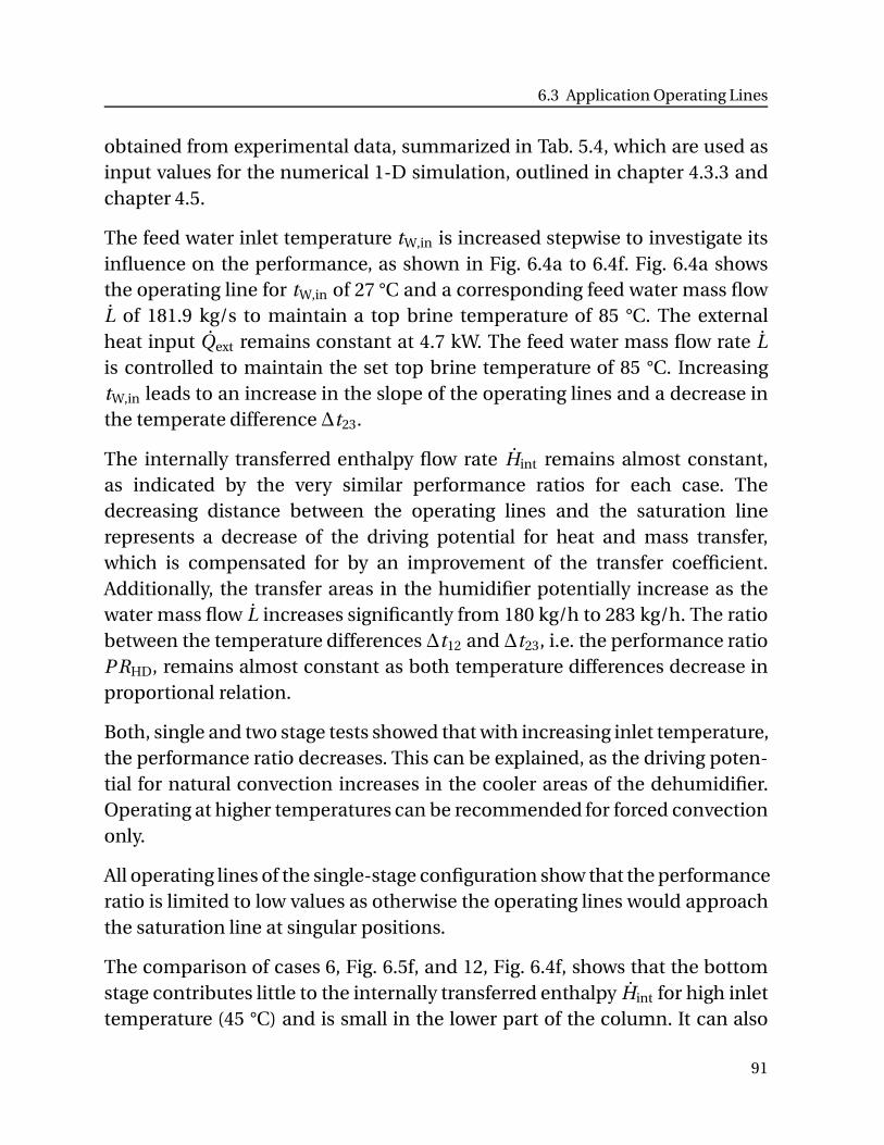
6.3 Application Operating Lines
obtained from experimental data, summarized in Tab. 5.4, which are used asinput values for the numerical 1-D simulation, outlined in chapter 4.3.3 andchapter 4.5.
The feed water inlet temperature tW,in is increased stepwise to investigate itsinfluence on the performance, as shown in Fig. 6.4a to 6.4f. Fig. 6.4a showsthe operating line for tW,in of 27 °C and a corresponding feed water mass flowL of 181.9 kg/s to maintain a top brine temperature of 85 °C. The externalheat input Qext remains constant at 4.7 kW. The feed water mass flow rate Lis controlled to maintain the set top brine temperature of 85 °C. IncreasingtW,in leads to an increase in the slope of the operating lines and a decrease inthe temperate difference ∆t23.
The internally transferred enthalpy flow rate Hint remains almost constant,as indicated by the very similar performance ratios for each case. Thedecreasing distance between the operating lines and the saturation linerepresents a decrease of the driving potential for heat and mass transfer,which is compensated for by an improvement of the transfer coefficient.Additionally, the transfer areas in the humidifier potentially increase as thewater mass flow L increases significantly from 180 kg/h to 283 kg/h. The ratiobetween the temperature differences ∆t12 and ∆t23, i.e. the performance ratioP RHD, remains almost constant as both temperature differences decrease inproportional relation.
Both, single and two stage tests showed that with increasing inlet temperature,the performance ratio decreases. This can be explained, as the driving poten-tial for natural convection increases in the cooler areas of the dehumidifier.Operating at higher temperatures can be recommended for forced convectiononly.
All operating lines of the single-stage configuration show that the performanceratio is limited to low values as otherwise the operating lines would approachthe saturation line at singular positions.
The comparison of cases 6, Fig. 6.5f, and 12, Fig. 6.4f, shows that the bottomstage contributes little to the internally transferred enthalpy Hint for high inlettemperature (45 °C) and is small in the lower part of the column. It can also
91
Analysis
be observed that for higher temperatures the upper part is more effectivebut the overall performance ratio is smaller because the smaller temperaturedifferences reduce the natural convection flow.
In a multi-stage configuration, the operating lines could be adjusted to thesaturation line if the air flow is adjusted (forced convection). All figures showthat the ability to adjust the slope along the saturation line is desirable. HDsetups with natural convection offer only limited opportunities compared toforced convection.
92
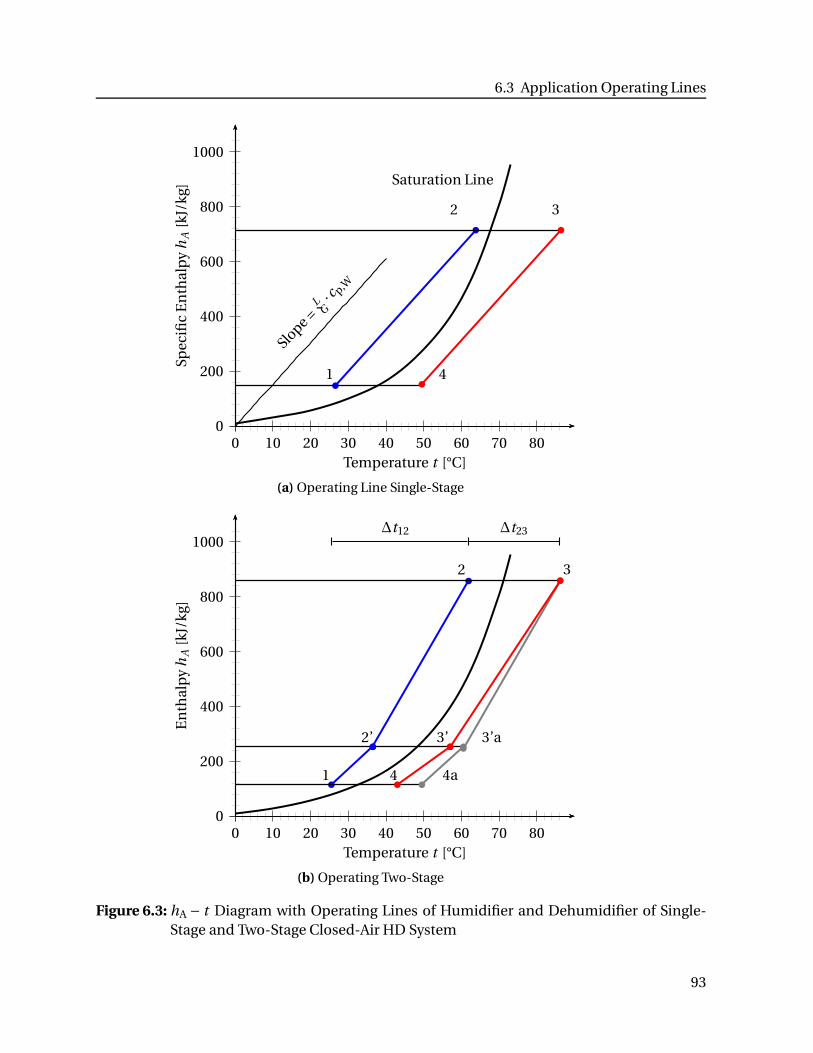
6.3 Application Operating Lines
0
200
400
600
800
1000
0 10 20 30 40 50 60 70 80Temperature t [°C]
Spec
ific
En
thal
py
hA
[kJ/
kg] Saturation Line
Slope =
LG·c p,W
1
2 3
4
(a) Operating Line Single-Stage
0
200
400
600
800
1000
0 10 20 30 40 50 60 70 80Temperature t [°C]
En
thal
py
hA
[kJ/
kg]
1
2’
2 3
3’ 3’a
4 4a
∆t12 ∆t23
(b) Operating Two-Stage
Figure 6.3: hA − t Diagram with Operating Lines of Humidifier and Dehumidifier of Single-Stage and Two-Stage Closed-Air HD System
93
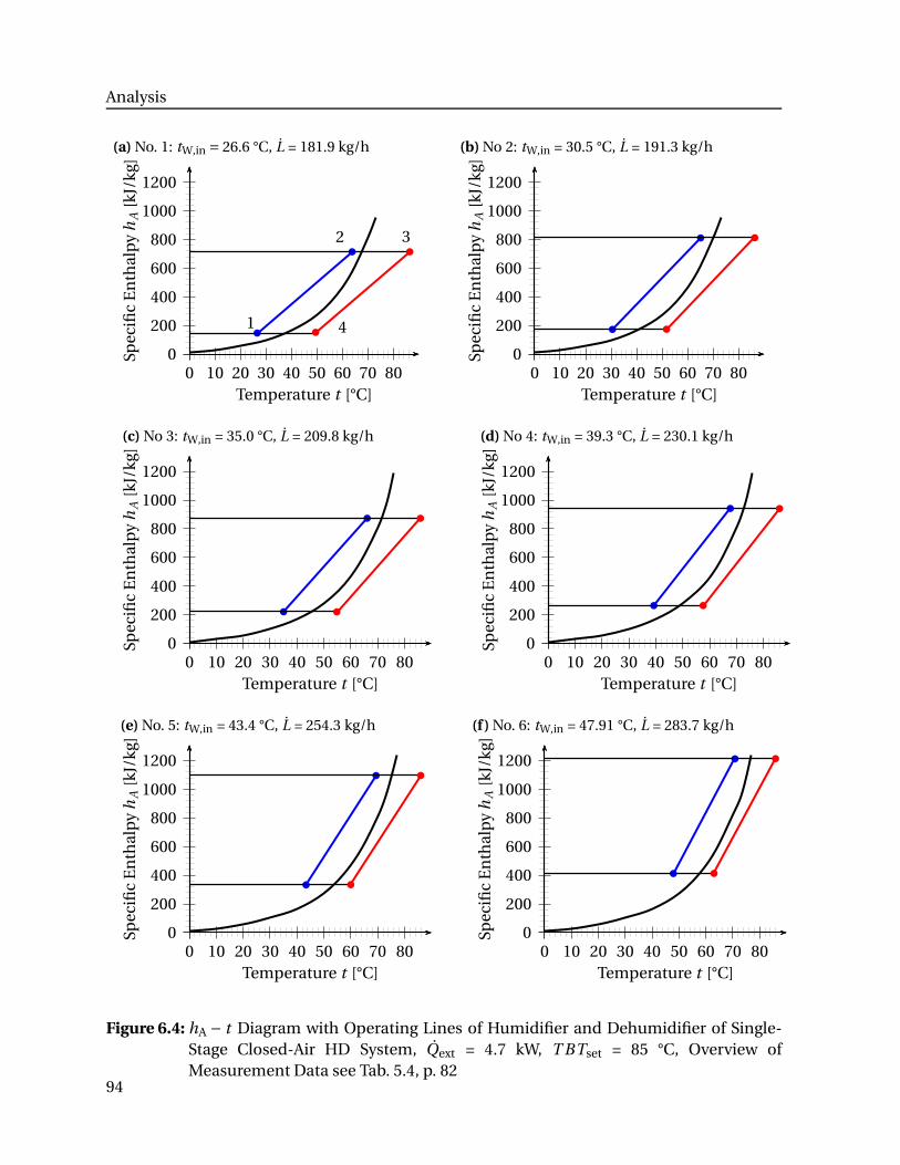
Analysis
(a) No. 1: tW,in = 26.6 °C, L = 181.9 kg/h
0
200
400
600
800
1000
1200
0 10 20 30 40 50 60 70 80Temperature t [°C]
Spec
ific
En
thal
py
hA
[kJ/
kg]
1
2 3
4
(b) No 2: tW,in = 30.5 °C, L = 191.3 kg/h
0
200
400
600
800
1000
1200
0 10 20 30 40 50 60 70 80Temperature t [°C]
Spec
ific
En
thal
py
hA
[kJ/
kg]
(c) No 3: tW,in = 35.0 °C, L = 209.8 kg/h
0
200
400
600
800
1000
1200
0 10 20 30 40 50 60 70 80Temperature t [°C]
Spec
ific
En
thal
py
hA
[kJ/
kg]
(d) No 4: tW,in = 39.3 °C, L = 230.1 kg/h
0
200
400
600
800
1000
1200
0 10 20 30 40 50 60 70 80Temperature t [°C]
Spec
ific
En
thal
py
hA
[kJ/
kg]
(e) No. 5: tW,in = 43.4 °C, L = 254.3 kg/h
0
200
400
600
800
1000
1200
0 10 20 30 40 50 60 70 80Temperature t [°C]
Spec
ific
En
thal
py
hA
[kJ/
kg]
(f ) No. 6: tW,in = 47.91 °C, L = 283.7 kg/h
0
200
400
600
800
1000
1200
0 10 20 30 40 50 60 70 80Temperature t [°C]
Spec
ific
En
thal
py
hA
[kJ/
kg]
Figure 6.4: hA − t Diagram with Operating Lines of Humidifier and Dehumidifier of Single-Stage Closed-Air HD System, Qext = 4.7 kW, T BTset = 85 °C, Overview ofMeasurement Data see Tab. 5.4, p. 82
94
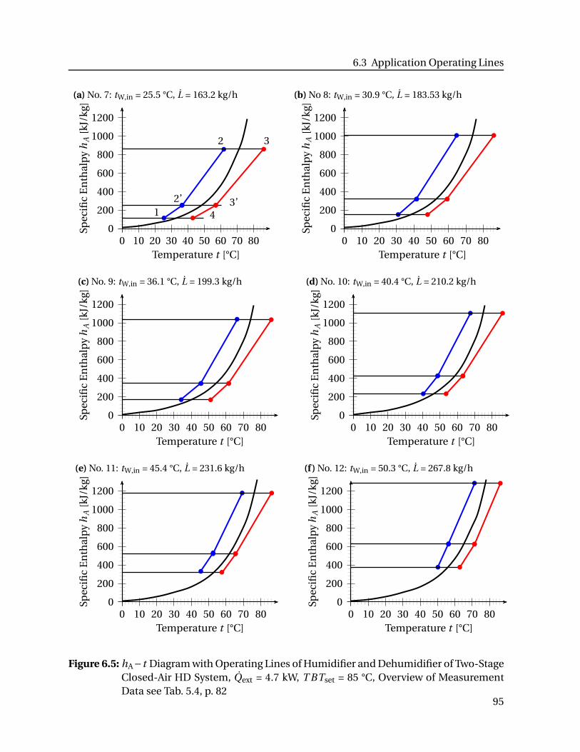
6.3 Application Operating Lines
(a) No. 7: tW,in = 25.5 °C, L = 163.2 kg/h
0
200
400
600
800
1000
1200
0 10 20 30 40 50 60 70 80Temperature t [°C]
Spec
ific
En
thal
py
hA
[kJ/
kg]
12’
2 3
3’4
(b) No 8: tW,in = 30.9 °C, L = 183.53 kg/h
0
200
400
600
800
1000
1200
0 10 20 30 40 50 60 70 80Temperature t [°C]
Spec
ific
En
thal
py
hA
[kJ/
kg]
(c) No. 9: tW,in = 36.1 °C, L = 199.3 kg/h
0
200
400
600
800
1000
1200
0 10 20 30 40 50 60 70 80Temperature t [°C]
Spec
ific
En
thal
py
hA
[kJ/
kg]
(d) No. 10: tW,in = 40.4 °C, L = 210.2 kg/h
0
200
400
600
800
1000
1200
0 10 20 30 40 50 60 70 80Temperature t [°C]
Spec
ific
En
thal
py
hA
[kJ/
kg]
(e) No. 11: tW,in = 45.4 °C, L = 231.6 kg/h
0
200
400
600
800
1000
1200
0 10 20 30 40 50 60 70 80Temperature t [°C]
Spec
ific
En
thal
py
hA
[kJ/
kg]
(f ) No. 12: tW,in = 50.3 °C, L = 267.8 kg/h
0
200
400
600
800
1000
1200
0 10 20 30 40 50 60 70 80Temperature t [°C]
Spec
ific
En
thal
py
hA
[kJ/
kg]
Figure 6.5: hA−t Diagram with Operating Lines of Humidifier and Dehumidifier of Two-StageClosed-Air HD System, Qext = 4.7 kW, T BTset = 85 °C, Overview of MeasurementData see Tab. 5.4, p. 82
95
Analysis
6.3.3 Number of Transfer Units and Height of one Transfer Unit
The 1-D numerical simulation tool is used for the dimensioning of thehumidifier and dehumidifier columns. A commonly used approach to de-termine the height of a column is defined in chapter 4.5.2.
The number of transfer units describes the ‘difficulty’ of the heat and masstransfer process [69]. Heat and mass transfer conditions can be visualized inthe known manner by applying the graphical concept of the operating linesand further analyzing the number of transfer units NTU and the height ofone transfer unit HTU as described in chapter 4.5.1.
The accuracy of the measurement values of the feed water temperatures tW,1,tW,2 and tW,3 (x-coordinate) is high as the water temperature is obtained frommeasurements within tubes. In contrast, the accuracy of the value for thebrine temperature tW,4 is reduced as the measurements involve a thermo-couple overflowed with brine. Time variations during the draining can affectthe measurement accuracy. These uncertainties during the determination oftW,4 are reflected by indicating the operating line of the humidifier as a dashedline.
The temperature difference tW,4 − tW,1 is approximated with the temperaturedifference tW,3−tW,2. This follows from an energy balance on the overall systemwhereby the specific enthalpy of the condensation mass flow is deemed to besimilar to the specific enthalpy of the brine water flow and the specific heatcapacities are the same.
An increasing NTU corresponds to higher demands for the transport processas the driving potential decreases. The visualization of the heat and masstransfer processes with the operating lines, tie lines and consideration ofNTU and HTU show that the NTUs are not large because the operatinglines approach the saturation line. However, these low NTUs involve largetemperature differences ∆t23 leading to small performance ratios.
NTU increases extremely for conditions in which the transfer takes placeat a small driving potential that is created when the operating line becomestangent to the saturation line or both lines converge. The HTU increases
96
6.3 Application Operating Lines
for larger quantities of fluids to be separated (proportional to G) and forsmaller separation column efficiency, i.e. smaller transfer surface and smallertransport coefficients.
With graphic visualization of the operating lines it is possible to detect dis-advantageous transfer conditions in the humidifier and dehumidifier. Theapproach of the saturation line with the operating line can be avoided byadjusting the operational lines according to the temperature dependent slopeof the saturation line.
The slope of the operating line incorporates the mass flow G of dry air, whichis derived from the energy and mass balance of the condensate and thedifference of the absolute humidity ∆X . Consequently, the slope indicatesan average value of G that changes over height due to the cross flow createdby the removal of the separation wall between humidifier and dehumidifier.The intersection point of the operating line with the water temperature tW,2
results in the enthalpy hA,2 of humid air. The exact operating line would be(slightly) curved as the denominator of L/G changes over the column heightof humidifier and dehumidifier. Measurement of the feed water temperaturescan be done with a higher accuracy than air temperatures within the system.
As shown for a multi-stage HD in Fig. 6.5, the operating line is bent accordingto the number of stages. The produced condensate flow in the bottom stageis low because of the low absolute humidity in air in this temperature region.The flat slope of the operating line results from a higher air velocity.
The approach of the operating lines towards the saturation line can becounter-steered by reducing the temperature difference t12 and aimingsimultaneously to reduce the temperature difference t23 to achieve a highperformance ratio P RHD. This is easier to accomplish in lower temperatureregions (up to 50 °C) as the curvature of the saturation line is smaller than inthe higher temperature regions.
Tab. 6.2 indicates the slope L/G · cp,W, NTUG and HTUG for the each theexperimental data as shown in Tab. 5.4. It also includes the effectivelytransferred enthalpy flow rate Hint according Eq. (6.1). The enthalpy flow rateslightly decreases with increasing feed water inlet temperature tW,in for both
97
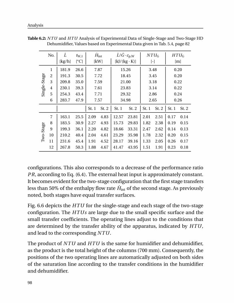
Analysis
Table 6.2: NTU and HTU Analysis of Experimental Data of Single-Stage and Two-Stage HDDehumidifier, Values based on Experimental Data given in Tab. 5.4, page 82
No. L tW,1 Hint L/G ·cp,W NTUG HTUG
[kg/h] [°C ] [kW] [kJ/(kg · K)] [-] [m]
Sin
gle-
Stag
e
1 181.9 26.6 7.87 15.26 3.48 0.20
2 191.3 30.5 7.72 18.45 3.45 0.20
3 209.8 35.0 7.59 21.00 3.18 0.22
4 230.1 39.3 7.61 23.83 3.14 0.22
5 254.3 43.4 7.71 29.32 2.86 0.24
6 283.7 47.9 7.57 34.98 2.65 0.26
St. 1 St. 2 St. 1 St. 2 St. 1 St. 2 St. 1 St. 2
Two
-Sta
ge
7 163.1 25.5 2.09 4.83 12.57 23.81 2.01 2.51 0.17 0.14
8 183.5 30.9 2.27 4.93 15.73 29.83 1.82 2.38 0.19 0.15
9 199.3 36.1 2.20 4.82 18.66 33.31 2.47 2.62 0.14 0.13
10 210.2 40.4 2.04 4.61 23.29 35.98 1.78 2.32 0.20 0.15
11 231.6 45.4 1.91 4.52 28.17 39.16 1.33 2.05 0.26 0.17
12 267.8 50.3 1.88 4.67 41.47 43.95 1.51 1.91 0.23 0.18
configurations. This also corresponds to a decrease of the performance ratioP R, according to Eq. (6.4). The external heat input is approximately constant.It becomes evident for the two-stage configuration that the first stage transfersless than 50% of the enthalpy flow rate Hint of the second stage. As previouslynoted, both stages have equal transfer surfaces.
Fig. 6.6 depicts the HTU for the single-stage and each stage of the two-stageconfiguration. The HTUs are large due to the small specific surface and thesmall transfer coefficients. The operating lines adjust to the conditions thatare determined by the transfer ability of the apparatus, indicated by HTU ,and lead to the corresponding NTU .
The product of NTU and HTU is the same for humidifier and dehumidifier,as the product is the total height of the columns (700 mm). Consequently, thepositions of the two operating lines are automatically adjusted on both sidesof the saturation line according to the transfer conditions in the humidifierand dehumidifier.
98
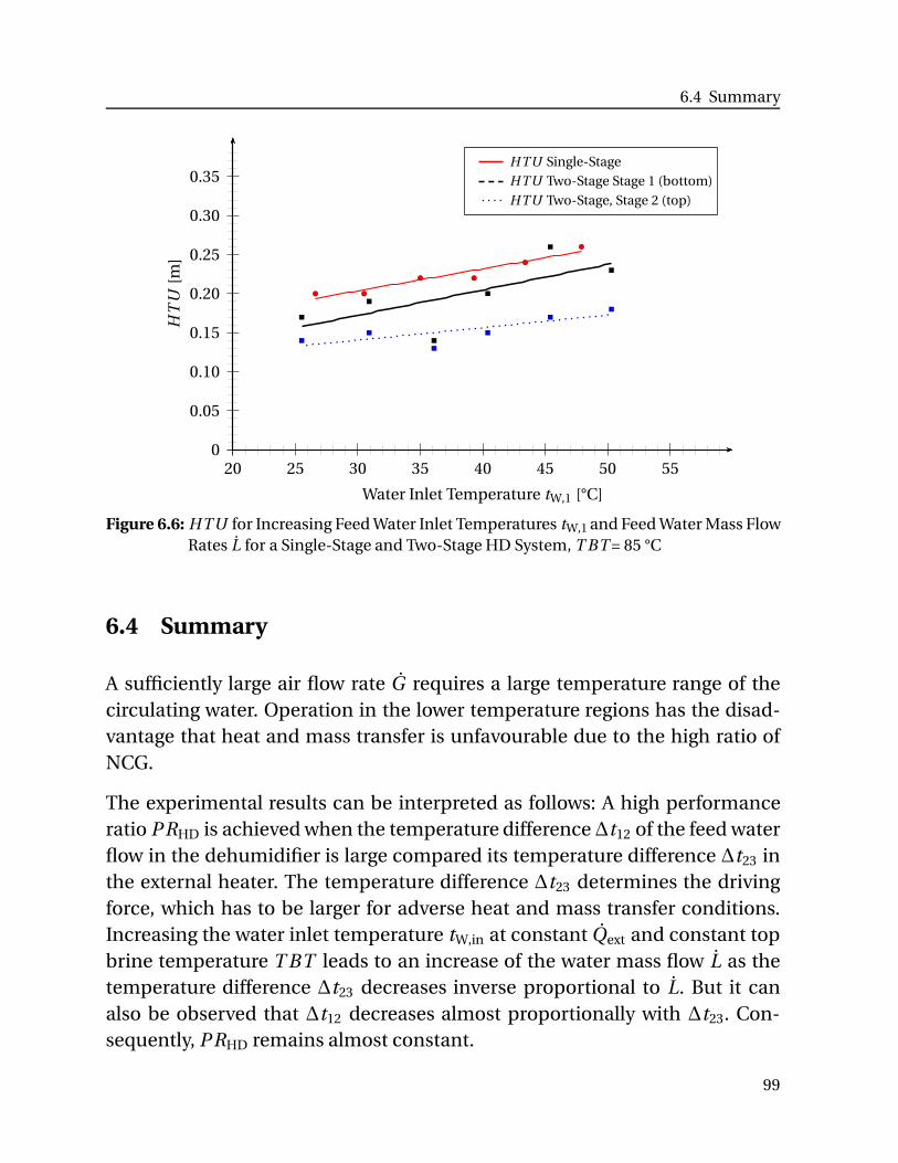
6.4 Summary
0
0.05
0.10
0.15
0.20
0.25
0.30
0.35
20 25 30 35 40 45 50 55
Water Inlet Temperature tW,1 [°C]
HT
U[m
]HTU Single-StageHTU Two-Stage Stage 1 (bottom)
HTU Two-Stage, Stage 2 (top)
Figure 6.6: HTU for Increasing Feed Water Inlet Temperatures tW,1 and Feed Water Mass FlowRates L for a Single-Stage and Two-Stage HD System, T BT = 85 °C
6.4 Summary
A sufficiently large air flow rate G requires a large temperature range of thecirculating water. Operation in the lower temperature regions has the disad-vantage that heat and mass transfer is unfavourable due to the high ratio ofNCG.
The experimental results can be interpreted as follows: A high performanceratio P RHD is achieved when the temperature difference ∆t12 of the feed waterflow in the dehumidifier is large compared its temperature difference ∆t23 inthe external heater. The temperature difference ∆t23 determines the drivingforce, which has to be larger for adverse heat and mass transfer conditions.Increasing the water inlet temperature tW,in at constant Qext and constant topbrine temperature T BT leads to an increase of the water mass flow L as thetemperature difference ∆t23 decreases inverse proportional to L. But it canalso be observed that ∆t12 decreases almost proportionally with ∆t23. Con-sequently, P RHD remains almost constant.
99
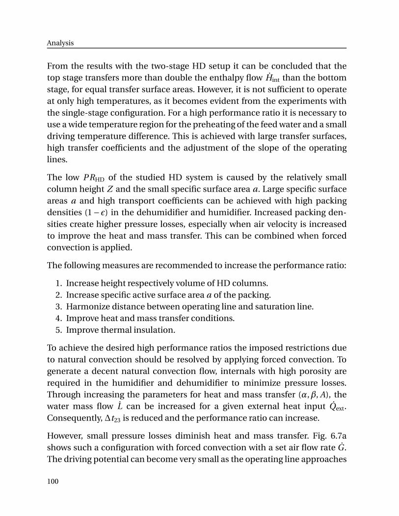
Analysis
From the results with the two-stage HD setup it can be concluded that thetop stage transfers more than double the enthalpy flow Hint than the bottomstage, for equal transfer surface areas. However, it is not sufficient to operateat only high temperatures, as it becomes evident from the experiments withthe single-stage configuration. For a high performance ratio it is necessary touse a wide temperature region for the preheating of the feed water and a smalldriving temperature difference. This is achieved with large transfer surfaces,high transfer coefficients and the adjustment of the slope of the operatinglines.
The low P RHD of the studied HD system is caused by the relatively smallcolumn height Z and the small specific surface area a. Large specific surfaceareas a and high transport coefficients can be achieved with high packingdensities (1− ϵ) in the dehumidifier and humidifier. Increased packing den-sities create higher pressure losses, especially when air velocity is increasedto improve the heat and mass transfer. This can be combined when forcedconvection is applied.
The following measures are recommended to increase the performance ratio:
1. Increase height respectively volume of HD columns.2. Increase specific active surface area a of the packing.3. Harmonize distance between operating line and saturation line.4. Improve heat and mass transfer conditions.5. Improve thermal insulation.
To achieve the desired high performance ratios the imposed restrictions dueto natural convection should be resolved by applying forced convection. Togenerate a decent natural convection flow, internals with high porosity arerequired in the humidifier and dehumidifier to minimize pressure losses.Through increasing the parameters for heat and mass transfer (α,β, A), thewater mass flow L can be increased for a given external heat input Qext.Consequently, ∆t23 is reduced and the performance ratio can increase.
However, small pressure losses diminish heat and mass transfer. Fig. 6.7ashows such a configuration with forced convection with a set air flow rate G .The driving potential can become very small as the operating line approaches
100
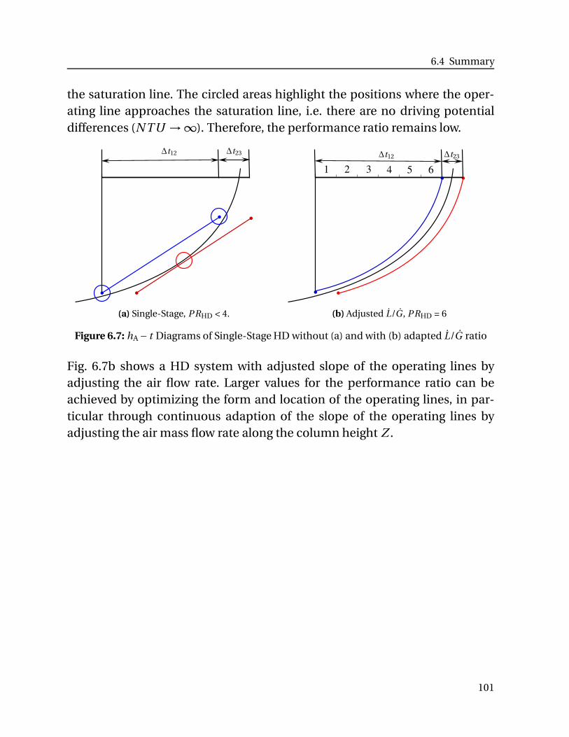
6.4 Summary
the saturation line. The circled areas highlight the positions where the oper-ating line approaches the saturation line, i.e. there are no driving potentialdifferences (NTU →∞). Therefore, the performance ratio remains low.
∆t12 ∆t23
(a) Single-Stage, PRHD < 4.
1 2 3 4 5 6
∆t12 ∆t23
(b) Adjusted L/G , PRHD = 6
Figure 6.7: hA − t Diagrams of Single-Stage HD without (a) and with (b) adapted L/G ratio
Fig. 6.7b shows a HD system with adjusted slope of the operating lines byadjusting the air flow rate. Larger values for the performance ratio can beachieved by optimizing the form and location of the operating lines, in par-ticular through continuous adaption of the slope of the operating lines byadjusting the air mass flow rate along the column height Z .
101

Analysis
102
7 Conclusions
The scope of this thesis is to investigate compact humidification-dehumidi-fication (HD) desalination systems with natural convection through applyingexperimental and analytical methods to contribute towards performance im-provements for HD systems.
Conclusions from literature are limited because of the complex interlinkedheat and mass transfer processes, especially for natural convection. Thiswork combines methods to simulate and visualize the heat and mass transfercorrelations and to interpret the experimental results. These methods are usedto evaluate the influence of the water inlet temperature, the main processparameter for the chosen setups on a single- and two-stage HD configuration.
The analysis of the performance of HD systems is usually based on the con-densate mass flow rate MCond. The determination of this value is associatedwith high measurement inaccuracies and long measurement intervals, espe-cially in the case of small systems, which hinders its applicability. Therefore,an adapted performance ratio P RHD is derived, requiring only a ratio of watertemperature differences. The input values can be constantly measured withhigh accuracy. The differences based on the definitions of both performanceratios are small compared to the measurement inaccuracies for the conven-tional performance ratio. Thus, the adapted performance ratio P RHD is thekey indicator for performance improvements.
To create higher feed water inlet temperatures, brine water is recirculated. Asthe mean water temperature and the mean air temperature rises, heat andmass transfer processes take place in regions with higher vapor concentration.The feed water mass flow rises as the temperature difference between thefeed water inlet and the constant top brine temperature is reduced and theexternal heating power is kept constant. These effects seem to increase thecondensate mass flow rate. However, experiments show that the performanceratio decreases slightly. Further investigations concern the concept of multi-staging for HD with natural convection, which strives to create optimal air
Conclusions
mass flow rates within each stage. The experimental results show that theimprovements in the upper stage are at the expense of the performance ofthe lower stage so that the overall performance is not improved.
An unexpected observation is dropwise condensation on the polypropylenetubes in the dehumidifier even after years of operation of the HD system.Whilst very high condensation rates are reported in literature for dropwisecondensation of pure vapor, the main reason for low condensation rates inthe experiments is explained by the high concentration of carrier gas. A simplemathematical approach is derived to account for this phenomenon.
To analyse and visualize the occurring heat and mass transfer processesthe concept of operating lines is applied. This is combined with analyticalmodeling of the humidification and dehumidification process. Computationof heat and mass transfer along the height of the humidifier and dehumidifiercolumns considers the temperature at the interface between water and air.The interface temperature is essential to numerically determine the heat andmass transfer in water and air.
The performance ratio P R of the investigated HD system with naturalconvection is limited to relatively low values. The cause for the low perfor-mance ratio is mainly due to the small transfer surfaces, transfer coefficientsand the unsatisfactory slope of the operating lines along the height of thesystem. Compact HD setups with natural convection face the principallimitation that the air flow is self regulated according to system configurationsand process conditions.
Future research should focus on HD systems operating in forced convectionand the ability to continuously adjust the air flow rate to optimize the operat-ing lines. The analytical models and methodologies presented in this work canbe applied to HD systems with forced convection to improve the performanceratio.
HD technology is already today used for a range of applications, such as theproduction of drinking water or the concentration of industrial liquids. Itis predestined for the integration with solar water-heaters or solar-thermalpower-plants which provides opportunities for further deployment.
104
Bibliography
Bibliography
[1] H. B. Bacha, M. Boutguedna, M. S. Abid, and A. Y. Maalej. “Modelling and simulationof a water desalination station with solar multiple condensation evaporation cycletechnique”. In: Renewable Energy 18 (1999), pp. 349–365.
[2] H. B. Bacha, M. Bouzguenda, T. Damak, M. S. Abid, and A. Y. Maalej. “Study of awater desalination station using the SMCEC technique: Production optimisation”. In:Renewable Energy 21 (2000), pp. 523–536.
[3] H. D. Baehr. Thermodynamik. 10th ed. Springer-Verlag Berlin, Heidelberg, 2000.
[4] H. D. Baehr and K. Stephan. Wärme- und Stoffübertragung. 4th ed. Springer-VerlagBerlin, Heidelberg, 2004.
[5] W. Beitz and K.-H. Grote. Dubbel - Taschenbuch für den Maschinenbau. 19th ed.Springer-Verlag Berlin, Heidelberg, 1997.
[6] F. Bosnjakovic. Technische Thermodynamik II. Steinkopf Verlag Dresden, Leipzig, 1965.
[7] K. Bourouni, M. Chaibi, and L. Tadrist. “Water desalination by humidification anddehumidification of air: State of the art”. In: Desalination 137 (2001), pp. 167–176.
[8] K. Bourouni, R. Martin, L. Tadrist, and H. Tadrist. “Experimental investigation of evap-oration performances of a desalination prototype using the aero-evapo-condensationprocess”. In: Desalination 114 (1997), pp. 111–128.
[9] T. Brendel. German Patent: DE 10215079B5 - Verfahren zum Destillieren oder Entsalzenvon Flüssigkeiten. 2006.
[10] T. Brendel. “Solare Meerwasserentsalzungsanlagen mit mehrstufiger Verdunstung”.PhD thesis. Ruhr Universität Bochum, 2003.
[11] V. P. Carey. Liquid-Vapor Phase-Change Phenomena: An Introduction to the Thermo-physics of Vaporization and Condensation Processes in Heat Transfer Equipment. Seriesin Chemical, Mechanical Engineering, Taylor, and Francis, 1992.
[12] E. Chafik. “A new seawater desalination process using solar energy”. In: Desalination153 (2002), pp. 25–37.
[13] K. Chehayeb and J. H. Lienhard V. “Effect of Feed Salinity on the Performance ofHumidification Dehumidification Desalination”. In: The IDA World Congress on De-salination and Water Reuse. 2016.
Bibliography
[14] A. Cipollina, G. Micale, and L. Rizzuti, eds. Seawater Desalination - Conventional andRenewable Energy Processes. Springer-Verlag Berlin, Heidelberg, 2009.
[15] H. Czichos and M. Hennecke, eds. HÜTTE – Das Ingenieurwissen. Die Grundlagen derIngenieurwissenschaften. 33rd ed. Springer-Verlag Berlin, Heidelberg, 2008.
[16] Y. J. Dai, R. Z. Wang, and H. F. Zhang. “Parametric analysis to improve the perfor-mance of a solar desalination unit with humidification and dehmudification”. In: De-salination 142 (2002), pp. 107–118.
[17] Y. J. Dai and H. F. Zhang. “Experimental investigation of a solar desalination unit withhumidification and dehumidification”. In: Desalination 130 (2000), pp. 169–175.
[18] B. Dawoud, Y. H. Zurigat, B. Klitzing, T. Aldoss, and G. Theodoridis. “On the possi-ble techniques to cool the condenser of seawater greenhouses”. In: Desalination 195(2006), pp. 119–140.
[19] H. T. El-Dessouky. “Humidification-dehumidification desalination process usingwaste heat from a gas turbine”. In: Engineering Journal of Qatar University (1989),pp. 203–221.
[20] H. T. El-Dessouky and H. M. Ettouney. Fundamentals of Salt Water Desalination. Else-vier, New York, USA, 2002.
[21] H. T. El-Dessouky and H. M. Ettouney. “Plastic/compact heat exchangers for single-effect desalination systems”. In: Desalination 122 (1999), pp. 271–289.
[22] L. L. Diezel. “Untersuchung der Leistungssteigerung des MVC-Prozesses zur Meer-wasserentsalzung über die Erzielung von Tropfenkondensation mittels Ionenimplan-tation”. PhD thesis. Friedrich-Alexander-Universität Erlangen-Nürnberg, 2011.
[23] J. A. Duffie and W. A. Beckman. Solar Engineering of Thermal Processes. John Wiley andSons, Inc., Hoboken, New Jersey, 2006.
[24] H. Emmons. “The mechanism of drop condensation”. In: Transactions, American In-stitute of Chemical Engineers 35 (1939), pp. 109–125.
[25] G. Al-Enezi, H. M. Ettouney, and N. Fawzy. “Low temperature humidification de-humidification desalination process”. In: Energy Conversion and Management 47(2006), pp. 470–484.
[26] S. Ergun. “Fluid flow through packed columns”. In: Chemical Engineering Progress 48(1952), pp. 89–94.
[27] A. Eucken. Lehrbuch der chemischen Physik, Band 2/2 Kondensierte Phasen und Het-erogene Systeme. Akademische Verlagsgesellschaft, 1949.
[28] M. M. Farid and A. W. Al-Hajaj. “Solar desalination with humidification-dehumidifi-cation cycle”. In: Desalination 106 (1996), pp. 427–429.
[29] M. M. Farid, S. Parekh, J. R. Selman, and S. Al-Hallaj. “Solar desalination with a humidi-fication-dehumidification cycle: Mathematical modeling of the unit”. In: Desalination(2003), pp. 153–164.
106
Bibliography
[30] I. Garaway and G Grossmann. “Investigation of a solar-powered desalination systememploying regeneration”. In: Desalination 197 (2006), pp. 63–74.
[31] L García-Rodríguez. “Renewable energy applications in desalination: state of the art”.In: Solar Energy 75 (2003), pp. 381–393.
[32] H. P. Garg, R. S. Adhikari, and R. Kumar. “Experimental design and computer simu-lation of multi-effect humidification (MEH)-dehumidification solar distillation”. In:Desalination 153 (2002), pp. 81–86.
[33] P. Grassmann. Physikalische Grundlagen der Verfahrenstechnik. 2nd ed. Verlag Sauer-länder, Aarau und Frankfurt am Main, 1970.
[34] D. W. Green, ed. Perry’s Chemical Engineers Handbook. 8th ed. McGraw-Hill, New Yorketc., 2007.
[35] U. Grigull. Technische Thermodynamik. Sammlung Goeschen 2170. Walter de Gruyter,Berlin, 1977.
[36] H. Groeber, S. Erk, and U. Grigull. Grundgesetze der Wärmeübertragung. 3rd ed.Springer-Verlag Berlin, Heidelberg, 1962.
[37] K.-H. Grote and J. Feldhusen. Dubbel - Taschenbuch für den Maschinenbau. 23rd ed.Springer-Verlag Berlin, Heidelberg, 2011.
[38] W. N. Grune, R. A. Collins, and T. L. Thompson. “Forced convection, multiple effectsolar still for desalting sea and brackish waters”. In: Proceedings of the United NationsConference on New Sources of Energy E35–S14 (1961), pp. 1–26.
[39] S. Al-Hallaj, M. M. Farid, and A. R. Tamimi. “Solar Desalination with humidificiation–dehumidification cycle: performance of the unit”. In: Desalination 120 (1998), pp. 273–280.
[40] A. H. Hassabou. “Experimental and numerical analysis of a PCM-supported humidi-fication-dehumidification solar desalination system”. PhD thesis. Technische Univer-sität München, 2012.
[41] R. Hauenschild. “Übereinstimmung zwischen Theorie und Praxis bei Merkel-Zahlnachgewiesen”. In: Brennstoff-Wärme-Kraft (1986), pp. 1–5.
[42] M. Hermann, J. Koschikowski, and M. Rommel. “Corrosion-free solar collectors forthermally driven seawater desalination”. In: Solar Energy 75 (2002), pp. 415–426.
[43] O. Heschl and R. Sizman. “Solar Desalination with Recovery of Heat of Condensation”.In: Tagungsbericht 5 - Internationales Sonnenforum, Berlin (1984), p. 375.
[44] C. N. Hodges and W. L. Collins. “Solar Desalination Experience of University of Arizona– Summary: General”. In: Circum-Pacific Energy and Mineral Resources A175 (1976),p. 73.
[45] C. N. Hodges, J. E. Grob, and T. T. Lewis. “Solar Powered Humidification CycleDesalination”. In: Proceedings of the First International Symposium on Water De-salination. 1965, pp. 429–455.
107
Bibliography
[46] C. N. Hodges, T. L. Thompson, J. E. Groh, and D. H. Frieling. “Solar Distillation UtilizingMultiple-Effect Humidification”. In: University of Arizona, Tuscon, Arizona (1966).
[47] C. N. Hodges, T. L. Thompson, J. E. Groh, and W. D. Sellers. “The Utilization of SolarEnergy in a Multiple-Effect Desalinization System”. In: Journal of Applied Science 3(1964), pp. 505–512.
[48] S. Hou. “Two-stage solar multi-effect humidification dehumidification desalinationprocess plotted from pinch analysis”. In: Desalination 222 (2008), pp. 572–578.
[49] S. Hou, S. Ye, and H. Zhang. “Performance optimization of solar humidification–de-humidification desalination process using pinch technology”. In: Desalination 183(2005), pp. 143–149.
[50] S. Hou, D. Zeng, S. Ye, and H. Zhang. “Exergy analysis of the solar multi-effecthumidification-dehumidification desalination process”. In: Desalination (2007),pp. 403–409.
[51] Human Development Report 2015: Work for Human Development. UN DevelopmentProgramme (UNDP), 2015.
[52] S. Kalogirou. “Solar Thermal collectors and application”. In: Energy and CombustionScience 30 (2004), pp. 231–295.
[53] S. Kalogirou. “Use of parabolic trough solar energy collectors for sea-water de-salination”. In: Applied Energy 60 (1998), pp. 65–88.
[54] A. B. Kananeh. “Experimental study of dropwise condensation on ion implanted hor-izontal single tubes and tube bundles”. PhD thesis. Universität Erlangen-Nürnberg,2005.
[55] M. Khedr. “Techno-Economic investigation of an air humidification-dehumidificationdesalination process”. In: Chemical Engineering & Technology 16 (1993), pp. 270–274.
[56] F. Kiefer, F. Schummer, A. Praebst, M. Spinnler, and T. Sattelmayer. “Optimization ofMulti-Effect Vacuum Membrane Distillation Systems for Highly Concentrated Aque-ous Electrolyte Solutions in Liquid Desiccant Air Conditioning and Zero Liquid Dis-charge”. In: Desalination for the Environment Clean Water and Energy. 2016.
[57] J. F. Klausner and R. Li Yi.and Mei. “Evaporative heat and mass transfer for the diffusiondriven desalination process”. In: Heat and Mass Transfer 42 (2006), pp. 528–536.
[58] J. F. Klausner, Y. Li, M. Darwish, and R. Mei. “Innovative diffusion driven desalinationprocess”. In: Journal of Energy Resources Technology 126 (2004), pp. 219–225.
[59] J. C. Kloppers and D. G. Kröger. “The Lewis factor and its influence on the performanceprediction of wet-cooling towers”. In: International Journal of Thermal Sciences 44(2005), pp. 879–884.
[60] A. Kolb. Theoretische und experimentelle Untersuchungen an einem neuen solarenLuftkollektor mit durchströmtem Absorber. Reihe 6: Energietechnik, Nr. 356. VDIVerlag Düsseldorf, 1997.
108
Bibliography
[61] A. Leipertz. Wärme- und Stoffübertragung. ESYTEC, 2008.
[62] Y. Li, J. F. Klausner, R. Mei, and J. Knight. “Direct contact condensation in packed beds”.In: International Journal of Heat and Mass Transfer 49 (2006), pp. 4751–4761.
[63] G. O. G. Löf. Demineralization of saline water with solar energy. Saline Water Conver-sion Program, Research and Development Progress Report No. 4. US Dep. of Interior,1954.
[64] J. Mackowiak. Fluiddynamik von Füllkörpern und Packungen. Springer-Verlag Berlin,Heidelberg, 2009.
[65] J. Mackowiak. “Modellierung des flüsigkeitsseitigen Stoffüberganges in Kolonnen mitklassischen und gitterformigen Füllkörpern”. In: Chemie Ingenieur Technik 80 (2008),pp. 57–77.
[66] M. Mehrgoo and M. Amidpour. “Constructal design and optimization of a direct con-tact humidification–dehumidification desalination unit”. In: Desalination 293 (2012),pp. 69–77.
[67] A. B. Meinel and M. P. Meinel. Applied Solar Energy - An Introduction. Addison-WesleyPublishing Company, Reading etc., 1979.
[68] F. Merkel. Verdunstungskühlung. VDI Forschungsheft Nr. 275. VDI-Verlag, Düsseldorf,1925.
[69] A. Mersmann. Thermische Verfahrenstechnik. Grundlagen und Methoden. Springer-Verlag Berlin, Heidelberg, 1980.
[70] A. M. I. Mohamed and N. A. S. El-Minshawy. “Humidification–dehumidification de-salination system driven by geothermal energy”. In: Desalination 249 (2009), pp. 602–608.
[71] H. Müller-Holst. “Mehrfacheffekt–Entfeuchtluftdestillation bei Umgebungsdruck– Verfahrensoptimierung und Anwendungen”. PhD thesis. Technische UniversitätMünchen, 2002.
[72] H. Müller-Holst. “Solar thermal desalination using the multiple effect humidification(MEH) method”. In: Solar Desalination for the 21st Century: A Review of Modern Tech-nologies and Researches on Desalination Coupled to Renewable Energies. Ed. by L.Rizzuti, Ettourney H.M., and A. Cipollina. Springer-Verlag Berlin, Heidelberg, 2007,pp. 215–225.
[73] A. S. Nafey, H. E. S. Fath, S. O. El-Helaby, and A. Soliman. “Solar desalination usinghumidification-dehumidification processes. Part II. An experimental investigation”.In: Energy Conversion and Management 45 (2004), pp. 1263–1277.
[74] A. Nafey, H. Fath, S. El-Helaby, and A. Soliman. “Solar desalination using humidifi-cation dehumidification processes. Part I. A numerical investigation”. In: Energy Con-version and Management 45 (2004), pp. 1243–1261.
109
Bibliography
[75] G. P. Narayan, R. K. McGovern, J. H. Lienhard V, and S. M. Zubair. “Helium as CarrierGas in Humidification Dehumidification Desalination Systems”. In: Proceedings of theASME 2011 International Mechanical Engineering Congress and Exposition IMECE,Denver, USA (2011).
[76] G. P. Narayan, R. K. McGovern, J. H. Lienhard V, and S. M. Zubair. “Variable pressurehumidification dehumidification desalination system”. In: Proceedings of the ASME /JSME 8th Thermal Engineering Joint Conference AJTEC, Honolulu, Hawaii, USA (2011),pp. 1–11.
[77] G. P. Narayan, R. K. McGovern, G. P. Thiel, J. A. Miller, J. H. Lienhard V, M. H. Sharqawy,S. M. Zubair, and M. A. Antar. “Status of humidification dehumidification desalinationtechnology”. In: IDA World Congress on Desalination 366 (2011).
[78] G. P. Narayan, M. H. Sharqawy, S. Lam, S. K. Das, and J. H. Lienhard V. “Bubble columnsfor condensation at high concentrations of noncondensable gas: Heat-transfer modeland experiments”. In: AIChE Journal 59 (2013), pp. 1780–1790.
[79] G. P. Narayan, M. H. Sharqawy, J. H. Lienhard V, and S. M. Zubair. “Thermodynamicanalysis of humidification dehumidification desalination cycles”. In: Desalination andWater Treatment 16 (2010), pp. 339–353.
[80] G. P. Narayan, M. H. Sharqawy, E. K. Summers, J. H. Lienhard V, S. M. Zubair, and M. A.Antar. “The potential of solar-driven humidification-dehumidification desalinationfor small-scale decentralized water production”. In: Renewable and Sustainable EnergyReviews 14 (2010), pp. 1187–1201.
[81] N. K. Nawayseh, M. M. Farid, S. Al-Hallaj, and A. R. Al-Timimi. “Solar desalinationbased on humidification process – I. Evaluating the heat and mass transfer coeffi-cients”. In: Energy Conversion Management 40 (1999), pp. 1423–1439.
[82] N. K. Nawayseh, M. M. Farid, A. A. Omar, and A. Sabirin. “Solar desalination based onhumidification process. II computer simulation”. In: Energy Conversion Management40 (1999), pp. 1441–1461.
[83] N. K. Nawayseh, M. Farid, A. Omar, and S. Al-Hallaj. “A simulation study to improvethe performance of a solar humidification-dehumidification desalination unit con-structed in Jordan”. In: Desalination 109 (1997), pp. 277–284.
[84] S. Parekh, M. M. Farid, J. R. Selman, and S. Al-Hallaj. “Solar desalination with humidi-fication-dehumidification cycle – a comprehensive technical review”. In: Desalination160 (2004), pp. 167–186.
[85] W. I. Ratzel. “Kunststoffe in der Solartechnik”. In: Proceedings 2nd International SolarForum, Deutsche Gesellschaft für Sonnenenergie, München 1 (1978), pp. 181–193.
[86] M. Rausch. “Grundlegende Untersuchungen zur Ursache von Tropfenkondensationan durch Ionenimplantation modifizierten Metalloberflächen”. PhD thesis. Friedrich-Alexander-Universität Erlangen-Nürnberg, 2010.
110
Bibliography
[87] M. Rommel, M. Köhl, W. Graf, C. Wellens, and F. Brucker. “Corrosion-free collectorswith selectively coated plastic absorbers”. In: Desalination 109 (1997), pp. 149–155.
[88] T. Sattelmayer. Technische Thermodynamik - Energielehre und Stoffverhalten. Lehrstuhlfür Thermodynamik, 2012.
[89] E. Schmidt, W. Schurig, and W. Sellschopp. “Versuche über die Kondensation vonWasserdampf in Film-und Tropfenform”. In: Forschung im Ingenieurwesen (1930),pp. 53–63.
[90] B. Seifert, A. Kroiss, M. Spinnler, and T. Sattelmayer. “About the History of Humi-dification-Dehumidification Desalination Systems”. In: The IDA World Congress onDesalination and Water Reuse. 2013.
[91] B. Seifert, P. Schaufuss, M. Spinnler, and T. Sattelmayer. “CFD Simulation of a Humidi-fication-Dehumidification Desalination Plant for Transient Solar Irradiation”. In: TheIDA World Congress on Desalination and Water Reuse. 2009.
[92] B. Seifert, M. Wenzel, R. Gobitz-Pfeiffer, M. Spinnler, and T. Sattelmayer. “CFD Simu-lation of a HDH-Desalination Plant for Transient Solar Irradiation”. In: The IDA WorldCongress on Desalination and Water Reuse. 2011.
[93] S. M. Soufari, M. Zamen, and M. Amidpour. “Performance optimization of the humi-dification-dehumidification desalination process using mathematical programming”.In: Desalination 237 (2009), pp. 305–317.
[94] M. Spinnler, J. Blumenberg, W. Moik, H. Müller-Holst, and H. U. Krispler. “Small-scalesystems for solar-thermal desalination of sea and brackish water”. In: India NarosaPublishing House, Renewable Energy Technologies Millenium Int. Conference on Re-newable Energies (2000), pp. 179–189.
[95] S. G. Talbert, J.A. Eibling, and G.O.G. Loef. “Manual on solar distillation of saline wa-ter”. In: Office of Saline Water, Reseach and Development Report Report No. 456 (1970).
[96] G. N. Tiwari and A. K. Tiwari. Solar Distillation Practice for Water Desalination Systems.Anshan Pub., 2008.
[97] R. E. Treybal. Mass-Transfer Operations. McGraw-Hill Book Co, 1952.
[98] E. Tzen and R. Morris. “Renewable energy sources for desalination”. In: Solar Energy75 (2003), pp. 375–379.
[99] VDI-Gesellschaft, ed. VDI-Wärmeatlas (German Edition). 10. Edition. Springer-VerlagBerlin, Heidelberg, 2006.
[100] Water Desalination Technologies in the ESCWA Member Countries. United Nations,2001.
[101] I. Watson, O. J. Moarin, and L Henthorne. Desalting Handbook for Planners. 3. UnitedStates Department of the Interior, 2003, p. 310.
[102] D. Wernicke. Methoden und Strategien zur Beurteilung von Abnahmeversuchen anNaßkühltürmen. Forschungsheft Nr. 367. VDI Verlag Düsseldorf, 1997.
111
Bibliography
[103] C. YamalI and I. Solmus. “A solar desalination system using humidification-dehumi-dification process: experimental study and comparison with the theoretical results”.In: Desalination 220 (2008), pp. 538–551.
[104] M. Zamen, M. Amidpour, and S. M. Soufari. “Experimental investigation of a two-stagesolar humidification dehumidification desalination process”. In: Proceedings of ECOS,Italy (2012).
112
List of Figures
List of Figures
1.1 Schematic Setup CA-WH HD-Configuration . . . . . . . . . . . . 2
1.2 tA-X Diagram of Humid Air for Various Relative Humidity Values 4
2.1 Proposed HD Classifications . . . . . . . . . . . . . . . . . . . . . 7
2.2 Closed-Air Water-Heated HD System Overview . . . . . . . . . . 8
2.3 Multi-Stage Configurations of HD Systems . . . . . . . . . . . . . 17
3.1 Temperature-Entropy Diagram of Pure Water . . . . . . . . . . . 21
3.2 Film and Dropwise Condensation on Tubes . . . . . . . . . . . . 25
3.3 Dropwise Condensation in Absence of NCG . . . . . . . . . . . . 26
3.4 Contact Angle and Surface Tensions Droplet . . . . . . . . . . . . 27
3.5 Characteristic Density Profile in HD . . . . . . . . . . . . . . . . . 31
4.1 Evaporation Conditions of Water and Air Flow in Humidifier . . 37
4.2 Control Volumes Humidifier . . . . . . . . . . . . . . . . . . . . . 39
4.3 Control Volumes Humidification . . . . . . . . . . . . . . . . . . . 41
4.4 Computational Chart of 1-D Model for HD . . . . . . . . . . . . . 42
4.5 Example 1-D Simulation Temperature Profile Humidifier . . . . 43
List of Figures
4.6 Schematic Humidifier for Integral Energy Balance . . . . . . . . . 44
4.7 Operating Line for Humidifier . . . . . . . . . . . . . . . . . . . . 45
4.8 Schematic Dehumidifier for Integral Energy and Mass Balance . 46
4.9 Schematic Overview Energy Transfer in HD . . . . . . . . . . . . 48
4.10 Differential Control Volume Dehumidifier at Interface . . . . . . 48
4.11 Heat and Mass Transfer Dehumidification . . . . . . . . . . . . . 49
4.12 Film Condensation With and Withouth NCG . . . . . . . . . . . . 51
4.13 Pressure Profile in Dehumidifier (Humid Air Side) . . . . . . . . . 52
4.14 Heat and Mass Transfer Surfaces Dropwise Condensation . . . . 52
4.15 Modelling of Dropwise Condensation . . . . . . . . . . . . . . . . 53
4.16 Operating Line and Tie Line for Humidifier . . . . . . . . . . . . . 56
4.17 Example Tie Line 1-D Simulation . . . . . . . . . . . . . . . . . . . 57
5.1 Photos Experimental Setups . . . . . . . . . . . . . . . . . . . . . . 62
5.2 Experimental Test Setup . . . . . . . . . . . . . . . . . . . . . . . . 63
5.3 Field Test Single-Stage HD System, Greece . . . . . . . . . . . . . 67
5.4 Humidifier Packing (Hewitech NC20) . . . . . . . . . . . . . . . . 69
5.5 Distribution System . . . . . . . . . . . . . . . . . . . . . . . . . . 70
5.6 Experimental Setup Dehumidifier for Single-Stage . . . . . . . . 71
5.7 Foto of Dropwise Condensation on Plastic Tubes . . . . . . . . . 75
5.8 Experimental Temperature Profiles Single-Stage . . . . . . . . . . 79
5.9 Experimental Temperature Profiles Two-Stage . . . . . . . . . . . 80
5.10 Example Condensate Mass Flow . . . . . . . . . . . . . . . . . . . 81
114
List of Figures
6.1 Overview Mass and Heat Flows in HD . . . . . . . . . . . . . . . . 84
6.2 P RHD Comparison Single Stage and Two Stage HD System . . . . 88
6.3 Overview Operating Lines Single-Stage and Two-Stage . . . . . . 93
6.4 hA− t Diagram Single-Stage CA HD System . . . . . . . . . . . . . 94
6.5 hA− t Diagram Two-Stage CA HD System . . . . . . . . . . . . . . 95
6.6 HTU Plot . . . . . . . . . . . . . . . . . . . . . . . . . . . . . . . . . 99
6.7 hA− t Diagram Overview . . . . . . . . . . . . . . . . . . . . . . . . 101
115

List of Figures
116

Appendix
Appendix
Performance Ratio versus Gained Output Ratio Appendix
A Performance Ratio P R versus Gained
Output Ratio GOR
The performance ratio should not be substituted with the gained output ratioGOR. Large-scale thermal desalination plants, such as multi-stage flash (MSF)or multi-effect distillation (MED), use pressurized high temperature steam(from power plants) as external heat source. The GOR characterizes the multi-effectiveness of a desalination plant as it relates the produced condensatemass flow MDist to the amount of required heating steam mass flow MSteam:
GOR ≡MDist
MSteam. (A.1)
The GOR relates masses or mass flows to express multi-effectiveness wherebythe P R relates energies. Translating the mass flows into energy flows based onthe stored energy in each mass flow ultimately results to an equation similarto the performance ratio. Therefore, the nominal value of GOR is similar to P Rbut should only be used for systems which require heating steam as externalheat source.
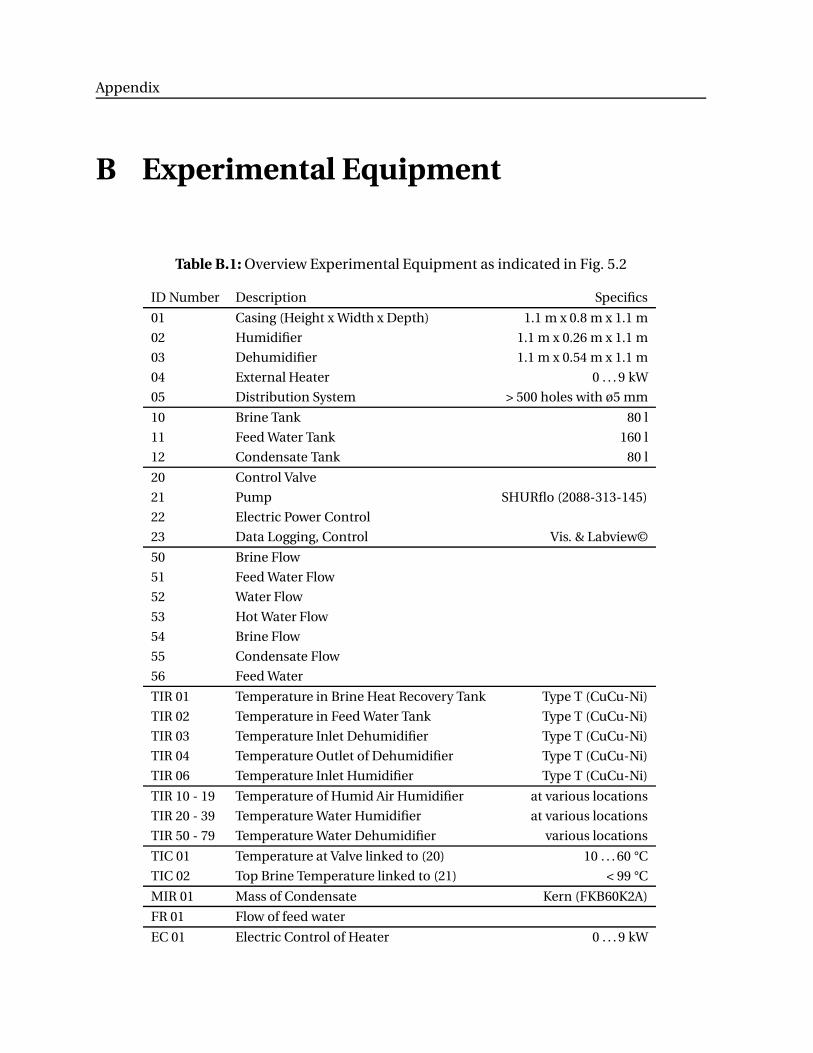
Appendix
B Experimental Equipment
Table B.1: Overview Experimental Equipment as indicated in Fig. 5.2
ID Number Description Specifics
01 Casing (Height x Width x Depth) 1.1 m x 0.8 m x 1.1 m
02 Humidifier 1.1 m x 0.26 m x 1.1 m
03 Dehumidifier 1.1 m x 0.54 m x 1.1 m
04 External Heater 0 . . . 9 kW
05 Distribution System > 500 holes with ø5 mm
10 Brine Tank 80 l
11 Feed Water Tank 160 l
12 Condensate Tank 80 l
20 Control Valve
21 Pump SHURflo (2088-313-145)
22 Electric Power Control
23 Data Logging, Control Vis. & Labview©
50 Brine Flow
51 Feed Water Flow
52 Water Flow
53 Hot Water Flow
54 Brine Flow
55 Condensate Flow
56 Feed Water
TIR 01 Temperature in Brine Heat Recovery Tank Type T (CuCu-Ni)
TIR 02 Temperature in Feed Water Tank Type T (CuCu-Ni)
TIR 03 Temperature Inlet Dehumidifier Type T (CuCu-Ni)
TIR 04 Temperature Outlet of Dehumidifier Type T (CuCu-Ni)
TIR 06 Temperature Inlet Humidifier Type T (CuCu-Ni)
TIR 10 - 19 Temperature of Humid Air Humidifier at various locations
TIR 20 - 39 Temperature Water Humidifier at various locations
TIR 50 - 79 Temperature Water Dehumidifier various locations
TIC 01 Temperature at Valve linked to (20) 10 . . . 60 °C
TIC 02 Top Brine Temperature linked to (21) < 99 °C
MIR 01 Mass of Condensate Kern (FKB60K2A)
FR 01 Flow of feed water
EC 01 Electric Control of Heater 0 . . . 9 kW
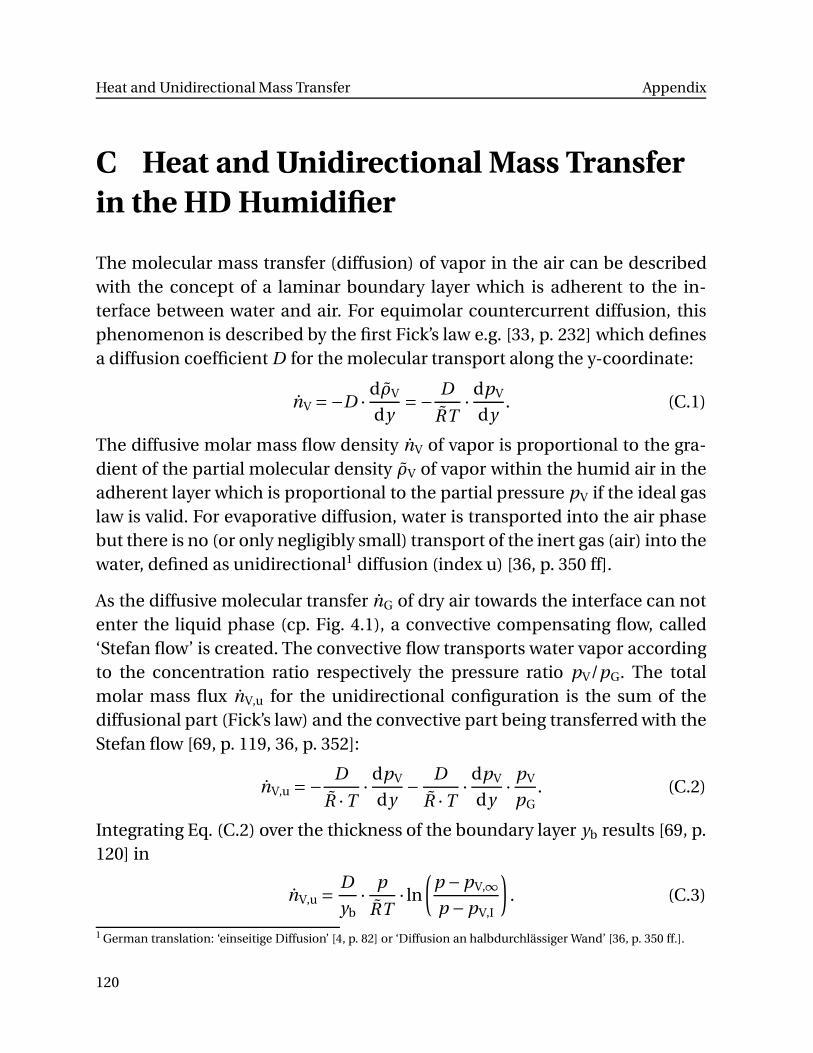
Heat and Unidirectional Mass Transfer Appendix
C Heat and Unidirectional Mass Transfer
in the HD Humidifier
The molecular mass transfer (diffusion) of vapor in the air can be describedwith the concept of a laminar boundary layer which is adherent to the in-terface between water and air. For equimolar countercurrent diffusion, thisphenomenon is described by the first Fick’s law e.g. [33, p. 232] which definesa diffusion coefficient D for the molecular transport along the y-coordinate:
nV =−D ·dρV
dy=−
D
RT·
dpV
dy. (C.1)
The diffusive molar mass flow density nV of vapor is proportional to the gra-dient of the partial molecular density ρV of vapor within the humid air in theadherent layer which is proportional to the partial pressure pV if the ideal gaslaw is valid. For evaporative diffusion, water is transported into the air phasebut there is no (or only negligibly small) transport of the inert gas (air) into thewater, defined as unidirectional1 diffusion (index u) [36, p. 350 ff].
As the diffusive molecular transfer nG of dry air towards the interface can notenter the liquid phase (cp. Fig. 4.1), a convective compensating flow, called‘Stefan flow’ is created. The convective flow transports water vapor accordingto the concentration ratio respectively the pressure ratio pV/pG. The totalmolar mass flux nV,u for the unidirectional configuration is the sum of thediffusional part (Fick’s law) and the convective part being transferred with theStefan flow [69, p. 119, 36, p. 352]:
nV,u =−D
R ·T·
dpV
dy−
D
R ·T·
dpV
dy·
pV
pG. (C.2)
Integrating Eq. (C.2) over the thickness of the boundary layer yb results [69, p.120] in
nV,u =D
yb·
p
RT· ln
(p −pV,∞
p −pV,I
)
. (C.3)
1 German translation: ‘einseitige Diffusion’ [4, p. 82] or ‘Diffusion an halbdurchlässiger Wand’ [36, p. 350 ff.].
120

Appendix
This can be approximated from a series expansion for the logarithmic expres-sion:
nV,u ≈ nV ·1
1−pV,m/p. (C.4)
Hereby, the partial pressure pV,m is the arithmetic mean value of pv,I and pv,∞.For equimolar mass transfer problems, the mass transfer coefficient β is ap-plied which is related to the concentration differences between interface andbulk air flow respectively to the partial density differences ρV,I −ρV,∞ [69, p.116] with vapor as ideal gas:
mV =β ·(
ρV,I −ρV,∞
)
=β ·pV,I −pV,∞
RV ·T. (C.5)
The mass transfer coefficient β corresponds to the heat transfer coefficientα in heat transfer correlations, as described in chapter C. For unidirectionaltransfer, the ‘Stefan flow’ increases the molar transfer of the vapor approxi-mately with the factor 1/(1−pV,m/p). According to Eq. (C.4) the mass transfercoefficient for evaporation is:
mV,u =βu ·pV,I −pV,∞
RV ·T≈β ·
pV,I −pV,∞
RV ·T · (1−pV,m/p). (C.6)
The analogy between heat and mass transfer is given due to the similar differ-ential equations for heat and equimolar mass transfer, if the boundary con-ditions are identical. The heat transfer equation for a dependency only iny-direction can be written [36, p. 344] as
q =α · (T1 −T2)=−a ·d(ρ ·h)
dy, (C.7)
with the heat transfer coefficient α and the thermal diffusivity a = λ/(ρ · cp).The corresponding mass transfer equation according to first Fick’s law forequimolar countercurrent flow is
m =β · (ρ1 −ρ2) =−D ·dρ
dy. (C.8)
121
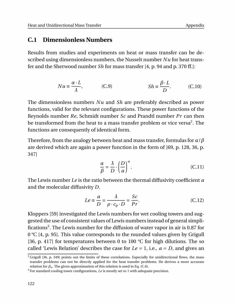
Heat and Unidirectional Mass Transfer Appendix
C.1 Dimensionless Numbers
Results from studies and experiments on heat or mass transfer can be de-scribed using dimensionless numbers, the Nusselt number Nu for heat trans-fer and the Sherwood number Sh for mass transfer [4, p. 94 and p. 370 ff.]:
Nu ≡α ·L
λ, (C.9) Sh ≡
β ·L
D. (C.10)
The dimensionless numbers Nu and Sh are preferably described as powerfunctions, valid for the relevant configurations. These power functions of theReynolds number Re, Schmidt number Sc and Prandtl number Pr can thenbe transformed from the heat to a mass transfer problem or vice versa2. Thefunctions are consequently of identical form.
Therefore, from the analogy between heat and mass transfer, formulas for α/βare derived which are again a power function in the form of [69, p. 128, 36, p.347]
α
β=
λ
D·
(D
a
)n
. (C.11)
The Lewis number Le is the ratio between the thermal diffusivity coefficient aand the molecular diffusivity D .
Le ≡a
D=
λ
ρ · cp ·D=
Sc
Pr. (C.12)
Kloppers [59] investigated the Lewis numbers for wet cooling towers and sug-gested the use of consistent values of Lewis numbers instead of general simpli-fications3. The Lewis number for the diffusion of water vapor in air is 0.87 for0 °C [4, p. 95]. This value corresponds to the rounded values given by Grigull[36, p. 417] for temperatures between 0 to 100 °C for high dilutions. The socalled ‘Lewis Relation’ describes the case for Le = 1, i.e., a = D , and gives an2 Grigull [36, p. 349] points out the limits of these correlations. Especially for unidirectional flows, the mass
transfer problems can not be directly applied for the heat transfer problems. He derives a more accuraterelation for βu. The given approximation of this relation is used in Eq. (C.6).
3 For standard cooling tower configurations, Le is mostly set to 1 with adequate precision.
122
Appendix C.2 Lewis Factor for Unidirectional Transport
indication of the ratio between heat and mass transfer [69, p. 128]:
β=α
ρ · cp. (C.13)
This transformation leads to the mass transfer coefficient β for the for theequimolar mass transfer. For unidirectional mass transfer, as it is the casefor humidification and dehumidification, the correction factor needs to beincluded according to Eq. (C.6).
C.2 Lewis Factor Lef,u for Unidirectional Transport
The numerical calculations can be simplified by combining the relations forheat and mass transfer. The Lewis Factor Lef is applicable for this calculationas it relates the heat and mass transfer can be derived from Eq. (C.11) [69, p.128]:
Lef =α
β ·ρ · cp= Le1−n . (C.14)
For evaporation processes, Lewis Factor Lef is calculated according to thecorrelations for the unidirectional flow using the correlation for βu accordingto Eq. (C.6):
Lef,u =α
βu ·ρ · cp= Le1−n ·
(
1−pV,m
p
)−1
. (C.15)
A common definition of the Lewis Factor Lef,u for unidirectional mass transferuses the evaporation coefficient σevap instead of βu. Hauenschild [41] gives therelation between σevap and βu. The mass transfer rate mV is proportional to βu
and also to the partial density difference of water vapor in humid air ∆ρV andto σevap and ∆X ,
σevap =βu ·p
RG ·Tm·
(
1−pV,m
p
)
. (C.16)
with the mean temperature of humid air Tm, the arithmetic mean of the waterand air temperature. The conversion of βu to σevap is shown in Annex C.3. Theunidirectional Lewis Factor Lef,u can be expressed as:
Lef,u =α
σevap · cp·
(
1−pV,m
p
)
. (C.17)
123
Heat and Unidirectional Mass Transfer Appendix
The Lewis Factor Lef,u is used for the derivation of the temperature tI of theinterface I, as shown in Eq. (4.15).
C.3 Correlations for β,βu and σevap
As discussed in chapter C.2, the unidirectional Lewis Factor Lef,u can be ex-pressed with the unidirectional mass transfer coefficientβu or the evaporationcoefficient σevap. Eq. (C.16) expresses σevap as a function of βu and can bederived as follows:
mV =βu ·
(1
RW ·Tm
)
·(
pV,I −pV,∞
)
. (C.18)
mV =σevap · (XI −X∞) =σevap ·MW
MG·
(pV,I
p −pV,I−
pV,∞
p −pV,∞
)
. (C.19)
σevap =
[
βu ·1
RW ·Tm·
RW
RG
]
·(pV,I −pV,∞) ·
(
p −pV,I
)
·(
p −pV,∞
)
pV,I ·(
p −pV,∞
)
−pV,∞ ·(
p −pV,I
) . (C.20)
σevap =βu ·p
RG ·Tm·
(
1−pV,I
p
)
·
(
1−pV,∞
p
)
. (C.21)
with Tm = 0.5 · (TI −T∞) andRG
RW=
MW
MG= 0.622. (C.22)
The unidirectional mass transfer coefficient βu can be expressed with themass transfer coefficient β for equimolar mass flow and a correction factor.This coefficient β can be determined from analogies between heat, mass andmomentum transfer [36, p. 350 ff.]4:
β=βu
p·
pV,I −pV,∞
lnp−pV,∞
p−pV,I
=βu
p·
pG,∞−pG,I
lnpG,∞
pG,I
. (C.23)
The logarithmic mean partial pressure of the carrier gas G between interfaceI and the bulk (index ∞) flow can be approximated for small pressure differ-ences to pV,I [36, p. 354 ff.] leading to a simplified relation for the (unidirec-
4 Grigull [36] labels βh as the mass transfer coefficient for unidirectional diffusion at the semipermeable wall.
124
Appendix C.3 Correlations for β,βu and σevap
tional) evaporation coefficient σevap:
β≈βu ·pG,I
p=βu ·
(
1−pV,I
p
)
. (C.24)
σevap ≈β ·p
RG ·Tm·
(
1−pV,∞
p
)
. (C.25)
The controlling mass transfer coefficient βh and the Lewis Factor Lef werepreviously introduced.
Due to the difference between the temperature of the bulk water flow L and itsinterface (index I) in the humidifier, heat is transferred from the water to theinterface, which can be described principally as convective heat transfer [6]:
Qconv,W =αW · (TW,∞−TI) · Aα. (C.26)
In the gaseous phase, heat is transferred from the interface to the bulk air flow:
Qconv,A =αA · (TI −TA,∞) · Aα. (C.27)
125
![Some improvements of Xfem for cracked domainsmath.univ-lyon1.fr/~renard/papers/2007_CMAS.pdf · Some improvements of Xfem for cracked domains 3. θ ∈ ]−π,π[r crack tip ΓC](https://img.pdfslide.tips/doc/110x75/5aa80e8f7f8b9aca258b5764/some-improvements-of-xfem-for-cracked-renardpapers2007cmaspdfsome-improvements.jpg)