Ph.D. THESISstrana.snu.ac.kr/laboratory/theses/jhkim2018.pdf · 2018-03-05 · measured wind data for reinforced concrete columns. The equivalent static wind pressure is adopted to

Ph.D. THESIS

Wind Load Factor Based on Wind Load Statistics

for Reliability-Based Bridge Design Codes

신뢰도기반 교량설계기준에서

풍하중 통계특성을 고려한 풍하중계수

2018년 2월

서울대학교 대학원

건설환경공학부

김 지 현

ii

ABSTRACT

Wind Load Factor Based on Wind Load Statistics for Reliability-Based Bridge Design Codes

Ji Hyeon Kim

Department of Civil and Environmental Engineering

The Graduate School

Seoul National University

This work presents a general approach for evaluating wind load factors based on

measured wind data for reinforced concrete columns. The equivalent static wind

pressure is adopted to approximate the aerodynamic wind pressure using the gust

factor. The probabilistic model of wind velocity is established based on measured

wind data, and that of wind pressure is constructed by Monte-Carlo simulations.

For calibration of reliability-based wind load factors, the relationship between sta-

tistical parameters of wind velocity and pressure are required. In this study, the

normalized wind pressure is defined to develop the relationships between statistical

parameters of wind velocity and pressure.

The P-M interaction diagrams of the pylons define the limit state function of

the pylons subjected to unaixial bending. The load contour method is utilized to

estimate the strength of a reinforced concrete column subjected to biaxial bending.

Load and strength parameters are considered as random variables in the reliability

analysis. The strength parameters of an RC column include the material proper-

ties and geometric properties of the cross section of an RC column. The Hasofer-

Lind Rackwitz-Fiessler algorithm with the gradient projection method is employed

iii

to calculate the most probable failure point and the reliability index. The continu-

ous and differentiable P-M interaction diagram is constructed with discretely de-

fined sampling points of the P-M interaction diagram using the cubic spline inter-

polation. The sensitivities of the P-M interaction diagram are calculated through

the direct differentiation of the cubic spline and sampling points of the P-M interac-

tion diagram. Detailed expressions of the sensitivities of the P-M interaction dia-

gram with respect to the random variables are presented. Reliability analyses are

carried out by the proposed method to investigate the wind load-governed limit

state for the reinforced concrete pylons of five cable-supported bridges in Korea.

Based on the results of the reliability analysis, dead load factors are set to the

bias factors of dead load components, and a P-M interaction diagram drawn by the

mean values of the strength parameters is used to define a design equation. The

most probable failure point of the wind load is obtained by equating the probability

of non-exceedance of wind load at the most probable failure point to the probabil-

ity of safety corresponding to a given reliability index. An analytical form of the

wind load factor is derived in terms of the statistical parameters of wind load and

the target reliability index. Validity of the proposed load factors is verified

through a reliability assessment of the pylon sections of the five bridges. It is

shown that the proposed load factors secure the target reliability levels within a 2%

error.

The proposed wind load factor is adjusted to be used with the dead load factors

and the resistance factor specified in several reliability-based design codes. The

validity of the adjustment procedure is confirmed by calibrating the wind load fac-

tor for the AASHTO LRFD Bridge Design Specifications. The wind load factor

adjusted for Korean Highway Bridge Design Code (Limit State Design) – Cable-

iv

supported Bridges is presented in terms of the coefficient of variations of the wind

velocity. To adapt the wind load factor as 1.0, the recurrence periods of the basic

wind velocity are calculated to secure target reliability indexes. The analytical

form of determining the basic wind velocity for Korean Highway Bridge Design

Code (Limit State Design), which yields a uniform target reliability level, is pro-

posed by using the statistical parameters of wind load and the adjusted wind load

factors. The validity of the proposed wind load factor is also confirmed through

the reliability assessment of the RC pylons with various sizes of cross-sections.

The reliability indexes of the pylons subjected to biaxial bending are calculated to

investigate the effects of biaxial loads on the reliability level for the wind load

combinations. It is confirmed that the wind load combination allowing vehicular

live loads does not govern the design of pylon sections.

Keywords: Wind load factor; Calibration; Probability of failure; Target reliability

index; Reinforced concrete column; Wind pressure; Reliability analysis; Wind

Load Statistics; Biaxial Load; Reliability-based bridge design codes;

v

TABLE OF CONTENTS

SECTION page

1. INTRODUCTION ................................................................................................. 1

2. WIND LOAD STATISTICS ............................................................................... 14

2.1 Equivalent Static Wind Pressure ................................................................... 16

2.2 Probabilistic Description of Wind Velocity ................................................... 23

2.3 Probabilistic Description of Wind Pressure................................................... 36

3. RELIABILITY ASSESSMENT OF RC COLUMNS ......................................... 44

3.1 Reliability Assessment of RC Columns Subjected to Uniaxial Bending Based

on the P-M Interaction Diagram using AFOSM ........................................... 45

3.1.1 Formulation of the AFOSM for PMID................................................... 46

3.1.2 Approximation of PMID with the Cubic Spline .................................... 52

3.1.3 Sensitivity Calculation ........................................................................... 56

3.2 Reliability Assessment of RC Columns Subjected to Biaxial Bending using

the Load Contour Method ............................................................................. 67

3.2.1 Failure Surface for Biaxial Bending ....................................................... 68

3.2.2 AFOSM and Sensitivity ......................................................................... 73

3.3 Reliability Assessment of RC Pylons for Cable-supported Bridges ............. 76

4. CALIBRATION OF WIND LOAD FACTOR .................................................... 95

4.1 Base Load Factors and Design Equations ..................................................... 96

4.2 Adjustment for AASHTO Specifications .................................................... 105

4.3 Adjustment for KHBDC (LSD) and KHBDC (LSD)-CB ........................... 111

4.3.1 Adjusted wind load factors for KHBDC (LSD)-CB ............................ 111

4.3.2 Adjusted wind load factors and suggested wind velocity for KHBDC (LSD) ..................................................................................................... 123

4.4 Verification for Variations of Cross-sections ............................................... 130

vi

4.4.1 Determination of Sections for Target Reliability ................................. 131

4.4.2 Verifications of Wind Load Factors ..................................................... 134

5. EFFECT OF BIAXIAL BENDING .................................................................. 142

5.1 Reliability Assessment of RC Pylons under Biaxial Bending for UltLS-3 . 143

5.2 Reliability Assessment of RC Pylons under Biaxial Bending for UltLS-5 . 158

6. CONCLUSIONS AND RECOMMENDATIONS FOR FURTHER STUDY .. 164

REFERENCES ...................................................................................................... 170

APPENDIX ........................................................................................................... 176

A. Stress-strain Relations of KHBDC ............................................................... 176

vii

LIST OF FIGURES

Figure page

Fig. 2.1 Empirical cumulative frequency and the theoretical CDF of the annual

maximum V10 for IB .................................................................................... 30


maximum V10 for BHB ............................................................................... 31


maximum V10 for UB .................................................................................. 31


maximum V10 for YSB ................................................................................ 32


maximum V10 for NMB .............................................................................. 32

Fig. 2.6 Annual maximum V10 for IB plotted on probability paper ......................... 33

Fig. 2.7 Annual maximum V10 for BHB plotted on probability paper .................... 33

Fig. 2.8 Annual maximum V10 for UB plotted on probability paper ....................... 34

Fig. 2.9 Annual maximum V10 for YSB plotted on probability paper ..................... 34

Fig. 2.10 Annual maximum V10 for NMB plotted on probability paper .................. 35

Fig. 2.11 Bias factor of the wind pressure and mean of the normalized wind

pressure ....................................................................................................... 41

Fig. 2.12 COV of the wind pressure ........................................................................ 42

Fig. 2.13 Normalized wind pressure for NMB on the probability paper ................ 42

Fig. 3.1 Typical cross-section of an RC column: (a) definition of geometric

properties; and (b) variation of strain in a section. ...................................... 46

Fig. 3.2. Modified Newton-Raphson method with double iteration loops. ............. 49

viii

Fig. 3.3 Construction of the PMID using the cubic spline interpolation ................. 54

Fig. 3.4 Stress-strain diagram: (a) reinforcing steel for tension and compression;

and (b) parabola-rectangle diagram for concrete under compression. ........ 60

Fig. 3.5 Failure surface of RC columns subjected to biaxial bending and

compression ................................................................................................. 68

Fig. 3.6 Normalized load contours for different values of α ................................... 70

Fig. 3.7 General view of cable-supported bridges and longitudinal wind direction:

(a) IB; (b) BHB; (c) UB; (d) YSB; (e) NMB (Unit: m) .............................. 83

Fig. 3.8 Front view of the pylon and transverse wind load direction: (a) IB; (b)

BHB; (c) UB; (d) YSB; (e) NMB (Unit: m) ................................................ 84

Fig. 3.9 Geometry and rebar arrangement of the bottom section for the pylon: (a)

IB; (b) BHB; (c) UB; (d) YSB; (e) NMB (Unit: mm) ................................. 85

Fig 3.10 Comparison of convergence rates ............................................................. 88

Fig. 3.11 PMIDs and failure point of the design section of IB................................ 90

Fig. 3.12 PMIDs and failure point of the design section of BHB ........................... 90

Fig. 3.13 PMIDs and failure point of the design section of UB .............................. 91

Fig. 3.14 PMIDs and failure point of the design section of YSB ............................ 91

Fig. 3.15 PMIDs and failure point of the design section of NMB .......................... 92

Fig 3.16 Variations of reliability indexes and normalized MPFPs for IB ............... 92

Fig 3.17 Variations of reliability indexes and normalized MPFPs for BHB ........... 93

Fig 3.18 Variations of reliability indexes and normalized MPFPs for UB .............. 93

Fig 3.19 Variations of reliability indexes and normalized MPFPs for YSB ............ 94

Fig 3.20 Variations of reliability indexes and normalized MPFPs for NMB .......... 94

Fig. 4.1 Variation of Kgb with the target reliability index ........................................ 99

Fig. 4.2 Variation of base wind load factors and calculated reliability indexes for

ix

given wind load factors (λWS = 1) ............................................................. 102

Fig. 4.3 Determination of the wind load factor for the AASHTO specifications

(YSB) ........................................................................................................ 109

Fig. 4.4 Adjusted wind load factors and best-fit lines for the AASHTO

specifications (λWS = 1.0) .......................................................................... 109

Fig. 4.5 Variation of the adjusted wind load factor for the AASHTO specifications

(λWS = 0.875, δWS = 0.2) ............................................................................ 110

Fig 4.6 Adjusted wind load factors and best-fit lines for KHBDC (LSD)-CB (λWS =

1.0, αWS = 0.80) ......................................................................................... 119

Fig. 4.7 Difference of factored load effects for KHBDC (LSD) and KHBDC

(LSD)-CB for YSB (λWS = 1.0, δWS = 0.30, λWS = 1.0, βT = 3.1) ............. 119

Fig. 4.8 Variation of wind load factors for KHBDC (LSD)-CB ........................... 120

Fig. 4.9 Best-fit-line of the coefficient of Kgb(βT) in Eq. (4.14) ........................... 120

Fig. 4.10 Best-fit-line of Kgb(βT) in Eq. (4.14) ..................................................... 121

Fig. 4.11 Difference between the adjusted and approximated wind load factors for

KHBDC (LSD)-CB ................................................................................... 121

Fig. 4.12 Variation of the inverse CDF of Gumbel distribution for various

recurrence periods of the basic wind velocity ........................................... 122

Fig. 4.13 Variation of the reliability index for various recurrence periods of the

basic wind velocity .................................................................................... 122

Fig. 4.14 Adjusted wind load factors and best-fit lines for KHBDC (LSD) (λWS =

1.0, αWS = 0.82) ......................................................................................... 129

Fig. 4.15 Comparison of the design PMIDs drawn by two provisions for YSB ... 129

Fig. 4.16 Variations of dimensional scales for the optimum sections: (a) IB; (b) UB

x

................................................................................................................... 138

Fig. 4.17 Optimum section for 4% reinforcement ratio of IB ............................... 139

Fig. 4.18 PMIDs and failure point of the optimum section for IB ........................ 139

Fig. 4.19 Optimum section for 2% reinforcement ratio of UB ............................. 140

Fig. 4.20 PMIDs and failure point of the optimum section for UB....................... 140

Fig. 4.21 Design PMIDs and factored load effects: (a) IB; (b) UB ....................... 141

Fig. 5.1 Reliability indexes of pylons for IB under biaxial bending ..................... 148

Fig. 5.2 Standard normal wind load at the MPFP of pylons for IB under biaxial

bending ...................................................................................................... 148

Fig. 5.3 Nominal bending moments for IB ........................................................... 149

Fig. 5.4 Reliability indexes of pylons for BHB under biaxial bending ................. 150

Fig. 5.5 Standard normal wind load at the MPFP for BHB under biaxial bending

................................................................................................................... 150

Fig. 5.6 Nominal bending moments for BHB ....................................................... 151

Fig. 5.7 Reliability indexes of pylons for UB under biaxial bending.................... 152

Fig. 5.8 Standard normal wind load at the MPFP for UB under biaxial bending . 152

Fig. 5.9 Nominal bending moments for UB .......................................................... 153

Fig. 5.10 Reliability indexes of pylons for YSB under biaxial bending ............... 154

Fig. 5.11 Standard normal wind load at the MPFP for YSB under biaxial bending

................................................................................................................... 154

Fig. 5.12 Nominal bending moments for YSB ...................................................... 155

Fig. 5.13 Reliability indexes of pylons for NMB under biaxial bending .............. 156

Fig. 5.14 Standard normal wind load at the MPFP for NMB under biaxial bending

................................................................................................................... 156

Fig. 5.15 Nominal bending moments for NMB .................................................... 157

xi

Fig. 5.16 Two-dimensional representations of the failure surface for UB: (a) failure

contour; and (b) failure plane PMIDs........................................................ 162

Fig. 5.17 Two-dimensional representations of the failure surface for YSB: (a)

failure contour; and (b) failure plane PMIDs ............................................ 163

Fig. A.1 Stress-strain relation of concrete in KHBDC (LSD) (KMOLIT, 2016a) 176

Fig. A.2 Comparison of the PMIDs for the stress-strain relations ........................ 178

Fig. A.3 PMIDs and failure point of YSB for different design codes ................... 179

xii

LIST OF TABLES

Table page

Table 2.1 Wind velocity profile parameters in KHBDC (LSD)-CB ....................... 20

Table 2.2 Pressure coefficients for five bridges ...................................................... 21

Table 2.3 Gust factors for the IB, UB, YSB, and NMB .......................................... 21

Table 2.4 Exposure coefficients for the UB, YSB, and NMB ................................. 22

Table 2.5 Product of variables except for the pressure coefficient for BHB ........... 22

Table 2.6 Statistical parameters of the calculated and fitted annual maximum V10 at

the bridge sites ............................................................................................. 29

Table 2.7 Results of the goodness-of-fit test and values of likelihood function for

NMB ............................................................................................................ 29

Table 2.8 Statistical parameters of the fitted Gumbel for maximum V10 ................ 30

Table 2.9 Statistical parameters of the coefficients in Eq. (2.1) .............................. 40

Table 3.1 Inclined angle of the pylons and sectional properties of the design

sections ........................................................................................................ 86

Table 3.2 Statistical parameters of the random variables ........................................ 86

Table 3.3 Design VB and statistical characteristics of the wind load ....................... 87

Table 3.4 Load effect matrices under the design VB in the longitudinal direction .. 87

Table 3.5 Load effect matrices under the design VB in the transverse direction ..... 88

Table 3.6 Reliability indexes of the design sections................................................ 89

Table 3.7 Normalized MPFP of the design sections ................................................ 89

Table 4.1 Reliability index and the MPFP of wind load ......................................... 97

Table 4.2 Unit normal vector of the limit state functions at the MPFP ................... 98

Table 4.3 Base and adjusted wind load factors for three βT and δWS .................... 102

xiii

Table 4.4 Load effect matrices for λWS = 1.0 in transverse direction .................... 103

Table 4.5 Load effect matrices for λWS = 1.0 in longitudinal direction ................. 103

Table 4.6 Results of the validation analysis for the base load factor ( 49.2~ =γWS

,δWS = 0.3) .................................................................................................. 104

Table 4.7 Results of adjustment for the AASHTO specifications (βT = 3.1, δWS =

0.3) ............................................................................................................ 108

Table 4.8 Dead load factors in various design specifications ................................ 117

Table 4.9 Results of adjustment for KHBDC (LSD)-CB (βT = 3.1, δWS = 0.3) .... 118

Table 4.10 Adjusted wind load factors for three βT and αWS for KHBDC (LSD)–CB

and KHBDC (LSD) ................................................................................... 118

Table 4.11 KR and βT for various recurrence periods of the basic wind velocity for

wind load factor of 1.0 in the rage of 13.010.010

≤δ≤ V .......................... 118

Table 4.12 Results of the adjustment for KHBDC (LSD) (βT = 3.1, δWS = 0.3) ... 127

Table 4.13 Reliability index and statistical parameters of the wind pressure for

KHBDC (LSD) .......................................................................................... 127

Table 4.14 Statistical parameters of the coefficients in Eq. (2.1) for short-to

medium-span bridges ................................................................................ 128

Table 4.15 Suggested basic wind velocity for KHBDC (LSD) (γWS = 1.4) ........... 128

Table 4.16 Basic wind velocity and pressure, its statistical characteristics ........... 136

Table 4.17 Composition of wind load effects ........................................................ 136

Table 4.18 Results of reliability analyses for the adjusted sections in IB and UB 137

Table 4.19 Adjusted and required wind load factors ............................................. 137

Table 5.1 Minimum reliability index of pylons of five bridges (α = 1) ................ 147

xiv

Table 5.2 Comparison of reliability indexes under uniaxial and biaxial bending for

IB ............................................................................................................... 149


BHB ........................................................................................................... 151


UB ............................................................................................................. 153


YSB ........................................................................................................... 155


NMB .......................................................................................................... 157

Table 5.7 Load effect matrix for live load on the central span .............................. 160

Table 5.8 Load effect matrix for live load on the side spans ................................. 161

Table 5.9 Statistical parameters of the random variables ...................................... 161

Table 5.10 Results of the reliability assessment for UltLS-5 ................................ 161

1

SECTION 1

INTRODUCTION

Reliability-based design codes specify many requirements to attain a proper safety

level through design equations. The design equations define relationships be-

tween the nominal strength of a structural member and nominal load effects by us-

ing load-resistance factors. The design equations are usually given in simple line-

ar forms, but the load-resistance factors, which are determined to ensure a certain

reliability level, are derived based on the results of complicated reliability analyses.

Current reliability-based design specifications concern short- to medium-span

bridges, of which the designs are governed by gravitational or earthquake loads

rather than by wind load. Therefore, a precise calibration for the wind load factor

may not be necessary. Although the wind load factor proposed for short- to me-

dium-span bridges is usually applied without justification to the design of wind

load-governed structures such as the pylons of cable-supported bridges, wind load

factors that yield specified target reliability indexes for a wind load-governed limit

state (WGLS) should be defined separately for such structures.

In this work, a determination procedure of wind load factors is proposed for

the WGLS. The probabilistic models of wind velocity and pressure are estab-

lished, and relationships between statistical parameters of wind velocity and pres-

sure are identified. Robust reliability assessment methods are proposed for a rein-

forced concrete (RC) column subjected to uniaxial and biaxial loads, respectively.

The proposed reliability analysis method is applied to assess the reliability indexes

of RC pylons for cable-supported bridges under uniaxial load. Base load factors

and a design equation are proposed based on the results of the reliability analyses.

2

The adjustment procedure is proposed to calibrate wind load factors for current

reliability-based bridge design codes. Biaxial effects on the reliability indexes

are investigated through reliability assessments of the RC pylons subjected to biax-

ial bending. Previous studies for each scope in this thesis are reviewed, and the

methods proposed in this thesis are briefly described next.

Wind load statistics

Statistical relationships between wind velocity and load as well as statistical

models of wind velocity and load are required to evaluate a wind load factor since

the nominal value of wind load is defined by wind velocity in most reliability-

based design specifications (AASHTO, 2012; ACI, 2001; ACI, 2011; BSI, 2001;

CEN, 2004; CSA, 2000; KMOLIT, 2016a). Although statistical models of wind

velocity and/or load have been reported through various studies (Ellingwood et al.,

1980; Ellingwood and Tekie, 1999; Miciarelli et al., 2001; Ellingwood, 2003; Scott

et al., 2003; Bartlett et al., 2003; Diniz et al., 2005; Gabbai et al., 2008; Kwon et al.,

2015), no study on statistical relationships between wind velocity and load have

been founded in the previous studies. In this study, the statistical models of wind

velocity and pressure are developed based on the measured wind data, and the sta-

tistical relationships between them are identified through Monte-Carlo simulations.

The probabilistic model of wind velocity is constructed based on measured

wind data. The Kolmogorov-Smirnov goodness-of-fit test (Ang and Tang, 2007)

is applied to confirm a distribution type of wind velocity. The Gumbel distribu-

tion is selected to describe the distribution type of wind velocity by comparing the

values of likelihood functions (Haldar and Mahadevan, 2000). The statistical pa-

rameters of wind velocity are estimated through a linear regression of cumulative

3

probabilities on the Gumbel probability paper, and the cumulative probabilities of

wind velocity are plotted by the Gringorten plotting positions (Gringorten, 1963).

A nominal value of wind velocity is referred to as a basic wind velocity in the most

design specifications and is generally defined by a recurrence period of wind veloc-

ity and design life of a structure. Since the probability model of wind load is re-

quired to determine a proper probability-based load factor, the statistical relation-

ships between wind velocity and pressure should be identify to calibrate wind load

factors.

The normalized wind pressure, which is obtained by multiplying wind coeffi-

cients and velocity normalized to their mean values, is defined to identify relation-

ships between the statistical parameters of wind velocity and pressure. Since the

uncertainties in the wind coefficients such as analysis coefficient, pressure coeffi-

cient, exposure coefficient, and gust factor contribute to the uncertainty of wind

pressure, Monte-Carlo simulations are adopted to establish a probabilistic model of

the normalized wind pressure based on the statistical distribution of wind coeffi-

cients and velocity. The distribution type of the normalized wind pressure is con-

firmed as the Gumbel distribution through the Kolmogorov-Smirnov goodness-of-

fit test with significance level of 0.01. The linear regression of the cumulative

probabilities by the Gringorten plotting positions is used to estimate the statistical

parameters of the normalized wind pressure. The relationships between the statis-

tical parameters of wind velocity and pressure are investigated based on the results

of Monte-Carlo simulations. The mean value of the normalized wind pressure is

presented as a linear function of the COV of wind velocity by the best-fit line.

The bias factor of wind pressure is expressed by a function of the bias factor for the

basic wind velocity and the mean value of the normalized wind pressure, while the

4

COV of wind pressure is equal to that of the normalized wind pressure. In case

that the design life of a structural is identical to the return period of the basic wind

velocity, the bias factor of wind pressure corresponding to the basic wind velocity

is simply formed as a linear function of the COV of the wind velocity. The COV

of wind pressure is presented as linear functions of the COV of wind velocity, of

which range is determined based on the measured wind data. The relationships

between the statistical parameter of wind velocity and pressure are valid regardless

of the design life of a structure and can be used in calibration of wind load factor.

Reliability assessment of RC columns for uniaxial bending

From columns of buildings to pylons of cable-supported bridges, various types

of RC columns are designed based on the P-M interaction diagrams (PMID)

(Nilson et al., 2010), which define the limit states of columns subject to combined

axial and bending actions. Since the failure of a column may result in the total

collapse of a structure, the precise estimation of the failure point of a column is one

of the most important issues in the design and the reliability assessment of a col-

umn, especially in code calibrations.

Various approaches (Frangopol et al., 1996; Hong and Zhou, 1999; Jiang and

Yang, 2013; Milner et al., 2001; Mirza, 1996; Stewart and Attard, 1999; Szerszen et

al., 2005) have been proposed to evaluate reliability indexes of RC columns sub-

jected to uniaxial bending since the statistical characteristics of the strengths of RC

columns were evaluated through Monte-Carlo simulations by Ellingwood (1977)

and Grant et al. (1978). Stewart and Attard (1999) and Szerszen et al. (2005) as-

sumed the eccentricity of total load effect, which is the ratio of bending moment to

axial force, to be a deterministic variable for the reliability assessment of RC col-

5

umns. The uncertainty of the eccentricity was taken into account in the works by

Hong and Zhou (1999) and Jiang and Yang (2013). Mirza (1996) estimated the

moment capacities of RC columns for a fixed axial force, while Frangopol et al.

(1996) and Milner et al. (2001) performed the reliability analyses for load paths

determined by load correlations. The statistical characteristics of the strength of

an RC column are obtained through Monte-Carlo simulations (Ellingwood, 1977;

Frangopol et al., 1996; Grant et al., 1978; Milner et al., 2001; Mirza, 1996; Stewart

and Attard, 1999; Szerszen et al., 2005).

The aforementioned studies are based on one common assumption that the

strength of an RC column can be pre-determined on the PMID by a load condition.

That is, the strength of an RC column can be defined as an intersection point in the

P-M space between the PMID and a straight line connecting the origin and total

load effect (Hong and Zhou, 1999; Jiang and Yang, 2013; Stewart and Attard, 1999;

Szerszen et al., 2005) or between the PMID and pre-defined load path (Frangopol

et al., 1996; Milner et al., 2001; Mirza, 1996). With this assumption, the limit

state function of an RC column is simply expressed as the assumed strength minus

the total load effect applied to the column, which is an approximation of a real limit

state function but a convenient form to apply a traditional reliability analysis

scheme. However, the approximated limit state function may lead to erroneous

results because the real strength of an RC column at failure depends on not only the

total load effect but also the statistical characteristics of all random variables. The

PMID itself defines the failure and safe states of an RC column, and thus the PMID

of an RC column should be adopted as the limit state function for accurate reliable

assessment. Another shortcoming of the previous studies is that statistical varia-

tions are applied directly to internal forces (Frangopol et al., 1996; Hong and Zhou,

6

1999; Jiang and Yang, 2013; Milner et al., 2001; Mirza, 1996; Stewart and Attard,

1999; Szerszen et al., 2005). Since the internal forces simply represent the load

effects induced by the external load components, the load components should be

chosen as independent random variables rather than internal forces, and thus the

statistical variations should be taken into account in the individual load component.

The author and coworkers (Kim et al., 2015) proposed a new approach in order

to estimate the most probable failure point (MPFP) and reliability index of a short

RC column, in which the nonlinear P-delta effect can be neglected, based on the

advanced first-order second-moment reliability method (AFOSM) (Haldar and

Mahadevan, 2000). The PMID of an RC column is adopted as the limit state

function for the AFOSM without employing any assumption on the strength of an

RC column, and external load components rather than internal forces are selected

as independent random variables. The PMID representing the column strength

depends upon the material and geometric properties of cross section of a column,

which are also considered as random variables. The material properties include

the compressive strength of concrete, the Young’s modulus and the yield strength

of each reinforcing bar. Meanwhile, the gross area of a cross section, the areas

and the locations of reinforcing bars are the random variables on the geometric

properties. The proposed method does not require Monte-Carlo simulations to

obtain the statistical properties of the column strength. The reliability indexes are

directly calculated in the AFOSM using the sensitivities of the PMID with respect

to random variables. Since the PMID is generally nonlinear with respect to the

random variables, the Hasofer-Lind-Rackwitz-Fiessler (HL-RF) algorithm with the

gradient projection method (Liu and Der Kiureghian, 1991) is adopted to solve the

minimization problem that defines the MPFP in the AFOSM.

7

The HL-RF algorithm requires the first-order sensitivities of the PMID with re-

spect to the random variables. However, the PMID is defined at discrete sampling

points corresponding to given locations of the neutral axis of a cross section.

Therefore, a continuous and differentiable PMID should be constructed with the

discrete sampling points to calculate the sensitivities of the PMID. The cubic

spline interpolation (Kreyszig, 2006), which is the collection of piecewise cubic

polynomials interpolating two adjacent sampling points of the PMID, is employed.

The coefficients of the cubic spline are determined based on the continuity re-

quirements up to the second-order derivatives at the boundaries between two adja-

cent segments of the cubic spline. The direct differentiation of each segment of

the cubic spline with respect to the random variables yields the sensitivities of the

PMID required in the AFOSM.

Evaluation of wind load factors

All load and resistance factors in reliability-based design specifications should

be determined so as to satisfy a target reliability index specified for the correspond-

ing limit state. For instance, the target reliability index for the limit state gov-

erned by gravitational loads such as dead and vehicular live loads is clearly defined

in most recent reliability-based design specifications (AASHTO, 2014; ASCE,

2013; CEN, 2002), and a great deal of research has been performed on the target

reliability index as well as on the load and resistance factors for the limit state.

Unfortunately, the target reliability index for the WGLS is rarely defined in most

current design specifications, and a robust procedure to evaluate the load and re-

sistance factors for the WGLS has not been reported.

A limited number of studies have dealt with wind load factors. Minciarelli et

8

al. (2001) defined the wind load factor as the ratio of the wind load effect induced

by wind velocity with a 500-year to 50-year mean recurrence interval, which was

also adopted by Diniz and Simiu (2005) and Gabbai et al. (2008). However, the

reliability level secured by the proposed wind load factor was not discussed in their

studies. Nowak (1999) and Bartlett et al. (2003) proposed a wind load factor for

the WGLS, but they did not present the details of their calibration process. In the

studies of Ellingwood et al. (1980) and Ellingwood and Tekie (1999), the MPFP of

a wind load was assumed without clear justification in their evaluation of the wind

load factor.

The author and coworkers (Kim et at., 2017) proposed a general approach for

evaluating the load factors of the WGLS in the along-wind direction for given reli-

ability indexes using measured wind data, based on the results of the reliability as-

sessment for RC pylons of cable-supported bridges in Korea. The RC pylons of

five cable-supported bridges in Korea are selected as typical wind-load governed

structural components for the calibration of the wind load factor. Wind acting on

structures induces the dynamic wind pressure in addition to the static wind pressure

due to the aerodynamic effect of wind. Since, however, wide-ranging parameters

on structural systems and bridge sites influence the dynamic wind pressure, the

generalized statistical model of the dynamic wind pressure is not available at the

present time. Consequently, the dynamic wind pressure cannot be explicitly in-

cluded in the calibration of the wind load factor for all-purpose reliability-based

bridge design specifications. To circumvent this limitation, most of the previous

works (Bartlett et al., 2003; Diniz and Simiu, 2005; Ellingwood et al., 1980;

Ellingwood and Tekie, 1999; Gabbai et al., 2008; Minciarelli et al., 2001) on the

wind load factor in the along-wind direction are based on an equivalent static wind

9

pressure, which is obtained by multiplying the gust factor to the static wind pres-

sure on structural members (Simiu and Scanlan, 1996) and this study also adopts a

similar approach. The gust factor plays the same role as the dynamic impact fac-

tor (dynamic load allowance) used to model the dynamic effect of vehicular live

loads.

It is shown that the failure of a pylon is caused by a dominant increase of the

wind load while the other random variables remain near their mean values.

Therefore, the MPFPs of all random variables other than the wind load are assumed

to be their mean values. With this assumption, the dead load factors become the

bias factors of the corresponding dead load components, and the PMID constructed

with the mean values of the strength parameters of a pylon section is used to de-

scribe a design equation. Here, the design equation indicates the criterion that a

total factored load should satisfy. By utilizing the geometric interpretation of the

reliability index, the MPFP of the wind load is obtained by equating the non-

exceedance probability at the MPFP of wind load to the probability of safety of a

pylon section corresponding to the target reliability index. The wind load factor is

derived by dividing the MPFP of wind load by the nominal value of wind load, and

is expressed in an analytical form in terms of the target reliability index and the

statistical parameters of the wind load.

The proposed wind load factor is adjusted for the AASHTO LRFD Bridge De-

sign Specifications (AASHTO specifications, AASHTO, 2014), in which the dead

load factors of both the wind load- and gravitational load-governed limit states are

identical, and the design equation is defined with the design PMID. The validity

of the proposed load factors and adjusted wind load factor for the AASHTO speci-

fications is demonstrated. The pylon sections designed with the proposed wind

10

load factors for three different reliability indexes are examined whether they secure

the specified target reliability indexes. The proposed wind load factors and the

adjusted load factors result in pylon sections that satisfy the specified target relia-

bility indexes within an acceptable error range of less than 2%.

The proposed adjustment procedure is applied to evaluate the adjusted wind

load factors for Korean Highway Bridge Design Code (Limit State Design)-Cable-

supported Bridge (KHBDC (LSD)-CB) (KMOLIT, 2016b) and Korean Highway

Bridge Design Code (Limit State Design) (KHBDC (LSD)) (KMOLIT, 2016a).

The wind load factor corresponding to the basic wind velocity and target reliability

index specified in KHDBC (LSD)-CB is derived as a linear function of the COV of

wind velocity based on the statistical relationships between wind velocity and pres-

sure. The reliability indexes secured by the basic wind velocity and the wind load

factor given in KHBDC (LSD) are identified. Since the reliability index obtained

by the basic wind velocity in KHBDC (LSD) varies significantly depending on

regions, an analytical form of the basic wind velocity is derived so as to yield a

uniform reliability level for a given wind load factor.

The validity of the adjusted wind load factor is confirmed for various sizes of a

cross-section. The adjusted wind load factor is compared with the required wind

load factor which satisfies the design equation for the strength of the cross-section

determined to satisfy a target reliability index. The cross-sections securing a tar-

get reliability index for given reinforcement ratios are determined by adjusting the

geometric properties of the section based on the method proposed by Choi (2016).

It is verified that the adjusted wind load factor yields the required wind load factor

within 3% error.

11

Reliability assessment of RC columns for biaxial bending

Various external loads applied to columns generally induce biaxial bending.

Recent reliability-based design specifications and standards (AASHTO, 2012; ACI,

2001; ACI, 2011; BSI, 2001; CEN, 2004; CSA, 2000; KMOLIT, 2016a) provide

design criteria for the design of RC columns subjected to axial force and biaxial

bending. The load contour method and the reciprocal load method proposed by

Bresler (1960) are widely employed to define the strengths of RC columns subject-

ed to biaxial bending. The reciprocal load method describes the relation between

the ultimate axial strength of an RC column and the eccentricity of axial force.

The load contour defines the failure surface of an RC column subjected to biaxial

bending with a family of curves using a surface exponent and P-M interaction dia-

grams for uniaxial bending (PMIDU) with respect to two principal axes of a cross-

section.

The reciprocal load method has a limitation in terms of general applicability

because it is unable to estimate the strength of an RC column subjected to biaxial

bending induced by lateral load independent of axial force. Moreover, it is gener-

ally known that the reciprocal load method may yield erroneous results for columns

subjected to strong bending (Hassoun and Al-Manaseer, 2012; McCormac and

Brown, 2014; Nilson et al., 2010; Wang and Salmon, 1992), and that the load con-

tour method is applicable to a wider range of load effects than the reciprocal load

method. This is why some design specifications (BSI, 2001; CEN, 2004; CSA,

2000; KMOLIT, 2016a) adopt only the load contour method while other specifica-

tions (AASHTO, 2012; ACI, 2001; ACI, 2011) define the strength of an RC col-

umn by both methods depending on the magnitude of axial force.

Some succeeding studies on the load contour method have been reported

12

(Bonet et al., 2014; Hsu, 1986; Hsu, 1988; Pannell, 1963; Parme and Nieves, 1966).

Pannell (1963) and Parme and Nieves (1966) proposed approximated values of the

surface exponent for the load contour method by graphical representations. Hsu

(1986 and 1988) formulated a simplified version of the load contour method with a

fixed surface exponent. Bonet et al. (2014) presented analytical expressions of

the surface exponent in terms of a reinforcement ratio. Although such studies

have been reported, the load contour method proposed by Bresler (1960) is com-

monly adopted in recent reliability-based design codes (AASHTO, 2012; ACI,

2001; ACI, 2011; BSI, 2001; CEN, 2004; CSA, 2000; KMOLIT, 2016a) to define

the strength of RC columns under biaxial bending.

Various approaches for assessing the reliability of RC columns subjected to

uniaxial bending are available (Frangopol et al., 1996; Hong and Zhou, 1999; Jiang

and Yang, 2013; Milner et al., 2001; Mirza, 1996; Stewart and Attard, 1999;

Szerszen et al., 2005). However, the reliability levels of RC columns subjected to

biaxial bending has been rarely reported except for one conference paper (Wang

and Hong, 2002) that showed a simplified approach based on the reciprocal load

method. The reliability levels of RC columns need to be evaluated accurately to

determine a proper resistance factor and a target reliability index for various limit

states used in reliability-based code calibration.

The author and coworker (Kim and Lee, 2017) suggested a robust reliability

assessment approach of RC columns subjected to biaxial bending based on the

AFOSM. The failure surface defined in the load contour method acts as the limit

state function for the reliability analysis. The load parameters, the eccentricities

of axial forces, the geometric and material properties of RC columns are selected as

random variables. The Hasofer-Lind-Rackwitz-Fiessler (HL-RF) algorithm with

13

the gradient projection method is utilized to solve the minimization problem for the

AFOSM. Since the failure surface of an RC column subjected to biaxial bending

is constructed with the PMID for uniaxial bending with respect to each principal

axis of a cross-section, reliability analyses of biaxially loaded RC columns heavily

rely on those for uniaxial bending. The cubic spline interpolation is adopted to

form the PMID subjected to uniaxial load, and the sensitivities of the failure sur-

face to the random variables are obtained by the direct differentiation method.

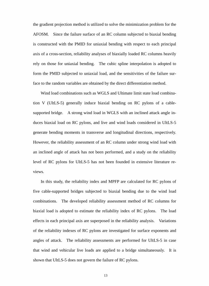
Wind load combinations such as WGLS and Ultimate limit state load combina-

tion V (UltLS-5) generally induce biaxial bending on RC pylons of a cable-

supported bridge. A strong wind load in WGLS with an inclined attack angle in-

duces biaxial load on RC pylons, and live and wind loads considered in UltLS-5

generate bending moments in transverse and longitudinal directions, respectively.

However, the reliability assessment of an RC column under strong wind load with

an inclined angle of attack has not been performed, and a study on the reliability

level of RC pylons for UltLS-5 has not been founded in extensive literature re-

views.

In this study, the reliability index and MPFP are calculated for RC pylons of

five cable-supported bridges subjected to biaxial bending due to the wind load

combinations. The developed reliability assessment method of RC columns for

biaxial load is adopted to estimate the reliability index of RC pylons. The load

effects in each principal axis are superposed in the reliability analysis. Variations

of the reliability indexes of RC pylons are investigated for surface exponents and

angles of attack. The reliability assessments are performed for UltLS-5 in case

that wind and vehicular live loads are applied to a bridge simultaneously. It is

shown that UltLS-5 does not govern the failure of RC pylons.

14

SECTION 2

WIND LOAD STATISTICS

Wind acting on structures induces aerodynamic wind pressure, which consists of

the static as well as dynamic component. The aerodynamic wind pressure de-

pends on structural and site characteristics of a bridge, which cannot be explicitly

included in the calibration of the wind load factor for all-purpose reliability-based

bridge design specifications because numerous problem-dependent statistical vari-

ables on structural systems and bridge sites are involved. Rather, the gust factor

is utilized to represent the aerodynamic wind pressure as the equivalent static wind

pressure in an approximate sense. The gust factor plays a similar role to the dy-

namic impact factor (dynamic load allowance) used to consider the dynamic effect

of vehicular live loads on a structure. The dynamic load effect of the vehicular

live load also depends on the characteristics of the live load itself as well as the

dynamic behaviors of a structure, but the dynamic load effect is modeled by the

dynamic impact factor in the calibration of the vehicular live load factor. This is

because the calibration process becomes too complicated or even impossible to

determine a live load factor, which is exactly the same situation as in the calibra-

tion of the wind load factor.

The statistical model of wind load effect is necessarily developed to calculate

wind load factors for a reliability-based design code, and the statistical model of

wind velocity is required to establish that of wind load effect. Since, however, the

nominal value of wind load is generally specified by wind velocity rather than

wind pressure in many reliability-based design specifications (AASHTO, 2014;

ASCE, 2010; CSA International, 2000; Eurocode 1, 2005; JRA, 2007; KMOLIT,

15

2016a and 2016b; KSCE, 2006 ), a relation between statistical parameters of wind

velocity and pressure should be identified. Although individual statistical models

of the wind velocity and pressure have been reported by many researchers

(Ellingwood et al., 1980; Ellingwood and Tekie, 1999; Miciarelli et al., 2001;

Ellingwood, 2003; Scott et al., 2003; Bartlett et al., 2003; Diniz et al., 2005; Gabaai

et al., 2008; Kwon et al., 2015), no study on the statistical relationships between

wind velocity and pressure has been found in extensive literature reviews. In this

work, the statistical models of the wind velocity and pressure are developed based

on the measured wind data, and the statistical relationships between them are iden-

tified through Monte-Carlo simulations.

Section 2.1 introduces an equivalent static wind pressure for the along-wind di-

rection which is obtained by multiplying the gust factor by the static wind pressure

on structural members. In Section 2.2, the distribution type of wind velocity is

confirmed through goodness-of-fit tests and likelihood functions. The statistical

parameters of wind velocity are estimated by the linear regression on the Gumbel

probability paper. In Section 2.3, the normalized wind pressure is defined by

wind coefficients and velocity normalized to their mean values. The probabilistic

model of the normalized wind pressure is constructed through Monte-Carlo simula-

tions. The goodness-of-fit test and linear regression are utilized to identify the

probabilistic description of the normalized wind pressure. A relation between the

statistical parameters of wind velocity and pressure is investigated based on the

results of Monte-Carlo simulations.

16

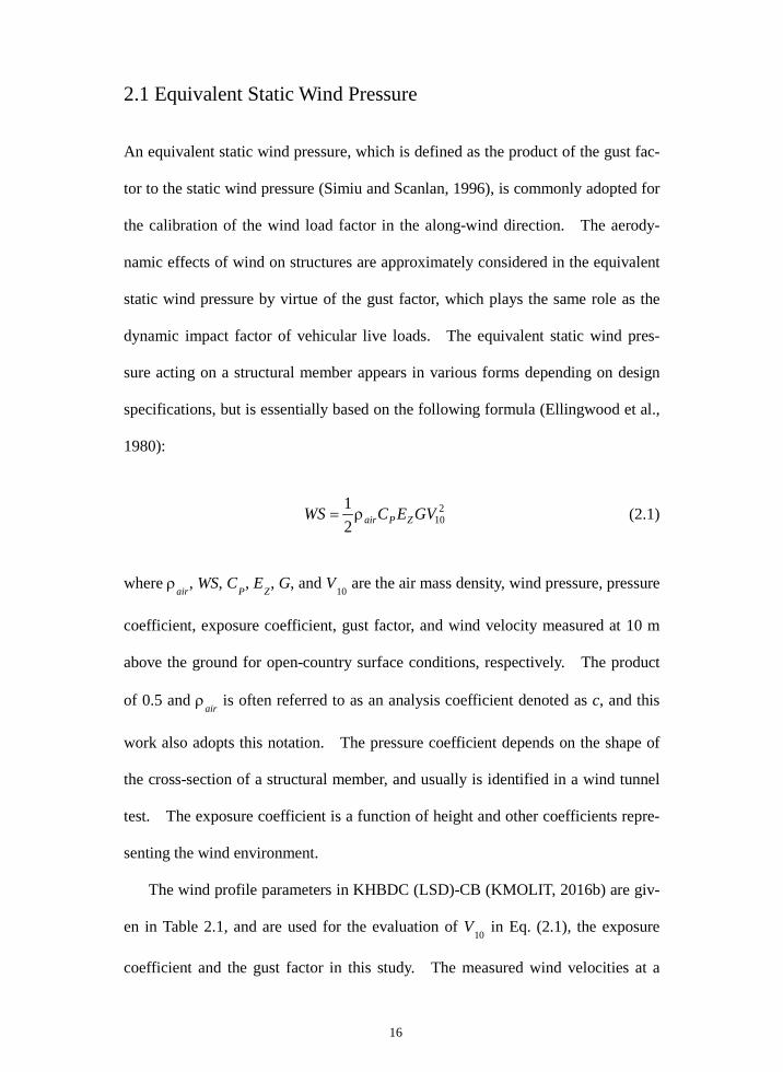
2.1 Equivalent Static Wind Pressure

An equivalent static wind pressure, which is defined as the product of the gust fac-

tor to the static wind pressure (Simiu and Scanlan, 1996), is commonly adopted for

the calibration of the wind load factor in the along-wind direction. The aerody-

namic effects of wind on structures are approximately considered in the equivalent

static wind pressure by virtue of the gust factor, which plays the same role as the

dynamic impact factor of vehicular live loads. The equivalent static wind pres-

sure acting on a structural member appears in various forms depending on design

specifications, but is essentially based on the following formula (Ellingwood et al.,

1980):

2

1021 GVECWS ZPairρ= (2.1)

where ρair, WS, CP, EZ, G, and V10 are the air mass density, wind pressure, pressure

coefficient, exposure coefficient, gust factor, and wind velocity measured at 10 m

above the ground for open-country surface conditions, respectively. The product

of 0.5 and ρair is often referred to as an analysis coefficient denoted as c, and this

work also adopts this notation. The pressure coefficient depends on the shape of

the cross-section of a structural member, and usually is identified in a wind tunnel

test. The exposure coefficient is a function of height and other coefficients repre-

senting the wind environment.

The wind profile parameters in KHBDC (LSD)-CB (KMOLIT, 2016b) are giv-

en in Table 2.1, and are used for the evaluation of V10 in Eq. (2.1), the exposure

coefficient and the gust factor in this study. The measured wind velocities at a

17

weather station are transformed to V10 for open-country surface conditions by the

following equation defined in the code.

mm

mG

GV

zz

zV mαα= )()10( ,

II,10

II (2.2)

where α and zG are the parameters in Table 2.1 whereas subscript m and II are used

to indicate those variables for the category corresponding to the location of the

weather station and Category II in the table. Here, zG denotes the gradient wind

level. Also, zm, which is given in meter, represents the measurement height of

wind velocity, and Vm is the measured wind velocity in m/sec. The exposure

coefficient and the gust factor in Eq. (2.1) are expressed in terms of the wind veloc-

ity profile parameters in Table 2.1 as follows:

<

≥

=α

α

bG

b

bG

Z

zzzz

zzzz

Efor )(706.3

for )(706.3

2

2

(2.3)

where z = height at which wind pressure is evaluated; z0 and zb = minimum

height of the boundary layer and the ground surface roughness length, respectively.

The wind profile parameters of the category corresponding to a bridge site should

be selected. The wind profile parameters for Category I are adopted because the

five bridges are constructed in offshore areas.

The gust factor is defined as a function of the turbulence intensity and the

height of a structure in various design codes in order to take into account the dy-

namic effect of the structure for wind load. In Eurocode 1 (CEN, 2010), the gust

18

factor is considered in evaluating the equivalent static wind pressure, and the wind

load effects due to the equivalent static wind pressure are calculated by using both

the gust factor and a structural factor. The structural factor accounts for the effect

of vibrations of a structural due to turbulence as well as the effect of the non-

simultaneous occurrence of peak wind pressure. Eurocode 1 suggests a structural

factor as 1 for low rise buildings and structures with natural frequencies greater

than 5 Hz which are expected to have minimal dynamic effects. The structural

factor for chimneys, high rise buildings, and bridges of constant depth with cross-

sections is suggested as function of the turbulence intensity, the correlation of the

wind pressure on the structure surface, and the turbulence in resonance with the

vibration mode. In ASCE 7 (ASCE, 2013) and Korean Highway Bridge Design

Codes (Limit State Design) (KHBDC (LSD)) (KMOLIT, 2016a), the gust-effect

factor is defined to calculate wind load effects directly due to the equivalent static

wind pressure. ASCE 7 and KHBDC (LSD) recommend that the gust-effect fac-

tor for rigid buildings is adopted as 0.85 or calculated by using a given formula.

For flexible or dynamically sensitive buildings, a resonance response factor, which

is defined to take into account a natural frequency, the damping ratio, and a cross-

sectional shape of a structure, is involved in evaluating the gust-effect factor.

The aforementioned design specifications (CEN, 2010; ASCE, 2013; KMOLIT,

2016a) are developed to directly evaluate the wind load effects rather than the

equivalent static wind pressure for a design of buildings and short- to medium-span

bridges. However, it is impossible to present a general formulation for evaluating

the wind load effects directly for cable-supported bridges, since each cable-

supported bridge is uniquely designed for the type, length, and shape. In the de-

sign of cable-supported bridges, KHBDC (LSD)-CB (KMOLIT, 2016b) provides a

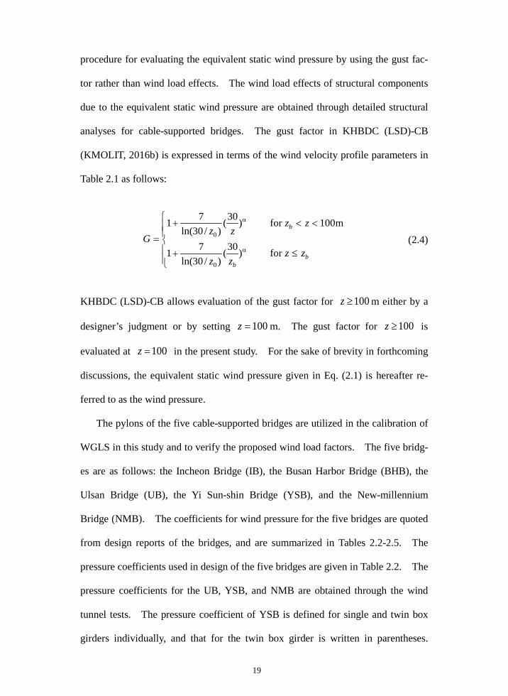
19

procedure for evaluating the equivalent static wind pressure by using the gust fac-

tor rather than wind load effects. The wind load effects of structural components

due to the equivalent static wind pressure are obtained through detailed structural

analyses for cable-supported bridges. The gust factor in KHBDC (LSD)-CB

(KMOLIT, 2016b) is expressed in terms of the wind velocity profile parameters in

Table 2.1 as follows:

≤+

<<+

=α

α

bb

b

zzzz

zzzz

Gfor )30(

)/30ln(71

m100for )30()/30ln(

71

0

0 (2.4)

KHBDC (LSD)-CB allows evaluation of the gust factor for 100≥z m either by a

designer’s judgment or by setting 100=z m. The gust factor for 100≥z is

evaluated at 100=z in the present study. For the sake of brevity in forthcoming

discussions, the equivalent static wind pressure given in Eq. (2.1) is hereafter re-

ferred to as the wind pressure.

The pylons of the five cable-supported bridges are utilized in the calibration of

WGLS in this study and to verify the proposed wind load factors. The five bridg-

es are as follows: the Incheon Bridge (IB), the Busan Harbor Bridge (BHB), the

Ulsan Bridge (UB), the Yi Sun-shin Bridge (YSB), and the New-millennium

Bridge (NMB). The coefficients for wind pressure for the five bridges are quoted

from design reports of the bridges, and are summarized in Tables 2.2-2.5. The

pressure coefficients used in design of the five bridges are given in Table 2.2. The

pressure coefficients for the UB, YSB, and NMB are obtained through the wind

tunnel tests. The pressure coefficient of YSB is defined for single and twin box

girders individually, and that for the twin box girder is written in parentheses.

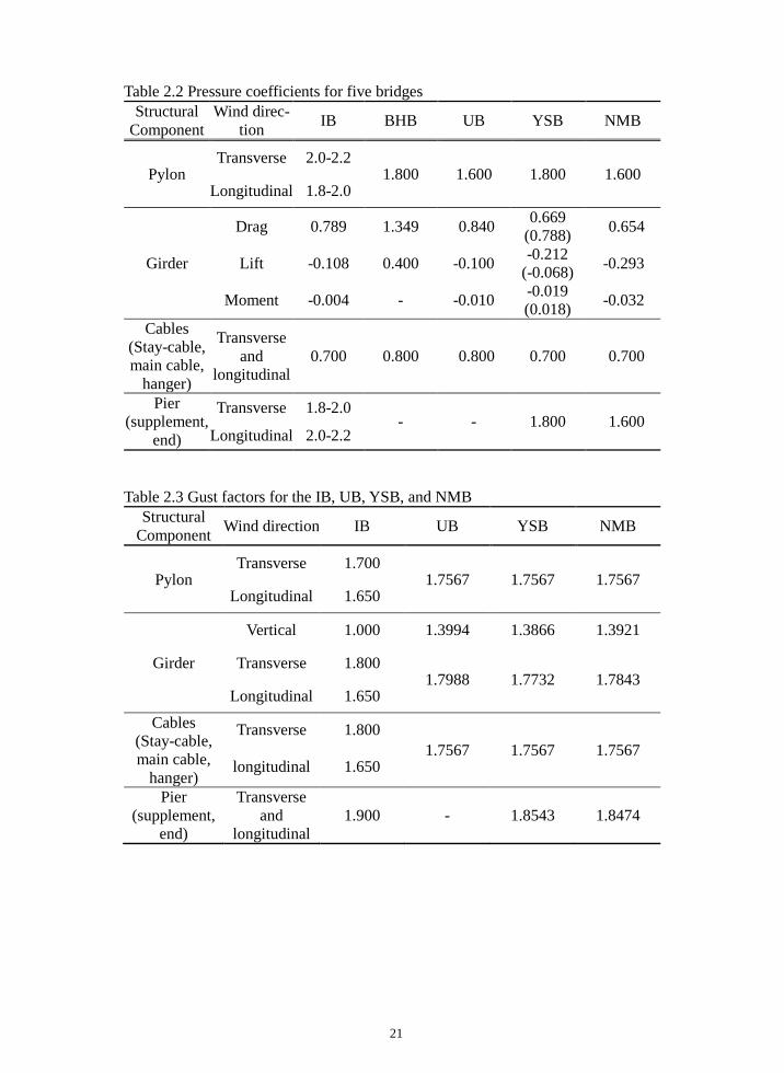
20

The gust factor used in the design of IB, UB, YSB, and NMB are given in Table

2.3. The gust factors of the UB, YSB, and NMB are calculated based on Eq. (2.4),

while those of the IB are obtained through gust response analyses. Table 2.4

shows the exposure coefficients used in the design of the UB, YSB, and NMB

which are evaluated at the representative height of the structural components.

The exposure coefficient for the girder of the IB is calculated as 1.549 at the repre-

sentative height, and those for cables, pylons, and piers of IB are not presented in

the design report. The products of the coefficients for wind pressure except for

the pressure coefficient, which are presented in the design report of the BHB, are

given in Table 2.5.

Table 2.1 Wind velocity profile parameters in KHBDC (LSD)-CB

Category Description α zG (m) zb (m) z0 (m)

I Offshore and onshore areas 0.12 500 5 0.01

II Open country, farmland, rural areas 0.16 600 10 0.05

III

Area densely populated with trees and low-rise buildings; scattered medium-rise and high-rise build-

ings

0.22 700 15 0.3

IV Area densely populated with medi-um-rise and high-rise buildings 0.29 700 30 1.0

21

Table 2.2 Pressure coefficients for five bridges Structural

Component Wind direc-

tion IB BHB UB YSB NMB

Pylon Transverse 2.0-2.2

1.800 1.600 1.800 1.600 Longitudinal 1.8-2.0

Girder

Drag 0.789 1.349 0.840 0.669 (0.788) 0.654

Lift -0.108 0.400 -0.100 -0.212 (-0.068) -0.293

Moment -0.004 - -0.010 -0.019 (0.018) -0.032

Cables (Stay-cable, main cable,

hanger)

Transverse and

longitudinal 0.700 0.800 0.800 0.700 0.700

Pier (supplement,

end)

Transverse 1.8-2.0 - - 1.800 1.600

Longitudinal 2.0-2.2

Table 2.3 Gust factors for the IB, UB, YSB, and NMB Structural

Component Wind direction IB UB YSB NMB

Pylon Transverse 1.700

1.7567 1.7567 1.7567 Longitudinal 1.650

Girder

Vertical 1.000 1.3994 1.3866 1.3921

Transverse 1.800 1.7988 1.7732 1.7843

Longitudinal 1.650


hanger)

Transverse 1.800 1.7567 1.7567 1.7567

longitudinal 1.650

Pier (supplement,

end)

Transverse and

longitudinal 1.900 - 1.8543 1.8474

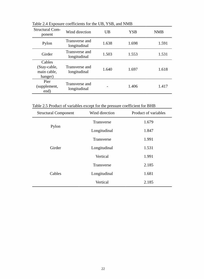
22

Table 2.4 Exposure coefficients for the UB, YSB, and NMB Structural Com-

ponent Wind direction UB YSB NMB

Pylon Transverse and longitudinal 1.638 1.698 1.591

Girder Transverse and longitudinal 1.503 1.553 1.531


hanger)

Transverse and longitudinal 1.640 1.697 1.618

Pier (supplement,

end)

Transverse and longitudinal - 1.406 1.417

Table 2.5 Product of variables except for the pressure coefficient for BHB

Structural Component Wind direction Product of variables

Pylon Transverse 1.679

Longitudinal 1.847

Girder

Transverse 1.991

Longitudinal 1.531

Vertical 1.991

Cables

Transverse 2.185

Longitudinal 1.681

Vertical 2.185

23

2.2 Probabilistic Description of Wind Velocity

The wind velocity in each design specification is designated as averaging wind ve-

locity in a certain period. The AASHTO specifications (AASHTO, 2014) adopts

3 seconds to average the wind velocity, which is referred to as the 3-s gust wind

velocity. Since, however, data averaged over a short time interval may prove as a

distorted picture of the intensity of the mean values (Simiu and Scanlan, 1999),

many design specifications adopts the averaging time of wind velocity longer than

3 seconds. Eurocode 1 (CEN, 2005) uses 1 hour averaged wind velocity, while

JRA (2007), CSA International (2000), KSCE (2006) and KMOLIT (2016a; 2016b)

utilize 10 minutes averaged wind velocity. The wind velocity for the five bridges

is averaged by every 10 minutes for constructing consistent statistical parameters,

as specified in KHBDC (LSD)-CB (KMOLIT, 2016b).

The 10 minutes-averaged wind velocities measured at the weather stations

nearest to the five cable-supported bridges are utilized to construct the probabilistic

model of wind velocity at the bridge site. The annual maximum wind velocities

are quoted from data in the homepage of Korea Meteorological Administration

(KMA, 2009), which provides wind data measured since 1964 or 1971 as presented

in Table 2.6. The terrain categories of each weather station are selected according

to the locations of the weather stations and are summarized in Table 2.6. Since

the Yeosu weather station moved in 1995, the changes in the terrain category are

considered in evaluating the annual maximum V10. The annual maximum V10 at

each bridge site is calculated using the formula given in Eq. (2.2). The mean and

standard deviation (SD) of the annual maximum V10 at each bridge site are calcu-

lated by the method of moments (Haldar and Mahadevan, 2000) and are presented

24

in Table 2.6. The wind velocity measured at the Yeosu weather station for the

YSB is modified using measure-correlate-predict algorithms (Rogers et al., 2005)

to take account for the wind environment of the site. The statistical parameters of

the annual maximum V10 measured at the Seoul and Ullengdo weather stations are

summarized for comparison purposes in Table 2.6. The statistical parameters of

wind velocity for the two regions are utilized to suggest the basic wind velocity for

KHBDC (LSD) (KMOLIT, 2016a) in Section 4.

The Kolmogorov-Smirnov goodness-of-fit test (Ang and Tang, 2007) is per-

formed with a significance level of 0.01 to confirm the distribution type of the an-

nual maximum V10 at each bridge site. The empirical CDF for the goodness-of-fit

test is constructed by the Weibull plotting positions (Cunnane, 1978) for obtaining

unbiased non-exceedance probabilities for all distributions. For the five bridges,

the normal, lognormal, Gumbel, Frechet, and Weibull distributions are not rejected

through the Kolmogorov-Smirnov goodness-of-fit tests as shown in Table 2.7. In

order to identify the most likelihood distribution type of wind velocity, the likeli-

hood functions are calculated for the five distribution types. The likelihood func-

tion, L, and the logarithm of the likelihood function are defined as follows.

);();();,,,( 1121 ϑϑ=ϑ XfXfXXXL XXn (2.5)

));(ln());(ln());,,,(ln( 121 ϑ++ϑ=ϑ nXXn XfXfXXXL (2.6)

where iX denotes the i-th data of a random variable, X, and ϑ indicates statisti-

cal parameters for an assumed distribution. )(Xf X presents the probability den-

sity function of the random variable, X. The mean and standard deviation of the

raw values of the annual maximum V10 are utilized as the statistical parameters of

25

the assumed distribution based on the method of moments (Haldar and Mahadevan,

2010). The values of the likelihood function and the logarithm of the function are

summarized in Table 2.7 for the NMB as a representative case for the five bridges.

The results of the goodness-of-ft tests and the values of likelihood functions for the

other four bridges exhibit similar patterns to those given in Table 2.7. As the

Gumbel distribution is the most likelihood distribution type among the tested five

distributions for the annual maximum V10, the distribution type of wind velocity is

defined as the Gumbel distribution in this study.

The cumulative distribution function (CDF) and the probability density func-

tion of the Gumbel distribution are expressed as follows:

))6

exp(exp()( γ−σ

µ−π−−=

X

XX

XXF (2.7)

)6

exp())6

exp(exp(16

)( γ−σ

µ−π−γ−

σµ−π

−−σ

π=

X

X

X

X

X

gbX

XXXf (2.8)

where )(XFX and )(Xf gbX indicate the CDF and probability density function of

the Gumbel distribution for a random variable X, and γ denotes Euler’s constant.

µX, σX, and δX represent the mean, the SD, and a coefficient of variation (COV) of

the variable X, respectively.

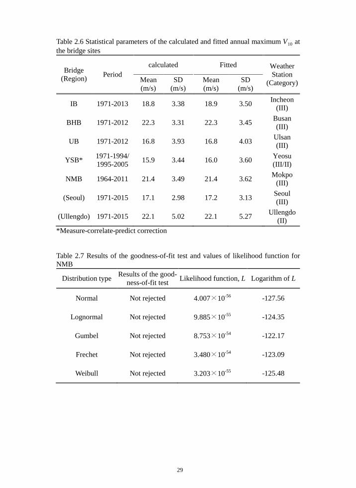
The statistical parameters of the fitted Gumbel distribution for the annual max-

imum V10 are calculated by the linear regression of the empirical CDF on the

Gumbel probability paper. In estimating the statistical parameters, the Gringorten

plotting positions optimized for the Gumbel distribution (Gringorten, 1963) are

adopted to construct the empirical CDF. The CDF obtained by the Weibull and

Gringorten positions are plotted with black and red centered symbols, respectively,

26

in Figs. 2.1-2.5 for five bridges.

The statistical parameters of a random variable fitted to the Gumbel distribu-

tion are obtained by a linear regression of cumulative probabilities on the probabil-

ity paper. The Gumbel probability paper is formed by plotting the logarithm of

the CDF. In the probability paper, the following linear relation between a random

variable, X, and the cumulative probability holds:

γ+σ

µ−π=−−

X

XX

XXF6

))(ln(ln( (2.9)

The cumulative probabilities of the Weibull and Gringorten plotting positions are

plotted on the Gumbel probability paper with centered symbols in Fig. 2.6- Fig.

2.10 for the five bridges. The data of the annual maximum V10 plotted on the

Gumbel probability paper shows linear trends. A straight line drawn through the

data points represents a specific Gumbel distribution for the annual maximum V10.

In Fig. 2.6- Fig. 2.10, the cumulative probabilities of the fitted Gumbel obtained by

the Weibull and Gringorten positions are plotted with the black and red lines on the

probability paper In Figs. 2.6-2.10.

As mentioned earlier, the Gringorten positions are optimized to the Gumbel

distribution, and thus the mean and SD of the fitted Gumbel distributions for the

annual maximum V10 are calculated based on the Gringorten plotting positions as

summarized in Table 2.6. The mean and SD of the 100- and 200-year maximum

V10 are obtained from those of the annual maximum V10 using the characteristics of

the Gumbel distribution and are given in Table 2.8. The theoretical CDFs calcu-

lated by the statistical parameters of the fitted Gumbel distribution for the annual

maximum V10 are illustrated in Figs 2.1-2.5. In the figures, the black and red

27

lines are corresponding to the Weibull and Gringorten plotting positions, respec-

tively.

Most reliability-based design codes define the nominal value of wind load us-

ing the wind velocity rather than the wind pressure, and the nominal value of V10 is

often referred to as a basic wind velocity. The basic wind velocity is generally

defined by the recurrence period of the wind velocity and the design life of a struc-

ture specified in the design code. The non-exceedance probability of the basic

wind velocity is equal to the probability of non-occurrence during the design life.

dt

V

VB

RV

)11())6

exp(exp(10

10 −=γ−σ

µ−π−− (2.10)

where VB, R and td denote the basic wind velocity, the recurrence period of the

wind velocity and the design life of a structure, respectively. The right-hand side

of Eq. (2.10) presents the probability of non-occurrence of the basic wind velocity

during the design life which is calculated based on Bernoulli process. For the sa-

ke of brevity in the forthcoming derivation, subscript V10 hereafter indicates V10

corresponding to the design life of td –year. If the recurrence period of the basic

wind velocity is presented as n times of the design life of a structure, Eq. (2.10) can

be written as follows.

nR

V

VB

RV

)11())6

exp(exp(10

10 −=γ−σ

µ−π−− (2.11)

As R is sufficiently large, the limit of the right-hand side of Eq. (2.11) approaches

(e-1/n).

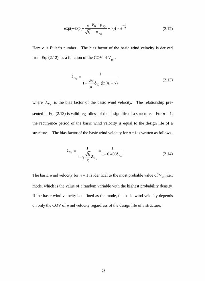
28

n

V

VB eV 1

))6

exp(exp(10

10−

≈γ−σ

µ−π−− (2.12)

Here e is Euler’s number. The bias factor of the basic wind velocity is derived

from Eq. (2.12), as a function of the COV of V10 .

))(ln(61

1

10γ−δ

π+

=λnV

VB

(2.13)

where BVλ is the bias factor of the basic wind velocity. The relationship pre-

sented in Eq. (2.13) is valid regardless of the design life of a structure. For n = 1,

the recurrence period of the basic wind velocity is equal to the design life of a

structure. The bias factor of the basic wind velocity for n =1 is written as follows.

1010

450.011

61

1

VV

VB δ−=

δπ

γ−=λ

(2.14)

The basic wind velocity for n = 1 is identical to the most probable value of V10, i.e.,

mode, which is the value of a random variable with the highest probability density.

If the basic wind velocity is defined as the mode, the basic wind velocity depends

on only the COV of wind velocity regardless of the design life of a structure.

29

Table 2.6 Statistical parameters of the calculated and fitted annual maximum V10 at the bridge sites

Bridge (Region) Period

calculated Fitted Weather Station

(Category) Mean (m/s)

SD (m/s) Mean

(m/s) SD

(m/s)

IB 1971-2013 18.8 3.38 18.9 3.50 Incheon (III)

BHB 1971-2012 22.3 3.31 22.3 3.45 Busan (III)

UB 1971-2012 16.8 3.93 16.8 4.03 Ulsan (III)

YSB* 1971-1994/ 1995-2005 15.9 3.44 16.0 3.60 Yeosu

(III/II)

NMB 1964-2011 21.4 3.49 21.4 3.62 Mokpo (III)

(Seoul) 1971-2015 17.1 2.98 17.2 3.13 Seoul (III)

(Ullengdo) 1971-2015 22.1 5.02 22.1 5.27 Ullengdo (II)

*Measure-correlate-predict correction

Table 2.7 Results of the goodness-of-fit test and values of likelihood function for NMB

Distribution type Results of the good-ness-of-fit test Likelihood function, L Logarithm of L

Normal Not rejected 4.007×10-56 -127.56

Lognormal Not rejected 9.885×10-55 -124.35

Gumbel Not rejected 8.753×10-54 -122.17

Frechet Not rejected 3.480×10-54 -123.09

Weibull Not rejected 3.203×10-55 -125.48

30

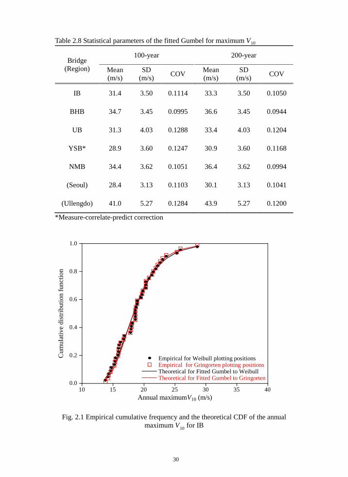
Table 2.8 Statistical parameters of the fitted Gumbel for maximum V10

Bridge (Region)

100-year 200-year

Mean (m/s)

SD (m/s) COV Mean

(m/s) SD

(m/s) COV

IB 31.4 3.50 0.1114 33.3 3.50 0.1050

BHB 34.7 3.45 0.0995 36.6 3.45 0.0944

UB 31.3 4.03 0.1288 33.4 4.03 0.1204

YSB* 28.9 3.60 0.1247 30.9 3.60 0.1168

NMB 34.4 3.62 0.1051 36.4 3.62 0.0994

(Seoul) 28.4 3.13 0.1103 30.1 3.13 0.1041

(Ullengdo) 41.0 5.27 0.1284 43.9 5.27 0.1200

*Measure-correlate-predict correction

0.0

0.2

0.4

0.6

0.8

1.0

10 15 20 25 30 35 40

Empirical for Weibull plotting positionsEmpirical for Gringorten plotting positionsTheoretical for Fitted Gumbel to WeibullTheoretical for Fitted Gumbel to Gringorten

Cum

ulat

ive

dist

ribut

ion

func

tion

Annual maximum V10 (m/s)

Fig. 2.1 Empirical cumulative frequency and the theoretical CDF of the annual maximum V10 for IB

31

0.0

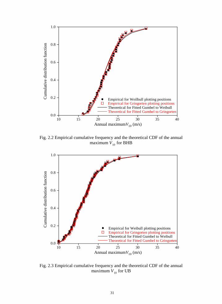
0.2

0.4

0.6

0.8

1.0

10 15 20 25 30 35 40

Empirical for Weilbull plotting positionsEmpirical for Gringorten plotting positionsTheoretical for Fitted Gumbel to WeibullTheoretical for Fitted Gumbel to Gringorten

Cum

ulat

ive

distr

ibut

ion

func

tion



maximum V10 for BHB

0.0

0.2

0.4

0.6

0.8

1.0

10 15 20 25 30 35 40


Cum

ulat

ive

distr

ibut

ion

func

tion



maximum V10 for UB

32

0.0

0.2

0.4

0.6

0.8

1.0

10 15 20 25 30 35 40

Empirical for Weibull plotting positionsEmpirical for Gringorten plotting positionsTheoretical for Fitted Gumbel to WeibullTheoretical for Fitted Gumbel to Weibull

Cum

ulat

ive

distr

ibut

ion

func

tion



maximum V10 for YSB

0.0

0.2

0.4

0.6

0.8

1.0

10 15 20 25 30 35 40


Cum

ulat

ive

distr

ibut

ion

func

tion



maximum V10 for NMB

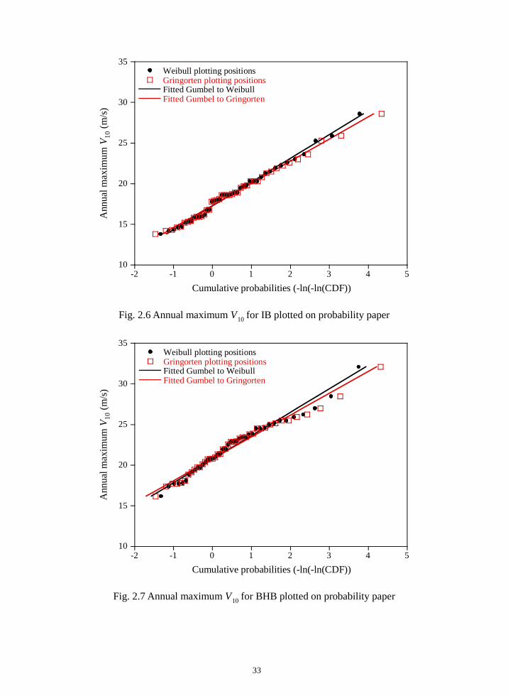
33

10

15

20

25

30

35

-2 -1 0 1 2 3 4 5

Weibull plotting positionsGringorten plotting positionsFitted Gumbel to WeibullFitted Gumbel to Gringorten

Ann

ual m

axim

um V

10 (m

/s)

Cumulative probabilities (-ln(-ln(CDF))

Fig. 2.6 Annual maximum V10 for IB plotted on probability paper

10

15

20

25

30

35

-2 -1 0 1 2 3 4 5


Ann

ual m

axim

um V

10 (m

/s)


Fig. 2.7 Annual maximum V10 for BHB plotted on probability paper

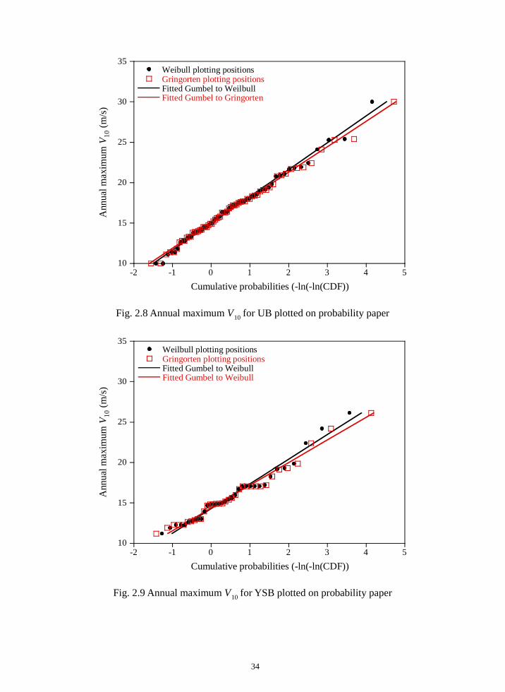
34

10

15

20

25

30

35

-2 -1 0 1 2 3 4 5

Weibull plotting positionsGringorten plotting positionsFitted Gumbel to WeilbullFitted Gumbel to Gringorten

Ann

ual m

axim

um V

10 (m

/s)


Fig. 2.8 Annual maximum V10 for UB plotted on probability paper

10

15

20

25

30

35

-2 -1 0 1 2 3 4 5

Weilbull plotting positionsGringorten plotting positionsFitted Gumbel to WeibullFitted Gumbel to Weibull

Ann

ual m

axim

um V

10 (m

/s)


Fig. 2.9 Annual maximum V10 for YSB plotted on probability paper

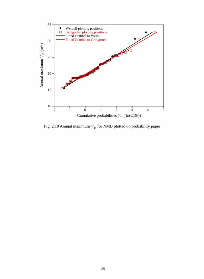
35

10

15

20

25

30

35

-2 -1 0 1 2 3 4 5


Ann

ual m

axim

um V

10 (m

/s)


Fig. 2.10 Annual maximum V10 for NMB plotted on probability paper

36

2.3 Probabilistic Description of Wind Pressure

The nominal value of wind load in a design specification is defined by using the

wind velocity, but the wind pressure is loaded on a structure to evaluate the wind

load effect generated in the structure. Therefore, the relationship between statisti-

cal parameters of the wind velocity and pressure should be identified to evaluate

the wind load factor based on the statistical parameters of the wind velocity. As

the magnitude of the wind pressure does not have an effect on the statistical rela-

tionships the wind pressure is normalized as follows.

WSZP

VGE

z

C

P

cVGECc

ZPZP

qVGECc

VGECc

GVEcCGVECWS

ZP

ZP

ˆ)ˆ(ˆˆˆˆ

)()(

21

210

2102

210

210air

10

10

µµ Ω=Ω=

µµµµµµµµµµ=

=ρ=

(2.15)

where WSq is normalized wind pressure, which is determined by the coefficients

and wind velocity normalized to their mean values. A random variable with a hat

indicates the variable normalized to its mean value. µΩ is a constant obtained by

multiplying the mean values of the coefficients to the mean wind velocity. Each

normalized variable has the mean value of 1, and the COV of the normalized varia-

bles becomes the COV of the original variables.

Monte-Carlo simulations are performed to construct a probabilistic model of

the normalized wind pressure. Table 2.9 presents the statistical parameters of the

coefficient for wind pressure. Since wind tunnel tests are performed for the de-

signs of cable-supported bridges, the COV of the pressure coefficient deduced by

Hong et al. (2009) is adopted in Monte-Carlo simulations while those of the analy-

37

sis coefficient and gust factor proposed by Ellingwood et al. (1980) are applied.

The COV of the exposure coefficient is also reduced as Hong et al. (2009) because

the wind environment is considered as Eq. (2.3) in the design of the cable-

supported bridges. The statistical model of the gust factor represents the uncer-

tainty of the wind pressure caused by the turbulence in wind and the wind-structure

interaction (Ellingwood et al., 1980).

The fitness of the normalized wind pressure obtained by Monte-Carlo simula-

tions to the four distributions such as lognormal, Gumbel, Frechet, Weibull distri-

butions is confirmed by the Kolmogorov-Smirnov goodness-of-fit test with a sig-

nificance level of 0.01. The empirical CDF is plotted by the Weibull plotting po-

sitions to confirm the distribution type. Table 2.10 shows the results of the good-

ness-of-fit tests for the NMB as the representative case of the five bridges. The

results of the goodness-of-fit tests for the other four bridges show same patterns as

those presented in Table 2.10. In the table, the critical values for the maximum

difference in the empirical and theoretical CDFs are summarized for given number

of simulations. Only the Gumbel distribution is not rejected for the smallest error

bound of the Kolmogorov-Smirnov goodness-of-fit test corresponding to 10 thou-

sand trials, and thus the Gumbel distribution is selected to define the theoretical

model for the wind pressure.

Monte-Carlo simulations with 100 million trials are performed to identify the

relationship between the statistical parameters of wind pressure and velocity. The

COV of the wind velocity for Monte-Carlo simulations varies from 0.08 to 0.16 at

intervals of 0.01. The statistical parameters of the fitted Gumbel distribution for

the normalized wind pressure are estimated by the linear regression of the cumula-

tive probabilities on the probability paper. The Gringorten plotting positions,

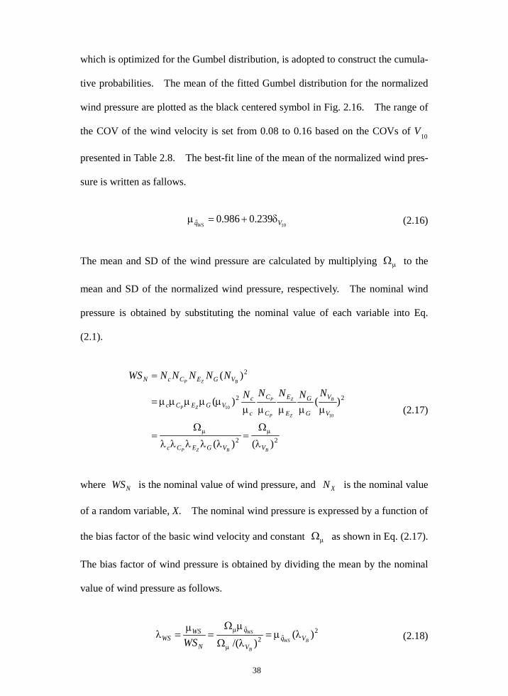
38

which is optimized for the Gumbel distribution, is adopted to construct the cumula-

tive probabilities. The mean of the fitted Gumbel distribution for the normalized

wind pressure are plotted as the black centered symbol in Fig. 2.16. The range of

the COV of the wind velocity is set from 0.08 to 0.16 based on the COVs of V10

presented in Table 2.8. The best-fit line of the mean of the normalized wind pres-

sure is written as fallows.

10239.0986.0ˆ VqWS

δ+=µ (2.16)

The mean and SD of the wind pressure are calculated by multiplying µΩ to the

mean and SD of the normalized wind pressure, respectively. The nominal wind

pressure is obtained by substituting the nominal value of each variable into Eq.

(2.1).

22

22

2

)()(

)()(

)(

10

10

BBZP

B

Z

Z

P

P

ZP

BZP

VVGECc

V

V

G

G

E

E

C

C

c

cVGECc

VGECcN

NNNNN

NNNNNWS

λ

Ω=

λλλλλ

Ω=

µµµµµµµµµµ=

=

µµ

(2.17)

where NWS is the nominal value of wind pressure, and XN is the nominal value

of a random variable, X. The nominal wind pressure is expressed by a function of

the bias factor of the basic wind velocity and constant µΩ as shown in Eq. (2.17).

The bias factor of wind pressure is obtained by dividing the mean by the nominal

value of wind pressure as follows.

2ˆ2

ˆ )()/( BWS

B

WSVq

V

q

N

WSWS WS

λµ=λΩ

µΩ=

µ=λ

µ

µ (2.18)

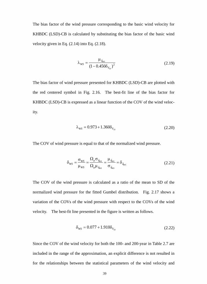
39

The bias factor of the wind pressure corresponding to the basic wind velocity for

KHBDC (LSD)-CB is calculated by substituting the bias factor of the basic wind

velocity given in Eq. (2.14) into Eq. (2.18).

2ˆ

)450.01(10V

qWS

WS

δ−

µ=λ (2.19)

The bias factor of wind pressure presented for KHBDC (LSD)-CB are plotted with

the red centered symbol in Fig. 2.16. The best-fit line of the bias factor for

KHBDC (LSD)-CB is expressed as a linear function of the COV of the wind veloc-

ity.

10360.1973.0 VWS δ+=λ (2.20)

The COV of wind pressure is equal to that of the normalized wind pressure.

WS

WS

WS

WS

WSq

q

q

q

q

WS

WSWS ˆ

ˆ

ˆ

ˆ

ˆ δ=σ

µ=

µΩ

σΩ=

µσ

=δµ

µ (2.21)

The COV of the wind pressure is calculated as a ratio of the mean to SD of the

normalized wind pressure for the fitted Gumbel distribution. Fig. 2.17 shows a

variation of the COVs of the wind pressure with respect to the COVs of the wind

velocity. The best-fit line presented in the figure is written as follows.

10

910.1077.0 VWS δ+=δ (2.22)

Since the COV of the wind velocity for both the 100- and 200-year in Table 2.7 are

included in the range of the approximation, an explicit difference is not resulted in

for the relationships between the statistical parameters of the wind velocity and

40

wind pressure. The relationships presented in Eqs. (2.20) and (2.22) are available

for KHBDC (LSD)-CB regardless of the design life of a structure.

In Fig. 2.12, the cumulative probabilities of the normalized wind pressure for

the NMB are plotted on the Gumbel probability paper as the representative case of

the five bridges. The black and red centered symbols indicate the Weibull and

Gringorten plotting positions, respectively, in the figure. Since the number of da-

ta generated by Monte-Carlo simulations is large enough, both the cumulative

probabilities of the two plotting positions appear very similar in the figures. It

should be noted that the results for the other bridges, which are not presented in

this work, exhibit similar patterns to those given in Fig. 2.12. In Fig.2.12, the re-

gression lines corresponding to each plotting position are drawn with the black and

red lines, respectively. The statistical parameters obtained by the Gringorten

plotting positions are selected as those of the fitted Gumbel distribution for the

normalized wind pressure. Table 2.11 shows the statistical parameters of the

normalized wind pressures and the square of the mean 10V for the five bridges.

`

Table 2.9 Statistical parameters of the coefficients in Eq. (2.1)

Random variable Bias factor COV (Ellingwood et al.)

COV (Hong et al.)

Distribution type

Analysis coefficient c 1.00 0.050 0.056 Normal

Pressure coefficient CP 1.00 0.160 0.075 Normal

Exposure coeffi-cient

Ez 1.00 0.120 0.075 Normal

Gust factor G 1.00 0.110 0.100 Normal

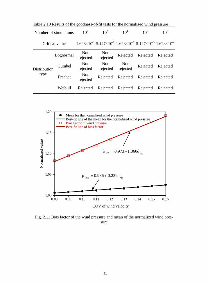
41

Table 2.10 Results of the goodness-of-fit tests for the normalized wind pressure

Number of simulations 102 103 104 105 108

Critical value 1.628×10-1 5.147×10-2 1.628×10-2 5.147×10-3 1.628×10-4

Distribution type

Lognormal Not rejected

Not rejected Rejected Rejected Rejected

Gumbel Not rejected

Not rejected

Not rejected Rejected Rejected

Frechet Not rejected Rejected Rejected Rejected Rejected

Weibull Rejected Rejected Rejected Rejected Rejected

1.00

1.05

1.10

1.15

1.20

0.08 0.09 0.10 0.11 0.12 0.13 0.14 0.15 0.16

Mean for the normalized wind pressureBest-fit line of the mean for the normalized wind pressureBias factor of wind pressureBest-fit line of bias factor

Nor

mal

ized

val

ue

COV of wind velocity

Fig. 2.11 Bias factor of the wind pressure and mean of the normalized wind pres-sure

10360.1973.0 VWS δ+=λ

10239.0986.0ˆ VqWS

δ+=µ

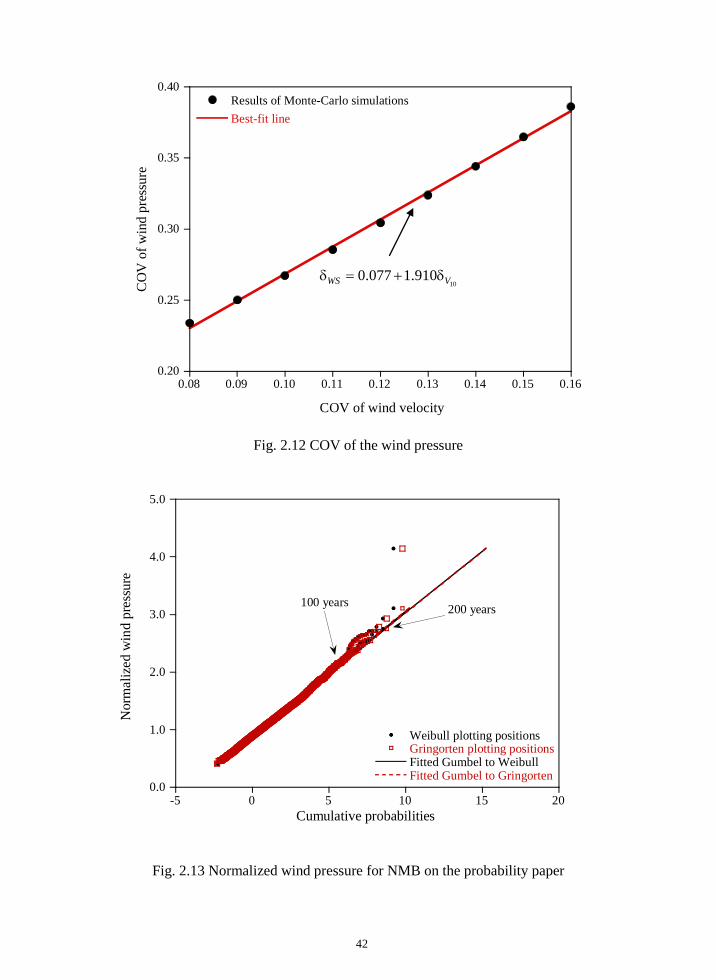
42

0.20

0.25

0.30

0.35

0.40

0.08 0.09 0.10 0.11 0.12 0.13 0.14 0.15 0.16

Results of Monte-Carlo simulationsBest-fit line

CO

V o

f win

d pr

essu

re


Fig. 2.12 COV of the wind pressure

0.0

1.0

2.0

3.0

4.0

5.0

-5 0 5 10 15 20


Nor

mal

ized

win

d pr

essu

re

200 years100 years

Cumulative probabilities

Fig. 2.13 Normalized wind pressure for NMB on the probability paper

10910.1077.0 VWS δ+=δ

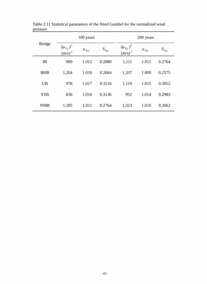
43

Table 2.11 Statistical parameters of the fitted Gumbel for the normalized wind pressure

Bridge 100 years

200 years

2)(10Vµ

(m/s) 2 WSqµ

WSqδ 2)(

10Vµ (m/s) 2

WSqµ WSqδ

IB 989 1.012 0.2880 1,111 1.011 0.2764

BHB 1,204 1.010 0.2664 1,337 1.009 0.2575

UB 978 1.017 0.3216 1,119 1.015 0.3052

YSB 836 1.016 0.3136 952 1.014 0.2983

NMB 1,185 1.011 0.2764 1,323 1.010 0.2662

44

SECTION 3

RELIABILITY ASSESSMENT OF RC COLUMNS

The important scope in code calibration is a development of a robust reliability as-

sessment method to calculate a reliability index accurately. Many studies

(Frangopol et al., 1996; Hong and Zhou, 1999; Jiang and Yang, 2013; Milner et al.,

2001 Mirza, 1996; Stewart and Attard, 1999; Szerszen et al., 2005) have been re-

ported for the reliability assessment of RC columns for uniaxial load using the

PMID, which defines the ultimate strength of an RC column. In the aforemen-

tioned studies, the strength of RC columns is defined as a specific point on the

PMID, and the studies required the time consuming Monte-Carlo simulations.

Recently, the authors and coworkers (Kim et al., 2015) proposed a new ap-

proach for the reliability assessment of RC columns subjected to uniaxial load,

which calculates the reliability index precisely without any assumption. It is

demonstrated that defining the strength of RC columns as a certain point on the

PMID results in erroneous solutions. The author and coworker also proposed a

robust reliability assessment method for RC columns subjected biaxial bending in

2017 (Kim and Lee, 2017). In this section, the details of the reliability assessment

methods suggested by the author and coworker are presented.

Section 3.1 introduces a reliability assessment method of RC columns subject-

ed to uniaxial bending based on the PMID using AFOSM (Haldar and Mahadevan,

2000). Section 3.2 presents an approach for the reliability assessment of RC col-

umns subjected to biaxial bending using the load contour method. The reliability

assessment of RC pylons for cable supported bridges are conducted in Section 3.3

45

3.1 Reliability Assessment of RC Columns Subjected to Uniaxial Bending Based on the P-M Interaction Diagram using AFOSM

Various studies (Frangopol et al., 1996; Hong and Zhou, 1999; Jiang and Yang,

2013; Milner et al., 2001 Mirza, 1996; Stewart and Attard, 1999; Szerszen et al.,

2005) suggested the reliability assessment method of RC columns subjected to uni-

axial bending. These studies are based on one common assumption that the

strength of an RC column can be pre-determined on the PMID by a load condition.

The strength of an RC column can be defined as a certain point of columns for spe-

cific eccentricities determined by load-path and load correlation of the axial force

to the bending moment (Frangopol et al., 1996; Hong and Zhou, 1999; Jiang and

Yang, 2013; Milner et al., 2001; Mirza, 1996; Stewart and Attard, 1999; Szerszen et

al., 2005). The aforementioned studies require time-consuming Monte-Carlo simu-

lations, and assume a certain relation between the bending moment and axial force.

The limit state function of an RC column is an approximation of a real limit state

function but a convenient form for applying a traditional reliability analysis scheme.

However, the approximated limit state function may lead to erroneous results be-

cause the real strength of an RC column at failure depends on not only the total

load effect but also the statistical characteristics of all random variables.

This section presents a new approach to estimate the MPFP and reliability in-

dex of an RC column under unixaixl bending based on the AFOSM (Haldar and

Mahadevan, 2000). Section 3.1.1 presents formulations of the AFOSM for the

PMID. In Section 3.1.2, the PMID of RC columns is approximated by using cu-

bic spline interpolation. Section 3.1.2 shows sensitivity calculations of the PMID

required in the AFOSM.

46

3.1.1 Formulation of the AFOSM for PMID

The PMID of an RC column subject to combined axial and flexural load is implic-

itly defined in the axial force (P)-moment (M) space as follows:

Ψ = Ψ(F, B) = 0 (3.1)

where TMP ),(=F , and B is the curve parameter vector of the PMID. The curve

parameters are determined based on the strength parameters representing the mate-

rial and geometric properties of a cross-section. The material properties include

the compressive strength of concrete, fck

, the Young’s modulus of the reinforcing

steel, Es, and the yield strength of the reinforcing steel, fy. A typical cross-section

of an RC column is illustrated in Fig. 3.1(a). The geometric properties consist of

the gross area of a cross-section as well as the area and position of each reinforcing

steel. The strength parameters of an RC column are conveniently written in one

vector.

(a) (b)

Fig. 3.1 Typical cross-section of an RC column: (a) definition of geometric proper-ties; and (b) variation of strain in a section.

εs,k

εcf

h Ag(ξ)

As,k

ys,k

py

ξ

y

47

Tmskssmskssgtsyckj yyyAAAAEffs ),,,,,,,,,,,,,()( ,,1,,,1, ==s (3.2)

where m, Agt, As,k, ys,k are the number of reinforcing steels, the gross area of a

cross-section, the area and position of the k-th reinforcing steel, respectively. The

position of reinforcing steel is measured from the extreme compression fiber of the

cross-section to the center of the reinforcing steel as shown in Fig. 3.1(a).

The PMID given in Eq. (3.1) defines the limit state of an RC column. That is,

Ψ(Fq, B) > 0 and Ψ(Fq, B) < 0 represent the safe and failure states of the RC col-

umn, respectively, and therefore Ψ(Fq, B) = 0 depicts the limit state of the RC col-

umn. Here, Fq is the internal force vector representing the load effects of external

load components such as dead load, live load, wind load, etc. Although each ex-

ternal load component may have nonlinear load effects on an RC column, linear

relations between the internal forces and the external loads are assumed in this

study:

qCF 0=

=

q

qq M

P (3.3)

Here, C0 and q are the load effect matrix and load parameter vector, respectively.

Each column of the load effect matrix is composed of the load effects calculated in

the structural analysis for the nominal value of the corresponding load component.

The load parameter vector represents the statistical parameters of the load compo-

nents. Each load parameter has the nominal value of 1, and its mean and COV

become the bias factor and the COV of the original load component, respectively.

The statistical distributions of the load parameters follow those of the original load

components. Although the load parameters are statistically independent, the in-

48

ternal forces become correlated to each other because they are expressed as the lin-

ear combinations of the same load parameters.

The strength parameters of an RC column and the load parameters are consid-

ered as random variables in this study. For the compactness of forthcoming deri-

vations, the random variables are written in one vector.

T),( sqX = (3.4)

Furthermore, all random variables are assumed to be normally distributed and stati-

cally independent to each other. The equivalent normal distributions estimated by

the Rackwitz-Fiessler method (Rackwitz and Fiessler, 1978) are utilized for

nonnormal distributed random variables.

The MPFP of an RC column is estimated using the probabilistic approach

based on the AFOSM, in which the MPFP is defined as the closest point on the

PMID from the origin in the standardized normal space of the random variables.

The MPFP of a column is given as the solution of the following minimization prob-

lem (Haldar and Mahadevan, 2000).

2

22Min X

X=β subject to 0)( =Ψ X (3.5)

where β and 2⋅ denote the reliability index and the 2-norm of a vector, respec-

tively, while the overbarred variables indicates standardized random variables and

)()( XX Ψ=Ψ . The MPFP in the standard normal space is calculated as follows

according to the geometric definition of the reliability index, which is the minimum

distance from the origin to the limit state in the standard normal space.

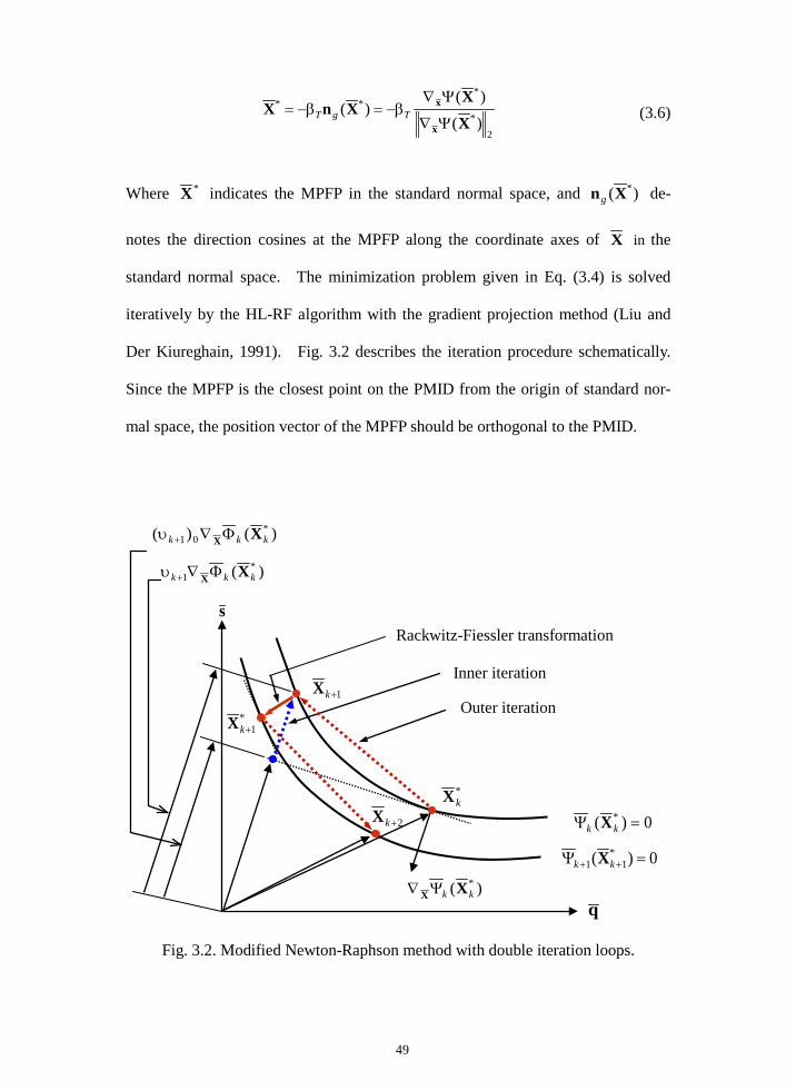
49

)(

)()(

2*

***

X

XXnX

x

x

Ψ∇

Ψ∇β−=β−= TgT (3.6)

Where *X indicates the MPFP in the standard normal space, and )( *Xng de-

notes the direction cosines at the MPFP along the coordinate axes of X in the

standard normal space. The minimization problem given in Eq. (3.4) is solved

iteratively by the HL-RF algorithm with the gradient projection method (Liu and

Der Kiureghain, 1991). Fig. 3.2 describes the iteration procedure schematically.

Since the MPFP is the closest point on the PMID from the origin of standard nor-

mal space, the position vector of the MPFP should be orthogonal to the PMID.

Fig. 3.2. Modified Newton-Raphson method with double iteration loops.

q

*kX

Inner iteration

2+kX

Outer iteration

)( *kk XXΨ∇

s

0)( *11 =Ψ ++ kk X

)( *1 kkk XX Φ∇υ +

)()( *01 kkk XX Φ∇υ +

0)( * =Ψ kk X

Rackwitz-Fiessler transformation

1+kX *

1+kX

50

)( ** XX XΦ∇υ−= (3.7)

where υ is an unknown scalar coefficient, and X∇ is the gradient operator with

respect to X . The first-order approximation of Eq. (3.7) is utilized for the New-

ton-Raphson method.

)(

.)H.O.T)()((

)(

*1

**2*1

*111

*1

kkk

kkkkk

kkkk

X

XXX

XX

X

XX

X

Ψ∇υ−≈

+∆Ψ∇+Ψ∇υ−=

Ψ∇υ−=

+

+

++++

(3.8)

where H.O.T. denotes higher order terms, subscript k is the iteration count and

Ψ∇2X

denotes the second-order sensitivity of the PMID with respect to the ran-

dom variables, which is difficult to evaluate and neglected in the approximation.

Since the second-order term is neglected in the approximation of the MPFP, the

iterational procedure based on Eq. (3.8) becomes the modified Newton-Raphson

method that is unable to exhibit the quadratic convergence rate (Conte and der

Boor, 1981).

The scalar unknown, 1+υk is determined using the PMID.

0))(( *

1 =Ψ∇υ−Ψ + kkkk XX (3.9)

As the PMID is nonlinear with respect to the MPFP, Eq. (3.9) becomes nonlinear

with respect to the scalar unknown, and another iteration procedure is required to

solve Eq. (3.9) for the scalar unknown within each iteration step of Eq. (3.8). The

scalar unknown is written in an incremental form:

υ∆+υ=υ +++ pkpk )()( 111 (3.10)

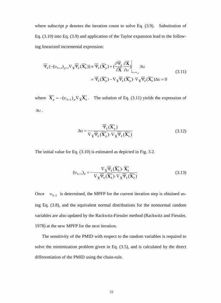
51

where subscript p denotes the iteration count to solve Eq. (3.9). Substitution of

Eq. (3.10) into Eq. (3.9) and application of the Taylor expansion lead to the follow-

ing linearized incremental expression:

0)()()(

)()())()((

***

**11

=υ∆Ψ∇⋅Ψ∇−Ψ=

υ∆υ∂

∂∂Ψ∂

+Ψ≈Ψ∇υ−Ψυ=υ

++

kkpkpk

kpkkkpkk

p

XXX

XX

XX

XX

X (3.11)

where *1

* )( kpkp XX X∇υ−= + . The solution of Eq. (3.11) yields the expression of

υ∆ .

)()()(

**

*

kkpk

pk

XXX

XX Ψ∇⋅Ψ∇

Ψ=υ∆ (3.12)

The initial value for Eq. (3.10) is estimated as depicted in Fig. 3.2.

)()()(

)( **

**

01kkkk

kkkk XX

XX

XX

X

Ψ∇⋅Ψ∇

⋅Ψ∇−=υ + (3.13)

Once 1+υk is determined, the MPFP for the current iteration step is obtained us-

ing Eq. (3.8), and the equivalent normal distributions for the nonnormal random

variables are also updated by the Rackwitz-Fiessler method (Rackwitz and Fiessler,

1978) at the new MPFP for the next iteration.

The sensitivity of the PMID with respect to the random variables is required to

solve the minimization problem given in Eq. (3.5), and is calculated by the direct

differentiation of the PMID using the chain-rule.

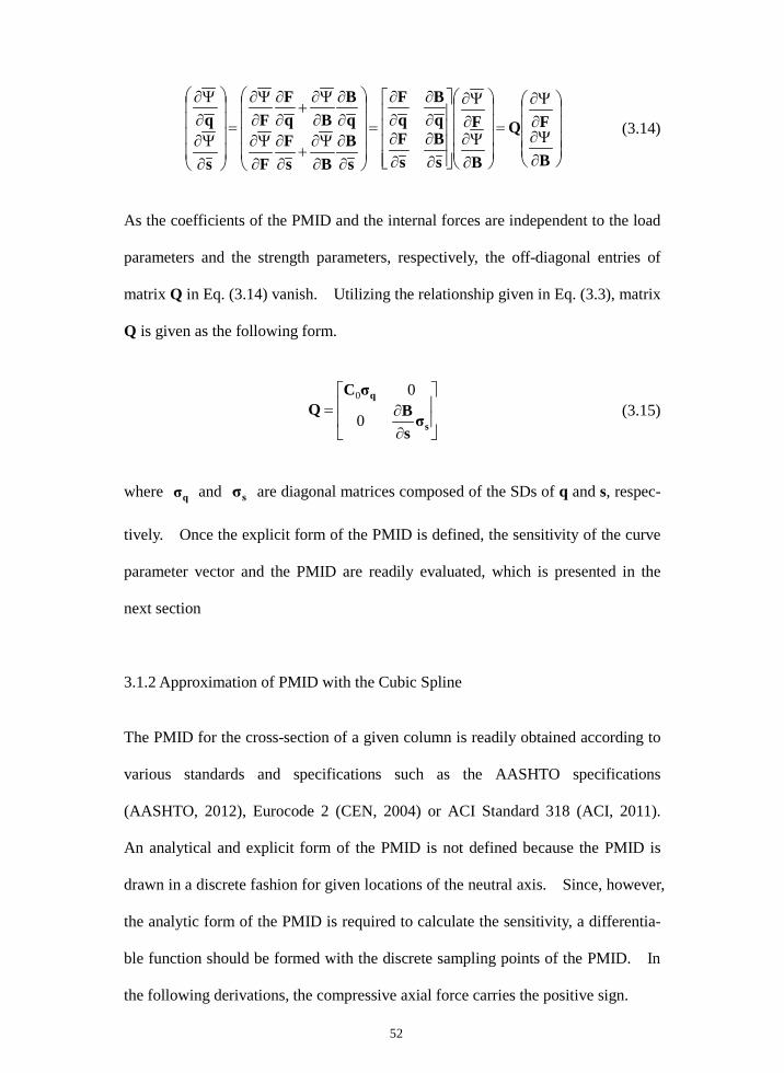
52

∂Ψ∂

∂Ψ∂

=

∂Ψ∂

∂Ψ∂

∂∂

∂∂

∂∂

∂∂

=

∂∂

∂Ψ∂

+∂∂

∂Ψ∂

∂∂

∂Ψ∂

+∂∂

∂Ψ∂

=

∂Ψ∂

∂Ψ∂

B

FQ

B

F

sB

sF

qB

qF

sB

BsF

F

qB

BqF

F

s

q (3.14)

As the coefficients of the PMID and the internal forces are independent to the load

parameters and the strength parameters, respectively, the off-diagonal entries of

matrix Q in Eq. (3.14) vanish. Utilizing the relationship given in Eq. (3.3), matrix

Q is given as the following form.

∂∂=

s

q

σsB

σCQ

0

00 (3.15)

where qσ and sσ are diagonal matrices composed of the SDs of q and s, respec-

tively. Once the explicit form of the PMID is defined, the sensitivity of the curve

parameter vector and the PMID are readily evaluated, which is presented in the

next section

3.1.2 Approximation of PMID with the Cubic Spline

The PMID for the cross-section of a given column is readily obtained according to

various standards and specifications such as the AASHTO specifications

(AASHTO, 2012), Eurocode 2 (CEN, 2004) or ACI Standard 318 (ACI, 2011).

An analytical and explicit form of the PMID is not defined because the PMID is

drawn in a discrete fashion for given locations of the neutral axis. Since, however,

the analytic form of the PMID is required to calculate the sensitivity, a differentia-

ble function should be formed with the discrete sampling points of the PMID. In

the following derivations, the compressive axial force carries the positive sign.

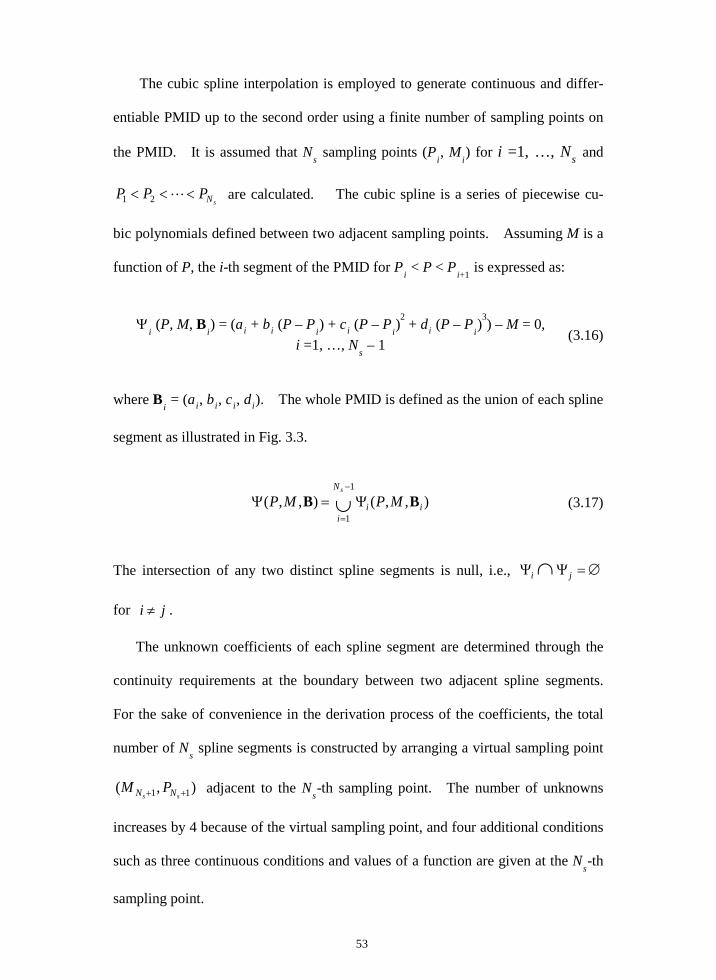
53

The cubic spline interpolation is employed to generate continuous and differ-

entiable PMID up to the second order using a finite number of sampling points on

the PMID. It is assumed that Ns sampling points (Pi, Mi) for i =1, …, Ns and

sNPPP <<< 21 are calculated. The cubic spline is a series of piecewise cu-

bic polynomials defined between two adjacent sampling points. Assuming M is a

function of P, the i-th segment of the PMID for Pi < P < Pi+1 is expressed as:

Ψ i (P, M, B i) = (ai + bi (P – Pi) + ci (P – Pi)

2 + di (P – Pi)3) – M = 0,

i =1, …, Ns – 1 (3.16)

where B i = (ai, bi, ci, di). The whole PMID is defined as the union of each spline

segment as illustrated in Fig. 3.3.

),,(),,(1

1ii

N

iMPMP

s

BB Ψ=Ψ ∪−

=

(3.17)

The intersection of any two distinct spline segments is null, i.e., ∅=ΨΨ ∩ ji

for ji ≠ .

The unknown coefficients of each spline segment are determined through the

continuity requirements at the boundary between two adjacent spline segments.

For the sake of convenience in the derivation process of the coefficients, the total

number of Ns spline segments is constructed by arranging a virtual sampling point

),( 11 ++ ss NN PM adjacent to the Ns-th sampling point. The number of unknowns

increases by 4 because of the virtual sampling point, and four additional conditions

such as three continuous conditions and values of a function are given at the Ns-th

sampling point.

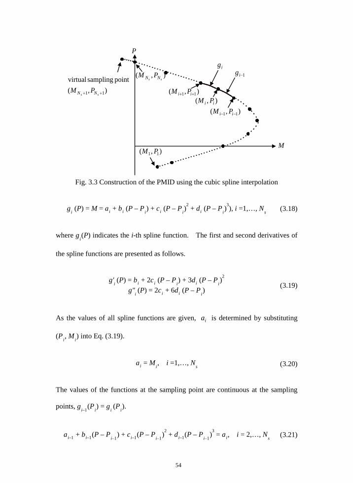
54

Fig. 3.3 Construction of the PMID using the cubic spline interpolation

gi (P) = M = ai + bi (P – Pi) + ci (P – Pi)

2 + di (P – Pi)3), i =1,…, Ns (3.18)

where gi(P) indicates the i-th spline function. The first and second derivatives of

the spline functions are presented as follows.

g'i (P) = bi + 2ci (P – Pi) + 3di (P – Pi)

2 g"i (P) = 2ci + 6di (P – Pi)

(3.19)

As the values of all spline functions are given, ia is determined by substituting

(Pi, Mi) into Eq. (3.19).

ai = Mi, i =1,…, Ns (3.20)

The values of the functions at the sampling point are continuous at the sampling

points, gi–1(Pi) = gi (Pi).

ai–1 + bi–1(P – Pi–1) + ci–1(P – Pi–1)2 + di–1(P – Pi–1)3 = ai, i = 2,…, Ns (3.21)

),(ss NN PM

),( 11 PM

),( ii PM),( 11 −− ii PM

M

P

1−igig

),( 11 ++ ii PM),(point sampling virtual

11 ++ ss NN PM

55

Eq. (3.21) is written as follows where pi–1 = Pi – Pi–1.

2

11111

11 −−−−

−

−− −−

−= iiii

i

iii pdpc

paab , i = 2,…, Ns (3.22)

The first derivative of the functions is continuously defined at each sampling point,

g'i–1(Pi) = g'i (Pi).

bi–1 + 2ci–1pi–1 + 3di–1p2

i–1= bi, i = 2,…, Ns (3.23)

di–1 is obtained by the condition that the second derivatives are continuous at the

sampling points, g"i–1(Pi) = g"i (Pi).

1

11 3 −

−−

−=

i

iii p

ccd , i = 2,…, Ns (3.24)

bi–1 is presented in terms of ai and pi by combining Eqs. (3.22) and (3.24).

11

1

11 3

2−

−

−

−−

+−

−= i

ii

i

iii pcc

paab , i = 2,…, Ns (3.25)

By substituting Eqs. (3.24) and (3.25) into Eq. (3.23), the algebraic equation for ic

is presented as follows.

)(3)(21

111111

−

−++−−−

−−

−=+++

i

ii

i

iiiiiiiii p

aap

aacpcppcp , i = 2,…, Ns – 1 (3.26)

There are 4Ns – 2 of conditions, while 4Ns of coefficients should be determined.

Therefore, to solve Eq. (3.26), the boundary conditions of 01 ==sNcc , which are

derived from d2M / dP2 = 0 at

sNPPP ,1= , are imposed. The coefficients ci in

56

Eq. (3.26) are obtained by solving the following linear system of algebraic equa-

tions:

pc = r (3.27)

where )(31

11

−

−+ −−

−=

i

ii

i

iii p

MMp

MMm , and the entries of matrix p and vector m

are composed of pi and mi, respectively. As p is a tridiagonal matrix, the com-

putation effort to solve Eq. (3.27) is trivial (Conte and der Boor, 1981).

3.1.3 Sensitivity Calculation

In case the current estimate of the MPFP exists in spline segment i, then the sensi-

tivities of the PMID are obtained by the direct differentiation of Eq. (3.16).

−−−

=∂Ψ∂

−−+−+

=∂Ψ∂

3

2

2

)()()(

1

, 1

)(3)(2

i

i

i

i

iiiiiii

PPPPPPPPdPPcb

BF (3.28)

The sensitivities of the curve parameter vector in matrix Q of Eq. (3.15) with re-

spect to the strength parameters are written as:

T

j

i

j

i

j

i

j

i

j

ii

sd

sc

sb

sa

s),,,(

∂∂

∂∂

∂∂

∂∂

=∂∂

=∂

∂ Bs

B for j = 1,…, Np (3.29)

where Np is the total number of the strength parameters. The sensitivities of coef-

ficients bi and di with respect to the strength parameters can be determined using

those of coefficients ai and ci. The sensitivity of coefficient ai simply becomes:

57

j

i

j

i

sM

sa

∂∂

=∂∂ for j = 1,…, Np (3.30)

The direct differential of Eq. (3.27) leads to the following expression:

)(1 cprpc

jjj sss ∂∂

−∂∂

=∂∂ − for j = 1,…, Np (3.31)

The above equation contains the sensitivities of matrix p and vector r, which are

given as:

))(

)(1

)()(1(3

12

1

11

1

211

1

j

i

i

ii

j

i

j

i

i

j

i

i

ii

j

i

j

i

ij

i

j

i

j

i

j

i

sp

pMM

sM

sM

p

sp

pMM

sM

sM

psr

sP

sP

sp

∂∂−

+∂

∂−

∂∂

−

∂∂−

−∂∂

−∂

∂=

∂∂

∂∂

−∂

∂=

∂∂

−

−

−−

−

++

+

for j = 1,…, Np (3.32)

The derivatives of ib and id are obtained by the direct differentiation of Eq.

(3.25) and Eq. (3.24), respectively.

j

i

i

ii

ij

i

j

i

j

i

j

iiii

j

i

j

i

j

i

i

ii

ij

i

j

i

j

i

sp

pcc

psc

sc

sd

spccp

sc

sc

sp

paa

psa

sa

sb

∂∂−

−∂∂

−∂

∂=

∂∂

∂∂+

−∂

∂+

∂∂

−

∂∂−

−∂∂

−∂

∂=

∂∂

++

++

++

211

11

211

)(311)(

31

32)2(

31

)(1)(

for j = 1,…, Np (3.33)

Eqs. (3.30), (3.32) and (3.33) contain the sensitivities of the sampling points with

respect to the strength parameters, i.e., ),(j

i

j

i

sM

sP

∂∂

∂∂

for i = 1,…, Ns and j = 1,…,

Np. These sensitivities are calculated directly utilizing the definition of the PMID.

58

The sampling point of a PMID corresponding to a given location of the neutral

axis of a cross-section is generally given as (Nilson et al., 2010):

∑∑∫

∑∑∫

∑∑∫

==ξ

==ξ

==ξ

σ−σ+σ−=

σ−+σ−−σ−=

σ+σ−σ=

m

kksksks

m

kkcksksA gcip

m

kksksksp

m

kkcksksp

Agcpi

m

kksks

m

kkcks

Agci

AyAydAyPy

AyyAyydAyyM

AAdAP

c

ig

c

ig

c

ig

1,,,

1,,,)(

1,,,

1,,,

)(

1,,

1,,

)(

)()()( (3.34)

where ξi, Ag(ξi), py , σc, σc,k and σs,k are the y-coordinate of the neutral axis of

the i-th sampling point, the gross area of the compressive region from the extreme

compression fiber to the neutral axis, the y-coordinate of plastic centroid, the com-

pressive stress of concrete, the compressive stress of concrete replacing the k-th

reinforcing steel and the stress of the k-th reinforcing steel, respectively, while mc

is the number of reinforcing steels in the compressive region. The gross area of

the compressive region is obtained by replacing reinforcing steels in the compres-

sive region with concrete. It is assumed in Eq. (3.34) that reinforcing steels of

iksy ξ≤, are in the compressive region, and that the stress of concrete replacing a

reinforcing steel is constant. Fig. 3.1(a) illustrates the definitions of the geometric

properties of a cross-section. The plastic centroid is given as follows (Nilson et

al., 2010):

stystgtcu

m

kksksy

m

kkskscucgtcu

p AfAA

yAfyAyAy

+−σ

+σ−σ=

∑∑==

)(1

,,1

,,

(3.35)

where Ast is the total cross-sectional area of the reinforcing steels, and cy is the y-

59

coordinate of the geometric centroid of the gross area of cross-section. σcu is the

stress of concrete corresponding to the ultimate compressive strain of concrete.

The stresses in concrete and reinforcing steels are determined through the

stress-strain curves of the corresponding materials. The stress of the k-th reinforc-

ing steel is obtained using the bilinear relation, which is not considered the strain

hardening of reinforcing steels, as shown in Fig. 3.4(a) (CEN, 2005).

ε≥εε<εε

=σspksy

spkskssks f

E

,

,,, for

for

(3.36)

where Es, εsp and εs,k are the Young’s modulus, the proportional limit of strain for

steel and the strain of the k-th reinforcing steel, respectively. As presented in

Eurocode 2 (CEN, 2004), one of three types of the stress-strain relations of con-

crete for the design of section may be utilized in the construction of the PMID: (1)

parabola-rectangle diagram; (2) bi-linear stress-strain relation; and (3) rectangular

stress distribution. The AASHTO specifications mainly adopts the third type

while the use of the first type is permitted (AASHTO, 2012). Since the second

and third types are simplified versions of the first one, the parabola-rectangle dia-

gram is employed for preciseness of analysis in this study. The parabola-

rectangle diagram is illustrated in Fig. 3.4(b) and defined as follows:

ε≤ε≤εγ

α

ε<ε≤εε−−γ

α

=σ22

22 0))/1(1(

cuccC

ckcc

ccn

ccC

ckcc

c f

f

(3.37)

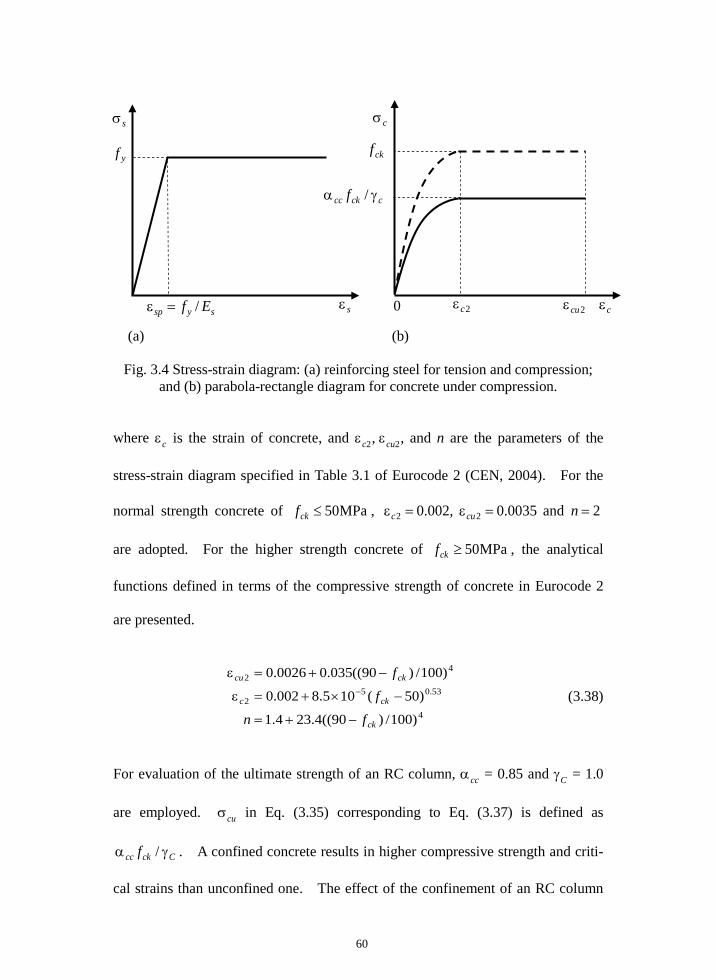
60

(a) (b)

Fig. 3.4 Stress-strain diagram: (a) reinforcing steel for tension and compression; and (b) parabola-rectangle diagram for concrete under compression.

where εc is the strain of concrete, and εc2, εcu2, and n are the parameters of the

stress-strain diagram specified in Table 3.1 of Eurocode 2 (CEN, 2004). For the

normal strength concrete of MPa50≤ckf , 2 and 0.0035 0.002, 22 ==ε=ε ncuc

are adopted. For the higher strength concrete of MPa50≥ckf , the analytical

functions defined in terms of the compressive strength of concrete in Eurocode 2

are presented.

4

53.052

42

)100/)90((4.234.1

)50(105.8002.0

)100/)90((035.00026.0

ck

ckc

ckcu

fn

f

f

−+=

−×+=ε

−+=ε− (3.38)

For evaluation of the ultimate strength of an RC column, αcc = 0.85 and γC = 1.0

are employed. σcu in Eq. (3.35) corresponding to Eq. (3.37) is defined as

Cckcc f γα / . A confined concrete results in higher compressive strength and criti-

cal strains than unconfined one. The effect of the confinement of an RC column

sysp Ef /=ε

sσ

yf

sε

cσ

ckf

cckcc f γα /

2cε 2cuε cε 0

61

on the strength is easily taken into account by adopting the stress-strain relation-

ships for the confined concrete given in the section 3.1.9 of Eurocode 2. KHBDC

(LSD) (KMOLIT, 2016a) also utilizes the bilinear relation and the parabola-

rectangle diagram to estimate the stress of reinforcing steels and concrete, respec-

tively. The stress-strain diagram of concrete and its parameters specified in

KHBDC (LSD) are briefly introduced in the APPENDIX A.

The strains of concrete and reinforcing steels are defined through purely geo-

metric consideration based on the Bernoulli’s beam theory. Since the cross-

section remains plane after deformation, the strain of concrete and reinforcing

steels is proportional to the distance from the extreme compression fiber to the neu-

tral axis. Reinforcing steels and concrete are completely attached to the integral

behavior. The tensile strength of concrete is ignored, and the effect of creep and

shrinkage is neglected. The strain varies linearly in the cross-section of a column

as shown in Fig. 3.1(b):

)()(

)( iyi

y cfi

cf ε+ξ

ε−=ε (3.39)

where )(yε indicates a strain of the cross-section at distance y from the extreme

compression fiber, and )(icfε denotes a strain at the extreme concrete compres-

sion fiber corresponding to the i-th neutral axis.

>ξ

εε−ε

−ξ

ξε≤ξ≤ε

=ε hh

h

i i

cu

ccui

ic

icu

cf for

0for

)(

2

22

2

2

(3.40)

Here, h denotes the depth of a cross-section.

62

The rectangular rule is adopted to evaluate the sampling point in Eq. (3.34)

numerically. The cross-section of a column is subdivided into Nl layers based

upon the discrete positions of the neutral axis, hlNi =ξ<<ξ<<ξ<ξ= 100 .

The positions of the neutral axis are sampled so that each layer has the same in-

cremental area of lgt NA / . The i-th layer indicates the gross area of the cross-

section between ξi–1 and ξi. Application of the rectangular rule to Eq. (3.34) leads

to the following expressions.

∑∑∑

∑

∑∑

∑∑∑

==

−

=++

=

=

−

=++

==

−

=+

σ−σ+σ−=

σ−+

σ−−σ−≈

σ+σ−σ≈

m

kksksks

m

kkcksks

i

kkck

gtip

m

kksksksp

m

kkcksksp

i

kkckp

gti

m

kksks

m

kkcks

i

kkc

gti

AyAyyNA

Py

Ayy

AyyyyNA

M

AANA

P

c

c

c

1,,,

1,,,

1

02/1,2/1

1,,,

1,,,

1

02/1,2/1

1,,

1,,

1

02/1,

)(

)()( (3.41)

Where )( ,, ksckc yσ=σ , )( 2/12/1, ++ σ=σ kckc y , 2/12/1 ++ ξ∆+ξ= kkky and

kkk ξ−ξ=ξ∆ ++ 11 . In this work, the sampling point on the PMID is not calculated

when the tensile stresses are generated throughout the cross-section. The sam-

pling points of the PMID is evaluated at each Nl neutral axes position except for ξ0

in which the neutral axis is located at the extreme concrete compression fiber.

As the neutral axis is positioned from the extreme tension fiber to infinity, the

strain at the extreme concrete compression fiber changes from εcu2 to εc2 as shown

in Eq. (3.40). The range of the strain at the extreme concrete compression fiber,

22 cucfc ε≤ε≤ε , is divided into No equal parts to determine the position of the neu-

tral axis located outside of the cross-section. The neutral axes are calculated ac-

63

cording to each εcf, and the sampling points corresponding to each neutral axis are

distributed at regular intervals on the PMID.

hk

k

ccf

cf

cu

ccuk

22

22

)()(ε−ε

ε

εε−ε

=ξ , o

ccucucf Nkk )()( 222 ε−ε−ε=ε

for oNk ≤≤1 (3.42)

The total number of sampling points constructing the PMID becomes Ns = Nl + No,

where Nl and No are applied as 100 and 20, respectively, in this study. In case the

neutral axis is positioned outside of the cross-section, the upper limits in the sum-

mations of the first terms in Eq. (3.41) should be taken as Nl – 1, i.e., i = Nl.

The direct differentiation of Eq. (3.41) with respect to the material properties of

an RC column leads to:

∑

∑

∑∑

=

=

=

−

=

+

∂

σ∂=

∂∂

=∂∂

∂σ∂

−∂

σ∂=

∂∂

m

k s

ksks

s

i

m

kkks

y

i

m

k ck

kcks

i

k ck

kcgt

ck

i

EA

EP

HAfP

fA

fNA

fP c

1

,,

1,

1

,,

1

0

2/1,

(3.43)

s

iks

s

ip

s

i

y

iksi

y

p

y

ip

y

i

m

k ck

kcksks

i

k ck

kck

l

gti

ck

p

ck

ip

ck

i

EPy

EPy

EM

fPyP

fy

fPy

fM

fAy

fy

NA

Pfy

fPy

fM c

∂∂

−∂∂

=∂∂

∂∂

−∂

∂+

∂∂

=∂∂

∂

σ∂+

∂

σ∂−

∂

∂+

∂∂

=∂∂ ∑∑

=

−

=

++

,

,

1

,,,

1

0

2/1,2/1

where

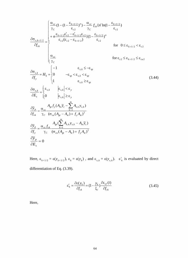
64

ε≤ε≤εγα

ε<ε≤ε

ε−

ε−εεεε′−ε′ε

+

εε

−′γα

−ε

ε−−

γα

=∂

σ∂

+

+

+

+

++

++

+

22/12

22/1

2

2/1

2/122

22/122/1

2

2/1

2

2/1

2/1,

for

0for

)1()(

)1ln())1(1(

cukcC

cc

ck

n

c

k

kcc

ckck

c

kck

C

ccn

c

k

C

cc

ck

kcn

nf

f

ε≥ε

ε<ε<ε−

ε−≤ε−

==∂σ∂

spks

spkssp

spks

ky

ks Hf

,

,

,,

1

0

1

ε≥ε

ε<εε=

∂σ∂

yks

yksks

s

ks

E ,

,,,

0

21

,,

))((

)(

stystgtcu

m

kkskscstygt

C

cc

ck

p

AfAA

yAyAfA

fy

+−σ

−

γα

=∂

∂ ∑=

21

,,

))((

)(

stystgtcu

cst

m

kksksgt

C

ckcc

y

p

AfAA

yAyAAf

fy

+−σ

−

γα

=∂

∂ ∑=

(3.44)

0=∂

∂

s

p

Ey

Here, εk+1/2 = ε(yk+1/2 ), εk = ε(yk ) , and εs ,k = ε(ys ,k ). ε'k is evaluated by direct

differentiation of Eq. (3.39).

ck

cf

i

k

ck

kk f

iyfy

∂ε∂

ξ−=

∂ε∂

=ε′)(

)1()( (3.45)

Here,

65

>ξ

∂ε∂

εξ

−+∂ε∂

εξε

ξ+ε

ξ−

≤ξ<∂ε∂

=∂

ε∂

h

fh

fh

hh

hf

fi

i

ck

ccu

ick

cuc

ic

icu

i

ick

cu

ck

cf

for

))1(())1((

1

0for

)( 222

222

222

2

(3.46)

n' , ε'c2 , and ε'cu2 are calculated by the direct differentiation method as follows.

34

47.0

52

2

322

)90(100

6.93)50(

10505.4

)100/)90(0014.0

ckck

ckck

cc

ckck

cucu

ffnn

ff

ff

−−=∂∂

=′

−×

=∂ε′∂

=ε′

−−=∂ε′∂

=ε′

−

(3.47)

Since the parameters of the stress-strain diagram for concrete in KHBDC (LSD)

differ from those presented in Eq. (3.38), the sensitivity of n' , ε'c2 , and ε'cu2 with

respect to the compressive strength of concrete is described in the APPENDIX A

individually.

The sensitivities of Eq. (3.41), with respect to the geometric properties become:

ls

lsls

m

kkl

ls

kcks

ls

i

ls

m

kklkc

ls

i

i

kkc

gt

i

yA

yA

yP

AP

NAP

c

c

,

,,

1 ,

,,

,

,1

,,

1

02/1,

1

∂σ∂

+δ∂σ∂

−=∂∂

σ+δσ−=∂∂

σ=∂∂

∑

∑

∑

=

=

−

=+

ljls

m

kklkcksi

ls

p

ks

ip

ls

i

gt

iki

gt

p

gt

ip

gt

i

yyPAy

APy

AM

APyP

Ay

APy

AM

c

,,1

,,,,,

2/1

σ−δσ+∂

∂+

∂∂

=∂∂

∂∂

−∂

∂+

∂∂

=∂∂

∑=

+

for ml ,,1=

(3.48)

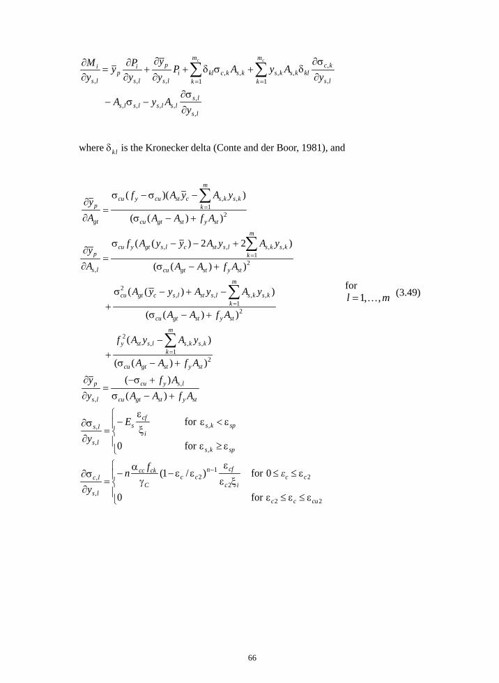
66

ls

lslslslsls

m

k ls

kcklksks

m

kkskckli

ls

p

ls

ip

ls

i

yAyA

yAyAP

yy

yPy

yM cc

,

,,,,,

1 ,

,,,

1,,

,,,

∂σ∂

−σ−

∂σ∂

δ+σδ+∂∂

+∂∂

=∂∂ ∑∑

==

where δkl is the Kronecker delta (Conte and der Boor, 1981), and

stystgtcu

lsycu

ls

p

stystgtcu

m

kkskslssty

stystgtcu

m

kkskslsstlscgtcu

stystgtcu

m

kkskslsstclsgtycu

ls

p

stystgtcu

m

kkskscstcuycu

gt

p

AfAAAf

yy

AfAA

yAyAf

AfAA

yAyAyyA

AfAA

yAyAyyAf

Ay

AfAA

yAyAf

Ay

+−σ

+σ−=

∂

∂

+−σ

−+

+−σ

−+−σ+

+−σ

+−−σ=

∂

∂

+−σ

−σ−σ=

∂

∂

∑

∑

∑

∑

=

=

=

=

)()(

))((

)(

))((

))((

))((

)22)((

))((

))((

,

,

21

,,,2

21

,,,,2

21

,,,,

,

21

,,

for ml ,,1= (3.49)

ε≤ε≤ε

ε≤≤ξε

εεε−

γα

−=

∂σ∂

ε≥ε

ε<εξε

−=

∂σ∂

−

22

22

12

,

,

,

,

,

,

for0

0for)/1(

for0

for

cucc

ccic

cfncc

C

ckcc

ls

lc

spks

spksi

cfs

ls

ls

εfny

Ey

67

3.2 Reliability Assessment of RC Columns Subjected to Biaxial Bending using the Load Contour Method

Various approaches for assessing the reliability of RC columns subjected to uniaxi-

al bending are available (Hong and Zhou, 1999; Szerszen et al., 2005; Jiang and

Yang, 2013; Kim et al., 2015). However, the reliability levels of RC columns sub-

jected to biaxial bending has been rarely reported except for one conference paper

(Wang and Hong, 2002) that showed a simplified approach based on the reciprocal

load method. The reliability levels of RC columns need to be evaluated accurate-

ly to determine a proper resistance factor and a target reliability index for various

limit states used in reliability-based code calibration.

In calculating the strength of RC columns, a basic assumption that a plane sec-

tion remains plane after deformation, is applicable to a section subjected to uniaxial

bending. However, the assumption is not valid in a plane section under biaxial

bending. Bresler (1960) proposed the load contour method, which estimates the

strength for biaxial bending by interpolation of the PMID for uniaxial bending

without the violation of the aforementioned assumption. The author and cowork-

er adopt the load contour method to define the strength of RC columns under biaxi-

al loads and proposed a robust reliability assessment method of RC columns for

biaxial loads using the load contour method (Kim and Lee, 2017). The load ef-

fects for each principal axis are superposed to implement for biaxial bending in the

reliability analysis.

In Section 3.2.1, the failure surface defined in the load contour method is pro-

vided as the limit state function for the reliability analysis. Section 3.2.2 presents

calculations for the sensitivity of the failure surface with respect to the random var-

iables required in the AFOSM.

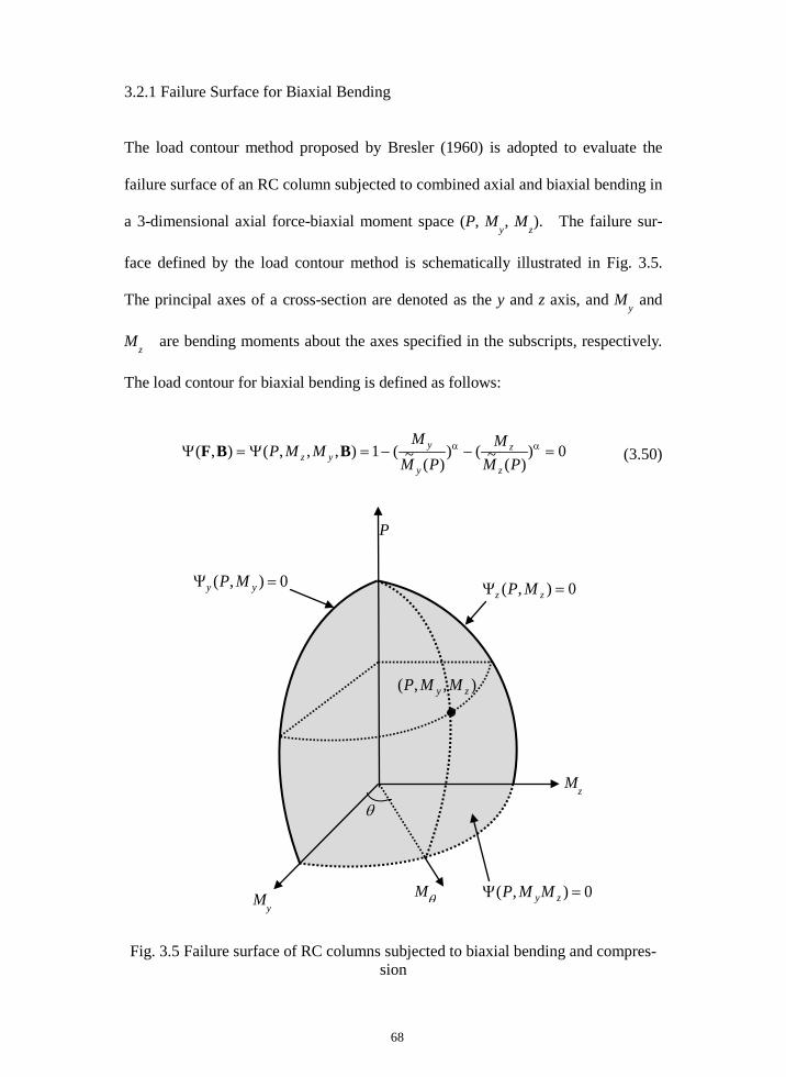
68

3.2.1 Failure Surface for Biaxial Bending

The load contour method proposed by Bresler (1960) is adopted to evaluate the

failure surface of an RC column subjected to combined axial and biaxial bending in

a 3-dimensional axial force-biaxial moment space (P, My, Mz). The failure sur-

face defined by the load contour method is schematically illustrated in Fig. 3.5.

The principal axes of a cross-section are denoted as the y and z axis, and My and

Mz are bending moments about the axes specified in the subscripts, respectively.

The load contour for biaxial bending is defined as follows:

0))(~()

)(~(1),,,(),( =−−=Ψ=Ψ αα

PMM

PMM

MMPz

z

y

yyz BBF (3.50)

Fig. 3.5 Failure surface of RC columns subjected to biaxial bending and compres-sion

My

Mz

P

Mθ

0),( =Ψ yy MP 0),( =Ψ zz MP

0),( =Ψ zyMMP

θ

),,( zy MMP

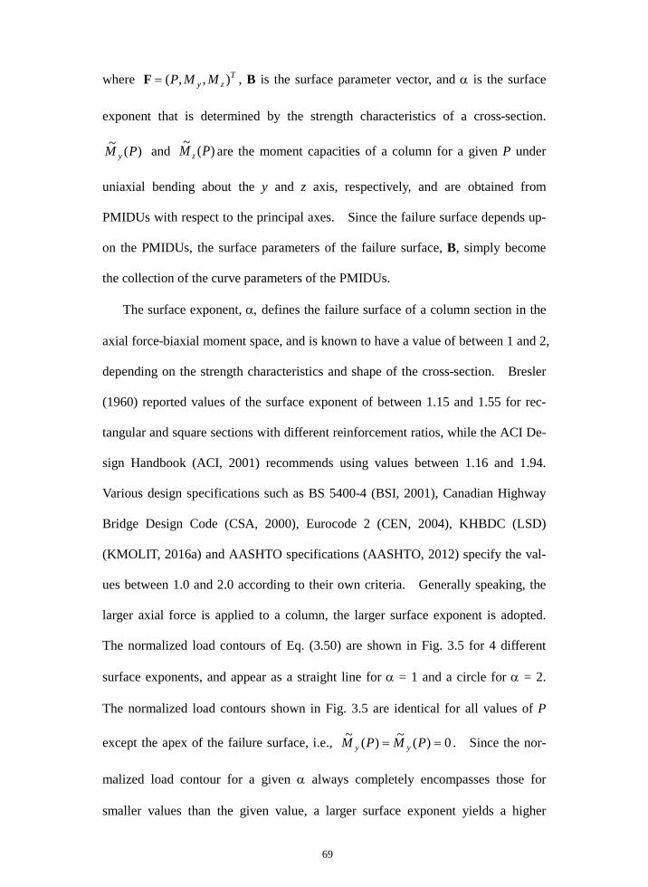
69

where Tzy MMP ),,(=F , B is the surface parameter vector, and α is the surface

exponent that is determined by the strength characteristics of a cross-section.

)(~ PM y and )(~ PM z are the moment capacities of a column for a given P under

uniaxial bending about the y and z axis, respectively, and are obtained from

PMIDUs with respect to the principal axes. Since the failure surface depends up-

on the PMIDUs, the surface parameters of the failure surface, B, simply become

the collection of the curve parameters of the PMIDUs.

The surface exponent, α, defines the failure surface of a column section in the

axial force-biaxial moment space, and is known to have a value of between 1 and 2,

depending on the strength characteristics and shape of the cross-section. Bresler

(1960) reported values of the surface exponent of between 1.15 and 1.55 for rec-

tangular and square sections with different reinforcement ratios, while the ACI De-

sign Handbook (ACI, 2001) recommends using values between 1.16 and 1.94.

Various design specifications such as BS 5400-4 (BSI, 2001), Canadian Highway

Bridge Design Code (CSA, 2000), Eurocode 2 (CEN, 2004), KHBDC (LSD)

(KMOLIT, 2016a) and AASHTO specifications (AASHTO, 2012) specify the val-

ues between 1.0 and 2.0 according to their own criteria. Generally speaking, the

larger axial force is applied to a column, the larger surface exponent is adopted.

The normalized load contours of Eq. (3.50) are shown in Fig. 3.5 for 4 different

surface exponents, and appear as a straight line for α = 1 and a circle for α = 2.

The normalized load contours shown in Fig. 3.5 are identical for all values of P

except the apex of the failure surface, i.e., 0)(~)(~== PMPM yy . Since the nor-

malized load contour for a given α always completely encompasses those for

smaller values than the given value, a larger surface exponent yields a higher

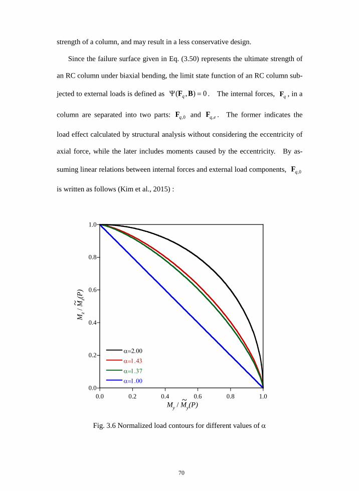
70

strength of a column, and may result in a less conservative design.

Since the failure surface given in Eq. (3.50) represents the ultimate strength of

an RC column under biaxial bending, the limit state function of an RC column sub-

jected to external loads is defined as 0),( =Ψ BFq . The internal forces, qF , in a

column are separated into two parts: 0,qF and eq,F . The former indicates the

load effect calculated by structural analysis without considering the eccentricity of

axial force, while the later includes moments caused by the eccentricity. By as-

suming linear relations between internal forces and external load components, 0,qF

is written as follows (Kim et al., 2015) :

Fig. 3.6 Normalized load contours for different values of α

0.0

0.2

0.4

0.6

0.8

1.0

0.0 0.2 0.4 0.6 0.8 1.0

α=2.00

α=1.43

α=1.37

α=1.00

Mz /

Mz(P

)

My / My(P)~

~

71

qCF 0

,

,0, =

=

zq

yq

q

q

M

M

P (3.51)

The moment in each direction induced by the corresponding eccentricity of axial

force is expressed as:

eqC

qCqCC0

qCqCF

−=

−=

−=

−=

=0

000 0 00

1,0

1,0

1,0

1.0

1,0

1,0

,

,,

y

z

y

zq

y

z

ze

yeeq

ee

eeP

ee

M

M (3.52)

where C0,1 is the first row vector of C0 in Eq. (3.51) while ey and ez denote the ec-

centricity in the direction of the y and z axis, respectively, and Tzy ee ),(=e is the

eccentricity vector. Two different forms of the internal force vector induced by

the eccentricity are given in terms of the load parameter and eccentricity vector in

Eq. (3.52) because the derivatives of the internal force vector with respect to both

the load parameter and eccentricity vector appear in the reliability analysis. For

the convenience of the forthcoming derivations, the two matrices in Eq. (3.52) are

denoted as follows:

−=

1,0

1,0

CC0

C

y

ze

ee and

−=

00

00~

1,0

1,0

qCqCCe (3.53)

The total load effect applied to a column is obtained by adding Eqs. (3.51) and

(3.52) together.

eCqCqCqCFFF eeeqqq

~00,0, +=+=+= (3.54)

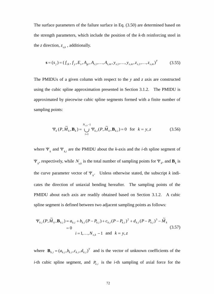
72

The surface parameters of the failure surface in Eq. (3.50) are determined based on

the strength parameters, which include the position of the k-th reinforcing steel in

the z direction, zs,k , additionally.

T

mssmssmssgtsyckj zzyyAAAEffs ),,,,,,,,,,,,()( ,1,,1,,1, ==s (3.55)

The PMIDUs of a given column with respect to the y and z axis are constructed

using the cubic spline approximation presented in Section 3.1.2. The PMIDU is

approximated by piecewise cubic spline segments formed with a finite number of

sampling points:

0),~,(),~,( ,,

1

1

,

=Ψ=Ψ ∪−

=ikkik

N

ikkk MPMP

ks

BB for zyk ,= (3.56)

where Ψk and Ψk,i are the PMIDU about the k-axis and the i-th spline segment of

Ψk, respectively, while Νs,k is the total number of sampling points for Ψk, and Bk is

the curve parameter vector of Ψk. Unless otherwise stated, the subscript k indi-

cates the direction of uniaxial bending hereafter. The sampling points of the

PMIDU about each axis are readily obtained based on Section 3.1.2. A cubic

spline segment is defined between two adjacent sampling points as follows:

0

~)()()(),~,( 3,,

2,,,,,,,

=

−−+−+−+=Ψ kikikikikikikikikkik MPPdPPcPPbaMP B

1,,1 , −= ksNi and zyk ,= (3.57)

where Tikikikikik dcba ),,,( ,,,,, =B and is the vector of unknown coefficients of the

i-th cubic spline segment, and ikP , is the i-th sampling of axial force for the

73

PMIDU in the P – Mk plane. The unknown coefficients of the cubic spline,

which are implicit functions of the strength parameters in Eq. (3.55), are deter-

mined using the continuity requirements up to the second order derivatives at the

boundary between two adjacent cubic spline segments. Detailed procedures for

constructing the PMIDU are given in Section 3.1.2.

3.2.2 AFOSM and Sensitivity

The strength parameters of an RC column, the load parameters and eccentricities of

the axial force are considered to be random variables, T),,( seqX = . All random

variables are assumed to be statistically independent of each other. In the case

where all random variables are normally distributed and statistically independent of

each other, the reliability index, β, and the corresponding MPFP are evaluated by

solving the minimization problem defined in the AFOSM. Since the limit state

function, i.e., the failure surface, is nonlinear with respect to the random variables,

the minimization problem can be solved iteratively using the HL-RF algorithm

with the gradient projection method (Liu and Der Kiureghain, 1991). The

Rackwitz-Fiessler method (Rackwitz and Fiessler, 1978) is adopted for nonnormal

random variables to estimate the equivalent normal distribution.

The sensitivity of the failure surface with respect to the random variables is re-

quired for the HL-RF algorithm. The direct differentiation of Eq. (3.50) with the

chain rule yields the sensitivity of the failure surface with respect to the standard-

ized random variables.

74

∂Ψ∂

∂Ψ∂

∂Ψ∂

=

∂Ψ∂

∂Ψ∂

∂Ψ∂

∂∂∂

∂

∂

∂∂

∂

∂∂∂∂

∂∂

∂

∂

∂∂

=

∂∂

∂Ψ∂

+∂

∂

∂Ψ∂

+∂∂

∂Ψ∂

∂∂

∂Ψ∂

+∂

∂

∂Ψ∂

+∂∂

∂Ψ∂

∂∂

∂Ψ∂

+∂

∂

∂Ψ∂

+∂∂

∂Ψ∂

=

∂Ψ∂

∂Ψ∂

∂Ψ∂

z

y

z

y

Tz

Tz

Ty

Ty

T

T

TzTyT

z

z

y

y

z

z

y

y

z

z

y

y

B

B

F

Q

B

B

F

sBe

B

sBe

B

sFeF

qB

qB

qF

sB

BsB

BsF

F

eB

BeB

BeF

F

qB

BqB

BqF

F

s

e

q

)(

)(

)(

)(

)(

)(

)()()(

(3.58)

The internal forces are related only with the load parameters and the eccentricities,

while the curve parameters of the PMIDUs depend only on the strength parameters.

Therefore, the sensitivities of the internal forces to the strength parameters as well

as those of the curve parameters to the load parameters and the eccentricities van-

ish in Eq. (3.58). Utilizing Eqs. (3.51) and (3.54), Q is written as follows.

∂∂

∂∂

+=

TzTTyT

Te

T

Te

TT

)

()

(0

00~00)( 0

sBσ

sB

σ

CσCCσ

Q

ss

e

q

(3.59)

where eσ is diagonal matrices composed of the SD of e. The sensitivities of the

curve parameters of the PMIDU in each direction to the strength parameters are

written as follows:

T

j

ik

j

ik

j

ik

j

ik

j

ikik

sd

sc

sb

sa

s),,,( ,,,,,,

∂∂

∂∂

∂∂

∂∂

=∂

∂=

∂∂ B

sB

for pNj ,,1= and zyk ,= (3.60)

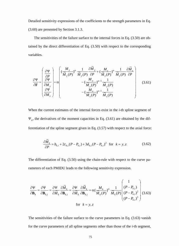
75

Detailed sensitivity expressions of the coefficients to the strength parameters in Eq.

(3.60) are presented by Section 3.1.3.

The sensitivities of the failure surface to the internal forces in Eq. (3.50) are ob-

tained by the direct differentiation of Eq. (3.50) with respect to the corresponding

variables.

)(~1)

)(~(

)(~1)

)(~(

~

)(~1)

)(~(~

)(~1)

)(~(

1

1

−

−

∂∂

+∂

∂

α=

∂Ψ∂

∂Ψ∂

∂Ψ∂

=∂Ψ∂

−α

−α

αα

PMPMM

PMPMM

PM

PMPMM

PM

PMPMM

M

M

P

zz

z

yy

y

z

zz

zy

yy

y

z

yF (3.61)

When the current estimates of the internal forces exist in the i-th spline segment of

Ψk, the derivatives of the moment capacities in Eq. (3.61) are obtained by the dif-

ferentiation of the spline segment given in Eq. (3.57) with respect to the axial force:

2

,,,,, )(3)(2~

ikikikikikk PPdPPcb

PM

−+−+=∂

∂ for zyk ,= (3.62)

The differentiation of Eq. (3.50) using the chain-rule with respect to the curve pa-

rameters of each PMIDU leads to the following sensitivity expression.

−−−

α=∂∂

∂Ψ∂

=∂∂

∂Ψ∂

=∂

Ψ∂=

∂Ψ∂ α

3,

2,

,

,,,

)()()(

1

)(~1)

)(~(~

~ ~

~

ik

ik

ik

kk

k

ik

k

kik

k

kikk

PPPPPP

PMPMMM

MM

M BBBB

for zyk ,=

(3.63)

The sensitivities of the failure surface to the curve parameters in Eq. (3.63) vanish

for the curve parameters of all spline segments other than those of the i-th segment,

76

because the failure surface for the current iteration is defined solely by the i-th

segment. Note that the spline segment used to evaluate Eqs. (3.61), (3.62) and

(3.63) may be a different segment for the individual PMIDU.

3.3 Reliability Assessment of RC Pylons for Cable-supported Bridges

The reliability analyses are performed for the design sections of RC pylons for two

cable-stayed and three suspension bridges presented in Section 2. Since the load

combination under a strong wind condition without the live load governs the de-

sign of the pylons, the dead and wind load effects are considered in the analyses.

The general view of the five cable-supported bridges and the longitudinal wind

direction (WD) are presented in Fig. 3.7. WD1 indicates the longitudinal wind

direction acting on the left pylon to the right pylon, and WD3 designates the oppo-

site wind direction of WD1. The front view of the pylons for the cable-supported

bridges is illustrated in Fig. 3.8. The transverse wind directions are indicated with

the arrows at the top of each pylon in the figure, and denoted as WD2 and WD4.

The transverse wind load is applied to both columns of a pylon simultaneously.

Each pylon consists of two symmetric columns, and the reliability analysis is con-

ducted for the bottom section of the left column for a pylon marked with a dotted

circle in Fig. 3.8.

The IB, which connects Young Jong Island to the city of Incheon, has been in

use since 2009. The total length of the cable-stayed bridge is 1,480m, and the

length of the longest span is 800m. 208 stay cables are located in the middle of

the bridge with a semi-fan system. The height of the pylons is 225.5m and its

shape looks like an inverted Y. The BHB is located in the North Port of Busan

77

and opened to the public in 2014. The total length of the cable-stayed bridge is

1,114m. The bridge has six traffic lanes with 28.7m wide. 80 stay cables with

semi-fan systems are anchored over two pylons symmetrically in the transverse and

longitudinal directions. The pylon is 190m high and is designed as a modified

diamond shape.

The UB is a single-span suspension bridge with two pylons, and was opened to

the public in 2015. The bridge crosses the Tae-hwa River in Ulsan Bay and ap-

proach viaducts of the bridge have different lengths. The total length of the

bridge and the length of the main span are 2,900m and 1,150m, respectively. The

H-type RC pylon is 203m high and 62 hangers are installed in the bridge. The

YSB is a typical suspension bridge which has three spans with two pylons, and

connects Yeosu to Gwangyang in Jeollanam-do. The YSB has been opened to the

public since 2012. The total length of the bridge is 2,260m and the longest span

length is 1,545m with 29.1m width. The number of hangers installed in the

bridge is 87. The pylon is a typical H-type pylon with height of 270m. The

NMB is a four-span suspension bridge with three pylons. The NMB is currently

under constructions and will be completed in 2018. The total length of the bridge

is 1,750m, and the length of two side spans and two middle spans are 225m and

650m, respectively. The number of hangers installed in NMB is 80. The design

of the middle pylon is governed by the gravitational-loads while the design for the

side pylons is governed by wind load. Therefore, the reliability assessment of the

pylon for the NMB is conducted using the cross-section of the side pylon at a

height of 151m.

Fig. 3.9 shows the geometry and arrangement of reinforcing steels of the cross-

section at the bottom of the pylons. As the cross-section of the pylons is a hollow

78

section, the section properties for internal forces have to be estimated based on the

effective flange width considering the shear lag or determined by rigorous analysis.

However, most design codes (AASHTO, 2012; KMOLIT, 2016a; KMOLIT, 2016b)

allow the full compression flange width effect for the capacity of a cross-section at

the strength limit state. The scope of this study is to determine the wind load fac-

tor of WGLS in the strength limit state, and thus the entire cross-section is valid to

evaluate the strength of RC pylons. Since the member axis of each column of the

pylons is inclined from the vertical line, the cross-sections shown in Fig. 3.9 are

projected to the plane perpendicular to the member axis and marked with a dotted

line in Fig. 3.8 for the reliability analysis. The inclined angle of the column and

sectional properties of the bottom sections of the pylons are summarized in Table

3.1. In the table, the nominal values of the compressive strength of concrete, the

yield strength, and Young’s modulus of the reinforcing steels are also presented.

The statistical parameters of the random variables are given in Table 3.2 and

quoted from the previous works (Kim et al., 2015; Nowak et al., 1994; Nowak,

1999; Nowak and Szerszen, 2003; Nowak and Eamon, 2008). DCP, DCG, DCC,

DW, and WS represent the dead load induced by the self-weights of the pylons,

girders, cable members, wearing surfaces and utilities, and the wind load, respec-

tively. The statistical variations of the reinforcing steel positions are defined with

the position errors in the examples.

ksksks yy ,,, ˆ η+= (3.56 )

where ksy ,ˆ and ks,η are the exact position and position error of the k-th reinforc-

ing steel, respectively. The normal distribution with zero mean is assumed for the

position error, and the radius of each reinforcing steel is taken as the SD. As the

79

mean of the position error is zero, the COV is not definable for the position error.

Table 3.3 presents the design VB which indicates the basic wind velocity used

in the actual design of the five cable-supported bridges, of which the design life is

100 years. The statistical parameters of the wind load are also given in the table.

The bias factor of the wind pressure corresponding to the design VB is obtained by

Eq. (2.18), and the COV of the wind pressure is calculated by Eq. (2.22). The

statistical parameters of the wind pressure are used for the wind load because the

statistical parameters of the wind pressure include analysis and model errors

(Ellingwood et al., 1980). Non-exceedance probability of wind load for the five

bridges varies from 06.46% to 98.72, which implies the different nominal wind

load is adapted to design of each bridge.

The actual load combinations adopted in design are employed for the reliability

analysis of the pylon section. The load effects induced by each load parameters

are calculated using a commercial program, and are presented in Tables 3.4 and 3.5

for the longitudinal and transverse directions, respectively. The calculated load

effects include a moment amplification effect due to the P-∆ effect. The load ef-

fects given in Tables 3.4 and 3.5 were used in the actual design of the five bridges.

In the tables, the compression depicts a positive sign. The positive bending mo-

ments for the longitudinal and transverse directions represent the clockwise action

in Fig. 3.7 and the counterclockwise action in Fig. 3.8, respectively. The WD in

parentheses of Tables 3.4 and 3.5 stands for the wind load direction illustrated in

Figs. 3.7 and 3.8. The load effect induced by the self-weights of stay-cables and

girders is not separated in the IB and the BHB because it is rather vague to calcu-

late their individual contributions to the load effect in cable-stayed bridges. The

actual wind pressure acting on a member is calculated by multiplying µΩ to the

80

normalized wind pressure as shown in Eq. (2.15).

The wind pressure is assumed to be uniformly distributed over a pylon with the

intensity evaluated at 65% of the pylon height for four bridges except for the IB.

The wind pressures for the IB are applied to the pylon with distributed values ac-

cording to the height. The wind pressure on the pylons is considered in both

transverse and longitudinal directions. In the other types of members, the wind

pressure is evaluated at the representative height of an individual member. The

wind pressures on a girder in the drag, lift, and rotational directions are calculated

by using corresponding pressure coefficients, and are applied on the girder in the

transverse direction for the four bridges except for the BHB. In the design of

BHB, the wind pressure in the rotational direction is not considered for girders.

In the longitudinal direction, only the drag action of wind is considered for the

girder by using 25% of the wind pressure. For the IB, BHB, and UB, the wind

pressures on the cable members are considered in both transverse and longitudinal

directions, while the wind pressures acting on the cable members in the longitudi-

nal direction are not taken into account in the design of YSB and NMB. The wind

pressures are applied to each bridge member of the bridges to estimate the wind

load effects.

The reliability analyses are performed for the transverse and longitudinal load

effects individually. The HL-RF algorithm with the gradient projection method is

utilized to calculate the reliability index and MPFP. In Fig. 3.10, the convergence

rates of the HL-RF algorithm with the gradient projection method are compared to

those of the HL-RF algorithm (Rackwitz-Fiessler, 1978), which is commonly used

in the reliability analysis. The figure shows the convergence rate obtained by the

reliability assessment of the pylon for YSB as the representative case of the five

81

bridges. Intermediate iterational solutions in the HL-RF algorithm with the gra-

dient projection method always satisfy the limit state function by virtue of inner

iterations, which causes much faster convergence rate compared to the HL-RF

method without gradient projection. The computational effort, of course, increas-

es for the HL-RF algorithm with the gradient projection method due to the inner

iterations, which may be compensated for the faster convergence rate. Table 3.6

shows the reliability indexes of the pylon sections for the five bridges. The min-

imum reliability indexes are calculated as 4.14 to 4.72 when the wind load acts on

a pylon in WD2 for the five bridges. The load effects in which the tensile force is

generated in a cross-section by the wind load govern the design of the pylon. The

results of the reliability analyses for the other wind load directions are discussed in

detail via BHB by Kim et al (2015), and are not presented in this thesis.

For the brevity of forthcoming discussions, the PMIDs corresponding to the

nominal and mean values of the strength parameters are referred to as the nominal

and mean PMID, respectively. The PMID drawn with the strength parameters at

the MPFP is referred to as the limit PMID. The points in the P–M space corre-

sponding to the load effects evaluated at the MPFP and the nominal values of the

external load parameters are called as the failure point and nominal load effect,

respectively. The limit PMID of each load combination in the following exam-

ples is presented to identify the failure mode of a column by investigating the rela-

tive location of the failure point on the limit PMID. Since the random variables at

the limit state obtained by the AFOSM satisfy the limit state function exactly, a

failure point always lies on a limit PMID. Physically, the limit PMID represents

the overall strength of an RC column at the limit state, and the failure point indi-

cates the load effect that yields the lowest reliability index on the limit PMID.

82

The results of the analyses for WD2 are presented in Table 3.7 and Figs. 3.11-

3.20. The random variables at the MPFP are normalized to their nominal values

in the table. Since it is difficult to present the position errors and cross-sectional

areas of all reinforcing steels at the MPFP, their average values are given in the

corresponding tables. The dead load parameters are calculated as roughly 1.1

times of the nominal values at the failure, and thus the moment amplification effect

due to the increase of axial forces may be neglected during the reliability analysis.

It should be noted that the geometric properties of reinforcing steels have little ef-

fect on the reliability index and corresponding MPFP.

The various types of PMIDs are shown in Fig. 3.11-3.15, along with the load

effect at the failure point for the five bridges. Since the normalized MPFPs of the

random variables except for the wind load are located nearby their mean values as

shown in Table 3.7, the mean and limit PMIDs in Figs. 3.11-3.15 are drawn very

close to one another. This is because the wind load follows an extreme type dis-

tribution with a large COV, which results in a dominant sensitivity of the limit state

function to the wind load in the AFOSM over the other variables. The effect of

the random variables on the failure of the pylon is investigated through reliability

analyses of the cross-section designed with various reinforcement ratios. The re-

liability indexes and the normalized MPFPs of the random variables with respect to

the reinforcement ratio of the cross-section are plotted for the five bridges in Figs

3.16 - 3.20. The variation patterns of the MPFP for the wind load and the reliabil-

ity index are quite similar to each other, which implies that the wind load governs

the failure of the column. The magnitude of the MPFPs of other variables is

maintained constant regardless of the reinforcement ratio, and thus the variables

rarely have an effect on the results of the reliability analysis.

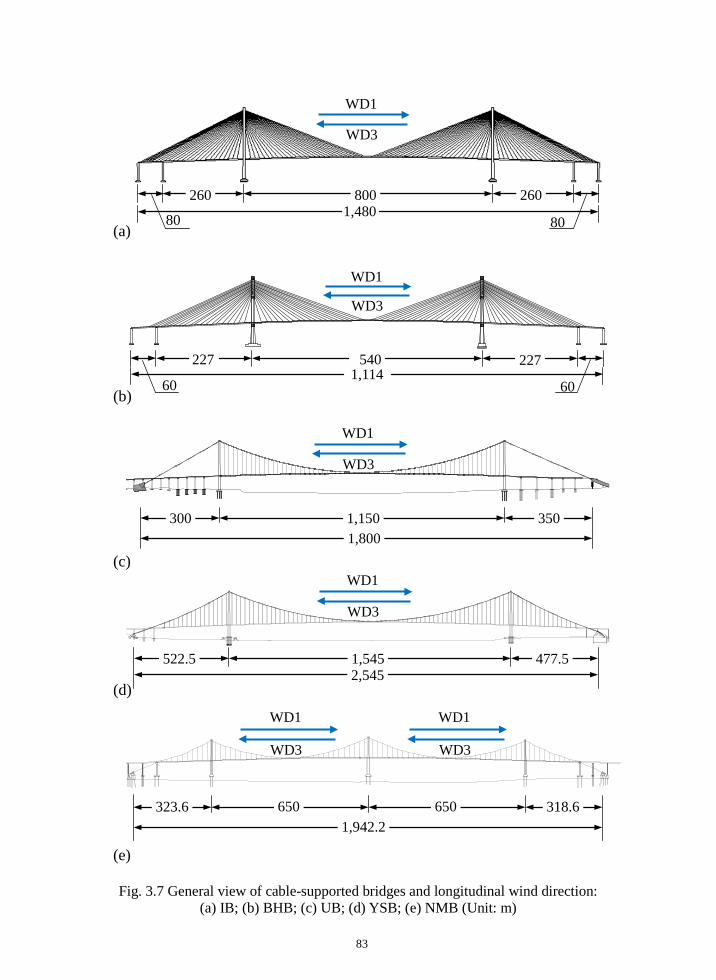
83

(a) (b) (c) (d) (e) Fig. 3.7 General view of cable-supported bridges and longitudinal wind direction:

(a) IB; (b) BHB; (c) UB; (d) YSB; (e) NMB (Unit: m)

60

227 540 1,114

227

60

WD1

WD3

1,800 300 1,150 350

WD1

WD3

318.6 650 650 1,942.2

323.6

WD1

WD3

WD1

WD3

2,545 522.5 1,545 477.5

WD1

WD3

260 800 260

80 80 1,480

WD1

WD3

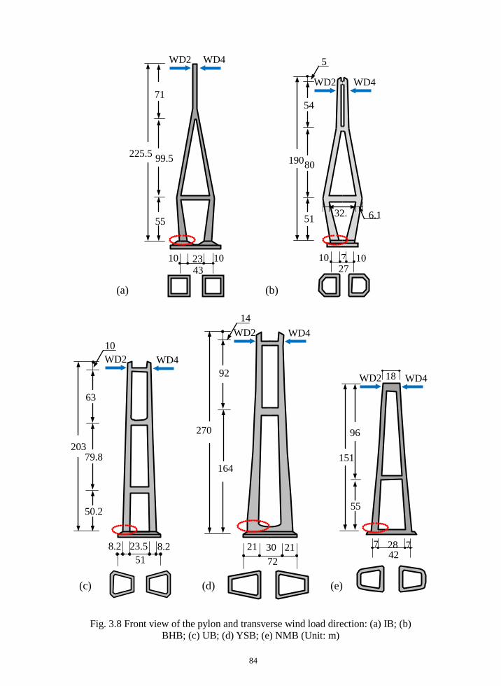
84

(a) (b)

(c) (d) (e)

Fig. 3.8 Front view of the pylon and transverse wind load direction: (a) IB; (b)

BHB; (c) UB; (d) YSB; (e) NMB (Unit: m)

225.5 99.5

55

71

43 10 23 10

WD2 WD4

WD2 WD4

203

50.2

63

10

51 23.5 8.2 8.2

79.8

WD2 WD4

270

164

92

14

72 21 30 21

151

96

55

18

42 7 28 7

WD2 WD4

WD2 WD4

27 10 7 10

32.

6.1

5

190 80

51

54

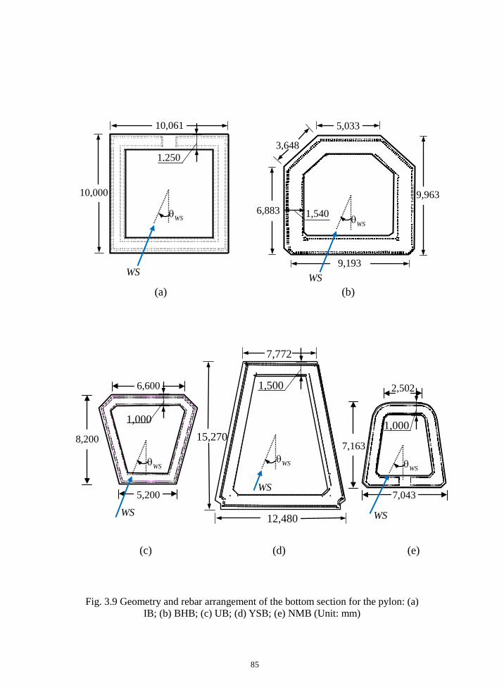
85

(a) (b)

(c) (d) (e)

Fig. 3.9 Geometry and rebar arrangement of the bottom section for the pylon: (a)

IB; (b) BHB; (c) UB; (d) YSB; (e) NMB (Unit: mm)

10,061

10,000

1,250

9,963

9,193

1,540

5,033

3,648

6,883

8,200

5,200

6,600

1,000 15,270

1,500

12,480

7,772

1,000

7,043

7,163

2,502

WS

θWS

WS

θWS

WS

θWS

WS

θWS

WS

θWS

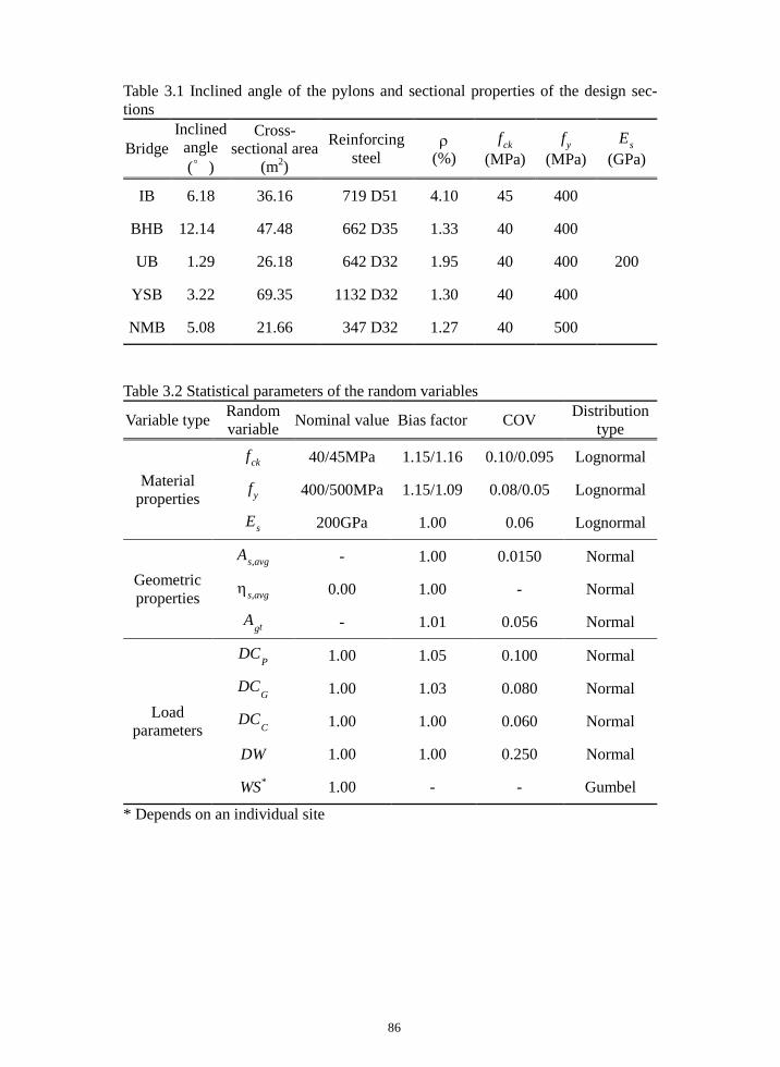
86

Table 3.1 Inclined angle of the pylons and sectional properties of the design sec-tions

Bridge Inclined

angle (°)

Cross-sectional area

(m2)

Reinforcing steel

ρ (%)

fck (MPa)

fy (MPa)

Es (GPa)

IB 6.18 36.16 719 D51 4.10 45 400

200

BHB 12.14 47.48 662 D35 1.33 40 400

UB 1.29 26.18 642 D32 1.95 40 400

YSB 3.22 69.35 1132 D32 1.30 40 400

NMB 5.08 21.66 347 D32 1.27 40 500

Table 3.2 Statistical parameters of the random variables

Variable type Random variable Nominal value Bias factor COV Distribution

type

Material properties

fck 40/45MPa 1.15/1.16 0.10/0.095 Lognormal

fy 400/500MPa 1.15/1.09 0.08/0.05 Lognormal

Es 200GPa 1.00 0.06 Lognormal

Geometric properties

As,avg - 1.00 0.0150 Normal

ηs,avg 0.00 1.00 - Normal

Agt - 1.01 0.056 Normal

Load parameters

DCP 1.00 1.05 0.100 Normal

DCG 1.00 1.03 0.080 Normal

DCC 1.00 1.00 0.060 Normal

DW 1.00 1.00 0.250 Normal

WS* 1.00 - - Gumbel

* Depends on an individual site

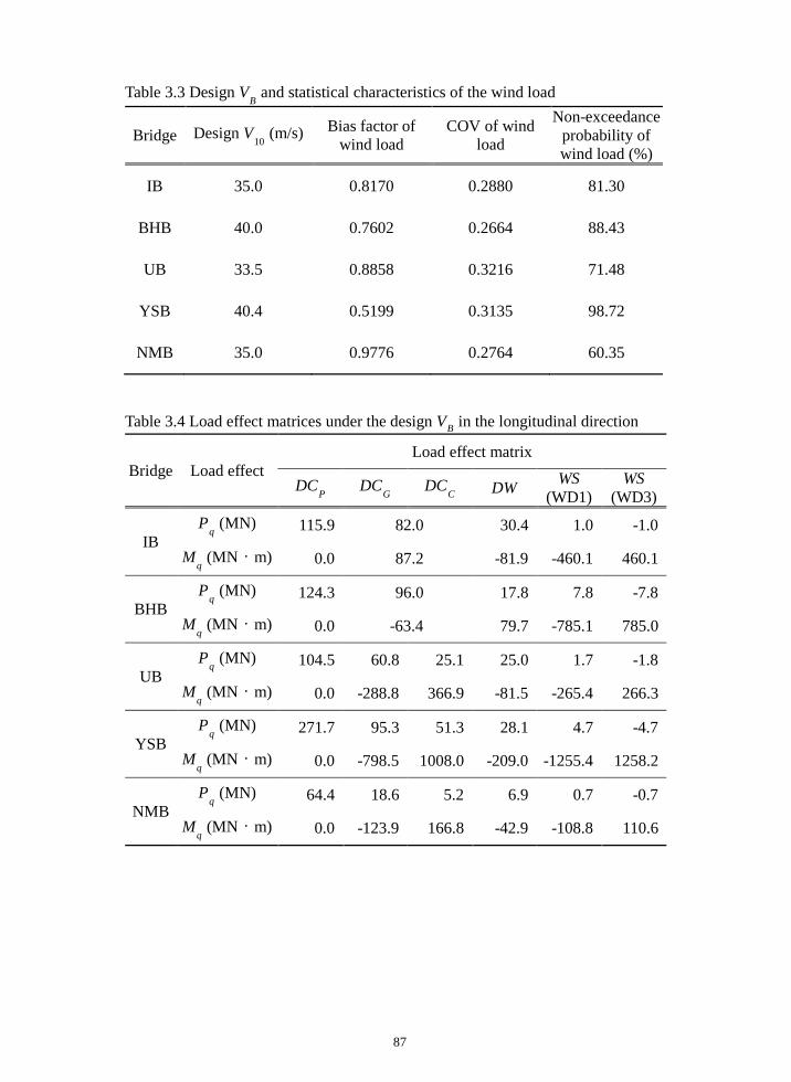
87

Table 3.3 Design VB and statistical characteristics of the wind load

Bridge Design V10 (m/s) Bias factor of wind load

COV of wind load

Non-exceedance probability of wind load (%)

IB 35.0 0.8170 0.2880 81.30

BHB 40.0 0.7602 0.2664 88.43

UB 33.5 0.8858 0.3216 71.48

YSB 40.4 0.5199 0.3135 98.72

NMB 35.0 0.9776 0.2764 60.35

Table 3.4 Load effect matrices under the design VB in the longitudinal direction

Bridge Load effect Load effect matrix

DCP DCG DCC DW WS

(WD1) WS

(WD3)

IB Pq (MN) 115.9 82.0 30.4 1.0 -1.0

Mq (MN·m) 0.0 87.2 -81.9 -460.1 460.1

BHB Pq (MN) 124.3 96.0 17.8 7.8 -7.8

Mq (MN·m) 0.0 -63.4 79.7 -785.1 785.0

UB Pq (MN) 104.5 60.8 25.1 25.0 1.7 -1.8

Mq (MN·m) 0.0 -288.8 366.9 -81.5 -265.4 266.3

YSB Pq (MN) 271.7 95.3 51.3 28.1 4.7 -4.7

Mq (MN·m) 0.0 -798.5 1008.0 -209.0 -1255.4 1258.2

NMB Pq (MN) 64.4 18.6 5.2 6.9 0.7 -0.7

Mq (MN·m) 0.0 -123.9 166.8 -42.9 -108.8 110.6

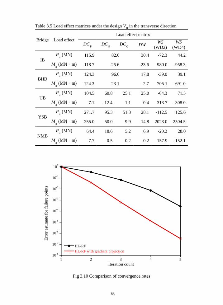
88

Table 3.5 Load effect matrices under the design VB in the transverse direction


DCP DCG DCC DW WS

(WD2) WS

(WD4)

IB Pq (MN) 115.9 82.0 30.4 -72.3 44.2

Mq (MN·m) -118.7 -25.6 -23.6 980.0 -958.3

BHB Pq (MN) 124.3 96.0 17.8 -39.0 39.1

Mq (MN·m) -124.3 -23.1 -2.7 705.1 -691.0

UB Pq (MN) 104.5 60.8 25.1 25.0 -64.3 71.5

Mq (MN·m) -7.1 -12.4 1.1 -0.4 313.7 -308.0

YSB Pq (MN) 271.7 95.3 51.3 28.1 -112.5 125.6

Mq (MN·m) 255.0 50.0 9.9 14.8 2023.0 -2504.5

NMB Pq (MN) 64.4 18.6 5.2 6.9 -20.2 28.0

Mq (MN·m) 7.7 0.5 0.2 0.2 157.9 -152.1

10-8

10-7

10-6

10-5

10-4

10-3

10-2

10-1

100

1 2 3 4 5

HL-RFHL-RF with gradient projection

Erro

r esti

mat

e fo

r fai

lure

poi

nts

Iteration count

Fig 3.10 Comparison of convergence rates

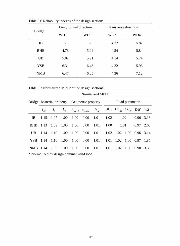
89

Table 3.6 Reliability indexes of the design sections

Bridge Longitudinal direction Transverse direction

WD1 WD3 WD2 WD4

IB - - 4.72 5.82

BHB 4.73 5.04 4.54 5.84

UB 5.82 5.91 4.14 5.74

YSB 6.31 6.43 4.22 5.96

NMB 6.47 6.65 4.36 7.12

Table 3.7 Normalized MPFP of the design sections

Bridge

Normalized MPFP

Material property Geometric property Load parameter

fck fy Es As,avg ηs,avg Agt DCP DCG DCC DW WS*

IB 1.15 1.07 1.00 1.00 0.00 1.01 1.02 1.02 0.96 3.13

BHB 1.13 1.09 1.00 1.00 0.00 1.01 1.00 1.01 0.97 2.63

UB 1.14 1.10 1.00 1.00 0.00 1.01 1.02 1.02 1.00 0.96 3.14

YSB 1.14 1.10 1.00 1.00 0.00 1.01 1.01 1.02 1.00 0.97 1.85

NMB 1.14 1.06 1.00 1.00 0.00 1.01 1.01 1.02 1.00 0.98 3.33 * Normalized by design nominal wind load

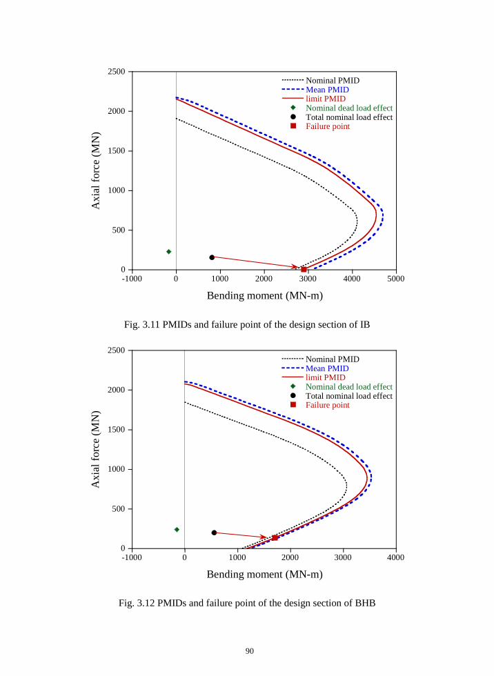
90

Fig. 3.11 PMIDs and failure point of the design section of IB

Fig. 3.12 PMIDs and failure point of the design section of BHB

0

500

1000

1500

2000

2500

-1000 0 1000 2000 3000 4000 5000

Nominal PMIDMean PMIDlimit PMIDNominal dead load effectTotal nominal load effectFailure point

Axi

al fo

rce

(MN

)

Bending moment (MN-m)

0

500

1000

1500

2000

2500

-1000 0 1000 2000 3000 4000


Axi

al fo

rce

(MN

)


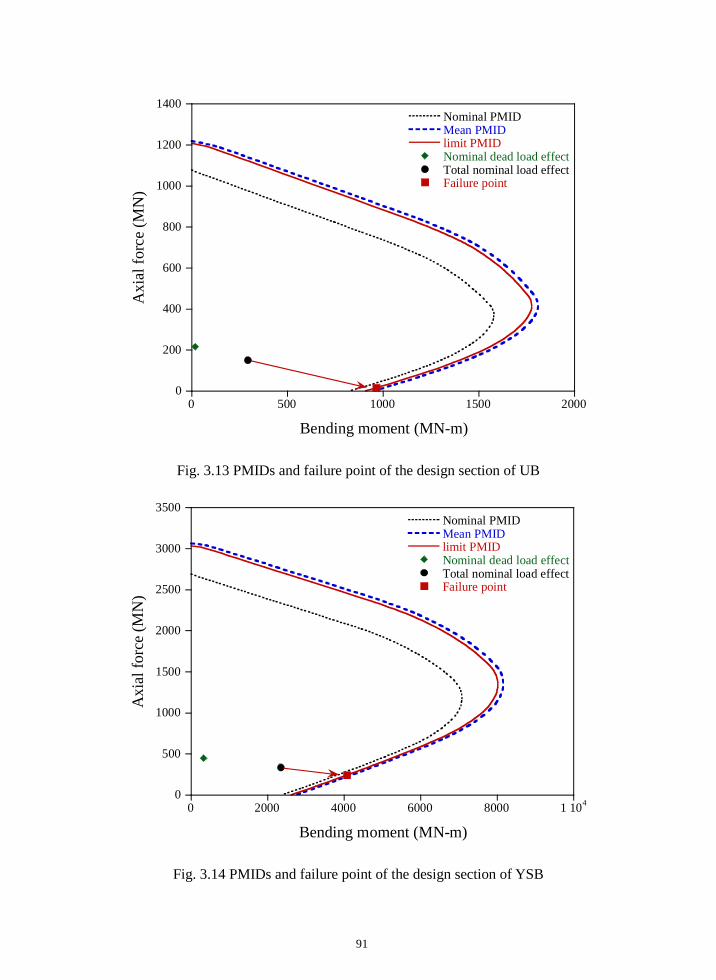
91

Fig. 3.13 PMIDs and failure point of the design section of UB

Fig. 3.14 PMIDs and failure point of the design section of YSB

0

200

400

600

800

1000

1200

1400

0 500 1000 1500 2000


Axi

al fo

rce

(MN

)


0

500

1000

1500

2000

2500

3000

3500

0 2000 4000 6000 8000 1 104


Axi

al fo

rce

(MN

)


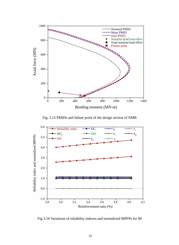
92

Fig. 3.15 PMIDs and failure point of the design section of NMB

Fig 3.16 Variations of reliability indexes and normalized MPFPs for IB

0

200

400

600

800

1000

0 200 400 600 800 1000 1200 1400


Axi

al fo

rce

(MN

)


-1.0

0.0

1.0

2.0

3.0

4.0

5.0

6.0

2.8 3.0 3.2 3.4 3.6 3.8 4.0 4.2

Reliailiby indexDCp

WS

DCc

DWfck

fy

Es

ηs

As

Agt

Rel

iabi

lity

inde

x an

d no

rmal

ized

MPF

Ps

Reinforcement ratio (%)

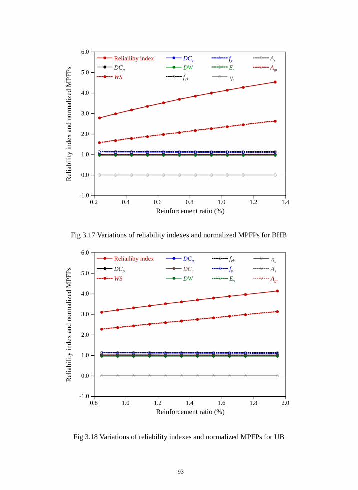
93

Fig 3.17 Variations of reliability indexes and normalized MPFPs for BHB

Fig 3.18 Variations of reliability indexes and normalized MPFPs for UB

-1.0

0.0

1.0

2.0

3.0

4.0

5.0

6.0

0.2 0.4 0.6 0.8 1.0 1.2 1.4

Reliailiby indexDCp

WS

DCc

DWfck

fy

Es

ηs

As

AgtR

elia

bilit

y in

dex

and

norm

aliz

ed M

PFPs


-1.0

0.0

1.0

2.0

3.0

4.0

5.0

6.0

0.8 1.0 1.2 1.4 1.6 1.8 2.0

Reliailiby indexDCp

WS

DCg

DCc

DW

fck

fy

Es

ηs

As

Agt

Rel

iabi

lity

inde

x an

d no

rmal

ized

MPF

Ps


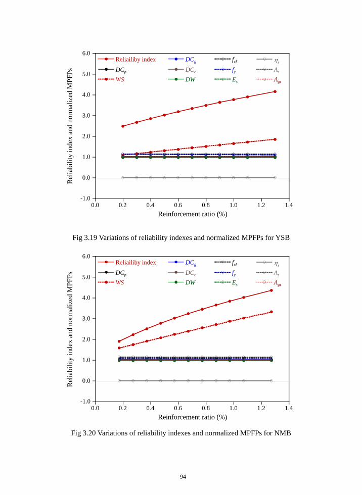
94

Fig 3.19 Variations of reliability indexes and normalized MPFPs for YSB

Fig 3.20 Variations of reliability indexes and normalized MPFPs for NMB

-1.0

0.0

1.0

2.0

3.0

4.0

5.0

6.0

0.0 0.2 0.4 0.6 0.8 1.0 1.2 1.4

Reliailiby indexDCp

WS

DCg

DCc

DW

fck

fy

Es

ηs

As

Agt

Rel

iabi

lity

inde

x an

d no

rmal

ized

MPF

Ps


-1.0

0.0

1.0

2.0

3.0

4.0

5.0

6.0

0.0 0.2 0.4 0.6 0.8 1.0 1.2 1.4

Reliailiby indexDCp

WS

DCg

DCc

DW

fck

fy

Es

ηs

As

Agt

Rel

iabi

lity

inde

x an

d no

rmal

ized

MPF

Ps


95

SECTION 4

CALIBRATION OF WIND LOAD FACTOR

A calibration process for the dead load and wind load factors is presented for the

WGLS, and the proposed load factors are verified for the pylon sections of the five

bridges mentioned in Section 3.3. The load combination under a strong wind is

defined as Strength III Limit State (StrLS-3) in the AASHTO specifications

(AASHTO, 2014), and includes several minor load components such as support

settlement and uniform temperature change. However, the minor load compo-

nents are not generally considered in the calibration process (Bartlett et al., 2003;

Ellingwood et al., 1980; Ellingwood and Tekie, 1999; Nowak, 1999), and thus only

the dead and wind loads are included for calibration in this study. The statistical

uncertainties in the geometric properties have little effect on the results of reliabil-

ity analysis as shown in Section 3.3, and thus the geometric properties are not con-

sidered as random variables in this section. In forthcoming derivations, the bias

factor and nominal value of random variable X are denoted as Xλ and NX , re-

spectively.

The author and coworkers presented evaluations of the wind load factors for

WGLS in reliability-based design codes (Kim et al., 2017). In Section 4.1, an

analytical expression for the base wind load factor is derived, and a design equation

of the WGLS is proposed based on the results of the reliability assessment. In

Section 4.2, the proposed wind load factor is adjusted for the AASHTO specifica-

tions in which the dead load factors and design equation specified in the specifica-

tions are adopted. In Section 4.3, the adjustment procedure is applied to KHBDC

(LSD)-CB and KHBDC (LSD). The wind load factor for KHBDC (LSD)-CB is

96

expressed as a function of the COV of wind velocity, and the basic wind velocities

for KHBDC (LSD) are suggested to secure a uniform reliability level. Section 4.4

shows the validity of the wind load factors is demonstrated for various sizes of a

cross-section.

4.1 Base Load Factors and Design Equations

The discussion on the failure states of the pylons presented at the end of the section

3.3 reveals a motivating fact to determine the load factors for StrLS-3. The pylon

sections reach the limit state due to a dominant increase in the wind load, while the

other random variables remain near their mean values. Since this fact is inferred

purely from the statistical characteristics of the random variables considered in

StrLS-3, it is presumed without loss of generality that the MPFPs of all random

variables except the wind load are fixed at their mean values in the WGLS.

The reliability index is interpreted as the distance between the MPFP and the

origin of the standard normal space. Owing to the aforementioned assumption,

the MPFPs of the random variables other than wind load should be positioned at

the origins of the corresponding variable axes in the standard normal space. The

target reliability index for StrLS-3 simply equals the distance between the MPFP of

the wind load and the origin of the standard normal space.

eqWS

eqWSfT

WS)(

)(σ

µ−=β (4.1)

where βT , WSf, (µWS )eq, and (σWS )eq are the target reliability for StrLS-3, the

MPFP of the wind load, the mean, and the SD of the equivalent normal distribution

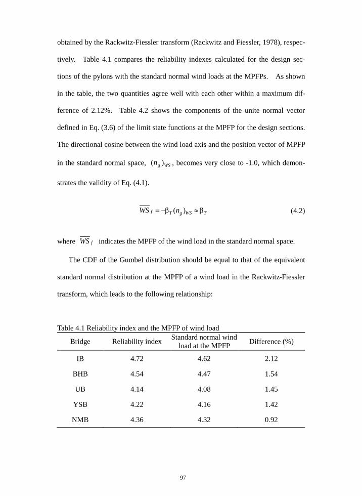
97

obtained by the Rackwitz-Fiessler transform (Rackwitz and Fiessler, 1978), respec-

tively. Table 4.1 compares the reliability indexes calculated for the design sec-

tions of the pylons with the standard normal wind loads at the MPFPs. As shown

in the table, the two quantities agree well with each other within a maximum dif-

ference of 2.12%. Table 4.2 shows the components of the unite normal vector

defined in Eq. (3.6) of the limit state functions at the MPFP for the design sections.

The directional cosine between the wind load axis and the position vector of MPFP

in the standard normal space, WSgn )( , becomes very close to -1.0, which demon-

strates the validity of Eq. (4.1).

TWSgTf nWS β≈β−= )( (4.2)

where fWS indicates the MPFP of the wind load in the standard normal space.

The CDF of the Gumbel distribution should be equal to that of the equivalent

standard normal distribution at the MPFP of a wind load in the Rackwitz-Fiessler

transform, which leads to the following relationship:

Table 4.1 Reliability index and the MPFP of wind load

Bridge Reliability index Standard normal wind load at the MPFP Difference (%)

IB 4.72 4.62 2.12

BHB 4.54 4.47 1.54

UB 4.14 4.08 1.45

YSB 4.22 4.16 1.42

NMB 4.36 4.32 0.92

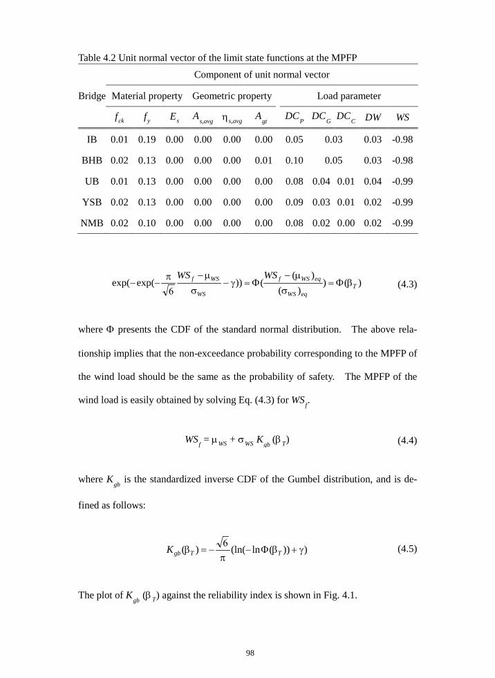
98

Table 4.2 Unit normal vector of the limit state functions at the MPFP

Bridge

Component of unit normal vector


fck fy Es As,avg ηs,avg Agt DCP DCG DCC DW WS

IB 0.01 0.19 0.00 0.00 0.00 0.00 0.05 0.03 0.03 -0.98

BHB 0.02 0.13 0.00 0.00 0.00 0.01 0.10 0.05 0.03 -0.98

UB 0.01 0.13 0.00 0.00 0.00 0.00 0.08 0.04 0.01 0.04 -0.99

YSB 0.02 0.13 0.00 0.00 0.00 0.00 0.09 0.03 0.01 0.02 -0.99

NMB 0.02 0.10 0.00 0.00 0.00 0.00 0.08 0.02 0.00 0.02 -0.99

)())(

)(())exp(exp( T

eqWS

eqWSf

WS

WSf WSWSβΦ=

σ

µ−Φ=γ−

σ

µ−

6π

−− (4.3)

where Φ presents the CDF of the standard normal distribution. The above rela-

tionship implies that the non-exceedance probability corresponding to the MPFP of

the wind load should be the same as the probability of safety. The MPFP of the

wind load is easily obtained by solving Eq. (4.3) for WSf.

WSf = µWS + σWS Kgb (βT) (4.4)

where Kgb is the standardized inverse CDF of the Gumbel distribution, and is de-

fined as follows:

)))(ln(ln()( γ+βΦ−π6

−=β TTgbK (4.5)

The plot of Kgb (βT) against the reliability index is shown in Fig. 4.1.

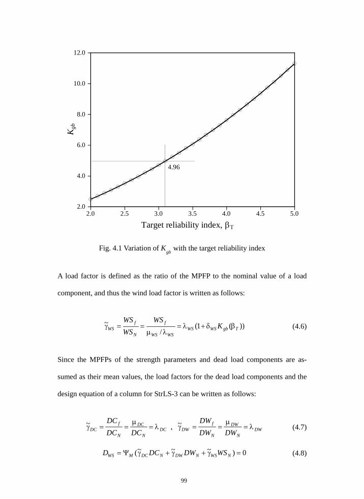
99

Fig. 4.1 Variation of Kgb with the target reliability index

A load factor is defined as the ratio of the MPFP to the nominal value of a load

component, and thus the wind load factor is written as follows:

))(1(/

~TgbWSWS

WSWS

f

N

fWS K

WSWSWS

βδ+λ=λµ

==γ (4.6)

Since the MPFPs of the strength parameters and dead load components are as-

sumed as their mean values, the load factors for the dead load components and the

design equation of a column for StrLS-3 can be written as follows:

DWN

DW

N

fDWDC

N

DC

N

fDC DWDW

DWDCDC

DCλ=

µ==γλ=

µ==γ ~ , ~ (4.7)

0)~~~( =γ+γ+γΨ= NWSNDWNDCMWS WSDWDCD (4.8)

2.0

4.0

6.0

8.0

10.0

12.0

2.0 2.5 3.0 3.5 4.0 4.5 5.0

K gb

Target reliability index, βΤ

4.96

100

In Eqs. (4.6), (4.7), and (4.8), Xγ~ denotes the proposed load factor of load com-

ponent X, and MΨ is the mean PMID of a column. The load factors defined in

Eqs. (4.6) and (4.7) are hereafter referred to as the base wind and dead load factors,

respectively. In Fig. 4.2, the proposed wind load factors based on Eq. (4.6) for

λWS = 1 and δWS = 0.27, 0.30 and 0.33 are illustrated with solid lines. Table 4.3

shows the base wind load factors for the reliability indexes of 2.7, 3.1, and 3.5 for

the three COVs of the wind load.

The validity of the base wind load factor and the design equation defined in Eq.

(4.8) is tested through the following validation analysis. A base wind load factor

corresponding to a specific target reliability index is selected using Eq. (4.6), and

the total factored load effect for the limit state is evaluated for each of the pylons

for the five bridges. The pylon section that exactly satisfies Eq. (4.8) for the total

factored load effect is selected by adjusting the reinforcement ratio while the other

strength parameters are fixed at their mean values. The cross-sectional area of

each reinforcing steel is adjusted while the reinforcement arrangement and the ge-

ometry of the original section are kept fixed. Since the PMID is a nonlinear func-

tion, the bi-section method is utilized to find the required reinforcement ratio for

each pylon section satisfying the design equation. The reliability index of the sec-

tion with the adjusted reinforcement ratio is calculated using the AFOSM defined

in Eq. (3.5) and compared with the reliability index corresponding to the selected

base wind load factor. If the two reliability indexes coincide with each other

within an acceptable error tolerance, the validity of the base load factor and the

design equation is confirmed.

The aforementioned validation analysis is applied to each pylon section for the

nine wind load factors given in Table 4.3 to ensure the generality of the base load

101

factor. The bias factors of the dead load components in Table 3.2 are utilized.

The wind load effects corresponding to λWS = 1 are presented for the longitudinal

and transverse direction WS in Tables 4.4 and 4.5, respectively. The results of

analyses including the adjusted reinforcement ratios, ρAdj, the calculated reliability

indexes, βC and the MPFPs of the random variables are shown in Table 4.6 for

49.2~ =γWS and δWS = 0.30. The base wind load factor of 2.49 corresponds to the

target reliability of 3.1. Table 4.6 shows that the MPFP of all the random varia-

bles except for wind load remain near their mean values as assumed. It should be

noted that the MPFP for the other cases, which are not presented in this work, ex-

hibit similar patterns to those given in Table 4.6. The reliability indexes are cal-

culated for the adjusted reinforcement ratio based on the base wind load factors

given in Table 4.3, and are marked with the centered symbols in Fig. 4.2. The

shapes of the centered symbols indicate the individual bridges, and the blue-,

black- and red- centered symbols correspond to δWS = 0.27, 0.30 and 0.33, respec-

tively. The vertical lines in the plot indicate the specified reliability indexes to

select the wind load factors by Eq. (4.6). As shown in the plot, the proposed base

load factors and design equation yield slightly lower reliability indexes than the

target within an 1.5% error. The small discrepancy between the target and the

calculated reliability indexes is caused by the fact the MPFPs of the strength pa-

rameters, which are calculated to be somewhat lower than the mean values in the

AFOSM, do not exactly satisfy the assumption made in the derivation. The error,

however, is negligibly small from an engineering viewpoint, and the proposed load

factors are believed to be justifiable values that could be adopted in a design code.

The calculated reliability indexes of the five bridges for a base wind load factor are

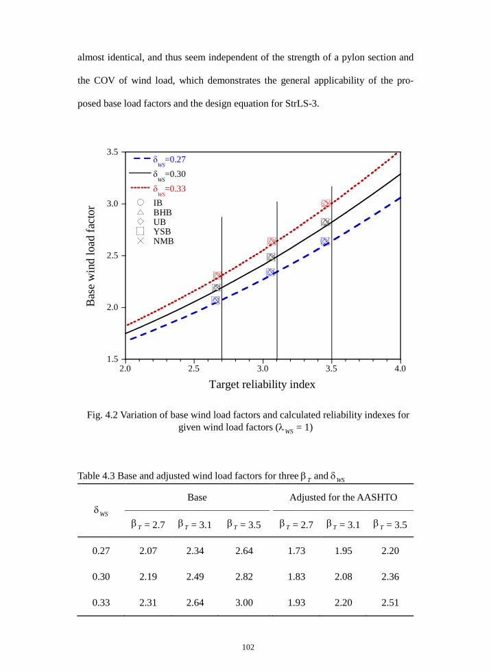
102

almost identical, and thus seem independent of the strength of a pylon section and

the COV of wind load, which demonstrates the general applicability of the pro-

posed base load factors and the design equation for StrLS-3.

Fig. 4.2 Variation of base wind load factors and calculated reliability indexes for given wind load factors (λWS = 1)

Table 4.3 Base and adjusted wind load factors for three βT and δWS

δWS Base Adjusted for the AASHTO

βT = 2.7 βT = 3.1 βT = 3.5 βT = 2.7 βT = 3.1 βT = 3.5

0.27 2.07 2.34 2.64 1.73 1.95 2.20

0.30 2.19 2.49 2.82 1.83 2.08 2.36

0.33 2.31 2.64 3.00 1.93 2.20 2.51

1.5

2.0

2.5

3.0

3.5

2.0 2.5 3.0 3.5 4.0

δWS

=0.27δ

WS=0.30

δWS

=0.33IBBHBUBYSBNMB

Bas

e w

ind

load

fact

or

Target reliability index

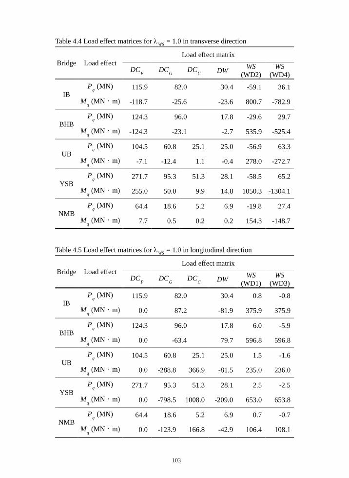
103

Table 4.4 Load effect matrices for λWS = 1.0 in transverse direction


DCP DCG DCC DW WS

(WD2) WS

(WD4)

IB Pq (MN) 115.9 82.0 30.4 -59.1 36.1

Mq (MN·m) -118.7 -25.6 -23.6 800.7 -782.9

BHB Pq (MN) 124.3 96.0 17.8 -29.6 29.7

Mq (MN·m) -124.3 -23.1 -2.7 535.9 -525.4

UB Pq (MN) 104.5 60.8 25.1 25.0 -56.9 63.3

Mq (MN·m) -7.1 -12.4 1.1 -0.4 278.0 -272.7

YSB Pq (MN) 271.7 95.3 51.3 28.1 -58.5 65.2

Mq (MN·m) 255.0 50.0 9.9 14.8 1050.3 -1304.1

NMB Pq (MN) 64.4 18.6 5.2 6.9 -19.8 27.4

Mq (MN·m) 7.7 0.5 0.2 0.2 154.3 -148.7

Table 4.5 Load effect matrices for λWS = 1.0 in longitudinal direction


DCP DCG DCC DW WS

(WD1) WS

(WD3)

IB Pq (MN) 115.9 82.0 30.4 0.8 -0.8

Mq (MN·m) 0.0 87.2 -81.9 375.9 375.9

BHB Pq (MN) 124.3 96.0 17.8 6.0 -5.9

Mq (MN·m) 0.0 -63.4 79.7 596.8 596.8

UB Pq (MN) 104.5 60.8 25.1 25.0 1.5 -1.6

Mq (MN·m) 0.0 -288.8 366.9 -81.5 235.0 236.0

YSB Pq (MN) 271.7 95.3 51.3 28.1 2.5 -2.5

Mq (MN·m) 0.0 -798.5 1008.0 -209.0 653.0 653.8

NMB Pq (MN) 64.4 18.6 5.2 6.9 0.7 -0.7

Mq (MN·m) 0.0 -123.9 166.8 -42.9 106.4 108.1

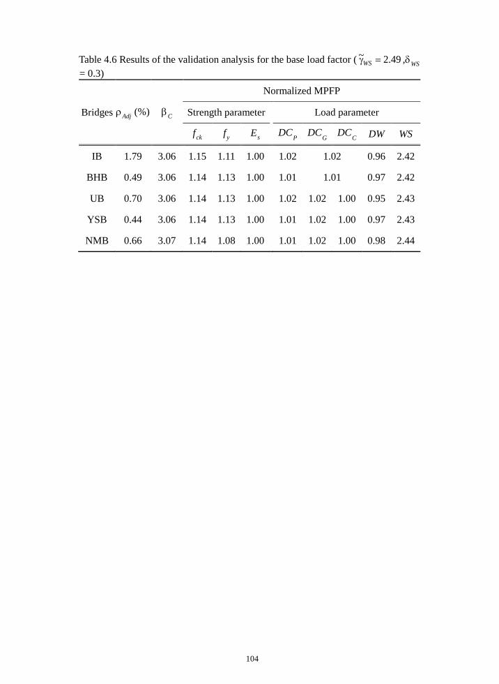
104

Table 4.6 Results of the validation analysis for the base load factor ( 49.2~ =γWS ,δWS

= 0.3)

Bridges ρAdj (%) βC

Normalized MPFP

Strength parameter Load parameter

fck fy Es DCP DCG DCC DW WS

IB 1.79 3.06 1.15 1.11 1.00 1.02 1.02 0.96 2.42

BHB 0.49 3.06 1.14 1.13 1.00 1.01 1.01 0.97 2.42

UB 0.70 3.06 1.14 1.13 1.00 1.02 1.02 1.00 0.95 2.43

YSB 0.44 3.06 1.14 1.13 1.00 1.01 1.02 1.00 0.97 2.43

NMB 0.66 3.07 1.14 1.08 1.00 1.01 1.02 1.00 0.98 2.44

105

4.2 Adjustment for AASHTO Specifications

The AASHTO specifications (AASHTO, 2014) adopt the same dead load factors

for StrLS-3 as those of Strength I Limit State. The design PMID is obtained by

multiplying a resistance factor to the nominal PMID. The resistance factor of a

non-presetressed column, φR, in the AASHTO specifications is given as follows:

9.0)(15.075.075.0 ≤ε−ε

ε−ε+=φ≤

cltl

cltR (4.9)

where εt, εcl, and εtl denote the net tensile strain in the extreme tension steel at

nominal resistance, the compression-controlled strain limit in the extreme tension

steel, and the tension-controlled strain limit in the extreme tension steel, respective-

ly. The specified values of εcl and εtl are 0.002 for Grade 60 reinforcements and

0.005 for reinforcing steels with a minimum yield strength less than 517MPa, re-

spectively.

The design equation for StrLS-3 is written in the AASHTO specifications as

follows:

DWS = ΨD (γDC DC + γDW DW + γWS WS) = 0 (4.10)

where γX is the load factor for load component X given in the AASHTO specifica-

tions, and ΨD is the design PMID. In case Eq. (4.10) is adopted as the design

equation, the base wind load factor in Eq. (4.6) should be adjusted to accommodate

the differences in the dead load factors and design equation. The adjustment is

problem-dependent because the ratio of the wind load effect to dead load effect in a

pylon section varies with bridges, and the strength of an RC column is not defined

106

by a single scalar value but by a 2-dimensional PMID. It is rather difficult to ad-

just the wind load factor in a deductive way for the AASHTO specifications. To

circumvent the problem-dependency of the adjustment, this work uses a curve-

fitting approach. An adjustment factor, αWS, is introduced in Eq. (4.6) to find the

wind load factor satisfying the AASHTO specifications.

γWS = αWS λWS (1+ δWS Kgb(βT)) (4.11)

To determine the adjustment factor in Eq. (4.11), the wind load factors yielding the

specified target reliability indexes are calculated with the design equation of Eq.

(4.10). The reinforcement ratio of each pylon section that results in a specified

target reliability index is estimated using the bi-section method operating on the

reliability index calculated by the AFOSM in Eq. (3.5). Once the desired rein-

forcement ratio is determined for a pylon section, the design PIMD in Eq. (4.10) is

formed according to the AASHTO specifications. As all nominal-load effects and

dead load factors are known, the wind load factor that satisfies the design equation

given in Eq. (4.10) is readily evaluated by finding the intersection point between

the line representing the total factored-load effect and the design PMID as illustrat-

ed in Fig. 4.3 for the YSB. To simplify this calculation, the design PMID segment

between two adjacent sampling points is assumed to be a straight line. It is

worthwhile to mention the difference between the previous validation analysis and

the current adjustment procedure. In the former, the reliability index is calculated

for a pylon section determined by the design equation of Eq. (4.8) and a given wind

load factor, while the later determines the wind load factor that would satisfy Eq.

(4.10) and a given reliability index for a pylon section.

The results of the adjustment procedure including the adjusted reinforcement

107

ratios, the calculated wind load factor, CWS )(γ , and the MPFPs of the random var-

iables are shown in Table 4.7 for βT = 3.1 and δWS = 0.3. The wind load factors

that satisfy the AASHTO specifications for the three reliability indexes and COVs

are illustrated in Fig. 4.4 with centered symbols for the five pylon sections. The

notation for the centered symbols in Fig. 4.4 is the same as that used in Fig. 4.2.

The vertical lines in the plot indicate the target reliability indexes used to find the

reinforcement ratios of the pylon sections that satisfy the AASHTO specifications.

The best-fit lines for the wind load factors marked with the centered symbols in Fig.

4.4 are drawn by selecting the adjustment factor as 0.835. The wind load factors

calculated with the adjustment factor are plotted with solid lines in Fig. 4.4, which

shows excellent agreement between the wind load factors predicted by Eq. (4.11)

and those calculated for the five pylons in the adjustment procedure. The adjusted

wind load factors evaluated by Eq. (4.11) are summarized in Table 4.3 for the three

COVs of the wind load and the target reliability indexes.

The reinforcement ratios of the pylon sections in Table 4.6 are smaller than

those in Table 4.7. This is because the reinforcement ratios given in Table 4.6

yield slightly lower reliability indexes than the target as explained earlier, while

those given in Table 4.7 is adjusted to exactly satisfy the target reliability indexes.

The MPFPs of all random variables other than the wind load in Tables 4.6 and 4.7

are identical. The MPFP of the wind load in Table 4.7 are slightly larger than

those in Table 4.6 due to the differences in the reinforcement ratio. These facts

imply that the design equations in Eqs. (4.8) and (4.10) along with the correspond-

ing load factors require the same strength of a column.

As pointed out in NCHRP Report 489 by Ghosn et al. (2003), the current

AASHTO specifications provide a reliability index near 3.0 for the wind load. In

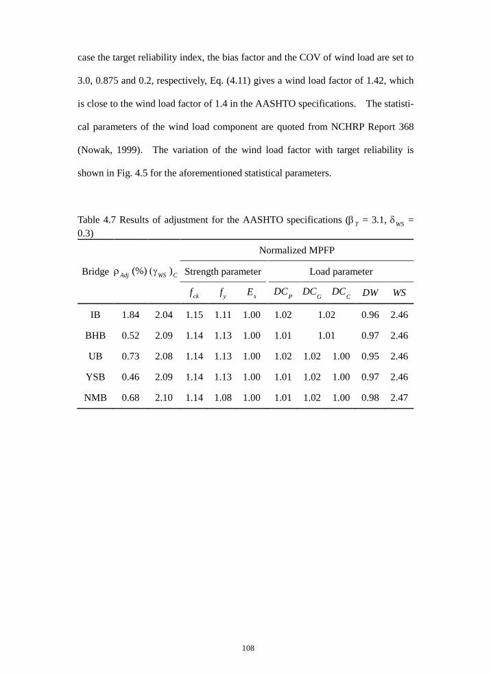
108

case the target reliability index, the bias factor and the COV of wind load are set to

3.0, 0.875 and 0.2, respectively, Eq. (4.11) gives a wind load factor of 1.42, which

is close to the wind load factor of 1.4 in the AASHTO specifications. The statisti-

cal parameters of the wind load component are quoted from NCHRP Report 368

(Nowak, 1999). The variation of the wind load factor with target reliability is

shown in Fig. 4.5 for the aforementioned statistical parameters.

Table 4.7 Results of adjustment for the AASHTO specifications (βT = 3.1, δWS = 0.3)

Bridge ρAdj (%) (γWS )C

Normalized MPFP



IB 1.84 2.04 1.15 1.11 1.00 1.02 1.02 0.96 2.46

BHB 0.52 2.09 1.14 1.13 1.00 1.01 1.01 0.97 2.46

UB 0.73 2.08 1.14 1.13 1.00 1.02 1.02 1.00 0.95 2.46

YSB 0.46 2.09 1.14 1.13 1.00 1.01 1.02 1.00 0.97 2.46

NMB 0.68 2.10 1.14 1.08 1.00 1.01 1.02 1.00 0.98 2.47

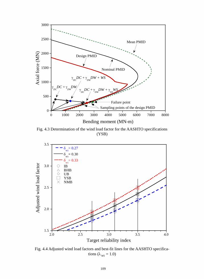
109

Fig. 4.3 Determination of the wind load factor for the AASHTO specifications (YSB)

Fig. 4.4 Adjusted wind load factors and best-fit lines for the AASHTO specifica-tions (λWS = 1.0)

0

500

1000

1500

2000

2500

3000

0 1000 2000 3000 4000 5000 6000 7000 8000

Axi

al fo

rce

(MN

)


γDC

DC + γDW

DW

γDC

DC + γDW

DW + WS

γDC

DC + γDW

DW + γWS

WS

Design PMID

Nominal PMID

Sampling points of the design PMID

Mean PMID

Failure point

1.5

2.0

2.5

3.0

3.5

2.0 2.5 3.0 3.5 4.0

δWS

= 0.27δ

WS= 0.30

δWS

= 0.33IBBHBUBYSBNMB

Adj

uste

d w

ind

load

fact

or


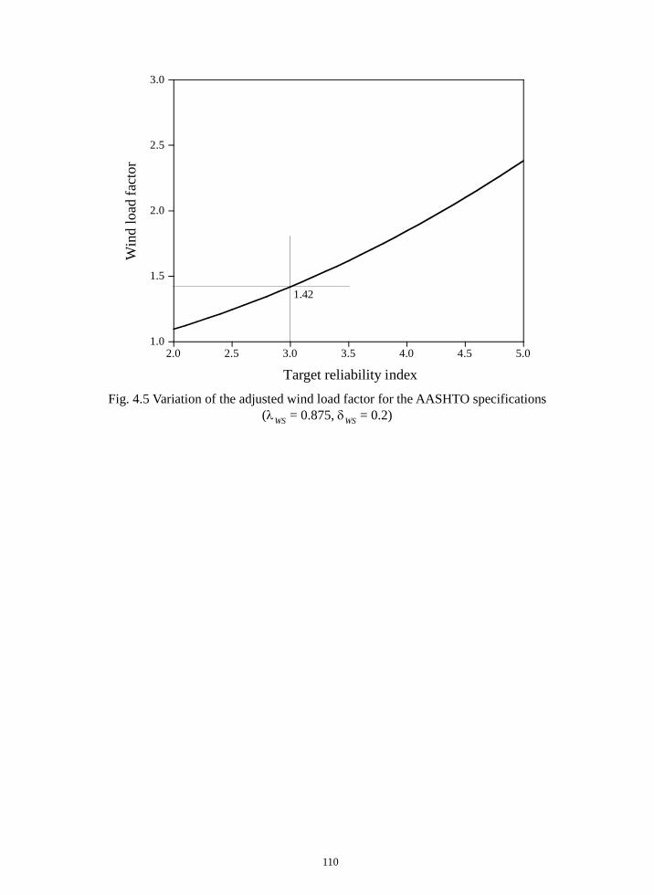
110

Fig. 4.5 Variation of the adjusted wind load factor for the AASHTO specifications

(λWS = 0.875, δWS = 0.2)

1.0

1.5

2.0

2.5

3.0

2.0 2.5 3.0 3.5 4.0 4.5 5.0

Win

d lo

ad fa

ctor


1.42

111

4.3 Adjustment for KHBDC (LSD) and KHBDC (LSD)-CB

Prior to performing the adjustment of the base wind load factor for KHBDC (LSD)

(KMOLIT, 2016a) and KHBDC (LSD)-CB (KMOLIT, 2016b), the validation anal-

ysis in Section 4.1 is conducted using the stress-strain relationships of concrete and

reinforcing steel specified in KHBDC (LSD). The results of the validation analy-

sis for KHBDC (LSD) are exactly the same as Table 4.6 and Fig. 4.2. The differ-

ence in the stress-strain relation, which depends on the design provisions, has little

effect on the reliability analysis and the evaluation of wind load factors. The de-

tails of the comparison of the stress-strain relations are presented in the APPEN-

DIX A.

In KHBDC (LSD), the design strength of RC components (i.e., design PMID)

is estimated by introducing partial safety factors for materials to underestimate the

compressive strength of concrete and the yield strength of reinforcing steels. For

ultimate limit state load combination III (UltLS-3), the partial safety factors of

concrete and reinforcing steels are suggested as φc = 0.65 and φs = 0.9, respectively.

In this section, the design PMID for KHBDC (LSD) and KHBDC (LSD)-CB is

obtained based on the stress-strain relation and the partial safety factors specified in

the APPENDIX A

4.3.1 Adjusted wind load factors for KHBDC (LSD)-CB

KHBDC (LSD)-CB (KMOLIT, 2016b) specifies different load factors for each

dead load due to the self-weight of structural components as shown in Table 4.8.

The stress-strain relations and the partial safety factor of KHBDC (LSD)-CB are

identical to those of KHBDC (LSD). The results of the adjustment for KHBDC

112

(LSD)-CB are summarized in Table 4.9, and presented with centered symbols in

Fig. 4.6. The best-fit line of the wind load factors is drawn with αWS = 0.80 in the

figure.

γWS = 0.80 λWS (1+ δWS Kgb(βT)) (4.12)

The nominal, limit and design PMIDs and the factored load effects are presented in

Fig. 4.7 for the YSB as the representative case for the five bridges. The factored-

dead load effects and total factored load effects are drawn with black and red cir-

cles, respectively. The adjusted wind load factors for KHBDC (LSD)-CB are

summarized in Table 4.10.

The nominal wind load for the UltLS-3 in KHBDC (LSD)-CB is defined as the

basic wind velocity of which the recurrence period is equal to the design life of a

structure. The basic wind velocity for KHBDC (LSD)-CB is calculated by Eq.

(2.14) using the statistical parameters of the wind velocity estimated based on the

measured wind data at the bridge site. The bias factor and COV of the wind

pressure corresponding to the basic wind velocity are calculated by Eqs. (2.20) and

(2.22), respectively, those are required to evaluate the wind load factor as shown in

Eq. (4.12). The wind load factor for KHBDC (LSD)-CB is expressed as a func-

tion of 10Vδ by substituting Eq. (2.20) and Eq. (2.22) into Eq. (4.12).

)()078.2571.1060.0(088.1778.0

))()910.1077.0(1)(360.1973.0(08.02

101010

1010

TgbVVV

TgbVVWS

K

K

βδ+δ++δ+=

βδ++δ+=γ (4.13)

In Fig. 4.8, the adjusted wind load factors based on Eq. (4.13) for 10Vδ = 0.10, 0.11,

0.12, and 0.13 are illustrated with solid lines. The range of the COV of wind ve-

113

locity is selected based on the measured wind data in Korea as shown in Table 2.8.

In case target reliability index is set to 3.1, Eq. (4.13) gives the wind load factors of

2.07, 2.18, 2.29, and 2.40 for 10Vδ = 0.10, 0.11, 0.12, and 0.13, respectively. The

wind load factor increases rapidly with respect to the target reliability index for

large COV of the wind velocity in Fig. 4.8. The wind load factor in the current

version of KHBDC (LSD)-CB is proposed as 1.7, which implies that the current

wind load factor secures the reliability level from 2.0 to 2.4 for the given range of

the COV of wind velocity.

For the sake of simplicity, the coefficient of )( TgbK β in Eq. (4.3) is approxi-

mated as a linear function of 10Vδ as shown in Fig. 4.9.

101010204.0078.2571.1060.0 2

VVV δ+≈δ+δ+ (4.14)

The standardized inverse CDF of the Gumbel distribution, )( TgbK β , is approxi-

mated based on the best-fit lines in the range of 0.50.2 ≤β≤ T as shown in Fig.

4.10.

))(36.038.028.0()))(ln(ln(6)( 2TTTTgbK β+β+≈γ+βΦ−

π−=β (4.15)

The wind load factor in Eq. (4.13) is presented by substituting the Eq. (4.14) and

Eq. (4.15) into the equation.

))(36.038.028.0)(204.0(09.179.0

)()204.0(09.179.02

1010

1010

TTVV

TgbVVWS K

β+β+δ++δ+≈

βδ++δ+≈γ (4.16)

For 1.3=βT , the approximated wind load factor for KHBDC (LSD)-CB is simply

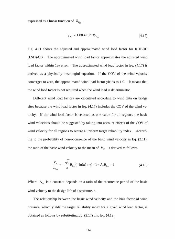
114

expressed as a linear function of 10Vδ .

1093.1000.1 VWS δ+≈γ (4.17)

Fig. 4.11 shows the adjusted and approximated wind load factor for KHBDC

(LSD)-CB. The approximated wind load factor approximates the adjusted wind

load factor within 1% error. The approximated wind load factor in Eq. (4.17) is

derived as a physically meaningful equation. If the COV of the wind velocity

converges to zero, the approximated wind load factor yields to 1.0. It means that

the wind load factor is not required when the wind load is deterministic.

Different wind load factors are calculated according to wind data on bridge

sites because the wind load factor in Eq. (4.17) includes the COV of the wind ve-

locity. If the wind load factor is selected as one value for all regions, the basic

wind velocities should be suggested by taking into account effects of the COV of

wind velocity for all regions to secure a uniform target reliability index. Accord-

ing to the probability of non-occurrence of the basic wind velocity in Eq. (2.11),

the ratio of the basic wind velocity to the mean of 10V is derived as follows.

11))ln((61010

10

+δΛ=+γ+−δπ

−=µ VnV

V

B nV (4.18)

Where nΛ is a constant depends on a ratio of the recurrence period of the basic

wind velocity to the design life of a structure, n.

The relationship between the basic wind velocity and the bias factor of wind

pressure, which yields the target reliability index for a given wind load factor, is

obtained as follows by substituting Eq. (2.17) into Eq. (4.12).

115

2ˆ

2ˆ )()(

))(1(80.010

B

VqVq

TgbWS

WSWS VK WSBWS

µµ=λµ=

βδ+γ

=λ (4.19)

Based on Eq. (4.19), the ratio of the basic wind velocity to the mean of V10 for a

wind load factor of 1.0 is expressed in terms of statistical parameters of wind pres-

sure.

WSWS qTgbqV

B KVˆˆ ))(1(80.0

10

µβδ+=µ

(4.20)

In Eq. (4.20), the COV of the normalized wind pressure is used instead of the COV

of wind pressure based on Eq. (2.21). The standardized inverse CDF of the

Gumbel distribution is derived from the condition that Eq. (4.18) is always equal to

Eq. (4.20).

)1)1(25.1(1)1)(25.1(1 2

ˆˆ

2

ˆ10

10

−+δΛµδ

=−µµδ

= VnqqV

B

qWSgb

WSWSWS

VK (4.21)

The mean and COV of the normalized wind pressure presented in Eqs. (2.16) and

(2.22) are utilized to express Eq. (4.21) as a function of the COV of wind velocity.

)1)1(239.0986.0

25.1(910.1077.0

1),( 210

1010

10−+δΛ

δ+δ+=δΛ Vn

VVVnRK (4.22)

Where ),(10VnRK δΛ indicates the standardized inverse CDF of the Gumbel dis-

tribution presented by a function of the COV of wind velocity and the recurrence

period of the basic wind velocity. The variations of the standardized inverse CDF

of the Gumbel distribution are illustrated in Fig. 4.12 for the COV of wind velocity

in conjunction with a wind load factor of 1.0. The K R corresponding to the COV

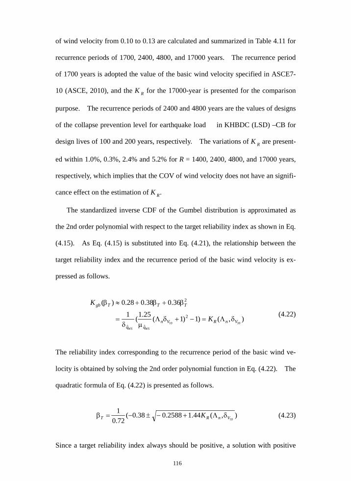
116

of wind velocity from 0.10 to 0.13 are calculated and summarized in Table 4.11 for

recurrence periods of 1700, 2400, 4800, and 17000 years. The recurrence period

of 1700 years is adopted the value of the basic wind velocity specified in ASCE7-

10 (ASCE, 2010), and the K R for the 17000-year is presented for the comparison

purpose. The recurrence periods of 2400 and 4800 years are the values of designs

of the collapse prevention level for earthquake load in KHBDC (LSD) –CB for

design lives of 100 and 200 years, respectively. The variations of K R are present-

ed within 1.0%, 0.3%, 2.4% and 5.2% for R = 1400, 2400, 4800, and 17000 years,

respectively, which implies that the COV of wind velocity does not have an signifi-

cance effect on the estimation of K R.

The standardized inverse CDF of the Gumbel distribution is approximated as

the 2nd order polynomial with respect to the target reliability index as shown in Eq.

(4.15). As Eq. (4.15) is substituted into Eq. (4.21), the relationship between the

target reliability index and the recurrence period of the basic wind velocity is ex-

pressed as follows.

),()1)1(25.1(1

36.038.028.0)(

1010

2

ˆˆ

2

VnRVnqq

TTTgb

K

K

WSWS

δΛ=−+δΛµδ

=

β+β+≈β (4.22)

The reliability index corresponding to the recurrence period of the basic wind ve-

locity is obtained by solving the 2nd order polynomial function in Eq. (4.22). The

quadratic formula of Eq. (4.22) is presented as follows.

),(44.12588.038.0(72.01

10VnRT K δΛ+−±−=β (4.23)

Since a target reliability index always should be positive, a solution with positive

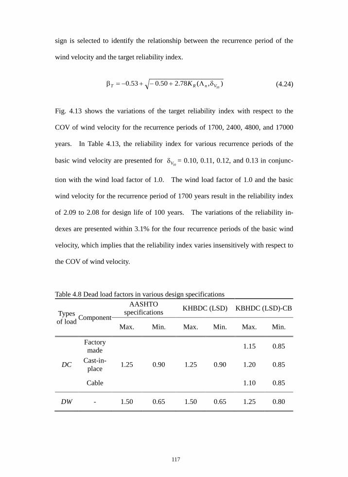
117

sign is selected to identify the relationship between the recurrence period of the

wind velocity and the target reliability index.

),(78.250.053.0

10VnRT K δΛ+−+−=β (4.24)

Fig. 4.13 shows the variations of the target reliability index with respect to the

COV of wind velocity for the recurrence periods of 1700, 2400, 4800, and 17000

years. In Table 4.13, the reliability index for various recurrence periods of the

basic wind velocity are presented for 10Vδ = 0.10, 0.11, 0.12, and 0.13 in conjunc-

tion with the wind load factor of 1.0. The wind load factor of 1.0 and the basic

wind velocity for the recurrence period of 1700 years result in the reliability index

of 2.09 to 2.08 for design life of 100 years. The variations of the reliability in-

dexes are presented within 3.1% for the four recurrence periods of the basic wind

velocity, which implies that the reliability index varies insensitively with respect to

the COV of wind velocity.

Table 4.8 Dead load factors in various design specifications

Types of load Component

AASHTO specifications KHBDC (LSD) KBHDC (LSD)-CB

Max. Min. Max. Min. Max. Min.

DC

Factory made

1.25 0.90 1.25 0.90

1.15 0.85

Cast-in-place 1.20 0.85

Cable 1.10 0.85

DW - 1.50 0.65 1.50 0.65 1.25 0.80

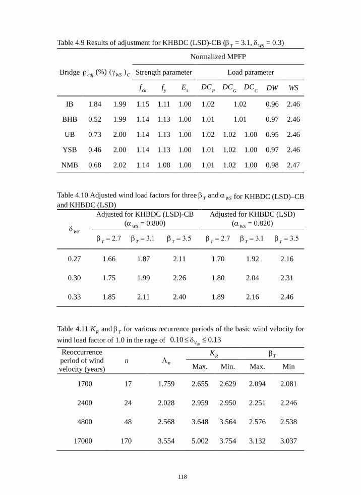
118

Table 4.9 Results of adjustment for KHBDC (LSD)-CB (βT = 3.1, δWS = 0.3)

Bridge ρadj (%) (γWS )C

Normalized MPFP



IB 1.84 1.99 1.15 1.11 1.00 1.02 1.02 0.96 2.46

BHB 0.52 1.99 1.14 1.13 1.00 1.01 1.01 0.97 2.46

UB 0.73 2.00 1.14 1.13 1.00 1.02 1.02 1.00 0.95 2.46

YSB 0.46 2.00 1.14 1.13 1.00 1.01 1.02 1.00 0.97 2.46

NMB 0.68 2.02 1.14 1.08 1.00 1.01 1.02 1.00 0.98 2.47

Table 4.10 Adjusted wind load factors for three βT and αWS for KHBDC (LSD)–CB and KHBDC (LSD)

δWS

Adjusted for KHBDC (LSD)-CB (αWS = 0.800)

Adjusted for KHBDC (LSD) (αWS = 0.820)

βT = 2.7 βT = 3.1 βT = 3.5 βT = 2.7 βT = 3.1 βT = 3.5

0.27 1.66 1.87 2.11 1.70 1.92 2.16

0.30 1.75 1.99 2.26 1.80 2.04 2.31

0.33 1.85 2.11 2.40 1.89 2.16 2.46

Table 4.11 KR and βT for various recurrence periods of the basic wind velocity for wind load factor of 1.0 in the rage of 13.010.0

10≤δ≤ V

Reoccurrence period of wind velocity (years)

n nΛ KR Tβ

Max. Min. Max. Min

1700 17 1.759 2.655 2.629 2.094 2.081

2400 24 2.028 2.959 2.950 2.251 2.246

4800 48 2.568 3.648 3.564 2.576 2.538

17000 170 3.554 5.002 3.754 3.132 3.037

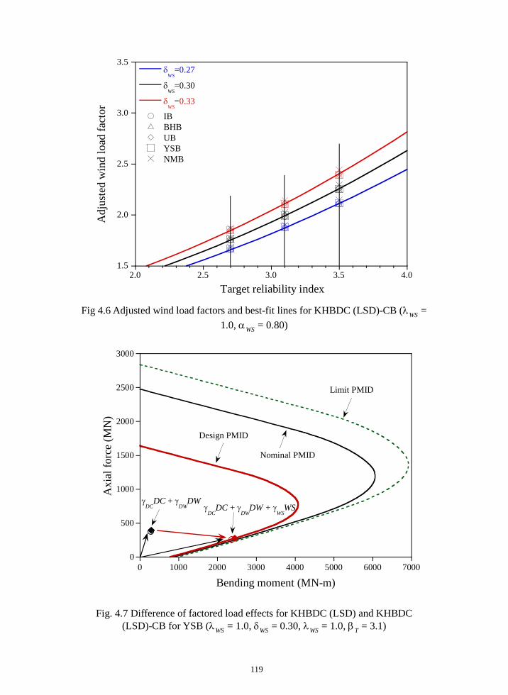
119

Fig 4.6 Adjusted wind load factors and best-fit lines for KHBDC (LSD)-CB (λWS = 1.0, αWS = 0.80)

Fig. 4.7 Difference of factored load effects for KHBDC (LSD) and KHBDC

(LSD)-CB for YSB (λWS = 1.0, δWS = 0.30, λWS = 1.0, βT = 3.1)

1.5

2.0

2.5

3.0

3.5

2.0 2.5 3.0 3.5 4.0

δWS

=0.27

δWS

=0.30

δWS

=0.33

IBBHBUBYSBNMB

Adj

uste

d w

ind

load

fact

or


0

500

1000

1500

2000

2500

3000

0 1000 2000 3000 4000 5000 6000 7000

Axi

al fo

rce

(MN

)


γDC

DC + γDW

DWγ

DCDC + γ

DWDW + γ

WSWS

Design PMID

Nominal PMID

Limit PMID

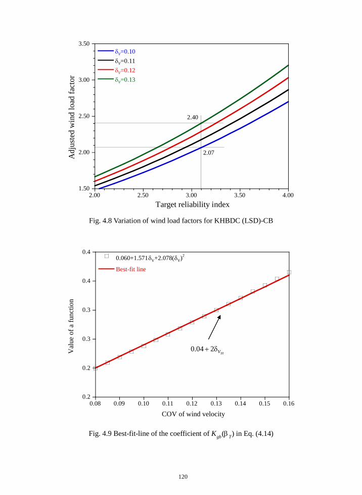
120

Fig. 4.8 Variation of wind load factors for KHBDC (LSD)-CB

Fig. 4.9 Best-fit-line of the coefficient of Kgb(βT) in Eq. (4.14)

1.50

2.00

2.50

3.00

3.50

2.00 2.50 3.00 3.50 4.00

δV=0.10δV=0.11δV=0.12δV=0.13

Adj

uste

d w

ind

load

fact

or


2.40

2.07

0.2

0.2

0.3

0.3

0.4

0.4

0.08 0.09 0.10 0.11 0.12 0.13 0.14 0.15 0.16

0.060+1.571δV+2.078(δV)2

Best-fit line

Val

ue o

f a fu

nctio

n


10204.0 Vδ+

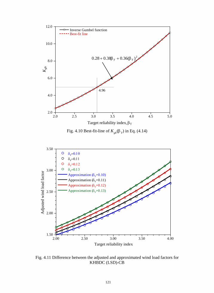
121

Fig. 4.10 Best-fit-line of Kgb(βT) in Eq. (4.14)

Fig. 4.11 Difference between the adjusted and approximated wind load factors for

KHBDC (LSD)-CB

2.0

4.0

6.0

8.0

10.0

12.0

2.0 2.5 3.0 3.5 4.0 4.5 5.0

Inverse Gumbel functionBest-fit line

K gb

Target reliability index, βΤ

4.96

2)(36.038.028.0 TT β+β+

1.50

2.00

2.50

3.00

3.50

2.00 2.50 3.00 3.50 4.00

δV=0.10δV=0.11δV=0.12δV=0.13Approximation (δV=0.10)Approximation (δV=0.11)Approximation (δV=0.12)Approximation (δV=0.13)

Adj

uste

d w

ind

load

fact

or


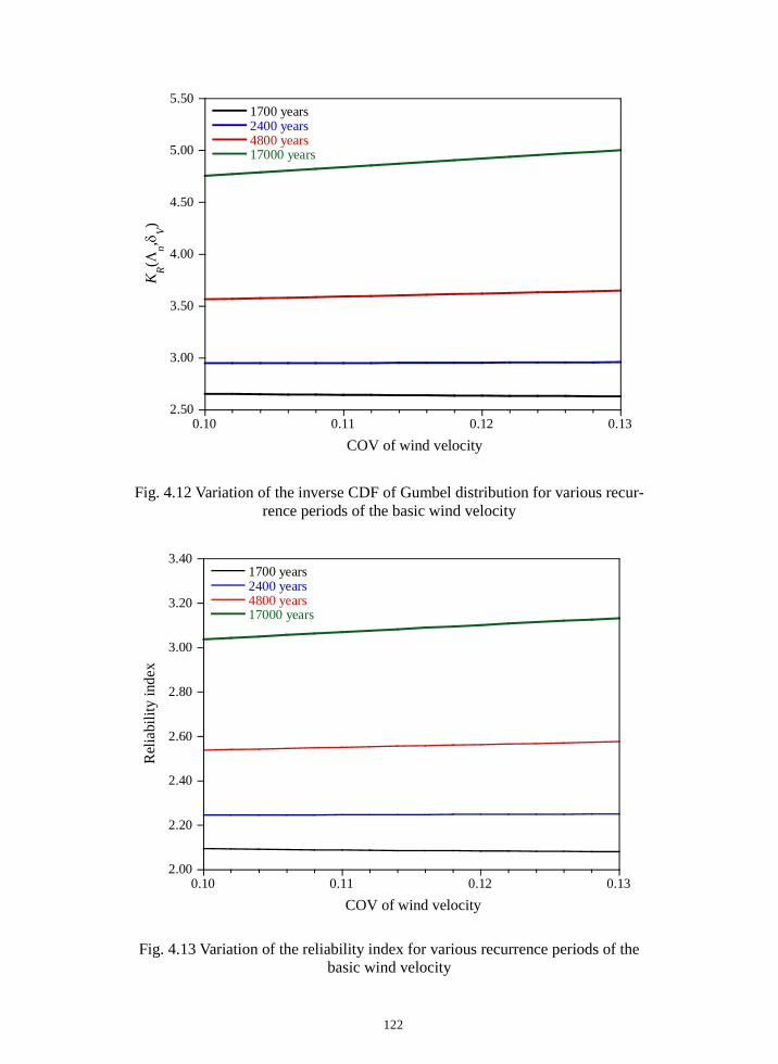
122

Fig. 4.12 Variation of the inverse CDF of Gumbel distribution for various recur-rence periods of the basic wind velocity

Fig. 4.13 Variation of the reliability index for various recurrence periods of the basic wind velocity

2.00

2.20

2.40

2.60

2.80

3.00

3.20

3.40

0.10 0.11 0.12 0.13

1700 years2400 years4800 years17000 years

Rel

iabi

lity

inde

x


2.50

3.00

3.50

4.00

4.50

5.00

5.50

0.10 0.11 0.12 0.13

1700 years2400 years4800 years17000 years

K R(Λn,δ

V)


123

4.3.2 Adjusted wind load factors and suggested wind velocity for KHBDC (LSD)

The adjustment procedure is applied for KHBDC (LSD) (KMOLIT, 2016a) in this

section. The results of the adjustment procedure for KHBDC (LSD) are presented

in Table 4.12 for βT = 3.1, δWS = 0.3. The wind load factors that satisfy the design

equation for KHBDC (LSD), are shown in Fig. 4.14 with centered symbols for the

three COVs and the target reliability indexes. The best-fit line for the wind load

factors marked with the centered symbols in Fig. 4.14 are drawn by 0.820 of the

adjustment factor, and plotted with lines in the figure. The adjusted wind load

factors for KHBDC (LSD) are summarized in Table 4.10 for the three COVs and

the target reliability indexes.

γWS = 0.82 λWS (1+ δWS Kgb(βT)) (4.22)

The dead load factors specified in the AASHTO specifications, KHBDC (LSD) are

presented in Table 4.8. Since the load factors of DC and DW in KHBDC (LSD)

are identical to the values in the AASHTO specifications, the discrepancy in (γWS )c

for the two design codes is caused by the difference of the design PMID of the py-

lons. In Tables 4.9 and 4.12, the ρAdj for the five bridges are identical to each oth-

er, and thus the nominal PMIDs for the two design codes coincide with each other

in P-M space. Therefore, the ratio of (γWS )C in the two tables becomes the ratio

of the design PMIDs of the AASHTO specifications and KHBDC (LSD), which is

calculated as 0.98. An equivalent resistance factor of the partial safety factors in

KHBDC (LSD) is estimated as 0.88 by multiplying the ratio of 0.98 by 0.90, which

is the resistance factor in the AASHTO specifications. The comparison of the

design PMID drawn by the two design codes is presented in Fig. 4.15 for the YSB

124

as a representative case for the five bridges.

The factored load effects of KHBDC (LSD) for the YSB are illustrated by

square symbols in Fig 4.7. The discrepancy in the adjusted wind load factors is

caused by the difference in the dead load factors of the two design codes. The

axial force induced by DC is greater than the compression due to DW, and the min-

imum load factor of DC for KHBDC (LSD)-CB is smaller than that for KHBDC

(LSD). Since the total factored dead load effects are obtained by multiplying the

dead load factor to the dead load effect, the total dead load effect for KHBDC

(LSD)-CB is located below those for KHBDC (LSD) in Fig. 4.7. The moment

capacity of a pylon increases rapidly as the compressive axial force increases in the

tensile failure region of the PMID. Therefore, the larger wind load factor is re-

quired for KHBDC (LSD) as the total factored load effect reaches the design PMID.

In KHBDC (LSD), the wind load factor is suggested as 1.4 but the target relia-

bility index is not specified in the code. The reliability level of KHBDC (LSD)

for the WGLS secured by the wind load factor is assessed. The bias factor of the

wind pressure for KHBDC (LSD) is written as follows by substituting Eq. (2.17)

into Eq. (4.22).

2

ˆ2

ˆ )()())(1(82.0

4.1 10

B

VqVq

TgbWSWS VK WSBWS

µµ=λµ=

βδ+=λ (4.23)

From Eq. (4.23), the standardized inverse CDF of the Gumbel distribution, Kgb(βT)

can be derived as follows.

WS

B

VqWS

Tgb

V

K

WS

δ−

µµδ

=γ+βΦ−π

−=β1

)(

707.1))))(ln((ln(6))(2

ˆ10

(4.24)

125

The reliability index is calculated as follows.

))))1

)(

707.1(6

exp((exp(2

ˆ

1

10

γ−δ

−µ

µδ

π−−Φ=β −

WS

B

VqWS VWS

(4.25)

The mean wind velocity, basic wind velocity, mean values of the normalized wind

pressure, and COV of the wind pressure are required to evaluate the reliability in-

dex for KHBDC (LSD) as shown in Eq. (4.25). The basic wind velocity in

KHBDC (LSD) is summarized in Table 4.13, and the mean value of 10V for 100-

year is presented in Table 2.8 for each region. However, the statistical parameters

of the normalized wind pressure given in Table 2.12 cannot be utilized since those

values are estimated using statistical parameters of the coefficients for wind pres-

sure valid for the long-span cable-supported bridges.

The statistical parameters of the coefficients for wind pressure are summarized

in Table 4.14 for short-to medium-span bridges. KHBDC (LSD) concerns only

the short- to medium-span bridges, of which the design is not required the wind

tunnel tests. The COV of the pressure coefficient is assumed as 0.12 because a

wind tunnel test is not performed, but the shape of a cross-section is roughly con-

sidered. The COV of the exposure coefficient is increased to 0.12 proposed by

Ellingwood et al. (1980) as a wind environment is not considered in KHBDC

(LSD).

Mote-Carlo simulations with 1 thousand trials are performed to determine the

distribution type of the normalized wind pressure for short- to medium-span bridg-

es. The fitness of the normalized wind pressure is confirmed by the Kolmogorov-

Smirnov goodness-of-fit test with a significance level of 0.01, and the empirical

CDF is constructed by the Weibull plotting positions. The statistical parameters

126

of the fitted Gumbel distribution for the normalized wind pressure are estimated

through Monte-Carlo simulations with 100 million trials. The cumulative proba-

bilities are plotted using the Gringorten plotting positions on the Gumbel probabil-

ity paper. The mean value of the normalized wind pressure and the bias factor

and COV of wind pressure are summarized in Table 4.14. The bias factor and

COV of wind pressure are calculated by Eq. (2.20) and Eq. (2.22), respectively.

The reliability indexes obtained by Eq. (4.25) are given in Table 4.14. The

basic wind velocity presented in KHBDC (LSD) secures the reliability level in the

rage of 2.15 to 3.51 for 4.1=γWS . The basic wind velocity in Category I results

in the reliability level of 2.15, while the reliability index in Category IV is calculat-

ed as 3.51. It is necessary to adjust the basic wind velocity in each Category in

order to secure a uniform reliability level. The basic wind velocity for a given

target reliability can be derived from Eq. (4.24) as follows.

)()910.1077.0(177.0

))(1(77.0

4.1))(1(82.0

1010

10

1010

ˆˆ

ˆˆ

TgbVV

qTgbqV

qTgbWSV

WS

qVB

K

K

KV

WSWS

WSWS

βδ++µ≈

µβδ+µ=

µβδ+µ=

λ

µµ=

(4.26)

By Eq. (4.26), the basic wind velocity can be determined based on the statistical

parameters of wind velocity without any information of structural characteristics

for short-to medium span bridges.

The suggested basic wind velocity for βT = 2.4, 2.8, and 3.1 are presented in

Table 4.15. The basic wind velocity in KHBDC (LSD) is also presented in the

table for comparison purposes. Since the wind load factor specified in KHBDC

(LSD) is smaller than the adjusted wind load factor presented in Table 4.10, the

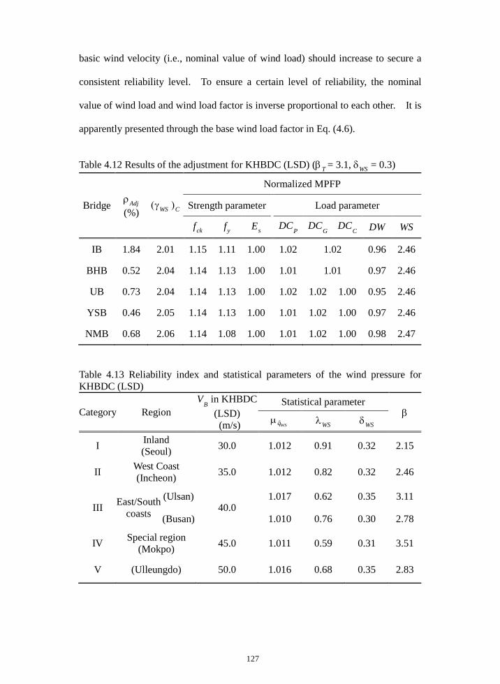
127

basic wind velocity (i.e., nominal value of wind load) should increase to secure a

consistent reliability level. To ensure a certain level of reliability, the nominal

value of wind load and wind load factor is inverse proportional to each other. It is

apparently presented through the base wind load factor in Eq. (4.6).

Table 4.12 Results of the adjustment for KHBDC (LSD) (βT = 3.1, δWS = 0.3)

Bridge ρAdj (%)

(γWS )C

Normalized MPFP



IB 1.84 2.01 1.15 1.11 1.00 1.02 1.02 0.96 2.46

BHB 0.52 2.04 1.14 1.13 1.00 1.01 1.01 0.97 2.46

UB 0.73 2.04 1.14 1.13 1.00 1.02 1.02 1.00 0.95 2.46

YSB 0.46 2.05 1.14 1.13 1.00 1.01 1.02 1.00 0.97 2.46

NMB 0.68 2.06 1.14 1.08 1.00 1.01 1.02 1.00 0.98 2.47

Table 4.13 Reliability index and statistical parameters of the wind pressure for KHBDC (LSD)

Category Region VB in KHBDC

(LSD) (m/s)

Statistical parameter β

WSqµ λWS δWS

I Inland (Seoul) 30.0 1.012 0.91 0.32 2.15

II West Coast (Incheon) 35.0 1.012 0.82 0.32 2.46

III East/South coasts

(Ulsan) 40.0

1.017 0.62 0.35 3.11

(Busan) 1.010 0.76 0.30 2.78

IV Special region (Mokpo) 45.0 1.011 0.59 0.31 3.51

V (Ulleungdo) 50.0 1.016 0.68 0.35 2.83

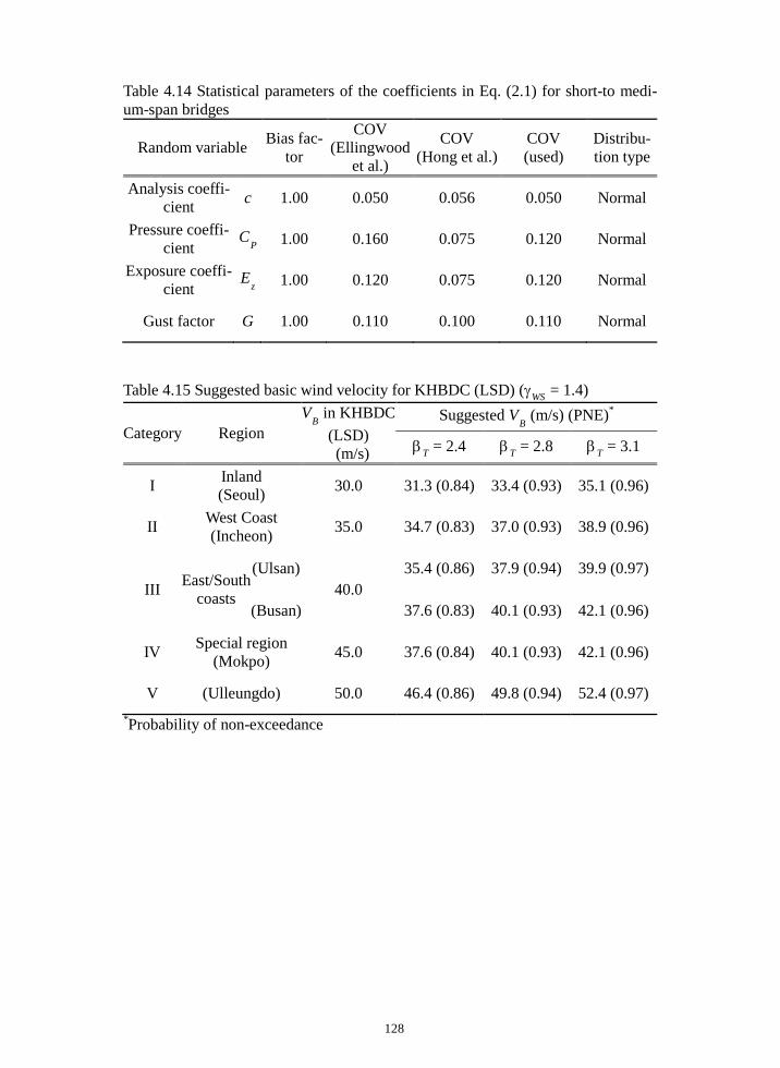
128

Table 4.14 Statistical parameters of the coefficients in Eq. (2.1) for short-to medi-um-span bridges

Random variable Bias fac-tor

COV (Ellingwood

et al.)

COV (Hong et al.)

COV (used)

Distribu-tion type

Analysis coeffi-cient c 1.00 0.050 0.056 0.050 Normal

Pressure coeffi-cient

CP 1.00 0.160 0.075 0.120 Normal

Exposure coeffi-cient

Ez 1.00 0.120 0.075 0.120 Normal

Gust factor G 1.00 0.110 0.100 0.110 Normal

Table 4.15 Suggested basic wind velocity for KHBDC (LSD) (γWS = 1.4)

Category Region VB in KHBDC

(LSD) (m/s)

Suggested VB (m/s) (PNE)*

βT = 2.4 βT = 2.8 βT = 3.1

I Inland (Seoul) 30.0 31.3 (0.84) 33.4 (0.93) 35.1 (0.96)

II West Coast (Incheon) 35.0 34.7 (0.83) 37.0 (0.93) 38.9 (0.96)

III East/South coasts

(Ulsan) 40.0

35.4 (0.86) 37.9 (0.94) 39.9 (0.97)

(Busan) 37.6 (0.83) 40.1 (0.93) 42.1 (0.96)

IV Special region (Mokpo) 45.0 37.6 (0.84) 40.1 (0.93) 42.1 (0.96)

V (Ulleungdo) 50.0 46.4 (0.86) 49.8 (0.94) 52.4 (0.97) *Probability of non-exceedance

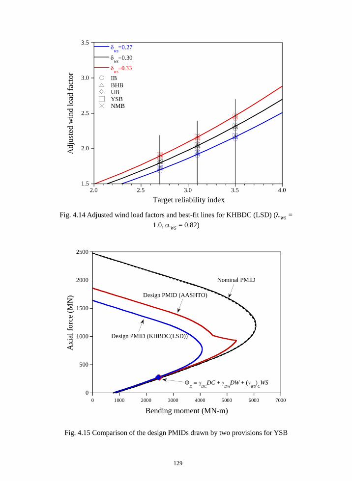
129

Fig. 4.14 Adjusted wind load factors and best-fit lines for KHBDC (LSD) (λWS = 1.0, αWS = 0.82)

Fig. 4.15 Comparison of the design PMIDs drawn by two provisions for YSB

1.5

2.0

2.5

3.0

3.5

2.0 2.5 3.0 3.5 4.0

δWS

=0.27

δWS

=0.30

δWS

=0.33

IBBHBUBYSBNMB

Adj

uste

d w

ind

load

fact

or


0

500

1000

1500

2000

2500

0 1000 2000 3000 4000 5000 6000 7000

Axi

al fo

rce

(MN

)


Design PMID (AASHTO)

Design PMID (KHBDC(LSD))

Nominal PMID

ΦD = γ

DCDC + γ

DWDW + (γ

WS)

CWS

130

4.4 Verification for Variations of Cross-sections

In the previous sections, the validity of the adjusted wind load factors is demon-

strated by adjusting the reinforcement ratio of the cross-section for the pylons.

However, the actual strength of RC columns depends on not only the reinforcement

ratio but the material and geometric properties of the section. The validity of the

adjusted wind load factor for various sizes of cross-sections and material properties

is required to confirm a general applicability of the wind load factor. It is difficult

to arbitrarily change the material properties for determining strength of RC col-

umns, since the material properties are generally specific to the materials and de-

pend on manufacturing processes and temperature. Therefore, the strength of RC

columns is determined by adjusting the geometric properties rather than material

properties to verify the adjusted wind load factor in this study. Choi (2016) pro-

posed a method for determining a cross-section to secure a target reliability level

for a given reinforcement ratio. In the proposed method, the geometric properties

are adjusted to obtain the strength of RC columns and the material properties of the

cross-section are maintained. The work by Choi (2016) is adopted to determine

the cross-section of RC pylons, and the applicability of the proposed wind load

factor is demonstrated through the various sizes of the cross-section.

In Section 4.4.1, detail procedures for determining a cross-section, which yields

the target reliability index for a given reinforcement ratio, are presented. In Sec-

tion 4.4.2, the proposed wind load factors are verified through the optimum section

of the pylons.

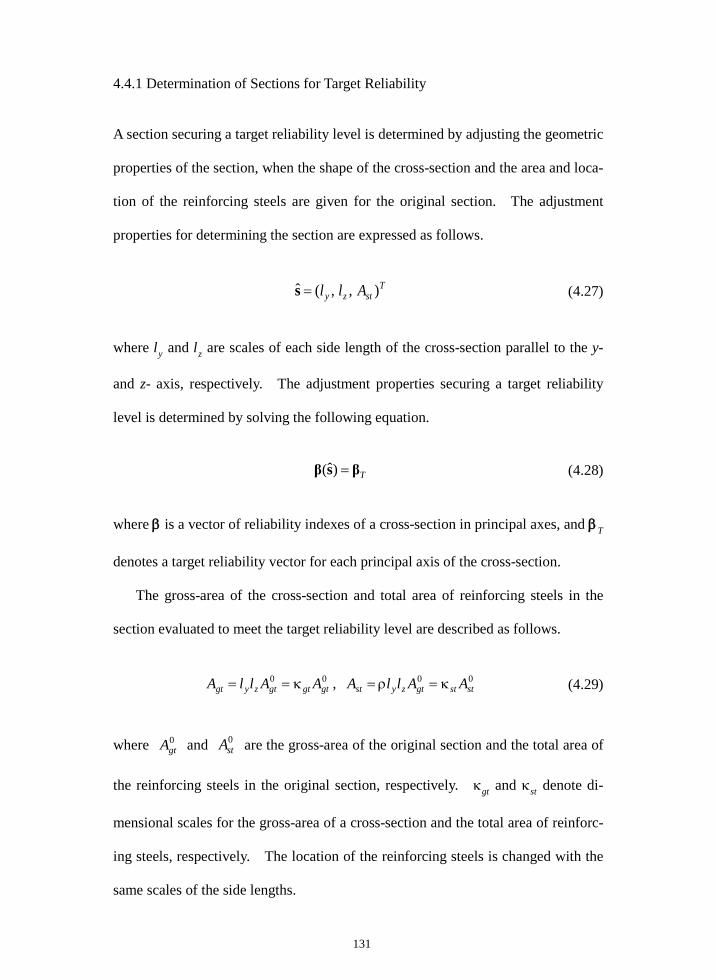
131

4.4.1 Determination of Sections for Target Reliability

A section securing a target reliability level is determined by adjusting the geometric

properties of the section, when the shape of the cross-section and the area and loca-

tion of the reinforcing steels are given for the original section. The adjustment

properties for determining the section are expressed as follows.

T

stzy All ),,(ˆ =s (4.27)

where ly and lz are scales of each side length of the cross-section parallel to the y-

and z- axis, respectively. The adjustment properties securing a target reliability

level is determined by solving the following equation.

Tβsβ =)ˆ( (4.28)

where β is a vector of reliability indexes of a cross-section in principal axes, and βT

denotes a target reliability vector for each principal axis of the cross-section.

The gross-area of the cross-section and total area of reinforcing steels in the

section evaluated to meet the target reliability level are described as follows.

00gtgtgtzygt AAllA κ== , 00

ststgtzyst AAllA κ=ρ= (4.29)

where 0gtA and 0

stA are the gross-area of the original section and the total area of

the reinforcing steels in the original section, respectively. κgt and κst denote di-

mensional scales for the gross-area of a cross-section and the total area of reinforc-

ing steels, respectively. The location of the reinforcing steels is changed with the

same scales of the side lengths.

132

The different reliability indexes are obtained for each principal axis because the

cross-section of a pylon is generally asymmetric, and the external loads generate

different magnitudes of the load effect to the principal axes. The strength of

cross-sections can be determined to satisfy the target reliability index for either two

principal axes or one axis corresponding to the lowest reliability index. In order

to ascertain the target reliability index for the two axes, it is necessary to change

side lengths of the section parallel to the x- and y-axis separately. In order to de-

termine the cross-section at which the lowest reliability index reaches the target

reliability index, the lengths of each side are assumed to be change with the same

scale, ly = lz.

The equation given in Eq. (4.27) cannot be solved because the number of equa-

tions is smaller than that of the unknowns (i.e., the adjustment properties). There-

fore, an additional condition is required to solve the equation, and the number of an

additional condition is equal to that of deficient equations. The additional condi-

tion may be introduced by a regularization function to define Eq. (4.27) as an opti-

mization problem. However, it is not easy to logically determine the regulariza-

tion factor in solving the optimization problem. In this study, Eq. (4.27) is direct-

ly solved by utilizing the reinforcement ratio as the additional condition. The

cross-section satisfying the target reliability index is founded by determining the

gross-area of the cross-section for a given reinforcement ratio, and Tzy ll ),(ˆ =s .

Since the reliability index is nonlinear with respect to the adjustment properties, an

iterative procedure based on the Newton-Raphson method is employed to solve Eq.

(4.27).

133

Tkkk

βssβsβsβ

s=∆

∂∂

+≈+ ˆˆ

)ˆ()ˆ()ˆ(

1 (4.30)

where subscript k denotes the iteration count, and sss ˆˆˆ 1 ∆+=+ kk . The solution

of Eq. (4.30) yields the expression of s∆ .

))ˆ(()ˆ

(ˆ 1kT sββ

sβs −

∂∂

=∆ − (4.31)

The sensitivity of the reliability index with respect to the adjustment properties is

approximated by the finite difference method.

12

12

)ˆ()ˆ()()(

ˆˆ jj

ii

j

i

j

i

ssss −β−β

=∆

β∆≈

∂β∂ , for zyi ,= (4.32)

where js indicates the j-th component of the adjustment properties, and

jjj sss ˆ)ˆ()ˆ( 12 ∆+= . (β i)1 and (β i)2 are the reliability indexes for the i-directional

axis obtained by 1)ˆ( js and 2)ˆ( js , respectively. y and z represent the principal

axes of a cross-section. The proper step size, js∆ , is selected to obtain stable,

converged, and consistent solutions in the finite difference approach.

The change in the size of the cross-sections causes the change in the stiffness of

the column. For the sake of simplicity, a change in the stiffness due to the varia-

tion of the cross-section is neglected, and changes in the strength of the RC column

used in constructing the PMID are considered. Load effects as well as the

strength of an RC column are affected by a change in the gross-area of the cross-

section. The variation of the load effects according to the change of the cross-

section is also considered in determining the cross-section. The load effect in-

134

duced by the self-weight of a column is directly proportional to the gross-area of

the cross-section of the column. The load effect due to the lateral load is propor-

tional to the side length of the cross-section, which is perpendicular to the direction

of the lateral load.

4.4.2 Verifications of Wind Load Factors

The RC pylons for IB and UB are utilized to verify the adjusted wind load factors

for KHBDC (LSD)-CB (KMOLIT, 2016b), and the pylon section of each bridge is

adjusted to secure a target reliability level. The cross-section determined to yield

a target reliability index is refer referred to as an adjusted section in this study.

The adjusted section of IB and UB is designed so that the lowest reliability index

of the adjusted section meets the target reliability index of 3.1 which is specified in.

KHBDC (LSD)-CB. The stress-strain relationships of concrete and reinforcing

steels in KHBDC (LSD) (KMOLIT, 2016a) are utilized to construct the PMIDs of

the pylon sections, and the design PMID is obtained by using the partial safety fac-

tors of concrete and reinforcing steels specified in KHBDC (LSD).

The basic wind velocities for KHBDC (LSD)-CB is presented in Table 4.16 for

IB and UB, and the bias factor and probability of non-exceedance of the basic wind

velocity are summarized in the table. The statistical parameters of wind pressure

are presented in Table 4.16. The bias factor of wind pressure corresponding to the

basic wind velocity is calculated by Eq. (2.20), and the COV of the wind pressure

is quoted from Table 2.11. In Table 4.17, the wind load effects due to the basic

wind velocity are summarized in case that the wind pressure corresponding to the

basic wind velocities act on each bridge in WD2. In the table, individual load

effects generated by the wind load acting on the pylon and the other members are

135

summarized for IB and UB. The wind load effects in Table 4.17 and the dead

load effects given in Table 3.5 are utilized in determining the adjusted section.

The change in the magnitude of the dead and wind load effects according to the

variation of the cross-section is considered in determining an adjusted section.

The random variables include the load parameters and the geometric and material

properties, and their statistical parameters are given in Table 3.2.

Fig. 4.16 shows the variation of the dimensional scales for the adjusted sections

of the given reinforcement ratios for IB and UB. The reinforcement ratio varies

from 0.01 to 0.04 at intervals of 0.005 for the two bridges. For the reinforcement

ratio of 0.04 for IB, of which value is close to that of the original section, the gross-

area of the cross-section decreases about 60% so as to satisfy the target reliability

index. On the other hand, if the gross-area of the cross-section is maintained that

of the original section, the reinforcement ratio of the adjusted section is calculated

as 0.02 to yield the target reliability level. The adjusted section for 4% of the re-

inforcement ratio is illustrated in Fig. 4.17 as the representative case of the adjusted

sections, and the results of the reliability assessment for the adjusted section are

presented in Table 4.18 and Fig. 4.18. The reinforcement ratio of the adjusted

section for UB is calculated 0.01 in case that the gross-are of the adjusted section is

equal to that of the original section. Meanwhile, the gross-area of the cross-

section for UB is reduced to 68 % for the adjusted section in which the reinforce-

ment ratio is given as 0.02. The adjusted section for the reinforcement ratio of 2%

is presented in Fig. 4.19, and the PMIDs and failure points obtained from the relia-

bility analysis are drawn in Fig. 4.20. The reliability index and normalized

MPFPs are summarized in Table 4.18. It is shown that the adjusted section is de-

termined to secure the target reliability level within an 1% error.

136

The design PMIDs of the adjusted sections and the total factored load effect for

IB and UB are illustrated in Fig. 4.21 for various reinforcement ratios. The total

factored load effect is obtained by the dead load factors in KHBDC (LSD)-CB and

the adjusted wind load factors. The adjusted wind load factors are calculated as

2.18 and 2.38 for IB and UB by substituting the statistical parameters of the wind

pressure in Table 4.16 into Eq. 4.12. The total factored load effect is located very

close to the design PMID regardless of the reinforcement ratio, in other words, the

size of the cross-section. The required and adjusted wind load factors are summa-

rized in Table 4.19 for the given reinforcement ratios. The wind load factor,

which allows the total factored load effects to be exactly located on the design

PMID in Fig. 4.21, is referred to as the required wind load factor. The errors be-

tween the required and adjusted wind load factors are calculated less than 2.8%.

It is definitely seen that the design equation and the adjustment procedure are

available for the changes in the cross-section.

Table 4.16 Basic wind velocity and pressure, its statistical characteristics

Bridge VB Bias factor of

VB Probability of Non-

exceedance of VB (%) Bias factor

of wind pressure

COV of wind pres-

sure

IB 29.9 1.05 36.60

1.12 0.2880

UB 29.4 1.06 1.15 0.3216

Table 4.17 Composition of wind load effects

Bridge Total wind load effect (WS) WSP WSetc

IB Pq (MN) -52.59 -20.91 -31.68

Mq (MN·m) 712.91 352.71 360.20

UB Pq (MN) -49.29 -19.72 -29.58

Mq (MN·m) 251.37 123.17 128.20

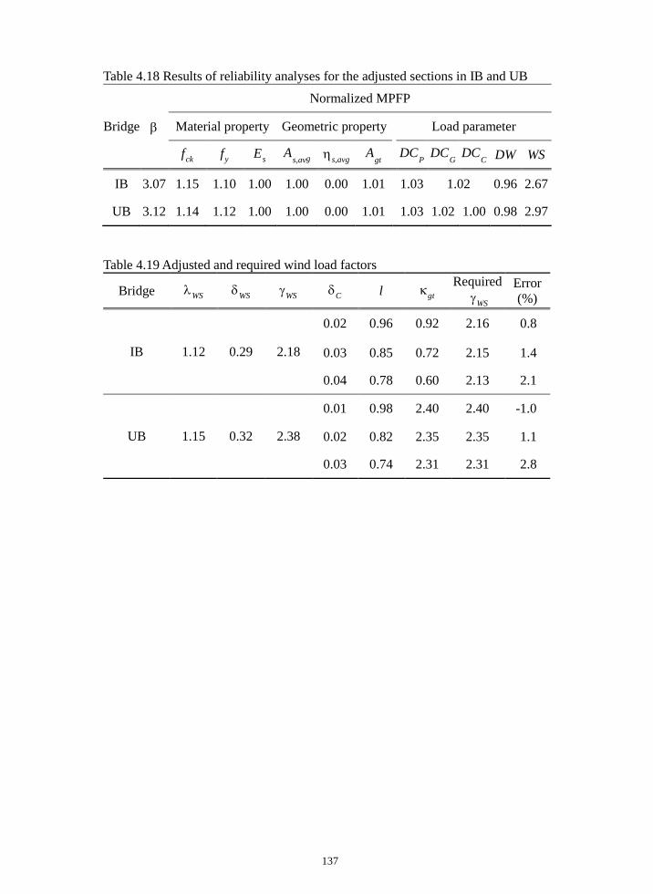
137

Table 4.18 Results of reliability analyses for the adjusted sections in IB and UB

Bridge β

Normalized MPFP


fck fy Es As,avg ηs,avg Agt DCP DCG DCC DW WS

IB 3.07 1.15 1.10 1.00 1.00 0.00 1.01 1.03 1.02 0.96 2.67

UB 3.12 1.14 1.12 1.00 1.00 0.00 1.01 1.03 1.02 1.00 0.98 2.97

Table 4.19 Adjusted and required wind load factors

Bridge λWS δWS γWS δC l κgt Required

γWS Error (%)

IB 1.12 0.29 2.18

0.02 0.96 0.92 2.16 0.8

0.03 0.85 0.72 2.15 1.4

0.04 0.78 0.60 2.13 2.1

UB 1.15 0.32 2.38

0.01 0.98 2.40 2.40 -1.0

0.02 0.82 2.35 2.35 1.1

0.03 0.74 2.31 2.31 2.8

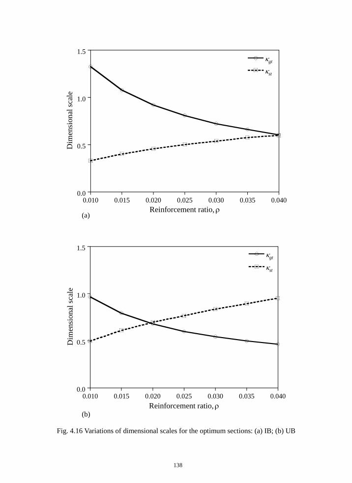
138

(a) (b)

Fig. 4.16 Variations of dimensional scales for the optimum sections: (a) IB; (b) UB

0.0

0.5

1.0

1.5

0.010 0.015 0.020 0.025 0.030 0.035 0.040

κgt

κstD

imen

sion

al sc

ale

Reinforcement ratio, ρ

0.0

0.5

1.0

1.5

0.010 0.015 0.020 0.025 0.030 0.035 0.040

κgt

κst

Dim

ensi

onal

scal

e

Reinforcement ratio, ρ

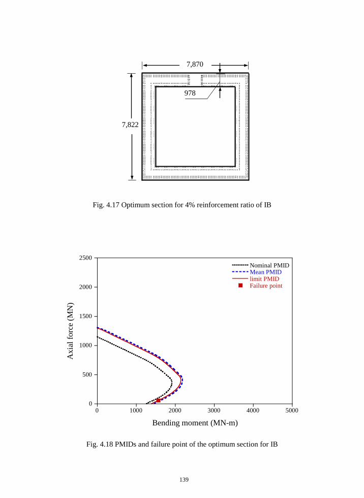
139

Fig. 4.17 Optimum section for 4% reinforcement ratio of IB

Fig. 4.18 PMIDs and failure point of the optimum section for IB

7,870

7,822

978

0

500

1000

1500

2000

2500

0 1000 2000 3000 4000 5000

Nominal PMIDMean PMIDlimit PMIDFailure point

Axi

al fo

rce

(MN

)


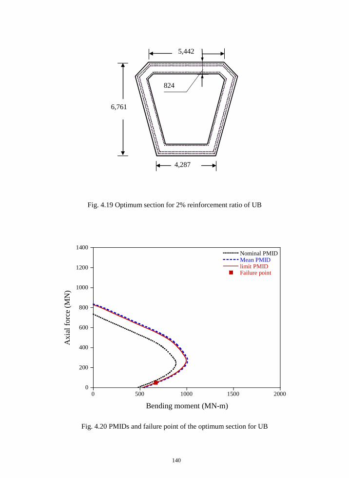
140

Fig. 4.19 Optimum section for 2% reinforcement ratio of UB

Fig. 4.20 PMIDs and failure point of the optimum section for UB

0

200

400

600

800

1000

1200

1400

0 500 1000 1500 2000

Nominal PMIDMean PMIDlimit PMIDFailure point

Axi

al fo

rce

(MN

)


6,761

4,287

5,442

824

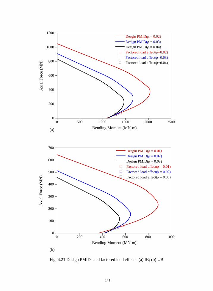
141

(a)

(b)

Fig. 4.21 Design PMIDs and factored load effects: (a) IB; (b) UB

0

200

400

600

800

1000

1200

0 500 1000 1500 2000 2500

Desgin PMID(ρ = 0.02)Design PMID(ρ = 0.03)Design PMID(ρ = 0.04)Factored load effect(ρ=0.02)Factored load effect(ρ=0.03)Factored load effect(ρ=0.04)

Axi

al F

orce

(MN

)

Bending Moment (MN-m)

0

100

200

300

400

500

600

700

0 200 400 600 800 1000

Desgin PMID(ρ = 0.01)Design PMID(ρ = 0.02)Design PMID(ρ = 0.03)Factored load effect(ρ = 0.01)Factored load effect(ρ = 0.02)Factored load effect(ρ = 0.03)

Axi

al F

orce

(MN

)

Bending Moment (MN-m)

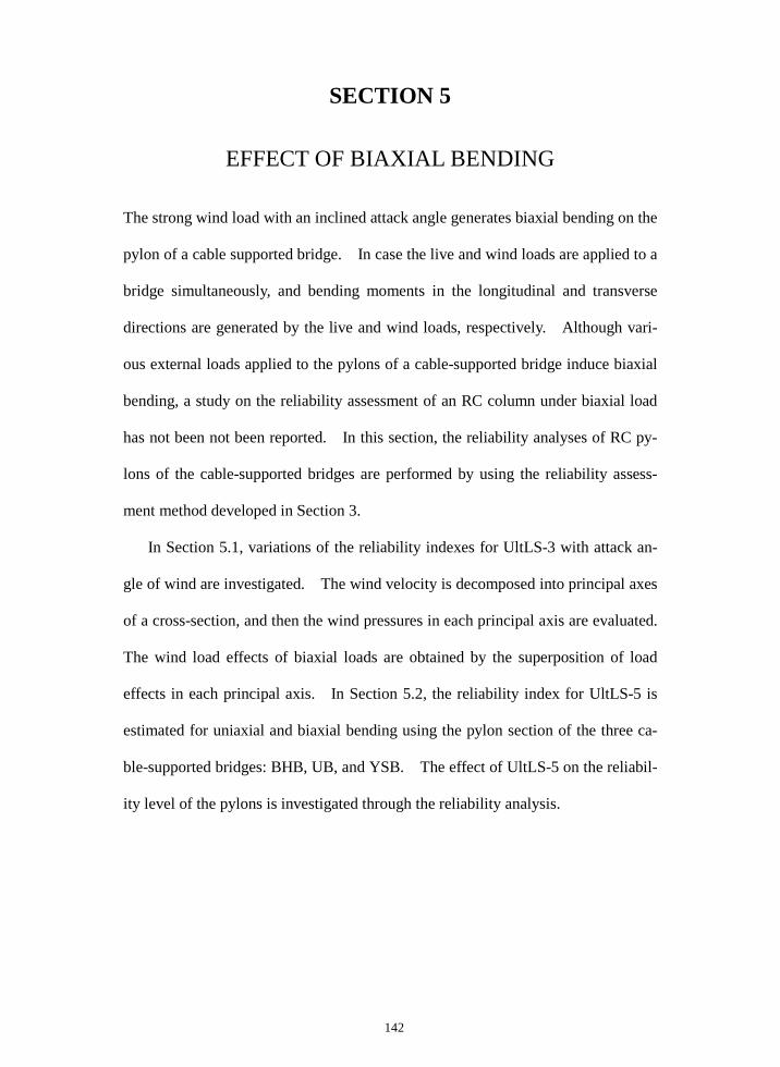
142

SECTION 5

EFFECT OF BIAXIAL BENDING

The strong wind load with an inclined attack angle generates biaxial bending on the

pylon of a cable supported bridge. In case the live and wind loads are applied to a

bridge simultaneously, and bending moments in the longitudinal and transverse

directions are generated by the live and wind loads, respectively. Although vari-

ous external loads applied to the pylons of a cable-supported bridge induce biaxial

bending, a study on the reliability assessment of an RC column under biaxial load

has not been not been reported. In this section, the reliability analyses of RC py-

lons of the cable-supported bridges are performed by using the reliability assess-

ment method developed in Section 3.

In Section 5.1, variations of the reliability indexes for UltLS-3 with attack an-

gle of wind are investigated. The wind velocity is decomposed into principal axes

of a cross-section, and then the wind pressures in each principal axis are evaluated.

The wind load effects of biaxial loads are obtained by the superposition of load

effects in each principal axis. In Section 5.2, the reliability index for UltLS-5 is

estimated for uniaxial and biaxial bending using the pylon section of the three ca-

ble-supported bridges: BHB, UB, and YSB. The effect of UltLS-5 on the reliabil-

ity level of the pylons is investigated through the reliability analysis.

143

5.1 Reliability Assessment of RC Pylons under Biaxial Bending for UltLS-3

The angle of attack for wind load to an RC pylon, θWS, is illustrated in Fig. 3.9.

The angle of θWS = 0°, 90°, 180° and 270° indicate WD1, WD2, WD3, and WD4,

respectively. For each wind load direction, the load effects induced by the mean

wind pressure are presented in Tables 4.3 and 4.4. The biaxial load effects are

obtained by the superposition of the load effect in each direction for the reliability

analyses. The reinforcement ratios of the cross-section presented in Table 4.6 are

used for the strength of the pylons. The strength obtained by the reinforcement

ratio in the table yields the lowest reliability index to the target reliability index of

3.1 for λWS = 1, δWS = 0.3.

The load parameters and the geometric and material properties are considered

as random variables, and their statistical parameters are presented in Table 3.2.

The reliability analyses are conducted for the surface exponents of 2 and 1. The

angle of attack for wind load varies from 0° to 360° while the nominal magnitude

of the wind load is maintained constant. For α = 2, the reliability analysis is per-

formed with an interval of 5° for the angle of attack of wind load. The interval for

the angle of attack for α = 1 is defined as 1° in order to illustrate variations of the

reliability indexes later on the figures.

The minimum reliability index for α = 2 is equal to 3.1 for all bridges, while

those for α = 1 are calculated as various levels as shown in Table 5.1. The mini-

mum reliability index for each pylon varies from 2.22 to 2.98. The difference of

the minimum reliability index with the target reliability of 3.1 is presented 28% for

BHB, which exhibits very large compared to those of the other bridges. It is be-

144

cause that the wind load for BHB induces large bending moments in both the

transverse and longitudinal directions in contrast with those for the other bridges.

The minimum reliability index for the UB, YSB and NMB is calculated at similar

angles of attack for wind load, which implies that the failure of the three suspen-

sion bridges occurs with similar tendencies by wind load. In the five bridges, the

minimum reliability indexes for biaxial bending are lower than the target reliability

of 3.1 by 4% to 28%. It is noted that a significantly lower reliability level may be

secured for biaxial bending, even if a pylon secures a high reliability level for uni-

axial bending.

The results of the reliability assessment for biaxial load are presented in Figs.

5.1 and 5.2 for IB. Fig. 5.1 and Fig. 5.2 show variations of the reliability indexes

and the standard normal wind load at the MPFP for IB, respectively. The varia-

tion patterns of the two figures are quite similar to each other, which implies that

the wind load governs the failure of the pylon for the biaxial loads. The reliability

levels of α = 2 are higher than the target reliability level for all the angle of attack.

The lowest reliability index of α = 1 is calculated as 2.98 at the angle of attack of

106° and is 4% smaller than the target reliability index of 3.1. The reliability in-

dexes of α = 1 are smaller than those of α = 2 for all angles of attack because the

strength obtained by the load contour for α = 1 is determined much smaller than

that for α = 2.

Fig. 5.3 shows the nominal load effects and failure points for IB are marked

with centered symbols for 3600 ≤θ≤ WS . In the figure, the nominal load ef-

fects and failure points for α = 2 are marked with centered symbols every 5°, and

failure points for α =1 are presented every 1° in the counter-clockwise direction.

145

The solid squares in the figure indicate the internal forces at φ = 0°, while the solid

circles are associated with θWS = 90°, 180° and 270°. The axial forces corre-

sponding to each centered symbol are different, and the load effects are located on

different My-Mz planes in 3D space. The wind loads acting on the pylon in WD2

and WD4 generate the bending moments in the opposite and same directions to the

bending moment due to the dead load, respectively, and thus the positions of the

black circles representing the nominal load effects are located above the axis of My

= 0.

The results clearly show that the angles of attack for the failure points on the

moment axes in Fig. 5.3 exactly coincide with those where the discontinuities of α

= 1 and are observed in Figs. 5.1 and 5.2. The reliability index of the pylon is

calculated for uniaxial bending corresponding to θWS = 0°, 90°, 180° and 270° and

is compared with that for biaxial bending in Table 5.2. A slight difference in the

reliability indexes between uniaxial and biaxial loads is caused by the biaxial mo-

ment due to the dead load.

The wind loads in WD2 and WD4 induce the tensile and compressive axial

forces, respectively. The moment capacity of a pylon decreases rapidly as the

compressive axial force diminishes in the tensile failure region of the PMID, which

is clearly observed in Figs. 3.9-3.13. Therefore, the load effects in WD4 yield a

higher level of safety than the reliability level of WD2 even though the total nomi-

nal moment in WD4 exhibits larger than that in WD2. As in the transverse wind

load case, the difference in the reliability indexes for the longitudinal directions

(WD1 and WD3) is caused by the direction of axial force due to wind load. Since,

the axial force induced by the longitudinal wind load is 0.3% of the total axial force,

the difference in axial forces for WD1 and WD3 has little effect on the reliability

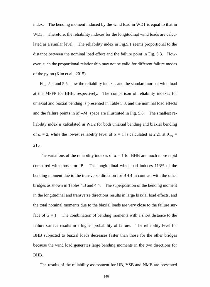
146

index. The bending moment induced by the wind load in WD1 is equal to that in

WD3. Therefore, the reliability indexes for the longitudinal wind loads are calcu-

lated as a similar level. The reliability index in Fig.5.1 seems proportional to the

distance between the nominal load effect and the failure point in Fig. 5.3. How-

ever, such the proportional relationship may not be valid for different failure modes

of the pylon (Kim et al., 2015).

Figs 5.4 and 5.5 show the reliability indexes and the standard normal wind load

at the MPFP for BHB, respectively. The comparison of reliability indexes for

uniaxial and biaxial bending is presented in Table 5.3, and the nominal load effects

and the failure points in My–Mz space are illustrated in Fig. 5.6. The smallest re-

liability index is calculated in WD2 for both uniaxial bending and biaxial bending

of α = 2, while the lowest reliability level of α = 1 is calculated as 2.21 at θWS =

215°.

The variations of the reliability indexes of α = 1 for BHB are much more rapid

compared with those for IB. The longitudinal wind load induces 113% of the

bending moment due to the transverse direction for BHB in contrast with the other

bridges as shown in Tables 4.3 and 4.4. The superposition of the bending moment

in the longitudinal and transverse directions results in large biaxial load effects, and

the total nominal moments due to the biaxial loads are very close to the failure sur-

face of α = 1. The combination of bending moments with a short distance to the

failure surface results in a higher probability of failure. The reliability level for

BHB subjected to biaxial loads decreases faster than those for the other bridges

because the wind load generates large bending moments in the two directions for

BHB.

The results of the reliability assessment for UB, YSB and NMB are presented

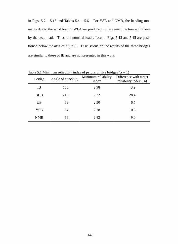
147

in Figs. 5.7 – 5.15 and Tables 5.4 – 5.6. For YSB and NMB, the bending mo-

ments due to the wind load in WD4 are produced in the same direction with those

by the dead load. Thus, the nominal load effects in Figs. 5.12 and 5.15 are posi-

tioned below the axis of My = 0. Discussions on the results of the three bridges

are similar to those of IB and are not presented in this work.

Table 5.1 Minimum reliability index of pylons of five bridges (α = 1)

Bridge Angle of attack (°) Minimum reliability index

Difference with target reliability index (%)

IB 106 2.98 3.9

BHB 215 2.22 28.4

UB 69 2.90 6.5

YSB 64 2.78 10.3

NMB 66 2.82 9.0

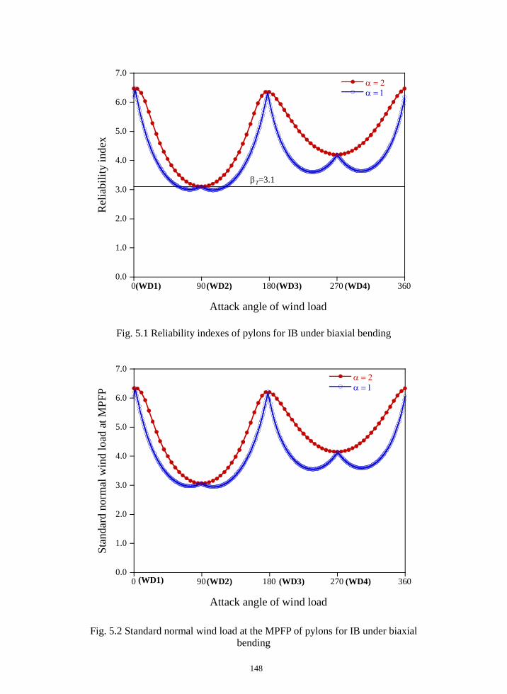
148

Fig. 5.1 Reliability indexes of pylons for IB under biaxial bending

Fig. 5.2 Standard normal wind load at the MPFP of pylons for IB under biaxial bending

0.0

1.0

2.0

3.0

4.0

5.0

6.0

7.0

0 90 180 270 360

α = 2α = 1

Rel

iabi

lity

inde

x

Attack angle of wind load

βT=3.1

(WD2)(WD1) (WD3) (WD4)

0.0

1.0

2.0

3.0

4.0

5.0

6.0

7.0

0 90 180 270 360

α = 2α = 1

Stan

dard

nor

mal

win

d lo

ad a

t MPF

P


(WD1) (WD2) (WD3) (WD4)

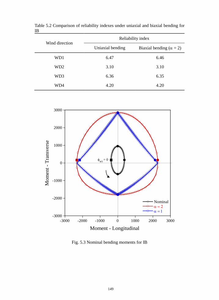
149

Table 5.2 Comparison of reliability indexes under uniaxial and biaxial bending for IB

Wind direction Reliability index

Uniaxial bending Biaxial bending (α = 2)

WD1 6.47 6.46

WD2 3.10 3.10

WD3 6.36 6.35

WD4 4.20 4.20

Fig. 5.3 Nominal bending moments for IB

-3000

-2000

-1000

0

1000

2000

3000

-3000 -2000 -1000 0 1000 2000 3000

Nominal α = 2α = 1

Mom

ent -

Tra

nsve

rse

Moment - Longitudinal

φWS

= 0

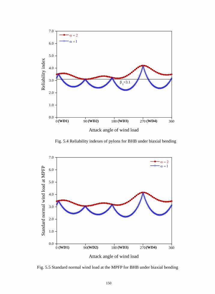
150

Fig. 5.4 Reliability indexes of pylons for BHB under biaxial bending

Fig. 5.5 Standard normal wind load at the MPFP for BHB under biaxial bending

0.0

1.0

2.0

3.0

4.0

5.0

6.0

7.0

0 90 180 270 360

α = 2

α = 1R

elia

bilit

y in

dex


βT=3.1

(WD1) (WD2) (WD3) (WD4)

0.0

1.0

2.0

3.0

4.0

5.0

6.0

7.0

0 90 180 270 360

α = 2α = 1

Stan

dard

nor

mal

win

d lo

ad a

t MPF

P


(WD1) (WD2) (WD3) (WD4)

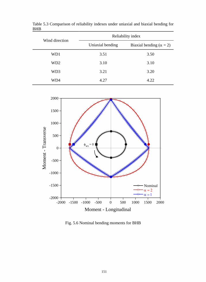
151

Table 5.3 Comparison of reliability indexes under uniaxial and biaxial bending for BHB



WD1 3.51 3.50

WD2 3.10 3.10

WD3 3.21 3.20

WD4 4.27 4.22

Fig. 5.6 Nominal bending moments for BHB

-2000

-1500

-1000

-500

0

500

1000

1500

2000

-2000 -1500 -1000 -500 0 500 1000 1500 2000


Mom

ent -

Tra

nsve

rse


φWS

= 0

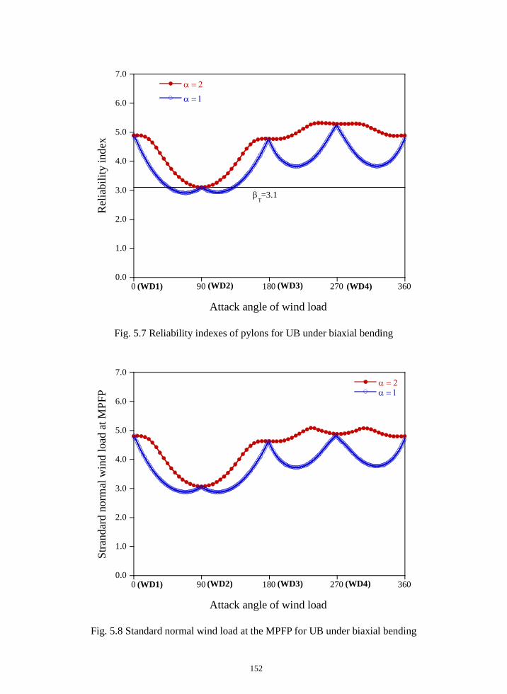
152

Fig. 5.7 Reliability indexes of pylons for UB under biaxial bending

Fig. 5.8 Standard normal wind load at the MPFP for UB under biaxial bending

0.0

1.0

2.0

3.0

4.0

5.0

6.0

7.0

0 90 180 270 360

α = 2

α = 1R

elia

bilit

y in

dex


βT=3.1

(WD1) (WD2) (WD3) (WD4)

0.0

1.0

2.0

3.0

4.0

5.0

6.0

7.0

0 90 180 270 360

α = 2α = 1

Stra

ndar

d no

rmal

win

d lo

ad a

t MPF

P


(WD1) (WD2) (WD3) (WD4)

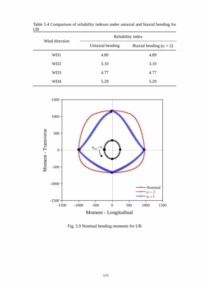
153

Table 5.4 Comparison of reliability indexes under uniaxial and biaxial bending for UB



WD1 4.89 4.89

WD2 3.10 3.10

WD3 4.77 4.77

WD4 5.29 5.29

Fig. 5.9 Nominal bending moments for UB

-1500

-1000

-500

0

500

1000

1500

-1500 -1000 -500 0 500 1000 1500


Mom

ent -

Tra

nsve

rse


φWS

= 0

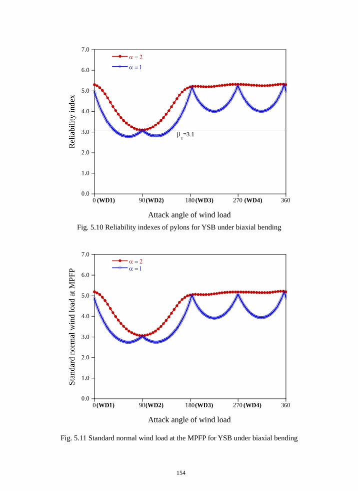
154

Fig. 5.10 Reliability indexes of pylons for YSB under biaxial bending

Fig. 5.11 Standard normal wind load at the MPFP for YSB under biaxial bending

0.0

1.0

2.0

3.0

4.0

5.0

6.0

7.0

0 90 180 270 360

α = 2

α = 1R

elia

bilit

y in

dex


βT=3.1

(WD1) (WD2) (WD3) (WD4)

0.0

1.0

2.0

3.0

4.0

5.0

6.0

7.0

0 90 180 270 360

α = 2α = 1

Stan

dard

nor

mal

win

d lo

ad a

t MPF

P


(WD1) (WD2) (WD3) (WD4)

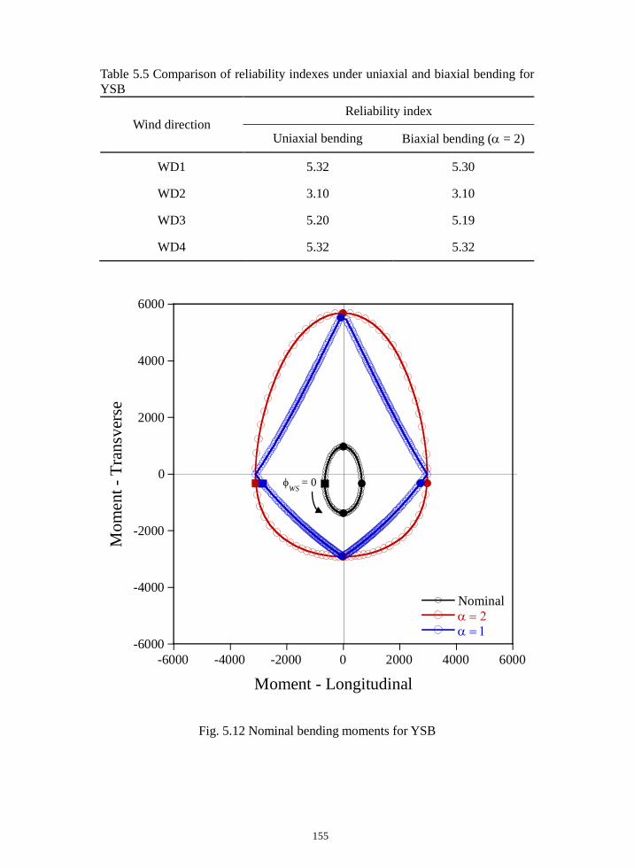
155

Table 5.5 Comparison of reliability indexes under uniaxial and biaxial bending for YSB



WD1 5.32 5.30

WD2 3.10 3.10

WD3 5.20 5.19

WD4 5.32 5.32

Fig. 5.12 Nominal bending moments for YSB

-6000

-4000

-2000

0

2000

4000

6000

-6000 -4000 -2000 0 2000 4000 6000


Mom

ent -

Tra

nsve

rse


φWS

= 0

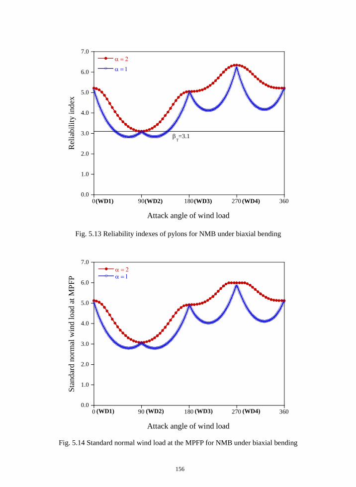
156

Fig. 5.13 Reliability indexes of pylons for NMB under biaxial bending Fig. 5.14 Standard normal wind load at the MPFP for NMB under biaxial bending

0.0

1.0

2.0

3.0

4.0

5.0

6.0

7.0

0 90 180 270 360

α = 2

α = 1R

elia

bilit

y in

dex


βT=3.1

(WD1) (WD2) (WD3) (WD4)

0.0

1.0

2.0

3.0

4.0

5.0

6.0

7.0

0 90 180 270 360

α = 2α = 1

Stan

dard

nor

mal

win

d lo

ad a

t MPF

P


(WD1) (WD2) (WD3) (WD4)

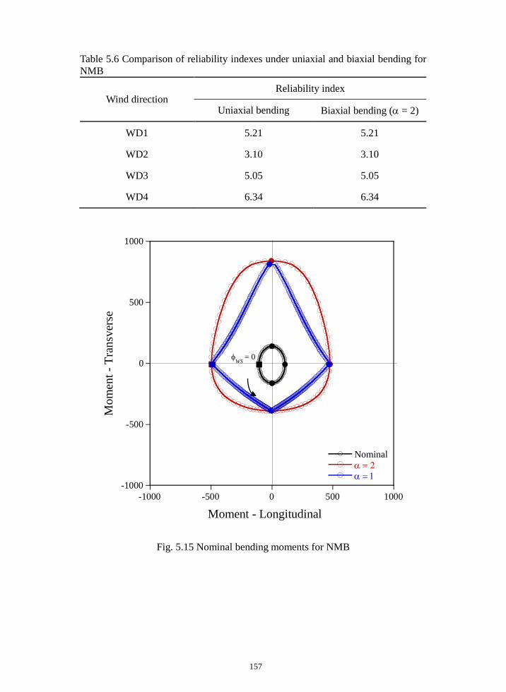
157

Table 5.6 Comparison of reliability indexes under uniaxial and biaxial bending for NMB



WD1 5.21 5.21

WD2 3.10 3.10

WD3 5.05 5.05

WD4 6.34 6.34

Fig. 5.15 Nominal bending moments for NMB

-1000

-500

0

500

1000

-1000 -500 0 500 1000


Mom

ent -

Tra

nsve

rse


φWS

= 0

158

5.2 Reliability Assessment of RC Pylons under Biaxial Bending for UltLS-5

The design specifications and codes define a load combination for wind load that

allows vehicular live loads, which is referred to as UltLS-5 in KHBDC (LSD)-CB

(KMOLIT, 2016b). In KHBDC (LSD)-CB, the wind velocity at which normal

vehicular traffics are allowed is limited to V10 = 25 m/s. Tables 5.7 and 5.8 show

the load effects corresponding to UltLS-5 at the bottom section of the pylon. In

the table, WS25 and LL indicate the wind load corresponding to V10 = 25 m/s and

the vehicular live load, respectively. The vehicular live and wind loads mainly

induce the longitudinal and transverse moments, respectively, as shown in the table.

The vehicular live loads are defined by the standard lane load model 1 and truck

loads as specified in KHBDC (LSD)-CB. The magnitude of lane load model 1 is

determined by the length of the center span of the cable-supported bridge according

to the design code. The load effects due to the vehicular live loads are obtained

by considering length of the influence lines.

The load and strength parameters are considered as random variables for

UltLS-5. The statistical parameters of the strength parameters and the dead load

presented in Table 3.2 are used in the reliability analysis. The statistical parame-

ters and the distribution type of the wind pressure at V10 = 25m/s are quoted from

Kim (2018) and are summarized in Table 5.9. Since the uncertainty of the wind

velocity is not involved in constructing the probabilistic model of the wind pressure

at V10 = 25m/s, the statistical parameters of the wind pressure for UltLS-5 are con-

stant regardless of the bridge sites. The statistical parameters of the live load ef-

fects are quoted from Lee et al (2016) and are presented in Table 5.9.

159

The results of the reliability assessments are presented for the load effects giv-

en in Table 5.8, and the surface exponent of 1 is selected to define the failure sur-

face of the pylons. The reliability indexes for the other load effects are not calcu-

lated for given the number of significant digits. The normalized MPFPs of the

random variables and reliability indexes for YSB and UB are given in Table 5.10.

The reliability index for UltLS-5 of BHB cannot be presented but are sufficiently

high because the probability of failure for BHB is lower than the smallest figure for

64-bit word length. Since the statistical parameters of the wind load are lower

sensitive than those used in the previous sections, the wind load does not absolutely

govern the failure of pylons. It seems that the live load dominates the failure of

pylons.

The failure contour for UB is compared to the nominal and mean contour at the

angle of attack of 14.2° in Fig. 5.16(a), and the corresponding failure plane PMID

for YSB are shown in Fig. 5.16(b) together with the nominal and mean PMID on

the failure plane. Here, the nominal and mean failure PMIDs denote the failure

surfaces corresponding to the nominal and mean values of the strength parameters,

respectively. The angle of 14.2° represented the value between the failure plane

and the ZM axis. As shown in the figure, the failure contour and the failure

plane PMID are located between the nominal and mean values, because the

strength parameters of the column decreases as presented in Table 5.10. The

nominal load effect corresponds to an axial force of 218.7 MN, and the axial force

at the failure points becomes 230.8 MN. The angle between the failure plane and

the ZM axis is 14.2°.

Fig 5.17(a) shows the failure, nominal and mean contour for YSB at the angle

of attack of 51.1°. The corresponding failure plane PMID for YSB are shown in

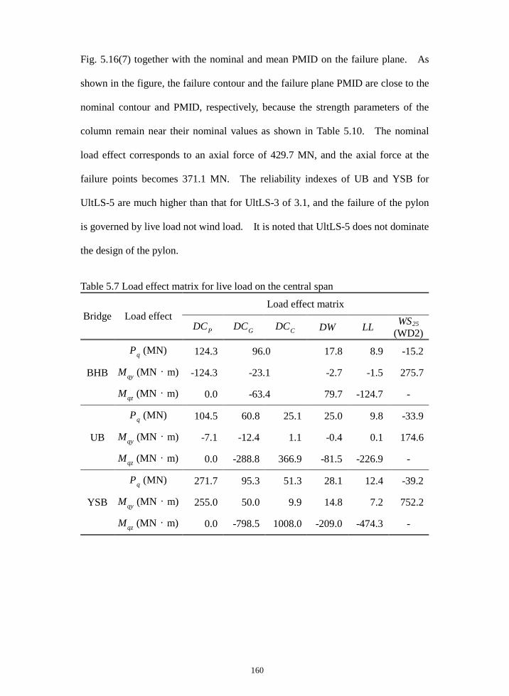
160

Fig. 5.16(7) together with the nominal and mean PMID on the failure plane. As

shown in the figure, the failure contour and the failure plane PMID are close to the

nominal contour and PMID, respectively, because the strength parameters of the

column remain near their nominal values as shown in Table 5.10. The nominal

load effect corresponds to an axial force of 429.7 MN, and the axial force at the

failure points becomes 371.1 MN. The reliability indexes of UB and YSB for

UltLS-5 are much higher than that for UltLS-3 of 3.1, and the failure of the pylon

is governed by live load not wind load. It is noted that UltLS-5 does not dominate

the design of the pylon.

Table 5.7 Load effect matrix for live load on the central span


DCP DCG DCC DW LL WS25 (WD2)

BHB

Pq (MN) 124.3 96.0 17.8 8.9 -15.2

Mqy (MN·m) -124.3 -23.1 -2.7 -1.5 275.7

Mqz (MN·m) 0.0 -63.4 79.7 -124.7 -

UB

Pq (MN) 104.5 60.8 25.1 25.0 9.8 -33.9

Mqy (MN·m) -7.1 -12.4 1.1 -0.4 0.1 174.6

Mqz (MN·m) 0.0 -288.8 366.9 -81.5 -226.9 -

YSB

Pq (MN) 271.7 95.3 51.3 28.1 12.4 -39.2

Mqy (MN·m) 255.0 50.0 9.9 14.8 7.2 752.2

Mqz (MN·m) 0.0 -798.5 1008.0 -209.0 -474.3 -

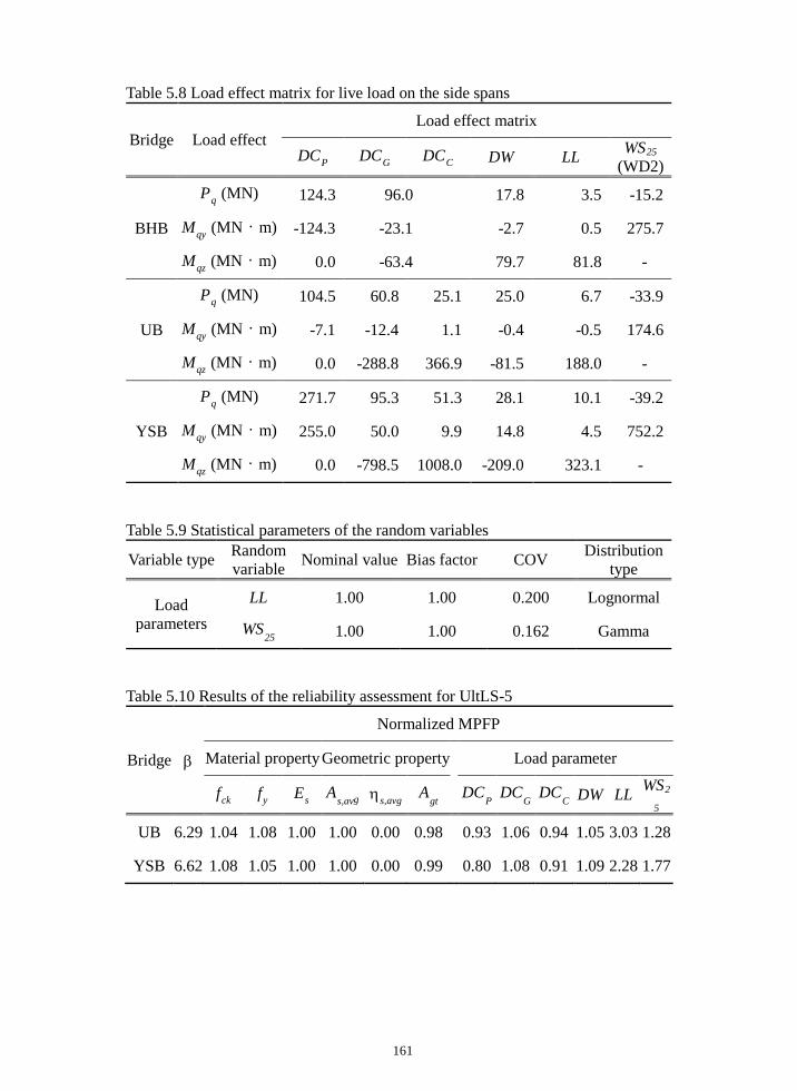
161

Table 5.8 Load effect matrix for live load on the side spans


DCP DCG DCC DW LL WS25 (WD2)

BHB

Pq (MN) 124.3 96.0 17.8 3.5 -15.2

Mqy (MN·m) -124.3 -23.1 -2.7 0.5 275.7

Mqz (MN·m) 0.0 -63.4 79.7 81.8 -

UB

Pq (MN) 104.5 60.8 25.1 25.0 6.7 -33.9

Mqy (MN·m) -7.1 -12.4 1.1 -0.4 -0.5 174.6

Mqz (MN·m) 0.0 -288.8 366.9 -81.5 188.0 -

YSB

Pq (MN) 271.7 95.3 51.3 28.1 10.1 -39.2

Mqy (MN·m) 255.0 50.0 9.9 14.8 4.5 752.2

Mqz (MN·m) 0.0 -798.5 1008.0 -209.0 323.1 -

Table 5.9 Statistical parameters of the random variables

Variable type Random variable Nominal value Bias factor COV Distribution

type

Load parameters

LL 1.00 1.00 0.200 Lognormal

WS25 1.00 1.00 0.162 Gamma

Table 5.10 Results of the reliability assessment for UltLS-5

Bridge β

Normalized MPFP


fck fy Es As,avg ηs,avg Agt DCP DCG DCC DW LL WS2

5

UB 6.29 1.04 1.08 1.00 1.00 0.00 0.98 0.93 1.06 0.94 1.05 3.03 1.28

YSB 6.62 1.08 1.05 1.00 1.00 0.00 0.99 0.80 1.08 0.91 1.09 2.28 1.77

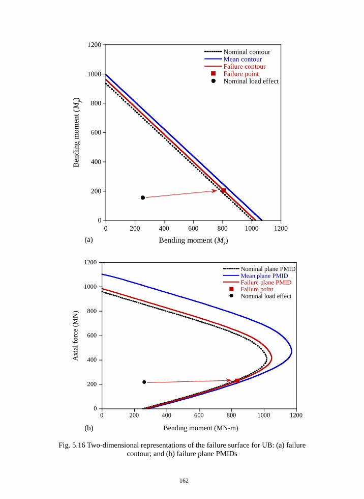
162

(a) (b)

Fig. 5.16 Two-dimensional representations of the failure surface for UB: (a) failure contour; and (b) failure plane PMIDs

0

200

400

600

800

1000

1200

0 200 400 600 800 1000 1200

Nominal contourMean contourFailure contourFailure pointNominal load effect

Ben

ding

mom

ent (

My)

Bending moment (Mz)

0

200

400

600

800

1000

1200

0 200 400 600 800 1000 1200

Nominal plane PMIDMean plane PMIDFailure plane PMIDFailure pointNominal load effect

Axi

al fo

rce

(MN

)


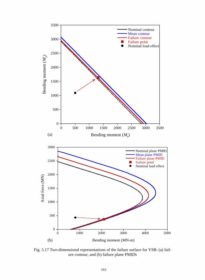
163

(a) (b)

Fig. 5.17 Two-dimensional representations of the failure surface for YSB: (a) fail-ure contour; and (b) failure plane PMIDs

0

500

1000

1500

2000

2500

3000

3500

0 500 1000 1500 2000 2500 3000 3500

Nominal contourMean contourFailure contourFailure pointNominal load effect

Ben

ding

mom

ent (

My)

Bending moment (Mz)

0

500

1000

1500

2000

2500

3000

0 1000 2000 3000 4000 5000

Nominal plane PMIDMean plane PMIDFailure plane PMIDFailure pointNominal load effect

Axi

al fo

rce

(MN

)


164

SECTION 6

CONCLUSIONS AND RECOMMENDATIONS FOR FURTHER STUDY

The equivalent static wind pressure, which is obtained by multiplying the gust fac-

tor to the static wind pressure induced by the mean wind velocity, is employed for

approximating the actual aerodynamic wind pressure. The probabilistic model of

wind velocity is established by using the annual maximum wind velocities meas-

ured at weather stations. A linear regression on the Gumbel probability paper is

applied to estimate the statistical parameters of wind velocity. To identify the re-

lationships between the statistical parameters of wind velocity and pressure, the

normalized wind pressure is defined by wind coefficients and velocity. The statis-

tical parameters of the normalized wind pressure are evaluated with Monte-Carlo

simulation, and the distribution type of the normalized wind pressure is confirmed

as through the Kolmogorov-Smirnov goodness-of-fit test. The mean, bias factor

and COV of the normalized wind velocity are approximated as linear functions of

the COV of wind velocity individually based on the results of Monte-Carlo simula-

tions. The derived relationships between the statistical parameter of wind velocity

and pressure are available for irrespective of the design life of a structure.

A new approach is proposed to estimate the reliability indexes of RC columns

subjected to uniaxial bending using the AFOSM without Monte-Carlo simulations.

The PMID of a column is taken as the limit state function. The material proper-

ties, the geometric properties, and the load parameters are considered as the ran-

dom variables. The HL-RF algorithm with gradient projection method is adopted

to solve the minimization problem defined in the AFOSM. The cubic spline in-

165

terpolation is utilized to form the explicit expression of the PMID. The sensitivi-

ties of the PMID are obtained through the direct differentiation of the PMID ap-

proximated by the cubic spline. The detailed sensitivity expressions of the axial

force and the bending moment with respect to the random variables are presented.

Since no assumption is made on the geometric shape of a cross-section in the cur-

rent formulation, the proposed scheme can be applicable to a variety of cross-

sections of RC columns. The proposed approach can be extended by adopting the

stress-strain relationship for the confinement and the strain hardening without any

modification if the statistical characteristics of the confined and hardening effects

on the strength of a column are available. The proposed reliability assessment

method is applied to pylon sections for five cable-supported bridges in Korea.

The limit state of a column is mainly governed by the load effect induced by the

wind load, while the strength parameters and dead loads have rather a minor effect

on the failure of columns.

A new robust methodology is proposed for determination of the load factors

and the design equation for a wind load-governed load combination, which are de-

rived by observing the characteristics of the MPFPs of the random variables for the

pylon sections of five cable-supported bridges in Korea. Based on the results of

the reliability analyses, the based load factors and design equation for WGLS are

proposed by using the geometric interpretation of a reliability index. The base

dead load factors are defined by the bias factors of the dead load components.

The analytical form of the base wind load factor, which is a function of the target

reliability and statistical parameters of the wind load, is derived. To demonstrate

the validity of the proposed load factors and design equation for RC columns, vali-

dation analyses are performed for the pylons of the five bridges. It is confirmed

166

that the pylon sections, determined by the proposed design equation and base load

factors corresponding to a specified target reliability index, secure the target relia-

bility for the five bridges within an acceptable error range regardless of the COV of

a wind load.

To adapt the base wind load factor to the several bridge design codes, an ad-

justment factor is introduced and is determined through a curve fitting approach.

The adjustment procedure of wind load factors is presented to utilize the dead load

factors and the resistance factor specified in AASHTO specifications, KHBDC

(LSD)-CB, and KHBDC (LSD). The adjusted wind load factor for the AASHTO

specifications is 1.42 that is very close to the wind load factor of 1.4 which is sug-

gested in the AASHTO specifications. It can be seen that the proposed load fac-

tors and adjustment procedure work very well. The adjusted wind load factor for

KHBDC (LSD)-CB is expressed as a function of the COV of wind velocity by us-

ing the relationships between statistical parameters of wind velocity and pressure.

The recurrence periods of the basic wind velocity for KHBDC (LSD)-CB are cal-

culated in order to yield target reliability indexes in conjunction with the wind load

factor of 1.0. The validity of the adjusted wind load factors for variations of a

cross-section is confirmed through the reliability assessment of RC pylons with

various sizes of cross-sections. Since the basic wind velocities currently present-

ed in KHBDC (LSD) does not secure a uniform reliability level, the proper basic

wind velocities are suggested to secure a target reliability index in case of the wind

load factor of 1.4 as specified in the design code.

The reliability indexes and MPFPs of RC columns under biaxial bending con-

ditions are calculated by combining the load contour method and the AFOSM.

The failure surface defined by the load contour method is utilized as the limit state

167

function, and constructed by the PMIDU for an RC column with respect to each

principal axis. The HL-RF algorithm with the gradient projection method is em-

ployed to solve the minimization problem of the AFOSM. The sensitivities of the

failure surface to the random variables are obtained by the direct differential meth-

od. The proposed approach is applied to estimate the reliability index of the RC

pylons subjected to biaxial bending. The variations of the reliability indexes for

the UltLS-3 with attack angles of the wind are investigated. The reliability level

for the UltLS-5 is assessed. The UltLS-5 does not seem to govern the designs of

pylons.

The proposed approach provides a very powerful tool for determining the

proper wind load factor for the along-wind direction in reliability-based specifica-

tions, and more aspects for extensions of the proposed method exist. Important

applications of the proposed method are discussed for three areas of further studies:

in evaluation of static and aerodynamic wind pressures, applications to steel col-

umns and surface exponent of biaxial bending.

Evaluation of static and aerodynamic wind pressures

In the evaluation of equivalent static wind pressure, the exposure coefficient

and gust factor are utilized to consider the wind environment of a bridge site and

the peak response due to the dynamic effect of wind, respectively. In most design

codes, the exposure coefficient is calculated using wind profile parameters based

on four terrain categories, which seems to be rather rough to take into account

complicated current wind environments in urban as well as rural areas. Therefore,

more detailed classification of the terrain category based on observed or simulated

wind profile may be preferable for the designs of wind-load governed long-span

168

bridges. The gust factors in KHBDC (LSD), Eurocode 2, and ASCE 7 are given as

functions of the dynamic characteristics of structures and turbulence intensity,

while KHBDC (LSD)-CB defines the gust factor in terms of the turbulence intensi-

ty only for heights less than 100m. As different gust factors appears in various

bridge design codes, their validity and accuracy should be investigated in a robust

way to draw more reasonable equivalent static wind pressure in bridge design.

This paper presents a general approach for evaluating wind load factor in the

along-wind direction using the equivalent static wind pressure without detailed

evaluation of aerodynamic wind pressure. In case the aerodynamic effect of wind

dominates dynamic behaviors of a structure, especially in the across-wind direction,

the aerodynamic wind pressure should be precisely evaluated using sophisticated

aerodynamic analysis. However, to include such an aerodynamic wind pressure

in an accurate sense for the code-calibration process, extensive further studies on

the statistical model of the aerodynamic wind pressure are required. Provided that

a proper statistical model of the aerodynamic effect of wind is reported and gener-

ally accepted among wind engineering societies in future, the proposed method can

be applied to calculate more realistic wind load factors.

Applications to Steel Columns

The base load factors proposed in this work are determined by considering on-

ly the statistical characteristics of the strength and load effect included in UltLS-3.

The base load factors should result in a desired target reliability index regardless of

material types of columns in case the statistical parameters of their strengths are

properly defined. Although the base load factors are tested only for RC columns

in this work, the proposed factors are believed to be applicable to steel columns as

169

the proposed approach depends upon the statistical characteristic of design varia-

bles rather than material type itself. Dissimilar to RC columns, however, the fail-

ure of a steel column may be caused by either material yielding or local/global

buckling depending on types of cross-sections, which are usually categorized into

compact and non-compact sections in girders. A great difficulty is expected in

modeling uncertainty of the strengths of steel columns especially when the buck-

ling strengths of steel columns govern failure because residual stresses, initial im-

perfections, etc affect the buckling strength of a steel column. Further extensive

researches on the statistical characteristics of the strengths of steel columns should

be performed through experimental as well as numerical studies. Once the proba-

bilistic descriptions of the strengths of steel columns are available, all the ap-

proaches presented in this study may be applicable to steel columns without modi-

fication to identify the wind load factor for steel columns

Surface exponents of biaxial bending

The reliability indexes of an RC column vary significantly with the surface ex-

ponent of the load contour, and thus most design codes set the surface exponent to

one for deducing conservative design. Although some studies on evaluation of

the surface exponent have been reported for rectangular columns, no study on sur-

face exponent for arbitrarily shaped sections such as hollowed sections has been

found so far. Further experimental and/or numerical studies are required to define

precise surface exponents of various shapes of cross-sections for more reasonable

design. If the precise surface exponent for a cross-section is specified, the pro-

posed scheme is applicable to any section type as no assumption is made on the

geometric shape of a cross-section in the current formulation.

170

REFERENCES

AASHTO (American Association of State Highway and Transportation Officials).

(2014). AASHTO LRFD Bridge Design Specifications, Washington, DC.

ACI (American Concrete Institute). (2001). ACI Design Handbook: Design of

structural reinforced concrete elements in accordance with the strength design

method of ACI 318-95, Farmington Hills, MI.

ACI (American Concrete Institute). (2011). Building Code Requirements for Rein-

forced Concrete (ACI 318-11) and Commentary, Farmington Hills, MI.

Ang, A. H-S., and Tang, W. H. (2007). Probability Concepts in Engineering: Em-

phasis on Applications in Civil and Environmental Engineering, 2nd ed., John

Wiley & Sons, Inc.

ASCE (American Society of Civil Engineers). (2013). “Minimum Design Loads

for Buildings and Other Structures” Standard ASCE/SEI 7-10, ASCE.

Bartlett, F. M., Hong, H. P., and Zhou, W. (2003). “Load factor calibration for the

proposed 2005 edition of the National Building Code of Canada: Statistics of

loads and load effects.” Canadian Journal of Civil Engineering, 30, 429-439.

Bonet, J. L., Miguel, P. F., Fernandez, M. A., and Romero, M. L. (2014). Analytical

Approach to Failure Surface in Reinforced Concrete Sections Subjected to Ax-

ial Loads and Biaxial Bending. Journal of Structural Engineering, ASCE,

130(12), 2006-2015.

Bresler, B. (1960). Design criteria for reinforced columns under axial load and bi-

axial bending. Journal Proceedings, ACI, 32(5), 481-490.

BSI (British Standard Institution). (2001). Steel, Concrete, and Composite Bridges

– Part 4: Code of practice for design of concrete bridges. BS 5400-4: 1990,

London.

171

CEN (Comité Européen de Normalization). (2010). “Actions on structures – Part 1-

4: General actions – Wind actions.” Eurocode 1, Brussels.

CEN (Comité Européen de Normalization). (2004). “Design of concrete structure –

Part 1-1: General rules and rules for buildings.” Eurocode 2, Brussels.

CSA (Canadian Standards Association). (2000). Canadian Highway Bridge Design

Code. CSA International.

Choi, Y. (2016). Formulation of P-M Interaction Diagram by Applying Uniformly

Distributed Reinforcement and Determination of RC Pylon Sections for Target

Reliability, Seoul National University. Master Thesis.

Conte, S. D., and der Boor, C. (1981). Elementary Numerical Analysis: An Algo-

rithmic Approach. 3th ed. McGraw-Hill.

Cunnane, C. (1978).” Unbiased plotting positions – a review.” Journal of Hydrolo-

gy, 37, 205-222.

Diniz, S. M. C., and Simiu E. (2005). “Probabilistic Descriptions of Wind Effects

and Wind-Load Factors for Database-Assisted Design.” Journal of Structural

Engineering, ASCE, 131(3), 507-516.

Ellingwood, B. (1977). Statistical analysis of RC beam-column interaction. Journal

of Structural Division, ASCE, ST7, 1377-1388.

Ellingwood, B. R., Galambos, T. V., MacGregor, J. G., and Cornell, C. A. (1980).

Development of a Probability Based Load Criterion for American National

Standard A58, Washington, DC: National Bureau of Standards.

Ellingwood, B. R., and Tekie, P. B. (1999). “Wind Load Statistics For Probability-

Based Structural Design.” Journal of Structural Engineering, ASCE, 125(4),

453-463.

Frangopol, D. M., Ide, Y., Spacone, E., and Iwaki, I. (1996). A new look at reliabil-

ity of reinforced concrete columns. Structural Safety, 18 (2/3), 123-150.

172

Gabbai, R. D., Fritz, W. P., Wright, A. P., and Simiu, E. (2008). “Assessment of

ASCE 7 Standard Wind Load Factors for Tall Building Response Estimates.”

Journal of Structural Engineering, ASCE, 134(5), 842-845.

Ghosn, M., Moses, F., and Wang, J. (2003). “Design of Highway Bridges for Ex-

treme Events.” NCHRP Report 489, Transportation Research Board, Washing-

ton, D.C.

Grant, L. H., Mirza, S. A., and MacGregor, J. G. (1978). Monte Carlo study of

strength of concrete columns. Journal Proceedings, ACI, 75, 348-358.

Gringorten, I. I. (1963). “A Plotting Rule for Extreme Probability Paper.” Journal

of Geophysical Research, 68(3), 813-814.

Haldar, A., and Mahadevan, S. (2000). Probability, Reliability and Statistical

Methods in Engineering Design, John Wiley & Sons, Inc., New York, 181-224.

Hassoun, M. N., and Al-Manaseer, A. (2012). Structural Concrete - Theory and

design, 5th ed. John Wiley and Sons, 389-406.

Hong, H. P., and Zhou, W. (1999). Reliability evaluation of RC columns. Journal

of Structural Engineering, ASCE, 125, 784-790.

Hong, H. P., Hu, Z., and King, J. P. C. (2009). “Gust response of bridges to spatial-

ly varying wind excitations and calibration of wind load factors.” HIIFP-075,

Highway Standards Branch, Ontario Ministry of Transportation.

Hsu, C-TT. (1986). Reinforced Concrete Members Subject to Combined Biaxial

Bending and Tension. Journal Proceedings, ACI, 83(1), 137-144.

Hsu, C-TT. (1988). Analysis and design of square and rectangular columns by

equation of failure surface. Structural Journal, ACI, 85(2), 167-179.

Jiang, Y., and Yang, W. (2013). An approach based on theorem of total probability

for reliability analysis of RC columns with random eccentricity. Structural

Safety, 41, 37-46.

173

JRA (Japan Road Association). (2007). Wind Resistant Design Manual for High-

way Bridge, Maruzen, Tokyo.

Kim, J. H., Lee, S. H., Paik, I., and Lee, H. S. (2015). “Reliability assessment of

reinforced concrete columns based on the P-M interaction diagram using

AFOSM.” Structural Safety, 55, 70-79.

Kim, J. H., and Lee, H. S. (2017). “Reliability assessment of reinforced concrete

rectangular columns subjected to biaxial bending using the load contour meth-

od.” Engineering Structures, 150, 636-645.

Kim, J. H., Yoo, C-H., and Lee, H. S. (2017). “Evaluation of wind load factors of

RC columns for wind load-governed limit stat in reliability-based design

code.” Journal of Bridge Engineering, ASCE, 22(9): 04017053.

Kim, S. (2018). Unified Code Calibration for Short- to Medium-span and Long-

span Bridges with New Vehicular Live Load Model, Seoul National University.

Master Thesis.

“Korea Meteorological Administration.” (2009). KMA, <https://web.kma.go.kr>

(Jan. 10, 2018).

KMOLIT (Korea Ministry of Land, Infrastructure and Transport). (2016a). Korean

Highway Bridge Design Code (Limit State Design), KMOLIT, Seoul.

KMOLIT (Korea Ministry of Land, Infrastructure and Transport). (2016b). Korean

Highway Bridge Design Code (Limit State Design) – Cable Supported Bridges,

KMOLIT, Seoul.

Kreyszig, E. (2006). Advanced Engineering Mathematics, 9th ed., John Wiley &

Sons, Inc.

KSCE (Korean Society of Civil Engineers). (2006). Design Guidelines for Cable

Supported Steel Bridges, KSCE, Seoul (Korean).

174

Lee, H. S., Kim, J. H., Lee, H. H., Lee, S. H., and Paik, I. (2016). “Korean High-

way Bridge Design Code (Limit State Design) – Cable Supported Bridges:

Code Calibration.”, KBRC TRS 048, Korea Bridge Design and Engineering Re-

search Center, Seoul (Korean).

Liu, P. L., and Der Kiureghian, A. (1991). Optimization algorithms for structural

reliability. Structural Safety, 9, 161-177.

McCormac, J. C., and Brwon, R. H. (2014). Design of Reinforced Concrete, 9th ed.

John Wiley and Sons, 302-316.

Milner, D. M., Spacone, E., and Frangopol, D. M. (2001). New light on perfor-

mance of short and slender reinforced concrete columns under random loads.

Engineering Structures, 23, 147-157.

Minciarelli, F., Gioffre M., Grigoriu M., and Simiu, E. (2001). “Estimates of ex-

treme wind effects and wind load factors: influence of knowledge uncertain-

ties.” Probabilistic Engineering Mechanics, 16, 331-340.

Mirza, S. A. (1996). Reliability-based design of reinforced concrete columns.

Structural Safety, 18 (2/3), 179-194.

Nilson, A. H., Darwin, D., and Dolan, C. W. (201). Design of Concrete Structures.

14th ed. McGraw-Hill.

Nowak, A. S., Yamani, A. S., and Tabsh, S. W. (1994). Probabilistic models for re-

sistance of concrete bridge girders. Structural Journal, ACI, 91 (3), 269-276.

Nowak, A. S. (1999). “Calibration of LRFD bridge design code.” NCHRP Report

368, Transportation Research Board, Washington, D.C.

Nowak, A. S., and Szerszen, M. M., (2003). Calibration of design code for build-

ings (ACI 318): Part 1-Statistical models for resistance. Structural Journal,

ACI, 100 (3), 377-382.

175

Nowak, A. S., and Eamon, C. D. (2008). Reliability analysis of plank decks. Jour-

nal of Bridge Engineering, ASCE, 13 (5), 540-546.

Pannell, F. N. (1963). Failure Surfaces for Members in Compression and Biaxial

Bending. Journal Proceedings, ACI, 60(1), 129- 140.

Parme, A. L., and Nieves, J. M. (1966). Capacity of Reinforced Rectangular Col-

umns Subject to Biaxial Bending. Journal Proceedings, ACI, 63(9), 911-923.

Rackwitz, R., and Fiessler, B. (1978). “Structural reliability under combined ran-

dom load sequences.” Computers & Structures, 9(5), 489-494.

Rogers, A. L., and Rogers, J. W., and Manwell, J. F. (2005). “Comparison of the

performance of four measure-correlate-predict algorithms.” Journal of Wind

Engineering Industrial Aerodynamics, 93, 243-264.

Simiu, E., and Scanlan, R. H. (1999). Wind Effects on Structures – Fundamentals

and Application to Design, John Wiley & Sons, Inc., New York, 327-331.

Stewart, M. G., and Attard, M. M. (1999). Reliability and model accuracy for high-

strength concrete column design. Journal of Structural Engineering, ASCE,

125, 290-300.

Szerszen, M. M., Szwed, A., and Nowak, A. S. (2005). Reliability analysis for ec-

centrically loaded columns. Structural Journal, ACI, 102 (5), 676-688.

Wang, C. K., and Salmon, C. G. (1992). Reinforced Concrete Design. 5th ed. Har-

per Collins, New York.

Wang, W., and Hong, H. P. (2002). Reliability of reinforced concrete columns un-

der axial load and biaxial bending. 4th Structural Specialty Conference of the

Canadian Society for Civil Engineering, 5(1), 1819-1827.

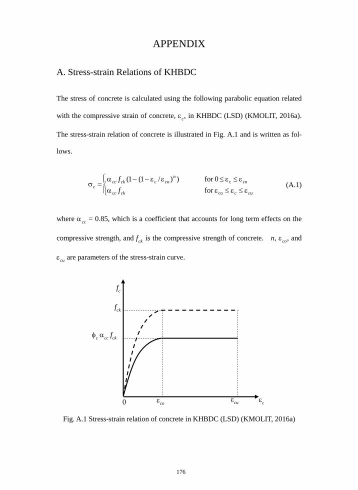
176

APPENDIX

A. Stress-strain Relations of KHBDC

The stress of concrete is calculated using the following parabolic equation related

with the compressive strain of concrete, εc, in KHBDC (LSD) (KMOLIT, 2016a).

The stress-strain relation of concrete is illustrated in Fig. A.1 and is written as fol-

lows.

ε≤ε≤εαε≤ε≤εε−−α

=σcucckcc

con

cocckccc f

f

co

c

for 0for ))/1(1(

(A.1)

where αcc = 0.85, which is a coefficient that accounts for long term effects on the

compressive strength, and fck is the compressive strength of concrete. n, εco, and

εcu are parameters of the stress-strain curve.

Fig. A.1 Stress-strain relation of concrete in KHBDC (LSD) (KMOLIT, 2016a)

fc

fck

φc αcc fck

εco εcu εc 0

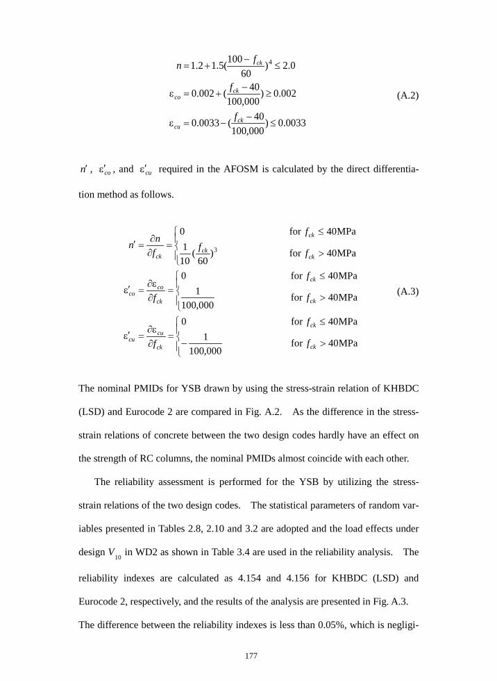
177

0033.0)000,100

40(0033.0

002.0)000,100

40(002.0

0.2)60

100(5.12.1 4

≤−

−=ε

≥−

+=ε

≤−

+=

ckcu

ckco

ck

f

f

fn

(A.2)

n′ , coε′ , and cuε′ required in the AFOSM is calculated by the direct differentia-

tion method as follows.

>−

≤=

∂ε∂

=ε′

>

≤=

∂ε∂

=ε′

>

≤=

∂∂

=′

MPa40for 000,100

1MPa40for 0

MPa40for 000,100

1MPa40for 0

MPa40for )60

(101

MPa40for 0

3

ck

ck

ck

cucu

ck

ck

ck

coco

ckck

ck

ck

f

f

f

f

f

f

fff

fnn

(A.3)

The nominal PMIDs for YSB drawn by using the stress-strain relation of KHBDC

(LSD) and Eurocode 2 are compared in Fig. A.2. As the difference in the stress-

strain relations of concrete between the two design codes hardly have an effect on

the strength of RC columns, the nominal PMIDs almost coincide with each other.

The reliability assessment is performed for the YSB by utilizing the stress-

strain relations of the two design codes. The statistical parameters of random var-

iables presented in Tables 2.8, 2.10 and 3.2 are adopted and the load effects under

design V10 in WD2 as shown in Table 3.4 are used in the reliability analysis. The

reliability indexes are calculated as 4.154 and 4.156 for KHBDC (LSD) and

Eurocode 2, respectively, and the results of the analysis are presented in Fig. A.3.

The difference between the reliability indexes is less than 0.05%, which is negligi-

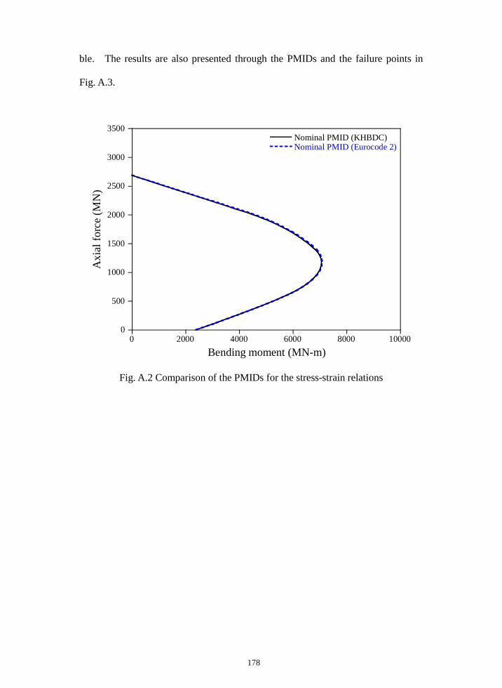
178

ble. The results are also presented through the PMIDs and the failure points in

Fig. A.3.

Fig. A.2 Comparison of the PMIDs for the stress-strain relations

0

500

1000

1500

2000

2500

3000

3500

0 2000 4000 6000 8000 10000

Nominal PMID (KHBDC)Nominal PMID (Eurocode 2)

Axi

al fo

rce

(MN

)


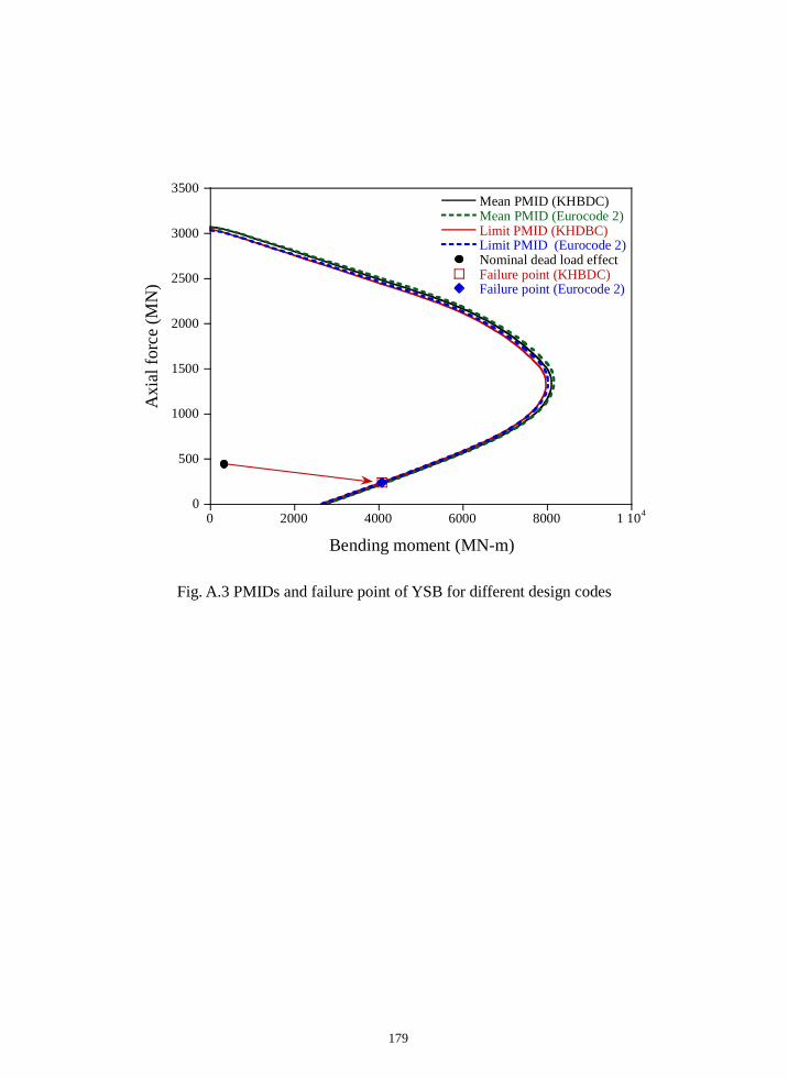
179

Fig. A.3 PMIDs and failure point of YSB for different design codes

0

500

1000

1500

2000

2500

3000

3500

0 2000 4000 6000 8000 1 104

Mean PMID (KHBDC)Mean PMID (Eurocode 2)Limit PMID (KHDBC)Limit PMID (Eurocode 2)Nominal dead load effectFailure point (KHBDC)Failure point (Eurocode 2)

Axi

al fo

rce

(MN

)


180

초 록

김지현

건설환경공학부

서울대학교 대학원

이 연구에서는 신뢰도기반 교량 설계기준의 풍하중지배조합에 대한 풍하

중계수를 풍하중의 통계적 특성을 기반으로 하여 결정하는 방법을 제안

하였다. 풍하중에 의해서 발생하는 공기역학적 풍압을 근사하기 위하여

거스트계수를 이용하여 등가의 적정풍압을 정의하였다. 측정된 풍속 데

이터를 기반으로 풍속 및 풍압의 확률모형을 정립하며, 몬테-카를로 모

사법을 이용하여 풍압의 확률모델을 구성 한 후 그 통계특성을 추정하였

다. 일반적인 교량 설계기준에서는 풍하중의 공칭값을 풍속으로 정의하

고 있기 때문에, 신뢰도기반 하중계수 결정을 위하여 풍속 및 풍압의 통

계특성간의 관계식을 확립하였다.

개선된일계이차모멘트법을 이용하여 철근콘크리트 기둥의 신뢰도해

석 기법을 각각 개발하였으며, 대한민국에서 공용되고 있는 5개 케이블

지지 교량의 철근콘크리트 주탑의 풍하중지배 조합에 대한 신뢰도해석을

수행하였다. 신뢰도평가를 위한 한계상태식은 철근콘크리트 기둥의 강도

를 나타내는 P-M 상관도를 이용하여 정의 되었으며, 하중 및 강도변수

를 확률변수로 고려하였다. 다섯 케이블지지 교량의 신뢰도해석 결과 풍

하중을 제외한 모든 확률변수가 평균에서 파괴하는 것을 확인 할 수 있

181

었다. 또한, 표준정규분포 공간 상에서 풍하중의 파괴점에 상응하는 비초

과확률이 계산된 신뢰도지수에 상응하는 파괴확률과 매우 근사한 값을

보였다. 따라서 신뢰도기반 하중저항계수의 이론적 정의에 따라 고정하

중계수는 각 고정하중의 편심계수로 정의하였으며, 평균값에 의하여 결

정되는 P-M 상관도를 이용하여 설계식을 정의하였다. 풍하중의 파괴점

은 주어진 목표신뢰도지수에 상응하는 파괴확률과 같은 비초과확률을 가

지는 표준정규분포 공간상에서의 점으로 가정하였으며, 검블분포 및 표

준 정규분포의 누적분포함수로부터 목표신뢰도지수를 확보하게 하는 풍

하중계수를 해석적인 함수로 표현하였다. 그 함수는 목표신뢰도지수 및

풍압의 통계 특성으로 표현되었다. 하중저항계수의 이론적 정의에 따라

계산된 하중계수를 기본 하중계수로 정의하였다. 기본 풍하중계수의 유

효성은 다섯 교량의 철근콘크리트 주탑의 신뢰도평가 결과로부터 확인하

였으며, 그 결과 제안된 풍하중계수가 오차범위 2%내로 매우 정확하게

목표신뢰도지수를 산정하도록 결정 된 것을 확인 할 수 있었다.

위와 같이 계산된 기본 풍하중계수는 고정하중계수가 모두 편심계수

로 정의되며 설계식이 저항의 평균값으로 구성될 때 성립하는 풍하중계

수이다. 따라서 각 설계기준에서 제시하는 고정하중 및 설계식에 적용하

기 위해서는 풍하중계수를 조정하는 조정 절차가 필요하다. 이 연구에서

는 국내외 여러 교량설계기준을 위하여 기본 풍하중계수를 조정하는 절

차를 제안하였다. 조정 절차를 AASHTO 교량 설계기준에 적용하여 조정

된 풍하중계수를 계산하였으며 그 값을 설계기준에 제시되어 있는 풍하

중계수와 비교함으로써 조정 절차의 타당성을 검증하였다. 도로교설계기

182

준(한계상태설계법)-케이블교량편을 위하여 기본 풍하중계수를 조정하였

으며, 설계기준의 기본풍속을 이용할 때 목표신뢰도지수를 만족하게 하

는 풍하중계수를 풍속의 변동계수에 대한 함수로 제시하였다. 또한 도로

교설계기준(한계상태설계법)-케이블교량편에 대하여 풍하중계수를 1로 가

정할 때 목표신뢰도수준을 만족하게 하는 기본풍속의 재현주기를 계산하

는 방법을 제시하였다. 다양한 강도 변화에 대한 풍하중계수의 유효성을

확인하기 위하여 단면의 크기를 조정하여 조정된 풍하중계수의 적용성을

검증 하였다. 도로교설계기준(한계상태설계법)의 지역별 기본풍속은 주어

진 풍하중계수 1.4에 대하여 목표신뢰도지수를 균일하게 확보하고 있지

않기 때문에, 목표신뢰도지수를 확보할 수 있는 기본풍속을 계산할 수

있는 해석적 표현식을 제시하였다.

풍하중이 단면의 주축 방향으로 작용하지 않거나, 풍하중 및 활하중

이 동시에 교량에 재하되는 경우에는 주탑 단면에 2축 휨이 발생한다.

이와 같이 2축휨을 받는 철근콘크리트 주탑의 신뢰도분석을 수행하였다.

풍하중이 단면에 작용하는 각도에 따른 신뢰도지수 변화를 분석하였으며,

풍하중 및 활하중이 동시에 재하 될 때 발생하는 하중조합에 대하여 신

뢰도분석을 수행하였다. 그 결과 풍하중 및 활하중이 동시에 재하되는

하중조합은 주탑의 설계를 지배 하지 않는 것을 확인 하였다.

주요어: 풍하중계수, 하중-저항계수결정, 파괴확률, 목표신뢰도지수, 철근

콘크리트기둥, 풍압, 신뢰도해석; 풍하중 통계; 이축 휨; 신뢰도기반 교량

설계기준

Documents

Ph.D. THESISstrana.snu.ac.kr/laboratory/theses/jhkim2018.pdf · 2018-03-05 · measured wind data for reinforced concrete columns. The equivalent static wind pressure is adopted to