PID Skogestad

7/27/2019 PID Skogestad

http://slidepdf.com/reader/full/pid-skogestad 1/9

Finn Haugen: PID Control 211

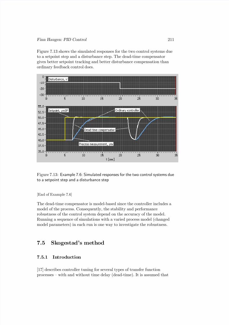
Figure 7.13 shows the simulated responses for the two control systems due

to a setpoint step and a disturbance step. The dead-time compensatorgives better setpoint tracking and better disturbance compensation thanordinary feedback control does.

Figure 7.13: Example 7.6: Simulated responses for the two control systems dueto a setpoint step and a disturbance step

[End of Example 7.6]

The dead-time compensator is model-based since the controller includes amodel of the process. Consequently, the stability and performancerobustness of the control system depend on the accuracy of the model.Running a sequence of simulations with a varied process model (changedmodel parameters) in each run is one way to investigate the robustness.

7.5 Skogestad’s method

7.5.1 Introduction

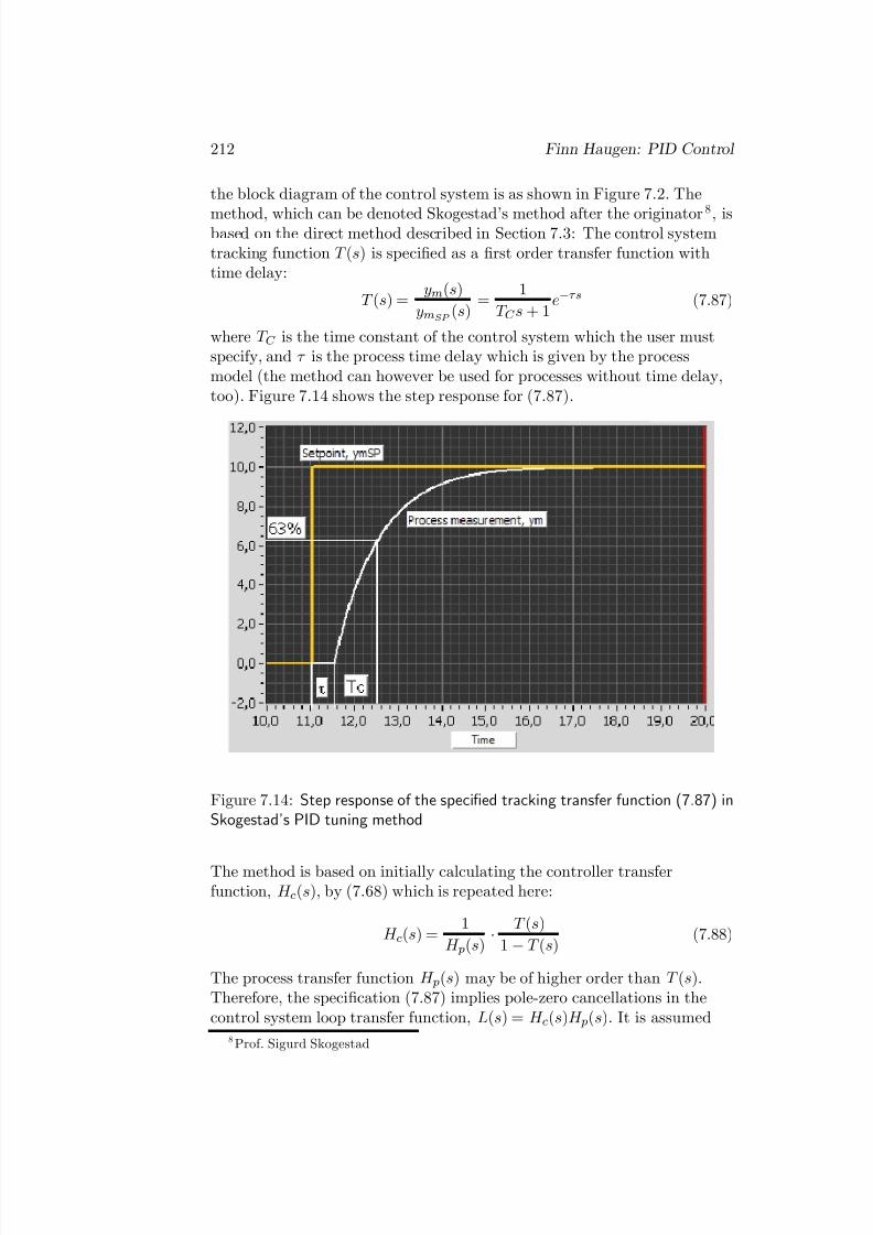
[17] describes controller tuning for several types of transfer functionprocesses — with and without time delay (dead-time). It is assumed that







214 Finn Haugen: PID Control

H p(s) (process) K p T i T dK s e−τ s 1

K (T C +τ ) k1 (T C + τ ) 0K

Ts+1e−τ s T

K (T C +τ ) min[T , k1 (T C + τ )] 0K

(Ts+1)se−τ s 1

K (T C +τ ) k1 (T C + τ ) T K

(T 1s+1)(T 2s+1)e−τ s T 1

K (T C +τ ) min[T 1, k1 (T C + τ )] T 2K s2e−τ s 1

4K (T C +τ )24 (T C + τ ) 4 (T C + τ )

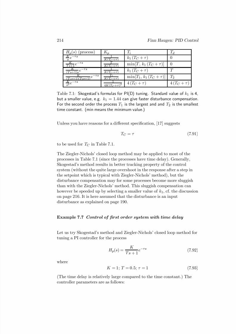
Table 7.1: Skogestad’s formulas for PI(D) tuning. Standard value of k1 is 4,but a smaller value, e.g. k1 = 1.44 can give faster disturbance compensation.For the second order the process T 1 is the largest and and T 2 is the smallesttime constant. (min means the minimum value.)

Unless you have reasons for a diff erent specification, [17] suggests

T C = τ (7.91)

to be used for T C in Table 7.1.

The Ziegler-Nichols’ closed loop method may be applied to most of theprocesses in Table 7.1 (since the processes have time delay). Generally,Skogestad’s method results in better tracking property of the controlsystem (without the quite large overshoot in the response after a step in

the setpoint which is typical with Ziegler-Nichols’ method), but thedisturbance compensation may for some processes become more sluggishthan with the Ziegler-Nichols’ method. This sluggish compensation canhowever be speeded up by selecting a smaller value of k1, cf. the discussionon page 216. It is here assumed that the disturbance is an inputdisturbance as explained on page 190.

Example 7.7 Control of fi rst order system with time delay

Let us try Skogestad’s method and Ziegler-Nichols’ closed loop method fortuning a PI controller for the process

H p(s) =K

Ts + 1e−τ s (7.92)

where

K = 1; T = 0.5; τ = 1 (7.93)

(The time delay is relatively large compared to the time constant.) Thecontroller parameters are as follows:




• Skogestad’s method, cf. Table 7.1 with (7.91) and k = 4:

K p = 0.25; T i = 0.5 (7.94)

• Ziegler-Nichols’ closed loop method:

K p = 0.68; T i = 2.43 (7.95)

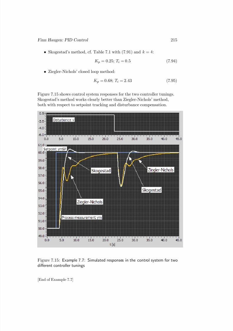
Figure 7.15 shows control system responses for the two controller tunings.Skogestad’s method works clearly better than Ziegler-Nichols’ method,both with respect to setpoint tracking and disturbance compensation.

Figure 7.15: Example 7.7: Simulated responses in the control system for twodiff erent controller tunings





7.5.3 Skogestad’s method with faster disturbance

compensation

According to [17], k1 is 4 in Table 7.1. However, through simulations Ihave observed that k1 = 4 in several cases gives quite sluggish disturbancecompensation, although the parameter formulas in Table 7.1 are developedto avoid unnecessary sluggish compensation. A reduced k1 value, ask1 = 1.44, can give considerably faster disturbance compensation (since theintegral time T i is reduced).11 A drawback of this modification of Skogestad’s method is that there will be somewhat larger overshoot in theresponse after setpoint step, but in most cases such an increased overshootis acceptable (if the setpoint is constant, which is typical, there is no

overshoot, of course). Another drawback of the modification is that thestability robustness of the loop is somewhat reduced because of thereduced T i.

Example 7.8 PI control of integrator with time delay

The process

H p(s) =K

se−τ s (7.96)

whereK = 1; τ = 0.5 (7.97)

will be controlled by a PI controller. (The wood-chip tank described inExample 2.3 has such a transfer function model.) Below are the PIparameters according to various tuning methods:

• Skogestad’s method, cf. Table 7.1, with (7.91) and k1 = 4:

K p = 1; T i = 4 (7.98)

• Skogestad’s method, cf. Table 7.1, with (7.91) and k1 = 1.44:

K p = 1; T i = 1.44 (7.99)

11 According to [17] the standard value k1 = 4 gives a transfer function from disturbancev to process measurement ym in the control system with characteristic polynomial as of a critically damped second order system, i.e. the relative damping factor is ζ = 1. Thisis quite a conservative choice. Faster but less damped dynamics is obtained with ζ < 1.Simulations shows that ζ = 0.6 is a reasonable value. It gives almost 3 times smaller T iand therefore faster disturbance compensation. ζ = 0.6 is obtained with k1 = 1.44. Itcan be shown that the phase margin, PM , of a loop having second order characteristicpolynomial is approximately equal to 100◦ · ζ . With ζ = 0.6 this equals 60◦ — a reasonablevalue in most cases.




• Ziegler-Nichols’ closed loop method:

K p = 1.3; T i = 1.78 (7.100)

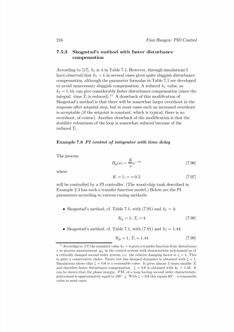
Figure 7.16 shows simulated responses in the control system for the threediff erent sets of PI parameter values. Skogestad’s method with k1 = 4seems to give the best set point tracking, but there are no oscillations,indicating good (too good?) stability. The disturbance compensation withSkogestad’s method with k1 = 4 is clearly the slowest of the threealternatives.

Figure 7.16: Example 7.8: Simulated responses in the control system for variousPI tunings


Example 7.7 demonstrated that it may be beneficial to set k1 = 1.44 instead of the standard value k1 = 4 because faster disturbance is then




obtained. Let us review Example 7.7 which demonstrated that k1 = 4 gave

fast and properly damped disturbance compensation. Since k1 = 4 workedwell in that example, will the disturbance compensation in that examplebe worse with k1 = 1.44 than with k1 = 4? The answer is no, because: K pis in any case independent of k1, so it has value 0.25. However, T i isdependent of k1. According to Table 7.1,T i = min [T , k1 (T C + τ )] = min [T , 2k1τ ], but this minimum value is 0.5no matter if k1 is 4 or 1.44. So, this example has indicated that even if k1 = 4 works fine, the suggestion k1 = 1.44 makes no harm in this case.

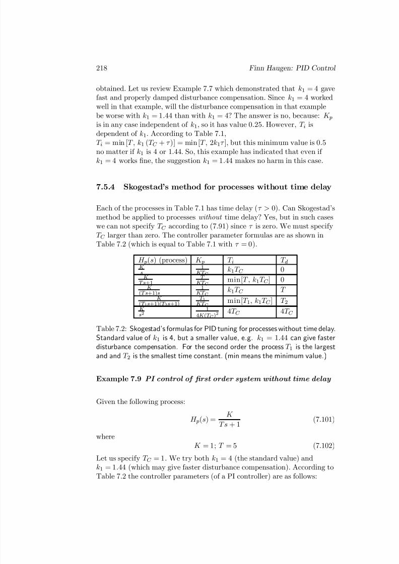
7.5.4 Skogestad’s method for processes without time delay

Each of the processes in Table 7.1 has time delay (τ > 0). Can Skogestad’smethod be applied to processes without time delay? Yes, but in such caseswe can not specify T C according to (7.91) since τ is zero. We must specifyT C larger than zero. The controller parameter formulas are as shown inTable 7.2 (which is equal to Table 7.1 with τ = 0).

H p(s) (process) K p T i T dK s

1KT C

k1T C 0K

Ts+1T

KT C min[T , k1T C ] 0

K (Ts+1)s

1KT C

k1T C T

K (T 1s+1)(T 2s+1)

T 1KT C

min[T 1, k1T C ] T 2K s2

14K (T C )

2 4T C 4T C

Table 7.2: Skogestad’s formulas for PID tuning for processes without time delay.Standard value of k1 is 4, but a smaller value, e.g. k1 = 1.44 can give fasterdisturbance compensation. For the second order the process T 1 is the largestand and T 2 is the smallest time constant. (min means the minimum value.)

Example 7.9 PI control of fi rst order system without time delay

Given the following process:

H p(s) =K

Ts + 1(7.101)

whereK = 1; T = 5 (7.102)

Let us specify T C = 1. We try both k1 = 4 (the standard value) andk1 = 1.44 (which may give faster disturbance compensation). According toTable 7.2 the controller parameters (of a PI controller) are as follows:




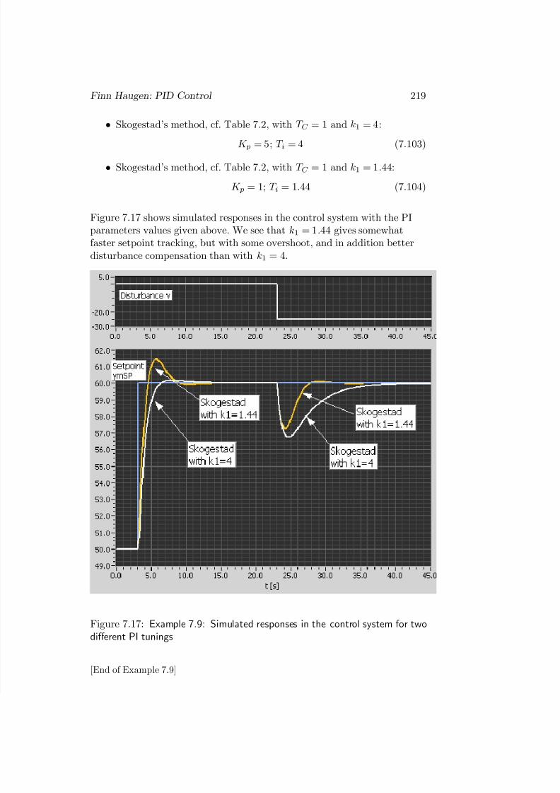
• Skogestad’s method, cf. Table 7.2, with T C = 1 and k1 = 4:

K p = 5; T i = 4 (7.103)

• Skogestad’s method, cf. Table 7.2, with T C = 1 and k1 = 1.44:

K p = 1; T i = 1.44 (7.104)

Figure 7.17 shows simulated responses in the control system with the PIparameters values given above. We see that k1 = 1.44 gives somewhatfaster setpoint tracking, but with some overshoot, and in addition betterdisturbance compensation than with k1 = 4.

Figure 7.17: Example 7.9: Simulated responses in the control system for twodiff erent PI tunings


Documents

PID Skogestad