Primer on Simulink Verson 1.0 (September 2004) Dr. Frank Kelso (UMN)

1.0 Introduction The behavior of dynamic systems can be modeled using differential equations. Simulink

is the software tool we will use for solving these differential equations. Because Simulink

shares the Matlab workspace, we will also use Matlab to parameterize the Simulink

model and plot the solution.

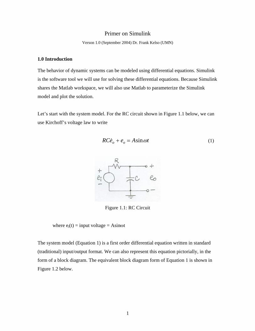
Let’s start with the system model. For the RC circuit shown in Figure 1.1 below, we can

use Kirchoff’s voltage law to write

tAeeRC oo ωsin=+& (1)

Figure 1.1: RC Circuit

where ei(t) = input voltage = Asinωt

The system model (Equation 1) is a first order differential equation written in standard

(traditional) input/output format. We can also represent this equation pictorially, in the

form of a block diagram. The equivalent block diagram form of Equation 1 is shown in

Figure 1.2 below.

1

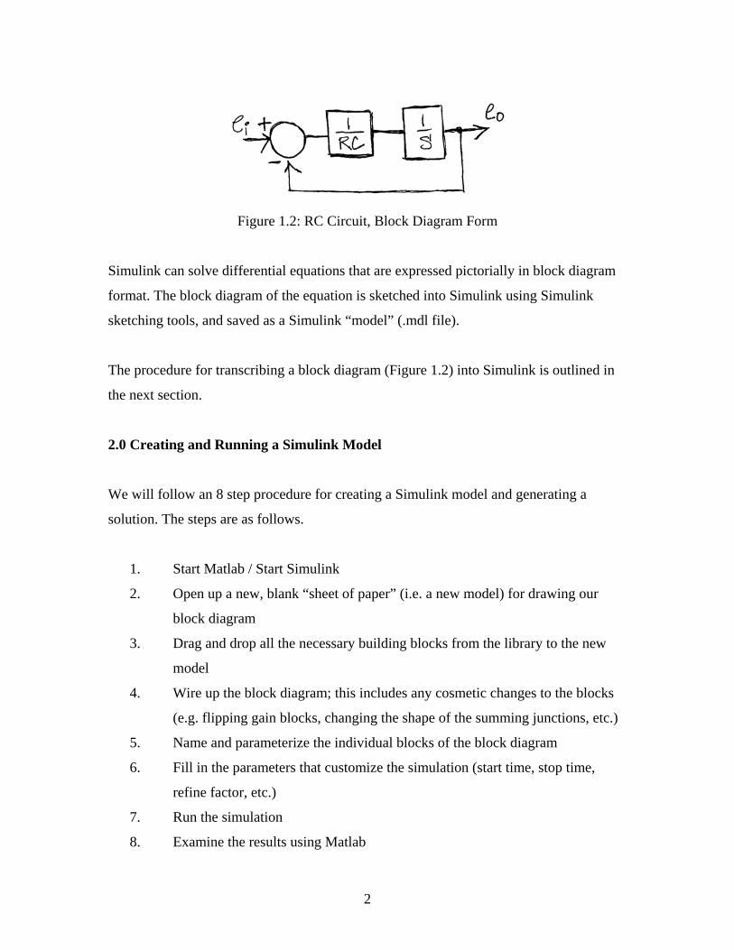
Figure 1.2: RC Circuit, Block Diagram Form

Simulink can solve differential equations that are expressed pictorially in block diagram

format. The block diagram of the equation is sketched into Simulink using Simulink

sketching tools, and saved as a Simulink “model” (.mdl file).

The procedure for transcribing a block diagram (Figure 1.2) into Simulink is outlined in

the next section.

2.0 Creating and Running a Simulink Model

We will follow an 8 step procedure for creating a Simulink model and generating a

solution. The steps are as follows.

1. Start Matlab / Start Simulink

2. Open up a new, blank “sheet of paper” (i.e. a new model) for drawing our

block diagram

3. Drag and drop all the necessary building blocks from the library to the new

model

4. Wire up the block diagram; this includes any cosmetic changes to the blocks

(e.g. flipping gain blocks, changing the shape of the summing junctions, etc.)

5. Name and parameterize the individual blocks of the block diagram

6. Fill in the parameters that customize the simulation (start time, stop time,

refine factor, etc.)

7. Run the simulation

8. Examine the results using Matlab

2

Step 1: Start Matlab / Start Simulink

On a Windows machine, begin by going to the “Start” menu and starting up Matlab

(usually found under “Programs”). Simulink uses the Matlab “engine” to solve equations,

and so Matlab needs to be run first.

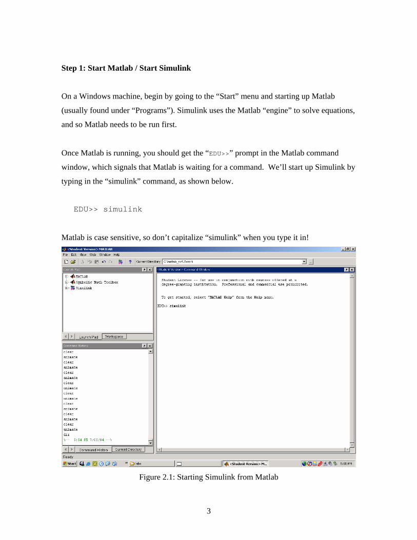
Once Matlab is running, you should get the “EDU>>” prompt in the Matlab command

window, which signals that Matlab is waiting for a command. We’ll start up Simulink by

typing in the “simulink” command, as shown below.

EDU>> simulink

Matlab is case sensitive, so don’t capitalize “simulink” when you type it in!

Figure 2.1: Starting Simulink from Matlab

3

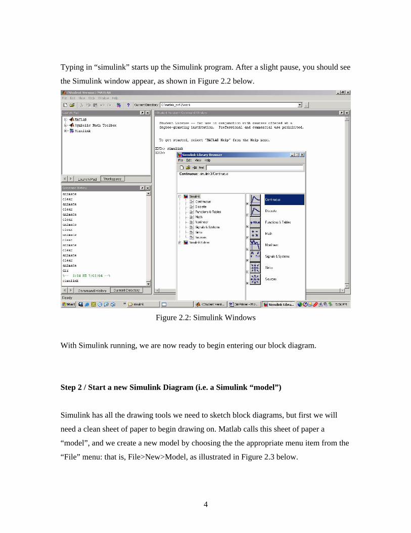
Typing in “simulink” starts up the Simulink program. After a slight pause, you should see

the Simulink window appear, as shown in Figure 2.2 below.

Figure 2.2: Simulink Windows

With Simulink running, we are now ready to begin entering our block diagram.

Step 2 / Start a new Simulink Diagram (i.e. a Simulink “model”)

Simulink has all the drawing tools we need to sketch block diagrams, but first we will

need a clean sheet of paper to begin drawing on. Matlab calls this sheet of paper a

“model”, and we create a new model by choosing the the appropriate menu item from the

“File” menu: that is, File>New>Model, as illustrated in Figure 2.3 below.

4

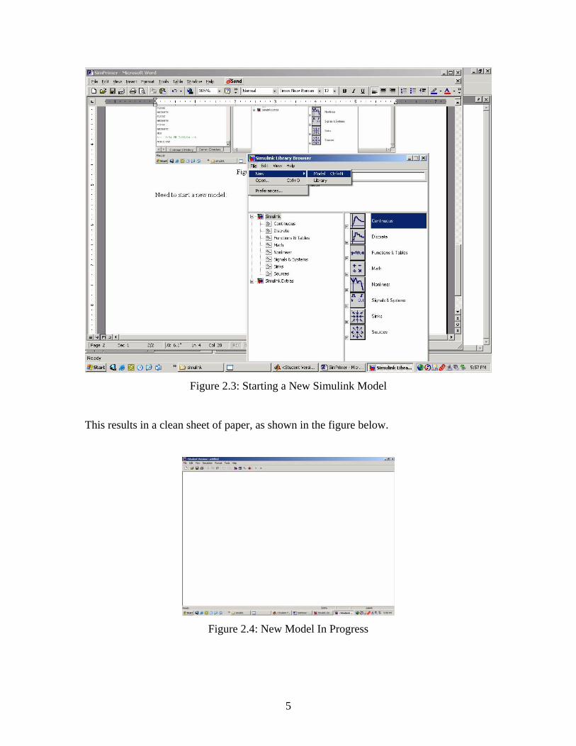
Figure 2.3: Starting a New Simulink Model

This results in a clean sheet of paper, as shown in the figure below.

Figure 2.4: New Model In Progress

5

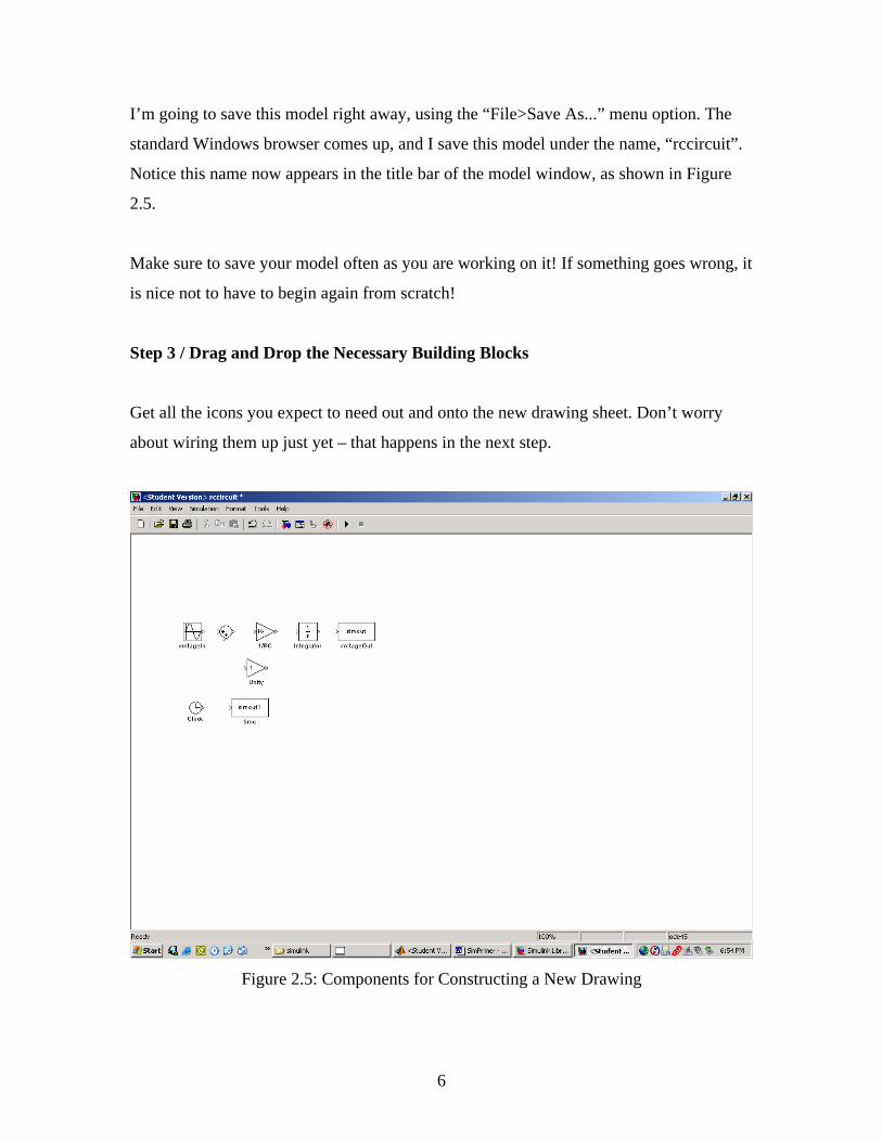
I’m going to save this model right away, using the “File>Save As...” menu option. The

standard Windows browser comes up, and I save this model under the name, “rccircuit”.

Notice this name now appears in the title bar of the model window, as shown in Figure

2.5.

Make sure to save your model often as you are working on it! If something goes wrong, it

is nice not to have to begin again from scratch!

Step 3 / Drag and Drop the Necessary Building Blocks

Get all the icons you expect to need out and onto the new drawing sheet. Don’t worry

about wiring them up just yet – that happens in the next step.

Figure 2.5: Components for Constructing a New Drawing

6

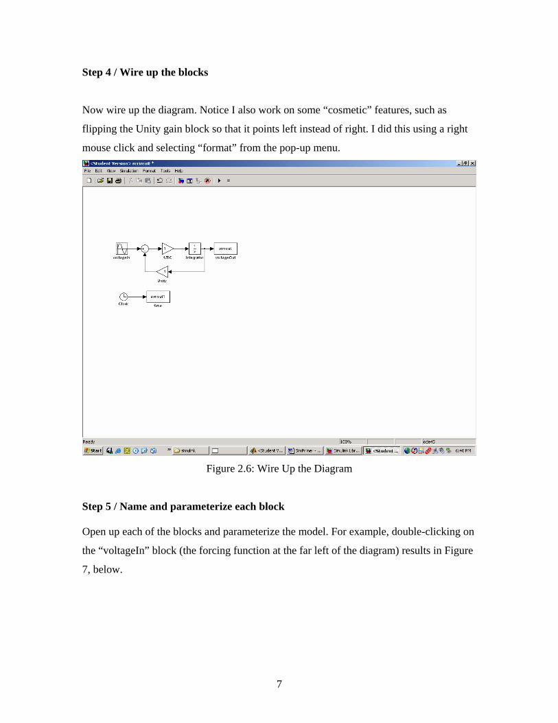
Step 4 / Wire up the blocks

Now wire up the diagram. Notice I also work on some “cosmetic” features, such as

flipping the Unity gain block so that it points left instead of right. I did this using a right

mouse click and selecting “format” from the pop-up menu.

Figure 2.6: Wire Up the Diagram

Step 5 / Name and parameterize each block Open up each of the blocks and parameterize the model. For example, double-clicking on

the “voltageIn” block (the forcing function at the far left of the diagram) results in Figure

7, below.

7

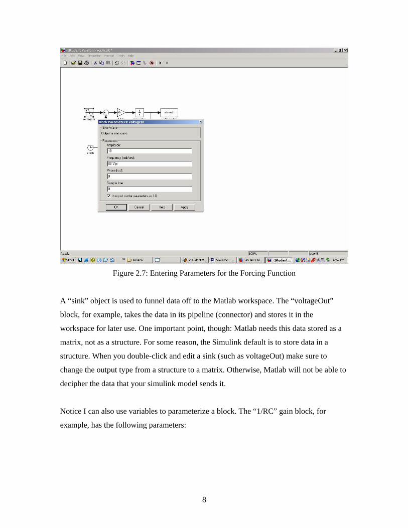
Figure 2.7: Entering Parameters for the Forcing Function

A “sink” object is used to funnel data off to the Matlab workspace. The “voltageOut”

block, for example, takes the data in its pipeline (connector) and stores it in the

workspace for later use. One important point, though: Matlab needs this data stored as a

matrix, not as a structure. For some reason, the Simulink default is to store data in a

structure. When you double-click and edit a sink (such as voltageOut) make sure to

change the output type from a structure to a matrix. Otherwise, Matlab will not be able to

decipher the data that your simulink model sends it.

Notice I can also use variables to parameterize a block. The “1/RC” gain block, for

example, has the following parameters:

8

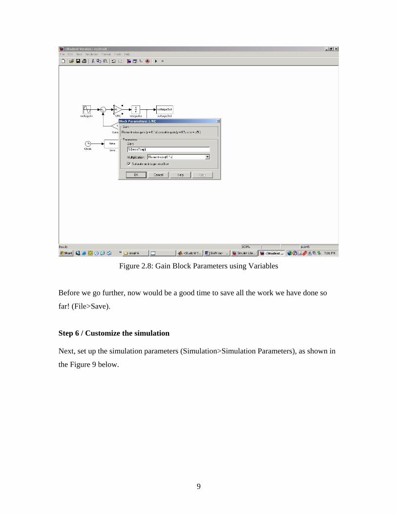
Figure 2.8: Gain Block Parameters using Variables

Before we go further, now would be a good time to save all the work we have done so

far! (File>Save).

Step 6 / Customize the simulation Next, set up the simulation parameters (Simulation>Simulation Parameters), as shown in

the Figure 9 below.

9

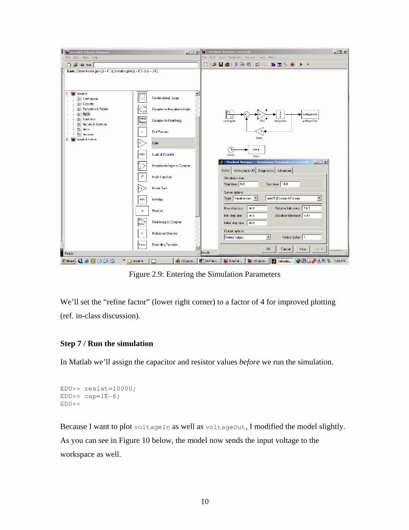
Figure 2.9: Entering the Simulation Parameters

We’ll set the “refine factor” (lower right corner) to a factor of 4 for improved plotting

(ref. in-class discussion).

Step 7 / Run the simulation In Matlab we’ll assign the capacitor and resistor values before we run the simulation.

EDU>> resist=10000; EDU>> cap=1E-6; EDU>>

Because I want to plot voltageIn as well as voltageOut, I modified the model slightly.

As you can see in Figure 10 below, the model now sends the input voltage to the

workspace as well.

10

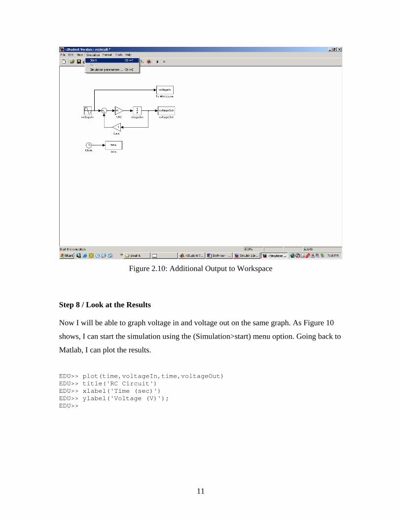
Figure 2.10: Additional Output to Workspace

Step 8 / Look at the Results Now I will be able to graph voltage in and voltage out on the same graph. As Figure 10

shows, I can start the simulation using the (Simulation>start) menu option. Going back to

Matlab, I can plot the results.

EDU>> plot(time,voltageIn,time,voltageOut) EDU>> title('RC Circuit') EDU>> xlabel('Time (sec)') EDU>> ylabel('Voltage (V)'); EDU>>

11

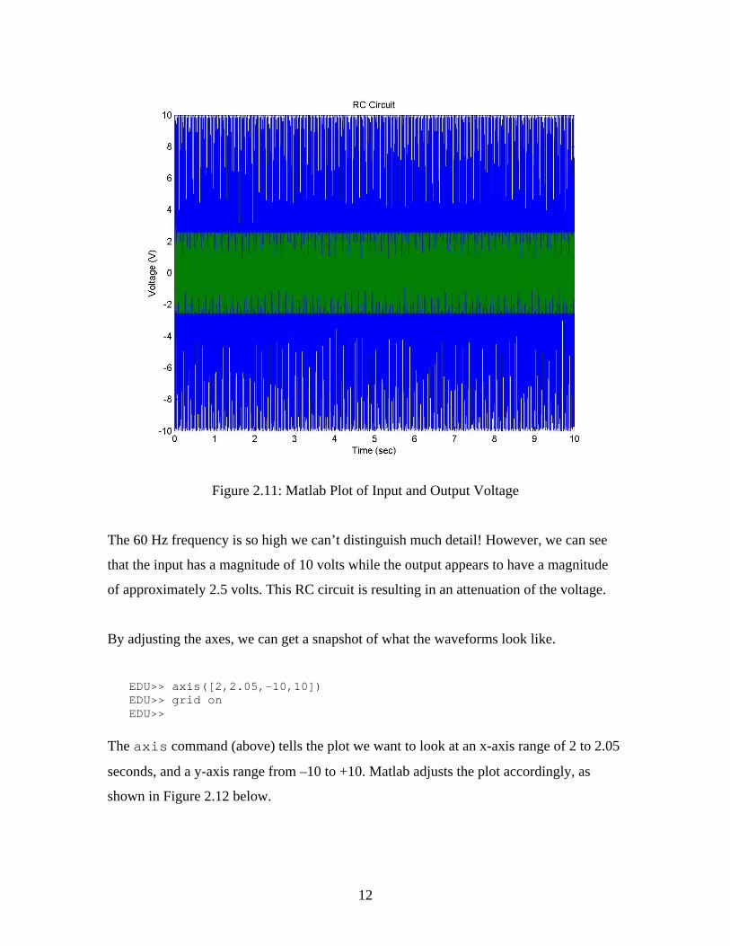
Figure 2.11: Matlab Plot of Input and Output Voltage

The 60 Hz frequency is so high we can’t distinguish much detail! However, we can see

that the input has a magnitude of 10 volts while the output appears to have a magnitude

of approximately 2.5 volts. This RC circuit is resulting in an attenuation of the voltage.

By adjusting the axes, we can get a snapshot of what the waveforms look like.

EDU>> axis([2,2.05,-10,10]) EDU>> grid on EDU>>

The axis command (above) tells the plot we want to look at an x-axis range of 2 to 2.05

seconds, and a y-axis range from –10 to +10. Matlab adjusts the plot accordingly, as

shown in Figure 2.12 below.

12

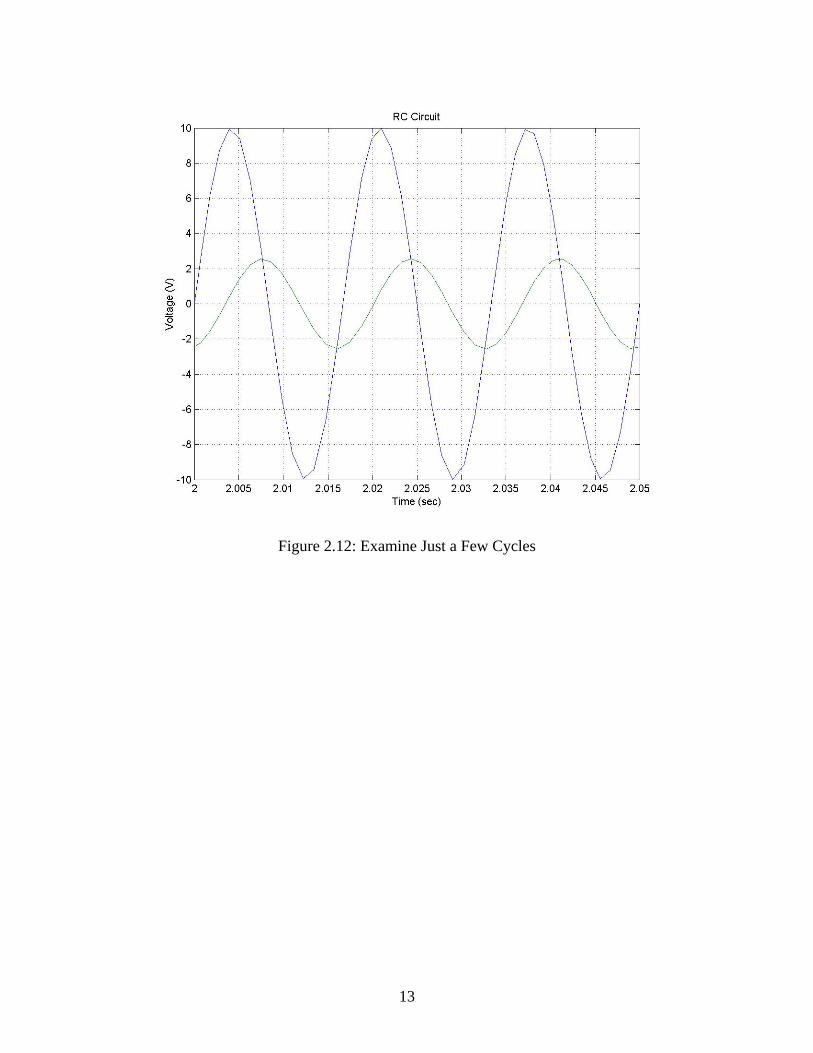
Figure 2.12: Examine Just a Few Cycles

13