Prof. Lecture 21: Electrostatic versus Electromagnetic

16.522, Space Propulsion Lecture 21 Prof. Manuel Martinez-Sanchez Page 1 of 21

16.522, Space Propulsion Prof. Manuel Martinez-Sanchez

Lecture 21: Electrostatic versus Electromagnetic Thrusters

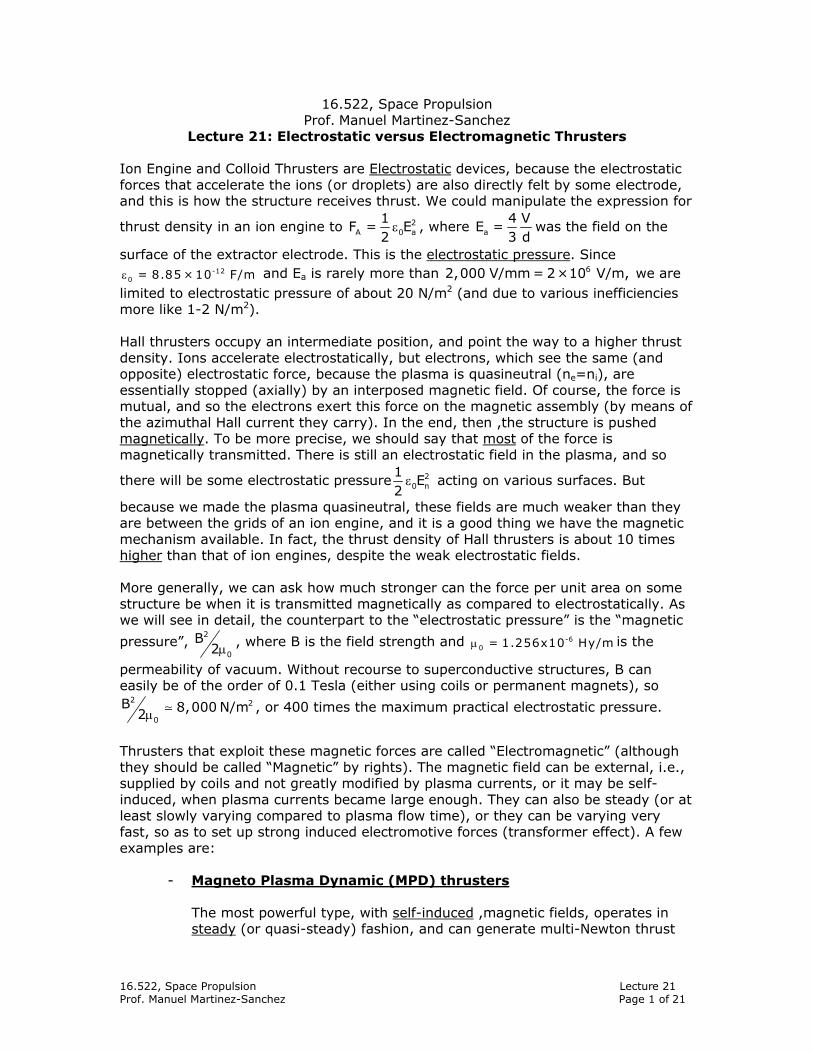
Ion Engine and Colloid Thrusters are Electrostatic devices, because the electrostatic forces that accelerate the ions (or droplets) are also directly felt by some electrode, and this is how the structure receives thrust. We could manipulate the expression for

thrust density in an ion engine to 2A 0 a

1F = E

2ε , where a

4 VE =

3 dwas the field on the

surface of the extractor electrode. This is the electrostatic pressure. Since -12

0 = 8.85 × 10 F/mε and Ea is rarely more than 62,000 V/mm = 2 ×10 V/m, we are limited to electrostatic pressure of about 20 N/m2 (and due to various inefficiencies more like 1-2 N/m2).

Hall thrusters occupy an intermediate position, and point the way to a higher thrust density. Ions accelerate electrostatically, but electrons, which see the same (and opposite) electrostatic force, because the plasma is quasineutral (ne=ni), are essentially stopped (axially) by an interposed magnetic field. Of course, the force is mutual, and so the electrons exert this force on the magnetic assembly (by means of the azimuthal Hall current they carry). In the end, then ,the structure is pushed magnetically. To be more precise, we should say that most of the force is magnetically transmitted. There is still an electrostatic field in the plasma, and so

there will be some electrostatic pressure 20 n

1E

2ε acting on various surfaces. But

because we made the plasma quasineutral, these fields are much weaker than they are between the grids of an ion engine, and it is a good thing we have the magnetic mechanism available. In fact, the thrust density of Hall thrusters is about 10 times higher than that of ion engines, despite the weak electrostatic fields. More generally, we can ask how much stronger can the force per unit area on some structure be when it is transmitted magnetically as compared to electrostatically. As we will see in detail, the counterpart to the “electrostatic pressure” is the “magnetic

pressure”, 2

0

B2µ , where B is the field strength and -6

0 = 1.256x10 Hy/mµ is the

permeability of vacuum. Without recourse to superconductive structures, B can easily be of the order of 0.1 Tesla (either using coils or permanent magnets), so

2 2

0

B 8,000 N/m2µ , or 400 times the maximum practical electrostatic pressure.

Thrusters that exploit these magnetic forces are called “Electromagnetic” (although they should be called “Magnetic” by rights). The magnetic field can be external, i.e., supplied by coils and not greatly modified by plasma currents, or it may be self-induced, when plasma currents became large enough. They can also be steady (or at least slowly varying compared to plasma flow time), or they can be varying very fast, so as to set up strong induced electromotive forces (transformer effect). A few examples are:

- Magneto Plasma Dynamic (MPD) thrusters

The most powerful type, with self-induced ,magnetic fields, operates in steady (or quasi-steady) fashion, and can generate multi-Newton thrust


levels with a few cm. diameter (compared to about 0.1 N for a 30 cm ion engine, or for a 10 cm Hall thruster).

- Applied field MPD thrusters

Here currents are less strong, so the main part of the B field is external. Still steady or quasi-steady.

- Pulsed Plasma Thrusters (PPT)

Pulsed Plasma Thrusters (PPT) are very similar in principle to self-field MPD, but they use a solid propellant (Teflon) which is ablated during each pulse of operation. These pulses last 10-20 sµ∼ only, but are just long

enough that induced emf fields (fromB

= ×Et

∂∇

∂) are still weak. Because

of various practical (mostly thermal) issues, PPT thrusters are not very

efficient <10%⎛ ⎞⎜ ⎟⎝ ⎠∼

, but they are simple and robust.

- Pulsed Inductive Thrusters (PIT)

Here the emphasis is on very fast magnetic risetime ( 1 -10 sµ∼ ) and the induced emf is used to break down the gas, ionize it, and drive a closed current loop that exerts the desired magnetic force. They can be thought of as a one-turn transformer in which the secondary is a plasma ring; the repulsion between primary and secondary accelerates the plasma away and pushes the primary coil forward. To avoid dissipating most of the

power in Ohmic losses, the device must be fairly large >0.5m⎛ ⎞⎜ ⎟⎝ ⎠∼

and

powerful (MW to GW of instantaneous power). In the following few lectures we will have time only to explore the self-field MPD type. We begin with some basic Physics.

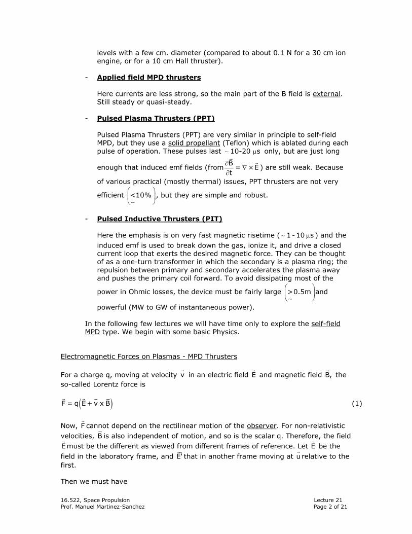
Electromagnetic Forces on Plasmas - MPD Thrusters For a charge q, moving at velocity v in an electric field E and magnetic field B, the so-called Lorentz force is

( )F = q E+ v x B (1)

Now, F cannot depend on the rectilinear motion of the observer. For non-relativistic velocities, B is also independent of motion, and so is the scalar q. Therefore, the field Emust be the different as viewed from different frames of reference. Let E be the

field in the laboratory frame, and E' that in another frame moving at u relative to the first. Then we must have


( )E+ v x B = E'+ v - u x B

so that

E' = E+u x B (2) (in particular, for u = v the Lorentz force is seen to be purely electrostatic; i.e.,

F = qE' ). Most often the frame at u is chosen to be that moving at the mean mass velocity of the plasma. Consider a plasma where there is a number density nj of the jth type of charged particle, which has a charge qj and moves at mean velocity jv . The net Lorentz force per unit volume is

( )jj jj

f = n q E+ v x B∑ (3)

and since the plasma is neutral j j

j

n q = 0∑ :

jj jj

f = n q v x B⎛ ⎞⎜ ⎟⎝ ⎠∑ (4)

But, by definition,

jj jj

n q v = j∑ (5)

where j is the current density vector (A/m2). So, finally, f = j x B (N/m3) (6) Notice that jv in Equation (5) could be in any frame, including the plasma frame. Ohm’s Law In most cases, the dominant contribution to j (Equation (5)) is from electrons, given their high mobility. In the plasma frame,

ee ej j = -en v (7) Notice that ev is the electron mean velocity vector, not to be confused with the mean thermal speed ec . The picture of electron motions is that of a very rapid, chaotic swarming of electrons back and forth (“going nowhere”), except that the whole swarm “slowly” drifts at ev .


Typically

e ev << c .

Let us make a crude model of the motion of the electron swarm. The net force on it per unit volume is

( )e e ef = -e E'+ v x B n (8)

where E' is used , since we are in the plasma frame. In steady state, this is balanced by the drag force opposing motion of electrons relative to the rest of the fluid, which we are assuming to be at rest, and whose particles have, by comparison, only a very slow thermal motion. To evaluate this drag, let eν be the effective collision frequency per electron for momentum transfer. This frequency is defined such that in each collision with a particle of “the rest of the fluid,” the electron is, on average, scattered by 90 , so that its forward momentum is completely lost. Then the mean drag force per unit volume is

e ee ee e e

mf = -n m v = j

eν

ν (9)

Equating the sum of (8) and (9) to zero,

( )2

ee

e e

e nj = E'+ v B

m ν×

or, since

e

e

jv = -

en,

2

e

e e e e

e n ej = E' - j × B

m mν ν

Define the scalar conductivity

2e

e e

e n=

mσ

ν (10)

and the Hall parameter

e e

eB B= ; =

m B

⎛ ⎞β β β ⎜ ⎟⎜ ⎟ν ⎝ ⎠

(11)

and we can write the generalized Ohm’s law as


E' = j+ j × σ β (12)

where, as given in Equation (2), E' = E+u x B . Remembering that the gyro frequency (the angular frequency of motion of an

electron orbiting about a perpendicular magnetic field B ) is e

eB= mω ,

e

=ω

βν

(13)

i.e. , it represents the ratio of gyro frequency to collision frequency; it can be expected to be high at low pressures and densities, where collisions are rare, and also at high magnetic field, where the gyro frequency is high. In many plasmas of interest in MHD or MPD, 1β ∼ . Electromagnetic Work The rate at which the external fields do work on the charged particles can be calculated (per unit volume) as

( )j jj jj

W = qn E+ v × B . v∑

jj jj

= E . qn v∑

or

W = E . j (14)

where we used ( )j jv × B . v 0≡ . We see here that the magnetic field does not

directly contribute to the total work, since the magnetic force is orthogonal to the particle velocity; it does, however, modify Eor j (depending on boundary conditions), and through them it does affect W. This total work goes partly into heating the plasma (dissipation) and partly into bodily pushing it (mechanical work). To see this, notice that

( ) ( )W = E . j = E' - u × B . j = E' . j+ j × B . u

(using ( ) ( )u × B . j = - j × B . u).

Also, using Ohm’s law

( )21 j

E' . j = j+ j × . j = βσ σ

where we used ( )j × . j = 0β .


Thus

( )2j

W = + j × B . uσ

(15)

The second term of this expression is simply the rate at which the Lorentz force j × B does mechanical work on the plasma moving at u . The first term is always positive and is the familiar Joule heating (also called Ohmic heating) effect. Notice how the presence of the magnetic field introduces the possibility of accelerating a plasma, in addition to the unavoidable heating. In an efficient accelerator, we would

try to maximize ( )j × B . u at the expense of 2j σ .

Origin of the magnetic field The magnetic field can either be provided by external coils, or induced directly by the

currents circulating in the plasma. The general relationship between B and j (in steady state and without magnetic materials) is Ampere’s law

0

Bj = × ∇

µ (16)

where -70 = 4 ×10µ π (in MKS units) is the permeability of vacuum.

In integral form

0

Bj . dA = .dl

µ∫∫ ∫ (17)

which states that the circulation of 0

Bµ

around a closed line equals the total current

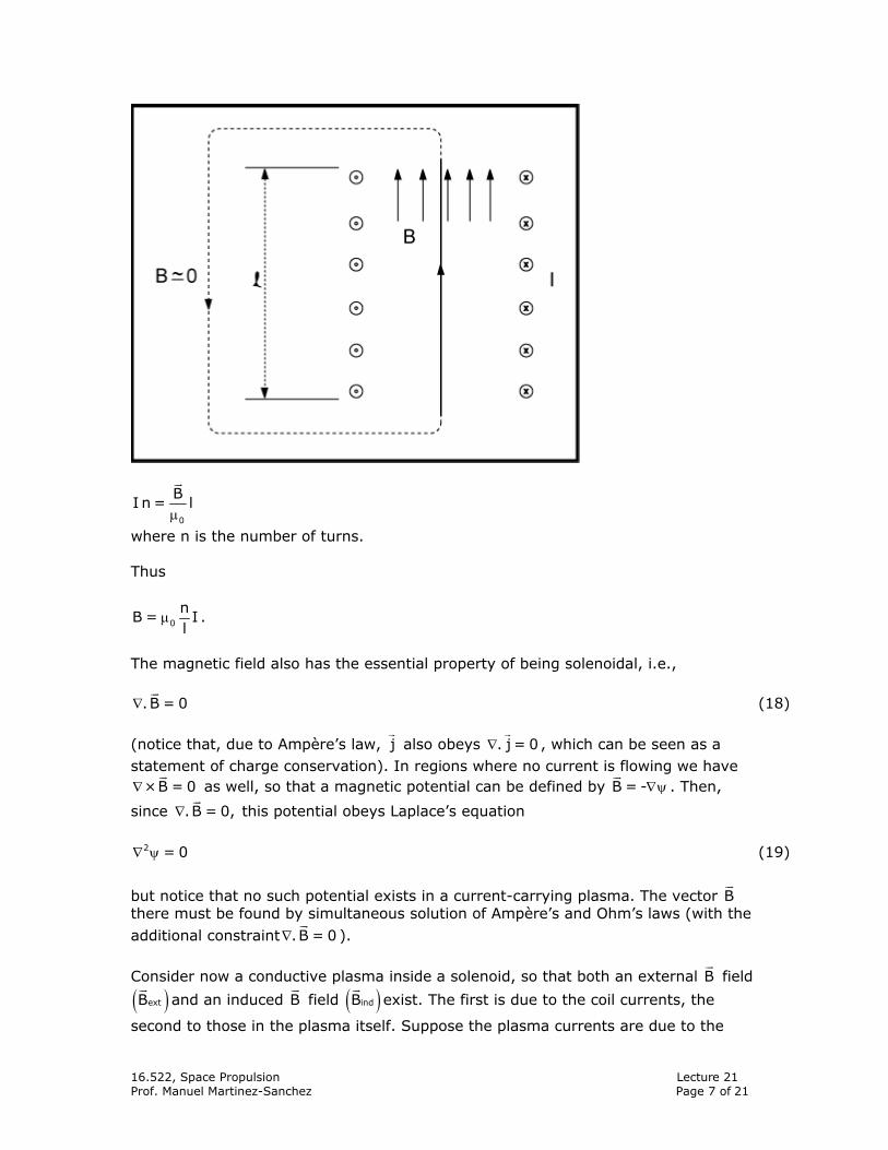
linked by the loop. When the current is constrained to circulate in metallic wires, the integral form can be used to provide simple formulae for the field due to various conductor arrangements. For example, inside a long solenoid carrying a current I, the field B is nearly constant, and we obtain (see sketch)


0

BI n = l

µ

where n is the number of turns. Thus

0

nB = I

lµ .

The magnetic field also has the essential property of being solenoidal, i.e.,

. B = 0∇ (18)

(notice that, due to Ampère’s law, j also obeys . j = 0∇ , which can be seen as a statement of charge conservation). In regions where no current is flowing we have

× B = 0∇ as well, so that a magnetic potential can be defined by B = -∇ψ . Then,

since . B = 0,∇ this potential obeys Laplace’s equation

2 = 0∇ ψ (19) but notice that no such potential exists in a current-carrying plasma. The vector B there must be found by simultaneous solution of Ampère’s and Ohm’s laws (with the

additional constraint . B = 0∇ ). Consider now a conductive plasma inside a solenoid, so that both an external B field

( )extB and an induced B field ( )indB exist. The first is due to the coil currents, the

second to those in the plasma itself. Suppose the plasma currents are due to the


flow at uof the plasma in the total magnetic field B , while any external electrodes

are short-circuited, so that E = 0 in the laboratory frame. Then E' = E+u × B = u × B . In order of magnitude, E' u B . Neglecting the Hall effect, then, j u Bσ ∼ .

The induced field obeys separately its own Ampère’s law ind

0

B× = j∇

µ, where j is the

plasma current density; this is because ext× B = 0∇ in the plasma (outside the coil wires). Thus, in order of magnitude

ind 0B j lµ∼ where l is the characteristic distance for variation indB ,i.e., the plasma “size.” Altogether,

ind 0B l u B µ σ∼ (20)

0 indB = B +B , so

ind0

ind 0

B l u

B +Bµ σ∼

This indicates that the field created by the plasma currents becomes comparable to the external field when the so-called “magnetic Reynolds number”

em 0R = l uµ σ (21) becomes of order unity. For a high power Argon MPD accelerator,

1000 mho/m, u 10,000 m/sec, l 0.1 m,σ ∼ so

-6 -1 3 4emR 10 × 10 × 10 × 10 = 1∼

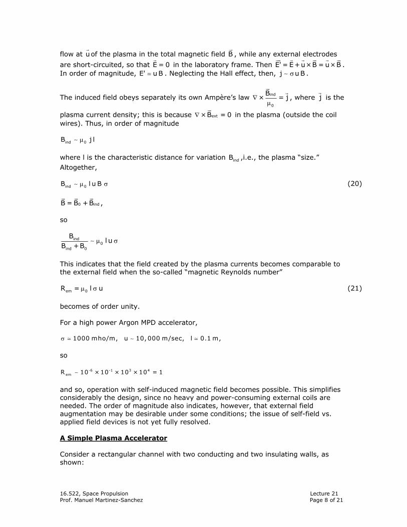
and so, operation with self-induced magnetic field becomes possible. This simplifies considerably the design, since no heavy and power-consuming external coils are needed. The order of magnitude also indicates, however, that external field augmentation may be desirable under some conditions; the issue of self-field vs. applied field devices is not yet fully resolved. A Simple Plasma Accelerator Consider a rectangular channel with two conducting and two insulating walls, as shown:


A plasma is flowing in the channel at velocity u , and an external electric field is

applied. Ignoring for now the Hall effect, if this E field is larger in magnitude than uB (the induced Faraday field), a current j will flow,

given by ( )j = E' = E+u × Bσ σ in the direction of E .

The Lorentz force f = j × B is then in the forward direction, as indicated, and we have an accelerator.

On the other hand, if E<uB, the current j flows in

the direction opposite to E . Externally, positive current flows into the (+) pole of our “battery” and could be used to recharge it; we have now an MHD generator, and the battery would probably be replaced by a passive load. The Lorentz force now points backwards, so that the fluid has to be forced

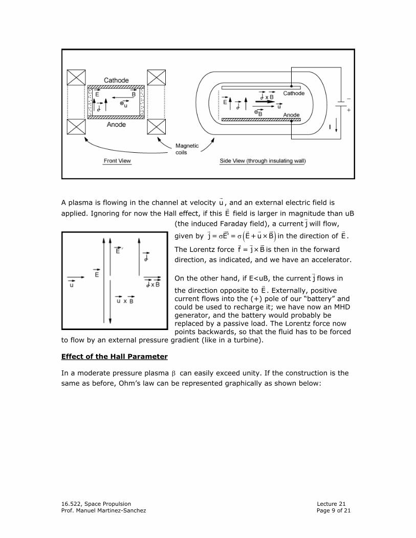
to flow by an external pressure gradient (like in a turbine). Effect of the Hall Parameter In a moderate pressure plasma β can easily exceed unity. If the construction is the same as before, Ohm’s law can be represented graphically as shown below:


We can see that the effect is to turn the current and the Lorentz force counter clockwise by arc tanβ . There is still a forward force (called the “blowing” force), but also now a transverse force, called the “pumping” force, because its main effect is to pump fluid towards the cathode wall, creating a transverse pressure gradient (low pressure at the anode). Basically, the axial (or Hall) current does no useful work, but it still contributes to the Joule dissipation 2j σ . Thus, we may want to turn the whole

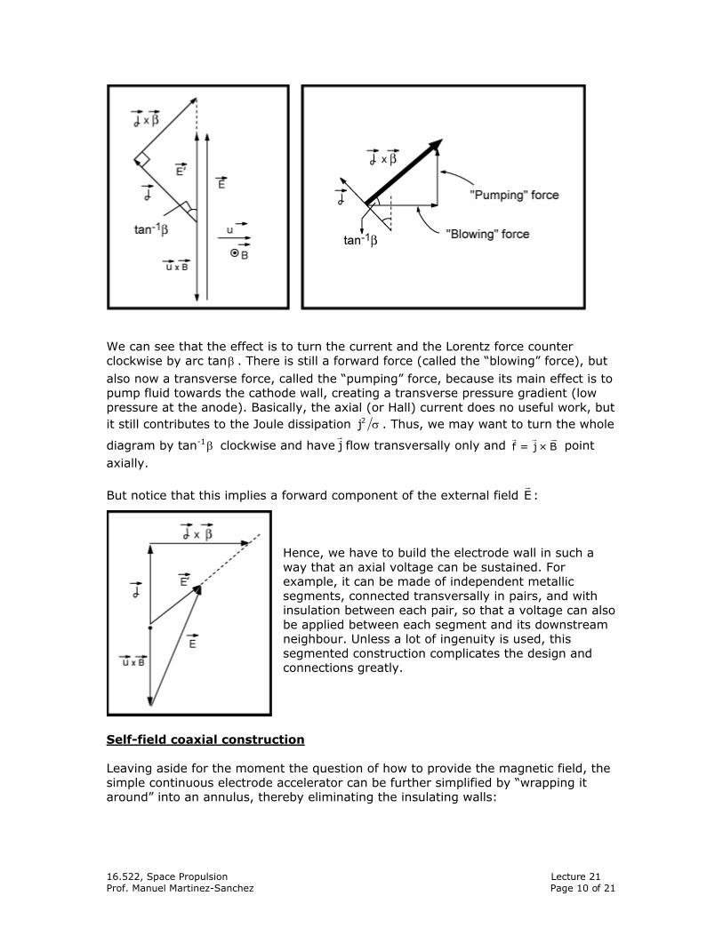
diagram by tan-1 β clockwise and have j flow transversally only and f = j × B point axially. But notice that this implies a forward component of the external field E :

Hence, we have to build the electrode wall in such a way that an axial voltage can be sustained. For example, it can be made of independent metallic segments, connected transversally in pairs, and with insulation between each pair, so that a voltage can also be applied between each segment and its downstream neighbour. Unless a lot of ingenuity is used, this segmented construction complicates the design and connections greatly.

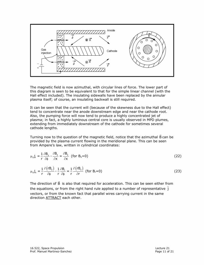
Self-field coaxial construction Leaving aside for the moment the question of how to provide the magnetic field, the simple continuous electrode accelerator can be further simplified by “wrapping it around” into an annulus, thereby eliminating the insulating walls:


The magnetic field is now azimuthal, with circular lines of force. The lower part of this diagram is seen to be equivalent to that for the simple linear channel (with the Hall effect included). The insulating sidewalls have been replaced by the annular plasma itself; of course, an insulating backwall is still required. It can be seen that the current will (because of the skewness due to the Hall effect) tend to concentrate near the anode downstream edge and near the cathode root. Also, the pumping force will now tend to produce a highly concentrated jet of plasma; in fact, a highly luminous central core is usually observed in MPD plumes, extending from immediately downstream of the cathode for sometimes several cathode lengths. Turning now to the question of the magnetic field, notice that the azimuthal B can be provided by the plasma current flowing in the meridional plane. This can be seen from Ampere’s law, written in cylindrical coordinates:

x0 r

B BB1j = - =

r x xφ φ∂ ∂∂

µ∂φ ∂ ∂

(for Bx=0) (22)

( ) ( )r0 x

rB rBB1 1 1j = - =

r r r rφ φ∂ ∂∂

µ∂φ ∂φ ∂

(for Br=0) (23)

The direction of B is also that required for acceleration. This can be seen either from

the equations, or from the right hand rule applied to a number of representative j vectors, or from the known fact that parallel wires carrying current in the same direction ATTRACT each other.


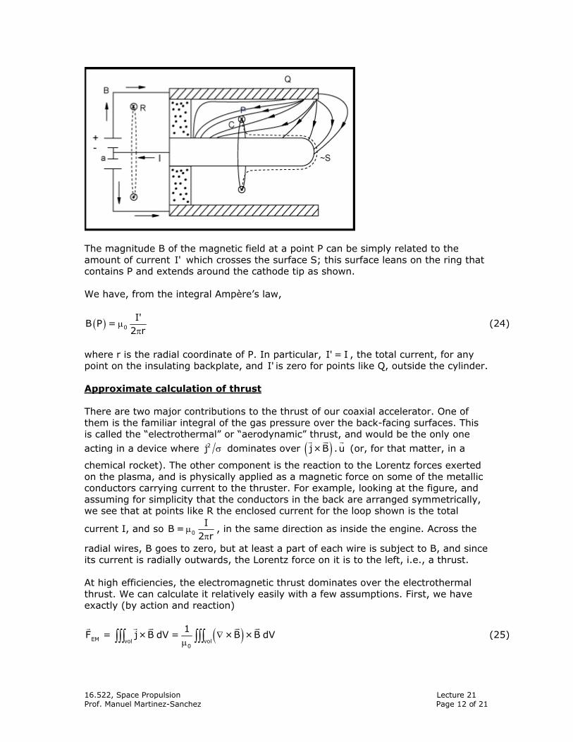
The magnitude B of the magnetic field at a point P can be simply related to the amount of current I' which crosses the surface S; this surface leans on the ring that contains P and extends around the cathode tip as shown.

We have, from the integral Ampère’s law,

( ) 0

I'B P =

2 rµ

π (24)

where r is the radial coordinate of P. In particular, I' = I , the total current, for any point on the insulating backplate, and I' is zero for points like Q, outside the cylinder. Approximate calculation of thrust There are two major contributions to the thrust of our coaxial accelerator. One of them is the familiar integral of the gas pressure over the back-facing surfaces. This is called the “electrothermal” or “aerodynamic” thrust, and would be the only one

acting in a device where 2j σ dominates over ( )j × B . u (or, for that matter, in a

chemical rocket). The other component is the reaction to the Lorentz forces exerted on the plasma, and is physically applied as a magnetic force on some of the metallic conductors carrying current to the thruster. For example, looking at the figure, and assuming for simplicity that the conductors in the back are arranged symmetrically, we see that at points like R the enclosed current for the loop shown is the total

current I, and so 0

IB =

2 rµ

π, in the same direction as inside the engine. Across the

radial wires, B goes to zero, but at least a part of each wire is subject to B, and since its current is radially outwards, the Lorentz force on it is to the left, i.e., a thrust.

At high efficiencies, the electromagnetic thrust dominates over the electrothermal thrust. We can calculate it relatively easily with a few assumptions. First, we have exactly (by action and reaction)

( )EM vol vol0

1F = j × B dV = × B × B dV∇

µ∫∫∫ ∫∫∫ (25)


In general

( ) ( ) ( )2× B × B = B B - B 2∇ ∇ ∇ (26)

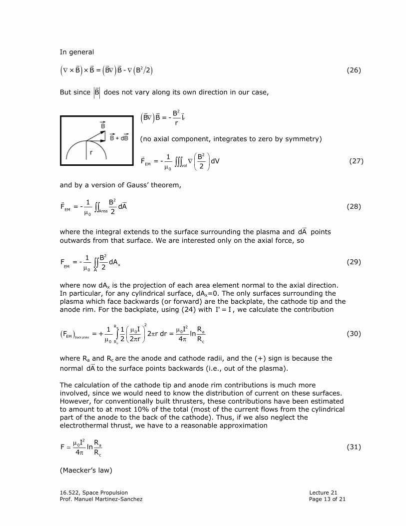
But since B does not vary along its own direction in our case,

( )2

rB

B B = - lr

∇

(no axial component, integrates to zero by symmetry)

2

EM vol0

1 BF = - dV

2⎛ ⎞

∇ ⎜ ⎟µ ⎝ ⎠∫∫∫ (27)

and by a version of Gauss’ theorem,

2

EM Area0

1 BF = - dA

2µ ∫∫ (28)

where the integral extends to the surface surrounding the plasma and dA points outwards from that surface. We are interested only on the axial force, so

2

xEM0 A

1 BF = - dA

2µ ∫∫ (29)

where now dAx is the projection of each area element normal to the axial direction. In particular, for any cylindrical surface, dAx=0. The only surfaces surrounding the plasma which face backwards (or forward) are the backplate, the cathode tip and the anode rim. For the backplate, using (24) with I' = I , we calculate the contribution

( )a

Back plate

c

2R 20 0 a

EM0 cR

I I R1 1F = + 2 r dr = ln

2 2 r 4 Rµ µ⎛ ⎞

π⎜ ⎟µ π π⎝ ⎠∫ (30)

where Ra and Rc are the anode and cathode radii, and the (+) sign is because the

normal dA to the surface points backwards (i.e., out of the plasma). The calculation of the cathode tip and anode rim contributions is much more involved, since we would need to know the distribution of current on these surfaces. However, for conventionally built thrusters, these contributions have been estimated to amount to at most 10% of the total (most of the current flows from the cylindrical part of the anode to the back of the cathode). Thus, if we also neglect the electrothermal thrust, we have to a reasonable approximation

20 a

c

I RF ln

4 Rµ

π (31)

(Maecker’s law)


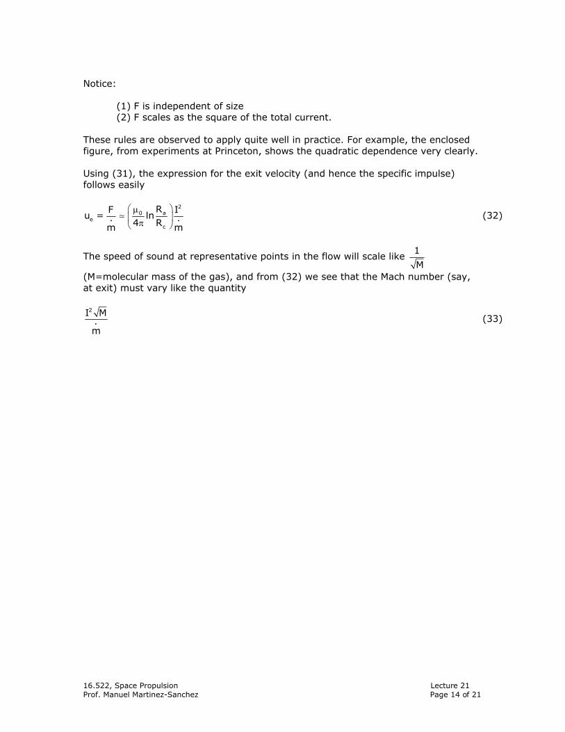
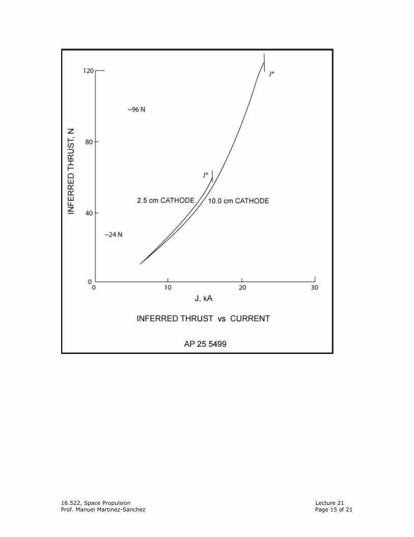
Notice:

(1) F is independent of size (2) F scales as the square of the total current.

These rules are observed to apply quite well in practice. For example, the enclosed figure, from experiments at Princeton, shows the quadratic dependence very clearly. Using (31), the expression for the exit velocity (and hence the specific impulse) follows easily

20 a

ec

RF Iu = ln

4 Rm m

⎛ ⎞µ⎜ ⎟π⎝ ⎠

i i (32)

The speed of sound at representative points in the flow will scale like 1

M

(M=molecular mass of the gas), and from (32) we see that the Mach number (say, at exit) must vary like the quantity

2I M

mi (33)




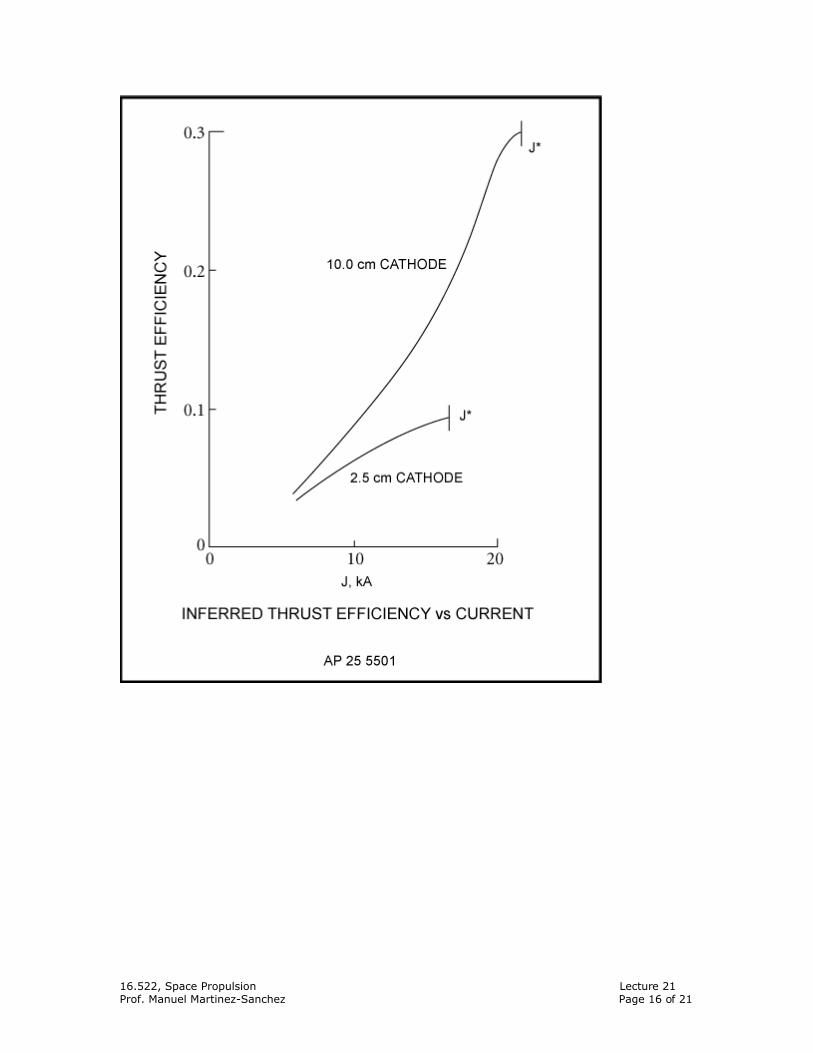
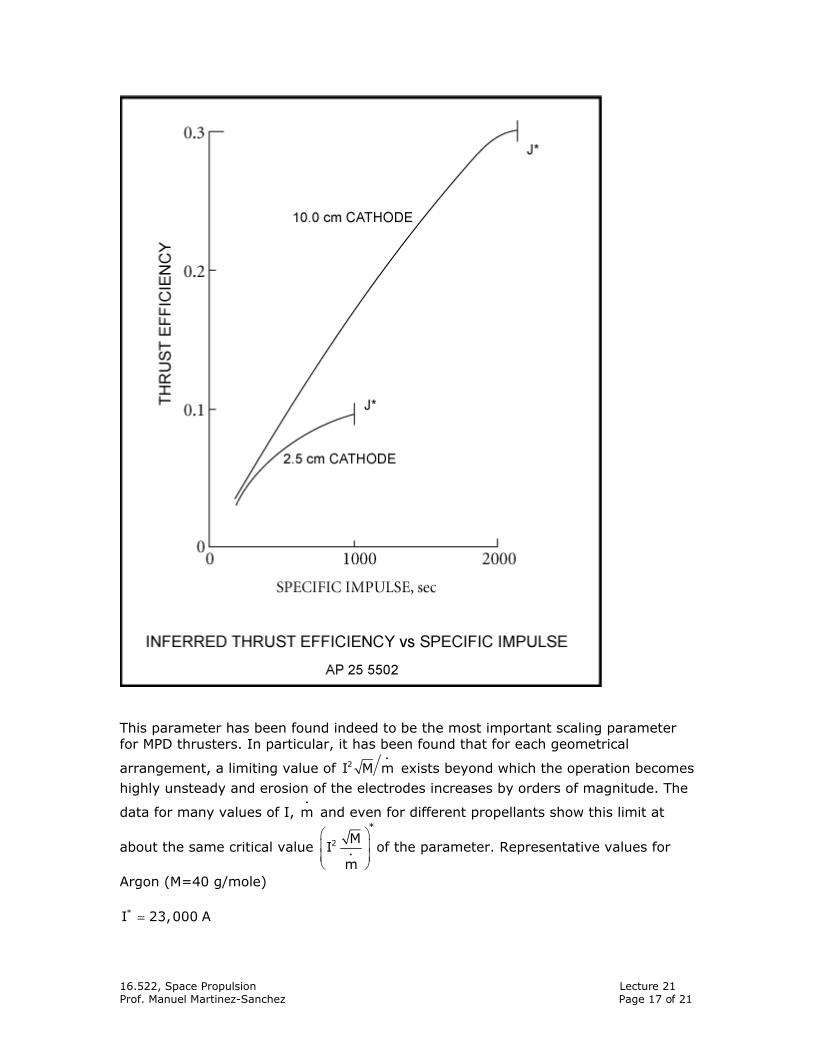
This parameter has been found indeed to be the most important scaling parameter for MPD thrusters. In particular, it has been found that for each geometrical

arrangement, a limiting value of 2I M mi

exists beyond which the operation becomes highly unsteady and erosion of the electrodes increases by orders of magnitude. The

data for many values of I, mi

and even for different propellants show this limit at

about the same critical value 2

*M

Im

⎛ ⎞⎜ ⎟⎜ ⎟⎝ ⎠

i of the parameter. Representative values for

Argon (M=40 g/mole)

*I 23,000 A


*

m 6 g/seci

giving

*

2 MI 560 (I in KA, M in g/mole,m in g/sec)

m

⎛ ⎞⎜ ⎟⎜ ⎟⎝ ⎠

i

i .

However, this limit can be modified by changes in the configuration of the engine, and much research is being done to push it to as high values as possible. The reason is that as this parameter increases, so does the ratio of magnetic pressure

2 20B 2 Iµ to dynamic pressure

mmu

M

ii

∼ ∼ , and hence, the relative importance of

electromagnetic effects. Thus, high values of 2I M

mi lead to high thruster efficiency,

and (as shown by Equation (32)) high specific impulse. The electrical characteristics of the accelerator can also be estimated from Equation (31). If the thrust efficiency is

22e

1 F mmu 12= =I V 2 I V

⎛ ⎞⎜ ⎟⎝ ⎠η

ii

,

then, using (31) we obtain

2 30 a

c

R1 IV = ln

2n 4 R m

⎛ ⎞µ⎜ ⎟π⎝ ⎠

i (34)

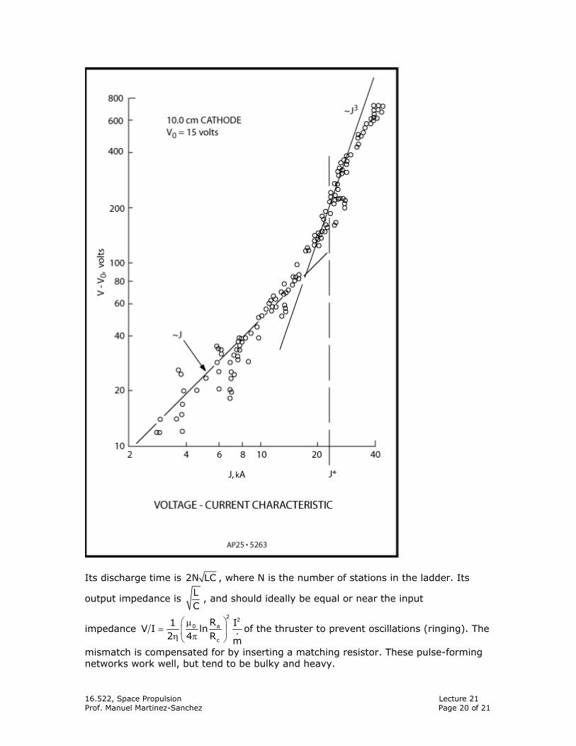
Thus, if η itself varies little with current, the voltage is seen to vary as the cube of the current. This trend is indeed observed at high currents (see graph, from Princeton tests). At lower currents, η does go down, and in addition the electrothermal component of thrust predominates, and the near-electrode voltage drops become comparable to the voltage needed for acceleration. The net result is a departure from the 3V I∼ line, towards a linear dependence. Power Requirements Consider the 2300 Amp, 6 g/sec example mentioned before, and assume Rc=1 cm, Ra=5 cm. The thrust is then

( )2-7 5F =10 × 23000 ln = 85.1 Nt

1

and the jet power is


( )225

jet

85.1FP = = = 6.04×10 Watt

2×0.0062mi

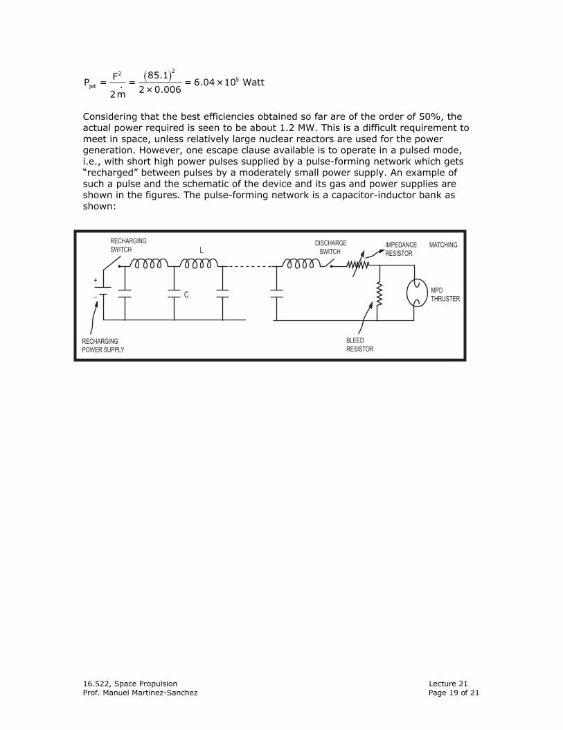
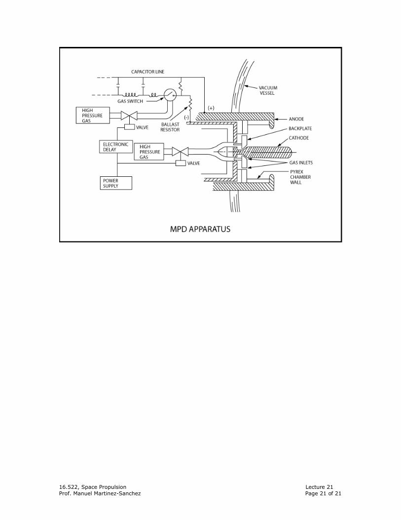
Considering that the best efficiencies obtained so far are of the order of 50%, the actual power required is seen to be about 1.2 MW. This is a difficult requirement to meet in space, unless relatively large nuclear reactors are used for the power generation. However, one escape clause available is to operate in a pulsed mode, i.e., with short high power pulses supplied by a pulse-forming network which gets “recharged” between pulses by a moderately small power supply. An example of such a pulse and the schematic of the device and its gas and power supplies are shown in the figures. The pulse-forming network is a capacitor-inductor bank as shown:

C

L

+

−

RECHARGINGSWITCH

RECHARGINGPOWER SUPPLY

BLEED RESISTOR

DISCHARGE SWITCH

IMPEDANCE RESISTOR

MATCHING

MPDTHRUSTER


Its discharge time is 2N LC , where N is the number of stations in the ladder. Its

output impedance is LC

, and should ideally be equal or near the input

impedance 2 2

0 a

c

R1 IV I ln

2 4 R m

⎛ ⎞µ⎜ ⎟η π⎝ ⎠

i of the thruster to prevent oscillations (ringing). The

mismatch is compensated for by inserting a matching resistor. These pulse-forming networks work well, but tend to be bulky and heavy.


Documents

Prof. Lecture 21: Electrostatic versus Electromagnetic