Professional Consequences of Couple Internal Migration: Evidence from France

Ariane PailhéIned

133 bd. Davout75020 Paris

Francetél : 33 (0)1 56 06 22 74fax : 33(0)1 56 06 21 99

pailhe@ined.fr

Anne SolazIned

133 bd. Davout75020 Paris

Francetél : 33 (0) 1 56 06 21 30fax : 33 (0) 1 56 06 21 99

solaz@ined.fr

Summary:This article examines the impact of internal migration on dual­earner couples’ labor market participation and earnings in France. The analysis is based on longitudinal data from the French version of  the European Community Household Panel.  Internal mobility   is  a   rare event   in France,  specially   for   couples.  Controlling   for   self­selection   of  migrants,   results   show  that household income diminishes the year following migration, as the probability to be employed, strongly for women. Once controlling for the market labor participation, migration has a positive impact on male income, but not on female one. The year after, migration is more profitable, but essentially for men, meaning that women are often the ‘tied movers’. The rigidity of the French labor market associated with a high level of unemployment may explain both the difficulty and the weak benefit to move in couple.

Keywords:Internal migration, couple, gender, income, labor market participation

IntroductionThe  researches on professional outcome of migration are  largely  individual­centered. Their implicit hypothesis is that the mobility decision is taken by the working partner belonging to single­earner   couples,   or   that   the   decision­making   process   is   driven   by   the   head   of   the household (or  the partner with  the higher wage)  in dual­earner couples. Results  show that migration behaviors differ  according  to  sex.  Traditionally,  men have a  greater professional mobility   that   can be  explained by   their   smaller   familial   responsibilities,   their   smaller  risk aversion or their larger job search area. With   increasing   women   labor   force   participation,   such   assumptions   about   the   migration decision process seem less valid. It seems obvious that moving is a couple decision ­or even a family decision since it implies all the family members. This joint decision for the couple may be the result of a bargaining process between spouse, the economic power of each partners being determinant. 

Moreover, the migration may have different consequences for both partners in terms of labor market participation, job type or earnings. For instance, among people who have stopped a former job for personal reasons in  the survey we use,  the reason “my partner has  to move because of his/her job” is declared in 15% of cases for women against only 4% for men. This figure points  out   that   couple migration  could  have  different  impact  for  partners  according his/her sex.The purpose of this article is to examine the migration decision process while taken the couple as a unit of analysis, and to measure the professional consequences of couple internal migration. It studies  the influence of migration on spouses  labor market participation,  total household income and the relative earnings of partners. How do each partner’s characteristics play on the family decision to move?  How does migration affect the labor market participation of each partner? How does the migration affect the household and individual earnings and the earning gap between partner? While answering those questions, we will take into account the potential correlation   between   unobserved   household   characteristics   exerting   influence   on   both   the decision to migrate and on outcomes.This paper is structured in the following way. It first provides a short review of the literature and of earlier researches linking household migration, labor market participation and income. Next section presents both   the database and  the  method used. Then  it  gives   the  results  on  the determinants  of mobility and  its  outcomes  in  terms of employment and  income. The final section provides some concluding comments. 

Background and previous researchMost researches on the determinants and consequences of migration are based on the human capital theory. In that framework, people maximize their lifetime utility and migration is viewed as a human capital investment (Polachek and Horvath, 1977). Individuals migrate when the long terms returns exceed the moving costs (monetary and non monetary costs like loss of social networks, neighborhood knowledge). DaVanzo (1976), Sandell (1977) and Mincer (1978) were the first to consider family migration decision­making. In that traditional unitary model, the spouses have a single utility function, male and female income are pooled, and the household well­being does not depend on the intra­household resource allocation. The spouses maximize this single utility function when taking the decision to migrate. According to Mincer's  initial model, the household migrates  if  the household net benefit of migration (gains less costs) is positive. This optimum reached at the household level may differ from the optimum people would have reached at the individual level. One spouse’s post migration individual income may decrease whereas the household income increases. As women’s market power is generally lower than their  partner’  one, women are likely to be ‘tied movers’, i.e. they move although they wouldn’t have moved if the migration decision have been taken on a individual basis, because their income would have been higher by staying. In that case, migration reinforce earnings gap between the spouses. On the other hand, men are more often ‘tied stayers’, i.e. they do not migrate although they would have increased their individual earning while moving. This is more likely when their partner contributes to the household  income  in   a   large  proportion and  when women  have  a   continuous career path. Finally,  as   couples have   to  consider  both  spouses outcomes,  spouses  are   less  mobile   than singles.Empirical studies, mainly conducted on American panel data, tend to support the human capital model of migration. Several researches confirm that dual­earner couples are less mobile than single­earner couples (Long, 1974; Mincer, 1978; Nivalainen, 2004). Moreover, women tend to 

2

follow their partner whereas the reverse is less likely (Markham and Pleck, 1986 ; Shihadeh, 1991).   After   migration,   their   professional   prospects   worsen:   they   are   more   likely   to   be unemployed or out of labor force (Boyles et al, 2001 ; Duncan and Perrucci, 1976; LeClere and McLaughlin, 1997), and employment quality decreases (Morrison and Lichter, 1988). But these results   depend  on   the   local   job  market   of   the   arrival   location,   since  a  mobility   toward   a extensive job market may encourage female careers (Bonney and Love, 1991). The majority of researches   found   that   migration   deteriorates   female   incomes  (Bird   and   Bird,   1985).   This negative impact, stronger for educated women, is mainly due to a reduction of working hours (LeClere and McLaughlin, 1997) and is recovered two years later (Lichter, 1983 ; Spitze, 1984). On  the contrary,  migration generally   involves  an  increase  in male  incomes  (Sandell, 1977; Cooke, 2003). There is no consensus in the literature concerning the migration impact on the household income. Sandell (1977) and Cooke (2003) found a positive effect, while it is not significant for Axelsson and Westerlund (1998), and negative for Jacobsen and Levin (1997). From the Survey on Income and Program Participation, they show that the migration returns depend on the macro­economic situation of the country. Some migrants are obliged to move because of   their  weak opportunities   in   their   starting country   (« push  effect »),   rather   than because they are attracted by better perspectives (« pull effect »). 

A more recent and growing literature move away from the human capital model of migration. New  theoretical   models,   the   collective   models,   analyse   interactions   between   spouses   who maximize separate utilities. Lundberg and Pollack (2003) have developed a non cooperative model of family migration. As the location may affect future relative bargaining of spouses, some migration will not occur even if the family income would increase after a move. One spouse may refuse migration when its bargaining position is weakened after migration. Finally, some papers place gender roles at the core of the migration decision process. Some researches show that women mobility patterns and outcomes do not differ from men’s ones in the absence of traditional gender role, e.g. in case of lesbian same­sex couples (Cooke, 2005) or equalitarian couples in terms of housework allocation (Bielby and Bielby, 1992; Jürges, 2005). Other researches point out the asymmetry between men and women in the  family migration decision making.  For instance, Duncan and Perruci (1976) and Lichter (1982) point up that female characteristics do not explain the migration process, on the contrary to men’s ones. However,  Rabe  (2006), using an estimate corrected  for  selection of both  participation and migration, shows that dual­earner couples weight equally each partners expected wages in the decision process.  

Like in other European countries, French internal migration is relatively weak compared to the United States (Long, 1992). It may be explained by higher costs of moving, the labor market rigidity, the high rate of unemployment, the weak return of migration and the dominant model of dual­earner households. The literature dealing with the returns of migration in France focuses on   individual   migration   (Simmonet,   1996,   Drapier   and   al.,   2002).   It   shows   that   internal migration favours male career path (Arrighi and Roux, 2006). The sole research dealing with family migration was based on the tree­years panel of the labor force survey. It finds that the higher   the   migration   distance,   the   higher   probability   one   spouse   become   inactive   or unemployed, particularly women. It shows that migration does not favour women to find a job while unemployed before migration (Courgeau, Meron, 1995).

Data and Methodology

3

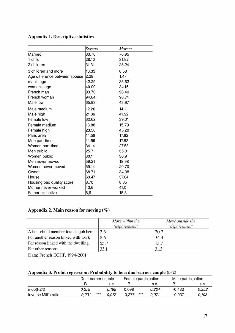
DataThe data  used  in   this   study comes  from  the  French  version of   the   longitudinal  European Community Household Panel (ECHP). This survey carried out by the French National Institute of Statistics (INSEE) contains eight waves, from 1994 to 2001. All household members aged 17 and more are interviewed at one­year interval, in October. This panel is individual based, i.e. all people interviewed in the first wave were approached the waves after, conditionally not being absent   two   years   in   succession.   The   panel   contains   yearly   information   regarding   socio­demographic characteristics, professional status, individual and household income, housing and mobility. A total of 7,344 households (14,332 adults) were initially interviewed, they were 5345 households (9,218 adults) in the last wave. Individuals were followed up in case of move or decohabitation, except   if   they move abroad or  in   institution.  Attrition  is  higher  in  case of moving, however more than eight individuals out of ten answers after moving (Breuil­Genier et alii, 2000). This non­answering after moving is greater in case of couple splits, which are out of scope since we are interested in intact household moves.  We pooled the eight panel waves in one large data set, which counts 63,212 year­observations of individuals. We keep all individuals in age to participate to the labor market from 17 to 60 years old,  except   students  and  retired people. The  idea  is   to   avoid  spatial  move associated with completing education or entering retirement. Rather than focusing on individuals, our sample covers couples living in the same household, being married or not, who report family income. As Boyles et alii (2001), we need to use the household as a unit of analysis if we are interested in the impact of migration when couples had moved together. We do not restrict the analysis to dual­earner  couples,  in  order  to   include people who experience employment  status  change during the migration period. It also minimizes sample selection bias related to labor market participation.   Finally,   our   sample   contains   22,887   year­observation   couples.  Sample characteristics are given in the appendix 1.

DefinitionsWe focus here on long­distance migration (within France) of couples. A migration is defined as occurring when a household changes his ‘département’1 of residence between two yearly waves of   the   survey,   rather   than  just  moving between  counties  within   a   department,   or  between residence within a county. We focus here on long distance migrations that are more likely to be linked with employment rather than other reasons like housing conditions, etc2. Indeed, when asking people the reason of moving, the professional reason is advanced in 55% of cases when the   household   move   outside   the  département  against   11%   in   case   of   move   within   the département3 (appendix 2). Migration is a quite rare event in France: only 3.7% of singles and 1.8% of couples experienced a move outside the département during in a two­years interval. Migration is more frequent when one spouse does not work: 1.6% of dual­earner couples had moved and 1.9% of single­earner couples. 

1 France is divided into 95 areas called “départements”. A département change is a quite significant change since it implies new local government, schools, car registration plate, etc… 2  An   inter   departmental   migration   is   not   necessary   a   long   distance   move.   We   have   distinguished   border départements migration from migration farer. The results obtained are very similar as those with our definition which was kept because the sample was larger. 3 This information if given in the survey on a household basis. Unfortunately, we do nor have this information for each spouse, which could have been a way to identify tied and lead migrants..

4

We measure different migration outcomes. On the one hand, we are first interested in spouses labor force participation, whether both spouses work after migration (dual­earner couple). On the other hand, we study the influence of migration on income. We examine three measures of income and earnings: 

The family income which is family’s average monthly income4; The  individual  average  monthly   income which   is  made up  of  wages,   income  from 

secondary activity, income from self­employment, parental leave benefit, unemployment and other benefits;

The  individual average monthly wage for people who are working as wage earners (including bonuses);

The men’s share in the couple income related with labor market participation (wage, unemployment benefit, work pension, etc.). 

Like Axelsson and Westerlund (1996), we consider changes in real incomes rather than nominal income. Earnings are expressed in 2001 euros and in logarithms.

Selection BiasLong distance migration is often related to job opportunities and wages incentives. Workers would get different incomes in different areas because local job markets are differentiated and workers' skill can be rewarded differently  in each area (Gobillon & Leblanc, 2003). In  this context, selection into migrants and non migrants may be non random: migrants may differ from stayers in observed and unobserved characteristics witch also affect participation and wages (Borjas, 1987; Guillermin, Rosenzweig, 1990). For instance, level of education, age, but also individual   dynamism,   polyvalence   or   language   knowledge   may   explain   both   the   moving behavior and the wage level. Migration is thus a self­selection process and movers and stayers’ earnings are not randomly selected. We correct from these possible selection biases (Nakosteen, Zimmer, 1980; Vella 1997) and endogeneity problem. A two­stage model according to the Heckman’s method (Heckman, 1979; Axelsson, Westerlund, 1998 for an application) is used. We first estimate the probability that the couple moves outside the current department. Secondly, we analyze the consequences of the couple migration in terms of labor market participation and income. 

Econometric specificationThe econometric specification is the following. First we estimate the migration equation using a probit model. 

(1) 

≤=>=

0001

*

*

ii

ii

MifM

MifM

with  iii eYM += '* γMi   is equal to 1 if the couple migrates outside the department and 0 otherwise. Yi is a set of explanatory variables for the migration benefit Mi

*, which is a latent variable   “expressing” the propensity to migrate. We assume that ei are normally distributed.The   migration  equation   includes  socio­demographic   characteristics   such   as   marital   status, number of children, the age of the head, the age difference between spouses, the education level of each spouse. We distinguish three levels of education: high for people who get a university diploma, medium for people who get a secondary diploma and low for others. Employment 4 Information related to earnings are collected on an annual basis. We have computed a monthly average amount.

5

status  is  added: dummies variables  indicting whether  the man does not work, whether  the woman is unemployed or out of the labor force. Some variables are linked with the dwelling: one   binary   variable   indicates   home   ownership,   one   its   dilapidation.   As   instruments,   we introduce the type of dwelling (house or not) and the migration history, i.e. each spouse has moved from his/her birth department or not and. All of these variables are measured at t­1. We control also by the year and type of settlement (large urban area or not).

The probit estimation (1) provides estimation for  '.γ̂  Then  )'ˆ( iYγφ  and  )'ˆ( iYγΦ which are respectively the density and distribution function of normal law, can be computed. The inverses of Mills ratios follow the formulas:

 (2) )'ˆ()'ˆ(ˆ

1i

ii Y

Yγγφλ

Φ= for couples who migrate (Mi=1)

)'ˆ(1)'ˆ(ˆ

0i

ii Y

Yγ

γφλΦ−

−=  for couples who do not migrate (Mi=0)

We then estimate models on the professional consequences of migration on participation to the labour market Pi , household income I and wages Wf and Wh. 

The models are the following: (3) Pi= iiii uMX +++ χαλβ(4) Ii= iiii uMX +++ χαλβ(5) Wf= fiif uMX +++ χαλβ   and Wh= hiih uMX +++ χαλβwith Xi  the characteristics of the household, and Xf   and Xh  the characteristics of respectively the female and male partner. 

 is the parameter effect of the selection effect. If the unobserved characteristics of migrants (orα  non   migrants)   are   correlated   to   the   unobserved   characteristic   of   explained   variables,   the selection should be corrected and   will be significantly different of 0. αχ is   the  parameter   of   the  migration  effect,   once  corrected  the   selection  effect   and other characteristics.  

ResultsThe probability of couple migrationThe migration probability is modeled as a function of individual, labor­market and housing characteristics of the couple in the year prior to that in which a move could have occurred (table 1). The results show that being married has no impact on the probability of migration whereas the presence of children reduces it. The number of children living in the household, more than their age, weaken the migration strategies. Man’s age tends to reduce it5, which is a common result   to  most  migration  studies.  As  expected,  the  probability  of  migration  increases with education for both partners since more highly educated individuals would tend to have a better information about non local  job opportunities and may be more adaptable to change. Once controlled   for   individual   characteristics,   the   employment   status   of   each   partner   has   no significant impact on the probability of moving. 

5 Only the husband’s age is included given the high correlation in spouses’ age.

6

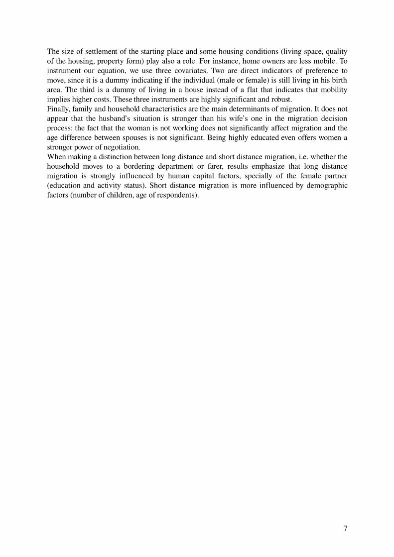
The size of settlement of the starting place and some housing conditions (living space, quality of the housing, property form) play also a role. For instance, home owners are less mobile. To instrument our equation, we use three covariates. Two are direct  indicators of preference to move, since it is a dummy indicating if the individual (male or female) is still living in his birth area. The third is a dummy of living in a house instead of a flat that indicates that mobility implies higher costs. These three instruments are highly significant and robust. Finally, family and household characteristics are the main determinants of migration. It does not appear that the husband’s situation is stronger than his wife’s one in the migration decision process: the fact that the woman is not working does not significantly affect migration and the age difference between spouses is not significant. Being highly educated even offers women a stronger power of negotiation. When making a distinction between long distance and short distance migration, i.e. whether the household moves   to  a  bordering department  or   farer,   results   emphasize  that   long distance migration  is   strongly   influenced by  human capital   factors,   specially   of   the   female partner (education and activity status). Short distance migration is more influenced by demographic factors (number of children, age of respondents).

7

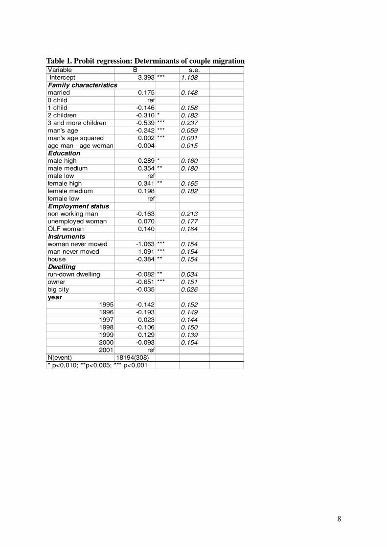
Table 1. Probit regression: Determinants of couple migration

8

Variable B s.e. Intercept 3.393 *** 1.108Family characteristicsmarried  0.175 0.1480 child ref1 child  ­0.146 0.1582 children  ­0.310 * 0.1833 and more children   ­0.539 *** 0.237man's age  ­0.242 *** 0.059man's age squared 0.002 *** 0.001age man ­ age woman  ­0.004 0.015Education male high 0.289 * 0.160male medium 0.354 ** 0.180male low reffemale high 0.341 ** 0.165female medium 0.198 0.182female low refEmployment statusnon working man  ­0.163 0.213unemployed woman 0.070 0.177OLF woman 0.140 0.164Instrumentswoman never moved  ­1.063 *** 0.154man never moved  ­1.091 *** 0.154house  ­0.384 ** 0.154Dwellingrun­down dwelling  ­0.082 ** 0.034owner  ­0.651 *** 0.151big city  ­0.035 0.026year  

1995  ­0.142 0.1521996  ­0.193 0.1491997 0.023 0.1441998  ­0.106 0.1501999 0.129 0.1392000  ­0.093 0.1542001 ref

N(event) 18194(308)* p<0,010; **p<0,005; *** p<0,001

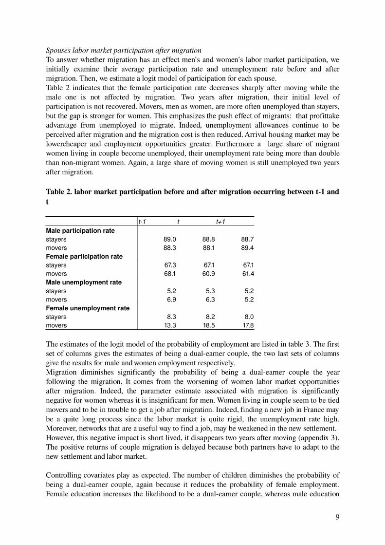
Spouses labor market participation after migrationTo answer whether migration has an effect men’s and women’s labor market participation, we initially   examine   their   average   participation   rate   and   unemployment   rate   before   and   after migration. Then, we estimate a logit model of participation for each spouse.Table 2 indicates that the female participation rate decreases sharply after moving while the male   one   is   not   affected   by   migration.   Two   years   after   migration,   their   initial   level   of participation is not recovered. Movers, men as women, are more often unemployed than stayers, but the gap is stronger for women. This emphasizes the push effect of migrants:  that profittake advantage   from unemployed   to  migrate.   Indeed,   unemployment  allowances  continue  to   be perceived after migration and the migration cost is then reduced. Arrival housing market may be lowercheaper and employment opportunities greater.  Furthermore a    large share of migrant women living in couple become unemployed, their unemployment rate being more than double than non­migrant women. Again, a large share of moving women is still unemployed two years after migration.

Table 2. labor market participation before and after migration occurring between t­1 and t

  t­1 t t+1Male participation rate    stayers 89.0 88.8 88.7movers 88.3 88.1 89.4Female participation ratestayers 67.3 67.1 67.1movers 68.1 60.9 61.4Male unemployment ratestayers 5.2 5.3 5.2movers 6.9 6.3 5.2Female unemployment ratestayers 8.3 8.2 8.0movers 13.3 18.5 17.8

The estimates of the logit model of the probability of employment are listed in table 3. The first set of columns gives the estimates of being a dual­earner couple, the two last sets of columns give the results for male and women employment respectively. Migration   diminishes   significantly   the   probability   of   being   a   dual­earner   couple   the   year following the migration. It comes from the worsening of women labor market opportunities after   migration.   Indeed,   the   parameter   estimate   associated  with   migration   is   significantly negative for women whereas it is insignificant for men. Women living in couple seem to be tied movers and to be in trouble to get a job after migration. Indeed, finding a new job in France may be a quite  long process since  the  labor market  is  quite  rigid,  the unemployment rate high. Moreover, networks that are a useful way to find a job, may be weakened in the new settlement. However, this negative impact is short lived, it disappears two years after moving (appendix 3). The positive returns of couple migration is delayed because both partners have to adapt to the new settlement and labor market. 

Controlling covariates play as expected. The number of children diminishes the probability of being a dual­earner couple, again because it reduces the probability of female employment. Female education increases the likelihood to be a dual­earner couple, whereas male education 

9

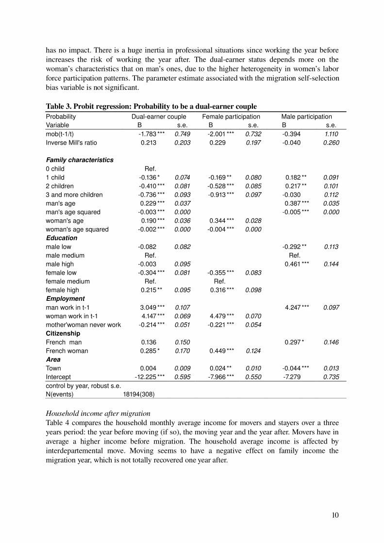
has no impact. There is a huge inertia in professional situations since working the year before increases  the   risk  of  working  the  year   after.  The dual­earner   status  depends more  on   the woman’s characteristics that on man’s ones, due to the higher heterogeneity in women’s labor force participation patterns. The parameter estimate associated with the migration self­selection bias variable is not significant. 

Table 3. Probit regression: Probability to be a dual­earner coupleProbability Dual­earner couple Female participation Male participationVariable B   s.e. B   s.e. B   s.e.mob(t­1/t) ­1.783 *** 0.749 ­2.001 *** 0.732 ­0.394 1.110Inverse Mill's ratio 0.213 0.203 0.229 0.197 ­0.040 0.260

Family characteristics0 child Ref.1 child ­0.136 * 0.074 ­0.169 ** 0.080 0.182 ** 0.0912 children ­0.410 *** 0.081 ­0.528 *** 0.085 0.217 ** 0.1013 and more children  ­0.736 *** 0.093 ­0.913 *** 0.097 ­0.030 0.112man's age 0.229 *** 0.037 0.387 *** 0.035man's age squared ­0.003 *** 0.000 ­0.005 *** 0.000woman's age 0.190 *** 0.036 0.344 *** 0.028woman's age squared ­0.002 *** 0.000 ­0.004 *** 0.000Education male low ­0.082 0.082 ­0.292 ** 0.113male medium Ref. Ref.male high ­0.003 0.095 0.461 *** 0.144female low ­0.304 *** 0.081 ­0.355 *** 0.083female medium Ref. Ref.female high 0.215 ** 0.095 0.316 *** 0.098Employment man work in t­1 3.049 *** 0.107 4.247 *** 0.097woman work in t­1 4.147 *** 0.069 4.479 *** 0.070mother'woman never work ­0.214 *** 0.051 ­0.221 *** 0.054CitizenshipFrench  man  0.136 0.150 0.297 * 0.146French woman  0.285 * 0.170 0.449 *** 0.124AreaTown 0.004 0.009 0.024 ** 0.010 ­0.044 *** 0.013Intercept ­12.225 *** 0.595 ­7.966 *** 0.550 ­7.279 0.735control by year, robust s.e.                  N(events) 18194(308)              

Household income after migrationTable 4 compares the household monthly average income for movers and stayers over a three years period: the year before moving (if so), the moving year and the year after. Movers have in average   a   higher   income  before   migration.   The   household  average   income  is   affected  by interdepartemental   move.   Moving   seems  to   have   a   negative   effect   on   family   income  the migration year, which is not totally recovered one year after. 

10

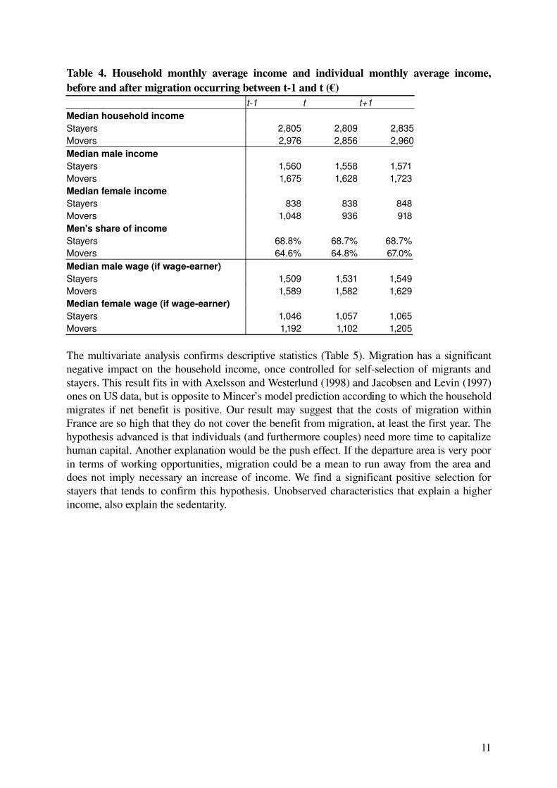
Table  4.  Household  monthly  average   income and  individual  monthly  average   income, before and after migration occurring between t­1 and t (€)  t­1 t t+1Median household income    Stayers 2,805 2,809 2,835Movers 2,976 2,856 2,960Median male income    Stayers 1,560 1,558 1,571Movers 1,675 1,628 1,723Median female incomeStayers 838 838 848Movers 1,048 936 918Men's share of incomeStayers 68.8% 68.7% 68.7%Movers 64.6% 64.8% 67.0%Median male wage (if wage­earner)    Stayers 1,509 1,531 1,549Movers 1,589 1,582 1,629Median female wage (if wage­earner)Stayers 1,046 1,057 1,065Movers 1,192 1,102 1,205

The multivariate analysis confirms descriptive statistics (Table 5). Migration has a significant negative impact on the household income, once controlled for self­selection of migrants and stayers. This result fits in with Axelsson and Westerlund (1998) and Jacobsen and Levin (1997) ones on US data, but is opposite to Mincer’s model prediction according to which the household migrates if net benefit is positive.  Our result may suggest that the costs of migration within France are so high that they do not cover the benefit from migration, at least the first year. The hypothesis advanced is that individuals (and furthermore couples) need more time to capitalize human capital. Another explanation would be the push effect. If the departure area is very poor in terms of working opportunities, migration could be a mean to run away from the area and does not imply necessary an increase of income. We find a significant positive selection for stayers that tends to confirm this hypothesis. Unobserved characteristics that explain a higher income, also explain the sedentarity. 

11

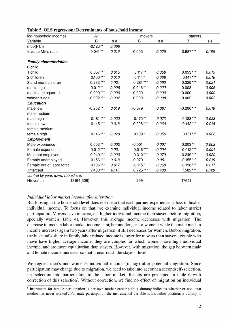
Table 5. OLS regression: Determinants of household incomelog(household income) All movers stayersVariable B     s.e. B     s.e. B     s.e.mob(t­1/t) ­0.123 ** 0.066Inverse Mill's ratio 0.041 ** 0.019 ­0.005 0.025 0.987 *** 0.185

Family characteristics0 child1 child 0.057 *** 0.015 0.117 ** 0.058 0.053 *** 0.0152 children 0.150 *** 0.016 0.114 * 0.068 0.147 *** 0.0163 and more children  0.233 *** 0.021 0.281 *** 0.090 0.229 *** 0.021man's age 0.012 ** 0.006 0.046 ** 0.022 0.008 0.006man's age squared 0.000 *** 0.000 0.000 0.000 0.000 0.000woman's age ­0.002 *** 0.002 0.000 0.008 ­0.002 0.002Education male low ­0.202 *** 0.019 ­0.079 0.067 ­0.206 *** 0.019male mediummale high 0.181 *** 0.022 0.170 ** 0.073 0.183 *** 0.023female low ­0.145 *** 0.018 ­0.228 *** 0.060 ­0.142 *** 0.018female mediumfemale high 0.146 *** 0.020 0.109 * 0.056 0.151 *** 0.020Employment Male experience 0.003 ** 0.002 ­0.001 0.007 0.003 ** 0.002Female experience 0.012 *** 0.001 0.016 *** 0.004 0.012 *** 0.001Male not employed ­0.249 *** 0.020 ­0.310 *** 0.079 ­0.249 *** 0.020Female unemployed ­0.156 *** 0.018 ­0.070 0.051 ­0.155 *** 0.019Female out of labor force ­0.196 *** 0.017 ­0.115 * 0.060 ­0.198 *** 0.017 Intercept 7.480 *** 0.117 6.725 *** 0.403 7.582 *** 0.120control by year, town, robust s.e.                 N(events) 18194(308)     299     17641    

Individual labor market income after migrationBut loosing at the household level does not mean that each partner experiences a loss in his/her individual income. To focus on that, we examine individual income related to labor market participation. Movers have in average a higher individual income than stayers before migration, specially   women   (table   4).   However,   this   average   income   decreases   with   migration.   The decrease in median labor market income is higher and longer for women: while the male median income increases again two years after migration, it still decreases for women. Before migration, the husband’s share in family labor related income is lower for movers than stayers: couple who move have higher average income, they are couples for which women have high individual income, and are more equalitarian than stayers. However, with migration, the gap between male and female income increases so that it near reach the stayers’ level. 

We  regress men’s  and women’s  individual  income (in  log) after potential  migration. Since participation may change due to migration, we need to take into account a secondself­ selection, i.e.   selection  into  participation  to   the   labor  market.  Results   are presented  in   table 6  with correction of this selection6. Without correction, we find no effect of migration on individual 6  Instrument for female participation is her own mother career path: a dummy indicates whether or not ‘own mother has never worked’. For male participation the instrumental variable is his father position: a dummy if 

12

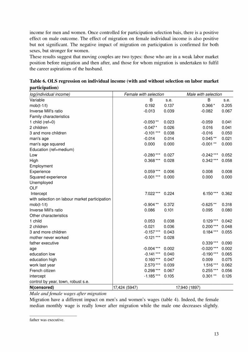
income for men and women. Once controlled for participation selection bais, there is a positive effect on male outcome. The effect of migration on female individual income is also positive but not significant. The negative impact of migration on participation is confirmed for both sexes, but stronger for women. These results suggest that moving couples are two types: those who are in a weak labor market position before migration and then after, and those for whom migration is undertaken to fulfil the career aspirations of the husband.     Table 6. OLS regression on individual income (with and without selection on labor market participation)log(individual income) Female with selection Male with selectionVariable B     s.e. B     s.e.mob(t­1/t) 0.192 0.137 0.366 * 0.205Inverse Mill's ratio ­0.013 0.039 ­0.082 0.067Family characteristics1 child (ref=0) ­0.050 ** 0.023 ­0.059 0.0412 children ­0.047 * 0.026 0.016 0.0413 and more children  ­0.101 *** 0.038 ­0.016 0.050man's age ­0.014 0.014 0.045 ** 0.021man's age squared 0.000 0.000 ­0.001 ** 0.000Education (ref=medium)Low ­0.280 *** 0.027 ­0.242 *** 0.052High 0.368 *** 0.028 0.342 *** 0.058Employment Experience 0.059 *** 0.006 0.008 0.008Squared experience ­0.001 *** 0.000 0.000 0.000UnemployedOLF Intercept 7.022 *** 0.224 6.150 *** 0.362with selection on labour market participation            mob(t­1/t) ­0.904 ** 0.372 ­0.625 ** 0.318Inverse Mill's ratio 0.086 0.101 0.095 0.080Other characteristics1 child 0.053 0.038 0.129 *** 0.0422 children ­0.021 0.036 0.200 *** 0.0483 and more children  ­0.157 *** 0.043 0.184 *** 0.055mother never worked ­0.121 *** 0.028father executive 0.339 *** 0.090age ­0.004 *** 0.002 ­0.020 *** 0.002education low ­0.141*** 0.040 ­0.190 *** 0.065education high 0.160 *** 0.047 0.009 0.075work last year 2.570 *** 0.039 1.516 *** 0.062French citizen 0.298 *** 0.067 0.255 *** 0.056intercept ­1.185 *** 0.105 0.301 ** 0.126control by year, town, robust s.e.             N(censored) 17,424 (5947)     17,940 (1897)  Male and female wages after migrationMigration have a different impact on men’s and women’s wages (table 4). Indeed, the female median monthly wage is really lower after migration while the male one decreases slightly. 

father was executive. 

13

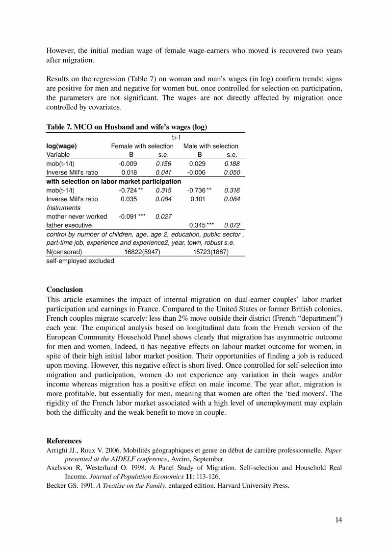
However, the initial median wage of female wage­earners who moved is recovered two years after migration. 

Results on the regression (Table 7) on woman and man’s wages (in log) confirm trends: signs are positive for men and negative for women but, once controlled for selection on participation, the  parameters  are not   significant. The wages are not  directly  affected by  migration once controlled by covariates.  

Table 7. MCO on Husband and wife’s wages (log)  t+1log(wage) Female with selection Male with selectionVariable B     s.e. B     s.e.mob(t­1/t) ­0.009 0.156 0.029 0.188Inverse Mill's ratio 0.018 0.041 ­0.006 0.050with selection on labor market participation    mob(t­1/t) ­0.724 ** 0.315 ­0.736 ** 0.316Inverse Mill's ratio 0.035 0.084 0.101 0.084Instrumentsmother never worked ­0.091 *** 0.027father executive 0.345 *** 0.072control by number of children, age, age 2, education, public sector ,  part­time job, experience and experience2, year, town, robust s.e. N(censored) 16822(5947) 15723(1887)self­employed excluded

Conclusion This article examines the impact of internal migration on dual­earner couples’ labor market participation and earnings in France. Compared to the United States or former British colonies, French couples migrate scarcely: less than 2% move outside their district (French “department”) each year. The empirical analysis based on longitudinal data from the French version of the European Community Household Panel shows clearly that migration has asymmetric outcome for men and women. Indeed, it has negative effects on labour market outcome for women, in spite of their high initial labor market position. Their opportunities of finding a job is reduced upon moving. However, this negative effect is short lived. Once controlled for self­selection into migration and participation, women do  not  experience any variation  in   their wages and/or income whereas migration has a positive effect on male income. The year after, migration is more profitable, but essentially for men, meaning that women are often the ‘tied movers’. The rigidity of the French labor market associated with a high level of unemployment may explain both the difficulty and the weak benefit to move in couple.

ReferencesArrighi JJ., Roux V. 2006. Mobilités géographiques et genre en début de carrière professionnelle. Paper 

presented at the AIDELF conference, Aveiro, September.Axelsson  R,  Westerlund O.  1998.  A Panel  Study of  Migration.  Self­selection and Household  Real 

Income. Journal of Population Economics 11: 113­126.Becker GS. 1991. A Treatise on the Family. enlarged edition. Harvard University Press. 

14

Bielby WT, Bielby DD. 1992. I Will Follow Him: Family Ties, Gender­Role Beliefs, and Reluctance to Relocate for a Better Job. American Journal of Sociology 97: 1241­1267. 

Bird GG., Bird GW. 1985. Determinants of Mobility in Two­Earners Families; Do Wives’ Jobs Matters?. Journal of Marriage and the Family 47: 753­758.

Bonney N,  Love   J.   1991.  Gender   and  Migration:  Geographical  Mobility   and   the  Wife’s  Sacrifice. Sociological Review 39: 335­348.

Borjas GJ. 1987. Self Selection and the Earnings of Immigrants. The American Economic Review 77(4): 531­553. 

Borjas SG, Bronars SG. 1991. Immigration and the Family. Journal of Labor Economics 9(2): 123­148.Boyles P,.  Cooke TJ, Halfacree K, Smith D. 2001.   A Cross­National Comparison of  the Impact of 

Family Migration on Women’s Employment Status. Demography 38(2): 201­213.Breuil­Genier P, Legendre N, Valdelièvre H. 2000. Panel d’individus versus panel de logement, ou: que 

peut­on dire de la qualité du panel européen ?. Journées de méthodologie statistique, décembre. Cooke TJ. 2003. Family Migration and the Relative Earnings of Husbands and Wives.  Annals of the 

Association for American Geographers 3(3): 278­294.Cooke TJ. 2005. Migration of same­Sex Couples. Population, Space and Place 11(5): 401­409.Courgeau D, Meron M. 1995. Mobilité résidentielle. activité et vie familiale des couples.  Economie et 

statistique. 290: 17­31.DaVanzo  J.  1976.  Why   families   move:   A   model   of   the   mobility   of   married   couples.   The   RAND 

corporation, R­1976­DOL.DaVanzo J, Hosek J. 1981. Does Migration Increase Wage Rates? An Analysis of Alternative techniques 

for Measuring Wage gains to Migration N­1582­NICHD. Santa Monica: the Rand Corporation. July.

Drapier C, Jayet H. 2002. Les migrations des jeunes en phase d’insertion professionnelle en France. Une comparaison par niveau de qualification. Revue d’économie rurale et urbaine 3: 353­376.

Duncan RP, Perrucci CC. 1976. Dual Occupation Families and Migration. American Sociological review 41(2): 252­261.

Gobillon L. 2001. Emploi. logement et mobilité résidentielle. Economie et Statistique. 349­350: 77­98.Gobillon L, Le Blanc D. 2003. Migrations, Income and Skills. CREST Working Paper n°2003­47 Heckman J. 1979. Sample Selection Bias as a Specification Error. Econometrica. January. 153­162.Jacobsen JP, Levin LM. 1997. Marriage and Migration: Comparing Gains and Losses from Migration for 

Couples and Singles. Social Sciences Quarterly. 78(3): 688­709.Jasso  G,  Rosenzweig  MR.  1990.  Self­selection  and   the  Earnings  of   Immigrants   :  Comment   .  The 

American Economic Review 80(1): 298­304.Jürges H. 2005. Gender Ideology.  Division of Housework. and Geographic Mobility Families.  MEA 

discussion Paper series n°05090. Keith K, McWilliams A. 1997. Job Mobility and Gender­Based Wage Growth Differentials.  Economic 

Inquiry 35: 320­333.LeClere   FB,   McLaughlin   DK.   1997.   Family   migration   and   changes   in   women’s   earnings:   A 

decomposition analysis. Population Research and Policy Review 16: 315­335.Lichter DT. 1982. The migration of dual­worker families: Does the wife’s job matter?  Social Science 

Quarterly  63(1):48­57.Lichter DT. 1983. Socioeconomics Returns to Migration among Married Women.  Social Forces.  62: 

487­503.Light A, Ureta M. 1990. Gender Differences in Wages and Job Turnover Among Continuously Employed 

Workers in Women's Labor Market Mobility: Evidence from the NLS. The American Economic Review 80(2): 293­297.

Long L.H. 1974. Women’s Labor Force Participation and the Residential Mobility of Families. Social Forces. 52(3):342­348.

Long L. 1992.  Changing Residence:  Comparative Perspectives on its  Relationship  to Age, Sex,  and Marital Status. Population Studies 46(1):141­158.

15

Lundberg S, Pollak RA.2003. Efficiency in Marriage. Review of Economics of the Household 1(3): 153­168

Markam W, Pleck J. 1986. Sex and Willingness to Move for Occupational Advancement: Some National Sample Results. Sociological Quarterly 27: 121­143.

Mincer J. 1978. Family Migration Decision. The Journal of Political Economy. 86(5): 749­773.Morrison   DR,   Lichter   DT.   1988.  Family   Migration   and   Female   Employment:   The   Problem   of 

Underemployment among Migrant married Women. Journal of Marriage and the Family 50: 161­172.

Nakosteen R.A. Zimmer M.A. 1980.  Migration and Income: the Question of Self­Selection.  Southern Economic Journal 46: 840­851.

Nivalainen   S.   2004.   Determinants   of   family   migration:   short   moves   vs.   long   moves.  Journal   of  Population Economics 17: 157­175.

Polachek SW, Horvath FW. 1977. A Life Cycle Approach to Migration: Analysis of the Perspicacious Peregrinator in  Research in Labor Economics.  Ehrenberg R. ed..  Greenwich. Conn.: JAI Press. 103­149.

Rabe   B.   2006.   Dual­earner   migration   in   Britain.   Earnings   gains,   employment,   and   self­selection. Institute for Social and Economic Research Working Paper 2006­01. 

Sandell  SH.  1977.  Women and the Economics  of  Family Migration  The Review of  Economics and Statistics 59(4): 406­414.

Shihadeh Edward S. 1991. The Prevalence of Husband­Centred Migration Employment Consequences for Married Mother. Journal of Marriage and the Family 55: 432­444.

Snaith J. 1990. Migration and Dual Career Households. in JH Johnson and J Salt eds. Labour Migration.  The Internal Geographical Mobility of Labour in the Developed World. David Fulton Publishers Ltd. London. 155­171. 

Spitze G. 1984. The Effect of Family Migration on Wives’ Employment: How Long Does it last?. Social  Sciences Quarterly. 65: 21­36.

Vella   F.   1997.  Estimating   Models   with   sample   Selection   Bias :   a   survey.  The   Journal   of   Human Resources. 33: 127­169.

16

Appendix 1. Descriptive statistics

Stayers MoversMarried 83.70 70.951 child 28.10 31.922 children 31.31 25.24

3 children and more 16.33 8.58Age difference between spouse 2.28 1.47man's age 42.29 35.62woman's age 40.00 34.15French man 93.70 96.40French woman 94.84 96.74Male low 65.93 43.97

Male medium 12.20 14.11Male high 21.86 41.92Female low 62.62 39.01Female medium 13.88 15.79Female high 23.50 45.20Paris area 14.59 17.82Men part­time   14.59 17.82Women part­time 34.14 27.53Men public 25.7 35.3Women public 30.1 36.9Men never moved 59.21 18.98Women never moved 59.14 20.70Owner 68.71 34.38House 69.47 37.64Housing bad quality score 8.70 8.05Mother never worked 43,6 41,0Father executive 8,6 15,3

Appendix 2. Main reason for moving (%) 

Move within the ‘département’

Move outside the ‘département’

A household member found a job here 2.6 20.7For another reason linked with work 8.6 34.4For reason linked with the dwelling 55.7 13.7For other reasons 33.1 31.3Data: French ECHP, 1994­2001

Appendix 3. Probit regression: Probability to be a dual­earner couple (t+2)Dual­earner couple Female participation Male participation

B   s.e. B   s.e. B   s.e.mob(t­2/t) 0,279 0,199 0,098 0,224 ­0,432 0,352Inverse Mill's ratio ­0,231 *** 0,073 ­0,277 *** 0,071 ­0,037 0,108

17