1

Representation and

Description

Representation and Description

• After Segmentation– We need to represent (or describe) the segmented

region– Representation is used for further processing– Often desire a compact representation

• That describes the object itself • Not necessarily its relation to the original image

– ie, position, orientation, etc. .

• Description– Provide useful descriptions of the region– Can be used for comparison, selection, etc

2

ExampleRepresentationChain Code Convex Hull

DescriptionArea = 5384Perimeter = 1023

Euler Number = -2

Some Desirable Features• Representations/Descriptions should be

invariant:– Translation– Rotation– Scale

• Similar regions should have the same description– regardless of their position or orientation in

the image• Note: this isn’t always possible

– But it is something to keep in mind

3

Representation Schemes

• Generally two approaches• Boundary Characteristics

– Represent region by external characteristics (ie, the boundary)

• Internal Characteristics– Represent region by internal

characteristics

Chain Codes

• Chain codes are used to represent a boundary– Uses a logically connected sequence of

straight-line segments– The line segments specify length and direction

• Direction coded using a number scheme– Based on N_4 or N_8 connectivity

4

Chain Codes

• Direction scheme

0

1

2

3

0

12

3

N_4 N_8

4

56

7

Chain Coding• Digital Images

– Pixels form an equally spaced grid in x and ydirection

– Chain coding can be created by following a boundary in some direction (say clockwise)

– assigning a direction to the segments connecting every pair of pixels

– assumes a 1-pixel wide boundary

5

Example

0, 0, 0, 3, 0, 0, 3, 3, 3, 3, 3, 2, 2, 2, 2, 2, 1, 1, 1, 1, 1, 1

Start

Chain Code

0

1

2

3N_4

Chain Coding• Translation invariant

– Note that this is different than a chain of (x,y) coordinates

– We are encoding the boundary itself

• Codes are sensitive to noise– If your boundary has some noise, this will show

up in the chain code– One solution

• Resample using a larger grid spacing• Also provides a more compact representation

6

Example

Original(Re-sampled at a lower resolution)

N_8 Boundary

Chain Code in Practice

• Chain Code depends on the starting point

• We can normalize the chain code to address this problem– Assume the chain is a circular sequence

• (given a chain of 1 to N codes ; N+1 = 1)– Redefine the starting point such that we

generate an integer of smallest magnitude

7

Normalized Code

0, 0, 0, 3, 0, 0, 3, 3, 3, 3, 3, 2, 2, 2, 2, 2, 1, 1, 1, 1, 1, 1

Start Start

3, 0, 0, 3, 3, 3, 3, 3, 2, 2, 2, 2, 2, 1, 1, 1, 1, 1, 1, 0, 0, 0

Chain Code 1 Chain Code 2

0, 0, 0, 3, 0, 0, 3, 3, 3, 3, 3, 2, 2, 2, 2, 2, 1, 1, 1, 1, 1, 1Normalized Code

Chain Code in Practice

• Chain code depend on orientation– a rotation results in a different chain code

• One solution– Use the “first difference” of the chain code

instead of the code itself• The difference is obtained by simply

counting (counter-clockwise) the number of directions that separate two adjacent elements

8

Difference Coding

0

1

2

3

N_4

Difference Code

Chain Code1 0 1 0 3 3 2 2

3 1 3 3 0 3 0

You can normalize the difference code too.

Difference: Count the numberof separating directions in an anti-clockwise fashion

2

3

Chain Coding• Not scale invariant

– You can provide several chain codes of the same object at difference “resolutions”

• While difference coding helps, it does not make a chain code completely invariant to rotation– Image digitization and noise can cause problems– Nonetheless, it is a fairly common encoding

scheme

9

Polygonal Approximations

• Represent the boundary as a polygonal structure– Since the region is of discrete points

• We can create an exact representation• Simply connect each pixel center

• However, we often want to reduce the exact representation by providing a more compact “approximation”

Polygonal Approximation Example

10

Polygonal Approximation• Challenge

– Determine which points on the boundary to use

• One technique is segment splitting– Start with a line between the two farthest

points on the boundary

– Find the maximum perpendicular distance from the boundary to this line

– sub-divide region (repeat)

Segment Splitting

11

Signatures• A signature is a 1-D function used to

describe a region – Often used to describe a 2-D boundary– The signature is often unique for a region

• We can distinguish the region by its signature

• One common technique – Use the distance from the centroid of the

region to the boundary as a function of angle– s(φ) =d

Signature Example

12

Signatures• Are not invariant to scale

– Scale results in a signature with greater magnitude

– We can normalize the magnitude– (by min and max magnitudes)

• Signature depends on starting point– This means they are not invariant to rotation– Solution, pick the same starting point (if

possible)• find the farthest away point, start there• this should be rotation invariant

Boundary Segments

• Idea:– Decompose the boundary into segments

– Select key features on the boundary

– Reduces the overall boundary complexity

13

Convex Deficiency• Convex Hull, H, of an arbitrary set, S, is

the smallest set containing S

• H minus S (H-S)– Is called the convex deficiency

• We can use the convex deficiency to mark features

• Follow the contour of S and mark points that transitions into or out of the convex deficiency

Example

Convex Hull

Convex Deficiency(Shaded Area)

14

Using Convex Hull and its Deficiency

• This data can be used to describe the region– Number of pixels in convex deficiency– Number of components in convex

deficiency– Ratio lengths of the transition points– so on

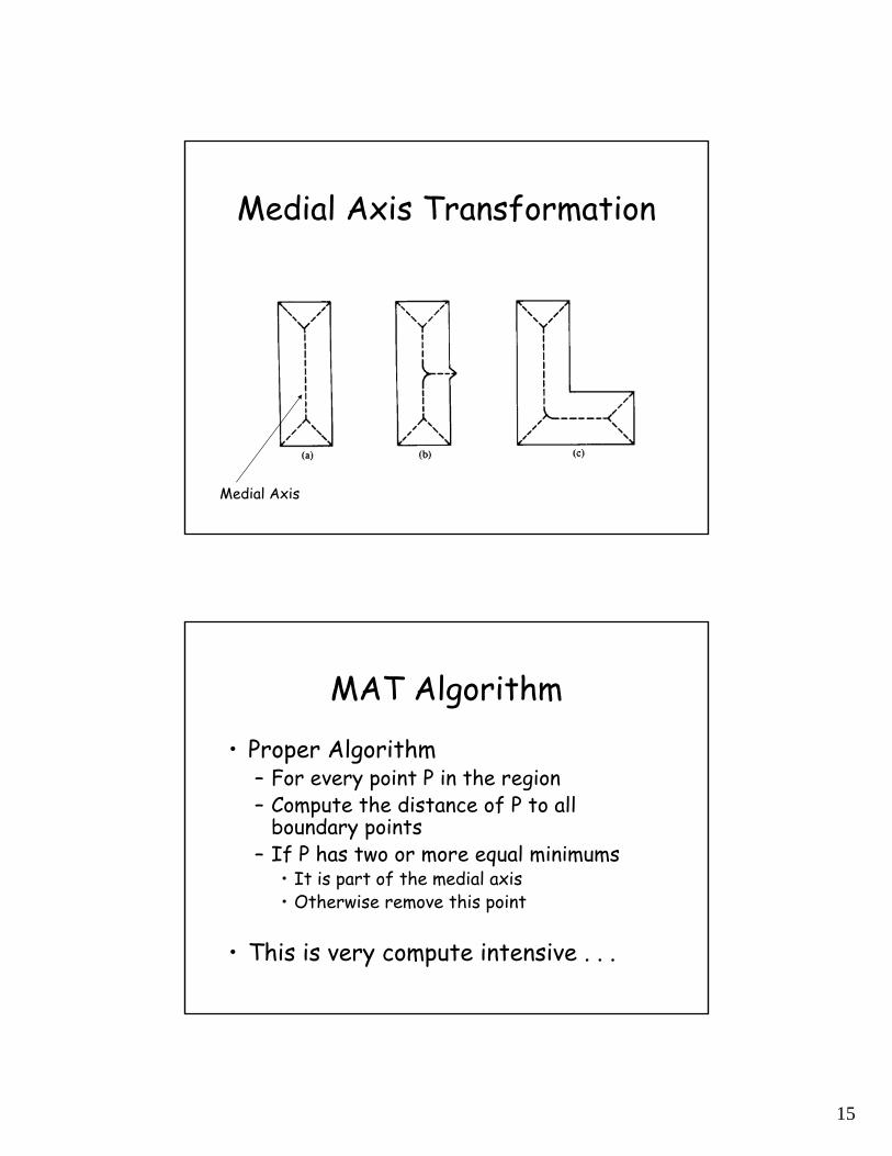
Skeleton of a Region• The skeleton of a region may be defined via the

Medial Axis Transformation (MAT)

• The MAT of a region R with border B is as follows– For each point p in R

• we find p’s closest neighbor in B• If p has more than one such neighbor, it is said to

belong to the medial axis

• Note: This definition depends on how we defined our distance measure (closest)

• Generally euclidean distance, but not a restriction

15

Medial Axis Transformation

Medial Axis

MAT Algorithm

• Proper Algorithm– For every point P in the region– Compute the distance of P to all

boundary points– If P has two or more equal minimums

• It is part of the medial axis• Otherwise remove this point

• This is very compute intensive . . .

16

Thinning Algorithm for approximating the MAT

• 2-pass approach– Assume foreground pixels = “1”– Background = “0”– Define a contour point to be any point

• that has at least one N_8 neighbor valued 0

• Consider this arrangement for the following algorithm:

p3p6p7

p4p1p8

p3p2p9

Thinning Algorithm (Non-MM algorithm)

• 1st pass– Flag a contour point p for deletion if the following conditions

are satisfied:(a) 2 <= N(p1) <= 6(b) S(p1) = 1;(c) p2 * p4 * p6 = 0(d) p4 * p6 * p8 = 0

– N(p1) is the number of nonzero neighbors of p1– S(p1) is the number of 0-1 transitions in the ordered

sequence of p2, p3, . . . , p8, p9, p2

• If (a) – (d) are not violated, the point is marked for deletion

– Points are not deleted until the end of the pass– This way the data stays intact until the pass is complete

17

• 2nd pass– Conditions (a) and (b) are the same as the 1st pass– (c) and (d) are different [call these (c’) and (d’)]:

(c’) p2 * p4 * p8 = 0(d’) p2 * p6 * p8 = 0

• Delete all points that are flagged from the 2nd pass

• Repeat this procedure until the image converges– IE, until you cannot remove any more pixels

Thinning Algorithm (Non-MM algorithm)

Thinning Algorithm• Algorithm info:

– if (a) is violated, this means this point is an “end-point”

– (b) is violated when p1 is on a stroke 1 pixel thick

– (c) and (d) are satisfied if • (p4 = 0 or p6 = 0) or (p2 = 0 and p8 = 0)

– (c’) and (d’) are satisfied if• (p2 =0 or p8=0) or (p4=0 and p6=0)

18

Example

Boundary Descriptors• Length of the contour

– Simply count the number of pixels along the border

– You may consider diagonally connected pixels to count as

• Diameter of the boundary B– Diam(B) = max[D(pi,pj)]– this is the major axis of the region

2

19

Boundary Descriptors• Curvature

– Rate of change of the slope

• Bounding Box– Smallest rectangle (aligned with the image axis)

that can bound the region

• Shape number– compute the chain code difference– re-order this to create the minimum integer– this is called the shape number

Shape Number Example

20

Shape Number

Compute the shapenumber using a 2Dgrid aligned to theobject.

Fourier Descriptors• Consider an N-point digital boundary in the xy plane

• This forms a coordinate pairs (xo, yo), (x1, y2), . . . ., (xn-1, yn-1)

• We can consider this as two vectors– x(k) = xk– y(k) = yk

• Furthermore– We could consider this a complex number– s(k) = x(k) + jy(k) where j=sqrt(-1)

21

Fourier Descriptors

Fourier Descriptors• Using the vector s(k)

• Compute the 1-D Discrete Fourier Transform

• a(u) is called the Fourier Descriptors of the region

• Note, that we can compute our original s(k) by:

∑−

=

−=1

0

/2)(1)(N

k

NukjeksN

ua π

∑−

=

=1

0

/2)()(N

k

Nukjeuaks π

22

Fourier Descriptors• Suppose, that instead of using all the a(u)’s, only

the first M coefficients are used. This is equivalent to setting a(u) = 0 for u > M-1.

• This is a more compact representation

• This procedure is also similar to a high-pass filter

• Now we can reconstruct the resulting s’(k) using a’(u)

FD Example

23

Fourier Descriptors

• We only need a few descriptors to capture the gross shape of the boundary

• We can compare low-order coefficients between shapes to see how similar they are

Regional Descriptors• Area of the region

– Number of pixels in the region

• Perimeter– Length of its boundary

• Compactness– (perimeter2)/area– Compactness is invariant to translation, rotation,

and scale– It is minimal for a disk-shaped region

24

Regional Descriptors• The previously mentioned regional

descriptors are often used with “blob”detection algorithms

– You can select or delete blobs based on these descriptors

– Especially “area” and compactness• For example, consider that you are looking for circles

with radius of 10 pixels

Topological Descriptors

• Topology– The study of properties of a figure that

are unaffected by any deformation– Assuming no tearing or joining

25

Topological Descriptors

• Count the connected components in a region

• Euler number, E, is a nice descriptor– E = C – H– where C is the number of connected

components– H is the number of holes

Topological Descriptors

Euler Number = 0 Euler Number = -1

26

Representation and Description

• This lecture introduces some basic approaches to represent or describe regions

• Such operations are between early vision and higher analysis– These representation/descriptions are used by higher-

level operators

• Matching descriptions/representation can be tricky

• Often use pattern recognition techniques

Summary• Representation

– Boundary-based• chain code, shape number• polygon approximation• signatures• Fourier descriptors• Boundary segments• Skeletons

– Region-based• Area, perimeter • Compactness• Topological descriptors

27

Active Research

• Descriptions are used with “recognition”techniques– Pattern recognition– Very active area– Application specific

• Fingerprint recognition

• This work is linked with AI– Computer Vision and Image Understanding– Vision is often classified as an area in AI