RESEARCH REPORTStatistical Reporting ServiceU.S. Department of Agriculture

A COMPARISON OF SEVERALREGRESSION MODELS FOR

FORECASTING PECAN YIELDS

by Chapman P. GleasonResearch DivisionResearch and Development Branch

NOVEMBER 1974

------.------------------

CONTENTS

SUMMARY .••.••.••••••••••• I •••••••••••••••••••••••••••••••••••••••••• i

I NTRO DUCT I ON •••.••.••••.••••••••••.•••..•••••.••.••.••.••.••.•..••••• i i

DATA COLLECT I ON PROCEDURES•••••••••••••••••••••••••••••••••••••••••• 1

B1ock Se 1ec t ion •.•••••.••••••••.•••••.••••.••••••.•.•••••.••••• 1

Samp1e Tree Se 1ect ion ••••••••••••••••.••••••••••••••••••••••••• 1

Samp1e Limb Se 1ect ion ••••..••••••••••••••••••••••••••••.••••••• 1

Samp 1e Limb Counts •••••••••••••••••••••••••••..•••••••••••••.•• 2

Photography Procedures •••••••••••••••••.•••••.•••••••••••.••••• 2

Counts of Nuts from Photographs ••.••••••••••••••••.•••••••••••• 2

Nut Droppage Prior to Harvest •••.•.•••.•••••...••••••.•••••••.• 3

Ha rves t Data ••••••..•••••.••••••••••••••••••••••••••••••••••••• 3

DATA EXPANSIONS ••••••• ' •••••••••••••••••••.••.••••••••.•••••••••••••. 5

Limb Exp ans i on s •••.•••••••••••••••••••••••••••••••••••••••••••• 5

Photog raphy Expans ions ••••••••••••••••••••••••••••••••••••••••• 5

Drop Expans ions •••••••••••••••••••••.•.•••.••••••••••••••••.•.• 7

RE SU LT5 ••••.••.••.••.••••••••••••••••••••••••••••.••.•.•••••••••••.• 8

General 8

Cor re 1at i on Coeff i c i ents ••••••••••••••••••••••••••••••••••••••• 8

Ana 1ys i s of Reg res s i on Mode 1s •••••••••••••••••••••••••••••••••• 12

DISCUSS ION OF RESULTS ••••••••••••••••••••••••••••••••••••••••••••••• 23

CONCLUS ION5 •••••••••••••••••••.••••••••••••••••••••••••••••••••••••• 26

RECOMMENDATIONS ••••••.•••••••••••••••••••.•••••••••••••••••••••••••• 26

REFERENCES•••••••••••••••••••••••••••••••••••••••••••••••••••••••••• 29

SUMMARY

Several different regression models are compared to determine which

are best for forecasting average yield per tree. Criteria are proposed

to determine which variables and ultimately which regression models are

better than others. Using the proposed criteriat a simple linear regres-

sion model using the number of nuts counted on photographs was found to

be "best". Reconmendations are made for further research. A new method of

expanding the number of nuts counted on photographs to the tree level is

also presented. The study was based upon data collected in 1972 in centraland southern Mississippi.

A COMPARISON OF SEVERAL REGRESSION MODELSFOR FORECASTING PECAN YIELDS

BYCHAPMAN P. GLEASON

INTRODUCTION

Research studies have shown that limb sampling and photographic

data collection procedures are promising methods of providing data with

which to forecast the average yield (number or weight of nuts) per tree.

Two different approaches to forecasting the average yield per tree

were proposed in 1971. The first involved using two simple linear regres-

sions---yield versus the number of nuts on sample limbs; and yield versus

the number of nuts on photographs. The second involves a multiple regression

approach to the forecasting problem---yield versus the number of nuts on

limbs and photographs. The research was aimed at answering two questions:

1. Which of the above approaches is better?2. If simple linear regression is as good as multiple regression,

which regression gives the best estimate of average yield per

tree?

From a cost standpoint, one variable may be easier and cheaper to

collect and provide more precise forecasts. Tests of statistical hypothesis

will be formulated to answer the first question.

C.V.'s will be compared to answer the second.

2Standard errors, R , and

------------------------ ---------------~-----------

DAT~ COLLECTION PROCEDURES

Block Selection:

Five block of Stuart variety pecans were subjectively selected in

two separate geographic areas of Mississippi. Three blocks were located

in central Mississippi (Hinds County), all managed by one operator. Two

additional blocks were located in the southwestern corner of the State

(Wilkinson County), each managed by different individuals.

Sample Tree Selection:

For each of the three blocks in Hinds County, the trees used in a

1971 research project were used again (Wood (8». In Wilkinson County

it was necessary to select four trees in each of the newly selected

blocks. A two-stage procedure was used to select the trees.

1. Two rows were randomly selected with equal probability of selection

for each row.

2. Within each selected row, two trees were randomly selected with

equal probability. In this approach, if rows are varying lengths

trees in short rows have a greater probability of selection thanthose in long rows.

Sample Limb Selection:

For each selected tree, the total number of accessible (reachable by

a six-foot ladder) sample limbs was enumerated and a 50 percent simple

random sample with equal probabilities of selection was taken. Sample limbs

were defined as those with cross-sectional area between 1.8 and 5.5 square

inches. For each tree, the total number of sample limbs (both accessible andinaccessible) was estimated using either bare tree mappings of limbs or bare

tree stero photographs.

limbs for the i-th tree.

Nj will denote the total estimated number of sample

The trees in Hinds County had stero photographs

2

taken in early April 1971. (Huddleston (4) describes the uses of photo-

graphy to estimate the total number of sample limbs.) Bare tree mappings

of limbs were made and used to estimate the total number of sample limbsfor the trees selected in Wilkinson County.

Sample limb Counts:For each tree, once the sample limbs were selected all nuts on the

limb were counted by tagging each cluster of fruit and counting the number

of nuts In each tagged cluster. This prevented counting errors and gave

an indication of monthly fruit droppage from the clusters.

Photography Procedures:To avoid the poor quality photography that plagued the research

efforts in 1970 and 1971, the following techniques were used:

1. The tripod which held the camera was located 50 feet from the

base of the tree with the sun at the back of the photographer.

2. A florist stake was placed directly below the tripod.

3. The metal photography frame was placed two feet in front of the

camera lens.

4. The angle of the camera from the tree was recorded.

The photographs were taken up a vertical column of the tree through

a metal frame. A Miranda Sensorex camera with an in-lens light meter

improved the photograph significantly over those with a camera which

has no in-lens light meter.

Counts of Nuts from Photographs:

Each slide was projected on a grid. The number of nuts in each cell

was counted by a photo interpreter. A certain subset of the slides was

recounted for computation of photo adjustments factors. (See Wood (7,p.19)

for a discussion of methods used to compute photo adjustment factors.)

----------------------~--~--_._-_._--------~-~_ .._------~-----------

Nut Droppage Prior to Harvest:

On the first photography visit, two square plots, each two feetby two feet, were randomly located on the ground beneath the canopy of

each tree. The identified area was then gleaned for nuts. On each

subsequent field visit, the amount of droppage (number of nuts) in the

plot was counted and removed.

Harvest Data:At harvest, the each tree was shaken and all "goodll nuts were

collected. The nuts that remained on the ground were deemed "bad".

Each tree was visited three times to collect harvest data. Three

one-pound samples of nuts were selected from each collection of nuts

for a tree. However, it was apparent that for several of the trees that

these collection of nuts were mixed due to classification errors by

the laborers who harvested the trees. For this reason and the fact that

a good nut cannot be distinguished from a bad nut on a photograph the

biological yield was used as the dependent variable in the analysisthat follows. The term LBNUTS, will denote the collection of all nuts.

The total harvest data for each tree are given in Table 1.

3

Table) - Harvest Data, Mississippi Pecans, 1972

4

DATA EXPANSIONS

limb Expansions:

The expanded number of nuts from sample limbs (NNSl) for each

tree was computed as fo 11 ows:N. n.

(1) NNSl= I L;I X ..n. j=l IJI

where for the i-th tree, N. is the estimated total number of sampleI

limbs, n. is the number of sample limbs selected, X •• is the total numberI IJ

of fruit counted on the j-th selected sample limb. It is noted that we

are sampling only those limbs which are accessible, whereas (1) is an

expansion to the total tree based on the fallacious assumption that each

of the Ni sample limbs had a non-zero chance of selection. Horticulturists

contend that the lower limbs produce fewer nuts than the higher limbs.

Hence, an unde~-estimate of the total number of fruit will be realized

from (1).

Photography Expansions:The counts of nuts using ground photographs were expanded to a tree

level by two methods. The first expansion assumed that the sh~pe of

a tree is a sphere. (Wood (7,p.20) gives a discussion of the method,)

The independent variable using this assumption is NNPS (number of nuts

counted from photographs, sphere assumption.) The second expansion to

a tree level assumes that the shape of the tree is a parabolid. For this

expansion two parameters for every tree must be estimated, the height (h)

and the radius (r). It can be proved (See Strout (5» that estimated bearingsurface area of the tree assuming the tree is shaped as a parabolid is:

5

6

llrSAP = ----

6h2

Thus, the number of nuts counted on photographs using the parabolid

assumption (NNPP) Is,SAP

(2) NNPP = -------TAMF

n·( ~I

j=lx .. )IJ

Where n. is the number of photograph taken on the i-th tree, X .. isI IJ

the number of nuts on the j-th photograph, TAMF is the total area of the

middle frame. (See Wood (7, p.22)).

The number of nuts counted on photographs were adjusted to reflect

the fact that each photo interpreter counts a different number of nuts

for any given slide. To minimize interpreter differences and to measure

such deviation f:rom the IInorm'la balanced incomplete block design was used

in counting the slides. (Wood (7,p.19)) gives a discussion of methods used

to estimate interpreter adjustment factors.) The count of fruit on each

slide was adjusted for interpreter differences by multiplying the inter-

preter adjustment factor times the number of fruit counted. When two

interpreters counted the same slide these adjusted counts were averaged.

The radius (r) was estimated by averaging the longest and the shortest

distance from the trunk to the edge of the tree canopy. The height (h)was roughly estimated by using the number of photographs n. taken and

I

knowing the distance from the trunk to the camera. As with limb counts,

these methods of expansion to the tree level will under-estimate the true

number of nuts on the tree since all nuts do not grow on the periphery of

the tree. However, since flower buds develop on new growth that tends tooccur on the periphery of the tree, most of the fruit is produced near the

surface.

----------------------------------~----------~------------

7

Drop Expansion:

The nut droppage from the i-th tree was estimated as follows:

(3) DROP = ---8

2( z:j=l

X •• )IJ

where (r) is the estimated radius, and Xij is the number of nuts in the

j-th drop count unit for the i-th tree. Observe that nr2 is the area

of a circle and 8 is the total area sampled using both 21 x 21 drop units,

so the ratio nr2/8 is an area expansion factor.

~~-----~------~----------- ~-~-~------------------

8

RESULTS

Genera 1:Previous investigations (by Wood (7,8)) found that both NNSL

and NNPS to be significantly correlated with the estimated number of

good nuts at harvest. In this investigation the biological yield,

or total weight of harvested nuts --- LBNUTS, was the dependent variable.

In addition to the reasons mentioned previously, the number of good nuts

is a variable that is influenced by marketing and other economic con-

ditions which were uncontrolled or immeasurable in the research project.

Two data sets were used in the analysis. The first were unadjusted

counts from color transparancies, the second were counts adjusted for

interpreter differences.

Correlation Coefficients:

Tables 2 through 7 gives the product moment correlation coefficient

for each pairwise combination of variables, its significance probability

and the number of observations. The significance probability of a corre-

lation coefficient is the probabi lity that a larger (in absolute value)

correlation coefficient,should arise by chance of the true population

parameter p=O. The pairwise correlation was computed based on the

assumption that the random variables have bivariate normal distributions.

~--------~~----~_._-~~-- ----~-~--------------

Table 2: Correlation Matrix, unadjusted photography data, Mississippi Pecans, July1972Correlation Coefficientsl Prob > IRI under Ho:p=OI number of observations

II

9

LBNUTS NNPS NNPP LIMB-

LBNUTS

NNPS

NNPP

LIMB

I.0000000.0000

20

0.5894060.0063

20

I.0000000.0000

20

0.692073 0.4492050.0010 0.0512

20 19

0.973957 0.8539120.0001 0.0001

20 191.000000 0.814804

0.0000 0.000120 19

1.0000000.0000

19

Table 3: Correlation Matrix, unadjusted photography data, Mississippi Pecans,August 1972Correlation Coefficientsl Prob > IRI under Ho:p=OI number of observations

IILBNUTS NNPS NNPP LIM~ DROP

LBNUTS

NNPS

NNPP

LIMB

DROP

1.0000000.0000

20

0.8354720.0001

20

1.0000000.0000

20

0.909419 0.439499 -0.0220930.0000 0.0571 0.9235

20 19 20

0.970281 0.565588 -0.0388370.0001 0.0112 0.8651

20 19 201.000000 0.473863 -0.051213

0.0000 0.0384 0.824520 19 20

I.000000 0.3927300.0000 0.0931

19 191.000000

0.000020

II There were no accessible sample limbs on tree F4

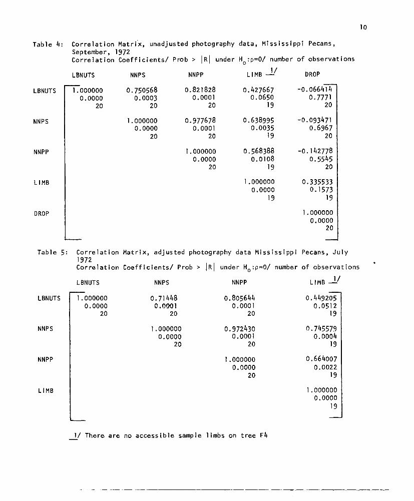
Table 4: Correlation Matrix, unadjusted photography data, Mississippi Pecans,Septembe r, 1972Correlation Coefficients/LBNUTS NNPS

LBNUTS 1.000000 0.7505680.0000 0.0003

20 20

NNPS 1.0000000.0000

20NNPP

LIMB

DROP

Prob > I RI under H :p=O/ number of observat ions0

NNPP LIMB _1/ DROP

0.821828 0.427667 -0.0664140.0001 0.0650 0.7771

20 19 20

0.977678 0.638995 -0.0934710.0001 0.0035 0.6967

20 19 20

1.000000 0.568388 -0. 1427780.0000 0.0108 0.5545

20 19 201.000000 0.335533

0.0000 o. 157319 19

1.0000000.0000

20

10

Table 5: Correlation Matrix, adjusted photography data Mississippi Pecans, July1972Correlation Coefficients/ Prob > IRJ under Ho:p=O/ number of observations

LBNUTS

NNPS

NNPP

LIMB

LBNUTS1.000000

0.000020

NNPS NNPP LIMB _1/

0.71448 0.805644 0.4492050.0001 0.0001 0.0512

20 20 19I.000000 0.972430 0.745579

0.0000 0.0001 0.000420 20 19

1.000000 0.6640070.0000 0.0022

20 191.000000

0.000019

1/ There are no accessible sample limbs on tree F4

II

Table 6: Correlation Matrix, adjusted photography data Mississippi Pecans, August1972Correlation Coefficientsl Prob > I RI under He :p=OI number of observations

I ILBNUTS NNPS NNPP LIM B -- DROP

LBNUTS 1.000000 0.899645 0.914822 0.439499 -0.0220930.0000 0.0001 0.0001 0.0571 0.9235

20 20 20 19 20NNPS I.000000 0.971275 0.462843 -0.057109

0.0000 0.0001 0.0438 0.805820 20 19 20

NNPP I.000000 0.332710 -0.0697740.0000 0.1611 0.7669

20 19 20

LIMB 1.000000 0.3927300.0000 0.0931

19 19DROP 1.000000

0.000020

Table 7: Correlation Matrix, adjusted photography data Mississippi Pecans,Sep tembe r 1972Correlation Coefficientsl Prob > IRI under He:p=OI number of observationsLBNUTS NNPS NNPP LIMB __II DROP

LBNUTS

NNPS

NNPP

LIMB

DROP

1.0000000.0000

20

0.,8469020.0001

20I.000000

0.000020

o 874279 0.427667 -0.0664140.0001 0.0650 0.7777

20 19 200.973825 0.538335 -0.108465

0.0001 0.0166 0.653020 19 201.000000 0.418659 -0.1634190.0000 0.0715 0.5024

20 19 201.000000 0.3355330.0000 o. 1573

19 191.000000

0.0000

__II There were no accessible sample limbs on tree F4

Analysis of Regression Models:Consider the linear regression model:

In the classical linear regression, Y is an observable random variable,

the X.'s are fixed observable variables, and the error term is an unob-I

served random disturbance. However, in our situation the regressor

variables are observable stochastic variables wbich are assumed to be

distributed independent of the disturbance. All the classical tests and

estimation procedures are valid when this assumption can be justified.

(Goldberger (3) discusses stochastic regression.)

In the analysis presented, the following models of the above form

were considered:

12

(M 1 )

(M2)

(M3)

(M4)(MS)(M6)(M7)

Y=Y=Y=Y=Y=Y=y=

+

+

+

+

+

+

+

(NNPS)

(NNPP)

(L 1MB)

(NNPS)(NNPP)

(NNPS)(NNPP)

+

+

+

+

(L 1MB)

(L1 MB)

(L 1MB)(LIMB)

+

+

(DROP)(DROP)

Y is the dependent variable LBNUTS. Note that M6 and M7 have more terms

than MI and M2 because of the inclusion of two independent variables.

The difference between MI and M2 (or between M4 and MS) is just the

different methods of expansion of the photography variable.Several questions arise about the models Ml through M7. Are all the

independent variables necessary in models M6 and M77 Which, if any, of

the seven models is the "best" regression model for forecasting average

weight of nuts per tree? These questions were considered and criteria

formulated to answer them.

Seven criteria will be proposed to answer the above questions. The

list of criteria is certainly not exhaustive but was chosen to evaluate

certain disirab1e properties. The criteria are as follows:

(CI) The square of the multiple correlation coefficient, R2• The

R2 value should increase by the inclusion of another pr possibly several

independent variables into the model. The larger the R2 value, the better

the model expl~ins the variation in the data. A substantial increase in

the R2 value for any model over Ml (or M2) by including the variable LIMBinto the regression would indicate that the LIMB variable is explaining

some additional variation in the data.

(C2) The standard error of estimate, s=1 s2 , the residual

mean square estimates the variance about regression cr2y·X. The smaller

the value of s the more precise will be the predictions.

13

The coefficent of variation, CV The CV = slY should decrease~

if increased precision is obtained by the inclusion of another variable.

(e4) The sequential F -test. This criterion accesses the contribution

of another variable added to an equation in stages. In (1) let SS(bo"" ,bk)be the sums of square due to regression.

Now for j=1,2, ... ,k let SS(bjlbo,b1 ... ,bj_1) be the sequential sums of

squares for the j-th beta parameter. SS(bjlbO,bl, ••• ,bj_l) is the difference

between the sums of squares due to the regression of Y on X1""'Xj and the

sums of square due to the regression of Y on Xl'" .,Xj_l. This is denotedby SS(bo,b, ,bj) and SS(bo,b" ... ,bj_l), respectively. The j-th sequential

F -test j=l ,2, k is:

F(b·lb ,... ,b. I) =J 0 J-

55 (b j I bo' , hj _I)

ESS (bo,b, ,bk)/N- (k+1)

14

ESS(bo,bl, ... ,bk) is the residual 55 of general model (I), and N is

the number of units in the sample. The above F has I and N-(k+l) de-

grees of freedom. Note that,

kL 55(bjlbo,.·.,bj_l) = 55(bo, ... ,bk).

j=l

Thus, the total sum of squares due to regression in the full model (I)is just partioned into single degrees of freedom 55's.

(CS) The partial F-test criteria. This criteria considers the orderin which the variables enter into the model. This criteria accesses the

value of a variable as if it were to enter the regression equation last.

The effect of Xj may be larger when the regression equation includes only

Xj. However, when the same variable entered into the equation afterother variables, it may affect the response very little. The F-test isas follows. For j=l, ... ,k

55 (bj I bo' b 1'... ,bj-1 'bj+ 1'... ,bk)=---------------ES5(bo,bl,··· ,bk)/N- (K+I)where,

55(bo,···,bj_l,bj+l,···,bk) is the sum of squares due to the regression of

Y on Xl,X2,···,Xj_l,Xj+I, ... ,Xk' i.e. the regression on all variables exceptthe j-th. This F has 1 and N-(k+l) degrees of freedom. It is not notedthat

has the T distribution with N-(k+l) d.f., and this statistic is used to

-------------------~~--- .._-~_._-~---~_._-----~------~------------

15

test if 13.=0 in (1). Thus, the j-th partial F-test is equivalent to aJ

T-test of 13·=0J .

(C6) The extra sums of square criteria. This criteria accesseswhether it was worth whi Ie to include certain terms in the general re-gression model (1). It is a joint test of the parameters 13j+l'... ,13kin (1). Consider the reduced model

(2) Y = 130+S1Xl+...+8qXqwhere q<k.And let SS(bo, ...b ) denotes the SS due to the regression (2).q

Then SS(bq+l, ..bklbo, ... ,bq)=SS(bo, ... ,bk)-SS(bo,bl, ...bq) is the extra

SS due to the inclusion of the terms Sq+1Xq+l+ ...+13kXk into the model(1). Now, the sum of squares SS(bo, .•. ,bk) has k d.f. and SS(bo"" ,bq)

has q d.f., thus SS(b l, ..• ,bklbo, ... ,b) has k-q d.f. So if e =8q+2= ...=8k=0q+ q q+lthen SS(bq+l, ... ,bklbo, ... ,bq) ~cr2X2 k-q, and is independnet of ESS(bo.b •...bk).

( I ) - _S S_(__bq••..•+-'-l_' _•• _. _' b__k__' ....;:bo"-,_·_.._,_b q•••.)_/_k -_q_Hence, F bq+ 1',...bk bo"'" b -q ESS(bo,bl····,bk)/N-(k+1)

has the F distribution with k-q and N-(k+l) d.f.

(C7) Significance of regression. This criteria determines whetherthe regression of Y on Xl •... ,Xk is significant. The test is

F =SS (b0' •.. , bk) /k

ESS (bo ,bl ,...bk) /N- (K+1)

This is a test of the hypothesis H:Sl=S2=",=Sk=O, 'which is equivalent to

testing that the true multiple correlation coefficient R is O.

The seven criteria can be broken into two general areas. First. the

R2, s, and CV are measures of how well the linear regression model fittedthe data. The other four criteria are statistical tests on certain para-

meters in the regression model. Tables 8 through 13 present the seven

- ....----- ..•..--.--- . ----------- ._--------------------

criteria to determine the "best" regression model. The analysis was done

using the STEPWISE procedure of the Statistical Analysis System (1).

This program deleted records with missing observations. Since tree F-4

has no accessible sample limbs it was deleted in the analysis presented.

16

Table 8: Criteria to determine the IIbestll regression model, adjusted photography data, Mississippi Pecans, July 1972

Criteria for IIbestll regression model

R2 Sequential F-test for Partial F-test for F forHODEL s C.V.% parameters 2/ oarameters ..Y slgnlfTcance of- II.B1 S2 S3-' : Sl 132 133 _1/ regression

HI 0.630 38.780 63.8 28. 97~': 28.97* 28.97*H2 0.741 32.486 53.5 48.52* 48. 53~': 48.52~':H3 0.202 56.977 93.8 4. 30~1:* 4 .30~:* 4.30~:*H4 0.676 37.414 61.6 31.13* 2.26 23.43~': 2.26 16.70~':M5 0.767 31.716 52.2 50. 90~': 1.84 38. 87~" 1.84 26.37*

** Indicates the F is significant a = .10* Indicates the F is significant a = .011/ Drop was not observed the first month

:2/ A blank indicates that the F test isnot app 1icafij-}ewith th is mode 1.

Table 9: Criteria to determine the "best" regression model, adjusted photography data, Missisippi Pecans, August1972

Criteria for "best" reg ress ion modelSequential F-test for Partial F-test for :F-test for extra F for:MODEL R2 s C.V.% parameter 1/ parameter 1/ SS Criteria :significance of81 82 83 81 82 83 :models M6 and M7 regressionHo :82"83 =0

Ml 0.901 20.089 33. 1 154.32'~ 154.32* 154.32'~M2 0.869 23.065 38.0 112.96* 112.96'~ 112.96,1,M3 o. 193 57.284 94.3 4.07:~* 4.07* 4 .07:~*M4 0.901 20.707 34. 1 145 .25:~ 0.00 114. 1O'~ 0.00 72. 62'~M5 0.888 21.999 36.2 124.17* 2.68 99. 26:~ ].68 68.43'~M6 0.904 20.997 34.6 141.27* 0.44 0.12 105 .85:~ 0.56 0.12 0.281 47.28:~M7 0.888 22. 720 37.4 116.42:" 2.52 0.00 88.21* 2.09 0.00 1.26 39.65'"

** Indicates the F is significant a •. 10* Indicates the F is significant a = .011/ A blank indicates that the F-test is not applicable wfth this model.

00

Table 10: Criteria to determine the "best" regression model, adjusted photography, Mississippi Pecans, September 1972

Criteria for "best" regress ion modelSequential F-test for Partial F-test :F-test for extra: F forSS Cri teri a :

MODEL R2 s C.V.% parameter 1/ parameter _1/ :mode 15 M6 and M7: significance ofregression131 132 133 81 82 83 H :132=133=00

Ml 0.818 27.200 44.8 76.45* 76.45* 76.45''<

M2 0.812 27.655 45.5 73.4P 73.41* 73.45''<

M3 0.183 57.647 94.9 8.81 *,,< 3.81*''< 3.81*":

M4 0.823 27.653 45.5 73.96* 0.45 57.87* 0.44 37.20":

M5 0.815 28.271 46.5 70.24* 0.27 54.68''< 0.27 35.26''<M6 0.846 26.683 43.9 79.45''< 0.94 1.73 61.75''< 2.19 1.73 1.33 27.371":M7 0.829 28.050 46.2 71.35''< 1.52 0.00 54.45''< 1.25 0.00 0.76 24.28''<

** "Indicates the F is significant~ a = .10* Indicates the F is significant. a = .011/ A blank indicates that the F-test is not applicable with this model.

Table II: Criteria to determine the "best" regression model, unadjusted photography Mississippi Pecans, July 1972

Criteria for "best" regression modelSequential F-teSj for Partial F-test for

pa ramete r ...l oarameter 21 F forR2 - significanceMODEL s C.V.% II: 83 _II81 82 83 -. 81 82 of regression

Ml 0.421 48.527 79.9 12.36* 12.36* 12.36*

M2 0.518 44.258 72.9 18.30* 18.30* 18.30*

M3 0.202 56.977 93.8 4.30** 4.30** 4.30**

M4 0.462 48.235 79.4 12..51* 1.20 7.72** 1.21 6.86*

M5 0.575 42.878 70.6 19.49* 2.11 14.02* 2. II 10.80*

** Indicates the F is significant a = .10* Indicates the F is significant a = .01II Drop was not observed the first visit

21 A blank indicates that the F-test is not applicable with this model.

No

Table 12: Criteria to determine the "best" regression model, unadjusted photography data, Mississippi Pecans,August1972

Cri teria for "best" regression modelSequential F-f7st for: Partial F-tes1 for :F-test for extra:

R2 parameter __ : parameter _1 : 55 Criteria F forMODEL s C.V.% :models M6 and M7: significance

81 82 8s 81 82 8s H :e2=8 3=0 of regression0

Ml 0.793 29.041 47.8 64.98* 64.98* 64. 98,~

M2 0.874 22.663 37.3 117.62* 117.62* 117.62*

M3 0.193 57.284 94.3 4.07H 4.07*'~ 4.07*

M4 0.799 29.496 48.6 62.99'~ 0.48 48. 12'~ 0.48 31 .73'~

M5 0.874 23.358 38.5 110.71* 0.00 86 ..24* 0.00 55.36*

M6 0.806 29.906 49.2 61.27* 0.47 0.56 44.56* 0.94 0.56 0.546 20. 77*

M7 0.876 23.894 39.3 105.81* 0.20 0.09 78.32* 0.29 0.09 0.147 35.37*

** Indicates the F is significant a = .10* Indicates the F is significant a = .01l/A blank indicates that the F-test is not applicable with this model.

N

Table 13: Criteria to determine the "best" regression model, unadjusted photography, Mississippi Pecans, September1972

Criteria for Ilbest" regression modelSequential F-test for Partial F-tesf for :F-test for extra: F forparameter 1/ parameter / SS Crite riaR2 C.V.% - significanceMODEL s :models M6 and M7: of regression

81 82 83 81 82 8 3 Ho :82= 8 3"'0

MI 0.668 36.724 60.5 34. 27'~ 34.27'~ 34. 27'~

M2 0.749 31.915 52.6 50.88* 50.88* 50 .88,~•• _~'l

M3 o. 183 57.647 94.9 3 .81,~,~ 3.81** 3.81*M4 0.688 36.978 60.9 33.80* 0.77 25. 32'~ 0.77 17 .28'~

M5 0.756 32.492 53.5 49.09* 0.40 37.51"< 0.40 24.741<

M6 0.714 36.328 59.8 35 .02'~ 0.79 1.58 26.40* 2.02 1.58 1. 19 I2 .46'~

M7 0.790 31.114 51.2 53.53* 1.00 1.88 41 .44'~ 2.45 1.88 1.41, 18.81)~

** Indicates the F is sifnificant a = .10* Indicates the F is significant a = .011/ A blank indicates that the F-test is not applicable under this particular model.

NN

DISCUSSION OF RESULTS

Inspecting the correlation matrices (Tables 2-7) indicate that most

of the variables are correlated with yield (LBNUTS). However, DROP is not

significantly correlated with yield for any month, nor was DROP signifi-

cantly correlated with any of the other independent variables. This con-

firms earlier findings of WooB (7,P·,15;6,p.12).

However, DROP was included in all the regression analysis presented

since even if the correlation between two variables is small it may in-.

fluence the multiple correlation coefficient (r) a great deal when several

variables are in a regression model simultaneously. In this particular

case, it was not true that DROP had a substantial effect on the coefficient

of determination, which is the square of the multiple correlation coefficient.

This can be seen by comparing Models M4 and M6 and Models M5 and M7 in Tables

8 through 13. Based on these findings and previous results (by Wood (6,7))

drop counts should not be included in any further work in developing

a pecan forecast model.There also appears to be a stronger relationship between final

harvested weight of nuts with adjusted photography variates, than with

the unadjusted photography. This indicates that interpreter adjustment

factors are necessary. The sample correlation coefficient of the photo

variable with LBNUTS is always greater than the limb count variable LIMB.

Also, in general, the photo count variable NNPP has larger sample correlation

coefficient than does the photo count variable NNPS. This could possibly

be attributed to a more precise estimate of the bearing surface of a treeby assuming the tree is a parabolid rather than a sphere.

Tables 8 through 13 show that:

23

1. Each regression is significant at the .01 level.

2. The F-test is the extra SS criteria (where applicable) is in-

significant. Thus, 82 and 83 are simultaneously zero in Models

M6 and M7.2. The partial F-test indicates that the LIMB and DROP variables

contributed very little when they were included in the last

stage. However, the contribution of the photo count variables

is important even when the LIMB and/or DROP variables are in-•troduced in the equation first. This is indicated by the sig-

nificant Partia1-F of the 81 parameter.

4. Once the photo variable was in the model the contribution ofadditona1 variables were significant. This is indicated by the

sequential F-test.

5. Comparing Models M1 through M3 indicates that in each case M1

and M2 have larger R2·s and smaller standard errors than Model

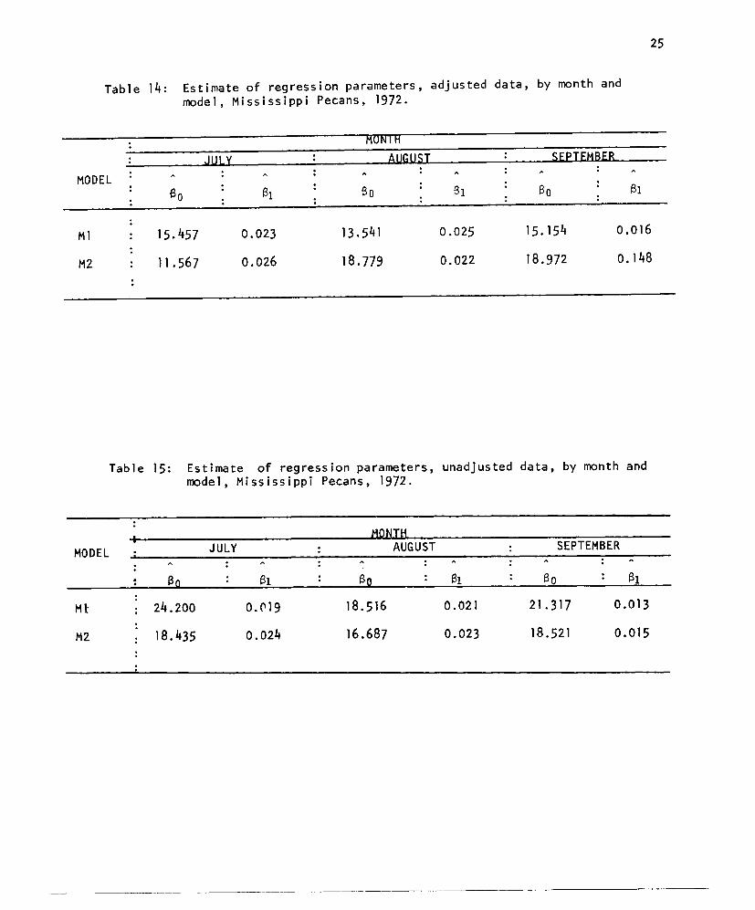
M3.What the seven criteria indicate is that only one variable needs

to be considered (and collected); it is the photographic variable. Fur-

ther, M1 or M2 is the "best" regression model to use to forecast yield

per tree. Table 14 and 15 give the estimated regression parameters

for Models M1 and M2. When fitting these models, plots of residuals

were examined for any departure from any of the underlying assumptions.

(Draper and Smith (2) describe methods for examining residuals.) None

was found.

24

25

Table 14: Estimate of regression parameters, adjusted data, by month andmodel, Mississippi Pecans, 1972.

MODEL

Ml

M2

MONIH

JULY AUGUST SEPTEMBER

eo 81 80 81 80 81

15.457 0.023 13.541 0.025 15.154 0.016

11.567 0.026 18.779 0.022 18.972 0.148

Table 15: Estimate of regression parameters, unadjusted data, by month andmodel, Mississippi Pecans, 1972.

MONTHMODEL JULY AUGUST SEPTEMBER

ao 81 80 81 80 81

Ml 24.200 0.019 18.516 0.021 21.317 0.013

M2 18.435 0.024 16.687 0.023 18.521 0.015

--~"~_._~-----------------~ ------------- --------- ----------------

26

CONCLUSIONS

Based upon the analysis performed on data collected in 1972, only

photographs need to be collected in any further pecan research for fore-

casting yield per tree (LBNUTS) until improvements in the limb sampling

procedure can be achieved which will make the accessible limbs representa-

tive of a larger portion of the tree. This will require the use of a

type of mechanical lift equipment which was not available for this study.

The variable DROP failed to be significantly correlated with yield nor

was it useful in model building. The variable LIMB is not needed in anyforecasting model once any type of photographic variable is in the model.

RECOMMENDATIONS

Future research studies should focus attention on photographic data

collection and improving this technique for this particular nut crop.

Different expansions to a tree level using photography may produce

even better results. A more refined estimate of the height may also

improve the expansions on a per tree basis. However, other characteristics

of the tree and its immediate environment must not be overlooked. For

example, how do differing management techniques influence yield? Possibly

this answer is Ilgreatly", indicating that stratification based on management

practices might be necessary.

A random selection of blocks of different varieties and ages is needed to

determine if different forecast models are needed. This will necessitate a

complete sampling frame of operations for the population. Accurate estimates of

tree numbers by individual blocks must be secured for each operation.

Future investigation should also consider whether monthly models

.~------------------~-_._------~----------~----~-------------

27

are necessary for forecasting yield per tree. Possibly the regression

parameters would be stable over months during the growing season indicating

that just the development and maintenance of only one forecasting equation

would be necessary. Thus, monthly change in average yield per tree would

be reflected in the change in average photo counts per tree and not in the

change in beta parameters.The under-estimation of total number of nuts counted on photographs

needs further analysis and investigation. If the magnitude of under-esti-

mation is consistent year-to-year, the use of a relative change forecast

of production could be utilized based on either photo counts or accessible

limb counts. This method of estimation is used in Florida on citrus. For

example, an estimation of the following form for a particular variety and

age class might bex x P , where

t-l

P is the forecast of productton in year t,t

Pt-l is the actual production for the previous year,

Nt is the forecasted average weight (or number) of nuts per tree

using the photo expansion for year t,

Nt-l is the average weight (or number) of nuts per tree using the

photo expansion for year t-l,

Tt is the number of bearing trees of a particular age and variety

for year t,

T is the number of bearing trees of a particular age and varietyt-l

for year t-l.Another ratio (Ht/Ht_l) could be included in (1) to indicate the

proportion of nuts intended for commercial harvest. This ratio would

28

probably be very volatile since price and the tendency of the trees to be

cyclic in yield usually determine whether a noncommercial operator will

harvest his pecan crop.It should be noted that for this forecast the actual production is

needed for a particular region by variety and age of trees. Also, accurate

estimates of the relative change in number of. bearing trees must be secured.

Observe also that Nt/Nt_1 is the relative change in estimated weight of nuts

per tree, so that if the method of expansion and estimation consistently

under-estimates the true weight of nuts per tree, this effect will cancel

out in the ratio. A more detailed discussion of this forecast method

can be found in Stout (5) and Williams (6).

Finally, counting the nuts on slides is tedius difficult, and very

time consuming. Automated fruit counting procedures would be extremely

desirable for any operational level study.

m __ ._~~ ~. . _

REFERENCES

1. Barr, Anthony J., and Goodnight, James H., "A User's Guide to the

Statistical Analysis System", Raleigh: Student Store, North Carolina

State University, 1971.

2. Draper, Norman and Smith, Harry, IIApplied Regression Analysis", New

York: John Wiley and Sons, 1966.

3. Goldberger, Arthur S., "Econometric Theory", New York: John Wiley

and Sons, 1964.

4. Huddleston, Harold F., liThe Use of Photography in Sampling for Number

of Fruit Per Tree", Agriculture Economic Research, July 1971, Vol. 23,

No.3.5. Stout, Roy G., "Estimating Citrus Production by Use of Frame Count

Surveyl', Journal of Farm Economics, November 1962, Vol. XLIV, No.4.

pp.1037-1049.6. William, S. R., "Forecastihg Florida Citrus Production Methodology &

Development", January 1971, "Florida Crop and Livestock Reporting

Service", Orlando, Florida.

7. Wood, Ronald A., "A study of the Characteristics of the Pecan Tree for

Use in Objective Yield Forecasting", Research and Development Branch,

Standards and Research Division. Statistical Reporting Service, U.S.

Department of Agriculture, Washington, D.C.

8. Wood, Ronald A., liThe Development of Objective Procedures to Estimate

Yield for Pecan Treesl', Research and Development Branch, Research Divi-

sion, Statistical Reporting Service, U. S. Department of Agriculture,

Washington, D.C.

29