ReviewAutomatic Control

Instructor: Cailian Chen, Associate ProfessorDepartment of Automation

27 December 2012

23/4/19 2

Structure of the courseLinear Time-invariant System (LTI)

各章概念融会贯通解题方法灵活运用

Concepts System Model

PerformanceTime DomainComplex DomainFrequency Domain

Analysis

Compensation Design

23/4/19 3

1 2

1 2

1 1

2

1 1

2

]12)[()1(

]12)[()1(

)(

)(n

j

n

l pnpnj

m

i

m

k znkznki

ll

ssss

sssK

sR

sC

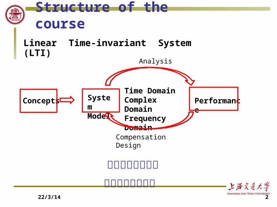
Time Constant Canonical Form (Bode Form)

；

； Root Locus Canonical Form (Evan’s Form)

1 2

1 2

( )( ) ( )( )( )

( ) ( )( ) ( )r m

n n

K s z s z s zN sG s

D s a s p s p s p

LL

23/4/19 4

j

0

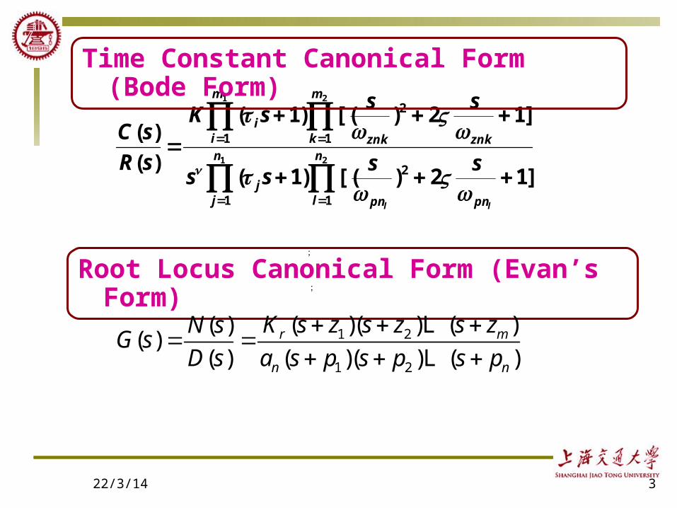
Stable RegionUnstable Region

[S plane]

(1) Routh Formula (2) Root Locus Method (3) Nyquist Stability Criterion

Stability Analysis Method

Stability: All of the roots of characteristic equation of the closed-loop system locate on the left-hand half side of s plane.

Z ＝ N ＋ P

23/4/19 5

Understand and remember of root locus equation

Rules for sketching of root locus Calculate Kg and K by using magnitude

equation

Summary of Chapter 5

23/4/19 623/4/19 6

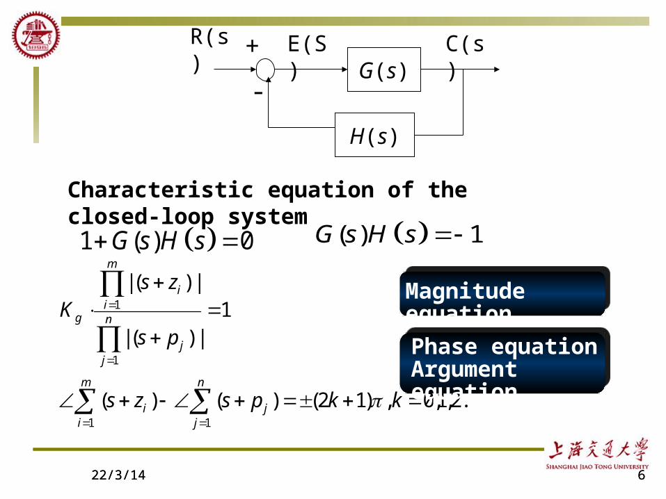
Characteristic equation of the closed-loop system

1 ( ) 0G s H s ( ) 1G s H s

R(s)

G(s)

H(s)

+

-

C(s)E(S)

...2,1,0,)12()()(

1|)(|

|)(|

11

1

1

kkpszs

ps

zsK

n

jj

m

ii

n

jj

m

ii

g

Phase equationArgument equation

Magnitude equation

7

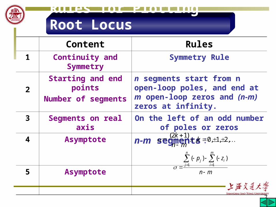
Content Rules1 Continuity and Symmetry Symmetry Rule

2

Starting and end points

Number of segments

n segments start from n open-loop poles, and end at m open-loop zeros and (n-m) zeros at infinity.

3 Segments on real axis On the left of an odd number of poles or zeros

4 Asymptote n-m segments ：

5 Asymptote

mn

zpn

j

m

iij

1 1

)()(

,2,1,0,)12(

kmn

k ＝

Rules for Plotting Root Locus

8

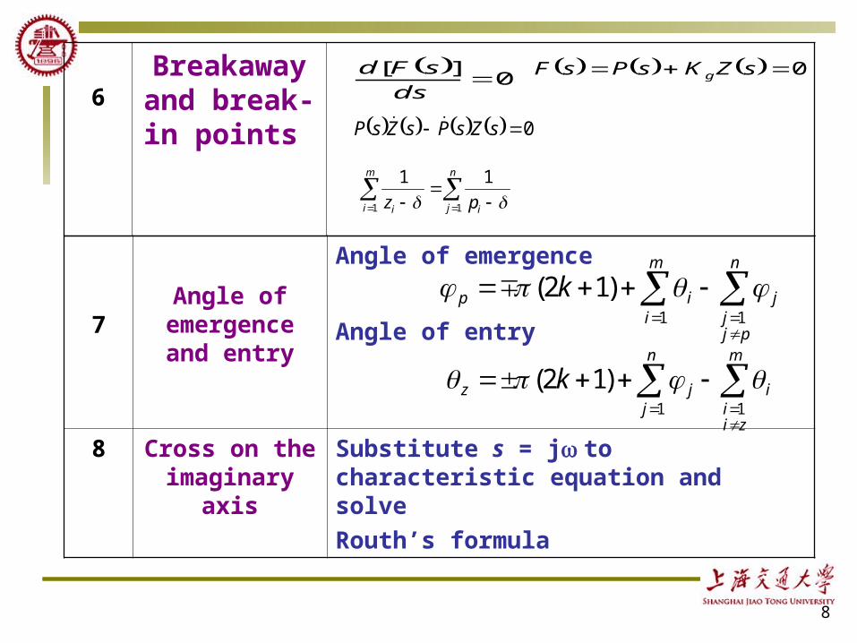
7Angle of

emergence and entry

Angle of emergence

Angle of entry

8 Cross on the imaginary axis

Substitute s = j to characteristic equation and solve

Routh’s formula

n

j

m

zii

ijz k1 1

)12(

m

i

n

pjj

jip k1 1

)12(

6Breakaway

and break-in points

0

][

ds

sFd 0 sZKsPsF g

0 sZsPsZsP

m

i

n

j ii pz1 1

11

23/4/19 923/4/19 9

180 (2 1)( 0,1,2, )

kk

n m

1 1

n m

j ij i

p z

n m

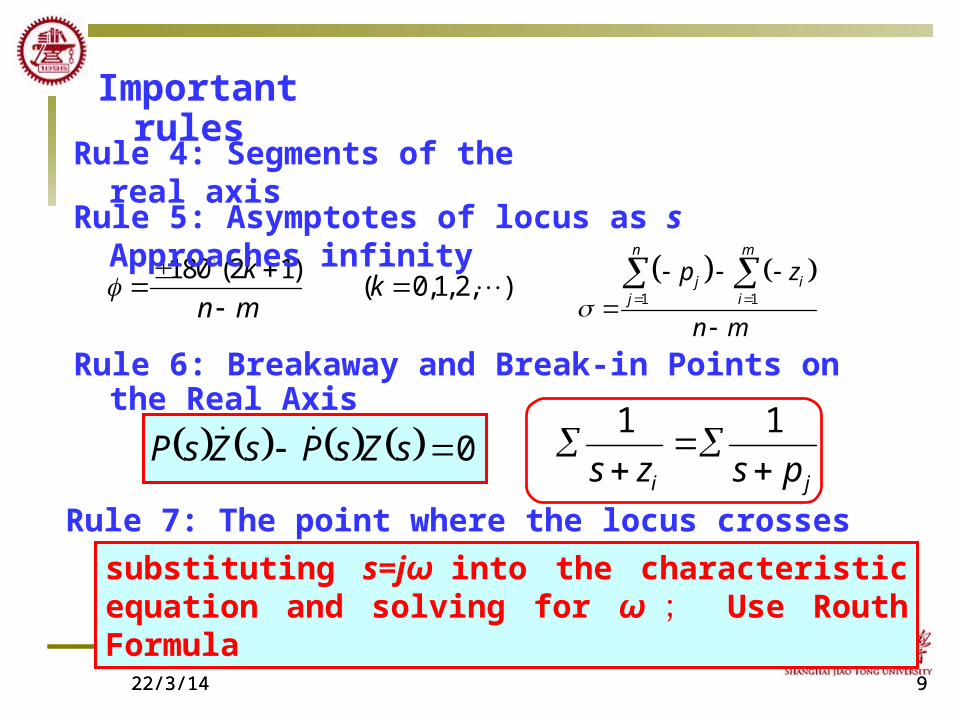
Important rules

Rule 4: Segments of the real axis

Rule 5: Asymptotes of locus as s Approaches infinity

Rule 6: Breakaway and Break-in Points on the Real Axis

0 sZsPsZsP ji pszs

11

Rule 7: The point where the locus crosses the imaginary axis

substituting s=jω into the characteristic equation and solving for ω ； Use Routh Formula

23/4/19 10

Summary of Chapter 6

Complete Nyquist Diagram Bode Diagram Nyquist Stability Criterion Relative Stability

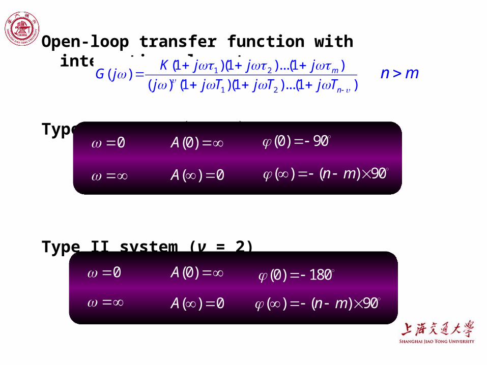
Open-loop transfer function with integration elements

Type I system （ ν ＝ 1 ）

Type II system (ν = 2)

0

(0)A (0) 90

( ) 0A ( ) ( ) 90n m

1 2

1 2

(1 )(1 )...(1 )( )

( ) (1 )(1 )...(1 )m

n

K j j jG j

j j T j T j T

n m

0

(0)A (0) 180

( ) 0A ( ) ( ) 90n m

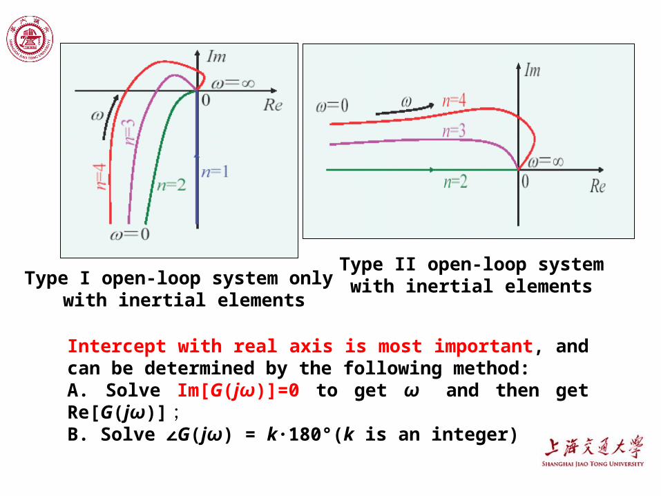
Type I open-loop system only with inertial elements

Type II open-loop systemwith inertial elements

Intercept with real axis is most important, and can be determined by the following method:A. Solve Im[G(jω)]=0 to get ω and then get Re[G(jω)] ；B. Solve ∠G(jω) = k·180°(k is an integer)

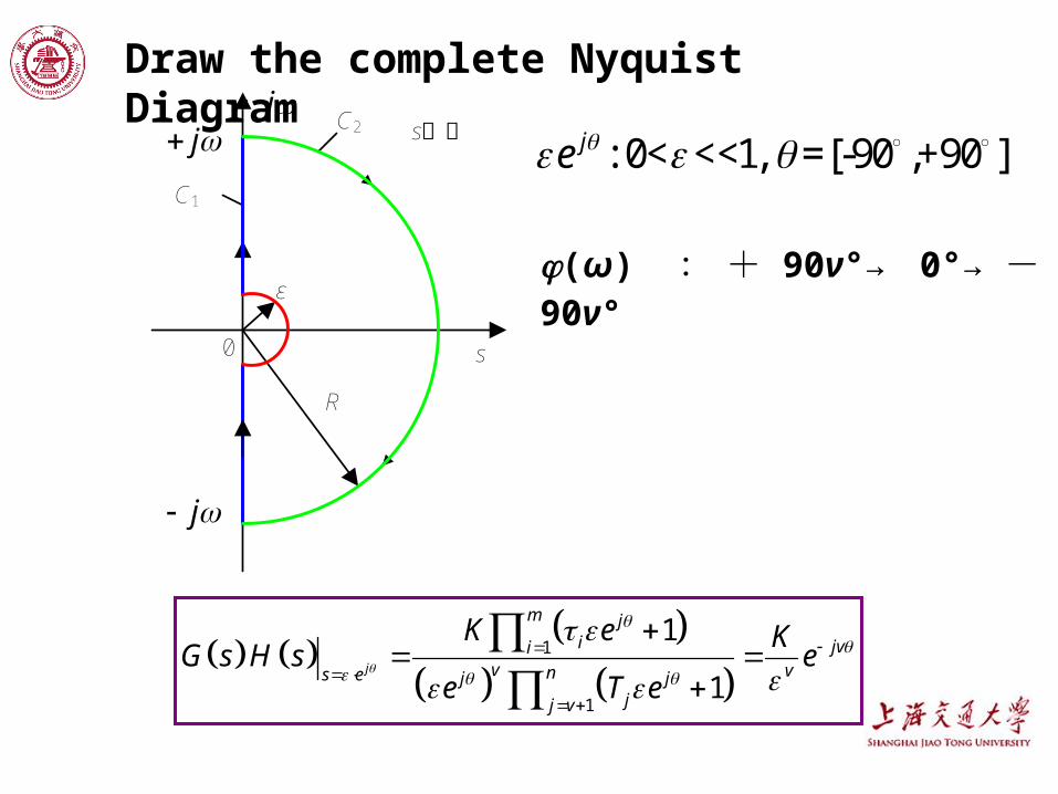
0 s

s平面

ε

C1

C2

R

jj

j

(ω) ：＋ 90ν°→ 0°→ － 90ν°

: 0< <<1, =[-90 ,+90 ]je

1

1

1

1j

m ji jvi

v vns e j jjj v

K e KG s H s e

e T e

Draw the complete Nyquist Diagram

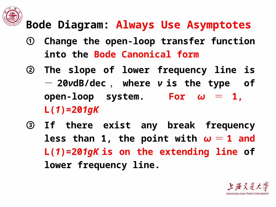
Bode Diagram: Always Use Asymptotes

① Change the open-loop transfer function into the Bode

Canonical form

② The slope of lower frequency line is

－ 20νdB/dec ， where ν is the type of open-loop

system. For ω ＝ 1, L(1)=201gK

③ If there exist any break frequency less than 1, the

point with ω ＝ 1 and L(1)=201gK is on the extending

line of lower frequency line.

Nyquist stability criterion

• If N≠ － P ， the closed-loop system is unstable.

The number of poles in the right-hand half s plane

of closed-loop system is Z ＝ N ＋ P.

• If the open-loop system is stable ， i.e. P=0 ， then

the condition for the stability of closed-loop system

is: the complete Nyquist diagram does not encircle

the point

( － 1, j0), i.e. N=0.

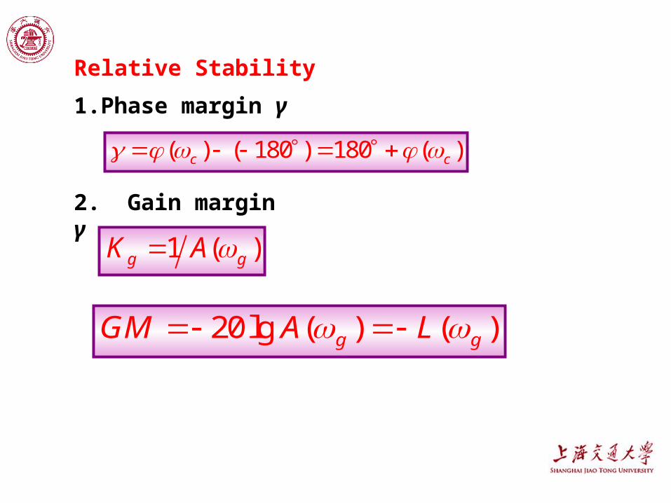
Relative Stability

1. Phase margin γ

( ) ( 180 ) 180 ( )c c

1 ( )g gK A

20lg ( ) ( )g gGM A L

2. Gain margin γ

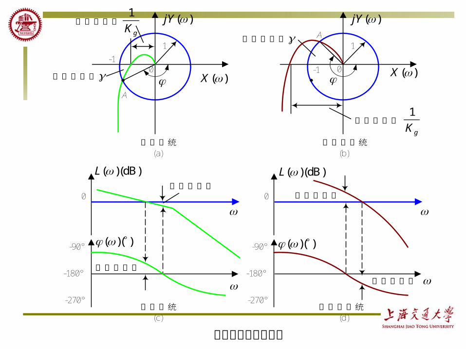
相角裕度和增益裕度

0

-90°

-180°

-270°

0

-90°

-180°

-270°稳定系统

(c)

正相角裕度

正增益裕度

负增益裕度

负相角裕度

不稳定系统(d)

0

A

正相角裕度

-1

1

0

A

-1

1

稳定系统(a)

不稳定系统(b)

负增益裕度

负相角裕度

正增益裕度

( )(dB)L

( )( )

( )(dB)L

( )( )

( )jY

( )X

( )jY

( )X

1

gK

1

gK

23/4/19 1823/4/19 18

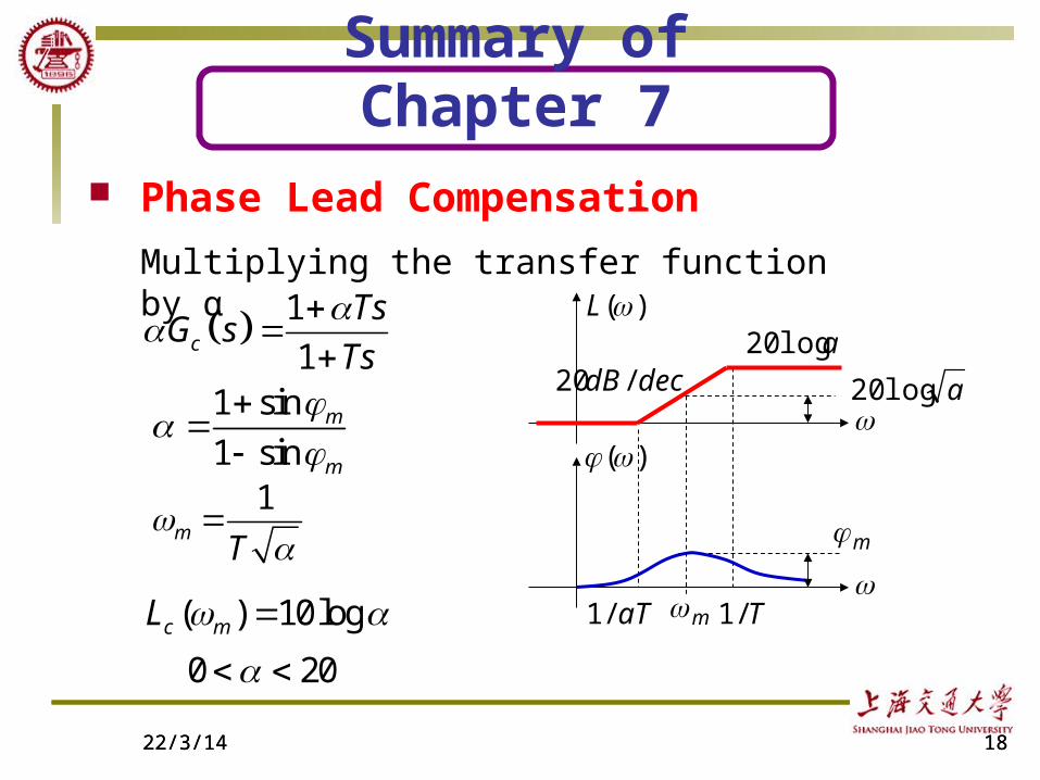
Phase Lead Compensation

Summary of Chapter 7

1m

T

)(L

decdB /20

alog20

alog20

aT/1 m

)(

T/1

m

( ) 10logc mL

0 20

Multiplying the transfer function by α

1 sin

1 sinm

m

1

1c

TsG s

Ts

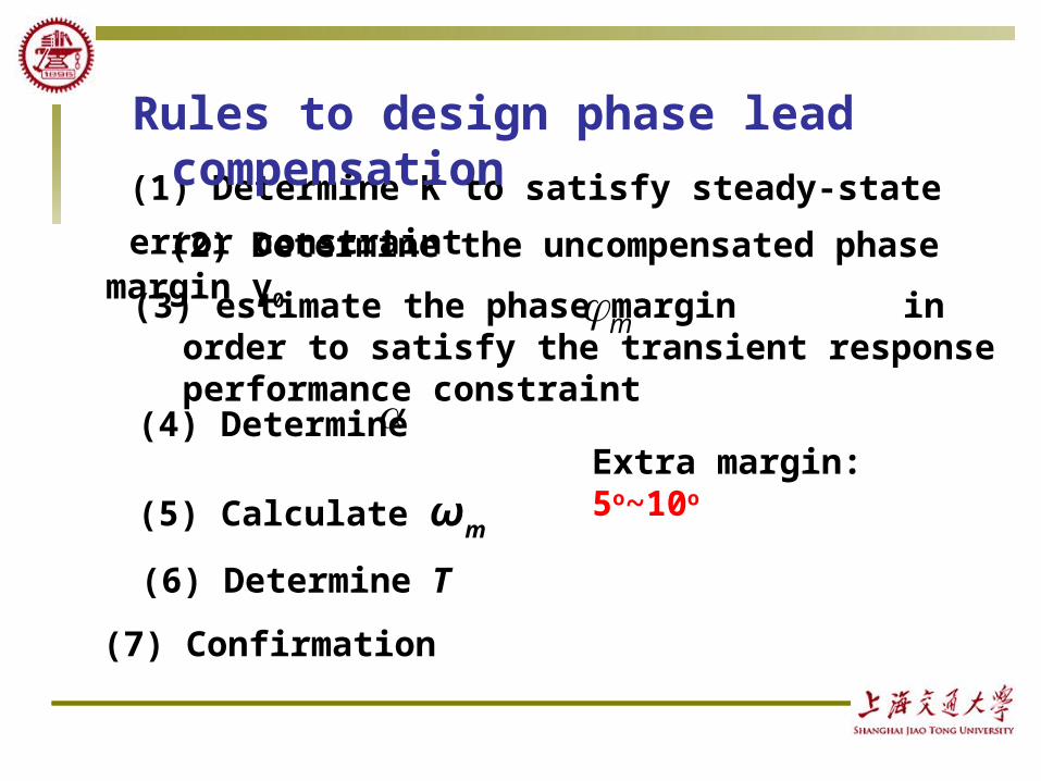
(4) Determine

(2) Determine the uncompensated phase margin γ0

(7) Confirmation

(1) Determine K to satisfy steady-state error

constraint

(5) Calculate ωm

(6) Determine T

(3) estimate the phase margin in order to satisfy the transient response performance constraint

Rules to design phase lead compensation

m

Extra margin:5o~10o