Embed Size (px)
Citation preview
Scalar and Vector Quantization
National Chiao Tung University
Chun-Jen Tsai
11/06/2014
2/55
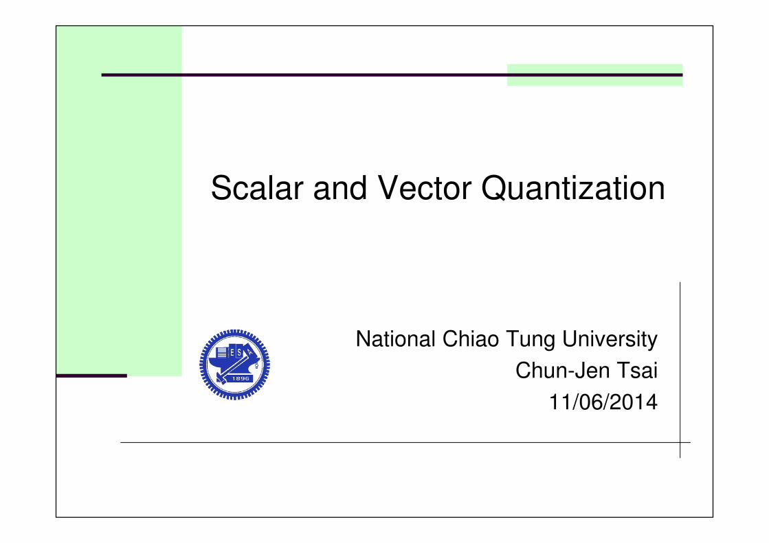
Basic Concept of Quantization
� Quantization is the process of representing a large,
possibly infinite, set of values with a smaller set
� Example: real-to-integer conversion
� Source: real numbers in the range [–10.0, 10.0]
� Quantizer: Q(x) = x + 0.5
� [–10.0, –10.0] → { –10, –9, …, –1, 0, 1, 2, …, 9, 10}
� The set of inputs and outputs of a quantizer can be
scalars (scalar quantizer) or vectors (vector quantizer)
3/55
The Quantization Problem
� Encoder mapping� Map a range of values to a codeword
� Irreversible mapping
� If source is analog → A/D converter
� Decoder mapping� Map the codeword to a (fixed) value representing the range
� Knowledge of the source distribution can help us pick a better value representing each range
� If output is analog → D/A converter
� Informally, the encoder mapping is called the quantization process, and the decoder mapping is called the inverse quantization process
4/55
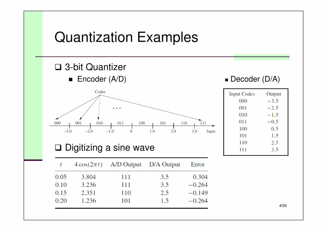
Quantization Examples
� 3-bit Quantizer
� Encoder (A/D) � Decoder (D/A)
� Digitizing a sine wave
5/55
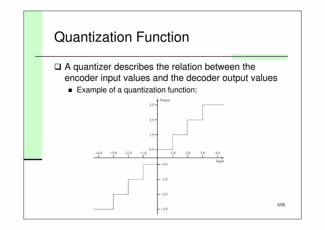
Quantization Function
� A quantizer describes the relation between the
encoder input values and the decoder output values
� Example of a quantization function:
6/55
Quantization Problem Formulation
� Input:
� X – random variable
� fX(x) – probability density function (pdf)
� Output:
� {bi}i = 0..M decision boundaries
� {yi}i = 1..M reconstruction levels
� Discrete processes are often approximated by
continuous distributions
� Example: Laplacian model of pixel differences
� If source is unbounded, then the first and the last decisionboundaries = ±∞ (they are often called “saturation” values)
7/55
Quantization Error
� If the quantization operation is denoted by Q(·), then
Q(x) = yi iff bi–1 < x ≤ bi.
The mean squared quantization error (MSQE) is then
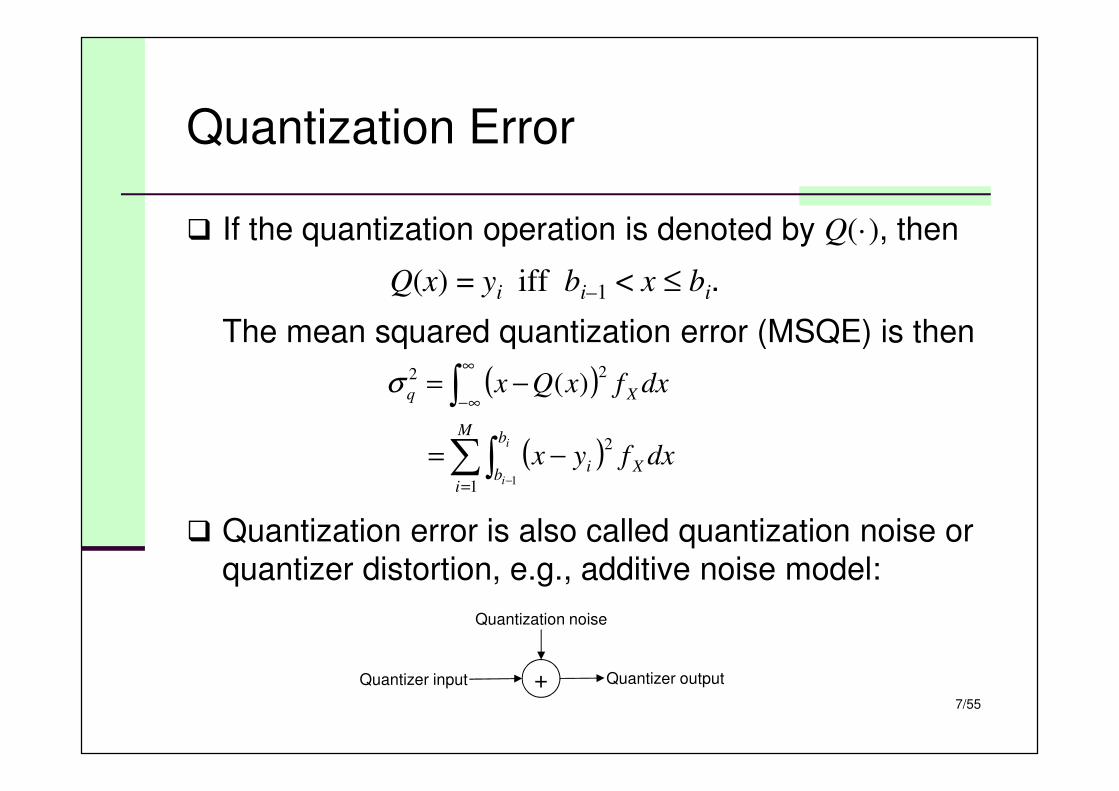
� Quantization error is also called quantization noise or
quantizer distortion, e.g., additive noise model:
( )
( )∑∫
∫
=
∞
∞−
−
−=
−=
M
i
b
bXi
Xq
i
i
dxfyx
dxfxQx
1
2
22
1
)(σ
+Quantizer input
Quantization noise
Quantizer output
8/55
Quantized Bitrate with FLC
� If the number of quantizer output is M, then the rate
(per symbol) of the quantizer output isR = log2M� Example: M = 8 → R = 3
� Quantizer design problem:
� Given an input pdf fX(x) and the number of levels M in the quantizer, find the decision boundaries {bi} and the reconstruction levels {yi} so as to minimize the mean
squared quantization error
9/55
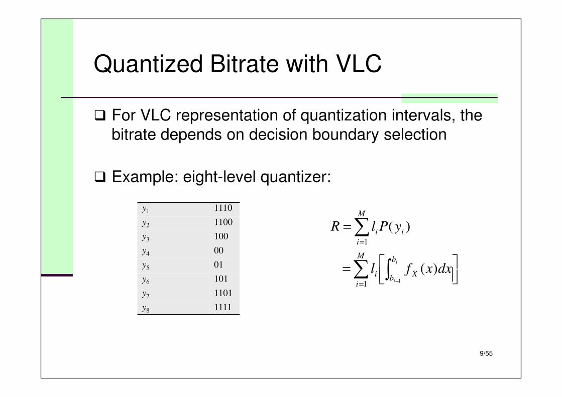
Quantized Bitrate with VLC
� For VLC representation of quantization intervals, the
bitrate depends on decision boundary selection
� Example: eight-level quantizer:
∑ ∫
∑
=
=
=
=
−
M
i
b
bXi
M
i
ii
i
i
dxxfl
yPlR
1
1
1
)(
)(
y1 1110
y2 1100
y3 100
y4 00
y5 01
y6 101
y7 1101
y8 1111
10/55
Optimization of Quantization
� Rate-optimized quantization
� Given: Distortion constraint σq2 ≤ D*
� Find: { bi }, { yi } binary codes
� Such that: R is minimized
� Distortion-optimized quantization
� Given: Rate constraint R ≤ R*
� Find: { bi }, { yi } binary codes
� Such that: σq2 is minimized
11/55
Uniform Quantizer
� All intervals are of the same size
� Boundaries are evenly spaced (step size:∆), except for out-most intervals
� Reconstruction
� Usually the midpoint is selected as the representing value
� Quantizer types:
� Midrise quantizer: zero is not an output level
� Midtread quantizer: zero is an output level
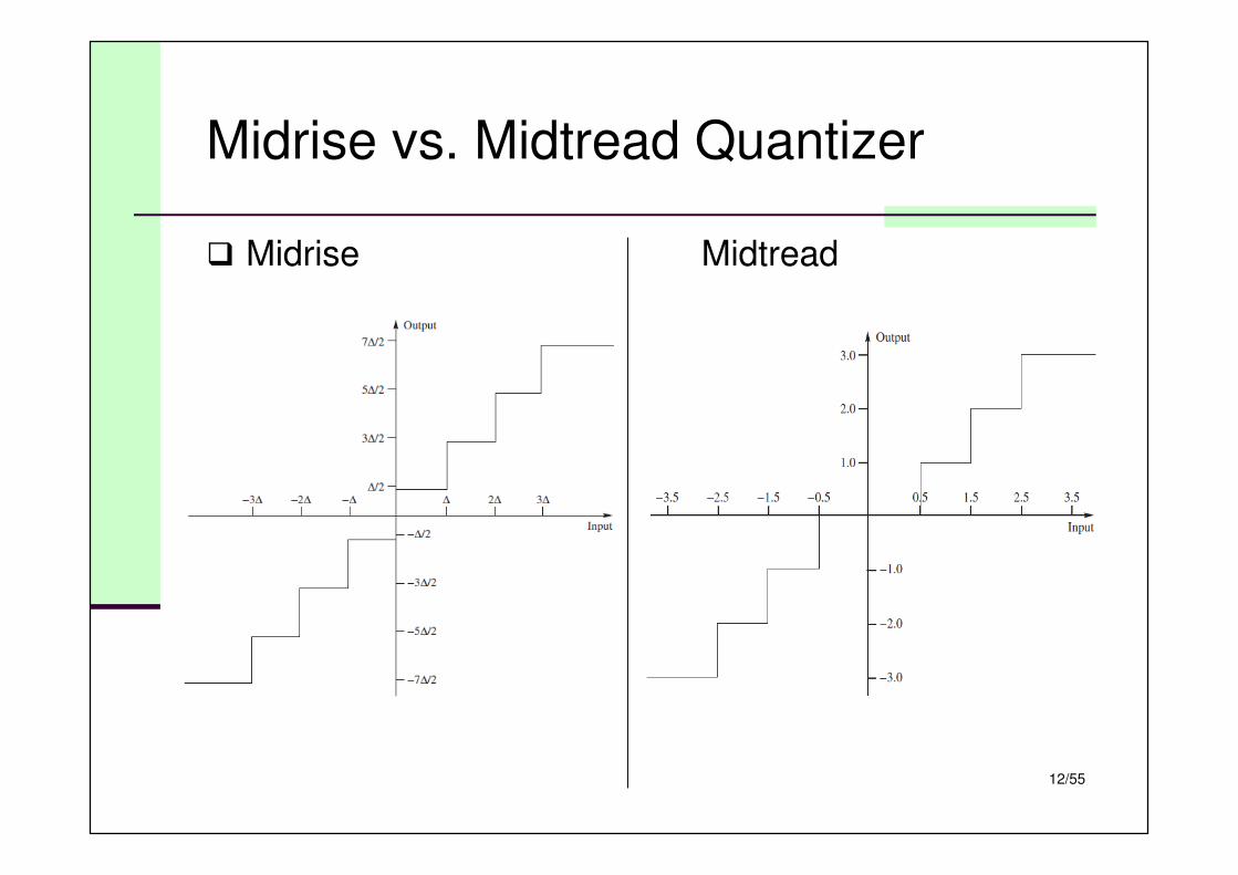
12/55
Midrise vs. Midtread Quantizer
� Midrise Midtread
13/55
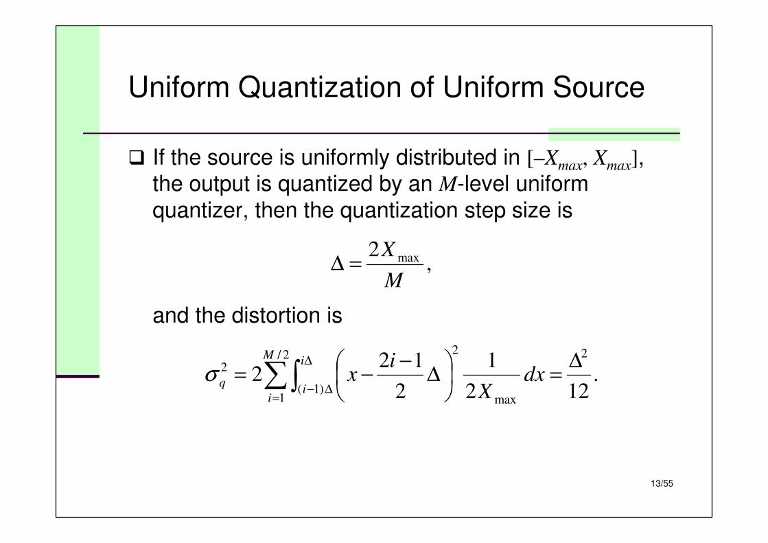
Uniform Quantization of Uniform Source
� If the source is uniformly distributed in [–Xmax, Xmax],
the output is quantized by an M-level uniform
quantizer, then the quantization step size is
and the distortion is
,2 max
M
X=∆
.122
1
2
122
22/
1)1(
max
2
2 ∆=
∆
−−= ∑∫
=
∆
∆−
M
i
i
iq dx
X
ixσ
14/55
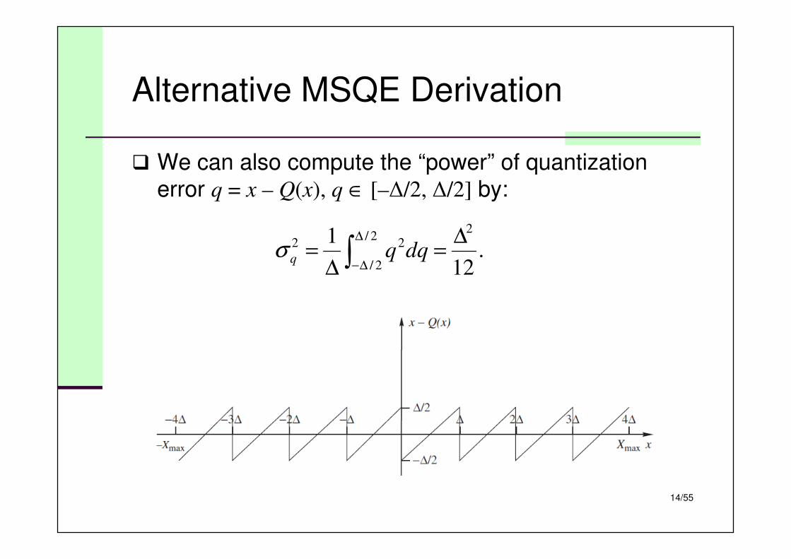
Alternative MSQE Derivation
� We can also compute the “power” of quantization error q = x – Q(x), q ∈ [–∆/2, ∆/2] by:
.12
1 22/
2/
22 ∆=
∆= ∫
∆
∆−dqqqσ
15/55
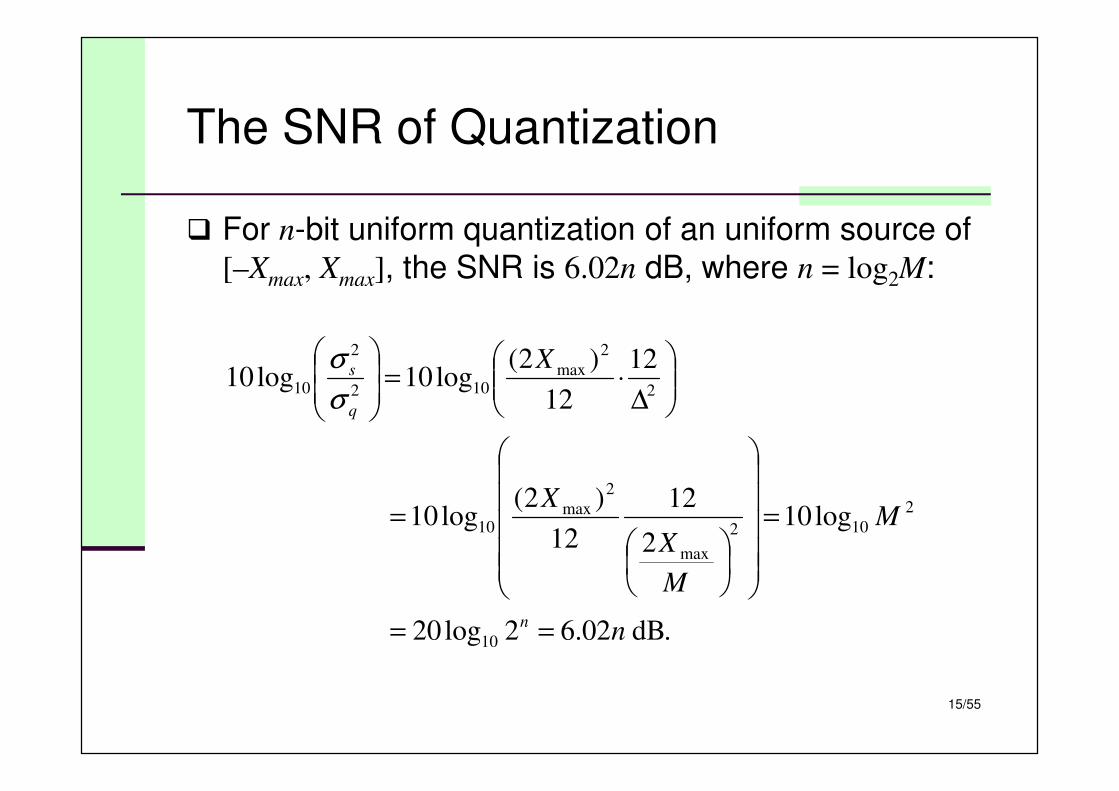
The SNR of Quantization
� For n-bit uniform quantization of an uniform source of
[–Xmax, Xmax], the SNR is 6.02n dB, where n = log2M:
.dB02.62log20
log102
12
12
)2(log10
12
12
)2(log10log10
10
2
102
max
2
max10
2
2
max102
2
10
n
M
M
X
X
X
n
q
s
==
=
=
∆⋅=
σ
σ
16/55
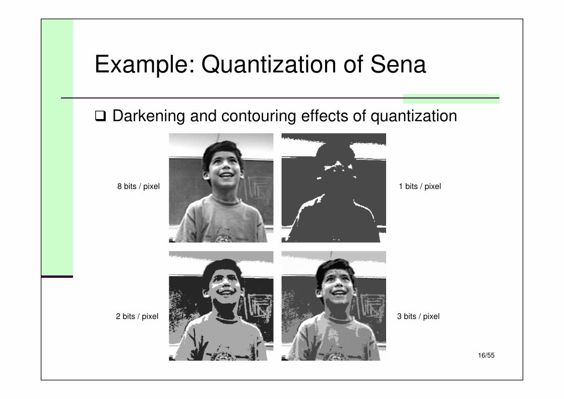
Example: Quantization of Sena
� Darkening and contouring effects of quantization
8 bits / pixel
2 bits / pixel
1 bits / pixel
3 bits / pixel
17/55
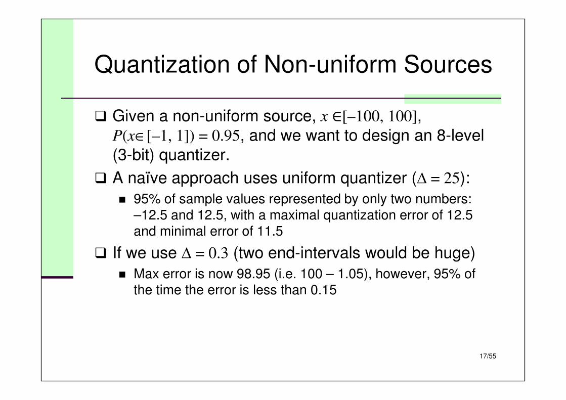
Quantization of Non-uniform Sources
� Given a non-uniform source, x ∈[–100, 100],
P(x∈[–1, 1]) = 0.95, and we want to design an 8-level
(3-bit) quantizer.
� A naïve approach uses uniform quantizer (∆ = 25):
� 95% of sample values represented by only two numbers:–12.5 and 12.5, with a maximal quantization error of 12.5 and minimal error of 11.5
� If we use ∆ = 0.3 (two end-intervals would be huge)
� Max error is now 98.95 (i.e. 100 – 1.05), however, 95% of the time the error is less than 0.15
18/55
Optimal ∆ that minimizes MSQE
� Given pdf fX(x) of the source, let’s design an M-level
mid-rise uniform quantizer that minimizes MSQE:
.)(2
12
)(2
122
12
2
1
1)1(
2
22
∫
∑∫
∞
∆
−
−
=
∆
∆−
∆
−−+
∆
−−=
M X
i
i
iXq
dxxfM
x
dxxfi
x
M
σ → Granular error
→ Overload error
x – Q(x)
Overload error
Granular error
19/55
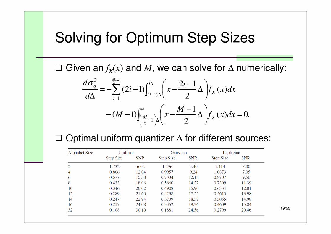
Solving for Optimum Step Sizes
� Given an fX(x) and M, we can solve for ∆ numerically:
� Optimal uniform quantizer ∆ for different sources:
.0)(2
1)1(
)(2
12)12(
12
1
1)1(
22
∫
∑ ∫∞
∆
−
−
=
∆
∆−
=
∆
−−−−
∆
−−−−=
∆
M X
i
i
iX
q
dxxfM
xM
dxxfi
xid
dM
σ
20/55
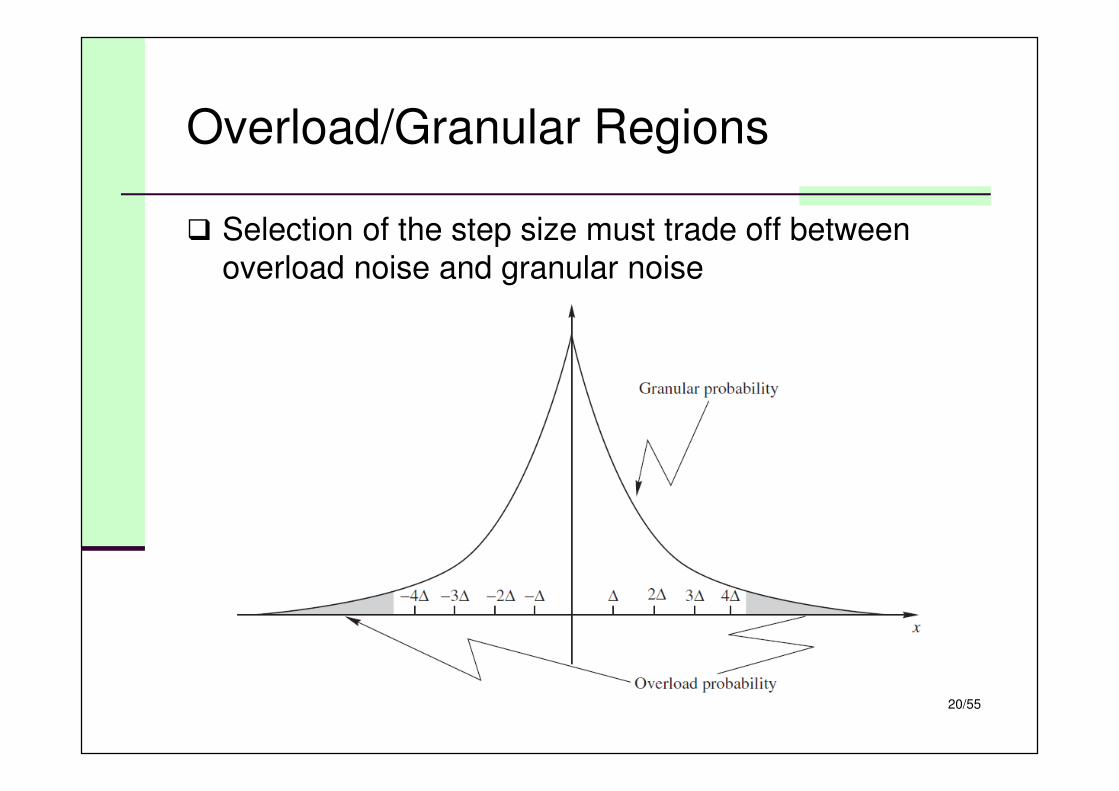
Overload/Granular Regions
� Selection of the step size must trade off between
overload noise and granular noise
21/55
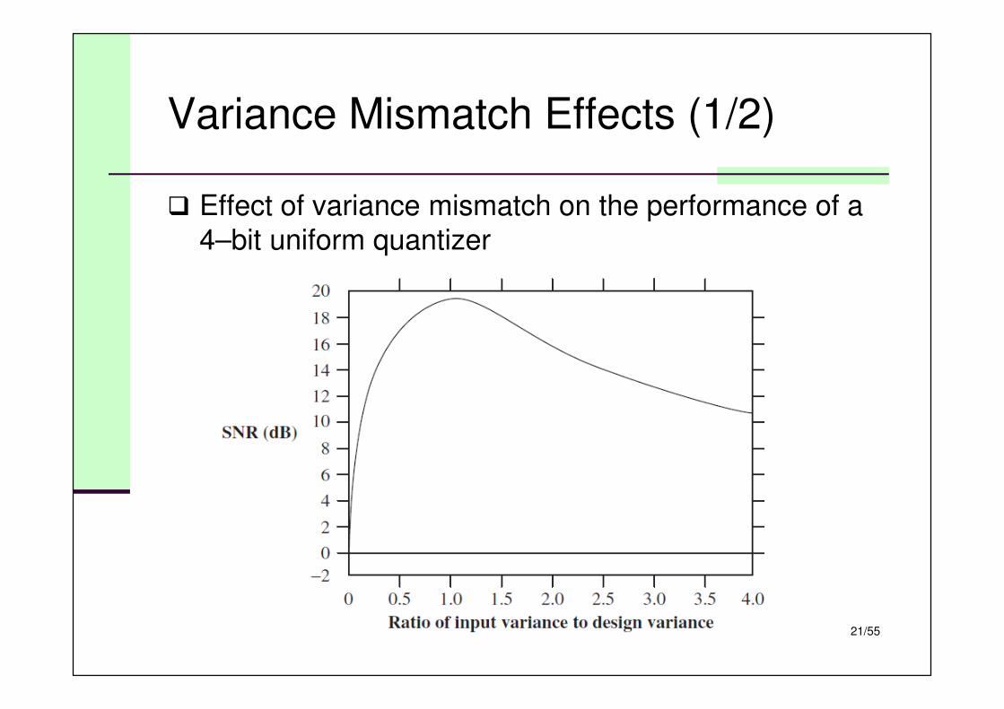
Variance Mismatch Effects (1/2)
� Effect of variance mismatch on the performance of a
4–bit uniform quantizer
22/55
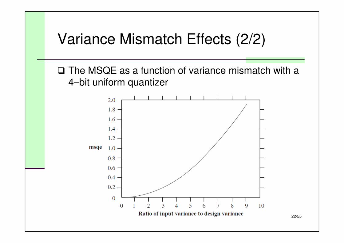
Variance Mismatch Effects (2/2)
� The MSQE as a function of variance mismatch with a
4–bit uniform quantizer
23/55
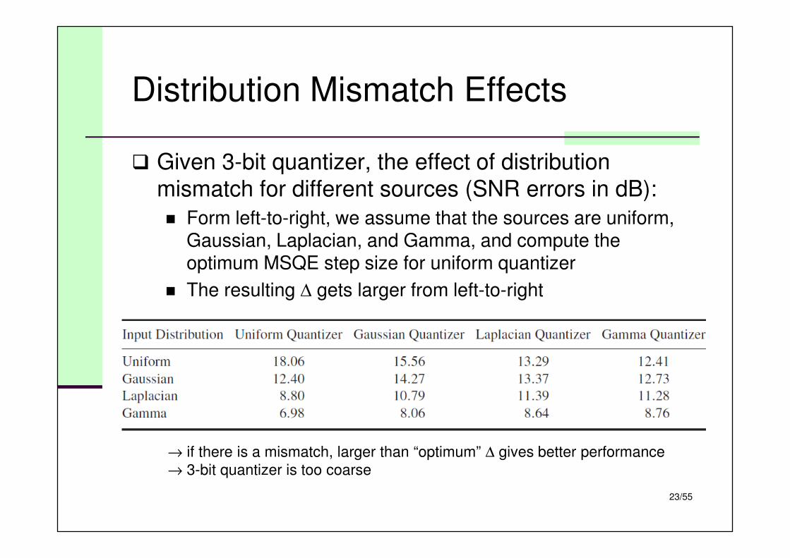
Distribution Mismatch Effects
� Given 3-bit quantizer, the effect of distribution
mismatch for different sources (SNR errors in dB):
� Form left-to-right, we assume that the sources are uniform, Gaussian, Laplacian, and Gamma, and compute the optimum MSQE step size for uniform quantizer
� The resulting ∆ gets larger from left-to-right
→ if there is a mismatch, larger than “optimum” ∆ gives better performance
→ 3-bit quantizer is too coarse
24/55
Adaptive Quantization
� We can adapt the quantizer to the statistics of the
input (mean, variance, pdf)
� Forward adaptive (encoder-side analysis)
� Divide input source in blocks
� Analyze block statistics
� Set quantization scheme
� Send the scheme to the decoder via side channel
� Backward adaptive (decoder-side analysis)
� Adaptation based on quantizer output only
� Adjust ∆ accordingly (encoder-decoder in sync)
� No side channel necessary
25/55
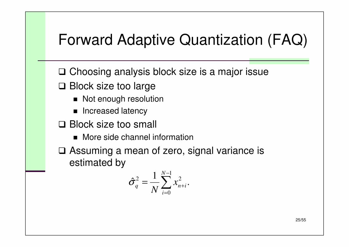
Forward Adaptive Quantization (FAQ)
� Choosing analysis block size is a major issue
� Block size too large
� Not enough resolution
� Increased latency
� Block size too small
� More side channel information
� Assuming a mean of zero, signal variance is
estimated by
.1
ˆ1
0
22 ∑−
=
+=N
i
inq xN
σ
26/55
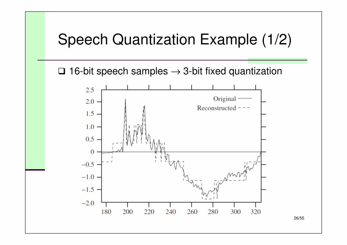
Speech Quantization Example (1/2)
� 16-bit speech samples → 3-bit fixed quantization
27/55
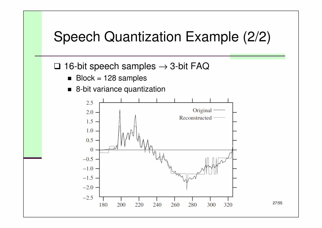
Speech Quantization Example (2/2)
� 16-bit speech samples → 3-bit FAQ
� Block = 128 samples
� 8-bit variance quantization
28/55
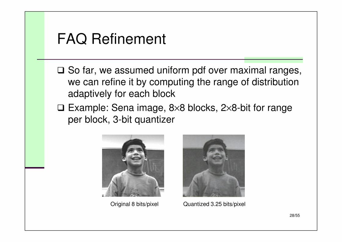
FAQ Refinement
� So far, we assumed uniform pdf over maximal ranges,
we can refine it by computing the range of distribution
adaptively for each block
� Example: Sena image, 8×8 blocks, 2×8-bit for range
per block, 3-bit quantizer
Original 8 bits/pixel Quantized 3.25 bits/pixel
29/55
Backward Adaptive Quantization (BAQ)
� Key idea: only encoder sees input source, if we do
not want to use side channel to tell the decoder how
to adapt the quantizer, we can only use quantized
output to adapt the quantizer
� Possible solution:
� Observe the number of output values that falls in outer levels and inner levels
� If they match the assumed pdf, ∆ is good
� If too many values fall in outer levels, ∆ should be enlarged, otherwise, ∆ should be reduced
� Issue: estimation of pdf requires large observations?
30/55
Jayant Quantizer
� N. S. Jayant showed in 1973 that ∆ adjustment based
on few observations still works fine:
� If current input falls in the outer levels, expand step size
� If current input falls in the inner levels, contract step size
� The total product of expansions and contraction should be 1
� Each decision interval k has a multiplier Mk
� If input sn–1 falls in the kth interval, step size is multiplied by Mk
� Inner-level Mk < 1, outer-level Mk > 1
� Step size adaptation rule:
where l(n–1) is the quantization interval at time n–1.
,1)1( −− ∆=∆ nnln M
31/55
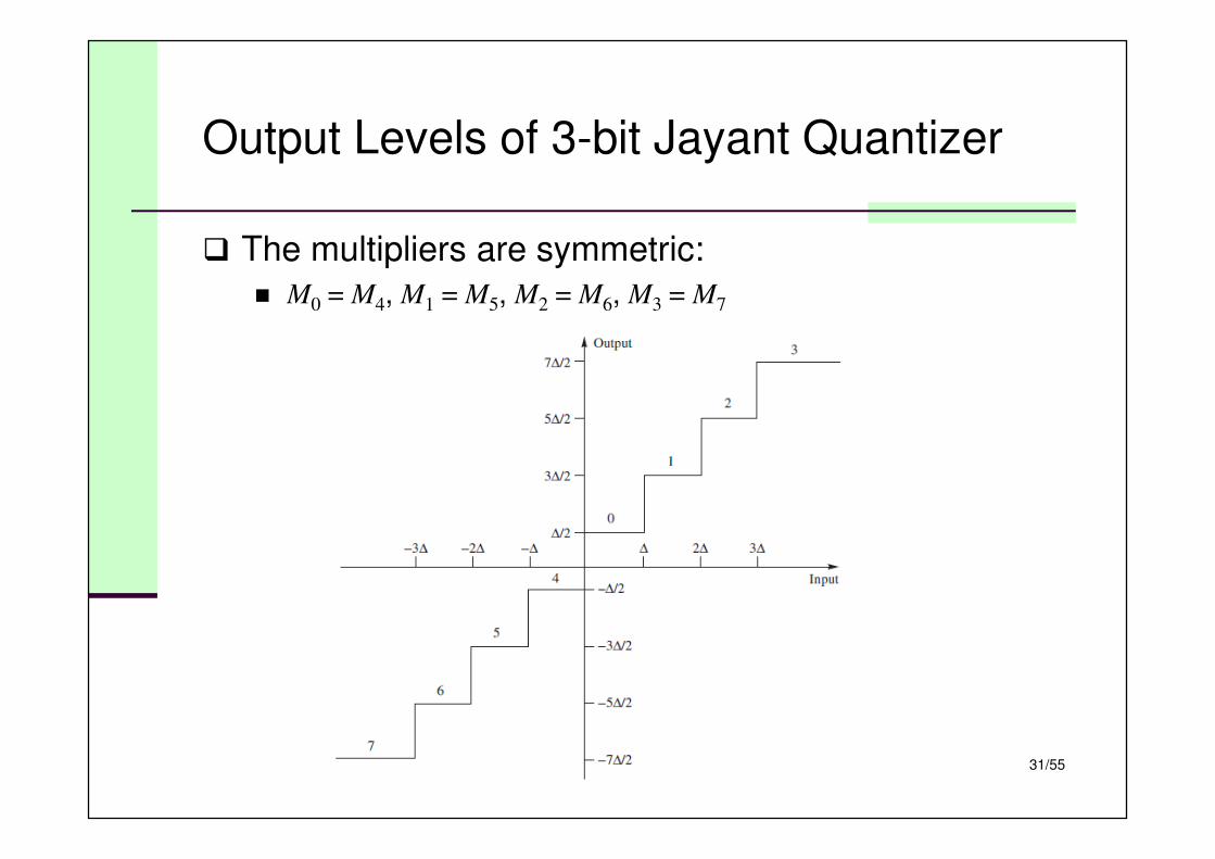
Output Levels of 3-bit Jayant Quantizer
� The multipliers are symmetric:
� M0 = M4, M1 = M5, M2 = M6, M3 = M7
32/55
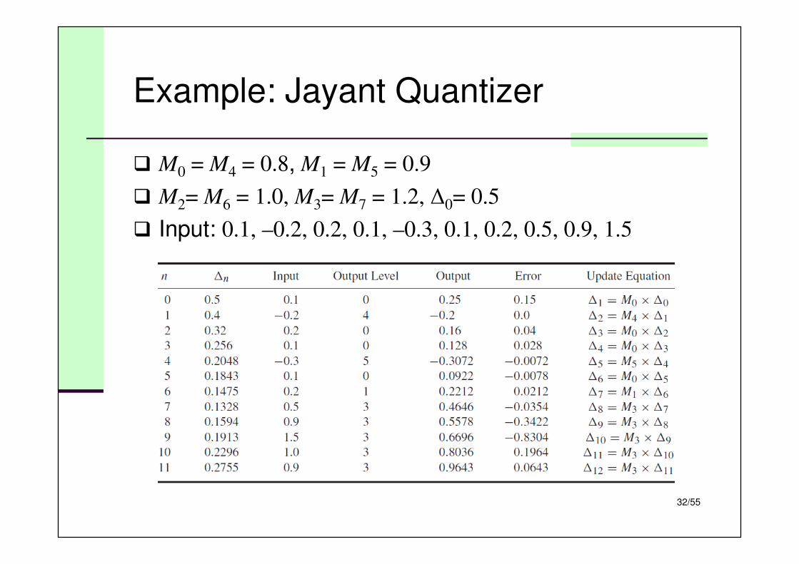
Example: Jayant Quantizer
� M0 = M4 = 0.8, M1 = M5 = 0.9
� M2= M6 = 1.0, M3= M7 = 1.2, ∆0= 0.5
� Input: 0.1, –0.2, 0.2, 0.1, –0.3, 0.1, 0.2, 0.5, 0.9, 1.5
33/55
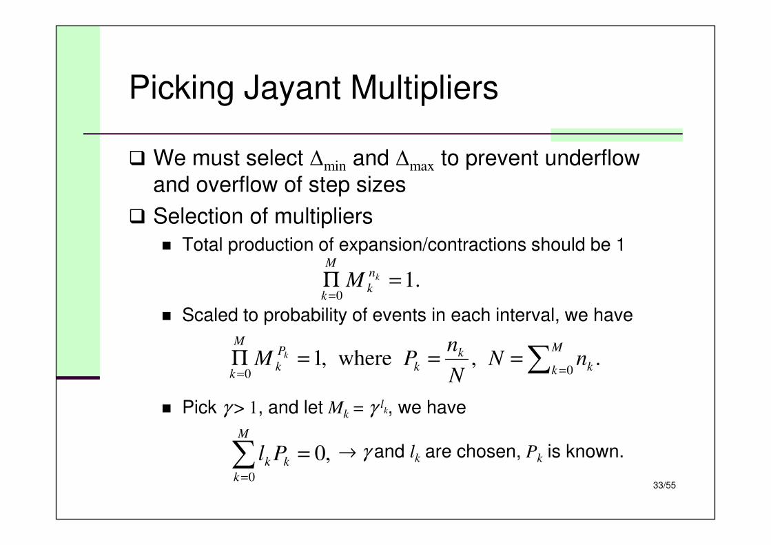
Picking Jayant Multipliers
� We must select ∆min and ∆max to prevent underflow
and overflow of step sizes
� Selection of multipliers
� Total production of expansion/contractions should be 1
� Scaled to probability of events in each interval, we have
� Pick γ > 1, and let Mk = γ lk, we have
→ γ and lk are chosen, Pk is known.
.10
=Π=
kn
k
M
kM
.,where,100
∑ =====Π
M
k kk
k
P
k
M
knN
N
nPM k
,00
=∑=
M
k
kk Pl
34/55
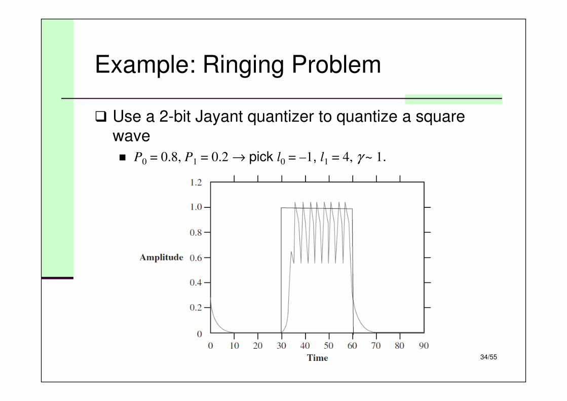
Example: Ringing Problem
� Use a 2-bit Jayant quantizer to quantize a square
wave
� P0 = 0.8, P1 = 0.2 → pick l0 = –1, l1 = 4, γ ~ 1.
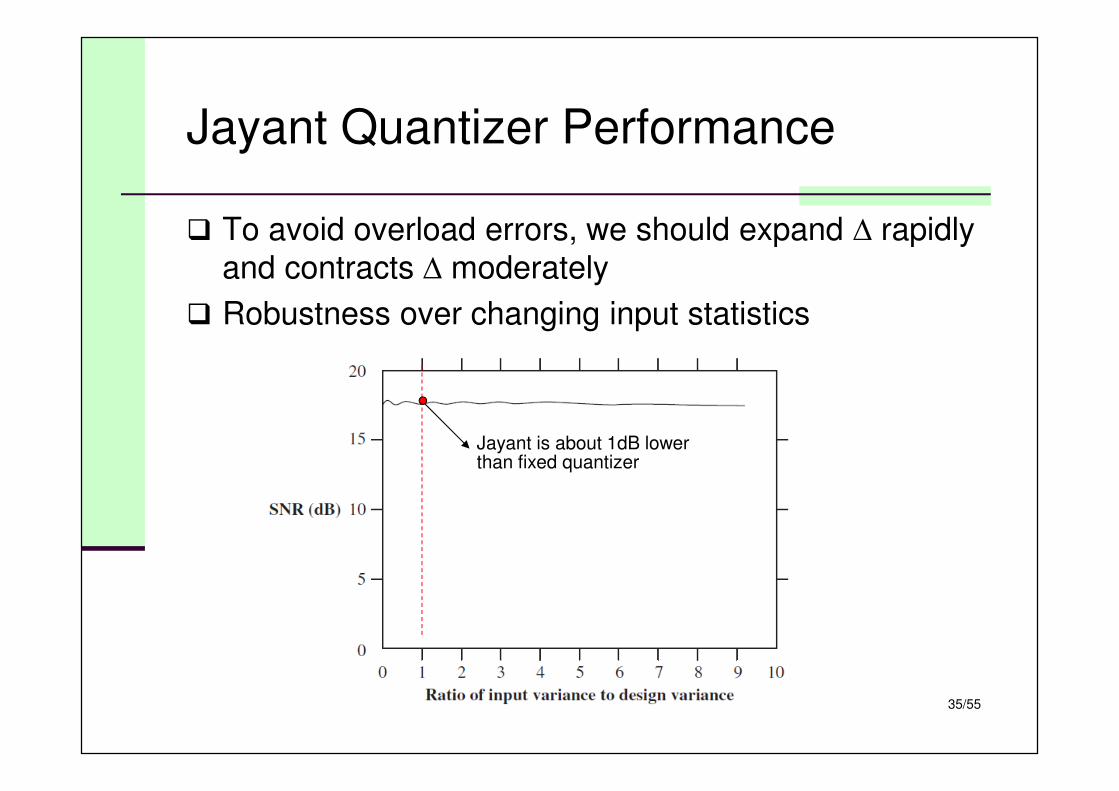
� To avoid overload errors, we should expand ∆ rapidly
and contracts ∆ moderately
� Robustness over changing input statistics
35/55
Jayant Quantizer Performance
Jayant is about 1dB lowerthan fixed quantizer
36/55
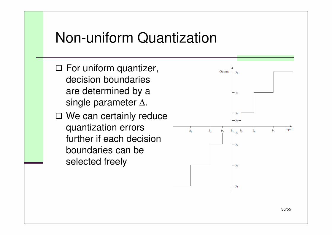
Non-uniform Quantization
� For uniform quantizer,
decision boundaries
are determined by a
single parameter ∆.
� We can certainly reduce
quantization errors
further if each decision
boundaries can be
selected freely
37/55
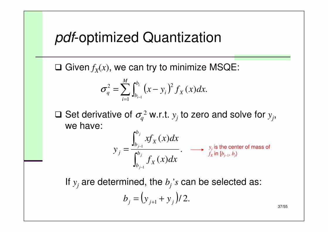
pdf-optimized Quantization
� Given fX(x), we can try to minimize MSQE:
� Set derivative of σq2 w.r.t. yj to zero and solve for yj,
we have:
If yj are determined, the bj’s can be selected as:
( ) .)(1
22
1∑∫
= −
−=M
i
b
bXiq
i
i
dxxfyxσ
.)(
)(
1
1
∫
∫
−
−=j
j
j
j
b
bX
b
bX
j
dxxf
dxxxf
y
( ) .2/1 jjj yyb += +
yj is the center of mass offX in [bj–1, bj)
38/55
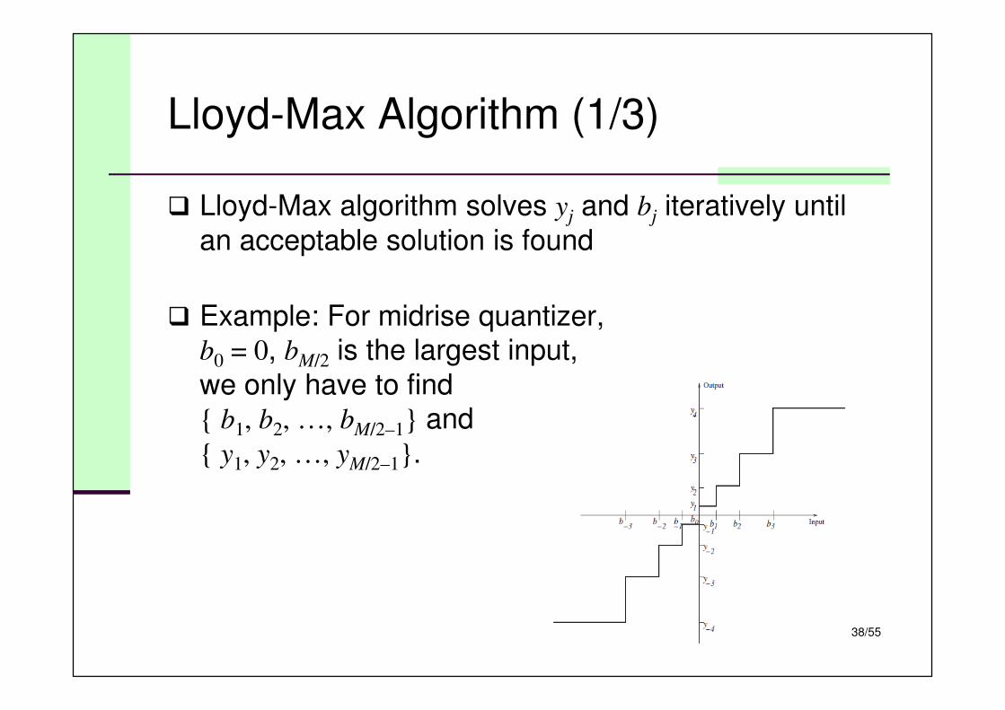
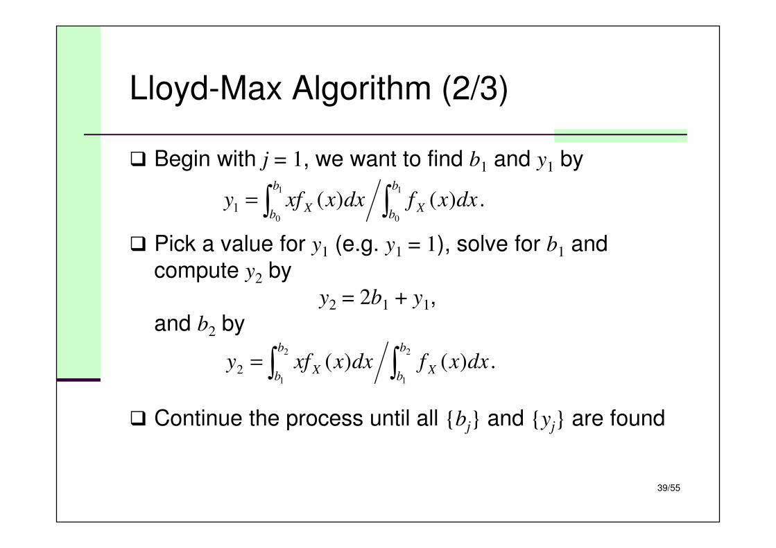
Lloyd-Max Algorithm (1/3)
� Lloyd-Max algorithm solves yj and bj iteratively until
an acceptable solution is found
� Example: For midrise quantizer,b0 = 0, bM/2 is the largest input,
we only have to find{ b1, b2, …, bM/2–1} and
{ y1, y2, …, yM/2–1}.
39/55
Lloyd-Max Algorithm (2/3)
� Begin with j = 1, we want to find b1 and y1 by
� Pick a value for y1 (e.g. y1 = 1), solve for b1 and
compute y2 by
y2 = 2b1 + y1,
and b2 by
� Continue the process until all {bj} and {yj} are found
.)()(1
0
1
01 ∫∫=
b
bX
b
bX dxxfdxxxfy
.)()(2
1
2
12 ∫∫=
b
bX
b
bX dxxfdxxxfy
40/55
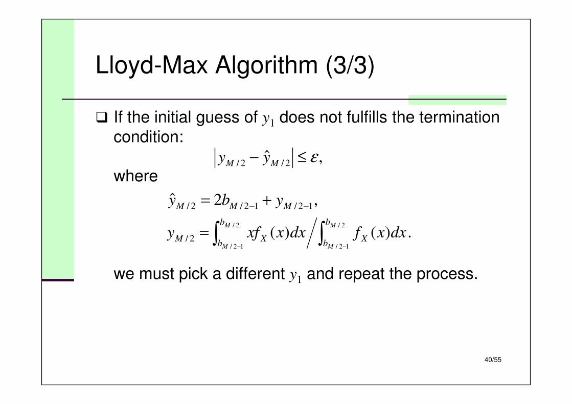
Lloyd-Max Algorithm (3/3)
� If the initial guess of y1 does not fulfills the termination
condition:
where
we must pick a different y1 and repeat the process.
,ˆ2/2/ ε≤− MM yy
,2ˆ12/12/2/ −− += MMM yby
.)()(2/
12/
2/
12/2/ ∫∫
−−
=M
M
M
M
b
bX
b
bXM dxxfdxxxfy
41/55
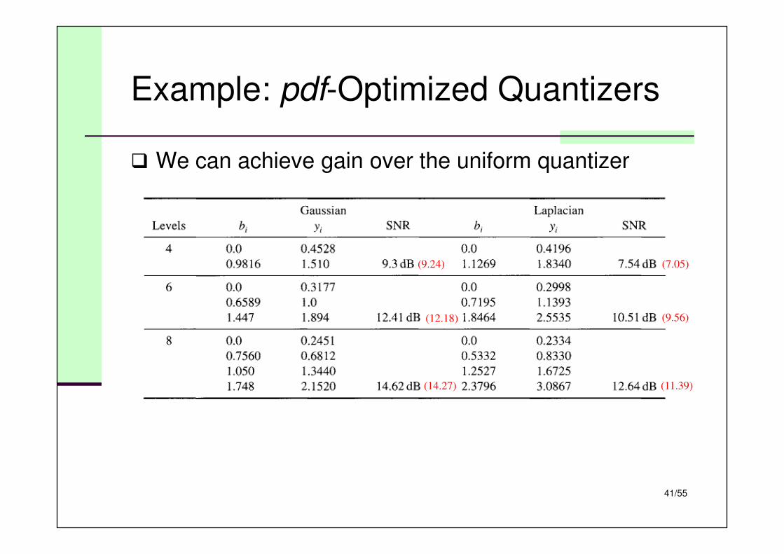
Example: pdf-Optimized Quantizers
� We can achieve gain over the uniform quantizer
(9.24) (7.05)
(12.18) (9.56)
(14.27) (11.39)
42/55
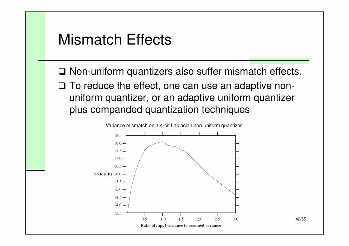
Mismatch Effects
� Non-uniform quantizers also suffer mismatch effects.
� To reduce the effect, one can use an adaptive non-
uniform quantizer, or an adaptive uniform quantizer
plus companded quantization techniques
Variance mismatch on a 4-bit Laplacian non-uniform quantizer.
43/55
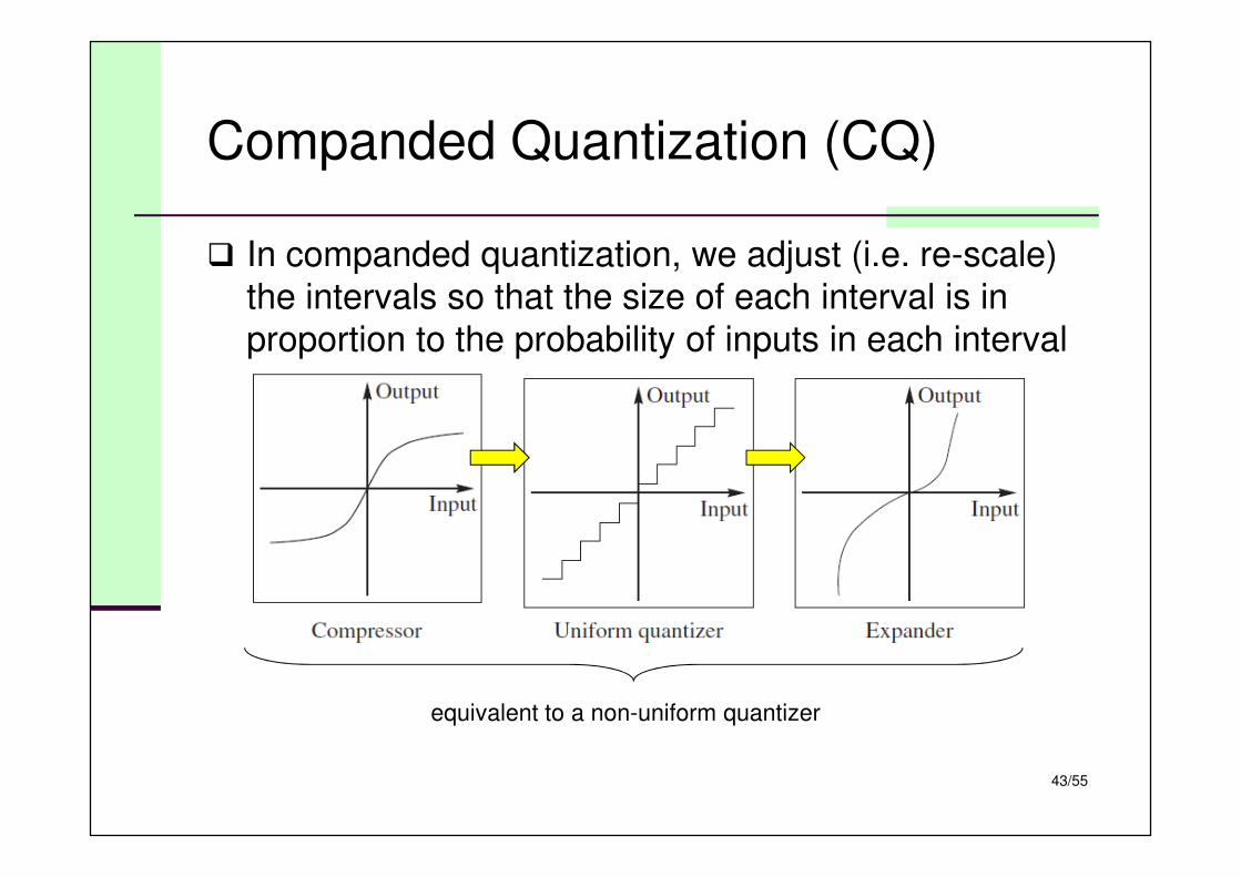
Companded Quantization (CQ)
� In companded quantization, we adjust (i.e. re-scale)
the intervals so that the size of each interval is in
proportion to the probability of inputs in each interval
equivalent to a non-uniform quantizer
44/55
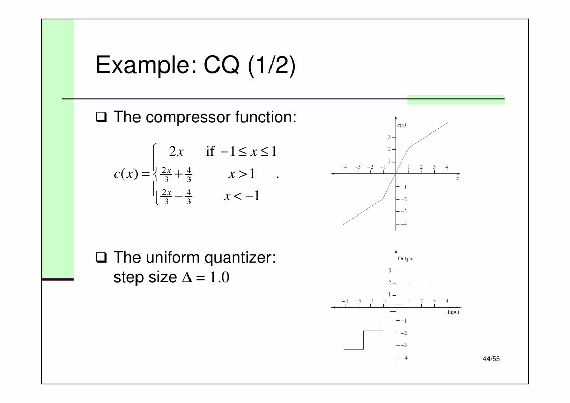
Example: CQ (1/2)
� The compressor function:
� The uniform quantizer:step size ∆ = 1.0
.
1
1
11if2
)(
34
32
34
32
−<−
>+
≤≤−
=
x
x
xx
xc
x
x
45/55
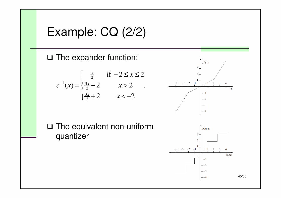
Example: CQ (2/2)
� The expander function:
� The equivalent non-uniform
quantizer
.
22
22
22if
)(
23
23
2
1
−<+
>−
≤≤−
=−
x
x
x
xc
x
x
x
46/55
Remarks on CQ
� If the level of quantizer is large and the input is bounded by xmax, it is possible to choose a c(x) such
that the SNR of CQ is independent to the input pdf:
SNR = 10 log10(3M2) – 20log10 α,
where c′(x) = xmax / (α |x|) and a is a constant.
� Two popular CQ for telephones: µ-law and A-law
� µ-law compressor
� A-law compressor
).sgn()1ln(
)1ln()( max
max xxxcx
x
µ
µ
+
+=
.1),sgn(
0),sgn()(
max
max
max
1ln1
ln1
max
1ln1
≤≤⋅
≤≤=
+
+
+
x
x
AA
Ax
x
A
xA
xx
xxc
x
xA
47/55
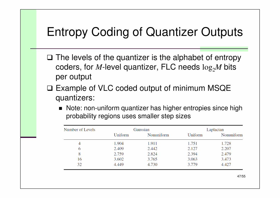
Entropy Coding of Quantizer Outputs
� The levels of the quantizer is the alphabet of entropy coders, for M-level quantizer, FLC needs log2M bits
per output
� Example of VLC coded output of minimum MSQE
quantizers:
� Note: non-uniform quantizer has higher entropies since high probability regions uses smaller step sizes
48/55
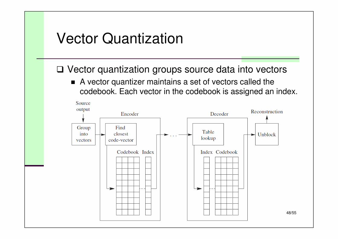
Vector Quantization
� Vector quantization groups source data into vectors
� A vector quantizer maintains a set of vectors called the codebook. Each vector in the codebook is assigned an index.
49/55
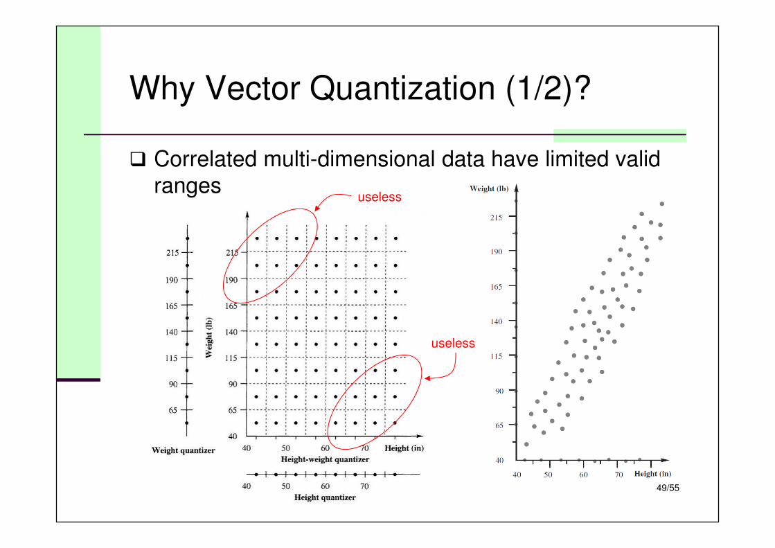
Why Vector Quantization (1/2)?
� Correlated multi-dimensional data have limited valid
rangesuseless
useless
50/55
Why Vector Quantization (2/2)?
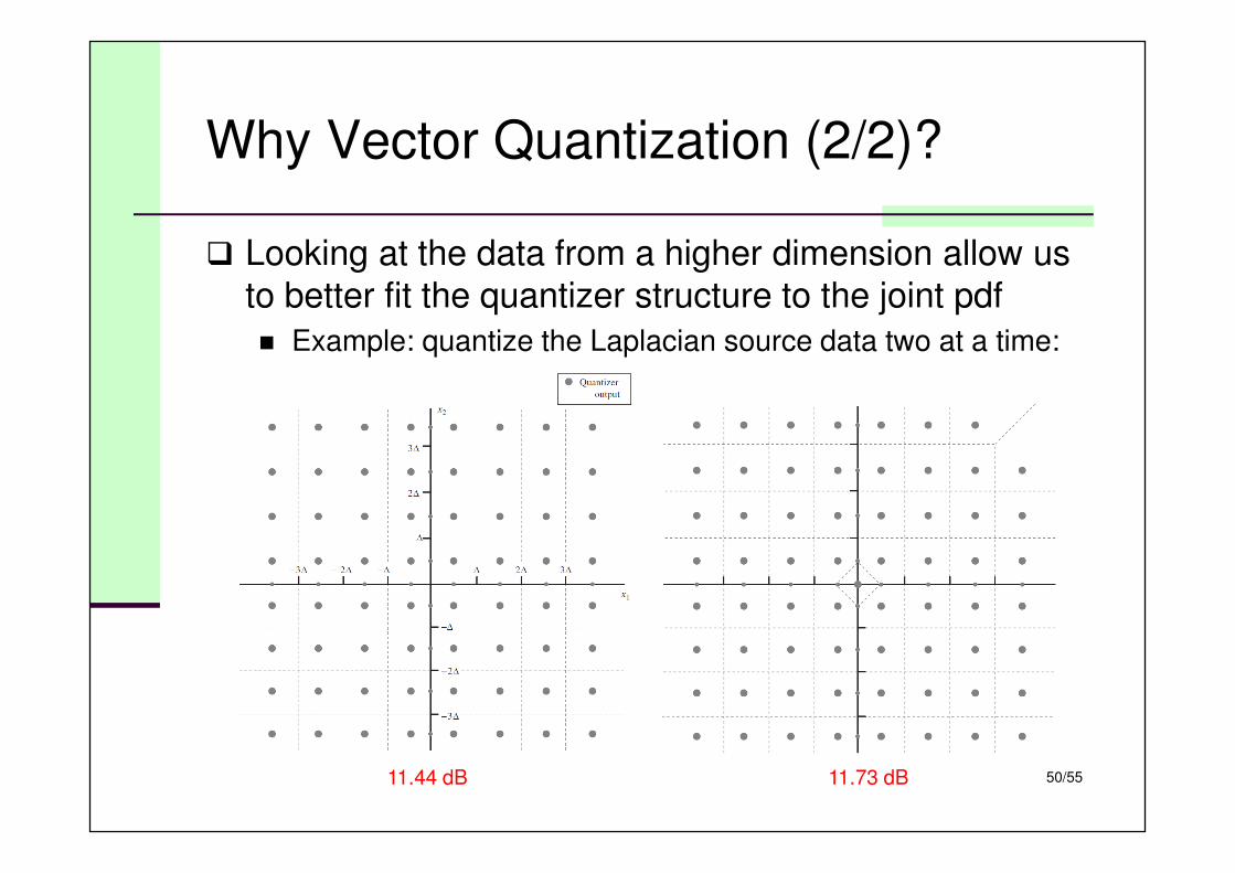
� Looking at the data from a higher dimension allow us
to better fit the quantizer structure to the joint pdf
� Example: quantize the Laplacian source data two at a time:
11.44 dB 11.73 dB
51/55
Vector Quantization Rule
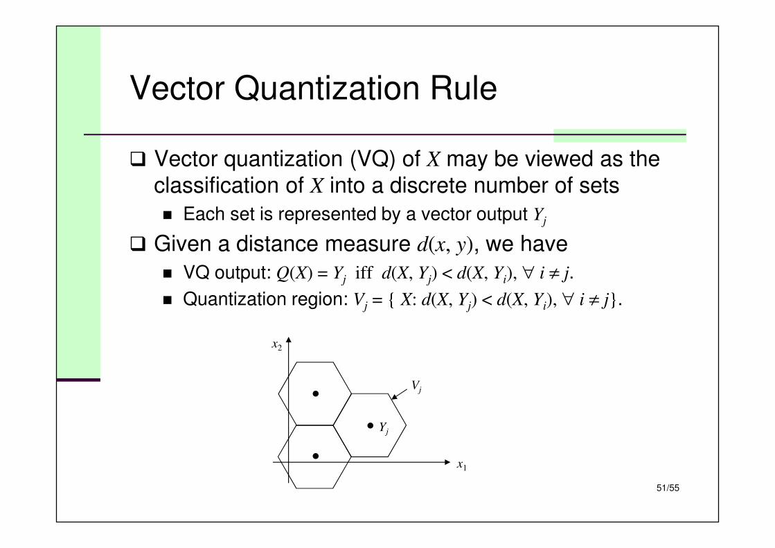
� Vector quantization (VQ) of X may be viewed as the
classification of X into a discrete number of sets
� Each set is represented by a vector output Yj
� Given a distance measure d(x, y), we have
� VQ output: Q(X) = Yj iff d(X, Yj) < d(X, Yi), ∀ i ≠ j.
� Quantization region: Vj = { X: d(X, Yj) < d(X, Yi), ∀ i ≠ j}.
Vj
Yj
x1
x2
52/55
Codebook Design
� The set of quantizer output points in VQ is called the codebookof the quantizer, and the process of placing these output points is often referred to as the codebook design
� The k-means algorithm† is often used to classify the outputs
� Given a large set of output vectors from the source, known as the training set, and an initial set of k representative patterns
� Assign each element of the training set to the closest
representative pattern
� After an element is assigned, the representative pattern is updated
by computing the centroid of the training set vectors assigned to it
� When the assignment process is complete, we will have k groups of
vectors clustered around each of the output points
† The idea is the same as the scalar quantization problem in Stuart P. Lloyd, “Least Squares Quantization in PCM,” IEEE
Trans. on Information Theory, Vol. 28, No. 2, March 1982.
53/55
The Linde-Buzo-Gray Algorithm
1. Start with an initial set of reconstruction values {Yi
(0)}i=1..M and a set of training vectors {Xn}n=1..N.
Set k = 0, D(0) = 0. Select threshold ε.
2. The quantization regions {Vi(k)}i=1..M are given by
Vj(k) = {Xn: d(Xn, Yi) < d(Xn, Yj), ∀ j ≠ i}, i = 1, 2, …, M.
3. Compute the average distortion D(k) between the
training vectors and the representative value
4. If (D(k) – D(k–1))/D(k) < ε, stop; otherwise, continue
5. Let k = k + 1. Update {Yi(k)}i=1..M with the average
value of each quantization region Vi(k–1). Go to step 2.
54/55
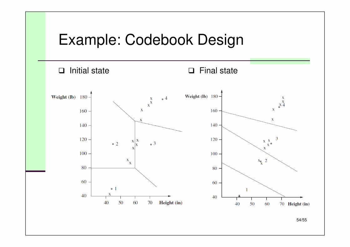
Example: Codebook Design
� Initial state � Final state
55/55
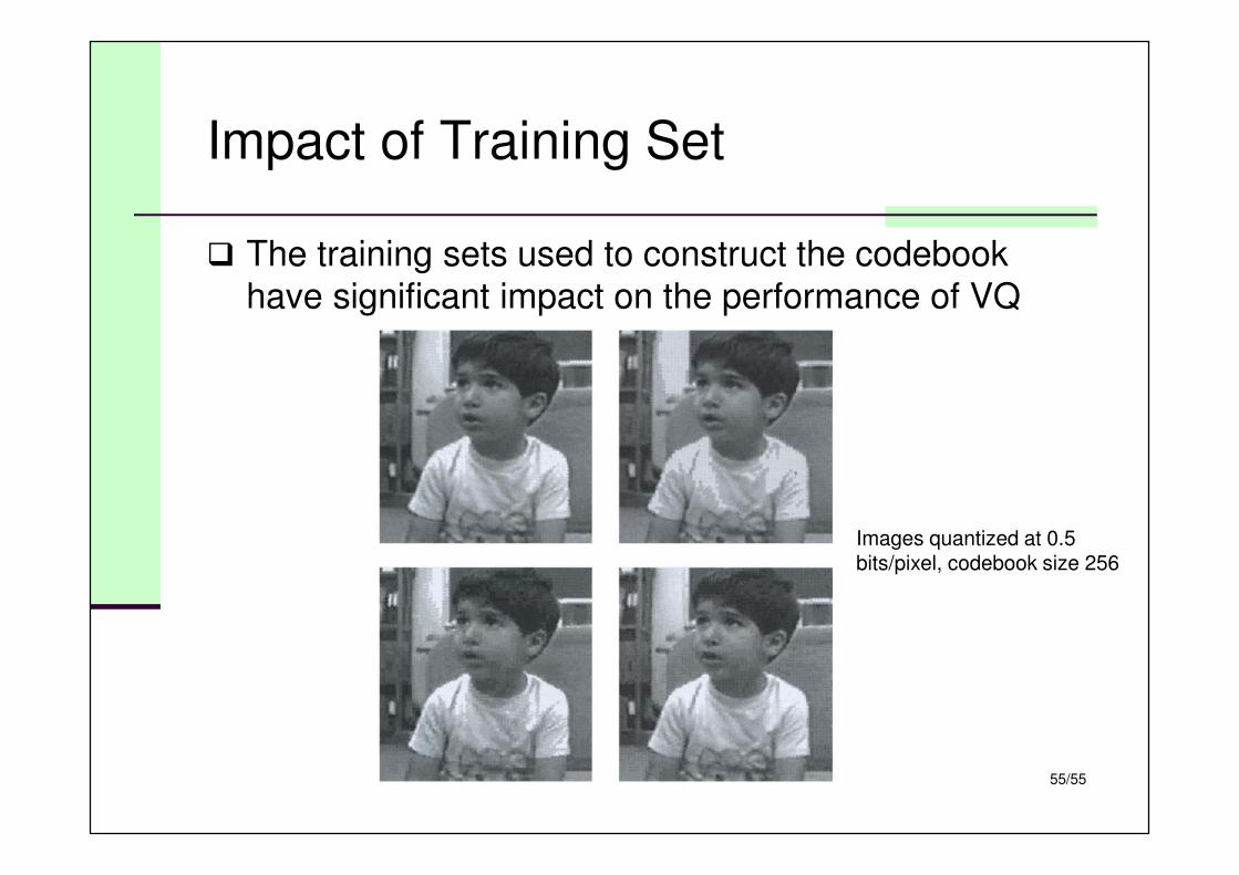
Impact of Training Set
� The training sets used to construct the codebook
have significant impact on the performance of VQ
Images quantized at 0.5 bits/pixel, codebook size 256

![· Senaraikan dan beri contoh dua kategori dalam kuantitifizik. [4 marks] [4 markah] Define scalar quantity and vector quantity with TWO (2) examples each. Terangkan kuantiti skalar](https://img.pdfslide.tips/doc/110x75/5e2a93abb7ff770801364c45/senaraikan-dan-beri-contoh-dua-kategori-dalam-kuantitifizik-4-marks-4-markah.jpg)