Signal Processing & Fourier Analysis

James P. LeBlanc

Prof. of Signal Processing

Lulea University of Technology

1

Short Course Outline

• Day 1⋄ Introduction & History⋄ Mathematical Preparation/Context⋄ Fourier Series⋄ Lunch Break⋄ Lab work I

• Day 2⋄ L2 Theory⋄ Fourier Transform⋄ Discrete Fourier⋄ Points in Space (a digression)⋄ Applications⋄ Lunch Break⋄ Lab work II

2

Introduction & History

3

Course Material

Course material will be drawn from

• “Fourier Analysis and Its Applications” by Anders Vretbland, Springer.

• Some personal notes and perspectives

4

Fourier?

What do you think of when you hear the term “Fourier” ??

5

Fourier, the person

• Jean Baptiste Joseph Fourier 1768-1830

• French mathematician and physicist

• discovered “greenhouse effect”

• studied heat transfer

• “Theorie Analytique de la Chaleur” (1822)

• known for Fourier Series, Fourier Transform

6

Some Notation

• LaPlace Operator = ∇2 = ∂2

∂x2 + ∂2

∂y2 + ∂2

∂z2

• partial with respect to time ut = ∂u∂t

• second partial uxy = ∂2u∂x∂y

• denote 3-d space as Ω = [x y z]

7

Well-posed Problems

A problem is said to be “well-posed” when all three conditions are met:

• there exists a solution to the problem

• there existsonly onesolution

• the solution isstable(small changes in equation parameters produce

small changes in solution)

8

Some Important Historical Physical Equations

• The Wave Equation

• The Heat Equation

• The LaPlace Equation

• The Poisson Equation

We’ll look at the first two more closely.

9

The Wave Equation

u =∂2u∂x2 +

∂2u∂y2 +

∂2u∂z2 =

1c2

∂2u∂t2 (x, t) ∈ Ω×T

• u(t,x) is the displacement at timet point x

• c is a constant depending on properties of material

• describes vibrations in a homogeneous medium

• reversible process

On a string, we can write:

∂2u∂x2 =

1c2

∂2u∂t2

10

One Dimensional Wave Equation

c2 ∂2u∂x2 =

∂2u∂t2

• Consider a sol’n in open half planet > 0

• introduce new coordinatesξ = x−ct, andη = x+ct

• ∂2u∂x2 =

∂2u∂ξ2 +2

∂2u∂ξ∂η

+∂2u∂η2

• ∂2u∂t2 = c2

(∂2u∂ξ2 −2

∂2u∂ξ∂η

+∂2u∂η2

)

11

One Dimensional Wave Equation (cont.)

• Inserting these into equation yields:

c2 4∂2u

∂ξ∂η= 0 ⇔ ∂

∂ξ

(∂u∂η

)

= 0

• We see∂u∂η

is only a function ofη, say∂u∂η

= h(η)

• Let φ be antiderivative ofh, then another integration yieldsu = φ(η)+ψ(n), whereφ is a new arbitrary function.

• returning to original variables(x, t) we have found thatu(x, t) = φ(x−ct)+ψ(x+ct)

• φ andψ are more or less arbitrary functions of one variable.

• Note motion “to the left” and “to the right”

12

The Heat Equation / The Diffusion Equation

u =∂2u∂x2 +

∂2u∂y2 +

∂2u∂z2 =

1a2

∂u∂t

(x, t) ∈ Ω×T

• u(t,x) is the temperature at timet at pointx

• describes the heat flow per unit time

• a is a constant depending on properties of material

• irreversible process

13

Fourier’s Method (Theorie Analytique de la Chaleur-1822)

• Attempt to solve Heat Equation∂2u∂x2 =

∂u∂t

• assume rod of lengthπ

• keep each end at temperature zero u(0, t) = u(π, t) = 0

• assume an initial temperature distribution within rod isf (x) = u(x,0)

x=0 x=π

Initial Conditions

f(x)=u(x,0)

u(0,t)=0 u( ,t)=0πBoundary Conditions

14

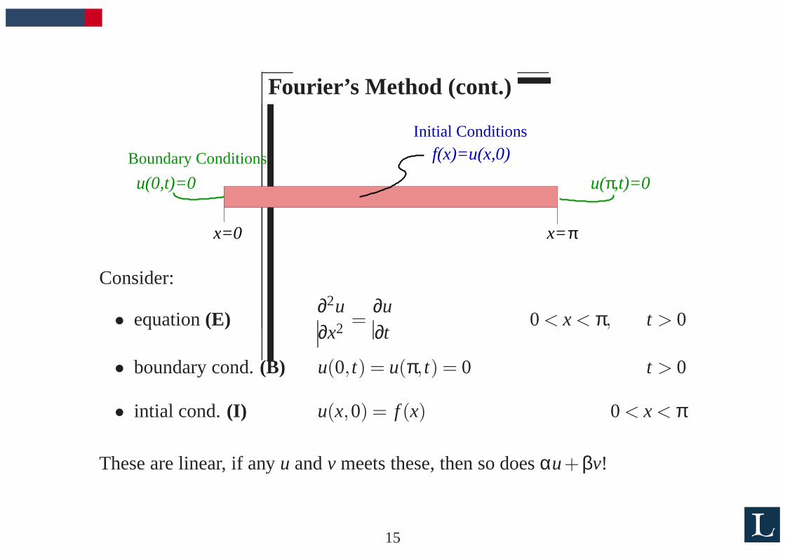
Fourier’s Method (cont.)

x=0 x=π

Initial Conditions

f(x)=u(x,0)

u(0,t)=0 u( ,t)=0πBoundary Conditions

Consider:

• equation(E)∂2u∂x2 =

∂u∂t

0 < x < π, t > 0

• boundary cond.(B) u(0, t) = u(π, t) = 0 t > 0

• intial cond.(I) u(x,0) = f (x) 0 < x < π

These are linear, if anyu andv meets these, then so doesαu+βv!

15

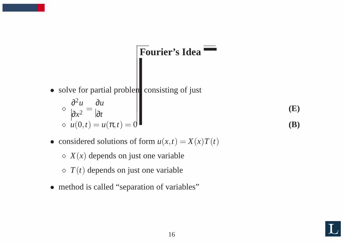
Fourier’s Idea

• solve for partial problem consisting of just

⋄ ∂2u∂x2 =

∂u∂t

(E)

⋄ u(0, t) = u(π, t) = 0 (B)

• considered solutions of formu(x, t) = X(x)T(t)

⋄ X(x) depends on just one variable

⋄ T(t) depends on just one variable

• method is called “separation of variables”

16

Fourier’s Idea (cont.)

• when considering solutions of formu(x, t) = X(x)T(t) then(E),

∂2u∂x2 =

∂u∂t

becomes X′′(x)T(t) = X(x)T ′(t) 0 < x < π, t > 0

• rearrange as

X′′(x)X(x)

=T ′(t)T(t)

0 < x < π, t > 0

• has peculiar property that if we changet → LHS is uneffected→ RHS

is also uneffected. So this must be aconstant(call this−λ)

• Similarly for changes ofx

17

Fourier’s Idea (cont.)

• So, we have now −λ =X′′(x)X(x)

=T ′(t)T(t)

• or,

X′′(x)+λX(x) = 0 0< x < π

T ′(t)+λT(t) = 0 t > 0

• including(B) by u(x, t) = X(x)T(t) yields:

⋄ X(0)T(t) = X(π)T(t) = 0 t > 0

⋄ if X(0) 6= 0 → T(t) = 0 for t > 0 ⇒ u(x, t) = 0 (trivial sol’n)

⋄ to get interesting sol’n, we must demandX(0) = X(π) = 0

18

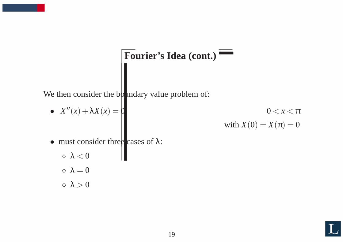
Fourier’s Idea (cont.)

We then consider the boundary value problem of:

• X′′(x)+λX(x) = 0 0 < x < π

with X(0) = X(π) = 0

• must consider three cases ofλ:

⋄ λ < 0

⋄ λ = 0

⋄ λ > 0

19

Caseλ < 0

X′′(x)+λX(x) = 0, X(0) = X(π) = 0,

• can writeλ = −α2, and assumeα > 0, yielding X′′(x)−α2X(x) = 0

• general sol’n is X(x) = Aeαx +Be−αx

• (B) becomes 0 = X(0) = A+B

0 = X(π) = Aeαπ +Be−απ

• homogenous linear system of equations, two equations, two unknowns

• this hasuninteresting, unique sol’n A = B = 0

• thenX(x) is trivial (and uninteresting)

20

Caseλ = 0

X′′(x)+λX(x) = 0, X(0) = X(π) = 0,

• differential equation reduces to X′′(x) = 0

• this has solution X(x) = Ax+B

• again(B), X(0) = X(π) = 0 ⇒ A = B = 0

• X(x) is again trivial (and uninteresting)

21

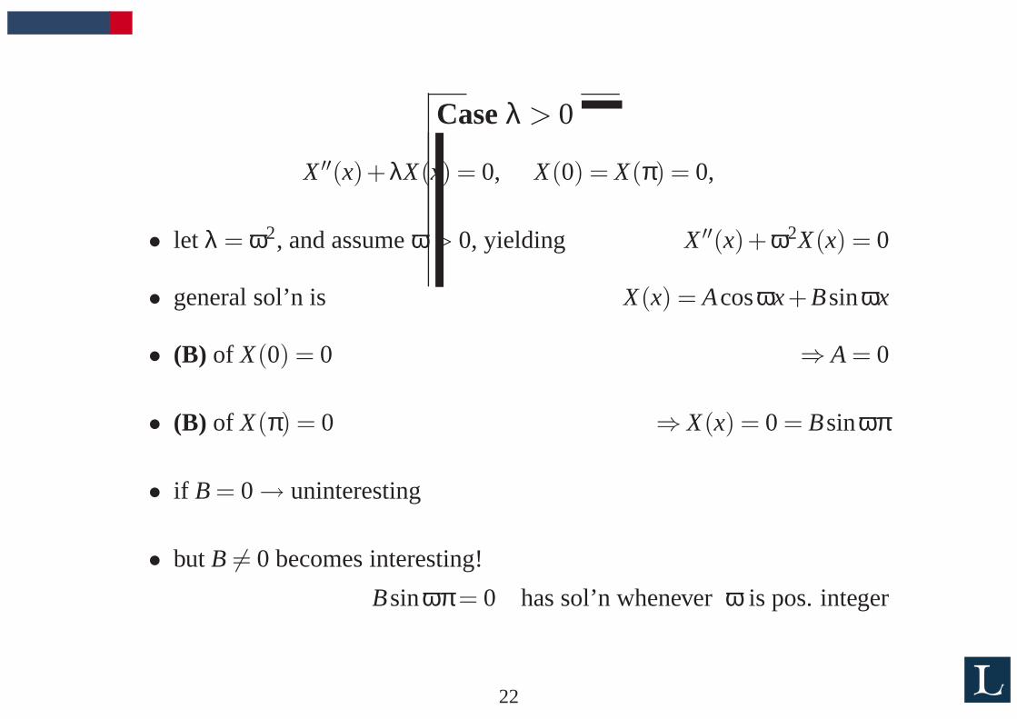
Caseλ > 0

X′′(x)+λX(x) = 0, X(0) = X(π) = 0,

• let λ = ω2, and assumeω > 0, yielding X′′(x)+ω2X(x) = 0

• general sol’n is X(x) = Acosωx+Bsinωx

• (B) of X(0) = 0 ⇒ A = 0

• (B) of X(π) = 0 ⇒ X(x) = 0 = Bsinωπ

• if B = 0→ uninteresting

• butB 6= 0 becomes interesting!

Bsinωπ = 0 has sol’n wheneverω is pos. integer

22

Almost!

• the problem X′′(x)+λX(x) = 0, 0< x < π, X(0) = X(π) = 0

• has non-trivial sol’n exactly for λ = n2 wheren is pos. integer

• this sol’n has form of X(x) = Xn(x) = Bn sinnx

whereBn is a constant

• For these values ofλ, let’s also solve T ′(t)+λT(t) = 0

T ′(t) = −n2T(t)

• This has general sol’n T(t) = Tn(t) = Cne−n2t

23

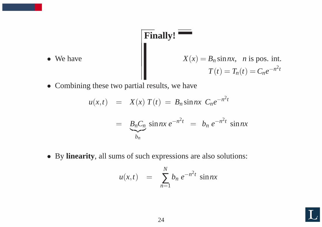
Finally!

• We have X(x) = Bn sinnx, n is pos. int.

T(t) = Tn(t) = Cne−n2t

• Combining these two partial results, we have

u(x, t) = X(x) T(t) = Bnsinnx Cne−n2t

= BnCn︸︷︷︸

bn

sinnx e−n2t = bn e−n2t sinnx

• By linearity , all sums of such expressions are also solutions:

u(x, t) =N

∑n=1

bn e−n2t sinnx

24

Summary of Fourier’s Result

• for (I) , initial conditions, of form

f (x) = u(x,0) =N

∑n=1

bn sinnx 0 < x < π

• for (B), boundary conditions u(0, t) = u(0,π) = 0

• one dimensional heat equation c2 ∂2u∂x2 =

∂2u∂t2

• has solutions of the form:

u(x, t) =N

∑n=1

bn e−n2t sinnx 0 < x < π, t > 0

25

Numerical Experiment of Fourier’s Result

• We use MATLAB with Fourier’s equation of solution to visualize twocases:

⋄ temperature in a bar with u(x,0) = f (x) = 12 sinx+ 1

2 sin3x

−1

−0.5

0

0.5

1 0.5*sin(x) + 0.5*sin(3x)

⋄ temperature in a bar with u(x,0) = f (x) with many terms

0 0.5 1 1.5 2 2.5 30

0.2

0.4

0.6

0.8

1

1.2 t = 0

26

Questions on Fourier’s Result

• Can we permitN → ∞ ?

• Is it possible to approximate anarbitrary function f (x) using sums of

sinusoids?

27

Remarks

• Initially, usefulness of Fourier’s results were met with some scepticism

• The extension off (x) to arbitrary functions was considered

controversial

• Ideas on convergence of function needed to be more fully developed to

assess situation

• The answer to these (and other questions) were a long time coming

(ending in 1960’s (?))

28

Some Mathematical & Notational Preparation

29

Euler’s Formula

• Euler’s Formula eiy = cosy+ i siny

eiy

Imagz

Realz

y

ycos

sin

C

30

Positive summation kernels (or distributions)

• let I = (−a,a) be an interval (finite or infinite)

• supposeKn(s)∞n=1 has properties

(1) Kn(s) ≥ 0, ∀s∈ I

(2)Z a

−aKn(s)ds= 1

(3) if δ > 0 , then limn→∞

Z

δ<|s|<aKn(s)ds= 0

• If f : I →C is integrable and bounded onI and continuous fors= 0,

we then have limn→∞

Z a

−aKn(s) f (s)ds= f (0)

31

Generalization of a Function

• Dirac Distribution (or “Delta Function”):

(1) δ(t) ≥ 0, −∞ < t < ∞

(2) δ(t) = 0, t 6= 0

(3)Z ∞

−∞δ(t)dt = 1

• Properties of Dirac Distribution:

⋄Z ∞

−∞δ(t)φ(t)dt = φ(0)

⋄Z ∞

−∞δ(t − τ)φ(t)dt = φ(τ)

32

Review of Some Linear System Theory

33

Laplace Transform

• Pierre Simon de Laplace,Theorie analytique des probabilites (1812)

• His methods “baffled his contemporaries”.

• Defined as:

f (s) =Z ∞

0f (t)e−stdt = L [ f (t)]

• Useful tool for solving linear differential equations withinitial value

conditions

• It is linearity L [α f (t)+βg(t)] = αL [ f (t)]+βL [g(t)]

34

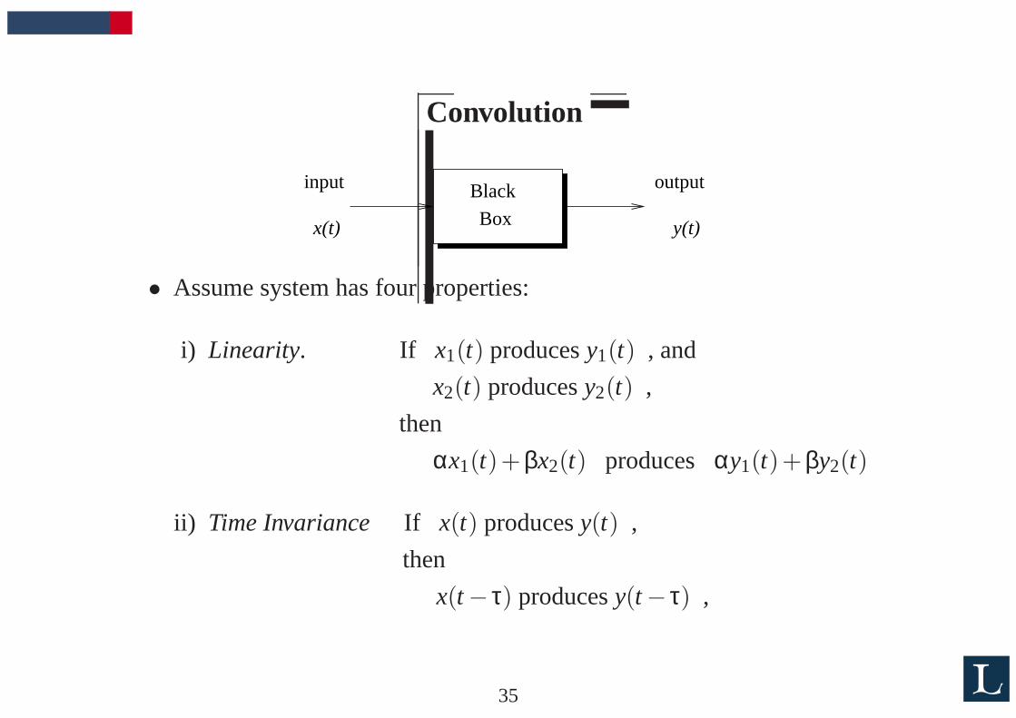
Convolution

Box

Blackinput output

x(t) y(t)

• Assume system has four properties:

i) Linearity. If x1(t) producesy1(t) , and

x2(t) producesy2(t) ,

then

αx1(t)+βx2(t) produces αy1(t)+βy2(t)

ii) Time Invariance If x(t) producesy(t) ,

then

x(t − τ) producesy(t − τ) ,

35

Convolution (cont.)

Box

Blackinput output

x(t) y(t)

iii) Continuity.continuous “small” changes in inputx(t), produce

continuous “small” changes in outputy(t)

iv) Causality.Outputy at timet does not depend on inputx at a time

later thant.

36

Convolution and Impulse Response

With these four conditions met we have:

• there exists ag(t) such that

y(t) =Z t

0x(λ)g(t −λ)dλ =

Z t

0x(t −λ)g(λ)dλ

• g(t) contains all the information about the system

⋄ g(t) is known as the system’s ”impulse response”

⋄ integral is known as the ”convolution integral”

37

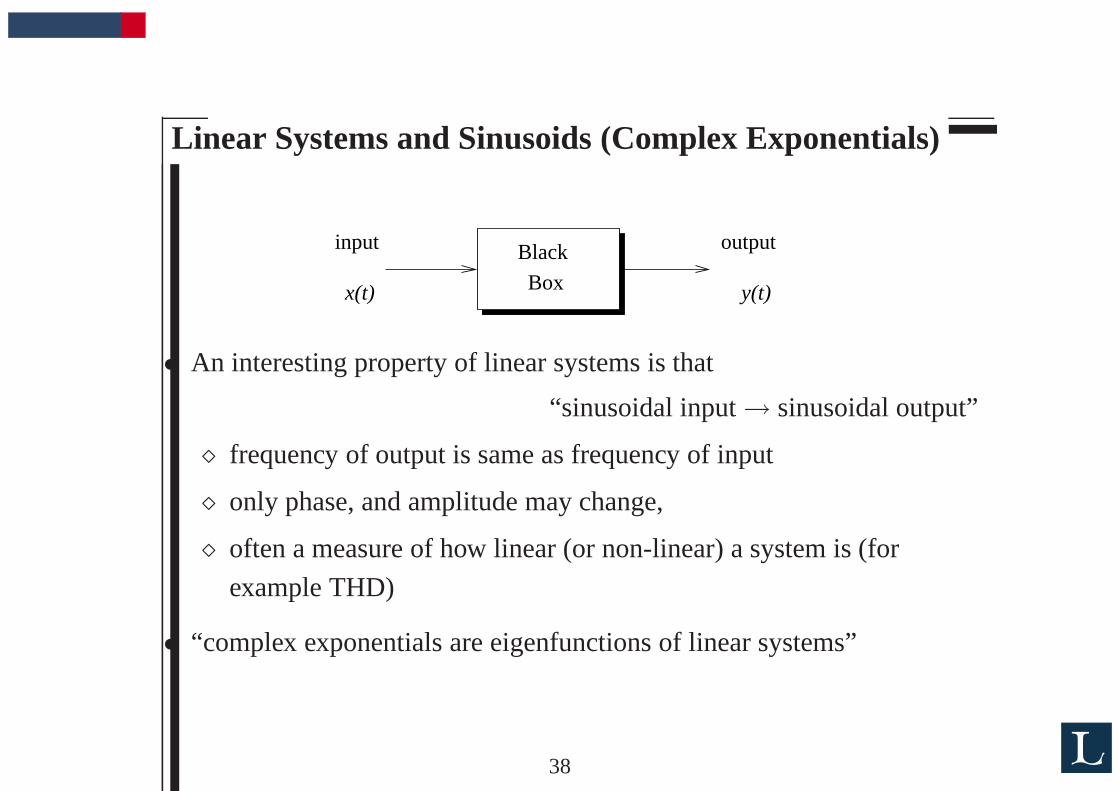
Linear Systems and Sinusoids (Complex Exponentials)

Box

Blackinput output

x(t) y(t)

• An interesting property of linear systems is that

“sinusoidal input→ sinusoidal output”

⋄ frequency of output is same as frequency of input

⋄ only phase, and amplitude may change,

⋄ often a measure of how linear (or non-linear) a system is (for

example THD)

• “complex exponentials are eigenfunctions of linear systems”

38

Z -Transform

• Consider the sequence an∞n=0

• form the summation, A(z) =∞

∑n=0

anz−1

wherez∈ C

• for thosez for which the sum converges we callA(z)

the “ Z -Transform ofan”.

• often considered analogous to the Laplace Transform for discrete

sequences

39

Fourier Series

40

Fourier Series

We return to Fourier’s solutions of the heat problem

x=0 x=π

Initial Conditions

f(x)=u(x,0)

u(0,t)=0 u( ,t)=0πBoundary Conditions

• Found solutions of form u(x, t) = bn e−n2t sinnx

• for initial conditions f (x) = u(x,0) =N

∑n=1

bnsinnx 0 < x < π

How general is this solution?

41

What functions can be created on[0,π] byN

∑n=1

bnsinnx ?

−1

0

1

−1

0

1

−1

0

1

−1

0

1

−1

0

1

−1

0

1

−1

0

1

−1

0

1

−1

0

1

b

b

b2

b1

3

4

Σ

42

More General Form

• Let’s shift from f (t) =N

∑n=1

bnsinnt on [0,π] ...

• ... to a more general form of

f (t) =∞

∑n=−∞

cneint =∞

∑n=−∞

cn (cosnt+ i sinnt) and extend over allt.

• Can ask similary question ...

What are the f(t) that can now be constructed?

• a bit of reflection yields thatf (t) will be periodicwith periodT = 2πf (t) = f (t +T)

• also noteZ

T=

Z π

−π=

Z 2π

0=

Z a+2π

afor anya∈ R

43

Relations

• Suppose f (t) =∞

∑n=−∞

cneint and also assume∞

∑n=−∞

|cn| < ∞

• ConsiderZ π

−πf (t)e−imtdt =

Z π

−π

(∞

∑n=−∞

cneint

)

e−imtdt

=

Z π

−π

∞

∑n=−∞

cne−i(n−m)tdt

=∞

∑n=−∞

cn

Z π

−πe−i(n−m)tdt

• Look atZ π

−πeiktdt =

2π k = 0

0 k 6= 0

• So, we haveZ π

−πf (t) e−imtdt = 2π cm

44

Obtaining cm from f (t)

• Interestingly, we now see that iff (t) =∞

∑n=−∞

cneint ...

• ... then we could find thecm from the integral

cm =12π

Z π

−πf (t) e−imtdt

45

Fourier Series, Definition

Def’n 4.1 Let f be a function with period 2π that is absolutely Riemann

integrable over a period.

Define the numberscn, with n∈ ZZ by

cn =12π

Z

Tf (t) e−intdt =

12π

Z π

−πf (t) e−intdt.

• cn are called “Fourier coefficients off ”

• The “Fourier Series off ” is the series ∑n∈ZZ

cneint

46

What about convergence?

• We’ve made no statement about if series converges.

• Even if the series converges, we’ve made no statement about what the

series converges to.

• Let’s play with this a bit in MATLAB

⋄ construct a vectort, and define some functionf (t)

⋄ calculatecn for f (t)

⋄ look at series for an increasing number of terms

47

Convergence of Fourier Series

• It certainly looks like the series∞

∑n=−∞

cneint is approximating (or

converging to)f (t) as # of terms increases.

⋄ What do we mean by convergence here?

⋄ What do we mean by approximation here?

• Much of Chapter 4 is dedicated to the details of the convergence

question.

48

End Result, Theorem 4.2

If

• f is a continuous onT,

• and its Fourier coefficientscn are such that∞

∑n=−∞

|cn| is convergent,

then the Fourier Series is

• convergent with sum= f (t) for all t ∈ T,

• and the convergence is uniform onT

49

Quite a remarkable path!

• Our original motivation was to see how general Fourier’s heat equation

solution was.

• Our investigation leads to the result that an extremely large class of

continuous, 2π periodic function could be constructed from complex

exponentials ( ∑n∈ZZ

cneint )

• We could say that we “build up” an arbitrary, continuous, 2π periodic

function by taking a “weighted sum” ofeint .

• This leads to the ideas of “bases” and “basis functions”

We investigate this tomorrow!

50

Day 2

51

Yesterday

• We could say that we “build up” an arbitrary, continuous, 2π periodic

function by taking a “weighted sum” ofeint .

• This leads to the ideas of “bases” and “basis functions”

• Why is this Fourier idea so big?

• What’s the fascination with these complex exponential functionseint?

52

Why are eint so important?

• Partial differential equations often have (damped) complex

exponentials as their solution.

• Mechanical systems oftenvibrateor resonatewith periodic

characteristics.

• Complex exponentials areeigenfunctionsof linear systems!

To explore more, we need to develop ideas, known as L2 Theory

53

Inner Product

Def’n 5.1 Let V be a complex vector space. An inner productonV is a

complex-valued function〈u,v〉 of u andv∈V having the following

properites:

• 〈u,v〉 = 〈v,u〉

• 〈αu+βv,w〉 = α〈u,w〉+β〈v,w〉

• 〈u,u〉 ≥ 0

• 〈u,u〉 = 0 ⇒ u = 0

54

Examples of an Inner Product

Example 5.3.Let C(a,b) be the set of continuous, complex-valuedfunctions defined on the compact interval[a,b] and set

〈 f ,g〉 =

Z b

af (x)g(x)dx.

This is an inner product.

Another Example Let u,v∈ C N (say, N-dimensional column vectors).Then,

〈u,v〉 = uT v = [u1 u2 . . .uN ]

v1

v2...

vN

=N

∑k=1

ukvk

55

Properties of Inner Product

Inner productions satisfy:

• |〈u,v〉| ≤ ‖u‖ ‖v‖ (Cauchy-Schwarz Inequality)

• |u+v| ≤ ‖u‖+‖v‖ (Triangle Inequality)

In a sense,

• inner products give us the idea of “distance”

• inner products define a “geometry”

56

Orthogonal Projections

Let φkNk=1 be an orthonormal set in the spaceV, and letu be an arbitrary

vector inV.

The orthogonal projection ofu on to the subspace ofV spanned byφkNk=1

is the vector,

PN(u) = 〈u,φ1〉 φ1 + 〈u,φ2〉 φ2 + . . .〈u,φN〉 φN

=N

∑k=1

〈u,φk〉︸ ︷︷ ︸

coeffs

φk︸︷︷︸

basis vector

57

Useful Theorem

Thm 5.2 If φ1, φ2, . . ., φN is an orthonormal basis in aN-dimensional inner

product spaceV. Then everyu∈V can be written as

u =N

∑j=1

〈u,φ j〉 φ j

and furthermore one has

‖u‖2 =N

∑j=1

|〈u,φ j〉|2

58

Crowning the Fourier System!

The two orthogonal systems

•

eint

n∈ ZZ

• cosnt,n≥ 0;sinnt,n≥ 1n

are each complete inL2(T).

Loosely, in other words, any square integrable,T-periodic function can be

constructed from these basis elements!

59

Back to the 1-D Wave equation

Consider a vibrating string

x=0 x=π

f(x)

u(0,t)=0 u( ,t)=0πBoundary Conditions

Initial Displacement

Initial Velocity

g(x)

• (E)∂2u∂x2 =

∂2u∂t2 Equation

• (B) u(0, t) = u(π, t) = 0 Boundary Conditions

• (I1) u(x,0) = f (x) Inital (Displacement) Conditions

• (I2)∂u(x,0)

∂t= g(x) Inital (Velocity) Conditions

60

1-D Wave equation, Vibrating String

x=0 x=π

f(x)

u(0,t)=0 u( ,t)=0πBoundary Conditions

Initial Displacement

Initial Velocity

g(x)

The same separation of variables techniques yields solution:

u(x, t) =∞

∑n=1

(ancosnt+bn sinnt)sinnx

• notice we have oscillations in time

• notice dependence also on position

61

Fourier Transform Definition

• Assumef is a function onR such thatZ ∞

−∞| f (t)| dt =

Z

R| f (t)| dt is convergent.

• define f (ω), for every realω as

f (ω) =

Z ∞

−∞f (t)e−iωt dt

• the function f (ω) is known as theFourier Transformof f (t).

• Often in engineering notationF(ω) is used instead of f (ω).

62

Linearity of the Fourier Transform

• The mappingF : f (t) 7→ f (ω) is linear

That is, withF [ f (t)] = f (ω) andF [g(t)] = g(ω),

then we haveF [α f (t)+βg(t)] = α f (ω)+β g(ω).

63

Invertibility of the Fourier Transform

• The mappingF : f (t) 7→ f (ω) can be inverted.

That is, withF [ f (t)] = f (ω),

there is an inverse mappingF −1[ f (ω)] = f (t).

• We have theInverse Fourier Transform

f (t) =12π

Z ∞

−∞f (ω)eiωt dω

64

The Discrete Fourier Transform

• Often we deal with sampled data

• Numerical computations require discrete data

• We need a Fourier Transform in these cases

⋄ a direct and obvious extension of Fourier Transform

65

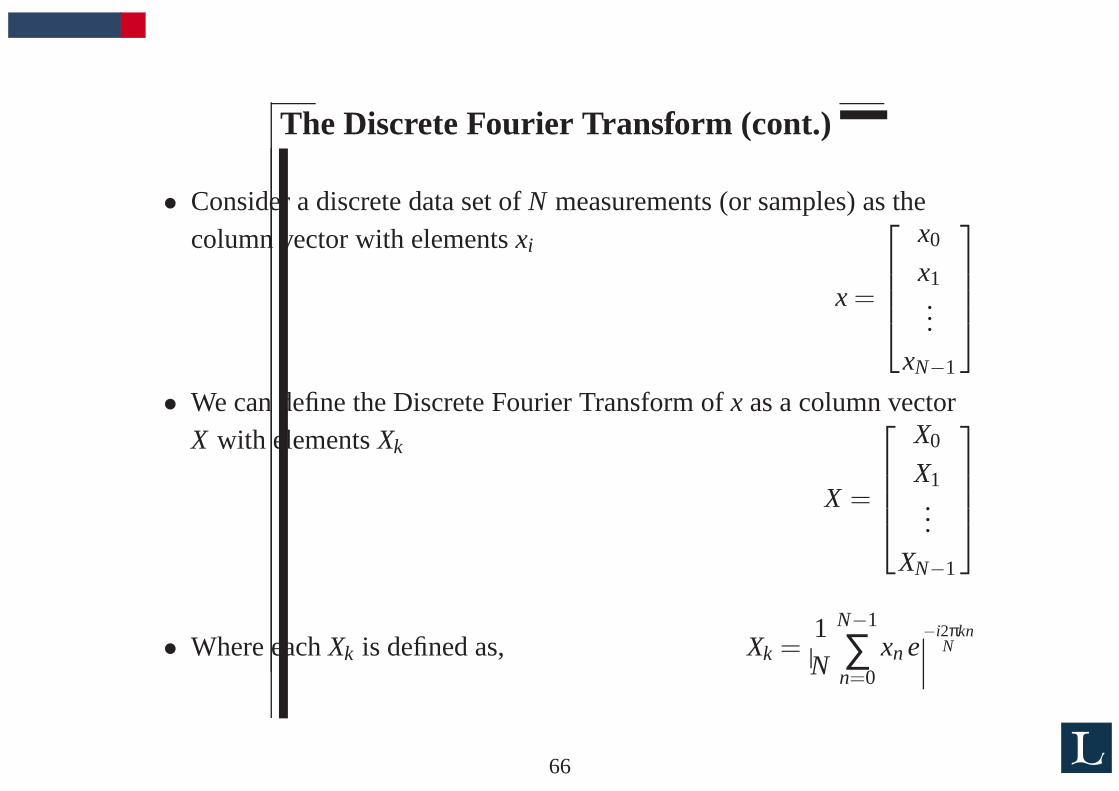
The Discrete Fourier Transform (cont.)

• Consider a discrete data set ofN measurements (or samples) as thecolumn vector with elementsxi

x =

x0

x1...

xN−1

• We can define the Discrete Fourier Transform ofx as a column vectorX with elementsXk

X =

X0

X1...

XN−1

• Where eachXk is defined as, Xk =1N

N−1

∑n=0

xn e−i2πkn

N

66

Discrete Fourier Transform & its Inverse

• Discrete Fourier Transform

Xk =1N

N−1

∑n=0

xn e−i2πkn

N

• Inverse Discrete Fourier Transform

xn =N−1

∑k=0

Xk ei2πkn

N

67

Discrete Fourier Transform as Inner Product

• Consider inner product〈x,φk〉• whereφk is thekth Fourier basis vector

φk =

ei2πk0

N

ei2πk1

N

...

ei2πk(N−1)

N

• We have then

Xk =1N〈x,φk〉 =

1N

[x0 x1 . . . xN−1 ]

e−i2πk0

N

e−i2πk1

N

...

e−i2πk(N−1)

N

=1N

N−1

∑n=0

xn e−i2πkn

N

68

Discrete Fourier Transform as Matrix Transformation

[X0 X1 . . . XN−1 ]

=1N

[x0 x1 . . . xN−1 ]

e−i2π·0·0

N e−i2π·1·0

N . . . e−i2π·(N−1)·0

N

e−i2π·0·1

N e−i2π·1·1

N . . . e−i2π·(N−1)·1

N

......

. . ....

e−i2π·0·(N−1)

N e−i2π·1·(N−1)

N . . . e−i2π·(N−1)·(N−1)

N

=1N

[x0 x1 . . . xN−1 ]

69

Discrete Fourier Transform as Coefficients and Basis

• Let φkN−1k=0 , be an orthonormal basis forV,

• then,u be an arbitrary vector inV, can be written as

u = 〈u,φ0〉φ0 + . . .+ 〈u,φN−1〉φN−1 =N−1

∑k=0

〈u,φk〉︸ ︷︷ ︸

coeffs

φk︸︷︷︸

basis vector

• re-interpret Discrete Fourier Transform in this way,

x = 〈x,φ0〉︸ ︷︷ ︸

X0

φ0 + 〈x,φ1〉︸ ︷︷ ︸

X1

φ1 + . . .+ 〈x,φN−1〉︸ ︷︷ ︸

XN−1

φN−1 =N−1

∑k=0

〈x,φk〉︸ ︷︷ ︸

coeffs

φk︸︷︷︸

basis vector

= x is a weighted sum of complex exponentials (sinusoids)

70

An Intuitive Approach

71

Music as a signal

• What is music?

• What is sound?

• What is a signal?

• How do we think about signals?

72

Music as a point in space!

• Let’s consider a piece of music as a point in space:

⋄ a high dimensional space

⋄ how could we describe this point in space?

⋄ where is it?

73

Describing Things

How do we describe things in general?

• Maybe we ...

⋄ describe the thing’s variouscomponents

⋄ then describe how these components areassembledto make the

thing.

... back to signals

• This is a useful concept for us in signals and systems

⋄ describe the signal by somecomponents (analysis)

⋄ describe how the signal isassembled (synthesis)

74

Describing Music/Signals

• maybe in your mind you think of a signal as thegraphof a function

such as:

t

f (t)

• ... but we think of a signal as apoint in a “high dimensional space”!

Why do this?

• gives a concept of “closeness”

• gives a geometry ...

• geometry blends mathematics withintuition

75

Point in Space = Vector

• Example, point in 3D

p p =

x

y

z

76

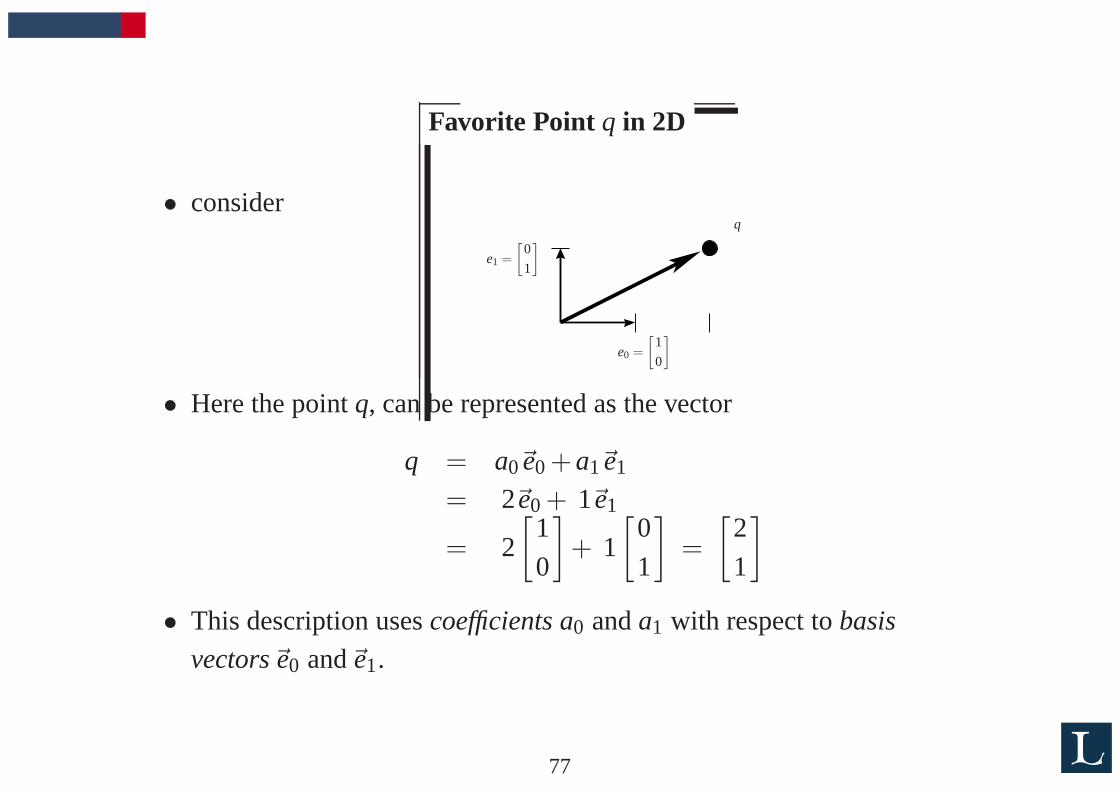
Favorite Point q in 2D

• considerq

e0 =

[1

0

]

e1 =

[0

1

]

• Here the pointq, can be represented as the vector

q = a0~e0 +a1~e1

= 2~e0 + 1~e1

= 2

[1

0

]

+ 1

[0

1

]

=

[2

1

]

• This description usescoefficients a0 anda1 with respect tobasis

vectors~e0 and~e1.

77

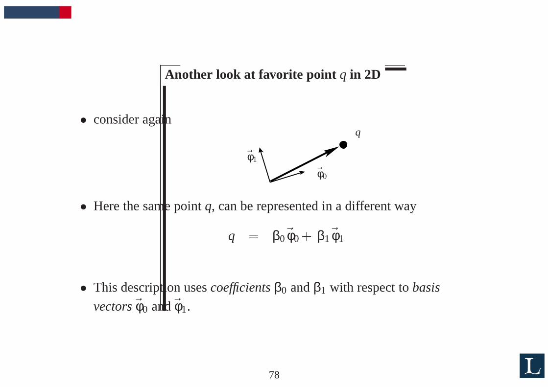
Another look at favorite point q in 2D

• consider againq

~φ0

~φ1

• Here the same pointq, can be represented in a different way

q = β0~φ0 + β1~φ1

• This description usescoefficientsβ0 andβ1 with respect tobasis

vectors~φ0 and~φ1.

78

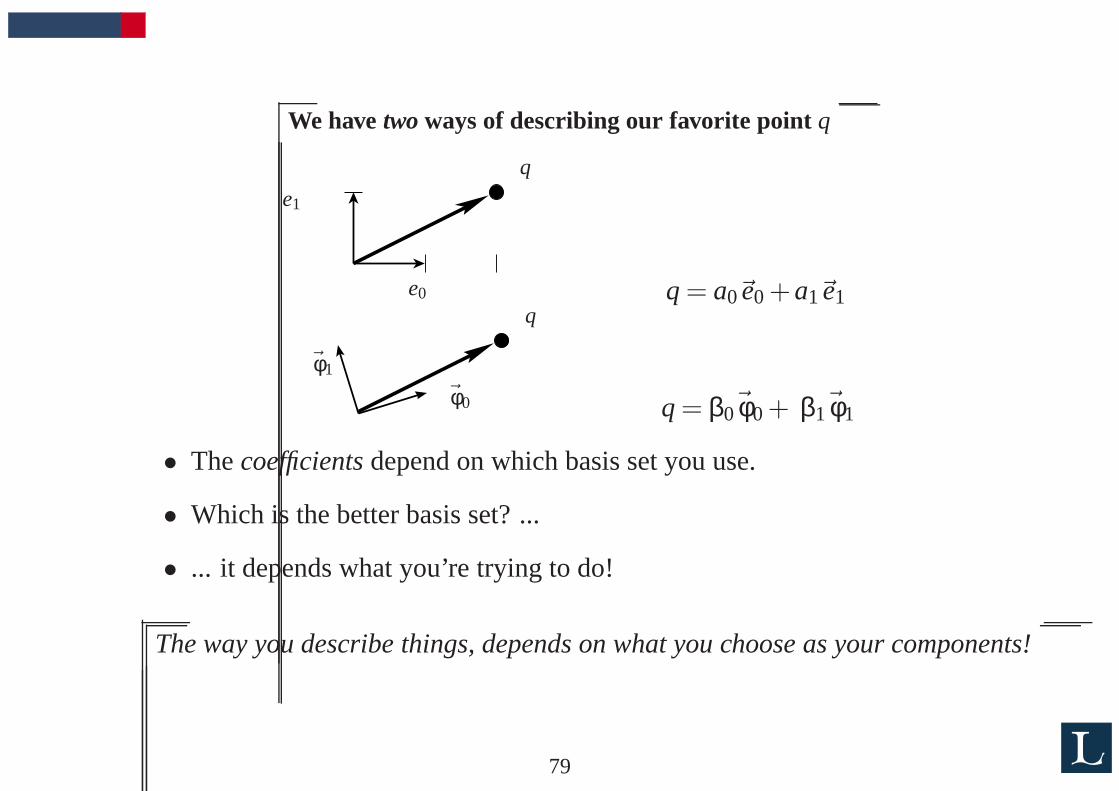
We havetwo ways of describing our favorite pointq

q

e0

e1

q = a0~e0 +a1~e1q

~φ0

~φ1

q = β0~φ0 + β1~φ1

• Thecoefficientsdepend on which basis set you use.

• Which is the better basis set? ...

• ... it depends what you’re trying to do!

The way you describe things, depends on what you choose as your components!

79

What does this have to do with Music?

• consider 10 seconds of CD-audio (samples of music)

• this is a discrete-time signal:x[0], x[1], . . ., x[440999]

• could think of as the vector (why?)

x =

x[0]

x[1]

. . .

x[440,999]

• this is a point in a 441,000 dimensional space

80

What does this have to do with Music? (cont.)

• We’ve seen the coefficients to describe a vector depend on thebasis

vectorset we choose.

• If we choose thetime samplesas the basis vectors we could represent

our music as

x = x[0]

1

0

0...

0

+ x[1]

0

1

0...

0

+ . . . + x[440,999]

0

0

0...

1

= x[0]~e0 + x[1]~e1 + . . . + x[440,999]~e440,999

• we have chosen adifferentbasis set, sayφ0,φ1, . . . ,φ440,999,,

81

What does this have to do with Music? (cont.)

• Remember the coefficients to describe a vector depend on thebasis

vectorset we choose.

• using the natural basis vectors (times samples)e0,e1, . . . ,e440,999,,

we have

x = x[0]~e0 + x[1]~e1 + . . . + x[440,999]~e440,999 =440,999

∑i=0

x[i]~ei

• using the basis vectorsφ0, φ1, . . . , φ440,999,, we have

x = β0~φ0 + β1~φ1 + . . . + β440,999~φ440,999 =440,999

∑i=0

βi~φi

• note: the coefficientsx[i] andβi would be different

82

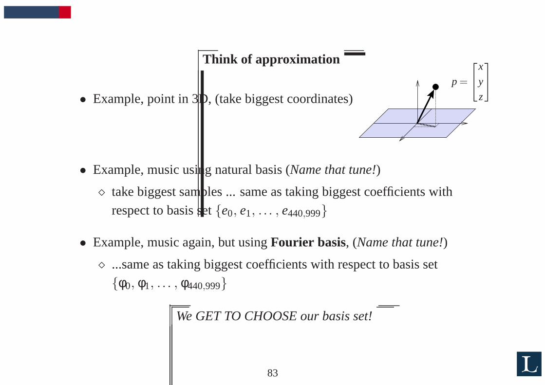
Think of approximation

• Example, point in 3D, (take biggest coordinates)p =

x

y

z

• Example, music using natural basis (Name that tune!)

⋄ take biggest samples ... same as taking biggest coefficientswithrespect to basis sete0, e1, . . . , e440,999

• Example, music again, but usingFourier basis, (Name that tune!)

⋄ ...same as taking biggest coefficients with respect to basissetφ0, φ1, . . . , φ440,999

We GET TO CHOOSE our basis set!

83

Name that tune!

• The idea of the game: I give you a partial description of song,you tryto guess what song it is

• One way to play: I give you a partial description in the time domain:

⋄ the biggest time-sample

⋄ the 10 biggest time-samples

⋄ the 100 biggest time-samples ...

• Another way: I give you a partial description in the frequency domain:

⋄ the biggest sine wave component

⋄ the 10 biggest sine wave components

⋄ the 100 biggest sine wave components ...

84

Not just used for sounds...but IMAGES too!

85

Not just used for sounds...but IMAGES too!

86

Not just used for sounds...but IMAGES too!

87

Not just used for sounds...but IMAGES too!

88

Points in Space: 2-D

• Given a vector in 2D and a orthonormal set of basis vectors~φ0 and~φ1,how do we find the coordinates?

• Given~q = 2~e0 +1~e1, what are coordinates of~q w. r. t. basis~φ0,~φ1 ?

• for the case~e0 =

[1

0

]

,~e1 =

[0

1

]

,~φ0 =

[1√2

1√2

]

, and~φ1 =

[ −1√2

1√2

]

it looks

like this

−2 −1.5 −1 −0.5 0 0.5 1 1.5 2

−2

−1.5

−1

−0.5

0

0.5

1

1.5

2

q

~e0

~e1~φ0~φ1

89

Finding the coefficients (ii )

−2 −1.5 −1 −0.5 0 0.5 1 1.5 2

−2

−1.5

−1

−0.5

0

0.5

1

1.5

2

q

~e0

~e1 ~φ0~φ1

• Usedot product(also known asinner product)

• Given~q = 2~e0 +1~e1 =

[2

1

]

, we seekβ0 andβ1, such that

~q = β0~φ0 +β1~φ1.

β0 = ~q· ~φ0 =~qT ~φ0 = [2 1]

[1√2

1√2

]

=3√2≈ 2.12

β1 = ~q· ~φ1 =~qT ~φ1 = [2 1]

[ −1√2

1√2

]

=−1√

2≈ 0.707

90

Inner product ( i)

• to find coefficientβ0, took inner product of~q with basis vector~φ0.

β0 = ~q· ~φ0 =~qT ~φ0 = [2 1]

[1√2

1√2

]

=1

∑i=0

q(i)φ0(i)

• if our vector instead lived in inN dimensions? Concept is the same...

β0 = ~q· ~φ0 =N−1

∑i=0

q(i)φ0(i)

• If our vector wasinfinite dimensional...concept is the same

β0 = ~q· ~φ0 =∞

∑i=0

q(i)φ0(i)

• If our vector wasinfinite dimensionaland defined on interval 0< t < T

...concept is the same

β0 = ~q· ~φ0 =Z T

0q(t)φ0(t)dt

91

Fourier Transform is same Concept!

• The Fourier Transform can be used to represent

• Fourier Transform uses the orthog basis “vectors” over−∞ < t < ∞

⋄ ejωt = cos(ωt)+ i sin(ωt)

• Fourier Transform “coefficients” found by inner products

X(ω) =Z ∞

−∞x(t)e−iωtdt

= F x(t)

92

Fourier Transform

• Let’s us think either in frequency domain or time domain

• Fourier Transform: X(ω) = F x(t)

• Inverse Fourier Transform: x(t) = F −1X(ω)

• Fourier Transform Pair: x(t)F↔ X(ω)

93

An Audio Example

• Look at the Fourier Transform of 7 seconds audio shown below:

0 0.2 0.4 0.6 0.8 1 1.2 1.4 1.6 1.8 20

0.2

0.4

0.6

0.8

1

Normalized Frequency

|X|

• Can you “see” how it should sound?

⋄ it’s a bit of a problem

⋄ we see how much of each sinusoid (each 7 seconds long) is neededto make the audio...

... but that’s not how we (as humans) interpret the sound!

94

Variation on the Theme

Frequency content over a shorter period of time.

• Why not segment the audio into short time frames?

• Perform the FFT analysis on each short segment

• This is called theperiodogram

Create an image by

• Placing each FFT vertically

• Encode large|X| values as “hot”

• Can now see evolution of spectra, as time progesses

95

Audio Example Revisited

• A Periodogram of our audio signal

2000

4000

6000

8000

10000

12000

14000

16000

time (Sec)

freq

(H

z)

0 1 2 3 4 5 6 70

200

400

600

800

1000

1200

1400

1600

1800

2000

• What can we understand about signal now?

• Let’s listen to it!

96

Periodogram

• By segmenting our data, we can “see” time evolution of the spectra.

• We obtained this new capability by:

⋄ moving away from using a set of “global basis function” (defined

over the time duration of the signal)...

⋄ ... to a set of basis functions that are active only in “local regions”

97

This periodogram leads to ideas found in wavelets

• Wavelets are an analysis of signals (functions)

⋄ where the basis functions have compact support

⋄ have particular scaling properties

You’ll be seeing wavelets with Niklas Grip in the next coursesection

Thanks for your attention!

98