TitleSIMPLE EVALUATION METHODS FOR ROADPAVEMENT MANAGEMENT IN DEVELOPINGCOUNTRY( Dissertation_全文 )

Author(s) Heng Salpisoth

Citation Kyoto University (京都大学)

Issue Date 2014-03-24

URL https://doi.org/10.14989/doctor.k18249

Right

Type Thesis or Dissertation

Textversion ETD

Kyoto University

SIMPLE EVALUATION METHODS FOR

ROAD PAVEMENT MANAGEMENT

IN DEVELOPING COUNTRY

HENG SALPISOTH

2014

SIMPLE EVALUATION METHODS FOR

ROAD PAVEMENT MANAGEMENT

IN DEVELOPING COUNTRY

by

HENG SALPISOTH

March 2014

A dissertation submitted to

Graduate school of engineering, Kyoto University

In partial fulfillment of requirements for the degree of

Doctor of Engineering

i

ABSTRACT

Pavement Management System (PMS) does very important roles in pavement

maintenance and management to provide a comfortable and safety pavement to the people

and vehicles travelling on it. However, there still have been many challenges in PMS

occurred in both developed and developing countries. The challenges are related to

inspection, database, management cycle, pavement deterioration forecasting, Life Cycle

Cost Analysis (LCCA), accounting by optimization procedures, and even political issues.

In this study, among the above challenges two main challenges are focused and discussed.

One is how to predict pavement performance with appropriate models using the

incomplete data in order to make optimal maintenance and repair strategies. The other is

how to monitor and evaluate pavement condition regularly and frequently in routine

inspection in a developing country that faces extreme limitation of budget. In this study,

the following factors and issues are discussed.

First, several prediction models were examined using actual but limited information

about pavements, to find optimum model for developing countries. Actual data of IRI

(International Roughness Index), FWD (Falling Weight Deflectometer) deflections and

traffic volume measured in all 1-Digit national roads of Cambodia were used to build the

models and the models were examined using those data of national road No.5. And it was

found that the increase in roughness of pavement is related strongly to the state of

roughness itself, and also the prediction model using exponential function proposed by

the author exhibits most accurate prediction among the conventional models under

limited information.

Next, a simple method for structural evaluation of asphalt pavement based on impact

sound as well as impact force was proposed. Characteristics of impact force and impact

sound were investigated on model pavement, and it was found that peak frequencies are

related to the subgrade elasticity, and that the impedance of a impact force has linear

relationship with the averaged elasticity from the surface to some depth. Then, on the

basis of parametric analysis using FEM analysis, it was also found that the square root of

elasticity of subgrade has linear relationship with peak frequencies. Thus it can be said

that simple evaluation can be attained by combing the analyses of impact sound and

impact force.

Thirdly, a simple system for IRI estimation using motor bicycle was developed.

Herein the characteristics of five kinds of motor bicycles were examined by hump

calibration test to investigate their impulse response. Then, IRI estimation was conducted

by the responses of front and rear sprung and those of mass unsprung. It was found that

ii

the responses of front sprung mass is most adequate to estimate IRI.

Finally, a simple method of actual live load evaluation was studied on the basis of

current traffic data by Bridge Weigh-In-Motion in Bangkok city, Thailand. It was

confirmed that this simple Bridge Weigh-In-Motion system can be applied even in

Thailand, and found that the obtained daily five tons conversion axles number is

slightly less than that of AASHTO standard axles loading. In this case, model load was

almost equal to actual load but when overloaded vehicles are detected, actual load must

be monitored as a double load yields 16 times as large fatigue damage.

iii

ACKNOWLEDGMENTS

I would like to express my sincerest appreciation and thanks to my supervisor, Professor

Hirotaka KAWANO, for giving me the opportunity to continue my studies and research in

his laboratory. His continued guidance, his kindness, his accessibility and his support

have motivated me through my academic endeavors. Through his invaluable counsel, I

have learned a great deal from him in both academic and personal life. All these are most

deeply appreciated.

The same appreciation and my special thanks go to Associate Professor Yoshinobu

OSHIMA who is also my advisor and mentor throughout my studies. I am sincerely

grateful to him for the opportunity he has given me to research this exciting topic. I really

and strongly appreciate his inspiration, encouragement, patience, assistance and his

invaluable guidance, which play an important role in the completion of this dissertation.

Many thanks are also due to Associate Professor Atsushi HATTORI, Assistant

Professor Toshiyuki ISHIKAWA, Assistant Professor Hiroshi HATTORI, my senior Dr.

Kyosuke YAMAMOTO, Secretary Noriko INADA, Secretary Sonomi MATSUKAWA,

and all the members in the KAWANO Structures Management Engineering Laboratory,

for their helpful assistance and great contribution in my research studies.

I wish to strongly and gratefully acknowledge the assistance of Cambodia JICA

Expert Mr. Tsuyoshi KUBOTA, Mr. Tadao KUWANO, and JICA staffs concerned for

their help in supporting Cambodian road network data. My great thanks also go to Prof.

NAGAYAMA, the University of Tokyo, for providing VIMS system in this research. This

research was also strongly supported by Mr. Taro HOMMA, MEISEI KENSETSU

INDUSTRY CO., LTD, I really appreciate for his contribution.

I wish also to extend my genuine thanks and my deepest affection to all seniors,

juniors, and friends that I cannot write all here, for their kindness, their support and their

great friendship during my studied life.

Lastly, I would like to express my deepest gratefulness and highest respect to my

parents and brothers for their endless love and support. Without their encouragement,

especially my father, I would never have embarked on this endeavor, and the

accomplishment of my study would not have been possible.

iv

v

TABLE OF CONTENTS

Chapter 1 Introduction 1

1.1 General remarks on a road pavement management system 1

1.2 Overview of road pavements in developing countries 3

1.3 Previous studies on road pavement evaluations 5

1.3.1 Live load evaluation 5

1.3.2 Condition evaluation of road pavements 7

1.3.3 Deterioration prediction of road pavements 21

1.4 A simple management system for road pavements in developing countries 25

1.5 Objective and scopes 28

Chapter 2 Evaluation of IRI prediction models 31 with limited information

2.1 General remarks 31

2.2 General outline of this chapter 32

2.2.1 Survey data 32

2.2.2 Transition of IRI 32

2.2.3 Relationship between IRI increment and influential factors 35

2.3 IRI prediction models 37

2.3.1 HDM-4 and LTPP model 37

2.3.2 Exponential equation model 38

2.3.3 Neural network model 40

2.3.4 Markov model 43

2.3.5 Comparison of prediction models 48

2.4 Summary 49

vi

Chapter 3 Development of an evaluation system of 51 pavement structures based on impact testing

3.1 General remarks 51

3.2 Impact test on model pavements 53

3.2.1 Model pavements 53

3.2.2 Outline of each test 55

3.2.3 Results and discussions 57

3.3 Parametric analysis for impact sound using FEM 64

3.3.1 Outline of FEM and model analysis 64

3.3.2 Verification of the numerical model 66

3.3.3 Effect of each layer thickness on dominant frequency 66

3.3.4 Effect of each layer elastic modulus on dominant frequency 71

3.4 Evaluation procedure of pavement structures 73

3.5 Summary 74

Chapter 4 Development of a simple IRI measurement system 75 using a motor bicycle for roughness evaluation

4.1 General remarks 75

4.2 Measurement principle 75

4.2.1 VIMS (Vehicle Intelligent Monitoring System) 75

4.2.2 Principle of IRI estimation using a motor bicycle 79

4.3 Measurement test 80

4.3.1 Measurement outline 80

4.3.2 Hump test 82

4.3.3 Running test 83

4.4 Measurement results 84

4.4.1 Hump test results 84

4.4.2 Running test results 92

4.5 Summary 95

vii

Chapter 5 Evaluation of actual live loads using 97 a Bridge Weigh-In-Motion technique

5.1 General remarks 97

5.2 Bridge Weigh-In-Motion 98

5.2.1 Principle of Bridge WIM 98

5.2.2 Monitored Bridge 100

5.2.3 Sensor location on pre-cast concrete slab 101

5.2.4 Calibration 103

5.3 Results of Bridge WIM 104

5.4 Comparison of actual and design load affecting fatigue deterioration 107

of road pavement

5.4.1 Daily five tons conversion axles number 107

5.4.2 Daily five tons conversion axles number for road pavement 108

deterioration evaluation in Bangkok city

5.5 Summary 109

Chapter 6 Conclusions 111

References 115

Appendixes

A.1 Road structures in developing countries A-1

A.2 Road structures evaluations A-1

viii

1

Chapter 1 Introduction

1.1 General remarks on a road pavement management system

In many developing countries of Asia and Africa, a pavement by asphalt tends to

deteriorate faster than expected comparing with that of developed countries, not only due

to low quality control during construction but due to improper maintenance after in

service. A pavement, one of most important infrastructures, is required to provide the

comfortable and safety to the people and vehicles travelling on it. However, a pavement is

a kind of consumable material and must be replaced at adequate timing because it is

easily and directly damaged or deteriorated by the applying load and surrounding

environment such as heavy traffic, intemperate climate and so on, which depends on its

location. Thus, for proper maintenance, first, it is necessary to examine and clarify the

factors of that deterioration. Then, monitoring and evaluating of the condition of

pavement should be done periodically to secure its performance for road network

maintenance and management.

Recently, infrastructure asset management has been a sensitive topic for civil

engineers. Even in developed countries, the budget invested in public work tends to

decrease although the aged structures to be maintained dramatically have increased, and

those structures must be maintained within that limited budget. A large number of

researches related to infrastructure asset management have been disseminated[1],[2],[3].

According to Kobayashi[4], the infrastructure asset management is “the optimal allocation

of the scare budget between the new arrangement of infrastructure and

rehabilitation/maintenance of the existing infrastructure to maximize the value of the

stock of infrastructure and to realize the maximum outcomes for the citizens”. Kobayashi

has applied this concept to the road and pavement sector.

In order to facilitate maintenance activities and also enhancing cost-effectiveness of

limited budget in pavement management, Pavement Management System (PMS)[5] has

been developed as a supporting system. PMS is a system considering life-cycle of

pavement including prospective study, design, construction and repair, and as evaluating

and predicting the condition of pavement, it provide a strategy minimizing the life-cycle

cost. In AASHTO guide for design of pavement structures[6], they describe PMS as “In a

broad sense of pavement management, it includes all actions and behaviors associated

with planning, design, construction, maintenance, evaluation, rehabilitation of pavement

sector in public work. PMS is a method or a tool to find out the best policy for agency to

2

provide, evaluate and maintain in the condition of offering services period. The

performance of PMS is to optimize the decision-making and feedback by predicting and

evaluating the result, by adjusting the work in the project period, the decision of different

project level can be integrated”. For example, the purpose of HDM-4 (Highway

Development and Management) system[8] is to reduce life-cycle cost of road pavement

that is suitable with project level and or network level, and include all activities of

pavement life-cycle.

Like this manner, many researchers as well as stake holders have mentioned that the

PMS does very important roles in pavement maintenance and management , but there are

many challenges in PMS remaining in both developed countries and developing countries.

The challenges are related to inspection, database, management cycle, pavement

deterioration forecasting, Life Cycle Cost Analysis (LCCA), accounting by optimization

procedures, and even political issues.

Among the above challenges, two main challenges are focused and discussed in this

study. One challenge is how to predict pavement performance with appropriate models

but using incomplete data in order to make optimal maintenance and repair strategies. The

other challenge is how to monitor and evaluate pavement condition regularly and

frequently in routine inspection with limited budget.

Generally, to evaluate asphalt pavement after in service, functional deterioration such

as topical cracking, deformation, wear, and low bearing of each layer or some such

structural deterioration were considered[7]. In many developing countries, associated with

road management system recommended from supporting countries, road surface

evaluation systems and structural evaluation systems have been applied[8]. In these

systems, visual inspection is conducted to the visual items such as crack, potholes and so

on, specialized measurement system equipped in a survey vehicle is used to evaluate the

evenness and deflection that need quantitative evaluation.

For example in Cambodia, by supporting by the World Bank, road asset management

has been conducted by using HDM-4 (Highway Development and Management) system[8].

Besides visual inspection once a year, road surface condition evaluation once a year using

IRI (International Roughness Index) and structural pavement evaluation once in two years

using FWD (Falling Weight Deflectometer) system have been done to collect the input

factors in HDM-4 system. However, as there are no enough budgets for maintenance

system, all the input factors are not collected: to run the above system requires much

budget. For instance, it takes long time to measure IRI and FWD deflection. Additionally,

it needs much cost to operate the system as it employs the specific vehicles and software.

When the measurement system is broken, periodical inspection should be postponed

because the repair of such system needs much money and time, and sometimes it is

required to import new parts. Additionally, not so many systems can be purchased due to

3

high cost to cover hole the country, and more than half a year is required to measure IRI

and more than one year is required to measure FWD deflection of all Cambodian road

networks.

Therefore, in developing country that does not have much maintenance budget, a

simple evaluation method with acceptable accuracy and low cost using simple device is

required to ensure pavement performance. By applying simple method without

large-scale measurement devices, measurement cost as well as measurement time can be

reduced, and the proper measurement can be done for pavement condition evaluation.

And also because of its simplicity, the owners or road agencies themselves could manage

the inspection easily, and any trouble in measurement such as disoperation may be also

avoided.

1.2 Overview of road pavements in developing countries

There are many kinds of pavement type employed in developing country, typically AC

(Asphalt Concrete) pavement, DBST (Double Bituminous Surface Treatment) pavement,

concrete pavement, laterite and earth. In the case of Cambodian road pavement[10] that is

managed by MPWT (Ministry of Public Works and Transport), AC pavement is about

930km, DBST pavement is about 3410km, concrete pavement is about 23km, laterite is

about 6045km and earth is about 1510km. Note that the structure of pavement consists of

selected sub-grade, laterite sub-base, aggregate base-course, herein just small amount of

cement stabilized base-course are used in the road network, and the surface with AC layer,

DBST layer or concrete layer. In addition, within about 2115km of national road, DBST

pavement occupies more than 65% of all pavement types. And also the same trend can be

found in other developing countries[11]. Therefore, it is clearly shown that most pavements

adopted in developing country are DBST pavement. Fig. 1-1 shows an example of DBST

pavement paved on Cambodian national road no.5.

From the user's guide of DBST[9], they describe DBST as a common type of pavement

surfacing construction which involves two applications of asphalt binder material and

mineral aggregate, usually less than 19mm thick, placed on a prepared surface. The

asphalt binder material is applied by a pressure distributor, followed immediately by an

application of mineral aggregate, and finished by rolling. The process is repeated for the

second application of asphalt binder material and mineral aggregate. The first application

of aggregate is coarser than the aggregate used in the second application and usually

determines the pavement thickness. The maximum size of mineral aggregate used in the

second application is about one-half that of the first.

4

Primarily, DBST is used for surfacing roads and streets, parking areas, open storage

areas, and airfield shoulders and overruns. DBSTs are also applied to base courses, new

pavements, recycled pavements, and worn or aged asphalt pavements. Furthermore,

DBSTs resist traffic abrasion and provide a water-resistant wearing cover over the

underlying pavement structure. Note that DBSTs add no structural strength to the existing

pavement, for this reason, it is not normally taken into account when determining the

structural thickness of the pavement. So generally, DBSTs are recommended for use on

primed non-asphalt bases, asphalt base course, or any type of existing pavement. They

provide a low cost nearly waterproof, wear-resistant surface that performs well under

medium and low volumes of traffic. This type of surface treatment is also useful as a

temporary cover for a new base course that is to be carried through a winter, or for a

wearing surface on base courses in planed stage construction.

DBST is in itself basically considered a maintenance activity. Surface treatments can

last for a considerable time provided they are designed and constructed properly. Surface

treatments under light to medium traffic may perform well for 7 to 10 years. So it is

necessary to monitor and measure the performance of the DBST by making periodic

inspections of the surface for signs of distress. Typical surface treatment distresses

include loss of cover aggregate, cracking, and bleeding. Anyway, all of distress modes in

pavement maintenance can be considered as surfacing distress due to cracking, raveling,

potholing and edge-break, deformation distress due to rutting and roughness, pavement

surface texture distress due to texture depth and skid resistance, and finally drainage

distress due to drainage. Thus, it is known that there have many defects of pavement to be

treated, however these defects are not independent but they have an effect on each other

due to their interaction mechanisms. For example, the roughness of pavement is widely

related to the structure of pavement, cracking, rutting, potholing, patching and also the

environment surrounding. By the way, potholes are caused by cracking, raveling and

enlargement, and the progression of pothole is affected by the time lapse between the

occurrence and patching of potholes. For the progression of edge break, it is caused by

loss of surface, and possibly base materials from the edge of the pavement. Commonly, it

arises on narrow roads with unsealed shoulders. An example of the deterioration of DBST

pavement is shown in Fig. 1-2. More details about deterioration condition and typical

deterioration of DBST can be found in reference [12], [13].

Basically, road deterioration depends on many factors such as original design,

material types, construction quality, traffic volume and axle loading, road geometry and

alignment, pavement age, environmental conditions and maintenance policy. Among

these factors, together with construction quality that is still an issue in developing country,

loading of traffic is also a serious problem. As the economic grows rapidly in developing

country, the problem of overload cannot be ignored[14],[15],[16]. And road pavement was

5

Fig. 1-1 DBST pavement of Cambodian

national road no.5

Fig. 1-2 Deterioration of DBST

pavement

deteriorated significantly by the effect of overload. One more important factor is

environmental conditions. We know that the climate of each area is different, so the

deterioration progress of pavement that is sensitive with temperature as well as

precipitation is also different. Moreover, the pavement can be damaged easily by local

disasters such as flood. Consequently from the above description, it is shown that in

developing country, not only the structure of pavement but also deterioration condition as

well as its influence factors is peculiar.

1.3 Previous studies on road pavement evaluations

1.3.1 Live load evaluation

Many Asian countries have been growing rapidly and expanded their possibility in

economics for recent years. Associated with this growth, infrastructures such as bridge,

tunnel and highway were needed, and those structures have been built by means of

foreign aids or by themselves. Roads and bridges must be designed to match their

performance to the requirements, and their bearing capacities are expected to resist the

design loads. In reality, however, unexpected overloads are applying to the bridges and

roads, and the overloads transcend their limitation because the trucks try to carry the

loads as much as possible (sometimes almost impossible) to increase their transport

efficiency. Such overloaded vehicles are often found in Asian countries and officially they

are not allowed by the regulation. In some cases, overloaded vehicles are unofficially

permitted by the police officers who do not understand its seriously harmful effect on

6

infrastructures. Mostly overloaded vehicles move over the structures at night when the

police officers are not in service.

In addition to this serious situation, sometimes live load model itself is not adequate

for the current situation because the assumed live load in design does not agree with the

actual loads. As is often the case in Asian countries, AASHTO (American Association of

State Highway and Transportation Officials), AUSROADS, EUROCODE and other

dominant codes are sometimes adopted for the design of infrastructures. These codes

have been applied by modifying their design loads but sometimes the traffic data is not

available or, even if the data is available it does not reflect the current situation because

the traffic investigation was done before their economic development.

In the case of Thailand, mainly they have adopted the codes according to AASHO: the

design loads are modified to match the actual situation in Thailand, on the basis of the

fundamental vehicle models in AASHTO. However, the traffic investigation on current

weights of vehicles in nationwide scale has been seldom conducted. Heng et al. [62]

conducted the traffic monitoring using Bridge Weigh-In-Motion (BWIM) and confirmed

that the BWIM system can be applied even in Thailand, and that the proposed load model

was slightly lower than H20 loading of AASHTO[62]. The details of this topic will be

discussed in Chapter 5.

In the case of Cambodia, overloaded vehicle is a serious problem for road

infrastructures. For bridges maintenance, AASHTO recommends the LRFR (Load and

Resistance Factored Rating) live load factor to be used for evaluating the existing bridges.

Surely AASTHO specification is often adopted in many Asian countries, but design live

loads may not be adequate to actual situation. Heng et al. [63] evaluated the live load in

Cambodia using the concept of LRFR live load factor which is used for bridge rating in

the United States. In their study, on the basis of Weigh-in-Motion data in Cambodia, the

factors were calibrated using the same statistical methods as in the original development

of LRFR. Accordingly, it was found that the traffic environment can be assessed by the

obtained factor and the factors in some area are beyond the standard values in LRFR.

They finally pointed out that proper live load model should be proposed in Cambodia[63].

In general it is difficult to grasp the real traffic loads of each road in different region.

In developing country, traffic loads are basically surveyed by weigh in motion station[20].

But because it requires a specific equipment and too high cost to manage the facilities,

and additionally, repairing cost is also high when it is in failure, a stable observation

cannot be attained. Thus, Bridge Weigh-In-Motion (B-WIM) system has been proposed

and applied to many places in developed countries. The principle and the application of

Bridge WIM will describe in Chapter 5. Because this system uses an existing bridge, it

can be applied to developing counties. Note that more simple observation could be

realized when the system is applied to culverts which are frequently used for road facility

7

in developing countries[10] instead of bridges. However, the possibility of this application

should be examined and studied in the future.

Even in developed countries, sometimes live load model may not match the actual

situation. Heng et al. [68] applied the B-WIM to national road in Japan to clarify the actual

condition. In their research, one year observation of traffic was done by B-WIM system.

In their system, two methods of axle detector using deck’s response and weight estimation

using the response of main girder were applied. More details about the system and

estimation result can be found in reference [64] ~ [68].

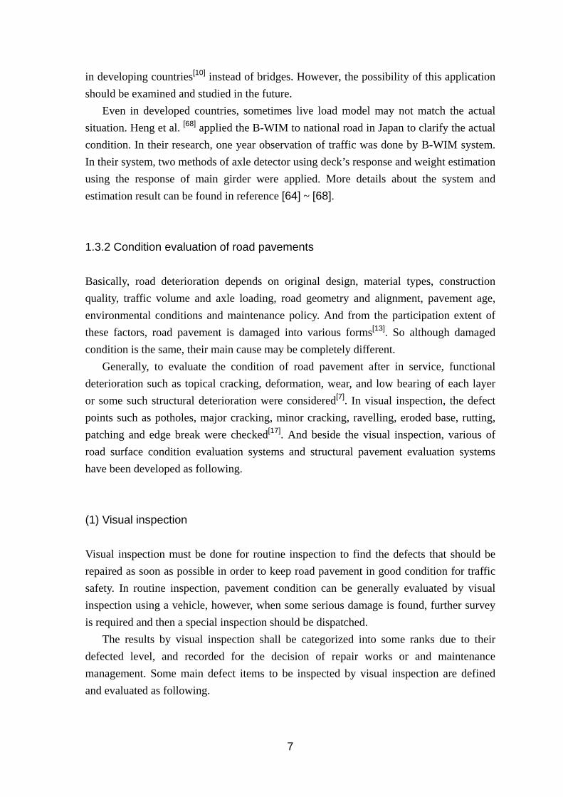
1.3.2 Condition evaluation of road pavements

Basically, road deterioration depends on original design, material types, construction

quality, traffic volume and axle loading, road geometry and alignment, pavement age,

environmental conditions and maintenance policy. And from the participation extent of

these factors, road pavement is damaged into various forms[13]. So although damaged

condition is the same, their main cause may be completely different.

Generally, to evaluate the condition of road pavement after in service, functional

deterioration such as topical cracking, deformation, wear, and low bearing of each layer

or some such structural deterioration were considered[7]. In visual inspection, the defect

points such as potholes, major cracking, minor cracking, ravelling, eroded base, rutting,

patching and edge break were checked[17]. And beside the visual inspection, various of

road surface condition evaluation systems and structural pavement evaluation systems

have been developed as following.

(1) Visual inspection

Visual inspection must be done for routine inspection to find the defects that should be

repaired as soon as possible in order to keep road pavement in good condition for traffic

safety. In routine inspection, pavement condition can be generally evaluated by visual

inspection using a vehicle, however, when some serious damage is found, further survey

is required and then a special inspection should be dispatched.

The results by visual inspection shall be categorized into some ranks due to their

defected level, and recorded for the decision of repair works or and maintenance

management. Some main defect items to be inspected by visual inspection are defined

and evaluated as following.

8

Potholes: bowl shaped hole of various size in the pavement surface, should be

evaluated by its number and its size.

Cracks: thin space generated by pavement breaking, should be evaluated by its width

its area.

Local aggregate loss: removal of aggregate from a surface dressing, or from surfacing

with coated aggregate, should be evaluated by its width and its length.

Edge break: pavement edge breakage or erosion, should be evaluated by its width and

its length.

Scratches: pavement surface cut by vehicle running, should be evaluated by its

length.

Bleeding: excess binder on the surface of the pavement, should be evaluated by its

width and its length.

(2) Road pavement structure evaluation

In order to evaluate pavement structure, there have a method using non-destructive test

instruments and a method investigate each layer of pavement by excavation[7]. The

excavation investigation is suited to investigate partially the details of structural pavement

condition however it is difficult to obtain the results of many investigation sections as it

requires much of labors and times. For non-destructive test instruments, there are some

devices measured deflection such as FWD (Falling Weight Deflectometer) (see Fig. 1-4)

and Benkelman beam (see Fig. 1-3(a)), and also some devices of flat plate loading test

equipment (see Fig. 1-3(b)). As Benkelman beam and flat plate loading test equipment

are used to investigate at the surface of base course and subgrade, so FWD is widely used

to evaluate nondestructively the structure of each pavement layer at the surface course.

Beside these instruments, Matsui et al.[18] have studied on theoretical approach of

surface wave method to evaluate the structure of pavement. They have compared four

numerical methods to compute phase velocity of layer systems, to examine dispersion

characteristics of two layer systems exchanging the layer stiffness and also to find the

effects of the layer thickness and the stiffness ratio of two layers on dispersion curves.

At the present, structural pavement evaluation system using FWD test[19] has been

proposed and developed. There are various types of FWD equipment, Fig. 1-4 shows an

example of FWD equipment using in Cambodia. FWD test is a method used by applying

impacting load to road surface, and the occurred deflections of the point right under

loading and the points away off are measured at the same time to evaluate the structural

soundness of pavement[7]. As shown in Fig. 1-5, and D1500 indicate a deflection right

under the loading point and that 1500 mm away from the loading point respectively. From

the load dispersion of pavement, it is known that is reflected to the deformation of

whole pavement, and is reflected to the deformation of layer down from sub-grade.

9

(a) Benkelman beam (b) flat plate loading test equipment

Fig. 1-3 Some examples of non-destructive test instruments[7]

For the investigation method using deflection measurement by FWD, there have a

method employed the value of measured deflection itself by FWD, and a method

estimated elastic modulus of each pavement layer through inverse analysis of measured

deflection as following.

(a) A method employed the value of measured deflection itself from FWD

A method evaluated pavement structure using directly the value of measured deflection

from FWD has been proposed[7]. From the characteristic value of deflection ( , ,

) given by FWD measurement results, structural pavement can be evaluated, and an

example of the process selected repairing method is shown in Fig. 1-6.

For the soundness of pavement[7], from the difference of deflection and ,

the thickness of layer equivalency can be calculated by using equation (1-1). Then, the

insufficiency can be estimated from the difference between and at the time

of a new establishment.

25.8 log10

11.1 (1-1)

where is remain thickness of layer equivalency ( ), and the unit of and

are .

The elastic modulus of pavement layer can be estimated from the difference of

deflection and as following equation.

240 10.

(1-2)

where is elastic modulus of asphalt mixture layer including asphalt stabilization layer

( ), is thickness of asphalt mixture layer including asphalt stabilization layer ( ).

10

Fig. 1-4 FWD equipment using in Cambodia[20]

Fig. 1-5 FWD deflection curve[7]

11

Fig. 1-6 An example of selecting repair method using FWD[7]

FWD measurement results

D0<Standard value Traffic volume D0(µm)

N4 600 N5 400 N6 300 N7 200

No need structural repair

Level Ⅰ

Improvement of

subgrade soil

Problem in

subgrade

Current subgrade soil CBR(%)

=1000/D150>3

Problem in pavement

Calculation of TA

Level Ⅱ

Replastering of

all layer

Level Ⅲ

Replastering of

AC layer

Level Ⅳ

Overlay

Level Ⅴ

Cutting overlay

15<Insufficient TA 5<Insufficient TA≦15 Insufficient TA≦5

Strength of

asphalt layer

E≧6000MPa

Strength of

asphalt layer

E≧6000MPa

Yes

Yes

Yes

Yes No

No

No

No

12

(b) A method estimated elastic modulus of each pavement layer through inverse

analysis of measured deflection

Herein the inverse analysis, by considering unknown elastic modulus of each layer as

variables, the deflections are computed by the repetition analysis using multi-layer

elasticity theory, then the combination of each layer elastic modulus can be given when

the computed deflection values and the measured deflection values of each point are

matched[21]. The process of the inverse analysis is shown in Fig. 1-7. Therefore, from

FWD deflection measured on existing pavement, the elastic modulus of each layer of

existing pavement can be estimated, and the layer which is in damage can be found.

Moreover, from the waveform of deflection data, it is also possible to estimate some

characteristic values of each pavement layer[22]. Nishiyama et al. [22] have developed

back-calculation that is a method to estimate pavement layer-elastic moduli using FWD

data. This method commonly uses the peak (maximum) values of measured load and

surface deflection data. Note that when these peak values are utilized along with static

analysis, the method is called static back-calculation. However, attention has drawn on

dynamic back-calculation which utilizes time series FWD data and estimates layer-elastic

modulus and damping coefficient of pavement layers. In addition to these parameters, it is

also possible to identify each layer density of the pavement.

Fig. 1-7 The process of inverse analysis using FWD[7]

Start

End

Setting thickness of each pavement layer

Assuming elastic modulus of each

pavement layer

Computing deflection of each point

using multi-layer elasticity theory

Deflection of each point

measured by FWD

Comparing computed and measured

deflection of each point

Small enough?

Yes

No

13

From the above description, we know that FWD test is practically and widely used in

many countries in the world including developing countries. However, to carry out FWD

test, it requires traffic control and lots of times to measure the road in long distance. For

that reason, recently various countries have developed a device[23] for continuously

measuring pavement surface deflection at high speed in order to make time savings of

measurement. But, as it needs extraordinary cost to do measurement using such

sophisticated technology, it is still unavailable for developing countries which have no

enough budget for maintenance system.

On the other hand, it is known that the impacting sound getting from impacting an

object includes hitting sound or contact sound from impacting and the pneumatic pressure

vibration sound occurred from the vibration of object surface[24]. So in the past, the

impacting sound was evaluated sensibly for hammering test or sonic inspection and the

detailed physical properties of an object was also estimated by the property of impacting

sound. So far, according to the analytic evaluation of structures using impacting sound, it

has been studied widely for concrete structures[25] and it was known also that it can be

used to evaluate such as internal defect of concrete structures[26]. Again, Felicetti[27] has

studied assessment of an industrial pavement via the impact acoustics method that shows

the possibility of physical property evaluation of structures as asphalt pavement using

impacting sound.

In addition, not only impacting sound but impacting load or we can call repulsive load

itself reflects to surface hardness and stiffness of structures, and thus by analyzing

impacting load it could be possible to evaluate the physical properties of the target

structures. In the field study of concrete structures, test hammer[28] a measurement device

can estimate rebounding level is used to estimate the quality of concrete surface. As an

example[29], the strength of concrete structures can be estimated by mechanical impedance

ratio that is calculated from impacting load waveform.

The evaluation method using such impacting, when we do it by manpower, although

the impacting load is small, it is a simple method with low cost. Thus, if we apply it to

DBST (Double Bituminous Surface Treatment) pavement that frequent use in developing

countries as describing in section 1.2, it can be evaluated by even small loading. So, it

can be considered that it could be possible to evaluate structural pavement of that kind of

simple small asphalt pavement by using impacting of manpower. Even if the evaluation

method using impacting may not save much measurement time comparing with FWD test,

it does not require large-scale measurement devices and much cost, so it can be said it is

suited to developing countries that have no much budget for maintenance system. The

development of the simple system for pavement structural evaluation using such

impacting method will be discussed in this thesis and described particularly in Chapter 3.

14

(3) Road pavement roughness evaluation

On the other hand, for road surface condition evaluation, there are various systems, from

simple system[30] measuring mainly longitudinal evenness to advanced system[31] can

measure not only longitudinal evenness but also cracking, rutting and potholing using

laser. Generally, for daily inspection of road condition, visual inspection is simply

required. However, to evaluate road pavement surface quantitatively, it is important to

make a measurement using survey equipment. There have various types of road surface

condition survey equipment according to their functions such as cracking, rutting,

luminosity, skid resistance, water permeability and so on, which can be found in reference

[7]. In developing countries, those inspection items are visually checked by visual

inspection, and the survey such as evenness that needs quantitative evaluation, is

measured by using inspection vehicle equipped with special devices.

For asphalt pavement, surveys mainly focus on rutting, cracking, longitudinal

evenness and skid resistance, while cracking, bump, raveling and skid resistance are

major items for surveying concrete pavement. The following are typical survey items for

road surface condition evaluation.

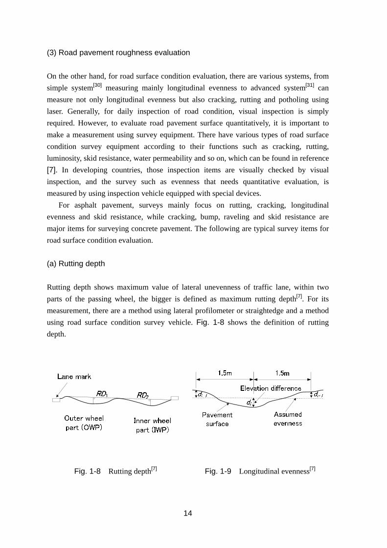
(a) Rutting depth

Rutting depth shows maximum value of lateral unevenness of traffic lane, within two

parts of the passing wheel, the bigger is defined as maximum rutting depth[7]. For its

measurement, there are a method using lateral profilometer or straightedge and a method

using road surface condition survey vehicle. Fig. 1-8 shows the definition of rutting

depth.

Fig. 1-8 Rutting depth[7] Fig. 1-9 Longitudinal evenness[7]

15

(b) Cracking

For the level of cracking, a rate of cracked surface area and the whole area are evaluated.

Cracking rate is usually used for asphalt pavement and cracking degree for concrete

pavement. To measure pavement surface cracking, a method using a sketch and a method

using road surface condition survey vehicle are normally adopted[32].

The rate of asphalt pavement cracking is computed by the following equation. The

cracking area also includes the area of already repaired patching. For concrete pavement,

detail explanation can be found in reference [32].

Cracking rate

100% (1-3)

(c) Longitudinal evenness

Evenness is measured from the level of road longitudinal roughness. For its measurement,

3m profilometer is usually used in Japan and sometimes road surface condition survey

vehicle is also used. As shown in Fig. 1-9, the difference of elevation between pavement

surface and assumed even surface is measured from the points selected more than one

point per 1.5m, and the evenness is expressed by standard deviation of that mean value[32].

Thus, the standard deviation is given by

σ∑

∑

1

(1-4)

where σ is standard deviation ( ), is measurement value of the height ( ), and

is number of measurement value.

(d) International Roughness Index (IRI)

Besides standard deviation described above, the longitudinal evenness is mostly and

globally evaluated by using International Roughness Index (IRI). IRI is an index

introduced by World Bank in 1986, used to evaluate longitudinal evenness of pavement

and riding comfort[33]. As shown in Fig. 1-10, IRI is given by using the motion of virtual

16

uniaxial vehicle model which is called quarter car (QC). In this model, c is damping

factor of vehicle body suspension, k and k are elastic modulus of vehicle body

suspension and tire respectively, m and m are sprung mass and unsprung mass

respectively. When QC runs on road surface with 80km/h speed, IRI is computed by

normalizing the relative velocity accumulation of sprung mass and unsprung mass

divided evaluation distance L. Specifically, IRI is defined as following equation.

IRI| |/

(1-5)

where IRI is International Roughness Index ( / or / ), and are

vertical groundspeed of sprung mass and unsprung mass respectively ( / ), is

running speed, and shows time-domain.

As the larger IRI value is, the shake of vehicle body is also large, thus high IRI

indicates uncomfortable riding. Fig. 1-11 shows the relationship between IRI and road

surface condition. IRI can express road surface condition ranging from 0 to 20, and it is

known that IRI value is about 1 to 4 for paved road surface.

Basically, in order to estimate IRI, there are 4 classes of system responding to their

accuracy[32]. Among those classes, class 3 is widely used to estimate IRI by using the

response of vehicle. For example in Cambodia, World Bank has developed once a year

measurement of IRI using ROMDAS (Road Measurement Data Acquisition System)

modular system for road roughness measurement as shown in Fig. 1-12. Roughness in

IRI measured by ROMDAS was using a bump integrator roughness meter for paved and

unpaved road. And the calibration includes distance calibration, road roughness

calibration and GPS validation. The ROMDAS Proximity Sensor DMI Kit is connected to

the vehicle’s real left wheel. Thus to accurately measure distance, each vehicle needs to

be calibrated against a known 1000m length measured by an electronic distance

measurement device. For roughness calibration, road roughness was measured using dual

ROMDAS bump integrators (see Fig. 1-13). As each vehicle responds differently to

roughness due to variations in the springs, dampers and tires, it is therefore essential to

calibrate each roughness survey vehicle against a standard roughness so that its

measurements can be related back to a standard roughness by regression equations were

calculated for each bump integrator against the 100m wheel path IRI readings for speeds

of 30 and 50 km/h[34]. In this way, we know that there are some difficulties in calibration

and hard to handle with ROMDAS survey, moreover it has to remodel the measured

vehicle to install equipment.

17

Fig. 1-10 Quarter Car model[33] Fig. 1-11 IRI Spectrum[33]

Fig. 1-12 ROMDAS surveyed vehicle

used in Cambodia[20]

Fig. 1-13 ROMDAS Bump Integrator

Roughness Meter[34]

Fig. 1-14 Measuring instruments

for VIMS[35]

Fig. 1-15 Humps calibration

I

18

In the meantime, simplified IRI measurement by VIMS (Vehicle Intelligent

Measurement System) has been proposed by the University of Tokyo[35]. VIMS simply

requires an accelerometer and GPS installed inside the vehicle (see Fig. 1-14) and then

IRI can be obtained by any ordinary vehicles after the vehicle is calibrated. VIMS

estimates IRI through the measurement of acceleration responses of a vehicle driving at

any moderate speed within some range[35]. So it is only need to calibrate the measured

vehicle by using portable humps, as shown in Fig. 1-15, to know its mechanical

characteristics and the transfer function for converting its response to IRI. One more

simple calibration is to get transfer functions corresponding to the driving speed, which

enable the measurement, avoids from the limitation of constant speed driving. For more

details about VIMS, it can be found in reference [35], [36].

However, as the above systems are basically used the response of vehicle to estimate

IRI, so there has some difficulties to measure IRI when the driving speed is extremely

low due to something like traffic congestion. For that reason, in the city of developing

countries which is full of traffic congestion, it is very difficult to estimate IRI by using

these systems.

(4) Road pavement condition evaluation indexes

Again, pavement is one of the important road structures that may easily damage or

deteriorate due to increasing of traffics and loading. So it is necessary to monitor and

evaluate properly the condition of pavement for road network management. Even after

the measurement is conducted, evaluation based on the measurement results is also

important because the repaired action is determined according to the results. In Japan,

some thresholds to decide pavement rehabilitation for asphalt pavement are shown in

Table 1-1. Threshold for other pavements such as concrete pavement, airfield pavement,

and expressway pavement, can be found in reference [37], [38], and [39] respectively.

In addition to these thresholds, and in order to evaluate pavement condition, new

evaluation method using such as fuzzy theory[40] and fractal theory[41] has been considered.

Besides that, several indices have been proposed in the world such as IRI (International

Roughness Index), MCI (Maintenance Control Index), PSI (Present Serviceability Index),

PRI (Pavement Rehabilitation Index), PCI (Pavement Condition Index), PQI (Pavement

Quality Index) etc. Among these indices, in Japan, MCI and PSI are adopted as the

indices expressing the result of road pavement surface survey[35]. MCI is given by

following equation.

MCI 10 1.48 . 0.29 . 0.47 . (1-6)

19

MCI 10 1.51 . 0.3 . (1-7)

MCI 10 2.23 . (1-8)

MCI 10 0.54 . (1-9)

where is cracking rate (%), is mean value of rutting depth ( ), and is

longitudinal evenness ( ). Note that when longitudinal evenness is unknown, MCI is

given by minimum value among the results getting from equation (1-7), (1-8), and (1-9).

In the other hand, PSI is given by

PSI 4.53 0.518 log 0.372 . 0.174 (1-10)

where unit of is . Table 1-2 shows maintenance repair standard by MCI, and

Table 1-3 shows present service ability index and its correspondence repair method.

However, there are some difficulties to express the condition of road pavement using

these indices. From the above equation, as MCI depends much on cracking rate, so it

expresses mainly the quantity of cracking on pavement surface, and it also causes a gap

between MCI value and damage degree at the field. Moreover, it is hard to obtain the data

of cracking rate as well as rutting depth in developing country due to the lack of

measurement equipment. Thus, as described previously, IRI is adopted widely and mostly

in many countries including developed countries, to represent the pavement condition as

well as pavement roughness and riding comfort. From Fig. 1-11, it is known that IRI can

express the condition of road network widely from new paved road to damaged unpaved

road.

(5) Summary on road pavement condition evaluation

As described previously, IRI is simply adopted to evaluate road pavement condition,

and there are many estimation methods have been studied and developed to measure that

IRI value. Recently, the University of Tokyo has developed a very simple system to

measure IRI value, which is called VIMS as described previously. However, this system

still has some difficulties in measuring IRI when the driving speed is extremely low due

to something like traffic congestion. Therefore, in this study, IRI estimation using the

response of motor bicycle which can easily ensure a runway was attempted. And the

development of the simple system for pavement roughness evaluation using such the

response of motor bicycle will be discussed in this thesis and described particularly in

Chapter 4.

20

Table 1-1 Thresholds to decide pavement rehabilitation for asphalt pavement[37]

Road type

Rutting

and

raveling

(mm)

Bump

(mm) Skid

resistance

coefficient

Longitudinal

evenness

(mm)

Cracking

rate

(%)

Potholing

diameter

(cm) Bridge Culvert 8m 3m

Automobile

road 25 20 30 0.25 90 3.5 20 20

High traffic

road 30~40 30 40 0.25 - 4.0~5.0 30~40 20

Low traffic

road 40 30 - - - 30~40 20

Table 1-2 Maintenance repair standard by MCI[42]

MCI Maintenance repair standard

3 or less than 3 Needed repair asap

4 or less than 4 Needed repair

5 and more than 5 Desired control level

Table 1-3 PSI and its correspondence repair method[37]

PSI Repairing method

3 ~ 2.1 Surface treatment

2 ~ 1.1 Overlay

1 ~ 0 Replastering

21

1.3.3 Deterioration prediction of road pavements

It is important to have a proper prediction model of pavement condition for road

maintenance and assessment, but sometimes it is difficult to build the model because

many factors should be considered: road deterioration usually depends on many factors

such as original design, material types, construction quality, traffic volume and axle

loading, road geometry and alignment, pavement age, environmental conditions and

maintenance policy.

Among the several indices to represent road condition, IRI (International Roughness

Index) is generally used to represent the deterioration of pavements, especially in HDM-4

(Highway Development and Management) system that is developed by World Bank.

Road deterioration modelling has developed to predict the future condition and the effects

of maintenance, as well as to support road investment decision. There are many types of

deterioration models such as deterministic models based on statistical analysis of locally

observed deterioration trends and probabilistic model that is good for getting overall

network investment needs. Typical prediction models for IRI such as LTPP (Long-Term

Pavement Performance) model, neural network model and Markov model are explained

in the following.

(1) HDM-4 model

The Highway Development and Management System (HDM-4)[43], originally developed

by the World Bank for international use, is a software tool for conducting pavement

analyses. It is also a decision making tool for checking the Engineering and Economic

viability of the investments in road projects. It can provide not only pavement

performance predictions, but rehabilitation/maintenance programming, funding estimates,

budget allocations, policy impact studies, and a wide range of special application.

The road deterioration models contained in this HDM-4 system attempt to model the

complex interaction between vehicles, the environment, and the pavement structure and

surface. The road deterioration models predict the deterioration of the pavement over time

and under traffic, which is manifested in various kinds of distress. But as each mode of

distress develops and progresses at different rates in different environments, it is

important that the HDM-4 relationships be calibrated to reflect local conditions and to

ensure their relevance to technico-economic analysis of maintenance and rehabilitation

alternatives for a road network constructed in a particular geographical region.

Thus, as the effectiveness of HDM-4 system is dependent on its ability to accurately model and predict pavement performance, which is affected by the accuracy of the input data and calibration efforts[44], so many applications and developments of HDM-4 system in various areas have been studied[45], [11].

22

(2) LTPP model

While HDM-4 model is a model developed by World Bank and has been recommended

extensively to use in developing countries, LTPP model[46] is a model has developed by

the U.S. federal highway administration and can be considered especially with the

pavement in the cold latitudes. In LTPP model, besides pavement structural number and

traffic volume, some other information such as precipitation, number of freeze-thaw

cycles, cooling index and freezing index are also considered for the prediction.

Originally, LTPP model is a part of LTPP program that was envisioned as a

comprehensive program to satisfy a wide range of pavement information needs. LTPP

program draws on technical knowledge of pavements currently available and seeks to

develop models that will better explain how pavements perform. It also seeks to gain

knowledge of the specific effects on pavement performance of various design features,

traffic and environment, materials, construction quality, and maintenance practices. As

sufficient data become available for the program, analyses are conducted to provide better

performance prediction models for use in pavement design and management; better

understanding of the effects of many variables on pavement performance; and new

techniques for pavement design, construction, and rehabilitation. The overall objective of

the LTPP program is to assess long-term performance of pavements under various loading

and environmental conditions over a period of 20 years[47].

The models developed in this program can be used also to predict average rutting or

fatigue cracking trends for a specific regional or statewide environment. Moreover, the

models developed for this program will also be useful in pavement management

applications. As the pavement distress trend models developed in this program can be

used to provide general pavement deterioration trends for a specific environment, these

trends can be used to develop a family of curves for use in a pavement management

system (PMS) where a road highway agency or any local agency does not have sufficient

data to develop those curves[47].

(3) Neural network model

The previous models assume exponential equation as deterioration curve, comparing with

those models there is a model that does not specify the function of deterioration curve but

predicts the deterioration of structures by using neural network. Neural network model is

a nonlinear regression model, and uses data mining in the past for prediction. In pavement

sector, there are many researches applying neural network as an approach in their studies,

such as described following.

Horiki et al.[48] have developed pavement performance forecasting model by using

23

neural network, and then, Shigehara et al.[49] have predicted the progress of pavement

rutting by using neural network model as well. A method for predicting development of

rut depth in asphalt pavements in Hokuriku region of Japan was developed by applying

neural network system. A three layer neural network system with input nodes for

expressway interchange section, subgrade type, lane type, surface type and the number of

large vehicles and an output node for rut depth was employed. The model was established

by inputting performance data of asphalt pavements. The predicted relationship between

rut depth and the number of large vehicles agrees well with observed data.

In similar way, Maekawa et al.[50] have developed a new evaluation method of airport

pavement by using neural network theory. By comparing with the method using multiple

regression analysis, it was found that the method using neural network is effective in

accuracy and output forms, and more accurate comparing with method using the multiple

regression analysis, when it is made more subjectively.

On the other hand, Ozawa et al.[51] have applied neural network to back-calculation of

pavement structure. As structural evaluation of pavement has been conducted by using a

data set of surface deflections measured by a falling weight deflectometer (FWD) and

however, because a back-calculation requires repetitive computation, layer moduli cannot

be estimated instantaneously after FWD tests. Then their study aims to overcome this

shortcoming. Selecting three layer pavements as an example structure, artificial neural

network is trained to acquire knowledge on relationship among layer modulus, layer

thickness and surface deflections. Finally, the system constructed in this manner is

verified by applying the system to FWD test data and by comparing the system generated

layer moduli with those obtained from back-calculation.

(4) Markov model

The above model describes the behavior of pavement deterioration definitely, while a

model using Markov hazard model is also proposed. This Markov model is a stochastic

model which can deal pavement deterioration prediction by stochastic means. In this

model, Markov transition probability is estimated to express the uncertain deterioration

process of pavement, and a choice-based sampling technique is also applied to cope with

the estimation biases caused by sample dropping. Markov model considers the

uncertainty that come between the deterioration process of pavement and uses hazard

model to model the process of deterioration. Note that in this model, it needs large

number of samples to obtain the result with high reliability. Recent researches using

Markov model for structures deterioration prediction will be described in the following.

Tsuda et al.[52] have estimated Markov transition probabilities for bridge deterioration

forecasting. In this study, a methodology to estimate the Markov transition probability

24

model was presented to forecast the deterioration process of bridge components. The

deterioration states of the bridge components were categorized into several ranks, and

their deterioration processes were characterized by hazard models. The Markov transition

probabilities between the deterioration states which were defined for the fixed intervals

between the inspection points in time, were described by the exponential hazard models.

Note that, the applicability of the estimation methodology presented in this study was

investigated by the empirical data set of steel bridges in New York city.

Then, Kumada et al.[53], [54] have expanded the study using this Markov hazard model

to a pavement deterioration forecasting model with reference to sample dropping. In the

study, a pavement deterioration model was presented to forecast the progression of

pavement deterioration based upon the inspection/rehabilitation data. The pavement

performances were described by the multiple rating indices, and the Markov transition

probabilities were modeled by multi-staged exponential hazard model. In the processes, a

part of samples were systematically dropped by preventive rehabilitation activities. So in

the study, a choice-based sampling technique was also applied to cope with estimation

biases caused by sample dropping. Note that, the case study was carried out based upon

the rutting progression data observed on the expressways to illustrate the applicability of

the proposed methodology.

(5) Prediction model for road pavement in developing countries

There are various types of deterioration models from deterministic models to probabilistic

model as mentioned above, and they are selected according to their advantages and the

evaluation purpose. For example, a probabilistic model is good for considering overall

network investment needs, but it cannot be used for planning investments on specific

roads. Additionally, measurement condition affects the selection of model because

sometimes it is difficult to collect the data required in some specific model.

In the case of Cambodia as an example of developing country, according to the

recommendation from World Bank IRI measurement using ROMDAS (Road

Measurement Data Acquisition System) modular system was required to be done once a

year, and also HDM-4 system is required for road asset management including

maintenance planning, budgeting and operations[8]. To complete the management using

this system, it requires a lot of information, such as IRI, FWD deflection, traffic, area of

cracking, rutting depth, number of potholes and so on. However, in Cambodia only IRI,

FWD deflection and traffic information are available even though they adopt HDM-4

system. Thus, the performance of prediction models with such limited information should

be clarified.

25

1.4 A simple management system for road pavements in developing countries

In developing country, there are many issues caused by insufficient engineers,

technologies development, and especially maintenance budget, for road pavement

management. Furthermore, most of pavements in developing countries are DBST

pavements. Besides the structure itself, the deterioration condition including the

surrounding environment such as traffic load, weather in developing countries are

peculiar. Therefore, the existing methods described in section 1.3 may not be adequate

for pavement management in developing countries and simple method with acceptable

accuracy and low cost using a simple device is inevitably required to ensure pavement

performance in developing countries.

To build the simple system to evaluate the pavement condition, first proper prediction

model should be constructed. Secondly simple evaluation system for pavement condition

should be developed. In the evaluation system, surficial condition such as roughness

should be focused on because roughness can be represented by IRI which is widely

adopted and directly related to riding comfort. The structural condition such as stiffness

of layers in pavement is also important factor to be considered. In addition to them, traffic

information such as actual live load is important either. Thus in the simple system, these

factors should be at least evaluated. The relationship and significance of each component

in management system is conceptually illustrated in Fig. 1-17.

For simple pavement deterioration prediction, as described in section 1.3.3, as most

of needed data used for the deterioration prediction in developing country seem

insufficient, the performance of prediction models even with such limited information

should be clarified. And a simple prediction model using fundamental data of such as IRI

values which represent pavement surface condition, FWD and traffic loads should be

developed. Thus herein the prediction behavior of representative existing models will be

examined and compared in Chapter 2, to obtain the proper model under limited

information.

As described in section 1.3.2 (1), since FWD test requires large-scale measurement

devices and much cost, a simple structural evaluation method using impact load and

impact sound will be developed and verified in Chapter 3. Moreover, as described in

section 1.3.2 (2), simple IRI estimation using the response of a motor bicycle which is

most available and cheap transportation in developing countries will be developed and

verified in Chapter 4.

In general it is difficult to grasp the real traffic loads of each road in different region.

In developing country, traffic loads are basically surveyed by weigh in motion station[20].

But because it requires a specific equipment and too high cost to manage the facilities,

and additionally, repairing cost is also high when it is in failure, a stable observation

26

cannot be attained. Thus, in this study Bridge Weigh-In-Motion (B-WIM) system will be

applied to live load monitoring in Thailand as described in Chapter 5.

Fig. 1-16 shows one example of management sequence using simple methods. Using

the proper prediction model, the total cost of maintenance could be calculated. Then the

optimum strategy of maintenance to minimize the total cost based on the deterioration

prediction and current evaluation of pavement condition can be established.

Fig. 1-16 Overview of PMS flow[37]

Current condition of

pavement

Database

Deterioration prediction

Maintenance and repair

Pavement condition

evaluation

Reflection

27

Fig. 1-17 The procedure of suggested PMS

Current evaluation of pavement condition

Maintenance and repair strategy

Simple deterioration

prediction

Databank

Simple surface

evaluation

Simple structural

evaluation

Simple

traffic load

IRI measurement

by vehicle or

motor bicycle

Impacting load and

Impacting sound

B-WIM

system

Visual inspection

Acceptable

value?

Exponential model or

Markov model

Acceptable

value?

Yes Yes

No No

28

1.5 Objective and scopes

The purpose of this study is to develop a very simple method of structural evaluation,

roughness evaluation, and as well as live load evaluation for road pavement management

in developing country that face extremely on limitation of budget allocated for the

maintenance/repair/renewal of infrastructures. This study also examines the behavior of

IRI prediction models in order to find out the most simple, available and adequate for

pavement condition evaluation.

This study consists of 3 steps: in the first step, the author examines the behavior of

IRI prediction models in order to find out the most simple, available and adequate for

pavement condition evaluation. Then, the simple methods of structural pavement

evaluation and pavement roughness evaluation are developed in the second step. Finally,

in the third step, the effect of applying load on pavement fatigue is evaluated when actual

live load is considered instead of design load on the basis of current traffic data by Bridge

Weigh-In-Motion system.

In Chapter 2, IRI prediction models with only the information of IRI, FWD deflection

and traffic volume are examined. Herein the author adopts five models of HDM-4, LTPP,

neural network model, Markov model and exponential model which is built by the

authors with consideration of data trend. First, we study the influent factors of IRI

increment by using detail survey data from Cambodian national road No.5. After using

survey data from all Cambodian national roads to build each model, the actual data of

Cambodian national roads No.5 are used to examine the prediction behavior of those

models. Here, by using survey IRI in year 2010 to predict IRI in year 2011 then the author

compares the prediction results to the actual data obtained in year 2011.

For developing a simple method of structural pavement evaluation, Chapter 3

describes the application of impacting technique including impacting load and impacting

sound to structural soundness evaluation of road pavement, by using pavement with thin

layers as target pavement. Herein, first after impacting the surface of four model

pavements that have different physical properties (layer thickness and stiffness) by impact

hammer, impacting load and impacting sound were recorded and evaluated. Then, the

correlations between impacting feature values and physical properties of each pavement

layer were confirmed. Next, numerical model of model pavement using FEM dynamic

analysis was built to represent the impacting test. And then parametric analysis of the

numerical model was studied to confirm the applicability of impacting method.

For developing a simple method of pavement roughness evaluation, Chapter 4

describes the development of IRI estimation using the response of motor bicycle that can

easily ensure a runway in the cities within traffic congestion. And as motor bicycle is a

major transportation in most of developing countries, it can be said the measurement

29

system using motor bicycle is more simple system than that using vehicle. Herein, the

system estimated IRI using motor bicycle is proposed and also, validity of the system is

verified from the field tests. Note that the proposed system is basically applied by the

measurement principle of VIMS[35], the system that estimates IRI using sprung mass

response of vehicle.

For a simple method of applied live load evaluation, Chapter 5 describes the effect of

applying load on pavement fatigue when actual live load is considered instead of design

load on the basis of current traffic data by using Bridge Weigh-In-Motion system in

Bangkok city, Thailand.

Chapter 6 reviews the several conclusions that can be drawn from this study.

30

31

Chapter 2 Evaluation of IRI prediction models

with limited information

2.1 General remarks

Recently, in Asian countries such as Cambodia, road pavement tends to deteriorate faster

than expected, which may stop traffic and disturb the economic progressing. Thus it is

important to have a proper prediction model of pavement condition for road maintenance

and assessment.

In general, IRI (International Roughness Index) is used for management of road

network, especially with HDM-4 (Highway Development and Management) system that

is developed by World Bank. To complete the management using this system, we need a

lot of information, such as IRI, FWD (Falling Weight Deflectometer) deflection, traffic,

area of cracking, rutting depth, number of potholes and so on. However, in Cambodia

only IRI, FWD deflection and traffic information is available even though they adopt

HDM-4 system. Thus the performance of prediction models even with such a limited

information should be clarified.

Beside HDM-4 model, there are some models have been developed to predict IRI

such as LTPP (Long-Term Pavement Performance) model, neural network model and

Markov model. LTPP model is a model developed by the U.S. federal highway

administration and can be considered especially with the pavement in the cold latitudes

when neural network model is a prediction model using data mining and Markov model is

a stochastic model. In many developing countries as well as Cambodia, most of needed

data used for the prediction of pavement deterioration seem insufficient, so it is very

meaningful to make clear about prediction behavior of those models in such that

condition.

In the study of this chapter, the author evaluates IRI prediction models with only the

information of IRI, FWD deflection and traffic volume. Herein the author adopts five

models of HDM-4, LTPP, neural network model, Markov model and exponential model

which is built by the authors with consideration of data trend. First, the author studies the

influent factors of IRI increment by using detail survey data from national road No.5.

After using survey data from all national roads to build each model, the actual data of

national roads No.5 are used to examine the prediction behavior of those models. Here,

by using survey IRI in year 2010 to predict IRI in year 2011 then the author has compared

that prediction results to the survey IRI in year 2011.

32

2.2 General outline of this chapter

2.2.1 Survey data

In Cambodia, the pavement of national road managed by MPWT (Ministry of Public

Works and Transport) has total length about 2100km and can be divided mainly in two

types, AC (Asphalt Concrete) pavement and DBST (Double Bituminous Surface

Treatment) pavement. In all types of pavement, more than 60% is DBST pavement

because it is a kind of low cost pavement.

Table 2-1 shows the year of data that is recently surveyed by MPWT and used for

this study. In the listed year, IRI value, FWD deflections, traffic volume, structural

numbers and CBR value are surveyed. In IRI measurement, IRI definition uses 100m

intervals, FWD deflections are measured at 200m intervals, and structural numbers and

CBR are measured at 2km intervals. The traffic information is obtained at several

locations of each road. The measurement system used for FWD deflection is KUAB

Falling Weigh Deflectometer with Dynaflect. And the measurement system used for IRI is

mainly ROMDAS system, but VIMS system is used only in 2011.

National road No.5 that is used to examine the models is located from Phnom Penh

the capital of Cambodia to Thai border and the total length is about 405 km. Table 2-2

shows the data of road No.5 including the type of pavement, the completion year of

rehabilitation, IRI and the statistic data of IRI of each section. After rehabilitation, the

pavement of the section from 0 to 356 km is replaced by DBST (Double Bituminous

Surface Treatment), and that of the section between 356 ~ 405 km is replaced by AC

(Asphalt Concrete) pavement. The thickness of each layer of DBST pavement measured

from national road No.5 is shown in Table 2-3.

2.2.2 Transition of IRI

Fig. 2-1 shows the transition of IRI obtained in national road No.5. Here, Note that the

data herein is obtained in 2004 and 2011. From this figure, it is clearly observed that IRI

of the section between 0 ~ 91km and 356 ~ 405km decrease significantly. This may

correlate the fact that the pavement around big cities has been rehabilitated. When IRI of

the year 2005 from section between 171 and 301km and that of the year 2010 from

section between 356 and 405km, IRI of AC pavement seems smaller than that of DBST

pavement in the same service period.

33

Table 2-1 Survey year of data set of each national road

National

road

Distance

[km] IRI FWD

Traffic

volume

Structural

numbers CBR

No.1 About

166

2004

2005

2010

2009 2010 - -

No.2 About

120

2004

2005

2010

2009 2010 - -

No.3 About

201

2004

2005

2010

2009 2010 - -

No.4 About

214

2004

2010 2009 2010 - -

No.5 About

405

2004

2005

2010

2011

2009 2010 2011 2011

No.6 About

415

2004

2005

2010

2009 2010 - -

No.7 About

450

2004

2010 2009 2010 - -

34

Table 2-2 Basic data of national road No.5

Distance Pavement

Type

Completion Year

of

Rehabilitation

Measured IRI [m/km]

Date Average Standard

Deviation

0 ~ 91km DBST Mid 2004 Jan. 2004

July 2011

4.96

3.82

1.58

1.49

91 ~ 171km DBST May 2004

Jan. 2004

March 2005

2010

July 2011

5.34

3.54

3.76

3.50

3.15

1.05

0.91

0.88

171 ~

301km DBST Dec. 2003

Jan. 2004

March 2005

2010

July 2011

3.33

3.00

2.85

3.38

0.74

0.67

0.60

0.99

301 ~

356km DBST April 2004

Jan. 2004

March 2005

2010

July 2011

3.83

3.24

3.34

2.97

1.38

1.04

0.81

0.85

356 ~

405km AC 2008

Jan. 2004

2010

July 2011

5.17

1.48

1.81

2.59

0.54

0.47

Table 2-3 The thickness of each layer of DBST pavement from national road No.5

Each layer Minimum value Maximum value Average

Surface layer [mm] 0 60 24.7

Base course [mm] 0 360 155.7

Sub-base [mm] 0 1320 296.0

Sub-grade CBR [%] 3.5 50 23.3

35

Fig. 2-1 IRI History

2.2.3 Relationship between IRI increment and influential factors

To find out the relationship between IRI increment and influential factors, the IRI data in

the section from 95 to 171km and that from 294 to 356km at the period from year 2010

and 2011 are used because in these years and sections information about structural

number is known and also no any repair work during that period is confirmed.

Because traffic volume is an important factor which may affect the pavement

roughness, the traffic volume of heavy vehicles was divided into two categories: low

traffic and high traffic. Note that because the traffic volume of almost all the sections in

No.5 correspond to N5 category the traffic volume is divided by comparing with the

volume to the average number of large vehicles.

Fig. 2-2, Fig. 2-3 shows the relationship between IRI increment and IRI, FWD

deflection respectively. Note that FWD deflection was obtained by DMD (Dynaflect

maximum deflection). From these figures, it is difficult to recognize any linear relation

between FWD deflection and IRI increment, but the linear correlation between IRI and

IRI increment has been confirmed. It is also found that the correlation is stronger in low

traffic than that in high traffic. Moreover, no significant linear relation between other

factors can be found.

Therefore, IRI increment has almost no linear correlation with FWD deflection as

well as other factors but has high correlation with IRI itself and that correlation becomes

strong for low traffic.

36

Fig. 2-2 IRI (year 2010) and IRI Increment

Fig. 2-3 FWD deflection and IRI Increment

0 2 4 6 80

1

2

3

4

IRI [m/km]

dIR

I [m

/km

]

Low Traffic (Correlation coefficient = 0.73)High Traffic (Correlation coefficient = 0.53)

0 0.2 0.4 0.6 0.8 1 1.20

1

2

3

4

FWD Deflection [mm]

dIR

I [m

/km

]

Low Traffic (Correlation coefficient = -0.11)High Traffic (Correlation coefficient = -0.09)

37

2.3 IRI prediction models

In this study five kids of prediction models are used: HDM-4 model that is actually

applying in Cambodia, LTPP model as a prediction model in developed country,

exponential model consist of only basic parameters, neural network model using data

mining and Markov model as stochastic model. Note that FWD deflection using here is

the value measured in 2009, and during the period for prediction, this value is assumed to

be constant. In addition, because the output is different in stochastic model such as

Markov model and the other deterministic models, the error of prediction and also

probability of the state of pavement are compared after each model yields the result.

2.3.1 HDM-4 and LTPP model

HDM-4 model is originally developed by World Bank and has been recommended to use

in developing countries. LTPP model is developed by the U.S. federal highway

administration and basically used only in the U.S. In these models, IRI can be predicted

by using the year to be known and the original state of IRI are used as an input parameter

for prediction. Herein, IRI data of year 2010 is used to predict IRI in year 2011 and then,

and the result is verified with actual IRI data measured in year 2011. In HDM-4 model,

incremental change in roughness due to structural deterioration, cracking, rutting,

potholing and the environment should be considered and sum up for IRI prediction. On

the other hand, in LTPP model, besides structural number and traffic, precipitation,

number of freeze-thaw cycles, cooling index and freezing index are also considered for

the prediction. Because of lack of the information about cracking, rutting and potholing,

the effect of these factors is excluded in this study.

Fig. 2-4 shows the relationship between the measured IRI and IRI predicted by

HDM-4 and LTPP model. From the figure, it is observed that the error becomes larger

over 5 of IRI value in HDM-4 model. This may be caused by the fact that the information

on the cracking, rutting and potholing effect is neglected. In LTPP model, all predicted

IRI are smaller than measured IRI and that the gap becomes large when IRI is over 5.

Probably because LTPP model is used especially for AC pavement and the model may

recognize DBST as worst condition and give underestimated values. Thus it can be said

that these models are used for the prediction of IRI in national road No.5, but the model

underestimate IRI as IRI increases.

38

Fig. 2-4 IRI prediction using HDM-4 and LTPP model

2.3.2 Exponential equation model

In HDM-4 and LTPP models, the relationship between IRI increment and influential

factors are expressed by exponential function because the statistical data from the past

investigation in United States and the other counties shows such relationship. Since the

information like cracking, rutting and potholing needed in HDM-4 are hard to acquire in

Cambodia, they neglect these factors. Although there is no linear relationship between

FWD deflection and IRI increment as shown in the previous description, the error rate of

IRI prediction had improved about 10% when we considered FWD deflection and traffic

as parameters. Thus, herein the author built an exponential model with consideration of

these factors expressed as

Δ Δ (2-1)

where Δ : IRI increment from year to year , : IRI from year , Δ

: a period for IRI prediction (year), : FWD from year and are

coefficients. Unknown parameters in equation (1) were determined by applying nonlinear

least-squares method to the actual data from year 2004 to year 2010. Note that the

equation does not have a parameter with regard to traffic, but the author determines the

coefficients according to low and high traffic respectively. The results from fitting data

are shown in Table 2-4.

0 2 4 6 80

2

4

6

8

Measured IRI [m/km]

Pred

icte

d IR

I [m

/km

]

HDM-4LTPP

39

Next, to verify the model, IRI of national road No.5 in 2011 is predicted by the model

using the IRI in 2010 and is evaluated by the actual measured data. The result of

prediction shows in Fig. 2-5. From the figure, it can see predicted IRI and measured IRI

have a pretty agreement between each other and also the error rise as IRI increases, which

is also confirmed in HDM-4 and LTPP model.

Table 2-4 Coefficients from fitting data

Coefficients Low Traffic High Traffic

0.6283 0.2693

-1.1919 1.1110

0.3344 -9.1743

0.2155 -0.2115

-0.1023 0.0018

Fig. 2-5 IRI prediction using exponential model

0 2 4 6 80

2

4

6

8

Measured IRI [m/km]

Pre

dict

ed I

RI

[m/k

m]

Low TrafficHigh Traffic

40

2.3.3 Neural network model

The previous models assume exponential equation as deterioration curve. However there

is a model that does not specify the function of deterioration curve but predicts the

deterioration of structures by neural network. Horiki et al.[48], Shigehara et al.[49] have

predicted the progress of pavement rutting by using neural network model that is

nonlinear regression model. In this study, neural network model is applied for IRI

prediction by assuming the roughness deterioration progress as time-series pattern. In the

meantime, traffic volume, FWD deflection and IRI surveyed value have been assumed as

influence factors and are used for input parameters. Then, the hierarchical type of neural

network was used and error back propagation method was adopted as learning process.

For detailed explanation such as calculation formula, it can be found in the reference [48]

and [49]. Note that neural network model is used for short term prediction, and one year

increment of neural network model was built.

The assumed neural network model has 3 layers including 3 nodes of input layer, 20

nodes of inner layer and one node of output layer. The input-output nodes and their

parameters are shown in Table 2-5. As it is known that the performance of neural

network model is improved due to normalizing input value, traffic volume is assigned to

0 and 1 corresponding with low and high traffic respectively. Similarly with FWD

deflection, deflection smaller than averaged value is considered as low bending capacity

pavement, deflection bigger than averaged value is considered as high bending capacity

pavement and they are assigned to 0 and 1 respectively. Also, IRI measurement values

and IRI increments are normalized as between 0 and 1.

For deterioration prediction, the data of all national roads from year 2004 to 2005 are

used as training data to predict IRI value after one year from year 2010 of national road

No.5. First, in order to confirm the influence of each parameter, IRI increment is

confirmed when traffic volume and FWD deflection were fixed with the model after

training. The results are shown in Fig. 2-6. In the figure, the actual values are also plotted.

Note that the actual values are averaged with the range integer value of IRI. From the

figure, it is observed that in case of low traffic, IRI increment tends to be small when IRI

value is small. However, in case of high traffic, IRI increment increases much from the

stage of small IRI value. That means IRI value increases slowly for small IRI value, and

increases rapidly for large IRI value in the case of low traffic. Also in case of high traffic,

IRI value increases rapidly even for small IRI value. These trends are reasonable when

the interaction of pavement and live load is considered.

Next, the contribution ratio of each parameter is calculated using weighting factor

obtained in the process of training. Herein, the contribution ratio, , according to

input node is given by

41

∑

∑ ∑ (2-2)

where is weighting factor from node to node. N and N is total number node

of input layer and inner layer respectively. The calculation result is shown in Table 2-6.

From the table, it is observed that even the influence of IRI value is high which is also

confirmed in the other models, the contribution ratio of each parameter is almost identical,

about 30% each, and thus it can be said that each parameter equivalently affects the

output results in NN model.

Finally, the relationship between actual IRI value in year 2011 and the IRI value

predicted by neural network model based on the IRI measured value in year 2010 is

shown in Fig. 2-7. In this figure, to match with the other prediction models, the

prediction value is divided to low traffic and high traffic. From the figure, it is observed

that for IRI value less than about 5m/km, the predicted IRI is agree with that measured

for all traffic volumes. Also as it confirmed in the other models, it tends to underestimate

IRI when its value is over than 5m/km, and it can be said that even NN models cannot

improve this underestimate.

Table 2-5 Data to be used in neural network model

Node Option Choices

Input

Traffic volume Low 0

High 1

FWD deflection Large 0

Small 1

IRI Measurement value 0 ~ 1

Output IRI increment Increment size 0 ~ 1

Table 2-6 Contribution ratio of each factor

Each factor IRI Traffic

volume

FWD

deflection

Contribution ratio 37% 31% 32%

42

Fig. 2-6 Progression of IRI deterioration using neural network model

Fig. 2-7 IRI prediction using neural network model

1 2 3 4 5 6 7 80

0.2

0.4

0.6

0.8

1

1.2

1.4

1.6

1.8

2

IRI [m/km]

IRI In

cre

ment

[m/km

]

High Traffic＆Large FWDHigh Traffic＆Small FWDLow Traffic＆Large FWDLow Traffic＆Small FWD

0 2 4 6 80

2

4

6

8

Measured IRI [m/km]

Pre

dic

ted IR

I [m

/km

]

Low TrafficHigh Traffic

43

2.3.4 Markov model

The above models describe the behavior of pavement roughness deterioration

deterministically, while Tsuta et al.[52], Kumada et al.[53], [54] predict the deterioration by

using Markov hazard model which is stochastic model. They estimate Markov transition

probability that expresses the uncertain deterioration process of pavement and a

choice-based sampling technique is also applied to cope with the estimation biases caused

by sample dropping. In Markov model, the uncertainty in the deterioration process of

pavement is considered and hazard model is built to model the process of deterioration.

Note that in this model, large number of samples is needed to obtain the result with high

reliability. In this study continuous IRI measured value is transformed into discrete values

and Markov transition probability is estimated by using exponential hazard model. For

detailed explanation such as formulation and the way of estimation, it can be found in the

reference [52], [53] and [54].

Because the values of IRI in No.5 are almost in the range between 2 to 5m/km and the

classification for the value less than 1m/km is not reasonable, IRI value is rated in

5-grades as shown in Table 2-7. In this model, the parameters of FWD deflection and

traffic volume are explanatory variable. IRI itself is not explicit input in this model but

different models corresponding to IRI ratings are built. FWD deflection and traffic

volume are normalized by dividing the data by the maximum value. The data of all

national roads is used for analysis, but the data of section that damage degree is improved

due to rehabilitation, is excluded. Note that it is known that this kind of exclusion yields

some estimation bias caused by sample dropping such as excluded data is applied with the

estimation biases caused by sample dropping, but in this time of study, it is not

considered.

Table 2-8 shows the parameters estimated by multistage exponential hazard model.

Note that damage level 5 is final state and thus the state of 5 always keeps this position

after it is reached. In the same table, likelihood ratio to indicate the estimation accuracy of

the model, and t value are listed. Note also that when the likelihood ratio is over than

14.86, null hypothesis can be discarded due to no interpretability on the model for 99.5%

level of significance. From the table, it is observed that the likelihood ratio is 1496 which

indicates the sufficient interpretability on the model. In the meantime, when t value is

over than 1.96, null hypothesis can be discarded due to no interpretability in the model for

95% level of significance. Note that in the table, “-” indicates the case where t value is

less than 1.96. Note also that the constant term is explicitly shown in the case of damage

level 4, even though the t value is less than 1.96. This is because the constant term is

needed to calculate likelihood ratio but it has 80% level of significance for interpretability

in this case.

44

From the table, as for FWD, it is observed that it has interpretability in damage level 1

but has no interpretability in damage level more than two. And it can be said that traffic

volume has much influence on the probability in the state damage change from level 4 to

5. This fact means that FWD has influence on the probability when deterioration is small

but when the deterioration becomes significant, traffic volume has influence on the

probability. t values of FWD in damage level 3 as well as the constant term in damage

level 4 are small partly because of small number of samples. Thus to evaluate the

deterioration properly by this model, it is necessary to accumulate a lot of reliable datum.

From the estimation result, expected hazard rates, , rating life expectancies,

, are calculated and their results were shown also in Table 2-8. From the life

expectancy, it can be observed that minimum expectancy is 4 for low level damage but

maximum year is 8 for high level damage. The reason that life expectancy is such long

for high level damage, because the number of sample is not sufficient in high level

damage and thus the occurrence probability necessarily decreases due to the lack of

samples. Fig. 2-8 and Fig. 2-9 show the expected value pass of damage level according

to traffic volume and FWD deflection, respectively. In this figure, “mean” indicates the

mean values and “maximum” and “minimum” also indicate the maximum and minimum

values, respectively. From the figure, according to the expected value pass, it is observed

that the influence of traffic volume is higher than that of FWD deflection. Next, in order

to examine the prediction performance of this model, Markov transition probability

matrix is obtained by two ways such as averaging operation and enumeration. Herein,

averaging operation is the method to obtain the transition probability matrix by using the

expected values of hazard rate shown in Table 2-8 to average the influence of factors..

Note that in averaging operation the datum from year 2004 to year 2005 are used.

Enumeration is the method to obtain the matrix by enumerating the transition percentage

of each value. Note also that the date in year 2004 and year 2005 is used in enumerating

method. Markov transition probability matrixes obtained by two methods are shown in

Table 2-9 and Table 2-10. Then, to predict the damage state probability of year 2011,

each matrix is multiplied by damage state probability of year 2010. Finally, the

relationship between actual measured value and predicted value of damage state

probability of year 2011 is obtained as shown in Fig. 2-10. From the figure, it is clarified

that the measured values and predicted values agree with each other, which may indicate

that this model is valid.

45

Table 2-7 Rating of IRI

Damage degree Measured IRI [m/km]

1 Less than 2

2 2 ~ 3

3 3 ~ 4

4 4 ~ 5

5 5 and over

Table 2-8 Results from the estimation

Damage

degree Constant FWD

Traffic

volume

(years)

1

(t value)

0.1227

(4.73)

0.2444

(5.32)

0.1303

(5.39) 0.2856 3.5016

2

(t value)

0.1342

(5.14) -

0.1929

(5.14) 0.2143 4.6673

3

(t value)

0.0513

(3.38) -

0.1219

(5.49) 0.1202 8.3163

4

(t value)

0.0604

(1.53) -

0.1066

(2.10) 0.1142 8.7569

Initial likelihood (model of only constant term) : 6323

Final likelihood (model including all parameters) : 7071

Likelihood ratio : 1496

46

Table 2-9 Estimation result (Transition probability matrix)

Damage degree 1 2 3 4 5

1 0.7516 0.2225 0.0249 0.0010 0.0000

2 0 0.8071 0.1813 0.0111 0.0004

3 0 0 0.8867 0.1069 0.0064

4 0 0 0 0.8921 0.1079

5 0 0 0 0 1

Table 2-10 Transition probability matrix by Numeration

Damage degree 1 2 3 4 5

1 0.6308 0.3201 0.0397 0.0070 0.0023

2 0 0.5561 0.3494 0.0819 0.0127

3 0 0 0.7569 0.2039 0.0392

4 0 0 0 0.7486 0.2514

5 0 0 0 0 1

47

Fig. 2-8 Deterioration expected value pass (the change of traffic volume)

Fig. 2-9 Deterioration expected value pass (the change of FWD deflection)

Fig. 2-10 State probability of IRI prediction using Markov model

0 10 20 30 40 505

4

3

2

1

Duration [years]

Dam

age leve

l

meanminmax

0 10 20 30 40 505

4

3

2

1

Duration [years]

Dam

age leve

l

meanminmax

0 20 40 60 80 1000

20

40

60

80

100

State probability of measured IRI [%]Sta

te p

robab

ility

of

pre

dicte

d IR

I [%

]

NumerationEstimation

48

2.3.5 Comparison of prediction models

Finally, mean square errors between the actual value and estimated values of all models

are shown in Table 2-11. Note that the results of Markov model cannot be considered

herein because this model yields only state probability. From this table, it is confirmed

that the error of neural network model and exponential equation model is small, but that

of HDM-4 and LTPP is large.

Next, in order to compare the performance of Markov model with other models, the

continuous IRI values predicted from determined model are rated following by Table 2-7,

and then the state probability of that predicted values is calculated. In addition to this state

probability, the number of each state data is defined so the relative errors of each damage

state are calculated and averaged. Therefore, according to the damage state, when the

number of actual measured value is , and the number of predicted value is , so the

average of relative errors, , can be defined as following equation.

1∑

(2-3)

The result of averaged relative errors from each model is also shown in Table 2-11.

From this table, it is known the result of enumeration has relative error smaller than that

of Markov model. Moreover, it is found exponential model express less error comparing

with all other models.

Table 2-11 Comparison of each model

Models Mean square error Relative error

HDM-4 0.5677 0.0402

LTPP 0.8683 0.0803

Exponential 0.2057 0.0201

Neural network 0.2919 0.0434

Markov - 0.0811

Numeration - 0.0530

49

2.4 Summary

In this chapter, as in most developing countries such as Cambodia, the information used

for the pavement deterioration prediction seems insufficient and hard to acquire. Then in

this study, a very simple prediction model for Cambodian national road pavement

roughness is developed by using only the data of IRI, FWD and heavy vehicle traffic.

Herein five prediction models of HDM-4, LTPP, exponential equation, neural network

and Markov model are considered and discussed. The actual data of all 1-Digit

Cambodian national roads are used to build the models, and the actual data in year 2011

of national roads No.5 are used to examine the models. Besides the prediction, the

influence of several factors on the rate of IRI increment was also evaluated. The main

results from the study are resumed as following.

(1) By evaluating the influence of several factors on the rate of IRI increment, it was

found that IRI increment strongly depends on IRI value itself but the other factors

such as FWD deflection, structural number, are not significant.

(2) For the prediction by HDM-4 model, the necessary factors such as cracking,

rutting and potholing are not considered herein. This neglect may lead to smaller

values than the actual measured values when the IRI is high. Also in LTPP model,

almost all the values of IRI are underestimated.

(3) In the exponential model determined by actual surveyed data, it is found that the

prediction result agrees well with the actual values. Neural network model also

shows good agreement with the actual values but the error becomes large when

the IRI value is over 5m/km.

(4) In Markov model by averaging operation, even though several influence factors

can be considered, the error is larger than that by enumeration method due to the

lack of the number of data.

(5) Finally it is clarified that FWD deflection and traffic information are significant

in the IRI prediction, and that the result predicted by exponential model can yield

the smallest error than that of the other models

Therefore, for Cambodian national roads No.5 where the data is limited, IRI value can

be predicted well by using exponential equation model. Moreover, because the

exponential model is built by using all the data of 1-Digit national roads, it is possible to

apply this prediction model to the other national roads. On the other hand, the other

models that have not enough input parameters can be possibly used also for IRI prediction,

however the error becomes large when the value of IRI is large. Note that in the future

when road pavement is properly maintained and the necessary input data is given with

50

high reliability, the other models might be express higher prediction performance. So it is

very important to collect the data regularly at the field site.

Note that this exponential function model requires only IRI value, traffic information

and FWD deflections to predict pavement deterioration. But as it is difficult to measure

FWD deflections, so FWD deflections should be replaced by impedance ratio of

impacting load and dominant frequencies of impacting sound which can represent also the

stiffness of the pavement (see Chapter 3). However, when enough of measurement data is

available, and it is for network level, Markov model should be better applied for the

prediction. Thus, herein the author suggests a simple prediction model for pavement

deterioration that should be decided by the data condition and analysis level as shown in

Fig. 2-11.

Fig. 2-11 Prediction model decision flow

IRI measurement Impacting test Traffic load

Visual inspection

Sufficient data?

Network level?

Exponential

model

Exponential

model Markov model

No

No

Yes

Yes

51

Chapter 3 Development of an evaluation

system of pavement structures

based on impact testing

3.1 General remarks

Recently, in developing countries such as Cambodia, highway road paved by asphalt

tends to deteriorate faster than expected, not only due to the quality control during

construction but the proper maintenance after in service[8]. Generally, to evaluate asphalt

pavement after in service, functional deterioration such as cracking, deformation, raveling,

and structural deterioration such as low bearing capacity of each layer have to be

considered[7]. In developing countries, associated with a road management system

recommended from supporting countries, evaluation systems for road surface condition

and structural pavement have been introduced[8].

At the present, for structural pavement evaluation systems, surface wave method[18],

as well as FWD (Falling Weight Deflectometer) test[19] have been mainly used. FWD test

is a method used by applying impacting load to road surface and the occurred deflection

is measured to evaluate structural conditions of pavement[55]. From the waveform of

deflection data, it is also possible to estimate characteristic values of each pavement

layer[22].

In practice, FWD test is widely used in many countries in the world including

developing and also developed countries. However, for FWD test, traffic control and lots

of times is inevitably required to measure the road in long distance. For that reason,

recently various devices have been proposed to measure the surface deflection

continuously at high speed in order to make time savings of measurement[23]. Surely these

devices can reduce the time and labor drastically, but they need extraordinary cost to do

measurement, and thus they are still unavailable for developing countries that have no

enough budgets for maintenance system.

On the other hand, it is well known that the impact sound caused by impacting an

object includes contact sound between the objectives, and pneumatic pressure vibration

sound occurred from vibration of the object surface[24]. Thus, the impacting sound can be

used for evaluation of the object. Generally the objective can be evaluated roughly by

52

hearing the impact sound but also more precisely by analyzing the sound in detail to

obtain the objective's physical properties. Previously researches on structural evaluation

by analyzing the impact sound have been done widely in the field of concrete

structures[25]. It has been clarified that internal defect or surficial deterioration can be

detected by the impact sound[26]. Felicetti[27] assessed an industrial pavement via the

impact acoustics method to clarify the possibility of physical property evaluation of

structures as asphalt pavement using impacting sound.

Not only the impact sound but also impacting load or repulsive load itself reflects to

surface hardness and stiffness of structures, and then by analyzing impacting load it is

possible to evaluate the physical properties of the target structures. To investigate the

surficial quality of concrete structures, test hammer method[28] and impedance method is

currently used. In test hummer method, when the structure is impacted by a specific

hummer, rebounding height of a hummer head is measured. Impedance method[29] uses

the mechanical impedance ratio of impacting load which is a ratio of acting and reacting

forces obtained in the waveform of loading.

In developing countries, mostly DBST (Double Bituminous Surface Treatment)

pavement is adopted because of its low cost, and thus it may be possible to investigate the

surficial quality by analyzing the impact load and sound, because DBST is relatively thin

and even small load of impact hummer can be applied to deform the structure of DBST.

Thus when the impact method is applied to the evaluation of pavement, it may reduce the

cost for investigation although it still requires time to execute comparing with FWD

method.

In this chapter, to develop a very simple method for structural evaluation of road

pavement in developing countries where thin layers are widely used such as DBST,

impact method using impact load and sound are applied for structural evaluation. Herein,

first experimental study was conducted using a model pavement where four types of

layers having different physical properties (layer thickness and stiffness) are constructed.

In this experiment, impact load and sound are investigated to evaluate the surficial

stiffness of pavement, and the correlations between impacting features such as dominant

frequencies of impact sound and mechanical impedance of impact load, and physical

properties of each pavement layer were confirmed. Next, parametric study was conducted

using numerical models to clarify the factors determining the impacting features. In this

analysis, several thickness and stiffness of layers were considered and dynamic

simulation was conducted using FEM analysis to obtain the surficial waveform of

pavement which can be regarded as a source of impact sound.

53

3.2 Impact test on model pavements

3.2.1 Model pavements

To model the simple asphalt pavement in developing countries, four different model

pavements having different layers are constructed as shown in Table 3-1. A-section is a

standard pavement, B-section is a pavement having thick base course, C-section is a

pavement having thick surface layer and D-section is a pavement with low bearing

sub-grade. These pavement sections are constructed side by side with 2m distance apart

from each other and have 2m times 2m effective length and width. Table 3-2 shows the

material used in each layer of model pavement and the actual properties obtained in the

site test are shown in Table 3-3.

To estimate the physical properties of the model pavements, the model pavements

were impacted by the instrumented hummer that can record the impact force, and the

impact sound is recorded by sound level meter. In addition to them, portable FWD was

applied to obtain the properties.

Table 3-1 The thickness and CBR of each layer of each pavement section

Each layer A section B section C section D section

Surface layer [mm] 30 30 60 30

Base course [mm] 100 200 100 100

Sub-base [mm] 100 150 100 100

Sub-grade CBR [%] 21.8% 12.4% 21.3% 1.0%

Table 3-2 The employed material of each layer

Each layer Material name Material properties

Surface layer Renewal dense graded asphalt

mixture

Stability

10.26kN

Base course Crushed stone for mechanical

stabilization M-30

Modified CBR

133.6%

Sub-base Reproduction crusher orchid

RC-40

Modified CBR

43.7%

Sub-grade A ~ C : Natural sandy soil

D : Artificial clay

Field CBR

1 ~ 22%

54

Table 3-3 Results from site test of each layer

Each layer A section B section C section D section

Sur

face

laye

r

Density

[g/cm3] 2.281 2.298 2.281 2.231

Compaction

degree [%] 96.8 97.5 96.8 94.7

Bas

e co

urse

Dry density

[g/cm3] 2.161 2.100 2.104 2.069

Compaction

degree [%] 99.4 96.6 96.8 95.2

Sub

-bas

e

Dry density

[g/cm3] 1.959 1.960 1.971 1.912

Compaction

degree [%] 98.0 98.0 98.6 95.6

Sub

-gra

de

Field CBR

[%] 21.8 12.4 21.3 1.0

55

3.2.2 Outline of each test

(1) Test by portable FWD

To evaluate the results of impact test portable FWD (FWD-Light) by Tokyo Sokki

Kenkyujo Co., Ltd. was applied. Note that one external displacement sensor was used for

FWD system. In A-section, B-section and C-section, FWD test was applied with a falling

height of 1100mm, and external displacement sensor was located at 200mm apart from

loading position. In D-section, because the sub-grade has low bearing capacity, a falling

height of 800mm was adopted and external displacement sensor was located at 250mm

distance apart from the loading position. The layout of the experiment is shown in

Fig. 3-1a). The measurement was done four times but the average values from the second

to the last were used because initial measurement may not provide correct value. Note

also that the measurement was done at 20 kHz sampling rate.

(2) Impacting test

In the impact test, impact hummer (Fig. 3-1b)) and 4 sound level meters (Fig. 3-2) were

used. Impact hummer has 50mm diameter, 5.44kg effective mass and made in Bruel &

Kjaer. Sound level meters used in the experiment includes three normal sound level

meters of ONO SOKKI and one low frequency sound level meter of RION. The usable

frequency range of normal sound level meter is between 20Hz to 8000Hz and 20Hz to

500Hz for low frequency sound level meter. The configuration of sound level meters on

each model pavement is shown in Fig. 3-3. Herein, CH2, CH3, CH4 are allocated to

three normal sound level meters and CH5 is allocated to the low frequency sound level

meter. In this test, pavement was impacted ten times for each model pavement and the

impact sound is recoded at sampling rate of 20 kHz. Note that the surface temperature of

pavement during testing was 48.5 degree Celsius.

a) Portable FWD b) Impact hummer

Fig. 3-1 Impacting devices

56

Fig. 3-2 Measurement situation on each pavement section

Fig. 3-3 Configuration of sound level meters on each pavement section

57

3.2.3 Results and discussions

(1) Result from portable FWD test

To know the difference of each model pavement and compare with the suggestion method,

here we use portable In FWD test, D0 is defined as peak deflection value at the loading

point and also D1 is that at the external displacement sensor. Then the stiffness of model

pavement can be defined by dividing D0 deflection value by maximum load and also

defined by dividing (D0 - D1) deflection value by maximum loaded force. The estimated

stiffness of each model pavement is shown in Fig. 3-4. From this figure, it is observed

that the stiffness of D-section pavement is very small comparing with other sections in

each definition, i.e., D0 deflection or (D0 - D1) deflection. In the meantime, C-section

pavement that has thick surface layer indicates high stiffness comparing with A-section

pavement that is standard pavement. However, any precise difference can be confirmed

between A-section pavement and B-section pavement that has thick base course. It may

be attributed to the fact the thickness of base course of B-section and A-section is almost

identical and also portable FWD could not evaluate the base course layer when the

bearing of sub-grade is strong enough. Another reason may be the limitation of sensor

number: in this case only one external sensor was used and detail information cannot be

evaluated by one sensor.

Therefore, from the result of portable FWD test with one external displacement sensor,

it was observed that the difference in deflection of pavement can be confirmed among the

C-section having thick surface layer, D-section having weak sub-grad and the other

sections, but the difference between the section of A and B having thick base course

layers cannot be confirmed.

Fig. 3-4 FWD deflection of each pavement section

A B C D0

0.05

0.1

0.15

0.2

Each section

Def

lect

ion/

Peak

load

[m

m/k

N]

D0(D0-D1)

58

(2) Result and evaluation of impact load

Fig. 3-5 shows examples of time-series data of impact force applying to each model

pavement. Using time-series data, mechanical impedance ratio[29] of the pavement was

calculated. It is known that mechanical impedance ratio indicates energy dissipation due

to plastic deformation of the pavement surface impacted by the hummer, and thus the

ratio may have some correlation with average strength of the pavement. Mechanical

impedance is defined as the ratio of force by velocity and thus input impedance, and

response impedance , can be defined as the ratio of maximum force by the velocity at

input and response, respectively, as follows:

/ , / (3-1)

where

: maximum value of impact load

: velocity from the start to the peak of waveform

: velocity from the peak to the end of waveform.

Note that the velocity of input and response is in proportion to the integrated value of

applying and reacting load, respectively, so mechanical impedance ratio, / , can be

defined as

(3-2)

where

: integrated value from the rising point to the peak of waveform

: integrated value from the peak to the end of waveform.

Mechanical impedance ratios of model pavements are shown in Fig. 3-6. Note that

mechanical impedance is calculated using the waveform averaging the ten measurements.

From this figure, it is observed that mechanical impedance ratio of D-section is slightly

smaller than that of A-section and impedance ratio of B-section and C-section are much

greater than that of A-section. In D-section pavement whose impedance ratio is slightly

59

smaller than that of A-section pavement thickness component from surface layer to

sub-base layer is identical to that in A-section pavement. At the same time, in B-section

and C-section pavement whose impedance ratios are much greater than that in A-section

surface thickness or base course thickness is different from that in A-section pavement.

Thus it means that the impedance ratio could have a relationship with the stiffness of

pavement from the surface to some depth. Then, to determine the effective depth for

impact load, the relationship between the impedance ratio and the averaged elasticity

from the surface to in depth, is evaluated. Herein, averaged elasticity, , can be

calculated by

(3-3)

where

: assumed depth from the surface of pavement

: thickness of layer containing in depth

: elastic modulus of layer containing in h depth.

As an example, Fig. 3-7 shows the relationship between / and when the

effective depth is assumed to be 0.2m, 0.6m and 1.4m. From the figure, it is observed that

relationship differs according to the assumed depth. For example, when the depth is 0.6m,

the relationship is almost linear but when the depth is 0.2m or 1.4 that the relationship is

not linear. This may indicate that there is optimum depth to have linear relationship.

Next, in Fig. 3-8 the correlation coefficient of the relationship between mechanical

impedance ratio and averaged elasticity via assumed depth is plotted. From the figure, it

is clarified that when assumed depth is 0.6m, the correlation coefficient becomes

maximum, then it can be said the mechanical impedance ratio has strong linear

relationship with the averaged elasticity or averaged stiffness of pavement at the assumed

depth. Therefore, by calculating the mechanical impedance ratio, the averaged stiffness of

pavement over the layer from the top to 0.6m depth can be evaluated.. Note that the

optimum depth representing the average stiffness may vary according to the hummer

property or monitored pavement, and thus the optimum value is not an absolute value for

any kind of pavement. However, it can be said that at least the average stiffness over the

layer from the top to some depth has strong linear relation to the mechanical impedance

ratio.

60

Fig. 3-5 Time-series data of impact force on each pavement section

Fig. 3-6 Mechanical impedance ratio of each pavement section

0 2 4 6 8 10 12 14-5

0

5

10

15

20

25

Time [msec]

Dyn

amic

load

[kN

]

A SectionB SectionC SectionD Section

A B C D0

0.2

0.4

0.6

0.8

1

Each section

ZR

/ Z

I

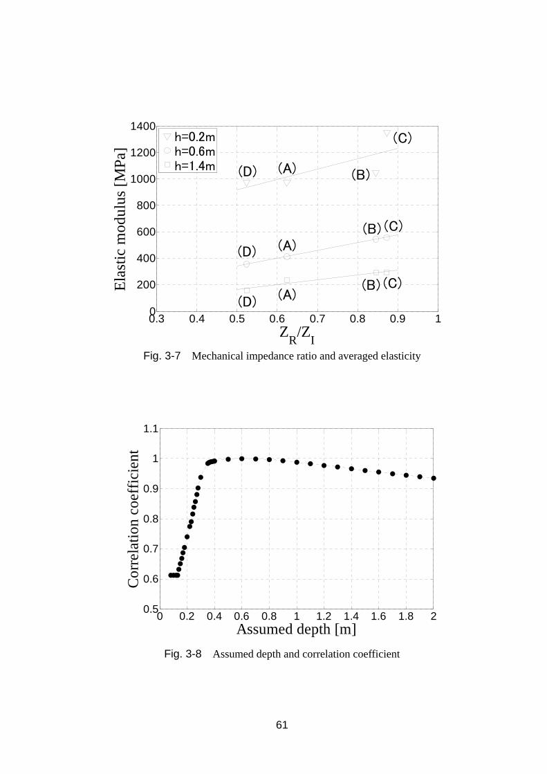
61

Fig. 3-7 Mechanical impedance ratio and averaged elasticity

Fig. 3-8 Assumed depth and correlation coefficient

0.3 0.4 0.5 0.6 0.7 0.8 0.9 10

200

400

600

800

1000

1200

1400

ZR

/ZI

Ela

stic

mod

ulus

[M

Pa]

h=0.2mh=0.6mh=1.4m (D) (B)(A)

(D) (A)(B)

(D) (A)(B) (C)

(C)

(C)

0 0.2 0.4 0.6 0.8 1 1.2 1.4 1.6 1.8 20.5

0.6

0.7

0.8

0.9

1

1.1

Assumed depth [m]

Cor

rela

tion

coe

ffic

ient

62

(3) Result and evaluation of impact sound

Time series of the sound recorded by normal and low frequency level meters when the

pavement of A-section is impacted is shown in Fig. 3-9 as an example. In the figure,

impact load together is also plotted. From this figure, it is observed that the wave by

normal level meter contains high frequency components more than that by low frequency

level meter which mainly records low frequency components. Because the contact sound

caused by attaching the hummer and pavement surface yields high frequency sound, it is

proper to use low frequency level meter which can focus on the low frequency sound

caused by surface vibration. Hereafter, record the sounds recorded by the low frequency

sound level meter are used to discuss and evaluate the model pavement.

Ten impact sounds for each model pavement are averaged and then analyzed to obtain

frequency components. Fig. 3-10 shows frequency spectrums of the impact sound from

each model pavement. In this figure, each spectrum is normalized. First, the peak around

105Hz is focused on. For all models, this dominant frequency can be identified in the

spectrum but the power at this frequency of D-section is smaller than the others. On the

basis of wavelet analysis for the impact sound, it was found that the sound with this

frequency occurs only at the moment of hitting. Thus it can be said this frequency relates

to the sound of hitting moment. Note that several factors affecting the sound such as voids

or roughness of surface may correspond to the higher frequencies.

Next, the peaks around 30Hz and 60Hz can be considered as the first and second

order vibration of pavement surface. However, it is difficult to identify the first order

dominant frequency of D-section pavement. It may be caused by the fact that the bearing

capacity of sub-grade at D-section is quite small and the first order dominant frequency

becomes lower than 20Hz which is beyond the range of low frequency sound level meter.

Regarding to dominant frequencies around 30Hz and 60Hz, A-section and C-section

pavement where sub-grade has almost identical bearing capacity yields almost identical

dominant frequencies. In the same trend, B-section pavement where sub-grade has lower

bearing capacity yields smaller dominant frequencies than those in A-section and

C-section pavement. Moreover, it can be seen that the second dominant frequency of

D-section pavement is much smaller than those of other pavement sections.

Therefore, the dominant frequencies of the impact sound may indicate the bearing

capacity or stiffness of pavement sub-grade.

63

Fig. 3-9 Impact sound from A-section pavement

Fig. 3-10 Frequency spectrum of impact sound

from each pavement section

-5

0

5

10

15

20D

ynam

ic lo

ad [

kN]

0 10 20 30 40 50-1

-0.5

0

0.5

1

Time [msec]Nor

mal

ized

Am

plit

ude

Normal sound level meterLow frequency sound level meter

0

0.5

1 30.3 65.0 106.7

0

0.5

1 105.0 58.0

22.0

0

0.5

1 64.134.2

103.8

Nor

mal

ized

PS

D

0 50 100 150 2000

0.5

1 41.3

108.0

Frequency [Hz]

A Section

B Section

C Section

D Section

64

3.3 Parametric analysis for impact sound using FEM

3.3.1 Outline of FEM and model analysis

For the next step, the effect of thickness and elastic modulus of each pavement layer on

the property of impacting sound is evaluated. Herein, because the dominant frequency of

impact sound includes that of the surface vibration , instead of evaluating the sound

directly the vibration of pavement surface is simulated and evaluated. First, numerical

model is built to represent impacting test and calibrated to have the identical trend

obtained in the test. Next, by using the numerical model, parametric study was conducted.

In this analysis, the thickness and properties of surface layer, base course, sub-base and

sub-grade which may affect the dominant frequency were varied. Note that time history

response analysis by modal superposition dynamics method was used to analyze the

response due to impact. Then, the displacement response was examined by

Fast-Fourier-Transform to find out the dominant frequencies of surface vibration.

This dynamic response analysis is done by ABAQUS[56] programming that is a wide

use soft of FEM analysis. The model has a half of effective width of pavement section

because of its symmetry. The bottom surface was perfectly fixed and the horizontal

displacements at the both sides were fixed. Note also that a symmetric model was

assumed with loading point in the middle of the axle, and a uniform material of each layer

in this analysis. In this situation, the difference of three-dimensional model and

two-dimensional model can be acceptable, and then two-dimensional analysis with plane

strain was conducted. In the analysis, sub-grade has 50 x 50 elements and the height of an

element in surface layer and base course is 5mm, and more elements are placed in the

middle that has stress concentration. Fig. 3-11 shows the numerical model of pavement.

The range of thickness and physical properties used in numerical analysis are shown in

Table 3-4. Note that Poisson’s ratio of each layer is assumed to be 0.35, and sub-grade

thickness has a constant value of 2770mm. In this table, actual properties obtained in the

experiment for A-section are also listed using parentheses.

To load the pavement model, 20kN uniform distribution load having 25mm length

corresponding to radius of the impact hammer was applied, and 3msec contact time of

rectangular wave was assumed by referring the recorded force in the experiment. Herein,

to match the spectrum of numerical analysis with the test value, critical damping constant

of each mode was set from 0.01 to 0.1.

65

Fig. 3-11 Numerical model pavement

Table 3-4 Physical properties employed in numerical analysis

Each layer Elastic modulus

[MPa]

Thickness

[mm]

Density

[kg/m3]

Surface layer t1 1000 ~ 4000

(2000)*

0 ~ 100

(30)* 2281

Base course t2 300 ~ 800

(500)*

50 ~ 400

(100)* 2161

Sub-base t3 100 ~ 600

(300)*

50 ~ 400

(100)* 1959

Sub-grade t4 5 ~ 250

(200)* 2770 2000

* : Thickness and elastic modulus of A-section pavement

66

3.3.2 Verification of the numerical model

To verify the numerical model, the time history recorded at A-section was used. Time

series data of impacting sound obtained by the experiment and the simulated

displacement response at the impacting point are shown in Fig. 3-12. In Fig. 3-13 their

frequency spectrum are also plotted. From the figure of time series, it is observed that the

displacement response of pavement surface still vibrates even after 10msec, but the

amplitude of impacting sound converges to zero after 20msec. This may be attributed to

the fact that the sound pressure caused by the surface vibration attenuates much faster

than that of the surface vibration and such small fluctuation cannot be recorded by sound

level meter. However it can be seen in the spectrum that the spectrum of the displacement

response has almost identical dominant frequency to that of impacting sound.

Therefore, it can be said that the numerical model is validated, and then this model is

used in the following parametric analysis.

3.3.3 Effect of each layer thickness on dominant frequency

In order to evaluate the effect of each layer thickness on the dominant frequency, herein

only surface layer thickness and base course, sub-base thickness are discussed, as

describe in the following.

(1) Effect of surface layer thickness on dominant frequency

To confirm the effect of the thickness of the surface layer, the other properties are fixed

but the thickness varies in the pavement of A-section. Fig. 3-14 shows the relationship

between surface layer thickness and the dominant frequency obtained by analyzing the

displacement response in numerical model. Note that there are two dominant frequencies

can be confirmed in the spectrum according to surface layers. In this figure, ☐ indicates

the frequency obtained by the impacting test results of A-section pavement, △ also

indicate the frequency in of the test of C-section pavement that has different thickness in

surface layer from A-section.

From the figure, it is found that there is no significant change in dominant frequencies

as the thickness varies, and that the actual values of frequency are almost identical to

those in numerical simulation.

67

Fig. 3-12 Time-series data of impacting sound and displacement response

Fig. 3-13 Frequency spectrum of impacting sound and displacement response

-1

-0.5

0

0.5

1A

mpl

itud

e [V

]

0 10 20 30 40 50-40

-20

0

20

Time [msec]

Am

plit

ude

[x10

-3 m

m]

Displacement response (analysis)

Impacting sound (experiment)

0

0.5

1

Nor

mal

ized

PSD

30.3 65.0

106.7

0 50 100 150 2000

0.5

1

Frequency [Hz]

Nor

mal

ized

PSD

31.1

69.3

Impacting sound (experiment)

Displacement response (analysis)

68

Fig. 3-14 Pavement thickness and dominant frequency (surface layer)

Fig. 3-15 Pavement thickness and dominant frequency (base course and sub-base)

0 10 20 30 40 50 60 70 80 90 100 10

20

30

40

50

60

70

80

90

Surface layer thickness [mm]

Fre

quen

cy [

Hz]

50/50100/100 200/150 300/300 400/40010

20

30

40

50

60

70

80

90

Base course/Sub-base [mm/mm]

Fre

quen

cy [

Hz]

69

(2) Effect of base course and sub-base thickness on dominant frequency

Next, to clarify the relationship between the thickness and dominant frequencies, the

dominant frequencies corresponding to different thickness of sub-base layer in the

standard pavement were obtained by numerical simulation. The results are shown in

Fig. 3-15. In this figure, ☐ indicates the actual values obtained in the impacting test for

A-section pavement, △ also indicates the actual value for B-section having different

base course thickness from that of A-section. Note that because the sub-grade stiffness of

B-section is different from that of A-section, the analysis result by the model with the

same sub-grade stiffness as that of B-section is also shown in the figure by ▲. From this

figure, even though there is a gap about 10Hz between the second order dominant

frequency of analysis and that of the actual value for B-section pavement, the other

results of analysis agree well with the actual values. When the second order dominant

frequencies are focused on, it is observed that the frequencies increase slowly as the

thickness of base course increases. But when the increment is small, the first order of

dominant frequency is almost identical. Therefore, it can be said that the effect of base

course and sub-base thickness on the dominant frequency is not significant.

Fig. 3-16 Elastic modulus and dominant frequency (surface layer)

1000 1500 2000 2500 3000 3500 400010

20

30

40

50

60

70

80

90

Elastic Modulus [MPa]

Freq

uenc

y [H

z]

70

Fig. 3-17 Elastic modulus and dominant frequency (base course)

Fig. 3-18 Elastic modulus and dominant frequency (sub-base)

300 400 500 600 700 80010

20

30

40

50

60

70

80

90

Elastic Modulus [MPa]

Freq

uenc

y [H

z]

100 200 300 400 500 60010

20

30

40

50

60

70

80

90

Elastic Modulus [MPa]

Freq

uenc

y [H

z]

71

3.3.4 Effect of each layer elastic modulus on dominant frequency

Next, to clarify the effect of elastic modules on the dominant frequencies, the dominant

frequencies were obtained by numerical simulation for the model with varying modulus

of surface layer, base course, sub-base as well as sub-grade, respectively. Fig. 3-16 ,

Fig. 3-17 and Fig. 3-18 show the dominant frequencies of displacement response at the

impact point in simulation when the elastic modulus of surface layer, base course and

sub-base of pavement varies, respectively. In these figures, ☐ indicates the actual values

obtained in the impact test for A-section pavement. From these figures, it is observed that

there the dominant frequencies of both the first and second order are almost identical as

the elastic modulus of surface layer, base course and sub-base increase.

On the other hand, the dominant frequency drastically varies when the elastic

modulus of sub-grade varies as shown in Fig. 3-19. In Fig. 3-20, the same relationship

but with square root of elastic modulus is shown. In these figures, △ indicates the actual

value in the impacting test for D-section pavement which has sub-grade elastic modulus

different from that of A-section pavement. From these figures, it is observed that there is

a linear relationship between the square root of sub-grade elastic modulus and the

dominant frequency. In addition, it is also clarified that the second order dominant

frequency obtained in the test is almost identical to that by numerical simulation for the

D-section having elastic modulus around 40MPa (√40 6.32). Because the first order of

dominant frequency in simulation is around 15Hz which is lower than 20Hz, the lower

limit recorded range of low frequency sound level meter, the first order dominant

frequency in the test was not able to be confirmed.

According to the result of numerical analysis, it can be said that the first and second

order of dominant frequency may have strong relationship with elastic modulus of

sub-grade pavement, and when the elastic modulus of sub-grade becomes small then the

dominant frequency also significantly decreases.

Thus, it can be said that the lower frequencies in vibration of pavement surface do not

depend much on the thickness or elastic modulus of surface layer and base course of

pavement, but it is strongly subject to the elastic modulus of sub-grade pavement.

Therefore, it can be said that the dominant frequency in the sound when the surface is

impacted may represent the elastic modulus of sub-grade such as poor ground sub-base or

pavement with underground space.

72

Fig. 3-19 Elastic modulus and dominant frequency (sub-grade)

Fig. 3-20 Square root of Elastic modulus and dominant frequency (sub-grade)

5 20 40 80 120 160 200 225 2500

10

20

30

40

50

60

70

80

Elastic Modulus [MPa]

Freq

uenc

y [H

z]

2 4 6 8 10 12 14 160

10

20

30

40

50

60

70

80

Square root of elastic modulus [MPa0.5]

Freq

uenc

y [H

z]

73

3.4 Evaluation procedure of pavement structures

In addition to road pavement surface, the structure of pavement also important to be

evaluated as the stiffness of pavement decreases due to the deterioration progresses.

Conventionally, FWD equipment is used to estimate stiffness-related parameters of

pavement and road bed. In this system, the deflection and reaction force of the pavement

is recorded when a weight is falling on the pavement. The testing device includes a

guided weight, deflection sensors and a load cell. However, there have some difficulties

in measurement due to something like insufficient maintenance budget.

Thus, in this study a simple system to evaluate road pavement structure in developing

country by using impact load and impact sound. From the above description, it was found

that mechanical impedance ratio from impact load could evaluate averaged elastic

modulus of pavement surface, and dominant frequencies of impact sound could evaluate

the stiffness of sub-grade. Therefore, the procedure of the evaluation system should be

followed by the flow as shown in Fig. 3-21.

Fig. 3-21 Evaluation procedure using impact load and sound

Impact load and impact

sound results

Impedance ratio>Standard value No need structural repairYes

Problem in

subgrade

Problem in

pavement surface

Dominant frequency>Standard value

No

No

Yes

Replastering of surface

layer or overlay

Improvement of

subgrade soil

74

3.5 Summary

In this chapter, to develop a very simple method for structural evaluation of road

pavement, fundamental study of both experimental test and numerical analysis were

carried out. By focusing on the relatively thin layers such as DBST, impact technique was

applied to evaluate the structural properties of pavement. The results from the study are

resumed as following.

(1) When the surface of pavement was impacted by impact hammer, it was found that

the averaged elastic modulus from the surface to some depth of pavement can be

evaluated by evaluating mechanical impedance ratio obtained by the waveform of

impacting load.

(2) From the frequency analysis for the impacting sound recorded in the impacting

test on model pavement, it was found that the dominant frequencies in sound were

almost identical when the thickness of surface layer or base course was different,

but the frequencies were significantly changed when the stiffness of sub-grade

was changed.

(3) From the result of FEM dynamic analysis representing the experiment, it was

found that dominant frequencies in the displacement response of pavement surface

are almost identical even with different thickness or elastic modulus of surface

layer and base course of pavement but the frequencies are drastically changed

when the elastic modulus of sub-grade is changed. Moreover, the dominant

frequency in the model with varying modulus of sub-grade is directly proportional

to the square root of elastic modulus.

Therefore, it can be said it is possible to evaluate the averaged elasticity of pavement

from the surface to some depth by evaluating the impacting load, and at the same time by

evaluating the first and second order of dominant frequency of impacting sound, it is also

possible to evaluate the stiffness of sub-grade of pavement. Thus, for pavement

management in developing country, structural condition of road pavement could be

evaluated easily by the proposed method. However, the above results are confirmed only

by assumed model pavement, and thus more future studies should be done at the field to

put it in practical use. Note that it should exploit this simple impacting method in PMS,

however, to apply such impedance ratio of impacting load and dominant frequencies of

impacting sound in PMS, it is necessary to clarify the relation between those indices with

FWD deflection.

75

Chapter 4 Development of a simple IRI

measurement system using a

motor bicycle for roughness

evaluation

4.1 General remarks

In maintenance of a road pavement, the longitudinal evenness is evaluated widely by

using International Roughness Index (IRI). IRI is an index introduced by World Bank in

1986, to evaluate longitudinal evenness of pavement and riding comfort. In order to

estimate IRI, there are 4 classes of system corresponding to their accuracy[32]. Among

these classes, class 3 is a system using vehicle responses for IRI estimation and is widely

used. In this class 3 system, normally some specific vehicle should be used. However, in

many developing countries, motor bicycles are most popular and available transportation

comparing with the other vehicles such as truck and passengers’ vehicles. Previous

studies for class 3 system have mainly focused on 4-wheel vehicles to use and motor

bicycles have never been used for IRI estimation.

Therefore in the study of this chapter, IRI estimation using the response of a motor

bicycle which is most available and cheap transportation in developing countries was

attempted. Because a motor bicycle can move on any path more freely than vehicles, the

bicycle should run on the inner wheel path (IWP) of a road to have consistency in the

other systems. Herein, the system estimated IRI using motor bicycle is proposed and

verified in the field tests. Note that principle of the proposed system is basically identical

to the measurement principle of VIMS[35], [36], which is also class 3 system using vehicle

responses.

4.2 Measurement principle

4.2.1 VIMS (Vehicle Intelligent Monitoring System)

VIMS[35], [36] is the abbreviation for Vehicle Intelligent Monitoring System, which is a

76

class 3 system using the acceleration response of a sprung mass (vehicle body) in a

vehicle. In this system, Quarter-Car model (QC model) is used for conversion from

acceleration to IRI. As shown in Fig. 4-1, QC model is a numerical model representing

one wheel of vehicle and is also used in the definition of IRI. The definition of IRI is an

integral of relative velocity of sprung and unsprung mass of the QC model ( ) with

specific properties by inputting road profiles in the form

1| |

/

(4-1)

where is evaluation distance (generally 200m), is running speed (80km/h),

and is response velocity of sprung and unsprung mass, respectively. Each parameter

of QC model in the definition is shown in Table 4-1. Herein, and is a mass of

sprung and unsprung mass of a model, respectively, and is spring constant of tire

and suspension respectively, and is damping coefficient of suspension.

In VIMS, first to build QC model of the measured vehicle installed with measuring

device ( ), hump test calibration is applied. In the hump test, a vehicle transcends

specific humps with constant speed of 20km/h to identify the features of the vehicle. Then,

the responses of and are calculated by inputting the road profile of some

actual road into each numerical model, transfer function ( / ), the ratio of those

power spectrums, is computed. Next, measurement vehicle is driven on the target road,

and then the acceleration response of a sprung mass of the vehicle is measured and the

root mean square ( ) is computed. After that, by multiplying RMS of the

measurement vehicle by the transfer function, RMS of the sprung mass acceleration of

can be obtained. Finally, can be computed on the basis of the linear

relationship between and of sprung mass acceleration response of as

given by

0.0578 0.089 (4-2)

The estimation flow from acceleration measurement to IRI computation is resumed in

Fig. 4-2. For more details about procedure of the system, please refer to the previous

study [35].

In addition, because 80km/h of driving speed is assumed in the definition of IRI,

when driving speed is different from 80km/h, it is necessary to adjust running speed of

to the practical speed in the step of building transfer function.

77

Fig. 4-1 QC model

Table 4-1 QC model parameters for IRI estimation

/ 6.0

/ 65.3

/ 63.3

/ 0.15

78

Fig. 4-2 IRI estimation flow by VIMS[35]

Running on

road surface

IRI estimation

Speed

V km/h

Vehicle sprung

mass acceleration

Identify

Vehicle mean power

/

mean power

IRI

Running over

a hump

Vehicle sprung

mass acceleration

Actual measured

profile

Linear relation between

RMS and IRI

Speed V km/h

Speed 80 km/h

QC identification

79

4.2.2 Principle of IRI estimation using a motor bicycle

In the estimation of IRI using a motor bicycle, QC model is also built to represent the

motor bicycle in the hump test and then transfer function is calculated using some known

profiles. Then to estimate IRI, RMS of the bicycle’s acceleration is obtained and

multiplied by the transfer function. In the case of standard VIMS the system using a

vehicle, an accelerometer is basically installed on sprung mass because it is simple and

the response of sprung mass is directly related to riding comfort. However, when it comes

to motor bicycles, it is not so difficult to install the accelerometer on the unsprung mass,

and thus all the positions such as suprung and unsprung mass at front and rear were

examined.

Finally, one location of the accelerometer will be determined by considering the result

of running test describing in section 4.4.2. Note that in actual motor bicycle, there are

also pitching movement and lateral movement to be considered in numerical model. But

in this study, because vertical movement is basically considered for IRI estimation,

simply spring-mass system model, QC model is used to represent the motor bicycle

response. To represent the complicated response of a motor bicycle, nonlinearity of

damping is considered[59] as shown in Fig. 4-3, in the form

/ 0

0/

(4-3)

Fig. 4-3 Nonlinearity of damping[59]

Tension

Compression

Velocity

(Compression)

Velocity

(Tension)

v-pp

Damping force

80

4.3 Measurement test

4.3.1 Measurement outline

Five different types of motor bicycle as shown in Fig. 4-5 were used and two

measurement tests were executed in this study. First is the hump test to identify the

fundamental feature of these five motor bicycles. And the other test is a running test to

confirm the measurement repeatability. During these measurement tests, four

accelerometers sprung and unsprung mass at front and rear are installed on the motor

bicycle. Note that for sprung mass accelerometer with 20m/s2 capacity, ARF-20A of

Tokyo Sokki Kenkyujo, is installed and accelerometer with 50m/s2 capacity, ARF-50A of

Tokyo Sokki Kenkyujo, is installed for unsprung mass. Illustration of the sensor locations

in motor bicycle is shown in Fig. 4-4.

(a) Front sprung (b) Front unsprung

(c) Rear sprung (d) Rear unsprung

Fig. 4-4 An example of accelerometers installation (M5)

81

M1 : Honda Super cub 90cc

M2 : Honda Icon 110cc

M3 : Suzuki Smash 110cc

M4 : Suzuki Axelo 125cc

M5 : Honda XL 250cc

Fig. 4-5 Five different types of motor bicycle

82

4.3.2 Hump test

In hump test, motor bicycle is run over a hump as shown in Fig. 4-7 with a constant

speed 20km/h, to obtain properties of the bicycle. In this process, QC model for the

bicycle is built. Besides the measurement, numerical simulation is also conducted to

identify the model. In this simulation, the configuration of hump as shown in Fig. 4-6 is

used as input profile, and the response of the model is obtained by using Newmark-b

method with 250Hz sampling. Herein, parameters such as , , and dumping

properties ~ , are calculated by assuming 1. For optimization, the simulated

waveform and the response waveform of measurement is compared in frequency domain,

and the parameters are determined by minimizing the error between them below than

11Hz. It is known that the responses of a vehicle at less than 2cycle/m in spatial

frequency[36] have much influence on IRI, and thus the frequencies less than 11Hz which

corresponds to 2cycle/m when the running speed is 20km/h, is focused on. Note that

herein genetic algorithm (GA) is applied in the optimal computation.

Fig. 4-6 Hump configuration

Fig. 4-7 Hump test

83

4.3.3 Running test

In running test, each motor bicycle runs on the same road surface. And then IRI estimated

from each motor bicycle is discussed and compared. For the running course, DBST

(Double Bituminous Surface Treatment) pavement in Phnom Penh city of Cambodia

about 1km as shown in Fig. 4-8 is selected. And three kinds of running speed are

considered, 30km/h, 40km/h and 50km/h. The condition of the road surface is relatively

well, and the IRI value is about 1.5 ~ 2.5m/km.

Fig. 4-9 shows IRI estimation results of the road surface by VIMS using the response

of a vehicle. Note that evaluation distance of IRI is 200m for both bicycle and vehicle, but

the running speeds for the vehicle are 30km/h, 40km/h, 50km/h, 60km/h and 80km/h, and

acceleration was recorded twice for each speed. Evaluation distance is shifted with 10m

(95%) overlap. In this figure, IRI is plotted at the center of evaluation distance. In the

figure, black line indicates the average of all estimations and the other lines indicate each

estimation result. From this figure, the difference among the cases is small and it is

known that the reproducibility of IRI is high enough for standard VIMS.

Detail discussion about the accuracy of VIMS, please refer to the previous study [36].

Thus, herein the result by standard VIMS using vehicle response is used for baseline to

evaluate IRI estimation by motor bicycle.

Fig. 4-8 Running course (Phnom Penh city)

84

4.4 Measurement results

4.4.1 Hump test results

The response of front unsprung mass of M2 motor bicycle is shown in Fig. 4-10 as an

example, and also the spectral density of the acceleration responses at all locations are

shown in Fig. 4-11. In this figure, the average of five times of measurement is also

drawn. The average value in spectral density is not an average of spectrum but a spectral

density of the averaged waveform. Because the dominant frequencies of a motor bicycle

movement are mainly below than 20Hz, the response is processed by 20Hz of low pass

filter.

First, the response of unsprung mass is discussed. From Fig. 4-11, it is observed that

spectrum has the peaks around 6Hz and 16Hz of front and rear unsprung mass,

respectively. The peak around 6Hz may correspond to a resonance point[59] of unsprung

mass assuming in QC model. And the peak around 16Hz may correspond to an impulse

waveform at the hump. In the case that running speed is 20km/h, about 5.5m/s, the

impulse width is 0.054 second when it passes over a hump of 0.3m, and then theoretically

about 18.5Hz of response will occur. Especially, as for unsprung mass the response at this

frequency becomes large because the imposed displacement by hump is dominated.

Next, the response of sprung mass is discussed. For the response of front sprung mass,

it is observed that the spectrum has the peak around 3Hz which cannot be confirmed in

that of unsprung mass. Also for rear sprung mass, even though it is small there is a peak

around 3Hz in the spectrum. This peak may correspond to a resonance point of sprung

mass. In addition, it is also observed that the spectrum of front and rear unsprung mass

has the peak around 6Hz which may correspond to a resonance point of unsprung and

can be also confirmed in the spectrum of sprung mass. Thus, it can be said that the

movement of rear unsprung mass is almost identical to that of front unsprung mass, but

the movement of rear sprung mass is different from that of front sprung mass. This may

be attributed to the fact that movement of a rider directly affects the sprung mass

movement and also of the location of accelerometer is not adequate to capture the

movement. Thus the response of rear sprung mass recorded by the accelerometer may

represent not only the bicycle movement but also other attachments. Note that in the

spectrum of front and rear sprung mass , the peak about 10 ~ 12Hz can be confirmed, and

this peak may correspond to a movement of motor bicycle body due to the pitching that

cannot be simulated by QC model.

The trends described above can be also found in the other motor bicycles except for

M1 motor bicycle. In M1 motor bicycle, front wheel uses front fork of bottom link type,

where the suspension is connected right above with the wheel, and the movement of front

85

Fig. 4-9 IRI estimation results by VIMS

Fig. 4-10 An example of the response from hump test

(M2 front unsprung mass)

86

Fig. 4-11 Spectral density of each response of M2

87

fork is almost identical to that of sprung mass. For the other motor bicycles, they adopt

the telescopic type suspension system, and the movement of front fork is identical to that

of unsprang mass which can be correctly captured by the installed sensor. Thus, it is

observed that the response of M1 front unsprung mass is different from those of the other

motor bicycles. The spectral densities of front unsprung mass and sprung mass in M1 are

shown in Fig. 4-12. In M1 motor bicycle, due to the structure of suspension system, the

response of unsprung mass is nearly equal to that of sprung mass. Besides M1, M5 is also

different from that of other motor bicycles, but there is no remarkable difference from the

others.

Next, the identification of QC model for M2 bicycle through the hump tests is

discussed. The response of front unsprung and sprung mass of M2 by the identified QC

model is shown in Fig. 4-13, respectively, and their spectral densities are shown in

Fig. 4-14. Note that to identify the parameter of QC model, the power spectrum below

than 11Hz which is sensitive to IRI is optimized till the error over the range of 2cycle/m

becomes small. From this figure, it is observed that the simulated spectrum agrees well

with that of the measurement in the range up to 20Hz for unsprung mass. This is

attributed to the fact that in unsprung mass response the input of imposed displacement by

hump and elastic behavior of unsprung mass is dominant. On the other hand, for sprung

mass, although long cycle around 3Hz of sprung mass resonance point can be simulated,

but the frequencies over 6Hz including resonance point of unsprung mass cannot be

simulated well. This may be caused by the fact that these frequencies include

three-dimensional vibration which cannot be expressed by QC model such as body

pitching. This feature was also confirmed in the response of sprung mass and unsprung

mass on the rear. From the viewpoint of QC model fitting, the reproducibility of unsprung

mass is high and useful. But form the viewpoint in IRI conversion, sprung mass is not

abandon because they simulate the resonance mode of sprung mass which much affects

IRI estimation.

The transfer function of QC models from the identified QC model to the QC model in

definition is shown in Fig. 4-15. Note that horizontal axis shows the special frequency

(cycle/m) that can be determined by each speed. From this figure, it is observed that

different transfer functions are constructed corresponding to each speed. It is also

observed that difference becomes large as the frequency decreases below than 0.5cycle/m,

and the lower speed have larger value. In the process of IRI conversion by VIMS, 0.3Hz

of low pass filter on special frequency is applied[36], to emphasis on the response around

the resonance point of sprung mass movement , and to reduce the effect of speed. In the

system for motor bicycles, 0.3Hz of special filter is also applied.

88

(a) Front unsprung

(b) Front sprung

Fig. 4-12 Spectral density of the response of M1

89

(a) Front unsprung

(b) Front sprung

Fig. 4-13 The response from QC model

90

(a) Front unsprung

(b) Front sprung

Fig. 4-14 Spectral density of the response from QC model

91

(a) Front unsprung

(b) Front sprung

Fig. 4-15 The transfer function between and

92

4.4.2 Running test results

The result of IRI estimation by the response of M2 bicycle is shown in Fig. 4-16. In this

figure, black line denotes the average value by standard VIMS using a vehicle passing on

the same path. From Fig. 4-16(a)(b), in the case using response of front wheel, it is

found that the results of sprung and unsprung mass agree well with the result of vehicle.

Especially for sprung mass, the result over the distance up to 400m has very good

agreement with IRI estimated by vehicle, and for all distance the repeatability is high or

in other words, the dispersion of the results is small. For the distance over 400m, the

result is different from IRI by vehicle about 0.4m/km, but when considering that there is a

dispersion around 0.3m/km even in the estimation of IRI by vehicle, and thus it can be

said that the obtained result is well. The errors in the sprung mass may be caused by the

fact that the effect of 6Hz mode cannot be expressed by QC model. Especially, because

the response is filtered by low-pass filter of 0.3cycle/m in special frequency, the mode

having the frequencies higher than this frequency may be ignored in the estimation.

From Fig. 4-16(c)(d), in the case of rear wheel, it is found that the results of sprung

mass are much different from the value by vehicle. For unsprung mass, although the

result agrees with the value of vehicle in the case of 50km/h, the result depends much on

the velocity and much deviation is found. This may be caused by the direct effect of

driving force. As F for the response of rear sprung mass, because of improper sensor

location, the response may not be captured properly. Thus, when the accelerometer is

properly located, the accuracy of IRI estimation by rear sprung mass could be improved.

Next, the IRI estimated by the response of front sprung mass of all motor bicycles are

discussed. The IRI estimation results by the response of front sprung mass in all bicycles

are shown in Fig. 4-17. From these figures, the results of each motor bicycle are mostly

equal to the IRI estimated by vehicle, except for M5. This may be caused by the

difference of between the assumed and actual velocities because the difference in M5

reaches about 25% but those of the other bicycles are around 10%. Thus on the basis of

actual speed confirmed by GPS, the average speed over the evaluated section is obtained

and used for estimation instead of the assumed speed. Then, the result of IRI estimated by

using actual speed is shown in Fig. 4-18. From this figure, it is found that the estimation

of IRI is drastically improved by using actual speed.

Therefore, by using the response of front sprung mass of each motor bicycle, it can be

said that the IRI estimated by motor bicycles agree well with that by the vehicle. When

the assumed speed is much different from the actual speed, it is necessary to reconstruct a

transfer function corresponding to the actual speed because speed effect cannot be

ignored.

93

Fig. 4-16 The results of IRI estimation using each response of M2

94

Fig. 4-17 IRI estimation results of each motor bicycle

95

Fig. 4-18 IRI estimation results after correcting speed

4.5 Summary

In this chapter, to develop a very simple method to evaluate the evenness of road surface

pavement using the response of motor bicycle, five different types of motor bicycle were

used. Together with clarifying the response characteristic in the hump test, the accuracy of

IRI estimation by constant speed running is also discussed. The followings are obtained in

this study:

(1) Four accelerometers are set on front, rear sprung and those of mass unsprung of a

motor bicycle, respectively, and the responses of them when the bicycle ran over a

hump is clarified. As a result, it was found in the unsprung mass response that

there are two response peaks of unsprung mass resonance point and a point

correspond to pulse input duration, and in the sprung mass response it is also

found that the response of front wheel contains sprung mass resonance point

clearly but that of rear wheel does not.

(2) To identify the characteristics of a motor bicycle, the response when the bicycle

ran over a hump is simulated by using QC model, using GA to identify the

parameter. Herein, the optimization was executed to lessen the error in the power

spectrum under 11Hz between the assumed and actual responses. As a result, it

96

was found that the response of unsprung mass can be simulated even in high

frequency range. However, the sprung mass response simulated does not agree

with the actual over 6Hz because the effect of body motion such as pitching

cannot be considered in QC model.

(3) IRI estimated from the response of each installation point was compared in a

motor bicycle. As a result, it was found that the IRI estimated by front sprung

mass almost agrees with that by vehicle response. For rear sprung mass, because it

is difficult to install accelerometer properly, IRI estimation cannot be attained by

the rear response.

(4) For M5 motor bicycle, as the assumed speed confirmed by the speed meter

mounting on motor bicycle is greatly different from the actual speed confirmed by

GPS, and thus the result by M5 was drastically improved by adjusting the velocity

in calculation process to estimate IRI.

Herein, the estimation method of VIMS was applied to a motor bicycle, and the

feasibility of IRI estimation using a motor bicycle response was discussed. As the result,

it is found that motor bicycles which are much available in developing countries, can be

used for IRI estimation to have almost identical accuracy to that by a vehicle when the

acceleration of front sprung mass is evaluated. However, in the range between 30km/h to

50km/h, because the effect of speed change is large and cannot be ignored, the transfer

function should be built by using actual speed which can be confirmed by GPS. Note that

the obtained IRI values could be applied in PMS directly.

97

Chapter 5 Evaluation of actual live loads

using a Bridge Weigh-In-Motion

technique

5.1 General remarks

Many Asian countries have been growing rapidly and expanded their possibility in

economics for recent years. Associated with this growth, infrastructures such as road

network, bridge, tunnel and highway were needed, and those structures have been built by

means of foreign aids or by themselves. Roads and bridges must be designed to match

their performance to the requirements, i.e., their bearing capacities are expected to resist

the design loads. In reality, however, unexpected over-loads apply to the bridges and

roads, and the overloads sometimes transcend their limitation because the trucks try to

carry the loads as much as possible (sometimes almost impossible) to increase their

transport efficiency. Such overloaded vehicles are often found in Asian countries and

officially they are not allowed by the regulation. In some cases, overloaded vehicles are

unofficially permitted by the police officers who do not understand its seriously harmful

effect on infrastructures. Mostly overloaded vehicles move over the structures at night

when the police officers are not in service.

When the applying load doubles, fatigue damage is 8 times as large in steel members

of a bridge, 16 times as large in concrete slab of a bridge or pavement of a road. Thus,

actual situation of applying loads should be clear and considered in maintenance of the

infrastructures.

In addition to this serious situation, sometimes live load model itself is not adequate

for the current situation because the assumed live load in design does not agree with the

actual loads. As is often the case in Asian countries, AASHTO, AUSROADS,

EUROCODE and other dominant codes are often adopted for the design of infrastructures.

These codes have been applied by modifying their design loads but sometimes the traffic

data is not available or, even if the data is available it may not reflect the current situation

because the traffic investigation was done before their economic development.

In Thailand, mainly they have adopted the codes according to AASHTO: the design

loads are modified to match the actual situation in Thailand, on the basis of the

fundamental vehicle models in AASHTO. However, the traffic investigation on current

98

weights of vehicles in nationwide scale has been seldom conducted. Thailand is one of

the cities in Asian countries where its economic has been growing rapidly and is an

appropriate model for comparison with design and actual live load. Therefore in the study

of this chapter, the effect of applying load on pavement fatigue is evaluated when actual

live load is considered instead of design on the basis of current traffic data by Bridge

Weigh-In-Motion in Bangkok city, Thailand.

5.2 Bridge Weigh-In-Motion

5.2.1 Principle of Bridge WIM

Bridge WIM is a system to estimate the live load applying to a bridge by analyzing its

responses. Several methods have been proposed so far, but we adopted the methods based

on the strain response of main girder which is originally proposed by Moses (1979)[57]. In

his theory, the axle load can be estimated by minimizing the residual error between the

influence line obtained by the measured stains and that by unknown load. In this system,

the position of axle load must be known beforehand to conduct the least square method,

and thus originally optical switch was used for axle detection. In our research, to

distinguish each axle the response of concrete slab is used because the response of

concrete slab is more sensitive than that of main girder. As can be seen in Fig. 5-1, two

sensors on the slab are installed away from each other in one stream line. Thus the wheel

base (distance of axles) and velocity can be recognized by using the response lag between

these two sensors, because each peak corresponds to an axle load (see Fig. 5-2).

Now the strain response of the main girder at the center span due to an axle load Pi is

given by

2 (5-1)

where is section modulus and is elastic modulus, is also defined as

0 /2 /2 (5-2)

where is a span length and is the position of from the support. Now let us

assume that the time when the first axle enters the bridge is zero and also the time when

the last axle exits the bridge is . With the time increment of ∆ , is equal to ∆

99

where is the number of data. When the load moves with constant velocity, , the

position of can be replaced by the time with the distance from the first to th axle,

, ( ). Then the total stain response at the center span, , by a vehicle

with axles can be expressed as

EZ2

(5-3)

Then we can estimate each by minimizing the errors between measured and

calculated values using least square method as follows:

(5-4)

where is measured strain and denotes the th time period. The monitored

bridge has four main girders and the gauges were installed on the outer two girders to

obtain the response corresponding to each stream. After the calibration to determine EZ

in equation (5-3), the system can estimate the axle loads. Note that the identification of

the types of vehicles is done by the theory developed in reference [58], and in general the

estimation error of the system is about 10% for total weight and more than 20% for axle

load.

Fig. 5-1 Layout of Bridge WIM

100

Fig. 5-2 Axle recognition by the responses of two strain sensors on concrete slab

5.2.2 Monitored Bridge

The monitored bridge for Bridge WIM in Thailand is one of the flyovers crossing the

main roads, which are located in the center area of Bangkok city. As shown in Fig. 5-3,

the monitored section has two superstructures which are independent each other on the

piers of P3 and P4. The superstructure is a steel concrete composite bridge with two steel

main girders and pre-cast concrete slabs. Thus we installed two independent Bridge WIM

systems on them. Layout of the sensor installation is shown in Fig. 5-4. In this figure, S1

and S2 denotes the sensor on the slab for axle detection while M1 and M2 denotes the

sensor on the bottom flange of main beams to detect the bending moment at the center

span. Note that the strain at the center is averaged by two responses obtained both

flanges.

Fig. 5-3 Monitored bridge: two independent superstructures stay on common piers

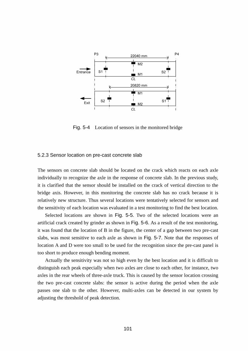
101

Fig. 5-4 Location of sensors in the monitored bridge

5.2.3 Sensor location on pre-cast concrete slab

The sensors on concrete slab should be located on the crack which reacts on each axle

individually to recognize the axle in the response of concrete slab. In the previous study,

it is clarified that the sensor should be installed on the crack of vertical direction to the

bridge axis. However, in this monitoring the concrete slab has no crack because it is

relatively new structure. Thus several locations were tentatively selected for sensors and

the sensitivity of each location was evaluated in a test monitoring to find the best location.

Selected locations are shown in Fig. 5-5. Two of the selected locations were an

artificial crack created by grinder as shown in Fig. 5-6. As a result of the test monitoring,

it was found that the location of B in the figure, the center of a gap between two pre-cast

slabs, was most sensitive to each axle as shown in Fig. 5-7. Note that the responses of

location A and D were too small to be used for the recognition since the pre-cast panel is

too short to produce enough bending moment.

Actually the sensitivity was not so high even by the best location and it is difficult to

distinguish each peak especially when two axles are close to each other, for instance, two

axles in the rear wheels of three-axle truck. This is caused by the sensor location crossing

the two pre-cast concrete slabs: the sensor is active during the period when the axle

passes one slab to the other. However, multi-axles can be detected in our system by

adjusting the threshold of peak detection.

102

Fig. 5-5 Details of installed sensors

Fig. 5-6 Artificial crack by grinder on concrete slab

Fig. 5-7 The responses of the sensors at the gap between slabs for the identical vehicle

-10

0

10

20

30

0 1 2 3 4 5 6 7 8 9 10

Str

ain,

Time, sec

B: Gap (center)C: Gap (side)

103

5.2.4 Calibration

To determine the EZ in the equation (5-1) and (5-3), 3-axle truck (the10-wheels truck)

whose axles were measured by truck scale passed the monitored section. Detailed

information for the truck is shown in Fig. 5-8. Note that “actual” values in the table

denote the values measured by other system.

Two different velocities were assumed and three runs were conducted for each

velocity but only one truck was used for this calibration due to a site limitation. The

coefficient was determined by the first run of low velocity and this coefficient was

verified by the other trials. The estimated values and the actual loads measured by a truck

scale are shown in the Table 5-1. Note that Ent. and Exit in the table denotes the lane of

Entrance and Exit, respectively. Note also that the systems for Entrance lane and Exit lane

are independent each other. From this table, it is clarified the system for Exit has higher

accuracy than that for Entrance because the data obtained in Entrance lane contains

significant noise. The estimation error of the total weight is less than 1% for both lanes,

while the error of each axle becomes around 20% for Exit lane. However, although the

estimated axial loads are not accurate much, total amounts of the vehicle weight estimated

by both systems are almost identical to that obtained by static measurement.

Table 5-1 Estimated values of the reference truck after the calibration

Case Direction Gross Velocity P1 P2 P3 AX1 AX2

kN km/h kN kN kN m m

Actual - 245.8 0 54.1 100.7 90.9 3.63 1.35

1 Ent. 246.0 16.3 9.7 118.1 118.1 3.70 1.24

2 Exit 245.1 22.8 57.3 93.9 93.9 3.70 0.90

3 Ent. 252.2 17.1 2.5 124.9 124.9 3.77 1.22

4 Exit 247.5 23.1 56.4 95.6 95.6 3.78 0.93

5 Ent. 255.3 18.3 0.0 127.6 127.6 3.75 1.22

6 Exit 253.9 19.8 69.7 92.1 92.1 3.89 1.26

7 Ent. 243.7 39.7 29.2 107.2 107.2 3.80 1.27

8 Exit 245.4 41.7 75.9 84.8 84.8 3.68 1.22

9 Ent. 247.1 39.5 31.6 107.7 107.7 3.79 1.10

10 Exit 245.8 42.8 73.5 86.1 86.1 3.63 1.19

11 Ent. 245.7 37.0 21.8 111.9 111.9 3.83 1.16

12 Exit 245.8 42.7 73.7 86.0 86.0 3.67 1.16

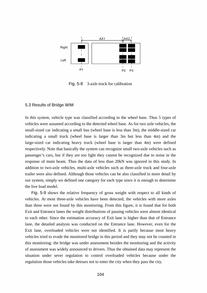
104

Fig. 5-8 3-axle truck for calibration

5.3 Results of Bridge WIM

In this system, vehicle type was classified according to the wheel base. Thus 5 types of

vehicles were assumed according to the detected wheel base. As for two axle vehicles, the

small-sized car indicating a small bus (wheel base is less than 3m), the middle-sized car

indicating a small truck (wheel base is larger than 3m but less than 4m) and the

large-sized car indicating heavy truck (wheel base is larger than 4m) were defined

respectively. Note that basically the system can recognize small two-axle vehicles such as

passenger’s cars, but if they are too light they cannot be recognized due to noise in the

response of main beam. Thus the data of less than 20kN was ignored in this study. In

addition to two-axle vehicles, multi-axle vehicles such as three-axle truck and four-axle

trailer were also defined. Although those vehicles can be also classified in more detail by

our system, simply we defined one category for each type since it is enough to determine

the live load model.

Fig. 5-9 shows the relative frequency of gross weight with respect to all kinds of

vehicles. At most three-axle vehicles have been detected, the vehicles with more axles

than three were not found by this monitoring. From this figure, it is found that for both

Exit and Entrance lanes the weight distributions of passing vehicles were almost identical

to each other. Since the estimation accuracy of Exit lane is higher than that of Entrance

lane, the detailed analysis was conducted on the Entrance lane. However, even for the

Exit lane, overloaded vehicles were not identified. It is partly because most heavy

vehicles tried to evade the monitored bridge in this period and they may not be counted in

this monitoring: the bridge was under assessment besides the monitoring and the activity

of assessment was widely announced to drivers. Thus the obtained data may represent the

situation under sever regulation to control overloaded vehicles because under the

regulation those vehicles take detours not to enter the city when they pass the city.

105

Fig. 5-10 shows the number of the vehicles passing this monitored bridge for one

week in the Exit lane. In this figure, the contribution of each type is also illustrated. From

this figure, it is found that the large sized car was dominant in this traffic. Note that total

number of vehicle on day 5 and day 6 are smaller than the other days because these days

were Saturday and Sunday.

Fig. 5-11 shows the relative frequencies of four vehicle types respectively. As for the

small-sized and middle-sized car, the distribution shapes are close to log-normal

distribution and the averages of gross weight are 46.3kN and 72.3kN, respectively. As for

the large-sized car, two main peaks are recognized in the distribution that can be fitted by

two different log-normal distributions. For safety reason, the second distribution with

larger average was adopted for representative herein and the average was 164.3kN. The

average of three-axle vehicles was not reliable because the sampling number is too small

for these two cases. But in this study we adopted the simple average values to represent

this type, and the average values were 178.0kN.

Fig. 5-9 Relative frequency of gross weight in Exit and Entrance lanes

Fig. 5-10 Time series of passing vehicles according to the vehicle type (Exit lane)

0.00

0.01

0.02

0.03

0.04

0.05

0.06

0.07

0.08

0 50 100 150 200 250 300

Rel

ativ

e fr

eque

ncy

Weight, kN

ExitEntrance

0

5

10

15

20

25

1 2 3 4 5 6 7 8Day

Nu

mb

er

of v

eh

icle

s

Small-sized car (2 axles) Middle-sized car (2 axles)Large-sized car (2 axles) 3 axle-truck

106

Fig. 5-11 Relative frequency of gross weight (according to the types of vehicles)

0.00

0.05

0.10

0.15

0.20

0 50 100 150 200 250 300

Rel

ativ

e fr

eque

ncy

Weight, kN

Small-sized car

0.00

0.02

0.04

0.06

0.08

0.10

0.12

0 50 100 150 200 250 300

Rel

ativ

e fr

eque

ncy

Weight, kN

Middle-sized car

0.00

0.01

0.02

0.03

0.04

0.05

0.06

0 50 100 150 200 250 300

Rel

ativ

e fr

eque

ncy

Weight, kN

Large-sized car

0.00

0.02

0.04

0.06

0.08

0.10

0.12

0.14

0.16

0 50 100 150 200 250 300

Rel

ativ

e fr

eque

ncy

Weight, kN

3 axle-truck

107

5.4 Comparison of actual and design load affecting fatigue deterioration of road

pavement

5.4.1 Daily five tons conversion axles number

It is known that fatigue of pavement (cracking) increases in proportion to the fourth

power of applying load. In design of pavement to determine the thickness of layers, an

equivalent live load is used to consider such an effect. In Japan, daily five tons conversion

axles number[37] is used to reflect the difference of various kinds of vehicles.

Daily five tons (49kN) conversion axles number can be calculated by

49 (5-4)

where (kN) and are representative values of axle load and axles number

respectively, and those values can be obtained from Table 5-2.

Table 5-2 Axle load range and Representative values[37]

Axle load range Representative values Axles number

~ 9.8 kN = 4.9

9.8 ~ 19.6 kN = 14.7

19.6 ~ 29.4 kN = 24.5

29.4 ~ 39.2 kN = 34.3

39.2 ~ 49.0 kN = 44.1

49.0 ~ 58.8 kN = 53.9

58.8 ~ 68.6 kN = 63.7

68.6 ~ 78.5 kN = 73.5

78.5 ~ 88.3 kN = 83.3

88.3 ~ 98.1 kN = 93.1

98.1 ~ 117.7 kN = 107.8

117.7 ~ 137.3 kN = 127.5

137.3 kN ~ = 147.1

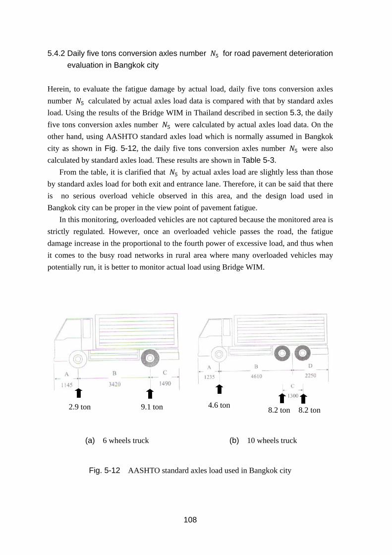
108

5.4.2 Daily five tons conversion axles number for road pavement deterioration

evaluation in Bangkok city

Herein, to evaluate the fatigue damage by actual load, daily five tons conversion axles

number calculated by actual axles load data is compared with that by standard axles

load. Using the results of the Bridge WIM in Thailand described in section 5.3, the daily

five tons conversion axles number were calculated by actual axles load data. On the

other hand, using AASHTO standard axles load which is normally assumed in Bangkok

city as shown in Fig. 5-12, the daily five tons conversion axles number were also

calculated by standard axles load. These results are shown in Table 5-3.

From the table, it is clarified that by actual axles load are slightly less than those

by standard axles load for both exit and entrance lane. Therefore, it can be said that there

is no serious overload vehicle observed in this area, and the design load used in

Bangkok city can be proper in the view point of pavement fatigue.

In this monitoring, overloaded vehicles are not captured because the monitored area is

strictly regulated. However, once an overloaded vehicle passes the road, the fatigue

damage increase in the proportional to the fourth power of excessive load, and thus when

it comes to the busy road networks in rural area where many overloaded vehicles may

potentially run, it is better to monitor actual load using Bridge WIM.

(a) 6 wheels truck (b) 10 wheels truck

Fig. 5-12 AASHTO standard axles load used in Bangkok city

2.9 ton 9.1 ton 4.6 ton8.2 ton 8.2 ton

109

Table 5-3 Daily five tons conversion axles number in Bangkok city

Each lane By actual axles load By standard axles load

Exit lane 1202 1235

Entrance lane 1039 1325

5.5 Summary

In this chapter, to evaluate the live load in Bangkok city, Bridge Weigh-In-Motion was

conducted for two weeks as a simple monitoring system, and then fatigue effect by actual

load was evaluated. Finally the following summary can be drawn from the results.

(1) In the Bridge WIM system using the composite bridge with precast slabs, the

sensors for axle detection should be installed on the gap between the precast slabs

to clearly identify the axle in the response. It is also confirmed that the algorithm

to recognize the type of vehicle can be applied to the traffic in Bangkok.

(2) As a result of monitoring, mostly heavy trucks with two axles are dominant

vehicles in the monitored bridge for the monitored period, and no overloaded

vehicle was observed in the monitored period. However, the monitored traffic may

not represent normal situation since the traffic might be regulated unofficially, and

it is better to capture the traffic in the other area.

(3) Finally it is found that the obtained daily five tons conversion axles number is

slightly less than that of AASHTO standard axles loading, and it is proper to use

the design load in design as well as maintenance of pavement. However, it is still

necessary to apply Bridge WIM as a simple live load monitoring, to know the

actual loads for pavement deterioration evaluation in the area where much of

overload vehicles potentially run.

110

111

Chapter 6 Conclusions

The intention in this study is the development a very simple method of structural

evaluation, roughness evaluation, live load evaluation and deterioration prediction for

road pavement management in developing country that face extremely on limitation of

budget allocated for the maintenance/repair/renewal of infrastructures. First, in Chapter 2,

the prediction behavior of some IRI prediction models are examined in order to find out

the most simple and available model adequate for pavement condition evaluation. Then,

the simple method of structural pavement evaluation and pavement roughness evaluation,

are developed in Chapter 3 and 4 respectively. Finally, in Chapter 5, the evaluation of

actual live load on the basis of current traffic data by Bridge Weigh-In-Motion as a simple

system for live load monitoring in Bangkok city, Thailand was studied. The following

conclusions are obtained in this study:

In Chapter 2, as in most developing countries such as Cambodia, the information

used for the pavement deterioration prediction seems insufficient and hard to acquire.

Then in this study, a very simple prediction model for Cambodian national road pavement

roughness is developed by using only the data of IRI, FWD and heavy vehicle traffic.

Herein five prediction models of HDM-4, LTPP, exponential equation, neural network

and Markov model are considered and discussed. The actual data of all 1-Digit

Cambodian national roads are used to build the models, and the actual data in year 2011

of national roads No.5 are used to examine the models. Besides the prediction, the

influence of several factors on the rate of IRI increment was also evaluated. The main

results from the study are resumed as following.

(1) By evaluating the influence of several factors on the rate of IRI increment, it was

found that IRI increment strongly depends on IRI value itself but the other factors

such as FWD deflection, structural number, are not significant.

(2) For the prediction by HDM-4 model, the necessary factors such as cracking,

rutting and potholing are not considered herein. This neglect may lead to smaller

values than the actual measured values when the IRI is high. Also in LTPP model,

almost all the values of IRI are underestimated.

(3) In the exponential model determined by actual surveyed data, it is found that the prediction result agrees well with the actual values. Neural network model also shows good agreement with the actual values but the error becomes large when the IRI value is over 5m/km.

112

(4) In Markov model by averaging operation, even though several influence factors

can be considered, the error is larger than that by enumeration method due to the

lack of the number of data.

(5) Finally it is clarified that FWD deflection and traffic information are significant

in the IRI prediction, and that the result predicted by exponential model can yield

the smallest error than that of the other models

Therefore, for Cambodian national roads No.5 where the data is limited, IRI value can

be predicted well by using exponential equation model. Moreover, because the

exponential model is built by using all the data of 1-Digit national roads, it is possible to

apply this prediction model to the other national roads. On the other hand, the other

models that have not enough input parameters can be possibly used also for IRI prediction,

however the error becomes large when the value of IRI is large. Note that in the future

when road pavement is properly maintained and the necessary input data is given with

high reliability, the other models might be express higher prediction performance. So it is

very important to collect the data regularly at the field site.

In Chapter 3, to develop a very simple method for structural evaluation of road

pavement, fundamental study of both experimental test and numerical analysis were

carried out. By focusing on the relatively thin layers such as DBST, impact technique was

applied to evaluate the structural properties of pavement. The results from the study are

resumed as following.

(1) When the surface of pavement was impacted by impact hammer, it was found that

the averaged elastic modulus from the surface to some depth of pavement can be

evaluated by evaluating mechanical impedance ratio obtained by the waveform of

impacting load.

(2) From the frequency analysis for the impacting sound recorded in the impacting

test on model pavement, it was found that the dominant frequencies in sound were

almost identical when the thickness of surface layer or base course was different,

but the frequencies were significantly changed when the stiffness of sub-grade

was changed.

(3) From the result of FEM dynamic analysis representing the experiment, it was

found that dominant frequencies in the displacement response of pavement surface

are almost identical even with different thickness or elastic modulus of surface

layer and base course of pavement but the frequencies are drastically changed

when the elastic modulus of sub-grade is changed. Moreover, the dominant

frequency in the model with varying modulus of sub-grade is directly proportional

to the square root of elastic modulus.

113

Therefore, it can be said it is possible to evaluate the averaged elasticity of pavement

from the surface to some depth by evaluating the impacting load, and at the same time by

evaluating the first and second order of dominant frequency of impacting sound, it is also

possible to evaluate the stiffness of sub-grade of pavement. Thus, for pavement

management in developing country, structural condition of road pavement could be

evaluated easily by the proposed method. However, the above results are confirmed only

by assumed model pavement, and thus more future studies should be done at the field to

put it in practical use.

In Chapter 4, to develop a very simple method to evaluate the evenness of road

surface pavement using the response of motor bicycle, five different types of motor

bicycle were used. Together with clarifying the response characteristic in the hump test,

the accuracy of IRI estimation by constant speed running is also discussed. The

followings are obtained in this study:

(1) Four accelerometers are set on front, rear sprung and those of mass unsprung of a

motor bicycle, respectively, and the responses of them when the bicycle ran over a

hump is clarified. As a result, it was found in the unsprung mass response that

there are two response peaks of unsprung mass resonance point and a point

correspond to pulse input duration, and in the sprung mass response it is also

found that the response of front wheel contains sprung mass resonance point

clearly but that of rear wheel does not.

(2) To identify the characteristics of a motor bicycle, the response when the bicycle

ran over a hump is simulated by using QC model, using GA to identify the

parameter. Herein, the optimization was executed to lessen the error in the power

spectrum under 11Hz between the assumed and actual responses. As a result, it

was found that the response of unsprung mass can be simulated even in high

frequency range. However, the sprung mass response simulated does not agree

with the actual over 6Hz because the effect of body motion such as pitching

cannot be considered in QC model.

(3) IRI estimated from the response of each installation point was compared in a

motor bicycle. As a result, it was found that the IRI estimated by front sprung

mass almost agrees with that by vehicle response. For rear sprung mass, because it

is difficult to install accelerometer properly, IRI estimation cannot be attained by

the rear response.

(4) For M5 motor bicycle, as the assumed speed confirmed by the speed meter mounting on motor bicycle is greatly different from the actual speed confirmed by GPS, and thus the result by M5 was drastically improved by adjusting the velocity in calculation process to estimate IRI.

114

Herein, the estimation method of VIMS was applied to a motor bicycle, and the

feasibility of IRI estimation using a motor bicycle response was discussed. As the result,

it is found that motor bicycles which are much available in developing countries, can be

used for IRI estimation to have almost identical accuracy to that by a vehicle when the

acceleration of front sprung mass is evaluated. However, in the range between 30km/h to

50km/h, because the effect of speed change is large and cannot be ignored, the transfer

function should be built by using actual speed which can be confirmed by GPS.

Finally, in Chapter 5, to evaluate the actual live load in Bangkok city, Thailand,

Bridge Weigh-In-Motion was conducted for two weeks as a simple monitoring system,

and then fatigue effect by actual load was evaluated. The following summary can be

drawn from the results.

(1) In the Bridge WIM system using the composite bridge with precast slabs, the

sensors for axle detection should be installed on the gap between the precast slabs

to clearly identify the axle in the response. It is also confirmed that the algorithm

to recognize the type of vehicle can be applied to the traffic in Bangkok.

(2) As a result of monitoring, mostly heavy trucks with two axles are dominant

vehicles in the monitored bridge for the monitored period, and no overloaded

vehicle was observed in the monitored period. However, the monitored traffic may

not represent normal situation since the traffic might be regulated unofficially, and

it is better to capture the traffic in the other area.

(3) Finally it is found that the obtained daily five tons conversion axles number is

slightly less than that of AASHTO standard axles loading, and it is proper to use

the design load in design as well as maintenance of pavement. However, it is still

necessary to apply Bridge WIM as a simple live load monitoring, to know the

actual loads for pavement deterioration evaluation in the area where much of

overload vehicles potentially run.

Through the results of examinations and evaluations in this study, it is shown that the

proposed simple methods become possible and realizable. Thus, this study could be a

good hint of available simple system for road pavement management in developing

country. However, further investigations are required for practical use since the

practicability of the systems cannot be sufficiently evaluated.

115

References

[1]. For example, Kobayashi K., Ueda T., Perspective and research agendas of

infrastructure management, JSCE Journal of Japan Society of Civil Engineering,

No.744/IV-61, pp.15-27, 2003 (in Japanese).

[2]. For example, Madanat S., Ben-Akiva M., Optimal inspection and repair policies for

infrastructure facilities, Transportation Science, 28:55-62, 1994.

[3]. For example, OECD. Asset Management for the Road Sector. OECD Publication,

2001.

[4]. Kobayashi K., Sustainable infrastructure and asset management, Proceeding of 3rd

The Network of Asian River Basin Organizations (NARBO) Meeting, Indonesia,

ADB, 2008.

[5]. Kasahara A., State of The Art of Pavement Management Systens, JSCE Journal of

Japan Society of Civil Engineering, No.478/V-21, pp.1-12, 1993 (in Japanese).

[6]. American Association of State Highway and Transportation Officials, AASHTO

Guide for Design of Pavement Structures 1993.

[7]. For example, JSCE, Fundamental Pavement Engineering, Pavement Engineering

Library 7, March, 2012 (in Japanese).

[8]. For example, World Bank report, credit No3181-KH, Road Rehabilitation

Project-Location Referencing and Condition Survey, LRCS Final Report,

November, 2004.

[9]. William E. Burke, Jr., User's Guide: Double Bituminous Surface Treatment,

Facilities Engineering Applications Program, July 1994.

[10]. For example, Ministry of Public Works and Transport, The Kingdom of Cambodia,

The Study on The Road Network Development in The Kingdom of Cambodia,

Final Report, October 2006.

[11]. For example, Dinh Van HIEP, Koji TSUNOKAWA, Optimal Maintenance

Strategies For Bituminous Pavements: A Case Study in Vietnam Using HDM-4

With Gradient Methods, Journal of the Eastern Asia Society for Transportation

Studies, Vol. 6, pp.1123-1136, 2005.

[12]. For example, A World Bank Policy Study, Road Deterioration in Developing

Countries, Causes and Remedies, The World Bank, Washington, D.C., 1988.

[13]. For example, The World Bank, Deterioration of Bituminous Roads, HDM-4

Highway Development & Management.

[14]. For example, Mohamed et al., Effectiveness of vehicle weight enforcement in a

developing country using weigh-in-motion sorting system considering vehicle

by-pass and enforcement capability, IATSS Research, 2013.

116

[15]. For example, HANG et al., Site Survey and Analysis of Highway Trucks

Overloading Status Quo in Anhui, Journal of the Eastern Asia Society for

Transportation Studies, Vol. 6, pp. 1790 - 1803, 2005.

[16]. For example, Daniel Stanczyk, Eric Klein, Heavy traffic data collection and

detection of overloaded HGV, Procedia-Social and Behavioral Sciences 48,

pp.133-143, 2012.

[17]. For example, Road Inventory and Maintenance office: Guideline for regular

inspection, Ministroy of Public Works and Transport, Kingdom of Cambodia, 2008.

[18]. Yoshiaki OZAWA, Kunihito MATSUI and Fujio MATSUDA, Theoretical Approach

to Structural Evaluation of Pavement By Surface Wave Method, Journal of

Pavement Engineering, JSCE, Vol.6, pp. 122-131, December, 2001 (in Japanese).

[19]. For example, JSCE, Operation Manual of FWD and Portable FWD, Pavement

Engineering Library 2, December, 2002 (in Japanese).

[20]. MPWT, Traffic Survey Manual and User Guide, Ministry of Public Works and

Transport, Royal Government of Cambodia, 2012.

[21]. Kunihito MATSUI, Takemi INOUE and Tatsuyuki SANPEI, Development of

Analytic Method for The Stiffness Estimation of Pavement Systems, JSCE Journal

of Japan Society of Civil Engineering, No.420/V-13, pp.107-114, 1990 (in

Japanese).

[22]. Taizo NISHIYAMA, Kunihito MATSUI, Yukio KIKUTA and Shigeo HIGASHI,

Development of Estimation Method for Pavement Layer Densities, Damping

Coefficients and Elastic Moduli, JSCE Journal of Japan Society of Civil

Engineering, Ser. E, Vol.64, No.4, pp.572-579, November, 2008 (in Japanese).

[23]. Masaru TERATA, Futoshi KAWANA, Kazuyuki KUBO, Yasushi TAKEUCHI, and

Kunihito MATSUI, A Study on Evaluation of pavement Soundness Using a Mobile

Deflection Measuring Device, JSCE Journal of Japan Society of Civil Engineering,

Ser. E1 (Pavement Engineering), Vol.68, No.3, pp.I_13-I_20, December, 2012 (in

Japanese).

[24]. Nobuo TANAKA, Control of Structural Sound, Corona Publishing Co., LTD, 2009

(in Japanese).

[25]. JSCE, Committee Report of Concrete Nondestructive inspection using elastic wave

method and Symposium papers, Concrete Engineering Series 61, 2004 (in

Japanese).

[26]. For example, Masanori ASANO, Toshiro KAMADA, Minoru KUNIEDA and

Keitetsu ROKUGO, Impact Acoustics Methods for Defect Evaluation in Concrete,

International Symposium Non-Destructive Testing in Civil Engineering 2003.

[27]. R. Felicetti, Assessment of an industrial pavement via the impact acoustics method,

European Journal of Environmental and Civil Engineering, 14:4, 427-439, 2010.

117

[28]. For example, Y. KOGA, H. KAWANO, Investigation of Estimated Concrete

Strength by using test hammer, Concrete Engineering, Vol.40, No.2, pp.3-7, 2002.2

(in Japanese).

[29]. For example, K. GOKUDAN et al., Estimation of Compressive Strength of

Cylinder Specimen by using Mechanical Impedance, Annual Concrete Research

and Technology, Vol.26, No.1, pp.1995-2000, 2004 (in Japanese).

[30]. For example, Rashid Mohammad Mamunur, Kadogawa Kouji, Takahashi Hiroyuki,

Pavement Condition Survey in Kagawa Prefecture using ROMDAS, Saitama

University Local Collaborative Investigation Center Bulletin (6), pp. 34-43, 2005.

[31]. For example, S. YOSHIOKA, Evaluation and Investigation of Existing Pavement

Deterioration by Road Surface Condition Survey Vehicle, Japanese Geotechnical

Society Chubu Branch, 21th Investigation Design Construction Technique Briefing

Session, 2-1, 2012 (in Japanese).

[32]. Japan Road Association, Pavement Investigation-Testing Method Handbook, 2007

(in Japanese).

[33]. Michael W. Sayers and Steven M. Karamihas, The Little Book of Profiling, Basic

Information about Measuring and Interpreting Road Profiles, The Regent of the

University of Michigan, September, 1998.

[34]. World Bank report, WB Credit No3181-KH, Road Rehabilitation Project-Location

Referencing and Condition Survey, LRCS Survey Calibration Report, November,

2004.

[35]. Hiroyuki ASAKAWA, Tomonori NAGAYAMA, Yozo FUJINO, Takafumi

NISHIKAWA, Takashi AKIMOTO, and Kimihiko IZUMI, Development of A

Simple Pavement Diagnostic System Using Dynamic Responses of An Ordinary

Vehicle, JSCE Journal of Japan Society of Civil Engineering, Ser. E1 (Pavement

Engineering), Vol.68, No.1, pp.20-31, 2012 (in Japanese).

[36]. Tomonori NAGAYAMA, Akira MIYAJIMA, Shunya KIMURA, Yuuki SHIMADA,

Yozo FUJINO, Road condition evaluation using the vibration response of ordinary

vehicles and synchronously recorded movies, Proc. of SPIE Vol. 8692 86923A-11,

2012.

[37]. Japan Road Association, Road Maintenance and Repair Summary, 1978 (in

Japanese).

[38]. Japan Civil Aviation Bureau, National Institute for Land and Infrastructure

Management, Ministry of Land, Infrastructure and Transport, The Airport Pavement

Repair Point and design Example, Harbor Airport Construction Technical Service

Center, 2011 (in Japanese).

[39]. East Japan Expressway, Central Japan Expressway, West Japan Expressway, Design

Point, First Series, Pavement, 2011 (in Japanese).

118

[40]. K. HIMENO, T. KAMIJIMA, and Y. HACHIYA, A New Method for Evaluating

Pavement Surface Using Fuzzy Sets Theory, Journal of Materials, Concrete

Structures and Pavements, JSCE, No.538/V-31, pp.207-213, 1996.

[41]. T. ABE, and S. OGAWA, Pavement Cracks Evaluation Method By Fractal Analysis,

Journal of Materials, Concrete Structures and Pavements, JSCE, No.442/V-16,

pp.119-126, 1992 (in Japanese).

[42]. N. FUJII, K. HASHIMOTO, and Y. FUNAKOSHI, Road Works Lecture,

Maintenance and Repair of Road Pavement Vol.8, pp.227, Sankaidou, 1984 (in

Japanese).

[43]. J. B. Odoki, and Henry G. R. Kerali (2002), Analytical Framework and Model

Descriptions, Volume 4, HDM-4 Manual, World Road Association, ISOHDM,

PIARC, Paris, France.

[44]. Kerali, H.G.R., McMullen Derek, Odoki, J.B. (2000), “Highway Development and

Management (HDM-4) Volume 2: Application Guide”, the World Road Association

(PIARC), Paris and the World Bank, Washington, D.C.

[45]. For example, S. S. Jain, Sanjiv Aggarwal, and M. Parida, HDM-4 Pavement

Deterioration Models for Indian National Highway Network, Journal of

Transportation Engineering, ASCE, pp.623-631, August, 2005

[46]. U.S. Department of Transportation, Federal Highway Administration,

PUBLICATION NO.FHWA-HRT-06-121, NOVEMBER 2006. "Long-Term

Pavement Performance (LTPP) Data Analysis Support: National Pooled Fund Study

TPF-5(013)" pp.157-164.

[47]. U.S. Department of Transportation, Federal Highway Administration, Long-Term

Pavement Performance, Information Management System, Pavement Performance

Database User Reference Guide, Research, Development, and Technology

Turner-Fairbank Highway Research Center 6300 Georgetown Pike McLean, VA

22101-2296.

[48]. K. HORIKI, and T. FUKUDA, Pavement Performance Forecasting Model Using

Neural Network, Journal of Materials, Concrete Structures and Pavements, JSCE,

No.496/V-24, pp.99-102, August, 1994 (in Japanese).

[49]. D. SHIGEHARA, T. NISHIZAWA, T. NAKAGEN, and S. HIRANO, A Model of

Rutting Development of Asphalt Pavement in Hokuriku Region Based on Neural

Network, Journal of Pavement Engineering, JSCE, Vol.13, pp.25-30, December,

2008 (in Japanese).

[50]. R. MAEKAWA, K. HIMENO and Y. HACHIYA, A New Evaluation of Airport

Pavement Surface Using Neural Network Theory, Journal of Pavement Engineering,

JSCE, Vol.3, pp.15-22, December, 1998 (in Japanese).

119

[51]. Y. OZAWA, M. MATSUSHIMA, K. MATSUI, T. INOUE, Application of Artificial

Neural Network to Back-calculation of Pavement Structure, Journal of Pavement

Engineering, JSCE, Vol.4, pp.87-94, December, 1999 (in Japanese).

[52]. Y. TSUDA, K. KAITO, K. AOKI, and K. KOBAYASHI, Estimating Markovian

Transition Probabilities for Bridge Deterioration Forecasting, JSCE Journal of

Japan Society of Civil Engineering, No.801/I-73, pp.69-82, October, 2005 (in

Japanese).

[53]. K. KOBAYASHI, K. KUMADA, M. SATO, Y. IWASAKI, and K. AOKI, A

Pavement Deterioration Forecasting Model With Reference to Sample Dropping,

JSCE Journal of Japan Society of Civil Engineering F, Vol.63, No.1, pp.1-15,

January, 2007 (in Japanese).

[54]. K. KUMADA, M. EGUCHI, K. AOKI, K. KAITO, and K. KOBAYASHI, A

Pavement Deterioration Forecasting Model in Expressways Based on Monitor Data,

Journal of Pavement Engineering, JSCE, Vol.14, pp.229-237, December, 2009 (in

Japanese).

[55]. N. ABE, T. MARUYAMA, K. HIMENO, and M. HAYASHI, Structural Evaluation

of Pavements Based on FWD Deflection Indices, Journal of Materials, Concrete

Structures and Pavements, JSCE, No.460/V-18, pp.41-48, February, 1993 (in

Japanese).

[56]. ABAQUS: Abaqus Standard user’s manual Ver 6.9, ABAUES. Inc., 2011.

[57]. F. Moses, “Weigh-In-Motion System Using Instrumented Bridges”, Transportation

Engineering Journal, ASCE Vol.105, No.TE3, 1979.

[58]. T. TAMAKOSHI et al., “Study on Evaluation Method of the Traffic Characteristics

on High Way Bridges”, Technical Note of National Institute of LIM, No.188, 2004

(in Japanese).

[59]. Kayaba Manufacturing Corporation, Suspension of Motor Bicycle, Sankaidou, 1994

(in Japanese).

[60]. Salpisoth Heng, Yoshinobu Oshima, Hirotaka Kawano, and Atsushi Hattori, Study

on Understanding of the Actual Condition of Design Load and Actual Load of

Bridges in Cambodia, 64th Annual Academic Meeting, JSCE, pp.121-122,

September, 2009 (in Japanese).

[61]. Salpisoth HENG, Study on Safety Evaluation of Small Infrastructures Considering

Structural Redundancy, Bachelor Thesis, Kyoto University, March, 2009 (in

Japanese).

[62]. Y.Oshima, T.Pinkaew, H.Salpisoth, K.Yamamoto, T.Boonyatee and K.Sugiura:

Development of a live load model in Bangkok city using Bridge Weigh-in-Motion

Data, Proc. of the first Int. Conf. on Advances in Interaction & Multiscale

Mechanics (AIMM10), 982-992, 2010.6.

120

[63]. Salpisoth Heng, Yoshinobu Oshima and Hirotaka Kawano: Assessment of Live

Load Factors for Bridges in Cambodia Using Weigh-in-Motion Data, Proc. of the

22nd KKCNN Symposium on Civil Eng., 111-116, 2009.11.

[64]. Salpisoth Heng, Yoshinobu Oshima, Hirotaka Kawano, and Atsushi Hattori, Study

on The Effect of Traffic Vehicles on Estimation Result of Eigenfrequency of Road

Bridge, Annual Academic Meeting, JSCE KANSAI, ROMBUNNO.I-25, May, 2011

(in Japanese).

[65]. Salpisoth Heng, Yoshinobu Oshima, Hirotaka Kawano, and Atsushi Hattori, Study

on Estimation Result of Eigenfrequency of Road Bridge Using One Year

Monitoring Data, 66th Annual Academic Meeting, JSCE, ROMBUNNO.I-311,

August, 2011 (in Japanese).

[66]. Salpisoth Heng, Yoshinobu Oshima and Hirotaka Kawano, One Year Monitoring of

Bridge Frequency and Traffic Load on a Road Bridge, Proc. of The Twenty-Fourth

KKCNN Symposium on Civil Engineering, December 14-16, 2011.

[67]. Y. Oshima, S. Heng, and H. Kawano, One Year Monitoring of Bridge

Eigenfrequency and Vehicle Weight for SHM, IABMAS, 6th International

Conference on Bridge Maintenance, Safety and Management, July, 2012.

[68]. Salpisoth HENG, Study on Variation of Eigenfrequency Estimation Based on One

Year Observation Data of Traffic Vehicle and Bridge Vibration, Master Thesis,

Kyoto University, March, 2011 (in Japanese).

[69]. Chul-Woo KIM, Toshiki SAKAKIBARA, Ryo ISEMOTO, Salpisoth HENG,

Yoshinobu OSHIMA, and Kunitomo SUGIURA, Feasibility Investigation on

Structural Diagnosis of A Short Span Bridge Based on Long-term Vibration

Monitoring, JCOSSAR, 2011 (in Japanese).

[70]. Chul-Woo KIM, Toshiki SAKAKIBARA, Ryo ISEMOTO, Salpisoth HENG,

Yoshinobu OSHIMA, and Kunitomo SUGIURA, One Year Vibration Monitoring

of A Short Span Bridge Under In-Service Environments, 5th International

Conference on Structural Health Monitoring of Intelligent Infrastructure, December,

2011.

[71]. Anh V. Nguyen, M-2 Baily Bridge Component Inspection Procedures, TARDEC

Technical Report, March, 1997.

[72]. Salpisoth HENG, T. ISHIKAWA, H. KAWANO, and A. HATTORI, Effects of

Crack-Prevention Slits in Concrete Guard Walls on Stress in Steel Girders, Concrete

Research and Technology, Vol. 24, No. 3, Sep. 2013 (in Japanese).

[73]. Hiroshi HATTORI, Yoshinobu OSHIMA, and Shigeaki TSUKAMOTO,

Fundamental Study on Outlier Detection in the Passing Sound of A Vehicle Over

Road-Bridge Joints, Journal of Applied Mechanics, JSCE, Vol.14, pp.I.865-I.873,

August, 2011 (in Japanese).

121

[74]. Yoshinobu OSHIMA, Shohei FUKUDA, Salpisoth HENG, Hiroshi HATTORI, and

Shigeaki TSUKAMOTO, Accuracy Improvement of Damage Detection for Bridge

Joints Based on Passing Sound of A Vehicle Over the Joints, Journal of Applied

Mechanics, JSCE, Vol.15, pp.I.751-I.759, August, 2012 (in Japanese).

[75]. Salpisoth Heng, Yoshinobu Oshima, and Hirotaka Kawano, Study on Evenness

Evaluation of Cambodian Road Pavement Surface Using Actual Survey Data, 67th

Annual Academic Meeting, JSCE, ROMBUNNO.CS4-071, August, 2012 (in

Japanese).

[76]. Salpisoth Heng, Yoshinobu Oshima, and Hirotaka Kawano, IRI Measurement by

VIMS in Cambodia, 68th Annual Academic Meeting, JSCE, ROMBUNNO.CS2-067,

August, 2013.

[77]. Salpisoth Heng, Yoshinobu Oshima and Hirotaka Kawano, Evaluation of IRI

Prediction Models for Cambodian National Road Using Insufficient Data, Proc. of

The Twenty-fifth KKCNN Symposium on Civil Engineering, October 22-24, 2012.

[78]. Salpisoth HENG, Yoshinobu OSHIMA, and Hirotaka KAWANO, A Study on

Evaluation of IRI Prediction Model For Cambodian National Road Pavement

Roughness, JSCE Journal of Japan Society of Civil Engineering, Ser. E1 (Pavement

Engineering), Vol.68, No.3, pp.I_139-I_146, December, 2012 (in Japanese).

[79]. Salpisoth HENG, Yoshinobu OSHIMA, and Hirotaka KAWANO, Fundamental

Study on Structural Evaluation of Asphalt Pavement Using Impacting Technique,

JSCE Journal of Japan Society of Civil Engineering, Ser. E1 (Pavement

Engineering), Vol.69, No.3, pp.I_159-I_166, December, 2013 (in Japanese).

[80]. Yoshinobu OSHIMA, Tomonori NAGAYAMA, Salpisoth HENG, and Hirotaka

KAWANO, Simple Assessment System for Road Pavement Roughness Using the

Responses of A Motor Bicycle, JSCE, Journal of Structural Engineering. A,

Vol.60A, March, 2014 (in Japanese).

122

A-1

Appendixes A.1 Road structures in developing countries In addition to pavement, road facilities also consist of bridges, embankment/slopes and tunnels. So in order to improve the performance of road network, it is necessary to consider also the behavior of other road structures as well as pavement. Not only in developed country but also in developing countries, bridge is also one of important road structures to be maintained for its safety. The feature and behavior of road pavement will be described in next section, but in this section author wants to introduce the situation of Cambodian bridges as an example of bridge condition in developing country.

The authors have investigated and studied on the present condition of bridges and their design system that can be found in reference [60] and [61]. In Cambodia, there have many design systems and they are mixed due to historical or political transition. So it is difficult to evaluate their safety in the same way. The heavy deteriorated bridges or the loss parts of the bridge due to civil war are replaced temporarily to Bailey bridge, and they all will be changed to concrete bridge as permanent bridge in the future. A.2 Road structures evaluations In addition to pavement, road facilities also consist of bridges, embankment/slopes tunnels and so on. So in order to improve the performance of road network, it is necessary to consider also the behavior of other road structures in addition to road pavement. Not only in developed country but also in developing countries, bridge structures as well as applied live load are also important for road infrastructures to be evaluated for its maintenance and safety. The previous studies on live load evaluation, road pavement condition evaluation and pavement deterioration prediction have been described in section 1.3.1, 1.3.2 and 1.3.3 respectively, but in this appendix the author would like to introduce the evaluation of road bridge condition, and bridge joints damage that have been studied by the author as following.

(1) Bridge condition evaluation

For the evaluation of existing bridge safety, the author has applied the concept of

A-2

structural redundancy and FCMs (Fracture-Critical Members) to examine the safety of Bailey bridges and masonry bridges. Bailey bridge is a temporary bridge discovered by Donald Bailey in 1940, and fabricated by steel panels (see Fig. A-1). The member of the bridge is simple prefabricated steel, which can be constructed and detached easily. Bailey bridge is especially used in the shake of military affairs, but it is also used to replace the bridges collapsed by natural disaster such as flood or earthquake. For its safety, traffic loads as well as vehicles speed are strictly restricted, however in developing country, it is necessary to evaluate its safety due to its heavy deterioration as described in appendix A.1. For the details of the study, as well as redundancy analysis, it can be found in reference [61].

On the other hand, Bridge Health Monitoring (BHM) has been remarked recently to secure a bridge safety. Basically, BHM aims to recognize the state of a bridge on the basis of its dynamic properties. And these vibration-based damage identification methods have become an increasingly accepted technology for diagnosing structure health and condition in bridge maintenance. However, due to high sensitivity to environmental factors, the estimated eigenfrequency of a bridge is varied and blurred at every measurement. Especially for short-span bridges to obtain vibration properties, the bridge should be vibrated by passing vehicles because ambient vibration due to wind or other reasons is not so large as to excite it. Thus the effect of traffic becomes very serious when it comes to short span bridges. To assess the bridge condition based on vibration properties, the effect of such environmental factors has to be clarified.

Therefore, the authors have conducted one year monitoring of bridge eigenfrequency and vehicle weight at the same time to find the relationship between them. The monitored bridge is a Gerber-type composite girder with seven spans (see Fig. A-2) and the sensors including accelerometers, strain gauges and thermocouples are installed on suspended girders of the last span. As a result, it was found that the peaks around 3Hz in the power spectrum obtained in forced vibration depend on the vehicle weight, which may be caused by changes in vibration properties of the vehicles, but the other properties may not strongly depend on the external factors[67].

Relating to this study, the authors also intended to investigate the feasibility of structural diagnosis of an in-service bridge using these data taken from one-year monitoring. Herein, the effects of temperature variability on the measured dynamic properties of the bridge are investigated. Mass loading effects such as traffic loading in terms of operational variability on the identified dynamic properties is also investigated. Moreover, Dynamic Sensitivity Feature (DSF) which is estimated from parameters of the auto-regressive model of the measured signal is adopted as an index for structural diagnosis. Observations through the study demonstrate that DSF is an index which is more sensitive than modal parameters such as frequency and damping constant[69], [70].

A-3

Fig. A-1 Bailey bridge[71] Fig. A-2 Monitored short span bridge

Fig. A-3 Crack-prevention measure in the concrete guard walls

In addition to the evaluation of bridge condition due to its deterioration, it is also important to consider carefully about any measures which may injure the structure of the bridge itself. As for example in Japan, recently, to minimize thermal cracks that occur due to excessive temperature differences, several slits have been provided as a crack-prevention measure in the concrete guard walls of bridges (see Fig. A-3). However, this practice may affect the amount of stress in steel girders due to insufficient stiffness of these bridges. Thus the authors have made an investigation of the effect of crack-prevention slits on steel girders through the use of FEM analysis. A RC deck bridge with 4 steel plate girders was used as the model bridge. Our analysis revealed that the stress in the lower flange of exterior girders exceeds that of bridges that have no concrete guard wall when the slits are provided at a long distance from each other[72].

弾性シール材Slits

Elastic seal materials

A-4

(2) Bridge joints damage detection

Bridge expansion joints are designed and installed in highway bridge decks to allow for shrinkage and creep of the deck and settlement of the supports. So the effectiveness of bridge expansion joints is very significant in the life expectancy of bridges. And we knew the damage of the joints is not only cause to disturb the traffic but also make a risk to the drivers or nearby people due to scattered flakes or break bolts. In practical inspection, engineers aim to recognize the damages by feeling the unusual sound and vibration when they go throw the joint using inspection vehicle. If they found some irregularity in their feeling, close inspection like hammer test will be done to ensure and evaluate the damage. However, that ability of feeling need long experience and plentiful information from the past, so it is very difficult for new engineers succeed that skill.

Thus the authors have tried to make a simplified system fill out that man feeling technique by using the impact sound of the passing vehicle over the joints. As a result, it was found that the irregular sound over the damaged joint can be identified by detecting the peaks of power in a certain frequency band. In addition to the frequency bands analysis, we also have built a method using Chaos prediction analysis and it was found that the damaged joints can be reasonably detected by the prediction error. Some examples of the typical damaged joints are shown in Fig. A-4. And for the details of the study, it can be found in reference [73] and [74].

(a) Fracture, wear (b) Looseness of bolts

Fig. A-4 Some examples of typical damaged joints