Embed Size (px)
Citation preview
Solving Index-2 Separation Problems with APMonitor
D. A. Harney
N. L. Book(a)
(a) Missouri University of Science & Technology
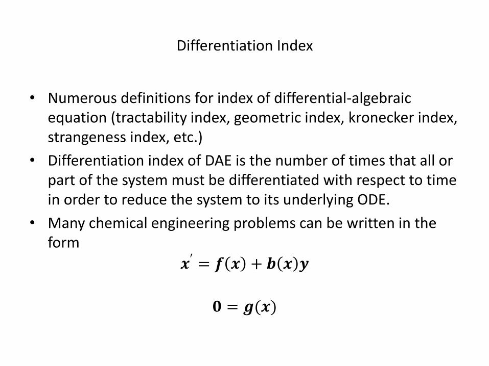
Differentiation Index
• Numerous definitions for index of differential-algebraic equation (tractability index, geometric index, kronecker index, strangeness index, etc.)
• Differentiation index of DAE is the number of times that all or part of the system must be differentiated with respect to time in order to reduce the system to its underlying ODE.
• Many chemical engineering problems can be written in the form
𝒙′ = 𝒇 𝒙 + 𝒃 𝒙 𝒚
𝟎 = 𝒈(𝒙)
Differentiation Index
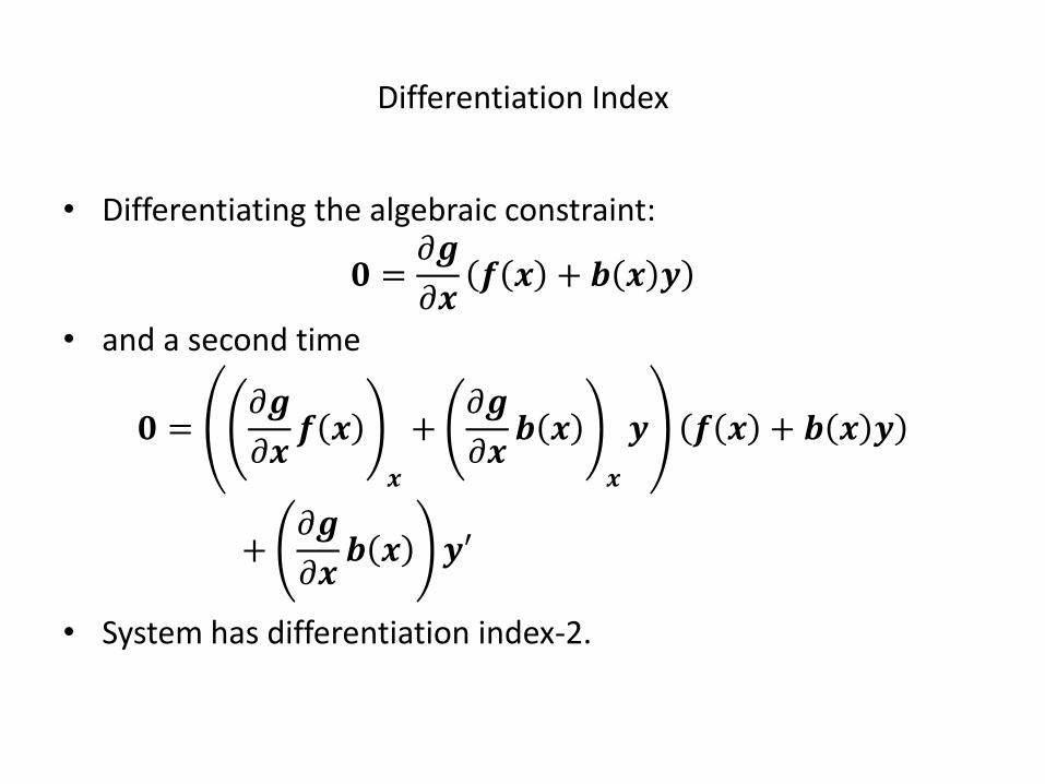
• Differentiating the algebraic constraint:
𝟎 =𝜕𝒈
𝜕𝒙𝒇 𝒙 + 𝒃 𝒙 𝒚
• and a second time
𝟎 =𝜕𝒈
𝜕𝒙𝒇 𝒙
𝒙
+𝜕𝒈
𝜕𝒙𝒃 𝒙
𝒙
𝒚 𝒇 𝒙 + 𝒃 𝒙 𝒚
+𝜕𝒈
𝜕𝒙𝒃 𝒙 𝒚′
• System has differentiation index-2.
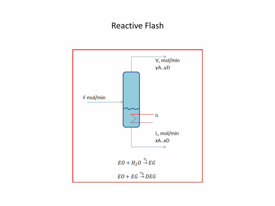
Reactive Flash
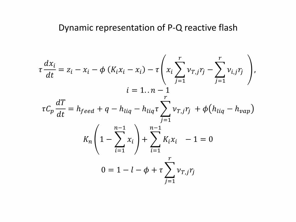
Dynamic representation of P-Q reactive flash
𝜏𝑑𝑥𝑖𝑑𝑡= 𝑧𝑖 − 𝑥𝑖 − 𝜙 𝐾𝑖𝑥𝑖 − 𝑥𝑖 − 𝜏 𝑥𝑖 𝜈𝑇,𝑗𝑟𝑗 −
𝑟
𝑗=1
𝜈𝑖,𝑗𝑟𝑗
𝑟
𝑗=1
,
𝑖 = 1. . 𝑛 − 1
𝜏𝐶𝑝𝑑𝑇
𝑑𝑡= ℎ𝑓𝑒𝑒𝑑 + 𝑞 − ℎ𝑙𝑖𝑞 − ℎ𝑙𝑖𝑞𝜏 𝜈𝑇,𝑗𝑟𝑗
𝑟
𝑗=1
+ 𝜙 ℎ𝑙𝑖𝑞 − ℎ𝑣𝑎𝑝
𝐾𝑛 1 − 𝑥𝑖
𝑛−1
𝑖=1
+ 𝐾𝑖𝑥𝑖
𝑛−1
𝑖=1
− 1 = 0
0 = 1 − 𝑙 − 𝜙 + 𝜏 𝜈𝑇,𝑗𝑟𝑗
𝑟
𝑗=1
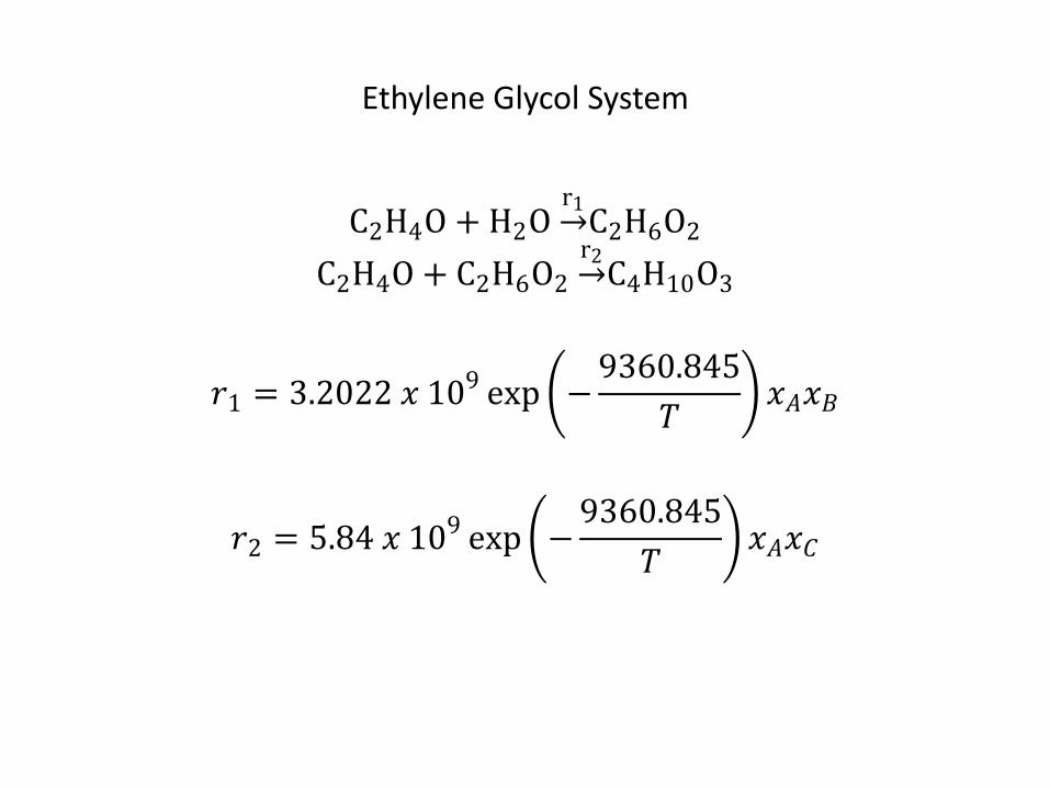
Ethylene Glycol System
C2H4O + H2O r1 C2H6O2
C2H4O + C2H6O2 r2 C4H10O3
𝑟1 = 3.2022 𝑥 109 exp −
9360.845
𝑇𝑥𝐴𝑥𝐵
𝑟2 = 5.84 𝑥 109 exp −
9360.845
𝑇𝑥𝐴𝑥𝐶
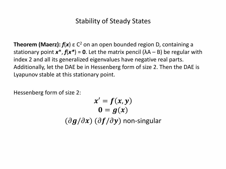
Stability of Steady States
Theorem (Maerz): f(x) ε C2 on an open bounded region D, containing a stationary point x*, f(x*) = 0. Let the matrix pencil (λA – B) be regular with index 2 and all its generalized eigenvalues have negative real parts. Additionally, let the DAE be in Hessenberg form of size 2. Then the DAE is Lyapunov stable at this stationary point.
Hessenberg form of size 2:
𝒙′ = 𝒇 𝒙, 𝒚 𝟎 = 𝒈(𝒙)
(𝜕𝒈/𝜕𝒙) (𝜕𝒇/𝜕𝒚) non-singular
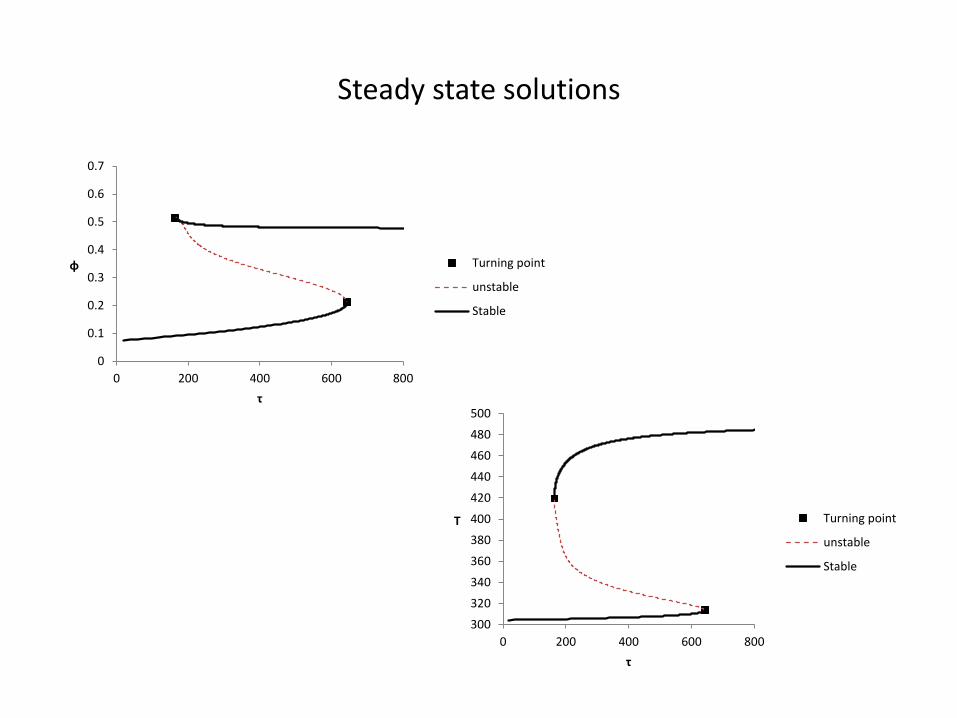
Steady state solutions
0
0.1
0.2
0.3
0.4
0.5
0.6
0.7
0 200 400 600 800
φ
τ
Turning point
unstable
Stable
300
320
340
360
380
400
420
440
460
480
500
0 200 400 600 800
T
τ
Turning point
unstable
Stable
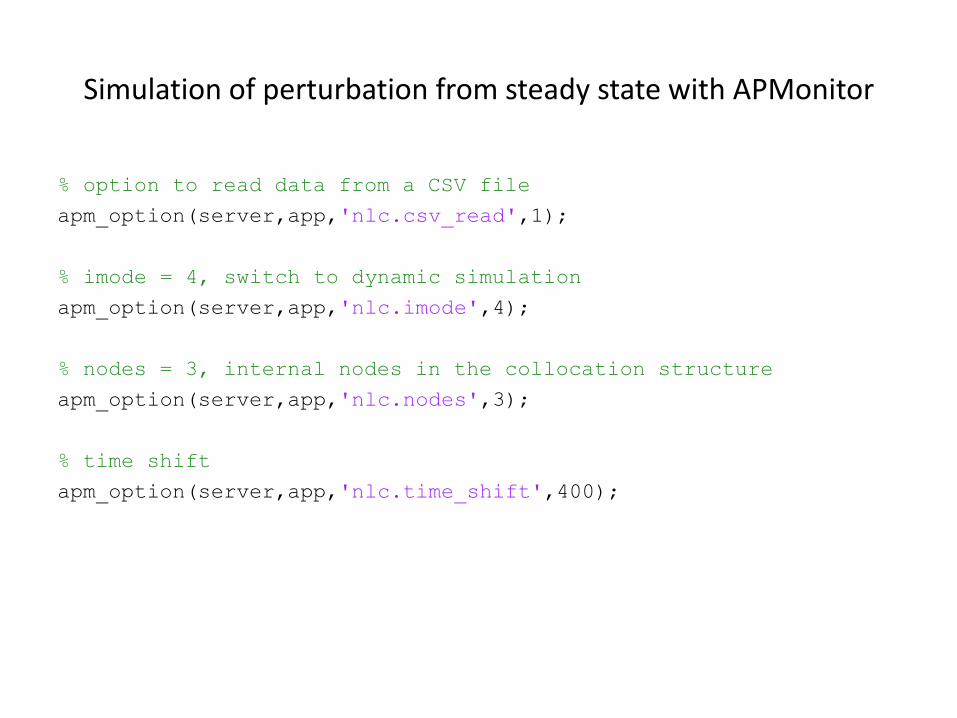
Simulation of perturbation from steady state with APMonitor
% option to read data from a CSV file
apm_option(server,app,'nlc.csv_read',1);
% imode = 4, switch to dynamic simulation
apm_option(server,app,'nlc.imode',4);
% nodes = 3, internal nodes in the collocation structure
apm_option(server,app,'nlc.nodes',3);
% time shift
apm_option(server,app,'nlc.time_shift',400);
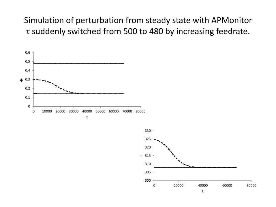
Simulation of perturbation from steady state with APMonitor τ suddenly switched from 500 to 480 by increasing feedrate.
0
0.1
0.2
0.3
0.4
0.5
0.6
0 10000 20000 30000 40000 50000 60000 70000 80000
φ
t
300
305
310
315
320
325
330
0 20000 40000 60000 80000
T
t

Simulation of perturbation from steady state with APMonitor τ suddenly switched from 500 to 501 by decreasing feedrate.
-0.4
-0.3
-0.2
-0.1
0
0.1
0.2
0.3
0.4
0.5
0.6
0 10000 20000 30000 40000 50000
t, min
300
320
340
360
380
400
420
440
460
480
500
0 10000 20000 30000 40000 50000
T, °
K
t, min
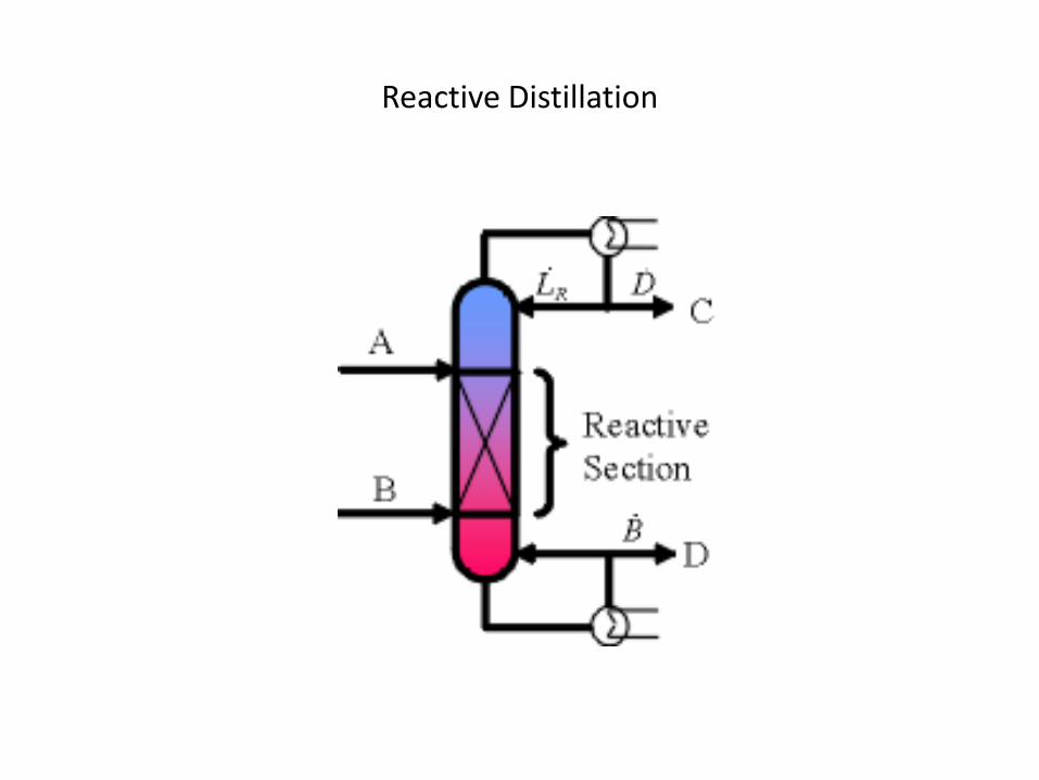
Reactive Distillation
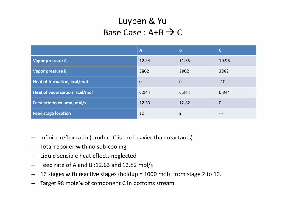
Luyben & Yu Base Case : A+B C
– Infinite reflux ratio (product C is the heavier than reactants)
– Total reboiler with no sub-cooling
– Liquid sensible heat effects neglected
– Feed rate of A and B :12.63 and 12.82 mol/s
– 16 stages with reactive stages (holdup = 1000 mol) from stage 2 to 10.
– Target 98 mole% of component C in bottoms stream
A B C
Vapor pressure Aj 12.34 11.65 10.96
Vapor pressure Bj 3862 3862 3862
Heat of formation, kcal/mol 0 0 -10
Heat of vaporization, kcal/mol 6.944 6.944 6.944
Feed rate to column, mol/s 12.63 12.82 0
Feed stage location 10 2 ---
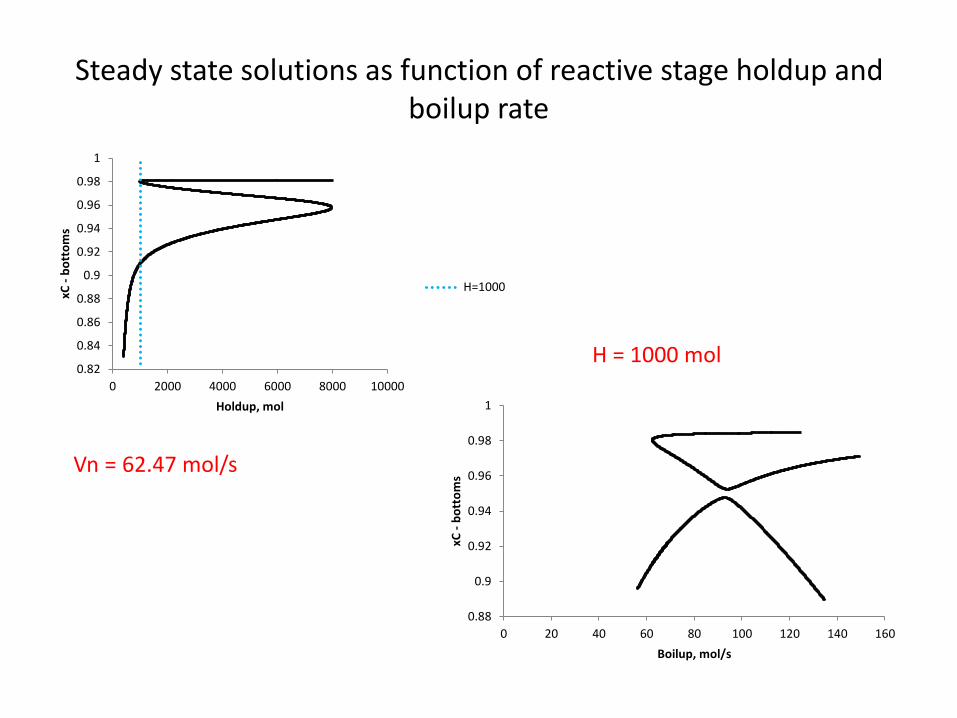
Steady state solutions as function of reactive stage holdup and boilup rate
0.82
0.84
0.86
0.88
0.9
0.92
0.94
0.96
0.98
1
0 2000 4000 6000 8000 10000
xC -
bo
tto
ms
Holdup, mol
H=1000
0.88
0.9
0.92
0.94
0.96
0.98
1
0 20 40 60 80 100 120 140 160
xC -
bo
tto
ms
Boilup, mol/s
Vn = 62.47 mol/s
H = 1000 mol
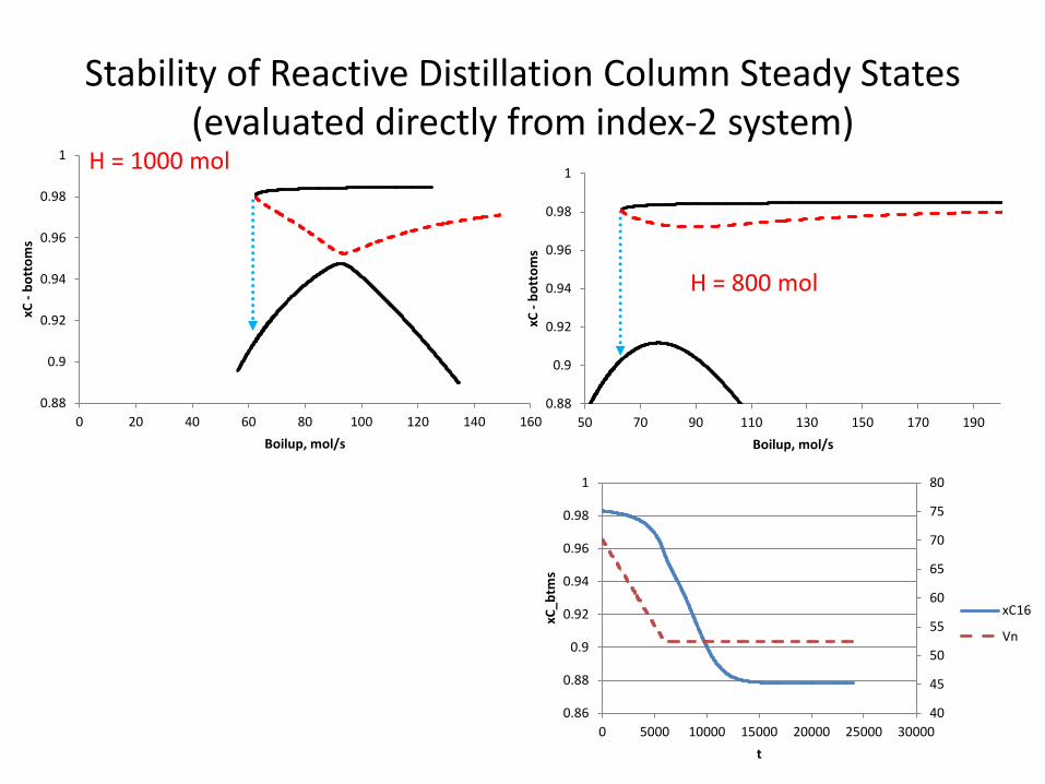
Stability of Reactive Distillation Column Steady States (evaluated directly from index-2 system)
0.88
0.9
0.92
0.94
0.96
0.98
1
0 20 40 60 80 100 120 140 160
xC -
bo
tto
ms
Boilup, mol/s
0.88
0.9
0.92
0.94
0.96
0.98
1
50 70 90 110 130 150 170 190
xC -
bo
tto
ms
Boilup, mol/s
H = 800 mol
H = 1000 mol
40
45
50
55
60
65
70
75
80
0.86
0.88
0.9
0.92
0.94
0.96
0.98
1
0 5000 10000 15000 20000 25000 30000
xC_b
tms
t
xC16
Vn
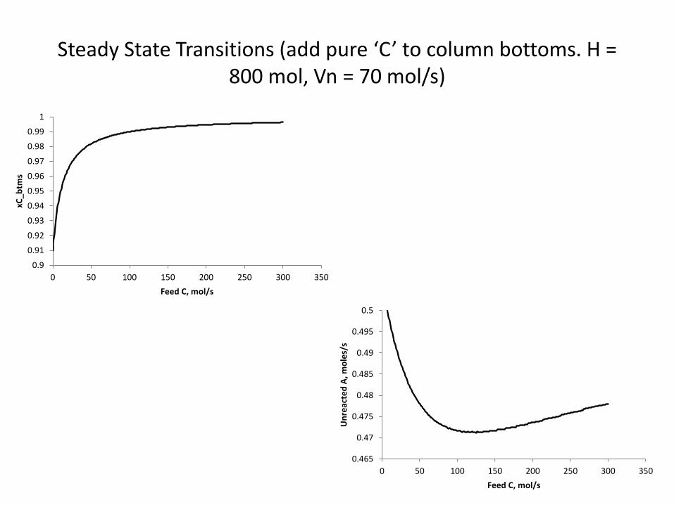
Steady State Transitions (add pure ‘C’ to column bottoms. H = 800 mol, Vn = 70 mol/s)
0.9
0.91
0.92
0.93
0.94
0.95
0.96
0.97
0.98
0.99
1
0 50 100 150 200 250 300 350
xC_b
tms
Feed C, mol/s
0.465
0.47
0.475
0.48
0.485
0.49
0.495
0.5
0 50 100 150 200 250 300 350
Un
reac
ted
A, m
ole
s/s
Feed C, mol/s
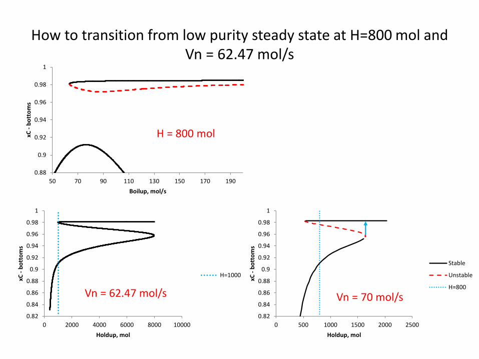
How to transition from low purity steady state at H=800 mol and Vn = 62.47 mol/s
Vn = 70 mol/s
0.82
0.84
0.86
0.88
0.9
0.92
0.94
0.96
0.98
1
0 500 1000 1500 2000 2500
xC -
bo
tto
ms
Holdup, mol
Stable
Unstable
H=800
0.82
0.84
0.86
0.88
0.9
0.92
0.94
0.96
0.98
1
0 2000 4000 6000 8000 10000
xC -
bo
tto
ms
Holdup, mol
H=1000
Vn = 62.47 mol/s
0.88
0.9
0.92
0.94
0.96
0.98
1
50 70 90 110 130 150 170 190
xC -
bo
tto
ms
Boilup, mol/s
H = 800 mol
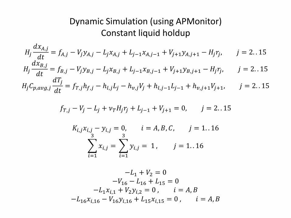
Dynamic Simulation (using APMonitor) Constant liquid holdup
𝐻𝑗𝑑𝑥𝐴,𝑗
𝑑𝑡= 𝑓𝐴,𝑗 − 𝑉𝑗𝑦𝐴,𝑗 − 𝐿𝑗𝑥𝐴,𝑗 + 𝐿𝑗−1𝑥𝐴,𝑗−1 + 𝑉𝑗+1𝑦𝐴,𝑗+1 − 𝐻𝑗𝑟𝑗 , 𝑗 = 2. . 15
𝐻𝑗𝑑𝑥𝐵,𝑗
𝑑𝑡= 𝑓𝐵,𝑗 − 𝑉𝑗𝑦𝐵,𝑗 − 𝐿𝑗𝑥𝐵,𝑗 + 𝐿𝑗−1𝑥𝐵,𝑗−1 + 𝑉𝑗+1𝑦𝐵,𝑗+1 − 𝐻𝑗𝑟𝑗 , 𝑗 = 2. . 15
𝐻𝑗𝐶𝑝,𝑎𝑣𝑔,𝑗𝑑𝑇𝑗
𝑑𝑡= 𝑓𝑇,𝑗ℎ𝑓,𝑗 − ℎ𝑙,𝑗𝐿𝑗 − ℎ𝑣,𝑗𝑉𝑗 + ℎ𝑙,𝑗−1𝐿𝑗−1 + ℎ𝑣,𝑗+1𝑉𝑗+1, 𝑗 = 2. . 15
𝑓𝑇,𝑗 − 𝑉𝑗 − 𝐿𝑗 + 𝜈𝑇𝐻𝑗𝑟𝑗 + 𝐿𝑗−1 + 𝑉𝑗+1 = 0, 𝑗 = 2. . 15
𝐾𝑖,𝑗𝑥𝑖,𝑗 − 𝑦𝑖,𝑗 = 0, 𝑖 = 𝐴, 𝐵, 𝐶, 𝑗 = 1. . 16
𝑥𝑖,𝑗 =
3
𝑖=1
𝑦𝑖,𝑗 = 1
3
𝑖=1
, 𝑗 = 1. . 16
−𝐿1 + 𝑉2 = 0
−𝑉16 − 𝐿16 + 𝐿15 = 0 −𝐿1𝑥𝑖,1 + 𝑉2𝑦𝑖,2 = 0 , 𝑖 = 𝐴, 𝐵
−𝐿16𝑥𝑖,16 − 𝑉16𝑦𝑖,16 + 𝐿15𝑥𝑖,15 = 0 , 𝑖 = 𝐴, 𝐵
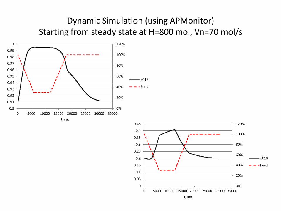
Dynamic Simulation (using APMonitor) Starting from steady state at H=800 mol, Vn=70 mol/s
0%
20%
40%
60%
80%
100%
120%
0.9
0.91
0.92
0.93
0.94
0.95
0.96
0.97
0.98
0.99
1
0 5000 10000 15000 20000 25000 30000 35000
t, sec
xC16
Feed
0%
20%
40%
60%
80%
100%
120%
0
0.05
0.1
0.15
0.2
0.25
0.3
0.35
0.4
0.45
0 5000 10000 15000 20000 25000 30000 35000
t, sec
xC10
Feed
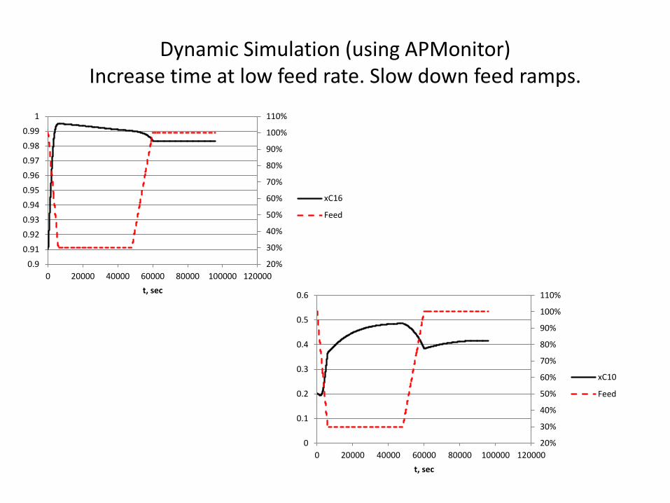
Dynamic Simulation (using APMonitor) Increase time at low feed rate. Slow down feed ramps.
20%
30%
40%
50%
60%
70%
80%
90%
100%
110%
0.9
0.91
0.92
0.93
0.94
0.95
0.96
0.97
0.98
0.99
1
0 20000 40000 60000 80000 100000 120000
t, sec
xC16
Feed
20%
30%
40%
50%
60%
70%
80%
90%
100%
110%
0
0.1
0.2
0.3
0.4
0.5
0.6
0 20000 40000 60000 80000 100000 120000
t, sec
xC10
Feed
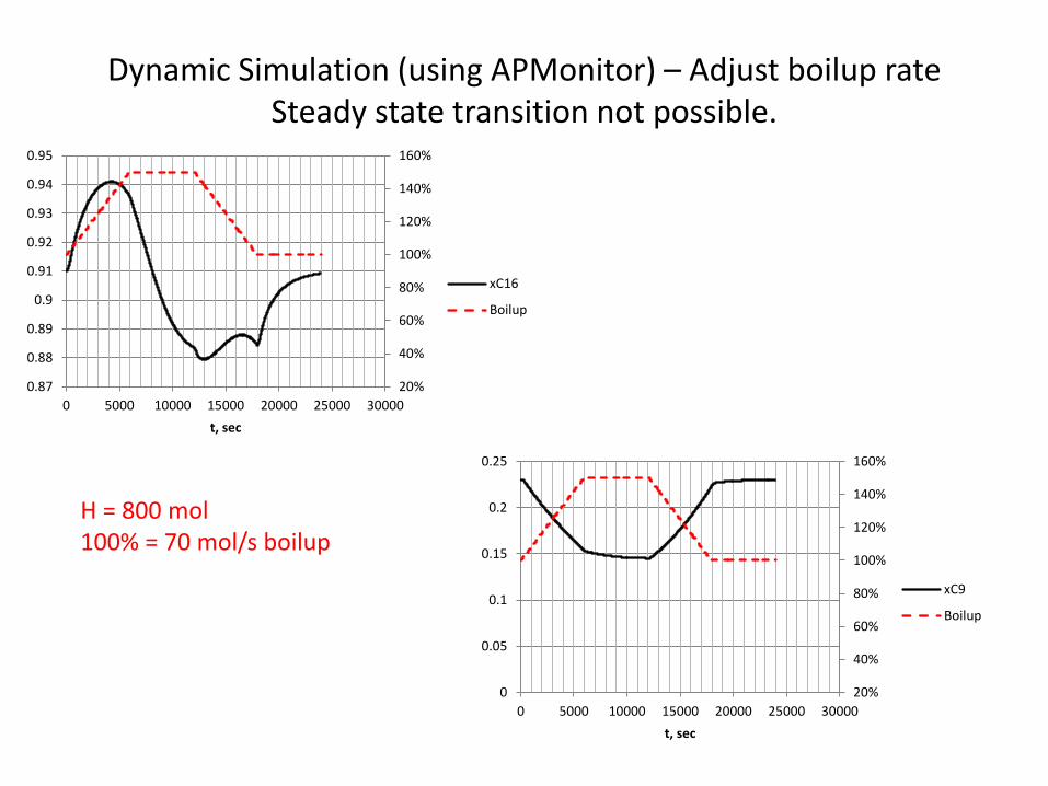
Dynamic Simulation (using APMonitor) – Adjust boilup rate Steady state transition not possible.
H = 800 mol 100% = 70 mol/s boilup
20%
40%
60%
80%
100%
120%
140%
160%
0
0.05
0.1
0.15
0.2
0.25
0 5000 10000 15000 20000 25000 30000
t, sec
xC9
Boilup
20%
40%
60%
80%
100%
120%
140%
160%
0.87
0.88
0.89
0.9
0.91
0.92
0.93
0.94
0.95
0 5000 10000 15000 20000 25000 30000
t, sec
xC16
Boilup

Dynamic Simulation – Introduce Holdup as dynamic variable
𝑑 𝐻𝑗𝑥𝐴,𝑗
𝑑𝑡= 𝑓𝐴,𝑗− 𝑉𝑗𝑦𝐴,𝑗 − 𝐿𝑗𝑥𝐴,𝑗 + 𝐿𝑗−1𝑥𝐴,𝑗−1 + 𝑉𝑗+1𝑦𝐴,𝑗+1 −𝐻𝑗𝑟𝑗, 𝑗 = 2. . 15
𝑑 𝐻𝑗𝑥𝐵,𝑗
𝑑𝑡= 𝑓𝐵,𝑗− 𝑉𝑗𝑦𝐵,𝑗 − 𝐿𝑗𝑥𝐵,𝑗 + 𝐿𝑗−1𝑥𝐵,𝑗−1 + 𝑉𝑗+1𝑦𝐵,𝑗+1 − 𝐻𝑗𝑟𝑗, 𝑗 = 2. . 15
𝐶𝑝,𝑎𝑣𝑔,𝑗𝑑 𝐻𝑗 𝑇𝑗 − 𝑇0
𝑑𝑡= 𝑓𝑇,𝑗ℎ𝑓,𝑗 − ℎ𝑙,𝑗𝐿𝑗 − ℎ𝑣,𝑗𝑉𝑗 + ℎ𝑙,𝑗−1𝐿𝑗−1 + ℎ𝑣,𝑗+1𝑉𝑗+1, 𝑗 = 2. . 15
𝑑𝐻𝑗
𝑑𝑡= 𝑓𝑇,𝑗− 𝑉𝑗 − 𝐿𝑗 + 𝜈𝑇𝐻𝑗𝑟𝑗 + 𝐿𝑗−1 + 𝑉𝑗+1, 𝑗 = 2. . 15
𝐾𝑖,𝑗𝑥𝑖,𝑗 − 𝑦𝑖,𝑗 = 0, 𝑖 = 𝐴, 𝐵, 𝐶, 𝑗 = 1. . 16
𝑥𝑖,𝑗 =
3
𝑖=1
𝑦𝑖,𝑗 = 1
3
𝑖=1
, 𝑗 = 1. . 16
−𝐿1 + 𝑉2 = 0
−𝑉16 − 𝐿16 + 𝐿15 = 0 −𝐿1𝑥𝑖,1 + 𝑉2𝑦𝑖,2 = 0 , 𝑖 = 𝐴, 𝐵
−𝐿16𝑥𝑖,16 − 𝑉16𝑦𝑖,16 + 𝐿15𝑥𝑖,15 = 0 , 𝑖 = 𝐴, 𝐵
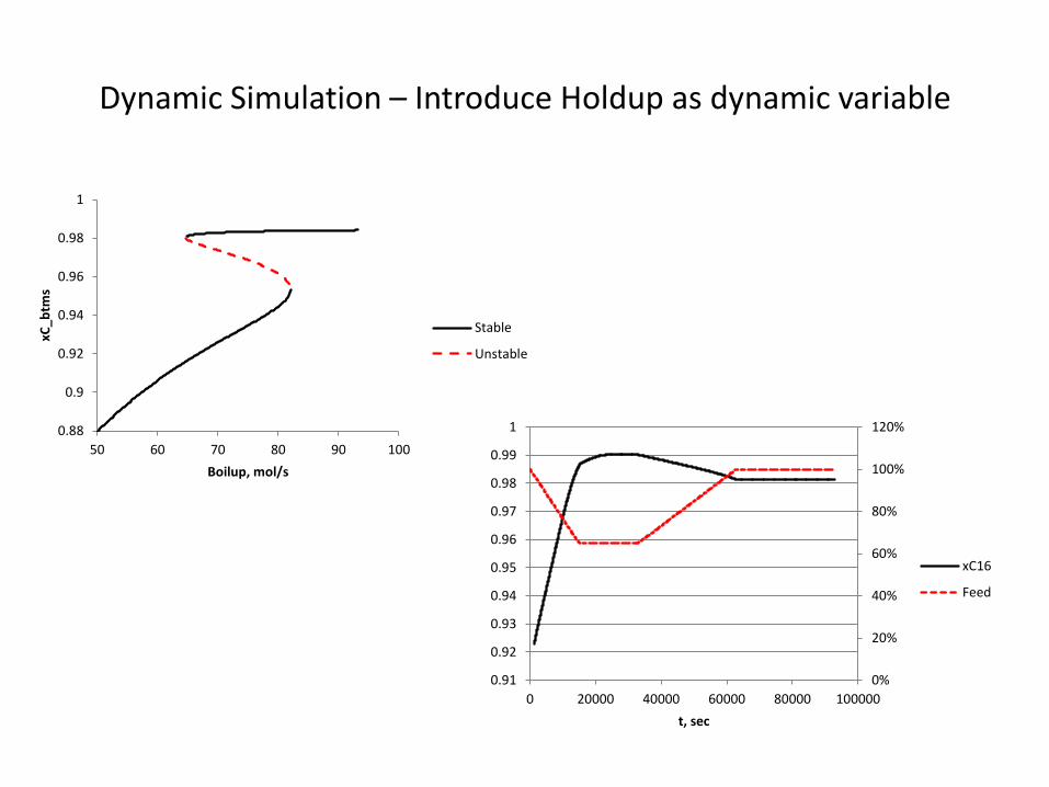
Dynamic Simulation – Introduce Holdup as dynamic variable
0.88
0.9
0.92
0.94
0.96
0.98
1
50 60 70 80 90 100
xC_b
tms
Boilup, mol/s
Stable
Unstable
0%
20%
40%
60%
80%
100%
120%
0.91
0.92
0.93
0.94
0.95
0.96
0.97
0.98
0.99
1
0 20000 40000 60000 80000 100000
t, sec
xC16
Feed
Conclusions
• Differential algebraic systems defining reactive flash and reactive distillation systems were in Hessenberg form of size 2.
• Stability of steady states can be calculated at each point on the bifurcation path.
• APMonitor can reliably traverse the orbit of these index-2 DAE IVP.
• Index reductions such as that proposed by Kumar et al. (2009) (Comput. Chem. Engng., 33, p. 1336) to solve for intermediate vapor flows not required.
• Theses dynamic simulations are a powerful tool for checking viability of various steady state transitions.


![Separation-like problems for regular languagesMarc Zeitoun[1.5ex]Joint work with Thomas Place Created Date 7/27/2016 1:34:44 PM](https://img.pdfslide.tips/doc/110x75/5f29df98d60a006b091e6f76/separation-like-problems-for-regular-languages-marc-zeitoun15exjoint-work-with.jpg)