Study of an antenna array for direction finding

= = Master Thesis Project = =

William Eriksson Selin

Study of antenna array for direction finding

Master´s Thesis in Engineering Physics, 30 Credits [5FY123]

Proant AB

Department of Physics, Umeå University, Sweden

Author: William Eriksson Selin - wier0004 (wier0004@student.umu.se)

Supervisors: Viktor Lundström (viktor.lundstrom@proantantennas.com),Daniel Nilsson (daniel.pg.nilsson@umu.se)

Examiner: Herbert Gunell (herbert@herbertgunell.se)

i

Acknowledgments

Proant AB has given me the opportunity to do a project in an interesting topic and have providedme with an inspiring work environment that have allowed me to gain a lot of new knowledgeabout antenna development and antennas in general. For this I want to thank Tomas, Anttiand Ingela and a special thanks to my supervisor at Proant AB Viktor Lundström for beinga high energy person throughout the project. I want to thank Umeå University for providinga high quality education in Engineering Physics and my examiner at Umeå University HerbertGunell. I want to thank my student colleague David Chaoran Chen Bataski for all the goodadvice throughout my education. And thank you to my girlfriend Emmy Sjöström and everyoneelse in my family for all the love and support.

ii

Dedicated to Mio, my son.

iii

Abstract

The new Bluetooth standard (Bluetooth 5.1) contains direction finding specifications. Specifica-tions for received signal strength indicator(RSSI) using measures of signal strength in order togive a sense of how far away an object is has been present in earlier versions. It will now be ac-companied with the possibility of angle of arrival estimation(AoA). AoA estimation in Bluetoothutilizes antenna arrays. Antenna arrays are formations of many individual antenna elementsworking together. The difference between the measured data at each antenna is dependent onthe orientation and position of the antenna elements as well as on phase of an incoming elec-tromagnetic signal. By looking at the phase shifts between the antenna elements in an antennaarray it is possible to find an estimation of the direction of where the incoming signal is comingfrom.

The goal of this thesis is to investigate if the NicheTM antenna(concept developed by Proant AB)is applicable for AoA estimation. In the project we have simulated the different characteristics ofthe Niche antenna and done extensive simulations of different types of configurations of an Nicheantenna array. The commercial electromagnetics simulator CST MW studio suite has been usedfor simulations. A formation that works well with regards to stability and mutual coupling hasbeen found. The simulated results have also been confirmed by measurements on a mechanicallyconstructed antenna array. Measurements have been carried out in an anechoic chamber. Wehave done full radiation pattern measurements of the antenna array. The antenna array that wehave created can estimate the angle of arrival of an incoming signal with an accuracy of ±2.7

with a certainty of one standard deviation. For increased accuracy in the AoA estimation aMATLAB code utilizing the MUSIC(MUltiple SIgnal Classification) algorithm with our variantof the steering vector has been written.

Contents

1 Introduction 11.1 The Niche concept . . . . . . . . . . . . . . . . . . . . . . . . . . . . . . . . . . . 21.2 Bluetooth 5.1 . . . . . . . . . . . . . . . . . . . . . . . . . . . . . . . . . . . . . . 51.3 Angle of arrival . . . . . . . . . . . . . . . . . . . . . . . . . . . . . . . . . . . . . 6

2 Theory 72.1 Electromagnetic radiation . . . . . . . . . . . . . . . . . . . . . . . . . . . . . . . 72.2 Antenna introduction . . . . . . . . . . . . . . . . . . . . . . . . . . . . . . . . . 72.3 The basic principle of AoA . . . . . . . . . . . . . . . . . . . . . . . . . . . . . . 82.4 Antenna array design considerations . . . . . . . . . . . . . . . . . . . . . . . . . 11

3 Method 123.1 Simulation procedure . . . . . . . . . . . . . . . . . . . . . . . . . . . . . . . . . . 12

3.1.1 Niche antenna characteristics . . . . . . . . . . . . . . . . . . . . . . . . . 123.2 Calculation of the expected phase value . . . . . . . . . . . . . . . . . . . . . . . 143.3 Measurement procedure . . . . . . . . . . . . . . . . . . . . . . . . . . . . . . . . 14

3.3.1 Anechoic chamber . . . . . . . . . . . . . . . . . . . . . . . . . . . . . . . 143.3.2 Realization of the antenna array prototype . . . . . . . . . . . . . . . . . 163.3.3 Antenna array prototype under testing . . . . . . . . . . . . . . . . . . . . 173.3.4 Cable switch . . . . . . . . . . . . . . . . . . . . . . . . . . . . . . . . . . 19

3.4 Post processing and the AoA Algorithm . . . . . . . . . . . . . . . . . . . . . . . 20

4 Results 214.1 Antenna array configuration . . . . . . . . . . . . . . . . . . . . . . . . . . . . . . 214.2 Antenna array phase simulation . . . . . . . . . . . . . . . . . . . . . . . . . . . . 214.3 Antenna array measurements . . . . . . . . . . . . . . . . . . . . . . . . . . . . . 21

5 Discussion 295.1 Future Development . . . . . . . . . . . . . . . . . . . . . . . . . . . . . . . . . . 30

6 References 32

A Appendix iA.1 Pseudo code . . . . . . . . . . . . . . . . . . . . . . . . . . . . . . . . . . . . . . . iA.2 IQ sampling . . . . . . . . . . . . . . . . . . . . . . . . . . . . . . . . . . . . . . . iA.3 Bluetooth 5.1 . . . . . . . . . . . . . . . . . . . . . . . . . . . . . . . . . . . . . . iiA.4 The coupling matrix . . . . . . . . . . . . . . . . . . . . . . . . . . . . . . . . . . iiA.5 Models in CST . . . . . . . . . . . . . . . . . . . . . . . . . . . . . . . . . . . . . iiiA.6 Simulation results . . . . . . . . . . . . . . . . . . . . . . . . . . . . . . . . . . . iii

i

1 Introduction

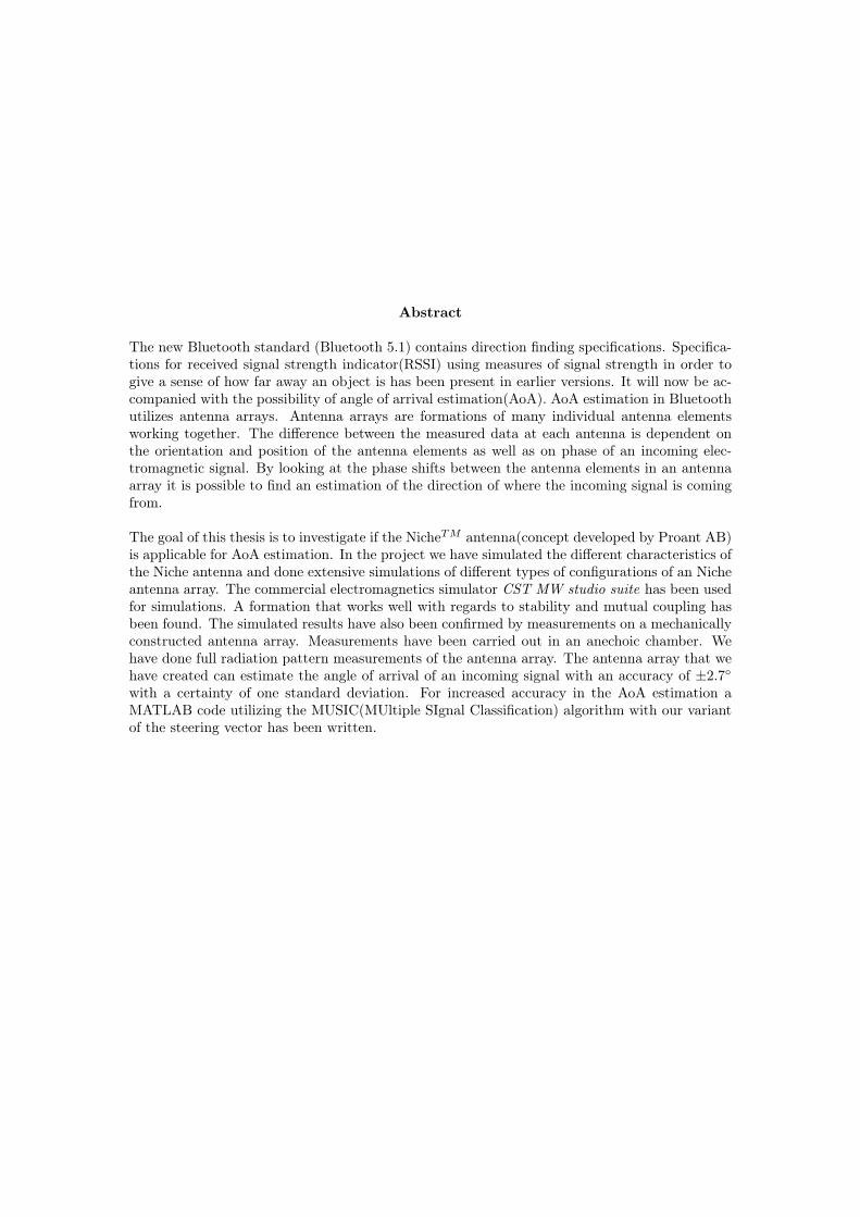
A technology allowing for high precision indoor positioning is on the rise to be available to themasses[1]. Direction finding is more on the topic than ever with cheaper antennas, smaller an-tennas, smarter designs and pushed forward by the new Bluetooth standard(Bluetooth 5.1). Thestandard contains specifications for how direction finding should be done in Bluetooth devices. Itutilizes antenna arrays which is a formation of many antenna elements[2]. The measured data ateach antenna element together with information about the element orientation and the specificformation of the antenna array can be used for angle of arrival(AoA) estimations. Estimatingangles of incoming electromagnetic signals is done by measuring the phase of said signal. Thesignals phase shift between two consecutive antennas together with the distance between themwill be able to give you the AoA as long as you know the wavelength. The wavelength is knownwhen working with specific frequencies. In AoA estimation the signal from a transmitting tag issent out. The transmitted signal arrives at the antenna array and the phase at each antenna ele-ment is measured with the aid of a RF-switch and the measured signal is collected by a receiver.For increased accuracy over direct measurements of the phase an AoA algorithm does the finalstep of estimating the angle of arrival of the signal. A graphical description of the AoA workflowspecified by Bluetooth 5.1 is shown in figure 1. In this project we have written a code for the

Figure 1 – Figure describing the AoA workflow in Bluetooth 5.1. Image source: BluetoothSIG(special interest group)[3].

AoA estimation utilizing the MUSIC(MUltiple SIgnal Classification) algorithm. The algorithmis subspace subspace based which means that is exploits the noise eigenvector subspace[4], whichbasically means that the eigenvalues of the noise and the signal are separated. The eigenvectorsof the noise are always perpendicular to the angle of arrival and it is this property that is used inthe MUSIC algorithm. In order to give information about the antenna array a so called steeringvector is used. The steering vector contains information about the orientation of the individualantenna elements as well as the formation of the antenna array(see Eq. 5 in section 2). The codeis written in MATLAB with our own version of the steering vector. This takes the measuredphase shifts directly, computes the eigendecomposition and estimates the angle of arrival usingthe eigenvalues of the noise between the antenna elements. The commercial electromagneticssimulator CST studio suite has been used to determine the characteristics of the Niche antennaand to do phase measurements of the antenna array with a plane wave excitation. CST standsfor Computer Simulation Technology and is an electromagnetics simulation software. MATLABhas been used for data managing and visualization of data. In this project we have investigatedthe Niche antenna and how different constellations of the antenna array are affecting the mutual

1

coupling between antenna elements. Mutual coupling refers to the unintended communicationbetween antenna elements and is in general something that should be on a low level in antennaarrays. The main goal of this thesis is to investigate if the NicheTM antenna(concept developedby Proant AB) is applicable for AoA estimation.

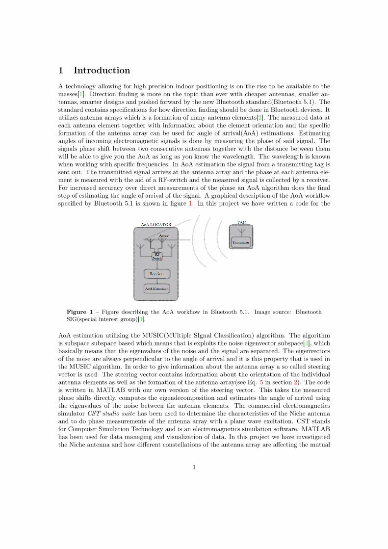
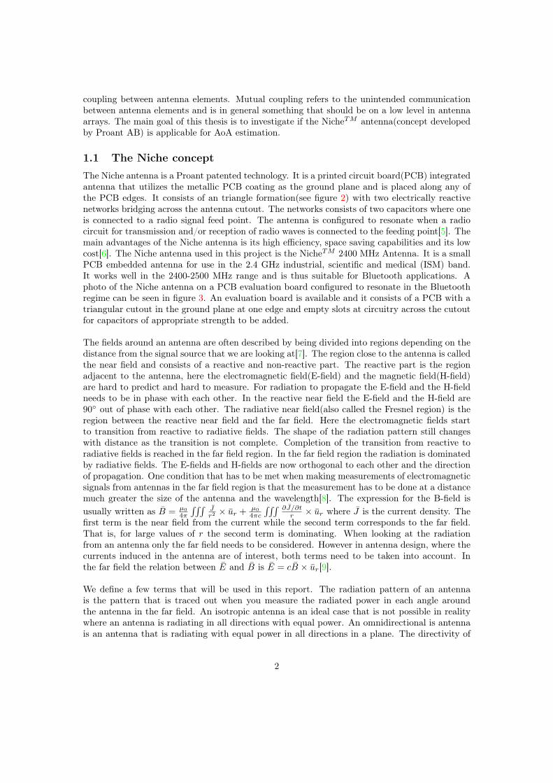
1.1 The Niche conceptThe Niche antenna is a Proant patented technology. It is a printed circuit board(PCB) integratedantenna that utilizes the metallic PCB coating as the ground plane and is placed along any ofthe PCB edges. It consists of an triangle formation(see figure 2) with two electrically reactivenetworks bridging across the antenna cutout. The networks consists of two capacitors where oneis connected to a radio signal feed point. The antenna is configured to resonate when a radiocircuit for transmission and/or reception of radio waves is connected to the feeding point[5]. Themain advantages of the Niche antenna is its high efficiency, space saving capabilities and its lowcost[6]. The Niche antenna used in this project is the NicheTM 2400 MHz Antenna. It is a smallPCB embedded antenna for use in the 2.4 GHz industrial, scientific and medical (ISM) band.It works well in the 2400-2500 MHz range and is thus suitable for Bluetooth applications. Aphoto of the Niche antenna on a PCB evaluation board configured to resonate in the Bluetoothregime can be seen in figure 3. An evaluation board is available and it consists of a PCB with atriangular cutout in the ground plane at one edge and empty slots at circuitry across the cutoutfor capacitors of appropriate strength to be added.

The fields around an antenna are often described by being divided into regions depending on thedistance from the signal source that we are looking at[7]. The region close to the antenna is calledthe near field and consists of a reactive and non-reactive part. The reactive part is the regionadjacent to the antenna, here the electromagnetic field(E-field) and the magnetic field(H-field)are hard to predict and hard to measure. For radiation to propagate the E-field and the H-fieldneeds to be in phase with each other. In the reactive near field the E-field and the H-field are90 out of phase with each other. The radiative near field(also called the Fresnel region) is theregion between the reactive near field and the far field. Here the electromagnetic fields startto transition from reactive to radiative fields. The shape of the radiation pattern still changeswith distance as the transition is not complete. Completion of the transition from reactive toradiative fields is reached in the far field region. In the far field region the radiation is dominatedby radiative fields. The E-fields and H-fields are now orthogonal to each other and the directionof propagation. One condition that has to be met when making measurements of electromagneticsignals from antennas in the far field region is that the measurement has to be done at a distancemuch greater the size of the antenna and the wavelength[8]. The expression for the B-field isusually written as B = µ0

4π

∫∫∫Jr2 × ur + µ0

4πc

∫∫∫ ∂J/∂tr × ur where J is the current density. The

first term is the near field from the current while the second term corresponds to the far field.That is, for large values of r the second term is dominating. When looking at the radiationfrom an antenna only the far field needs to be considered. However in antenna design, where thecurrents induced in the antenna are of interest, both terms need to be taken into account. Inthe far field the relation between E and B is E = cB × ur[9].

We define a few terms that will be used in this report. The radiation pattern of an antennais the pattern that is traced out when you measure the radiated power in each angle aroundthe antenna in the far field. An isotropic antenna is an ideal case that is not possible in realitywhere an antenna is radiating in all directions with equal power. An omnidirectional is antennais an antenna that is radiating with equal power in all directions in a plane. The directivity of

2

an antenna is a measure of how directional the radiation pattern is in relation to the isotropiccase(where the directivity is 0dB). The directivity of an antenna is defined as the maximumvalue of the radiation pattern(which is 1), divided by the average power in all directions. Thepeak gain of an antenna is a term that describes the amount of power radiated in the directionof peak radiation in comparison to the power radiated in the same direction but in the isotropiccase. Antenna gain is often used because it takes losses into account while directivity do not.If you know where a signal is coming from it is advantageous to have an antenna with as highgain as possible in that direction. Otherwise an antenna with low gain that is less directional isadvantageous so that the antenna will be able to get a reasonable gain in all directions neededin the application. The radiation pattern of the Niche antenna can be seen in figure 4. Anillustration to clarify in 3D how the axes are aligned in the figures showing radiation patternscan be seen in figure 5.

Figure 2 – A graphical description of an example of the Niche antenna on a PCB. Here designedto operate in the Bluetooth regime(2400-2483.5GHz). The yellow regions has a thin layer of coppermaterial placed on top of FR-4 which is a glass-reinforced epoxy laminate material(a dielectric).The yellow ground plane on the PCB and the yellow networks across the cutout are connected.The capacitors are marked in blue while the feeding network is marked in red.

Figure 3 – The Niche antenna on a PCB evaluation board configured to resonate in the Bluetoothregime(2400-2485MHz). The reactive components are marked out and consists of a mid and topcapacitance as well as the feeding point. In the evaluation board it is possible to connect twocapacitors in a row. The white line on the PCB marks out the cutout in the ground plane. Imagesource: Proant AB[6].

3

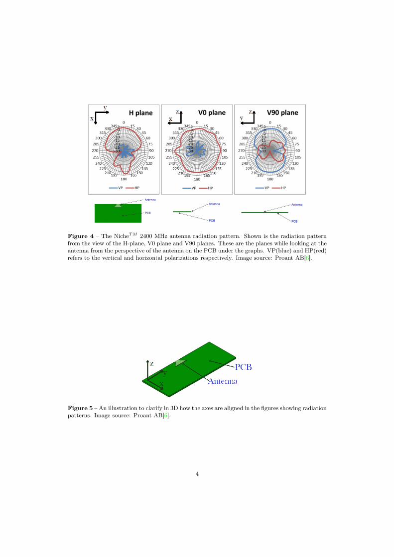
Figure 4 – The NicheTM 2400 MHz antenna radiation pattern. Shown is the radiation patternfrom the view of the H-plane, V0 plane and V90 planes. These are the planes while looking at theantenna from the perspective of the antenna on the PCB under the graphs. VP(blue) and HP(red)refers to the vertical and horizontal polarizations respectively. Image source: Proant AB[6].

Figure 5 – An illustration to clarify in 3D how the axes are aligned in the figures showing radiationpatterns. Image source: Proant AB[6].

4

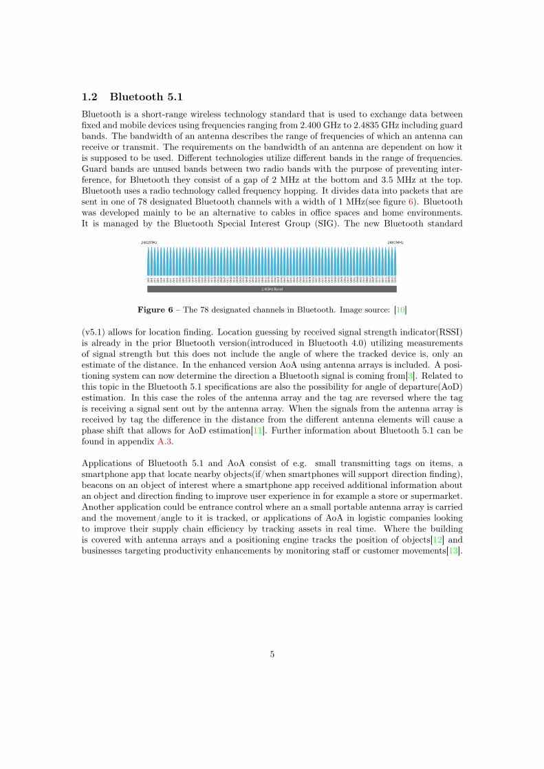
1.2 Bluetooth 5.1Bluetooth is a short-range wireless technology standard that is used to exchange data betweenfixed and mobile devices using frequencies ranging from 2.400 GHz to 2.4835 GHz including guardbands. The bandwidth of an antenna describes the range of frequencies of which an antenna canreceive or transmit. The requirements on the bandwidth of an antenna are dependent on how itis supposed to be used. Different technologies utilize different bands in the range of frequencies.Guard bands are unused bands between two radio bands with the purpose of preventing inter-ference, for Bluetooth they consist of a gap of 2 MHz at the bottom and 3.5 MHz at the top.Bluetooth uses a radio technology called frequency hopping. It divides data into packets that aresent in one of 78 designated Bluetooth channels with a width of 1 MHz(see figure 6). Bluetoothwas developed mainly to be an alternative to cables in office spaces and home environments.It is managed by the Bluetooth Special Interest Group (SIG). The new Bluetooth standard

Figure 6 – The 78 designated channels in Bluetooth. Image source: [10]

(v5.1) allows for location finding. Location guessing by received signal strength indicator(RSSI)is already in the prior Bluetooth version(introduced in Bluetooth 4.0) utilizing measurementsof signal strength but this does not include the angle of where the tracked device is, only anestimate of the distance. In the enhanced version AoA using antenna arrays is included. A posi-tioning system can now determine the direction a Bluetooth signal is coming from[3]. Related tothis topic in the Bluetooth 5.1 specifications are also the possibility for angle of departure(AoD)estimation. In this case the roles of the antenna array and the tag are reversed where the tagis receiving a signal sent out by the antenna array. When the signals from the antenna array isreceived by tag the difference in the distance from the different antenna elements will cause aphase shift that allows for AoD estimation[11]. Further information about Bluetooth 5.1 can befound in appendix A.3.

Applications of Bluetooth 5.1 and AoA consist of e.g. small transmitting tags on items, asmartphone app that locate nearby objects(if/when smartphones will support direction finding),beacons on an object of interest where a smartphone app received additional information aboutan object and direction finding to improve user experience in for example a store or supermarket.Another application could be entrance control where an a small portable antenna array is carriedand the movement/angle to it is tracked, or applications of AoA in logistic companies lookingto improve their supply chain efficiency by tracking assets in real time. Where the buildingis covered with antenna arrays and a positioning engine tracks the position of objects[12] andbusinesses targeting productivity enhancements by monitoring staff or customer movements[13].

5

1.3 Angle of arrivalAntenna arrays are used for two main purposes. Either to get a higher peak gain or to be able tosend or receive in a certain direction. Related to the latter is also the possibility of calculatingthe angle of arrival(AoA) of an incoming wave.

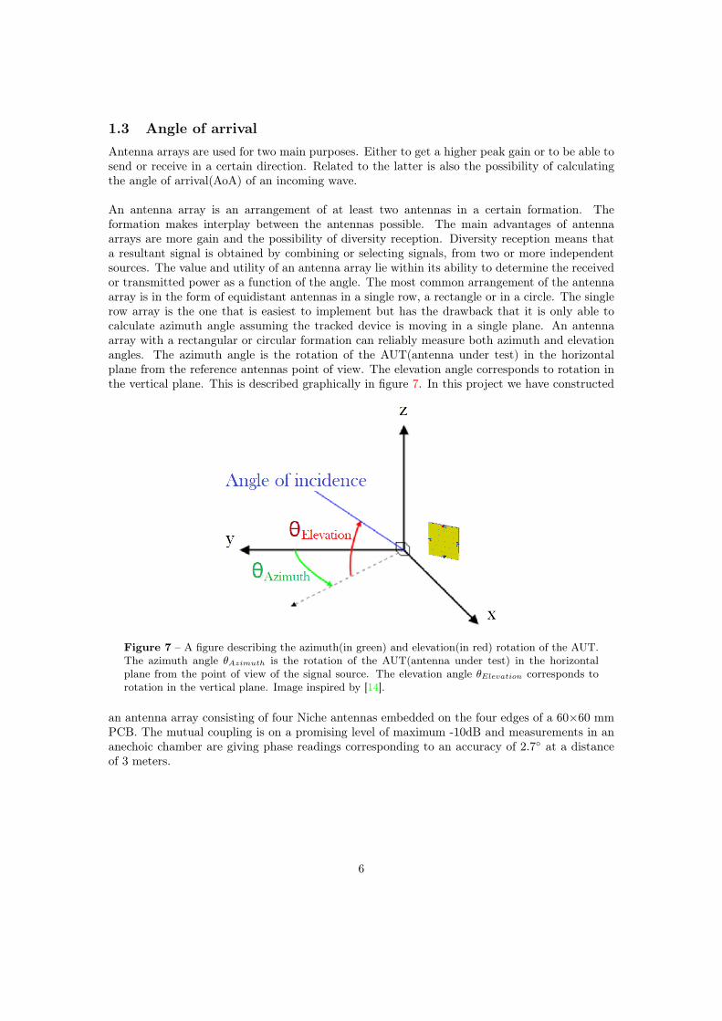
An antenna array is an arrangement of at least two antennas in a certain formation. Theformation makes interplay between the antennas possible. The main advantages of antennaarrays are more gain and the possibility of diversity reception. Diversity reception means thata resultant signal is obtained by combining or selecting signals, from two or more independentsources. The value and utility of an antenna array lie within its ability to determine the receivedor transmitted power as a function of the angle. The most common arrangement of the antennaarray is in the form of equidistant antennas in a single row, a rectangle or in a circle. The singlerow array is the one that is easiest to implement but has the drawback that it is only able tocalculate azimuth angle assuming the tracked device is moving in a single plane. An antennaarray with a rectangular or circular formation can reliably measure both azimuth and elevationangles. The azimuth angle is the rotation of the AUT(antenna under test) in the horizontalplane from the reference antennas point of view. The elevation angle corresponds to rotation inthe vertical plane. This is described graphically in figure 7. In this project we have constructed

Figure 7 – A figure describing the azimuth(in green) and elevation(in red) rotation of the AUT.The azimuth angle θAzimuth is the rotation of the AUT(antenna under test) in the horizontalplane from the point of view of the signal source. The elevation angle θElevation corresponds torotation in the vertical plane. Image inspired by [14].

an antenna array consisting of four Niche antennas embedded on the four edges of a 60×60 mmPCB. The mutual coupling is on a promising level of maximum -10dB and measurements in ananechoic chamber are giving phase readings corresponding to an accuracy of 2.7 at a distanceof 3 meters.

6

2 Theory

2.1 Electromagnetic radiationAn electromagnetic wave is a wave traveling through space consisting of an electric and a magneticfield that is perpendicular to each other and travels at the speed of light c. The fields oscillateswith a determinable frequency defined as its speed c divided by the wavelength λ that is thelength of the distance between two successive crests of the wave, that is to say f = c

λ .

2.2 Antenna introductionPolarization

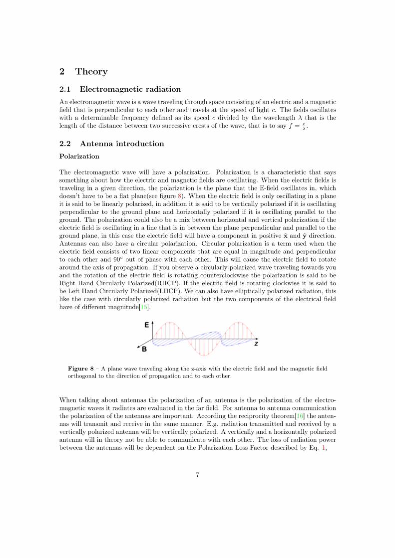
The electromagnetic wave will have a polarization. Polarization is a characteristic that sayssomething about how the electric and magnetic fields are oscillating. When the electric fields istraveling in a given direction, the polarization is the plane that the E-field oscillates in, whichdoesn’t have to be a flat plane(see figure 8). When the electric field is only oscillating in a planeit is said to be linearly polarized, in addition it is said to be vertically polarized if it is oscillatingperpendicular to the ground plane and horizontally polarized if it is oscillating parallel to theground. The polarization could also be a mix between horizontal and vertical polarization if theelectric field is oscillating in a line that is in between the plane perpendicular and parallel to theground plane, in this case the electric field will have a component in positive x and y direction.Antennas can also have a circular polarization. Circular polarization is a term used when theelectric field consists of two linear components that are equal in magnitude and perpendicularto each other and 90 out of phase with each other. This will cause the electric field to rotatearound the axis of propagation. If you observe a circularly polarized wave traveling towards youand the rotation of the electric field is rotating counterclockwise the polarization is said to beRight Hand Circularly Polarized(RHCP). If the electric field is rotating clockwise it is said tobe Left Hand Circularly Polarized(LHCP). We can also have elliptically polarized radiation, thislike the case with circularly polarized radiation but the two components of the electrical fieldhave of different magnitude[15].

Figure 8 – A plane wave traveling along the z-axis with the electric field and the magnetic fieldorthogonal to the direction of propagation and to each other.

When talking about antennas the polarization of an antenna is the polarization of the electro-magnetic waves it radiates are evaluated in the far field. For antenna to antenna communicationthe polarization of the antennas are important. According the reciprocity theorem[16] the anten-nas will transmit and receive in the same manner. E.g. radiation transmitted and received by avertically polarized antenna will be vertically polarized. A vertically and a horizontally polarizedantenna will in theory not be able to communicate with each other. The loss of radiation powerbetween the antennas will be dependent on the Polarization Loss Factor described by Eq. 1,

7

PLF = cos2(φ). (1)

If the angle between two horizontally polarized antennas are 90 we will theoretically have zerotransmitted power and there will be no reception. In the real case there might be some trans-mittance anyway because an antenna is never strictly linearly polarized and some radiation willhave mixed polarization. There are also reflections of the transmitted wave which will change thepolarization of the emitted wave. If the angle is φ = 0 we get maximum transmittance of power.At an angle between the transmitting and receiving antennas of φ = 60 50% of the transmittedpower will be lost. For a linearly polarized antenna an incoming circularly polarized radiationthe in-phase component of the electrical field will be received while the other components willbe lost[15].

2.3 The basic principle of AoAFor angle of arrival(AoA) estimation the phase φ of the incoming electromagnetic wave signalis measured at each antenna. The phase is a term describing which state the wave has interms of its periodic oscillations of the electric and magnetic fields. If the phase of and incidentelectromagnetic wave is measured by two antennas a distance d apart, a phase shift is obtained.

The phase shift is then used to determine the angle θ of the received/transmitted signal. Theprinciple of doing the conversion of the phase difference into AoA of a wave signal is describedby Eq. 2.

θ = sin−1(λ∆φ

2πd

), (2)

where λ is the wavelength of the incoming wave signal, d is the distance between the antennas inthe array and ∆φ is the measured phase shift. Between consecutive antenna elements the phaseshifts will be expressed as φ2 − φ1, ..., φn − φn−1 for a linear antenna array of size n.

Consider a plane wave incident on two antennas with a spacing of d between them. The distancer between the two antennas if looking at the projection of them on the plane parallel to theincoming wave can be described by r = d cos(θ) where θ is the angle between the incoming waveand the array. The distance r can also be calculated with the phase shift ∆φ as r = λ∆φ

2π .

For the basic principle of angle of arrival to work correctly and with robustness a few requirementsneed to be met. We need to be able to assume that the incoming wave is planar. For this to betrue the distance DTX,RX from the source of the incoming signal to the center of the antennaarray need to be DTX,RX >> λ. In this case a distance ten times that of the wavelength can beseen as much larger than the wavelength. So with objects closer than about one meter to theantenna array we can get problems with the accuracy of the angle measurement.

Another thing that you need to take into account is the sampling theorem. The sampling theoremstates that a signal has to be sampled with twice the frequency of the original signal[18]. Forantenna arrays this means that there is a maximum distance the antenna elements can be fromeach other. To avoid aliasing problems the spacing d between the antennas in the array are notallowed to differ more then d = λ

2 [19]. Aliasing is an effect that causes the signals to become

8

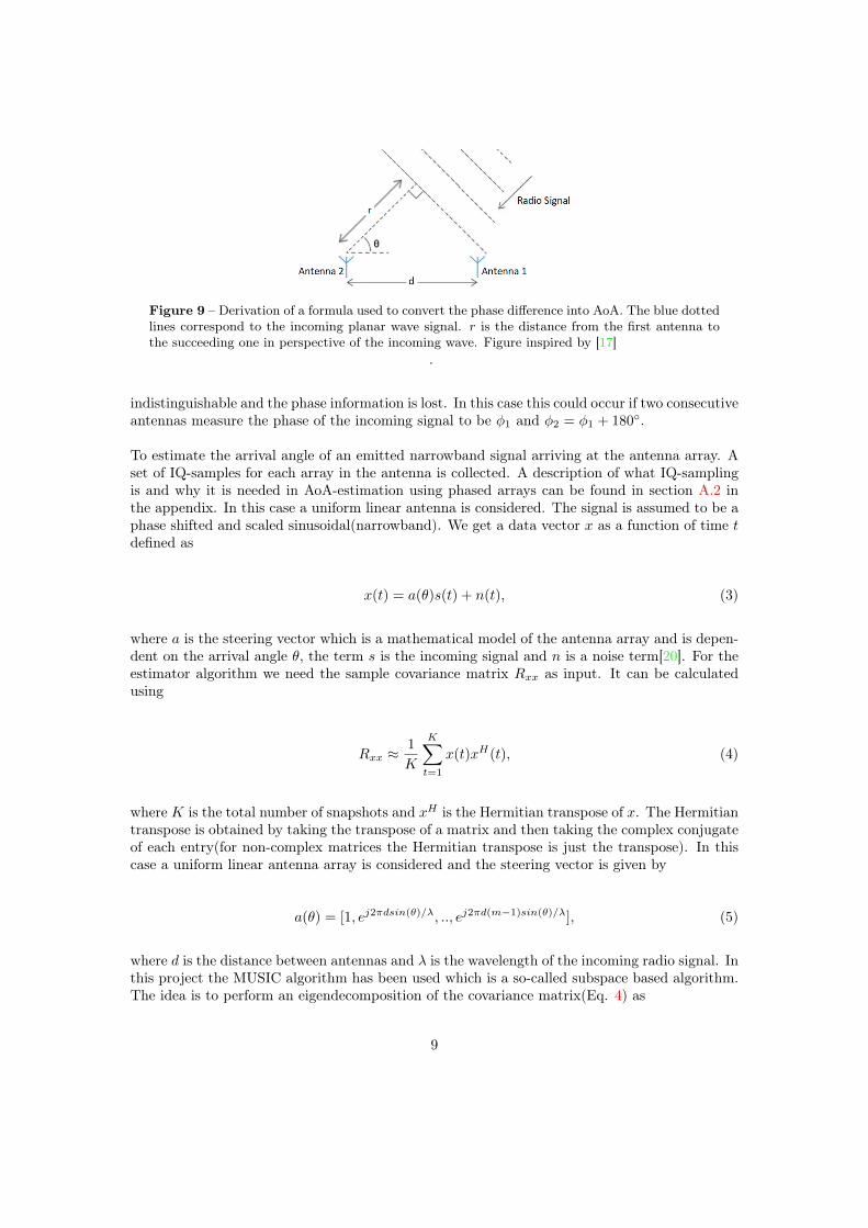
Figure 9 – Derivation of a formula used to convert the phase difference into AoA. The blue dottedlines correspond to the incoming planar wave signal. r is the distance from the first antenna tothe succeeding one in perspective of the incoming wave. Figure inspired by [17]

.

indistinguishable and the phase information is lost. In this case this could occur if two consecutiveantennas measure the phase of the incoming signal to be φ1 and φ2 = φ1 + 180.

To estimate the arrival angle of an emitted narrowband signal arriving at the antenna array. Aset of IQ-samples for each array in the antenna is collected. A description of what IQ-samplingis and why it is needed in AoA-estimation using phased arrays can be found in section A.2 inthe appendix. In this case a uniform linear antenna is considered. The signal is assumed to be aphase shifted and scaled sinusoidal(narrowband). We get a data vector x as a function of time tdefined as

x(t) = a(θ)s(t) + n(t), (3)

where a is the steering vector which is a mathematical model of the antenna array and is depen-dent on the arrival angle θ, the term s is the incoming signal and n is a noise term[20]. For theestimator algorithm we need the sample covariance matrix Rxx as input. It can be calculatedusing

Rxx ≈ 1

K

K∑t=1

x(t)xH(t), (4)

where K is the total number of snapshots and xH is the Hermitian transpose of x. The Hermitiantranspose is obtained by taking the transpose of a matrix and then taking the complex conjugateof each entry(for non-complex matrices the Hermitian transpose is just the transpose). In thiscase a uniform linear antenna array is considered and the steering vector is given by

a(θ) = [1, ej2πdsin(θ)/λ, .., ej2πd(m−1)sin(θ)/λ], (5)

where d is the distance between antennas and λ is the wavelength of the incoming radio signal. Inthis project the MUSIC algorithm has been used which is a so-called subspace based algorithm.The idea is to perform an eigendecomposition of the covariance matrix(Eq. 4) as

9

Rxx = V AV H , (6)

where A is a diagonal matrix containing the eigenvalues of Rxx(Eq. 4) and V contains thecorresponding eigenvectors. The output power of an antenna array is measured by

p(w) = wHRxxw, (7)

where w is a vector of weights[21]. These weights are different depending on the method used.The method we have used is the Capon’s Beamformer[22] and the weights are given by

w =R−1xx a(θ)

aH(θ)R−1xx a(θ)

, (8)

which will result in the following spatial power spectrum[21]

P (θ) =1

aH(θ)R−1xx a(θ)

. (9)

Under the assumption that the eigenvalues of the signal Vs is much larger than the eigenvaluesof the noise Vn the eigenvectors can be sorted and Eq. 6 can be written as

Rxx = VsAVHs + σVnV

Hn , (10)

where σ is the eigenvalue of the eigenvectors Vn. Vn is orthogonal to the angle of incidence θas V Hn a(θ) = 0. The orthogonal projector onto the noise subspace is estimated as VnV Hn . Weobtain the MUSIC “spatial spectrum” by putting VnV Hn as an estimation for Rxx in Eq. 9. TheMUSIC “spatial spectrum” is defined as [21]

P (θ) =1

aH(θ)VnV Hn a(θ). (11)

The largest peak in the spatial spectrum corresponds to the angle of arrival. The angle of arrivalis then determined by finding the largest peak of the pseudo-spectrum[13]. This is done bylooping through the desired values of θ.

10

2.4 Antenna array design considerationsMutual coupling

Mutual coupling is the electromagnetic interaction between individual antenna elements in anantenna array. The current induced in each antenna element is mainly dependent on the antennaelements own excitation but also on the contribution of adjacent antenna elements. Mutualcoupling causes changes in the radiation pattern of the array as well as the input impedance ofeach antenna element in the array. The changes in the radiation pattern can be used for beamforming but could also cause problems such as spots with low reception. The mutual couplingis inversely proportional to the distance between each antenna element. To characterize mutualcoupling it is possible to utilize mutual impedance or S-parameters to form a coupling matrixused for compensation in the data processing. Mutual coupling between antenna elements is oneof the most important parameters to take into consideration when designing an antenna array.So we want to minimize the power transmitted between antenna elements in the array. We cando this by increasing the distance d between the antenna elements, thus making the whole arraylarger by a factor of d×N−1 where N is the number of antenna elements in the array. We couldalso in general increase the frequency. This project is however bound to the Bluetooth regime inthe electromagnetic frequency spectrum. What we have left is to decrease the reception betweenthe antenna elements by focusing on the gain. The gain of an antenna will not be the same inevery direction, by rotating the antenna elements in relation to each other so that the part of theradiation patterns with the minimum gain is pointed towards each other. This could potentiallydecrease the mutual coupling between antenna elements by a substantial amount.

Another important problem is that we can have a phase center of the antenna that is notconstant. The phase center of an antenna is defined as the center of where radiation is comingfrom and where measurements are done. In this report when we are talking about the distance dbetween antennas what we are actually meaning is the distance between the phase centers of eachantenna. The phase center can change depending on angle of incidence or signal strength butalso on frequency. To get a measured phase with a low error the antenna used in antenna arraysshould have a fixed phase center. If the phase center is moving depending on characteristics ofthe incoming wave this need to be compensated for in the post processing of the measured data.Running direction finding algorithm is however computationally intensive and demand plenty ofRAM and Flash memory. The development of better and cheaper RAM and Flash memorieshave opened up a larger customer group for AoA applications. Frequency is not important forus, because we will always look at the same frequency as AoA is based on a single wavelength.It is important to keep down manufacturing costs of the array to be able to compete on themarket. Bluetooth devices are known to be of small size and with a compact design. Thus, forthe antenna array to be appealing for the customer as a Bluetooth device the array should also besmall. A small size will increase the challenges for the design of the antenna array because of theincreased mutual coupling that comes with small distances between the antenna elements[23].

11

Phase center

The phase center is defined as the apparent source of radiation. If the source were ideal it wouldhave a spherical equiphase contour, but the real case is slightly different, because the equiphasecontour is irregular and each segment has its own apparent radiation origin. Thus the phasecenter of an antenna is not only angle dependent (elevation and azimuth) but also it depends onthe signal frequency[24]. To get a good phase all intentional phase shifts of the signal should beremoved. The radio wave packet must contain a section of constant tone with whitening disabledwhere there are no phase-shifts caused by modulation. The phase center of the antenna must beconstant to get a good estimation of the AoA. If the phase center change due to the directionof the incoming wave signal this has to be accounted for in the post processing algorithm. Theposition of the antenna phase center is not necessarily the geometric center of the antenna. Thephase center is not constant but depends on the direction the radio signal is coming in.

3 Method

3.1 Simulation procedureThe commercial electromagnetics simulator program CST studio suite have been used to in-vestigate the different characteristics of the Niche antenna. It has also been used to simulatehow different configurations of an antenna array are affecting the individual antenna elements interms of mutual coupling and isolation. We have also done direct phase measurements with asingle Niche antenna as well as with an antenna array prototype utilizing plane wave excitationin CST.

3.1.1 Niche antenna characteristics

Extensive simulations on the Niche antenna have been accomplished in order to learn about itscharacteristics. Characteristics such as radiation pattern, mutual coupling and different geome-tries of the PCB and the antenna cutout. In these simulations we have had two capacitors onthe Niche antenna with the feed configured to be over the lower capacitance.

To get a measure of the isolation between two or more antenna elements we look at how muchof the radiation, that one or more antennas is sending out, is received under testing. With otherwords a lower value in dB is better. Initially we were aiming at a mutual coupling of maximum-10 dB. This corresponds to a radio transmittance of only 10% and can be considered to be agood benchmark value for a low mutual coupling. When simulating different configurations ofan antenna array consisting of Niche antenna elements we started by adding an inactive Nicheantenna next to the active one, before making both active. We proceeded to experiment withthe spacing between the antennas and orientation of them in relation to each other while lookingat the mutual coupling in terms of the S-parameter. This test was done with the two antennaspositioned on a PCB edge on two different PCBs. The same test was also done with two ormore antennas positioned on the same PCB. The mutual coupling in terms of the S-parameterwas analyzed with different modifications to the PCB ground plane such as slits and differentshapes of the PCB such as rectangular, dodecagonal or circular PCBs. We also tried stackingthe antenna utilizing multiple PCBs. Figures describing examples of the model when simulatingantenna stacking can be seen in figure A.9 in appendix. Investigation of stacking multiple antennaarrays showed to be viable with mutual coupling in mind. The results are not used in this projectbut could be used for future development, see figure A.11 in the appendix.

12

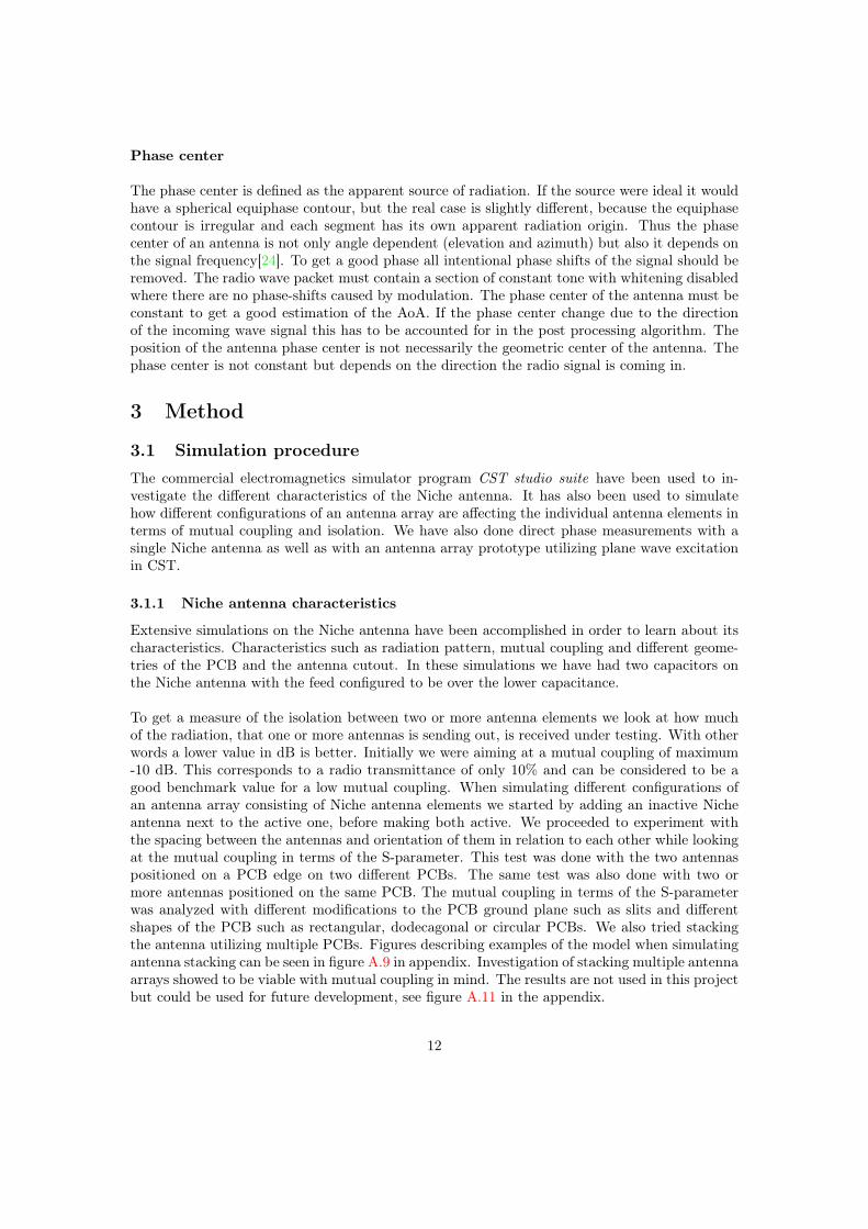
After a lot of testing we found an antenna array design that seemed to work well both in termsof isolation between the antenna elements i.e. mutual coupling between them and the size ofthe array. The antenna array that has been developed is 60×60 mm and consists of four Nicheantennas positioned on each side of a quadratic PCB. To be able to simulate the antenna arrayin action doing phase measurements the plane wave excitation functionality in CST has beenused. We have been working in the frequency domain because this is what was available atthe moment. The frequency domain solver in CST uses the finite element method to solve theMaxwell’s equations. The simulation is done by sending a plane wave from a fixed direction whilemeasuring the phase at each antenna element. If another angle of incidence of the plane wave isdesired the antenna array can be rotated around its center. The plane wave will induce currentsin the antenna ground plane. The induced currents will be measured at the feeding point of eachantenna element. For the simulation it does not matter which angle you chose to send the planewave from. To get consistent results the original angle should however not be changed if youwant to move the AUT between measurements. It was noted that when moving or changing theantenna under test(and thus changing the boundary conditions in CST) between simulations theresults of the measured phase might be inconsistent. That is because the plane wave in CST isexcited at the boundary. To get consistent results this was solved by adding a "border structure"around the model in CST and the boundary condition has to be set to Open. An open boundarycondition means that waves can pass this boundary freely with minimal reflections. In our casethe border structure consist of two large walls, one at each side of the model(See figure 10). Theborder structure is exempt from the meshing which makes it invisible to the incident plane wave.With this method it is possible to change, move and rotate the AUT(antenna under testing)freely within the border structure without affecting the phase measurements on the plane wave.Using this setup in CST we have done phase measurements with angle of incidence ranging from−90 to 90 for both azimuth and elevation angles. The border structures are only added inorder to keep the boundary box constant.

Figure 10 – Model in CST with border structures. A necessary part in order to do accuratephase measurements in the frequency domain in CST.

13

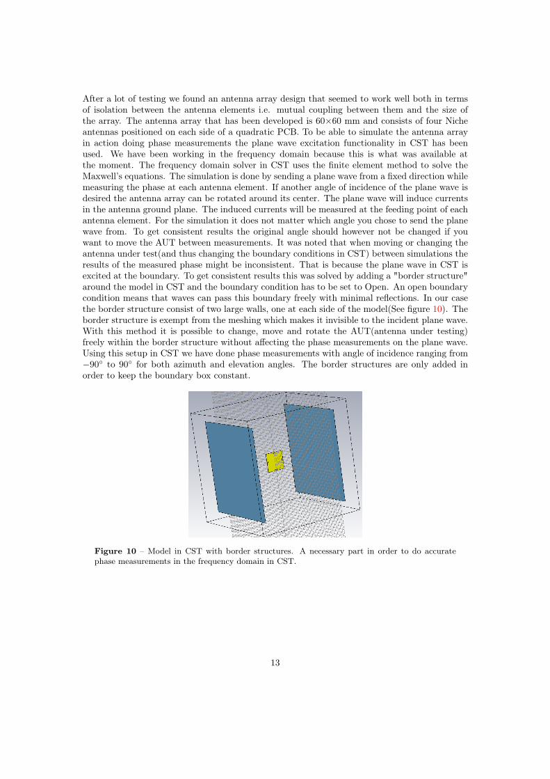
3.2 Calculation of the expected phase valueComparing simulated results or live measurements to a numerically calculated value is a goodway to confirm its validity. To calculate the expected phase value we have been looking at thegeometrical path an antenna element is experiencing between measurements and then calculatedthe expected phase shift this corresponds to. When rotating the antenna azimuthally around itscenter point, from a state 1 to a state 2 as seen in figure 11, the distance r an antenna element inthe array will experience is given by r = d

2 sin(θAzimuth) where d is the distance between oppositeantenna elements. This length is then divided by the wavelength corresponding to the frequencywe are looking at and multiplied with 360 degrees and we will get the expected relative phase.

Figure 11 – A graphical description of how an antenna element is moved when rotating theantenna array azimuthally around its center point, from a state 1 to a state 2. The distance r canbe used to calculate the expected phase shift between state 1 and 2.

3.3 Measurement procedure

3.3.1 Anechoic chamber

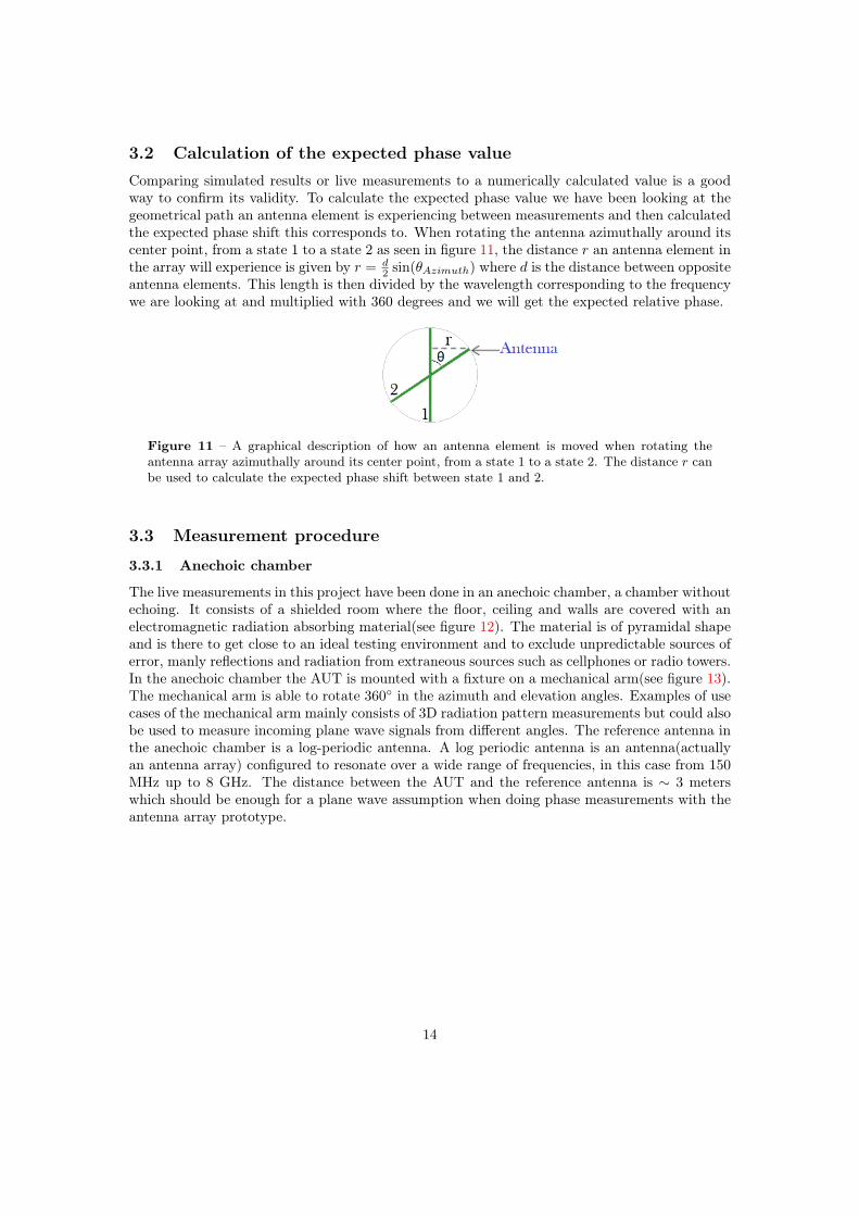
The live measurements in this project have been done in an anechoic chamber, a chamber withoutechoing. It consists of a shielded room where the floor, ceiling and walls are covered with anelectromagnetic radiation absorbing material(see figure 12). The material is of pyramidal shapeand is there to get close to an ideal testing environment and to exclude unpredictable sources oferror, manly reflections and radiation from extraneous sources such as cellphones or radio towers.In the anechoic chamber the AUT is mounted with a fixture on a mechanical arm(see figure 13).The mechanical arm is able to rotate 360 in the azimuth and elevation angles. Examples of usecases of the mechanical arm mainly consists of 3D radiation pattern measurements but could alsobe used to measure incoming plane wave signals from different angles. The reference antenna inthe anechoic chamber is a log-periodic antenna. A log periodic antenna is an antenna(actuallyan antenna array) configured to resonate over a wide range of frequencies, in this case from 150MHz up to 8 GHz. The distance between the AUT and the reference antenna is ∼ 3 meterswhich should be enough for a plane wave assumption when doing phase measurements with theantenna array prototype.

14

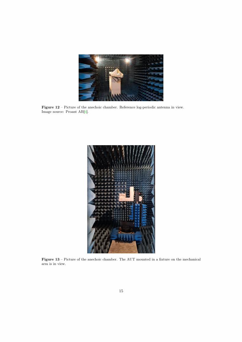
Figure 12 – Picture of the anechoic chamber. Reference log-periodic antenna in view.Image source: Proant AB[6].

Figure 13 – Picture of the anechoic chamber. The AUT mounted in a fixture on the mechanicalarm is in view.

15

3.3.2 Realization of the antenna array prototype

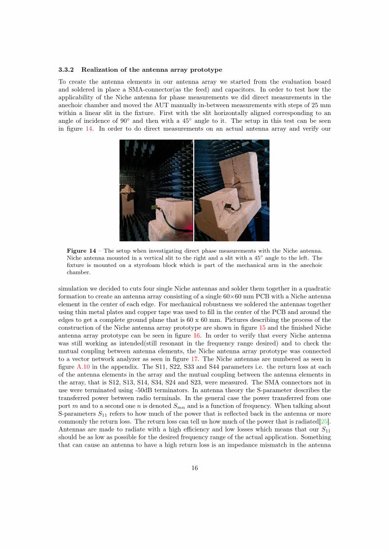
To create the antenna elements in our antenna array we started from the evaluation boardand soldered in place a SMA-connector(as the feed) and capacitors. In order to test how theapplicability of the Niche antenna for phase measurements we did direct measurements in theanechoic chamber and moved the AUT manually in-between measurements with steps of 25 mmwithin a linear slit in the fixture. First with the slit horizontally aligned corresponding to anangle of incidence of 90 and then with a 45 angle to it. The setup in this test can be seenin figure 14. In order to do direct measurements on an actual antenna array and verify our

Figure 14 – The setup when investigating direct phase measurements with the Niche antenna.Niche antenna mounted in a vertical slit to the right and a slit with a 45 angle to the left. Thefixture is mounted on a styrofoam block which is part of the mechanical arm in the anechoicchamber.

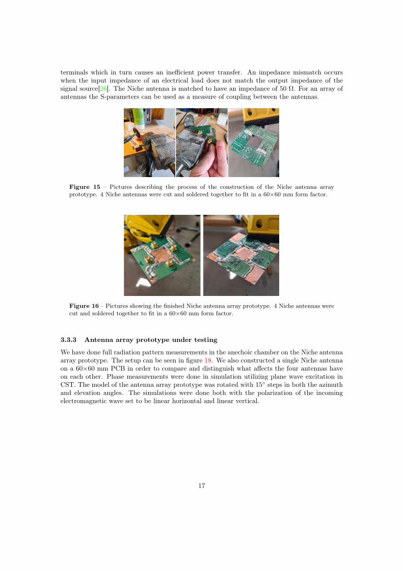
simulation we decided to cuts four single Niche antennas and solder them together in a quadraticformation to create an antenna array consisting of a single 60×60 mm PCB with a Niche antennaelement in the center of each edge. For mechanical robustness we soldered the antennas togetherusing thin metal plates and copper tape was used to fill in the center of the PCB and around theedges to get a complete ground plane that is 60 x 60 mm. Pictures describing the process of theconstruction of the Niche antenna array prototype are shown in figure 15 and the finished Nicheantenna array prototype can be seen in figure 16. In order to verify that every Niche antennawas still working as intended(still resonant in the frequency range desired) and to check themutual coupling between antenna elements, the Niche antenna array prototype was connectedto a vector network analyzer as seen in figure 17. The Niche antennas are numbered as seen infigure A.10 in the appendix. The S11, S22, S33 and S44 parameters i.e. the return loss at eachof the antenna elements in the array and the mutual coupling between the antenna elements inthe array, that is S12, S13, S14, S34, S24 and S23, were measured. The SMA connectors not inuse were terminated using -50dB terminators. In antenna theory the S-parameter describes thetransferred power between radio terminals. In the general case the power transferred from oneport m and to a second one n is denoted Smn and is a function of frequency. When talking aboutS-parameters S11 refers to how much of the power that is reflected back in the antenna or morecommonly the return loss. The return loss can tell us how much of the power that is radiated[25].Antennas are made to radiate with a high efficiency and low losses which means that our S11

should be as low as possible for the desired frequency range of the actual application. Somethingthat can cause an antenna to have a high return loss is an impedance mismatch in the antenna

16

terminals which in turn causes an inefficient power transfer. An impedance mismatch occurswhen the input impedance of an electrical load does not match the output impedance of thesignal source[26]. The Niche antenna is matched to have an impedance of 50 Ω. For an array ofantennas the S-parameters can be used as a measure of coupling between the antennas.

Figure 15 – Pictures describing the process of the construction of the Niche antenna arrayprototype. 4 Niche antennas were cut and soldered together to fit in a 60×60 mm form factor.

Figure 16 – Pictures showing the finished Niche antenna array prototype. 4 Niche antennas werecut and soldered together to fit in a 60×60 mm form factor.

3.3.3 Antenna array prototype under testing

We have done full radiation pattern measurements in the anechoic chamber on the Niche antennaarray prototype. The setup can be seen in figure 18. We also constructed a single Niche antennaon a 60×60 mm PCB in order to compare and distinguish what affects the four antennas haveon each other. Phase measurements were done in simulation utilizing plane wave excitation inCST. The model of the antenna array prototype was rotated with 15 steps in both the azimuthand elevation angles. The simulations were done both with the polarization of the incomingelectromagnetic wave set to be linear horizontal and linear vertical.

17

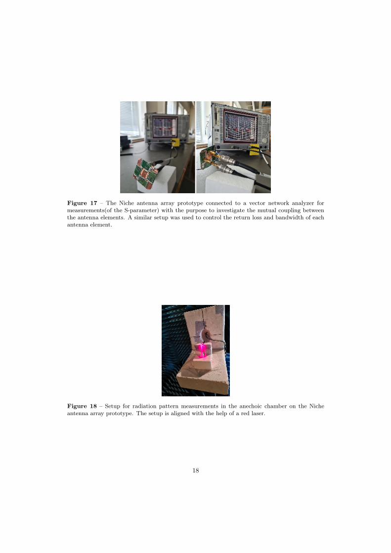
Figure 17 – The Niche antenna array prototype connected to a vector network analyzer formeasurements(of the S-parameter) with the purpose to investigate the mutual coupling betweenthe antenna elements. A similar setup was used to control the return loss and bandwidth of eachantenna element.

Figure 18 – Setup for radiation pattern measurements in the anechoic chamber on the Nicheantenna array prototype. The setup is aligned with the help of a red laser.

18

3.3.4 Cable switch

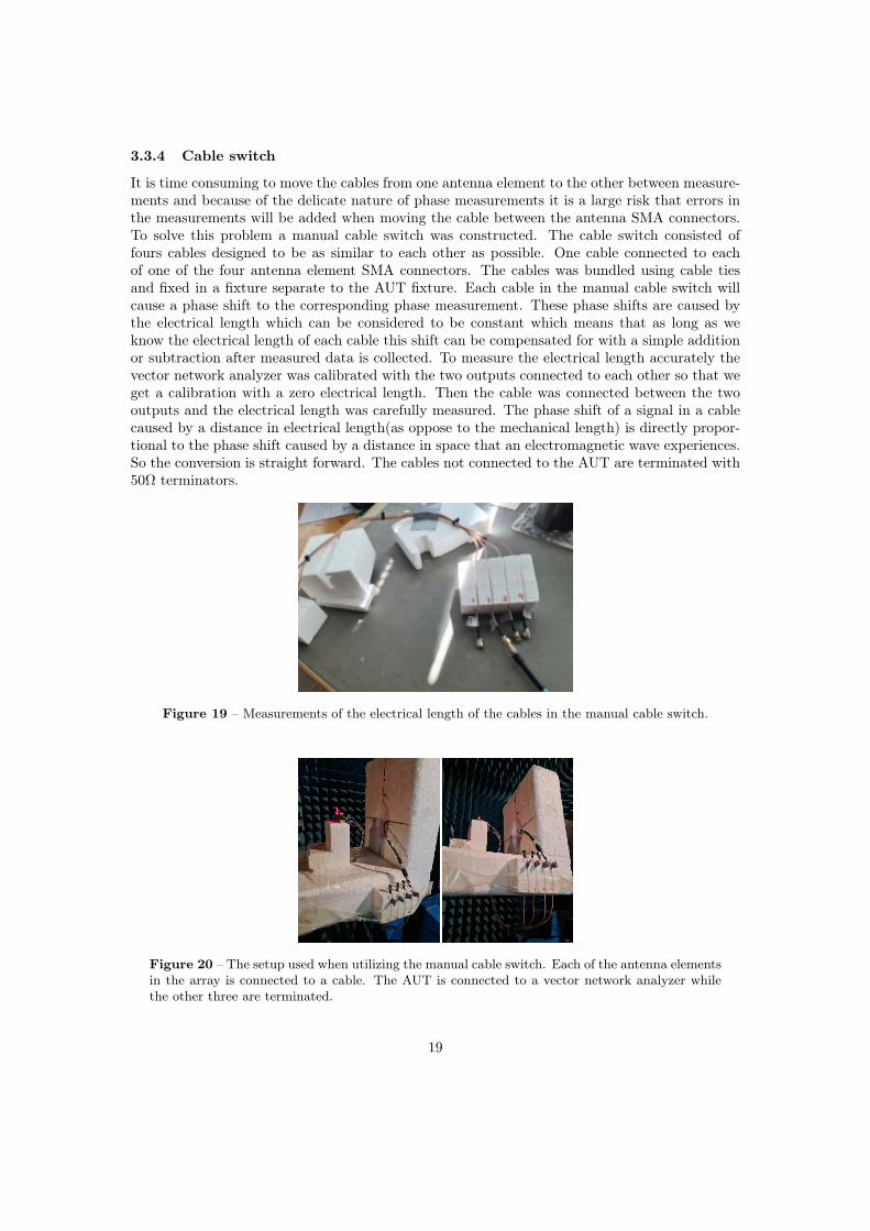
It is time consuming to move the cables from one antenna element to the other between measure-ments and because of the delicate nature of phase measurements it is a large risk that errors inthe measurements will be added when moving the cable between the antenna SMA connectors.To solve this problem a manual cable switch was constructed. The cable switch consisted offours cables designed to be as similar to each other as possible. One cable connected to eachof one of the four antenna element SMA connectors. The cables was bundled using cable tiesand fixed in a fixture separate to the AUT fixture. Each cable in the manual cable switch willcause a phase shift to the corresponding phase measurement. These phase shifts are caused bythe electrical length which can be considered to be constant which means that as long as weknow the electrical length of each cable this shift can be compensated for with a simple additionor subtraction after measured data is collected. To measure the electrical length accurately thevector network analyzer was calibrated with the two outputs connected to each other so that weget a calibration with a zero electrical length. Then the cable was connected between the twooutputs and the electrical length was carefully measured. The phase shift of a signal in a cablecaused by a distance in electrical length(as oppose to the mechanical length) is directly propor-tional to the phase shift caused by a distance in space that an electromagnetic wave experiences.So the conversion is straight forward. The cables not connected to the AUT are terminated with50Ω terminators.

Figure 19 – Measurements of the electrical length of the cables in the manual cable switch.

Figure 20 – The setup used when utilizing the manual cable switch. Each of the antenna elementsin the array is connected to a cable. The AUT is connected to a vector network analyzer whilethe other three are terminated.

19

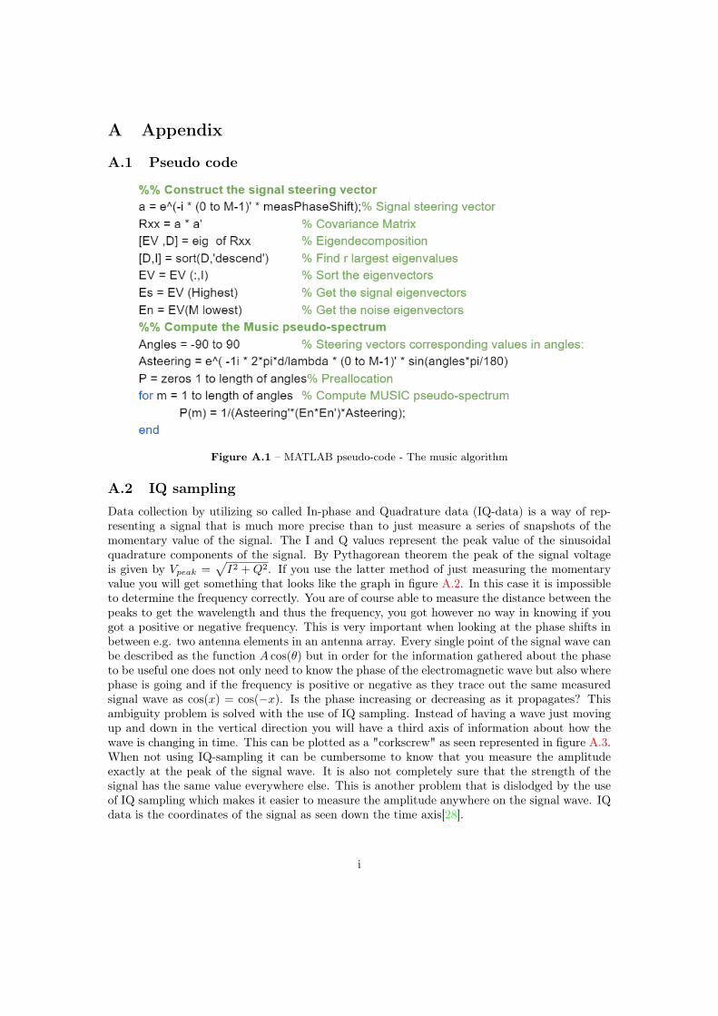
3.4 Post processing and the AoA AlgorithmIn this project we have developed a code in MATLAB utilizing the MUSIC algorithm. Thetheory behind the algorithm is described in the previous chapter. The algorithm is described indetail through a pseudo-code in figure A.1 in the appendix. In the beginning of the algorithma steering vector is stated. The steering vector contains all necessary information about howthe antenna array is configured, how the geometry of the antenna array is designed and howthe individual antenna elements are oriented. In the steering vector compensation for knownconstant phase shifts in e.g antenna elements or in circuitry and cables can be compensated forwith a simple addition or subtraction of the known error. In order to do this a subspace basedalgorithm called the MUSIC (MUltiple SIgnal Classification) algorithm is used. The algorithmtakes the measured signal at each antenna element in the array and creates a steering vector thatcontains information about the geometrical formation of the antenna array and the orientationof the antenna elements. It also deals with the decomposition of correlation matrix into twoorthogonal matrices, signal-subspace and noise-subspace[27].

The MATLAB code we have made was originally created in order to validate the phase mea-surements done with the Niche antenna array prototype. It was however more clear to directlycalculate the expected phase shifts and make comparison to what we measure or simulate. Thecreation of the code has been helpful in order to understand how a finished AoA application willoperate and how the algorithm works. The angle of arrival algorithm has been tested with madeup phase values corresponding to a certain angle. The algorithm works as intended. In order toutilize all antennas when calculating both incident azimuth and elevation angles a principle ofdivision was used. The principle of division utilizes the symmetry of our Niche antenna array andis built on the fact that the value of the actual phase in the center between two measurementswill be equal to the addition of the two phase measurements divided by 2. This was done inorder to get 3 phase measure points in a row in each direction in our algorithm. If we look atantenna 1 and 4 we will have two measure points for the phase. We want at least 3 measurepoints for the phase in order to get good accuracy so we take the values of antenna 2 and 3 andadd them together and divide by 2 to get the value of the phase at the center between antenna2 and 3 which is also the center between antenna 1 and 4 due to symmetry.

20

4 Results

In this section the results of this thesis about the applicability of the Niche antenna in an antennaarray for the purpose of direction finding are presented in text and graphics. Simulation results ofthe antenna array and direct phase measurements with the antenna array prototype in simulationare shown. The results of the measurements in the anechoic chamber and with the vector networkanalyzer of the Niche antenna and the realized antenna array prototype are presented.

4.1 Antenna array configurationAfter careful considerations acknowledged by looking at the radiation pattern and the orientationof the of the Niche antenna elements with the mutual coupling in mind, as well as after simulationsof different shapes of the antenna array we decided for a formation that works well. It consists offour Niche antennas(linearly polarized) with a 90 rotation between each consecutive antennas.This means that we will have two antenna elements with vertical polarization and two antennaelements with horizontal polarization.

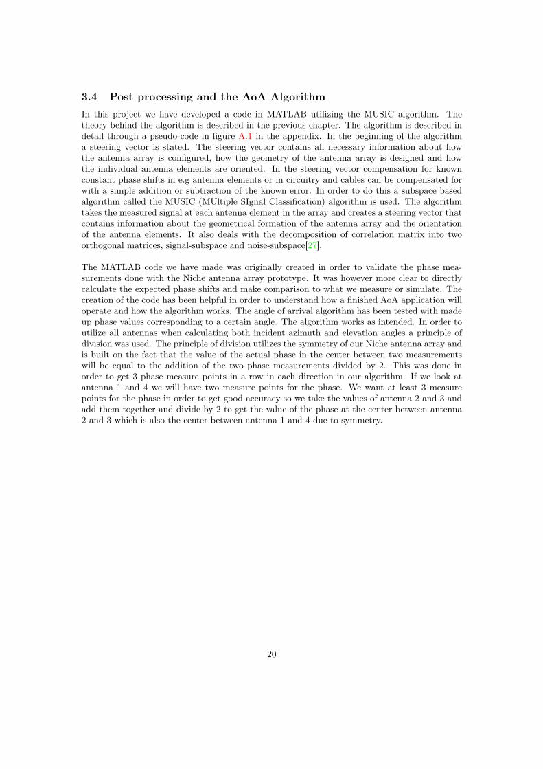
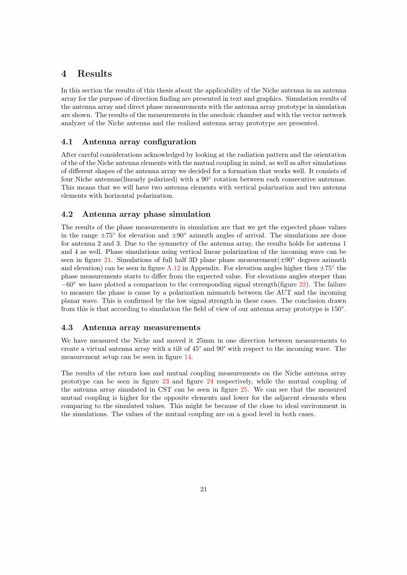
4.2 Antenna array phase simulationThe results of the phase measurements in simulation are that we get the expected phase valuesin the range ±75 for elevation and ±90 azimuth angles of arrival. The simulations are donefor antenna 2 and 3. Due to the symmetry of the antenna array, the results holds for antenna 1and 4 as well. Phase simulations using vertical linear polarization of the incoming wave can beseen in figure 21. Simulations of full half 3D plane phase measurement(±90 degrees azimuthand elevation) can be seen in figure A.12 in Appendix. For elevation angles higher then ±75 thephase measurements starts to differ from the expected value. For elevations angles steeper than−60 we have plotted a comparison to the corresponding signal strength(figure 22). The failureto measure the phase is cause by a polarization mismatch between the AUT and the incomingplanar wave. This is confirmed by the low signal strength in these cases. The conclusion drawnfrom this is that according to simulation the field of view of our antenna array prototype is 150.

4.3 Antenna array measurementsWe have measured the Niche and moved it 25mm in one direction between measurements tocreate a virtual antenna array with a tilt of 45° and 90° with respect to the incoming wave. Themeasurement setup can be seen in figure 14.

The results of the return loss and mutual coupling measurements on the Niche antenna arrayprototype can be seen in figure 23 and figure 24 respectively, while the mutual coupling ofthe antenna array simulated in CST can be seen in figure 25. We can see that the measuredmutual coupling is higher for the opposite elements and lower for the adjacent elements whencomparing to the simulated values. This might be because of the close to ideal environment inthe simulations. The values of the mutual coupling are on a good level in both cases.

21

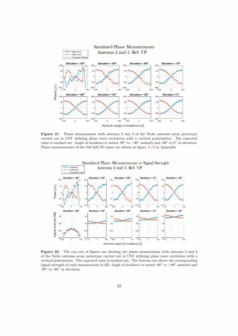
Figure 21 – Phase measurement with antenna 2 and 3 of the Niche antenna array prototypecarried out in CST utilizing plane wave excitation with a vertical polarization. The expectedvalue is marked out. Angle of incidence is varied -90 to +90 azimuth and -90 to 0 in elevation.Phase measurements of the full half 3D plane are shown in figure A.12 in Appendix

Figure 22 – The top row of figures are showing the phase measurement with antenna 2 and 3of the Niche antenna array prototype carried out in CST utilizing plane wave excitation with avertical polarization. The expected value is marked out. The bottom row shows the correspondingsignal strength of each measurement in dB. Angle of incidence is varied -90 to +90 azimuth and-90 to -60 in elevation.

22

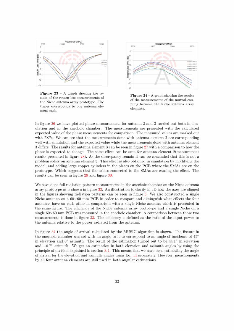
Figure 23 – A graph showing the re-sults of the return loss measurements ofthe Niche antenna array prototype. Thetraces corresponds to one antenna ele-ment each.

Figure 24 – A graph showing the resultsof the measurements of the mutual cou-pling between the Niche antenna arrayelements.

In figure 26 we have plotted phase measurements for antenna 2 and 3 carried out both in sim-ulation and in the anechoic chamber. The measurements are presented with the calculatedexpected value of the phase measurements for comparison. The measured values are marked outwith "X"s. We can see that the measurements done with antenna element 2 are correspondingwell with simulation and the expected value while the measurements done with antenna element3 differs. The results for antenna element 3 can be seen in figure 27 with a comparison to how thephase is expected to change. The same effect can be seen for antenna element 2(measurementresults presented in figure 28). As the discrepancy remain it can be concluded that this is not aproblem solely on antenna element 3. This effect is also obtained in simulation by modifying themodel, and adding large copper cylinders in the places on the PCB where the SMAs are on theprototype. Which suggests that the cables connected to the SMAs are causing the effect. Theresults can be seen in figure 29 and figure 30.

We have done full radiation pattern measurements in the anechoic chamber on the Niche antennaarray prototype as is shown in figure 32. An illustration to clarify in 3D how the axes are alignedin the figures showing radiation patterns can be seen in figure 5. We also constructed a singleNiche antenna on a 60×60 mm PCB in order to compare and distinguish what effects the fourantennas have on each other in comparison with a single Niche antenna which is presented inthe same figure. The efficiency of the Niche antenna array prototype and a single Niche on asingle 60×60 mm PCB was measured in the anechoic chamber. A comparison between those twomeasurements is done in figure 33. The efficiency is defined as the ratio of the input power tothe antenna relative to the power radiated from the antenna.

In figure 34 the angle of arrival calculated by the MUSIC algorithm is shown. The fixture inthe anechoic chamber was set with an angle to it to correspond to an angle of incidence of 45in elevation and 0 azimuth. The result of the estimation turned out to be 44.1 in elevationand −0.7 azimuth. We get an estimation in both elevation and azimuth angles by using theprinciple of division explained in section 3.4. This means that we have been estimating the angleof arrival for the elevation and azimuth angles using Eq. 11 separately. However, measurementsby all four antenna elements are still used in both angular estimations.

23

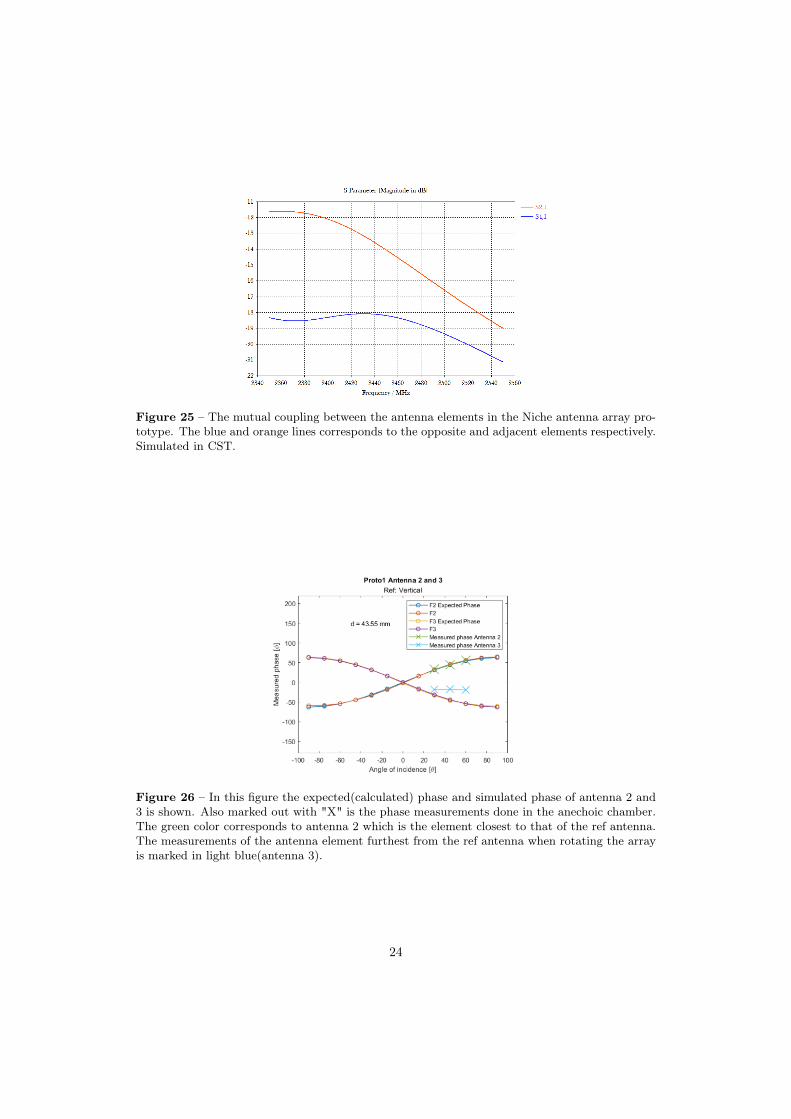
Figure 25 – The mutual coupling between the antenna elements in the Niche antenna array pro-totype. The blue and orange lines corresponds to the opposite and adjacent elements respectively.Simulated in CST.

Figure 26 – In this figure the expected(calculated) phase and simulated phase of antenna 2 and3 is shown. Also marked out with "X" is the phase measurements done in the anechoic chamber.The green color corresponds to antenna 2 which is the element closest to that of the ref antenna.The measurements of the antenna element furthest from the ref antenna when rotating the arrayis marked in light blue(antenna 3).

24

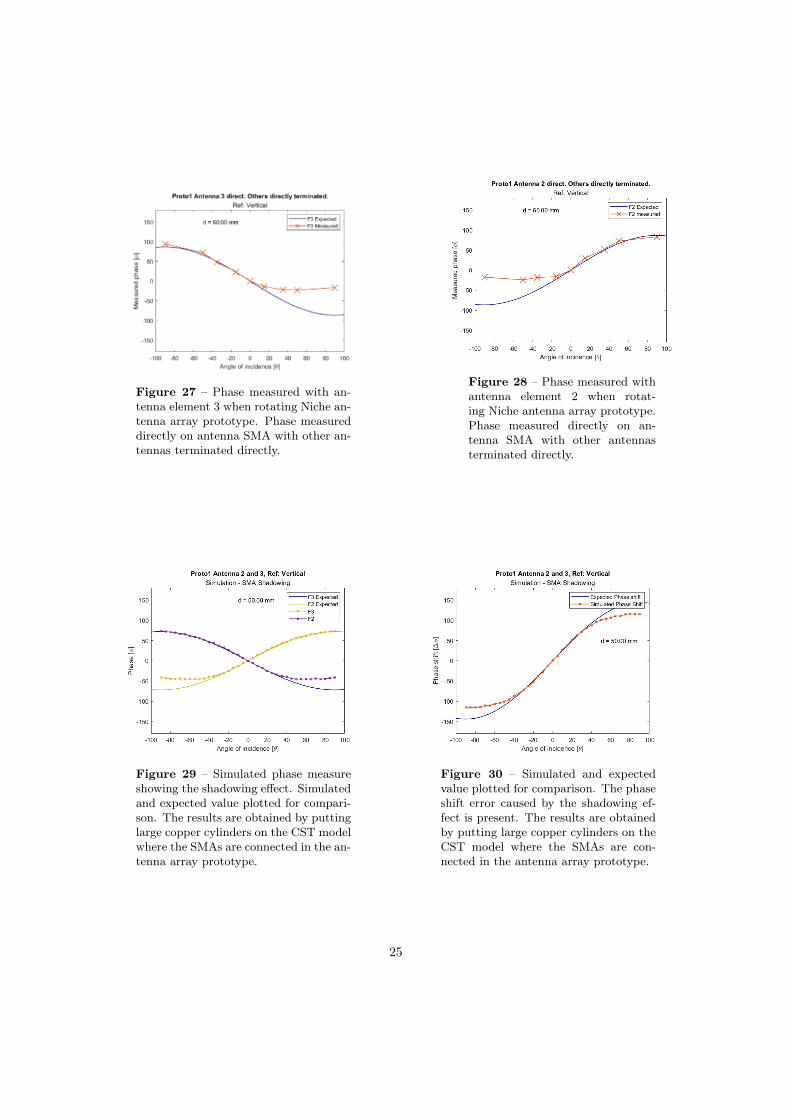
Figure 27 – Phase measured with an-tenna element 3 when rotating Niche an-tenna array prototype. Phase measureddirectly on antenna SMA with other an-tennas terminated directly.

Figure 28 – Phase measured withantenna element 2 when rotat-ing Niche antenna array prototype.Phase measured directly on an-tenna SMA with other antennasterminated directly.

Figure 29 – Simulated phase measureshowing the shadowing effect. Simulatedand expected value plotted for compari-son. The results are obtained by puttinglarge copper cylinders on the CST modelwhere the SMAs are connected in the an-tenna array prototype.

Figure 30 – Simulated and expectedvalue plotted for comparison. The phaseshift error caused by the shadowing ef-fect is present. The results are obtainedby putting large copper cylinders on theCST model where the SMAs are con-nected in the antenna array prototype.

25

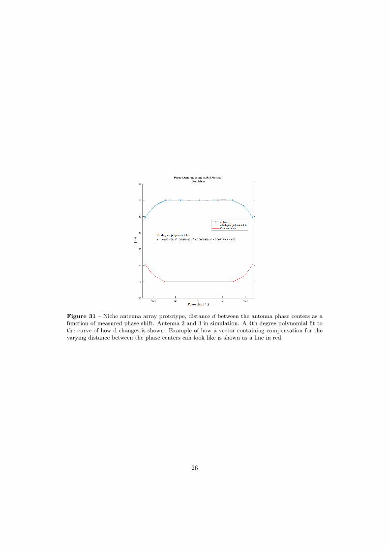
Figure 31 – Niche antenna array prototype, distance d between the antenna phase centers as afunction of measured phase shift. Antenna 2 and 3 in simulation. A 4th degree polynomial fit tothe curve of how d changes is shown. Example of how a vector containing compensation for thevarying distance between the phase centers can look like is shown as a line in red.

26

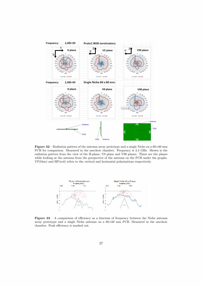
Figure 32 – Radiation pattern of the antenna array prototype and a single Niche on a 60×60 mmPCB for comparison. Measured in the anechoic chamber. Frequency is 2.4 GHz. Shown is theradiation pattern from the view of the H-plane, V0 plane and V90 planes. These are the planeswhile looking at the antenna from the perspective of the antenna on the PCB under the graphs.VP(blue) and HP(red) refers to the vertical and horizontal polarizations respectively.

Figure 33 – A comparison of efficiency as a function of frequency between the Niche antennaarray prototype and a single Niche antenna on a 60×60 mm PCB. Measured in the anechoicchamber. Peak efficiency is marked out.

27

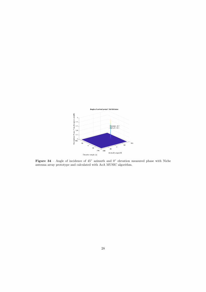
Figure 34 – Angle of incidence of 45 azimuth and 0 elevation measured phase with Nicheantenna array prototype and calculated with AoA MUSIC algorithm.

28

5 Discussion

The analysis on of the Niche antenna gave a lot of new knowledge and understanding of howthe antenna behaves and how different PCB formations might influence the overall antennacharacterizations. When looking at the return loss measurements of the Niche antenna arrayprototype in figure 23 we can see that all elements are of similar performance and on a goodlevel. The results of the measurements of the mutual coupling seen figure 24 is also on a promisinglevel. We are aiming at a benchmark for the mutual coupling to not go above -10dB. The mutualcoupling in the array is generally around -14dB with the highest coupling being between adjacentantenna elements. This also correspond well with simulation(figure 25).

In figure 34 the angle of arrival calculated by the MUSIC algorithm is shown. The fixture inthe anechoic chamber was set with an angle to it to correspond to an angle of incidence of 45in elevation and 0 azimuth. The result of the estimation turned out to be 44.1 in elevationand −0.7 azimuth. From these results we can say that the MUSIC algorithm written is ableto estimate the angle of arrival of an incoming wave using the antenna array prototype. Tosay anything about how well the antenna array works for other angles and how robust themeasurements are, more testing is needed.

Phase measurement tests in the anechoic chamber have shown to give results that suggest thatthe antenna array is suitable for angle of arrival calculations. The accuracy of the antenna arrayphase measurements makes it possible to estimate the angle of arrival of an incoming signalwith an accuracy of ±2.7 with a certainty of one standard deviation, measured with a distanceof ∼ 3m between the AUT and the reference antenna. The accuracy was estimated by takingthe standard deviation σ2

PM of the direct phase measurements, then we calculate the standarddeviation this would correspond to in a AoA estimation by

√σ2PM + σ2

PM . The estimation wasdone like this because we did not have enough angle of arrival estimations from measured datato do an analysis of accuracy directly.

The phase simulations of the Niche antenna array show promising results. In CST we haveonly been able to do simulations with strictly linear polarization in a certain direction. Howeverin the real world use case it is almost always possible to assume mixed polarization. Whensimulating we want all antenna elements to work well for all angles of incidence for at leastsome polarization. The results of the phase simulations with vertical linear polarization of theincoming wave is shown in figure 21. It is easy to see that antenna element 2 and 3 works wellwith vertically polarized radio signals for angles of incidence between ∼-75 to ∼75 elevationand ∼90 to ∼-90 azimuth. This is expected because these elements will have a polarization thatis perpendicular to that of the incoming wave at ±90 elevation, so for angles of incidence closeto this the reception will theoretically be close to zero. They however work poorly for horizontalpolarization of the incoming wave. From these tests we can draw the conclusion the antennaarray will work well for angles of arrival in the range ±90 azimuth and ±75 in elevation. Theseresults also suggests that the field of view of our antenna array prototype is 150. The anglesoutside the range of ±75 in elevation will need further investigation. It is also possible to saythat the at least two antennas in the Niche antenna array will always have a good reception evenif the incoming signal will happen to be strictly linearly polarized.

A phenomenon we chose to call "the shadowing effect" because of the resemblance of the antennaelement furthest away from the angle of incidence to be shadowed by the other antenna elements.It causes the phase reading of said element to "flatten out" as can be seen in figure 27 and in

29

figure 28. As the phase reading only "flattens out" and nothing more dramatic happens, thephase measurements of the other antenna elements together with the shadowed element can stillbe used to estimate the angle of incidence of the incoming plane wave. It is clear that we geta shadowing effect on elements further from the reference antenna when rotating Niche antennaarray prototype. When compared to earlier measurements with the 4 cables we got the distanced between the antenna elements to be equal to 43.55 mm. Now without the cables we get a d=60mm. It seems like the cables are affecting the phase center to move it closer to the center of theantenna array. The distance d between the antenna elements will change depending directly onthe measured phase shift. So if we measure a certain phase shift we will always be able to changethe distance d in the MUSIC algorithm for the measured phase shift to give a correct result in thealgorithm. This will need to be calibrated beforehand. In figure 31 we can see that the changesin the distance d between the phase centers of the two antenna elements follows the shape of a4th degree polynomial. This polynomial can be inverted(red line in figure 31) and added to thesteering vector in the MUSIC algorithm to flatten out the changes in distance d. Two differentangles of incidence(within the half 3D-plane in front of the antenna array) will never result in anidentical phase shift, they are distinguishable and can therefor be calibrated and compensatedfor. We have been able to obtain this effect in simulation by putting large copper cylinders onthe CST model where the SMAs are connected on the antenna array prototype(see figure 29and figure 30). From this result one can draw a conclusion that the cables connected to theSMAs on the antenna array prototype are causing the shadowing affect and the problem canthen be solved by using an active RF-switch. An RF-switch may not affect the antenna array ascables connected to SMAs do. We can see that the shadowed element has a measured constantphase while angles are ranging from +20 to +90. The measured phase is changing as expectedfor angles in the range -90 to +20. This means that we will always have an element witha phase that is measured without this error. With this acknowledged it is possible to make acompensation in the phase shift in the code. We can see that the phase readings are slippingaway from the expected value for the antenna element that is furthest away the source of theincoming wave. The measured phase of the other 3 antenna elements in the same setup doesnot show this effect. This "shadowing effect" can be compensated for by adding a compensationvector for every measured phase shift. The phase shift compensation is demonstrated in figure31.

One of the most important conditions for antenna developers to take into consideration whenworking with Bluetooth devices is to keep the actual application small in size. The small size ishard to achieve when it comes to antenna arrays. If a small size of an antenna array is achievedthis will on the other hand make the device exceedingly attractive on the market. Compared toprior art in the same field antenna arrays are typically well above a size of 100×100 mm andconsists of at least 3 antennas in each direction. The concept of the antenna array that we haverealized consists of 4 antenna elements symmetrically embedded around the edges of a 60×60mm PCB and will allow for 3 measure points in each direction which is good enough in terms ofaccuracy according to known expertise.

5.1 Future DevelopmentIn this project the main goal of realizing a concept of an antenna array consisting of Niche antennaelements have been met. We have been able to prove that the Niche antenna is suitable forAoA applications in terms of mutual coupling, size and accuracy. Further development includesphase measurements and simulations which should be carried with the goal to understand howthe antenna array behaves for angles not investigated in this project. This includes testing

30

in a anechoic chamber with different polarizations and testing outside of anechoic chamber toinclude disturbance in the form of noise. Realizing the application with an actual antenna switchcould facilitate testing. Testing would then be done in knowledge that the testing equipmentand cables leading to each antenna is not disturbing the measurements. Future developmentcould also include the algorithm to be supplemented to take in measured IQ-signals, along withcompensations for undesirable phase shifts and shadowing effects in the system.

Investigation of development including adding more antennas to the array for further increasedaccuracy and range of angles possible to be estimated should also be part of future development.Because of the already small size of the array there would not be, in terms of size, a problem tostack two of them on top of each other or to add a 5th and 6th antenna element at the centerof the antenna array orthogonal to the other antenna elements. Simulation has shown very lowmutual coupling(see figure 25), which would also allow for more antenna elements to be added.In terms of mutual coupling there is a possibility of stacking as seen in figure A.11 as well.In the case of stacking transmittance through and reflections on the PCB could be a cause ofdisturbances when measuring the phase. This too is a subject of further investigation. For a flat2D-antenna array like the one made in this project it is in theory possible to estimate all anglesfrom the half-space on one side of the antenna array. We can only estimate angles from one sideof the PCB because otherwise there would be an ambiguity problem were the array would notknow if a signal is coming from e.g. 45 elevation or 225 elevation. Because the two signals willcause exactly the same phase shift. Adding one antenna element in a third direction to achievea 3D-antenna array would allow for direction finding in all angles in the 3D-plane. This additioncould increase the number of use cases of the antenna array substantially.

31

6 References

References

[1] www.ublox.com "How we built our Bluetooth direction finding demo",Available: https://www.u-blox.com/en/blogs/tech/how-we-built-our-bluetooth-direction-finding-demo, 2021-08-19.

[2] Salonen, Pekka (2001). Human Friendly Mechatronics || A Novel Antenna System for Man-Machine Interface. 37–42.

[3] Bluetooth Core Specification v5.1.Available: https://www.bluetooth.com/bluetooth-resources/bluetooth-core-specification-v5-1-feature-overview/, 2021-08-25

[4] Elhag, N. A. A., Osman, I. M., Yassin, A. A., & Ahmed, T. B. (2013). Angle of arrivalestimation in smart antenna using MUSIC method for wideband wireless communication.

[5] Rutfors, T. (2021). Patent: ANTENNA ARRANGEMENT AND A DEVICE COMPRIS-ING SUCH AN ANTENNA ARRANGEMENT. (US 10,910,715 B2).

[6] Proant AB.Available: https://proantantennas.com/niche-2400-mhz-antenna/, 2021-05-08

[7] Vallauri, Roberto; Bertin, Giorgio; Piovano, Bruno; Gianola, Paolo (2015). ElectromagneticField Zones Around an Antenna for Human Exposure Assessment: Evaluation of the humanexposure to EMFs.

[8] www.everythingrf.com "What are Near Field and Far Field Regions of an Antenna?",Available: https://www.everythingrf.com/community/what-are-near-field-and-far-field-regions-of-an-antenna, 2021-08-03.

[9] Petterson, G.; (1987) VÅGUTBREDNINGS- OCH ANTENNTEORI (EA 114)

[10] www.argenox.com "INTRODUCTION TO BLUETOOTH CLASSIC",Available: https://www.argenox.com/library/bluetooth-classic/introduction-to-bluetooth-classic/, 2021-08-19.

[11] Giovanni, P.; Fabio, A.; Yonas Engida, G.; Ilsun, Y.; (2021) Bluetooth 5.1: An Analysis ofDirection Finding Capability for High-Precision Location Services

[12] U-blox webinar "Bluetooth for High Precision Indoor Positioning",Available: https://www.u-blox.com/en/webinars-1, 2021-04-08.

[13] www.silabs.com "understanding advanced bluetooth angle estimation techniques for realtime locationing",Avalible: https://www.silabs.com/documents/public/presentations/ew-2018-understanding-advanced-bluetooth-angle-estimation-techniques-for-real-

32

time-locationing.pdf, 2021-04-08.

[14] Aghababaiyan, Keyvan; Zefreh, Reza Ghaderi; Shah-Mansouri, Vahid (2018). 3D-OMP and3D-FOMP algorithms for DOA estimation. Physical Communication, 31(), 87–95.

[15] https://www.antenna-theory.com, " Polarization of Plane Waves",Available: https://www.antenna-theory.com/basics/polarization.php, 2021-08-04.

[16] https://www.antenna-theory.com, "Reciprocity",Available: https://www.antenna-theory.com/definitions/reciprocity.php, 2021-08-19

[17] www.digikey.com "Use Bluetooth 5.1-Enabled Platforms for Precise Asset Tracking andIndoor Positioning - Part 1".Available: https://www.digikey.com/en/articles/use-bluetooth-5-1-enabled-platforms-part-1, 2021-05-28.

[18] Bernhard Preim, Charl Botha, in Visual Computing for Medicine (Second Edition), 2014

[19] Lindmark, B.; Lundgren, S.; Sanford, J.R.; Beckman, C. (1998). Dual-polarized array forsignal-processing applications in wireless communications.

[20] Eriksson, J.; Beckman, C. (1996). IEEE Antennas and Propagation Society InternationalSymposium. 1996 Digest - Plausibility of assuming ideal arrays for direction of arrival esti-mation.

[21] Krim, H.; Viberg, M. (1996). Two decades of array signal processing research: the parametricapproach. , 13(4), 67–94.

[22] Stoica, P.; Zhisong Wang, ; Jian Li, (2003). Robust Capon beamforming. IEEE SignalProcessing Letters, 10(6), 172–175.

[23] Mathworks "Mutual Coupling",Available: https://se.mathworks.com/help/antenna/ug/mutual-coupling.html, 2021-08-05

[24] www.gssc.esa.int/navipedia "Antenna Phase Centre",Available: https://gssc.esa.int/navipedia/index.php/Antenna_Phase_Centre#cite_note-1, 2021-04-07.

[25] https://www.antenna-theory.com,Available: https://www.antenna-theory.com/, 2021-05-28

[26] devsblog.microsoft.comAvailable: shorturl.at/aduGO, 2021-06-04.

[27] Optimization of MUSIC algorithm for angle of arrival estimation in wireless communicationsby M.Mohanna,Available: https://www.tandfonline.com/doi/full/10.1016/j.nrjag.2013.06.014,

33

2021-08-06

[28] www.whiteboard.ping.se "I/Q Data explained",Available: http://whiteboard.ping.se/SDR/IQ, 2021-05-28.

[29] www.hwotogeek.com "bluetooth 5.1 whats new and why it matters",Available: https://www.howtogeek.com/403606/bluetooth-5.1-whats-new-and-why-it-matters/, 2021-04-08.

[30] Singh, Hema; Sneha, H. L.; Jha, R. M. (2013). Mutual Coupling in Phased Arrays: AReview. International Journal of Antennas and Propagation, 2013(), 1–23.

34

A Appendix

A.1 Pseudo code

Figure A.1 – MATLAB pseudo-code - The music algorithm

A.2 IQ samplingData collection by utilizing so called In-phase and Quadrature data (IQ-data) is a way of rep-resenting a signal that is much more precise than to just measure a series of snapshots of themomentary value of the signal. The I and Q values represent the peak value of the sinusoidalquadrature components of the signal. By Pythagorean theorem the peak of the signal voltageis given by Vpeak =

√I2 +Q2. If you use the latter method of just measuring the momentary

value you will get something that looks like the graph in figure A.2. In this case it is impossibleto determine the frequency correctly. You are of course able to measure the distance between thepeaks to get the wavelength and thus the frequency, you got however no way in knowing if yougot a positive or negative frequency. This is very important when looking at the phase shifts inbetween e.g. two antenna elements in an antenna array. Every single point of the signal wave canbe described as the function A cos(θ) but in order for the information gathered about the phaseto be useful one does not only need to know the phase of the electromagnetic wave but also wherephase is going and if the frequency is positive or negative as they trace out the same measuredsignal wave as cos(x) = cos(−x). Is the phase increasing or decreasing as it propagates? Thisambiguity problem is solved with the use of IQ sampling. Instead of having a wave just movingup and down in the vertical direction you will have a third axis of information about how thewave is changing in time. This can be plotted as a "corkscrew" as seen represented in figure A.3.When not using IQ-sampling it can be cumbersome to know that you measure the amplitudeexactly at the peak of the signal wave. It is also not completely sure that the strength of thesignal has the same value everywhere else. This is another problem that is dislodged by the useof IQ sampling which makes it easier to measure the amplitude anywhere on the signal wave. IQdata is the coordinates of the signal as seen down the time axis[28].

i

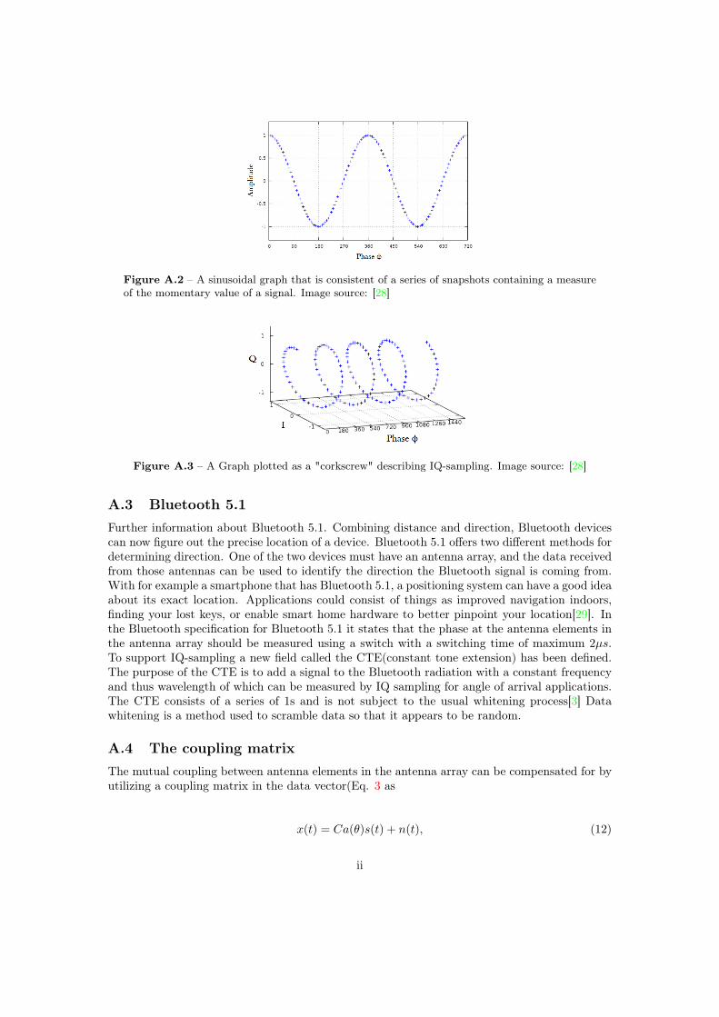
Figure A.2 – A sinusoidal graph that is consistent of a series of snapshots containing a measureof the momentary value of a signal. Image source: [28]

Figure A.3 – A Graph plotted as a "corkscrew" describing IQ-sampling. Image source: [28]

A.3 Bluetooth 5.1Further information about Bluetooth 5.1. Combining distance and direction, Bluetooth devicescan now figure out the precise location of a device. Bluetooth 5.1 offers two different methods fordetermining direction. One of the two devices must have an antenna array, and the data receivedfrom those antennas can be used to identify the direction the Bluetooth signal is coming from.With for example a smartphone that has Bluetooth 5.1, a positioning system can have a good ideaabout its exact location. Applications could consist of things as improved navigation indoors,finding your lost keys, or enable smart home hardware to better pinpoint your location[29]. Inthe Bluetooth specification for Bluetooth 5.1 it states that the phase at the antenna elements inthe antenna array should be measured using a switch with a switching time of maximum 2µs.To support IQ-sampling a new field called the CTE(constant tone extension) has been defined.The purpose of the CTE is to add a signal to the Bluetooth radiation with a constant frequencyand thus wavelength of which can be measured by IQ sampling for angle of arrival applications.The CTE consists of a series of 1s and is not subject to the usual whitening process[3] Datawhitening is a method used to scramble data so that it appears to be random.

A.4 The coupling matrixThe mutual coupling between antenna elements in the antenna array can be compensated for byutilizing a coupling matrix in the data vector(Eq. 3 as

x(t) = Ca(θ)s(t) + n(t), (12)

ii

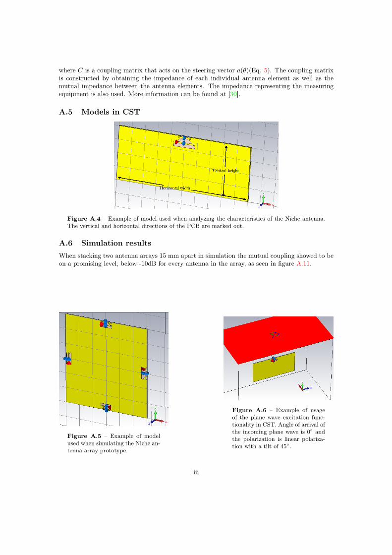
where C is a coupling matrix that acts on the steering vector a(θ)(Eq. 5). The coupling matrixis constructed by obtaining the impedance of each individual antenna element as well as themutual impedance between the antenna elements. The impedance representing the measuringequipment is also used. More information can be found at [30].

A.5 Models in CST

Figure A.4 – Example of model used when analyzing the characteristics of the Niche antenna.The vertical and horizontal directions of the PCB are marked out.

A.6 Simulation resultsWhen stacking two antenna arrays 15 mm apart in simulation the mutual coupling showed to beon a promising level, below -10dB for every antenna in the array, as seen in figure A.11.

Figure A.5 – Example of modelused when simulating the Niche an-tenna array prototype.

Figure A.6 – Example of usageof the plane wave excitation func-tionality in CST. Angle of arrival ofthe incoming plane wave is 0 andthe polarization is linear polariza-tion with a tilt of 45.

iii

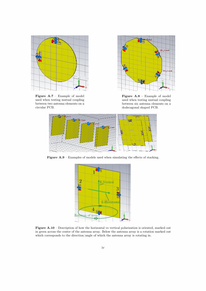
Figure A.7 – Example of modelused when testing mutual couplingbetween two antenna elements on acircular PCB.

Figure A.8 – Example of modelused when testing mutual couplingbetween six antenna elements on adodecagonal shaped PCB.

Figure A.9 – Examples of models used when simulating the effects of stacking.

Figure A.10 – Description of how the horizontal vs vertical polarization is oriented, marked outin green across the center of the antenna array. Below the antenna array is a rotation marked outwhich corresponds to the direction/angle of which the antenna array is rotating in.

iv

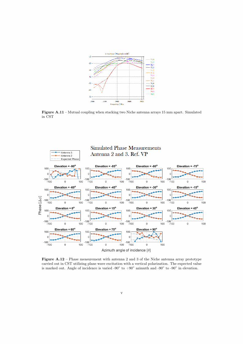
Figure A.11 – Mutual coupling when stacking two Niche antenna arrays 15 mm apart. Simulatedin CST

Figure A.12 – Phase measurement with antenna 2 and 3 of the Niche antenna array prototypecarried out in CST utilizing plane wave excitation with a vertical polarization. The expected valueis marked out. Angle of incidence is varied -90 to +90 azimuth and -90 to -90 in elevation.

v

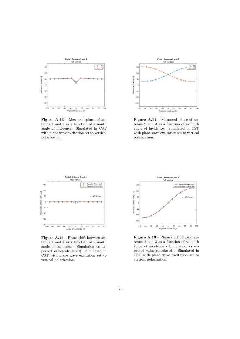
Figure A.13 – Measured phase of an-tenna 1 and 4 as a function of azimuthangle of incidence. Simulated in CSTwith plane wave excitation set to verticalpolarization.

Figure A.14 – Measured phase of an-tenna 2 and 3 as a function of azimuthangle of incidence. Simulated in CSTwith plane wave excitation set to verticalpolarization.

Figure A.15 – Phase shift between an-tenna 1 and 4 as a function of azimuthangle of incidence - Simulation vs ex-pected value(calculated). Simulated inCST with plane wave excitation set tovertical polarization.

Figure A.16 – Phase shift between an-tenna 2 and 3 as a function of azimuthangle of incidence - Simulation vs ex-pected value(calculated). Simulated inCST with plane wave excitation set tovertical polarization.

vi

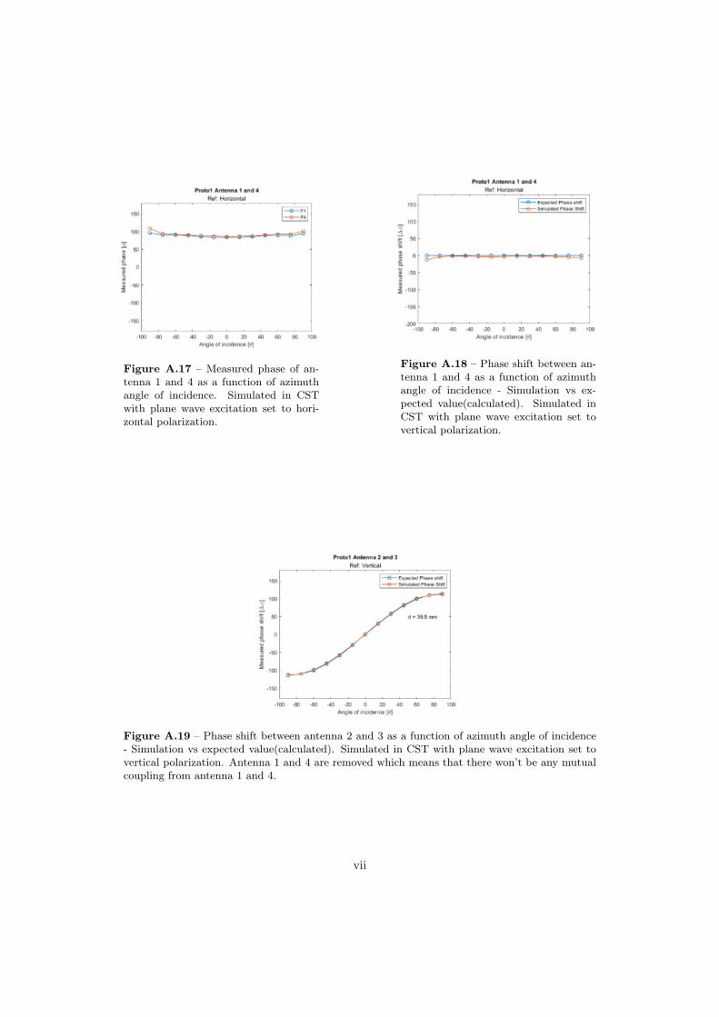
Figure A.17 – Measured phase of an-tenna 1 and 4 as a function of azimuthangle of incidence. Simulated in CSTwith plane wave excitation set to hori-zontal polarization.

Figure A.18 – Phase shift between an-tenna 1 and 4 as a function of azimuthangle of incidence - Simulation vs ex-pected value(calculated). Simulated inCST with plane wave excitation set tovertical polarization.

Figure A.19 – Phase shift between antenna 2 and 3 as a function of azimuth angle of incidence- Simulation vs expected value(calculated). Simulated in CST with plane wave excitation set tovertical polarization. Antenna 1 and 4 are removed which means that there won’t be any mutualcoupling from antenna 1 and 4.

vii